Embed Size (px)
Citation preview

Power Electronics Design:
A Practitioner’s Guide

Power Electronics Design:
A Practitioner’s Guide
Keith H. Sueker
AMSTERDAM • BOSTON • HEIDELBERG • LONDONNEW YORK • OXFORD • PARIS • SAN DIEGO
SAN FRANCISCO • SINGAPORE • SYDNEY • TOKYO
Newnes is an imprint of Elsevier
Newnes is an imprint of Elsevier30 Corporate Drive, Suite 400, Burlington, MA 01803, USALinacre House, Jordan Hill, Oxford OX2 8DP, UK
Copyright © 2005, SciTech Publishing Inc. 911 Paverstone Dr., Ste. BRaleigh, NC 27615www.scitechpub.com
All rights reserved.
No part of this publication may be reproduced, stored in a retrieval system, ortransmitted in any form or by any means, electronic, mechanical, photocopying,recording, or otherwise, without the prior written permission of the publisher.
Permissions may be sought directly from Elsevier’s Science & Technology RightsDepartment in Oxford, UK: phone: (+44) 1865 843830, fax: (+44) 1865 853333,e-mail: [email protected]. You may also complete your request onlinevia the Elsevier homepage (http://www.elsevier.com), by selecting “CustomerSupport” and then “Obtaining Permissions.”
Tables 14.4 and 14.5 reprinted with permission from IEEE Std. 519-1992–Recommended Practices and Requirements for Harmonic Control in Electrical Power Systems, Copyright 1996
©
, by IEEE. The IEEE disclaims any responsibility or liability resulting from the placement and use in the described manner.
Recognizing the importance of preserving what has been written,Elsevier prints its books on acid-free paper whenever possible.
Library of Congress Cataloging-in-Publication Data
Sueker, Keith H. Power electronics design : a practitioner's guide / by Keith H. Sueker.—1st ed. p. cm. Includes bibliographical references and index. ISBN 0-7506-7927-1 (hardcover : alk. paper) 1. Power electronics—Design
and construction. I. Title. TK7881.15.S84 2005 621.31'7--dc22 2005013673
British Library Cataloguing-in-Publication Data
A catalogue record for this book is available from the British Library.
ISBN: 0-7506-7946-8
For information on all Newnes publicationsvisit our website at www.books.elsevier.com
05 06 07 08 09 10 10 9 8 7 6 5 4 3 2 1
Printed in the United States of America
v
Contents
List of Figures. . . . . . . . . . . . . . . . . . . . . . . . . . . . . . . . . . . . . . . . . . xi
List of Tables . . . . . . . . . . . . . . . . . . . . . . . . . . . . . . . . . . . . . . . . xvii
Preface. . . . . . . . . . . . . . . . . . . . . . . . . . . . . . . . . . . . . . . . . . . . . . . xix
Chapter 1 Electric Power . . . . . . . . . . . . . . . . . . . . . . . . . . . . . . . .1
1.1 AC versus DC . . . . . . . . . . . . . . . . . . . . . . . . . . . . . . . . . . . . . . . .11.2 Pivotal Inventions . . . . . . . . . . . . . . . . . . . . . . . . . . . . . . . . . . . . .31.3 Generation. . . . . . . . . . . . . . . . . . . . . . . . . . . . . . . . . . . . . . . . . . .41.4 Electric Traction . . . . . . . . . . . . . . . . . . . . . . . . . . . . . . . . . . . . . .51.5 Electric Utilities . . . . . . . . . . . . . . . . . . . . . . . . . . . . . . . . . . . . . .61.6 In-Plant Distribution . . . . . . . . . . . . . . . . . . . . . . . . . . . . . . . . . .111.7 Emergency Power . . . . . . . . . . . . . . . . . . . . . . . . . . . . . . . . . . . .12
Chapter 2 Power Apparatus . . . . . . . . . . . . . . . . . . . . . . . . . . . .15
2.1 Switchgear. . . . . . . . . . . . . . . . . . . . . . . . . . . . . . . . . . . . . . . . . .152.2 Surge Suppression. . . . . . . . . . . . . . . . . . . . . . . . . . . . . . . . . . . .192.3 Conductors . . . . . . . . . . . . . . . . . . . . . . . . . . . . . . . . . . . . . . . . .212.4 Capacitors . . . . . . . . . . . . . . . . . . . . . . . . . . . . . . . . . . . . . . . . . .252.5 Resistors . . . . . . . . . . . . . . . . . . . . . . . . . . . . . . . . . . . . . . . . . . .282.6 Fuses . . . . . . . . . . . . . . . . . . . . . . . . . . . . . . . . . . . . . . . . . . . . . .312.7 Supply Voltages . . . . . . . . . . . . . . . . . . . . . . . . . . . . . . . . . . . . .32
vi Contents
2.8 Enclosures . . . . . . . . . . . . . . . . . . . . . . . . . . . . . . . . . . . . . . . . . .322.9 Hipot, Corona, and BIL. . . . . . . . . . . . . . . . . . . . . . . . . . . . . . . .332.10 Spacings . . . . . . . . . . . . . . . . . . . . . . . . . . . . . . . . . . . . . . . . . . .342.11 Metal Oxide Varistors . . . . . . . . . . . . . . . . . . . . . . . . . . . . . . . . .352.12 Protective Relays. . . . . . . . . . . . . . . . . . . . . . . . . . . . . . . . . . . . .37
Chapter 3 Analytical Tools. . . . . . . . . . . . . . . . . . . . . . . . . . . . . .39
3.1 Symmetrical Components . . . . . . . . . . . . . . . . . . . . . . . . . . . . . .393.2 Per Unit Constants. . . . . . . . . . . . . . . . . . . . . . . . . . . . . . . . . . . .413.3 Circuit Simulation . . . . . . . . . . . . . . . . . . . . . . . . . . . . . . . . . . . .433.4 Circuit Simulation Notes. . . . . . . . . . . . . . . . . . . . . . . . . . . . . . .453.5 Simulation Software . . . . . . . . . . . . . . . . . . . . . . . . . . . . . . . . . .47
Chapter 4 Feedback Control Systems . . . . . . . . . . . . . . . . . . . . .49
4.1 Basics . . . . . . . . . . . . . . . . . . . . . . . . . . . . . . . . . . . . . . . . . . . . .494.2 Amplitude Responses . . . . . . . . . . . . . . . . . . . . . . . . . . . . . . . . .504.3 Phase Responses . . . . . . . . . . . . . . . . . . . . . . . . . . . . . . . . . . . . .534.4 PID Regulators . . . . . . . . . . . . . . . . . . . . . . . . . . . . . . . . . . . . . .544.5 Nested Control Loops . . . . . . . . . . . . . . . . . . . . . . . . . . . . . . . . .56
Chapter 5 Transients . . . . . . . . . . . . . . . . . . . . . . . . . . . . . . . . . .57
5.1 Line Disturbances . . . . . . . . . . . . . . . . . . . . . . . . . . . . . . . . . . . .575.2 Circuit Transients . . . . . . . . . . . . . . . . . . . . . . . . . . . . . . . . . . . .585.3 Electromagnetic Interference . . . . . . . . . . . . . . . . . . . . . . . . . . .61
Chapter 6 Traveling Waves . . . . . . . . . . . . . . . . . . . . . . . . . . . . .65
6.1 Basics . . . . . . . . . . . . . . . . . . . . . . . . . . . . . . . . . . . . . . . . . . . . .656.2 Transient Effects . . . . . . . . . . . . . . . . . . . . . . . . . . . . . . . . . . . . .686.3 Mitigating Measures . . . . . . . . . . . . . . . . . . . . . . . . . . . . . . . . . .71
Chapter 7 Transformers and Reactors . . . . . . . . . . . . . . . . . . . .73
7.1 Transformer Basics . . . . . . . . . . . . . . . . . . . . . . . . . . . . . . . . . . .747.2 Construction . . . . . . . . . . . . . . . . . . . . . . . . . . . . . . . . . . . . . . . .787.3 Insulation Systems. . . . . . . . . . . . . . . . . . . . . . . . . . . . . . . . . . . .827.4 Basic Insulation Level . . . . . . . . . . . . . . . . . . . . . . . . . . . . . . . . .847.5 Eddy Current Effects . . . . . . . . . . . . . . . . . . . . . . . . . . . . . . . . . .857.6 Interphase Transformers . . . . . . . . . . . . . . . . . . . . . . . . . . . . . . .897.7 Transformer Connections . . . . . . . . . . . . . . . . . . . . . . . . . . . . . .907.8 Reactors. . . . . . . . . . . . . . . . . . . . . . . . . . . . . . . . . . . . . . . . . . . .93
Contents vii
7.9 Units . . . . . . . . . . . . . . . . . . . . . . . . . . . . . . . . . . . . . . . . . . . . . .977.10 Cooling . . . . . . . . . . . . . . . . . . . . . . . . . . . . . . . . . . . . . . . . . . . .977.11 Instrument Transformers. . . . . . . . . . . . . . . . . . . . . . . . . . . . . . .98
Chapter 8 Rotating Machines . . . . . . . . . . . . . . . . . . . . . . . . . .101
8.1 Direct Current Machines. . . . . . . . . . . . . . . . . . . . . . . . . . . . . .1018.2 Synchronous Machines . . . . . . . . . . . . . . . . . . . . . . . . . . . . . . .1038.3 Induction (Asynchronous) Machines . . . . . . . . . . . . . . . . . . . .1078.4 NEMA Designs. . . . . . . . . . . . . . . . . . . . . . . . . . . . . . . . . . . . .1108.5 Frame Types . . . . . . . . . . . . . . . . . . . . . . . . . . . . . . . . . . . . . . .1118.6 Linear Motors . . . . . . . . . . . . . . . . . . . . . . . . . . . . . . . . . . . . . .112
Chapter 9 Rectifiers and Converters. . . . . . . . . . . . . . . . . . . . .115
9.1 Early Rectifiers . . . . . . . . . . . . . . . . . . . . . . . . . . . . . . . . . . . . .1159.2 Mercury Vapor Rectifiers . . . . . . . . . . . . . . . . . . . . . . . . . . . . .1169.3 Silicon Diodes—The Semiconductor Age . . . . . . . . . . . . . . . .1179.4 Rectifier Circuits—Single-Phase . . . . . . . . . . . . . . . . . . . . . . .1189.5 Rectifier Circuits—Multiphase. . . . . . . . . . . . . . . . . . . . . . . . .1209.6 Commutation. . . . . . . . . . . . . . . . . . . . . . . . . . . . . . . . . . . . . . .123
Chapter 10 Phase Control . . . . . . . . . . . . . . . . . . . . . . . . . . . . .125
10.1 The SCR . . . . . . . . . . . . . . . . . . . . . . . . . . . . . . . . . . . . . . . . . .12610.2 Forward Drop . . . . . . . . . . . . . . . . . . . . . . . . . . . . . . . . . . . . . .13110.3 SCR Circuits—AC Switches . . . . . . . . . . . . . . . . . . . . . . . . . .13110.4 SCR Motor Starters. . . . . . . . . . . . . . . . . . . . . . . . . . . . . . . . . .13510.5 SCR Converters . . . . . . . . . . . . . . . . . . . . . . . . . . . . . . . . . . . .13710.6 Inversion . . . . . . . . . . . . . . . . . . . . . . . . . . . . . . . . . . . . . . . . . .13910.7 Gate Drive Circuits . . . . . . . . . . . . . . . . . . . . . . . . . . . . . . . . . .14210.8 Power to the Gates . . . . . . . . . . . . . . . . . . . . . . . . . . . . . . . . . .14510.9 SCR Autotapchangers. . . . . . . . . . . . . . . . . . . . . . . . . . . . . . . .14510.10 SCR DC Motor Drives . . . . . . . . . . . . . . . . . . . . . . . . . . . . . . .14810.11 SCR AC Motor Drives . . . . . . . . . . . . . . . . . . . . . . . . . . . . . . .14810.12 Cycloconverters . . . . . . . . . . . . . . . . . . . . . . . . . . . . . . . . . . . .150
Chapter 11 Series and Parallel Operation . . . . . . . . . . . . . . . .153
11.1 Voltage Sharing . . . . . . . . . . . . . . . . . . . . . . . . . . . . . . . . . . . .15311.2 Current Sharing. . . . . . . . . . . . . . . . . . . . . . . . . . . . . . . . . . . . .15811.3 Forced Sharing . . . . . . . . . . . . . . . . . . . . . . . . . . . . . . . . . . . . .160
viii Contents
Chapter 12 Pulsed Converters . . . . . . . . . . . . . . . . . . . . . . . . . .163
12.1 Protective Devices. . . . . . . . . . . . . . . . . . . . . . . . . . . . . . . . . . .16312.2 Transformers . . . . . . . . . . . . . . . . . . . . . . . . . . . . . . . . . . . . . . .16412.3 SCRs . . . . . . . . . . . . . . . . . . . . . . . . . . . . . . . . . . . . . . . . . . . . .166
Chapter 13 Switchmode Systems . . . . . . . . . . . . . . . . . . . . . . . .169
13.1 Pulse Width Modulation . . . . . . . . . . . . . . . . . . . . . . . . . . . . . .16913.2 Choppers . . . . . . . . . . . . . . . . . . . . . . . . . . . . . . . . . . . . . . . . . .17313.3 Boost Converters . . . . . . . . . . . . . . . . . . . . . . . . . . . . . . . . . . . .17413.4 The “H” Bridge . . . . . . . . . . . . . . . . . . . . . . . . . . . . . . . . . . . . .17513.5 High-Frequency Operation . . . . . . . . . . . . . . . . . . . . . . . . . . . .17813.6 Harmonic Injection . . . . . . . . . . . . . . . . . . . . . . . . . . . . . . . . . .17913.7 Series Bridges . . . . . . . . . . . . . . . . . . . . . . . . . . . . . . . . . . . . . .180
Chapter 14 Power Factor and Harmonics . . . . . . . . . . . . . . . .181
14.1 Power Factor . . . . . . . . . . . . . . . . . . . . . . . . . . . . . . . . . . . . . . .18114.2 Harmonics . . . . . . . . . . . . . . . . . . . . . . . . . . . . . . . . . . . . . . . . .18414.3 Fourier Transforms . . . . . . . . . . . . . . . . . . . . . . . . . . . . . . . . . .18914.4 Interactions with the Utility. . . . . . . . . . . . . . . . . . . . . . . . . . . .19414.5 Telephone Influence Factor. . . . . . . . . . . . . . . . . . . . . . . . . . . .19914.6 Distortion Limits . . . . . . . . . . . . . . . . . . . . . . . . . . . . . . . . . . . .20114.7 Zero-Switching . . . . . . . . . . . . . . . . . . . . . . . . . . . . . . . . . . . . .202
Chapter 15 Thermal Considerations . . . . . . . . . . . . . . . . . . . . .203
15.1 Heat and Heat Transfer . . . . . . . . . . . . . . . . . . . . . . . . . . . . . . .20315.2 Air Cooling . . . . . . . . . . . . . . . . . . . . . . . . . . . . . . . . . . . . . . . .20515.3 Water Cooling . . . . . . . . . . . . . . . . . . . . . . . . . . . . . . . . . . . . . .20615.4 Device Cooling . . . . . . . . . . . . . . . . . . . . . . . . . . . . . . . . . . . . .20815.5 Semiconductor Mounting . . . . . . . . . . . . . . . . . . . . . . . . . . . . .213
Chapter 16 Power Electronics Applications . . . . . . . . . . . . . . .215
16.1 Motor Drives and SCR Starters. . . . . . . . . . . . . . . . . . . . . . . . .21516.2 Glass Industry . . . . . . . . . . . . . . . . . . . . . . . . . . . . . . . . . . . . . .21716.3 Foundry Operations. . . . . . . . . . . . . . . . . . . . . . . . . . . . . . . . . .21816.4 Plasma Arcs and Arc Furnaces . . . . . . . . . . . . . . . . . . . . . . . . .21916.5 Electrochemical Supplies . . . . . . . . . . . . . . . . . . . . . . . . . . . . .21916.6 Cycloconverters. . . . . . . . . . . . . . . . . . . . . . . . . . . . . . . . . . . . .22016.7 Extremely Low-Frequency Communications . . . . . . . . . . . . . .221
Contents ix
16.8 Superconducting Magnet Energy Storage . . . . . . . . . . . . . . . .22216.9 600-kW Opamp. . . . . . . . . . . . . . . . . . . . . . . . . . . . . . . . . . . . .22316.10 Ozone Generators . . . . . . . . . . . . . . . . . . . . . . . . . . . . . . . . . . .22316.11 Semiconductor Silicon . . . . . . . . . . . . . . . . . . . . . . . . . . . . . . .22416.12 VAR Compensators . . . . . . . . . . . . . . . . . . . . . . . . . . . . . . . . .22416.13 Induction Furnace Switch . . . . . . . . . . . . . . . . . . . . . . . . . . . . .22516.14 Tokamaks . . . . . . . . . . . . . . . . . . . . . . . . . . . . . . . . . . . . . . . . .22616.15 Multi-tap Switching . . . . . . . . . . . . . . . . . . . . . . . . . . . . . . . . .227
Appendix A Converter Equations . . . . . . . . . . . . . . . . . . . . . . .229
Appendix B Lifting Forces . . . . . . . . . . . . . . . . . . . . . . . . . . . . .231
Appendix C Commutation Notches and THDv . . . . . . . . . . . .233
Appendix D Capacitor Ratings . . . . . . . . . . . . . . . . . . . . . . . . .235
Appendix E Rogowski Coils . . . . . . . . . . . . . . . . . . . . . . . . . . . .237
Appendix F Foreign Technical Words . . . . . . . . . . . . . . . . . . .239
Appendix G Aqueous Glycol Solutions . . . . . . . . . . . . . . . . . . .241
Appendix H Harmonic Cancellation with Phase Shifting . . . .243
Appendix I Neutral Currents with Nonsinusoidal Loads . . . .245
Index . . . . . . . . . . . . . . . . . . . . . . . . . . . . . . . . . . . . . . . . . . . . . . . . 247


xi
List of Figures
Figure 1.1 Generation systems. .................................................3Figure 1.2 Typical section of a utility. ......................................7Figure 2.1 Power electronics symbols.....................................16Figure 2.2 Typical wire labeling. ............................................22Figure 2.3 Stress cone termination for shielded cable.............24Figure 2.4 Capacitor construction. ..........................................27Figure 2.5 Power resistor types. ..............................................30Figure 2.6 Simple corona tester...............................................34Figure 2.7 480-V, 60-mm MOV characteristic. ......................36Figure 3.1 Symmetrical components.......................................41Figure 3.2 Arc heater circuit....................................................44Figure 3.3 Circuit voltage and current waveforms..................44Figure 4.1 Basic feedback system. ..........................................49Figure 4.2 R/C frequency response. ........................................51Figure 4.3 Frequency responses of various networks. ............51Figure 4.4 Composite response. ..............................................52Figure 4.5 Frequency responses, F(s), and corresponding
time responses, f(t).................................................52Figure 4.6 Phase responses of an R/C low-pass filter. ............54Figure 4.7 Phase lag of a 1.4-ms transport lag. .......................55Figure 4.8 PID regulator..........................................................55

xii List of Figures
Figure 4.9 Nested control loops. .............................................56Figure 5.1 Signal wire routing.................................................59Figure 5.2 R/C notch reduction filter. .....................................60Figure 5.3 Multiplier input filtering. .......................................61Figure 5.4 T-section filter........................................................62Figure 5.5 Shunt wiring...........................................................62Figure 5.6 Preferred shunt construction. .................................63Figure 6.1 Transmission line difference equations. ................67Figure 6.2 Transmission line parameters. ...............................67Figure 6.3 Transmission line reflections—open load. ............69Figure 6.4 Front-of-wave shaping. ..........................................70Figure 6.5 Overshoot as a function of rise time. .....................71Figure 7.1 Coupled coils. ........................................................74Figure 7.2 Ideal transformer. ...................................................75Figure 7.3 Typical transformer representation. .......................76Figure 7.4 Transformer regulation phasor diagram.................77Figure 7.5 Three-winding transformer. ...................................78Figure 7.6 Transformer cross sections. ...................................79Figure 7.7 Split bobbin transformer. .......................................83Figure 7.8 Surge voltage distribution in a transformer
winding. .................................................................85Figure 7.9 Transposition to reduce eddy currents. ..................86Figure 7.10 Eddy currents in lamination iron............................86Figure 7.11 Eddy current losses in windings. ...........................88Figure 7.12 Eddy current heating in shield materials................89Figure 7.13 Two- and three-leg interphase transformer
cores. ......................................................................90Figure 7.14 Autotransformer connections.................................91Figure 7.15 Transformer primary taps. .....................................91Figure 7.16 Paralleled transformers. .........................................92Figure 7.17 Phase-shifted secondaries, 24-pulse.......................93Figure 7.18 Basic equations for an inductive circuit.................94Figure 7.19 Inductance of a single-layer solenoid. ...................94Figure 7.20 Inductance of a short, fat, multilayer coil. .............95Figure 7.21 Inductance of a thin, flat, spiral coil. .....................95Figure 7.22 Inductance of a single-layer toroidal coil...............95
List of Figures xiii
Figure 7.23 Elementary iron-core conductor. ...........................96Figure 7.24 Three-phase inductance measurement. ..................96Figure 7.25 Skirting to improve transformer cooling................98Figure 8.1 DC motor characteristics......................................102Figure 8.2 DC motor control. ................................................103Figure 8.3 Generator phasor diagram....................................104Figure 8.4 Generator and motor torque angles......................106Figure 8.5 Induction motor equivalent circuit.......................108Figure 8.6 Induction motor torque and current. ....................108Figure 8.7 Supersynchronous operation................................109Figure 8.8 NEMA design torque curves................................111Figure 8.9 Induction motor frame types................................111Figure 8.10 Elementary rail gun..............................................113Figure 9.1 Half-wave rectifier characteristics. ......................118Figure 9.2 Full-wave, center-tapped rectifier circuit and
waveforms............................................................120Figure 9.3 Single-phase bridge (double-way) rectifier and
waveforms............................................................121Figure 9.4 Three-phase double-wye interphase and bridge
rectifier circuit......................................................121Figure 9.5 Commutation in a three-phase bridge rectifier. ...123Figure 10.1 SCR characteristics. .............................................126Figure 10.2 Typical SCR gate drive........................................127Figure 10.3 SCR recovery characteristics. ..............................128Figure 10.4 Equivalent SCR recovery circuit and
difference equations. ............................................129Figure 10.5 Single-phase SCR AC switch. .............................132Figure 10.6 SCR single-phase AC switch waveforms. ...........132Figure 10.7 Three-phase SCR AC switches............................133Figure 10.8 Three-phase AC switch, 60° phaseback,
0.8 pf lagging load. ..............................................134Figure 10.9 Three-phase AC switch, 120° phaseback,
0.8 pf lagging load. ..............................................134Figure 10.10 Starting characteristic of induction motor with
SCR starter. ..........................................................136Figure 10.11 Speed profile with SCR starter. ...........................137
xiv List of Figures
Figure 10.12 SCR three-phase bridge converter. ......................138Figure 10.13 Converter L-N voltages and line currents
(inductive load). ...................................................139Figure 10.14 Converter bus voltages.........................................139Figure 10.15 Converter line-to-line voltage. .............................140Figure 10.16 Converter DC output voltage. ..............................140Figure 10.17 Converter DC inversion at 150° phaseback. ........141Figure 10.18 Cosine intercept SCR gate drive. .........................143Figure 10.19 SCR autotapchanger.............................................146Figure 10.20 Displacement power factors.................................147Figure 10.21 Reversing, regenerative SCR DC motor drive.....148Figure 10.22 SCR current source inverter AC drive. ................149Figure 10.23 SCR load-commutated inverter AC drive............150Figure 11.1 High-level gate drive............................................154Figure 11.2 Series SCR gate drive arrangements....................155Figure 11.3 Anode-cathode derived gating. ............................156Figure 11.4 Series SCR recovery characteristics. ...................156Figure 11.5 Sharing network for series SCRs. ........................157Figure 11.6 Bus layouts...........................................................158Figure 11.7 Self and mutual inductances. ...............................159Figure 11.8 Sharing reactors. ..................................................160Figure 13.1 Basic pulse width modulation..............................170Figure 13.2 IGBT schematic and characteristics.....................172Figure 13.3 Chopper circuit and waveforms. ..........................173Figure 13.4 Ripple in paralleled choppers...............................174Figure 13.5 Chopper at 50% duty cycle. .................................175Figure 13.6 IGBT boost converter. .........................................175Figure 13.7 “H” bridge............................................................176Figure 13.8 PWM sine wave switching...................................176Figure 13.9 IGBT motor drive. ...............................................177Figure 13.10 Chopper-controlled 30-kHz inverter....................178Figure 13.11 Harmonic injection...............................................179Figure 13.12 2400-V, 18-pulse series bridges...........................180Figure 14.1 Demand multiplier. ..............................................182Figure 14.2 Power factor correction........................................183Figure 14.3 Fundamental with third harmonic........................186
List of Figures xv
Figure 14.4 SCR DC motor drive waveforms.........................187Figure 14.5 SCR DC motor drive characteristics....................188Figure 14.6 Transforms in the complex plane.........................189Figure 14.7 Transforms of pulses............................................189Figure 14.8 Fourier transforms................................................190Figure 14.9 Fourier transform for a symmetrical
waveform. ............................................................190Figure 14.10 Duty cycle rms value. ..........................................191Figure 14.11 Six-pulse and 12-pulse harmonic spectra. ...........194Figure 14.12 Harmonic resonance.............................................195Figure 14.13 Harmonic trap results. ..........................................197Figure 14.14 High-pass filters. ..................................................198Figure 14.15 Current and voltage distortion. ............................199Figure 15.1 Fan delivery curves. .............................................206Figure 15.2 Basic water cooling system..................................207Figure 15.3 Transient thermal impedance curves. ..................211Figure 15.4 Thermal network elements...................................212Figure 15.5 Composite thermal network.................................213Figure 15.6 SCR transient junction temperature rise. .............213Figure 16.1 Rod furnace autotapchanger supply.....................218Figure 16.2 Typical electrochemical supply. ..........................220Figure 16.3 Three-phase cycloconverter. ................................221Figure 16.4 ELF transmitter. ...................................................222Figure 16.5 600-kW Opamp....................................................223Figure 16.6 VAR compensator and control range...................225Figure 16.7 Solid-state contactor.............................................226Figure 16.8 Autotapchanger performance...............................227Figure 16.9 Wide-range, zero-switched tap changer...............228Figure A.1 Single line diagram. .............................................229Figure B.1 Lifting forces and moments. ................................232Figure C.1 Voltage distortion waveform. ..............................233Figure E.1 Rogowski coil construction..................................237Figure G.1 Properties of ethylene and propylene glycol
aqueous mixtures. ................................................242

xvii
List of Tables
Table 2.1 Switchgear Electrical Clearance Standards ...............35Table 7.1 Transformer Characteristics.......................................81Table 7.2 Insulation Classes.......................................................82Table 7.3 Air-Core/Iron-Core Inductor Comparisons................93Table 7.4 Self and Mutual Inductances......................................95Table 7.5 Magnetic Units...........................................................97Table 10.1 Converter Equations.................................................142Table 14.1 Energy and Demand.................................................182Table 14.2 Equal Tempered Chromatic Scale ...........................185Table 14.3 Square Wave RMS Synthesis ..................................192Table 14.4 Single-Frequency TIF Values, IEEE 519 ................200Table 14.5 Current Distortion Limits for General
Distribution Systems, IEEE 519 (120 through 69,000 V) .................................................................201
Table 14.6 Zero-Switching Spectra ...........................................202Table 15.1 Thermal Constants ...................................................204Table 15.2 Radiation Emissivities of Common Materials .........205Table F.1 Foreign Technical Words.........................................239


xix
Preface
I have presented numerous courses in the form of noontime tutorialsduring my career with Robicon Corporation. These covered suchessential subjects as transformers, transmission lines, heat transfer,transients, and semiconductors, to name but a few. The attendees weredesign engineers, sales engineers, technicians, and drafters. The tuto-rials were designed to present an overview of the power electronicsfield as well as design information for the engineers. They were verywell received and appreciated. The material was useful to design engi-neers, but the technicians, drafters, and sales engineers appreciatedthe fact that I did not talk over their heads. I have also given tutorialsto national meetings of the IEEE Industrial Applications Society aswell as local presentations. This book represents a consolidation andorganization of this material.
In this book, I have defined power electronics as the application ofhigh-power semiconductor technology to large motor drives, powersupplies, power conversion equipment, electric utility auxiliaries, anda host of other applications. It provides an overview of material nolonger taught in most college electrical engineering curricula, and itcontains a wealth of practical design information. It is also intendedas a reference book covering design considerations that are not obvi-
xx Preface
ous but are better not learned the hard way. It presents an overview ofthe ancillary apparatus associated with power electronics as well asexamples of potential pitfalls in the design process. The bookapproaches these matters in a simple, directed fashion with a mini-mum reliance on calculus. I have tried to put the overall design pro-cess into perspective as regards the primary electronic componentsand the many associated components that are required for a system.
My intended audience is design engineers, design drafters, andtechnicians now working in the power electronics industry. Studentsstudying in two- and four-year electrical engineering and engineeringtechnology programs, advanced students seeking a ready reference,and engineers working in other industries but with a need to knowsome essential aspects of power electronics will all find the book bothunderstandable and useful. Readers of this book will most appreciateits down-to-earth approach, freedom from jargon and esoteric or non-essential information, the many simple illustrations used to clarifydiscussion points, and the vivid examples of costly design goofs.
When I was in graduate school, I was given a copy of
The Westing-house Electrical Transmission and Distribution Reference Manual.
This book covered both theory and practice of the many aspects of thegeneration, transmission, and distribution of electric power. For meand thousands of engineers, it has been an invaluable reference bookfor all the years of my work in design. I hope to serve a similar func-tion with this book on power electronics.
Acknowledgments
I have attempted to write about the things I worked with during my 50years in industry. Part were spent with Westinghouse in magneticamplifiers and semiconductors and the last 30 with Robicon Corpora-tion, now ASIRobicon. I had the privilege of working with some verytalented engineers, and this book profits from their experiences aswell as my own. As Engineering Manager of the Power Systems

Preface xxi
group at Robicon, I had the best job in the world. My charge was sim-ply to make whatever would work and result in a profit for the com-pany. The understanding was that it would be at least looselyassociated with power semiconductors, although I drifted into a lineof medium-voltage, passive harmonic filters. Yes, we made money onthem. The other aspect of my job was to mentor and work with somevery talented young engineers. Their enthusiasm and hard work actu-ally made me look good. My thanks to Junior, Ken, Pete, Bob, Frank,Geoff, Frank, Joe, Mark, Joe, Gene, and John. I also owe a debt ofgratitude for the professional associations with Bob, Harry, Dick, andPete. I gratefully acknowledge the personnel at SciTech Publishing,who helped develop the book, and J. K. Eckert & Co., who performedthe editing and layout.
Lastly, I apologize for any errors and omissions and hope the bookwill prove useful in spite of them.
Keith H. Sueker, PE
Consulting EngineerPittsburgh, PA

1
Chapter 1
Electric Power
Relative to the digital age, the electric utility industry may seem oldhat. But power electronics and the power industry have a growingsymbiotic relationship. Nearly all power electronics systems drawpower from the grid, and utility companies benefit from the applica-tion of power electronics to motor drives and to converters used forhigh-voltage DC transmission lines. The two fields are very much in astate of constant development of new systems and applications. Forthat reason, a short review of the history and the present state of theelectric utility industry is appropriate for consideration by the powerelectronics engineer.
1.1. AC versus DC
Take warning! Alternating currents are dangerous. They are fitonly for powering the electric chair. The only similarity betweenan a-c and a d-c lighting system is that they both start from thesame coal pile.
And thus did Thomas Edison try to discourage the growing use ofalternating-current electric power that was competing with his DC
2 1
◊
Electric Power
systems. Edison had pioneered the first true central generating stationat Pearl Street, in New York City, with DC. It had the ability to takegenerators on and off line and had a battery supply for periods of lowdemand. Distribution was at a few hundred volts, and the area servedwas confined because of the voltage drop in conductors of a reason-able size. The use of DC at relatively low voltages became a factorthat limited the geographic growth of the electric utilities, but DC waswell suited to local generation, and the use of electric power grew rap-idly. Direct current motors gradually replaced steam engines forpower in many industries. An individual machine could be driven byits own motor instead of having to rely on belting to a line shaft.
Low-speed reciprocating steam engines were the typical primemovers for the early generators, many being double-expansiondesigns in which a high-pressure cylinder exhausted steam to a low-pressure cylinder to improve efficiency. The double-expansion Corlissengines installed in 1903 for the IRT subway in New York developed7500 hp at 75 rpm. Generators were driven at a speed higher than theengine by means of pulleys with rope or leather belts. Storage batter-ies usually provided excitation for the generators and were themselvescharged from a small generator. DC machines could be paralleledsimply by matching the voltage of the incoming machine to the busvoltage and then switching it in. Load sharing was adjusted by fieldcontrol.
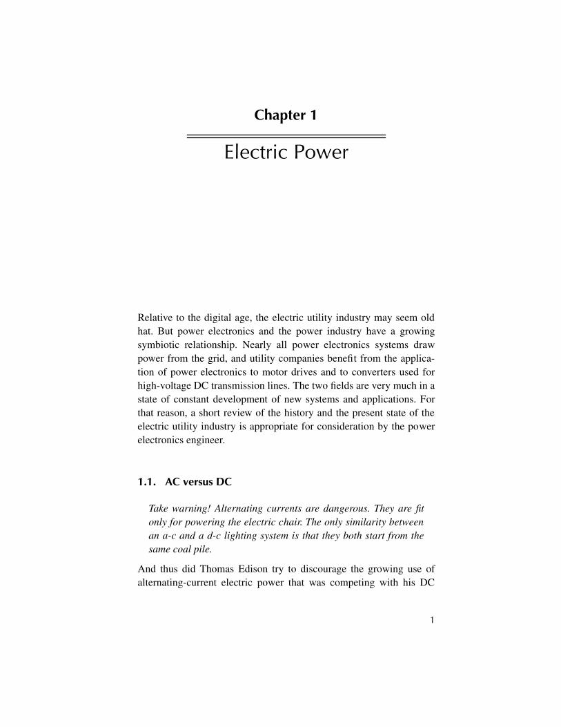
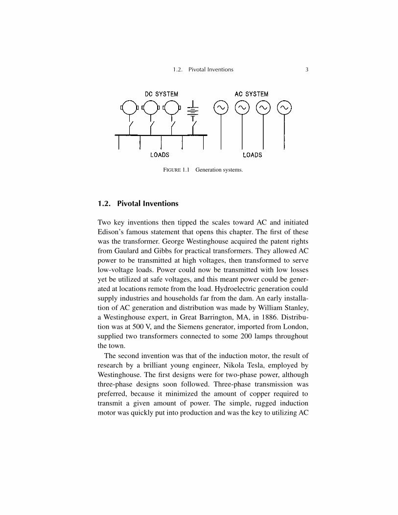
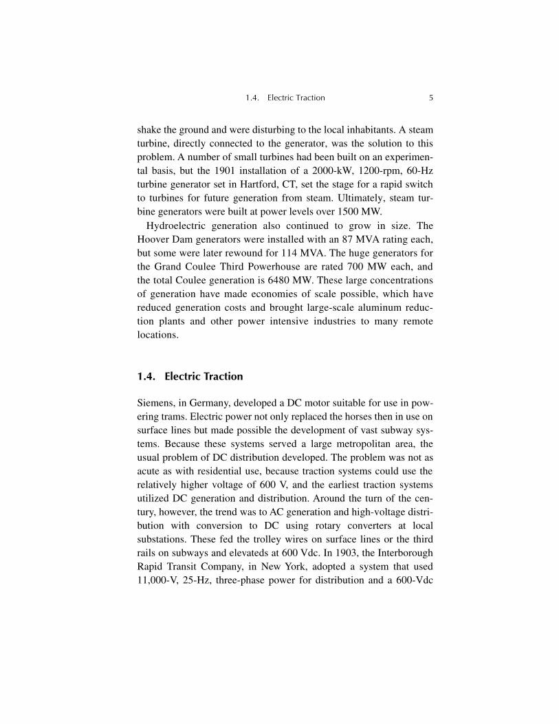
Alternating-current generators had been built for some years, butfurther use of AC power had been limited by the lack of a suitable ACmotor. Low-frequency AC could be used on commutator motors thatwere basically DC machines, but attempts to operate them on thehigher AC frequencies required to minimize lamp flicker were notsuccessful. Furthermore, early AC generators could be paralleled onlywith difficulty, so each generator had to be connected to an assignedload and be on line at all times. Battery backup or battery supply atlight load could not be used. Figure 1.1 shows the difference. Finally,generation and utilization voltages were similar to those with DC, soAC offered no advantage in this regard.
1.2. Pivotal Inventions 3
1.2. Pivotal Inventions
Two key inventions then tipped the scales toward AC and initiatedEdison’s famous statement that opens this chapter. The first of thesewas the transformer. George Westinghouse acquired the patent rightsfrom Gaulard and Gibbs for practical transformers. They allowed ACpower to be transmitted at high voltages, then transformed to servelow-voltage loads. Power could now be transmitted with low lossesyet be utilized at safe voltages, and this meant power could be gener-ated at locations remote from the load. Hydroelectric generation couldsupply industries and households far from the dam. An early installa-tion of AC generation and distribution was made by William Stanley,a Westinghouse expert, in Great Barrington, MA, in 1886. Distribu-tion was at 500 V, and the Siemens generator, imported from London,supplied two transformers connected to some 200 lamps throughoutthe town.
The second invention was that of the induction motor, the result ofresearch by a brilliant young engineer, Nikola Tesla, employed byWestinghouse. The first designs were for two-phase power, althoughthree-phase designs soon followed. Three-phase transmission waspreferred, because it minimized the amount of copper required totransmit a given amount of power. The simple, rugged inductionmotor was quickly put into production and was the key to utilizing AC
FIGURE 1.1 Generation systems.
4 1
◊
Electric Power
power by industry. The induction motor required no elaborate startingmeans, it was low in cost, and it offered important advantages in unfa-vorable environments. Together, the transformer and induction motorwere responsible for the rapid growth of AC power.
The superiority of AC power was proven when Westinghouselighted the Columbian Exposition at Chicago in 1893 with a two-phase system and literally turned night into day. Edison held the pat-ents on the glass sealed incandescent lamp, so Westinghouse devised astopper lamp design utilizing sealing wax. It was not a commerciallysuccessful design, but it did the job. The dazzling display was a sourceof awe for the visitors, many of whom had never seen an electric light.
A second major advance in AC generation and transmission was aninstallation at Niagara Falls. The power potential of the falls had beenrecognized for many years, and various schemes had been proposedfor using compressed air and mechanical methods to harness thepower. A final study resulted in the installation by Westinghouse in1895 of AC generators using a 25-Hz, two-phase system that incorpo-rated transformers and transmission lines to serve a number of facto-ries. The 25-Hz frequency was chosen despite the growing popularityof 60 Hz, because it was recognized that a number of the processindustries would require large amounts of DC power, and the rotaryconverters then used could not function on 60 Hz. Frequencies of 30,40, 50, and 133 Hz were also in use in the 1890s, and 50 Hz persisteduntil mid century on the Southern California Edison System. A num-ber of utilities also provided 25-Hz power late into the last century.
1.3. Generation
Slow-speed reciprocating steam engines kept growing in size to keepup with the demand for power until they topped out at around thecited 7500 hp. Some high-speed steam engines were used in England,but there was usually an order of magnitude difference between thepreferred speeds for the engine and for the generator. The huge steamengines in use around the beginning of the twentieth century would
1.4. Electric Traction 5
shake the ground and were disturbing to the local inhabitants. A steamturbine, directly connected to the generator, was the solution to thisproblem. A number of small turbines had been built on an experimen-tal basis, but the 1901 installation of a 2000-kW, 1200-rpm, 60-Hzturbine generator set in Hartford, CT, set the stage for a rapid switchto turbines for future generation from steam. Ultimately, steam tur-bine generators were built at power levels over 1500 MW.
Hydroelectric generation also continued to grow in size. TheHoover Dam generators were installed with an 87 MVA rating each,but some were later rewound for 114 MVA. The huge generators forthe Grand Coulee Third Powerhouse are rated 700 MW each, andthe total Coulee generation is 6480 MW. These large concentrationsof generation have made economies of scale possible, which havereduced generation costs and brought large-scale aluminum reduc-tion plants and other power intensive industries to many remotelocations.
1.4. Electric Traction
Siemens, in Germany, developed a DC motor suitable for use in pow-ering trams. Electric power not only replaced the horses then in use onsurface lines but made possible the development of vast subway sys-tems. Because these systems served a large metropolitan area, theusual problem of DC distribution developed. The problem was not asacute as with residential use, because traction systems could use therelatively higher voltage of 600 V, and the earliest traction systemsutilized DC generation and distribution. Around the turn of the cen-tury, however, the trend was to AC generation and high-voltage distri-bution with conversion to DC using rotary converters at localsubstations. These fed the trolley wires on surface lines or the thirdrails on subways and elevateds at 600 Vdc. In 1903, the InterboroughRapid Transit Company, in New York, adopted a system that used11,000-V, 25-Hz, three-phase power for distribution and a 600-Vdc
6 1
◊
Electric Power
third rail pickup for the cars of the new subway. Interestingly, thedirectors had decided in favor of reciprocating steam engines over tur-bines for generation, although they used several small turbine sets forlighting and excitation.
The use of electric power for transit also made possible interurbantrolley lines, and by the early years of the last century, vast networksof trolley systems were extended to serve many small communities atlower cost than the steam trains could achieve. Again, higher-voltageAC generation and distribution were coupled with rotary converters tosupply DC to the trolley wires. Interurban transit lines lasted until thedevelopment of good roads and reliable automobiles. Most were goneby mid century.
There were also a number of installations of electric motors to pro-vide power for main-line traction. The New York New Haven andHartford Railroad used 11,000-V, 25-Hz, three-phase power for trans-mission and single-phase power to supply the catenary. Transformerson the locomotives powered the traction motors in a parallel connec-tion at 250 Vac. The motors were then switched in series to operate ona 600 Vdc third-rail so the trains could continue into Manhattanunderground. The same distribution is in use today by Amtrak on theNortheast Corridor with the catenary supplied at 25 Hz by solid-statecycloconverters powered from the 60-Hz utility system. Several pio-neering electric railroads in the USA used 3000 Vdc on the catenary,and three-phase 25-Hz AC systems were also used. Nearly everyimaginable configuration of AC and DC power, including 16-2/3 Hz,was used for traction somewhere in the world. Except for commuterlines and special installations, most of the electric locomotives havebeen replaced by diesel electrics that offer lower operating costs andless overhead.
1.5. Electric Utilities
Utility operations are usually considered in the three classes of gen-eration, transmission, and distribution, although recent deregulation
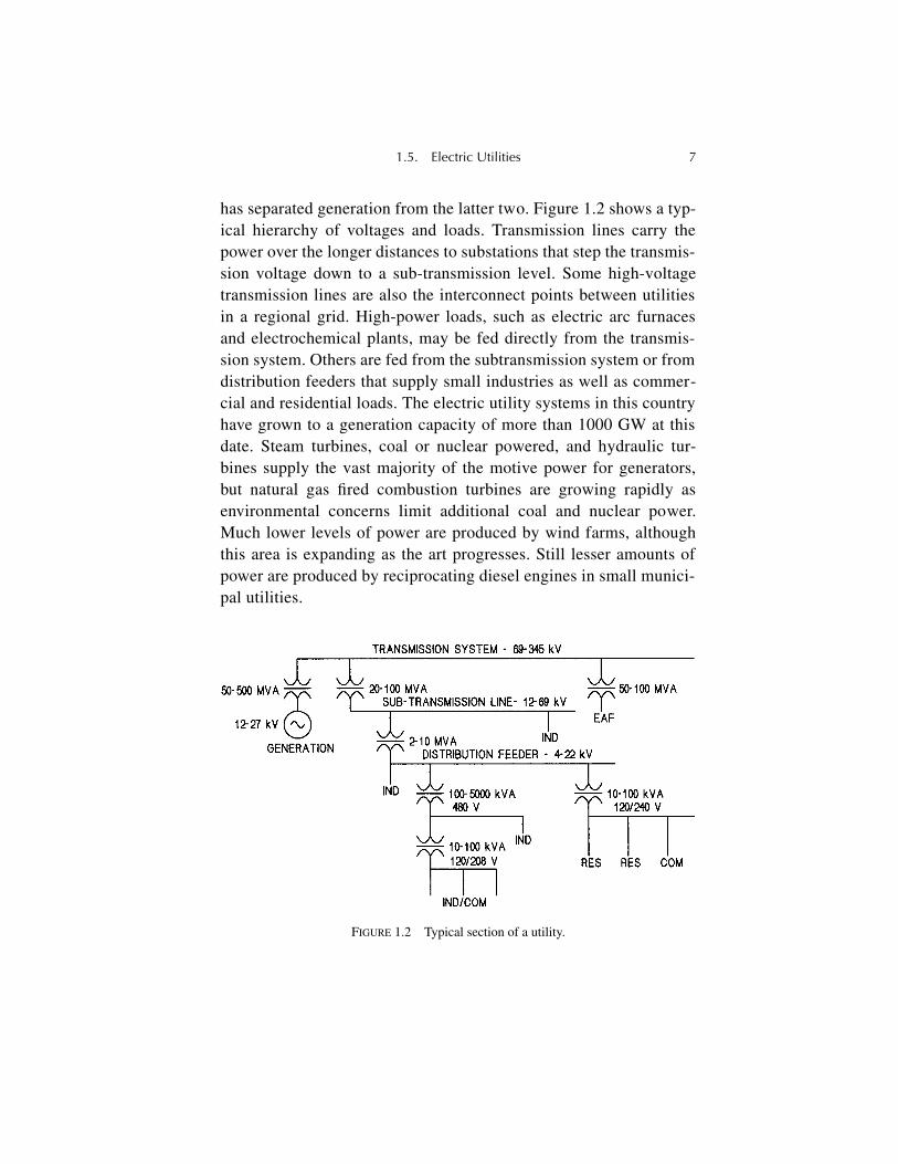
1.5. Electric Utilities 7
has separated generation from the latter two. Figure 1.2 shows a typ-ical hierarchy of voltages and loads. Transmission lines carry thepower over the longer distances to substations that step the transmis-sion voltage down to a sub-transmission level. Some high-voltagetransmission lines are also the interconnect points between utilitiesin a regional grid. High-power loads, such as electric arc furnacesand electrochemical plants, may be fed directly from the transmis-sion system. Others are fed from the subtransmission system or fromdistribution feeders that supply small industries as well as commer-cial and residential loads. The electric utility systems in this countryhave grown to a generation capacity of more than 1000 GW at thisdate. Steam turbines, coal or nuclear powered, and hydraulic tur-bines supply the vast majority of the motive power for generators,but natural gas fired combustion turbines are growing rapidly asenvironmental concerns limit additional coal and nuclear power.Much lower levels of power are produced by wind farms, althoughthis area is expanding as the art progresses. Still lesser amounts ofpower are produced by reciprocating diesel engines in small munici-pal utilities.
FIGURE 1.2 Typical section of a utility.
8 1
◊
Electric Power
The national transmission system is operated cooperatively byregional power pools of interconnected utilities, whereas generation,because of government regulation, is now in the hands of many inde-pendent operators. Transmission voltages increased over the years andtopped at around 230 kV for some time. The construction of theHoover Dam, however, made it possible to augment the Los Angelesenergy supply with hydroelectric power. When installed in the late1930s, this line was the longest and, at 287 kV, the highest voltageline in this country. A considerable amount of research went into theinsulation system and the conductor design to minimize coronalosses. Progressively higher transmission voltages have been intro-duced until switchgear standards have now been developed for800 kV service. Transmission lines at or above 500 kV are termedEHV for
extra high voltage
. A major EHV project in the U.S. is the905-mile Pacific Intertie from the Bonneville Power Administration inWashington to the Los Angeles area. Two 500-kV transmission linessupply some 2500 MW, bringing hydroelectric power from installa-tions on the Columbia River to the major load centers in SouthernCalifornia. Hydro-Québec operates a large system of 765-kV trans-mission lines to bring hydroelectric power from northern Québec toload centers in Canada and the U.S.
Although most transmission lines are referred to by their nominaltransmission voltage, they are designed for a given
basic insulationlevel (BIL)
in consideration of lightning strokes and switching tran-sients. Lightning strokes have been measured at voltages of 5 MV,currents of 220 kA, and a maximum dv/dt of 50 kA/µs, so they havethe potential for doing serious damage. Lightning arresters are dis-cussed in Chapter 2.
High-voltage DC (HVDC) transmission lines have come into ser-vice through the advent of power electronics. These have an advan-tage over AC lines in that they are free from capacitive effects andphase shifts that can cause regulation problems and impair systemstability on faults. An early HVDC transmission line ran from BPAsites in Washington to Sylmar, CA, a few miles north of Los Ange-
1.5. Electric Utilities 9
les, to supplement the AC Pacific Intertie. It is rated 1200 MW at±400 kVdc. The converter station at Sylmar was originally built withmercury vapor controlled rectifiers but was destroyed by an earth-quake. It was rebuilt as one of the early silicon controlled rectifier(SCR) converters used in HVDC service. Some other large HVDCinstallations are in Japan from Honshu to Hokkaido; in Italy from themainland to Sardinia; and between North Island and South Island inNew Zealand. Hydro-Québec operates an HVDC system, ±450 kV,2250 MW, from Radisson station near James Bay 640 miles to a1200-MVA converter station at Nicolet, then 66 miles to a 400-MVAconverter station at Des Cantons, an interchange point to the NewEngland Power Pool in Vermont. From there, it continues throughComerford, NH, and finally terminates in the last converter station atAyer (Sandy Pond), MA, northwest of Boston. In a sense, we havecome full circle on DC power.
Residential customers of electric utilities are generally billed on thebasis of kilowatt hours, independent of the power factor of their loads.Many industrial customers, however, are billed in two parts. First,they are billed for energy consumed on the basis of kilowatt hours forthe billing period. Such charges are in the vicinity of 3 to 5 cents perkilowatt-hour at this time. They basically pay for the utility fuel costof coal, gas, or oil and some of the generation infrastructure. Evenhydroelectric power is not free!
The other portion of most bills is a demand charge based, typically,on the maximum half-hour average kilowatt load for the billingperiod. This is recorded by a demand register on the kWhr meter thatretains the maximum value. Then, this kilowatt demand is adjustedupward, roughly by the reciprocal of the average power factor overthe month. A typical metropolitan demand charge is $5 to $15 permonth per power factor adjusted peak kilowatt demand. This chargesupports the transformers, transmission lines, and distribution systemnecessary to deliver the power. The power factor adjustment recog-nizes the fact that it is amperes that really matter to the delivery sys-tem. Demand charges often provide a powerful incentive for industrial
10 1
◊
Electric Power
customers to improve their power factor, since the installation ofcapacitors may result in a rapid payoff. This example is merely illus-trative, however, and there are many variations in billing practicesamong the electric utilities in this country. Utility representatives aregenerally helpful in providing advice to minimize a power bill. Thismatter is further discussed in Chapter 14.
A growing problem in the U.S. is the increasing demands beingplaced on the transmission system. Prior to deregulation by the gov-ernment, most utilities generated and transmitted their own powerwith interconnections to other utilities for system stability and emer-gency sources. The freewheeling market now present for generationhas often resulted in the remote generation of power to loads thatwould have been supplied by local generation. The result is over-loaded transmission lines and degraded system stability. Buildingadditional transmission lines has been made increasingly difficult by
not in my back yard (NIMBY)
reactions by the public. Also, there islittle incentive for utilities to install transmission lines to carry powerthat they cannot bill to their customers. Despite these problems, addi-tional transmission capacity is vital to maintaining a high level of reli-ability in the interconnected systems.
The entire northeast portion of the U.S. was darkened by a majorpower outage on 14 August 2003 that cost billions of dollars in lostproduction and revenue. The problem turned out to be simply poormaintenance of the right of way under some major transmission linesby an Ohio utility. A large hue and cry was raised about the “anti-quated” transmission system, but the fact of the matter is that the elec-tric utility industry has achieved a remarkable record of reliability inview of the changed conditions resulting from deregulation. However,the challenge for the future is to do even better.
A significant advance in system stability has come from the devel-opment of FACTS converter systems. This acronym for
flexible ACtransmission systems
describes power electronics control systems thatare able to effect very rapid changes in system voltages and phaseangles. Voltages can be maintained through fault swings, and power
1.6. In-Plant Distribution 11
oscillations can be damped. System stability can be maintained evenwith increased transmission line loadings. FACTS installations candefer or eliminate the need for additional transmission lines that aredifficult to install because of environmental concerns, permitting pro-cesses and right-of-way costs.
1.6. In-Plant Distribution
Power distribution systems in industrial plants vary widely. Some ofthe more popular systems follow. At the bottom of the power ratings,distribution will be at 120/240-V single-phase, lighting loads beingconnected at 120 V and small motors at 240 V. Three-phase 120/208-Vdistribution, widely used for lighting at 120 V, can also supply three-phase motors at 208 V, since many induction motors are dual ratedfor 208/240 V. The 120/208-V neutral is usually solidly grounded forsafety of lighting circuits. A 277/480-V distribution system is proba-bly the most popular one for medium-sized industrial plants. Thewye secondary neutral is usually solidly grounded, although a resis-tance or reactance ground is sometimes used. The most common dis-tribution voltage in Canada is 600 V.
Older plants often have a 2300-V, three-phase system, delta con-nected with no ground. Some, however, may ground one corner of thedelta. Distribution at 2400/4160 V is the most popular system at thenext higher power level. At still higher powers, older plants often have6900 V or 7200 V distribution, although the trend is toward 13.8 kV innewer plants. The supplying utility usually installs a fused distributiontransformer for lower powers, but the higher-power installations willutilize padmount transformers with circuit breakers and protectiverelays.
The typical distribution arrangement of a medium-size plant is tobring the incoming power to a number of distribution centers knownas
load centers
or
motor control centers
. These consist of a series ofcircuit breakers or load break switches in metal cabinet sections, somecontaining the control for a motor circuit. The center may also provide
12 1
◊
Electric Power
protective relays and instrumentation. It may have one or more break-ers to serve lighting circuit transformers scattered throughout thebuilding. Lighting circuits at 120/208 V are collected in panel boards,with a master breaker serving a multiplicity of molded case circuitbreakers. A lighting panelboard may be rated at 100 to 400 A withindividual lighting circuits of 20 to 30 A and air conditioning or simi-lar loads at higher currents.
Internal wiring practices use either plastic or metal conduit or cabletrays. Conduit is used for the lower power levels with conductorspulled through the rigid tubing. An advantage of conduit is that it pro-tects the conductors from dripping water and mechanical injury. Morecommon at the higher power levels are cable trays. Here, the sizes ofconductors are almost unlimited, since they are simply tied down in thetrays to prevent movement on faults. The trays themselves are simpleangles and cross braces with open construction to aid ventilation. Ifhigh- and low-voltage circuits are run together in either conduit orcable trays, all conductors must be rated for the maximum voltage.
1.7. Emergency Power
There are three levels of reliability to consider for emergency power.First, there is the power required for mandatory emergency exit signsand interior lighting in the event of a power outage. This is often sup-plied from an engine generator set powered by natural gas with auto-matic starting in the event of an external power failure. Batterybackup may be used. Larger installations may have diesel engine-gen-erator sets. A short loss of power is acceptable for these purposes. It isimportant to test these systems periodically to ensure their availabilitywhen needed.
The second reliability level of emergency power is the maintenanceof operations in an industrial plant where loss of production is expen-sive. The usual procedure is to provide two separate power feeders tothe plant from separate utility lines. Transfer breakers are used toswitch from an ailing circuit to a live one. A momentary power inter-

1.7. Emergency Power 13
ruption may be acceptable with only a minor inconvenience to pro-duction. Diesel engines or combustion turbines and generators mayalso be used for plant generation where warranted. If a momentaryoutage cannot be tolerated, solid-state transfer switches can be usedfor subcycle switching.
The highest level of reliability is required for critical operations thatcannot stand any interruption of power whatsoever. These may becomputers in a data processing center or wafer fabrication in a semi-conductor plant where even a momentary outage can cost millions ofdollars. It is necessary to provide absolutely uninterrupted power tothese facilities. One system that is gaining acceptance is to utilize fuelcells operating on natural gas to generate DC power. This power canthen be converted to AC with power electronics and used to supply theplant. Critical loads can be powered from two directions as with a util-ity supply and controlled with solid-state transfer switches. In somecases, excess generation is available from the fuel cells, and the powercan be sold to the utility. Many variations on this scheme are beingused at this time.

15
Chapter 2
Power Apparatus
Much of the design work in power electronics involves specificationof ancillary apparatus in a system. It is essential to a successful designthat the engineer knows the general characteristics of these compo-nents well enough to permit selection of a suitable device for theintended application. The components in this chapter are usuallydescribed in detail in vendor catalog information, but the designermust know the significance of the ratings and how they apply to thejob at hand. Competent vendors can be valuable partners in the designprocess.
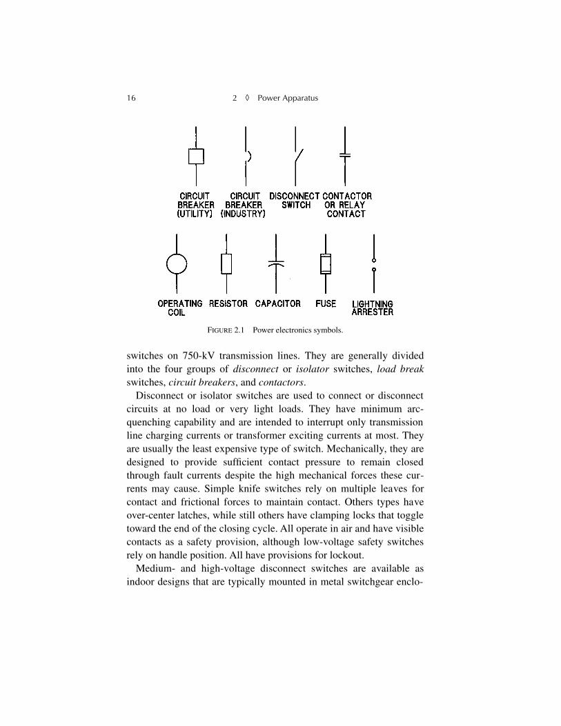
Commonly used symbols in power electronics diagrams are shownin Fig. 2.1. The utility breaker symbol is generally used in single linedrawings of power sources, whereas the industrial symbol is used onschematics. There are no hard and fast rules, however, and there are anumber of variations on this symbol set.
2.1. Switchgear
The equipments intended to connect and disconnect power circuits areknown collectively as
switchgear
(please—not
switchgears
and not
switch-gear
). Switchgear units range from the small, molded-case cir-cuit breakers in a household panelboard to the huge, air break
16 2
◊
Power Apparatus
switches on 750-kV transmission lines. They are generally dividedinto the four groups of
disconnect
or
isolator
switches,
load break
switches,
circuit breakers
, and
contactors
.Disconnect or isolator switches are used to connect or disconnect
circuits at no load or very light loads. They have minimum arc-quenching capability and are intended to interrupt only transmissionline charging currents or transformer exciting currents at most. Theyare usually the least expensive type of switch. Mechanically, they aredesigned to provide sufficient contact pressure to remain closedthrough fault currents despite the high mechanical forces these cur-rents may cause. Simple knife switches rely on multiple leaves forcontact and frictional forces to maintain contact. Others types haveover-center latches, while still others have clamping locks that toggletoward the end of the closing cycle. All operate in air and have visiblecontacts as a safety provision, although low-voltage safety switchesrely on handle position. All have provisions for lockout.
Medium- and high-voltage disconnect switches are available asindoor designs that are typically mounted in metal switchgear enclo-
FIGURE 2.1 Power electronics symbols.
2.1. Switchgear 17
sures or as outdoor switches incorporated into elevated structures.Both horizontally and vertically operating switches are available inoutdoor designs, and most are available with motor operators. Somehave optional pneumatic operators.
Load break switches generally follow the basic design arrange-ments of disconnect switches except that they are equipped with arcchutes that enable them to interrupt the current they are designed tocarry. They are not designed to interrupt fault currents; they mustremain closed through faults. Again, motor operators are available inmost designs. Motor-operated load break switches can be a lower-costalternative to circuit breakers in some applications where remote con-trol is required.
Circuit breakers are the heavy-duty members of the switchgear fam-ily. They are rated thermally for a given continuous load current aswell as a maximum fault current that they can interrupt. The arcingcontacts are in air with small breakers, but the larger types have con-tacts in a vacuum or in oil. High-voltage utility breakers may utilizesulfur hexafluoride (SF
6
) gas. Most breakers have a stored energyoperating mechanism in which a heavy spring is wound up by a motorand maintained in a charged state. The spring energy then swiftlyparts the contacts on a trip operation. Typically, the circuit is clearedin 3 to 5 cycles, since rapid interruption is essential to minimize archeating and contact erosion. Indoor breakers are usually in metal cab-inets as part of a switchgear lineup, whereas outdoor breakers may bestand-alone units.
Some caution should be used when specifying vacuum circuitbreakers. When these breakers interrupt an arc, the voltage across thecontacts is initially quite low. As the current drops to a low value,however, it is suddenly extinguished with a very high
di/dt
. This cur-rent is termed the
chop current
, and it can be as high as 3 to 5 A. If thebreaker is ahead of a transformer, the high
di/dt
level can generate ahigh voltage through the exciting inductance of the transformer, andthis can be passed on to secondary circuits. The required voltage con-trol can be obtained with arresters on the primary or metal oxide
18 2
◊
Power Apparatus
varistors (MOVs) on the secondary of the transformer. The MOVshould be rated to dissipate the transformed chop current at theclamping voltage rating of the MOV. It also must be rated forrepeated operations while dissipating the 1/2 LI
2
energy of the pri-mary inductance where I is the chop current.
Molded case breakers are equipped with thermal and magneticoverload elements that are self-contained. They are rated by maxi-mum load current and interrupt capacity. Thermal types employselectable heaters to match the load current for overload protection.Larger breakers are operated from external protective relays that canprovide both overload and short circuit protection through time over-current elements and instantaneous elements. Nearly all relays areoperated from current transformers and most are now solid-state.
Because of their heavy operating mechanisms, circuit breakers arenot rated for frequent operation. Most carry a maximum number ofrecommended operations before being inspected and repaired if nec-essary. Also, after clearing a fault, breakers should be inspected forarc damage or any mechanical problems.
The real workhorses of switchgear are the contactors. These areelectromagnetically operated switches that can be used for motorstarting and general-purpose control. They are rated for many thou-sands of operations. Contactors can employ air breaks at low voltagesor vacuum contacts at medium voltages. Most have continuouslyenergized operating coils and open when control power is removed.Motor starters can handle overloads of five times rated or more, andlighting contactors also have overload ratings for incandescent lamps.The operating coils often have a magnetic circuit with a large air gapwhen open and a very small gap when closed. The operating coilsmay have a high inrush current when energized, and the control powersource must be able to supply this current without excessive voltagedrop. Some types have optional DC coils that use a contact to insert acurrent reducing resistor into the control circuit as the contactorcloses.
2.2. Surge Suppression 19
Any piece of electrically operated switchgear, whether breaker orcontactor, has inductive control circuits that can develop high volt-ages in control circuits when interrupted. Good design practice callsfor R/C transient suppressors on operating coils or motors. MOVswill limit the developed voltage on opening but will be of no help inlimiting the
di/dt
that may interfere with other circuits. Contactorsmay be mounted within equipment cabinets or as standalone items.
2.2. Surge Suppression
Transient overvoltages can arise from a number of sources. Power dis-turbances result from lightning strokes or switching operations ontransmission and distribution lines. Switching of power factor correc-tion capacitors for voltage control is a major cause of switching tran-sients. All utility lines are designed for a certain
basic insulation level(BIL)
that defines the maximum surge voltage that will not damagethe utility equipment but which may be passed on to the customer.Some consideration should be given to the supply system BIL in high-power electronics with direct exposure to medium-voltage utilitylines. Such information is generally available from the utility repre-sentative. The standard test waveform for establishing BIL capabilityis a voltage that rises to the instantaneous BIL value in 1.2 µs anddecays to half that value in another 50 µs.
Other sources of transient overvoltages may lie within power elec-tronics equipment itself. Interrupting contactor coils has already beenmentioned. Diode and SCR reverse recovery current transients canalso propagate within equipment. Arcing loads may require shieldingof control circuits. In general, a solid grounding system will minimizeproblems.
Apparatus for surge protection covers the range from the little discsin 120-V power strips for computers to the giant lightning arresters on765-kV transmission lines. Many types now utilize the nonlinearcharacteristics of MOVs. These ZnO ceramic elements have a low
20 2
◊
Power Apparatus
leakage current as the applied voltage is increased until a threshold isreached at which the current will increase rapidly for higher voltages.The operating voltage is controlled by the thickness of the ceramicdisk and the processing. MOVs may be stacked in series for highervoltages and in parallel for higher currents.
Lightning arresters are classified by their current rating at a givenclamping voltage. Station-class arresters can handle the highest cur-rents and are the type used by utilities on transmission and subtrans-mission lines. Intermediate-class arresters have a lesser clampingability and are used on substations and some power electronics thatare directly connected to a substation. The lowest clamping currentsare in distribution-class arresters that are used on distribution feedersand the smaller power electronics equipment. The cost, of course, isrelated to the clamping current. Arresters are rated for their clampingvoltage by class and for their
maximum continuous operating voltage,MCOV.
They are typically connected line-to-ground. Lightning arrest-ers are often used to protect dry-type transformers in power electronicequipment, because such transformers may have a lower BIL ratingthan the supply switchgear. In 15-kV-class equipment, for example,the switchgear may be rated for 95 or 110 kV BIL, whereas the trans-former may be rated for only 60 kV.
As a design rule, MOVs used for the protection of power electronicswill limit peak voltage transients to 2 1/2 times their maximum con-tinuous rated rms voltage. They may be connected either line-to-lineor line-to-ground in three-phase circuits. Line-to-line connectionslimit switching voltage transients best but do not protect against com-mon-mode (all three lines to ground) transients. On the other hand,the line-to-ground connection that protects against common-modetransients does not do as good a job on applied line transients. Foroptimum protection in equipments with exposure to severe lightningor switching transients, both may be appropriate. The volt-amperecurves for a MOV should be checked to be sure the device can sinksufficient current at the maximum tolerable circuit voltage to handlethe expected transient energies. This current will be a function of the
2.3. Conductors 21
MOV size, and a wide range of diameters is available to handle nearlyany design need. Small units are supplied with wire leads, whereas thelarger units are packaged in molded cases with mounting feet andscrew terminals for connections.
Another device in the protection arsenal is the surge capacitor.Transient voltages with fast rise times, high dv/dt, may not distributethe voltage evenly among the turns on a transformer or motor wind-ing. This effect arises because of the turn-to-turn and turn-to-groundcapacitance distributions in the winding, an effect described in Chap-ter 7. Surge capacitors can be used to slow the dv/dt and minimize theovervoltages on the winding ends. These are generally in the range of0.5 to 1.0 µF for medium-voltage service. Some care should be exer-cised when these are used with SCR circuits because of the possibilityof serious overvoltages from ringing. Damping resistors may berequired.
2.3. Conductors
Current-carrying conductors range from the small wires of home cir-cuits to massive bus bar sets that may carry several hundred kiloam-peres. Copper is the primary conductor, with aluminum often used forbus bars and transformer windings. Conductor cross-sectional areasare designated by American Wire Gauge (AWG) number in thesmaller sizes, with a decrease of three numbers representing a dou-bling of the cross-sectional area. Numbered sizes go up to #0000, 4Ø(four aught). For larger conductors, the cross sections are expresseddirectly in circular mils, D
2
, where D is the conductor diameter inthousandths of an inch. For example, a conductor 1/2 inch in diameterwould be 250,000 circular mils. This would usually be expressed as250 kcm, although older tables may use 250 mcm. For noncircularconductors, the area in circular mils is the area in square inches times(4/
π
)
×
10
6
.High-current conductors are usually divided into a number of
spaced parallel bus bars to facilitate cooling. A rough guide to current
22 2
◊
Power Apparatus
capacity for usual conditions is 1000 A/in
2
of cross section. Connec-tions between bus bar sections should be designed to avoid problemsfrom differential expansion between the conductors and the bolts thatfasten them, as both heat up from current or ambient temperature. Sil-icon bronze bolts are a good match for the temperature coefficient ofexpansion of copper, and they have sufficient strength for good con-nections. However, highly reliable connections can be made betweencopper or aluminum bus sections with steel bolts and heavy Bellevillewashers on top of larger-diameter steel flat washers. The joint shouldbe tightened until the Belleville washer is just flat. Ordinary splitwashers are not recommended. If the bus is subjected to high mag-netic fields, stainless steel hardware should be used, but the field fromthe bus itself does not usually require this. Environmental conditions,however, may favor stainless.
All joints in buswork must be clean and free of grease. Joints can becleaned with fine steel wool and coated with a commercial joint com-pound before bolting. Aluminum bus must be cleaned free of all oxideand then immediately protected with an aluminum-rated joint com-pound to prevent oxide formation.
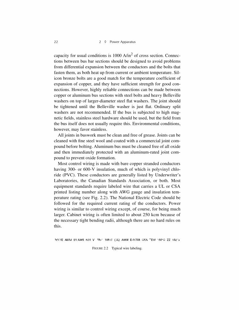
Most control wiring is made with bare copper stranded conductorshaving 300- or 600-V insulation, much of which is polyvinyl chlo-ride (PVC). These conductors are generally listed by Underwriter’sLaboratories, the Canadian Standards Association, or both. Mostequipment standards require labeled wire that carries a UL or CSAprinted listing number along with AWG gauge and insulation tem-perature rating (see Fig. 2.2). The National Electric Code should befollowed for the required current rating of the conductors. Powerwiring is similar to control wiring except, of course, for being muchlarger. Cabinet wiring is often limited to about 250 kcm because ofthe necessary tight bending radii, although there are no hard rules onthis.
FIGURE 2.2 Typical wire labeling.
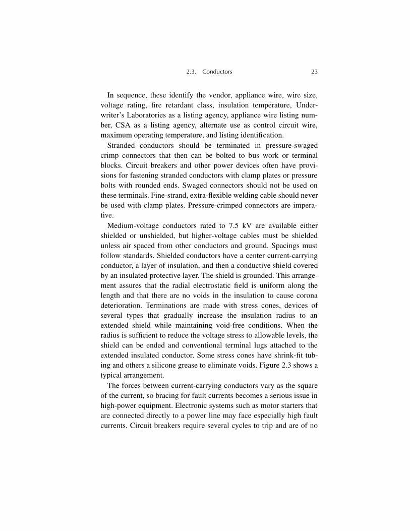
2.3. Conductors 23
In sequence, these identify the vendor, appliance wire, wire size,voltage rating, fire retardant class, insulation temperature, Under-writer’s Laboratories as a listing agency, appliance wire listing num-ber, CSA as a listing agency, alternate use as control circuit wire,maximum operating temperature, and listing identification.
Stranded conductors should be terminated in pressure-swagedcrimp connectors that then can be bolted to bus work or terminalblocks. Circuit breakers and other power devices often have provi-sions for fastening stranded conductors with clamp plates or pressurebolts with rounded ends. Swaged connectors should not be used onthese terminals. Fine-strand, extra-flexible welding cable should neverbe used with clamp plates. Pressure-crimped connectors are impera-tive.
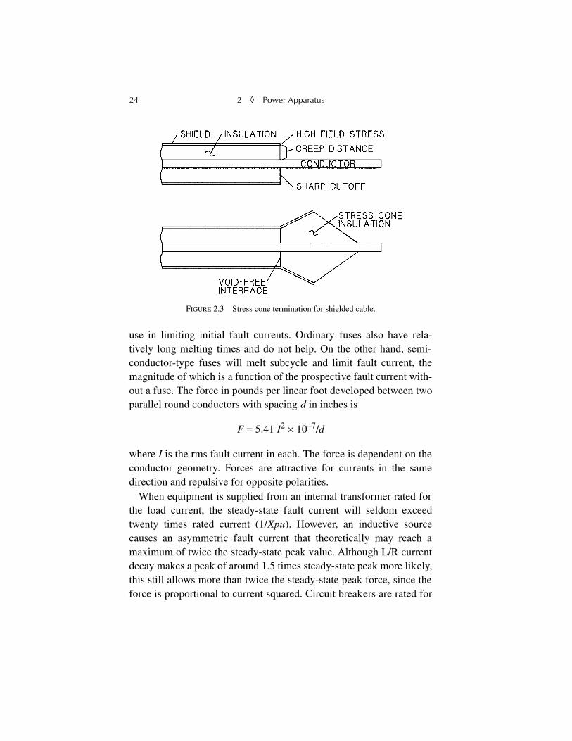
Medium-voltage conductors rated to 7.5 kV are available eithershielded or unshielded, but higher-voltage cables must be shieldedunless air spaced from other conductors and ground. Spacings mustfollow standards. Shielded conductors have a center current-carryingconductor, a layer of insulation, and then a conductive shield coveredby an insulated protective layer. The shield is grounded. This arrange-ment assures that the radial electrostatic field is uniform along thelength and that there are no voids in the insulation to cause coronadeterioration. Terminations are made with stress cones, devices ofseveral types that gradually increase the insulation radius to anextended shield while maintaining void-free conditions. When theradius is sufficient to reduce the voltage stress to allowable levels, theshield can be ended and conventional terminal lugs attached to theextended insulated conductor. Some stress cones have shrink-fit tub-ing and others a silicone grease to eliminate voids. Figure 2.3 shows atypical arrangement.
The forces between current-carrying conductors vary as the squareof the current, so bracing for fault currents becomes a serious issue inhigh-power equipment. Electronic systems such as motor starters thatare connected directly to a power line may face especially high faultcurrents. Circuit breakers require several cycles to trip and are of no
24 2
◊
Power Apparatus
use in limiting initial fault currents. Ordinary fuses also have rela-tively long melting times and do not help. On the other hand, semi-conductor-type fuses will melt subcycle and limit fault current, themagnitude of which is a function of the prospective fault current with-out a fuse. The force in pounds per linear foot developed between twoparallel round conductors with spacing
d
in inches is
F
= 5.41
I
2
×
10
–7
/
d
where
I
is the rms fault current in each. The force is dependent on theconductor geometry. Forces are attractive for currents in the samedirection and repulsive for opposite polarities.
When equipment is supplied from an internal transformer rated forthe load current, the steady-state fault current will seldom exceedtwenty times rated current (1/
Xpu
). However, an inductive sourcecauses an asymmetric fault current that theoretically may reach amaximum of twice the steady-state peak value. Although L/R currentdecay makes a peak of around 1.5 times steady-state peak more likely,this still allows more than twice the steady-state peak force, since theforce is proportional to current squared. Circuit breakers are rated for
FIGURE 2.3 Stress cone termination for shielded cable.
2.3. Capacitors 25
a maximum peak current that will allow them to close and latch themechanism.
High-current conductors are sometimes made with liquid cooling,one form utilizing copper tubing soldered or brazed into grooves thatare milled into the edge of the bus. An advantage of liquid cooling ingeneral is that most of the heat generated in the equipment can betransferred to the water, thus minimizing heating of the air in cabinetswith power electronics. Liquid cooling also saves on copper.
Buswork carrying high levels of AC currents, especially with a highharmonic content, may cause parasitic heating of adjacent steel cabi-net parts due to induced eddy currents. One solution to the problem isto replace the cabinet sections with stainless steel, aluminum, or fiber-glass sheet and structural members. Another solution is to interpose acopper plate between the bus and the offending cabinet member. Theplate will have high eddy currents, but the low resistance of the copperwill minimize losses. Eddy currents in the copper will generate a fluxin opposition to the incident flux to shield the cabinet steel.
2.4. Capacitors
The three major dielectric types of capacitors are those with varioustypes of film dielectrics used mostly for power factor correction andR/C snubbers, electrolytic types used for filters, and ceramic types inthe smaller ratings. The electrolytics have a much higher energy stor-age for a given volume, but they are not available in voltages aboveabout 500 V and are generally rated for DC service only. They furtherhave leakage currents and limited ratings for ripple current. Still, theirhigh energy density makes them popular for filters on DC power sup-plies. Even when operated at rated conditions, electrolytic capacitorshave a definite lifetime, because the electrolyte will evaporate overtime, especially if the capacitors are operated at high ripple currentsor in high ambient temperatures. Design consideration should begiven to adequate ventilation or heat sinking.
26 2
◊
Power Apparatus
Film dielectric power factor correction capacitors have replacedmost of the earlier types made with paper dielectric. These capacitorsare rated by kilovar (kvar) at rated voltage and are available both assingle units and three-phase assemblies in one can. Power factor cor-rection capacitors are always fused, either with standard medium-voltage fuses or with expulsion fuses in outdoor installations. The lat-ter discharge a plume of water vapor when ablative material in thefuse tube is evaporated as the fuse clears a fault.
Capacitors applied to a power system can create problems in thepresence of harmonics generated by nonlinear loads. The capacitorbank will form a parallel resonance with the source inductance of theutility supply, and if this resonance falls on a harmonic of the line fre-quency at which harmonic currents are present, the result can be seri-ous overvoltages and/or overcurrents. Good engineering practice is tomake a harmonic voltage survey before installing power factor correc-tion capacitors.
Power factor capacitor ratings are described in IEEE 18-2002,
IEEEStandard for Shunt Power Capacitors
. In summary, they may be oper-ated at maximum conditions of 110% rated rms voltage, 120% ofrated peak voltage, 135% of rated kvar, and 180% of rated rms cur-rent. Each of these ratings must include any harmonic voltages or cur-rents. When a capacitor is used with a series inductor to form a seriesresonant harmonic current trap, the increase in voltage at power fre-quency caused by the inductor must be considered. Most third-har-monic filters and some fifth-harmonic filters may require capacitorsrated above the nominal circuit voltage.
Energizing a section of a capacitor bank when the remainder of thebank is on line can result in damaging transient currents. When a sin-gle capacitor is connected to a power line, the surge current is limitedby the impedance of the source. Within a capacitor bank, however, theonly impedance limiting switching current is the small inductance andresistance of the buswork between sections. The charged capacitorswill discharge into the incoming capacitor with little current limiting.Each switched section within a capacitor bank should be protected
2.3. Capacitors 27
with a current-limiting reactor. Surge currents should be kept withinthe instantaneous ratings of the capacitors and switchgear.
Some capacitors designed for DC operation are made with a verylong sandwich of conductive and dielectric strips rolled into a cylin-der. Connections are made at one end of the two conductive strips, a“tab foil” design. Other types are made from a dielectric strip with afoil or deposited film of metal on one side. The film type can evapo-rate a small area of the metal on an internal failure without damage,and they are advertised as being self-healing. Capacitors designed forR/C snubber circuits, however, are often required to carry high rmscurrents and must be so rated. These capacitors are also formed from asandwich of aluminum foil strips and film dielectric rolled into a cyl-inder, but the foil layers are offset axially so that the connections tothe two foil windings can be made all along the two edges of thewinding. This arrangement, known as
extended foil
, lowers the induc-tance of the capacitor, and the resistive losses are much lower becausethe current does not have to flow in from one end of the winding,. Thetwo constructions are shown in Fig. 2.4. In general, DC-rated capaci-tors should not be used for AC service or R/C snubbers unless theyalso have an acceptable AC voltage and current rating. Note that snub-ber capacitors are subjected to repetitive charge and discharge that
FIGURE 2.4 Capacitor construction.
28 2
◊
Power Apparatus
results in much higher rms currents than would be expected from theircapacitance and applied voltage.
All capacitors can be connected in series or parallel for higher volt-ages or capacitances. They may be freely paralleled, but series con-nections may require the use of a voltage-sharing resistor connectedin parallel with each capacitor. Film types operated on AC circuitsmay not require sharing resistors for series operation, but resistors arerequired if DC voltage components are present. Without sharing resis-tors, the DC voltage will distribute in proportion to the highly variableleakage resistances. Sharing resistors must have a resistance lowenough to swamp out the leakage resistance variations to a sufficientdegree of voltage uniformity. Design guidance is available from ven-dors.
Yet another version of capacitors is the ceramic type. Made fromceramic material with a high dielectric constant, ceramic capacitorsgenerally have smaller capacitances but are available in high voltageratings. Such capacitors have a very low self-inductance and may bedesirable for some types of snubbers.
2.5. Resistors
Power electronic systems employ a large variety of resistor types andratings. At the low-power end, they are used in R/C snubber circuits,in voltage dividers, and as damping elements for various resonant cir-cuits. The two general resistor classes in the lower power ranges arewirewound and metallized film. Wirewound resistors are wound froma resistance alloy wire, usually on a cylindrical ceramic body. Termi-nal connections are welded at each end of a solenoidal winding. Non-inductive wirewound resistors are made with two paralleled windingswound in opposite directions around the body so that their magneticfields tend to cancel. Another construction technique is to wind theresistor from an elongated hairpin with the loop anchored to one endof the body and the leads brought out at the other end, the two wires
2.3. Resistors 29
being insulated from each other. There are many variations on thesebasic construction techniques. Resistors for snubber use, especiallywith fast switching semiconductors, must have an inductance as lowas possible to minimize transient voltages. Metallized film resistorsutilize a vacuum deposited resistance metal film on a ceramic sub-strate. Such metal film resistors have little transient heat storagecapacity and are not generally recommended for snubber use. Thesame is true for carbon film resistors. Carbon composition types arepreferred for low-power snubbers. These are made from a bulk carboncylinder within a ceramic tube.
Ceramic resistors are formed in various configurations from any ofa number of conductive ceramics. Metallized sections made by spray-ing a conductive metal onto the ceramic allow for terminal connec-tions. These resistors tend to have a low inherent inductance thatmakes them useful for snubbers. Some are housed in cast metal bodiesthat provide an insulated heat sink for power dissipation.
High-power resistors take on several forms, all of which aredesigned to permit efficient cooling (see Fig. 2.5). Some in the powerranges up to a few kilowatts are made with rectangular conductors ofresistance alloy wound into an air core cylinder with appropriate insu-lators and supports. Resistors with still higher power ratings are madefrom stamped sheet metal resistance alloys, sometimes stainless steel,assembled into stacks with series, parallel, or series/parallel connec-tions for the desired resistance. The general description is
grid resis-tor.
Iron grid castings preceded this type of construction, and suchresistors were often used for starting DC motors on trolley cars.
Water-cooled resistors are useful in equipment with water-cooledsemiconductors or for the manufacture of compact testing loads forpower electronic systems. Many are made from stainless steel ormonel tubing with water flowing inside. In going through such a resis-tor from end to end, the cooling water may be expected to rise 3.8°Cfor a dissipation of 1 kW with water flow at 1 gal/min. Exit water tem-perature should be kept below about 70°C to minimize leaching mate-rial from the resistor interior wall.
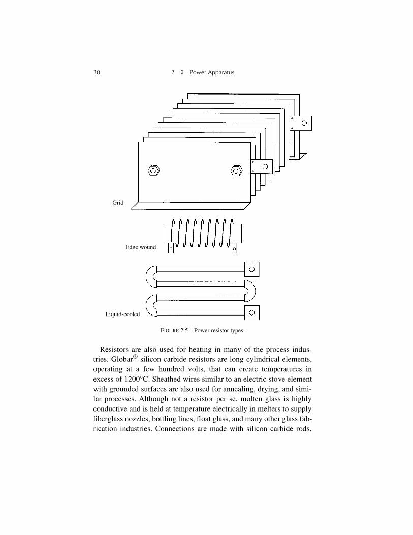
30 2
◊
Power Apparatus
Resistors are also used for heating in many of the process indus-tries. Globar
®
silicon carbide resistors are long cylindrical elements,operating at a few hundred volts, that can create temperatures inexcess of 1200°C. Sheathed wires similar to an electric stove elementwith grounded surfaces are also used for annealing, drying, and simi-lar processes. Although not a resistor per se, molten glass is highlyconductive and is held at temperature electrically in melters to supplyfiberglass nozzles, bottling lines, float glass, and many other glass fab-rication industries. Connections are made with silicon carbide rods.
FIGURE 2.5 Power resistor types.
Grid
Edge wound
Liquid-cooled
2.6. Fuses 31
Electric melters are more environmentally friendly than gas-firedunits.
2.6. Fuses
These protective elements are integral components of power electron-ics design. They range from the tiny glass cartridge fuses for controlcircuits to long, medium-voltage types. Each has characteristics thatare tailored for the particular applications. Control fuses should berated for about 125% of the expected load current. Standard types canbe used for most control circuits, but
slo-blo
fuses should be used forloads such as small motors and contactor coils that may draw inrushcurrents.
Semiconductor fuses are a special type that can limit the fault cur-rent by clearing subcycle, and they often protect power semiconduc-tors from load faults. Made with multiple thin, silver links embeddedin sand with a binder, they melt very quickly on faults and extinguishthe arc by evaporating the binder and melting the sand. They are avail-able in a wide range of currents, voltages, and case styles. Most have aceramic case, and many are designed to fit directly into buswork.Some high-current types are built as matched units, paralleled by thevendor. In pulsed applications, they should not be loaded with an rmspulse current more than 60 to 70% of the melting current for the pulseduration. Steady-state current should not exceed 80% of rated.
If protection of semiconductors is a design objective, the fuse I
2
trating should be well under the I
2
t rating of the semiconductor. Bettercoordination can be obtained in SCR converters if each SCR path isfused rather than the supply lines. This arrangement also offers pro-tection from internal bus-to-bus faults when the load can sourcepower.
Medium-voltage fuses are available as “E” rated for transformersand general-purpose applications, and “R” rated for use with applica-tions such as motors with high starting currents. Most mount in clip
32 2
◊
Power Apparatus
assemblies. These fuses may be matched in resistance and paralleledby the vendor for higher currents.
All high-current fuses should be bolted into sanded buswork withjoint compound and sufficient pressure to ensure a minimum resis-tance. Fuses are rated under the assumption that the buswork to whichthey are mounted will sink heat from the fuse and not source heat intoit.
2.7. Supply Voltages
The primary operating voltage for most power electronics is dividedinto two general classes: low-voltage, service voltages of 600 V orless, and medium-voltage, service voltages of 601 V through 34.5 kV.The vast majority of power electronics will wind up on either 600-V,5-kV, or 15-kV-class supplies in the U.S., but there are applications at2400 V and 6900 V, especially in older plants. Overseas, many othervoltages may be encountered, with 400 V, 3300 V, and 11 kV beingpopular, all at 50 Hz.
2.8. Enclosures
Equipment enclosures are described in NEMA standard ICS 1-110.Briefly, the designer may be expected to encounter Type 1, Type 4,and Type 12 enclosures most often. Type 1 is a general-purposeindoor, ventilated enclosure that protects personnel from accidentalexposure to high voltages and protects equipment from drippingwater. Type 4 is a watertight, dusttight, nonventilated indoor or out-door enclosure. Type 12 is a dusttight, driptight indoor enclosure.Type 12 may have nonventilated sections that are dusttight and venti-lated sections that are not.
Most enclosures are made with 10 to 12 ga steel, although smallerwall mount cabinets may be 14 ga. Corners and seams are welded,
2.9. Hipot, Corona, and BIL 33
and free-standing enclosures are equipped with three-point doorlatches. The rear wall of a cabinet has welded studs that support aremovable panel so that component assembly can be done outside thecabinet. All doors should be connected to the enclosure frame withflexible grounding straps for safety. The industry standard for freestanding enclosures is 90 inches in height.
2.9. Hipot, Corona, and BIL
Any insulation system must be able to tolerate a continually appliedvoltage, a transient overvoltage, and a surge voltage. Furthermore, itmust be free of partial discharge (corona) under the worst-case operat-ing conditions. The hipot test is typically a 1-min application of a 50-or 60-Hz voltage between all conductors and ground, during whichthe system must not fail shorted or show a fluctuating leakage current.There may, of course, be displacement currents from the capacitanceto ground.
Absent a specific high-potential test specification, a rule of thumb isa 1-min, 60-Hz applied sinusoidal voltage of twice rated rms voltageplus 1000 V for equipment rated 600 V or less and 2.25 times ratedvoltage plus 2000 V for ratings of 601 V and above.
The ability to withstand surge voltages is defined by a test wavewith a 1.2 µs rise time to peak and a 50 µs fall to half voltage. This testapproximately defines a basic insulation level (BIL) for the system.The test is a single application of this wave, and the requirement topass is simply freedom from breakdown.
Yet another test is the voltage at which a certain level of coronabegins. This is detected by the appearance of impulse discharge cur-rents on an oscilloscope as the applied voltage is slowly raised. Thevoltage at which these currents appear is the onset or inception level,and the cessation of the impulses as the voltage is reduced is the offsetor extinction voltage. Standardized metering circuits in commercialcorona testers allow these impulse currents to be quantified in micro-coulombs of current-time integral.
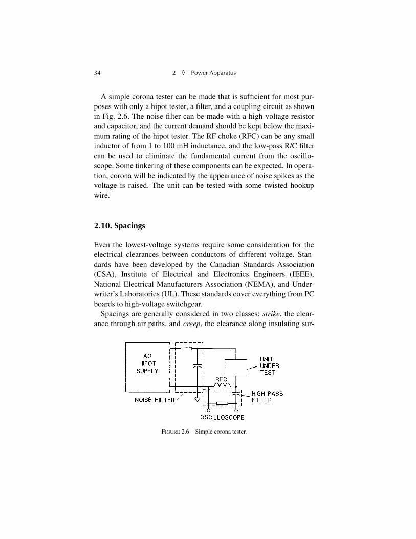
34 2
◊
Power Apparatus
A simple corona tester can be made that is sufficient for most pur-poses with only a hipot tester, a filter, and a coupling circuit as shownin Fig. 2.6. The noise filter can be made with a high-voltage resistorand capacitor, and the current demand should be kept below the maxi-mum rating of the hipot tester. The RF choke (RFC) can be any smallinductor of from 1 to 100 mH inductance, and the low-pass R/C filtercan be used to eliminate the fundamental current from the oscillo-scope. Some tinkering of these components can be expected. In opera-tion, corona will be indicated by the appearance of noise spikes as thevoltage is raised. The unit can be tested with some twisted hookupwire.
2.10. Spacings
Even the lowest-voltage systems require some consideration for theelectrical clearances between conductors of different voltage. Stan-dards have been developed by the Canadian Standards Association(CSA), Institute of Electrical and Electronics Engineers (IEEE),National Electrical Manufacturers Association (NEMA), and Under-writer’s Laboratories (UL). These standards cover everything from PCboards to high-voltage switchgear.
Spacings are generally considered in two classes:
strike
, the clear-ance through air paths, and
creep
, the clearance along insulating sur-
FIGURE 2.6 Simple corona tester.
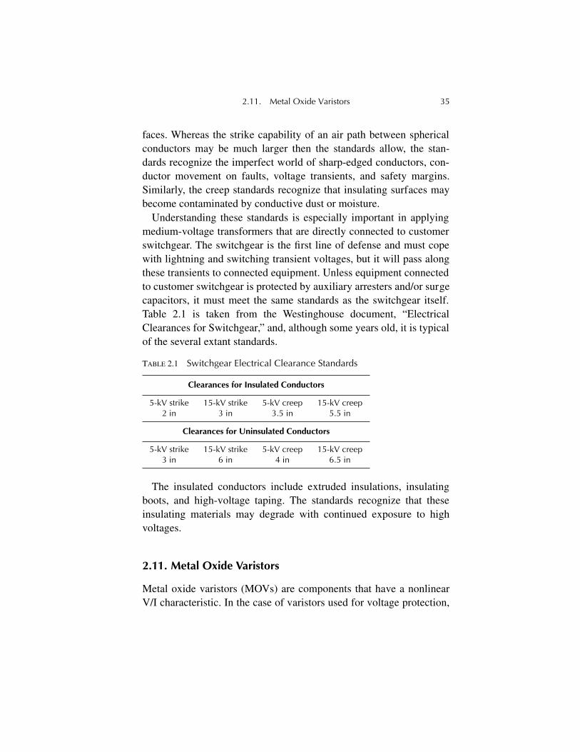
2.11. Metal Oxide Varistors 35
faces. Whereas the strike capability of an air path between sphericalconductors may be much larger then the standards allow, the stan-dards recognize the imperfect world of sharp-edged conductors, con-ductor movement on faults, voltage transients, and safety margins.Similarly, the creep standards recognize that insulating surfaces maybecome contaminated by conductive dust or moisture.
Understanding these standards is especially important in applyingmedium-voltage transformers that are directly connected to customerswitchgear. The switchgear is the first line of defense and must copewith lightning and switching transient voltages, but it will pass alongthese transients to connected equipment. Unless equipment connectedto customer switchgear is protected by auxiliary arresters and/or surgecapacitors, it must meet the same standards as the switchgear itself.Table 2.1 is taken from the Westinghouse document, “ElectricalClearances for Switchgear,” and, although some years old, it is typicalof the several extant standards.
The insulated conductors include extruded insulations, insulatingboots, and high-voltage taping. The standards recognize that theseinsulating materials may degrade with continued exposure to highvoltages.
2.11. Metal Oxide Varistors
Metal oxide varistors (MOVs) are components that have a nonlinearV/I characteristic. In the case of varistors used for voltage protection,
T
ABLE
2.1
Switchgear Electrical Clearance Standards
Clearances for Insulated Conductors
5-kV strike2 in
15-kV strike3 in
5-kV creep3.5 in
15-kV creep5.5 in
Clearances for Uninsulated Conductors
5-kV strike3 in
15-kV strike6 in
5-kV creep4 in
15-kV creep6.5 in
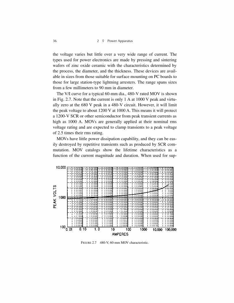
36 2
◊
Power Apparatus
the voltage varies but little over a very wide range of current. Thetypes used for power electronics are made by pressing and sinteringwafers of zinc oxide ceramic with the characteristics determined bythe process, the diameter, and the thickness. These devices are avail-able in sizes from those suitable for surface mounting on PC boards tothose for large station-type lightning arresters. The range spans sizesfrom a few millimeters to 90 mm in diameter.
The V/I curve for a typical 60-mm dia., 480-V rated MOV is shownin Fig. 2.7. Note that the current is only 1 A at 1000 V peak and virtu-ally zero at the 680 V peak in a 480-V circuit. However, it will limitthe peak voltage to about 1200 V at 1000 A. This means it will protecta 1200-V SCR or other semiconductor from peak transient currents ashigh as 1000 A. MOVs are generally applied at their nominal rmsvoltage rating and are expected to clamp transients to a peak voltageof 2.5 times their rms rating.
MOVs have little power dissipation capability, and they can be eas-ily destroyed by repetitive transients such as produced by SCR com-mutation. MOV catalogs show the lifetime characteristics as afunction of the current magnitude and duration. When used for sup-
FIGURE 2.7 480-V, 60-mm MOV characteristic.
2.11. Protective Relays 37
pressing breaker chop, for example, the maximum lifetime exposureshould be calculated so that a suitably sized MOV can be specified.
2.12. Protective Relays
Utilities and large industrial plants use a variety of relay types to pro-tect the system and its components against fault currents. The mostbasic types are overcurrent relays, which are available in a number ofstyles. All will trip a breaker on overcurrent, but the timing is widelyvariable among the several types. Relays are available from inverse toextremely inverse according to the design. All trip with a delay onlow-current faults but trip more quickly as the fault current rises.Many are available with an auxiliary instantaneous element that willtrip subcycle. Nearly all types are now electronic, with power derivedfrom the protected circuit itself. They are usually cascaded withdecreasing trip current settings as the system branches out fromsource to load through a succession of buses and circuit breakers. Thisallows an overcurrent to be cleared as close to the fault as possible soas to avoid disturbing other loads.
Another useful type is the differential relay. This relay has two setsof current coils and will trip on current imbalance between the twosets. When equipped with suitable current transformer ratios on thetwo sets, it can protect a transformer or generator from internal faultsand distinguish between them and external faults. Most differentialrelays have delay elements to allow for inrush currents in transform-ers.
Electric utilities often use impedance or distance relays to protecttransmission and distribution circuits. Although computers now takeover many of these tasks, the principle remains the same. The imped-ance relay has both current and voltage coils, with the voltage coilsused as restraint elements. If the voltage is high enough, the currentcoils are inhibited from tripping the associated breaker. In a sense, thisrelay measures the impedance and hence the distance to the fault, and
38 2 ◊ Power Apparatus
it can decide whether a downstream breaker can clear the fault withless disturbance to the system.
Relays are identified on system single-line diagrams as type 50 forinstantaneous overcurrent relays, 51 for time overcurrent relays, 64for ground fault relays, 87 for differential relays, and 21 for imped-ance or distance relays. The relay designations are usually shownadjacent to the circuit breaker they trip, with instantaneous and timeovercurrent relays shown as 50/51. Undervoltage, phase balance,phase sequence, directional power, and frequency relays are but a fewof the many other types available.
This essay has been a bit cavalier in equating, by implication,impedance to reactance. In most power systems work, the resistivelosses are small enough to have little effect on fault currents or regula-tion, so impedance is often considered as reactance in calculations.The same is true of commutation in converters where resistance doesplay a small role.
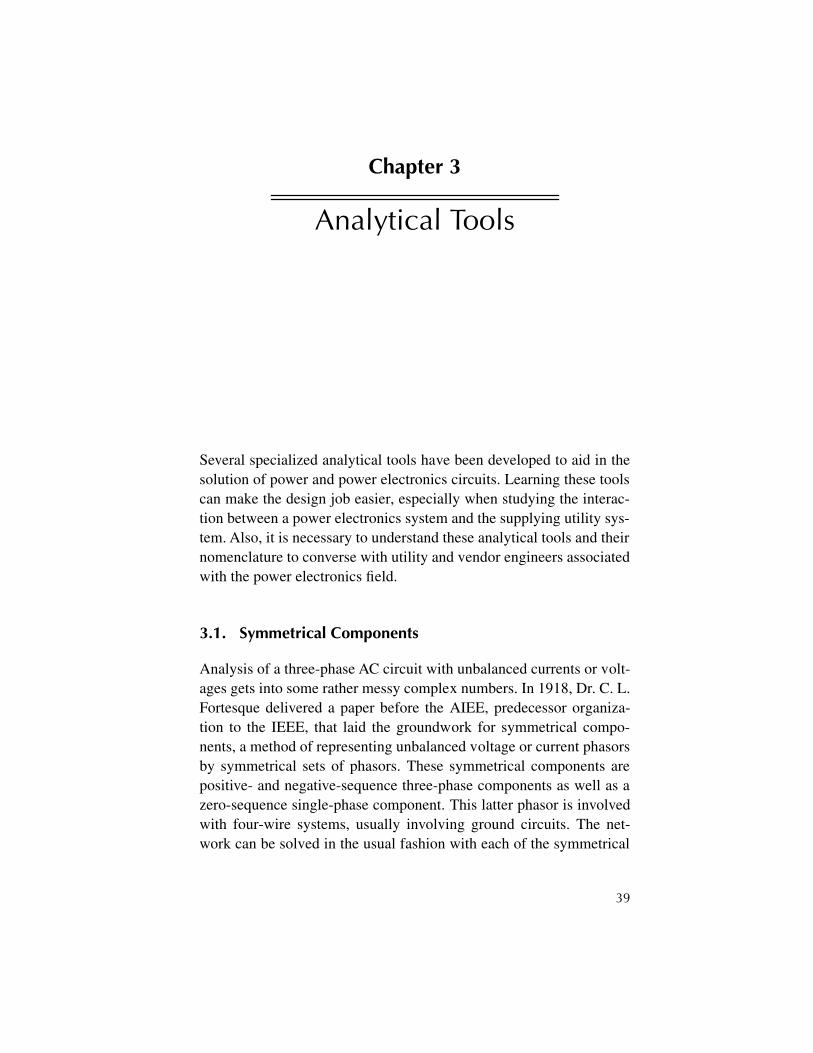
39
Chapter 3
Analytical Tools
Several specialized analytical tools have been developed to aid in thesolution of power and power electronics circuits. Learning these toolscan make the design job easier, especially when studying the interac-tion between a power electronics system and the supplying utility sys-tem. Also, it is necessary to understand these analytical tools and theirnomenclature to converse with utility and vendor engineers associatedwith the power electronics field.
3.1. Symmetrical Components
Analysis of a three-phase AC circuit with unbalanced currents or volt-ages gets into some rather messy complex numbers. In 1918, Dr. C. L.Fortesque delivered a paper before the AIEE, predecessor organiza-tion to the IEEE, that laid the groundwork for symmetrical compo-nents, a method of representing unbalanced voltage or current phasorsby symmetrical sets of phasors. These symmetrical components arepositive- and negative-sequence three-phase components as well as azero-sequence single-phase component. This latter phasor is involvedwith four-wire systems, usually involving ground circuits. The net-work can be solved in the usual fashion with each of the symmetrical
40 3
◊
Analytical Tools
components, and then the individual solutions combined to representthe unbalanced system. Symmetrical components are universally usedby power company engineers for system parameters.
Symmetrical component analysis uses a complex operator,
a
, where
a
= –0.5 +
j
0.866, a unit phasor at 120°. Then,
a
2
= –0.5 –
j
0.866, and
a
3
= 1.0. If a set of asymmetric phasors are given as
x
,
y
, and
z
, then
where all quantities are phasors.
Ex
0,
Ex
1, and
Ex
2 are referred to asthe zero-sequence, positive-sequence, and negative-sequence com-ponents of
x,
respectively. Then,
Ex
0 =
Ey
0 =
Ez
0,
Ey
1 =
a
2
Ex
1,
Ez
1 =
a
Ex
1,
Ey
2 =
a
Ex
2 and
Ez
2 =
a
2
Ex
2. This process is shown in Fig. 3.8 where a (very) unbalanced set of
phasors are
x
= 6.0,
y
= –
j
2.0 and
z
= –0.707 +
j
0.707. The sequencenetworks are shown at the right. In this case,
Ex
0 = 1.764 –
j
0.431
Ex
1 = 2.899 +
j
0.419
Ex
2 = 1.337 +
j
0.011
The original asymmetric phasors may then be reconstituted as
x
=
Ex
0 +
Ex
1 +
Ex
2
y
=
Ey
0 +
Ey
1 +
Ey
2 =
Ex
0 +
a
2
Ex
1 +
a
Ex
2
z
=
Ez
0 +
Ez
1 +
Ez
2 =
Ex
0 +
a
Ex
1 +
a
2
Ex
2
Ex0 x y z+ +( )3
-------------------------=
Ex1 x ay a2z++
3------------------------------=
Ex2 x a2y az+ +
3------------------------------=
3.2. Per Unit Constants 41
If the set of phasors just resolved were to represent load imped-ances, the line currents could be determined by impressing the bal-anced line voltages onto the three sequence networks separately andadding the three components of each line current.
Symmetrical components are often used to describe the characteris-tics of overhead transmission lines. For example, the familiar set ofthree conductors in a horizontal row has equal couplings from the twoouter lines to the center line, but they have a different coupling to eachother. Hence, the mutual inductances and capacitances of the set aredifferent. The use of symmetrical components of these impedancesallows the line to be analyzed as two balanced positive- and negative-sequence networks. The resultant currents can then be combined.Absent a grounded circuit, the zero-sequence network is not present.
The many circuit simulation software packages now available canreduce the need for using symmetrical components for circuit solu-tions, but they are still valuable for defining the unbalanced loadingand fault performances of synchronous machines.
3.2. Per Unit Constants
Per unit quantities greatly simplify comparisons between items ofpower apparatus and aid in solving fault calculations. Per unit is amethod of normalizing the characteristics of elements in a power elec-tronics system so they can be represented independent of the particu-lar voltage at that point in the system. Their characteristics are
FIGURE 3.1 Symmetrical components.
42 3
◊
Analytical Tools
translated relative to a common base so that extended calculations canbe made easily.
In its simplest form, a per unit quantity is merely the percent quan-tity divided by 100. It spares one the nonsense of 50% voltage times50% current equals 2500% power. In per unit notation, 0.5 pu voltagetimes 0.5 pu current equals 0.25 pu power as it should be. A trans-former with 6% impedance would have a per unit impedance of0.06 pu. Although not described as such, this impedance is based onthe rated voltage and current of the transformer. It accommodates thedifferences in primary and secondary voltages by describing the per-cent rated voltage in either winding required to produce rated currentin that winding with the other winding shorted. The regulation charac-teristics of the transformer are completely described by this figure.When other elements are added to a system, however, there will be awhole set of different ratings of the various elements. A 500-kVAtransformer at 4160 V with 6% reactance may serve a 50-kVA trans-former at 480 V with 4% reactance that, in turn, serves a 5-kVA light-ing transformer at 120 V with 3% reactance. It is a real nuisance tochase the various voltages and currents back through the system tofind, for example, the short circuit current at the final transformer. Perunit quantities make it easy.
First, one must choose a particular power level as a base quantity.The selection is completely arbitrary but is usually related to the rat-ing of one of the component items. In this case, the 50-kVA trans-former will be used as the base, and its leakage impedance will be 4%on that base, 0.04 pu. To relate the 5-kVA lighting transformer to thisquantity, one simply multiplies the 5-kVA impedance of 0.03 pu on itsown base by the power ratio of 50 kVA/5 kVA = 10. With the two incascade, the total impedance is now 0.04 + 0.03
×
10 = 0.34 pu. The500-kVA transformer by the same procedure becomes 0.06
50/500 =0.006 pu on the 50-kVA base. The series string impedance is then0.006 + 0.04 + 0.30 = 0.346 pu on the 50 kVA base. This total seriesimpedance is 0.0346 pu on a 5-kVA base, and a fault on the secondaryof the 5-kVA transformer will result in 1/0.0346 = 28.9 times rated
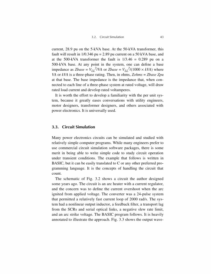
3.2. Circuit Simulation 43
current, 28.9 pu on the 5-kVA base. At the 50-kVA transformer, thisfault will result in 1/0.346 pu = 2.89 pu current on a 50 kVA base, andat the 500-kVA transformer the fault is 1/3.46 = 0.289 pu on a500-kVA base. At any point in the system, one can define a baseimpedance as
Zbase
=
V
LL
2
/
VA
or
Zbase
=
V
LL2
/(1000
×
kVA) whereVA or kVA is a three-phase rating. Then, in ohms, Zohms = Zbase Zpuat that base. The base impedance is the impedance that, when con-nected to each line of a three-phase system at rated voltage, will drawrated load current and develop rated voltamperes.
It is worth the effort to develop a familiarity with the per unit sys-tem, because it greatly eases conversations with utility engineers,motor designers, transformer designers, and others associated withpower electronics. It is universally used.
3.3. Circuit Simulation
Many power electronics circuits can be simulated and studied withrelatively simple computer programs. While many engineers prefer touse commercial circuit simulation software packages, there is somemerit in being able to write simple code to study circuit operationunder transient conditions. The example that follows is written inBASIC, but it can be easily translated to C or any other preferred pro-gramming language. It is the concepts of handling the circuit thatcount.
The schematic of Fig. 3.2 shows a circuit the author designedsome years ago. The circuit is an arc heater with a current regulator,and the concern was to define the current overshoot when the arcignited from applied voltage. The converter was a 24-pulse systemthat permitted a relatively fast current loop of 2000 rad/s. The sys-tem had a nonlinear output inductor, a feedback filter, a transport lagfrom the SCRs and serial optical links, a negative slew rate limit,and an arc strike voltage. The BASIC program follows. It is heavilyannotated to illustrate the approach. Fig. 3.3 shows the output wave-
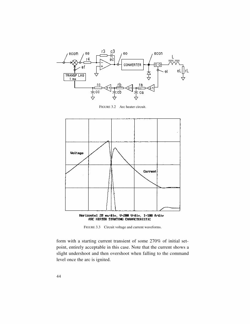
44
form with a starting current transient of some 270% of initial set-point, entirely acceptable in this case. Note that the current shows aslight undershoot and then overshoot when falling to the commandlevel once the arc is ignited.
FIGURE 3.2 Arc heater circuit.
FIGURE 3.3 Circuit voltage and current waveforms.

3.2. Circuit Simulation 45
3.3.1. Circuit Simulation Notes
Initial voltage: 0 – current integrator enabled at t = 0Initial current: 0.01 A (to get a finite inductance)Ignition voltage: 600 VEquivalent arc
resistance: 0.25 ΩInductor: Inductance inversely proportional to current to
1.1 power, bounded by 10 mH maximum and 1.1 mH minimum
Feedback: Three cascaded filter poles at 2000 rad/s. Filter will handle both feedback and anti-aliasing in the digital system.
Transport lag: 1 ms delay in SCRs and digital system, simulated as an actual delay
Regulator: Lead at 250 rad/s to match 4-ms load time con-stant
Negative slew rate: –10%/ms to approximate 50-Hz sine waveCommanded
current: 100 A, a low initial current setting to minimize overshoot
This program will run in BASIC 4.5 or higher as well asQuickBASIC.
'Arc heater starting programSCREEN 12 ' set 640 x 480 screenPALETTE 0,4144959 ' set reverse palette colorsPALETTE 15,0 'set background whiteDIM ed(10000)td = 100 'delay in 10 µs incrementsdt = .00001 ' time increment 10 µsicom = 100 ' current command levelecom = icom / 300 ' current command = .33 v for 100ArL = .25 ' load resistancer3 = 40000 ' lead resistorr4 = 10000 ' input resistor

46 3 ◊ Analytical Tools
ra = 500 ' filter resistorsrb = 500rc = 500 ca = .000001 ' filter capacitorscb = .000001cc = .000001 cd = .000001c3 = .000001 ' integrator capacitori = .01 ' initial currentagain: IF i <= 0 THEN i = 1 ' clip undershoot L = .01 * (250 / i ) ^ 1.1 ' inductor characteristicIF L > .01 THEN L = .01 ' maximum inductance 10 mHIF L < .0011 THEN L = .0011 ' minimum saturated
inductance 1.1 mHee = ecom - ef ' error signal of command minus
feedbackia = (ei - ea) / ra ' filter capacitor current for
Euler integrationib = (ea - eb) / rb ' same, next stageic = (eb - ec) / rc ' same, final stagep = n - td ' digital system transport lagIF p <1 THEN p = 1 ' initializeed(n) = ec ' last stage filter voltageef = ed(p) ' delay of td/100 msec = ec + ic * dt / cc ' three cascaded poles of filter
with poles at 2000 rad/seb = eb + ib * dt / cb ' sections are isolatedea = ea + ia * dt / ca ' Euler integrationei = .0033 * i ' 1500 A = 5 V feedback from shuntecon = 240 * eo ' converter gain, 5 v = 1200 VIF econ < 0 THEN econ = 0 ' commutating diode prevents
negative voltageIF econ > 1200 THEN econ = 1200 ' voltage ceilingIF (i < icom) AND (econ > 650) THEN econ = 650 '
starting voltage limitIF econx - econ > 1 THEN econ = econx - 1 ' negative
slew rate limit 10%/msi = i + (econ - eL) * dt / L ' load currentIF econ > 600 THEN k = 1 ' flag to detect first current
above isetpoint

3.4. Simulation Software 47
IF k = 0 THEN i = 0 ' no current until econ> 600 V arc ignition voltage
eL = i * rL ' load voltageeo = ee * ( r3 / r4 ) + ecap ' output voltage of opampIF eo > 10 THEN eo = 10 ' opamp limitecap = ecap + (eo - ecap ) / r3 * dt / c3 ' voltage on
integrator capPSET ( n / 20 + 50 , 400 - i ) ' plot currentPSET ( n / 20 + 50, 400 - .5 * econ ) ' plot voltagen = n + 1IF n > 10000 GOTO quit: ' end of displayeconx = econ ' set econx for prior voltage to set
negative slew rate maximumGOTO again:quit: FOR n = 0 to 400 STEP 100LINE ( 50 , n ) - ( 550 , n ) ' ordinate scaleNEXT FOR n = 50 to 550 STEP 100LINE (n , 0 ) - ( n , 400 ) ' abscissa scaleNEXT LOCATE 27 , 15: PRINT “ Horizontal 20 ms/div, V=200 V/
div, I=100 A/div”LOCATE 28 , 20: PRINT “ ARC HEATER STARTING
CHARTERISTIC”LOCATE 10,10: PRINT “Voltage”LOCATE 15,50: PRINT “Current”
3.4. Simulation Software
A number of software packages are now available to simulate theoperation of nearly any power electronic circuit. Component charac-teristics are included, and the programs are set up so that representa-tion of a circuit is relatively easy. All are described on the Internet insome detail, and most have student versions, limited-capability ver-sions, limited-time versions, or introductory packages. The commentsthat follow must be taken at a point in time, since the software evolvesrapidly.

48 3 ◊ Analytical Tools
MATLAB—An interactive program for numerical computation anddata visualization that is used by control engineers for analysis anddesign. Numerous “toolboxes” such as SIMULINK, a differentialequation solver, are available for simulation of dynamic systems. Itprovides an interactive graphical environment and a customizableset of block libraries that allow for the design, simulation, andimplementation of control, signal processing, communications, andother time-varying systems.
MATHCAD—An equation-based program that allows one to docu-ment, perform, and share calculation and design work. It can inte-grate mathematical notation, text, and graphics in a singleworksheet. It allows capture of the critical methods and values ofengineering projects.
Spice—One of the early simulation programs, Spice allows a circuitto be built directly on the display screen in schematic form. Librar-ies are available for the various circuit elements. Both steady-stateand transient behavior can be analyzed. Many related programs arealso available—PSpice, Saber, and Micro-Cap to name just a few.Some are directly compatible with Spice.
ElectroMagnetic Transients Program (EMTP)—Devoted primarily tothe solution of transient effects in electric power systems, variantsare available for circuit work. It is developed and maintained by aconsortium of international power companies and associated orga-nizations. The core program is in the public domain.
The above is only a sampling of the more popular software avail-able for circuit analysis. Most packages can be purchased on the Inter-net and some have student versions that can be downloaded at no cost.
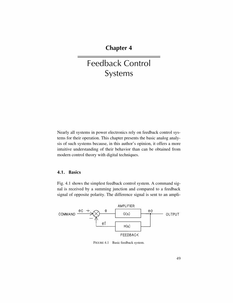
49
Chapter 4
Feedback Control Systems
Nearly all systems in power electronics rely on feedback control sys-tems for their operation. This chapter presents the basic analog analy-sis of such systems because, in this author’s opinion, it offers a moreintuitive understanding of their behavior than can be obtained frommodern control theory with digital techniques.
4.1. Basics
Fig. 4.1 shows the simplest feedback control system. A command sig-nal is received by a summing junction and compared to a feedbacksignal of opposite polarity. The difference signal is sent to an ampli-
FIGURE 4.1 Basic feedback system.
50 4
◊
Feedback Control Systems
fier that produces the system output with a feedback signal derivedfrom the amplifier output. Both the amplifier characteristic and thefeedback characteristic are functions of frequency and are shown asG(s) and H(s), respectively.
The performance of such system can be derived from an equationthat relates output to input. The equation is developed as follows:
1.
e
=
ec
–
ef
2.
eo
=
e
×
G(s)
3.
ef
=
eo
×
H(s)
4.
eo
=
G(s)
×
[
ec
–
eo
×
H(s)
]
5.
eo/ec
=
G(s)
/[1 +
G(s)
×
H(s
)] =
A
where
eo/ec
is the closed-loop system gain as a function of frequency.If the feedback is disconnected from the summing junction, then
A
=
G(s)
×
H(s)
, the open-loop gain. Simple systems such as the oneshown in Fig. 4.1 can be analyzed for stability and performance by anexamination of the open-loop gain characteristic as the frequency isvaried. For most purposes, the asymptotic response will suffice.
4.2. Amplitude Responses
Figure 4.2 shows the actual and asymptotic responses of a simple R/Ccircuit consisting of a series 1 M
Ω
resistor and a 3.3 µF shunt capaci-tor. Such frequency response characteristics for systems are referredto as
Bode (bodey) plots
. The plot is in decibels (dB) equal to 20
×
log
10
(
vo
/
vi
) where
vo
and
vi
are the output and input voltages, respectively. These may just aseasily be currents or currents translated to voltages through shunts orCTs. The asymptotic response is useful, because it can be quicklydrawn and has a maximum error of only 3 dB at the break point. Thebreak point in radians per second is simply the reciprocal of the timeconstant in seconds. Figure 4.3 shows a number of circuit elementsand their asymptotic frequency responses.
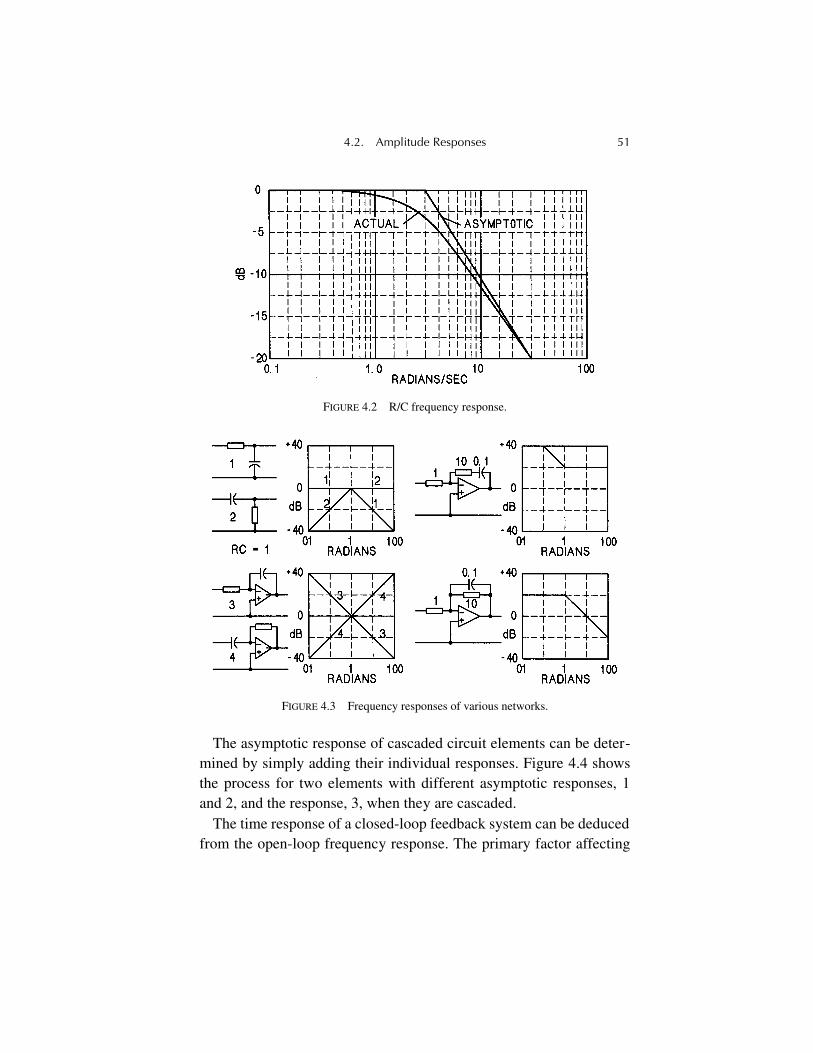
4.2. Amplitude Responses 51
The asymptotic response of cascaded circuit elements can be deter-mined by simply adding their individual responses. Figure 4.4 showsthe process for two elements with different asymptotic responses, 1and 2, and the response, 3, when they are cascaded.
The time response of a closed-loop feedback system can be deducedfrom the open-loop frequency response. The primary factor affecting
FIGURE 4.2 R/C frequency response.
FIGURE 4.3 Frequency responses of various networks.
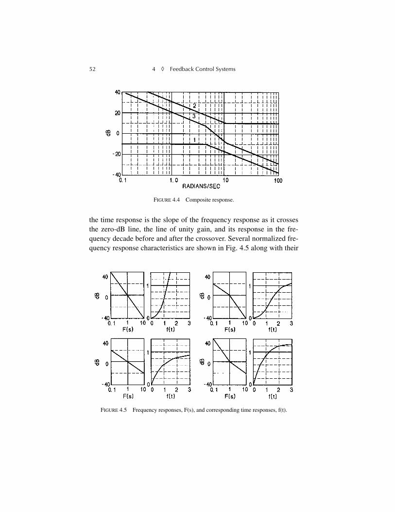
52 4
◊
Feedback Control Systems
the time response is the slope of the frequency response as it crossesthe zero-dB line, the line of unity gain, and its response in the fre-quency decade before and after the crossover. Several normalized fre-quency response characteristics are shown in Fig. 4.5 along with their
FIGURE 4.4 Composite response.
FIGURE 4.5 Frequency responses, F(s), and corresponding time responses, f(t).
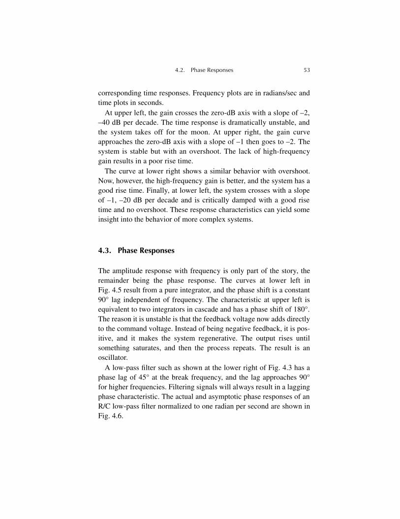
4.2. Phase Responses 53
corresponding time responses. Frequency plots are in radians/sec andtime plots in seconds.
At upper left, the gain crosses the zero-dB axis with a slope of –2,–40 dB per decade. The time response is dramatically unstable, andthe system takes off for the moon. At upper right, the gain curveapproaches the zero-dB axis with a slope of –1 then goes to –2. Thesystem is stable but with an overshoot. The lack of high-frequencygain results in a poor rise time.
The curve at lower right shows a similar behavior with overshoot.Now, however, the high-frequency gain is better, and the system has agood rise time. Finally, at lower left, the system crosses with a slopeof –1, –20 dB per decade and is critically damped with a good risetime and no overshoot. These response characteristics can yield someinsight into the behavior of more complex systems.
4.3. Phase Responses
The amplitude response with frequency is only part of the story, theremainder being the phase response. The curves at lower left inFig. 4.5 result from a pure integrator, and the phase shift is a constant90° lag independent of frequency. The characteristic at upper left isequivalent to two integrators in cascade and has a phase shift of 180°.The reason it is unstable is that the feedback voltage now adds directlyto the command voltage. Instead of being negative feedback, it is pos-itive, and it makes the system regenerative. The output rises untilsomething saturates, and then the process repeats. The result is anoscillator.
A low-pass filter such as shown at the lower right of Fig. 4.3 has aphase lag of 45° at the break frequency, and the lag approaches 90°for higher frequencies. Filtering signals will always result in a laggingphase characteristic. The actual and asymptotic phase responses of anR/C low-pass filter normalized to one radian per second are shown inFig. 4.6.
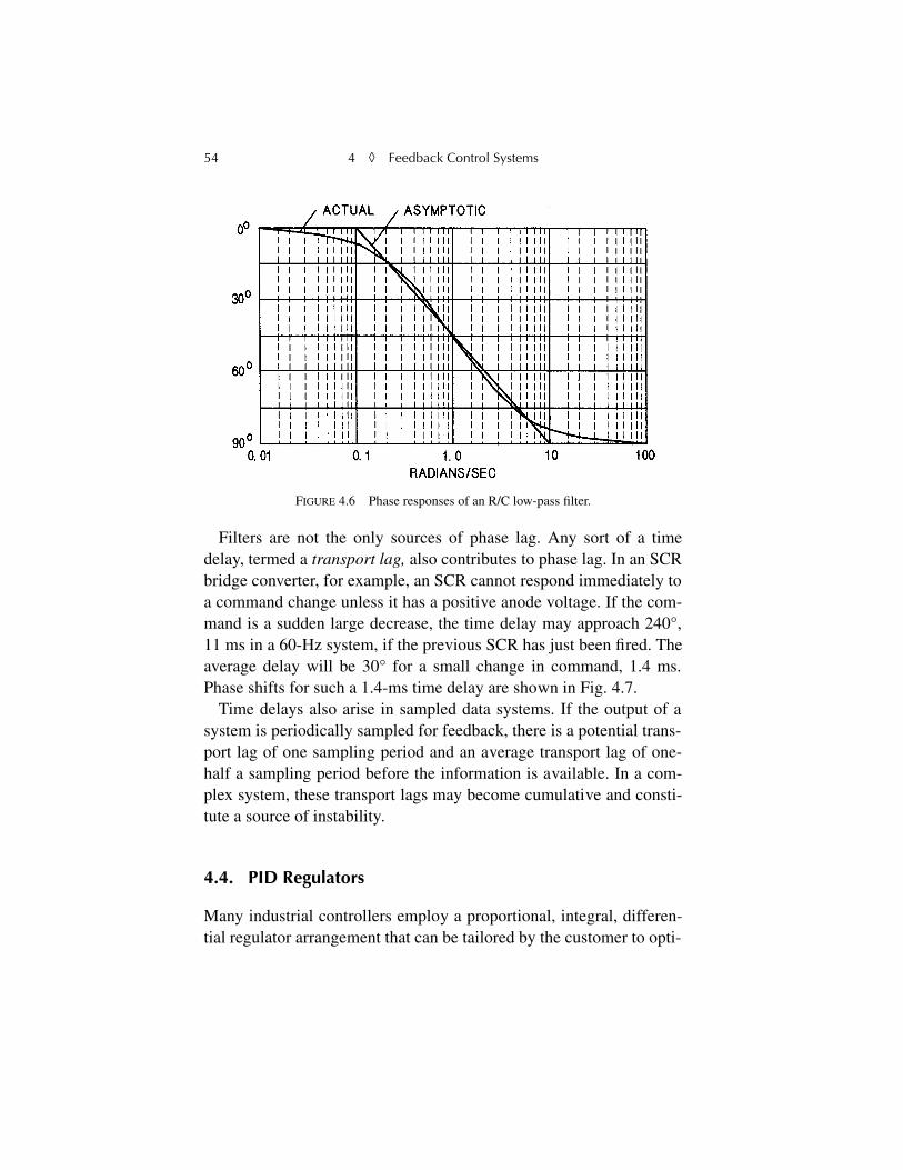
54 4
◊
Feedback Control Systems
Filters are not the only sources of phase lag. Any sort of a timedelay, termed a
transport lag,
also contributes to phase lag. In an SCRbridge converter, for example, an SCR cannot respond immediately toa command change unless it has a positive anode voltage. If the com-mand is a sudden large decrease, the time delay may approach 240°,11 ms in a 60-Hz system, if the previous SCR has just been fired. Theaverage delay will be 30° for a small change in command, 1.4 ms.Phase shifts for such a 1.4-ms time delay are shown in Fig. 4.7.
Time delays also arise in sampled data systems. If the output of asystem is periodically sampled for feedback, there is a potential trans-port lag of one sampling period and an average transport lag of one-half a sampling period before the information is available. In a com-plex system, these transport lags may become cumulative and consti-tute a source of instability.
4.4. PID Regulators
Many industrial controllers employ a proportional, integral, differen-tial regulator arrangement that can be tailored by the customer to opti-
FIGURE 4.6 Phase responses of an R/C low-pass filter.
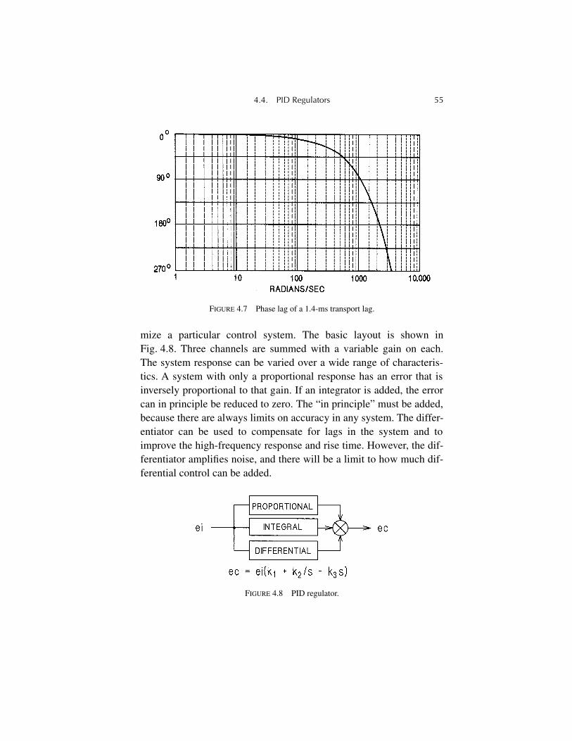
4.4. PID Regulators 55
mize a particular control system. The basic layout is shown inFig. 4.8. Three channels are summed with a variable gain on each.The system response can be varied over a wide range of characteris-tics. A system with only a proportional response has an error that isinversely proportional to that gain. If an integrator is added, the errorcan in principle be reduced to zero. The “in principle” must be added,because there are always limits on accuracy in any system. The differ-entiator can be used to compensate for lags in the system and toimprove the high-frequency response and rise time. However, the dif-ferentiator amplifies noise, and there will be a limit to how much dif-ferential control can be added.
FIGURE 4.7 Phase lag of a 1.4-ms transport lag.
FIGURE 4.8 PID regulator.
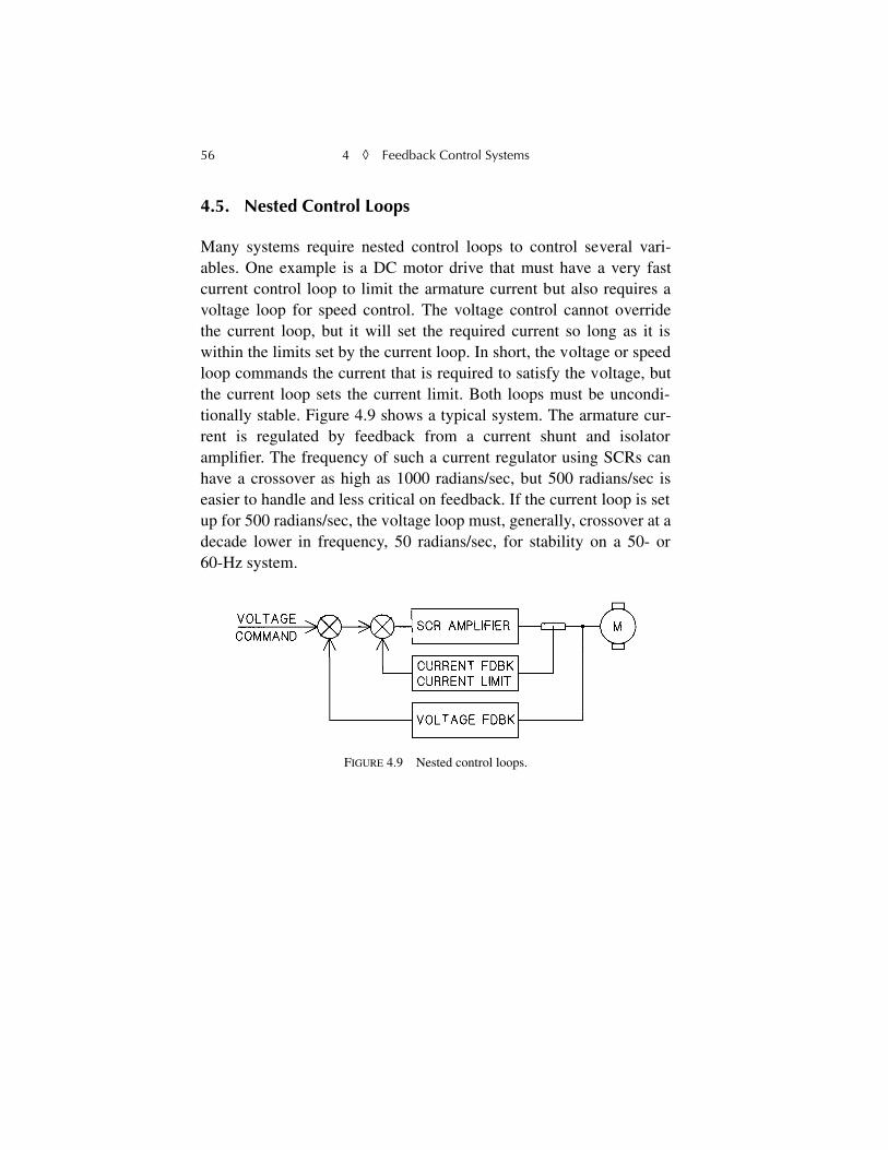
56 4
◊
Feedback Control Systems
4.5. Nested Control Loops
Many systems require nested control loops to control several vari-ables. One example is a DC motor drive that must have a very fastcurrent control loop to limit the armature current but also requires avoltage loop for speed control. The voltage control cannot overridethe current loop, but it will set the required current so long as it iswithin the limits set by the current loop. In short, the voltage or speedloop commands the current that is required to satisfy the voltage, butthe current loop sets the current limit. Both loops must be uncondi-tionally stable. Figure 4.9 shows a typical system. The armature cur-rent is regulated by feedback from a current shunt and isolatoramplifier. The frequency of such a current regulator using SCRs canhave a crossover as high as 1000 radians/sec, but 500 radians/sec iseasier to handle and less critical on feedback. If the current loop is setup for 500 radians/sec, the voltage loop must, generally, crossover at adecade lower in frequency, 50 radians/sec, for stability on a 50- or60-Hz system.
FIGURE 4.9 Nested control loops.
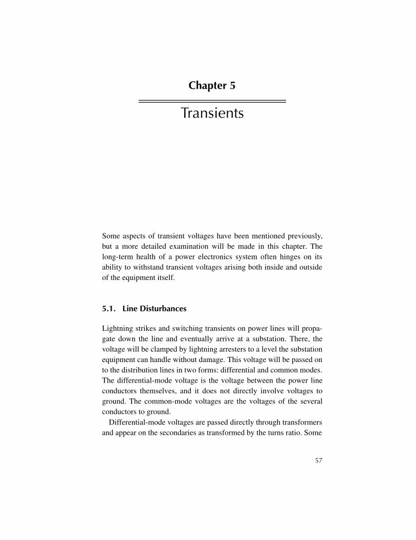
57
Chapter 5
Transients
Some aspects of transient voltages have been mentioned previously,but a more detailed examination will be made in this chapter. Thelong-term health of a power electronics system often hinges on itsability to withstand transient voltages arising both inside and outsideof the equipment itself.
5.1. Line Disturbances
Lightning strikes and switching transients on power lines will propa-gate down the line and eventually arrive at a substation. There, thevoltage will be clamped by lightning arresters to a level the substationequipment can handle without damage. This voltage will be passed onto the distribution lines in two forms: differential and common modes.The differential-mode voltage is the voltage between the power lineconductors themselves, and it does not directly involve voltages toground. The common-mode voltages are the voltages of the severalconductors to ground.
Differential-mode voltages are passed directly through transformersand appear on the secondaries as transformed by the turns ratio. Some
58 5
◊
Transients
attenuation may result from intrawinding capacitances, but interwind-ing capacitances may actually increase the voltage. Common-modevoltages are transferred to the secondary through the interwindingcapacitances and can be effectively stopped by an electrostatic shieldbetween the windings. Absent the shield, however, they can appear onthe secondaries with a magnitude close to that on the primary. Thiscan be a severe problem on medium-voltage systems where there isthe possibility of 10 kV or more being developed on secondaries toground.
The best protection from line-induced transients of all types on sec-ondaries is a set of MOVs. Line-to-line MOVs on the secondary arebest for differential-mode voltages, and line-to-ground MOVs willprovide the best protection from common-mode voltages if a shield isnot used. An electrostatic shield (Faraday screen) is a relatively low-cost addition to a transformer, and it is a good practice to specify ashield on transformers with medium-voltage primaries. With a shield,line-to-line MOVs are likely to provide sufficient transient protection.As mentioned in Chapter 3, dry-type transformers should be equippedwith at least distribution-class lightning arresters on medium-voltagecircuits.
5.2. Circuit Transients
Most gate drives for SCRs or insulated gate bipolar transistors(IGBTs) are supplied in one way or another through transformers withprimaries at control circuit potential and secondaries at the cathode oremitter voltage, which may be far above ground. The transformershave interwinding capacitances that will couple the power voltagetransients on the semiconductors to the low-voltage control circuits.Here, they may flow through printed circuit board traces and causeimproper operation or even component failure. The best protection isto equip the gate drive transformers with electrostatic shields and tobe sure their primaries are tied directly to ground whenever possible.
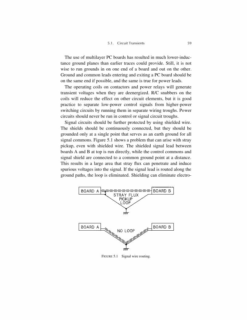
5.1. Circuit Transients 59
The use of multilayer PC boards has resulted in much lower-induc-tance ground planes than earlier traces could provide. Still, it is notwise to run grounds in on one end of a board and out on the other.Ground and common leads entering and exiting a PC board should beon the same end if possible, and the same is true for power leads.
The operating coils on contactors and power relays will generatetransient voltages when they are deenergized. R/C snubbers on thecoils will reduce the effect on other circuit elements, but it is goodpractice to separate low-power control signals from higher-powerswitching circuits by running them in separate wiring troughs. Powercircuits should never be run in control or signal circuit troughs.
Signal circuits should be further protected by using shielded wire.The shields should be continuously connected, but they should begrounded only at a single point that serves as an earth ground for allsignal commons. Figure 5.1 shows a problem that can arise with straypickup, even with shielded wire. The shielded signal lead betweenboards A and B at top is run directly, while the control commons andsignal shield are connected to a common ground point at a distance.This results in a large area that stray flux can penetrate and inducespurious voltages into the signal. If the signal lead is routed along theground paths, the loop is eliminated. Shielding can eliminate electro-
FIGURE 5.1 Signal wire routing.
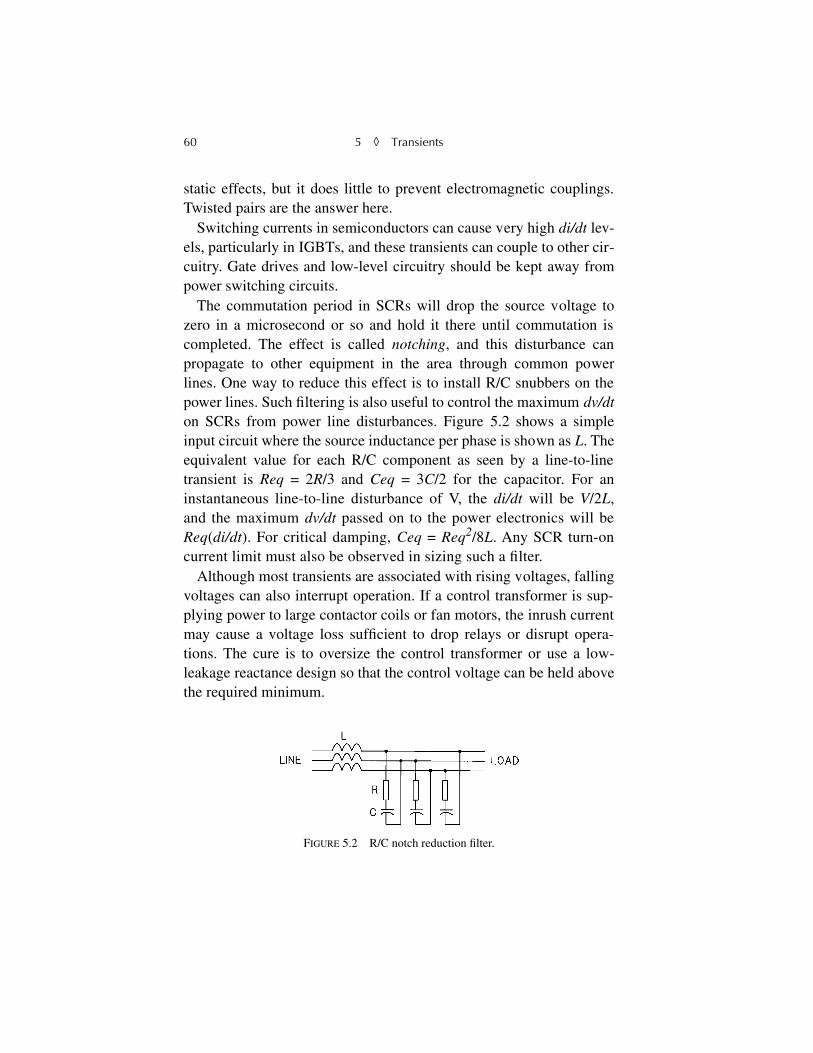
60 5
◊
Transients
static effects, but it does little to prevent electromagnetic couplings.Twisted pairs are the answer here.
Switching currents in semiconductors can cause very high
di/dt
lev-els, particularly in IGBTs, and these transients can couple to other cir-cuitry. Gate drives and low-level circuitry should be kept away frompower switching circuits.
The commutation period in SCRs will drop the source voltage tozero in a microsecond or so and hold it there until commutation iscompleted. The effect is called
notching
, and this disturbance canpropagate to other equipment in the area through common powerlines. One way to reduce this effect is to install R/C snubbers on thepower lines. Such filtering is also useful to control the maximum
dv/dt
on SCRs from power line disturbances. Figure 5.2 shows a simpleinput circuit where the source inductance per phase is shown as
L
. Theequivalent value for each R/C component as seen by a line-to-linetransient is
Req
= 2
R
/3 and
Ceq
= 3
C
/2 for the capacitor. For aninstantaneous line-to-line disturbance of V, the
di/dt
will be
V
/2
L
,and the maximum
dv/dt
passed on to the power electronics will be
Req
(
di/dt
). For critical damping,
Ceq
=
Req
2
/8
L
. Any SCR turn-oncurrent limit must also be observed in sizing such a filter.
Although most transients are associated with rising voltages, fallingvoltages can also interrupt operation. If a control transformer is sup-plying power to large contactor coils or fan motors, the inrush currentmay cause a voltage loss sufficient to drop relays or disrupt opera-tions. The cure is to oversize the control transformer or use a low-leakage reactance design so that the control voltage can be held abovethe required minimum.
FIGURE 5.2 R/C notch reduction filter.
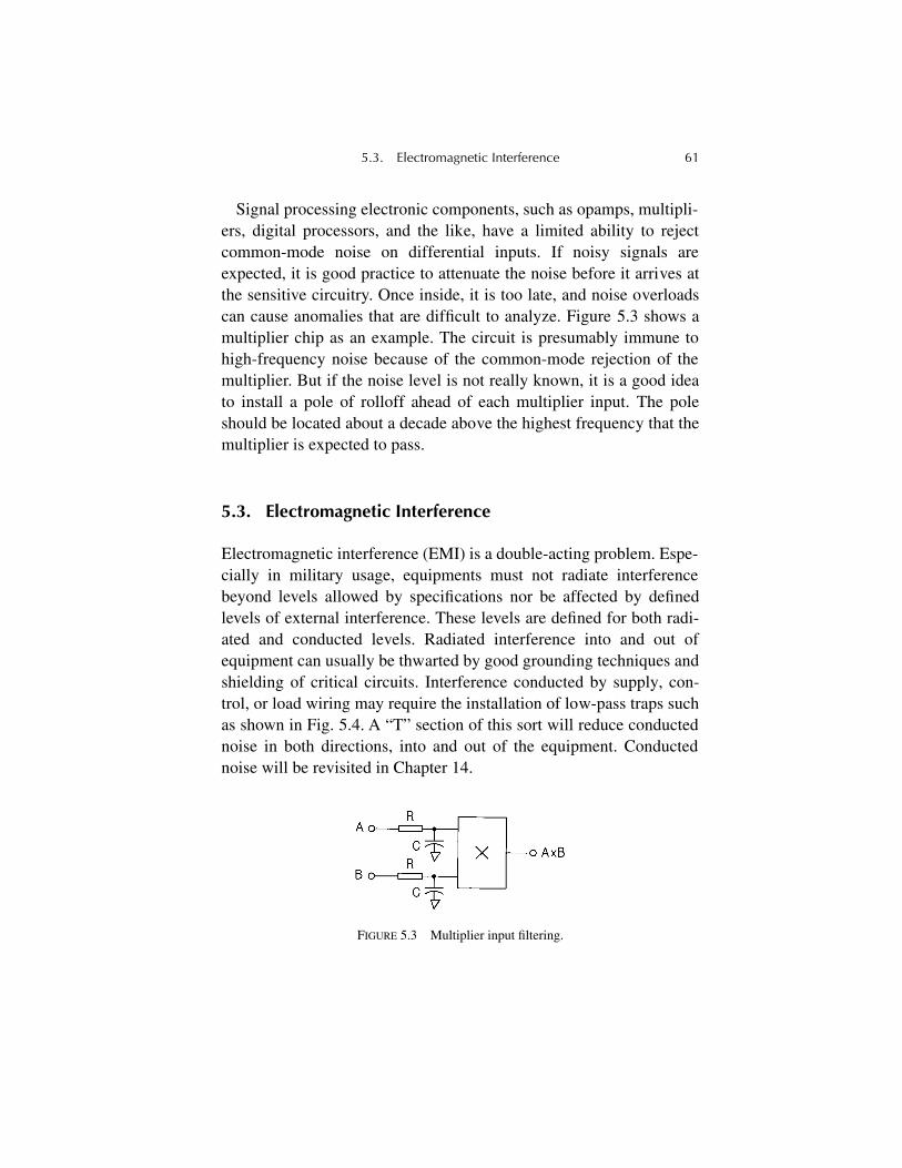
5.3. Electromagnetic Interference 61
Signal processing electronic components, such as opamps, multipli-ers, digital processors, and the like, have a limited ability to rejectcommon-mode noise on differential inputs. If noisy signals areexpected, it is good practice to attenuate the noise before it arrives atthe sensitive circuitry. Once inside, it is too late, and noise overloadscan cause anomalies that are difficult to analyze. Figure 5.3 shows amultiplier chip as an example. The circuit is presumably immune tohigh-frequency noise because of the common-mode rejection of themultiplier. But if the noise level is not really known, it is a good ideato install a pole of rolloff ahead of each multiplier input. The poleshould be located about a decade above the highest frequency that themultiplier is expected to pass.
5.3. Electromagnetic Interference
Electromagnetic interference (EMI) is a double-acting problem. Espe-cially in military usage, equipments must not radiate interferencebeyond levels allowed by specifications nor be affected by definedlevels of external interference. These levels are defined for both radi-ated and conducted levels. Radiated interference into and out ofequipment can usually be thwarted by good grounding techniques andshielding of critical circuits. Interference conducted by supply, con-trol, or load wiring may require the installation of low-pass traps suchas shown in Fig. 5.4. A “T” section of this sort will reduce conductednoise in both directions, into and out of the equipment. Conductednoise will be revisited in Chapter 14.
FIGURE 5.3 Multiplier input filtering.
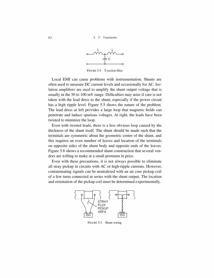
62 5
◊
Transients
Local EMI can cause problems with instrumentation. Shunts areoften used to measure DC current levels and occasionally for AC. Iso-lation amplifiers are used to amplify the shunt output voltage that isusually in the 50 to 100 mV range. Difficulties may arise if care is nottaken with the lead dress to the shunt, especially if the power circuithas a high ripple level. Figure 5.5 shows the nature of the problem.The lead dress at left provides a large loop that magnetic fields canpenetrate and induce spurious voltages. At right, the leads have beentwisted to minimize the loop.
Even with twisted leads, there is a less obvious loop caused by thethickness of the shunt itself. The shunt should be made such that theterminals are symmetric about the geometric center of the shunt, andthis requires an even number of leaves and location of the terminalson opposite sides of the shunt body and opposite ends of the leaves.Figure 5.6 shows a recommended shunt construction that several ven-dors are willing to make at a small premium in price.
Even with these precautions, it is not always possible to eliminateall stray pickup in circuits with AC or high-ripple currents. However,contaminating signals can be neutralized with an air core pickup coilof a few turns connected in series with the shunt output. The locationand orientation of the pickup coil must be determined experimentally.
FIGURE 5.4 T-section filter.
FIGURE 5.5 Shunt wiring.
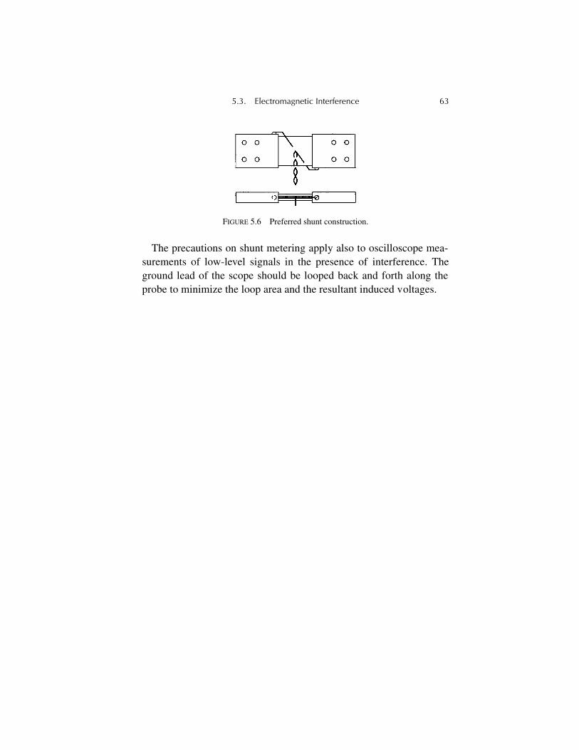
5.3. Electromagnetic Interference 63
The precautions on shunt metering apply also to oscilloscope mea-surements of low-level signals in the presence of interference. Theground lead of the scope should be looped back and forth along theprobe to minimize the loop area and the resultant induced voltages.
FIGURE 5.6 Preferred shunt construction.

65
Chapter 6
Traveling Waves
Traveling wave effects were once the nearly exclusive domain of com-munications engineers and electric utility transmission line engineers.However, as variable frequency, pulse width modulated (PWM) motordrives have gone to higher and higher PWM frequencies, standing-wave phenomena have appeared in motor circuits. Traveling wavesare now of concern to many power electronics engineers, and anunderstanding of their effects is necessary for motor protection ininstallations with long cables or high PWM frequencies. In modernterms, a transmission line is any set of parallel or coaxial conductorsof finite length, and they may be printed circuit conductors or miles ofoverhead wires.
6.1. Basics
Standing waves appear when a length of line is excited at a frequencyfor which the electrical line length is a significant part of an electricalwavelength. They result from the constructive and destructive inter-ference of forward and reflected waves on the line. The behavior ofthe line can be determined by solving the applicable differential equa-tions relating the line parameters to the exciting frequency. The solu-
66 6
◊
Traveling Waves
tion of the equations for a line with losses is rather complex and addslittle to the practical considerations, so the lossless line will be ana-lyzed instead.
In the lossless line,
L
is the series inductance per unit length, and
C
is the shunt capacitance. If a differential length,
dx
, is considered,the inductance for that length is
L
dx
, and the voltage in that length is
e
= –
L
dx
(
di/dt
). Since
e
= (
de/dx
)
dx
, the equation can be written as
dx
(
de/dx
) = –
L
dx
(
di/dt
). Similarly,
dx
(
di/dx
) = –
C
dx
(
de/dt
). Divid-ing out the
dx
terms and substituting partial derivatives, the funda-mental forms of transmission line equations result:
–
∂
e
/
∂
x
=
L
∂
i
/
∂
t
and –
∂
i
/
∂
/
x
=
C
∂
e
/
∂
t
By differentiating with respect to
x
and then with respect to
t
, theseequations can be solved simultaneously to yield second-order, ellipti-cal, partial differential equations for both
e
and
i
individually withrespect to
t
and
x
. The classical forms then result:
LC
∂
2
i
/
∂
t
2
–
∂
2
i
/
∂
x
2
= 0 and
LC
∂
2
e
/
∂
t
2
–
∂
2
e
/
∂
x
2
= 0
These equations can now be solved by transforms or classical meth-ods. Explicit solutions can be developed with hyperbolic functions inthe complex plane, and these solutions were the only practical meansof line analysis until the digital computer was developed. Fortunately,the computer offers an easier method of analysis by numerical inte-gration, and line losses can be incorporated with relative ease. Thedifference equations can be solved by simple Euler integration, so thewhole process is not nearly as daunting as in earlier years.
The difference equations for differential sections of line are shownin Fig. 6.1. These equations allow numerical solutions for the voltagesand currents on the line as functions of distance and time. Although itmay not be immediately apparent, these difference equations, in thelimit, replicate the differential equations.
Before proceeding to typical solutions, several derived parametersshould be defined. First, the line has a surge, or characteristic, imped-
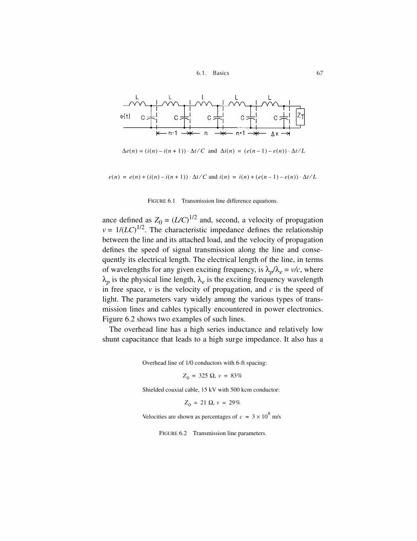
6.1. Basics 67
ance defined as
Z
0
= (
L/C
)
1/2
and, second, a velocity of propagation
v
= 1/(
LC
)
1/2
. The characteristic impedance defines the relationshipbetween the line and its attached load, and the velocity of propagationdefines the speed of signal transmission along the line and conse-quently its electrical length. The electrical length of the line, in termsof wavelengths for any given exciting frequency, is
λ
p
/
λ
e
=
v/c
, where
λ
p
is the physical line length,
λ
e
is the exciting frequency wavelengthin free space,
v
is the velocity of propagation, and
c
is the speed oflight. The parameters vary widely among the various types of trans-mission lines and cables typically encountered in power electronics.Figure 6.2 shows two examples of such lines.
The overhead line has a high series inductance and relatively lowshunt capacitance that leads to a high surge impedance. It also has a
FIGURE 6.1 Transmission line difference equations.
∆e n( ) i n( ) i n 1+( )–( )= ∆t C⁄⋅ and ∆i n( ) e n 1–( ) e n( )–( ) ∆t L⁄⋅=
e n( ) e n( ) i n( ) i n 1+( )–( )+ ∆t C⁄⋅ and i n( ) i n( ) e n 1–( ) e n( )–( )+ ∆t L⁄⋅= =
FIGURE 6.2 Transmission line parameters.
Overhead line of 1/0 conductors with 6-ft spacing:
Shielded coaxial cable, 15 kV with 500 kcm conductor:
Velocities are shown as percentages of
Z0 325 Ω, v 83%= =
Z0 21 Ω, v 29%= =
c 3 10× 8 m/s=
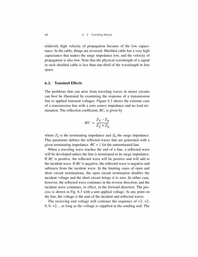
68 6 ◊ Traveling Waves
relatively high velocity of propagation because of the low capaci-tance. In the cable, things are reversed. Shielded cable has a very highcapacitance that makes the surge impedance low, and the velocity ofpropagation is also low. Note that the physical wavelength of a signalin such shielded cable is less than one-third of the wavelength in freespace.
6.2. Transient Effects
The problems that can arise from traveling waves in motor circuitscan best be illustrated by examining the response of a transmissionline to applied transient voltages. Figure 6.3 shows the extreme caseof a transmission line with a zero source impedance and no load ter-mination. The reflection coefficient, RC, is given by
where ZT is the terminating impedance and Z0 the surge impedance.This parameter defines the reflected waves that are generated with agiven terminating impedance. RC = 1 for the unterminated line.
When a traveling wave reaches the end of a line, a reflected wavewill be developed unless the line is terminated in its surge impedance.If RC is positive, the reflected wave will be positive and will add tothe incident wave. If RC is negative, the reflected wave is negative andsubtracts from the incident wave. In the limiting cases of open andshort circuit terminations, the open circuit termination doubles theincident voltage and the short circuit brings it to zero. In either case,however, the reflected wave continues in the reverse direction, and theincident wave continues, in effect, in the forward direction. The pro-cess is shown in Fig. 6.3 with a unit applied voltage. At any point onthe line, the voltage is the sum of the incident and reflected waves.
The receiving end voltage will continue the sequence of +2, +2,0, 0, +2… as long as the voltage is supplied at the sending end. The
RCZT Z0–
ZT Z0+-------------------=
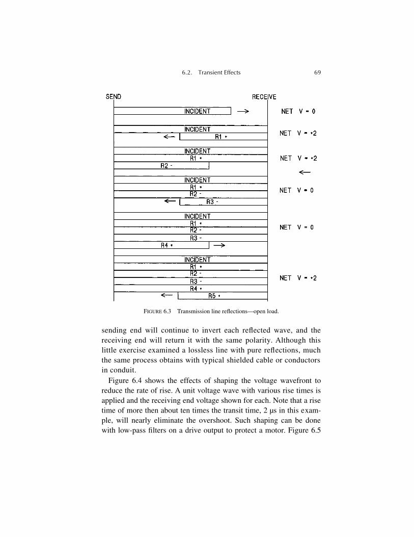
6.2. Transient Effects 69
sending end will continue to invert each reflected wave, and thereceiving end will return it with the same polarity. Although thislittle exercise examined a lossless line with pure reflections, muchthe same process obtains with typical shielded cable or conductorsin conduit.
Figure 6.4 shows the effects of shaping the voltage wavefront toreduce the rate of rise. A unit voltage wave with various rise times isapplied and the receiving end voltage shown for each. Note that a risetime of more then about ten times the transit time, 2 µs in this exam-ple, will nearly eliminate the overshoot. Such shaping can be donewith low-pass filters on a drive output to protect a motor. Figure 6.5
FIGURE 6.3 Transmission line reflections—open load.
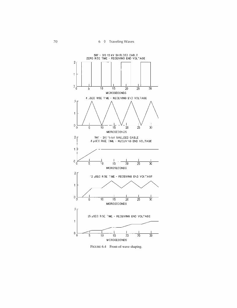
70 6 ◊ Traveling Waves
FIGURE 6.4 Front-of-wave shaping.
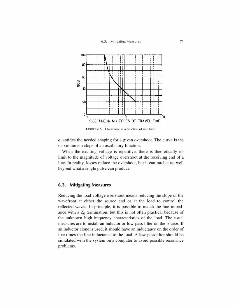
6.3. Mitigating Measures 71
quantifies the needed shaping for a given overshoot. The curve is themaximum envelope of an oscillatory function.
When the exciting voltage is repetitive, there is theoretically nolimit to the magnitude of voltage overshoot at the receiving end of aline. In reality, losses reduce the overshoot, but it can ratchet up wellbeyond what a single pulse can produce.
6.3. Mitigating Measures
Reducing the load voltage overshoot means reducing the slope of thewavefront at either the source end or at the load to control thereflected waves. In principle, it is possible to match the line imped-ance with a Z0 termination, but this is not often practical because ofthe unknown high-frequency characteristics of the load. The usualmeasures are to install an inductor or low-pass filter on the source. Ifan inductor alone is used, it should have an inductance on the order offive times the line inductance to the load. A low-pass filter should besimulated with the system on a computer to avoid possible resonanceproblems.
FIGURE 6.5 Overshoot as a function of rise time.

72 6 ◊ Traveling Waves
Installing a surge capacitor at the motor is valuable when the motorterminals are accessible to the drive designer. The capacitor will tendto reduce the end turn effects that can damage motor windings. How-ever, the capacitor may need a series damping resistor and, again, acomputer simulation is suggested.
73
Chapter 7
Transformers and Reactors
Transformers form a special class of components in power electron-ics. The design and performance of many systems are criticallydependent on the design and performance of their associated trans-formers, and the transformer often forms the major cost item in thesystem. It will often pay in performance, reliability, and economy ifthe power electronics design engineer understands transformers andhas a technical dialog with the transformer vendor. It is also a goodidea to have the current IEEE C57 series of transformer standardsavailable. These standards may be purchased from the publicationsdepartment of the IEEE in a single, bound volume.
The author once served as an expert witness in a lawsuit in which adrive manufacturer sued a transformer vendor for transformers thatfailed in a foreign steel mill. The problem was caused by radial fluxgenerating eddy currents in an electrostatic shield. The transformerhad a full axial length primary and two axially stacked secondariesthat conducted alternately. The shield overheated, the insulationfailed, and the vendor was held responsible for a faulty design. Hadthe customer explained the service conditions to the vendor ratherthan relying on a standard specification, the problem might have beenavoided.
74 7
◊
Transformers and Reactors
7.1. Transformer Basics
A review of coupled circuit equations is a good starting point for adiscussion of transformers, because it is wise to keep them in mindwhen examining transformer characteristics. First, we examine a sim-ple pair of coupled coils. Figure 7.1 shows two coils in proximity withinstantaneous voltages and currents as indicated.
The magnetic fields of these two coils have common regions, andthe coils are therefore said to be
coupled
, and a coefficient of cou-pling,
k
, defines the degree of coupling. If the coils have induc-tances
L
1
and
L
2
, then a mutual inductance can be defined such that
M
=
k
(
L
1
L
2
)
1/2
. The equations for voltages and currents can now bewritten. For the two conditions of coil 2 open circuited and short cir-cuited with coil 1 excited,
These can then be solved to yield
Loc
=
L
1
and
Lsc
=
L
1
–
M
2
/
L
2
where
Loc
and
Lsc
are the open circuit and short circuit inductances,respectively. Then,
FIGURE 7.1 Coupled coils.
o.c. e1 L1
di1dt-------= s.c. e1 L1
di1dt------- M
di2dt-------–=
0 Mdi1dt------- L2
di2dt-------+–=
k 1LscLoc---------⎝ ⎠
⎛ ⎞– 1XscXoc----------⎝ ⎠
⎛ ⎞–= =
7.1. Transformer Basics 75
Figure 7.2 shows an equivalent circuit for an idealized transformer withno losses. From the equations for Fig. 7.1,
Loc
=
L
1
,
Lsc
=
L
1
–
M
2
/
L
2
,
A
=
L
1
–
M,
and
B
=
L
2
–
M
.
A
and
B
are defined as the primary andsecondary leakage inductances, respectively, and
M
is the magnetiz-ing inductance. More usually, the inductances are replaced by theirreactances at the operating frequency. If the turns ratio is
n
:1, primaryand secondary quantities are related by
Es
=
Ep/n
and
Is
=
Ip
×
n
.These quantities are often expressed in percentage or per unit quan-
tities, since they can then be used to compare transformers across allratings, designs, and leakages. The leakage reactance in percent isequal to the full-load voltage drop as a percent of rated voltage forthat winding. Note that this is a vector voltage drop, and the effect ofthis drop on the terminal voltage will depend on the current phaseangle. The exciting current is expressed as a fraction or percent ofrated load current which, in turn, is rated voltage divided by the mag-netizing reactance.
Considering a typical transformer with a total leakage reactance of6% and an exciting current of 5%, equal to a magnetizing reactance of100/0.05 or 2000%,
Thus, the typical iron-core transformer has a very high coefficient ofcoupling. Air-core coils, on the other hand, generally have much
FIGURE 7.2 Ideal transformer.
k 16
2000------------⎝ ⎠
⎛ ⎞–1 2⁄
0.9985= =
76 7
◊
Transformers and Reactors
lower coupling coefficients, and they must be wound bifilar or coaxialto achieve a high coupling factor. Some transformers designed forconstant current output are built with an air gap that provides interme-diate coupling coefficients.
In the real world, the ideal transformer is complicated by excitingcurrent and leakage losses as shown in Fig. 7.3. Except for some veryspecial types, nearly all transformers are made with laminated ironcores to maximize the coupling between the coils. Exciting current isthe current required to produce the desired flux density in the iron plusthe current due to hysteresis and eddy current losses in the iron. A typ-ical exciting current will be in the range of 3 to 8% of rated primaryload current, and total leakage reactances will produce a 3 to 10%voltage drop at full load. Again, this is a vector drop and will notdirectly subtract from secondary voltage except for the case of anearly zero power factor lagging load. The exciting current and lossresistances are usually neglected in transformer regulation equations.Total losses vary widely but may be approximated as 0.25 to 1.0% ofrated load for transformers from 1000 to 10,000 kVA. Larger trans-formers tend to have lower losses and smaller transformers higherlosses than those indicated.
Primary and secondary leakage reactances can be transferred fromone winding to the other by the equations
XTp
=
Xp
+
n
2
Xs
and
XTs
=
Xs
+
Xp/n
2
where
XTp
and
XTs
are the total leakage reactancesin ohms, referred to the primary and secondary, respectively, with
n
the number of turns. When a transformer impedance is simply speci-
FIGURE 7.3 Typical transformer representation.
7.1. Transformer Basics 77
fied as
Z
%, one may assume the impedance is reactive, and the sec-ondary voltage drop at rated current will be
Z
% or
Zpu
of ratedvoltage. If the transformer is faulted, the rms symmetrical fault cur-rent will be 1/Zpu times rated current. For example, a transformerwith 5% reactance, 0.05 pu, will have a symmetrical short circuit cur-rent of 20 times rated current, 20 pu. These numbers assume thesource impedance is negligible.
Percent regulation in a transformer is defined as 100(VNL – VFL)/VFLwhere VNL and VFL are the no-load and full-load voltages, respec-tively. Regulation can be determined from the phasor diagram shownin Fig. 7.4.
Power transformers intended for converters often are made with twosecondaries, one delta connected and the other wye connected. Thetwo secondary voltages are then 30° out of phase, and it is possible togreatly reduce some of the harmonic currents in the primary thatresult from the nonlinear secondary loading. The diagram is shown inFig. 7.5.
The characteristics of this transformer can be determined on test. Astypically used, the per unit reactances of S1 and S2 are equal. If thethree windings are individually shorted one at a time with the otherwindings energized, the following equations result:
FIGURE 7.4 Transformer regulation phasor diagram.
78 7 ◊ Transformers and Reactors
if P to S1 = X, P to S2 = X, S1 to S2 = Y
then, A + B = X, A + C = X, B + C = Y
and A = X – Y/2, B = Y/2, C = Y/2
If the secondaries are tightly coupled, then Y is very low, and theequivalent reactance is nearly all in the primary. If they are poorlycoupled so that Y is high, the primary reactance, A, may go negative.If the secondaries have a particular coupling to each other, the primaryreactance can be zero, and all the equivalent reactance is in the sec-ondaries. A negative primary reactance implies a regulation character-istic in which the secondary voltage of a converter falls less underload, and this can be used to advantage to improve regulation. At theother end of the spectrum, loose coupling from the primary to the twosecondaries can be used to reduce the short circuit current.
7.2. Construction
Two basic core and coil arrangements, shell form and core form, areused in transformers. Both are illustrated in Fig. 7.6 in single-phaseversions. The shell form is appropriate for the largest and highest-voltage transformers. The windings are pancake coils that arestacked prior to assembly of the core. The coils are surrounded bycore material except for the end turns, and they can be braced for
FIGURE 7.5 Three-winding transformer.
7.1. Construction 79
high fault currents and interleaved for low leakage reactance. Shellform transformers are almost invariably oil filled, and units as largeas 500 MVA have been built for generator transformers.
The core form design places the coils over a vertical leg of lamina-tions. The coils, in effect, surround the core. Coils are lathe woundwith either circular or rectangular cross sections. This construction isappropriate for smaller transformers and to dry-type units. Core formconstruction in the 10 kVA to 20 MVA range is quite common. Onefact that makes core form designs difficult in very large units is brac-ing for fault currents. Since force is proportional to the square of thecurrent, a fault current of 20 times normal creates 400 times normalstresses. The coils are subject to large radial forces, and they have nobracing except for the circumferential coil wrapper. The inner wind-ing tends to be compressed against the core on faults, while the outerwinding heads for outer space. The core, or at least the core corners,may be covered with polyester fiberglass to protect the inner wind-ing, and the outer winding may have a fiberglass wrap. There is alsoan axial force that must be retained by blocking the coil ends againstthe core. Nonetheless, the vast majority of medium-voltage andmedium-power transformers are core form because of manufacturingeconomies.
Two variants on the core form transformer are worthy of mention.The coils may be cast in resin, often an epoxy, for environmental pro-tection. If air cooling is used, a radial gap may be provided between
FIGURE 7.6 Transformer cross sections.
80 7 ◊ Transformers and Reactors
primary and secondary as a cooling duct. These transformers are usu-ally relatively large for their ratings. Another technique relies on castcoils made with hollow conductors that are liquid cooled. Such directliquid cooling has been extended to 15-kV class primaries in recentyears, with deionized coolant used to control electrolysis. A propyleneglycol and water mix is used for protection from freezing. Althoughthe liquid-cooled transformers require demineralizer tanks, pumps,and heat exchangers, such items are often used with the higher-powersemiconductors for direct cooling. The transformer, semiconductors,and bus work may share a common liquid cooling system. Sucharrangements are especially suited to applications in which good qual-ity cooling air may not be available. Examples are foundries, glassplants, metal mills, and the like where expensive filters and ductworkcan be eliminated. Heat exchangers are either water-to-air or water-to-water and may be part of a larger plant system. One note of cautionshould be sounded on water cooling. If a glycol mix is used, the gly-col must be chemical grade. Commercial antifreeze fluids have rustinhibitors and other additives that will increase the conductivity.
The general characteristics of oil-filled and dry-type transformersare summarized in Table 7.1. Oil-filled transformers employ mineraloil both as an insulation system and as a heat exchange medium. Thetypical insulation is pressboard or kraft paper, both of which are sat-urated by oil. The dielectric constants of these materials closelymatch the dielectric constant of the oil so that no electric field dis-continuities are caused by the insulation. Hot oil is introduced intothe heated windings under vacuum so that all entrained air is elimi-nated from both the oil and insulation. Heating the oil reduces itsviscosity and facilitates penetration. The insulation is totally soakedby the oil, and the oil is relied on to eliminate air voids that woulddeteriorate the insulation from corona discharge. Furthermore, thedielectric properties of the oil mean that the internal spacingsbetween components at different voltages can be much less than thespacings required in air. The operating temperature of the oil is lim-ited by the gradual loss of its insulating qualities through the forma-
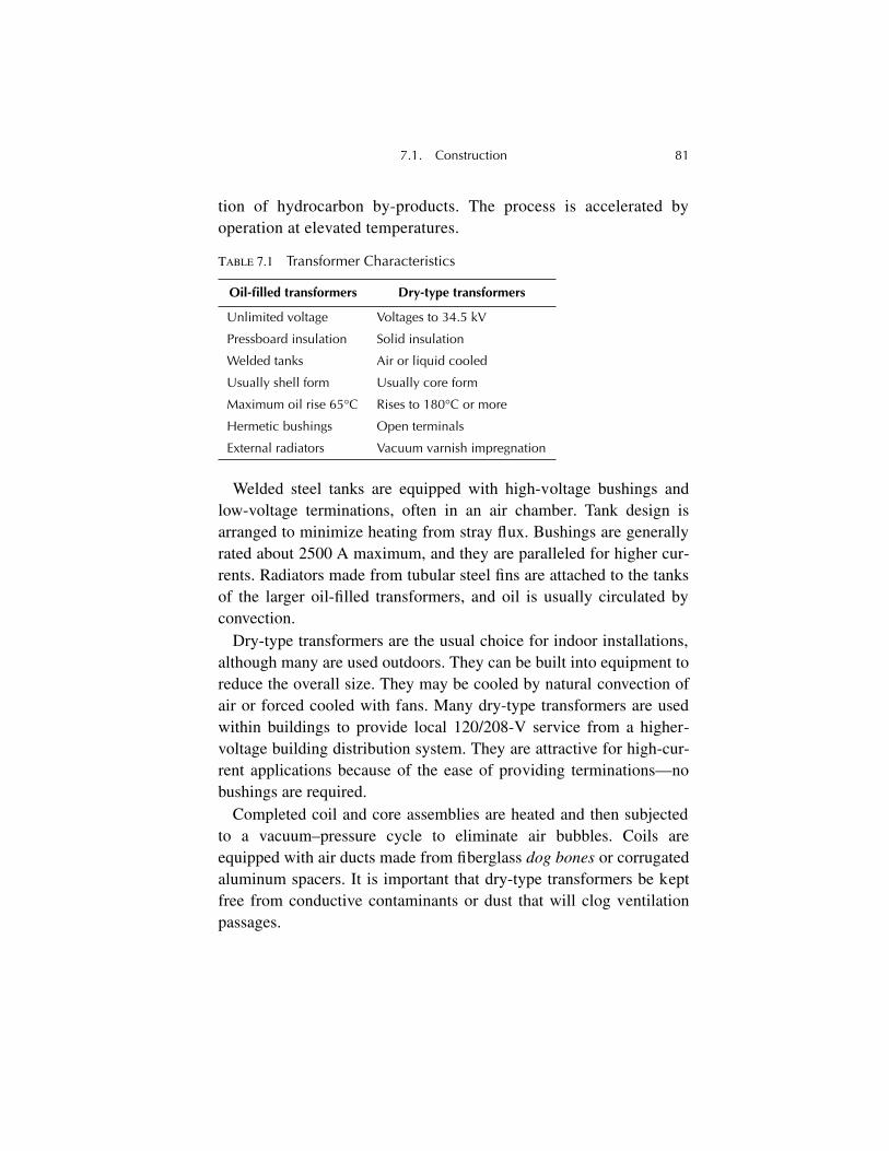
7.1. Construction 81
tion of hydrocarbon by-products. The process is accelerated byoperation at elevated temperatures.
Welded steel tanks are equipped with high-voltage bushings andlow-voltage terminations, often in an air chamber. Tank design isarranged to minimize heating from stray flux. Bushings are generallyrated about 2500 A maximum, and they are paralleled for higher cur-rents. Radiators made from tubular steel fins are attached to the tanksof the larger oil-filled transformers, and oil is usually circulated byconvection.
Dry-type transformers are the usual choice for indoor installations,although many are used outdoors. They can be built into equipment toreduce the overall size. They may be cooled by natural convection ofair or forced cooled with fans. Many dry-type transformers are usedwithin buildings to provide local 120/208-V service from a higher-voltage building distribution system. They are attractive for high-cur-rent applications because of the ease of providing terminations—nobushings are required.
Completed coil and core assemblies are heated and then subjectedto a vacuum–pressure cycle to eliminate air bubbles. Coils areequipped with air ducts made from fiberglass dog bones or corrugatedaluminum spacers. It is important that dry-type transformers be keptfree from conductive contaminants or dust that will clog ventilationpassages.
TABLE 7.1 Transformer Characteristics
Oil-filled transformers Dry-type transformers
Unlimited voltage Voltages to 34.5 kV
Pressboard insulation Solid insulation
Welded tanks Air or liquid cooled
Usually shell form Usually core form
Maximum oil rise 65°C Rises to 180°C or more
Hermetic bushings Open terminals
External radiators Vacuum varnish impregnation
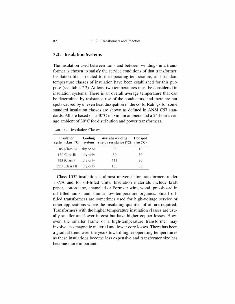
82 7 ◊ Transformers and Reactors
7.3. Insulation Systems
The insulation used between turns and between windings in a trans-former is chosen to satisfy the service conditions of that transformer.Insulation life is related to the operating temperature, and standardtemperature classes of insulation have been established for this pur-pose (see Table 7.2). At least two temperatures must be considered ininsulation systems. There is an overall average temperature that canbe determined by resistance rise of the conductors, and there are hotspots caused by uneven heat dissipation in the coils. Ratings for somestandard insulation classes are shown as defined in ANSI C57 stan-dards. All are based on a 40°C maximum ambient and a 24-hour aver-age ambient of 30°C for distribution and power transformers.
Class 105° insulation is almost universal for transformers under1 kVA and for oil-filled units. Insulation materials include kraftpaper, cotton tape, enameled or Formvar wire, wood, pressboard inoil filled units, and similar low-temperature organics. Small oil-filled transformers are sometimes used for high-voltage service orother applications where the insulating qualities of oil are required.Transformers with the higher temperature insulation classes are usu-ally smaller and lower in cost but have higher copper losses. How-ever, the smaller frame of a high-temperature transformer mayinvolve less magnetic material and lower core losses. There has beena gradual trend over the years toward higher operating temperaturesas these insulations become less expensive and transformer size hasbecome more important.
TABLE 7.2 Insulation Classes
Insulation system class (°C)
Cooling system
Average winding rise by resistance (°C)
Hot spot rise (°C)
105 (Class A) dry or oil 55 10
150 Class B) dry only 80 30
185 (Class F) dry only 115 30
220 (Class H) dry only 150 30
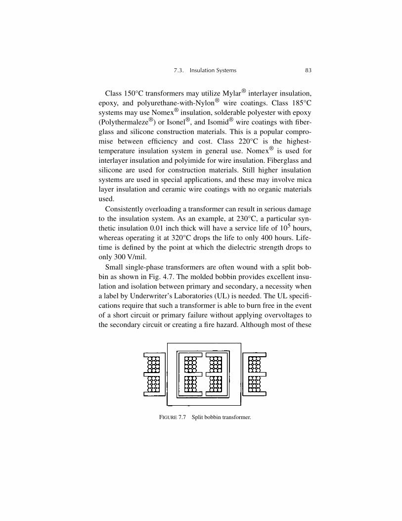
7.3. Insulation Systems 83
Class 150°C transformers may utilize Mylar® interlayer insulation,epoxy, and polyurethane-with-Nylon® wire coatings. Class 185°Csystems may use Nomex® insulation, solderable polyester with epoxy(Polythermaleze®) or Isonel®, and Isomid® wire coatings with fiber-glass and silicone construction materials. This is a popular compro-mise between efficiency and cost. Class 220°C is the highest-temperature insulation system in general use. Nomex® is used forinterlayer insulation and polyimide for wire insulation. Fiberglass andsilicone are used for construction materials. Still higher insulationsystems are used in special applications, and these may involve micalayer insulation and ceramic wire coatings with no organic materialsused.
Consistently overloading a transformer can result in serious damageto the insulation system. As an example, at 230°C, a particular syn-thetic insulation 0.01 inch thick will have a service life of 105 hours,whereas operating it at 320°C drops the life to only 400 hours. Life-time is defined by the point at which the dielectric strength drops toonly 300 V/mil.
Small single-phase transformers are often wound with a split bob-bin as shown in Fig. 4.7. The molded bobbin provides excellent insu-lation and isolation between primary and secondary, a necessity whena label by Underwriter’s Laboratories (UL) is needed. The UL specifi-cations require that such a transformer is able to burn free in the eventof a short circuit or primary failure without applying overvoltages tothe secondary circuit or creating a fire hazard. Although most of these
FIGURE 7.7 Split bobbin transformer.
84 7 ◊ Transformers and Reactors
transformers are rated for Class 105°C operation, the insulation isoften Class 220°C so that isolation is maintained even when the pri-mary or secondary burns. Many small transformers intended forprinted circuit mounting are made this way.
As mentioned earlier, transformer insulation is treated to remove allbubbles and air pockets. The air has a lower dielectric constant thanthe insulation materials, so an air bubble will have a higher voltagegradient than the surrounding insulation. This gradient may be highenough to ionize the air and begin a corona discharge within the bub-ble. One result of this corona is the formation of ozone, a powerfuloxidizing agent that can damage the adjacent insulation and result inultimate failure. The same thing can happen from operating the insu-lation itself at too high a voltage stress. Two 6900-V, 3000-kVA dry-type transformers installed in a steel mill some years ago failed afteronly a month in service. The designer had used too little interlayerinsulation, and corona destroyed it while it was still under warranty.The transformers had to be returned to the vendor for a rewind at hisexpense.
7.4. Basic Insulation Level
The AC operating voltage of a transformer winding is shared equallyby all the turns in the winding, and the turn-to-turn voltages are con-stant. Surge voltages, however, can create much higher turn-to-turnvoltages at the exposed end of the winding due to capacitance distri-butions. Figure 7.8 shows an elementary five-section representationof these capacitances. The turn-to-turn and turn-to-ground capaci-tances are equal, and the inductance is large enough to be ignored.Note that nearly 62% of the incident surge voltage is taken up on thefirst turns. The turn-to-turn spacing and turn-to-turn insulation aresometimes increased at the HV end of windings in medium-voltagetransformers, and grading shields are used to improve the surge volt-age distributions.
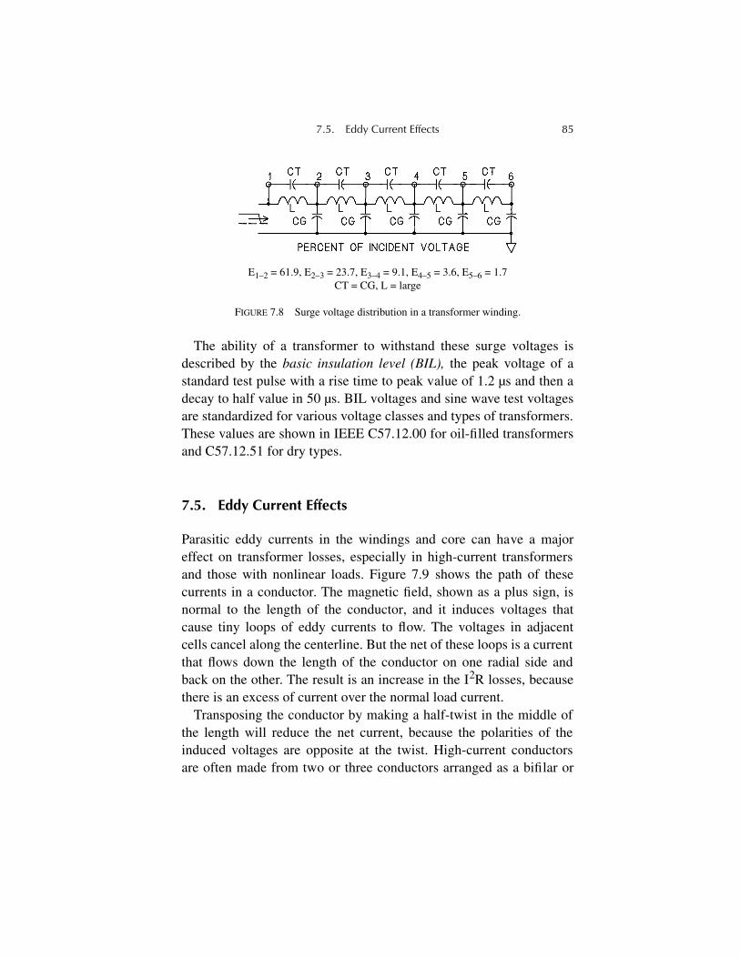
7.5. Eddy Current Effects 85
The ability of a transformer to withstand these surge voltages isdescribed by the basic insulation level (BIL), the peak voltage of astandard test pulse with a rise time to peak value of 1.2 µs and then adecay to half value in 50 µs. BIL voltages and sine wave test voltagesare standardized for various voltage classes and types of transformers.These values are shown in IEEE C57.12.00 for oil-filled transformersand C57.12.51 for dry types.
7.5. Eddy Current Effects
Parasitic eddy currents in the windings and core can have a majoreffect on transformer losses, especially in high-current transformersand those with nonlinear loads. Figure 7.9 shows the path of thesecurrents in a conductor. The magnetic field, shown as a plus sign, isnormal to the length of the conductor, and it induces voltages thatcause tiny loops of eddy currents to flow. The voltages in adjacentcells cancel along the centerline. But the net of these loops is a currentthat flows down the length of the conductor on one radial side andback on the other. The result is an increase in the I2R losses, becausethere is an excess of current over the normal load current.
Transposing the conductor by making a half-twist in the middle ofthe length will reduce the net current, because the polarities of theinduced voltages are opposite at the twist. High-current conductorsare often made from two or three conductors arranged as a bifilar or
FIGURE 7.8 Surge voltage distribution in a transformer winding.
E1–2 = 61.9, E2–3 = 23.7, E3–4 = 9.1, E4–5 = 3.6, E5–6 = 1.7CT = CG, L = large
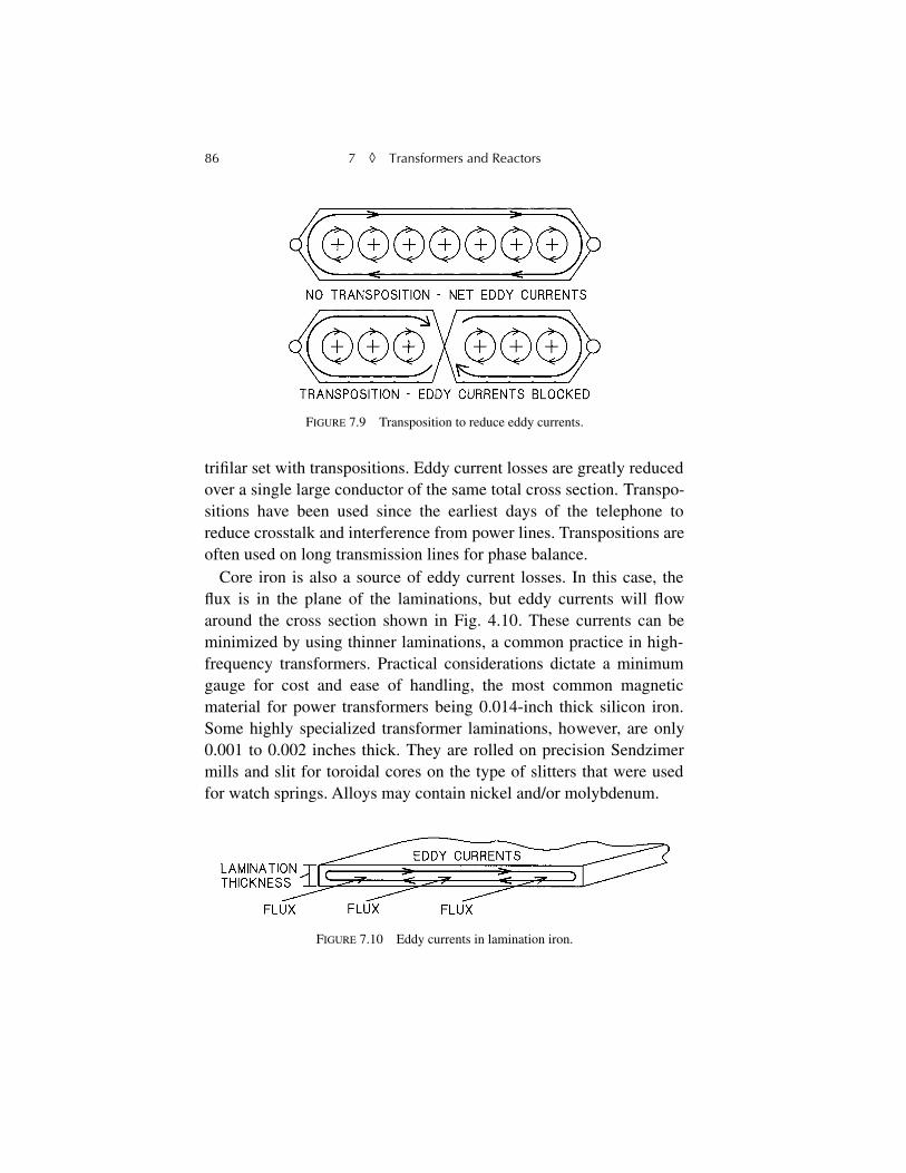
86 7 ◊ Transformers and Reactors
trifilar set with transpositions. Eddy current losses are greatly reducedover a single large conductor of the same total cross section. Transpo-sitions have been used since the earliest days of the telephone toreduce crosstalk and interference from power lines. Transpositions areoften used on long transmission lines for phase balance.
Core iron is also a source of eddy current losses. In this case, theflux is in the plane of the laminations, but eddy currents will flowaround the cross section shown in Fig. 4.10. These currents can beminimized by using thinner laminations, a common practice in high-frequency transformers. Practical considerations dictate a minimumgauge for cost and ease of handling, the most common magneticmaterial for power transformers being 0.014-inch thick silicon iron.Some highly specialized transformer laminations, however, are only0.001 to 0.002 inches thick. They are rolled on precision Sendzimermills and slit for toroidal cores on the type of slitters that were usedfor watch springs. Alloys may contain nickel and/or molybdenum.
FIGURE 7.9 Transposition to reduce eddy currents.
FIGURE 7.10 Eddy currents in lamination iron.
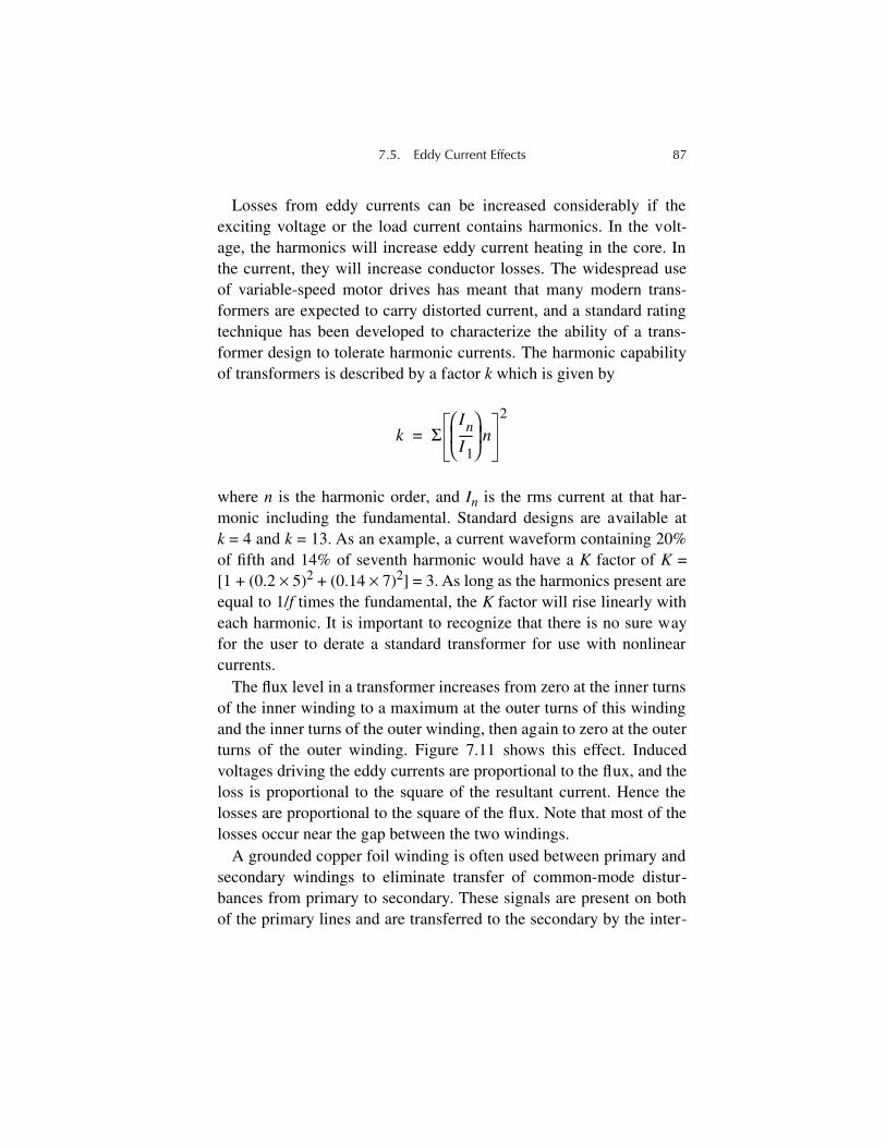
7.5. Eddy Current Effects 87
Losses from eddy currents can be increased considerably if theexciting voltage or the load current contains harmonics. In the volt-age, the harmonics will increase eddy current heating in the core. Inthe current, they will increase conductor losses. The widespread useof variable-speed motor drives has meant that many modern trans-formers are expected to carry distorted current, and a standard ratingtechnique has been developed to characterize the ability of a trans-former design to tolerate harmonic currents. The harmonic capabilityof transformers is described by a factor k which is given by
where n is the harmonic order, and In is the rms current at that har-monic including the fundamental. Standard designs are available atk = 4 and k = 13. As an example, a current waveform containing 20%of fifth and 14% of seventh harmonic would have a K factor of K =[1 + (0.2 × 5)2 + (0.14 × 7)2] = 3. As long as the harmonics present areequal to 1/f times the fundamental, the K factor will rise linearly witheach harmonic. It is important to recognize that there is no sure wayfor the user to derate a standard transformer for use with nonlinearcurrents.
The flux level in a transformer increases from zero at the inner turnsof the inner winding to a maximum at the outer turns of this windingand the inner turns of the outer winding, then again to zero at the outerturns of the outer winding. Figure 7.11 shows this effect. Inducedvoltages driving the eddy currents are proportional to the flux, and theloss is proportional to the square of the resultant current. Hence thelosses are proportional to the square of the flux. Note that most of thelosses occur near the gap between the two windings.
A grounded copper foil winding is often used between primary andsecondary windings to eliminate transfer of common-mode distur-bances from primary to secondary. These signals are present on bothof the primary lines and are transferred to the secondary by the inter-
k ΣIn
I1-----
⎝ ⎠⎜ ⎟⎛ ⎞
n2
=
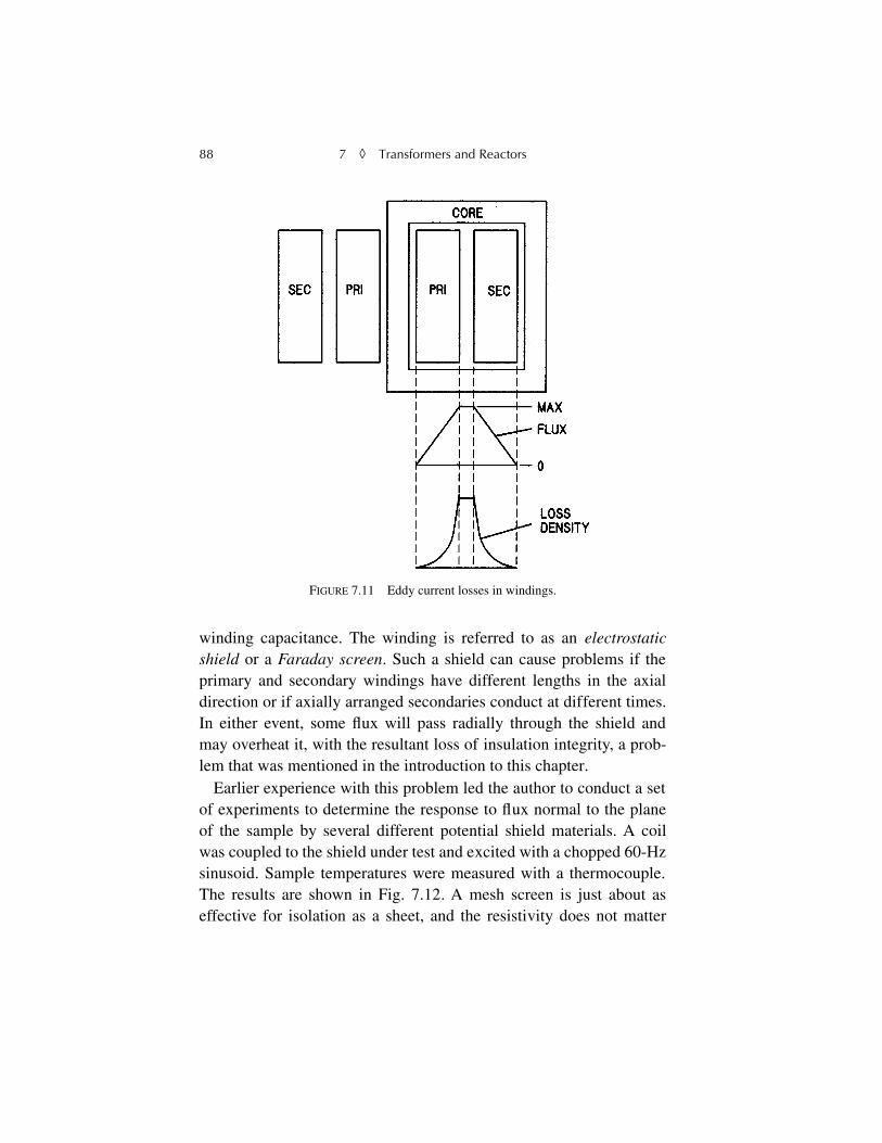
88 7 ◊ Transformers and Reactors
winding capacitance. The winding is referred to as an electrostaticshield or a Faraday screen. Such a shield can cause problems if theprimary and secondary windings have different lengths in the axialdirection or if axially arranged secondaries conduct at different times.In either event, some flux will pass radially through the shield andmay overheat it, with the resultant loss of insulation integrity, a prob-lem that was mentioned in the introduction to this chapter.
Earlier experience with this problem led the author to conduct a setof experiments to determine the response to flux normal to the planeof the sample by several different potential shield materials. A coilwas coupled to the shield under test and excited with a chopped 60-Hzsinusoid. Sample temperatures were measured with a thermocouple.The results are shown in Fig. 7.12. A mesh screen is just about aseffective for isolation as a sheet, and the resistivity does not matter
FIGURE 7.11 Eddy current losses in windings.
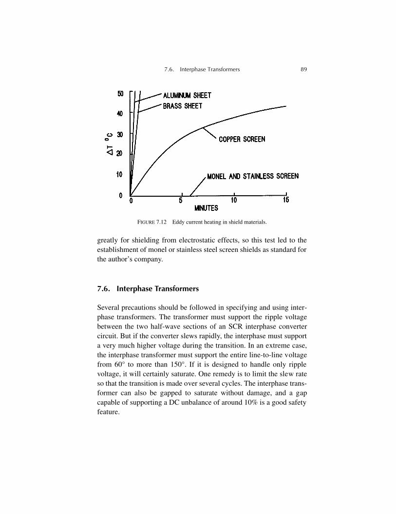
7.6. Interphase Transformers 89
greatly for shielding from electrostatic effects, so this test led to theestablishment of monel or stainless steel screen shields as standard forthe author’s company.
7.6. Interphase Transformers
Several precautions should be followed in specifying and using inter-phase transformers. The transformer must support the ripple voltagebetween the two half-wave sections of an SCR interphase convertercircuit. But if the converter slews rapidly, the interphase must supporta very much higher voltage during the transition. In an extreme case,the interphase transformer must support the entire line-to-line voltagefrom 60° to more than 150°. If it is designed to handle only ripplevoltage, it will certainly saturate. One remedy is to limit the slew rateso that the transition is made over several cycles. The interphase trans-former can also be gapped to saturate without damage, and a gapcapable of supporting a DC unbalance of around 10% is a good safetyfeature.
FIGURE 7.12 Eddy current heating in shield materials.
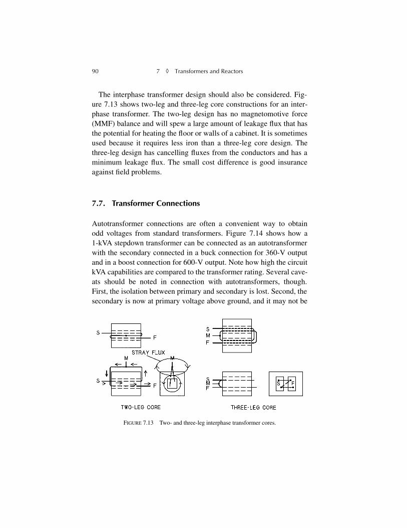
90 7 ◊ Transformers and Reactors
The interphase transformer design should also be considered. Fig-ure 7.13 shows two-leg and three-leg core constructions for an inter-phase transformer. The two-leg design has no magnetomotive force(MMF) balance and will spew a large amount of leakage flux that hasthe potential for heating the floor or walls of a cabinet. It is sometimesused because it requires less iron than a three-leg core design. Thethree-leg design has cancelling fluxes from the conductors and has aminimum leakage flux. The small cost difference is good insuranceagainst field problems.
7.7. Transformer Connections
Autotransformer connections are often a convenient way to obtainodd voltages from standard transformers. Figure 7.14 shows how a1-kVA stepdown transformer can be connected as an autotransformerwith the secondary connected in a buck connection for 360-V outputand in a boost connection for 600-V output. Note how high the circuitkVA capabilities are compared to the transformer rating. Several cave-ats should be noted in connection with autotransformers, though.First, the isolation between primary and secondary is lost. Second, thesecondary is now at primary voltage above ground, and it may not be
FIGURE 7.13 Two- and three-leg interphase transformer cores.
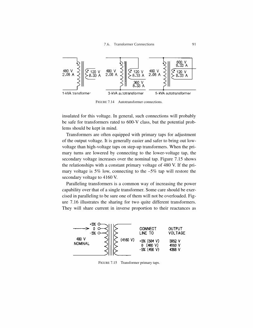
7.6. Transformer Connections 91
insulated for this voltage. In general, such connections will probablybe safe for transformers rated to 600-V class, but the potential prob-lems should be kept in mind.
Transformers are often equipped with primary taps for adjustmentof the output voltage. It is generally easier and safer to bring out low-voltage than high-voltage taps on step-up transformers. When the pri-mary turns are lowered by connecting to the lower-voltage tap, thesecondary voltage increases over the nominal tap. Figure 7.15 showsthe relationships with a constant primary voltage of 480 V. If the pri-mary voltage is 5% low, connecting to the –5% tap will restore thesecondary voltage to 4160 V.
Paralleling transformers is a common way of increasing the powercapability over that of a single transformer. Some care should be exer-cised in paralleling to be sure one of them will not be overloaded. Fig-ure 7.16 illustrates the sharing for two quite different transformers.They will share current in inverse proportion to their reactances as
FIGURE 7.14 Autotransformer connections.
FIGURE 7.15 Transformer primary taps.
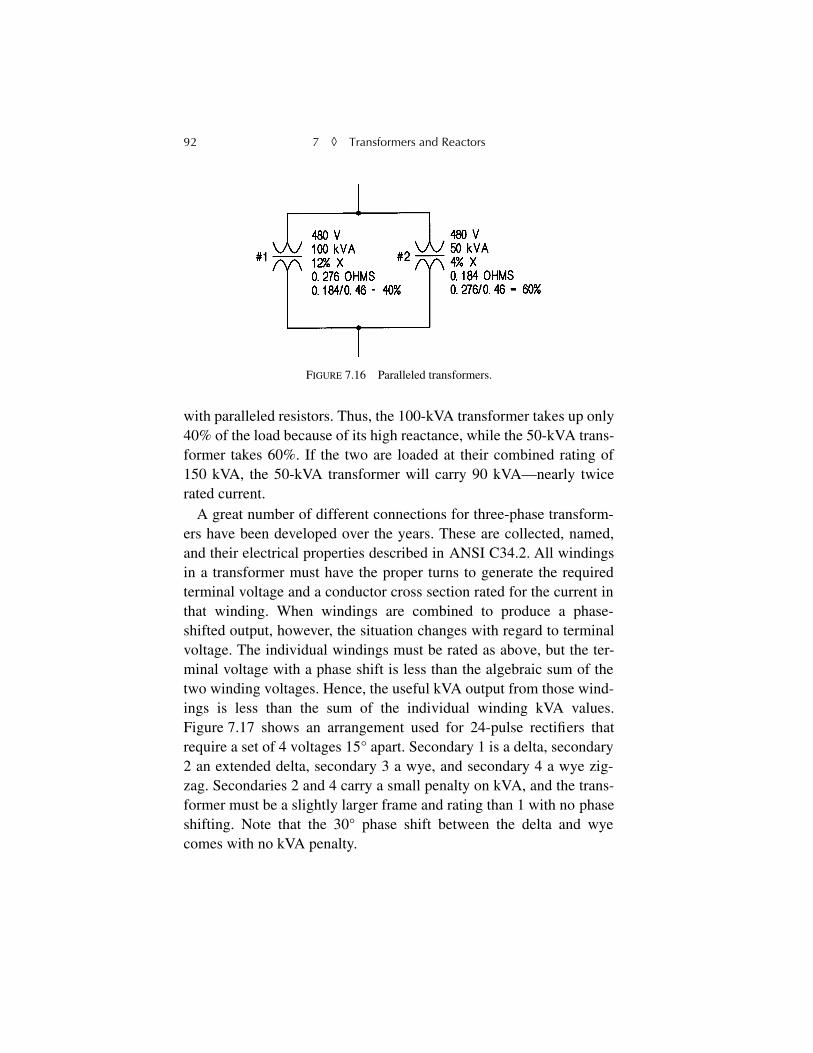
92 7 ◊ Transformers and Reactors
with paralleled resistors. Thus, the 100-kVA transformer takes up only40% of the load because of its high reactance, while the 50-kVA trans-former takes 60%. If the two are loaded at their combined rating of150 kVA, the 50-kVA transformer will carry 90 kVA—nearly twicerated current.
A great number of different connections for three-phase transform-ers have been developed over the years. These are collected, named,and their electrical properties described in ANSI C34.2. All windingsin a transformer must have the proper turns to generate the requiredterminal voltage and a conductor cross section rated for the current inthat winding. When windings are combined to produce a phase-shifted output, however, the situation changes with regard to terminalvoltage. The individual windings must be rated as above, but the ter-minal voltage with a phase shift is less than the algebraic sum of thetwo winding voltages. Hence, the useful kVA output from those wind-ings is less than the sum of the individual winding kVA values.Figure 7.17 shows an arrangement used for 24-pulse rectifiers thatrequire a set of 4 voltages 15° apart. Secondary 1 is a delta, secondary2 an extended delta, secondary 3 a wye, and secondary 4 a wye zig-zag. Secondaries 2 and 4 carry a small penalty on kVA, and the trans-former must be a slightly larger frame and rating than 1 with no phaseshifting. Note that the 30° phase shift between the delta and wyecomes with no kVA penalty.
FIGURE 7.16 Paralleled transformers.
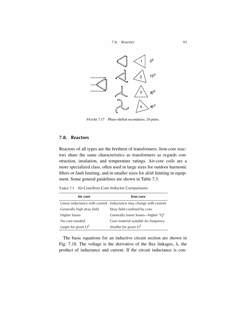
7.8. Reactors 93
7.8. Reactors
Reactors of all types are the brethren of transformers. Iron-core reac-tors share the same characteristics as transformers as regards con-struction, insulation, and temperature ratings. Air-core coils are amore specialized class, often used in large sizes for outdoor harmonicfilters or fault limiting, and in smaller sizes for di/dt limiting in equip-ment. Some general guidelines are shown in Table 7.3.
The basic equations for an inductive circuit section are shown inFig. 7.18. The voltage is the derivative of the flux linkages, λ, theproduct of inductance and current. If the circuit inductance is con-
TABLE 7.3 Air-Core/Iron-Core Inductor Comparisons
Air core Iron core
Linear inductance with current Inductance may change with current
Generally high stray field Stray field confined by core
Higher losses Generally lower losses—higher “Q”
No core needed Core material suitable for frequency
Larger for given LI2 Smaller for given LI2
FIGURE 7.17 Phase-shifted secondaries, 24-pulse.
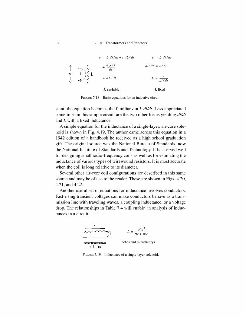
94 7 ◊ Transformers and Reactors
stant, the equation becomes the familiar e = L di/dt. Less appreciatedsometimes in this simple circuit are the two other forms yielding di/dtand L with a fixed inductance.
A simple equation for the inductance of a single-layer, air-core sole-noid is shown in Fig. 4.19. The author came across this equation in a1942 edition of a handbook he received as a high school graduationgift. The original source was the National Bureau of Standards, nowthe National Institute of Standards and Technology. It has served wellfor designing small radio-frequency coils as well as for estimating theinductance of various types of wirewound resistors. It is most accuratewhen the coil is long relative to its diameter.
Several other air-core coil configurations are described in this samesource and may be of use to the reader. These are shown in Figs. 4.20,4.21, and 4.22.
Another useful set of equations for inductance involves conductors.Fast-rising transient voltages can make conductors behave as a trans-mission line with traveling waves, a coupling inductance, or a voltagedrop. The relationships in Table 7.4 will enable an analysis of induc-tances in a circuit.
FIGURE 7.18 Basic equations for an inductive circuit.
e L di dt⁄ i dL dt⁄+=
d Li( )dt
-------------=
dλ dt⁄=
e L di dt⁄=
di dt⁄ e L⁄=
Le
di dt⁄--------------=
L variable L fixed
FIGURE 7.19 Inductance of a single-layer solenoid.
Lr
2n
2
9r 10k+---------------------=
inches and microhenrys
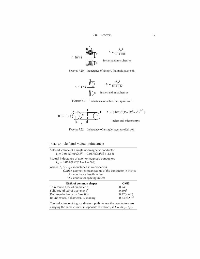
7.8. Reactors 95
TABLE 7.4 Self and Mutual Inductances
Self-inductance of a single nonmagnetic conductorLs = 0.061f(ln(f/GMR) + 0.017(GMR/f) + 2.18)
Mutual inductance of two nonmagnetic conductorsLm = 0.061f(ln(2f/D) – 1 + D/f))
where Ls or Lm = inductance in microhenrysGMR = geometric mean radius of the conductor in inches
f = conductor length in feetD = conductor spacing in feet
GMR of common shapesThin round tube of diameter dSolid round bar of diameter dRectangular bar, a by b sectionRound wires, d diameter, D spacing
GMR0.5d0.39d0.22(a + b)0.63(dD)1/2
The inductance of a go-and-return path, where the conductors are carrying the same current in opposite directions, is L = 2(Ls – Lm).
FIGURE 7.20 Inductance of a short, fat, multilayer coil.
Lr
2n
2
9r 10k+---------------------=
inches and microhenrys
FIGURE 7.21 Inductance of a thin, flat, spiral coil.
Lr
2n
2
8r 11c+---------------------=
inches and microhenrys
FIGURE 7.22 Inductance of a single-layer toroidal coil.
L 0.032n2
R R2
r2
–( )1 2⁄
–[ ]=
inches and microhenrys
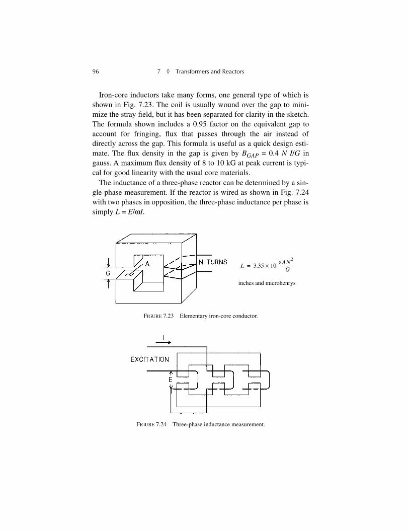
96 7 ◊ Transformers and Reactors
Iron-core inductors take many forms, one general type of which isshown in Fig. 7.23. The coil is usually wound over the gap to mini-mize the stray field, but it has been separated for clarity in the sketch.The formula shown includes a 0.95 factor on the equivalent gap toaccount for fringing, flux that passes through the air instead ofdirectly across the gap. This formula is useful as a quick design esti-mate. The flux density in the gap is given by BGAP = 0.4 N I/G ingauss. A maximum flux density of 8 to 10 kG at peak current is typi-cal for good linearity with the usual core materials.
The inductance of a three-phase reactor can be determined by a sin-gle-phase measurement. If the reactor is wired as shown in Fig. 7.24with two phases in opposition, the three-phase inductance per phase issimply L = E/ωI.
FIGURE 7.23 Elementary iron-core conductor.
L 3.35 108– AN
2
G-----------×=
inches and microhenrys
FIGURE 7.24 Three-phase inductance measurement.
7.9. Units 97
7.9. Units
Sooner or later, in any text on magnetics, the subject of units of mea-surement must be considered. The author regrets having to introducethe matter, because three different systems of units are in general use.Physicists may prefer CGS units, engineers in general use MKS units,and transformer designers use English units. The international stan-dard (SI) is the MKS system, and usage trends toward this system.Table 7.5 summarizes the present situation in magnetics units, andthis table may serve either as a handy reference for the reader or apage to be torn out to line the bird cage.
7.10. Cooling
Oil filled transformers can generally take care of themselves, sincethey are seldom built into other enclosures. Dry types, however, areoften purchased as core and coils with no enclosure and built intoequipment. The burden then falls on the equipment designer to provideadequate cooling for the transformer. When the transformer is pur-chased with integral fans, these are usually located at the bottom of theassembly, and they direct cooling air up through the coils. The onlyfurther requirement is to provide sufficient makeup air for cooling.
TABLE 7.5 Magnetic Units
MKS (SI) Units CGS Units English Units
Flux density B = µrµoH B = µrH B = µrµoH
Flux ϕ = AB ϕ = AB ϕ = AB
Faraday’s Law v = Ndϕ/dt v = 10–8Ndϕ/dt v = 10–8Ndϕ/dt
µo 4π × 10–7 1.0 3.192
Units A in m2 A in cm2 A in in2
B in teslas B in gauss B in lines/in2
H in amp turns/m H in oersteds H in amp turns/in
ϕ in webers ϕ in maxwells ϕ in lines
F in amp turns F in gilberts F in amp turns
98 7 ◊ Transformers and Reactors
Transformers that rely on forced air from an external source or areconvection cooled may require some attention to airflow. If no air isadmitted to the enclosure, the internal air will become heated as itrises through the coils and will tend to stratify with the hot air accu-mulating at the top of the compartment. The only heat exchange isthen by radiation and convection from the enclosure, so the obviousthing to do is to admit air at the bottom of the enclosure and exhaust itat the top. But this may not end the matter. The coils represent a highhead loss to airflow, whereas the surrounding space offers little. Cool-ing air that enters the bottom vent may simply flow directly up to thetop vent, bypassing the coils in the process. Figure 4.25 illustrates thesolution of adding a horizontal skirt to force the cooling air upthrough the coils. The skirt can be made of lightweight insulatingmaterial such as polyester fiberglass sheet.
7.11. Instrument Transformers
AC voltages and currents that are too high for direct connection tometers or protective relays can be measured with the aid of voltage
FIGURE 7.25 Skirting to improve transformer cooling.
7.10. Instrument Transformers 99
(potential) and current transformers. Voltage transformers are trans-formers with low exciting current and leakage reactance that are insu-lated for high voltage on the primary. The usual secondary voltage is120 V. These transformers are made with both single-insulator prima-ries for measuring line-to-ground voltages and double-insulator pri-maries for line-to-line metering. The transformer frame should besolidly earth grounded for safety on either type. Single-insulatortransformers can be fused with only one fuse on the high-voltage side,but double-insulator transformers must be fused on both primary con-nections to protect against a ground fault in the primary winding.Medium-voltage fuses, specially rated for voltage transformers, areavailable. Since the primary fuses must be large enough to withstandinrush currents, they only serve as short-circuit protection. The trans-former should be thermally protected by a secondary fuse and haveone side of the secondary earth grounded for safety.
Current transformers are available in both wound primary and bush-ing types. The wound primaries are like an ordinary transformer witha few primary turns and a large number of secondary turns so that alarge primary current is transformed into a small secondary current,the secondary being short circuited by the connected ammeter orrelay. This type is used mostly for low currents or high-accuracyapplications.
Bushing transformers are toroidal cores with a wound secondary,the winding operation being analogous to gift wrapping a doughnut.The primary “winding” is supplied by a high-current conductor that isrun through the opening in the toroid and insulated by air spacingfrom the secondary. The usual secondary current rating is 5 A. Thesecondary of any current transformer must always be connected to alow-impedance load because, if opened while the primary is carryingcurrent, very high voltages can be produced. One side of the second-ary should be earth grounded for safety.
Instrument transformers can generally be trusted to yield reasonableharmonic response to 3 to 5 kHz, so they can yield good waveforms atpower frequencies. Along with instrument transformers, another use-
100 7 ◊ Transformers and Reactors
ful current measurement tool is the Rogowski coil. This consists of a360° single-layer toroidal winding on a nonmagnetic core. The con-ductor at the finish of the winding is brought back to the start, so thatthere is no net circumferential turn. The coil should be electrostati-cally shielded such that the shield material does not form a closedloop around the turns. Output voltage is proportional to the circuitdi/dt. A low-pass filter or a gated integrator is used to recover thecurrent signal.
Some Rogowski coils are wound in the form of a long, thin solenoi-dal winding, the end of which is bent back along the coil to the start.The far end is equipped with a disconnect coupling that allows it to beplugged in mechanically near the start. The coil can be wrappedaround a high-current bus for measurements and the coupling thenmade. Such a coil is much smaller than a current transformer and easyto install. Like the current transformer, however, it cannot measureDC components.
Yet another device for current measurements is the Hall-effecttransducer, a form of DC current transformer. This consists of a lami-nated iron yoke with a Hall-effect wafer in an air gap with the buspassing through the center of the yoke. The Hall-effect element gener-ates a small DC voltage from flux normal to the wafer and an excitingvoltage at right angles to the output voltage electrodes. These trans-ducers can be very accurate, but they may be subject to interferencefrom stray flux and the positions of the entry and exit buses in high-current applications. Some use flux balance from an external currentsource.
High-voltage transmission line metering is sometimes done withoptics. Certain crystals have the property of changing the polarizationaxis of polarized light when subjected to a magnetic field. The changein angle can be measured and calibrated in terms of the current thatproduced the field. Other optical effects can be created by voltagestress on different crystals. These optical metering techniques enablehigh-voltage metering with complete electrical isolation.
101
Chapter 8
Rotating Machines
Rotating machines
covers the whole spectrum of generators andmotors of all types. They span the range from fractional horsepowermotors to 1500-MVA generators with the family characteristic of arotating shaft from which mechanical power is extracted or into whichmechanical power is supplied. This chapter will examine some of thecommon characteristics of both generators and motors as they con-cern power electronics.
In these days, most prime movers for generators are rather nonde-script turbines of one sort or another—combustion, steam, or hydrau-lic, or even wind. The author was fortunate enough to have seenreciprocating steam engines powering generators. In a memorablefield trip by the YMCA in Minneapolis to a local factory, the groupsaw a large Corliss steam engine in operation, replete with a polishedbrass flyball governor, a huge flywheel painted bright red, and amelange of awesome mechanical motions. It made a lasting impres-sion on a ten-year old visitor.
8.1. Direct Current Machines
DC motors and generators were the earliest entries in the transforma-tion of industry from steam to electric power. This machine type con-
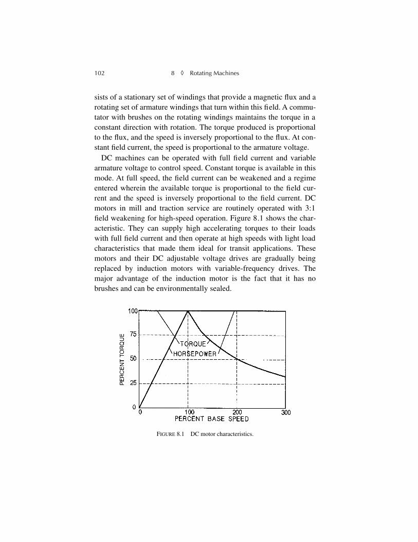
102 8
◊
Rotating Machines
sists of a stationary set of windings that provide a magnetic flux and arotating set of armature windings that turn within this field. A commu-tator with brushes on the rotating windings maintains the torque in aconstant direction with rotation. The torque produced is proportionalto the flux, and the speed is inversely proportional to the flux. At con-stant field current, the speed is proportional to the armature voltage.
DC machines can be operated with full field current and variablearmature voltage to control speed. Constant torque is available in thismode. At full speed, the field current can be weakened and a regimeentered wherein the available torque is proportional to the field cur-rent and the speed is inversely proportional to the field current. DCmotors in mill and traction service are routinely operated with 3:1field weakening for high-speed operation. Figure 8.1 shows the char-acteristic. They can supply high accelerating torques to their loadswith full field current and then operate at high speeds with light loadcharacteristics that made them ideal for transit applications. Thesemotors and their DC adjustable voltage drives are gradually beingreplaced by induction motors with variable-frequency drives. Themajor advantage of the induction motor is the fact that it has nobrushes and can be environmentally sealed.
FIGURE 8.1 DC motor characteristics.
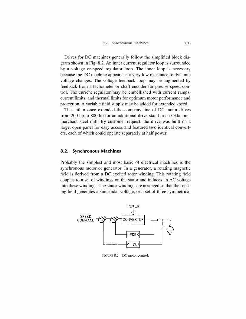
8.2. Synchronous Machines 103
Drives for DC machines generally follow the simplified block dia-gram shown in Fig. 8.2. An inner current regulator loop is surroundedby a voltage or speed regulator loop. The inner loop is necessarybecause the DC machine appears as a very low resistance to dynamicvoltage changes. The voltage feedback loop may be augmented byfeedback from a tachometer or shaft encoder for precise speed con-trol. The current regulator may be embellished with current ramps,current limits, and thermal limits for optimum motor performance andprotection. A variable field supply may be added for extended speed.
The author once extended the company line of DC motor drivesfrom 200 hp to 800 hp for an additional drive stand in an Oklahomamerchant steel mill. By customer request, the drive was built on alarge, open panel for easy access and featured two identical convert-ers, each of which could operate separately at half power.
8.2. Synchronous Machines
Probably the simplest and most basic of electrical machines is thesynchronous motor or generator. In a generator, a rotating magneticfield is derived from a DC excited rotor winding. This rotating fieldcouples to a set of windings on the stator and induces an AC voltageinto these windings. The stator windings are arranged so that the rotat-ing field generates a sinusoidal voltage, or a set of three symmetrical
FIGURE 8.2 DC motor control.
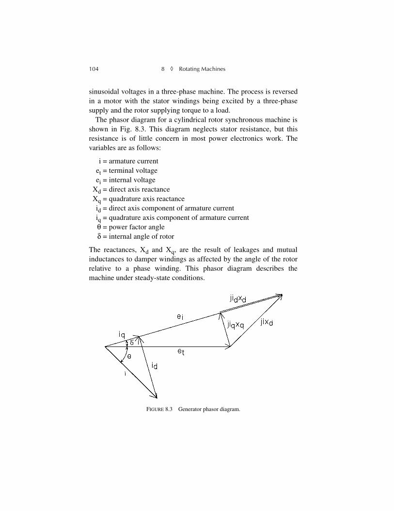
104 8
◊
Rotating Machines
sinusoidal voltages in a three-phase machine. The process is reversedin a motor with the stator windings being excited by a three-phasesupply and the rotor supplying torque to a load.
The phasor diagram for a cylindrical rotor synchronous machine isshown in Fig. 8.3. This diagram neglects stator resistance, but thisresistance is of little concern in most power electronics work. Thevariables are as follows:
i = armature currente
t
= terminal voltagee
i
= internal voltageX
d
= direct axis reactanceX
q
= quadrature axis reactancei
d
= direct axis component of armature currenti
q
= quadrature axis component of armature current
θ
= power factor angle
δ
= internal angle of rotor
The reactances, X
d
and X
q
, are the result of leakages and mutualinductances to damper windings as affected by the angle of the rotorrelative to a phase winding. This phasor diagram describes themachine under steady-state conditions.
FIGURE 8.3 Generator phasor diagram.
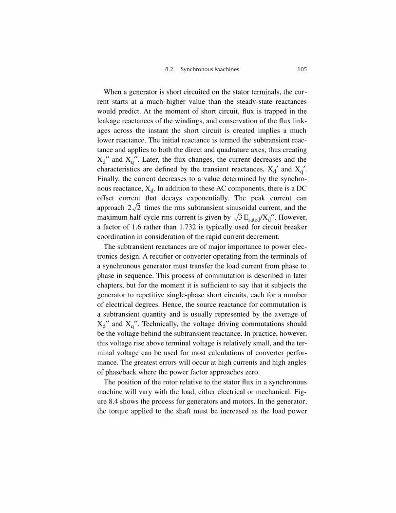
8.2. Synchronous Machines 105
When a generator is short circuited on the stator terminals, the cur-rent starts at a much higher value than the steady-state reactanceswould predict. At the moment of short circuit, flux is trapped in theleakage reactances of the windings, and conservation of the flux link-ages across the instant the short circuit is created implies a muchlower reactance. The initial reactance is termed the subtransient reac-tance and applies to both the direct and quadrature axes, thus creatingX
d
′′
and X
q
′′
. Later, the flux changes, the current decreases and thecharacteristics are defined by the transient reactances, X
d
′
and X
q
′
.Finally, the current decreases to a value determined by the synchro-nous reactance, X
d
. In addition to these AC components, there is a DCoffset current that decays exponentially. The peak current canapproach times the rms subtransient sinusoidal current, and themaximum half-cycle rms current is given by E
rated
/X
d
′′
. However,a factor of 1.6 rather than 1.732 is typically used for circuit breakercoordination in consideration of the rapid current decrement.
The subtransient reactances are of major importance to power elec-tronics design. A rectifier or converter operating from the terminals ofa synchronous generator must transfer the load current from phase tophase in sequence. This process of commutation is described in laterchapters, but for the moment it is sufficient to say that it subjects thegenerator to repetitive single-phase short circuits, each for a numberof electrical degrees. Hence, the source reactance for commutation isa subtransient quantity and is usually represented by the average ofX
d
′′
and X
q
′′
. Technically, the voltage driving commutations shouldbe the voltage behind the subtransient reactance. In practice, however,this voltage rise above terminal voltage is relatively small, and the ter-minal voltage can be used for most calculations of converter perfor-mance. The greatest errors will occur at high currents and high anglesof phaseback where the power factor approaches zero.
The position of the rotor relative to the stator flux in a synchronousmachine will vary with the load, either electrical or mechanical. Fig-ure 8.4 shows the process for generators and motors. In the generator,the torque applied to the shaft must be increased as the load power
2 23
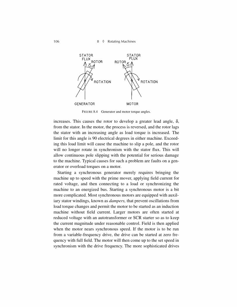
106 8
◊
Rotating Machines
increases. This causes the rotor to develop a greater lead angle,
δ
,from the stator. In the motor, the process is reversed, and the rotor lagsthe stator with an increasing angle as load torque is increased. Thelimit for this angle is 90 electrical degrees in either machine. Exceed-ing this load limit will cause the machine to slip a pole, and the rotorwill no longer rotate in synchronism with the stator flux. This willallow continuous pole slipping with the potential for serious damageto the machine. Typical causes for such a problem are faults on a gen-erator or overload torques on a motor.
Starting a synchronous generator merely requires bringing themachine up to speed with the prime mover, applying field current forrated voltage, and then connecting to a load or synchronizing themachine to an energized bus. Starting a synchronous motor is a bitmore complicated. Most synchronous motors are equipped with auxil-iary stator windings, known as
dampers,
that prevent oscillations fromload torque changes and permit the motor to be started as an inductionmachine without field current. Larger motors are often started atreduced voltage with an autotransformer or SCR starter so as to keepthe current magnitude under reasonable control. Field is then appliedwhen the motor nears synchronous speed. If the motor is to be runfrom a variable-frequency drive, the drive can be started at zero fre-quency with full field. The motor will then come up to the set speed insynchronism with the drive frequency. The more sophisticated drives
FIGURE 8.4 Generator and motor torque angles.

8.3. Induction (Asynchronous) Machines 107
will search out the initial rotor position by applying a small field exci-tation and observing the induced voltages in the stator phase wind-ings. The drive phase can then be adjusted so that there is no torquetransient or reverse rotation on starting.
Modern variable-frequency drives have enabled synchronousmotors to replace many of the large DC machines used in steel millsfor rapid reversing because of their ability to provide transient torquesof several times rated value. The drive must be able to determine thetorque angle and maintain a safe margin from pole slipping.
8.3. Induction (Asynchronous) Machines
The stator winding for an induction machine looks like the statorwinding on a synchronous machine. However, instead of an exter-nally energized field winding, the induction machine has a rotorwith, typically, copper or aluminum axial bars embedded in mag-netic laminations at the outer periphery of the rotor. By energizingthe stator windings with multiphase current, a rotating flux is cre-ated, just as in the synchronous motor. This flux induces currents inthe rotor bars and creates a torque reaction. The rotor must rotate atan electrical speed lower or higher than that of the stator to producethe eddy currents and torque. If the rotor speed is lower, it will pro-duce shaft torque to a load. If torque is applied to the shaft in thedirection of rotation, the motor can operate at a rotor frequencyhigher than synchronous and deliver electrical power from the stator.The difference between shaft speed and synchronous speed is knownas
slip
and is usually expressed as a percent or per unit of synchro-nous speed. The induction motor can be operated as an inductiongenerator with no external power if the excitation that provides therotational flux is supplied from a capacitor bank on the stator. Themachine will usually build up voltage self-excited from residual flux.However, it may be necessary to flash a voltage on the stator to startthe process. The capacitance can be adjusted to operate the machineat rated voltage.
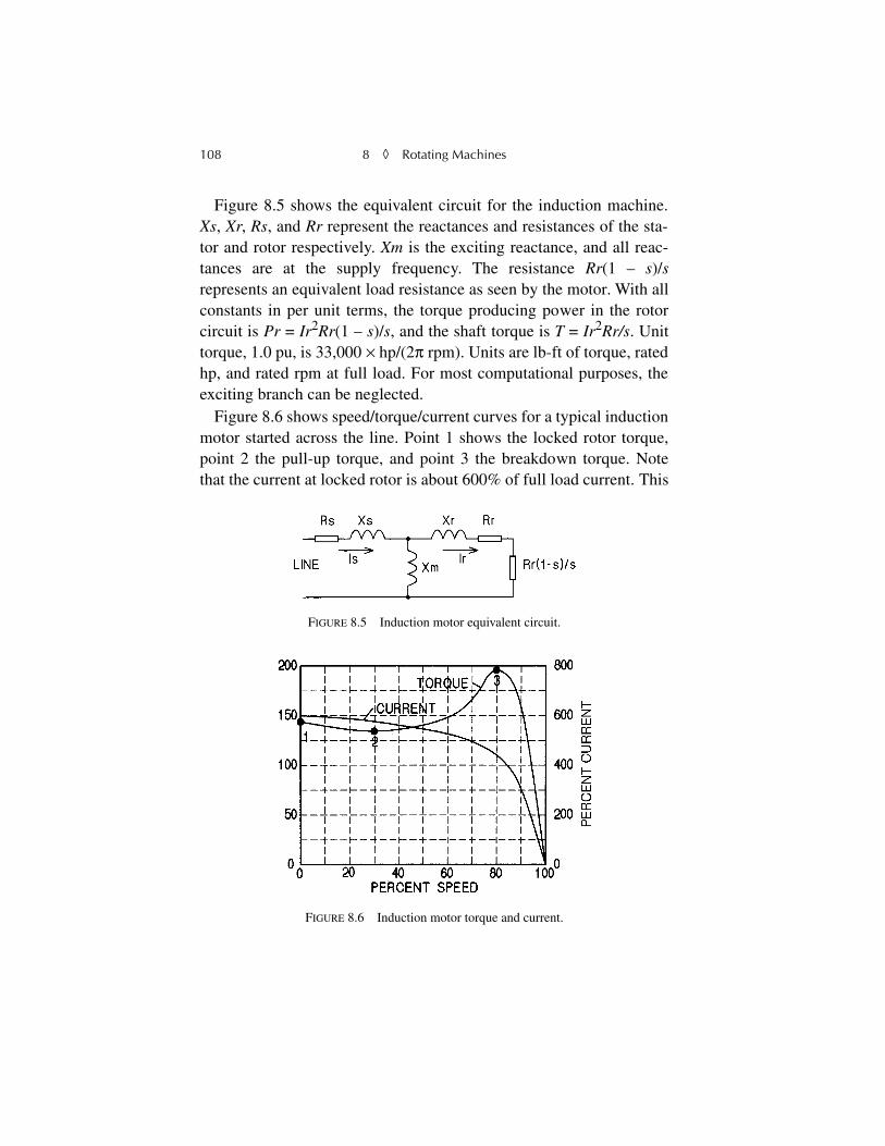
108 8
◊
Rotating Machines
Figure 8.5 shows the equivalent circuit for the induction machine.
Xs
,
Xr
,
Rs
, and
Rr
represent the reactances and resistances of the sta-tor and rotor respectively.
Xm
is the exciting reactance, and all reac-tances are at the supply frequency. The resistance
Rr
(1 –
s
)/
s
represents an equivalent load resistance as seen by the motor. With allconstants in per unit terms, the torque producing power in the rotorcircuit is
Pr
=
Ir
2
Rr
(1 –
s
)/
s
, and the shaft torque is
T
=
Ir
2
Rr/s
. Unittorque, 1.0 pu, is 33,000
×
hp/(2
π
rpm). Units are lb-ft of torque, ratedhp, and rated rpm at full load. For most computational purposes, theexciting branch can be neglected.
Figure 8.6 shows speed/torque/current curves for a typical inductionmotor started across the line. Point 1 shows the locked rotor torque,point 2 the pull-up torque, and point 3 the breakdown torque. Notethat the current at locked rotor is about 600% of full load current. This
FIGURE 8.5 Induction motor equivalent circuit.
FIGURE 8.6 Induction motor torque and current.
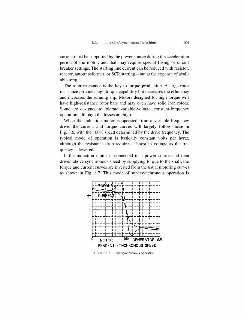
8.3. Induction (Asynchronous) Machines 109
current must be supported by the power source during the accelerationperiod of the motor, and that may require special fusing or circuitbreaker settings. The starting line current can be reduced with resistor,reactor, autotransformer, or SCR starting—but at the expense of avail-able torque.
The rotor resistance is the key to torque production. A large rotorresistance provides high torque capability but decreases the efficiencyand increases the running slip. Motors designed for high torque willhave high-resistance rotor bars and may even have solid iron rotors.Some are designed to tolerate variable-voltage, constant-frequencyoperation, although the losses are high.
When the induction motor is operated from a variable-frequencydrive, the current and torque curves will largely follow those inFig. 8.6, with the 100% speed determined by the drive frequency. Thetypical mode of operation is basically constant volts per hertz,although the resistance drop requires a boost in voltage as the fre-quency is lowered.
If the induction motor is connected to a power source and thendriven above synchronous speed by supplying torque to the shaft, thetorque and current curves are inverted from the usual motoring curvesas shown in Fig. 8.7. This mode of supersynchronous operation is
FIGURE 8.7 Supersynchronous operation.
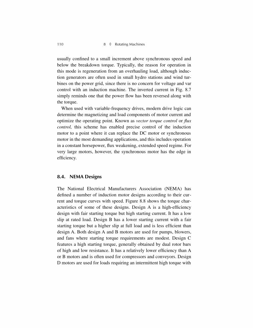
110 8
◊
Rotating Machines
usually confined to a small increment above synchronous speed andbelow the breakdown torque. Typically, the reason for operation inthis mode is regeneration from an overhauling load, although induc-tion generators are often used in small hydro stations and wind tur-bines on the power grid, since there is no concern for voltage and varcontrol with an induction machine. The inverted current in Fig. 8.7simply reminds one that the power flow has been reversed along withthe torque.
When used with variable-frequency drives, modern drive logic candetermine the magnetizing and load components of motor current andoptimize the operating point. Known as
vector torque control
or
fluxcontrol,
this scheme has enabled precise control of the inductionmotor to a point where it can replace the DC motor or synchronousmotor in the most demanding applications, and this includes operationin a constant horsepower, flux weakening, extended speed regime. Forvery large motors, however, the synchronous motor has the edge inefficiency.
8.4. NEMA Designs
The National Electrical Manufacturers Association (NEMA) hasdefined a number of induction motor designs according to their cur-rent and torque curves with speed. Figure 8.8 shows the torque char-acteristics of some of these designs. Design A is a high-efficiencydesign with fair starting torque but high starting current. It has a lowslip at rated load. Design B has a lower starting current with a fairstarting torque but a higher slip at full load and is less efficient thandesign A. Both design A and B motors are used for pumps, blowers,and fans where starting torque requirements are modest. Design Cfeatures a high starting torque, generally obtained by dual rotor barsof high and low resistance. It has a relatively lower efficiency than Aor B motors and is often used for compressors and conveyors. DesignD motors are used for loads requiring an intermittent high torque with
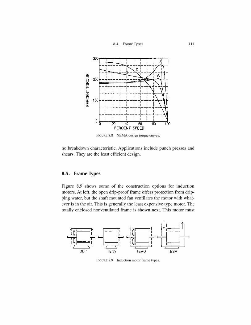
8.4. Frame Types 111
no breakdown characteristic. Applications include punch presses andshears. They are the least efficient design.
8.5. Frame Types
Figure 8.9 shows some of the construction options for inductionmotors. At left, the open drip-proof frame offers protection from drip-ping water, but the shaft mounted fan ventilates the motor with what-ever is in the air. This is generally the least expensive type motor. Thetotally enclosed nonventilated frame is shown next. This motor must
FIGURE 8.8 NEMA design torque curves.
FIGURE 8.9 Induction motor frame types.
112 8
◊
Rotating Machines
rely on radiation and natural convection from the frame for cooling,but it is not affected by corrosive or explosive fumes in the air. It isrelatively expensive and larger than the ODP frame for a given horse-power. In the totally enclosed air-over design, the cooling of theTENV motor is augmented by a shaft-mounted fan that blows air overthe frame. Finally, the totally enclosed, separately ventilated motor iscooled with externally supplied air.
8.6. Linear Motors
Although this chapter is titled
rotating machines
, an exception shouldbe made to introduce the linear induction motor. In principle, aninduction motor stator can be sawed open and then fanned out into astraight line. When excited with three-phase power, it will apply aforce parallel to the linear windings in an aluminum or copper plate inclose proximity. Replicating a set of windings in a line allows themotor to be extended mechanically as far as desired. By means ofSCR switches, coil sections can be switched in only when the plate isin the vicinity of the particular coil set to economize on the requiredpower. A system of this sort is currently being actively investigated inthe EMALS program, an electromagnetic aircraft launching systemsponsored by the U.S. Navy for new aircraft carriers. EMALS offersthe capability of controlling the applied accelerating force to accom-modate both drones and the largest carrier aircraft. Furthermore, itwill require less maintenance and operating manpower than the steamcatapults. The present EMALS program requires about 200 peak MWand 100 MJ from a stored energy generator. The generator output iscontrolled by a set of SCR converters to produce a variable-voltageDC bus that powers a set of inverters and coil switches for the linearmotor.
Yet another interesting application for a linear motor (of a sort) isthe rail gun. Figure 8.10 shows the nature of the system. When ashorting bar is placed across two current-carrying conductors, aLorentz force is produced that acts on the shorting bar. If the bar is

8.6. Linear Motors 113
free to move with a brush system to maintain contact with the conduc-tors, it will accelerate rapidly. Such systems are presently under devel-opment to provide weapons with hypervelocity projectiles.
The development challenges in this project are daunting. The short-ing bar must make good contact with the rails, yet the currents are inthe order of several MA. Rail erosion from arcing must be kept in rea-sonable bounds. When the projectile exits the rails, a short or termi-nating resistor must be used to limit the voltage from energy stored inthe rail inductances. Power must be supplied from rotational generatorenergy and SCR converters used to control the current. The systemmust ultimately be installed in a military vehicle of some sort wherespace and weight are severely limited. Despite all these difficulties, adevelopment system has been demonstrated, and work on this fasci-nating project continues at this time.
FIGURE 8.10 Elementary rail gun.

115
Chapter 9
Rectifiers and Converters
Despite the general acceptance and growth of AC power systems, theneed continued for DC in electrochemistry, variable speed motors,and traction systems. Although George Westinghouse demonstratedAC traction motors, they were operated at 25 Hz rather than the pre-vailing 60 Hz used for utility systems. Metropolitan transit systems,however, required DC for the traction motors. The New York subwaysystem generated and distributed 25-Hz power but ran the cars on DCthrough rotary converters. With the predominately 60 Hz power sys-tems, the problem became one of converting 60 Hz AC to DC. Theterms
rectifier
and
converter
are often used interchangeably to denotea system of any sort that converts AC to DC. Present-day usage seemsto favor
rectifier
to denote an uncontrolled conversion system and
converter
to denote a controlled system.
9.1. Early Rectifiers
Rotary converters, double wound, rotating synchronous machines,had been used on 25-Hz power to generate DC since the early days.The need for DC by some industries had influenced the choice of25 Hz for the initial generation at Niagara Falls because, in the earlydays of magnetic materials, it was difficult to make the rotary convert-
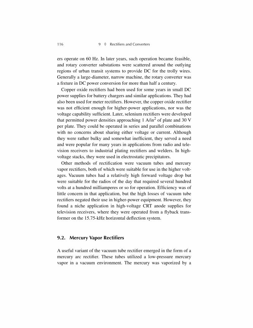
116 9
◊
Rectifiers and Converters
ers operate on 60 Hz. In later years, such operation became feasible,and rotary converter substations were scattered around the outlyingregions of urban transit systems to provide DC for the trolly wires.Generally a large-diameter, narrow machine, the rotary converter wasa fixture in DC power conversion for more than half a century.
Copper oxide rectifiers had been used for some years in small DCpower supplies for battery chargers and similar applications. They hadalso been used for meter rectifiers. However, the copper oxide rectifierwas not efficient enough for higher-power applications, nor was thevoltage capability sufficient. Later, selenium rectifiers were developedthat permitted power densities approaching 1 A/in
2
of plate and 30 Vper plate. They could be operated in series and parallel combinationswith no concerns about sharing either voltage or current. Althoughthey were rather bulky and somewhat inefficient, they served a needand were popular for many years in applications from radio and tele-vision receivers to industrial plating rectifiers and welders. In high-voltage stacks, they were used in electrostatic precipitators.
Other methods of rectification were vacuum tubes and mercuryvapor rectifiers, both of which were suitable for use in the higher volt-ages. Vacuum tubes had a relatively high forward voltage drop butwere suitable for the radios of the day that required several hundredvolts at a hundred milliamperes or so for operation. Efficiency was oflittle concern in that application, but the high losses of vacuum tuberectifiers negated their use in higher-power equipment. However, theyfound a niche application in high-voltage CRT anode supplies fortelevision receivers, where they were operated from a flyback trans-former on the 15.75-kHz horizontal deflection system.
9.2. Mercury Vapor Rectifiers
A useful variant of the vacuum tube rectifier emerged in the form of amercury arc rectifier. These tubes utilized a low-pressure mercuryvapor in a vacuum environment. The mercury was vaporized by a
9.1. Silicon Diodes—The Semiconductor Age 117
heated filamentary cathode. The voltage drop was typically around15 V, and they could be built for operation at several tens of kilovolts.As hot cathode tubes, they were widely used in communications,where they supplied DC voltages for most radio transmitters at powerlevels as high as 1 MW in voltages from 5 to 15 kV.
Very large rectifiers were made with evacuated glass and metalenclosures containing multiple anodes and a pool of liquid mercury.They were used with the double-wye interphase transformer circuitdescribed later to provide high currents for electroplating and DC ser-vice buses for metal processing mills. They also supplied high-current“pot lines” for the electrolytic reduction of aluminum and other met-als as well as chlorine production. A starter electrode vaporized themercury in these units, and the tanks were maintained at a low pres-sure by vacuum pumps.
Later developments included a sealed glass and metal enclosedhigh-current rectifier with an ignitor electrode that permitted it to actas a high-current switch. Sold under the trade name Ignitron
®
, theseunits became very popular and ruled the rectifier field until the devel-opment of solid-state technology in mid century.
9.3. Silicon Diodes—The Semiconductor Age
The now-familiar silicon diode grew out of the development of thepoint contact germanium transistor by Brattain and Bardeen at BellLaboratories in 1947. Later work in many laboratories resulted inalloyed junctions, higher current capabilities, and the transition fromgermanium to silicon. By 1960, silicon rectifiers were widely avail-able and coming into general use. Germanium power rectifiers wereavailable in large sizes, but their restricted temperature capabilitieslimited their use.
The advantage of silicon for diodes was that it could operate atjunction temperatures approaching 200°C. Their forward drop washigher than that of germanium diodes, but the higher temperature
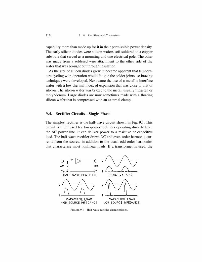
118 9
◊
Rectifiers and Converters
capability more than made up for it in their permissible power density.The early silicon diodes were silicon wafers soft soldered to a coppersubstrate that served as a mounting and one electrical pole. The otherwas made from a soldered wire attachment to the other side of thewafer that was brought out through insulation.
As the size of silicon diodes grew, it became apparent that tempera-ture cycling with operation would fatigue the solder joints, so brazingtechniques were developed. Next came the use of a metallic interfacewafer with a low thermal index of expansion that was close to that ofsilicon. The silicon wafer was brazed to the metal, usually tungsten ormolybdenum. Large diodes are now sometimes made with a floatingsilicon wafer that is compressed with an external clamp.
9.4. Rectifier Circuits—Single-Phase
The simplest rectifier is the half-wave circuit shown in Fig. 9.1. Thiscircuit is often used for low-power rectifiers operating directly fromthe AC power line. It can deliver power to a resistive or capacitiveload. The half-wave rectifier draws DC and even-order harmonic cur-rents from the source, in addition to the usual odd-order harmonicsthat characterize most nonlinear loads. If a transformer is used, the
FIGURE 9.1 Half-wave rectifier characteristics.
9.4. Rectifier Circuits—Single-Phase 119
DC component may saturate the iron, but a gapped core can allow fluxreset and prevent this.
Half-wave rectifiers are often used with filter capacitors to provide alow-ripple DC output. The capacitive load makes the line current con-duction angle decrease as shown in Fig. 9.1. High-frequency har-monic currents increase, and the apparent power factor, P/VA,decreases. The rectifier in this case is subjected to a peak reverse volt-age equal to the capacitor voltage plus the peak line voltage. Since thecapacitor usually is charged to near peak line voltage, the diode mustbe rated for repetitive operation at twice peak line voltage.
Although the half-wave circuit is widely used in switch-modepower supplies where the poor current waveform may not cause aproblem, an aggregation of such power supplies can have seriouseffects on the power system in, for example, a data processing center.Single-phase loads with such current distortion have a high percent-age of triplen harmonics, both even and odd order—3, 6, 9, 12, 15, 18,21, …. These triplen harmonic currents are additive in the neutral of athree-phase distribution system, and the neutral current can approachtwice the line current. Oversized neutral conductors are required.Equipments that cause DC components in the supply lines of electricutilities are not permitted by IEEE 519, but the DC components ofhalf-wave power supplies do not pass beyond the first transformerthey encounter. However, they may cause the core of the transformerto saturate.
The full-wave, center-tapped rectifier shown in Fig. 9.2 was widelyused in the days of radio, because the two rectifying elements couldbe contained in the same vacuum tube. It is still popular for low-volt-age supplies, since there is only a single rectifier element in serieswith the load. However, many of these simple rectifiers have beensuperseded by switch-mode units that are much smaller and lighterbecause of their high-frequency transformer. These are described inChapter 13.
The secondary sections in this circuit carry half-wave currents withan rms value of 50% of peak over a full cycle. With a primary voltage
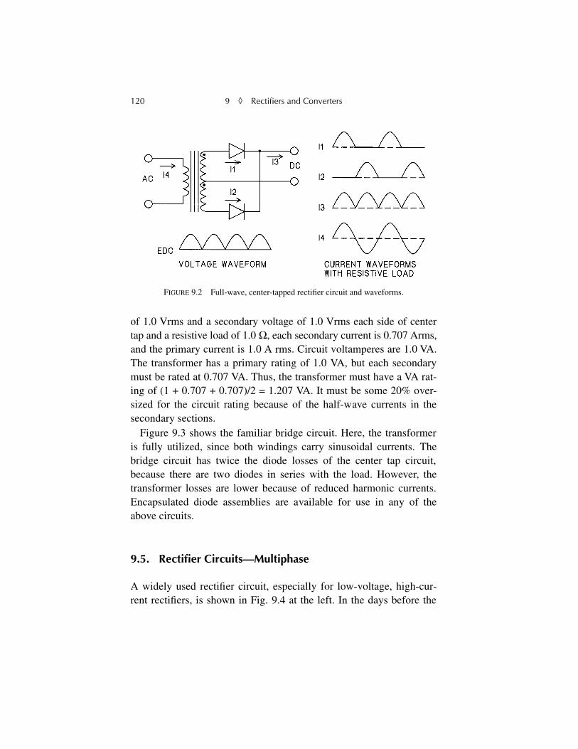
120 9
◊
Rectifiers and Converters
of 1.0 Vrms and a secondary voltage of 1.0 Vrms each side of centertap and a resistive load of 1.0
Ω
, each secondary current is 0.707 Arms,and the primary current is 1.0 A rms. Circuit voltamperes are 1.0 VA.The transformer has a primary rating of 1.0 VA, but each secondarymust be rated at 0.707 VA. Thus, the transformer must have a VA rat-ing of (1 + 0.707 + 0.707)/2 = 1.207 VA. It must be some 20% over-sized for the circuit rating because of the half-wave currents in thesecondary sections.
Figure 9.3 shows the familiar bridge circuit. Here, the transformeris fully utilized, since both windings carry sinusoidal currents. Thebridge circuit has twice the diode losses of the center tap circuit,because there are two diodes in series with the load. However, thetransformer losses are lower because of reduced harmonic currents.Encapsulated diode assemblies are available for use in any of theabove circuits.
9.5. Rectifier Circuits—Multiphase
A widely used rectifier circuit, especially for low-voltage, high-cur-rent rectifiers, is shown in Fig. 9.4 at the left. In the days before the
FIGURE 9.2 Full-wave, center-tapped rectifier circuit and waveforms.
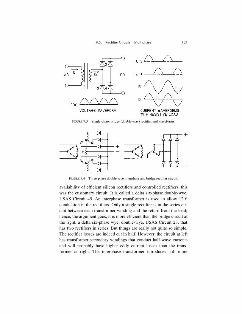
9.5. Rectifier Circuits—Multiphase 121
availability of efficient silicon rectifiers and controlled rectifiers, thiswas the customary circuit. It is called a delta six-phase double-wye,USAS Circuit 45. An interphase transformer is used to allow 120°conduction in the rectifiers. Only a single rectifier is in the series cir-cuit between each transformer winding and the return from the load;hence, the argument goes, it is more efficient than the bridge circuit atthe right, a delta six-phase wye, double-wye, USAS Circuit 23, thathas two rectifiers in series. But things are really not quite so simple.The rectifier losses are indeed cut in half. However, the circuit at lefthas transformer secondary windings that conduct half-wave currentsand will probably have higher eddy current losses than the trans-former at right. The interphase transformer introduces still more
FIGURE 9.3 Single-phase bridge (double-way) rectifier and waveforms.
FIGURE 9.4 Three-phase double-wye interphase and bridge rectifier circuit.
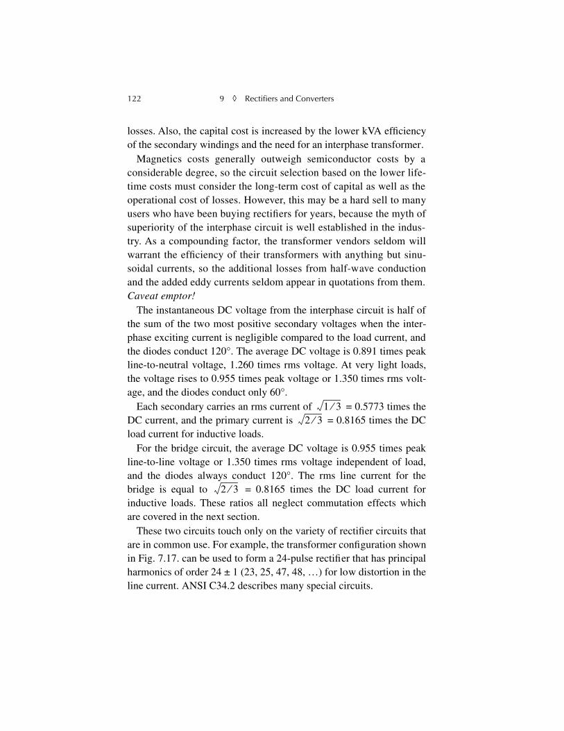
122 9
◊
Rectifiers and Converters
losses. Also, the capital cost is increased by the lower kVA efficiencyof the secondary windings and the need for an interphase transformer.
Magnetics costs generally outweigh semiconductor costs by aconsiderable degree, so the circuit selection based on the lower life-time costs must consider the long-term cost of capital as well as theoperational cost of losses. However, this may be a hard sell to manyusers who have been buying rectifiers for years, because the myth ofsuperiority of the interphase circuit is well established in the indus-try. As a compounding factor, the transformer vendors seldom willwarrant the efficiency of their transformers with anything but sinu-soidal currents, so the additional losses from half-wave conductionand the added eddy currents seldom appear in quotations from them.
Caveat emptor!
The instantaneous DC voltage from the interphase circuit is half ofthe sum of the two most positive secondary voltages when the inter-phase exciting current is negligible compared to the load current, andthe diodes conduct 120°. The average DC voltage is 0.891 times peakline-to-neutral voltage, 1.260 times rms voltage. At very light loads,the voltage rises to 0.955 times peak voltage or 1.350 times rms volt-age, and the diodes conduct only 60°.
Each secondary carries an rms current of = 0.5773 times theDC current, and the primary current is = 0.8165 times the DCload current for inductive loads.
For the bridge circuit, the average DC voltage is 0.955 times peakline-to-line voltage or 1.350 times rms voltage independent of load,and the diodes always conduct 120°. The rms line current for thebridge is equal to = 0.8165 times the DC load current forinductive loads. These ratios all neglect commutation effects whichare covered in the next section.
These two circuits touch only on the variety of rectifier circuits thatare in common use. For example, the transformer configuration shownin Fig. 7.17. can be used to form a 24-pulse rectifier that has principalharmonics of order 24 ± 1 (23, 25, 47, 48, …) for low distortion in theline current. ANSI C34.2 describes many special circuits.
1 3⁄2 3⁄
2 3⁄
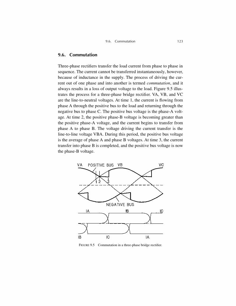
9.6. Commutation 123
9.6. Commutation
Three-phase rectifiers transfer the load current from phase to phase insequence. The current cannot be transferred instantaneously, however,because of inductance in the supply. The process of driving the cur-rent out of one phase and into another is termed
commutation
, and italways results in a loss of output voltage to the load. Figure 9.5 illus-trates the process for a three-phase bridge rectifier. VA, VB, and VCare the line-to-neutral voltages. At time 1, the current is flowing fromphase A through the positive bus to the load and returning through thenegative bus to phase C. The positive bus voltage is the phase-A volt-age. At time 2, the positive phase-B voltage is becoming greater thanthe positive phase-A voltage, and the current begins to transfer fromphase A to phase B. The voltage driving the current transfer is theline-to-line voltage VBA. During this period, the positive bus voltageis the average of phase A and phase B voltages. At time 3, the currenttransfer into phase B is completed, and the positive bus voltage is nowthe phase-B voltage.
FIGURE 9.5 Commutation in a three-phase bridge rectifier.
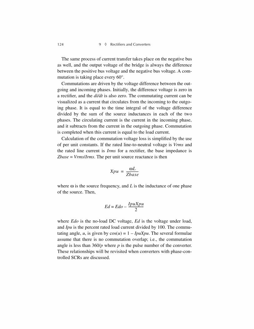
124 9
◊
Rectifiers and Converters
The same process of current transfer takes place on the negative busas well, and the output voltage of the bridge is always the differencebetween the positive bus voltage and the negative bus voltage. A com-mutation is taking place every 60°.
Commutations are driven by the voltage difference between the out-going and incoming phases. Initially, the difference voltage is zero ina rectifier, and the
di/dt
is also zero. The commutating current can bevisualized as a current that circulates from the incoming to the outgo-ing phase. It is equal to the time integral of the voltage differencedivided by the sum of the source inductances in each of the twophases. The circulating current is the current in the incoming phase,and it subtracts from the current in the outgoing phase. Commutationis completed when this current is equal to the load current.
Calculation of the commutation voltage loss is simplified by the useof per unit constants. If the rated line-to-neutral voltage is
Vrms
andthe rated line current is
Irms
for a rectifier, the base impedance is
Zbase
=
Vrms
/
Irms
. The per unit source reactance is then
where
ω
is the source frequency, and
L
is the inductance of one phaseof the source. Then,
Ed
=
Edo
–
where
Edo
is the no-load DC voltage,
Ed
is the voltage under load,and
Ipu
is the percent rated load current divided by 100. The commu-tating angle,
u
, is given by cos(
u
) = 1 –
IpuXpu
. The several formulaeassume that there is no commutation overlap; i.e., the commutationangle is less than 360/
p
where
p
is the pulse number of the converter.These relationships will be revisited when converters with phase-con-trolled SCRs are discussed.
XpuωL
Zbase---------------=
IpuXpu2
-------------------
125
Chapter 10
Phase Control
The invention of mercury arc rectifiers in the 1920s made it possibleto control a load voltage by varying the conduction angle of a rectifierwith a low-power control ignitor. Later years produced the gas-filledthyratron that extended this capability to lower-power equipments.Motor drives, welders, controllers, and a host of other applicationsfollowed, but the limitations in reliability and efficiency, coupled withthe relatively high cost of this equipment, precluded widespread use.The market was confined to special applications where the advantagesoutweighed the disadvantages.
A second approach to phase control involved magnetics in the formof saturable reactors and magnetic amplifiers. Saturable reactors hadbeen used for many years in applications that could tolerate a rela-tively slow response time, and advances in metallurgy brought“square loop” magnetic materials that improved the characteristics ofthese devices. In the early 1950s, the combination of improved mag-netics and low-leakage selenium rectifiers had advanced the art ofmagnetic amplifiers to a point where they were used in autopilots formilitary aircraft, but their slow response and high weight were farfrom ideal.
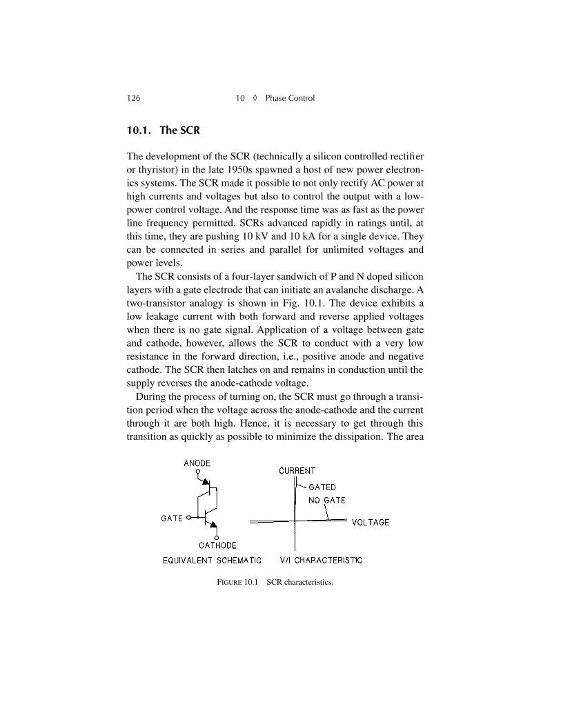
126 10
◊
Phase Control
10.1. The SCR
The development of the SCR (technically a silicon controlled rectifieror thyristor) in the late 1950s spawned a host of new power electron-ics systems. The SCR made it possible to not only rectify AC power athigh currents and voltages but also to control the output with a low-power control voltage. And the response time was as fast as the powerline frequency permitted. SCRs advanced rapidly in ratings until, atthis time, they are pushing 10 kV and 10 kA for a single device. Theycan be connected in series and parallel for unlimited voltages andpower levels.
The SCR consists of a four-layer sandwich of P and N doped siliconlayers with a gate electrode that can initiate an avalanche discharge. Atwo-transistor analogy is shown in Fig. 10.1. The device exhibits alow leakage current with both forward and reverse applied voltageswhen there is no gate signal. Application of a voltage between gateand cathode, however, allows the SCR to conduct with a very lowresistance in the forward direction, i.e., positive anode and negativecathode. The SCR then latches on and remains in conduction until thesupply reverses the anode-cathode voltage.
During the process of turning on, the SCR must go through a transi-tion period when the voltage across the anode-cathode and the currentthrough it are both high. Hence, it is necessary to get through thistransition as quickly as possible to minimize the dissipation. The area
FIGURE 10.1 SCR characteristics.
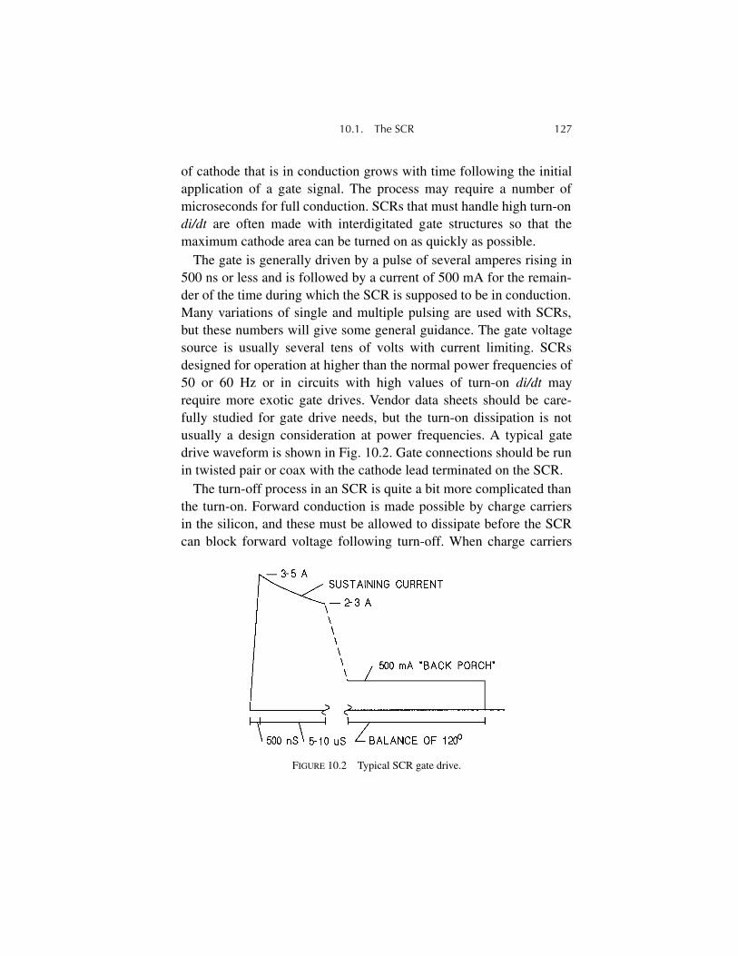
10.1. The SCR 127
of cathode that is in conduction grows with time following the initialapplication of a gate signal. The process may require a number ofmicroseconds for full conduction. SCRs that must handle high turn-on
di/dt
are often made with interdigitated gate structures so that themaximum cathode area can be turned on as quickly as possible.
The gate is generally driven by a pulse of several amperes rising in500 ns or less and is followed by a current of 500 mA for the remain-der of the time during which the SCR is supposed to be in conduction.Many variations of single and multiple pulsing are used with SCRs,but these numbers will give some general guidance. The gate voltagesource is usually several tens of volts with current limiting. SCRsdesigned for operation at higher than the normal power frequencies of50 or 60 Hz or in circuits with high values of turn-on
di/dt
mayrequire more exotic gate drives. Vendor data sheets should be care-fully studied for gate drive needs, but the turn-on dissipation is notusually a design consideration at power frequencies. A typical gatedrive waveform is shown in Fig. 10.2. Gate connections should be runin twisted pair or coax with the cathode lead terminated on the SCR.
The turn-off process in an SCR is quite a bit more complicated thanthe turn-on. Forward conduction is made possible by charge carriersin the silicon, and these must be allowed to dissipate before the SCRcan block forward voltage following turn-off. When charge carriers
FIGURE 10.2 Typical SCR gate drive.
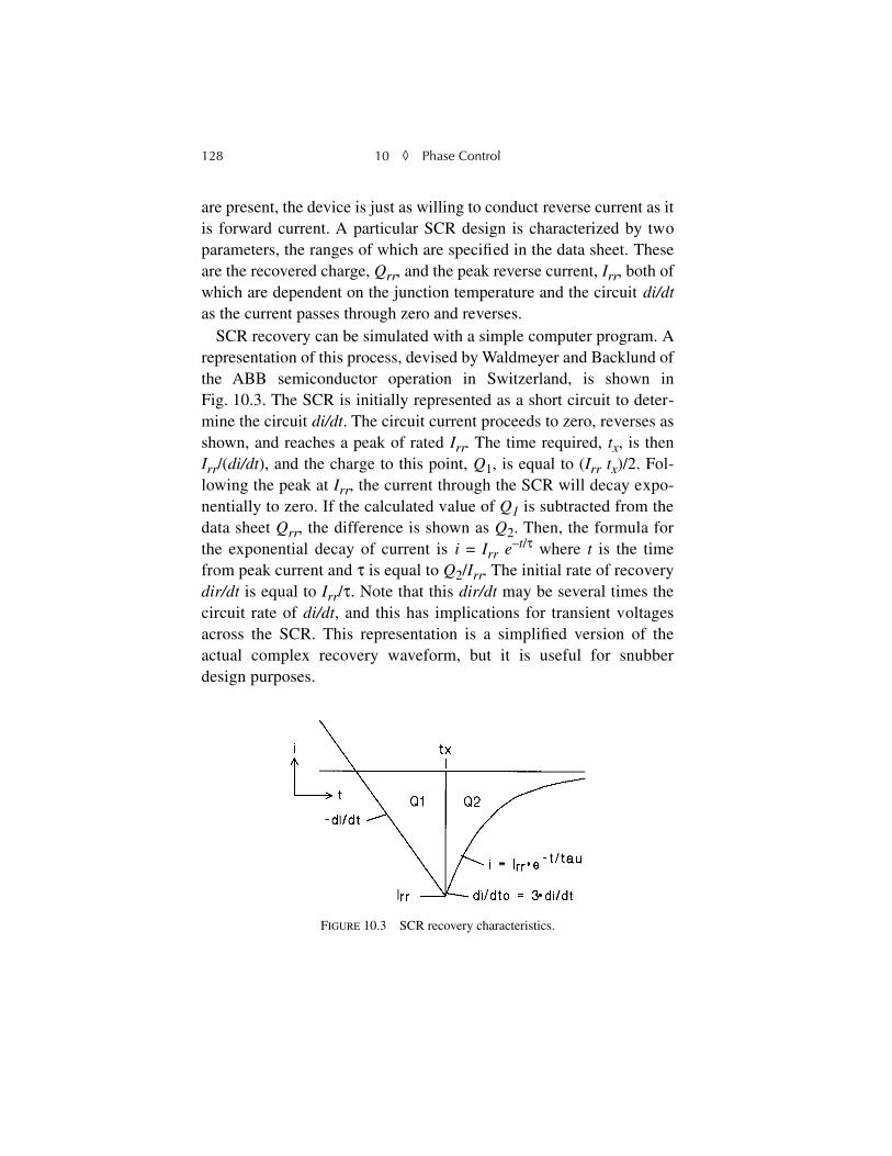
128 10
◊
Phase Control
are present, the device is just as willing to conduct reverse current as itis forward current. A particular SCR design is characterized by twoparameters, the ranges of which are specified in the data sheet. Theseare the recovered charge,
Q
rr
, and the peak reverse current,
I
rr
, both ofwhich are dependent on the junction temperature and the circuit
di/dt
as the current passes through zero and reverses.SCR recovery can be simulated with a simple computer program. A
representation of this process, devised by Waldmeyer and Backlund ofthe ABB semiconductor operation in Switzerland, is shown inFig. 10.3. The SCR is initially represented as a short circuit to deter-mine the circuit
di/dt
. The circuit current proceeds to zero, reverses asshown, and reaches a peak of rated
I
rr
. The time required,
t
x
, is then
I
rr
/(
di/dt
), and the charge to this point,
Q
1
, is equal to (
I
rr
t
x
)/2. Fol-lowing the peak at
I
rr
, the current through the SCR will decay expo-nentially to zero. If the calculated value of
Q
1
is subtracted from thedata sheet
Q
rr
, the difference is shown as
Q
2
. Then, the formula forthe exponential decay of current is
i
=
I
rr
e
–
t
/
τ
where
t
is the timefrom peak current and
τ
is equal to
Q
2
/
I
rr
. The initial rate of recovery
dir/dt
is equal to
I
rr
/
τ
. Note that this
dir/dt
may be several times thecircuit rate of
di/dt
, and this has implications for transient voltagesacross the SCR. This representation is a simplified version of theactual complex recovery waveform, but it is useful for snubberdesign purposes.
FIGURE 10.3 SCR recovery characteristics.
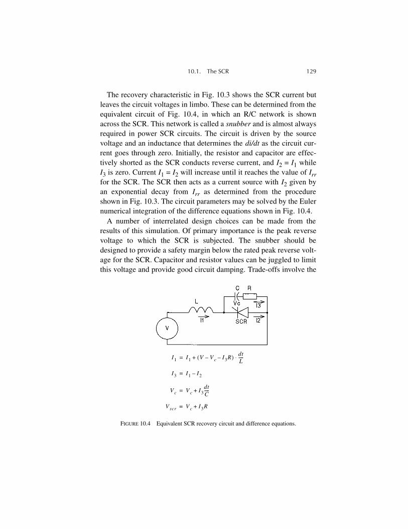
10.1. The SCR 129
The recovery characteristic in Fig. 10.3 shows the SCR current butleaves the circuit voltages in limbo. These can be determined from theequivalent circuit of Fig. 10.4, in which an R/C network is shownacross the SCR. This network is called a
snubber
and is almost alwaysrequired in power SCR circuits. The circuit is driven by the sourcevoltage and an inductance that determines the
di/dt
as the circuit cur-rent goes through zero. Initially, the resistor and capacitor are effec-tively shorted as the SCR conducts reverse current, and
I
2
=
I
1
while
I
3
is zero. Current
I
1
=
I
2
will increase until it reaches the value of
I
rr
for the SCR. The SCR then acts as a current source with
I
2
given byan exponential decay from
I
rr
as determined from the procedureshown in Fig. 10.3. The circuit parameters may be solved by the Eulernumerical integration of the difference equations shown in Fig. 10.4.
A number of interrelated design choices can be made from theresults of this simulation. Of primary importance is the peak reversevoltage to which the SCR is subjected. The snubber should bedesigned to provide a safety margin below the rated peak reverse volt-age for the SCR. Capacitor and resistor values can be juggled to limitthis voltage and provide good circuit damping. Trade-offs involve the
FIGURE 10.4 Equivalent SCR recovery circuit and difference equations.
I1 I1 V V c I3R––( ) dtL-----⋅+=
I3 I1 I2–=
V c V c I3dtC-----+=
V scr V c I3R+=
130 10
◊
Phase Control
rather considerable cost of the capacitor, which must be an extendedfoil type, and the dissipation of the resistor, which must be a nonin-ductive type. A secondary consideration may be the turn-on
di/dt
limitof the SCR, since it must discharge the capacitor through the resistor.The resistor dissipation must include this discharge energy as well asthe turn-off dissipation from the recovery simulation. Note that manycircuits involve a number of snubber networks that will interact, andthe R/C values for the simulation must be the equivalent shunt valuesas seen by the recovering SCR. For the three-phase full wave con-verter, the equivalent resistor,
R
eq
, is given by
R
eq
= 3
R
/5, where
R
isthe actual resistor on each SCR, and
C
eq
, the equivalent capacitorvalue is
C
eq
= 5
C
/3. These R/C values can then be adjusted by theinverse relationship to define the actual values for the snubber compo-nents. The snubbers should mounted as close to the SCR as possibleto minimize stray inductance.
Some vendors define the recovery characteristic by an “s” factor thatcan be used to determine the current decay time constant. The maxi-mum recovery
dir/dt
is equal to the circuit
di/dt
divided by the s factor,typical values for which are 0.33 for SCRs and as low as 0.1 for somediodes. The exponential time constant,
τ
, is equal to
I
rr
/(
dir/dt
) asbefore.
It is important to coordinate the maximum SCR recovery voltagewith the voltage rating of MOV devices used for transient protection.The recovery voltage cannot be allowed to reach the MOV clampingvoltage, because this would cause overheating and failure of the MOV.The MOV is rated for occasional transients only, and it cannot with-stand exposure to repetitive transients such as those of SCR recovery.
Recovery dissipation for the SCR can be determined by integratingits Irr*Vr product from the simulation. This is usually a nontrivialvalue for large SCRs, even at power frequencies. An estimate of theselosses is included in the vendor’s data sheet for allowable currents atvarious firing angles at power frequencies, but a more serious evalua-tion is often warranted, especially in higher-frequency operation,since switching losses are proportional to the source frequency.
10.1. Forward Drop 131
10.2. Forward Drop
SCRs have a nonlinear forward drop that is usually the major determi-nant of the allowable load current in a circuit. The rated currents oftencan be obtained from a series of curves most vendors show for variousphaseback angles. If the operating conditions do not correspond withany published curves, the losses must be calculated from the currentwaveform and the forward drop. A given SCR in a three-phase bridgeconducts only about 120°, neglecting commutation, per cycle. It isimportant to calculate the power from the integrated V I product usingthe actual current waveform. This power can then be divided by threeto get the average value over the cycle. The loss power cannot bedetermined by using the average current.
Two identical semiconductors with different duty cycles can becompared for losses. The first is carrying pulses of 100 A on a 10%duty cycle with an average current of 10 A. The second is carrying10 A on a 100% duty cycle. A forward resistance drop of 0.1 Ω isassumed. The first dissipates 1000 W on a 10% duty cycle for 100 Waverage. The second dissipates only 10 W. The peak junction tempera-ture rise of the first will be more than ten times that of the second.
The preceding discussion is a rather condensed treatise on the careand feeding of SCRs, and it is suggested that the reader study theavailable technical literature as well as vendor data sheets for morespecific design information.
10.3. SCR Circuits—AC Switches
Figure 10.5 shows two SCRs connected back-to-back in a single-phase AC switch configuration, each handling one polarity of the ACsource voltage. The fraction of each half-cycle of the voltage that isdelivered to the load is controlled by the timing of the gate signals.The angle from the positive going zero crossing of the voltage to theapplication of the gate signal is the delay angle or firing angle, α.Figure 10.6 shows the output voltage and current waveforms for vari-ous delay angles and load power factors.
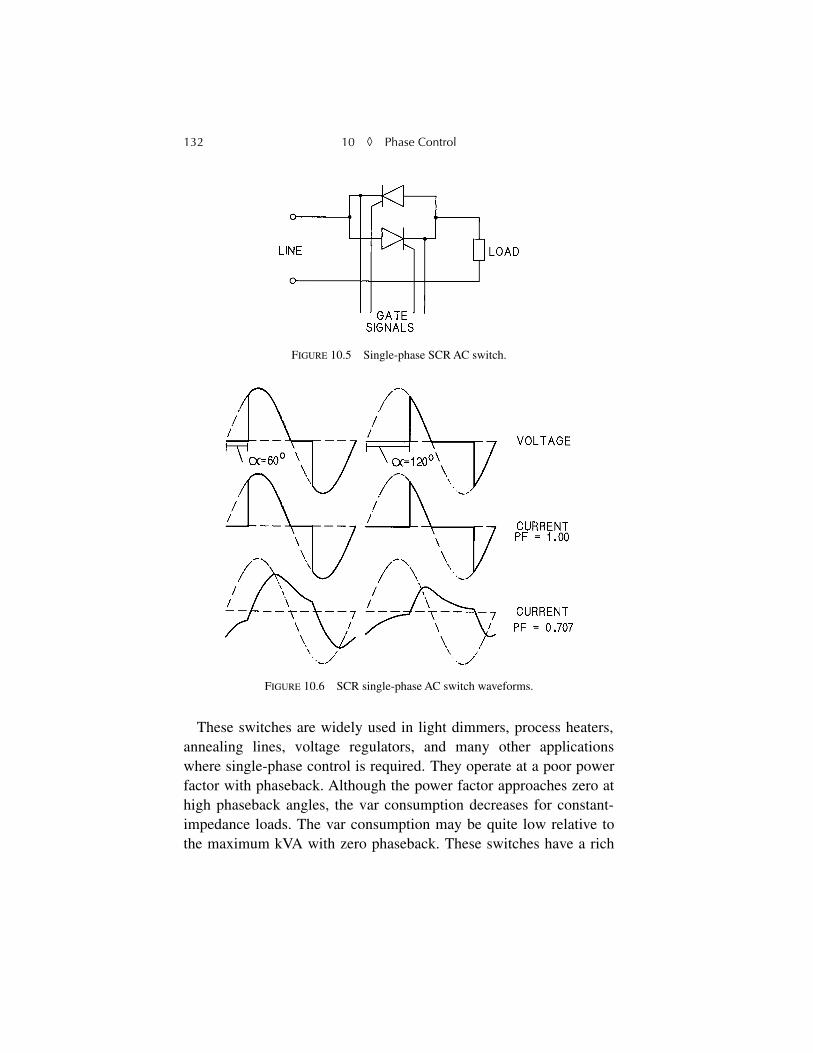
132 10 ◊ Phase Control
These switches are widely used in light dimmers, process heaters,annealing lines, voltage regulators, and many other applicationswhere single-phase control is required. They operate at a poor powerfactor with phaseback. Although the power factor approaches zero athigh phaseback angles, the var consumption decreases for constant-impedance loads. The var consumption may be quite low relative tothe maximum kVA with zero phaseback. These switches have a rich
FIGURE 10.5 Single-phase SCR AC switch.
FIGURE 10.6 SCR single-phase AC switch waveforms.
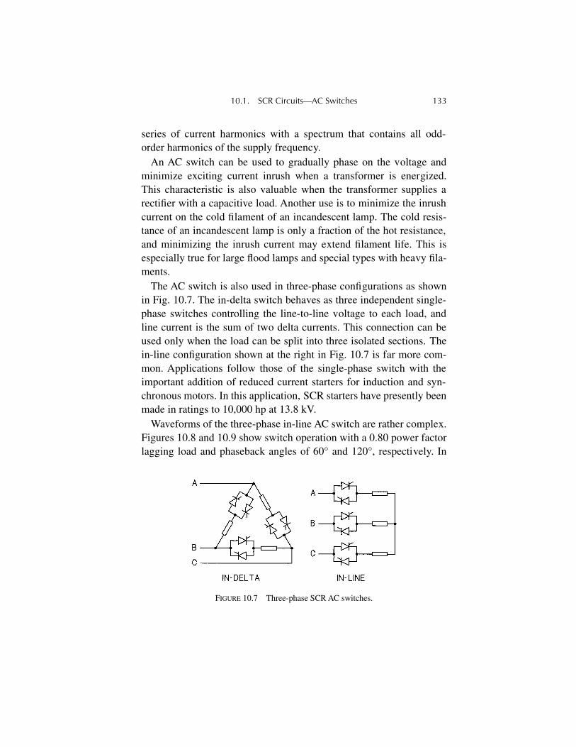
10.1. SCR Circuits—AC Switches 133
series of current harmonics with a spectrum that contains all odd-order harmonics of the supply frequency.
An AC switch can be used to gradually phase on the voltage andminimize exciting current inrush when a transformer is energized.This characteristic is also valuable when the transformer supplies arectifier with a capacitive load. Another use is to minimize the inrushcurrent on the cold filament of an incandescent lamp. The cold resis-tance of an incandescent lamp is only a fraction of the hot resistance,and minimizing the inrush current may extend filament life. This isespecially true for large flood lamps and special types with heavy fila-ments.
The AC switch is also used in three-phase configurations as shownin Fig. 10.7. The in-delta switch behaves as three independent single-phase switches controlling the line-to-line voltage to each load, andline current is the sum of two delta currents. This connection can beused only when the load can be split into three isolated sections. Thein-line configuration shown at the right in Fig. 10.7 is far more com-mon. Applications follow those of the single-phase switch with theimportant addition of reduced current starters for induction and syn-chronous motors. In this application, SCR starters have presently beenmade in ratings to 10,000 hp at 13.8 kV.
Waveforms of the three-phase in-line AC switch are rather complex.Figures 10.8 and 10.9 show switch operation with a 0.80 power factorlagging load and phaseback angles of 60° and 120°, respectively. In
FIGURE 10.7 Three-phase SCR AC switches.
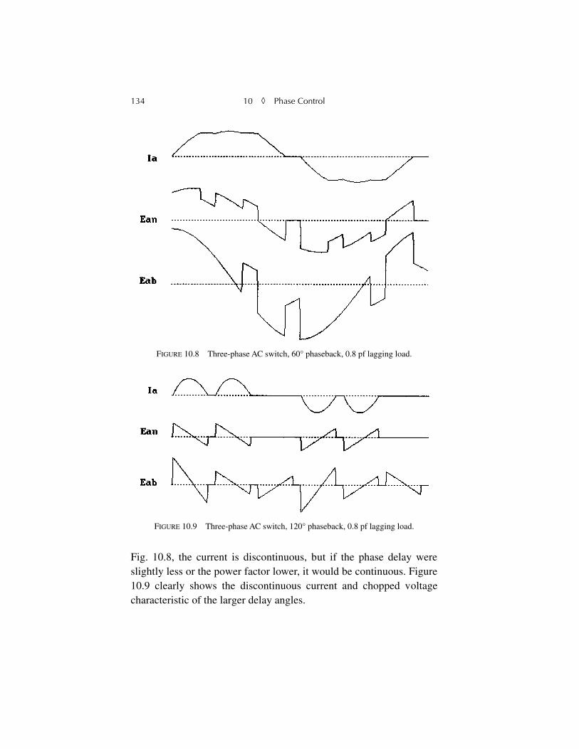
134 10 ◊ Phase Control
Fig. 10.8, the current is discontinuous, but if the phase delay wereslightly less or the power factor lower, it would be continuous. Figure10.9 clearly shows the discontinuous current and chopped voltagecharacteristic of the larger delay angles.
FIGURE 10.8 Three-phase AC switch, 60° phaseback, 0.8 pf lagging load.
FIGURE 10.9 Three-phase AC switch, 120° phaseback, 0.8 pf lagging load.

10.4. SCR Motor Starters 135
10.4. SCR Motor Starters
These waveforms are similar to those encountered with reduced cur-rent motor starters, although the induction motors usually have alower power factor on starting. Induction motors started across theline will draw initial currents of five or six times full load current.These high currents may cause problems with lamp flicker or voltagesags on other critical equipment connected to the same feeder. SCRstarters can reduce these problems—but at the expense of a reducedstarting torque on the motor. Torque is proportional to the square ofthe motor current, so a reduction in current to 50% of normal line cur-rent reduces the starting torque to only 25%. However, many loads,such as centrifugal fans and pumps, can start with these low torquesbecause, except for friction losses, their torques tend to increase as thesquare of the speed.
The combination of a low motor power factor and a large phasebackangle for current control means the SCR starter may present a verylow power factor to the feeder and thereby aggravate the voltage drop.Furthermore, the high harmonic content of the current may exceedallowable limits by the utility. One solution to both problems is to usepower factor correction capacitors coupled with one or more seriestuning inductors to improve power factor and divert harmonic currentsfrom the feeder. The capacitors may be switched in and out as requiredto keep the voltage within acceptable limits. If sufficient capacitors areused to maintain bus voltage at maximum starting current, they mustbe switched out to avoid overvoltages at normal running currents.
SCR starters are usually operated at a constant current equal to theminimum value required to satisfy the load torque requirements. Anadvantage of these starters is that the regulated current can be rampedup to the regulated level so that there is no sudden current demand onthe feeder, and the voltage drop is gradual. A gradual reduction inlamp brightness is much less objectionable psychologically than asudden drop.
Figure 10.10 shows the starting characteristics of a 2500-hp induc-tion motor driving a centrifugal pump. The current has been linearly
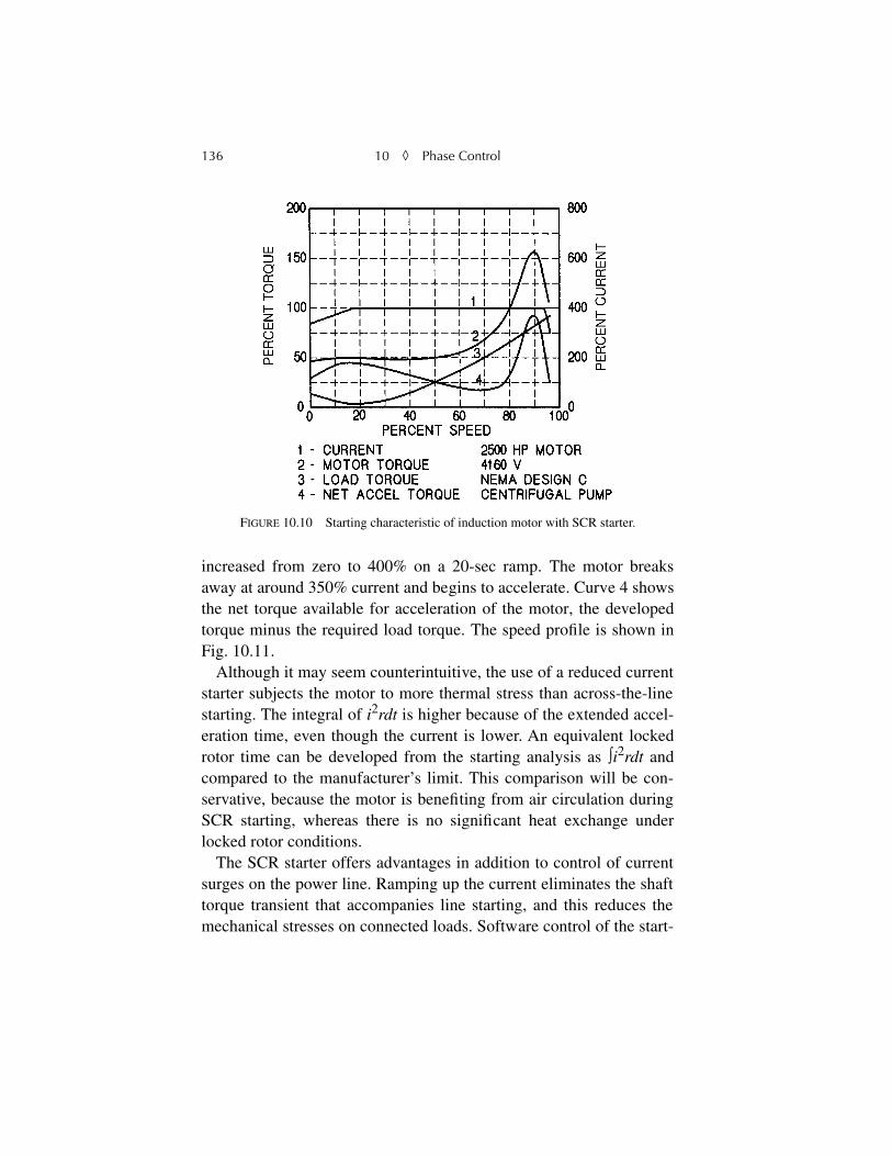
136 10 ◊ Phase Control
increased from zero to 400% on a 20-sec ramp. The motor breaksaway at around 350% current and begins to accelerate. Curve 4 showsthe net torque available for acceleration of the motor, the developedtorque minus the required load torque. The speed profile is shown inFig. 10.11.
Although it may seem counterintuitive, the use of a reduced currentstarter subjects the motor to more thermal stress than across-the-linestarting. The integral of i2rdt is higher because of the extended accel-eration time, even though the current is lower. An equivalent lockedrotor time can be developed from the starting analysis as ∫i2rdt andcompared to the manufacturer’s limit. This comparison will be con-servative, because the motor is benefiting from air circulation duringSCR starting, whereas there is no significant heat exchange underlocked rotor conditions.
The SCR starter offers advantages in addition to control of currentsurges on the power line. Ramping up the current eliminates the shafttorque transient that accompanies line starting, and this reduces themechanical stresses on connected loads. Software control of the start-
FIGURE 10.10 Starting characteristic of induction motor with SCR starter.
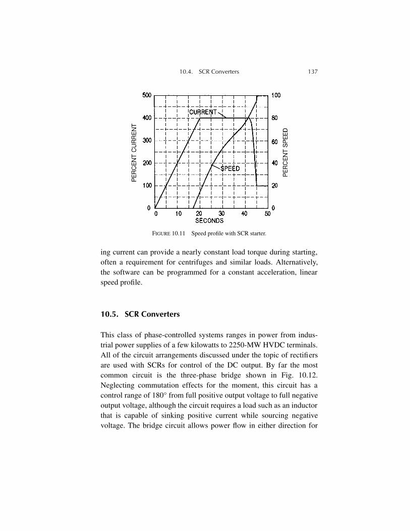
10.4. SCR Converters 137
ing current can provide a nearly constant load torque during starting,often a requirement for centrifuges and similar loads. Alternatively,the software can be programmed for a constant acceleration, linearspeed profile.
10.5. SCR Converters
This class of phase-controlled systems ranges in power from indus-trial power supplies of a few kilowatts to 2250-MW HVDC terminals.All of the circuit arrangements discussed under the topic of rectifiersare used with SCRs for control of the DC output. By far the mostcommon circuit is the three-phase bridge shown in Fig. 10.12.Neglecting commutation effects for the moment, this circuit has acontrol range of 180° from full positive output voltage to full negativeoutput voltage, although the circuit requires a load such as an inductorthat is capable of sinking positive current while sourcing negativevoltage. The bridge circuit allows power flow in either direction for
FIGURE 10.11 Speed profile with SCR starter.
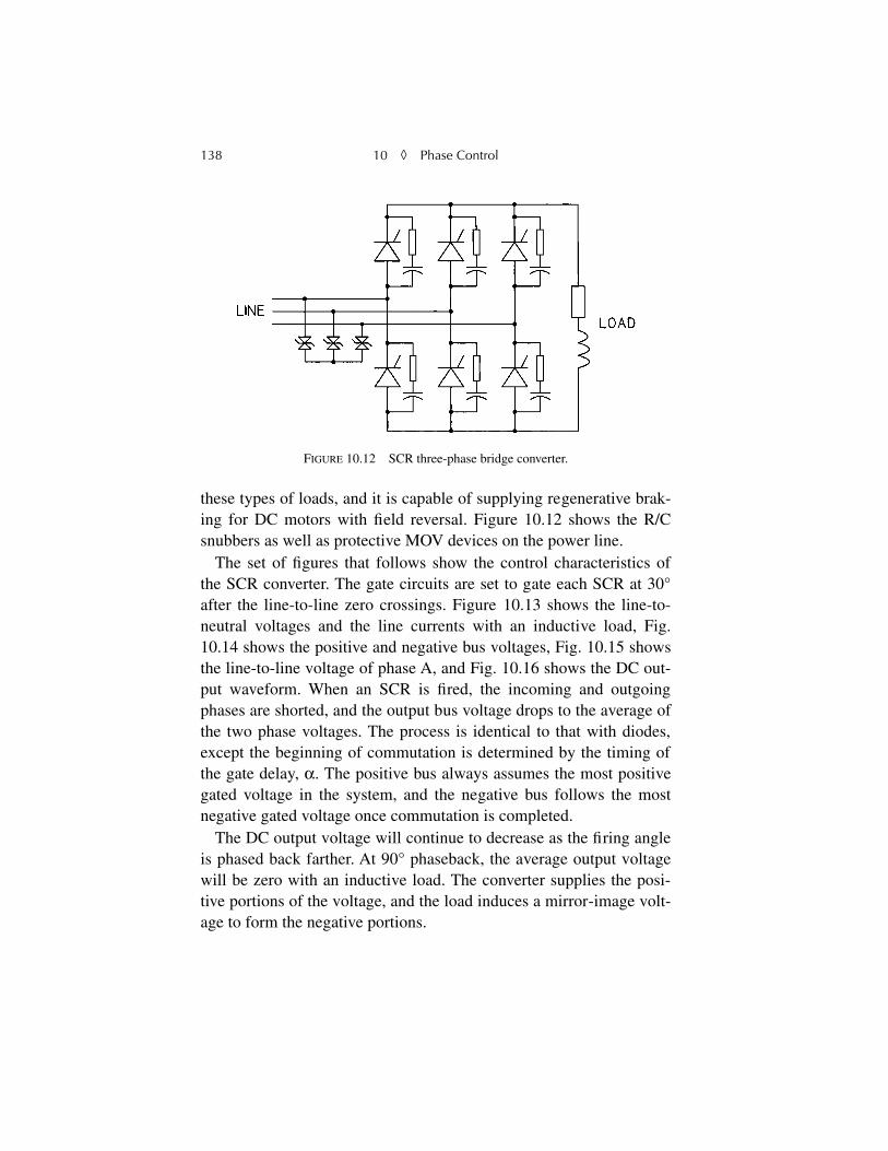
138 10 ◊ Phase Control
these types of loads, and it is capable of supplying regenerative brak-ing for DC motors with field reversal. Figure 10.12 shows the R/Csnubbers as well as protective MOV devices on the power line.
The set of figures that follows show the control characteristics ofthe SCR converter. The gate circuits are set to gate each SCR at 30°after the line-to-line zero crossings. Figure 10.13 shows the line-to-neutral voltages and the line currents with an inductive load, Fig.10.14 shows the positive and negative bus voltages, Fig. 10.15 showsthe line-to-line voltage of phase A, and Fig. 10.16 shows the DC out-put waveform. When an SCR is fired, the incoming and outgoingphases are shorted, and the output bus voltage drops to the average ofthe two phase voltages. The process is identical to that with diodes,except the beginning of commutation is determined by the timing ofthe gate delay, α. The positive bus always assumes the most positivegated voltage in the system, and the negative bus follows the mostnegative gated voltage once commutation is completed.
The DC output voltage will continue to decrease as the firing angleis phased back farther. At 90° phaseback, the average output voltagewill be zero with an inductive load. The converter supplies the posi-tive portions of the voltage, and the load induces a mirror-image volt-age to form the negative portions.
FIGURE 10.12 SCR three-phase bridge converter.
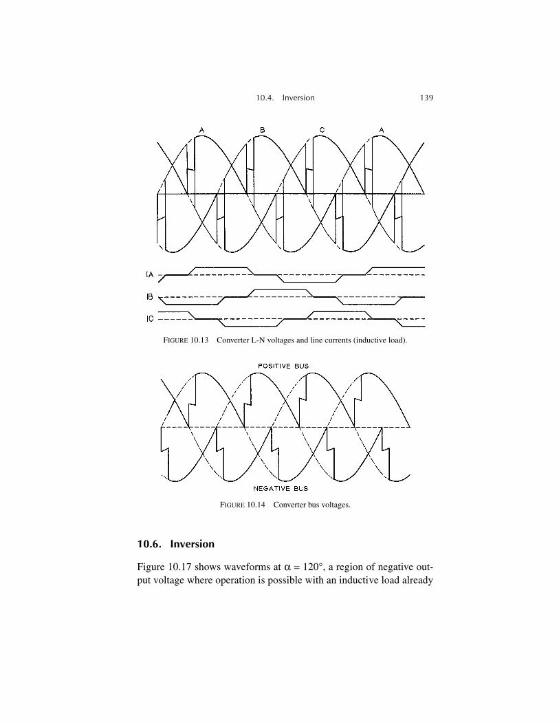
10.4. Inversion 139
10.6. Inversion
Figure 10.17 shows waveforms at α = 120°, a region of negative out-put voltage where operation is possible with an inductive load already
FIGURE 10.13 Converter L-N voltages and line currents (inductive load).
FIGURE 10.14 Converter bus voltages.
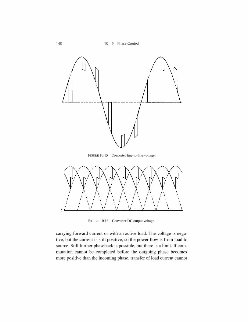
140 10 ◊ Phase Control
carrying forward current or with an active load. The voltage is nega-tive, but the current is still positive, so the power flow is from load tosource. Still further phaseback is possible, but there is a limit. If com-mutation cannot be completed before the outgoing phase becomesmore positive than the incoming phase, transfer of load current cannot
FIGURE 10.15 Converter line-to-line voltage.
FIGURE 10.16 Converter DC output voltage.
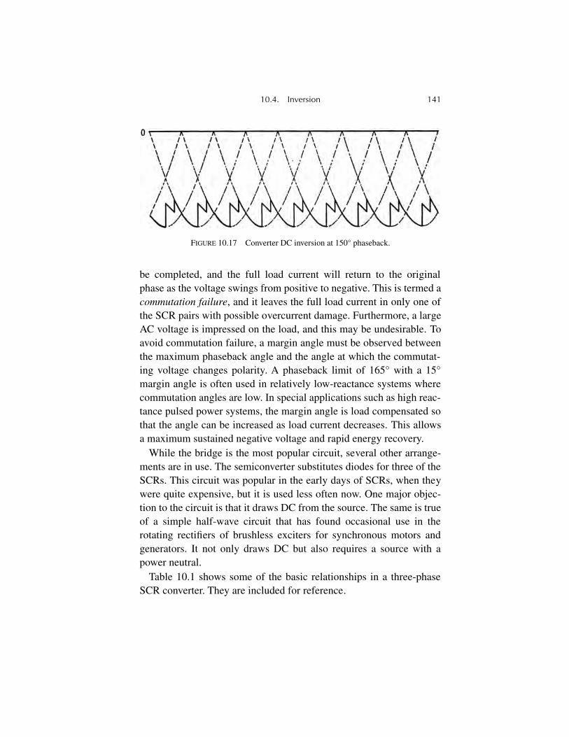
10.4. Inversion 141
be completed, and the full load current will return to the originalphase as the voltage swings from positive to negative. This is termed acommutation failure, and it leaves the full load current in only one ofthe SCR pairs with possible overcurrent damage. Furthermore, a largeAC voltage is impressed on the load, and this may be undesirable. Toavoid commutation failure, a margin angle must be observed betweenthe maximum phaseback angle and the angle at which the commutat-ing voltage changes polarity. A phaseback limit of 165° with a 15°margin angle is often used in relatively low-reactance systems wherecommutation angles are low. In special applications such as high reac-tance pulsed power systems, the margin angle is load compensated sothat the angle can be increased as load current decreases. This allowsa maximum sustained negative voltage and rapid energy recovery.
While the bridge is the most popular circuit, several other arrange-ments are in use. The semiconverter substitutes diodes for three of theSCRs. This circuit was popular in the early days of SCRs, when theywere quite expensive, but it is used less often now. One major objec-tion to the circuit is that it draws DC from the source. The same is trueof a simple half-wave circuit that has found occasional use in therotating rectifiers of brushless exciters for synchronous motors andgenerators. It not only draws DC but also requires a source with apower neutral.
Table 10.1 shows some of the basic relationships in a three-phaseSCR converter. They are included for reference.
FIGURE 10.17 Converter DC inversion at 150° phaseback.
142 10 ◊ Phase Control
10.7. Gate Drive Circuits
Many arrangements have been used to derive the phase references forSCR gate drives. These include phase shifters, phase locked loops,ramp intercepts, cosine intercepts, and programmable counters,among others. Most can be implemented in either hardware or soft-ware. A simple R/C phase shifter may be suitable when a limitedrange of phase control is satisfactory, although cascaded sections willprovide a larger range. The programmable counter relies on a high-frequency reference signal that is initiated at a reference point in theline voltage. The control then counts cycles of the reference to estab-lish a time delay which, of course, relates to phase delay of line volt-age. There will be a phase jitter in the gate drive if the referencefrequency is not synchronized to the line, but this can be made assmall as desired by increasing the reference frequency. A phaselocked loop gate drive can lock the reference frequency to the line bymeans of counters and a phase comparator.
A reference signal gated from a single phase can be used to estab-lish the six gate signals required for a three-phase SCR bridge.Although simple to implement, this may lead to some asymmetry inoutput if the supply phases are not balanced. The use of three refer-ences and three separate drive signals is preferred. All of these phas-ing systems have the disadvantage of a nonlinear transfer function ofcontrol voltage to bridge voltage since the delay angle is proportional
TABLE 10.1 Converter Equations
where Edo = no-load DC voltageEd = unloaded DC voltage
Ipu = per unit load currentXpu = per unit reactance of one phase
u = commutating angleα = phaseback anglepf = displacement power factor
Ed EdoIpuXpu
2-------------------–= u( )cos α( )cos IpuXpu–= p f α u
2---+⎝ ⎠
⎛ ⎞cos≈
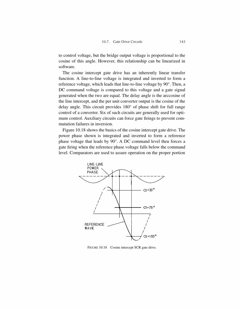
10.7. Gate Drive Circuits 143
to control voltage, but the bridge output voltage is proportional to thecosine of this angle. However, this relationship can be linearized insoftware.
The cosine intercept gate drive has an inherently linear transferfunction. A line-to-line voltage is integrated and inverted to form areference voltage, which leads that line-to-line voltage by 90°. Then, aDC command voltage is compared to this voltage and a gate signalgenerated when the two are equal. The delay angle is the arccosine ofthe line intercept, and the per unit converter output is the cosine of thedelay angle. This circuit provides 180° of phase shift for full rangecontrol of a converter. Six of such circuits are generally used for opti-mum control. Auxiliary circuits can force gate firings to prevent com-mutation failures in inversion.
Figure 10.18 shows the basics of the cosine intercept gate drive. Thepower phase shown is integrated and inverted to form a referencephase voltage that leads by 90°. A DC command level then forces agate firing when the reference phase voltage falls below the commandlevel. Comparators are used to assure operation on the proper portion
FIGURE 10.18 Cosine intercept SCR gate drive.
144 10 ◊ Phase Control
of the reference wave. Example DC command levels resulting indelays of 30°, 75°, and 150° are shown. If the power voltage rises, thereference voltage rises proportionally, and the intercept occurs later intime for a constant command level. Thus, the output voltage isreduced by phase delay as it tends to rise from the source voltageincrease. The output is self-compensating and maintains a constantvoltage.
Another major advantage of the cosine intercept circuit is that thereference voltage is derived by integrating a line voltage. Thus, a veryhigh degree of noise immunity is obtained. A large noise signalmerely results in a minor kink in the response linearity. The cosineintercept gate drive even tolerates commutation notches in the linevoltage. This is a distinct advantage over gating systems that require avoltage zero crossing for phase synchronization.
Another system of gate control that was employed on a generatorthat had to operate over a wide range of speed and frequency was touse a rotary encoder on the generator shaft to establish the internalangle. The terminal voltage for gate control was then synthesizedfrom this angle, the field excitation, machine parameters, and loadcurrent.
If the reader will excuse a brief departure from theory, a scene fromsome years ago may prove amusing. The author’s company was nego-tiating with a potential customer for a large, pulsed SCR converter.The customer was concerned about the ability of the cosine interceptgate drives to cope with a supply voltage that was seriously distortedby other converters on the line. A young engineer in the author’sgroup had set up an impressive demonstration to soothe the concernsof the customer and the customer’s consultant. With all the dignitariespresent, he threw the switch to power the several converters involved.At that precise moment, a small electrolytic capacitor decided on self-immolation and took off across the lab with a loud bang, trailing anever-longer spiral tail of aluminum foil. Fortunately, the customerlaughed it off, and the order was secured after minor repairs to thedemo equipment.
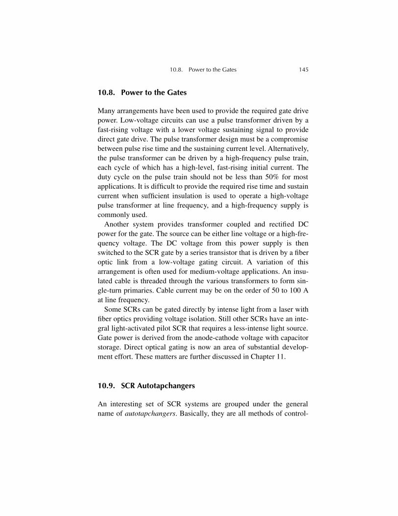
10.8. Power to the Gates 145
10.8. Power to the Gates
Many arrangements have been used to provide the required gate drivepower. Low-voltage circuits can use a pulse transformer driven by afast-rising voltage with a lower voltage sustaining signal to providedirect gate drive. The pulse transformer design must be a compromisebetween pulse rise time and the sustaining current level. Alternatively,the pulse transformer can be driven by a high-frequency pulse train,each cycle of which has a high-level, fast-rising initial current. Theduty cycle on the pulse train should not be less than 50% for mostapplications. It is difficult to provide the required rise time and sustaincurrent when sufficient insulation is used to operate a high-voltagepulse transformer at line frequency, and a high-frequency supply iscommonly used.
Another system provides transformer coupled and rectified DCpower for the gate. The source can be either line voltage or a high-fre-quency voltage. The DC voltage from this power supply is thenswitched to the SCR gate by a series transistor that is driven by a fiberoptic link from a low-voltage gating circuit. A variation of thisarrangement is often used for medium-voltage applications. An insu-lated cable is threaded through the various transformers to form sin-gle-turn primaries. Cable current may be on the order of 50 to 100 Aat line frequency.
Some SCRs can be gated directly by intense light from a laser withfiber optics providing voltage isolation. Still other SCRs have an inte-gral light-activated pilot SCR that requires a less-intense light source.Gate power is derived from the anode-cathode voltage with capacitorstorage. Direct optical gating is now an area of substantial develop-ment effort. These matters are further discussed in Chapter 11.
10.9. SCR Autotapchangers
An interesting set of SCR systems are grouped under the generalname of autotapchangers. Basically, they are all methods of control-
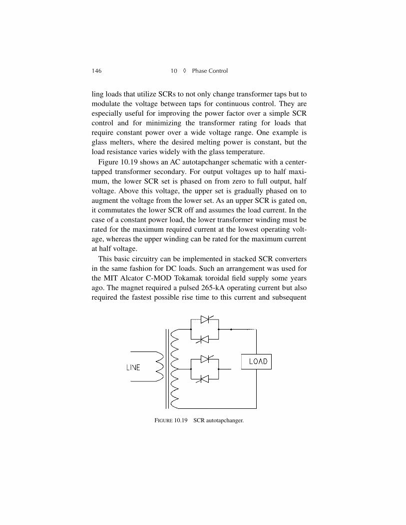
146 10 ◊ Phase Control
ling loads that utilize SCRs to not only change transformer taps but tomodulate the voltage between taps for continuous control. They areespecially useful for improving the power factor over a simple SCRcontrol and for minimizing the transformer rating for loads thatrequire constant power over a wide voltage range. One example isglass melters, where the desired melting power is constant, but theload resistance varies widely with the glass temperature.
Figure 10.19 shows an AC autotapchanger schematic with a center-tapped transformer secondary. For output voltages up to half maxi-mum, the lower SCR set is phased on from zero to full output, halfvoltage. Above this voltage, the upper set is gradually phased on toaugment the voltage from the lower set. As an upper SCR is gated on,it commutates the lower SCR off and assumes the load current. In thecase of a constant power load, the lower transformer winding must berated for the maximum required current at the lowest operating volt-age, whereas the upper winding can be rated for the maximum currentat half voltage.
This basic circuitry can be implemented in stacked SCR convertersin the same fashion for DC loads. Such an arrangement was used forthe MIT Alcator C-MOD Tokamak toroidal field supply some yearsago. The magnet required a pulsed 265-kA operating current but alsorequired the fastest possible rise time to this current and subsequent
FIGURE 10.19 SCR autotapchanger.
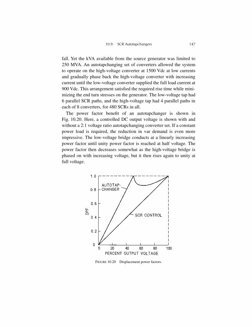
10.9. SCR Autotapchangers 147
fall. Yet the kVA available from the source generator was limited to250 MVA. An autotapchanging set of converters allowed the systemto operate on the high-voltage converter at 1500 Vdc at low currentsand gradually phase back the high-voltage converter with increasingcurrent until the low-voltage converter supplied the full load current at900 Vdc. This arrangement satisfied the required rise time while mini-mizing the end turn stresses on the generator. The low-voltage tap had6 parallel SCR paths, and the high-voltage tap had 4 parallel paths ineach of 8 converters, for 480 SCRs in all.
The power factor benefit of an autotapchanger is shown inFig. 10.20. Here, a controlled DC output voltage is shown with andwithout a 2:1 voltage ratio autotapchanging converter set. If a constantpower load is required, the reduction in var demand is even moreimpressive. The low-voltage bridge conducts at a linearly increasingpower factor until unity power factor is reached at half voltage. Thepower factor then decreases somewhat as the high-voltage bridge isphased on with increasing voltage, but it then rises again to unity atfull voltage.
FIGURE 10.20 Displacement power factors.
148 10 ◊ Phase Control
10.10. SCR DC Motor Drives
DC motor drives were an early application of phase-controlled con-verters. Regeneration can be obtained with a single bridge converterand a polarity-reversing field system. However, the response time ispoor and unsuited to the requirements for rapid regeneration andreversing in steel mill roll drives. The use of two bridges in an inverseparallel connection allows full reversing and regeneration by means ofarmature control. If the bridges are directly paralleled, one must bedisabled at all times to avoid a short circuit. The use of reactors tocouple the two bridges allows them to be gated simultaneously withthe reactors supporting the differences in their ripple voltages so longas a DC component is not present in both. If one is gated at angle α,the other is gated slightly behind 180° – α. The schematic for such adual converter arrangement is shown in Fig. 10.21.
The reactors can be either air core or iron core. This circuit allows asmooth transition between positive and negative motor current, animportant attribute for an optimum control loop response.
10.11. SCR AC Motor Drives
An early and rugged SCR AC motor drive consisted of an SCR DCconverter, a large inductor, and a set of six SCRs in a force-commu-
FIGURE 10.21 Reversing, regenerative SCR DC motor drive.
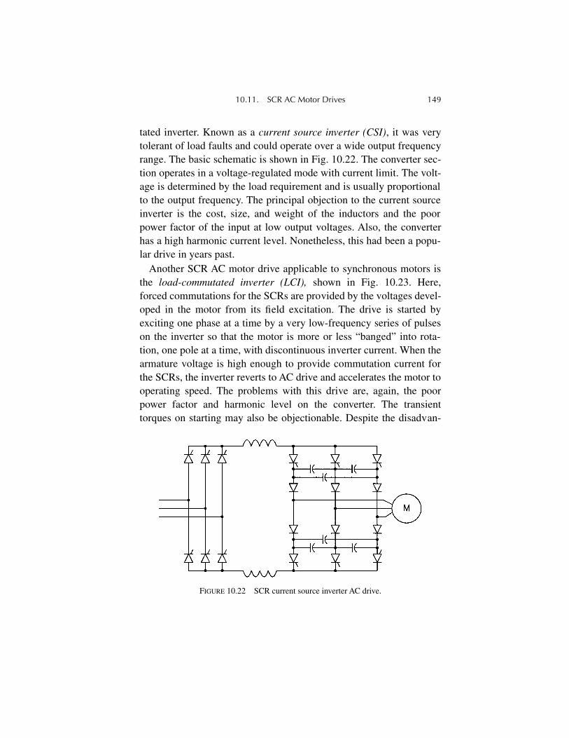
10.11. SCR AC Motor Drives 149
tated inverter. Known as a current source inverter (CSI), it was verytolerant of load faults and could operate over a wide output frequencyrange. The basic schematic is shown in Fig. 10.22. The converter sec-tion operates in a voltage-regulated mode with current limit. The volt-age is determined by the load requirement and is usually proportionalto the output frequency. The principal objection to the current sourceinverter is the cost, size, and weight of the inductors and the poorpower factor of the input at low output voltages. Also, the converterhas a high harmonic current level. Nonetheless, this had been a popu-lar drive in years past.
Another SCR AC motor drive applicable to synchronous motors isthe load-commutated inverter (LCI), shown in Fig. 10.23. Here,forced commutations for the SCRs are provided by the voltages devel-oped in the motor from its field excitation. The drive is started byexciting one phase at a time by a very low-frequency series of pulseson the inverter so that the motor is more or less “banged” into rota-tion, one pole at a time, with discontinuous inverter current. When thearmature voltage is high enough to provide commutation current forthe SCRs, the inverter reverts to AC drive and accelerates the motor tooperating speed. The problems with this drive are, again, the poorpower factor and harmonic level on the converter. The transienttorques on starting may also be objectionable. Despite the disadvan-
FIGURE 10.22 SCR current source inverter AC drive.
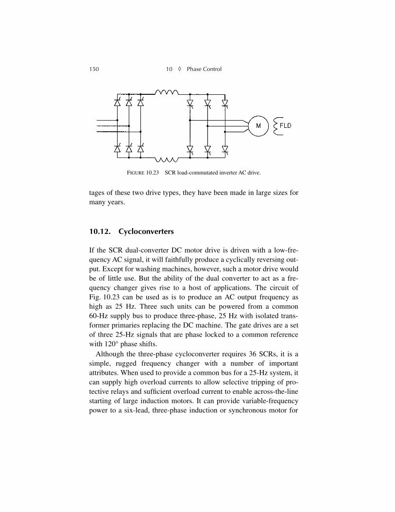
150 10 ◊ Phase Control
tages of these two drive types, they have been made in large sizes formany years.
10.12. Cycloconverters
If the SCR dual-converter DC motor drive is driven with a low-fre-quency AC signal, it will faithfully produce a cyclically reversing out-put. Except for washing machines, however, such a motor drive wouldbe of little use. But the ability of the dual converter to act as a fre-quency changer gives rise to a host of applications. The circuit ofFig. 10.23 can be used as is to produce an AC output frequency ashigh as 25 Hz. Three such units can be powered from a common60-Hz supply bus to produce three-phase, 25 Hz with isolated trans-former primaries replacing the DC machine. The gate drives are a setof three 25-Hz signals that are phase locked to a common referencewith 120° phase shifts.
Although the three-phase cycloconverter requires 36 SCRs, it is asimple, rugged frequency changer with a number of importantattributes. When used to provide a common bus for a 25-Hz system, itcan supply high overload currents to allow selective tripping of pro-tective relays and sufficient overload current to enable across-the-linestarting of large induction motors. It can provide variable-frequencypower to a six-lead, three-phase induction or synchronous motor for
FIGURE 10.23 SCR load-commutated inverter AC drive.
10.12. Cycloconverters 151
speed control. Since this arrangement requires no supply or outputtransformer, it is a lightweight, high-efficiency system that is becom-ing popular for marine propulsion on both cruise ships and militaryvessels.
The cycloconverter can also be used as an asychronous intertiebetween two power systems of different frequencies or between inter-connected power systems of the same frequency. In the latter case, itcan exchange power with no concern about the relative phase anglesof the two sources and thereby be of material value in maintainingsystem stability. Its inherent ability to transfer power in either direc-tion is also important. The author had the pleasure (admittedly withsome trepidation) of interconnecting the 60-Hz and 25-Hz systems ofthe Niagara Mohawk utility with a little 2000-kVA cycloconverterdesigned for the coke works of Bethlehem Steel in Lackawanna, NY.The Niagara Mohawk system had several hundred megawatts capacityon the 25-Hz system and several thousand megawatts on the 60-Hzsystem. All went well with controlled power flow in either direction.A duplicate cycloconverter had been built for the tin line of J&L Steel,in Aliquippa, PA, to serve as a source for the 25-Hz plant bus. The lit-tle unit saved the considerable expense of running a 35,000-hp fre-quency changer set at light load. Yet another identical unit drove apump at a nominal 23.5 Hz to supply water for the city of Aliquippa.
The down side of the cycloconverter is that there is no isolationbetween the input and output circuits. The input power line has a setof harmonic currents bearing the usual signature of the input converterplus a rich set of spurious frequencies resulting from intermodulationproducts of line and load frequencies. The intermodulation spectrumof a variable-frequency cycloconverter drive varies with the outputfrequency, so it becomes difficult to attenuate without an active filter.The output voltage also has a high harmonic output because of thechopped approximation to a sine wave.
The other disadvantage of the cycloconverter is that it operates at avery poor average power factor and may require considerable correc-tion. The power factor varies from a relatively high value to zero over
152 10 ◊ Phase Control
the output sine wave. This may be of little moment on a dedicated sys-tem, but cycloconverters operating from utility lines will probablyhave to be power factor corrected to avoid serious power factor penal-ties on the demand charges. Because of the high harmonic content ofthe line current, power factor correction capacitors will likely needseries inductors to prevent them from sinking excessive harmonic cur-rents. This subject is further addressed in Chapter 15.
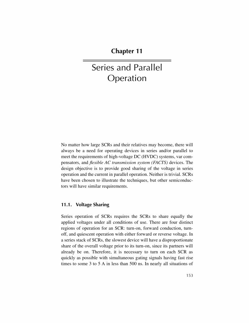
153
Chapter 11
Series and Parallel Operation
No matter how large SCRs and their relatives may become, there willalways be a need for operating devices in series and/or parallel tomeet the requirements of high-voltage DC (HVDC) systems, var com-pensators, and
flexible AC transmission system (FACTS)
devices. Thedesign objective is to provide good sharing of the voltage in seriesoperation and the current in parallel operation. Neither is trivial. SCRshave been chosen to illustrate the techniques, but other semiconduc-tors will have similar requirements.
11.1. Voltage Sharing
Series operation of SCRs requires the SCRs to share equally theapplied voltages under all conditions of use. There are four distinctregions of operation for an SCR: turn-on, forward conduction, turn-off, and quiescent operation with either forward or reverse voltage. Ina series stack of SCRs, the slowest device will have a disproportionateshare of the overall voltage prior to its turn-on, since its partners willalready be on. Therefore, it is necessary to turn on each SCR asquickly as possible with simultaneous gating signals having fast risetimes to some 3 to 5 A in less than 500 ns. In nearly all situations of
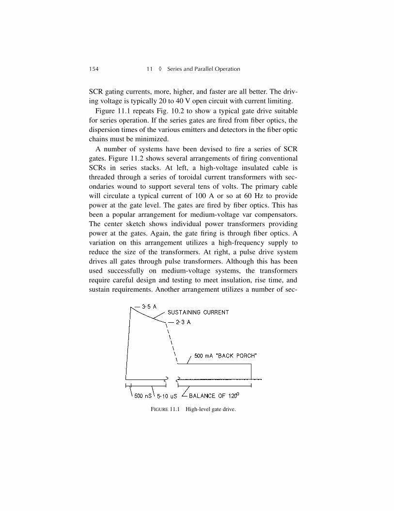
154 11
◊
Series and Parallel Operation
SCR gating currents, more, higher, and faster are all better. The driv-ing voltage is typically 20 to 40 V open circuit with current limiting.
Figure 11.1 repeats Fig. 10.2 to show a typical gate drive suitablefor series operation. If the series gates are fired from fiber optics, thedispersion times of the various emitters and detectors in the fiber opticchains must be minimized.
A number of systems have been devised to fire a series of SCRgates. Figure 11.2 shows several arrangements of firing conventionalSCRs in series stacks. At left, a high-voltage insulated cable isthreaded through a series of toroidal current transformers with sec-ondaries wound to support several tens of volts. The primary cablewill circulate a typical current of 100 A or so at 60 Hz to providepower at the gate level. The gates are fired by fiber optics. This hasbeen a popular arrangement for medium-voltage var compensators.The center sketch shows individual power transformers providingpower at the gates. Again, the gate firing is through fiber optics. Avariation on this arrangement utilizes a high-frequency supply toreduce the size of the transformers. At right, a pulse drive systemdrives all gates through pulse transformers. Although this has beenused successfully on medium-voltage systems, the transformersrequire careful design and testing to meet insulation, rise time, andsustain requirements. Another arrangement utilizes a number of sec-
FIGURE 11.1 High-level gate drive.
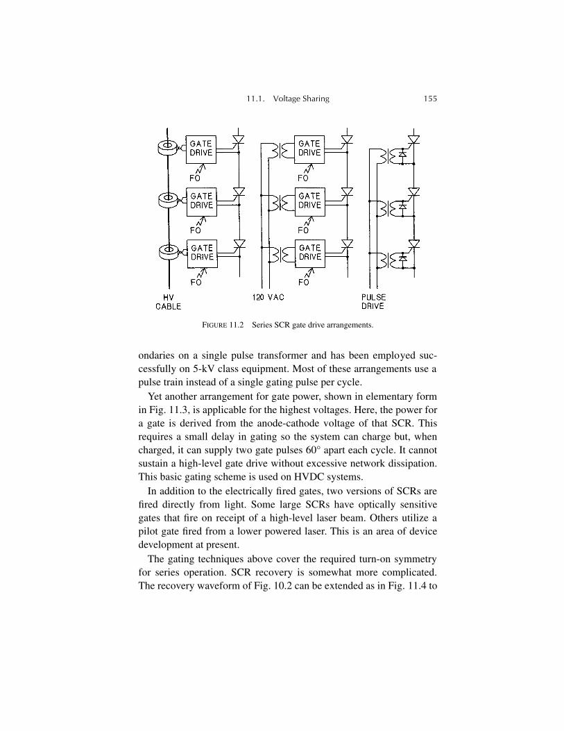
11.1. Voltage Sharing 155
ondaries on a single pulse transformer and has been employed suc-cessfully on 5-kV class equipment. Most of these arrangements use apulse train instead of a single gating pulse per cycle.
Yet another arrangement for gate power, shown in elementary formin Fig. 11.3, is applicable for the highest voltages. Here, the power fora gate is derived from the anode-cathode voltage of that SCR. Thisrequires a small delay in gating so the system can charge but, whencharged, it can supply two gate pulses 60° apart each cycle. It cannotsustain a high-level gate drive without excessive network dissipation.This basic gating scheme is used on HVDC systems.
In addition to the electrically fired gates, two versions of SCRs arefired directly from light. Some large SCRs have optically sensitivegates that fire on receipt of a high-level laser beam. Others utilize apilot gate fired from a lower powered laser. This is an area of devicedevelopment at present.
The gating techniques above cover the required turn-on symmetryfor series operation. SCR recovery is somewhat more complicated.The recovery waveform of Fig. 10.2 can be extended as in Fig. 11.4 to
FIGURE 11.2 Series SCR gate drive arrangements.
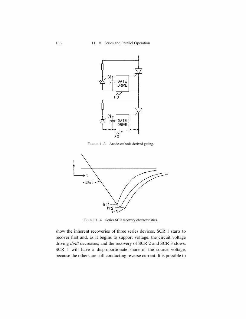
156 11
◊
Series and Parallel Operation
show the inherent recoveries of three series devices. SCR 1 starts torecover first and, as it begins to support voltage, the circuit voltagedriving
di/dt
decreases, and the recovery of SCR 2 and SCR 3 slows.SCR 1 will have a disproportionate share of the source voltage,because the others are still conducting reverse current. It is possible to
FIGURE 11.3 Anode-cathode derived gating.
FIGURE 11.4 Series SCR recovery characteristics.
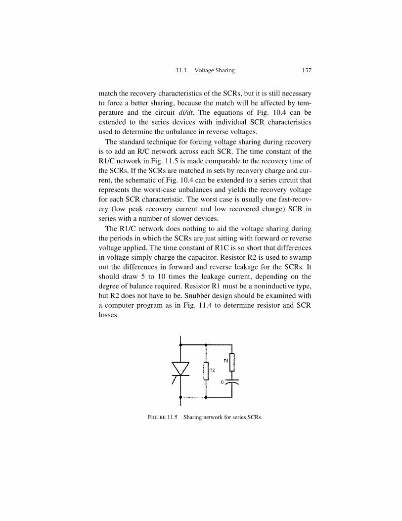
11.1. Voltage Sharing 157
match the recovery characteristics of the SCRs, but it is still necessaryto force a better sharing, because the match will be affected by tem-perature and the circuit
di/dt
. The equations of Fig. 10.4 can beextended to the series devices with individual SCR characteristicsused to determine the unbalance in reverse voltages.
The standard technique for forcing voltage sharing during recoveryis to add an R/C network across each SCR. The time constant of theR1/C network in Fig. 11.5 is made comparable to the recovery time ofthe SCRs. If the SCRs are matched in sets by recovery charge and cur-rent, the schematic of Fig. 10.4 can be extended to a series circuit thatrepresents the worst-case unbalances and yields the recovery voltagefor each SCR characteristic. The worst case is usually one fast-recov-ery (low peak recovery current and low recovered charge) SCR inseries with a number of slower devices.
The R1/C network does nothing to aid the voltage sharing duringthe periods in which the SCRs are just sitting with forward or reversevoltage applied. The time constant of R1C is so short that differencesin voltage simply charge the capacitor. Resistor R2 is used to swampout the differences in forward and reverse leakage for the SCRs. Itshould draw 5 to 10 times the leakage current, depending on thedegree of balance required. Resistor R1 must be a noninductive type,but R2 does not have to be. Snubber design should be examined witha computer program as in Fig. 11.4 to determine resistor and SCRlosses.
FIGURE 11.5 Sharing network for series SCRs.
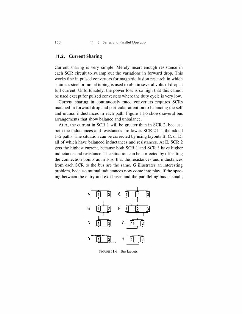
158 11
◊
Series and Parallel Operation
11.2. Current Sharing
Current sharing is very simple. Merely insert enough resistance ineach SCR circuit to swamp out the variations in forward drop. Thisworks fine in pulsed converters for magnetic fusion research in whichstainless steel or monel tubing is used to obtain several volts of drop atfull current. Unfortunately, the power loss is so high that this cannotbe used except for pulsed converters where the duty cycle is very low.
Current sharing in continuously rated converters requires SCRsmatched in forward drop and particular attention to balancing the selfand mutual inductances in each path. Figure 11.6 shows several busarrangements that show balance and unbalance.
At A, the current in SCR 1 will be greater than in SCR 2, becauseboth the inductances and resistances are lower. SCR 2 has the added1–2 paths. The situation can be corrected by using layouts B, C, or D,all of which have balanced inductances and resistances. At E, SCR 2gets the highest current, because both SCR 1 and SCR 3 have higherinductance and resistance. The situation can be corrected by offsettingthe connection points as in F so that the resistances and inductancesfrom each SCR to the bus are the same. G illustrates an interestingproblem, because mutual inductances now come into play. If the spac-ing between the entry and exit buses and the paralleling bus is small,
FIGURE 11.6 Bus layouts.
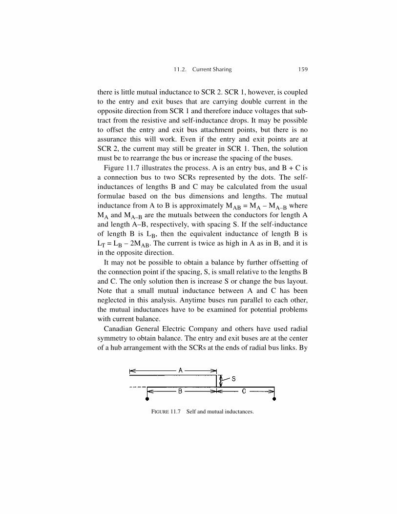
11.2. Current Sharing 159
there is little mutual inductance to SCR 2. SCR 1, however, is coupledto the entry and exit buses that are carrying double current in theopposite direction from SCR 1 and therefore induce voltages that sub-tract from the resistive and self-inductance drops. It may be possibleto offset the entry and exit bus attachment points, but there is noassurance this will work. Even if the entry and exit points are atSCR 2, the current may still be greater in SCR 1. Then, the solutionmust be to rearrange the bus or increase the spacing of the buses.
Figure 11.7 illustrates the process. A is an entry bus, and B + C isa connection bus to two SCRs represented by the dots. The self-inductances of lengths B and C may be calculated from the usualformulae based on the bus dimensions and lengths. The mutualinductance from A to B is approximately M
AB
= M
A
– M
A–B
whereM
A
and M
A–B
are the mutuals between the conductors for length Aand length A–B, respectively, with spacing S. If the self-inductanceof length B is L
B
, then the equivalent inductance of length B isL
T
= L
B
– 2M
AB
. The current is twice as high in A as in B, and it isin the opposite direction.
It may not be possible to obtain a balance by further offsetting ofthe connection point if the spacing, S, is small relative to the lengths Band C. The only solution then is increase S or change the bus layout.Note that a small mutual inductance between A and C has beenneglected in this analysis. Anytime buses run parallel to each other,the mutual inductances have to be examined for potential problemswith current balance.
Canadian General Electric Company and others have used radialsymmetry to obtain balance. The entry and exit buses are at the centerof a hub arrangement with the SCRs at the ends of radial bus links. By
FIGURE 11.7 Self and mutual inductances.
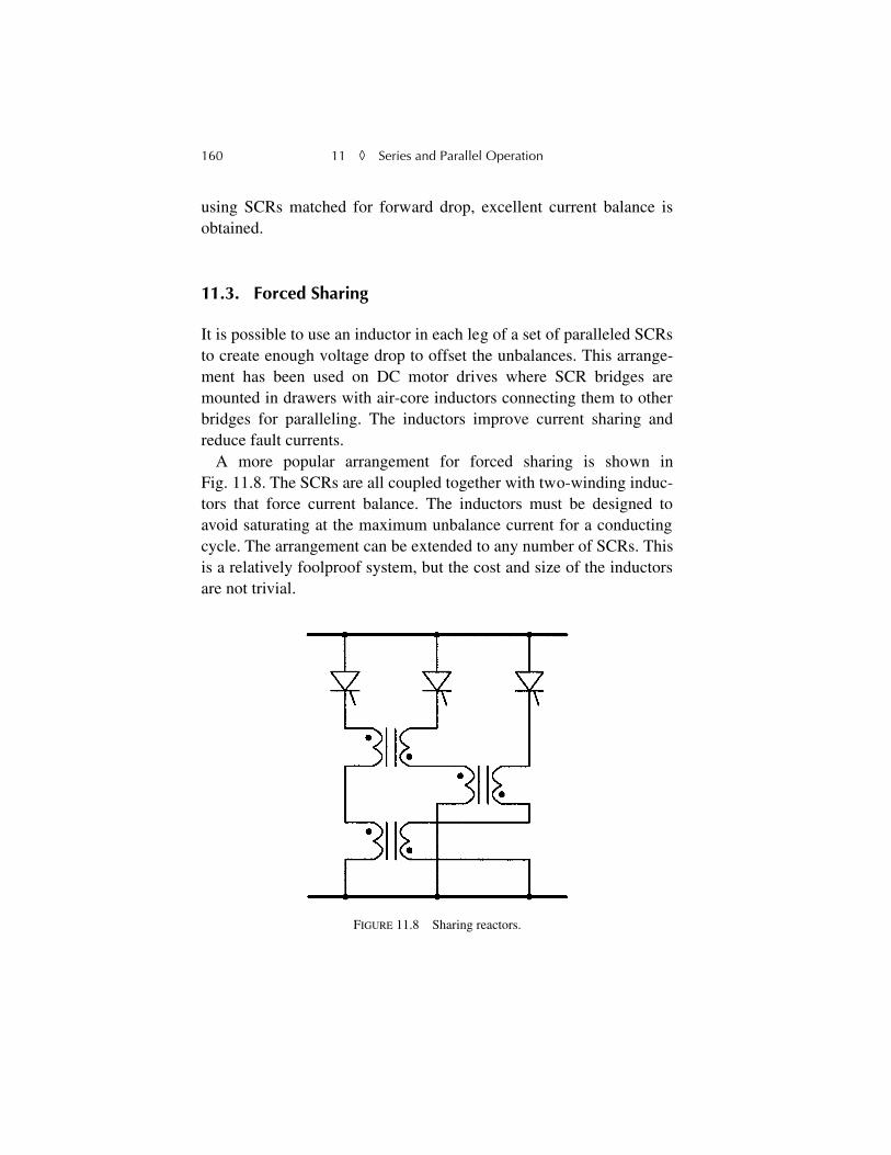
160 11
◊
Series and Parallel Operation
using SCRs matched for forward drop, excellent current balance isobtained.
11.3. Forced Sharing
It is possible to use an inductor in each leg of a set of paralleled SCRsto create enough voltage drop to offset the unbalances. This arrange-ment has been used on DC motor drives where SCR bridges aremounted in drawers with air-core inductors connecting them to otherbridges for paralleling. The inductors improve current sharing andreduce fault currents.
A more popular arrangement for forced sharing is shown inFig. 11.8. The SCRs are all coupled together with two-winding induc-tors that force current balance. The inductors must be designed toavoid saturating at the maximum unbalance current for a conductingcycle. The arrangement can be extended to any number of SCRs. Thisis a relatively foolproof system, but the cost and size of the inductorsare not trivial.
FIGURE 11.8 Sharing reactors.

11.3. Forced Sharing 161
The gate drive comments made in regard to series operation applyalso to paralleling. The first SCR to turn on will tend to steal theanode voltage necessary to turn on the rest and will have a high
di/dt
,so the process must take place as evenly as possible. A high-level,fast-rising gate pulse will assure that all SCRs turn on. Again, it is agreat kindness to the SCRs to use high-level gating in any application.

163
Chapter 12
Pulsed Converters
The SCR will probably have a long design life in applications callingfor short pulses of high currents. Its ability to latch means it cannot beforced out of a saturated condition by overload, as is the case with theinsulated gate bipolar transistors (IGBT). When used as an AC powersource, the SCR is able to supply fault currents sufficient to permitselective breaker tripping for minimum system disturbance. Thedesign of high-power pulsed converter systems is an art of its own,and some of the principles are discussed in this chapter. The authorhas had the privilege of working on a number of fascinating applica-tions in this specialized area.
12.1. Protective Devices
Most switchgear items carry a short time rating that must be respectedfor pulsed service. Protective relays may be inverse-time types to per-mit carrying high currents for a short time without tripping a breaker.Instantaneous elements must be set above the maximum current, ofcourse. A wide variety of overcurrent relay characteristics is avail-able—inverse, very inverse, and extremely inverse in both short-timeand long-time versions. Within a given type, current taps and a timedial allow adjustment over a very wide range of tripping times and
164 12
◊
Pulsed Converters
currents. For example, if an extremely inverse-time overcurrent relayis selected to trip a breaker at a given current after a very long time,the breaker will remain closed at 5 times this current for 1 sec, 10times this current for 0.3 sec, and 40 times this current for 0.1 sec witha particular setting of the time dial. Manufacturer’s data sheets pro-vide further information on overcurrent relays.
Fuses are available in a wide variety of characteristics to suitalmost any need, from slow-blow glass control fuses to high-speedsemiconductor fuses to medium-voltage fuses for motor circuits ortransformer protection. Curves are provided that show the meltingtime/current characteristic and the fault limiting level in the case ofsemiconductor-type fuses that clear subcycle. In general, fusesshould not be operated at pulsed rms currents in excess of about 60%of the melting current for the pulse time. This will assure a long life.Again, the manufacturer’s data sheets should be consulted for furtherinformation.
12.2. Transformers
Transformers generally can be operated well above their thermal rat-ings for short periods. The limiting factor may be the transient temper-ature rise although, more often, it will be a limit on electromagneticforces. Transformers can be designed with bracing of the coils so as topermit repetitive short pulses at more than 15 times the thermal rating.For example, the four transformers built for the Alcator C-MOD toka-mak at MIT were designed with cruciform cores, heavy rolled steelcylindrical core surrounds, interleaved round primary and secondarywindings, and polyester fiberglass high-strength coil wrappers. Eachtransformer was rated for 3750 kVA continuous and 58,000 kVA for apulse that rose to peak current in 2 sec, carried peak current for 1 sec,and dropped to zero in another 2 sec. The pulse repeated every 20 min.These transformers have been in service for some 20 years now andhave delivered many thousands of pulses. Similar transformers havebeen used in various ratings on tokamak supplies at Oak Ridge
12.2. Transformers 165
National Laboratories (a 300-ms pulse), General Atomic Company,and Princeton Plasma Physics Laboratory. Most are core-style drytypes.
A standard transformer can usually be operated at three to five timesrated current on a duty cycle that does not exceed the long-time kVArating. Transformers must be designed to cope with the forces gener-ated by an occasional load fault, so all have the capability to handle afew cycles of, perhaps, 20 times rated current. The catch is that, with-out special protection and bracing, the lifetime under repetitive pulsedduty may be very short. The forces vary as the square of the current,and there is no sure way to establish a pulsed rating for a standardtransformer.
A transformer specification for pulsed service must consider theresistance and leakage reactance. Pulsed converters generally operateat large commutation angles because of the inherently high operatingreactance of transformers designed for pulsed service. For example,the MIT transformers cited above were specified for a maximumleakage reactance of 0.02 pu on the thermal base, a very low-reac-tance design. On the pulse rating, however, the reactance becomes0.02
×
15 = 0.30 pu. In the absence of commutation overlap, the for-mula
Ed
=
Edo
–
Xpu
/2 defines the voltage drop from commutationloss with an inductive load,
Ed
being the output voltage at full load,
Edo
the open circuit voltage, and
Xpu
the leakage reactance on thepulse rating base. The resistance drop, in effect, subtracts directlyfrom this output voltage. If a very low reactance is specified, the costincreases because the geometry of the transformer will likely departfrom the most economical design. Low reactance requires long, thincoils and may require interlacing the windings. On the other hand, ahigh reactance drop means the no-load voltage must increase to pro-vide the needed full-load voltage. Hence, the kVA rating and cost goup. Furthermore, the commutating angle at zero phase retard and fullload is given as cos(
u
) = 1 –
Xpu
. If
Xpu
exceeds 0.134 for a 12-pulseconverter or 0.5 pu for a 6-pulse converter, the commutating angle(30° or 60°, respectively) is large enough to cause commutation over-
166 12
◊
Pulsed Converters
lap between phases and an even greater loss of voltage. Since thespecification will define the final cost and performance of the trans-former, the various design options should be discussed with the ven-dor before a specification is finalized.
12.3. SCRs
Design considerations for series and parallel operation of SCRs werediscussed in Chapter 11. All of these factors apply to SCRs in pulsedservice, but there are further considerations for this specialized classof operation, most of which are involved with the conduction lossesand junction temperatures. If the forward drop curve for the chosenSCR does not extend to the required peak current, the vendor shouldbe consulted for an extended voltage drop curve. A reasonableapproximation can usually be made by fitting a fixed voltage drop anda resistive rise with current to the published curve as far as it goes, andthen extrapolating to higher currents. With a forward drop curve inhand, the instantaneous loss can be calculated as
P
=
i(t) v(i)
and thenused in the thermal modeling described in Chapter 15. In pulsed ser-vice, the switching losses are typically not significant unless the dutycycle is high.
Operating at high pulse currents may require consideration of theturn-on
di/dt
. This has been a serious problem in the design of railguns and similar applications in which the SCRs must switch veryhigh currents. Special SCRs have been designed with highly interdig-itated gate structures so as to turn on the entire cathode area as quicklyas possible and minimize the turn-on losses. Although the full cathodearea may be able to conduct a very high current, the SCR can bedestroyed by localized heating in the cathode structure as small con-ducting areas attempt to cope with very high currents at turn-on.These gate designs are also used on fast recovery SCRs for high-fre-quency operation where switching losses become important.
Yet another consideration for pulsed service at high currents is thatlateral electromagnetic forces in SCR stacks may arise from currents

12.3. SCRs 167
in adjacent stacks or bus conductors. These may introduce a differen-tial in clamping force across the diameter of “hockey puck” SCRs. Aswith the considerations above, the vendor should always be consultedon any application that strays from the published data sheet.

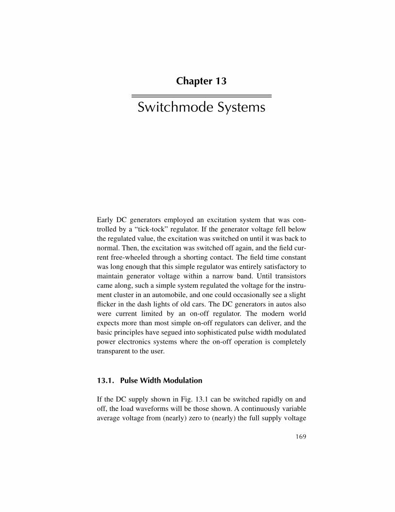
169
Chapter 13
Switchmode Systems
Early DC generators employed an excitation system that was con-trolled by a “tick-tock” regulator. If the generator voltage fell belowthe regulated value, the excitation was switched on until it was back tonormal. Then, the excitation was switched off again, and the field cur-rent free-wheeled through a shorting contact. The field time constantwas long enough that this simple regulator was entirely satisfactory tomaintain generator voltage within a narrow band. Until transistorscame along, such a simple system regulated the voltage for the instru-ment cluster in an automobile, and one could occasionally see a slightflicker in the dash lights of old cars. The DC generators in autos alsowere current limited by an on-off regulator. The modern worldexpects more than most simple on-off regulators can deliver, and thebasic principles have segued into sophisticated pulse width modulatedpower electronics systems where the on-off operation is completelytransparent to the user.
13.1. Pulse Width Modulation
If the DC supply shown in Fig. 13.1 can be switched rapidly on andoff, the load waveforms will be those shown. A continuously variableaverage voltage from (nearly) zero to (nearly) the full supply voltage
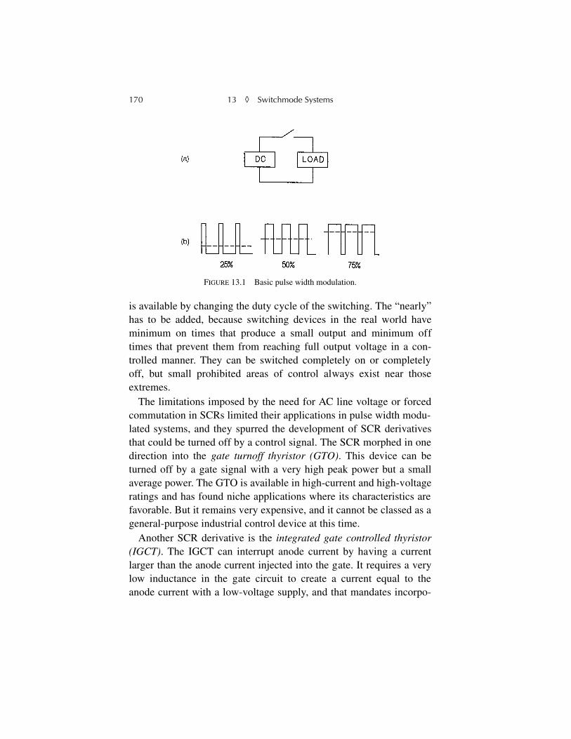
170 13
◊
Switchmode Systems
is available by changing the duty cycle of the switching. The “nearly”has to be added, because switching devices in the real world haveminimum on times that produce a small output and minimum offtimes that prevent them from reaching full output voltage in a con-trolled manner. They can be switched completely on or completelyoff, but small prohibited areas of control always exist near thoseextremes.
The limitations imposed by the need for AC line voltage or forcedcommutation in SCRs limited their applications in pulse width modu-lated systems, and they spurred the development of SCR derivativesthat could be turned off by a control signal. The SCR morphed in onedirection into the
gate turnoff thyristor (GTO)
. This device can beturned off by a gate signal with a very high peak power but a smallaverage power. The GTO is available in high-current and high-voltageratings and has found niche applications where its characteristics arefavorable. But it remains very expensive, and it cannot be classed as ageneral-purpose industrial control device at this time.
Another SCR derivative is the
integrated gate controlled thyristor(IGCT)
. The IGCT can interrupt anode current by having a currentlarger than the anode current injected into the gate. It requires a verylow inductance in the gate circuit to create a current equal to theanode current with a low-voltage supply, and that mandates incorpo-
FIGURE 13.1 Basic pulse width modulation.

13.1. Pulse Width Modulation 171
rating the gate driver into the physical packaging of the IGCT. Therequired energy storage for the gate signal is aided by the use of“supercaps,” low-voltage electrolytic capacitors with a very highenergy density. Again, the device is not really suitable for general-pur-pose use, although it has been used successfully in high-power appli-cations. Both the GTO and the IGCT are somewhat handicapped bythe regenerative, latching characteristic of the parent SCR. They donot cease conduction gracefully but must be driven out from the gate.
Developments on power transistors continued through the years andresulted in a breakthrough when a field effect transistor was weddedto a conventional bipolar transistor. The result, the
integrated gatebipolar transistor (IGBT)
, is rapidly becoming the device of choicefor many applications. It has engendered a host of new high-powerequipment designs featuring switchmode operation. The device hasthe ability to operate at frequencies several orders of magnitudehigher than the SCR, although the higher-power IGBTs are more lim-ited in their maximum frequency.
The IGBT has a PNP power transistor controlled by a field effecttransistor such that it has the best properties of each. It can handlevery high powers and yet be controlled by a gate that, being insulatedand field controlled, draws no current. Figure 13.2 shows the collec-tor-emitter voltage as a function of the collector current for severaldifferent gate-emitter voltages. As the gate voltage is increased, theIGBT begins to draw current, and this current increases with collectorvoltage until a region is reached at which the current is constant for agiven gate voltage. At high levels of gate voltage, however, a saturatedregion is reached in which the collector-emitter voltage varies onlyslightly with collector current. Although the IGBT can be operated asa linear amplifier in the same manner as a transistor, it is almostalways operated as a switch between off and on with enough gatedrive so it remains at the lowest possible voltage drop for the requiredcurrent. The saturated voltage drop is typically in the 3.0-V range.IGBTs are currently available in voltages to 6000 V and currents to2000 A. Most large IGBTs are packaged in a molded plastic assembly
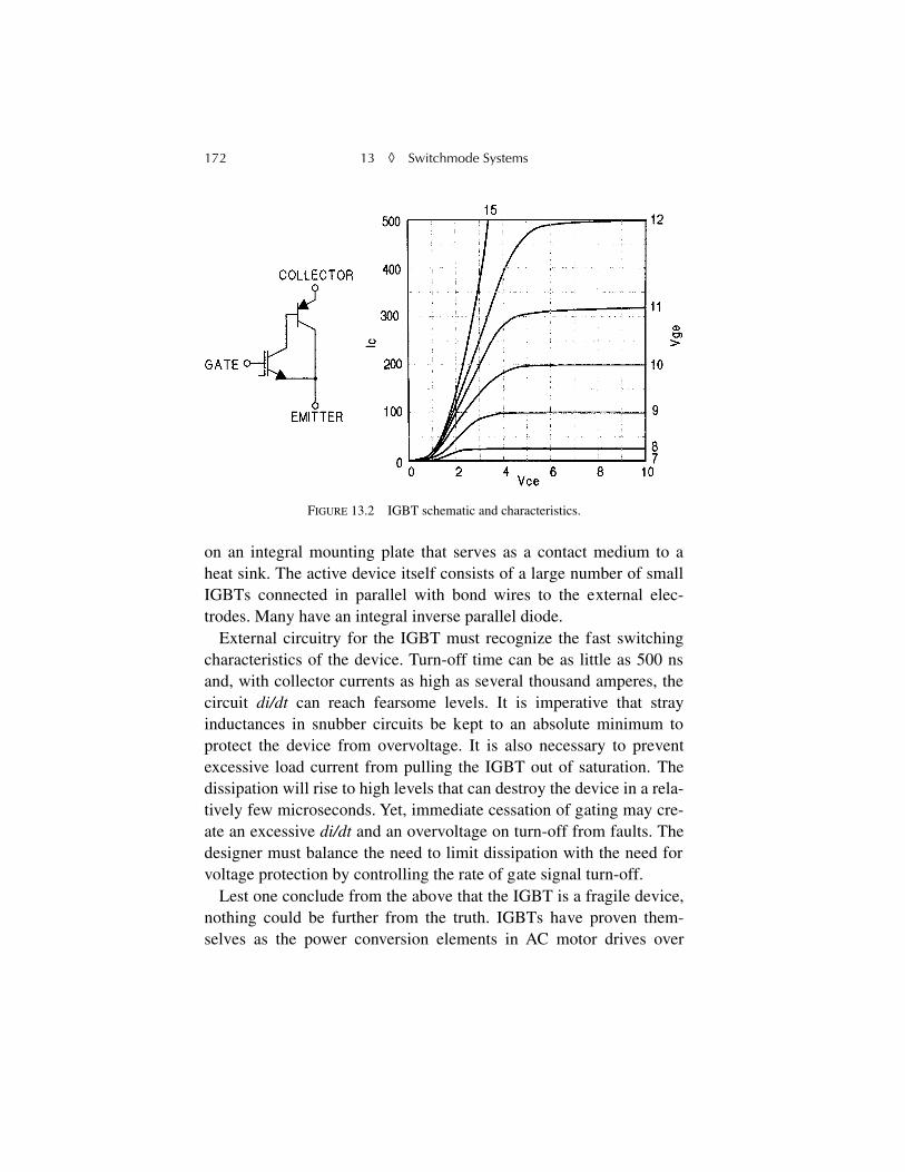
172 13
◊
Switchmode Systems
on an integral mounting plate that serves as a contact medium to aheat sink. The active device itself consists of a large number of smallIGBTs connected in parallel with bond wires to the external elec-trodes. Many have an integral inverse parallel diode.
External circuitry for the IGBT must recognize the fast switchingcharacteristics of the device. Turn-off time can be as little as 500 nsand, with collector currents as high as several thousand amperes, thecircuit
di/dt
can reach fearsome levels. It is imperative that strayinductances in snubber circuits be kept to an absolute minimum toprotect the device from overvoltage. It is also necessary to preventexcessive load current from pulling the IGBT out of saturation. Thedissipation will rise to high levels that can destroy the device in a rela-tively few microseconds. Yet, immediate cessation of gating may cre-ate an excessive
di/dt
and an overvoltage on turn-off from faults. Thedesigner must balance the need to limit dissipation with the need forvoltage protection by controlling the rate of gate signal turn-off.
Lest one conclude from the above that the IGBT is a fragile device,nothing could be further from the truth. IGBTs have proven them-selves as the power conversion elements in AC motor drives over
FIGURE 13.2 IGBT schematic and characteristics.
13.2. Choppers 173
20,000 hp and in choppers for DC electric arc furnaces at power levelsabove 100 MW. They are rugged, reliable devices.
13.2. Choppers
In Fig. 13.3, an inductor, an IGBT, and a commutating diode havebeen added to the simple switching system of Fig. 13.1 to form achopper. When the IGBT is on, the inductor and load current areincreased slightly. When it is off, load current circulates through theinductor and diode. The IGBT is always fully on or off. The ripplevoltage, exaggerated for illustration, is a function of the operating fre-quency and the inductance.
There are trade-offs between switching frequency and dissipation inthe switch. A low operating frequency leads to more ripple in the out-
FIGURE 13.3 Chopper circuit and waveforms.
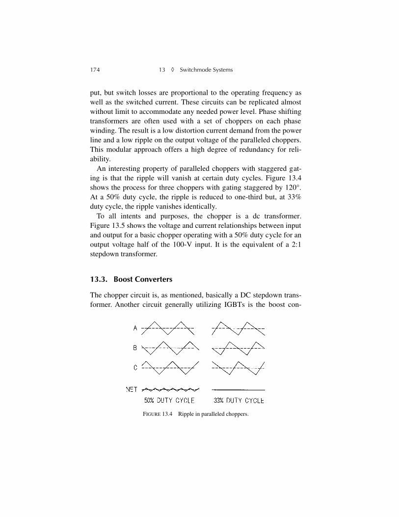
174 13
◊
Switchmode Systems
put, but switch losses are proportional to the operating frequency aswell as the switched current. These circuits can be replicated almostwithout limit to accommodate any needed power level. Phase shiftingtransformers are often used with a set of choppers on each phasewinding. The result is a low distortion current demand from the powerline and a low ripple on the output voltage of the paralleled choppers.This modular approach offers a high degree of redundancy for reli-ability.
An interesting property of paralleled choppers with staggered gat-ing is that the ripple will vanish at certain duty cycles. Figure 13.4shows the process for three choppers with gating staggered by 120°.At a 50% duty cycle, the ripple is reduced to one-third but, at 33%duty cycle, the ripple vanishes identically.
To all intents and purposes, the chopper is a dc transformer.Figure 13.5 shows the voltage and current relationships between inputand output for a basic chopper operating with a 50% duty cycle for anoutput voltage half of the 100-V input. It is the equivalent of a 2:1stepdown transformer.
13.3. Boost Converters
The chopper circuit is, as mentioned, basically a DC stepdown trans-former. Another circuit generally utilizing IGBTs is the boost con-
FIGURE 13.4 Ripple in paralleled choppers.
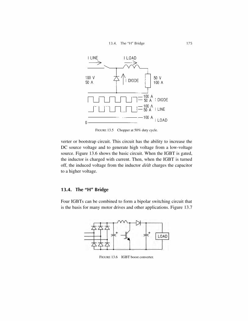
13.4. The “H” Bridge 175
verter or bootstrap circuit. This circuit has the ability to increase theDC source voltage and to generate high voltage from a low-voltagesource. Figure 13.6 shows the basic circuit. When the IGBT is gated,the inductor is charged with current. Then, when the IGBT is turnedoff, the induced voltage from the inductor
di/dt
charges the capacitorto a higher voltage.
13.4. The “H” Bridge
Four IGBTs can be combined to form a bipolar switching circuit thatis the basis for many motor drives and other applications. Figure 13.7
FIGURE 13.5 Chopper at 50% duty cycle.
FIGURE 13.6 IGBT boost converter.
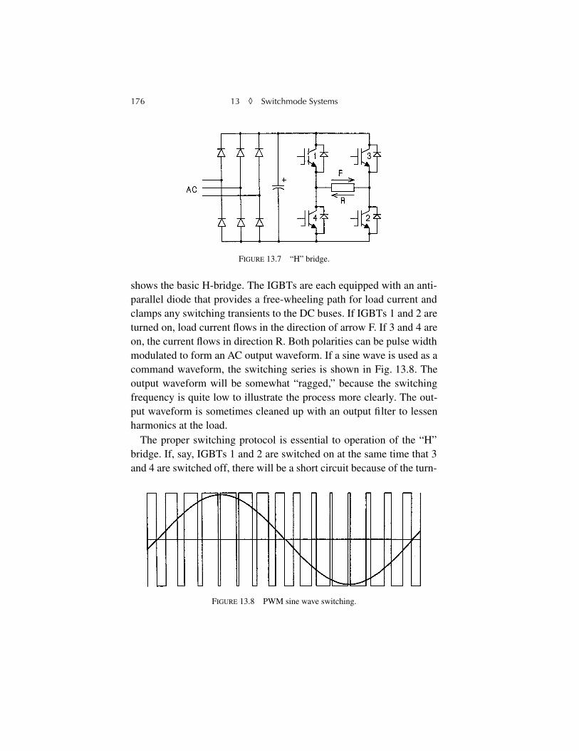
176 13
◊
Switchmode Systems
shows the basic H-bridge. The IGBTs are each equipped with an anti-parallel diode that provides a free-wheeling path for load current andclamps any switching transients to the DC buses. If IGBTs 1 and 2 areturned on, load current flows in the direction of arrow F. If 3 and 4 areon, the current flows in direction R. Both polarities can be pulse widthmodulated to form an AC output waveform. If a sine wave is used as acommand waveform, the switching series is shown in Fig. 13.8. Theoutput waveform will be somewhat “ragged,” because the switchingfrequency is quite low to illustrate the process more clearly. The out-put waveform is sometimes cleaned up with an output filter to lessenharmonics at the load.
The proper switching protocol is essential to operation of the “H”bridge. If, say, IGBTs 1 and 2 are switched on at the same time that 3and 4 are switched off, there will be a short circuit because of the turn-
FIGURE 13.7 “H” bridge.
FIGURE 13.8 PWM sine wave switching.
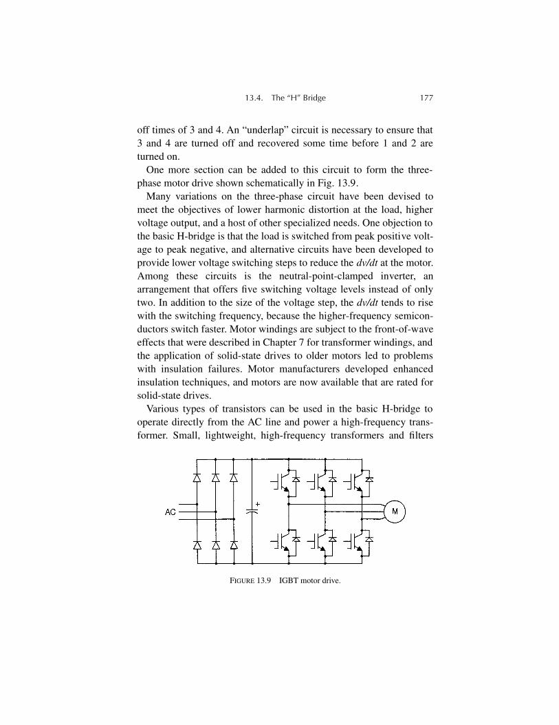
13.4. The “H” Bridge 177
off times of 3 and 4. An “underlap” circuit is necessary to ensure that3 and 4 are turned off and recovered some time before 1 and 2 areturned on.
One more section can be added to this circuit to form the three-phase motor drive shown schematically in Fig. 13.9.
Many variations on the three-phase circuit have been devised tomeet the objectives of lower harmonic distortion at the load, highervoltage output, and a host of other specialized needs. One objection tothe basic H-bridge is that the load is switched from peak positive volt-age to peak negative, and alternative circuits have been developed toprovide lower voltage switching steps to reduce the
dv/dt
at the motor.Among these circuits is the neutral-point-clamped inverter, anarrangement that offers five switching voltage levels instead of onlytwo. In addition to the size of the voltage step, the
dv/dt
tends to risewith the switching frequency, because the higher-frequency semicon-ductors switch faster. Motor windings are subject to the front-of-waveeffects that were described in Chapter 7 for transformer windings, andthe application of solid-state drives to older motors led to problemswith insulation failures. Motor manufacturers developed enhancedinsulation techniques, and motors are now available that are rated forsolid-state drives.
Various types of transistors can be used in the basic H-bridge tooperate directly from the AC line and power a high-frequency trans-former. Small, lightweight, high-frequency transformers and filters
FIGURE 13.9 IGBT motor drive.
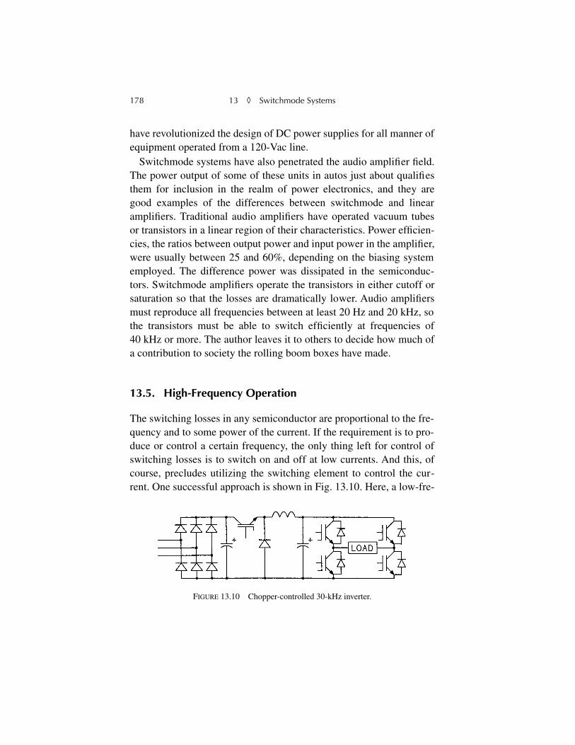
178 13
◊
Switchmode Systems
have revolutionized the design of DC power supplies for all manner ofequipment operated from a 120-Vac line.
Switchmode systems have also penetrated the audio amplifier field.The power output of some of these units in autos just about qualifiesthem for inclusion in the realm of power electronics, and they aregood examples of the differences between switchmode and linearamplifiers. Traditional audio amplifiers have operated vacuum tubesor transistors in a linear region of their characteristics. Power efficien-cies, the ratios between output power and input power in the amplifier,were usually between 25 and 60%, depending on the biasing systememployed. The difference power was dissipated in the semiconduc-tors. Switchmode amplifiers operate the transistors in either cutoff orsaturation so that the losses are dramatically lower. Audio amplifiersmust reproduce all frequencies between at least 20 Hz and 20 kHz, sothe transistors must be able to switch efficiently at frequencies of40 kHz or more. The author leaves it to others to decide how much ofa contribution to society the rolling boom boxes have made.
13.5. High-Frequency Operation
The switching losses in any semiconductor are proportional to the fre-quency and to some power of the current. If the requirement is to pro-duce or control a certain frequency, the only thing left for control ofswitching losses is to switch on and off at low currents. And this, ofcourse, precludes utilizing the switching element to control the cur-rent. One successful approach is shown in Fig. 13.10. Here, a low-fre-
FIGURE 13.10 Chopper-controlled 30-kHz inverter.
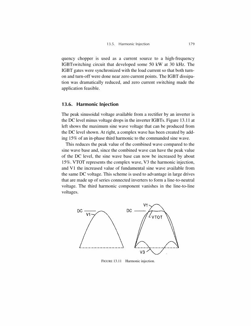
13.5. Harmonic Injection 179
quency chopper is used as a current source to a high-frequencyIGBTswitching circuit that developed some 50 kW at 30 kHz. TheIGBT gates were synchronized with the load current so that both turn-on and turn-off were done near zero current points. The IGBT dissipa-tion was dramatically reduced, and zero current switching made theapplication feasible.
13.6. Harmonic Injection
The peak sinusoidal voltage available from a rectifier by an inverter isthe DC level minus voltage drops in the inverter IGBTs. Figure 13.11 atleft shows the maximum sine wave voltage that can be produced fromthe DC level shown. At right, a complex wave has been created by add-ing 15% of an in-phase third harmonic to the commanded sine wave.
This reduces the peak value of the combined wave compared to thesine wave base and, since the combined wave can have the peak valueof the DC level, the sine wave base can now be increased by about15%. VTOT represents the complex wave, V3 the harmonic injection,and V1 the increased value of fundamental sine wave available fromthe same DC voltage. This scheme is used to advantage in large drivesthat are made up of series connected inverters to form a line-to-neutralvoltage. The third harmonic component vanishes in the line-to-linevoltages.
FIGURE 13.11 Harmonic injection.
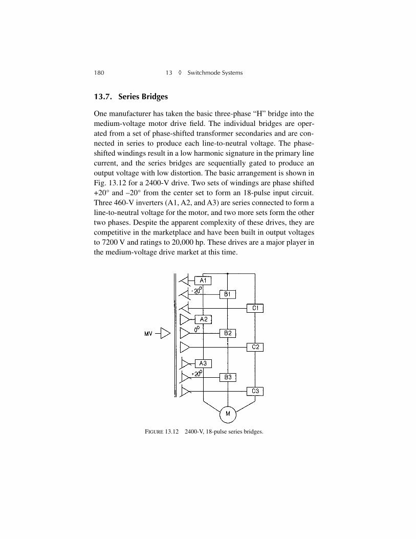
180 13
◊
Switchmode Systems
13.7. Series Bridges
One manufacturer has taken the basic three-phase “H” bridge into themedium-voltage motor drive field. The individual bridges are oper-ated from a set of phase-shifted transformer secondaries and are con-nected in series to produce each line-to-neutral voltage. The phase-shifted windings result in a low harmonic signature in the primary linecurrent, and the series bridges are sequentially gated to produce anoutput voltage with low distortion. The basic arrangement is shown inFig. 13.12 for a 2400-V drive. Two sets of windings are phase shifted+20° and –20° from the center set to form an 18-pulse input circuit.Three 460-V inverters (A1, A2, and A3) are series connected to form aline-to-neutral voltage for the motor, and two more sets form the othertwo phases. Despite the apparent complexity of these drives, they arecompetitive in the marketplace and have been built in output voltagesto 7200 V and ratings to 20,000 hp. These drives are a major player inthe medium-voltage drive market at this time.
FIGURE 13.12 2400-V, 18-pulse series bridges.

181
Chapter 14
Power Factor and Harmonics
It may seem odd to treat these two quantities together, but power fac-tor correction in the presence of harmonic currents poses special prob-lems, and correction of harmonic problems may affect the circuitpower factor. The two are best considered together so their interac-tions can be better understood. The author had the pleasure of present-ing tutorial sessions on power factor and harmonics for several yearsat national meetings of the IEEE Industry Applications Society.
14.1. Power Factor
Power factor, as everyone knows, is defined as the ratio of real powerto volt-amperes and is the cosine of the phase angle between the volt-age and current in an AC circuit. These are neatly defined quantitieswith sinusoidal voltages and currents. Power factor can be improvedby adding capacitors on the power line to draw a leading current andsupply lagging vars to the system. Power factor correction capacitorscan be switched in and out as necessary to maintain var and voltagecontrol.
As mentioned in Chapter 1, many utilities charge industrial custom-ers a certain rate for kilowatt-hours of energy consumed in a month,and another charge related to the infrastructure necessary to supply
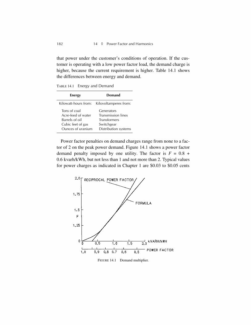
182 14
◊
Power Factor and Harmonics
that power under the customer’s conditions of operation. If the cus-tomer is operating with a low power factor load, the demand charge ishigher, because the current requirement is higher. Table 14.1 showsthe differences between energy and demand.
Power factor penalties on demand charges range from none to a fac-tor of 2 on the peak power demand. Figure 14.1 shows a power factordemand penalty imposed by one utility. The factor is
F
= 0.8 +0.6
kvarh/kWh, but not less than 1 and not more than 2. Typical valuesfor power charges as indicated in Chapter 1 are $0.03 to $0.05 cents
T
ABLE
14.1
Energy and Demand
Energy Demand
Kilowatt-hours from: Kilovoltamperes from:
Tons of coalAcre-feed of waterBarrels of oilCubic feet of gasOunces of uranium
GeneratorsTransmission linesTransformersSwitchgearDistribution systems
FIGURE 14.1 Demand multiplier.
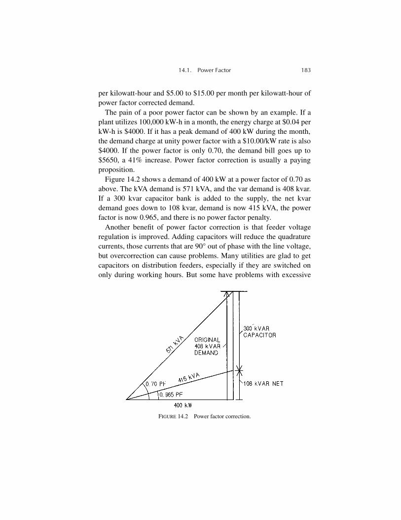
14.1. Power Factor 183
per kilowatt-hour and $5.00 to $15.00 per month per kilowatt-hour ofpower factor corrected demand.
The pain of a poor power factor can be shown by an example. If aplant utilizes 100,000 kW-h in a month, the energy charge at $0.04 perkW-h is $4000. If it has a peak demand of 400 kW during the month,the demand charge at unity power factor with a $10.00/kW rate is also$4000. If the power factor is only 0.70, the demand bill goes up to$5650, a 41% increase. Power factor correction is usually a payingproposition.
Figure 14.2 shows a demand of 400 kW at a power factor of 0.70 asabove. The kVA demand is 571 kVA, and the var demand is 408 kvar.If a 300 kvar capacitor bank is added to the supply, the net kvardemand goes down to 108 kvar, demand is now 415 kVA, the powerfactor is now 0.965, and there is no power factor penalty.
Another benefit of power factor correction is that feeder voltageregulation is improved. Adding capacitors will reduce the quadraturecurrents, those currents that are 90° out of phase with the line voltage,but overcorrection can cause problems. Many utilities are glad to getcapacitors on distribution feeders, especially if they are switched ononly during working hours. But some have problems with excessive
FIGURE 14.2 Power factor correction.
184 14
◊
Power Factor and Harmonics
voltage rise during periods of light load, and some may have tariffsthat discriminate against leading power factors, too. The same kVAcapacity is required for a given leading load power factor as for a lag-ging one.
Some plant engineers have a pathological fear of a leading powerfactor for reasons the author could never fathom. In point of fact, noload has any idea what the power factor is and couldn’t care less. Ithas been scientifically proven that leading power factors do not causeillness to machines or humans. The only possible concern for a lead-ing power factor is overvoltage at light load if the power factor goestoo far leading.
In a large plant, power factor correction can be applied at the inter-face between the utility and the customer, the point of
common cou-pling,
as it is termed. This is generally less expensive than adding a lotof small capacitor banks, particularly when switchgear is required orharmonics are present.
14.2. Harmonics
Harmonics are familiar to the musician as the overtones from aninstrument. They are the integer multiples of the instrument’s funda-mental or natural frequency that are produced by a series of standingwaves of higher and higher order. The precise mathematical descrip-tion of this phenomenon creates the equal tempered chromatic scalethat is reproduced in Table 14.2.
Exactly the same thing happens in power circuits when nonsinusoi-dal loads create harmonic currents that are integer multiples of thesupply frequency. The rapid growth of solid-state power electronicshas greatly increased the number and size of these loads, and the restof this chapter is devoted to examining their origin, their interactionswith the utility, and their control.
A number of nonsinusoidal waveforms were shown in Chapter 6 inconjunction with phase control circuits. The basic mechanism bywhich harmonics produce nonsinusoidal waveforms is shown in
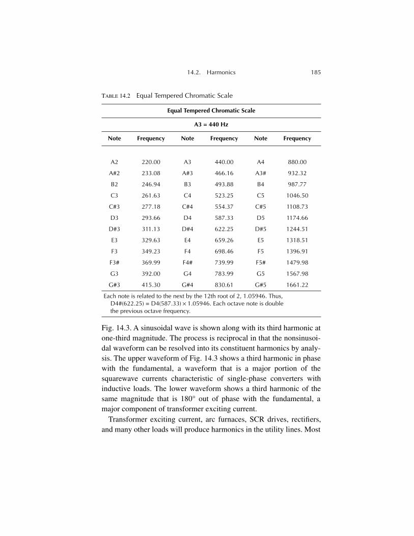
14.2. Harmonics 185
Fig. 14.3. A sinusoidal wave is shown along with its third harmonic atone-third magnitude. The process is reciprocal in that the nonsinusoi-dal waveform can be resolved into its constituent harmonics by analy-sis. The upper waveform of Fig. 14.3 shows a third harmonic in phasewith the fundamental, a waveform that is a major portion of thesquarewave currents characteristic of single-phase converters withinductive loads. The lower waveform shows a third harmonic of thesame magnitude that is 180° out of phase with the fundamental, amajor component of transformer exciting current.
Transformer exciting current, arc furnaces, SCR drives, rectifiers,and many other loads will produce harmonics in the utility lines. Most
T
ABLE
14.2
Equal Tempered Chromatic Scale
Equal Tempered Chromatic Scale
A3 = 440 Hz
Note Frequency Note Frequency Note Frequency
A2 220.00 A3 440.00 A4 880.00
A#2 233.08 A#3 466.16 A3# 932.32
B2 246.94 B3 493.88 B4 987.77
C3 261.63 C4 523.25 C5 1046.50
C#3 277.18 C#4 554.37 C#5 1108.73
D3 293.66 D4 587.33 D5 1174.66
D#3 311.13 D#4 622.25 D#5 1244.51
E3 329.63 E4 659.26 E5 1318.51
F3 349.23 F4 698.46 F5 1396.91
F3# 369.99 F4# 739.99 F5# 1479.98
G3 392.00 G4 783.99 G5 1567.98
G#3 415.30 G#4 830.61 G#5 1661.22
Each note is related to the next by the 12th root of 2, 1.05946. Thus, D4#(622.25) = D4(587.33)
×
1.05946. Each octave note is double the previous octave frequency.
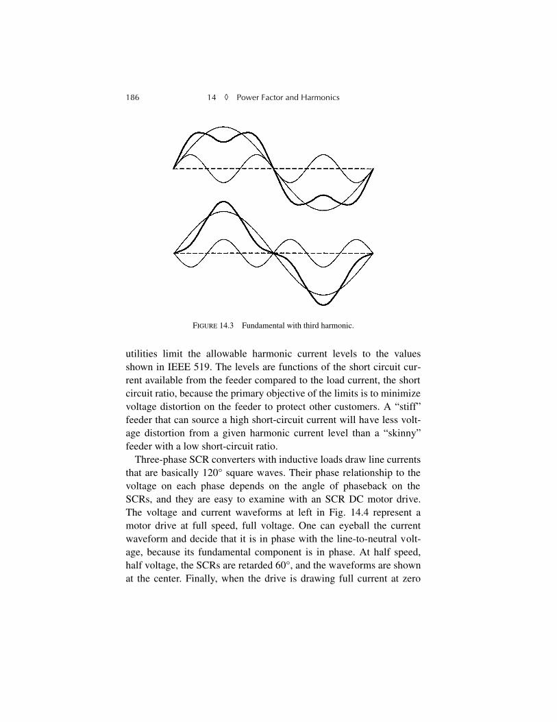
186 14
◊
Power Factor and Harmonics
utilities limit the allowable harmonic current levels to the valuesshown in IEEE 519. The levels are functions of the short circuit cur-rent available from the feeder compared to the load current, the shortcircuit ratio, because the primary objective of the limits is to minimizevoltage distortion on the feeder to protect other customers. A “stiff”feeder that can source a high short-circuit current will have less volt-age distortion from a given harmonic current level than a “skinny”feeder with a low short-circuit ratio.
Three-phase SCR converters with inductive loads draw line currentsthat are basically 120° square waves. Their phase relationship to thevoltage on each phase depends on the angle of phaseback on theSCRs, and they are easy to examine with an SCR DC motor drive.The voltage and current waveforms at left in Fig. 14.4 represent amotor drive at full speed, full voltage. One can eyeball the currentwaveform and decide that it is in phase with the line-to-neutral volt-age, because its fundamental component is in phase. At half speed,half voltage, the SCRs are retarded 60°, and the waveforms are shownat the center. Finally, when the drive is drawing full current at zero
FIGURE 14.3 Fundamental with third harmonic.
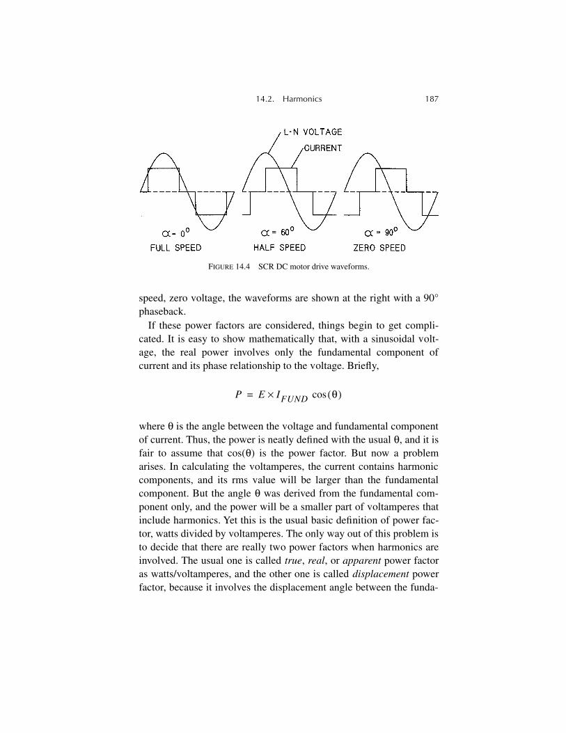
14.2. Harmonics 187
speed, zero voltage, the waveforms are shown at the right with a 90°phaseback.
If these power factors are considered, things begin to get compli-cated. It is easy to show mathematically that, with a sinusoidal volt-age, the real power involves only the fundamental component ofcurrent and its phase relationship to the voltage. Briefly,
where
θ
is the angle between the voltage and fundamental componentof current. Thus, the power is neatly defined with the usual
θ
, and it isfair to assume that cos(
θ
) is the power factor. But now a problemarises. In calculating the voltamperes, the current contains harmoniccomponents, and its rms value will be larger than the fundamentalcomponent. But the angle
θ
was derived from the fundamental com-ponent only, and the power will be a smaller part of voltamperes thatinclude harmonics. Yet this is the usual basic definition of power fac-tor, watts divided by voltamperes. The only way out of this problem isto decide that there are really two power factors when harmonics areinvolved. The usual one is called
true
,
real
, or
apparent
power factoras watts/voltamperes, and the other one is called
displacement
powerfactor, because it involves the displacement angle between the funda-
FIGURE 14.4 SCR DC motor drive waveforms.
P E IFUND θ( )cos×=
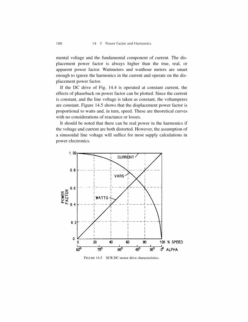
188 14
◊
Power Factor and Harmonics
mental voltage and the fundamental component of current. The dis-placement power factor is always higher than the true, real, orapparent power factor. Wattmeters and watthour meters are smartenough to ignore the harmonics in the current and operate on the dis-placement power factor.
If the DC drive of Fig. 14.4 is operated at constant current, theeffects of phaseback on power factor can be plotted. Since the currentis constant, and the line voltage is taken as constant, the voltamperesare constant. Figure 14.5 shows that the displacement power factor isproportional to watts and, in turn, speed. These are theoretical curveswith no considerations of reactance or losses.
It should be noted that there can be real power in the harmonics ifthe voltage and current are both distorted. However, the assumption ofa sinusoidal line voltage will suffice for most supply calculations inpower electronics.
FIGURE 14.5 SCR DC motor drive characteristics.
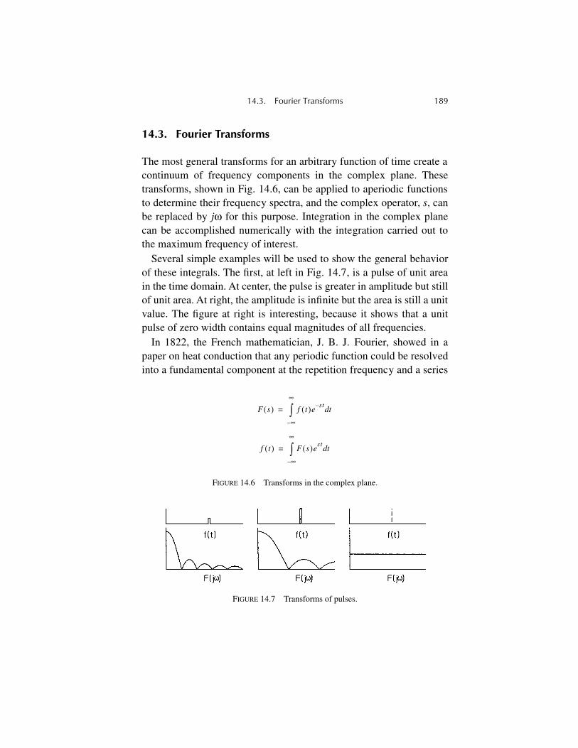
14.3. Fourier Transforms 189
14.3. Fourier Transforms
The most general transforms for an arbitrary function of time create acontinuum of frequency components in the complex plane. Thesetransforms, shown in Fig. 14.6, can be applied to aperiodic functionsto determine their frequency spectra, and the complex operator,
s
, canbe replaced by
j
ω
for this purpose. Integration in the complex planecan be accomplished numerically with the integration carried out tothe maximum frequency of interest.
Several simple examples will be used to show the general behaviorof these integrals. The first, at left in Fig. 14.7, is a pulse of unit areain the time domain. At center, the pulse is greater in amplitude but stillof unit area. At right, the amplitude is infinite but the area is still a unitvalue. The figure at right is interesting, because it shows that a unitpulse of zero width contains equal magnitudes of all frequencies.
In 1822, the French mathematician, J. B. J. Fourier, showed in apaper on heat conduction that any periodic function could be resolvedinto a fundamental component at the repetition frequency and a series
F s( ) f t( )est–
td
∞–
∞
∫=
f t( ) F s( )est
td
∞–
∞
∫=
FIGURE 14.6 Transforms in the complex plane.
FIGURE 14.7 Transforms of pulses.
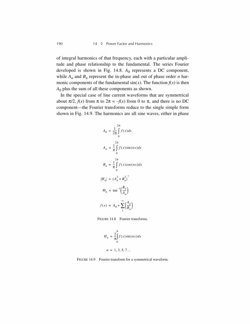
190 14
◊
Power Factor and Harmonics
of integral harmonics of that frequency, each with a particular ampli-tude and phase relationship to the fundamental. The series Fourierdeveloped is shown in Fig. 14.8.
A
0
represents a DC component,while
A
n
and
B
n
represent the in-phase and out of phase order
n
har-monic components of the fundamental sin(
x
). The function
f
(
x
) is then
A
0
plus the sum of all these components as shown.In the special case of line current waveforms that are symmetrical
about
π
/2,
f
(
x
) from
π
to 2
π
= –
f
(
x
) from 0 to
π
, and there is no DCcomponent—the Fourier transforms reduce to the single simple formshown in Fig. 14.9. The harmonics are all sine waves, either in phase
A01
2π------ f x( ) xd
0
2π
∫=
An1π--- f x( ) nx( )sin xd
0
2π
∫=
Bn1π--- f x( ) nx( )cos xd
0
2π
∫=
Hn An2
Bn2
+( )?
=
Θn tan1– Bn
An------⎝ ⎠
⎛ ⎞=
f x( ) A0
An
Bn------⎝ ⎠
⎛ ⎞
1
∞
∑+=
FIGURE 14.8 Fourier transforms.
FIGURE 14.9 Fourier transform for a symmetrical waveform.
Hn2π--- f x( ) nx( )sin xd
0
π
∫=
n 1 3 5 7…, , ,=
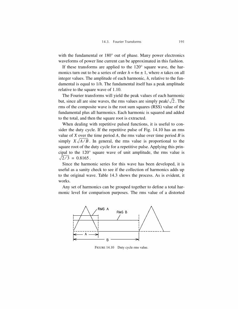
14.3. Fourier Transforms 191
with the fundamental or 180° out of phase. Many power electronicswaveforms of power line current can be approximated in this fashion.
If these transforms are applied to the 120° square wave, the har-monics turn out to be a series of order h = 6n ± 1, where n takes on allinteger values. The amplitude of each harmonic, h, relative to the fun-damental is equal to 1/h. The fundamental itself has a peak amplituderelative to the square wave of 1.10.
The Fourier transforms will yield the peak values of each harmonicbut, since all are sine waves, the rms values are simply peak/ . Therms of the composite wave is the root sum squares (RSS) value of thefundamental plus all harmonics. Each harmonic is squared and addedto the total, and then the square root is extracted.
When dealing with repetitive pulsed functions, it is useful to con-sider the duty cycle. If the repetitive pulse of Fig. 14.10 has an rmsvalue of X over the time period A, the rms value over time period B issimply . In general, the rms value is proportional to thesquare root of the duty cycle for a repetitive pulse. Applying this prin-cipal to the 120° square wave of unit amplitude, the rms value is
.Since the harmonic series for this wave has been developed, it is
useful as a sanity check to see if the collection of harmonics adds upto the original wave. Table 14.3 shows the process. As is evident, itworks.
Any set of harmonics can be grouped together to define a total har-monic level for comparison purposes. The rms value of a distorted
2
FIGURE 14.10 Duty cycle rms value.
X A B⁄
2 3⁄ 0.8165=
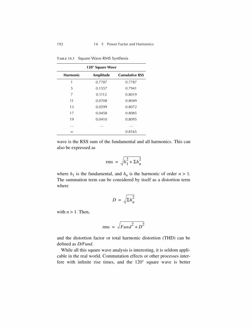
192 14 ◊ Power Factor and Harmonics
wave is the RSS sum of the fundamental and all harmonics. This canalso be expressed as
where h1 is the fundamental, and hn is the harmonic of order n > 1.The summation term can be considered by itself as a distortion termwhere
with n > 1. Then,
and the distortion factor or total harmonic distortion (THD) can bedefined as D/Fund.
While all this square wave analysis is interesting, it is seldom appli-cable in the real world. Commutation effects or other processes inter-fere with infinite rise times, and the 120° square wave is better
TABLE 14.3 Square Wave RMS Synthesis
120° Square Wave
Harmonic Amplitude Cumulative RSS
1 0.7787 0.7787
5 0.1557 0.7941
7 0.1112 0.8019
11 0.0708 0.8049
13 0.0599 0.8072
17 0.0458 0.8085
19 0.0410 0.8095
… … …
∞ 0.8165
rms h12 Σhn
2+=
D Σhn2
=
rms Fund2
D2
+=
14.3. Fourier Transforms 193
represented as a trapezoidal wave or, in the case of a converter, a1-cos(θ) rise and a cos(θ) fall where 0 ≤ θ ≤ u. The increase in thesquare wave rise and fall times “softens” the harmonic series so thatthe envelope slope of the peak higher order harmonics drops off as
instead of the 1/h at low frequencies. These represent slopes of–2 and –1, respectively when the envelopes are plotted on log-logpaper. For typical system reactances, the change in slope occurssomewhere between the 11th and 35th harmonic, the transition fre-quency being lower as the system reactance and load current increase.The practical effect of this is that the higher harmonics are somewhatless of a problem than one might expect.
While increasing reactance will reduce the higher frequencies, it isnot usually a feasible approach to harmonic mitigation. Increasingpulse numbers from phase shifting was discussed in Chapter 7 inregard to transformer connections, and this is generally the preferredmethod of reducing harmonics. If an SCR converter or a rectifier issupplied from delta and wye transformer windings and the rectifiedoutputs are connected in series or parallel, the result is 12-pulse rectifi-cation. The basic harmonic series is now h = 12n ± 1 instead of 6n ± 1.The major 5th and 7th harmonic currents are greatly reduced, as are thehigher-order ones. Still higher pulse numbers are entirely feasible, and48-pulse systems are used on large electrochemical supplies. Sincelarge rectifiers and converters require sets of paralleled SCRs ordiodes, the additional expense of the phase shifting is primarily a mat-ter of transformer cost. Figure 10.11 illustrates the advantages of a 12-pulse system as compared to a 6-pulse one. Noncharacteristic 12-pulseharmonics are shown at approximately 10% residual level, a typicalvalue. Still higher pulse numbers have characteristic harmonics ororder h = pn ± 1, where p is the pulse number.
As a note of interest, a pair of harmonics sets that are simply dis-placed 30° from each other do not cancel out the sixth-order values. Itis the travel of these harmonic currents back through the supply trans-former and thereby acquiring another phase shift that makes the can-cellation possible.
1 h2⁄
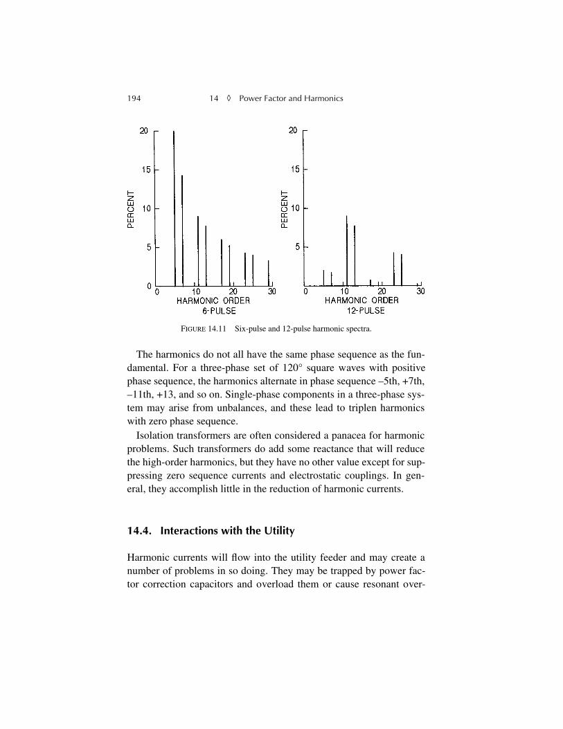
194 14 ◊ Power Factor and Harmonics
The harmonics do not all have the same phase sequence as the fun-damental. For a three-phase set of 120° square waves with positivephase sequence, the harmonics alternate in phase sequence –5th, +7th,–11th, +13, and so on. Single-phase components in a three-phase sys-tem may arise from unbalances, and these lead to triplen harmonicswith zero phase sequence.
Isolation transformers are often considered a panacea for harmonicproblems. Such transformers do add some reactance that will reducethe high-order harmonics, but they have no other value except for sup-pressing zero sequence currents and electrostatic couplings. In gen-eral, they accomplish little in the reduction of harmonic currents.
14.4. Interactions with the Utility
Harmonic currents will flow into the utility feeder and may create anumber of problems in so doing. They may be trapped by power fac-tor correction capacitors and overload them or cause resonant over-
FIGURE 14.11 Six-pulse and 12-pulse harmonic spectra.
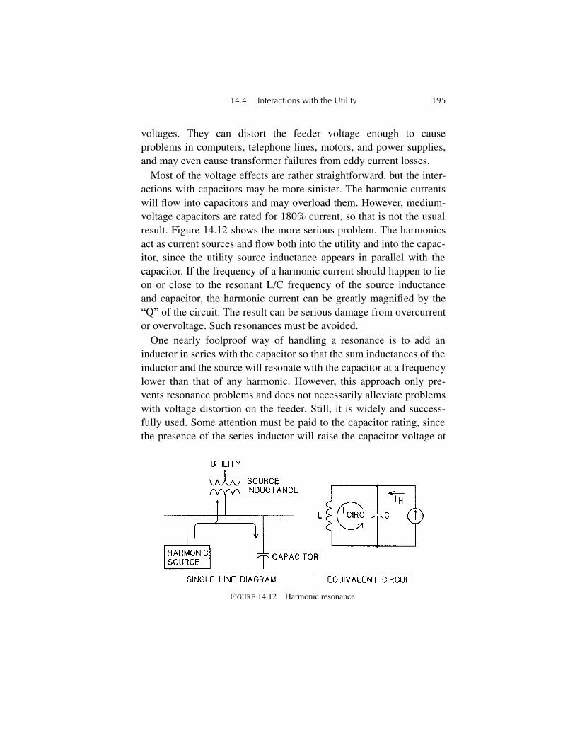
14.4. Interactions with the Utility 195
voltages. They can distort the feeder voltage enough to causeproblems in computers, telephone lines, motors, and power supplies,and may even cause transformer failures from eddy current losses.
Most of the voltage effects are rather straightforward, but the inter-actions with capacitors may be more sinister. The harmonic currentswill flow into capacitors and may overload them. However, medium-voltage capacitors are rated for 180% current, so that is not the usualresult. Figure 14.12 shows the more serious problem. The harmonicsact as current sources and flow both into the utility and into the capac-itor, since the utility source inductance appears in parallel with thecapacitor. If the frequency of a harmonic current should happen to lieon or close to the resonant L/C frequency of the source inductanceand capacitor, the harmonic current can be greatly magnified by the“Q” of the circuit. The result can be serious damage from overcurrentor overvoltage. Such resonances must be avoided.
One nearly foolproof way of handling a resonance is to add aninductor in series with the capacitor so that the sum inductances of theinductor and the source will resonate with the capacitor at a frequencylower than that of any harmonic. However, this approach only pre-vents resonance problems and does not necessarily alleviate problemswith voltage distortion on the feeder. Still, it is widely and success-fully used. Some attention must be paid to the capacitor rating, sincethe presence of the series inductor will raise the capacitor voltage at
FIGURE 14.12 Harmonic resonance.
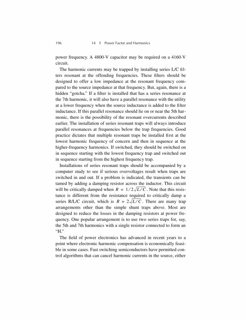
196 14 ◊ Power Factor and Harmonics
power frequency. A 4800-V capacitor may be required on a 4160-Vcircuit.
The harmonic currents may be trapped by installing series L/C fil-ters resonant at the offending frequencies. These filters should bedesigned to offer a low impedance at the resonant frequency com-pared to the source impedance at that frequency. But, again, there is ahidden “gotcha.” If a filter is installed that has a series resonance atthe 7th harmonic, it will also have a parallel resonance with the utilityat a lower frequency when the source inductance is added to the filterinductance. If this parallel resonance should lie on or near the 5th har-monic, there is the possibility of the resonant overcurrents describedearlier. The installation of series resonant traps will always introduceparallel resonances at frequencies below the trap frequencies. Goodpractice dictates that multiple resonant traps be installed first at thelowest harmonic frequency of concern and then in sequence at thehigher-frequency harmonics. If switched, they should be switched onin sequence starting with the lowest frequency trap and switched outin sequence starting from the highest frequency trap.
Installations of series resonant traps should be accompanied by acomputer study to see if serious overvoltages result when traps areswitched in and out. If a problem is indicated, the transients can betamed by adding a damping resistor across the inductor. This circuitwill be critically damped when . Note that this resis-tance is different from the resistance required to critically damp aseries R/L/C circuit, which is . There are many traparrangements other than the simple shunt traps above. Most aredesigned to reduce the losses in the damping resistors at power fre-quency. One popular arrangement is to use two series traps for, say,the 5th and 7th harmonics with a single resistor connected to form an“H.”
The field of power electronics has advanced in recent years to apoint where electronic harmonic compensation is economically feasi-ble in some cases. Fast switching semiconductors have permitted con-trol algorithms that can cancel harmonic currents in the source, either
R 1 2⁄ L C⁄=
R 2 L C⁄=
14.4. Interactions with the Utility 197
by controlling the conversion system itself or by injecting complexcurrent waveforms to cancel the distortion. Stand-alone systems areeconomically practical, at this date, for injection currents of severalhundred amperes at 600-V class, and the trend is to higher voltagesand currents.
Figure 14.13 shows the effect of filter traps on a 120° square wavecurrent with a 10° commutation angle. As the filters are added toremove the harmonics, the waveform becomes less distorted and morenearly sinusoidal. The total harmonic distortion drops from 26 to 6%as the four filters are added.
FIGURE 14.13 Harmonic trap results.
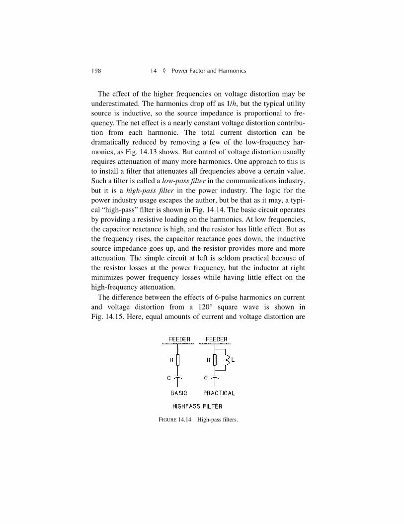
198 14 ◊ Power Factor and Harmonics
The effect of the higher frequencies on voltage distortion may beunderestimated. The harmonics drop off as 1/h, but the typical utilitysource is inductive, so the source impedance is proportional to fre-quency. The net effect is a nearly constant voltage distortion contribu-tion from each harmonic. The total current distortion can bedramatically reduced by removing a few of the low-frequency har-monics, as Fig. 14.13 shows. But control of voltage distortion usuallyrequires attenuation of many more harmonics. One approach to this isto install a filter that attenuates all frequencies above a certain value.Such a filter is called a low-pass filter in the communications industry,but it is a high-pass filter in the power industry. The logic for thepower industry usage escapes the author, but be that as it may, a typi-cal “high-pass” filter is shown in Fig. 14.14. The basic circuit operatesby providing a resistive loading on the harmonics. At low frequencies,the capacitor reactance is high, and the resistor has little effect. But asthe frequency rises, the capacitor reactance goes down, the inductivesource impedance goes up, and the resistor provides more and moreattenuation. The simple circuit at left is seldom practical because ofthe resistor losses at the power frequency, but the inductor at rightminimizes power frequency losses while having little effect on thehigh-frequency attenuation.
The difference between the effects of 6-pulse harmonics on currentand voltage distortion from a 120° square wave is shown inFig. 14.15. Here, equal amounts of current and voltage distortion are
FIGURE 14.14 High-pass filters.
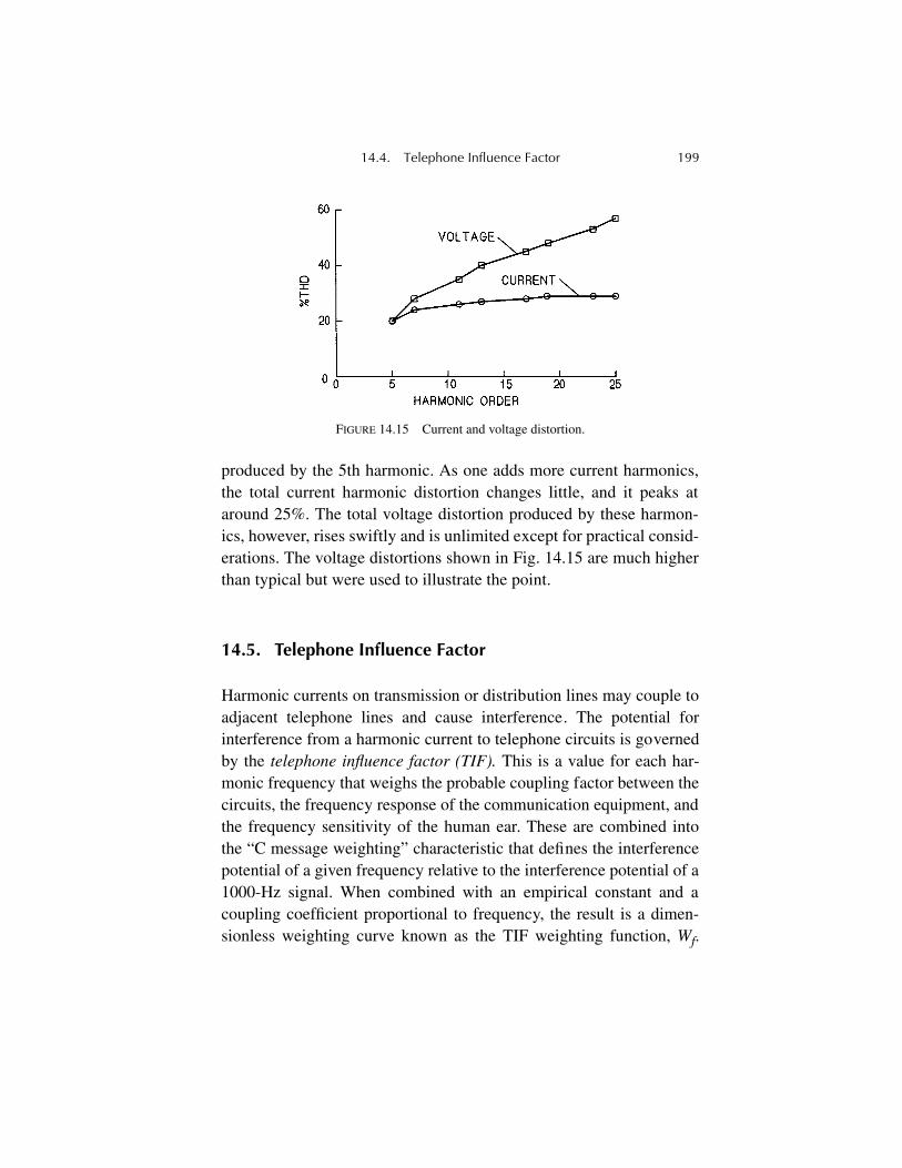
14.4. Telephone Influence Factor 199
produced by the 5th harmonic. As one adds more current harmonics,the total current harmonic distortion changes little, and it peaks ataround 25%. The total voltage distortion produced by these harmon-ics, however, rises swiftly and is unlimited except for practical consid-erations. The voltage distortions shown in Fig. 14.15 are much higherthan typical but were used to illustrate the point.
14.5. Telephone Influence Factor
Harmonic currents on transmission or distribution lines may couple toadjacent telephone lines and cause interference. The potential forinterference from a harmonic current to telephone circuits is governedby the telephone influence factor (TIF). This is a value for each har-monic frequency that weighs the probable coupling factor between thecircuits, the frequency response of the communication equipment, andthe frequency sensitivity of the human ear. These are combined intothe “C message weighting” characteristic that defines the interferencepotential of a given frequency relative to the interference potential of a1000-Hz signal. When combined with an empirical constant and acoupling coefficient proportional to frequency, the result is a dimen-sionless weighting curve known as the TIF weighting function, Wf.
FIGURE 14.15 Current and voltage distortion.
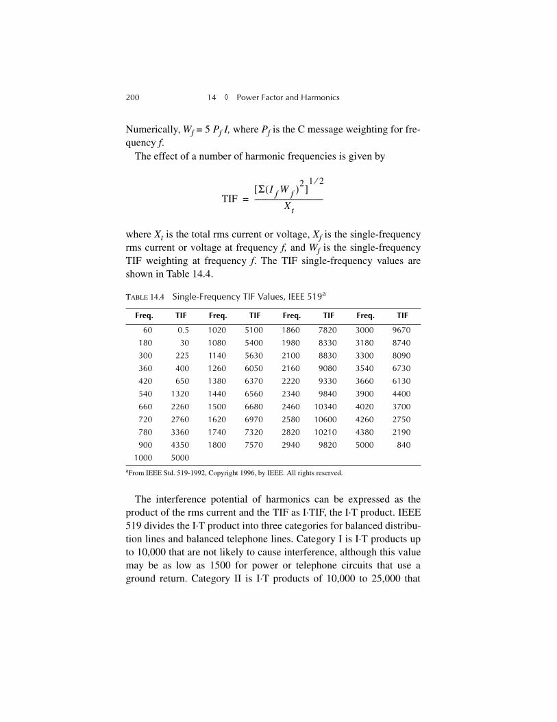
200 14 ◊ Power Factor and Harmonics
Numerically, Wf = 5 Pf I, where Pf is the C message weighting for fre-quency f.
The effect of a number of harmonic frequencies is given by
where Xt is the total rms current or voltage, Xf is the single-frequencyrms current or voltage at frequency f, and Wf is the single-frequencyTIF weighting at frequency f. The TIF single-frequency values areshown in Table 14.4.
The interference potential of harmonics can be expressed as theproduct of the rms current and the TIF as I·TIF, the I·T product. IEEE519 divides the I·T product into three categories for balanced distribu-tion lines and balanced telephone lines. Category I is I·T products upto 10,000 that are not likely to cause interference, although this valuemay be as low as 1500 for power or telephone circuits that use aground return. Category II is I·T products of 10,000 to 25,000 that
TABLE 14.4 Single-Frequency TIF Values, IEEE 519a
aFrom IEEE Std. 519-1992, Copyright 1996, by IEEE. All rights reserved.
Freq. TIF Freq. TIF Freq. TIF Freq. TIF
60 0.5 1020 5100 1860 7820 3000 9670
180 30 1080 5400 1980 8330 3180 8740
300 225 1140 5630 2100 8830 3300 8090
360 400 1260 6050 2160 9080 3540 6730
420 650 1380 6370 2220 9330 3660 6130
540 1320 1440 6560 2340 9840 3900 4400
660 2260 1500 6680 2460 10340 4020 3700
720 2760 1620 6970 2580 10600 4260 2750
780 3360 1740 7320 2820 10210 4380 2190
900 4350 1800 7570 2940 9820 5000 840
1000 5000
TIFΣ I f W f( )2[ ]
1 2⁄
Xt---------------------------------------=
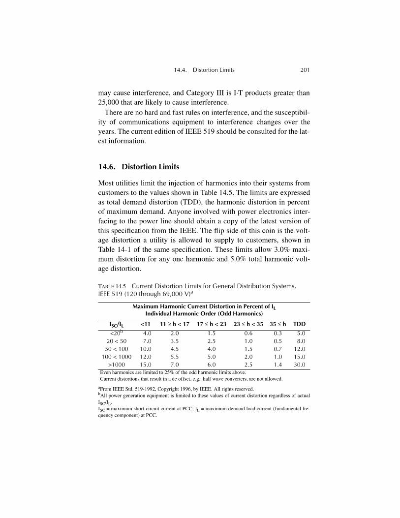
14.4. Distortion Limits 201
may cause interference, and Category III is I·T products greater than25,000 that are likely to cause interference.
There are no hard and fast rules on interference, and the susceptibil-ity of communications equipment to interference changes over theyears. The current edition of IEEE 519 should be consulted for the lat-est information.
14.6. Distortion Limits
Most utilities limit the injection of harmonics into their systems fromcustomers to the values shown in Table 14.5. The limits are expressedas total demand distortion (TDD), the harmonic distortion in percentof maximum demand. Anyone involved with power electronics inter-facing to the power line should obtain a copy of the latest version ofthis specification from the IEEE. The flip side of this coin is the volt-age distortion a utility is allowed to supply to customers, shown inTable 14-1 of the same specification. These limits allow 3.0% maxi-mum distortion for any one harmonic and 5.0% total harmonic volt-age distortion.
TABLE 14.5 Current Distortion Limits for General Distribution Systems, IEEE 519 (120 through 69,000 V)a
aFrom IEEE Std. 519-1992, Copyright 1996, by IEEE. All rights reserved.
Maximum Harmonic Current Distortion in Percent of ILIndividual Harmonic Order (Odd Harmonics)
ISC/IL <11 11 ≥ h < 17 17 ≤ h < 23 23 ≤ h < 35 35 ≤ h TDD
<20b
bAll power generation equipment is limited to these values of current distortion regardless of actualISC/IL.ISC = maximum short-circuit current at PCC; IL = maximum demand load current (fundamental fre-quency component) at PCC.
4.0 2.0 1.5 0.6 0.3 5.020 < 50 7.0 3.5 2.5 1.0 0.5 8.050 < 100 10.0 4.5 4.0 1.5 0.7 12.0
100 < 1000 12.0 5.5 5.0 2.0 1.0 15.0>1000 15.0 7.0 6.0 2.5 1.4 30.0
Even harmonics are limited to 25% of the odd harmonic limits above.Current distortions that result in a dc offset, e.g., half wave converters, are not allowed.
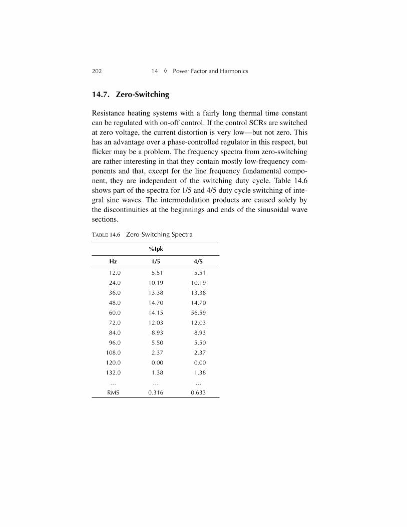
202 14 ◊ Power Factor and Harmonics
14.7. Zero-Switching
Resistance heating systems with a fairly long thermal time constantcan be regulated with on-off control. If the control SCRs are switchedat zero voltage, the current distortion is very low—but not zero. Thishas an advantage over a phase-controlled regulator in this respect, butflicker may be a problem. The frequency spectra from zero-switchingare rather interesting in that they contain mostly low-frequency com-ponents and that, except for the line frequency fundamental compo-nent, they are independent of the switching duty cycle. Table 14.6shows part of the spectra for 1/5 and 4/5 duty cycle switching of inte-gral sine waves. The intermodulation products are caused solely bythe discontinuities at the beginnings and ends of the sinusoidal wavesections.
TABLE 14.6 Zero-Switching Spectra
%Ipk
Hz 1/5 4/5
12.0 5.51 5.51
24.0 10.19 10.19
36.0 13.38 13.38
48.0 14.70 14.70
60.0 14.15 56.59
72.0 12.03 12.03
84.0 8.93 8.93
96.0 5.50 5.50
108.0 2.37 2.37
120.0 0.00 0.00
132.0 1.38 1.38
… … …
RMS 0.316 0.633
203
Chapter 15
Thermal Considerations
Many years ago, the author was involved in the design of a small tran-sistor inverter for an early space application. The interesting problemwith this unit was that, in the vacuum of space, there is no convectionor conduction cooling. All heat must be removed by radiation.Accordingly, the aluminum case was milled with rounded ridges topresent the largest possible surface area and radiation normal to thesurface at all angles. Since that time, there has been a succession of airand water cooled systems, but that was the only one that relied solelyon radiation for cooling.
15.1. Heat and Heat Transfer
Some thermal relationships may help put cooling systems in perspec-tive. Table 15.1 covers some of the basics.
Enclosure cooling is by convection and radiation. The several for-mulae involved can be simplified for rule-of-thumb estimates of heatloss as follows:
Radiation
W
= 0.00235
Tr
1.19
η....
Tr
= (426 ·
W
/
η
)
0.84
204 15
◊
Thermal Considerations
Convection (natural)
W
= 0.0014
Tr
1.25
Tr
= (714 ·
W
)
0.80
where
W
= watts per square inch
Tr
= temperature rise in degrees Celsius
η
= the emissivity
These two formulas are useful from 0 to 50°C, and both are approxi-mations developed by the author.
The effective radiating surface of a painted object is approximatelythe area of a sheet stretched around the maximum dimensions. Theconvecting area of an object is the sum of the areas of sides, ends, andtop surfaces. The side areas are not applicable to an enclosure lineupexcept for the end units. Emissivity of common materials is shown inTable 15.2. As the table shows, paint color matters only for aesthetics.
T
ABLE
15.1
Thermal Constants
• Specific heat is the ratio of the thermal capacity of a material to that of the same weight of water at 15°C.
∆
T
=
Q/ms
where
Q
is the applied heat,
m
is the mass, and
s
is the specific heat.
• Thermal conductivity is the time rate of heat transfer by conduction through a unit thickness, across a unit area for a unit difference of temperature.
∆
T
=
Qd/ka
where
Q
is the applied heat,
d
is the material thickness,
k
is the thermal con-ductivity, and
a
is the area.
• One calorie will raise the temperature of 1 g of water 1°C in 1 sec. One calorie is equivalent to 4.18 Joule. One Joule equals 1 W-sec.
• A heat input of 1000 cal/sec will raise the temperature of a water flow of 1 L/sec by 1°C. A heat input of 1 kW will raise a water flow of 1 gpm by 3.8°C.
Properties of various materials
MaterialSpecific gravity,
g/ccSpecific heat,
cal/g
Thermalconductivity,
cal-g/cm
2
/s/°C
Water 1.00 1.00 1.00
Steel 7.70 0.12 0.11
Aluminum 2.70 0.21 0.50
Copper 8.90 0.09 0.92
15.2. Air Cooling 205
15.2. Air Cooling
Air-cooled heat sink assemblies in the higher power ratings usuallyrequire forced airflow. This may take the form of high-velocity fanson the heat sinks or an overall ventilation system, and the two areoften combined. It is good practice to equip the heat sinks with ther-mal switches to detect loss of sufficient airflow. Heat sink fans shouldbe mounted close to the heat sink and, ideally, fans and heat sinksshrouded to confine the airflow. Overall enclosure airflow can be pro-vided by ceiling mounted exhaust fans or by a master air handlingsystem involving a series of enclosures. The latter usually requires acentrifugal fan to provide the necessary pressure, because ducting incabinets produces relatively high head losses.
Air velocity across heat sinks can be measured by the exhaust air-flow with an anemometer. Some anemometers are propeller driven,and others utilize a calibrated thermistor that is cooled by the airflow.
T
ABLE
15.2
Radiation Emissivities of Common Materials
Material Emissivity
Silver, highly polished 0.02
Aluminum, highly polished 0.05
Copper 0.15
Cast iron 0.25
Aluminum paint 0.55
Brass, polished 0.60
Oxidized steel 0.70
Black gloss paint 0.90
White lacquer 0.95
White enamel 0.95
Green paint 0.95
Lampblack 0.95
206 15
◊
Thermal Considerations
In either case, the average exhaust velocity can be determined byaveraging the indicated flows across the heat sink cross section.
Ventilating fans for heat sinks should be chosen carefully. Somefans have blade designs that provide a high airflow capacity at lowstatic head but drop off rapidly with increased head. Other types havea blade design with lesser delivery at low heads but can maintain agood delivery with high head loss. Heat sinks with a multiplicity ofclosely spaced fins are very efficient, but they have a high head lossand require a suitable fan to deliver the necessary air velocity acrossthe fins. Figure 15.1 shows two typical delivery curves.
15.3. Water Cooling
Water cooling of transformers, semiconductors, and buses yieldshigher outputs for a given size and weight of the equipment. It usuallyallows more bang for the buck. Unlike air cooling systems, watercooling requires a secondary heat exchange to another coolingmedium. Raw water is seldom suitable for electronic equipment
FIGURE 15.1 Fan delivery curves.
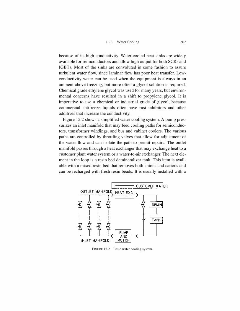
15.3. Water Cooling 207
because of its high conductivity. Water-cooled heat sinks are widelyavailable for semiconductors and allow high output for both SCRs andIGBTs. Most of the sinks are convoluted in some fashion to assureturbulent water flow, since laminar flow has poor heat transfer. Low-conductivity water can be used when the equipment is always in anambient above freezing, but more often a glycol solution is required.Chemical grade ethylene glycol was used for many years, but environ-mental concerns have resulted in a shift to propylene glycol. It isimperative to use a chemical or industrial grade of glycol, becausecommercial antifreeze liquids often have rust inhibitors and otheradditives that increase the conductivity.
Figure 15.2 shows a simplified water cooling system. A pump pres-surizes an inlet manifold that may feed cooling paths for semiconduc-tors, transformer windings, and bus and cabinet coolers. The variouspaths are controlled by throttling valves that allow for adjustment ofthe water flow and can isolate the path to permit repairs. The outletmanifold passes through a heat exchanger that may exchange heat to acustomer plant water system or a water-to-air exchanger. The next ele-ment in the loop is a resin bed demineralizer tank. This item is avail-able with a mixed resin bed that removes both anions and cations andcan be recharged with fresh resin beads. It is usually installed with a
FIGURE 15.2 Basic water cooling system.
208 15
◊
Thermal Considerations
bypass valve so that only a portion of the system flow goes throughthe tank. The tank is required, because the system (even if charged ini-tially with distilled water) will gradually acquire ions from the metalcomponents of the system and will increase in conductivity to unac-ceptable levels. Finally, the system has a filling tank that allows thesystem to be recharged and assures a positive head on the pump toprevent cavitation. It is installed at the highest point in the water sys-tem. Typically, the water loss is small enough so the makeup can betap water.
The entire system is stainless steel, plastic, or copper. Hoses are low-conductivity rubber “pot line” hose made for the electrochemicalindustry. These hoses are rated for a resistance of not less than 1 M
Ω
/ftand are pressure tested at 300 psi. Connections are secured with hoseclamps over barbed fittings. Typical accessories for a water systemwould include thermal switches, flow meters and switches, tempera-ture regulators, bypass valves, thermometers, pressure gages, remotemetering, level indicators, and vents. Pumps are usually centrifugaltypes with bronze or stainless steel impellers. Motors may run to sev-eral horsepower on larger systems. They are almost always installedas a redundant pair.
Other cooling systems for electrochemical installations have beensuccessfully made using aluminum components and heat sinks withplastic tubing and low-pressure water circulation. As with mostdesigns, there is a comfort factor associated with experience in thevarious companies building water-cooled equipment.
15.4. Device Cooling
An important area of semiconductor application involves the thermalmanagement of the junction temperature. This is a rather straightfor-ward process for steady-state operation, since the allowable currentsare well covered in the data sheet. Thermal characteristics are usuallydefined by a transient thermal impedance (TTZ) that represents thejunction temperature rise above the case temperature for a unit step
15.4. Device Cooling 209
input of power dissipation at the junction for a given time. The mount-ing interface drop and the heat sink characteristics can simply beadded to the steady-state junction-to-case thermal impedance of thedevice to obtain a composite thermal representation. The dissipationcan then be multiplied by this impedance to obtain the junction tem-perature rise above ambient.
Operation of the semiconductor in applications where the current isan odd waveform or a series of unequal current pulses is considerablymore difficult. The device TTZ from the data sheet defines the junc-tion rise above the case temperature only for a steady, continuedpower function of the indicated duration and only when the device ismounted on an infinite heat sink with no interface temperature gradi-ent. There is no simple analytical way to meld the device TTZ withthe interface drop and the heat sink TTZ. One way out of this dilemmais to represent the TTZ curve with an electrical network to whichother elements in the heat path can be concatenated.
Oliver Heaviside, in the mid-nineteenth century, showed that linearheat flow by conduction can be represented as a distributed R/C net-work of series R and shunt C. If a constant heat input is applied at oneend of an infinitely long network, the temperature at that end will risein proportion to the square root of time. In sharp contrast to the con-ventional L/C transmission line, there is no velocity of propagation inan R/C line, nor are there reflections. A current input at one endresults in an immediate output at the other end, however greatly atten-uated. The late W. E. Newell of the (then) Westinghouse ResearchLaboratories analyzed the characteristics of various electrical net-works in a series of invited papers for the IEEE, wherein he showedthat transient heat flow from a semiconductor junction could be repre-sented by a series of asymptotic responses of R/C elements. Then, forany complex input power waveform, the time response could be eval-uated by breaking the power waveform into a series of finite impulses,finding the time response for each, and then adding the results. Thisrequires the use of the convolution integral and still begs the questionof how to represent additional thermal elements of buses and heat
210 15
◊
Thermal Considerations
sinks. The author, faced with the need to evaluate asymmetric coolingof large, “hockey puck” SCRs with complex current waveforms, madethe jump to representing the entire cooling path from junction to airby means of a series of concatenated R/C elements. The approach isvalid for other semiconductors as well.
The heat transfer from a semiconductor junction to the case is byconduction, although internal material interfaces prevent it from beingpure linear diffusion. For most SCRs with brazed interfaces, the TTZcurve rises at a rate somewhat lower than
t
1/2
. Still, a series of R/Celements can be chosen to represent the curve with minimal error. Aminimum number of one element plus one element per decade of timeon the TTZ curve is suggested with a capacitor at the junction end anda final resistor. The chosen network should match the TTZ curvedown to the shortest time of interest. If the minimum applied pulse is100 ms long, there is little point in worrying about the junctionresponse at 10 µs, although recovery energy may require this consid-eration as a separate matter. The sum of the resistors must equal thesteady-state TTZ, but the capacitors must be selected by trial anderror, tapered in increasing capacitance away from the junction. Thegoodness of fit can be determined by shorting the end away from thejunction and applying a step current source of 1 A to the junction end.The voltage at the junction end should then match the TTZ curve.
An additional constraint is that the open-circuit characteristicshould depart from the short-circuit characteristic as the slope of theTTZ curve approaches the region of maximum change of curvature.The network that satisfies these two conditions should be a reasonableapproximation to the TTZ characteristic under both open- and short-circuit conditions. The interface drop can be added as a resistor to thenetwork output resistor. A heat sink TTZ characteristic can be treatedin similar fashion, although a single R/C section may suffice with aninput capacitor and a shunt resistor equal to the steady-state TTZ.These several networks can then simply be concatenated for an over-all TTZ network. Then, any arbitrary power dissipation function canbe input as a current at the junction end to develop a transient junction
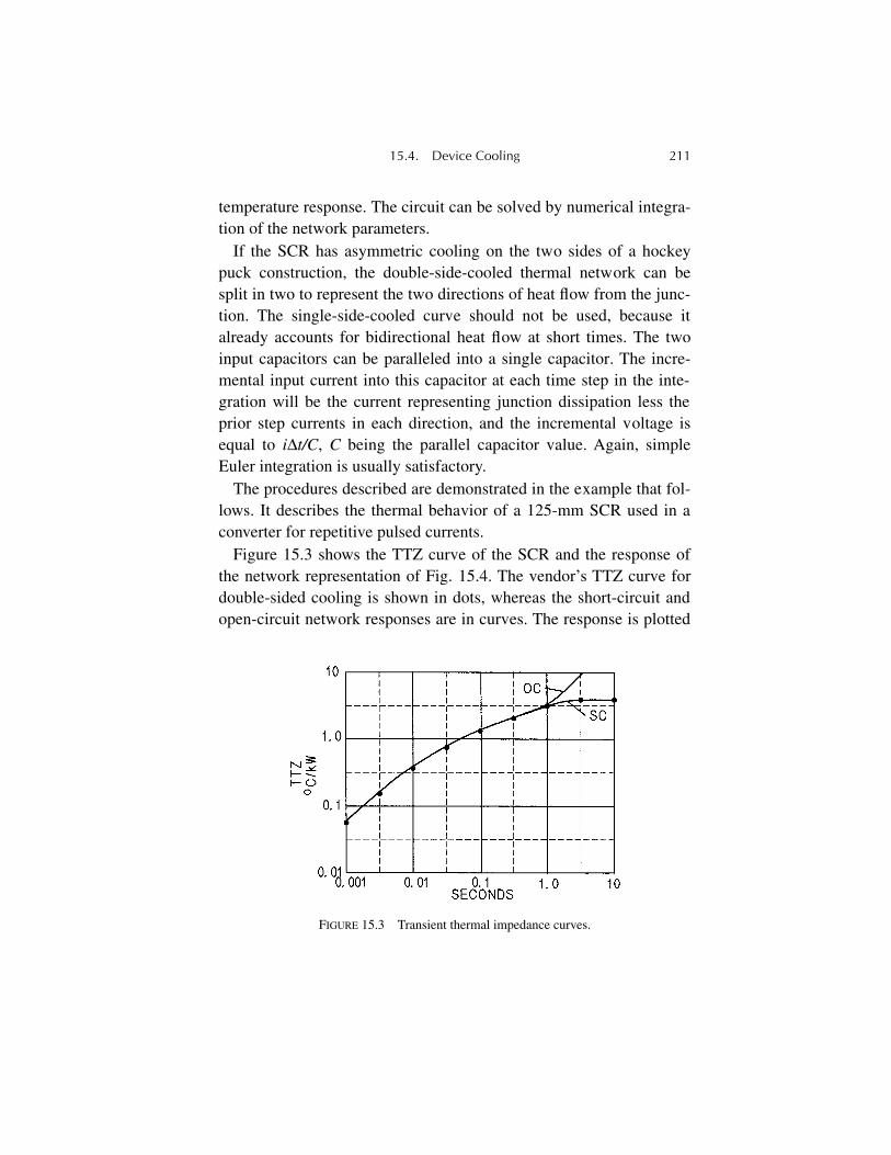
15.4. Device Cooling 211
temperature response. The circuit can be solved by numerical integra-tion of the network parameters.
If the SCR has asymmetric cooling on the two sides of a hockeypuck construction, the double-side-cooled thermal network can besplit in two to represent the two directions of heat flow from the junc-tion. The single-side-cooled curve should not be used, because italready accounts for bidirectional heat flow at short times. The twoinput capacitors can be paralleled into a single capacitor. The incre-mental input current into this capacitor at each time step in the inte-gration will be the current representing junction dissipation less theprior step currents in each direction, and the incremental voltage isequal to
i
∆
t/C
,
C
being the parallel capacitor value. Again, simpleEuler integration is usually satisfactory.
The procedures described are demonstrated in the example that fol-lows. It describes the thermal behavior of a 125-mm SCR used in aconverter for repetitive pulsed currents.
Figure 15.3 shows the TTZ curve of the SCR and the response ofthe network representation of Fig. 15.4. The vendor’s TTZ curve fordouble-sided cooling is shown in dots, whereas the short-circuit andopen-circuit network responses are in curves. The response is plotted
FIGURE 15.3 Transient thermal impedance curves.
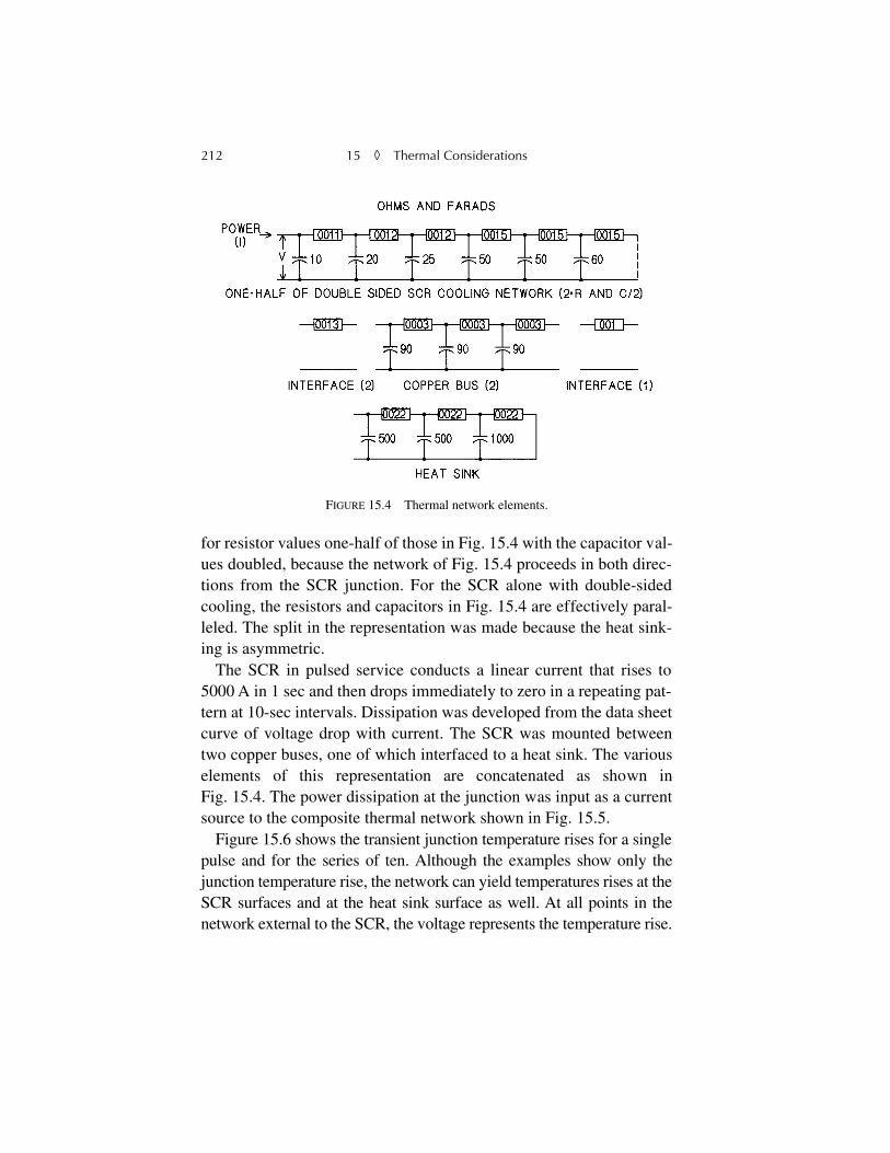
212 15
◊
Thermal Considerations
for resistor values one-half of those in Fig. 15.4 with the capacitor val-ues doubled, because the network of Fig. 15.4 proceeds in both direc-tions from the SCR junction. For the SCR alone with double-sidedcooling, the resistors and capacitors in Fig. 15.4 are effectively paral-leled. The split in the representation was made because the heat sink-ing is asymmetric.
The SCR in pulsed service conducts a linear current that rises to5000 A in 1 sec and then drops immediately to zero in a repeating pat-tern at 10-sec intervals. Dissipation was developed from the data sheetcurve of voltage drop with current. The SCR was mounted betweentwo copper buses, one of which interfaced to a heat sink. The variouselements of this representation are concatenated as shown inFig. 15.4. The power dissipation at the junction was input as a currentsource to the composite thermal network shown in Fig. 15.5.
Figure 15.6 shows the transient junction temperature rises for a singlepulse and for the series of ten. Although the examples show only thejunction temperature rise, the network can yield temperatures rises at theSCR surfaces and at the heat sink surface as well. At all points in thenetwork external to the SCR, the voltage represents the temperature rise.
FIGURE 15.4 Thermal network elements.
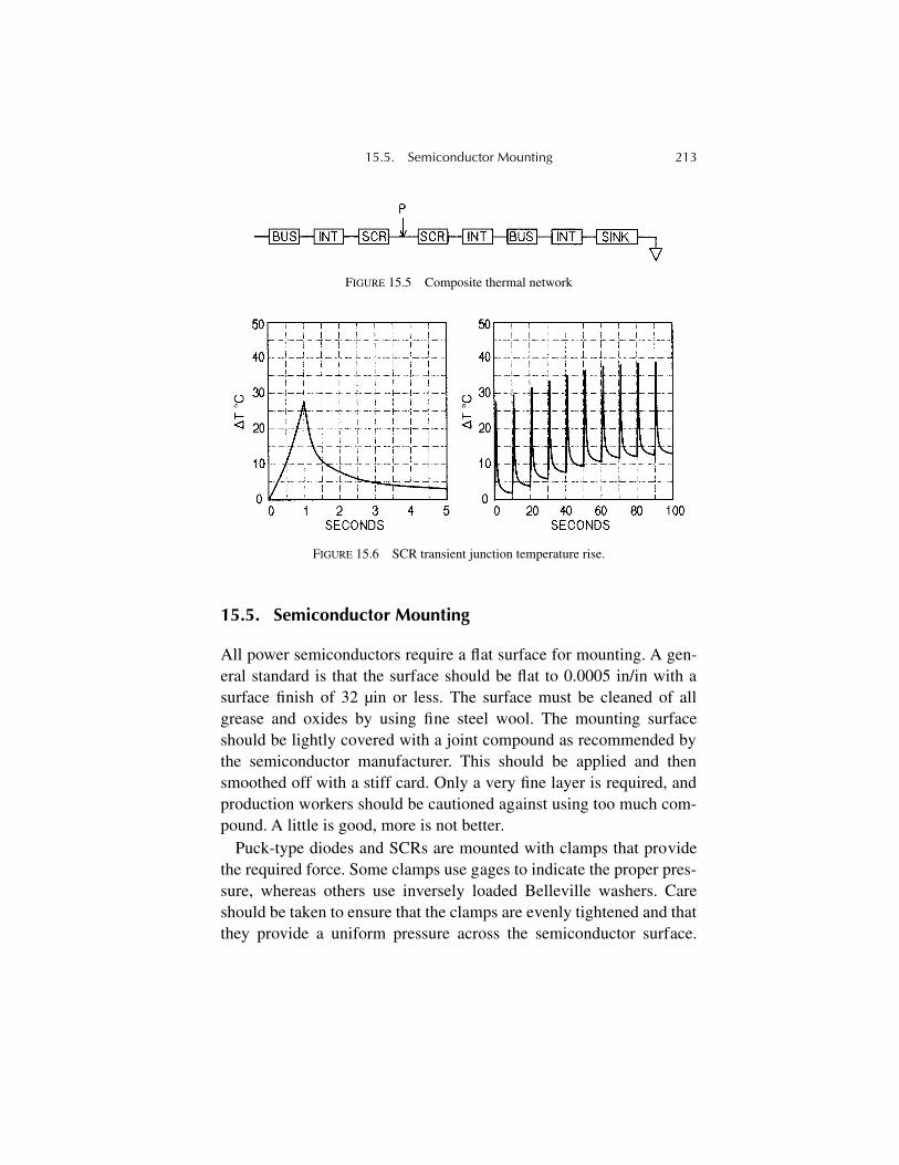
15.5. Semiconductor Mounting 213
15.5. Semiconductor Mounting
All power semiconductors require a flat surface for mounting. A gen-eral standard is that the surface should be flat to 0.0005 in/in with asurface finish of 32 µin or less. The surface must be cleaned of allgrease and oxides by using fine steel wool. The mounting surfaceshould be lightly covered with a joint compound as recommended bythe semiconductor manufacturer. This should be applied and thensmoothed off with a stiff card. Only a very fine layer is required, andproduction workers should be cautioned against using too much com-pound. A little is good, more is not better.
Puck-type diodes and SCRs are mounted with clamps that providethe required force. Some clamps use gages to indicate the proper pres-sure, whereas others use inversely loaded Belleville washers. Careshould be taken to ensure that the clamps are evenly tightened and thatthey provide a uniform pressure across the semiconductor surface.
FIGURE 15.5 Composite thermal network
FIGURE 15.6 SCR transient junction temperature rise.

214 15
◊
Thermal Considerations
One technique is to tighten the nuts on the two sides finger tight,check for even lengths of free bolt threads, and then alternatelytighten the nuts one-half turn at a time until the correct pressure isindicated.
Power IGBTs are housed in epoxy or other molded plastic packageswith an integral mounting plate. Again, joint compound should beused sparingly, but the mounting bolts can be driven tight.
215
Chapter 16
Power Electronics Applications
Power electronics has penetrated nearly every field of humanendeavor. Fuel cells and inverters provide ultra-reliable power for crit-ical industries. Electric utility systems employ HVDC converters andvar compensators to control voltage and power levels. Lamp dimmersallow control of residential lighting levels. Motor drives, the largestuser of power electronics, are at home in pipeline pumping, power sta-tion draft fans, and air conditioning systems. They propel luxurycruise ships and grimy freight locomotives and serve a host of otherapplications. They bring precise speed and torque control with lowerenergy use. IGBT choppers in DC arc furnaces have tamed the powerfactor and flicker problems of AC furnaces and reduced electrode con-sumption. Power electronics is here to stay! Some of the many uses ofpower electronics are described in this chapter.
16.1. Motor Drives and SCR Starters
AC and DC motor drives and SCR starters have been touched on inprevious chapters. Here, some of the applications will be discussed,and variable-speed pumps are a good place to start. Prior to inexpen-sive variable-speed drives, fluid flow in the chemical process indus-tries and municipal water works was controlled by throttling valves on
216 16
◊
Power Electronics Applications
constant-speed pumps. At low flow rates, the pumps were very ineffi-cient, and the lost energy went into heating the fluid. With a variable-speed drive, the pumps can be speed controlled to meet the fluid flowdemand with no loss of efficiency. The same is true for pipeline pump-ing of liquid fuels where the same advantages accrue in drives to10,000 hp.
Centrifuges are used for separating liquefied material mixtures.They must be accelerated as quickly as possible and then deceleratedquickly when the process step is over. Torque controlled, regenerativevariable-speed drives and motors make quick work of the job. Hoistsand elevators can be hoisted smoothly and then regeneratively brakedwith variable-speed drives to save on energy. Dynamometers have thesame requirements. Multiple motors in steel and paper lines can beprecisely controlled with constant, synchronized speeds, and they canmaintain synchronism when accelerating or decelerating.
In the latest diesel electric locomotives, AC inverters power induc-tion motors on the axles. They provide dynamic braking to minimizebrake shoe wear and can immediately reduce torque on a slippingwheel to maintain optimum traction. Induction motors stand up to therigors of railroad service much better than DC motors.
Ventilation systems operating from variable-speed drives do nothave the annoying off-on characteristic of constant-speed fans, sincethey can be continuously speed controlled to maintain the required airflow. Furthermore, they reduce wear and tear on the ventilation sys-tem by eliminating transient starting torques.
Coal-fired electric utility generating stations use variable-speeddrives on forced and induced draft fans for boilers, thereby saving thecost of using throttling methods to control air flow. These units, in the10,000 hp range, offer important economies in power usage. A kilo-watt-hour saved is a kilowatt-hour the utility can sell.
Testing large motor drives is often done with motor generator setsthat allow the drive power to be regenerated back to the power line toreduce costs and eliminate the need for a mechanical brake. Thearrangement is referred to as a
dynamometer
. When the input and out-

16.2. Glass Industry 217
put voltages of a drive are the same, the drive can be tested at full loadand line frequency with a “motorless” dynamometer. A three-phaseinductor is used to couple the drive output back to the power line, andthe drive electronics are phase locked to the line. By displacing therelative phases of the drive and line through the control electronics, afull range of load currents can be obtained. The drive, in effect,becomes a synchronous generator tied to the power line through itsinternal reactance. The cost and losses of a reactor are far less thanthose of a motor generator set, and the only power required is to sup-port the losses of the drive and reactor. An auxiliary transformer canbe used to match voltages when required. This arrangement hasenabled testing of 20,000-hp drives at full load with a 2500-kVA sup-ply rating.
SCR motor starters can often replace variable-speed drives as alower-cost method of controlling starting currents in large AC motors.In fans and pumps, the torque requirements at low speeds are modest,and starting current may be as little as half of the across-the-line start-ing current. Furthermore, the starting current may be ramped up so asto permit coordination with capacitors switched in and out to controlthe voltage.
Another interesting use of AC motor starters is an SCR gating tech-nique that allows the starter to operate induction or synchronousmotors for a short time at very low speeds with high torque. This hasproven useful in rotary kilns and mixers in the cement industry.
16.2. Glass Industry
For over 40 years, the glass industry has used SCR-controlled meltersfor flat glass, container glass, and fiberglass operations. Electric melt-ing reduces dust from gas firing and offers better temperature control.The power controllers must be designed to eliminate any residual DCcomponent in the AC power, because a DC component will cause theelectrodes to plate out into the glass and also produce bubbles, the
218 16
◊
Power Electronics Applications
bane of glass companies. In fact, some companies are using high-fre-quency IGBT supplies for elimination of bubbles in special glasses. Inthe fiberglass industry, SCR controls not only melt and control thetemperature of the glass supply but also control temperatures of thenozzles that spray the fine filaments of glass. These systems utilizepower controllers to 600 V with currents as high as 10 kA.
16.3. Foundry Operations
Furnaces for continuous casting lines, such as those for engineblocks, have a graphite rod above a refractory cupola that is chargedwith molten metal. The electrically heated rod maintains the melt byradiant heat. Power controllers adjust the rod current to maintain anoptimum melt temperature for casting. Since the rod gradually agesto a higher resistance, the supply must operate at constant power overa wide range of load resistances, and the autotapchanger circuit hasbeen popular in these applications. The environment is not friendly toelectrical equipment because of conductive dust that collects oneverything. For this reason, these supplies are totally enclosed,sealed, and water cooled. Figure 16.1 shows a schematic of a typicalinstallation.
Related uses are in annealing wire and strip. Electric heaters annealthe strip by radiant heat, or a current is passed through the material asit travels between roller electrodes and is resistance heated. Both sys-tems have used SCR controllers.
FIGURE 16.1 Rod furnace autotapchanger supply.
16.4. Plasma Arcs and Arc Furnaces 219
16.4. Plasma Arcs and Arc Furnaces
In these special heaters, a feed gas is blown through a high-powerelectric arc to form a superheated plasma. Such systems have beenused to reclaim material from dust formed by blast furnaces and col-lected in precipitators or bag houses. The plasma arc melts the mate-rial before serious oxidation takes place. Power electronics plasma arcsupplies have also been built in power ratings to 25 MW for experi-mental use, one for simulation of reentry heating in space vehicles.
IGBT choppers for DC arc furnaces are being used at 100-MWpower levels. They are able to control the arc current in a millisecondor so and allow the melt to proceed at essentially constant current withimproved throughput. AC arc furnaces must control the arc current byelectrode positioning controls, a slow operation at best. DC furnaceswith chopper control are free from the annoying flicker that AC fur-naces produce, and they also reduce electrode consumption. Thehigher cost of choppers is offset by the fact that DC furnaces do notrequire a var compensator for flicker control, and they operate at abetter power factor. They also can utilize less-expensive power trans-formers, since there is no need for bracing to support short-circuitforces.
16.5. Electrochemical Supplies
The very high-current DC supplies for electrochemical (pot line) usein metals reduction and chlorine production have traditionally usedsilicon rectifiers with saturable reactors and tap-changing transform-ers for continuous current control over a wide range. IGBT choppersare penetrating this field, because they can immediately interruptshort circuits and inherently operate at a good power factor. Further-more, they can be easily modularized for maintenance and reliabil-ity. The chopper supplies are similar to the DC arc furnace choppers.The systems generally use an oil-filled power transformer from theincoming utility supply and a series of phase shifted, water-cooled
220 16
◊
Power Electronics Applications
transformers to power the choppers. Power levels are unlimited. Fig-ure 16.2 shows a typical system with a 24-pulse transformer rectifierand chopper system.
16.6. Cycloconverters
These units are a special case of motor drives, since they can also beused in fixed-frequency applications and can supply high overloadcurrents for protective relay coordination in large installations. Theyare currently used to convert 60 to 25 Hz for the catenary system ofAmtrak in the New York to Boston corridor. Another use is for shippropulsion, where they provide excellent maneuverability. They con-vert a fixed generator frequency to a variable frequency for the pro-peller synchronous motors. As described earlier, they have acted asfrequency changers for 25-Hz plant supplies from the 60-Hz utilities.The only serious barrier to the application of cycloconverters is thatthe output frequency must be less than half of the input frequency toavoid asymmetry of output voltage waveforms. However, they alsooperate at a poor power factor and have an unpleasant series of har-monics and intermodulation products on the incoming power linecurrent. Figure 16.3 shows the basic schematic of a three-phasecycloconverter. Note that the three dual converters are supplied from a
FIGURE 16.2 Typical electrochemical supply.
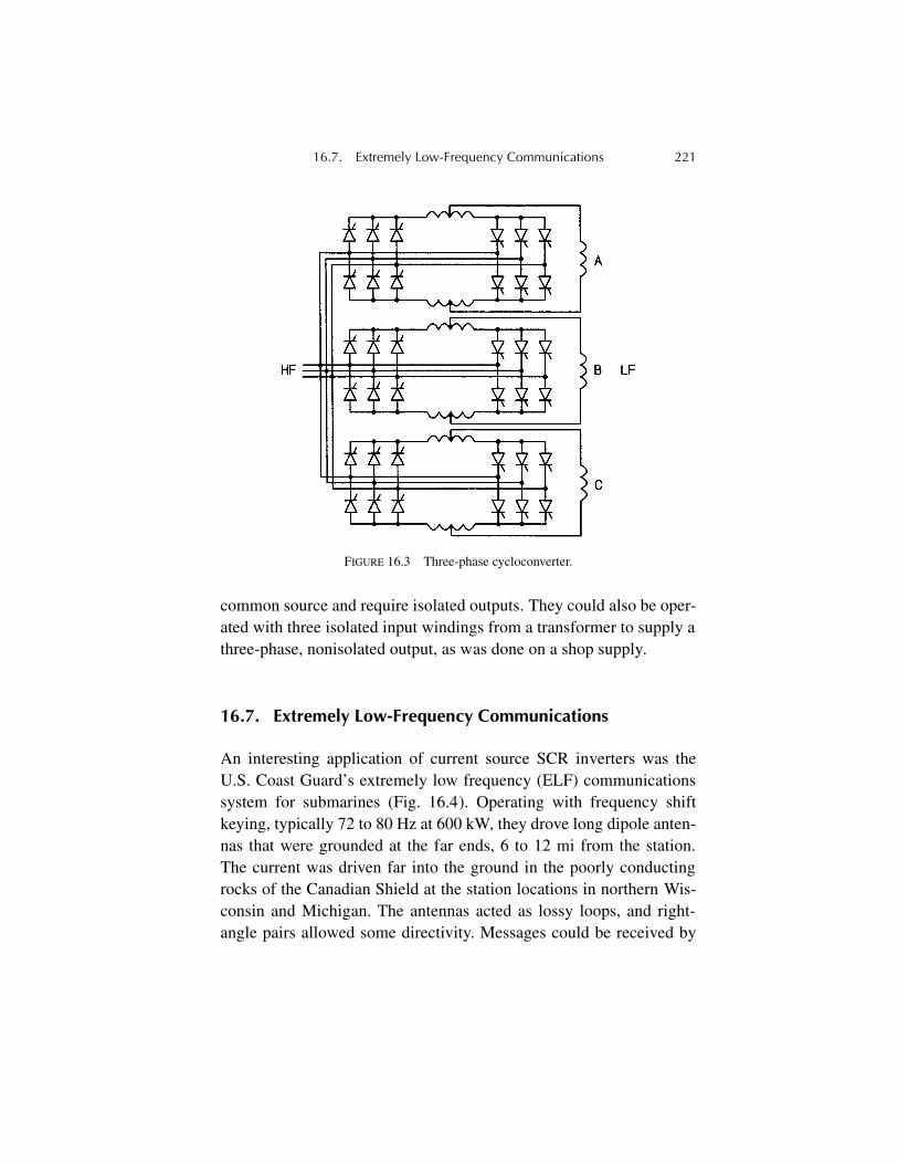
16.7. Extremely Low-Frequency Communications 221
common source and require isolated outputs. They could also be oper-ated with three isolated input windings from a transformer to supply athree-phase, nonisolated output, as was done on a shop supply.
16.7. Extremely Low-Frequency Communications
An interesting application of current source SCR inverters was theU.S. Coast Guard’s extremely low frequency (ELF) communicationssystem for submarines (Fig. 16.4). Operating with frequency shiftkeying, typically 72 to 80 Hz at 600 kW, they drove long dipole anten-nas that were grounded at the far ends, 6 to 12 mi from the station.The current was driven far into the ground in the poorly conductingrocks of the Canadian Shield at the station locations in northern Wis-consin and Michigan. The antennas acted as lossy loops, and right-angle pairs allowed some directivity. Messages could be received by
FIGURE 16.3 Three-phase cycloconverter.
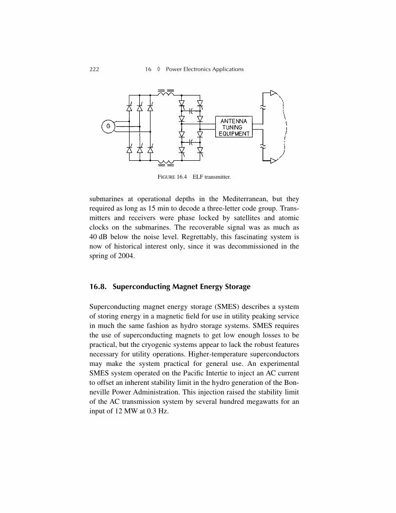
222 16
◊
Power Electronics Applications
submarines at operational depths in the Mediterranean, but theyrequired as long as 15 min to decode a three-letter code group. Trans-mitters and receivers were phase locked by satellites and atomicclocks on the submarines. The recoverable signal was as much as40 dB below the noise level. Regrettably, this fascinating system isnow of historical interest only, since it was decommissioned in thespring of 2004.
16.8. Superconducting Magnet Energy Storage
Superconducting magnet energy storage (SMES) describes a systemof storing energy in a magnetic field for use in utility peaking servicein much the same fashion as hydro storage systems. SMES requiresthe use of superconducting magnets to get low enough losses to bepractical, but the cryogenic systems appear to lack the robust featuresnecessary for utility operations. Higher-temperature superconductorsmay make the system practical for general use. An experimentalSMES system operated on the Pacific Intertie to inject an AC currentto offset an inherent stability limit in the hydro generation of the Bon-neville Power Administration. This injection raised the stability limitof the AC transmission system by several hundred megawatts for aninput of 12 MW at 0.3 Hz.
FIGURE 16.4 ELF transmitter.
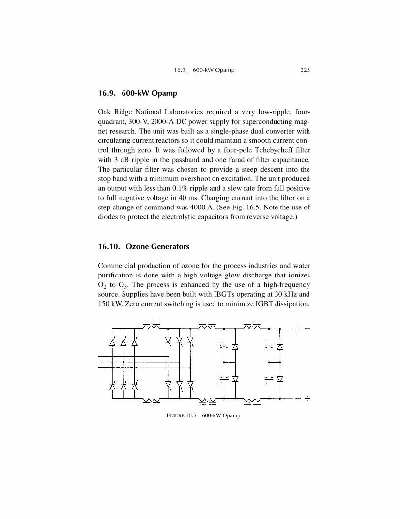
16.9. 600-kW Opamp 223
16.9. 600-kW Opamp
Oak Ridge National Laboratories required a very low-ripple, four-quadrant, 300-V, 2000-A DC power supply for superconducting mag-net research. The unit was built as a single-phase dual converter withcirculating current reactors so it could maintain a smooth current con-trol through zero. It was followed by a four-pole Tchebycheff filterwith 3 dB ripple in the passband and one farad of filter capacitance.The particular filter was chosen to provide a steep descent into thestop band with a minimum overshoot on excitation. The unit producedan output with less than 0.1% ripple and a slew rate from full positiveto full negative voltage in 40 ms. Charging current into the filter on astep change of command was 4000 A. (See Fig. 16.5. Note the use ofdiodes to protect the electrolytic capacitors from reverse voltage.)
16.10. Ozone Generators
Commercial production of ozone for the process industries and waterpurification is done with a high-voltage glow discharge that ionizesO
2
to O
3
. The process is enhanced by the use of a high-frequencysource. Supplies have been built with IBGTs operating at 30 kHz and150 kW. Zero current switching is used to minimize IGBT dissipation.
FIGURE 16.5 600-kW Opamp.
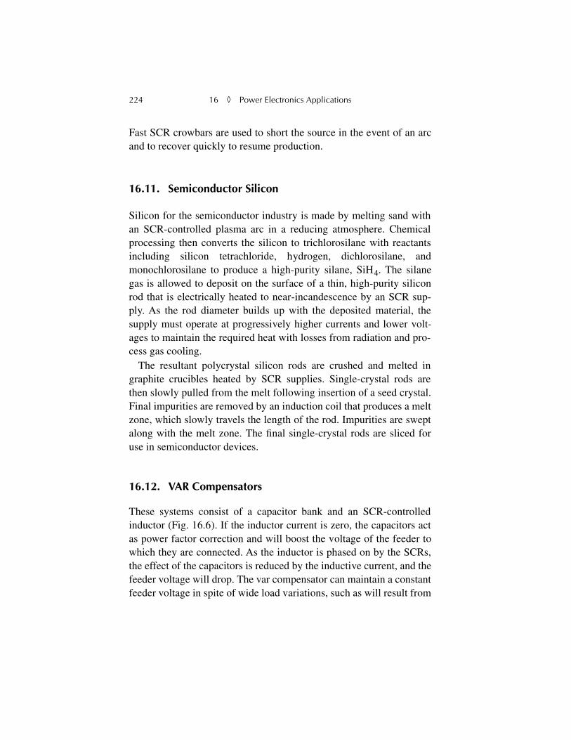
224 16
◊
Power Electronics Applications
Fast SCR crowbars are used to short the source in the event of an arcand to recover quickly to resume production.
16.11. Semiconductor Silicon
Silicon for the semiconductor industry is made by melting sand withan SCR-controlled plasma arc in a reducing atmosphere. Chemicalprocessing then converts the silicon to trichlorosilane with reactantsincluding silicon tetrachloride, hydrogen, dichlorosilane, andmonochlorosilane to produce a high-purity silane, SiH
4
. The silanegas is allowed to deposit on the surface of a thin, high-purity siliconrod that is electrically heated to near-incandescence by an SCR sup-ply. As the rod diameter builds up with the deposited material, thesupply must operate at progressively higher currents and lower volt-ages to maintain the required heat with losses from radiation and pro-cess gas cooling.
The resultant polycrystal silicon rods are crushed and melted ingraphite crucibles heated by SCR supplies. Single-crystal rods arethen slowly pulled from the melt following insertion of a seed crystal.Final impurities are removed by an induction coil that produces a meltzone, which slowly travels the length of the rod. Impurities are sweptalong with the melt zone. The final single-crystal rods are sliced foruse in semiconductor devices.
16.12. VAR Compensators
These systems consist of a capacitor bank and an SCR-controlledinductor (Fig. 16.6). If the inductor current is zero, the capacitors actas power factor correction and will boost the voltage of the feeder towhich they are connected. As the inductor is phased on by the SCRs,the effect of the capacitors is reduced by the inductive current, and thefeeder voltage will drop. The var compensator can maintain a constantfeeder voltage in spite of wide load variations, such as will result from
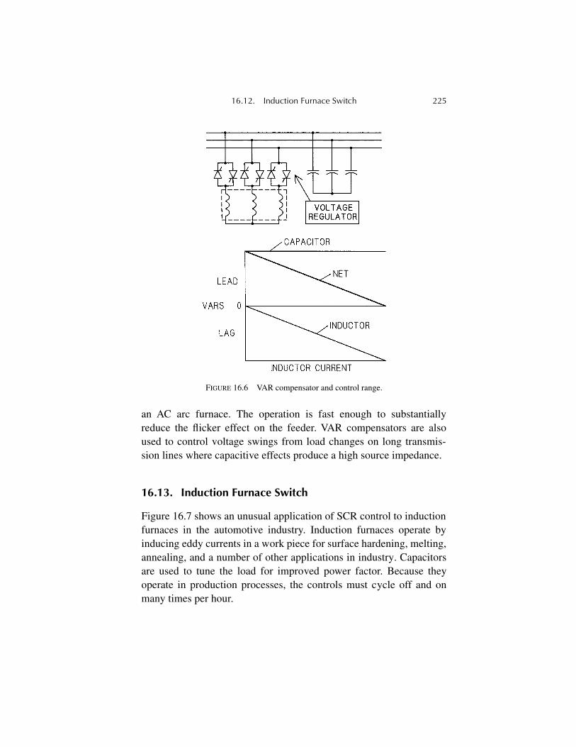
16.12. Induction Furnace Switch 225
an AC arc furnace. The operation is fast enough to substantiallyreduce the flicker effect on the feeder. VAR compensators are alsoused to control voltage swings from load changes on long transmis-sion lines where capacitive effects produce a high source impedance.
16.13. Induction Furnace Switch
Figure 16.7 shows an unusual application of SCR control to inductionfurnaces in the automotive industry. Induction furnaces operate byinducing eddy currents in a work piece for surface hardening, melting,annealing, and a number of other applications in industry. Capacitorsare used to tune the load for improved power factor. Because theyoperate in production processes, the controls must cycle off and onmany times per hour.
FIGURE 16.6 VAR compensator and control range.
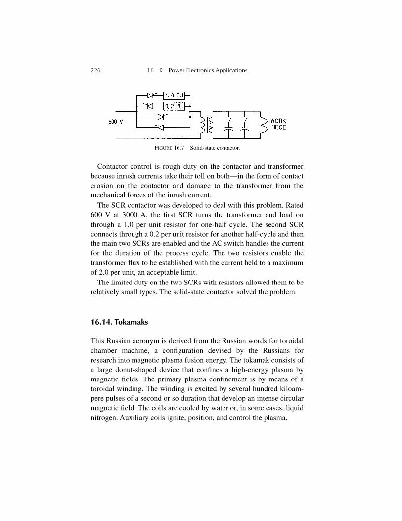
226 16
◊
Power Electronics Applications
Contactor control is rough duty on the contactor and transformerbecause inrush currents take their toll on both—in the form of contacterosion on the contactor and damage to the transformer from themechanical forces of the inrush current.
The SCR contactor was developed to deal with this problem. Rated600 V at 3000 A, the first SCR turns the transformer and load onthrough a 1.0 per unit resistor for one-half cycle. The second SCRconnects through a 0.2 per unit resistor for another half-cycle and thenthe main two SCRs are enabled and the AC switch handles the currentfor the duration of the process cycle. The two resistors enable thetransformer flux to be established with the current held to a maximumof 2.0 per unit, an acceptable limit.
The limited duty on the two SCRs with resistors allowed them to berelatively small types. The solid-state contactor solved the problem.
16.14. Tokamaks
This Russian acronym is derived from the Russian words for toroidalchamber machine, a configuration devised by the Russians forresearch into magnetic plasma fusion energy. The tokamak consists ofa large donut-shaped device that confines a high-energy plasma bymagnetic fields. The primary plasma confinement is by means of atoroidal winding. The winding is excited by several hundred kiloam-pere pulses of a second or so duration that develop an intense circularmagnetic field. The coils are cooled by water or, in some cases, liquidnitrogen. Auxiliary coils ignite, position, and control the plasma.
FIGURE 16.7 Solid-state contactor.
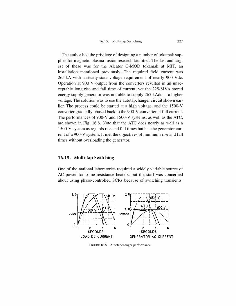
16.15. Multi-tap Switching 227
The author had the privilege of designing a number of tokamak sup-plies for magnetic plasma fusion research facilities. The last and larg-est of these was for the Alcator C-MOD tokamak at MIT, aninstallation mentioned previously. The required field current was265 kA with a steady-state voltage requirement of nearly 900 Vdc.Operation at 900 V output from the converters resulted in an unac-ceptably long rise and fall time of current, yet the 225-MVA storedenergy supply generator was not able to supply 265 kAdc at a highervoltage. The solution was to use the autotapchanger circuit shown ear-lier. The process could be started at a high voltage, and the 1500-Vconverter gradually phased back to the 900-V converter at full current.The performances of 900-V and 1500-V systems, as well as the ATC,are shown in Fig. 16.8. Note that the ATC does nearly as well as a1500-V system as regards rise and fall times but has the generator cur-rent of a 900-V system. It met the objectives of minimum rise and falltimes without overloading the generator.
16.15. Multi-tap Switching
One of the national laboratories required a widely variable source ofAC power for some resistance heaters, but the staff was concernedabout using phase-controlled SCRs because of switching transients.
FIGURE 16.8 Autotapchanger performance.
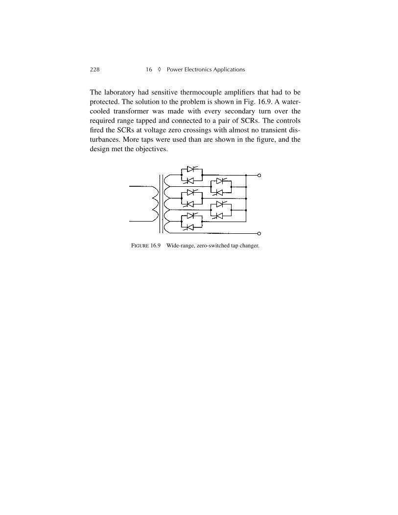
228 16
◊
Power Electronics Applications
The laboratory had sensitive thermocouple amplifiers that had to beprotected. The solution to the problem is shown in Fig. 16.9. A water-cooled transformer was made with every secondary turn over therequired range tapped and connected to a pair of SCRs. The controlsfired the SCRs at voltage zero crossings with almost no transient dis-turbances. More taps were used than are shown in the figure, and thedesign met the objectives.
FIGURE 16.9 Wide-range, zero-switched tap changer.
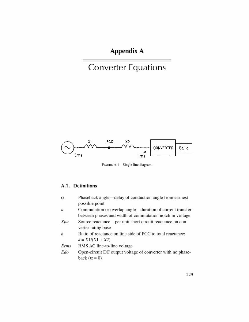
229
Appendix A
Converter Equations
A.1. Definitions
α
Phaseback angle—delay of conduction angle from earliest possible point
u
Commutation or overlap angle—duration of current transfer between phases and width of commutation notch in voltage
Xpu
Source reactance—per unit short circuit reactance on con-verter rating base
k
Ratio of reactance on line side of PCC to total reactance;
k
=
X
1/(
X
1 +
X
2)
Erms
RMS AC line-to-line voltage
Edo
Open-circuit DC output voltage of converter with no phase-back (
α
= 0)
FIGURE A.1 Single line diagram.

230 A
◊
Converter Equations
Ed
DC output voltage under rated loadcos(
ϕ
) Displacement power factor—cosine of angle between funda-mental line-to-neutral voltage and fundamental current
Irms
RMS AC line current
Id
DC load current
Ipu
Per unit AC or DC load current
Ihpu
Per unit harmonic line current at harmonic,
hTHDv
Voltage total harmonic distortion at PCC
Ifpu
Per unit peak asymmetric fault current
PCC
Point of common coupling between utility and customer—usually the metering point
A.2. Equations at Full Load
1
1.
Edo
= 1.35
Erms
2.
Ed
=
Edo
[cos(
α
) –
Xpu
/2)]3.
Ed
=
Edo
(1 –
Xpu
/2) (
α
= 0)4.
Edpu
= cos(
α
) –
Xpu
/25.
Edpu
= 1 –
Xpu
/2 (
α
= 0)6. cos(
α
+
u
) = cos(
α
) –
Xpu
7. cos(
u
) = 1 –
Xpu
(
α
= 0)8. cos(
α
)
≈
cos(
α
+
u
/2) (
α
≠
0)9.
Irms
≈
0.816
Id
10.
Ihpu
= 1/
h
(
h
= 6
n
± 1)11.
TDDv
≈
k
sin(
α
+
u
/2)12.
Ifpu
≈
2/
Xpu
1
Note:
For operation at less than full load, replace
Xpu
in Eqs. 2 through 7 with
Xpu
Ipu
.
u

231
Appendix B
Lifting Forces
Lifting forces on cabinets for handling by a crane can be determinedfrom measurements or calculation of the center of gravity and loca-tion of lifts. The basic consideration is that the moments about thepivot point must always balance. The pivot point is the cabinet endthat remains on the floor with a single lift. One moment is the totalweight, acting at the center of gravity, multiplied by the distance fromthe center of gravity to the pivot point. The other moment is the liftingforce multiplied by the distance from the lift point to the pivot point.These two moments must always be equal. If the total weight and thecenter of gravity are known, the lifting forces can be calculated. If thetwo lifting moments are determined experimentally, the center ofgravity and total weight can be calculated. The following example of adouble lift may help. The lift forces
F
1 and
F
2 and their locations arepresumed known, and the weight,
W
, and center of gravity,
X
, are to befound (Fig. B.1).
B.1. Calculations
M
1 =
W
(
C
–
X
)
M
2 =
F
1
C
at
L
1
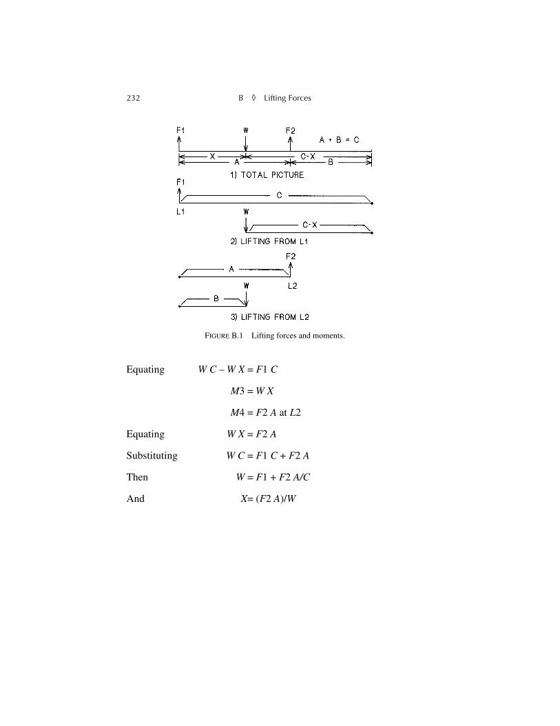
232 B
◊
Lifting Forces
Equating
W
C
–
W
X
=
F
1
C
M
3 =
W
X
M
4 =
F
2
A
at
L
2
Equating
W
X
=
F
2
A
Substituting
W
C
=
F
1
C
+
F
2
A
Then
W
=
F
1 +
F
2
A/C
And
X
= (
F
2
A
)/
W
FIGURE B.1 Lifting forces and moments.
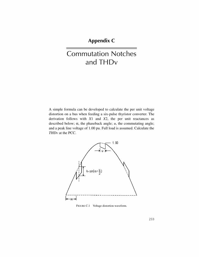
233
Appendix C
Commutation Notches and THDv
A simple formula can be developed to calculate the per unit voltagedistortion on a bus when feeding a six-pulse thyristor converter. Thederivation follows with
X
1 and
X
2, the per unit reactances asdescribed below;
α
, the phaseback angle;
u
, the commutating angle;and a peak line voltage of 1.00 pu. Full load is assumed. Calculate the
THDv
at the PCC.
FIGURE C.1 Voltage distortion waveform.

234 C
◊
Commutation Notches and THDv
1.
k
=
X
1/(
X
1 +
X
2) (
X
1 is the per unit reactance on the line side of the PCC and
X
2 is on the load side).2.
Xc
=
X
1 +
X
2 (commutating reactance)3. cos(
α
+
u
) = cos(
α
) –
Xc.
4. There is one commutation notch determined by
k
and two at half-value as shown in Fig. C.1 in the line-to-line waveform with
k
= 0.33.5. The main notch has an average depth of
k
sin(
α
+
u
/2) and a width of
u
.6. The RMS value of the notches is
k
sin(
α
+
u
/2)
[3
u
/(2
π
)]
1/2
.7. By approximating (3/
π
)
1/2
as 1.0, and dividing by the approxi-mate RMS value of per unit line-to-line voltage as (1/2)
1/2
, the
THDv
becomes
THDv
=
k
sin(
α
+
u
/2)
(
u
)
1/2
with
α
and
u
in radians
235
Appendix D
Capacitor Ratings
ANSI/IEEE Std. 18-1980 specifies that power factor correction capac-itors must be applied within the following guidelines, no one of whichmay be exceeded:
1. RMS voltage not to exceed 110% of rated2. Peak voltage not to exceed 120% of rated3. RMS current not to exceed 180% of rated
1
4. kVA not to exceed 135% of rated
The calculations are to be made as follows:
1. RMS voltage—The RMS applied voltage is the square root sum of squares of all fundamental and harmonic voltages across the capacitor. The fundamental voltage should be taken as the maxi-mum sustained line voltage and must include any voltage rise due to a tuning reactor. Harmonic voltages are calculated from the harmonic currents and the capacitor reactances at harmonic fre-quencies. The RMS voltage limit is associated with dielectric heating effects.
1
Note that some 480-V and 600-V power factor correction capacitors may be limited to135% rated current.
236 D
◊
Capacitor Ratings
2. Peak voltage—The peak voltage is calculated as the peak funda-mental voltage plus the peak effect of all harmonic voltages. In principle, this requires an arithmetic addition of all harmonic voltages since they could, admittedly with a small probability, combine as an additive peak. Common sense, however, would suggest the arithmetic addition of the major harmonic voltages and an RMS combination of the remaining peak harmonic volt-ages. The peak voltage limit is associated primarily with the dielectric and corona stresses.
3. RMS current—The RMS current is the result of fundamental cur-rent and all harmonic currents. The fundamental current must be adjusted for capacitance tolerance and terminal voltage. The cur-rent limit is primarily one associated with foil and terminal heat-ing due to I
2
R losses.4. kVA—The kVA is calculated as the arithmetic sum of RMS volt-
age times RMS current for the fundamental and each harmonic. Capacitive reactances at harmonic frequencies can be used to cal-culate voltages. This limit is sort of a “catch-all” based on experi-ence.
237
Appendix E
Rogowski Coils
Figure E.1 shows the construction of a Rogowski coil, an air-core cur-rent transformer that is especially well suited to measuring ripple cur-rents in the presence of a DC component or measuring pulsedcurrents. The raw output is proportional to the derivative of the cur-rent, and the current can be recovered by an integrator or a low-passfilter. The output voltage is given by
e
= 4
π
×
10
–7
n
×
(
A/s
)
di/dt
(MKS units)
e
= 3.19
×
10
–8
n
(
A/s
)
di/dt
(inches)
FIGURE E.1 Rogowski coil construction.
s = 2π (a + b)/2
A = s w
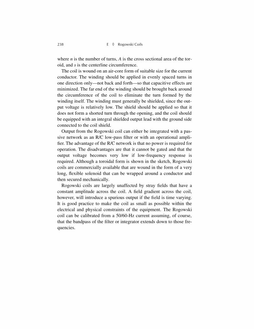
238 E
◊
Rogowski Coils
where
n
is the number of turns,
A
is the cross sectional area of the tor-oid, and
s
is the centerline circumference. The coil is wound on an air-core form of suitable size for the current
conductor. The winding should be applied in evenly spaced turns inone direction only—not back and forth—so that capacitive effects areminimized. The far end of the winding should be brought back aroundthe circumference of the coil to eliminate the turn formed by thewinding itself. The winding must generally be shielded, since the out-put voltage is relatively low. The shield should be applied so that itdoes not form a shorted turn through the opening, and the coil shouldbe equipped with an integral shielded output lead with the ground sideconnected to the coil shield.
Output from the Rogowski coil can either be integrated with a pas-sive network as an R/C low-pass filter or with an operational ampli-fier. The advantage of the R/C network is that no power is required foroperation. The disadvantages are that it cannot be gated and that theoutput voltage becomes very low if low-frequency response isrequired. Although a toroidal form is shown in the sketch, Rogowskicoils are commercially available that are wound in the form of a verylong, flexible solenoid that can be wrapped around a conductor andthen secured mechanically.
Rogowski coils are largely unaffected by stray fields that have aconstant amplitude across the coil. A field gradient across the coil,however, will introduce a spurious output if the field is time varying.It is good practice to make the coil as small as possible within theelectrical and physical constraints of the equipment. The Rogowskicoil can be calibrated from a 50/60-Hz current assuming, of course,that the bandpass of the filter or integrator extends down to those fre-quencies.

239
Appendix F
Foreign Technical Words
T
ABLE
F.1
Foreign Technical Words
English French German Spanish
attention attention Achtung atencióncapacitor condensateur Kondensator capacitorcircuit circuit Strumkreis circuitoconnection connexion Verbindung conexióncurrent courant Strom corrientedanger danger Gefahr peligrofrequency fréquence Frequenz frecuenciagenerator générateur Generator generadorhigh haut hoch alto(a)inductor inducteur Induktor inductorinsulation isolation Isolierung aislamientoinsulator isolateur Isolator aisladormotor moteur Motor motorpower puissance Macht potenciareactor réacteur Reaktor reactorresistor résistance Widerstand resistanciatemperature temperature Temperatur temperaturetorque couple Drehmoment torquetransformer transformateur Transformator transformadortransistor transistor Transistor transistorvoltage tension Spannung voltaje, tensiónwire fil Draht alambre


241
Appendix G
Aqueous Glycol Solutions
Most liquid cooling systems are water based and must be protectedfrom freezing in the northern climates. Ethylene glycol has been thepreferred material in solutions up to about 50% by volume for protec-tion to –40°C. However, more recently, propylene glycol has replacedethylene glycol in many applications, because it is more friendly tothe environment. Slightly more propylene glycol is required for agiven temperature protection. It should be noted that the freezingpoint is the point at which ice crystals first start to form. The solutionwill slush and circulate at somewhat lower temperatures.
Either glycol must be an industrial grade from a chemical supplier.Proprietary mixtures used for automotive and other cooling applica-tions may contain antioxidants or other additives that will increase theconductivity. Glycol mixtures free of additives are generally compati-ble with demineralizer resin beds, although the resin bed vendorshould be consulted.
The two curves below show the freezing points and thermal conduc-tivity of various mixtures of either glycol. These curves have beenderived from published curves based on percent glycol by weight forthe two properties. (See Fig. G.1.)
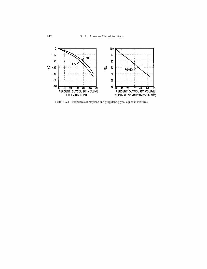
242 G
◊
Aqueous Glycol Solutions
FIGURE G.1 Properties of ethylene and propylene glycol aqueous mixtures.
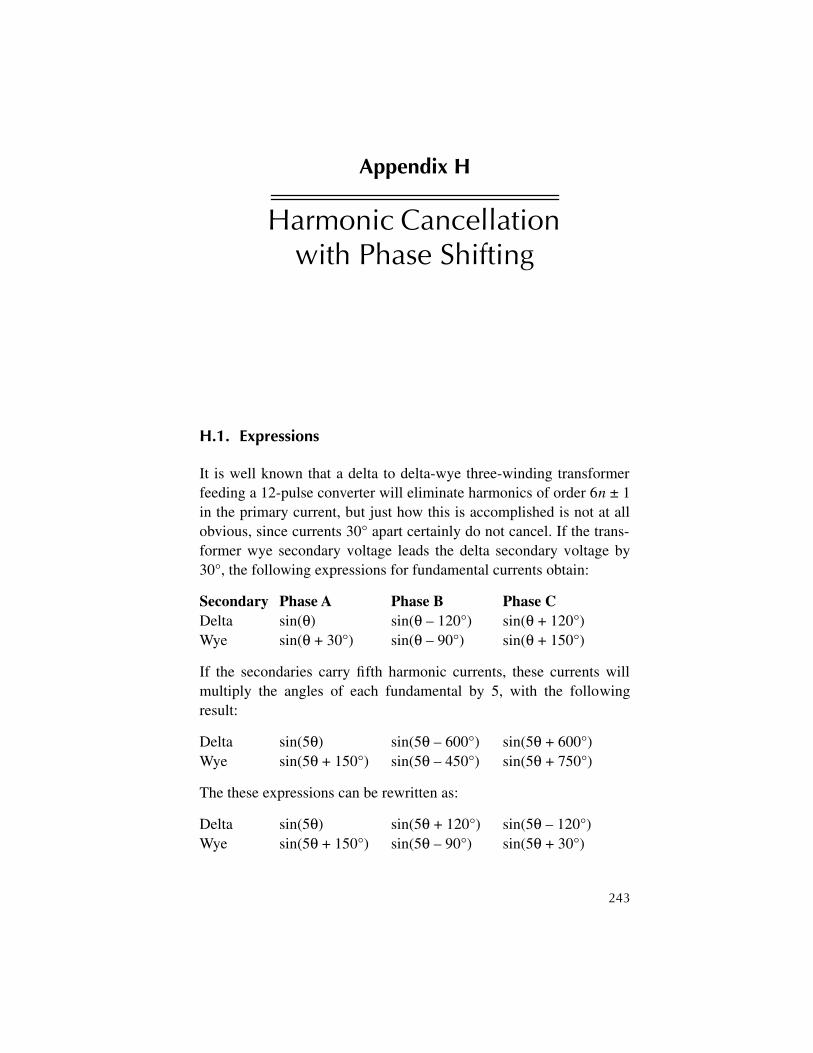
243
Appendix H
Harmonic Cancellation with Phase Shifting
H.1. Expressions
It is well known that a delta to delta-wye three-winding transformerfeeding a 12-pulse converter will eliminate harmonics of order 6
n
± 1in the primary current, but just how this is accomplished is not at allobvious, since currents 30° apart certainly do not cancel. If the trans-former wye secondary voltage leads the delta secondary voltage by30°, the following expressions for fundamental currents obtain:
Secondary Phase A Phase B Phase C
Delta sin(
θ
) sin(
θ
– 120°) sin(
θ
+ 120°)Wye sin(
θ
+ 30°) sin(
θ
– 90°) sin(
θ
+ 150°)
If the secondaries carry fifth harmonic currents, these currents willmultiply the angles of each fundamental by 5, with the followingresult:
Delta sin(5
θ
) sin(5
θ
– 600°) sin(5
θ
+ 600°)Wye sin(5
θ
+ 150°) sin(5
θ
– 450°) sin(5
θ
+ 750°)
The these expressions can be rewritten as:
Delta sin(5
θ
) sin(5
θ
+ 120°) sin(5
θ
– 120°)Wye sin(5
θ
+ 150°) sin(5
θ
– 90°) sin(5
θ
+ 30°)
244 H
◊
Harmonic Cancellation with Phase Shifting
Harmonic currents in the delta secondary lines will become thesame currents in the primary lines. The wye currents, however, willbecome delta currents in the primary, and the primary line current willbe the difference between two wye currents with a ratio of 1/ . Thefollowing equations then apply for primary line currents:
From the delta sin(5
θ
) sin(5
θ
+ 120°) sin(5
θ
– 120°)From the wye (
Ia
–
Ic
)/ (
Ib
–
Ia
)/ (
Ic
–
Ib
)/(Example phase A) [sin(5
θ
+ 150°) – sin(5
θ
+ 30°)]/
Running out the trigonometric relationships shows the fifth harmoniccomponents of line currents from the wye secondary simply wind upas follows:
From the wye –sin(5
θ
) –sin(5
θ
+ 120°) –sin(5
θ
– 120°)
When added to the delta line currents, the fifth harmonic componentsin the line currents vanish identically.
The same kind of analysis will show that the seventh harmonic cur-rents, a positive sequence set, also cancel in the primary, and the sameis true for the 17, 19 pair; the 29, 31 pair; and so on. The remainingharmonics are of order 12
n
± 1. A three-winding transformer is notrequired, nor is the delta-delta-wye configuration. Any windingarrangement that yields a 30° phase shift between load currents willsuffice.
Further work in pushing trigonometric relationships around willshow that a set of 0°, 20°, and 40° phase shifts in three windings willeliminate harmonics except for those of order 18
n
± 1, and that a 0°,15°, 30°, and 45° set will leave only harmonics of order 24
n
± 1. Notethat a set of –22.5°, –7.5°, +7.5°, and + 22.5° will yield identicalresults. The particular set of phase shifts chosen will typically dependon transformer economics. It is the differences that matter.
In the real world, small asymmetries in lines, loads, and transform-ers conspire to prevent a total elimination of these harmonics, but theattenuation is generally enough to bring them into compliance withIEEE 519.
3
3 3 33
245
Appendix I
Neutral Currents with Nonsinusoidal Loads
Single-phase, nonsinusoidal loads in commercial buildings such asdata processing centers cause large neutral currents. These loads havehigh levels of zero sequence triplen harmonics, 3, 9, 15, 21…, andthese harmonics in the line currents are additive in the neutral conduc-tor. The sketch above shows the normal line current waveform and thewaveform as the source inductance approaches zero. In the limit, thecurrent approaches an impulse function with equal current amplitudes
246 I
◊
Neutral Currents with Nonsinusoidal Loads
at all harmonic frequencies. In the worst case, 1 A rms current in eachline becomes 1.732 rms A of current in the neutral. There are one-third as many harmonics in the neutral as in the line current, but eachis three times the amplitude of the line current. Note that the otherodd-order harmonics cancel in the neutral with a balanced load.
Older buildings that were wired with reduced capacity neutral con-ductors in anticipation of reasonably balanced loads with a low har-monic content may face neutral overcurrents when large computerloads are added. The present National Electrical Code recognizes thispossibility and now requires uprated neutrals in new commercial con-struction. These neutral currents will pass through a succession ofwye connected transformers with neutrals, so they may be additive atthe source. Another potential problem is from DC from half-wave rec-tifiers. These currents are also additive in the neutrals, but they willnot pass beyond the first transformer.

247
Index
A
Air cooling 205American Institute of Electrical
Engineers 39ANSI C34.2 92, 122ANSI C57 82ANSI/IEEE Std. 18-1980 235Arc chutes 17Arc heater 43Asynchronous intertie 151Asymptotic response 50Autotapchangers 145Autotransformer 90
B
Basic insulation level, see Insulation, basic insulation level
Bode (bodey) plots 50Bonneville Power Administration 8Boost converter 174Bootstrap circuit 175Bus inductance 158
C
C message weighting 199Canadian General Electric Company
159Canadian Standards Association 22, 34
Capacitorsconstruction 27extended foil 27ratings 235surge 21
Characteristic impedance 66, 67Choppers 173, 215, 219Circular mils 21Coefficient of coupling 74, 75Common-mode voltage 57, 58Commutation 123, 124
failure 141notches 233voltage loss calculation 124
Conductors 12, 21shielded 23
Contactors 18Convection 81, 98, 112, 204Converters 9
boost 174dual arrangement 148equations 229pulsed 163SCR 9
Coolingair 79air-cooled heat sink 205aqueous glycol solutions 241

248 Index
convection 81, 98liquid 25water 206
Corona 8, 33Cosine intercept gate drive 143Crosstalk 86Current source inverter 149Cycloconverters 6, 150, 220
D
Dampers 106Demand charges 9Demineralizer 207di/dt 60Differential-mode voltage 57Direct axis reactance 104Displacement power factor 187Distortion
current and voltage 199limits 201
Distortion factor 192Dog bones 81Dynamometers 216
E
Edison, Thomas 1Electric motors 2, 6Electric utilities 1, 6Electromagnetic interference 61–63,
65, 86, 199–201Electrostatic shield 58, 88ELF communications 221EMALS 112Emissivity 204Energy and demand 182Euler integration 66
F
Faraday screen 58, 88Feedback 103Filter traps 197Flexible AC transmission systems 10,
153
Flux control 110Forward drop 131Fourier transforms 190, 191Fourier, J. B. J. 189Fringing 96Furnaces 219Fuses 24, 31
slo-blo 31
G
Gate drive 127cosine intercept 143
Gate drives 58Gate turnoff thyristor 170Generators 2
turbine 5Glycol 80Grounding 11, 19, 61
straps 33
H
Hall effect 100Harmonic interference 199Harmonic resonance 26Harmonics 26
compensation 196mitigation 193traps 197
Heaviside, Oliver 209Highpass filters 198High-voltage DC 8, 9, 153, 215Hydro-Québec 8
I
IEEE 18-2002 26IEEE 519 119, 186, 200, 244IEEE C57 73Impedance 38Inductance 94
bus 158stray 172
Institute of Electrical and Electronics Engineers 34

Index 249
Insulation 8, 22, 23, 33, 82, 145basic insulation level (BIL) 8, 19,
84, 85classes 82failure 177integrity 88materials 82, 83mineral oil 80temperature considerations 82transformer 84
Integrated gate bipolar transistor 60, 171
Integrated gate controlled thyristor 170
Intermodulation 151Isolation transformers 194
L
Laser 145Lightning arresters 8, 19, 20Load-commutated inverter 149Low-pass filters 198
M
Margin angle 141Metal oxide varistors 17, 35Motor
induction 3synchronous 103, 149
N
National Electric Code 22National Electrical Manufacturers
Association 34, 110Notching 60
O
Oak Ridge National Laboratories 223Overload torque 106Overshoot 69–71Ozone formation 84Ozone generation 223
P
Parasitic heating 25Peak reverse current 128Phase lag 53Phasors 40Power factor 9, 132, 147
correction 19, 25, 183correction capacitors 26definition 181displacement 187true 187
Power resistors, types 30Pulse transformers 154Pulsed converters 163
Q
Quadrature axis reactance 104
R
Rail gun 112, 166Reactance 38, 42, 60, 75, 76, 78, 124,
165, 193, 217direct axis 104quadrature 104subtransient 105synchronous 105
Recovered charge 128Rectifiers
mercury vapor 116multiphase circuits 120single-phase circuits 118vacuum 116
Reflection coefficient 68Regulation 77Relays
designations 38protective 37
Resonanceharmonic 26parallel 26
Responseasymptotic 50frequency 50

250 Index
phase 53time 51
Reverse current 128Ripple 25, 62, 89, 148, 173, 174, 223,
237Rogowski coils 100, 237
S
SCR converters 9, 137, 166SCR starters 133, 135Semiconverter 141Shaft encoder 103Shielded conductors 23Shielding 19, 59, 61, 89Simulation software 47Skirting 98Slip 107Slo-blo fuses 31Snubber 129Spacings, classes 34Specific gravity 204Specific heat 204Stray inductances 172Stress cones 23Subtransient reactance 105Supercaps 171Superconducting magnet energy
storage 222Superconductors 222Switchgear
circuit breakers 11, 17contactors 18electrical clearance 35isolator switches 16load break 17standards 8transfer switches 13
Symbols 15Symmetrical components 39, 41Synchronous motor 103Synchronous reactance 105
T
Tchebycheff filter 223Telephone influence factor 199Tesla, Nikola 3Thermal conductivity 204Tick-tock regulator 169TIF weighting function 199Tokamaks 226Torque 106, 108Total demand distortion 201Total harmonic distortion 192Transformers 3, 164
autotapchanger 147basic arrangements 78connections 90interphase 89isolation 194phase shifting 92pulse 154types and characteristics 81
Transient thermal impedance 208Transients 19Transmission 3, 8Transport lag 43, 54Transposition 86Turbines 5, 7, 101
generator 5wind 110
U
Underwriter’s Laboratories 22, 23, 34, 83
Uninterrupted power 13
V
Vacuum tube rectifiers 116Vector torque control 110Velocity of propagation 67
W
Water cooling 80, 206Westinghouse, George 3