PPG515293 97. - Arko Lucieer - Remote Sensing Scientistlucieer.net/wp-content/uploads/2014/11/2014_Lucieer_PPG_HomeHill.pdf · human casualties and economic losses, largely as damage

http://ppg.sagepub.com/Progress in Physical Geography

http://ppg.sagepub.com/content/38/1/97The online version of this article can be found at:

DOI: 10.1177/0309133313515293

2014 38: 97 originally published online 24 December 2013Progress in Physical GeographyArko Lucieer, Steven M. de Jong and Darren Turner

multi-temporal UAV photographyMapping landslide displacements using Structure from Motion (SfM) and image correlation of

Published by:

http://www.sagepublications.com

can be found at:Progress in Physical GeographyAdditional services and information for

http://ppg.sagepub.com/cgi/alertsEmail Alerts:

http://ppg.sagepub.com/subscriptionsSubscriptions:

http://www.sagepub.com/journalsReprints.navReprints:

http://www.sagepub.com/journalsPermissions.navPermissions:

http://ppg.sagepub.com/content/38/1/97.refs.htmlCitations:

What is This?

- Dec 24, 2013OnlineFirst Version of Record

- Feb 18, 2014Version of Record >>

at Univ. of Tasmania Library on July 13, 2014ppg.sagepub.comDownloaded from at Univ. of Tasmania Library on July 13, 2014ppg.sagepub.comDownloaded from

http://ppg.sagepub.com/

http://ppg.sagepub.com/content/38/1/97

http://www.sagepublications.com

http://ppg.sagepub.com/cgi/alerts

http://ppg.sagepub.com/subscriptions

http://www.sagepub.com/journalsReprints.nav

http://www.sagepub.com/journalsPermissions.nav

http://ppg.sagepub.com/content/38/1/97.refs.html

http://ppg.sagepub.com/content/38/1/97.full.pdf

http://ppg.sagepub.com/content/early/2013/12/20/0309133313515293.full.pdf

http://online.sagepub.com/site/sphelp/vorhelp.xhtml



Article

Mapping landslide displacementsusing Structure from Motion(SfM) and image correlation ofmulti-temporal UAV photography

Arko LucieerUniversity of Tasmania, Australia

Steven M. de JongUtrecht University, The Netherlands

Darren TurnerUniversity of Tasmania, Australia

AbstractIn this study, we present a flexible, cost-effective, and accurate method to monitor landslides using a smallunmanned aerial vehicle (UAV) to collect aerial photography. In the first part, we apply a Structure fromMotion (SfM) workflow to derive a 3D model of a landslide in southeast Tasmania from multi-view UAVphotography. The geometric accuracy of the 3D model and resulting DEMs and orthophoto mosaics wastested with ground control points coordinated with geodetic GPS receivers. A horizontal accuracy of 7 cmand vertical accuracy of 6 cm was achieved. In the second part, two DEMs and orthophoto mosaicsacquired on 16 July 2011 and 10 November 2011 were compared to study landslide dynamics. TheCOSI-Corr image correlation technique was evaluated to quantify and map terrain displacements. Themagnitude and direction of the displacement vectors derived from correlating two hillshaded DEM layerscorresponded to a visual interpretation of landslide change. Results show that the algorithm can accuratelymap displacements of the toes, chunks of soil, and vegetation patches on top of the landslide, but is notcapable of mapping the retreat of the main scarp. The conclusion is that UAV-based imagery in combinationwith 3D scene reconstruction and image correlation algorithms provide flexible and effective tools to mapand monitor landslide dynamics.

KeywordsCOSI-Corr, digital elevation model (DEM), Home Hill landslide, OktoKopter, orthophoto mosaic, Tasmania

I Introduction

Landslides are recognized as an important type

of natural disaster worldwide and are a major

hazard in most mountainous and hilly regions

as well as in steep river banks and coastal slopes

(Dikau et al., 1996; Guzzetti, 2000; Schuster

and Fleming, 1986; Zillman, 1999). Significant

Corresponding author:Arko Lucieer, University of Tasmania, School ofGeography and Environmental Studies, Private Bag 76,Hobart, Tasmania 7001, Australia.Email: [email protected]

Progress in Physical Geography2014, Vol. 38(1) 97–116ª The Author(s) 2013

Reprints and permission:sagepub.co.uk/journalsPermissions.nav

DOI: 10.1177/0309133313515293ppg.sagepub.com

at Univ. of Tasmania Library on July 13, 2014ppg.sagepub.comDownloaded from

http://www.sagepub.co.uk/journalsPermissions.nav

http://ppg.sagepub.com


human casualties and economic losses, largely

as damage to infrastructure (roads, railways,

pipelines, artificial reservoirs) and property

(buildings, agricultural land), have been the

result of mass wasting processes. Landslides are

generally induced when the shear stress on the

slope material exceeds the material’s shear

strength and can be triggered by intense short-

period or prolonged rainfall, earthquakes, or

human activities (Nadim et al., 2006; Swiss

Re, 2011a, 2011b; Varnes and IAEG, 1984).

A significant degree of the damage and a con-

siderable proportion of the human loss associ-

ated with earthquakes and storm events are

caused by landslides as tragically demonstrated

during major events in China in 2008 (Dai et al.,

2011; Gorum et al., 2011) and Brazil in 2011

(Avelar et al., 2013). There is a need to improve

our understanding of landslide processes, iden-

tify the mechanisms that trigger landslides,

develop methods for landslide susceptibility

mapping, keep historic records of landslides,

and develop flexible and reliable monitoring

methods. During the last decade there has been

an increase in the use of remote sensing technol-

ogy for mapping and monitoring of landslides.

There has been a significant improvement in the

spatial resolution of remote sensing technology

in particular with the introduction of laser scan-

ning (both airborne and terrestrial) (Razak et al.,

2011) and unmanned aerial vehicles (UAVs)

(Niethammer et al., 2012). This paper describes

an image-processing workflow based on the

combined use of UAVs, computer vision, and

image correlation techniques for detailed moni-

toring of landslides, however, we first review

the key remote sensing techniques used for

landslide mapping moving from coarse to fine

resolutions.

A wide range of spatial and temporal scales

and a variety of spaceborne, airborne, or

ground-based remote sensing techniques like

optical sensors, thermal, LiDAR, and micro-

wave sensors have been applied for studying

landslides (Delacourt et al., 2007; van Westen

et al., 2008). Earth observation methods are use-

ful to produce detailed multi-temporal sets of

images, orthophotos, and digital elevation mod-

els (DEMs). These products may provide us

with insight into the flow kinematics such as flow

rate, landslide expansion, and accumulation at

the toe zone or retreating scarps. In addition,

these new techniques allow volume calculations

of the accumulated and removed material by

the landslide and mapping of the topographic

changes (McKean and Roering, 2004; Ventura

et al., 2011). Key examples of spaceborne remote

sensing techniques based on optical and RADAR

sensors for landslide studies are reviewed in Guz-

zetti et al. (2012), Joyce et al. (2009), and Metter-

nicht et al. (2005).

Detailed three-dimensional (3D) information

on the land surface can be obtained with laser

scanning techniques, such as airborne LiDAR

and terrestrial laser scanning (TLS) (Glenn

et al., 2006; McKean and Roering, 2004; Razak

et al., 2011; Ventura et al., 2011). Razak et al.

(2011) succeeded in mapping scars and escarp-

ments of a landslide and its dynamics under for-

ests from a time series of very high resolution

airborne LiDAR (140 points per m2). TLS is a

ground-based laser scanning technique to mea-

sure the position and dimension of objects in

3D space. Landslide movements can be detected

by comparing sequential scans; for example,

Abellan et al. (2009, 2010) successfully used

TLS to quantify volumes and frequencies of

rockfall from landslides and steep cliffs.

Dewitte et al. (2008) used stereo photogram-

metry applied to historical aerial photographs to

produce DEMs and in combination with a

LiDAR DEM they tracked small landslide dis-

placements. Fiorucci et al. (2011) analysed

time series of airborne and spaceborne optical

images and used this data set to prove the sea-

sonal behaviour of landslide activity and the

relation with rainfall events in central Italy.

Recently, Travelletti et al. (2012) successfully

applied image correlation techniques on

ground-based images to calculate the

98 Progress in Physical Geography 38(1)



displacements of the Super-Sauze landslide in

the French Alps.

Although spaceborne and airborne remote

sensing techniques are widely used for studying

landslides, these Earth observation methods are

not as flexible as the novel remote sensing plat-

form of unmanned aerial vehicles (UAVs).

Spaceborne and airborne image acquisitions

require thorough planning and might be ham-

pered by unfavourable weather conditions or

other campaigns with higher priorities. Recent

developments in UAV technology provide

exciting new opportunities for ultra-high resolu-

tion (1–20 cm resolution) mapping and monitor-

ing of the environment. The key advantages

of UAVs for environmental remote sensing

include their superior spatial resolution, the

capacity to fly on-demand at critical times, and

their capability of carrying multiple sensors.

UAV-mounted sensors are ideal tools to map

and monitor dynamic features at the Earth sur-

face, such as river channel vegetation (Dunford

et al., 2009), rangeland vegetation (Laliberte

and Rango, 2009; Laliberte et al., 2010, 2011),

Antarctic moss beds (Lucieer et al., 2014;

Turner et al., 2012), crop health status (Zarco-

Tejada et al., 2011), and saltmarsh vegetation

(Kelcey and Lucieer, 2012). UAVs provide a

convenient remote sensing platform for land-

slide studies given their ability to collect ultra-

high resolution imagery over terrain that is often

difficult to access. Furthermore, UAV observa-

tions may bridge the gap between terrestrial

observations and satellite or full-scale airborne

observations. UAV-mounted sensors are not

new, but advances in technology like small,

lightweight UAVs capable of carrying a consid-

erable payload, lightweight cameras, GPS, and

autopilots combined with advanced software

allowing accurate geocoding of imagery have

given a boost to these developments (Dunford

et al., 2009; Neitzel and Klonowski, 2011).

In addition to UAV technology, recent

advances in photogrammetric image processing

and computer vision have resulted in a

technique known as Structure from Motion

(SfM) (Snavely et al., 2008). Highly detailed

3D models can be obtained from overlapping

multi-view photography with SfM algorithms.

Even though the technique was originally

designed for 3D reconstructions of building

facades (e.g. Furukawa and Ponce, 2010; Sna-

vely et al., 2008) and archaeological sites (e.g.

Verhoeven, 2011), more recently the technique

has been successfully applied in Earth sciences

for flexible and cost-effective mapping of a

range of object scales ranging from individual

rock samples to entire landscapes. James and

Robson (2012) demonstrated the application

of SfM in three case studies: a geological rock

sample (0.1 m sample size), a coastal cliff (50

m size), and a crater landscape (1600 m size).

Westoby et al. (2012) used SfM techniques to

map the 3D structure of a steep alpine hill slope

and demonstrated that the SfM-derived eleva-

tion measurements were within 0.1 m of a TLS

scan. Fonstad et al. (2013) also showed accurate

SfM results for geomorphological mapping in

comparison with on-ground GPS (<0.1 m error

in X, Y, and Z) and airborne LiDAR surveys.

In combination with UAV technology, SfM

can provide a cost-effective and efficient means

to acquire dense and accurate 3D data of the

Earth surface. d’Oleire-Oltmanns et al. (2012)

demonstrated the use of a small fixed-wing

UAV for mapping and monitoring soil erosion

in Morocco. Flying at 70 m above ground level

(AGL) they achieved accuracies better than 3

cm using SfM techniques. Harwin and Lucieer

(2012) achieved accuracies between 2.5 and 4

cm when mapping a coastal cliff with a multi-

rotor UAV and an SfM workflow. Turner

et al. (2012) and Lucieer et al. (2014) used a

multi-rotor UAV and SfM workflow to derive

DEMs and orthomosaics of Antarctic moss beds

achieving absolute geometric accuracies of

4 cm compared with DGPS ground control.

Carvajal et al. (2011) demonstrated the use of

a small quadcopter UAV for surveying land-

slides in a road embankment. They achieved

Lucieer et al. 99



planimetric accuracies of *0.5 m and a height

accuracy of 0.11 m. The application of UAVs

and SfM for landslide mapping was elegantly

demonstrated by Niethammer et al. (2010,

2012) who employed a quadcopter UAV to

acquire aerial photography and generated DSMs

and orthomosaics of the Super-Sauze landslide in

southern France based on photogrammetric tech-

niques achieving geometric accuracies of around

0.5 m. Niethammer et al. (2012) also used multi-

temporal UAV orthomosaics to visually identify

and quantify changes in the landslide. Our study

aims to build on this work by automating the

change detection process with image correlation

techniques.

The work by Niethammer et al. (2012) and

Travelletti et al. (2012) inspired us to combine

UAV SfM mapping of landslides with semi-

automated image correlation analysis to quantify

landslide dynamics. In this paper, we illustrate a

workflow showing how UAV-acquired images

can be processed into high resolution DEMs

and orthomosaics used for quantifying landslide

dynamics based on multi-temporal image corre-

lation. The objectives of this paper are:

� to illustrate how time series of digital

photographs acquired over an active land-

slide by a flexible and cost-effective UAV

can be converted into very detailed 3D

point clouds, DEMs, and orthomosaics

using on-board GPS and field DGPS

observations;

� to show how these orthomosaics and

DEM-derived products can be used to

quantify and map the dynamics of a

landslide.

II Research design and methods

1 Study area

To demonstrate the SfM and image correlation

techniques described in this study we selected

an active rotational slump as the main trial site.

The Home Hill landslide is located on the north-

ern flanks of the Huon valley in southern

Tasmania approximately 35 km southwest of

Hobart at an elevation of approximately 80 m

above sea level (Figures 1 and 2). At the top

of the slope the landslide is a rotational earth

slide and downhill it develops into an earth

flow. The dimensions of the landslide are

approximately 125 m by 60 m and it has

developed in strongly weathered, layered fine

colluviums which are remains of underlying

Permian mudstone and siltstone estimated to

be 4–5 m deep (McIntosh et al., 2009). Land use

is pasturage and no trees are present on the

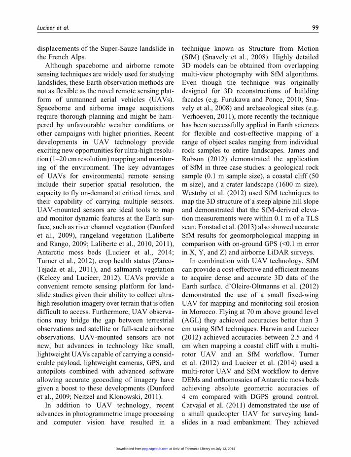
Figure 1. Overview of the Home Hill landslide located in southern Tasmania. The height of the scarp(head wall) is 4–5 m.




slope. The landslide developed in 1996 and is

still active. Field and aerial surveys revealed

that the main scarp developed 5 m backwards

and the northern toe extended approximately

4–5 m between 19 July 2011 and 10 November

2011. The surface of the slide also showed sig-

nificant dynamics including downward shifting

movements and tumbling and overturning of

blocks. Figure 2 shows an aerial photograph

(orthomosaic) of the landslide acquired by our

UAV. The main scarp is clearly visible with a

vertical wall of approximately 4–5 m. Two

landslide toes are visible from which the small

northern toe is most active.

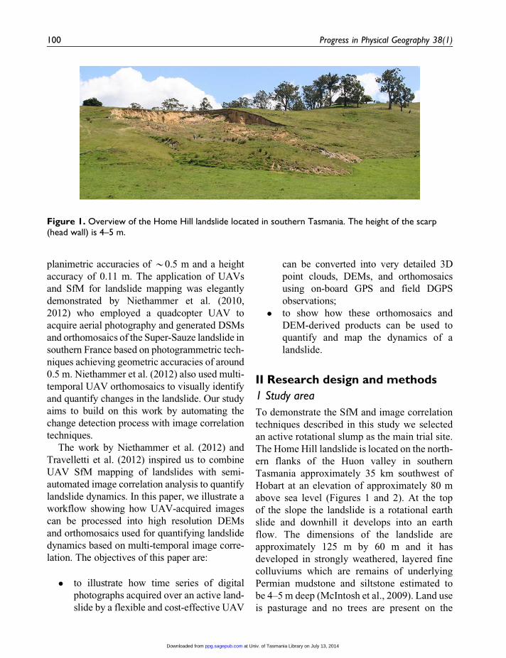
Figure 2. Location map and orthophoto mosaic acquired by UAV of the Home Hill landslide in Tasmania on19 July 2011. The locations of the 24 GCPs used for the SfM bundle adjustment are shown as white disks. The39 GPS samples used for independent accuracy assessment are shown as smaller coloured circles depictingtheir horizontal errors.

Lucieer et al. 101



2 UAV aerial survey

Airborne digital photographs over the landslide

were acquired on two dates, 19 July 2011 and 10

November 2011, using a small multi-rotor

UAV. An OktoKopter is a multi-rotor helicopter

with eight rotors, also classified as a micro-

UAV. Our OktoKopter (Figure 3) is approxi-

mately 80 cm in diameter and has a total

take-off weight of 3 kg. It is equipped with an

autopilot and navigation-grade GPS receiver.

It carries a standard Canon 550D DSLR camera

on a motion-compensated gimbal mount.

A Canon 18–55 mm f3.5–5.6 IS lens was used

given its low weight. The lens was fixed to a

focal length of 18 mm during flight and oper-

ated in autofocus mode. The camera was set to

shutter priority with a fast shutter speed of

1/1200 to reduce motion blur. The ISO was set

to 200 to limit noise in the photographs and the

aperture was automatically adjusted by the cam-

era to achieve the desired shutter speed, but

generally large apertures were selected with

f-values around 3.5. The camera was triggered

by the flight controller every *1.5 seconds by

a custom-made trigger cable. The UAV flight

path was recorded by the on-board GPS logging

at 1 Hz. The average flying height was 40 m

above ground level (AGL) guided by the autop-

ilot. Each 18 megapixel photograph covered

approximately 50�34 m on the ground resulting

in 1 cm resolution imagery. On 19 July 2011

238 UAV photographs were collected, and on

10 November 2011 224 photographs were col-

lected for processing. Despite the impact of rel-

atively strong wind gusts (*25 knots on 10

November 2011) on the UAV platform, we show

here that it is possible to produce accurate image

products. We had overcast and diffuse sunlight

on 19 July 2011 and scattered clouds with vary-

ing light conditions on 10 November 2011.

A visual selection of the photographs was made

on the basis of quality, viewing angle, and over-

lap for further processing, i.e. blurred images and

under- or overexposed images were removed

from further analyses, resulting in 98 photo-

graphs for the July flight and 118 photographs for

the November flight. During UAV data acquisi-

tion 24 circular, aluminium reference disks with

a 22 cm diameter, bright orange rim, and a

clearly defined centroid (visible as a single black

pixel in the images) were laid out around the

landslide for georeferencing purposes (GCPs) for

both UAV survey dates. Another 39 aluminium

orange disks with a 10 cm diameter were spread

out across the landslide for accuracy assessment

purposes on the 19 July 2011 survey. The disks

were manually identified in the UAV imagery for

georeferencing and validation. The disk loca-

tions were measured in the field directly after

UAV image acquisition using a Leica Viva

GNSS system in dual-frequency real-time kine-

matic mode, providing centimetre positional and

height accuracies (2–4 cm).

3 Structure from Motion (SfM) for3D model generation

The SfM process starts by acquiring photo-

graphs of the object of interest with sufficient

overlap (e.g. 80–90%) from multiple positions

and/or angles. Based on advances in image

feature recognition, such as the scale invariant

feature transform (SIFT) (Lowe, 2004), charac-

teristic image objects can be automatically

Figure 3. The remote controlled UAV OktoKopterequipped with digital camera and GPS.




detected, described, and matched between

photographs. A bundle block adjustment is then

performed on the matched features to identify

the 3D position and orientation of the cameras,

and the XYZ location of each feature in the

photographs resulting in a sparse 3D point cloud

(Snavely et al., 2008; Triggs et al., 2000). A sub-

sequent densification technique can then be

applied to derive very dense 3D models using

multi-view stereopsis (MVS) or depth mapping

techniques (Campbell et al., 2008; Furukawa

and Ponce, 2009, 2010). The use of ground con-

trol points (GCPs) and/or incorporation of cam-

era GPS locations allows georeferencing of the

3D model in a real-world coordinate system.

Finally, the model can be exported to a grid-

based DEM and orthophoto mosaics (orthomo-

saics) can be derived based on the projected and

blended photographs.

In this study, we adopted the SfM workflow

as implemented in the commercial software

package Agisoft PhotoScan Professional ver-

sion 0.85.2 The specific algorithms implemen-

ted in Photoscan are not detailed in the

manual, however, a description of the SfM pro-

cedure in Photoscan and commonly used para-

meters are described in Verhoeven (2011) and

Doneus et al. (2011). The algorithms in Photo-

scan are highly optimized for the graphics pro-

cessing unit (GPU). We followed the SfM

workflow described below.

Image preparation. After visual pre-selection,

coordinates were assigned to the UAV-acquired

images. GPS points registered on-board the UAV

were linked to the photographs using the time

settings of the digital camera, which was syn-

chronized with GPS time immediately before the

UAV flight. The technique takes the 1 Hz

sampled GPS points and interpolates the photo-

graph location (coordinates) from the UAV flight

path. For this process we used the GeoSetter

freeware (www.GeoSetter.de) to write the UAV

GPS coordinates to the corresponding JPEG

EXIF headers, i.e. geotagging. Lens distortion

parameters were calculated using an on-screen

lens calibration procedure implemented in the

AgiSoft lens calibration software, which models

the focal length, principal point coordinates, and

radial and tangential distortion coefficients using

Brown’s distortion model. We acknowledge that

these lens distortion coefficients vary for differ-

ent focus distances. We therefore used the coef-

ficients as an initial estimate, but we did not fix

the coefficients in the bundle adjustment.

Image matching and bundle block adjustment. We

imported the pre-selected geotagged photo-

graphs into Photoscan. The photographs were

aligned with the accuracy setting set to high

with the pair pre-selection based on image GPS

coordinates as stored in the JPEG EXIF head-

ers. Attaching GPS coordinates to the photo-

graphs speeds up the feature-matching

process as Photoscan can pre-position the

images and only match features in photographs

that overlap. Feature matching is followed by a

bundle block adjustment. Obvious outliers

were deleted from the sparse point cloud to

reduce reconstruction errors.

Dense geometry reconstruction and inclusion ofGCPs. A dense 3D model was built using

‘height field’ as the object type, the geometry

type was set to smooth, and the target quality

was set to medium with a face count limited

to 10 million faces (i.e. number of triangles).

This resulted in a 3D model that could be

used to manually identify the 24 GCP disks

in the model and the corresponding photo-

graphs. The 3D model can be used to ‘roughly’

position GCP markers in the centroid of the

disks after which the exact position of the mar-

kers can be fine-tuned in the individual photo-

graphs. Based on the field-measured GPS

coordinates of the GCPs, the bundle adjustment

was recalculated with estimated accuracy set-

tings of the camera GPS coordinates set to

10 m and the ground GCPs set to 2 cm. Photo-

scan uses both sets of GPS coordinates with

Lucieer et al. 103



their estimated accuracy to fine-tune the bundle

adjustment. Residuals for the GCPs were calcu-

lated as an initial indication of the geometric

accuracy of the model. Based on the updated

bundle adjustment, the dense 3D geometry was

recomputed with the target quality set to high,

again with a target face count for the model of

10 million.

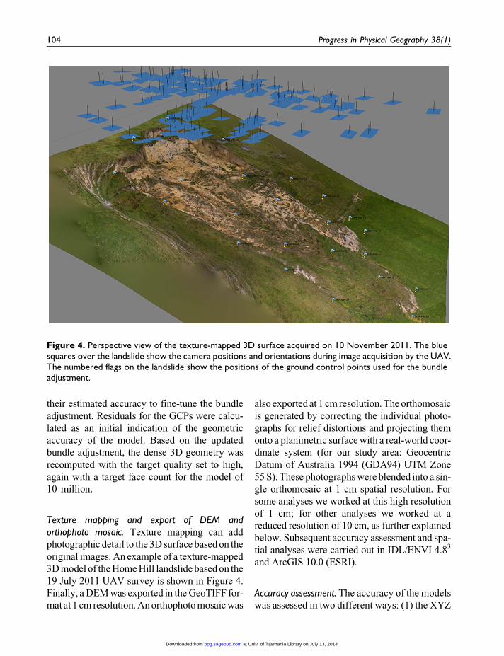
Texture mapping and export of DEM andorthophoto mosaic. Texture mapping can add

photographic detail to the 3D surface based on the

original images. An example of a texture-mapped

3D model of the Home Hill landslide based on the

19 July 2011 UAV survey is shown in Figure 4.

Finally, a DEM was exported in the GeoTIFF for-

mat at 1 cm resolution. An orthophoto mosaic was

also exported at 1 cm resolution. The orthomosaic

is generated by correcting the individual photo-

graphs for relief distortions and projecting them

onto a planimetric surface with a real-world coor-

dinate system (for our study area: Geocentric

Datum of Australia 1994 (GDA94) UTM Zone

55 S). These photographs were blended into a sin-

gle orthomosaic at 1 cm spatial resolution. For

some analyses we worked at this high resolution

of 1 cm; for other analyses we worked at a

reduced resolution of 10 cm, as further explained

below. Subsequent accuracy assessment and spa-

tial analyses were carried out in IDL/ENVI 4.83

and ArcGIS 10.0 (ESRI).

Accuracy assessment. The accuracy of the models

was assessed in two different ways: (1) the XYZ

Figure 4. Perspective view of the texture-mapped 3D surface acquired on 10 November 2011. The bluesquares over the landslide show the camera positions and orientations during image acquisition by the UAV.The numbered flags on the landslide show the positions of the ground control points used for the bundleadjustment.




residuals for the 24 GCP disks were calculated

in Photoscan as part of the bundle adjustment

and model generation process; (2) an indepen-

dent validation was carried out with the 39

smaller disks for the 19 July 2011 UAV survey.

These disks were identified in the orthomosaic

and the error in X and Y measured. The differ-

ence in height was measured on the DEM. Sum-

mary statistics, such as minimum, maximum,

mean error, standard deviation, and root mean

squared error (RMSE), were calculated to quan-

tify geometric accuracies.

3 Visual interpretation of surface dynamics

The dynamics of the landslide between two

acquisition dates were visually investigated by

overlaying two orthomosaics in RGB combina-

tions in an image-processing system (ENVI). One

band of the first image, for example green for 19

July 2011, was assigned to the red channel, and

the green band of the second image (10 November

2011) was assigned to the green and blue chan-

nels. Such colour combinations allow easy recog-

nition of the displacements on screen. Next, using

a measuring tool, the displacement magnitudes

(in metres) and the displacement directions were

mapped for clearly identifiable features on the

landslide. The measurements include the retreat

of the main scarp, the extension of the two toes

of the landslide, and the displacements of identi-

fiable features on the surface of the slide such as

circular patches of grass and ground lobes.

4 Image correlation and displacementsmeasurements

After precise co-registration of the UAV ortho-

mosaics, the horizontal dynamics of the landslide

were determined using an advanced image corre-

lation method developed by LePrince et al.

(2007, 2008). The method is referred to as

COSI-Corr: Co-registration of Optically Sensed

Images and Correlation (Ayoub et al., 2009).4

It considers two single-band images of any

source, such as optical satellite images acquired

by ASTER (Herman et al., 2011) and by SPOT

(Leprince et al., 2007) or DEMs derived from

SRTM or ASTER (Scherler et al., 2008). COSI-

Corr can also work with orthorectified aerial

photography, such as our UAV orthomosaics.

Since the algorithm works on single-band images,

the multi-band RGB image must be converted to a

single-band image. In this study, we evaluated the

following single-band images for displacement

mapping: the individual colour bands (red, green

and blue); the first and second principal compo-

nent images (the third PC image was too noisy for

analysis); colour transformed images – hue,

saturation and value (i.e. luminosity grey-scaling)

images; the average DN-value in the three RGB

bands; and a DEM-derived product – the shaded

relief map. The hillshade operator was applied

with a sun elevation of 45� and an azimuth of

315�. These illumination conditions are represen-

tative of the solar position during a typical sum-

mer afternoon. The azimuth of the light source

corresponds to the general northwest to southeast

direction of the landslide. The artificial lighting in

the hillshade operator should therefore highlight

the main terrain features, such as lobes and fis-

sures in the main flow direction of the landslide.

COSI-Corr uses an image kernel to compute

the correlation between the two images. Two

correlation algorithms are proposed by

LePrince et al. (2007). The first is a frequency

correlation method computing the relative dis-

placement between the pair of images retrieved

from a Fourier transform. The second is a statis-

tical correlation method defined as the absolute

value of the correlation coefficient of a patch in

one image and the corresponding patch in the

other image. The estimated misregistration or

displacement, expressed in pixels, is found from

quadratic approximation, separately in each x

and y dimension, of the maximum of the corre-

lation matrix. A typical correlation analysis is

performed using window sizes of 128 down to

32 pixels, steps of 4 pixels between adjacent

correlations, and a search radius of a few metres,

Lucieer et al. 105



but this requires heuristic fine tuning. The input

images should be co-registered as accurately as

possible as the correlation algorithm is sensitive

to image misregistration errors. In addition,

image noise due to striping and sensor noise, but

also illumination differences (e.g. caused by

clouds and shade), will have a deteriorating

effect on the displacement analysis.

The displacement algorithm in COSI-Corr

requires a number of initial settings (Ayoub

et al., 2009): (1) window size – the size in pixels

of the patches that will be correlated in x and y

direction; (2) step – determines the step in x and

y direction in pixels between two sliding win-

dows; (3) search range – indicates the maximum

distance in the x and y direction in pixels where

the displacements to measure are to be searched.

Appropriate setting of these initial values for the

displacement algorithm requires a priori knowl-

edge of the size of displacements. The correlation

algorithm results in three output images. The first

two images provide the 2D displacement field

computed from the image correlation containing

the east–west displacement (east positive) and

the north–south displacements (south positive)

both expressed in metres. The ground displace-

ment (direction and distance) is computed

by combining these two images by the square

root of the sum of the squared displacements.

The third image shows the spatial distribution

of the signal-to-noise ratio allowing assess-

ment of the quality of the computed displace-

ment. A detailed description of the algorithm

is available in LePrince et al. (2007) or from

http://www.tectonics.caltech.edu. The soft-

ware is implemented in IDL and available in

the image-processing software ENVI. Finally,

the computed displacement can be visualized

using vector fields illustrating the direction

and the magnitude of the displacements.

IV Results

In this section we present the results of the visual

interpretation of the landslide displacements

based on comparison of orthomosaics, and we

present the obtained accuracy of the orthorectifi-

cation and the DEM production and the Home

Hill landslide deformation calculations. Finally,

we present the displacement results derived with

COSI-Corr.

1 Visual interpretation of orthomosaics

Photoscan was run on a PC with an Intel Xeon

E31240 3.3Ghz CPU with 32 GB RAM and an

NVIDIA GeForce GTX590 graphics card run-

ning Windows7 64-bit. The computing time

required for the SfM workflow for a single

acquisition date was as follows: (1) image fea-

ture detection and matching: 75 minutes; (2)

creation of dense 3D geometry: 65 minutes;

(3) manual/visual identification of GCPs: *2

hours; (4) re-creation of dense 3D model: 65

minutes; and (5) creation of DEM and ortho-

photo: 30 minutes. The 3D models contained

5 million vertices over a 1 ha area, which corre-

sponds to 500 points per m2. The displacements

on and around the landslide and the expansion

of the landslide were mapped by visual interpre-

tation of the set of orthomosaics. Figure 5 shows

the orthomosaic of 19 July 2011 in red and the

orthomosaic of 10 November 2011 in green and

blue. Overlaid onto the orthomosaics, vectors

indicate the direction and size of movement.

The displacements of material on the landslide

are not equally distributed over the slide but dis-

placements are irregular and greatly differ from

one location to another. The northern part of the

main scarp (D) retreated around 5.5 m in less

than four months. The northern smaller toe (C)

was most active and expanded 3–4 m at the toe

in various directions. The failure of the main

scarp and the extension of the toe were most

likely triggered by an active chunk in the central

northern part. This moving chunk removed the

support of the main scarp and led to the further

collapse and retreat of the main scarp and also

triggered the extension of the toe. The southern

part of the main scarp retreated far less (around



http://www.tectonics.caltech.edu


0.1 m) and the large, southern toe (B) expanded

around between 0.9 m and 1.6 m. It is remark-

able that the oval portion (16 � 5 m) of ground

in the southern part of the main body of the slide

(A) did not move at all, while all around this

area the material moved over considerable dis-

tances as shown by the arrows in Figure 5. The

visual interpretations presented here yielded a

basis to validate the automatic deformation cal-

culations presented in the following sections.

2 Orthomosaics and DEMs

The accuracy of the 3D models was assessed

based on the residuals of the bundle adjustment.

Summary statistics of the 24 GCPs used as

Figure 5. Multi-temporal colour combination of orthomosaics of the Home Hill landslide with the 19 July2011 orthomosaic in red and the 10 November 2011 orthomosaic in green and blue. The vectors andnumbers in yellow indicate the displacement (distance and direction) of the landslide features mapped byvisual interpretation.

Lucieer et al. 107



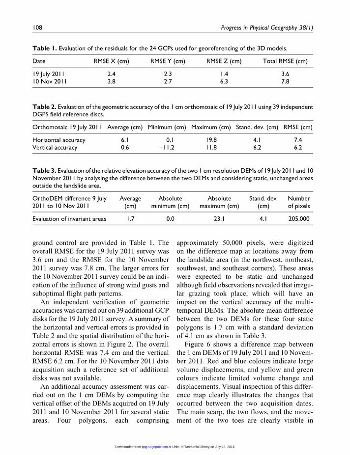
ground control are provided in Table 1. The

overall RMSE for the 19 July 2011 survey was

3.6 cm and the RMSE for the 10 November

2011 survey was 7.8 cm. The larger errors for

the 10 November 2011 survey could be an indi-

cation of the influence of strong wind gusts and

suboptimal flight path patterns.

An independent verification of geometric

accuracies was carried out on 39 additional GCP

disks for the 19 July 2011 survey. A summary of

the horizontal and vertical errors is provided in

Table 2 and the spatial distribution of the hori-

zontal errors is shown in Figure 2. The overall

horizontal RMSE was 7.4 cm and the vertical

RMSE 6.2 cm. For the 10 November 2011 data

acquisition such a reference set of additional

disks was not available.

An additional accuracy assessment was car-

ried out on the 1 cm DEMs by computing the

vertical offset of the DEMs acquired on 19 July

2011 and 10 November 2011 for several static

areas. Four polygons, each comprising

approximately 50,000 pixels, were digitized

on the difference map at locations away from

the landslide area (in the northwest, northeast,

southwest, and southeast corners). These areas

were expected to be static and unchanged

although field observations revealed that irregu-

lar grazing took place, which will have an

impact on the vertical accuracy of the multi-

temporal DEMs. The absolute mean difference

between the two DEMs for these four static

polygons is 1.7 cm with a standard deviation

of 4.1 cm as shown in Table 3.

Figure 6 shows a difference map between

the 1 cm DEMs of 19 July 2011 and 10 Novem-

ber 2011. Red and blue colours indicate large

volume displacements, and yellow and green

colours indicate limited volume change and

displacements. Visual inspection of this differ-

ence map clearly illustrates the changes that

occurred between the two acquisition dates.

The main scarp, the two flows, and the move-

ment of the two toes are clearly visible in

Table 1. Evaluation of the residuals for the 24 GCPs used for georeferencing of the 3D models.

Date RMSE X (cm) RMSE Y (cm) RMSE Z (cm) Total RMSE (cm)

19 July 2011 2.4 2.3 1.4 3.610 Nov 2011 3.8 2.7 6.3 7.8

Table 2. Evaluation of the geometric accuracy of the 1 cm orthomosaic of 19 July 2011 using 39 independentDGPS field reference discs.

Orthomosaic 19 July 2011 Average (cm) Minimum (cm) Maximum (cm) Stand. dev. (cm) RMSE (cm)

Horizontal accuracy 6.1 0.1 19.8 4.1 7.4Vertical accuracy 0.6 –11.2 11.8 6.2 6.2

Table 3. Evaluation of the relative elevation accuracy of the two 1 cm resolution DEMs of 19 July 2011 and 10November 2011 by analysing the difference between the two DEMs and considering static, unchanged areasoutside the landslide area.

OrthoDEM difference 9 July2011 to 10 Nov 2011

Average(cm)

Absoluteminimum (cm)

Absolutemaximum (cm)

Stand. dev.(cm)

Numberof pixels

Evaluation of invariant areas 1.7 0.0 23.1 4.1 205,000




the DEMs and difference image. Furthermore,

the difference image illustrates that material is

removed from the northern, central flank of the

landslide and has contributed to the movement

of the small toe. Figure 6 also illustrates the rel-

atively small vertical displacements of the

large toe (*0.5 m) and the general shape of

these movements as concentric half-circles.

The static oval shaped feature is also clearly

visible in this difference image.

3 Deformation computations usingCOSI-Corr

The relative displacements between two image

acquisition dates were computed using the

Figure 6. Difference between the 1 cm DEMs of 19 July 2011 and 10 November 2011 illustrating the surfacechanges and as such the dynamics of the landslide. Note the significant retreat of the main scarp and theexpansion of the toes.

Lucieer et al. 109



image correlation method implemented in the

COSI-Corr package. All images were resampled

to 10 cm resolution for better performance of

COSI-Corr. At the full resolution of 1 cm the fea-

tures between the images were too different for

reliable image correlation; hence a reduction in

resolution was required. The use of the shaded

relief map to compute displacements between

two image dates provided the best results and

was superior over all the other single-band

images. The statistical correlation method

yielded the best results compared with the

visual interpretation of the displacements on

the landslides. As described in section II.5, the

settings of window size, step size, and search

radius requires heuristic fine tuning and

some a priori knowledge of the deformations

derived, e.g. from visual interpretation of the

photographs or field observations. The best

parameter settings for the statistical correlator

for deformation mapping were a window size

of 64 pixels, a step size of 8 pixels and a search

radius of 50 pixels (5 m). Table 4 shows the

displacements (and standard deviations) of the

two toes of Home Hill landslide computed by

COSI-Corr for the two UAV survey dates.

Between brackets the average displacement

per day is presented. Table 4 provides an esti-

mate of the rate of displacement per day

but it should of course be noted that the displa-

cement often occurs stepwise in surges and that

the time between the different image acquisi-

tions dates does not allow a very detailed

assessment of the deformation velocity. It is

therefore only possible to present an average

deformation velocity per day.

Figure 7 shows the results of the image corre-

lation algorithm between 19 July 2011 and 10

November 2011 as vector fields plotted on a dis-

placements magnitude map. These results were

obtained using the shaded relief single images

of the two dates, the statistical correlator of

COSI-Corr, and a window size of 8–64 pixels

with a search radius of 5 m. The vector field

of Figure 7 is computed by combining the east–

west and north–south displacement. The white

vectors indicate the computed direction of move-

ment and the length of the vectors indicates the

relative displacement. The computed displace-

ments range from 0 to 6.9 m with a standard

deviation of 1.49 m. The figure clearly shows the

high dynamics of the small, northern toe (4–7 m)

and the slower but steady movement of the large,

southern toe (1–2 m). At the edges of the toes,

near the scarps and on the main body of the slide

the computed displacements show a less clear

image. The movements are more complex, edges

are steep and rotational movements probably

make it difficult for the image correlation algo-

rithm to produce reliable results. The static

oval-shaped block of 16�5 m in the southern part

of the main body of the slide is very well identi-

fied by the algorithm. The longitudinal displace-

ments for the central parts of the two toes are

accurately computed (based on visual validation

of clearly identifiable features). The lateral flow

of material at the end of the toes is also appropri-

ately represented. Displacements of vegetation

patches and chunks of ground material are cor-

rectly identified. At the active part of the scarp

the algorithm suggests a northwest movement,

however, the chunk of collapsed material

moves southeast in reality. Some vectors are

computed for the static grass area outside the

landslide area and so far no explanation for

these suggested movements was found.

Table 4. Displacements in metres of selected Home Hill landslide features computed using the algorithmCOSI-Corr (Leprince et al., 2007). Total displacements between image dates and their standard deviationare given. The average daily displacement between image acquisition dates is presented in brackets.

Image acquisition dates Large toe Small toe

19 July 2011 to 10 Nov 2011 (123 days) 127 cm + 14 (1.0 cm/day) 468 cm + 17 (3.8 cm/day)




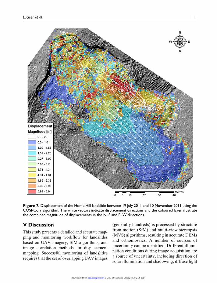
V Discussion

This study presents a detailed and accurate map-

ping and monitoring workflow for landslides

based on UAV imagery, SfM algorithms, and

image correlation methods for displacement

mapping. Successful monitoring of landslides

requires that the set of overlapping UAV images

(generally hundreds) is processed by structure

from motion (SfM) and multi-view stereopsis

(MVS) algorithms, resulting in accurate DEMs

and orthomosaics. A number of sources of

uncertainty can be identified. Different illumi-

nation conditions during image acquisition are

a source of uncertainty, including direction of

solar illumination and shadowing, diffuse light

Figure 7. Displacement of the Home Hill landslide between 19 July 2011 and 10 November 2011 using theCOSI-Corr algorithm. The white vectors indicate displacement directions and the coloured layer illustratethe combined magnitude of displacements in the N–S and E–W directions.

Lucieer et al. 111



under overcast conditions or direct sunlight

resulting in different image contrast. Weather

conditions with scattered clouds and resulting

sharp and dark shadows makes the process

even more difficult. Differences in illumina-

tion conditions in addition to differences in

vegetation condition (e.g. lush spring grass

versus short winter grass) between the acquisi-

tion dates can hamper the COSI-Corr algo-

rithm to identify matching features between

images acquired under different lighting con-

ditions. Since the algorithm searches for simi-

lar surface patterns in a specified search radius,

clouds and cloud shadows have an impact on

these patterns and hence an impact on the dis-

placement vector computation.

The evaluation of the obtained accuracy of

the orthomosaics and DEMs is not an easy task.

We recommend the use of two sets of clearly

visible reference markers (GCPs) randomly

placed on and around the landslide with accu-

rate XYZ coordinates measured by DGPS or

more accurate means (e.g. Totalstation). One

set of GCPs can then be used for the orthorec-

tification process and the second set is useful

for accuracy assessment. James and Robson

(2012) give a minimum relative precision ratio

of 1:1000 (coordinate precision: viewing dis-

tance) for SfM projects using Bundler and

PMVS2. For a flying height of *40 m AGL

this rule should result in a coordinate precision

of 4 cm. The RMSE values in Tables 1 and 2

show that our accuracy results are close, but

slightly worse, compared to this theoretical pre-

cision. Harwin and Lucieer (2012) achieved

absolute accuracies of 2.5–4 cm, however, their

study also included oblique UAV photography

and photography from lower flight runs.

The displacement algorithm uses pattern

matching on the surface of the landslide to

determine the direction and the size of the

movements. Input in this algorithm is a single

image band. From the various inputs we used,

the shaded relief map, derived from the DEM,

gave the best results. Shaded relief simulates the

relative shadowing on the topography based on

a solar azimuth of 315� and solar elevation of

45�. The reason that shaded relief is superior

over the other single-band images is probably

because shaded relief enhances the surface pat-

terns on the landslide. In future research we plan

to experiment with other DEM derivatives such

as slope and convexity, which are independent

of illumination settings. Herman et al. (2011)

used COSI-Corr to quantify the displacements

of glaciers and they found that the algorithm is

sensitive to the initial settings of window size,

step size, and search range. These a priori set-

tings will hamper a fully automated computa-

tion of displacement calculations.

The displacement algorithm proved to work

well as long as the displacements of the land-

slide are horizontal and the landslide surface

patterns remain at the surface during displace-

ment. As soon as rotational and revolving dis-

placements take place and surface features of

the landslide are buried, the surface patterns are

lost and COSI-Corr is unable to find correlated

surface patterns.

The image change analysis showed that the

period between 19 July 2011 and 10 November

2011 was an active period for landslide move-

ments. The triggering mechanism for the active

period was most likely the rainfall. The year

2011 was an exceptionally wet year with 950

mm of rainfall (station Kingston, Tasmania)

while the long-term (1882–2011) annual aver-

age is 616 mm (Bureau of Meteorology, Austra-

lian Government5). Furthermore, the volume of

rainfall in the month of April was extreme at

156.2 mm, while the monthly average is 51.4

mm. Two-thirds of this monthly value, i.e.

107.2 mm (Station Kingston, Tasmania), fell

on 13 April 2011 (Bureau of Meteorology, Aus-

tralian Government). The month of May 2011

was relatively dry (35 mm of rain) but another

76.5 mm of rain fell in just 36 hours on 8 and

9 June. These extreme rainfall events may have

reactivated the Home Hill landslide, however,

we did not obtain UAV imagery for the period




directly before and after these rainfall events to

prove this hypothesis.

VI Conclusions

In this study, we used a UAV platform equipped

with a standard digital camera and GPS to col-

lect multi-temporal sets of very high resolution

RGB images over the active Home Hill land-

slide in Tasmania. Structure from Motion (SfM)

and multi-view stereopsis (MVS) methods were

used to convert hundreds of overlapping images

into 3D point clouds, DEMs and orthomosaics at

1 cm resolution. The accuracy of the SfM tech-

nique was tested with 39 DGPS ground control

points resulting in a horizontal RMSE of 7.4

cm and a vertical RMSE of 6.2 cm. The multi-

date DEMs were converted into shaded relief

images and landslide dynamics detected using

an image correlation technique. The COSI-Corr

image correlation algorithm was applied to

compute the horizontal displacements of land-

slide features showing displacement magni-

tudes up to 7 m. These semi-automatically

mapped displacements were compared with

visual interpretation of displacements. The

algorithm successfully quantified movements

of chunks of ground material, patches of vege-

tation, and the toes of the landslide, but was

less successful in mapping the retreat of

the main scarp. Our results indicate that a

combination of UAV-based imagery and

SfM algorithms for 3D surface reconstruction

and subsequent image correlation on SfM

products, such as DEMs and orthophotos, can

be used for flexible and accurate monitoring

of landslides.

Acknowledgements

The team of Dr Leprince of the California Institute of

Technology (CalTech) is acknowledged for making

available their COSI-Corr package. We thank the

Home Hill vineyard for providing access to the land-

slide. We would also like to acknowledge the help of

students in the KGG375 GIS: Advanced Spatial

Analysis unit in semester two of 2011 with collecting

GPS ground control coordinates. Finally, we thank

the anonymous reviewers for their valuable sugges-

tions and comments.

Funding

The authors are grateful for the financial support

received from the Visiting Fellowship Program of

the University of Tasmania (UTAS).

Notes

1. See the official Mikrokopter open source quad-rotor

homepage, http://www.mikrokopter.com.

2. See ‘Image-based 3D modeling’, http://www.agisoft.ru.

3. See ENVI image processing software, http://www.exe-

lisvis.com.

4. See http://www.tectonics.caltech.edu/slip_history/spot_

coseis.

5. See http://www.bom.gov.au.

References

Abellan A, Calvet J, Vilaplana JM, et al. (2010) Detection

and spatial prediction of rockfalls by means of ter-

restrial laser scanner monitoring. Geomorphology

119: 162–171.

Abellan A, Jaboyedoff M, Oppikofer T, et al. (2009)

Detection of millimetric deformation using a terrestrial

laser scanner: Experiment and application to a rockfall

event. Natural Hazards and Earth System Science 9:

365–372.

Avelar AS, Coelho Netto AL, Lacerda WA, et al. (2013)

Mechanisms of the recent catastrophic landslides in

the mountainous range of Rio de Janeiro, Brazil. In:

Margottini C, Canuti P, and Sassa K (eds) Landslide

Science and Practice. Volume 4: Global Environmental

Change. Berlin: Springer, 265–270.

Ayoub F, LePrince S and Keene L (2009) User’s guide to

COSI-Corr: Co-registration of optically sensed images

and correlation. Available at: http://www.tectonics.cal-

tech.edu/slip_history/spot_coseis/pdf_files/cosi-corr_

guide.pdf.

Campbell NDF, Vogiatzis G, Hern C, et al. (2008) Using

multiple hypotheses to improve depth-maps for multi-

view stereo. In: Computer Vision – ECCV 2008, Part

I, Berlin: Springer, 766–779.

Carvajal F, Aguera F and Perez M (2011) Surveying a

landslide in a road embankment using unmanned aerial

vehicle photogrammetry. International Conference on

Unmanned Aerial Vehicle in Geomatics (UAV-g),

Lucieer et al. 113


http://www.tectonics.caltech.edu/slip_history/spot_coseis

http://www.tectonics.caltech.edu/slip_history/spot_coseis

http://www.tectonics.caltech.edu/slip_history/spot_coseis/pdf_files/cosi-corr_guide.pdf




14–16 September, Zurich. International Archives of the

Photogrammetry, Remote Sensing and Spatial Infor-

mation Sciences XXXVIII-1/C22: 201–206.

Dai FC, Xu C, Yao X, et al. (2011) Spatial distribution of

landslides triggered by the 2008 MS 8.0 Eenchuan

earthquake, China. Journal of Asian Earth Sciences 40:

883–895.

Delacourt C, Allemand P, Berthier E, et al. (2007) Remote-

sensing techniques for analysing landslide kinematics:

A review. Bulletin de la Societe Geologique de France

178: 89–100.

Dewitte O, Jasselette JC, Cornet Y, et al. (2008)

Tracking landslide displacements by multi-temporal

DTMs: A combined aerial stereophotogrammetric

and LiDAR approach in western Belgium. Engineer-

ing Geology 99: 11–22.

Dikau R, Brunsden D, Schrott L, et al. (1996) Landslide

Recognition. Chichester: Wiley.

d’Oleire-Oltmanns S, Marzolff I, Peter K, et al. (2012)

Unmanned aerial vehicle (UAV) for monitoring soil

erosion in Morocco. Remote Sensing 4: 3390–3416.

Doneus M, Verhoeven G, Fera M, et al. (2011) From

deposit to point cloud – a study of low-cost computer

vision approaches for the straightforward documenta-

tion of archaeological excavations. Geoinformatics 6:

81–88.

Dunford R, Michel K, Gagnage M, et al. (2009) Potential

and constraints of Unmanned Aerial Vehicle technol-

ogy for the characterization of Mediterranean riparian

forest. International Journal of Remote Sensing 30:

4915–4935.

Fiorucci F, Cardinali M, Carla R, et al. (2011) Seasonal

landslide mapping and estimation of landslide mobili-

zation rates using aerial and satellite images. Geo-

morphology 129: 59–70.

Fonstad MA, Dietrich JT, Courville BC, et al. (2013)

Topographic structure from motion: A new develop-

ment in photogrammetric measurement. Earth Surface

Processes and Landforms 38(4): 421–430.

Furukawa Y and Ponce J (2009) Accurate camera cali-

bration from multi-view stereo and bundle adjust-

ment. International Journal of Computer Vision 84:

257–268.

Furukawa Y and Ponce J (2010) Accurate, dense, and robust

multi-view stereopsis. IEEE Transactions on Pattern

Analysis and Machine Intelligence 32: 1362–1376.

Glenn NF, Streutker DR, Chadwick DJ, et al. (2006)

Analysis of LiDAR-derived topographic information

for characterizing and differentiating landslide mor-

phology and activity. Geomorphology 73: 131–148.

Gorum T, Fan X, Van Westen CJ, et al. (2011) Distribution

pattern of earthquake-induced landslides triggered by

the 12 May 2008 Wenchuan earthquake. Geomorphol-

ogy 133: 152–167.

Guzzetti F (2000) Landslide fatalities and the evaluation

of landslide risk in Italy. Engineering Geology 58:

89–107.

Guzzetti F, Mondini AC, Cardinali M, et al. (2012)

Landslide inventory maps: New tools for an old prob-

lem. Earth-Science Reviews 112: 42–66.

Harwin S and Lucieer A (2012) Assessing the accuracy of

georeferenced point clouds produced via multi-view

stereopsis from unmanned aerial vehicle (UAV) ima-

gery Remote Sensing 4: 1573–1599.

Herman F, Anderson B and LePrince S (2011) Mountain

glacier velocity variation during a retreat/advance

cycle quantified using sub-pixel analysis of ASTER

images. Journal of Glaciology 57: 197–207.

James MR and Robson S (2012) Straightforward recon-

struction of 3d surfaces and topography with a camera:

Accuracy and geoscience application. Journal of

Geophysical Research 117: F03017.

Joyce KE, Belliss SE, Samsonov SV, et al. (2009) A review

of the status of satellite remote sensing and image pro-

cessing techniques for mapping natural hazards and

disasters. Progress in Physical Geography 33: 83–207.

Kelcey J and Lucieer A (2012) Sensor correction of a 6-

band multispectral imaging sensor for UAV remote

sensing. Remote Sensing 4: 1462–1493.

Laliberte AS and Rango A (2009) Texture and scale in

object-based analysis of subdecimeter resolution

unmanned aerial vehicle (UAV) imagery. IEEE

Transactions on Geoscience and Remote Sensing 47:

1–10.

Laliberte AS, Goforth MA, Steele CM, et al. (2011)

Multispectral remote sensing from unmanned aircraft:

Image processing workflows and applications for ran-

geland environments. Remote Sensing 3: 2529–2551.

Laliberte AS, Herrick JE, Rango A, et al. (2010) Acqui-

sition, orthorectification, and object-based classifica-

tion of Unmanned Aerial Vehicle (UAV) imagery for

rangeland monitoring. Photogrammetric Engineering

and Remote Sensing 76: 661–672.

Leprince S, Barbot S, Ayoub F, et al. (2007) Automatic

and precise orthorectification, co-registration, and sub-

pixel correlation of satellite images, application to




ground deformation measurements. IEEE Transactions

on Geoscience and Remote Sensing 46: 1529–1558.

Leprince S, Berthier E, Ayoub F, et al. (2008) Monitoring

earth surface dynamics with optical imagery. EOS,

Transactions American Geophysical Union 89: 1–2.

Lowe D (2004) Distinctive image features from scale-

invariant key points. International Journal of Com-

puter Vision 60: 91–110.

Lucieer A, Turner D, King DH, et al. (2014) Using an

Unmanned Aerial Vehicle (UAV) to capture micro-

topography of Antarctic moss beds. International Jour-

nal of Applied Earth Observation and Geoinformation.

27(Part A): 53–62.

McIntosh PD, Price DM, Eberhard R, et al. (2009) Late

Quaternary erosion events in lowland and mid-altitude

Tasmania in relation to climate change and first human

arrival. Quaternary Science Reviews 28: 850–872.

McKean J and Roering J (2004) Objective landslide

detection and surface morphology mapping using high-

resolution airborne laser altimetry. Geomorphology 57:

331–351.

Metternicht G, Hurni L and Gogu R (2005) Remote sen-

sing of landslides: An analysis of the potential contri-

bution to geo-spatial systems for hazard assessment in

mountainous environments. Remote Sensing of Envi-

ronment 98: 284–303.

Nadim F, Kjekstad O, Peduzzi P, et al. (2006) Global

landslide and avalanche hotspots. Landslides 3:

159–173.

Neitzel F and Klonowski J (2011) Mobile 3D mapping

with a low-cost UAV system. International Conference

on Unmanned Aerial Vehicle in Geomatics (UAV-g),

14–16 September, Zurich. International Archives of the

Photogrammetry, Remote Sensing and Spatial Infor-

mation Sciences XXXVIII-1/C22: 39–44.

Niethammer U, James MR, Rothmund S, et al. (2012)

UAV-based remote sensing of the Super-Sauze land-

slide: Evaluation and results. Engineering Geology

128: 2–11.

Niethammer U, Rothmund S, James MR, et al. (2010)

UAV-based remote sensing of landslides. ISPRS Com-

mission V Mid-Term Symposium ‘Close Range Image

Measurement Techniques’, ‘21–24 June, ‘Newcastle

upon Tyne. International Archives of the Photogramme-

try, Remote Sensing and Spatial Information Sciences

XXXVIII, Part 5: 496–501.

Razak KA, Straatsma MW, van Westen CJ, et al. (2011)

Airborne laser scanning of forested landslides

characterization: Terrain model quality and visualiza-

tion. Geomorphology 126: 186–200.

Scherler D, Leprince S and Strecker MR (2008) Glacier-

surface velocities in alpine terrain from optical satel-

lite imagery: Accuracy improvement and quality

assessment. Remote Sensing of Environment 112:

3806–3819.

Schuster RL and Fleming WF (1986) Economic losses and

fatalities due to landslides. Bulletin of the Association

of Engineering Geologists 23: 11–28.

Snavely N, Seitz SM and Szeliski R (2008) Modeling the

world from internet photo collections. International

Journal of Computer Vision 80: 189–210.

Swiss Re (2011a) Flood risk on the rise in Brazil.

Available at: http://www.swissre.com/rethinking/cli-

mate_and_natural_disaster_risk/Flood_risk_on_the_

rise_in_Brazil.html.

Swiss Re (2011b) Natural catastrophes and man-made

disasters in 2010. Sigma 1/2011. Available at:

http:// media.swissre.com/documents/sigma1_2011_

en.pdf.

Travelletti J, Delacourt C, Allemand P, et al. (2012) Cor-

relation of multi-temporal ground-based optical images

for landslide monitoring: Application, potential and

limitations. ISPRS Journal of Photogrammetry and

Remote Sensing 70: 39–55.

Triggs B, McLauchlan P, Hartley R, et al. (2000) Bundle

adjustment: A modern synthesis. In: Triggs B, Zisser-

man A and Szeliski R (eds) Vision Algorithms: Theory

and Practice. Berlin: Springer, 298–372.

Turner D, Lucieer A and Watson C (2012) An automated

technique for generating georectified mosaics from

ultra-high resolution Unmanned Aerial Vehicle (UAV)

imagery, based on Structure from Motion (SfM) point

clouds. Remote Sensing 4: 1392–1410.

van Westen CJ, Castellanos E and Kuriakose SL (2008)

Spatial data for landslide susceptibility, hazard, and

vulnerability assessment: An overview. Engineering

Geology 102: 112–131.

Varnes DJ and International Association of Engineering

Geology (IAEG) (1984) Landslide Hazard Zonation:

A Review of Principles and Practice. Paris:

UNESCO.

Ventura G, Vilardo G, Terranova C, et al. (2011) Tracking

and evolution of complex active landslides by multi-

temporal airborne LiDAR data: The Montaguto land-

slide (southern Italy). Remote Sensing of Environment

115: 3237–3248.

Lucieer et al. 115


http://www.swissre.com/rethinking/climate_and_natural_disaster_risk/Flood_risk_on_the_rise_in_Brazil.html



http://media.swissre.com/documents/sigma1_2011_en.pdf





Verhoeven G (2011) Taking computer vision aloft –

archaeological three-dimensional reconstructions from

aerial photographs with photoscan. Archaeological

Prospection 18: 67–73.

Westoby M, Brasington J, Glasser N, et al. (2012) ‘struc-

ture-from-motion’ photogrammetry: A low-cost, effec-

tive tool for geoscience applications. Geomorphology

179: 300–314.

Zarco-Tejada PJ, Gonzalez-Dugo V and Berni JAJ (2011)

Fluorescence, temperature and narrow-band indices

acquired from a UAV platform for water stress detec-

tion using a micro-hyperspectral imager and a thermal

camera. Remote Sensing of Environment 117: 322–337.

Zillman J (1999) The physical impact of disaster. In:

Ingleton J (ed.) Natural Disaster Management.

Leicester: Tudor Rose Holdings Ltd.




Documents

PPG515293 97. - Arko Lucieer - Remote Sensing Scientistlucieer.net/wp-content/uploads/2014/11/2014_Lucieer_PPG_HomeHill.pdf · human casualties and economic losses, largely as damage