Predicting Accident Rates From General Aviation Pilot Total Flight Hours

William R. KnechtCivil Aerospace Medical Institute,Federal Aviation Administration Oklahoma City, OK 73125

February 2015

Final Report

DOT/FAA/AM-15/3Office of Aerospace MedicineWashington, DC 20591

Federal AviationAdministration

NOTICE

This document is disseminated under the sponsorship of the U.S. Department of Transportation in the interest

of information exchange. The United States Government assumes no liability for the contents thereof.

___________

This publication and all Office of Aerospace Medicine technical reports are available in full-text from the

Federal Aviation Administration website.

i

Technical Report Documentation Page

1. Report No. 2. Government Accession No. 3. Recipient's Catalog No.

DOT/FAA/AM-15/3 4. Title and Subtitle 5. Report Date

Predicting Accident Rates From General Aviation Pilot Total Flight Hours

February 2015 6. Performing Organization Code

7. Author(s) 8. Performing Organization Report No. Knecht WR

9. Performing Organization Name and Address 10. Work Unit No. (TRAIS) FAA Civil Aerospace Medical Institute P.O. Box 25082 11. Contract or Grant No. Oklahoma City, OK 73125 12. Sponsoring Agency name and Address 13. Type of Report and Period Covered Office of Aerospace Medicine Federal Aviation Administration 800 Independence Ave., S.W. Washington, DC 20591

14. Sponsoring Agency Code

15. Supplemental Notes Work was accomplished under approved task AHRR521 16. Abstract In his 2001 book, The Killing Zone, Paul Craig presented evidence that general aviation (GA) pilot fatalities are related to relative flight experience (total flight hours, or TFH). We therefore ask if there is a range of TFH over which GA pilots are at greatest risk? More broadly, can we predict pilot accident rates, given TFH? Many researchers implicitly assume that GA accident rates are a linear function of TFH when, in fact, that relation appears nonlinear. This work explores the ability of a nonlinear gamma-based modeling function to predict GA accident rates from noisy TFH data (random sampling errors). Two sets of National Transportation Safety Board /Federal Aviation Administration (FAA) data, parsed by pilot instrument rating, produced weighted goodness-of-fit estimates of .654 and .775 for non-instrument-rated and instrument-rated pilots, respectively. This model class would be useful in direct prediction of GA accident rates and as a statistical covariate to factor in flight risk during other types of modeling. Applied to FAA data, these models show that the range for relatively high risk may be far broader than first imagined, and may extend well beyond the 2,000-hour mark before leveling off to a baseline rate.

17. Key Words 18. Distribution Statement

General Aviation, Accidents, Accident Rates,Flight Hours, Modeling, Predicting

Document is available to the public through the Internet:

http://www.faa.gov/go/oamtechreports/

19. Security Classif. (of this report) 20. Security Classif. (of this page) 21. No. of Pages 22. Price

Unclassified Unclassified 14 Form DOT F 1700.7 (8-72) Reproduction of completed page authorized

iii

ACKNOWLEDGMENTS

Deep appreciation is extended to Joe Mooney, FAA (AVP-210), for his help reviewing the NTSB database queries that provided the accident data used here, to David Nelms, FAA (AAM-300), for providing TFH from the DIWS database, and to Dana Broach, FAA (AAM-500) for valuable commentary on this series of manuscripts.

This research was conducted under the Flight Deck Program Directive/Level of Effort Agreement between FAA Headquarters and the Aerospace Human Factors Division of the Civil Aerospace Medical Institute, sponsored by the Office of Aerospace Medicine and supported through the FAA NextGen Human Factors Division.

v

Contents

Predicting Accident Rates From General Aviation Pilot Total Flight Hours

INTRODUCTION . . . . . . . . . . . . . . . . . . . . . . . . . . . . . . . . . . . . . . . . . . . . . . . . . . . . . . . . . . . . . . . 1 The Problem With Rates . . . . . . . . . . . . . . . . . . . . . . . . . . . . . . . . . . . . . . . . . . . . . . . . . . . . . . . 2METHOD . . . . . . . . . . . . . . . . . . . . . . . . . . . . . . . . . . . . . . . . . . . . . . . . . . . . . . . . . . . . . . . . . . . . . 2 The Modeling Function . . . . . . . . . . . . . . . . . . . . . . . . . . . . . . . . . . . . . . . . . . . . . . . . . . . . . . . 2 The Empirical Data . . . . . . . . . . . . . . . . . . . . . . . . . . . . . . . . . . . . . . . . . . . . . . . . . . . . . . . . . . . 3 Important Considerations . . . . . . . . . . . . . . . . . . . . . . . . . . . . . . . . . . . . . . . . . . . . . . . . . . . . . . 3 Parameter Estimation . . . . . . . . . . . . . . . . . . . . . . . . . . . . . . . . . . . . . . . . . . . . . . . . . . . . . . . . . 4 The Problem of Noise . . . . . . . . . . . . . . . . . . . . . . . . . . . . . . . . . . . . . . . . . . . . . . . . . . . . . . . . . 4 Parameter Start Values and Evolution . . . . . . . . . . . . . . . . . . . . . . . . . . . . . . . . . . . . . . . . . . . . . 5RESULTS . . . . . . . . . . . . . . . . . . . . . . . . . . . . . . . . . . . . . . . . . . . . . . . . . . . . . . . . . . . . . . . . . . . . . . 5 Modeling the Accident Rate Histograms . . . . . . . . . . . . . . . . . . . . . . . . . . . . . . . . . . . . . . . . . . . 5 Model Evaluation . . . . . . . . . . . . . . . . . . . . . . . . . . . . . . . . . . . . . . . . . . . . . . . . . . . . . . . . . . . . 6 USING Grate . . . . . . . . . . . . . . . . . . . . . . . . . . . . . . . . . . . . . . . . . . . . . . . . . . . . . . . . . . . . . . . . 6 A Point-Estimate of GA Flight Risk . . . . . . . . . . . . . . . . . . . . . . . . . . . . . . . . . . . . . . . . . . . . . . 6 A Cumulative Estimate of GA Flight Risk . . . . . . . . . . . . . . . . . . . . . . . . . . . . . . . . . . . . . . . . . . 7DISCUSSION . . . . . . . . . . . . . . . . . . . . . . . . . . . . . . . . . . . . . . . . . . . . . . . . . . . . . . . . . . . . . . . . . . . 7REFERENCES . . . . . . . . . . . . . . . . . . . . . . . . . . . . . . . . . . . . . . . . . . . . . . . . . . . . . . . . . . . . . . . . . . 8

1

Predicting Accident rAtes From generAl AviAtion Pilot totAl Flight hours

Is there a range of pilot flight hours over which general aviation (GA) pilots are at greatest risk? More broadly, can we predict accident rates, given a pilot’s total flight hours (TFH)? Many GA research studies implicitly assume that accident rates are a linear function of TFH when, in fact, that relation appears nonlinear. This work explores the ability of a nonlinear gamma-based function (Grate) to predict GA accident rates from noisy TFH data. Two sets of National Transportation Safety Board (NTSB)/Federal Aviation Administration (FAA) data, parsed by pilot instrument rating, produced weighted goodness-of-fit (R2

w) estimates of .654 and .775 for non-instrument-rated (non-IR) and instrument-rated pilots (IR), respectively. This model class would be useful in direct prediction of GA accident rates, and as a statistical covariate to factor in flight risk during other types of modeling. Applied to FAA data, these models show that the range for relatively high risk may be far broader than first imagined, and may extend well beyond the 2,000-hour mark before leveling off to a baseline rate.

INTRODUCTION

Total flight hours has long been considered one of the risk fac-tors in aviation, and is often used to represent either pilot flight experience or cumulative risk exposure (e.g., Dionne, Gagné & Vanasse, 1992; Guohua, Baker, Grabowski, Qiang, McCarthy & Rebok, 2011; Mills, 2005; Sherman, 1997). TFH has served as both an independent variable in its own right, as well as a statistical covariate, to control for the effects of experience or risk.

Investigators have often unwittingly assumed a linear rela-tion between TFH and accident frequency and/or rate, that is, a straight-line prediction function ŷ=a+bx, with a as y-intercept and b as slope. However, evidence is emerging that such relations are actually nonlinear. For instance, Bazargan & Guzhva (2007) reported that the logarithmic transform log(TFH) significantly predicted GA fatalities in a logistic regression model. More recently, Knecht & Smith (2012) reported that a risk covariate starting with log(TFH), followed by a gamma transform, signifi-cantly predicted GA fatalities in a log-linear model.

In his 2001 book, The Killing Zone, Paul Craig presented early evidence that GA pilot fatalities might relate nonlinearly to TFH. Craig showed that fatalities occur most frequently at a middle range of TFH (≈50-350), and hypothesized that this band of time may be one in which pilots are at greatest risk due to overconfidence at having mastered flying the aircraft, combined with lack of actual experience and skill in dealing with rare, chal-lenging events. He supported this hypothesis with histograms of GA accident frequencies, although not with a formal model. In group after group, a similar pattern emerged in his data, one of a “skewed camel hump” with a long tail at higher TFH.

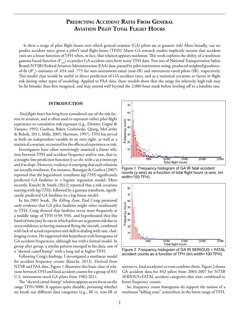
Following Craig’s findings, I investigated a nonlinear model for accident frequency counts (Knecht, 2012). Derived from NTSB and FAA data, Figure 1 illustrates this basic class of rela-tions between TFH and fatal accident counts for a group of 831 U.S. instrument-rated GA pilots from 1983-2011.

The “skewed camel-hump” relation appears as we focus on the range TFH<5000. It appears quite durable, persisting whether we break out different data categories (e.g., IR vs. non-IR or

serious vs. fatal accidents) or even combine them. Figure 2 shows GA accident data for 832 pilots from 2003-2007 for NTSB SERIOUS+FATAL accident categories that were combined to boost frequency counts.

So, frequency count histograms do support the notion of a nonlinear “killing zone” somewhere in the lower range of TFH.

Figure 1. Frequency histogram of GA IR fatal accident counts (y-axis) as a function of total flight hours (x-axis, bin width=100 TFH).

Figure 2. Frequency histogram of GA IR SERIOUS + FATAL accident counts as a function of TFH (bin width=100 TFH).

2

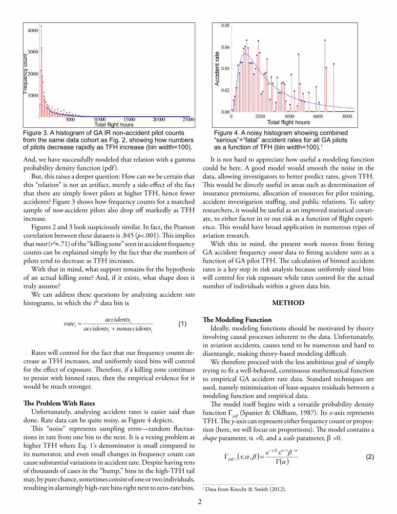
And, we have successfully modeled that relation with a gamma probability density function (pdf ).

But, this raises a deeper question: How can we be certain that this “relation” is not an artifact, merely a side-effect of the fact that there are simply fewer pilots at higher TFH, hence fewer accidents? Figure 3 shows how frequency counts for a matched sample of non-accident pilots also drop off markedly as TFH increase.

Figures 2 and 3 look suspiciously similar. In fact, the Pearson correlation between these datasets is .845 (p<.001). This implies that most (r2≈.71) of the “killing zone” seen in accident frequency counts can be explained simply by the fact that the numbers of pilots tend to decrease as TFH increases.

With that in mind, what support remains for the hypothesis of an actual killing zone? And, if it exists, what shape does it truly assume?

We can address these questions by analyzing accident rate histograms, in which the ith data bin is

It is not hard to appreciate how useful a modeling function could be here. A good model would smooth the noise in the data, allowing investigators to better predict rates, given TFH. This would be directly useful in areas such as determination of insurance premiums, allocation of resources for pilot training, accident investigation staffing, and public relations. To safety researchers, it would be useful as an improved statistical covari-ate, to either factor in or out risk as a function of flight experi-ence. This would have broad application in numerous types of aviation research.

With this in mind, the present work moves from fitting GA accident frequency count data to fitting accident rates as a function of GA pilot TFH. The calculation of binned accident rates is a key step in risk analysis because uniformly sized bins will control for risk exposure while rates control for the actual number of individuals within a given data bin.

METHOD

The Modeling FunctionIdeally, modeling functions should be motivated by theory

involving causal processes inherent to the data. Unfortunately, in aviation accidents, causes tend to be numerous and hard to disentangle, making theory-based modeling difficult.

We therefore proceed with the less ambitious goal of simply trying to fit a well-behaved, continuous mathematical function to empirical GA accident rate data. Standard techniques are used, namely minimization of least-squares residuals between a modeling function and empirical data.

The model itself begins with a versatile probability density function Gpdf (Spanier & Oldham, 1987). Its x-axis represents TFH. The y-axis can represent either frequency count or propor-tion (here, we will focus on proportions). The model contains a shape parameter, α >0, and a scale parameter, β >0.

Figure 3. A histogram of GA IR non-accident pilot counts from the same data cohort as Fig. 2, showing how numbers of pilots decrease rapidly as TFH increase (bin width=100).

Figure 4. A noisy histogram showing combined “serious”+“fatal” accident rates for all GA pilots as a function of TFH (bin width=100).1

ii

ii tsnonaccidenaccidents

accidentsrate+

= (1)

Rates will control for the fact that our frequency counts de-crease as TFH increases, and uniformly sized bins will control for the effect of exposure. Therefore, if a killing zone continues to persist with binned rates, then the empirical evidence for it would be much stronger.

The Problem With RatesUnfortunately, analyzing accident rates is easier said than

done. Rate data can be quite noisy, as Figure 4 depicts. This “noise” represents sampling error—random fluctua-

tions in rate from one bin to the next. It is a vexing problem at higher TFH where Eq. 1’s denominator is small compared to its numerator, and even small changes in frequency count can cause substantial variations in accident rate. Despite having tens of thousands of cases in the “hump,” bins in the high-TFH tail may, by pure chance, sometimes consist of one or two individuals, resulting in alarmingly high-rate bins right next to zero-rate bins. 1 Data from Knecht & Smith (2012).

( ) ( )αββα

ααβ

Γ=Γ

−−− 1

. ,; xexx

cpdf (2)

3

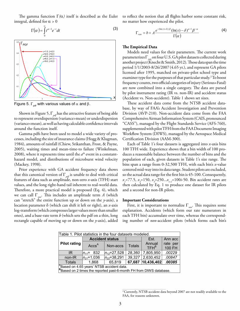
The gamma function G(α) itself is described as the Euler integral, defined for α > 0

Shown in Figure 5, Gpdf has the attractive feature of being able to represent overdispersion (variance>mean) or underdispersion (variance<mean), as well as having calculable confidence intervals around the function itself.

Gamma pdfs have been used to model a wide variety of pro-cesses, including the size of insurance claims (Hogg & Klugman, 1984), amounts of rainfall (Chiew, Srikanthan, Frost, & Payne, 2005), waiting times and mean-time-to failure (Winkelman, 2008), where it represents time until the ath event in a constant-hazard model, and distributions of microburst wind velocity (Mackey, 1998).

Prior experience with GA accident frequency data shows that this canonical version of Gpdf is unable to deal with critical features of data such as amplitude, non-zero x-axis (TFH) start values, and the long right-hand tail inherent to real-world data. Therefore, a more practical model is proposed (Eq. 4), which we can call Grate. This includes an amplitude term A (which can “stretch” the entire function up or down on the y-axis), a location parameter δ (which can shift it left or right), an x-axis log-transform (which compresses larger values more than smaller ones), and a base-rate term b (which sets the pdf on a thin, long rectangle capable of moving up or down on the y-axis), added

to reflect the notion that all flights harbor some constant risk, no matter how experienced the pilot.

The Empirical DataModels need values for their parameters. The current work

parameterizes Grate on four U.S. GA pilot datasets collected during another project (Knecht & Smith, 2012). Those data span the time period 1/1/2003-8/26/2007 (4.65 yr.), and represent GA pilots licensed after 1995, matched on private-pilot school type and examiner type for the purposes of that particular study.2 To boost frequency counts, two official categories of injury (Serious+Fatal) are now combined into a single category. The data are parsed by pilot instrument rating (IR vs. non-IR) and accident status (Accident vs. Non-accident). Table 1 shows set sizes.

These accident data come from the NTSB accident data-base, by way of FAA’s Accident Investigation and Prevention Division (AVP-210). Non-accident data come from the FAA Comprehensive Airman Information System (CAIS, pronounced “CASS”), managed by the Flight Standards Service (AFS-760), supplemented with pilot TFH from the FAA Document Imaging Workflow System (DIWS), managed by the Aerospace Medical Certification Division (AAM-300).

Each of Table 1’s four datasets is aggregated into x-axis bins 100 TFH wide. Experience shows that a bin width of 100 pro-duces a reasonable balance between the number of bins and the population of each, given datasets in Table 1’s size range. The bins span a range from 0-32,500 TFH, with each bin’s x-value centered mid-way into its data range. Student pilots are excluded, so the actual data range for the first bin is 45-100. Consequently, x1=77.5, x2=150, x3=250...xi>1=100i-50. Bin accident rates are then calculated by Eq. 1 to produce one dataset for IR pilots and a second for non-IR pilots.

Important ConsiderationsFirst, it is important to normalize Grate. This requires some

explanation. Accidents (which form our rate numerators in each TFH bin) accumulate over time, whereas the correspond-ing number of non-accident pilots (which forms each bin’s

2 Currently, NTSB accident data beyond 2007 are not readily available to the FAA, for reasons unknown.

( ) dtet t∫∞

−−=Γ0

1αα (3)

( )αβδ ααβδ

Γ−

+=Γ−−−− 1))(ln( ))(ln(xeAb

x

rate(4)

Figure 5. Gpdf with various values of α and β.

Table 1. Pilot statistics in the four datasets modeled.

Pilot rating Accident status Est.

Annual TFHB

Ann acc rate per 100 FH AccsA Non-accs Totals

IR n11= 832 n12=27,528 28,360 7,805,950 .00229 non-IR n21=1,036 n22=38,291 39,327 2,630,452 .00847 Totals 1,868 65,819 67,687 10,436,402 .00385

ABased on 4.65 years’ NTSB accident data. BBased on 2 times the reported past-6-month FH from DIWS database.

4

denominator) is based on a “snapshot” in time and is therefore considered a constant. Consequently, we should normalize our bin accident rates to reflect a standard unit time such as one year. In that event, each bin’s initial rate should be divided by the number of years over which accident data were accumulated (here, 4.65 years) to represent estimated accident rate per year, a.k.a. annualized rate.

Second, we need to clearly understand that, unlike accident frequency histograms, a distribution of rates is not technically a pdf, even though we may try to curve-fit binned rate data with a pdf-like function (e.g., Eq. 4).3 More specifically, to cumulate accident frequencies over a range of TFH, we would compute a pdf ’s definite integral over that range. In contrast, to cumulate the probability of having an accident over a range of TFH requires a different method (described later in Eq. 12).

Parameter EstimationThe NonlinearModelFit function of Mathematica 7.0 (Wol-

fram, 2008) is used to estimate parameters for Eq. 4. For unconstrained parameters, NonlinearModelFit offers a range of standard numerical methods (e.g., Newton-Gauss, quasi-Newton, Levenberg-Marquardt). For constrained parameters (the method used here), where starting and/or final parameter values are forced to lie within some range pmin<pt<pmax, the Karush-Kuhn-Tucker (KKT) method was used.

The Problem of NoiseNoisy data such as Figure 4’s pose great difficulty for standard

least-squares minimization. Parameters often fail to converge in rugged ratescapes, or may converge to a local minimum rather than a global one.

To confront the noise, we first tried the simplest approach of using wider data bins. Surprisingly, this had almost no effect. Accidents within these particular data tended to bunch up in several adjacent bins, leaving no way to smooth them without resorting to arbitrary “bin widths of convenience,” which would negate our attempt to standardize risk exposure by having equal bin widths.

We next tried another standard tactic, namely dropping outliers. Outliers can be defined in various ways, but a rule of thumb is to drop all data points (here, rates) greater than 2.5-3 standard deviations (s) from the group sample mean ȳ

This method was tested but abandoned for several reasons. Not only was it based on an (here invalid) assumption of distri-butional normality, but useful information was destroyed, and the extremely long tail of the fitting function resulted in an s so small that we end up dropping very few of the obviously noisy values in the tail that threatened our curve-fit.

A third standard approach was next tried, involving data-smoothing using moving averages. Unfortunately, this also had the effect of destroying information by smearing, greatly altering the “camel hump” representing the majority of the data.

A fourth approach was then considered. Simulated annealing (Kirkpatrick, Gelatt, & Vecchi, 1983) would involve adding noise to each parameter’s starting value before engaging in the gradient-descent, residual error-minimization process. Then, as that process progressed, we would “cool the noise,” allowing parameter estimates to bounce around and out of local minima until a global near-minimum could be found.

Nonetheless, in the case of noisy rate data, even such an elegant approach unfortunately would still leave us one major logical problem: All our data bins—including the noisy—would have equal opportunity to influence the residual sum-of-squares during the data-fit. Any “one bin, one vote” approach would implicitly allow all bins equal influence, no matter how many individuals each bin represented or what that bin’s expected variance was. This would confer inordinately large influence to sparsely populated bins, as well as to larger bins having inher-ently low reliability.

After being frustrated by the problems outlined above, we finally settled on the standard procedure of weighting empty bins by 0 while weighting non-empty bin’s accident rate ri by the inverse of its sample variance (1/si

2). This is easily done in Mathematica by supplying a vector Weights→w to Nonlinear-ModelFit, where w={w1, w2 ... wi}.

Since our data are rates are proportions, 0≤ri≤1, the ith bin weight wi becomes

ni being the ith bin’s total frequency count (accidents+non-accidents) used to derive ri, and Ni being the number of pilots in the general population with that range of TFH.

In this particular instance, we do not know Ni, so we shall assume a constant sample ratio ni/Ni, making the term 1-(ni/Ni) constant for all bins. Since weights only need to be expressed relative to each other during curve-fitting, we can eliminate this constant term, leading to a functional weight of

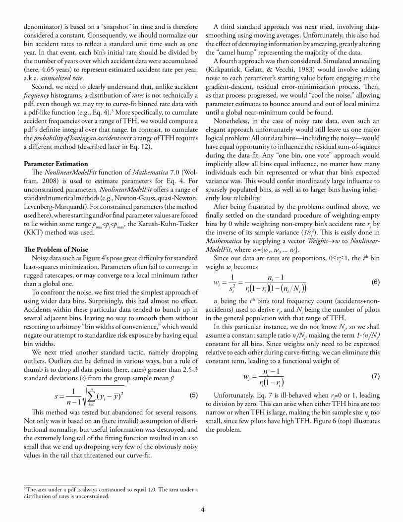
Unfortunately, Eq. 7 is ill-behaved when ri=0 or 1, leading to division by zero. This can arise when either TFH bins are too narrow or when TFH is large, making the bin sample size ni too small, since few pilots have high TFH. Figure 6 (top) illustrates the problem.

∑=

−−

=n

ii yy

ns

1

2)(1

1 (5)

3 The area under a pdf is always constrained to equal 1.0. The area under a distribution of rates is unconstrained.

( )ii

ii rr

nw−−

=1

1 (7)

( ) ( )( )iiii

i

ii Nnrr

ns

w−−−

==11

112

(6)

5

To address this issue, Eq. 7 is modified slightly by adding a term ε designed to constrain behavior at 0 and 1:

As Figure 6 shows, when ε is small, Eq. 8 closely approximates Eq. 7 over most of its range but self-limits gracefully at ri=0 and 1.

Parameter Start Values and EvolutionIn multidimensional parameter spaces with unknown local

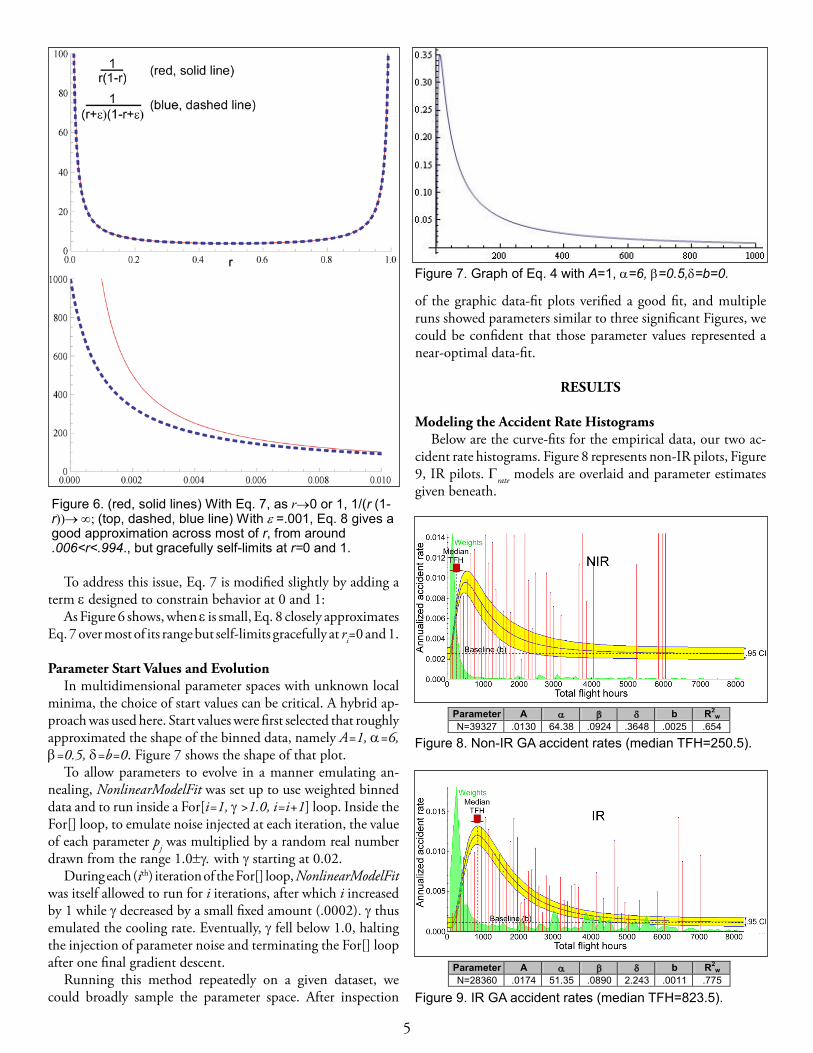
minima, the choice of start values can be critical. A hybrid ap-proach was used here. Start values were first selected that roughly approximated the shape of the binned data, namely A=1, α=6, β=0.5, δ=b=0. Figure 7 shows the shape of that plot.

To allow parameters to evolve in a manner emulating an-nealing, NonlinearModelFit was set up to use weighted binned data and to run inside a For[i=1, γ >1.0, i=i+1] loop. Inside the For[] loop, to emulate noise injected at each iteration, the value of each parameter pj was multiplied by a random real number drawn from the range 1.0±γ. with γ starting at 0.02.

During each (ith) iteration of the For[] loop, NonlinearModelFit was itself allowed to run for i iterations, after which i increased by 1 while γ decreased by a small fixed amount (.0002). γ thus emulated the cooling rate. Eventually, γ fell below 1.0, halting the injection of parameter noise and terminating the For[] loop after one final gradient descent.

Running this method repeatedly on a given dataset, we could broadly sample the parameter space. After inspection

of the graphic data-fit plots verified a good fit, and multiple runs showed parameters similar to three significant Figures, we could be confident that those parameter values represented a near-optimal data-fit.

RESULTS

Modeling the Accident Rate HistogramsBelow are the curve-fits for the empirical data, our two ac-

cident rate histograms. Figure 8 represents non-IR pilots, Figure 9, IR pilots. Grate models are overlaid and parameter estimates given beneath.

Figure 6. (red, solid lines) With Eq. 7, as r→0 or 1, 1/(r (1-r))→ ∞; (top, dashed, blue line) With ε =.001, Eq. 8 gives a good approximation across most of r, from around .006<r<.994., but gracefully self-limits at r=0 and 1.

Figure 7. Graph of Eq. 4 with A=1, α=6, β=0.5,δ=b=0.

Figure 8. Non-IR GA accident rates (median TFH=250.5).

Figure 9. IR GA accident rates (median TFH=823.5).

Parameter A α β δ b R2w

N=39327 .0130 64.38 .0924 .3648 .0025 .654

Parameter A α β δ b R2w

N=28360 .0174 51.35 .0890 2.243 .0011 .775

6

Each Figure shows accident rate (y-axis) plotted by TFH-of-pilot-at-the-time-of-accident (x-axis, bin width = 100). Each bin’s raw number of accidents (based on 4.65 years’ data) was divided by the total number of pilots (accident+non-accident) in the same range of TFH to produce a bin rate for that 100-hr range.4 The resulting rates were then divided by 4.65 to represent one average year’s rates before starting the curve-fitting process. Keep in mind that the height of the y-axis represents the prob-ability of having an accident over a 100-FH span, x±50.Grate is based on Eq. 4 with data weighted by Eq. 8 (ε =.001).

Relative weights are drawn in green and have been scaled to fit within the Figure. Empty bins (ni=0) were weighted 0 to prevent them from influencing the curve-fit. The yellow band surround-ing Grate represents its 95% confidence interval (CI).

Model EvaluationA model’s ability to predict empirical data can be expressed by

a variety of metrics. One of the simplest measures of goodness-of-fit is the coefficient of determination, R2. R2 varies between 0 and 1 and estimates the proportion of explained variance. The weighted form of R2 is nominally

with weighted means, for instance ȳw, of the form

However, Eq. 9 can throw values < 0 with nonlinear data, so we opt for the robust form of R2

w= r2w, the square of the weighted

correlation coefficient

With these data, Eq. 11 yields r2w-non-IR = .654 and r2

w-IR = .775, both in the “moderate” range of fit. This is surprisingly high, given the noisy data. The explanation is straightforward. We see from the distribution of weights and the .95CIs that these relatively high r2

w values are due to the weighting function (Eq. 8) assigning large weights mostly to low values of TFH. The large majority of pilots have low TFH (median values x˜NIR =250.5, x˜IR=823.5). Large ns increase the numerator of Eq. 8, thus bin weight. In practical terms, weights are simply reliability estimates that are higher when based on larger numbers coupled with proportions close to 0 or 1. The .95CI reflects this. As weights shrink, .95CI widens.

The downside of high reliability at low TFH is lower reliability at high TFH. Figures 8 and 9 show the penalty imposed by rate noise. We can predict fairly reliably within the low-end range

of about 45-250 TFH for non-IR (representing about 50% of non-IR pilots) and about 45-500 TFH for IR pilots (≈30%). More accurate prediction awaits the arrival of larger datasets, an important point we will revisit in the Discussion section.

USING Grate

Grate can either be used as a point-estimate of relative accident risk, or as a measure of cumulative risk over a known range of TFH. The latter is preferable but requires accurate values of TFH for each pilot at known start and end times. These are rarely available. Therefore, both estimators are defined.

A Point-Estimate of GA Flight RiskTo estimate the relative accident rate for a given value of

THF=x, (meaning the range from x-50 to x+50, flown over the course of 1 year), simply populate Eq. 4’s parameters given the instrument rating of the pilot, and insert x. A variety of math-ematical and statistical programs will handle the computation, including estimating G(α)—Mathematica, MATLAB, SPSS, SAS, and Excel, to name a few.

To illustrate, for non-IR pilots with the median value of TFHxNIR=250.5, Eq. 4 becomes

With G(64.38) ≈ 9.611×1087, Grate = .0068 (≈1 in 150) ex-pected serious-to-fatal accidents per 100 TFH, which we can see is correct from Figure 8.5

This point-estimate can be used as a statistical covariate to control for estimated relative flight risk when the data contain only a single value of TFH for each pilot. What the point-estimate essentially embodies is an estimated average probability of having an accident while flying 100 flight hours over the course of one year, given that value of TFH=x as the midpoint (i.e., x±50).

What we need to keep in mind while using such a point-estimate is the implicit assumption that a) all pilots fly the same number of hours per year, and b) their accident rate does not change during that time. Naturally, both assumptions are false for any given pilot and can only be safely ignored where large sample sizes tend to dampen statistical randomness.

In spite of these deficiencies, the point estimate should mark an improvement over a linear assumption of flight risk because it embodies a nonlinear relation derived from a reasonably large sample of GA pilots.

We now turn to a second, more comprehensive estimate of flight risk.

4 Since each rate bin is 100 TFH wide, the per-FH rate is simply the height of the y-axis divided by 100.

( )( )∑

∑=

=

−

−−=−= n

i wii

n

i iii

totalw

errorww

yyw

fywSSSS

R1

21

2

,

,2 11 (9)

(10)∑∑= n

i i

n

i iiw

w

ywy

( )( )( )( ) ( )( )∑∑

∑−−

−−=

n

i wiin

i wii

n

i wiwiiw

yywxxw

yyxxwr

22(11)

5Gamma can be easily determined using the Microsoft Excel function =EXP(GAMMALN(α))

( )38.640924.)3648.)5.250(ln(013.0025.

38.64138.640924.3648.)5.250ln(

Γ−

+−−−

−

e

7

A Cumulative Estimate of GA Flight RiskIn the fortunate circumstance where our data contain two

separate, time-stamped values of TFH for each pilot,6 we can represent each pilot’s annualized accident probability as

where t2-t1 is the number of years over which the number of hours (TFH2-TFH1) were flown. The term Grate(x) is the value of Eq. 4, appropriate to the pilot’s instrument rating, at TFH=x. Bin width is dx, which we could ideally shrink to zero to find the limit of the definite product ∏. Note that the constant 1/100 corrects for the original bin width of 100 TFH that we first used during curve-fitting. That is, Grate is now renormalized to an hourly rate, and the total number of bins used to calculate the limit of Eq. 12 would be (TFH2-TFH1)/dx.

Eq. 12 represents an idealized process of finding the overall probability of having an accident over a specified period of time. Each separate bin’s probability pi of having an accident is first transformed into the probability 1-pi of not having an accident over the small period dx. These separate 1-pis are then multiplied together to let ∏ represent the probability pnoAcc of not having any accident across TFH2-TFH1. This then makes 1-pnoAcc the probability of having at least one accident during TFH2-TFH1. Finally, (1-pnoAcc)/(t2-t1) represents that as an annualized rate.

Finding a closed solution for the limit of Eq. 12 is elusive and unnecessary in practice. We can let dx=1.0 and get solutions accurate to about four decimal places—precise enough for our noisy empirical data. Eq. 12 then reduces to

Eq. 13 is easily computed by a variety of common programs, using a simple For[] loop. Excel will do this as a macro, SPSS will do it with syntax, and so forth.

To illustrate, suppose an IR pilot has 347 TFH reported on 3 Feb, 2012, and 633 TFH on 13 Jun, 2014 (i.e., over 861 days). With parameters from Figure 9, and G(51.35)=1.202⋅1065, Grate becomes

and Eq. 13 is

Pseudocode for ∏ will resemblemyPi=1.0;For[x=347 to 633; myPi = myPi *(1-(Grate(x)/100));x=x+1];Final=(365/861)*(1- myPi);

Here, Eq. 13 evaluates to about 0.0100 effective annual prob-ability of having a serious-to-fatal accident, given the number of hours flown.

DISCUSSION

Can total flight hours predict general aviation accident rates? If so, what does that relation look like? Is there a “killing zone”—a range of TFH over which GA pilots are at greatest risk? These questions interest pilots, aviation policy makers, and insurance underwriters alike.

Craig (2001) proposed that such a killing zone does indeed exist, and that it spans the range of approximately 50 to 350 total flight hours. Unfortunately, his analysis relied solely on accident frequency counts, which fails to control for the number of non-accident pilots having equivalent TFH. The use of accident rates solves that problem by dividing the number of accident pilots by the number of non-accident pilots in each bin of our TFH frequency histograms.

Now, given this more proper methodology, if such a killing zone truly exists, what does it look like? Many aviation research studies implicitly assume a straight-line relation between accident rates and TFH. They merely assume that risk decreases as pilots get more experienced. In fact, that relation appears markedly nonlinear.

The present work uses a nonlinear, gamma-based function (Grate) to predict GA accident rates, even from extremely noisy TFH data. Two log-transformed sets of 2003-2007 NTSB/FAA data produced weighted goodness-of-fit (R2

w) of .654 and .775 for non-instrument-rated and instrument-rated pilots, respectively, considered to be “moderately good” by convention.

6 All raw data should be checked to ensure that t2>t1 and TFH2> TFH1. Experience with self-reported FAA data proves that this is usually (but not always) the case.

Γ−−

− ∏=

→

2

1100

)(1lim110

12

x

xTFH

ratedx

dxxtt

(12)

Γ−−

− ∏=

2

1100

)(111

12

x

xTFH

rate xtt

(13)

Γ−− ∏

=

633

3471100

)(11861365

x

rate x

65

35.5135.50089.)243.2)(ln(

10202.1089.)243.2)(ln(0174.0011.

⋅−

+=Γ−−− xe x

rate

8

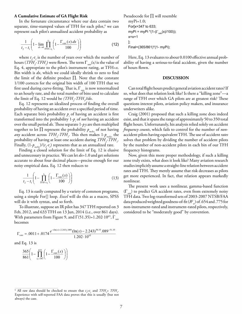
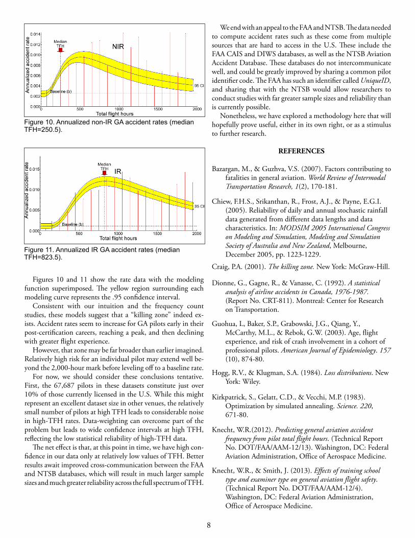
Figures 10 and 11 show the rate data with the modeling function superimposed. The yellow region surrounding each modeling curve represents the .95 confidence interval.

Consistent with our intuition and the frequency count studies, these models suggest that a “killing zone” indeed ex-ists. Accident rates seem to increase for GA pilots early in their post-certification careers, reaching a peak, and then declining with greater flight experience.

However, that zone may be far broader than earlier imagined. Relatively high risk for an individual pilot may extend well be-yond the 2,000-hour mark before leveling off to a baseline rate.

For now, we should consider these conclusions tentative. First, the 67,687 pilots in these datasets constitute just over 10% of those currently licensed in the U.S. While this might represent an excellent dataset size in other venues, the relatively small number of pilots at high TFH leads to considerable noise in high-TFH rates. Data-weighting can overcome part of the problem but leads to wide confidence intervals at high TFH, reflecting the low statistical reliability of high-TFH data.

The net effect is that, at this point in time, we have high con-fidence in our data only at relatively low values of TFH. Better results await improved cross-communication between the FAA and NTSB databases, which will result in much larger sample sizes and much greater reliability across the full spectrum of TFH.

Figure 11. Annualized IR GA accident rates (median TFH=823.5).

We end with an appeal to the FAA and NTSB. The data needed to compute accident rates such as these come from multiple sources that are hard to access in the U.S. These include the FAA CAIS and DIWS databases, as well as the NTSB Aviation Accident Database. These databases do not intercommunicate well, and could be greatly improved by sharing a common pilot identifier code. The FAA has such an identifier called UniqueID, and sharing that with the NTSB would allow researchers to conduct studies with far greater sample sizes and reliability than is currently possible.

Nonetheless, we have explored a methodology here that will hopefully prove useful, either in its own right, or as a stimulus to further research.

REFERENCES

Bazargan, M., & Guzhva, V.S. (2007). Factors contributing to fatalities in general aviation. World Review of Intermodal Transportation Research, 1(2), 170-181.

Chiew, F.H.S., Srikanthan, R., Frost, A.J., & Payne, E.G.I. (2005). Reliability of daily and annual stochastic rainfall data generated from different data lengths and data characteristics. In: MODSIM 2005 International Congress on Modeling and Simulation, Modeling and Simulation Society of Australia and New Zealand, Melbourne, December 2005, pp. 1223-1229.

Craig, P.A. (2001). The killing zone. New York: McGraw-Hill.

Dionne, G., Gagne, R., & Vanasse, C. (1992). A statistical analysis of airline accidents in Canada, 1976-1987. (Report No. CRT-811). Montreal: Center for Research on Transportation.

Guohua, L, Baker, S.P., Grabowski, J.G., Qiang, Y., McCarthy, M.L., & Rebok, G.W. (2003). Age, flight experience, and risk of crash involvement in a cohort of professional pilots. American Journal of Epidemiology. 157 (10), 874-80.

Hogg, R.V., & Klugman, S.A. (1984). Loss distributions. New York: Wiley.

Kirkpatrick, S., Gelatt, C.D., & Vecchi, M.P. (1983). Optimization by simulated annealing. Science. 220, 671-80.

Knecht, W.R.(2012). Predicting general aviation accident frequency from pilot total flight hours. (Technical Report No. DOT/FAA/AAM-12/13). Washington, DC: Federal Aviation Administration, Office of Aerospace Medicine.

Knecht, W.R., & Smith, J. (2013). Effects of training school type and examiner type on general aviation flight safety. (Technical Report No. DOT/FAA/AAM-12/4). Washington, DC: Federal Aviation Administration, Office of Aerospace Medicine.

Figure 10. Annualized non-IR GA accident rates (median TFH=250.5).

9

Mackey, J.B. (1998). Forecasting wet microbursts associated with summertime airmass thunderstorms over the southeastern United States. Unpublished MS Thesis, Air Force Institute of Technology.

Mills, W.D. (2005). The association of aviator’s health conditions, age, gender, and flight hours with aircraft accidents and incidents. Unpublished Ph.D. dissertation. University of Oklahoma, Health Sciences Center Graduate College, Norman, OK.

National Transportation Safety Board. (2011). User-downloadable database. Downloaded May 26, 2011 from www.ntsb.gov/avdata.

Sherman, P.J. (1997). Aircrews’ evaluations of flight deck automation training and use: Measuring and ameliorating threats to safety. Unpublished doctoral dissertation. The University of Texas at Austin.

Spanier, J. & Oldham, K.B. (1987). An atlas of functions. New York: Hemisphere.

Wolfram Mathematica Documentation Center. (2008). Some notes on internal implementation. Downloaded April 29, 2011 from http://reference.wolfram.com/mathematica/note/SomeNotesOnInternalImplementation.html#20880