Presidential Particularism Distributing Funds between

Alternative Objectives and Strategies

Thomas Stratmann and Joshua Wojnilower

January 2015

MERCATUS WORKING PAPER

Thomas Stratmann and Joshua Wojnilower. “Presidential Particularism: Distributing Funds between Alternative Objectives and Strategies.” Mercatus Working Paper, Mercatus Center at George Mason University, Arlington, VA, January 2015. http://mercatus.org/publication /presidential-particularism-distributing-funds-between-alternative-objectives. Abstract While recent empirical evidence supports the notion of presidential particularism—that presidents distribute federal funds to certain groups of voters in order to achieve their own political objectives—work associated with that evidence does not distinguish between presidents’ alternative objectives, nor between their alternative strategies for attaining those objectives. Using monthly US data on project-grant awards in 2009 and 2010, we study which objectives presidents pursue in distributing resources. We also address theoretical and empirical ambiguities regarding when and which congressional districts receive distributive benefits. Our results show that core constituencies of the president’s party receive more federal funding in both presidential and congressional elections. Districts represented by moderate members of both parties and partisan members of the president’s party do not, however, benefit from funding advantages before votes on important legislation. These results indicate that the president attempts to use distributive benefits to influence presidential and congressional election votes, but not votes of federal legislators. JEL codes: D72; D73; H50 Keywords: pork-barrel politics, presidential particularism, congressional particularism, distributive politics, elections, legislation, Congress Author Affiliation and Contact Information Thomas Stratmann University Professor of Economics and Law Department of Economics, George Mason University tstratma@gmu.edu Joshua Wojnilower PhD student Department of Economics, George Mason University jwojnilo@gmu.edu All studies in the Mercatus Working Paper series have followed a rigorous process of academic evaluation, including (except where otherwise noted) at least one double-blind peer review. Working Papers present an author’s provisional findings, which, upon further consideration and revision, are likely to be republished in an academic journal. The opinions expressed in Mercatus Working Papers are the authors’ and do not represent official positions of the Mercatus Center or George Mason University.

3

Presidential Particularism

Distributing Funds between Alternative Objectives and Strategies

Thomas Stratmann and Joshua Wojnilower

I. Introduction

The term “congressional particularism” refers to legislators’ deliberate allocation of federal

funds to politically influential constituencies in order to achieve certain objectives, usually

reelection. Early work on distributive politics suggested that this congressional particularism

could be balanced by “presidential universalism.” The widely held belief among scholars of

distributive politics was that, because a president’s constituency encompasses the entire nation,

presidents would pursue a distribution of federal funds that is relatively independent of their

constituents’ political characteristics (Kiewiet and McCubbins 1988; Fitts and Inman 1992;

Kagan 2001; Lizzeri and Persico 2001). Recent scholarship, however, theoretically (Fleck 1999;

McCarty 2000) and empirically (Shor 2004; Larcinese, Rizzo, and Testa 2006; Bertelli and

Grose 2009; Berry, Burden, and Howell 2010; Berry and Gersen 2010; Kriner and Reeves 2012;

Albouy 2013; Kriner and Reeves 2014) demonstrates that presidents, like legislators, do

influence the distribution of federal funds to target politically influential constituencies. In other

words, presidents are particularistic too.

Building on this literature, we attempt to determine whether presidents target specific

constituencies to influence their own reelection chances, the reelection chances of their

copartisan representatives, or legislators’ votes on important legislation. We also test alternative

hypotheses about which specific constituencies presidents will target to achieve the

aforementioned objectives. In terms of influencing electoral votes, either presidential or

congressional, presidents must choose between targeting core voters (Cox and McCubbins 1986)

4

and swing voters (Lindbeck and Weibull 1987). In terms of influencing legislators’ votes, a

president’s optimal strategy for ensuring passage of preferred legislation may include targeting a

bill’s current supporters or its moderate opposition voters, or simply refraining from providing

any distributive benefits (Groseclose and Snyder 1996). Using a new database that tracks the

monthly distribution of project-grant awards, we analyze federal spending obligations during

2009 and 2010 to test which theory or theories best fit our data for each presidential objective.

As we explain in section IV, federal project grants are highly discretionary and therefore highly

susceptible to political influence.

Our results show that the president attempts to influence presidential and congressional

election votes, but not legislative votes, through preferential distribution of federal funds. More

specifically, administrative agencies award a disproportionately higher share of federal funds to

districts within core Democratic states and core Democratic congressional districts, those

generally represented by a member of the president’s party. That share does not, however,

expand further during months immediately preceding a congressional election, when

constituents’ votes may be relatively more susceptible to political influence. Lastly, shares of

federal funding to districts represented by partisan legislators of the president’s party and

moderate legislators of both parties did not increase in months immediately before House votes

on the Dodd-Frank Wall Street Reform and Consumer Protection Act (Dodd-Frank) or the

Patient Protection and Affordable Care Act (PPACA).

Consistently with previous literature (Berry, Burden, and Howell 2010; Berry and Gersen

2010; Kriner and Reeves 2012; Albouy 2013; Kriner and Reeves 2014), we document that

districts represented by a member of the president’s party are favored in the budgetary process.

Separately, we find that members of committees with substantial influence over budgetary

5

decisions, i.e., Appropriations and Ways and Means, are unable to command a greater share of

project-grant funding for their constituencies. These results offer further support for the idea that

Congress, at least recently, lacks influence over the distribution of certain federal funds, and that,

at least with respect to these funds, presidential particularism is more important than

congressional particularism.

Beyond these findings, we consider whether certain executive agencies are more

politically motivated than others based on their individual distributions of federal funds to

politically influential congressional districts. Our analysis includes four individual executive

agencies that account for a substantial portion of project-grant funding and that previous literature

identifies as being relatively more amenable to politically targeting federal funding (Berry,

Burden, and Howell 2010).1 We find that project-grant awards by the departments of Health and

Human Services, Education, and Agriculture disproportionately favor Democratic districts, in

particular core and partisan Democratic districts, which is consistent with relatively high political

motivation. Project grant awards by the Department of Transportation, in contrast, demonstrate

minimal party favoritism, hence indicating relatively little political motivation. This result for the

Department of Health and Human Services contradicts expectations based on a previous finding

of relatively low politicization2 within that department (Berry and Gersen 2010).

In the next section we describe various theories and corresponding evidence regarding

distributive politics. Although that literature is notably Congress-centric, our focus is on recent

1 Consistently with Berry, Burden, and Howell (2010), we define political motivation in terms of favoring one party over another in the distribution of federal funds. Relatively high political motivation therefore implies that an executive agency distributes federal funds disproportionately between political parties, and relatively low political motivation implies that an executive agency distributes federal funds proportionately. This definition, however, prevents us from distinguishing between those agencies that distribute funds proportionately because they are not subject to much political influence and those that do so because they are subject to bipartisan influences. 2 Berry and Gersen (2010) define “politicization” as the ratio of political appointees to career civil servants within upper management.

6

efforts to place the president more at the center in distributive politics. Section III describes

alternative hypotheses regarding which political jurisdictions presidents optimally target to

achieve different objectives. Section IV describes our methodology and data. Section V presents

our main results. Section VI discusses robustness checks and extensions of our results, and

section VII concludes.

II. Influence of Presidents over Spending

Distributive benefits are government spending acquired through the use of political influence

(Alvarez and Saving 1997). The study of distributive politics usually analyzes federal spending,

and it focuses on the manner and degree to which Congress and the president exercise control

over the distribution of that spending. Since Congress holds the power to authorize and

appropriate federal funds, scholarship within this field has tended to focus on Congress. Both

theoretical and empirical studies have sought to determine which legislators or groups of

representatives are more successful in directing federal outlays to their constituents (Shepsle and

Weingast 1981, 1987; Weingast and Marshall 1988; Levitt and Snyder 1995, 1997; Knight 2005;

Gimpel, Lee, and Thorpe 2012; Albouy 2013).

From a theoretical perspective, congressional committees and political parties are the

organizations that can most readily influence the allocation of federal spending. This is, in part,

because Congress holds the “power of the purse.” Despite strong theoretical support for

Congress’s effectiveness in controlling the bureaucracy, attempts to test these hypotheses show

mixed results. Support comes from studies by Levitt and Snyder (1995), Alvarez and Saving

(1997), Knight (2005), Berry and Gersen (2010), and Albouy (2013). Failure to support these

7

hypotheses comes from studies by Berry, Burden, and Howell (2010), Gimpel, Lee, and Thorpe

(2012), and Kriner and Reeves (2014).

A congressional representative’s motive for engaging in distributive politics is

presumably to win reelection. Representatives that increase “pork barrel” spending for their

individual districts will fare better in elections, assuming voters reward politicians for

distributive benefits. Theory predicts that, as a result of these incentives, aggregate distributive

benefits are inefficiently large. Although presidents also seek to win reelection, their nationwide

constituency, in theory, reduces incentives to increase funding for any individual district or state.

Distributive politics scholars therefore often assume a president’s actions will limit Congress’s

inefficient spending (Kiewiet and McCubbins 1988; Fitts and Inman 1992; Kagan 2001; Lizzeri

and Persico 2001). A president’s formal powers, i.e., those established by law, receive the

greatest attention within this literature (Kiewiet and McCubbins 1988; Dearden and Husted

1990; Grier, McDonald, and Tollison 1995; McCarty 2000). The power to veto legislation is a

prominent example of a president’s formal powers. By merely threatening to veto particularistic

legislation, presidents can influence the budgetary process toward more universalistic outcomes

(Dearden and Husted 1990; Grier, McDonald, and Tollison 1995; McCarty 2000). This

assumption of presidential universalism, whereby the desired distribution of federal funds is

distinct from the political characteristics of constituencies receiving funds, supports “strong

normative arguments for increasing executive power in the legislative process” (McCarty 2000,

p. 118). However, recognizing the mixed evidence for congressional particularism, some

scholars have begun to question previous assumptions within the field of distributive politics.

Beyond their formal powers, presidents’ potential influence over the bureaucracy

includes informal abilities such as proposal power and the ability to direct administrative

8

agencies to comply selectively with federal earmarks. “Proposal power” refers to the ability to

set the agenda of political negotiations by making prominent proposals for legislative action,

which other politicians then have to respond to. While proposal power is often cited as an

advantage held by certain representatives and coalitions in Congress (Weingast 1987; Knight

2005), it may actually be the executive that has greater effective proposal power, because

presidents publish their budget proposals before representatives determine the actual budget.

Evidence suggests that presidents’ budgets heavily influenced Congress’s proposals in the

decades following World War II (Schick 2007). In recent years, however, the influence of

presidents’ budgets has been diminishing greatly, due to the growth of entitlement spending and

the increasing involvement of special-interest groups, among other factors (Schick 2007).

A president’s other informal powers include directing administrative agencies to comply

selectively with federal earmarks. Porter and Walsh (2006) demonstrate that the use of

congressional earmarks has risen dramatically in recent decades. Because Congress officially

authorizes and appropriates funds for earmarks, the process is often associated with

congressional particularism (Porter and Walsh 2006). However, earmarks are generally

contained in legislative history and therefore are not binding for administrative agencies (Berry

and Gersen 2010). Administrative agencies thus have the ability to comply selectively with

earmarks, and they may do so in order to attain other objectives. Stein and Bickers (1997, p. 50)

claim those other objectives include “stable and increasing budgets, larger staffs and additional

resources.” If Congress primarily controls federal funding, hence agency budgets, then

administrative agencies will probably comply with legislated earmarks (Porter and Walsh 2006).

However, if presidents have significant discretion in allocating federal funds to agencies, then

the agencies may only comply with earmarks that aid the president’s objectives. Presidents may

9

also exert influence over agencies’ compliance with certain earmarks by assigning political

appointments within agencies to individuals who are loyal to the president and presumably hold

similar political biases.

Whether presidents pursue a universalistic or particularistic distribution of federal funds

is an empirical question.3 While a president’s constituency does comprise an entire nation, the

electoral college system encourages concentrating election campaign efforts on select

constituencies (Lizzeri and Persico 2001), such as states or districts within states. Kriner and

Reeves (2012) provide evidence that voters reward presidents for allocating a greater share of

federal outlays to their districts. Presidents wishing to remain in office therefore have incentives

to persuade potentially decisive voters by directing a disproportionate share of federal funds to

their districts.

Although a president might want to target decisive voters, it is not straightforward for

researchers to determine whether core or swing voters are the decisive ones from the president’s

point of view. On the one hand, scholars contend that the electoral college system incentivizes

candidates to focus their efforts on swaying voters within swing states (Bartels 1985; Nagler and

Leighley 1992). Kriner and Reeves (2014) provide evidence for this supposition, showing that

presidents target swing states. On the other hand, distributing “pork” to voters within core states,

that is, those states that strongly supported a president’s party in prior elections, could be a more

cost-effective means of improving one’s odds (Cox 2010). Supporting this hypothesis, Larcinese,

Rizzo, and Testa (2006) find evidence that incumbent presidents target core states.

3 It is important to note that pursuit of a universalistic distribution and pursuit of a particularistic distribution of federal funds are not necessarily mutually exclusive. The pursuit of both types of distribution could occur at different times throughout a president’s tenure in office.

10

This debate about whether presidents target swing or core voters carries over into

presidents’ role as party leader. This responsibility likely entails pressure to convey privileges

on members of the president’s own party. More specifically, an administration may seek to

advantage its own party members in congressional elections by selectively distributing federal

funds to districts currently represented by copartisan members. Previous empirical studies

find evidence that districts represented by members of a president’s party receive a

disproportionate share of federal funding (Berry, Burden, and Howell 2010; Berry and Gersen

2010; Kriner and Reeves 2012; Albouy 2013; Kriner and Reeves 2014). Mixed evidence

exists, however, regarding whether these funds favor swing or core districts. For example,

Berry and Gersen (2010) provide evidence that presidents favorably target swing districts. In

contrast, Kriner and Reeves (2014) provide some evidence that core districts receive a higher

share of federal spending.

Although a president can lobby for specific legislation, Congress ultimately passes

bills. A president’s lobbying success therefore depends on the president’s ability to influence

legislators’ votes. This presents another potential strategy for targeting federal funds. Levitt

and Snyder (1997) find that representatives are more likely to be reelected if their constituents

receive extra federal funding. Presidents, then, may be able to further their agendas by

allocating federal outlays to the districts of representatives whose votes are critical to their

goals. However, determining which legislators represent the critical votes is, once again, a

difficult task. Furthermore, the empirical evidence for which specific congressional votes

presidents are using federal funds to sway is relatively sparse, at least in part because the

yearly data make it difficult to distinguish between outlays intended to garner support for

different pieces of legislation.

11

III. Hypotheses

Recent scholarship in distributive politics suggests that presidents seek a distribution of federal

spending based on the political characteristics of their constituents, contrary to the previously

prevailing assumption of presidential universalism (see, for example, Berry, Burden, and Howell

2010 and Kriner and Reeves 2014). Theoretically, we posit that presidents hold three alternative

objectives which they may aim to achieve at any given point in time:4 First, presidents aim to

win reelection. Second, presidents aim to support their party members in congressional elections.

This creates a party composition of legislators in Congress that is generally more likely to

support the president’s agenda. Third, presidents promote a specific legislative agenda.

Presidents must also choose among alternative strategies for effectively targeting limited federal

funds for each of these objectives.

Presidents seeking to secure their own reelection (or the election of their party’s next

presidential candidate) face a tradeoff between targeting swing and core voters. Theoretical

models can offer support for either strategy, depending on what assumptions are used. Lindbeck

and Weibull (1987) consider a two-party system where ideological preferences are exogenous,

targeted redistributions determine voter preferences, and candidates, such as the president, are

equally certain about the responses of core and swing voters to distributive benefits. Swing

voters, who are ideologically moderate, require relatively less distributive benefits than strongly

partisan voters to sway their votes. According to Lindbeck and Weibull, therefore, politicians

will compete for swing votes. Cox and McCubbins (1986) analyze a similar model but allow for

uncertainty regarding the responses of core and swing voters to distributive benefits. Assuming

4 A fourth objective, posited by Cann and Sidman (2011) in reference to congressional particularism, is a desire to reward party loyalty. This method of distributing benefits is, however, consistent with achieving each of the other objectives, and therefore we do not consider it independently.

12

that a president holds an information advantage about core constituents, the preferable strategy

becomes dependent on the president’s risk-tolerance level. Risk-averse presidents, who receive

greater utility from less relative uncertainty, will target core constituents. Risk-neutral or risk-

loving presidents, on the other hand, will target marginal, i.e., swing, constituencies.

Dixit and Londregan (1996) compare this basic model with one that incorporates a

different information advantage. Instead of uncertainty regarding how types of voters will

respond to distributive benefits, candidates hold an information advantage in the types of benefits

that provide the most utility to core constituents. As well as generating similar predictions as the

model by Lindbeck and Weibull (1987), Dixit and Londregan’s (1996) model predicts that with

symmetrical information, groups with relatively large proportions of moderate (swing) voters

will receive more distributive benefits. Senior citizens, for example, are therefore likely to

receive a disproportionately favorable allocation of federal funds, while urban minorities receive

less funding. Separately, Dixit and Londregan’s model predicts that voters with lower incomes

will receive a federal funding advantage, because the marginal utility of allocating a dollar in

redistributive benefits to this group is higher. Alternatively, using the assumption of

asymmetrical information, Dixit and Londregan (1996) attain similar results to Cox and

McCubbins (1986).

Presidents also confront a tradeoff between swing and core voters in deciding the most

cost-effective means of increasing their party’s representation within Congress. The

aforementioned theories focus on basic models with two candidates vying for a single district.5

Ward and John (1999, p. 35) consider a similar model to those just described, in which two

political parties are competing “to maximize the number of seats they expect to win in national-

5 In terms of presidential elections, the single district is the entire nation.

13

level elections.” Retaining the assumption of symmetrical information regarding voter responses,

Ward and John predict that political parties will not simply target any swing voter, but rather

marginal opposition constituencies—voters who normally support the president’s opposition but

might be willing to vote for the president’s side. The only constituency along the core versus

swing voter spectrum that theory does not support targeting is therefore core opposition voters.

Promoting a specific legislative agenda through distributive benefits, as opposed to using

distributive benefits to increase election chances, may entail a different set of incentives for

distributing federal funds. The early literature on coalition formation and vote buying using a

single-vote-buyer model generally assumes or predicts that minimal winning coalitions will arise

in equilibrium (Denzau and Munger 1986; Baron and Ferejohn 1989). Winning coalitions within

Congress, however, frequently exceed the minimal size necessary.

Attempting to explain this difference between theory and empirical data, Groseclose and

Snyder (1996) analyze a model with two competing vote buyers that move sequentially.

Depending on the initial distribution of voter preferences, there are three unique equilibriums in

which a given vote buyer, such as the president, wins. These scholars predict that (1) if there is

minimal opposition within the initial distribution of legislator preferences, then a president’s

preferred legislation can win a majority of votes without providing distributive benefits to any

legislators. (2) If the initial distribution is more even, but favors a president’s position, then a

president’s preferred legislation can win a majority of votes by sufficiently raising the opposition

party’s cost of buying votes. Somewhat counterintuitively, this strategy entails a president

effectively paying off legislators that already support the president’s position. (3) If the initial

distribution is relatively even, but favors the opposition party’s position, a president’s preferred

legislation can win a majority of votes by adopting a “leveling strategy.” This strategy involves

14

buying votes such that the opposition’s costs of paying off any legislator in the new

supermajority are equal. In this equilibrium, a president will therefore provide relatively more

distributive benefits to moderate voters, especially those of the opposition party.

These theories highlight different possible optimal strategies for selecting which types of

voters to target. And the results of the scholarly work on the theory of distributive benefits are

ambiguous. Our novel data set will help to discriminate empirically among the alternative

hypotheses described above.

A separate consideration is the mechanism by which a president can influence the

distribution of federal spending. The structure and process theory, articulated by McCubbins,

Noll, and Weingast (1989, p. 481), contends “that the main avenue for controlling bureaucrats is

to place ex ante procedural constraints on the decisionmaking process.” Stemming from this

theory, two factors that likely influence an agency’s spending decisions are their specific mission

and the relative influence of political appointees and career civil servants over funding decisions

(Berry and Gersen 2010). Berry and Gersen (2010) quantify these considerations by constructing

measures of Democratic tilt6 and politicization within an agency.

Berry, Burden, and Howell (2010) identify four specific agencies that account for a

substantial amount of high-variation spending and are frequently associated with “pork” in

scholarly literature.7 These are the Department of Health and Human Services (which accounts

for 24.2% of project-grant funding during our study), the Department of Education (15.22%), the

Department of Transportation (14.81%), and the Department of Agriculture (7.17%). Based on

6 “Democratic ‘tilt’ . . . is defined as the ratio of an agency’s annual outlays going to Democratic controlled districts relative to the share of seats in the House controlled by Democrats” (Berry and Gersen 2010, p. 9). 7 Previous studies within distributive-politics literature often employed a database that included federal spending through all federal programs. Levitt and Snyder (1995) devised a method to separate federal spending into high- and low-variation programs to determine which category was easier to manipulate. High-variation spending therefore refers to spending through federal programs that are especially variable and hence subject to greater discretion.

15

Berry and Gersen’s (2010) measures of Democratic tilt and politicization, we hypothesize that

the Departments of Education and Agriculture will display the strongest political bias while the

Departments of Health and Human Services and Transportation will display relatively weak

political bias.

IV. Methodology and Data

For our analysis, federal spending data come from USAspending.gov, a government compendium

of federal programs. Within this database, our analysis focuses on data provided through the

FAADS Plus system. FAADS Plus documents grants, loans, direct payments, and other assistance

transactions from fiscal year (FY) 2007 onward. Thirty-one departments and agencies of the

executive branch of the federal government submit assistance-award actions directly to

USAspending.gov through this system. Unlike the basic FAADS system, FAADS Plus permits

restricting our analysis to federal project grants, a category of spending particularly amenable to

political influence (Levitt and Snyder 1995; Bertelli and Grose 2009). The following brief

description of the awards process highlights the discretionary nature of federal project grants.

Congress provides the initial details for a federal project grant through authorizing

legislation. Although authorizing legislation “may establish application eligibility and, to varying

degrees, eligible activities, federal agencies exercise broad discretion in administering the grant

program. Administering federal grant programs may include establishing procedures for

applying, reviewing, scoring, and awarding federal grants” (Keegan 2012). Since agencies award

federal project grants on the basis of merit, they must exercise some discretion during each step

of the award process.

16

The complete database tracks the total dollar amount awarded to recipients in each of 435

congressional districts. In this database, awards refer to dollars obligated, not outlays or

expenditures, which have been used in previous studies. To determine whether awards are more

appropriately categorized by the month in which projects are obligated or actually start, we

consider the credit-claiming process of politicians. A common practice among politicians is

publicly claiming credit for project grants at the time an agency announces the award. For

example, in September 2010 Representative Richard E. Neal (D-MA) announced, from police

headquarters, that the US Justice Department had awarded the Springfield Police Department a

federal grant of $267,703 (Goonan 2010). Separately, in October 2010 Representative Henry

Cuellar (D-TX) announced that the Department of Education awarded Texas A&M International

University two federal grants summing to $6,061,035 (Texas A&M International University

2010). Given this credit-claiming process, we categorize federal grant awards by the month in

which funds are initially obligated.

Although documentation of transactions in USAspending.gov began in FY 2007, we

restrict our study to calendar year (CY) 2009 and CY 2010, which encompass the 111th US

Congress. As of April 2014, complete spending data were only available for this one

congressional session. Within the 111th US Congress, 11 districts replaced representatives for

various reasons. To avoid issues regarding replacements during the period under consideration,

we remove these 11 districts from our database. With 24 months of data for the remaining 424

districts, our total sample includes 10,176 district-by-month observations. This sample consists

of project-grant awards data for 28 individual departments and agencies. We excluded the

Executive Office of the President, the Social Security Administration, and the Department of

Veterans Affairs because they either did not obligate funds or failed to report obligations during

17

this period. Further, our sample includes 1,381 district-months where zero grant dollars were

obligated. To account for months with zero grant dollars obligated, we add $1 to each district-

month before transforming expenditure data into natural logarithms. In total, our database tracks

approximately $45.1 billion in federal expenditures. The inflation-adjusted total spending in real

2009 dollars is about $44.2 billion, which, per year, is equivalent to essentially $52 million per

district and $75 per capita. Monthly per capita obligations to districts range from $0 to $382.

Despite focusing on presidential particularism, we do not argue that presidents and, by

extension, federal agencies solely determine the flow of federal funds to a district. A number of

other factors and actors, such as senators and governors, some of which might be unobservable

to the analysts, may also influence project-grant awards. To control for some of these factors we

include several indicator variables.

We specify the following basic regression model:

ln(𝑜𝑏𝑙𝑖𝑔𝑎𝑡𝑖𝑜𝑛𝑠!") =  𝛽! +  𝛽!𝑷𝒊𝒕 +  𝛽!𝑷𝒊𝒕𝑽𝒊𝒕 +  𝛽!𝑿𝒊𝒕 +  𝜀!" (1)

where subscript i denotes congressional districts and t denotes the month. The dependent variable

is the log of real per capita federal funds obligated through project grants to a congressional

district. We will estimate three alternative specifications of equation 1.

Our first specification tests the hypothesis that presidents distribute federal funds to select

constituencies in order to influence voter behavior in presidential elections, thereby increasing

their party’s chance of remaining in the White House. This specification tests whether districts

within core or swing states receive greater distributive benefits and whether those benefits

increase before congressional elections. The 𝑷𝒊𝒕 vector includes three indicator variables

distinguishing between districts in core and swing states. Like Kriner and Reeves (2014), we

define core and swing states based on a party’s average state-level vote percentage in the

18

preceding three presidential elections. Core Democratic states are those where the Democratic

presidential candidate received, on average, more than 55 percent of the electoral vote.8 Swing

states are those where neither party’s presidential candidate received, on average, more than 55

percent of the vote. Core Republican states, those where the Republican presidential candidate

received, on average, more than 55 percent of the electoral vote, are the excluded category.

In this first specification, the first indicator variable in the 𝑷𝒊𝒕 vector equals one if a

district is within a core Democratic state. The second indicator variable in the 𝑷𝒊𝒕 vector equals

one if a district is within a swing state where the president received a larger share of the two-

party vote in the most recent presidential election, i.e., 2008.9 The final indicator variable in the

𝑷𝒊𝒕 vector equals one if a district is within a swing state where the president did not receive the

largest share of the two-party vote in the most recent presidential election.10 This variable

measures whether presidents attempt to increase their reelection chances by winning over new

swing states in the next election.

The 𝑽𝒊𝒕 vector includes three month indicators to test for changes in total funding before

important electoral and legislative votes. The first month indicator equals one if a project-grant

obligation began in either September or October 2010. This variable measures whether

obligations increased in months immediately preceding the congressional election on November

2, 2010. The second month indicator equals one if an obligation began in either October or

8 The specific cutoff level selected could bias our data if the maximum funding level is associated with a Democratic vote share in the middle of our distribution. To test whether this issue exists, we estimated the following quadratic equation: 𝑦 = 𝛽! +  𝛽!𝑺𝒊𝒕 +  𝛽!𝑆!"! +  𝛽!𝑿𝒊𝒕 +  𝛿! +  𝜀!", where S is the average Democratic vote share in the previous three presidential elections. Using this estimate, we find that the maximum funding level is associated with an average Democratic vote share of nearly 97%. Since this percentage exceeds all values within our database, funding levels do not decrease even for the strongest core districts. 9 This implies that the president’s party received, on average, less than 55 percent of the electoral vote in the three previous presidential elections, but the president won the two-party vote share in the most recent election. 10 This implies that the president’s opposition party received, on average, less than 55 percent of the electoral vote in the three previous presidential elections, but the opposing candidate won the two-party vote share in the most recent election.

19

November 2009. This variable measures whether obligations increased in the months preceding a

House vote on the Dodd-Frank Wall Street Reform and Consumer Protection Act (Dodd-Frank),

which occurred on December 11, 2009. The third month indicator equals one if an obligation

began in either February or March 2010 and zero otherwise. This variable measures whether

obligations increased in the months preceding the House vote on the PPACA that took place on

March 21, 2010. We allow for a differential effect in relative funding shares before important

electoral and legislative votes by including interaction terms between these indicator variables

and the 𝑷𝒊𝒕 vector.

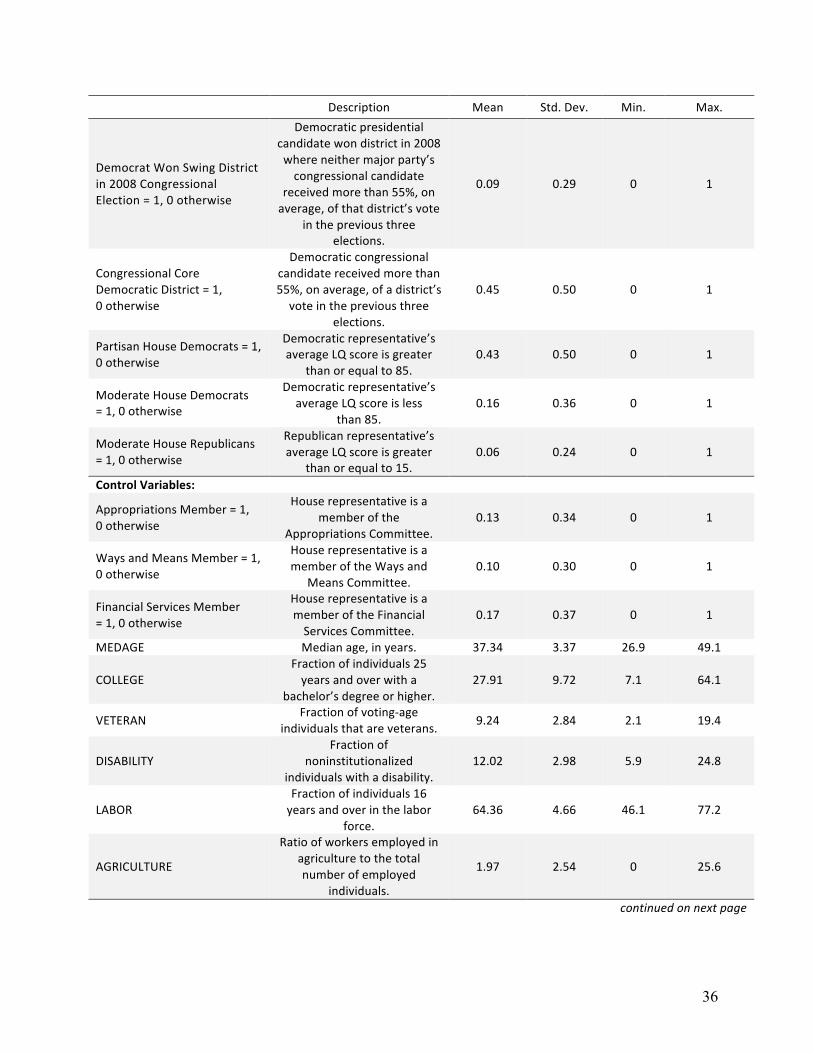
The 𝑿𝒊𝒕 vector includes several control variables to account for individual legislator

characteristics that may be favorable to attaining a disproportionate share of federal funds. We

include two indicator variables, capturing whether a House representative is a member of the

Appropriations or the Ways and Means committees. Previous literature on distributive politics

identifies membership on these two committees, in particular, as being favorable to obtaining

federal funds. Beyond its general position of power within the House, the latter committee was

also responsible for bringing the PPACA to the House floor for a vote. We allow for a

differential effect in relative funding shares before the House vote on the PPACA by including

an interaction term between the Ways and Means indicator variable and the PPACA month

indicator. Similarly, the Financial Services committee was responsible for bringing Dodd-Frank

to the House floor for a vote. We therefore include an indicator variable capturing whether a

representative is a member of the Financial Services committee. To test for a differential effect in

relative funding shares before the House vote on Dodd-Frank we also include an interaction term

between that indicator variable and the Dodd-Frank month indicator.

20

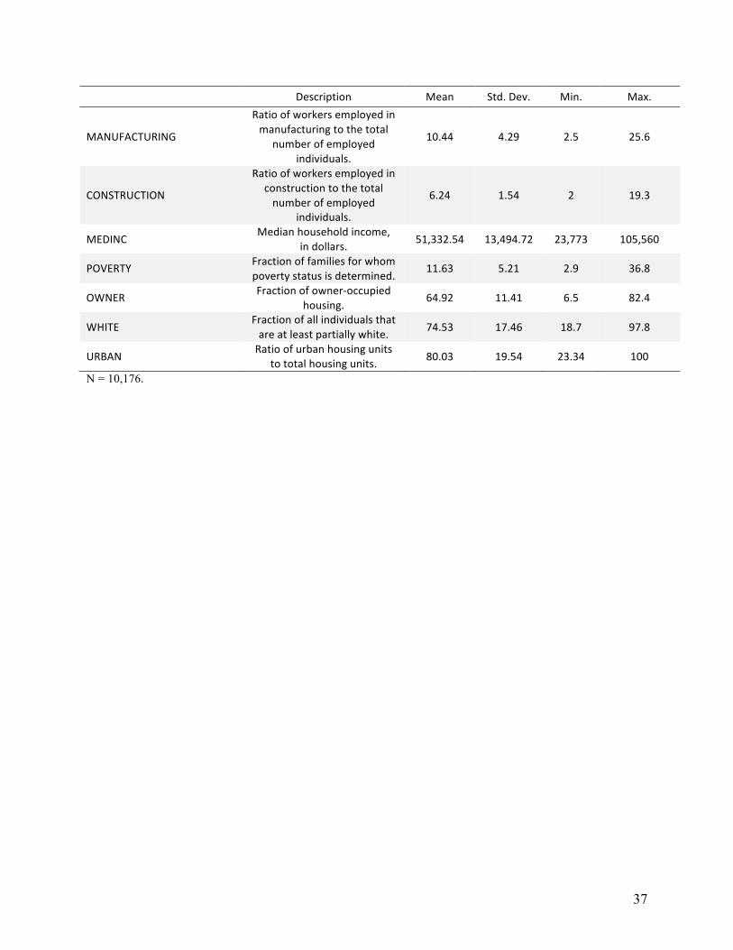
The 𝑿𝒊𝒕 vector also includes several control variables to account for district-level

demographics, which may affect the distribution of federal funds. MEDAGE is the median age

expressed in year, COLLEGE is the fraction of individuals 25 years and over with a bachelor’s

degree or higher, VETERAN is the fraction of voting-age individuals who are veterans,

DISABILITY is the fraction of noninstitutionalized individuals with a disability, LABOR is the

fraction of individuals 16 years and over in the labor force, AGRICULTURE is the ratio of

workers employed in agriculture to the total number of employed individuals,

MANUFACTURING is the ratio of workers employed in manufacturing to the total number of

employed individuals, CONSTRUCTION is the ratio of workers employed in construction to the

total number of employed individuals, MEDINC is the log-level of median household income

expressed in dollars, POVERTY is the fraction of families who live below the poverty line,

OWNER is the fraction of owner-occupied housing, WHITE is the fraction of all individuals that

are at least partially white, and URBAN is the ratio of urban housing units to total housing

units.11 The 𝑽𝒊𝒕 and 𝑿𝒊𝒕 vectors are exactly the same in all three specifications. The error term is

consistently 𝜀!" and we cluster all standard errors by congressional district.

Before describing the other two model specifications, it is informative to consider some

similarities and differences between our general model specification and others employed within

the distributive-politics literature, particularly in those works focused on the president’s role.

More specifically, we consider the decisions by other authors to account for observable and

unobservable time-invariant district-level characteristics by including either fixed effects (Berry,

Burden, and Howell 2010; Berry and Gersen 2010; Kriner and Reeves 2012; Kriner and Reeves

2014), district-level demographics (Bertelli and Grose 2009), or both (Shor 2004; Larcinese, 11 These data were obtained from the US Census Bureau Download Center (http://factfinder2.census.gov/faces/nav /jsf/pages/download_center.xhtml).

21

Rizzo, and Testa 2006; Albouy 2013). Identification within those models that incorporate fixed

effects is constrained to within-district changes over time. However, our hypotheses relate to

differences in federal funds obligations between districts, both at points in time and over time. As

a result, our model specification explicitly controls for district-level demographics but does not

include district-level fixed effects.

Our second specification tests the hypothesis that presidents disproportionately distribute

federal funds to influence voter behavior in congressional elections and thus increase the

president’s number of congressional copartisans in the House. This specification also tests whether

core or swing districts receive greater distributive benefits and whether those benefits increase

before congressional elections. As with the previous specification, the 𝑷𝒊𝒕 vector includes three

indicator variables distinguishing between core and swing districts. We define core and swing

districts by using the average vote percentages from the three previous congressional elections, not

presidential elections. Core Democratic districts are therefore those where a Democratic

congressional candidate received, on average, more than 55 percent of the vote. We define swing

districts as those where neither party’s congressional candidate received, on average, more than 55

percent of the popular vote. Core Republican districts, those where a Republican congressional

candidate received, on average, more than 55 percent of the vote, are the excluded category.

In this second specification, the first indicator variable in the 𝑷𝒊𝒕 vector equals one for

core Democratic districts. The second indicator variable in the 𝑷𝒊𝒕 vector equals one for swing

districts where the Democratic candidate received a larger share of the two-party vote in the most

recent congressional election, i.e., 2008. The final indicator variable in the 𝑷𝒊𝒕 vector equals one

for swing districts where the Democratic candidate did not receive a larger share of the two-party

vote in the most recent congressional election. This variable measures whether presidents

22

attempt to increase their number of congressional copartisans by winning new swing districts in

the next election.

Our third specification tests the hypothesis that presidents selectively distribute federal

funds to influence a representative’s legislative votes. We further test whether the funding

disparity between districts increases before important House votes. In this specification we do

not include variables measuring swing or core districts, since our interest is in voting patterns of

current representatives. Instead, the 𝑷𝒊𝒕 vector includes indicator variables differentiating

partisan and moderate representatives of either party. We define a representative as partisan or

moderate based on his or her average Liberal Quotient (LQ) score over the two years while the

111th US Congress was in session. We obtained LQ scores from Americans for Democratic

Action (ADA). These LQ scores range from 0 to 100, with higher scores representing a more

liberal voting record. Partisan Democrats, in our definition, are those representatives with an

average LQ greater than or equal to 85. Moderate Democrats have an average LQ lower than 85.

The first indicator variable in the  𝑷𝒊𝒕 vector equals one if a district’s representative is a partisan

member of the Democratic Party. This vector also includes an indicator variable equal to one if a

district’s representative is a moderate member of the Democratic Party. The final indicator

variable included in this vector is set equal to one if a district’s representative is a moderate

member of the Republican Party. Moderate Republicans have an average LQ greater than or

equal to 15. Although these LQ scores are seemingly low barriers for consideration as a

moderate, based on these measures there are only 66 moderate Democrats and 27 moderate

Republicans out of 249 and 175 total members in each party, respectively. The distribution of

LQ scores highlights how infrequently party members broke rank during this congressional

session. The excluded category is partisan Republicans, who have an average LQ of less than 15.

23

We employ each of these three specifications to determine the president’s influence over

the distribution of all project-grant awards, as well as those of the four select agencies in

particular: the Department of Health and Human Services, the Department of Education, the

Department of Transportation, and the Department of Agriculture.

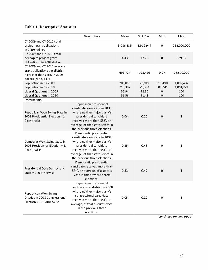
Table 1 (page 35) reports means and standard deviations of data for the 424 congressional

districts within our database during CY 2009 and CY 2010. This table also shows descriptive

statistics for the instruments and control variables used in this analysis.

V. Results

Recent scholarship places the president front and center in distributive politics. Previous

evidence confirmed that presidents act in a particularistic rather than universalistic manner but,

in general, did not differentiate among presidents’ alternative objectives (winning presidential

elections, congressional elections, and important legislative votes), nor among their alternative

distributive strategies for achieving those goals (targeting swing voters, core voters, etc.)

Focusing on the three alternative presidential objectives, we test which theory or theories best fit

our data. We discuss the results for each different objective separately.

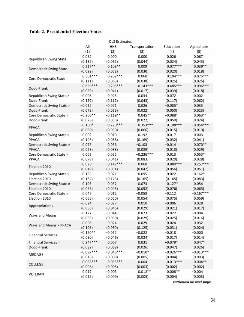
First and foremost, presidents seek to ensure their party retains control of the White

House. Table 2 (page 38) presents results of our model for this objective.

Column 1 of table 2, which includes project-grant awards data for all agencies, shows

that districts within both swing and core Democratic states receive a greater share of federal

funds than those in all Republican states. Furthermore, the funding advantage of those within

core Democratic states is more than double the advantage of districts within Democratic swing

states. To put these funding advantages in perspective, note that districts receive, on average, $52

24

million per year through project grants. An advantage of approximately 50 percent, for districts

within core Democratic states, is therefore equivalent to $26 million more per district, or $37.5

more per capita, per year. These initial results support the general hypothesis that presidents act

in a particularistic, rather than universalistic, manner. Furthermore, these results are more

consistent with the Cox and McCubbins (1986) “core voter” model, with a risk-adverse vote

buyer, than with the Lindbeck and Weibull (1987) “swing voter” model.

Turning our attention to the control variables based on individual legislator

characteristics, we find that members of the Appropriations, Ways and Means, and Financial

Services committees do not garner any overall increase in federal funds for their districts.

Although the latter groups actually experience a funding disadvantage on average, these districts

experienced a statistically significant increase in federal funds during the months immediately

preceding a House vote on Dodd-Frank. Because the Financial Services committee was

responsible for bringing the Dodd-Frank legislation to the House floor, this increase in federal

funds could conceivably have been an attempt to sway specific legislation within that bill.

Overall, our first specification therefore also supports the idea that congressional particularism is

less important in the distribution of funds than is presidential particularism.

Let us shift our discussion to individual agencies, columns 2 through 5. A couple of the

results deserve comment. First, the Departments of Health and Human Services, Education, and

Agriculture all demonstrate Democratic favoritism during this period, consistent with the fact

that Democrats held control of the White House and both Houses of Congress. Second, the

Department of Transportation demonstrates a lack of political favoritism by proportionately

distributing funds across all districts. Before going into a further analysis of these results, we first

consider the results from the other specifications.

25

Aside from influencing voters in presidential elections, presidents, as leaders of their

party, also attempt to increase their number of copartisan representatives by influencing voter

behavior in congressional elections. Table 3 (page 40) presents the results of our model for

this objective.

Column 1 of table 3, which again accounts for project-grant funding by all agencies,

demonstrates that core Democratic districts receive a disproportionately high share of federal

funds. In contrast, congressional swing districts, regardless of the representative’s party, do not

receive any statistically significant federal-funding advantage when compared to core

Republican districts. These initial results once again support the Cox and McCubbins (1986)

“core voter” model, with a risk-adverse vote buyer, over the Lindbeck and Weibull (1987)

“swing voter” model. Also noteworthy is the lack of any differential effect in relative federal-

funding shares, for swing and core districts of both parties, immediately before the 2010

congressional election. One plausible explanation for this finding is that attaining relative

increases in project-grant funding immediately before an election is an inefficient method of

temporarily boosting a representative’s vote share. Alternatively, the lack of a differential effect

may arise from agencies’ attempts to remain relatively apolitical. Further research is necessary to

determine whether it is one of these hypotheses or some other hypothesis that is most consistent

with the data.

Results in column 1 for the control variables that account for individual legislator

characteristics are again worth noting. Consistent with the findings from the previous

specification, members of the three influential committees are, on average, unable to attain a

disproportionately large share of federal funds for their districts. Districts represented by

members of the Financial Services committee do, however, once again receive a statistically

26

significant increase in federal funds during the months immediately before a House vote on

Dodd-Frank. Regarding tests for individual agencies, columns 2 through 5, the Departments of

Health and Human Services, Education, and Agriculture once again demonstrate a Democratic

bias. In this specification, however, only core Democratic districts receive a funding advantage.

In contrast, project-grant funding from the Department of Transportation still does not display

any political bias.

Apart from seeking reelection or acting as party leader, presidents pursue a legislative

agenda by influencing legislators’ votes. Table 4 (page 42) displays the results of our model for

this objective.

Focus first on the results that incorporate project-grant awards by all agencies: column 1

of table 4 shows that, in general, districts with relatively liberal representatives receive a

disproportionately high share of federal funds. The advantage for partisan Democrats is more

than double that attained by moderate Democrats, while moderate Republicans receive an even

smaller funding advantage relative to partisan Republicans. These results are consistent with our

earlier findings that districts represented by a member of the president’s party, in particular core

or partisan Democratic districts, receive favoritism in the budgetary process. However, a

differential effect in relative funding shares for the months leading up to the 2010 congressional

election remains absent from our data.

Our primary interest in this specification is, however, whether or not differential effects in

the allocation of distributive benefits occur before House votes on specific pieces of legislation.

Column 1 shows a statistically significant negative differential effect in relative funding shares for

both partisan and moderate Democratic districts during months preceding a House vote on Dodd-

Frank. This finding implies that partisan voters of the opposition party, i.e., Republicans, received

27

a relative increase in federal funds during this period, which is inconsistent with all three

equilibriums in Groseclose and Snyder (1996). This finding also appears to be inconsistent with

actual voting results, in which Democrats won the House vote with a supermajority despite not

getting a single Republican representative to vote in favor of the bill.12

In contrast to the above results, column 1 shows no differential effects in relative funding

shares for months preceding a House vote on the PPACA. This finding is consistent with an

equilibrium in Groseclose and Snyder (1996), more specifically one where a defensible

supermajority exists in the initial distribution of legislator preferences. Presidents can therefore

ensure their preferred legislation wins a majority of votes without providing any extra distributive

benefits. Actual voting results support this inference since Democrats won the House vote with a

supermajority, even though not a single Republican representative voted to pass the bill.13

Column 1 also confirms results for the individual legislator control variables seen in the

previous two specifications. Representatives on potentially influential committees do not, on

average, attain a funding advantage for their districts. Members of the Financial Services

committee were, however, seemingly able to attain an increase in federal funds for their districts

during the months before a House vote on Dodd-Frank. Overall the consistency of these findings

supports the view that Congress, at least recently, lacks influence over the distribution of certain

federal funds.

Finally, columns 2 through 5 demonstrate that all four individual agencies distribute a

greater share of project-grant funding to partisan districts of the Democratic Party. Jointly

considering results from all three specifications suggests that the Departments of Health and

12 Results for this House vote on Dodd-Frank are available at https://www.govtrack.us/congress/votes/111-2009 /h968. 13 Results for this House vote on the PPACA are available at https://www.govtrack.us/congress/votes/111-2010 /h165.

28

Human Services, Education, and Agriculture are relatively more politically motivated in their

distribution of project-grant funding. In contrast, funding by the Department of Transportation

displays minimal political bias.14 While these findings largely confirm our hypotheses regarding

relative political motivation, based on Berry and Gersen (2010), our results contradict their

finding of relatively low politicization within the Department of Health and Human Services.

VI. Robustness and Extensions

Approximately 14 percent of district-month observations in our database are zeroes; that is, there

are months when no project-grant funding obligations begin for a given district. These conditions

raise concerns about the consistency of ordinary least squares (OLS) estimates, so we also test

each specification of our model using Tobit estimation. The results of these tests, displayed in

tables 5 through 7 (pages 44–48), are largely unchanged.

It bears repeating that the limited availability of obligations data from the

USAspending.gov database severely limits this study’s time period. This paper can therefore

serve as a baseline for future research, which could use an expanded database and test similar

hypotheses. With respect specifically to data selection, there are several possible extensions of

this analysis worth pursuing. One extension involves testing whether similar results exist using

measures of federal spending distinctly different from project grants. Although project-grant

funding appears particularly amenable to political manipulation, a previous study found that

formulaic spending is more discretionary (Alvarez and Saving 1997). Moreover, presidents and

Congress may be able to exert greater influence over the distribution of federal funds depending

14 To clarify, once again, minimal political bias, in this instance, refers to a relatively proportional distribution of funds between political parties. We do not, however, test whether the proportional distribution is due to a lack of political capture or to bipartisan capture, both of which are plausible explanations for our finding.

29

on whether spending occurs through project grants or legislated formulas, respectively (Levitt

and Snyder 1995).

Separately, this study analyzes a period in which the Democratic Party held the White

House as well as a majority in both houses of Congress. We are therefore unable to distinguish

whether districts receive a disproportionate share of federal funds because their representative is

a member of the majority party or the president’s party. More recent data that includes different

parties controlling the White House and House of Representatives, when available, will aid in

distinguishing between these two potential sources of distributive benefits.

Our results also prompt new questions for future research. Contrary to some previous

evidence (Berry and Gersen 2010), swing districts with Democratic representatives did not

receive a disproportionate share of federal funds, in general or before the 2010 congressional

election. In that election, the Republican Party gained 63 seats within the House. The Blue Dog

coalition, a group of moderate Democrats, lost over half of its membership (Allen 2010). Was

this result a consequence of the decision to target core Democratic districts rather than swing

districts? While we can never know that answer with certainty, future research could test for a

relationship between this relative distribution of federal funds and election outcomes.

Another question arises from our results on influencing legislative votes. Our evidence

suggests that a defensible supermajority favoring the passage of the PPACA existed within the

initial distribution of legislator preferences, but it is inconclusive regarding the initial distribution

of legislator preferences for Dodd-Frank. Applying similar tests to other legislative votes,

particularly those that receive some bipartisan support, may provide further evidence for or

against Groseclose and Snyder’s (1996) vote-buying theories.

30

Finally, results suggest that the relative political motivation within the Department of

Health and Human Services is actually opposite what is indicated by previous evidence (Berry

and Gersen 2010). One possibility is that the ratio of political appointees to career civil servants

within upper management recently changed, adjusting the relative politicization of each agency.

Another explanation is that different types of spending, even within executive agencies, are more

or less politically motivated. Distinguishing between these and other possible interpretations

offers another compelling direction for future research.

VII. Conclusion

Distributive politics scholars spent many years almost exclusively concerned with examining

Congress’s particularistic influence over the distribution of federal funds. Some scholars took

presidential universalism for granted on the basis of the president having a nationwide

constituency (Kiewiet and McCubbins 1988; Fitts and Inman 1992; Kagan 2001; Lizzeri and

Persico 2001). Out of this assumption grew normative arguments for granting the president

greater control over the bureaucracy (Kagan 2001). During the last decade, however, empirical

evidence for presidential particularism has flourished.

Our analysis provides an attempt to differentiate between presidents’ objectives and their

particularistic strategies for attaining those objectives. We find that the president targets

politically influential constituencies to influence both presidential and congressional elections,

but not votes on important legislation. More specifically, districts within core Democratic states

and core Democratic congressional districts receive a disproportionately large share of federal

funds. This result demonstrates that the “core voter” model (Cox and McCubbins 1986), with a

risk-adverse vote buyer, is a better representation of our data than the “swing voter” model

31

(Lindbeck and Weibull 1987). Our results also demonstrate that districts represented by partisan

members of the president’s party and moderate members of both parties did not receive an

increase in their relative shares of federal funds in the months immediately preceding House

votes on Dodd-Frank or the PPACA.

Separately, our analysis considers the relative political motivations of four individual

executive agencies that account for a substantial portion of project-grant funding. We find that

the departments of Health and Human Services, Education, and Agriculture distribute project-

grant funding favorably to Democratic districts, particularly core and partisan Democratic

districts. In contrast, the distribution of project-grant funding by the Department of

Transportation displays relatively minimal political bias. This finding regarding the relative

political motivation of the Department of Health and Human Services is not consistent with that

attained by Berry and Gersen (2010).

In sum, our results add support for the presidential particularism hypothesis, under

which presidents influence the distribution of federal spending to target politically influential

constituencies. Among the alternative objectives a president aims to achieve, we show that the

president attempts to influence presidential and congressional election votes but not legislative

votes. Determining which objectives presidents seek to achieve through distributive benefits

and which specific districts benefit from presidential particularism remain appealing topics for

future research.

32

References

Albouy, D. (2013). Partisan Representation in Congress and the Geographic Distribution of Federal Funds. Review of Economics and Statistics, 95(1), 127–41.

Allen, J. (2010). Blue Dog Wipeout: Half of Caucus Gone. Politico. Nov. 3. Retrieved from http://www.politico.com/blogs/glennthrush/1110/Blue_Dog_wipeout_Half_of_caucus _gone.html.

Alvarez, R. M., & Saving, J. L. (1997). Congressional Committees and the Political Economy of Federal Outlays. Public Choice, 92(1–2), 55–73.

Baron, D. P., & Ferejohn, J. A. (1989). Bargaining in Legislatures. American Political Science Review, 83(4), 1181–206.

Bartels, L. M. (1985). Resource Allocation in a Presidential Campaign. Journal of Politics, 47(3), 928–36.

Berry, C. R., Burden, B. C., & Howell, W. G. (2010). The President and the Distribution of Federal Spending. American Political Science Review, 104(4), 783–99.

Berry, C. R., & Gersen, J. E. (2010). Agency Design and Distributive Politics. Unpublished manuscript, University of Chicago.

Bertelli, A. M., & Grose, C. R. (2009). Secretaries of Pork? A New Theory of Distributive Public Policy. Journal of Politics, 71(3), 926–45.

Cann, D. M., & Sidman, A. H. (2011). Exchange Theory, Political Parties, and the Allocation of Federal Distributive Benefits in the House of Representatives. Journal of Politics, 73(4), 1128–41.

Cox, G. W. (2010). Swing Voters, Core Voters, and Distributive Politics. In Political Representation. Cambridge: Cambridge University Press, 342–47.

Cox, G. W., & McCubbins, M. D. (1986). Electoral Politics as a Redistributive Game. Journal of Politics, 48(2), 370–89.

Dearden, J. A., & Husted, T. A. (1990). Executive Budget Proposal, Executive Veto, Legislative Override, and Uncertainty: A Comparative Analysis of the Budgetary Process. Public Choice, 65(1), 1–19.

Denzau, A. T., & Munger, M. C. (1986). Legislators and Interest Groups: How Unorganized Interests Get Represented. American Political Science Review, 80(1), 89–106.

Dixit, A., & Londregan, J. (1996). The Determinants of Success of Special Interests in Redistributive Politics. Journal of Politics, 58(4), 1132–55.

33

Fitts, M., & Inman, R. (1992). Controlling Congress: Presidential Influence in Domestic Fiscal Policy. Georgetown Law Journal, 80, 1737–85.

Fleck, R. K. (1999). Electoral Incentives, Public Policy, and the New Deal Realignment. Southern Economic Journal, 65(3), 377–404.

Gimpel, J. G., Lee, F. E., & Thorpe, R. U. (2012). Geographic Distribution of the Federal Stimulus of 2009. Political Science Quarterly, 127(4), 567–95.

Goonan, P. (2010). Springfield Police Department Gets $267,000 Federal Grant for New Radios, Computer Work Stations. Masslive.com. Sept. 2. Retrieved from http://www.masslive .com/news/index.ssf/2010/09/springfield_police_department_7.html.

Grier, K. B., McDonald, M., & Tollison, R. D. (1995). Electoral Politics and the Executive Veto: A Predictive Theory. Economic Inquiry, 33(3), 427–40.

Groseclose, T., & Snyder, J. M. (1996). Buying Supermajorities. American Political Science Review, 90(2), 303–15.

Kagan, E. (2001). Presidential Administration. Harvard Law Review, 114(8), 2245–385.

Keegan, N. (2012). Federal Grants-in-Aid Administration: A Primer. Congressional Research Service, R42769, October 3.

Kiewiet, D. R., & McCubbins, M. D. (1988). Presidential Influence on Congressional Appropriations Decisions. American Journal of Political Science, 32(3), 713–36.

Knight, B. (2005). Estimating the Value of Proposal Power. American Economic Review, 95(5), 1639–52.

Kriner, D. L., & Reeves, A. (2012). The Influence of Federal Spending on Presidential Elections. American Political Science Review, 106(2), 348–66.

Kriner, D. L., & Reeves, A. (2014). Presidential Particularism and Divide-the-Dollar Politics. American Political Science Review, forthcoming. Available online: http://andrewreeves .org/sites/default/files/targeting.pdf.

Larcinese, V., Rizzo, L., & Testa, C. (2006). Allocating the US Federal Budget to the States: The Impact of the President. Journal of Politics, 68(2), 447–56.

Levitt, S. D., & Snyder, J. M. (1995). Political Parties and the Distribution of Federal Outlays. American Journal of Political Science, 39(4), 958–80.

Levitt, S. D., & Snyder, J. M. (1997). The Impact of Federal Spending on House Election Outcomes. Journal of Political Economy, 105(1), 30–53.

Lindbeck, A., & Weibull, J. W. (1987). Balanced-Budget Redistribution as the Outcome of Political Competition. Public Choice, 52(3), 273–97.

34

Lizzeri, A., & Persico, N. (2001). The Provision of Public Goods under Alternative Electoral Incentives. American Economic Review, 91(1), 225–39.

McCarty, N. (2000). Presidential Pork: Executive Veto Power and Distributive Politics. American Political Science Review, 94(1), 117–29.

McCubbins, M. D., Noll, R. G., & Weingast, B. R. (1989). Structure and Process, Politics and Policy: Administrative Arrangements and the Political Control of Agencies. Virginia Law Review, 75(2), 431–82.

Nagler, J., & Leighley, J. (1992). Presidential Campaign Expenditures: Evidence on Allocations and Effects. Public Choice, 73(3), 319–33.

Porter, R., & Walsh, S. (2006). Earmarks in the Federal Budget Process. Harvard Law School, Federal Budget Policy Seminar, Briefing Paper 16.

Schick, A. (2007). The Federal Budget: Politics, Policy, Process. 3rd ed. Washington, DC: Brookings Institution Press.

Shepsle, K. A., & Weingast, B. R. (1981). Political Preferences for the Pork Barrel: A Generalization. American Journal of Political Science, 25(1), 96–111.

Shepsle, K. A., & Weingast, B. R. (1987). The Institutional Foundations of Committee Power. American Political Science Review, 81(1), 85–104.

Shor, B. (2004). Presidential Power and Distributive Politics: Federal Expenditures in the 50 States, 1983–2001. Unpublished manuscript. Available online: https://www.princeton .edu/csdp/events/Shor102104/Boris1004.pdf.

Stein, R. M., & Bickers, K. N. (1997). Perpetuating the Pork Barrel: Policy Subsystems and American Democracy. New York: Cambridge University Press.

Texas A&M International University. (2010). TAMIU Receives $6 Million in Federal Grants for Academic Programs. Texas A&M International University. Oct. 21. Retrieved from http://www.tamiu.edu/newsinfo/10-21-10/article1.shtml.

Ward, H., & John, P. (1999). Targeting Benefits for Electoral Gain: Constituency Marginality and the Distribution of Grants to English Local Authorities. Political Studies, 47(1), 32–52.

Weingast, B. R., & Marshall, W. J. (1988). The Industrial Organization of Congress; Or, Why Legislatures, Like Firms, Are Not Organized as Markets. Journal of Political Economy, 96(1), 132–63.

35

Table 1. Descriptive Statistics

  Description   Mean   Std.  Dev.   Min.   Max.  CY  2009  and  CY  2010  total  project-­‐grant  obligations,    in  2009  dollars  

  3,086,835   8,919,944   0   252,000,000  

CY  2009  and  CY  2010  total    per  capita  project-­‐grant  obligations,  in  2009  dollars  

  4.43   12.79   0   339.55  

CY  2009  and  CY  2010  average  grant  obligations  per  district    if  greater  than  zero,  in  2009  dollars  (N  =  8,147)  

  491,727   903,426   0.97   96,500,000  

Population  in  CY  2009     705,056   73,919   511,490   1,002,482  Population  in  CY  2010     710,307   79,393   505,241   1,061,221  Liberal  Quotient  in  2009     55.94   42.30   0   100  Liberal  Quotient  in  2010     51.56   41.48   0   100  Instruments:            

Republican  Won  Swing  State  in  2008  Presidential  Election  =  1,  0  otherwise  

Republican  presidential  candidate  won  state  in  2008  where  neither  major  party’s  

presidential  candidate  received  more  than  55%,  on  average,  of  that  state’s  vote  in  the  previous  three  elections.  

0.04   0.20   0   1  

Democrat  Won  Swing  State  in  2008  Presidential  Election  =  1,  0  otherwise  

Democratic  presidential  candidate  won  state  in  2008  where  neither  major  party’s  

presidential  candidate  received  more  than  55%,  on  average,  of  that  state’s  vote  in  the  previous  three  elections.  

0.35   0.48   0   1  

Presidential  Core  Democratic  State  =  1,  0  otherwise  

Democratic  presidential  candidate  received  more  than  55%,  on  average,  of  a  state’s  vote  in  the  previous  three  

elections.  

0.33   0.47   0   1  

Republican  Won  Swing  District  in  2008  Congressional  Election  =  1,  0  otherwise  

Republican  presidential  candidate  won  district  in  2008  where  neither  major  party’s  congressional  candidate  

received  more  than  55%,  on  average,  of  that  district’s  vote  

in  the  previous  three  elections.  

0.05   0.22   0   1  

      continued  on  next  page  

36

  Description   Mean   Std.  Dev.   Min.   Max.  

Democrat  Won  Swing  District  in  2008  Congressional  Election  =  1,  0  otherwise  

Democratic  presidential  candidate  won  district  in  2008  where  neither  major  party’s  congressional  candidate  

received  more  than  55%,  on  average,  of  that  district’s  vote  

in  the  previous  three  elections.  

0.09   0.29   0   1  

Congressional  Core  Democratic  District  =  1,    0  otherwise  

Democratic  congressional  candidate  received  more  than  55%,  on  average,  of  a  district’s  vote  in  the  previous  three  

elections.  

0.45   0.50   0   1  

Partisan  House  Democrats  =  1,  0  otherwise  

Democratic  representative’s  average  LQ  score  is  greater  

than  or  equal  to  85.  0.43   0.50   0   1  

Moderate  House  Democrats  =  1,  0  otherwise  

Democratic  representative’s  average  LQ  score  is  less    

than  85.  0.16   0.36   0   1  

Moderate  House  Republicans  =  1,  0  otherwise  

Republican  representative’s  average  LQ  score  is  greater  

than  or  equal  to  15.  0.06   0.24   0   1  

Control  Variables:            

Appropriations  Member  =  1,    0  otherwise  

House  representative  is  a  member  of  the  

Appropriations  Committee.  0.13   0.34   0   1  

Ways  and  Means  Member  =  1,  0  otherwise  

House  representative  is  a  member  of  the  Ways  and  

Means  Committee.  0.10   0.30   0   1  

Financial  Services  Member    =  1,  0  otherwise  

House  representative  is  a  member  of  the  Financial  Services  Committee.  

0.17   0.37   0   1  

MEDAGE   Median  age,  in  years.   37.34   3.37   26.9   49.1  

COLLEGE  Fraction  of  individuals  25  years  and  over  with  a  

bachelor’s  degree  or  higher.  27.91   9.72   7.1   64.1  

VETERAN  Fraction  of  voting-­‐age  

individuals  that  are  veterans.   9.24   2.84   2.1   19.4  

DISABILITY  Fraction  of  

noninstitutionalized  individuals  with  a  disability.  

12.02   2.98   5.9   24.8  

LABOR  Fraction  of  individuals  16  years  and  over  in  the  labor  

force.  64.36   4.66   46.1   77.2  

AGRICULTURE  

Ratio  of  workers  employed  in  agriculture  to  the  total  number  of  employed  

individuals.  

1.97   2.54   0   25.6  

      continued  on  next  page  

37

  Description   Mean   Std.  Dev.   Min.   Max.  

MANUFACTURING  

Ratio  of  workers  employed  in  manufacturing  to  the  total  

number  of  employed  individuals.  

10.44   4.29   2.5   25.6  

CONSTRUCTION  

Ratio  of  workers  employed  in  construction  to  the  total  number  of  employed  

individuals.  

6.24   1.54   2   19.3  

MEDINC  Median  household  income,    

in  dollars.   51,332.54   13,494.72   23,773   105,560  

POVERTY   Fraction  of  families  for  whom  poverty  status  is  determined.  

11.63   5.21   2.9   36.8  

OWNER   Fraction  of  owner-­‐occupied  housing.  

64.92   11.41   6.5   82.4  

WHITE  Fraction  of  all  individuals  that  are  at  least  partially  white.   74.53   17.46   18.7   97.8  

URBAN  Ratio  of  urban  housing  units  

to  total  housing  units.   80.03   19.54   23.34   100  

N = 10,176.

38

Table 2. Presidential Election Votes

OLS  Estimates  

 All  (1)  

HHS  (2)  

Transportation  (3)  

Education  (4)  

Agriculture  (5)  

Republican  Swing  State  0.052   0.000   0.000   0.026   0.067  (0.185)   (0.092)   (0.044)   (0.024)   (0.043)  

Democratic  Swing  State   0.217**   0.108**   0.009   0.077***   0.039**  (0.092)   (0.052)   (0.030)   (0.020)   (0.018)  

Core  Democratic  State   0.501***   0.202***   0.060   0.104***   0.075***  (0.111)   (0.063)   (0.038)   (0.025)   (0.026)  

Dodd-­‐Frank  −0.650***   −0.203***   −0.143***   0.485***   −0.096***  (0.059)   (0.041)   (0.017)   (0.039)   (0.018)  

Republican  Swing  State  ×  Dodd-­‐Frank  

−0.008   0.025   0.034   −0.072   −0.002  (0.157)   (0.112)   (0.043)   (0.117)   (0.062)  

Democratic  Swing  State  ×  Dodd-­‐Frank  

−0.012   −0.071   0.026   −0.085*   0.033  (0.078)   (0.053)   (0.022)   (0.050)   (0.023)  

Core  Democratic  State  ×  Dodd-­‐Frank  

−0.200**   −0.119**   0.045**   −0.088*   0.063**  (0.078)   (0.056)   (0.022)   (0.050)   (0.024)  

PPACA  −0.100*   −0.220***   0.353***   −0.108***   −0.054***  (0.060)   (0.030)   (0.066)   (0.015)   (0.019)  

Republican  Swing  State  ×  PPACA  

−0.002   −0.010   −0.192   −0.017   0.003  (0.193)   (0.065)   (0.169)   (0.032)   (0.041)  

Democratic  Swing  State  ×  PPACA  

0.075   0.056   −0.103   −0.014   0.070**  (0.078)   (0.038)   (0.089)   (0.018)   (0.029)  

Core  Democratic  State  ×  PPACA  

0.008   0.055   −0.236***   0.013   0.053*  (0.078)   (0.041)   (0.083)   (0.020)   (0.028)  

Election  2010  −0.070   0.147***   0.060   0.880***   0.257***  (0.049)   (0.034)   (0.042)   (0.056)   (0.051)  

Republican  Swing  State  ×  Election  2010  

0.183   −0.021   0.095   −0.022   −0.162*  (0.182)   (0.123)   (0.165)   (0.165)   (0.083)  

Democratic  Swing  State  ×  Election  2010  

0.105   −0.032   −0.073   −0.127*   −0.054  (0.066)   (0.043)   (0.052)   (0.076)   (0.065)  

Core  Democratic  State  ×  Election  2010  

0.047   0.012   −0.058   −0.112   −0.167***  (0.065)   (0.050)   (0.054)   (0.075)   (0.059)  

Appropriations  −0.024   −0.027   0.010   −0.006   0.028  (0.083)   (0.046)   (0.029)   (0.021)   (0.017)  

Ways  and  Means   −0.127   −0.044   0.023   −0.022   −0.004  (0.089)   (0.050)   (0.029)   (0.025)   (0.016)  

Ways  and  Means  ×  PPACA   −0.008   0.024   0.029   0.024   −0.032  (0.108)   (0.050)   (0.125)   (0.031)   (0.024)  

Financial  Services  −0.160**   −0.052   −0.022   −0.018   −0.000  (0.080)   (0.046)   (0.024)   (0.017)   (0.014)  

Financial  Services  ×    Dodd-­‐Frank  

0.247***   0.007   0.031   −0.079*   0.047*  (0.082)   (0.068)   (0.026)   (0.047)   (0.026)  

MEDAGE   −0.097***   −0.046***   −0.010*   −0.026***   −0.013***  (0.016)   (0.009)   (0.005)   (0.004)   (0.003)  

COLLEGE  0.068***   0.035***   0.004   0.013***   0.004**  (0.008)   (0.005)   (0.003)   (0.002)   (0.002)  

VETERAN  0.017   −0.003   0.012**   0.008**   −0.004  (0.017)   (0.009)   (0.005)   (0.004)   (0.003)  

        continued  on  next  page  

39

 All  (1)  

HHS  (2)  

Transportation  (3)  

Education  (4)  

Agriculture  (5)  

DISABILITY   0.087***   0.040***   0.004   0.013**   0.009*  (0.023)   (0.013)   (0.008)   (0.006)   (0.005)  

LABOR   0.016   0.001   0.013***   −0.004   0.003  (0.012)   (0.006)   (0.004)   (0.003)   (0.002)  

AGRICULTURE  0.010   −0.003   0.001   −0.001   0.008***  (0.014)   (0.006)   (0.004)   (0.003)   (0.003)  

MANUFACTURING   −0.021**   −0.005   −0.009***   −0.004*   −0.008***  (0.009)   (0.005)   (0.003)   (0.002)   (0.002)  

CONSTRUCTION   −0.015   −0.008   −0.004   −0.007   0.002  (0.026)   (0.013)   (0.009)   (0.007)   (0.005)  

MEDINC   −2.346***   −1.281***   −0.317**   −0.332***   −0.237**  (0.436)   (0.229)   (0.157)   (0.104)   (0.101)  

POVERTY  −0.036*   −0.027**   −0.001   −0.002   −0.009**  (0.020)   (0.011)   (0.007)   (0.005)   (0.003)  

OWNER   −0.011**   −0.006**   −0.001   −0.002   0.001  (0.005)   (0.003)   (0.002)   (0.002)   (0.001)  

WHITE   0.001   −0.000   0.001   0.001   0.000  (0.003)   (0.001)   (0.001)   (0.001)   (0.000)  

URBAN  −0.011***   −0.002   −0.002***   −0.002***   −0.005***  (0.002)   (0.001)   (0.001)   (0.001)   (0.001)  

Constant  28.143***   15.312***   3.082*   4.693***   3.203***  (4.984)   (2.673)   (1.732)   (1.200)   (1.107)  

R2   0.239   0.177   0.051   0.253   0.101  * p < 0.1, ** p < 0.05, *** p < 0.01. Note: The dependent variable is the natural log of real per capita district-level funding from project grants. Standard errors clustered by congressional district are in parentheses. Swing State is an indicator variable equal to one if neither major party’s presidential candidate received more than 55%, on average, of a state’s vote in the previous three elections. Republican Swing State is an indicator variable equal to one if the Republican candidate won a swing state in the 2008 presidential election. Democratic Swing State is an indicator variable equal to one if the Democratic candidate won a swing state in the 2008 presidential election. Core Democratic State is an indicator variable equal to one if the Democratic candidate received more than 55%, on average, of a state’s vote in the previous three presidential elections. Dodd-Frank is an indicator variable equal to one for the two months preceding a House vote on Dodd-Frank. PPACA is an indicator variable equal to one for the two months preceding a House vote on the PPACA. Election 2010 is an indicator variable equal to one for the two months preceding the 2010 election. All three swing and core state variables are interacted with Dodd-Frank, PPACA, and Election 2010. Financial Services, Ways and Means, and Appropriations are dummy variables equal to one if a district’s representative is a member of those committees.

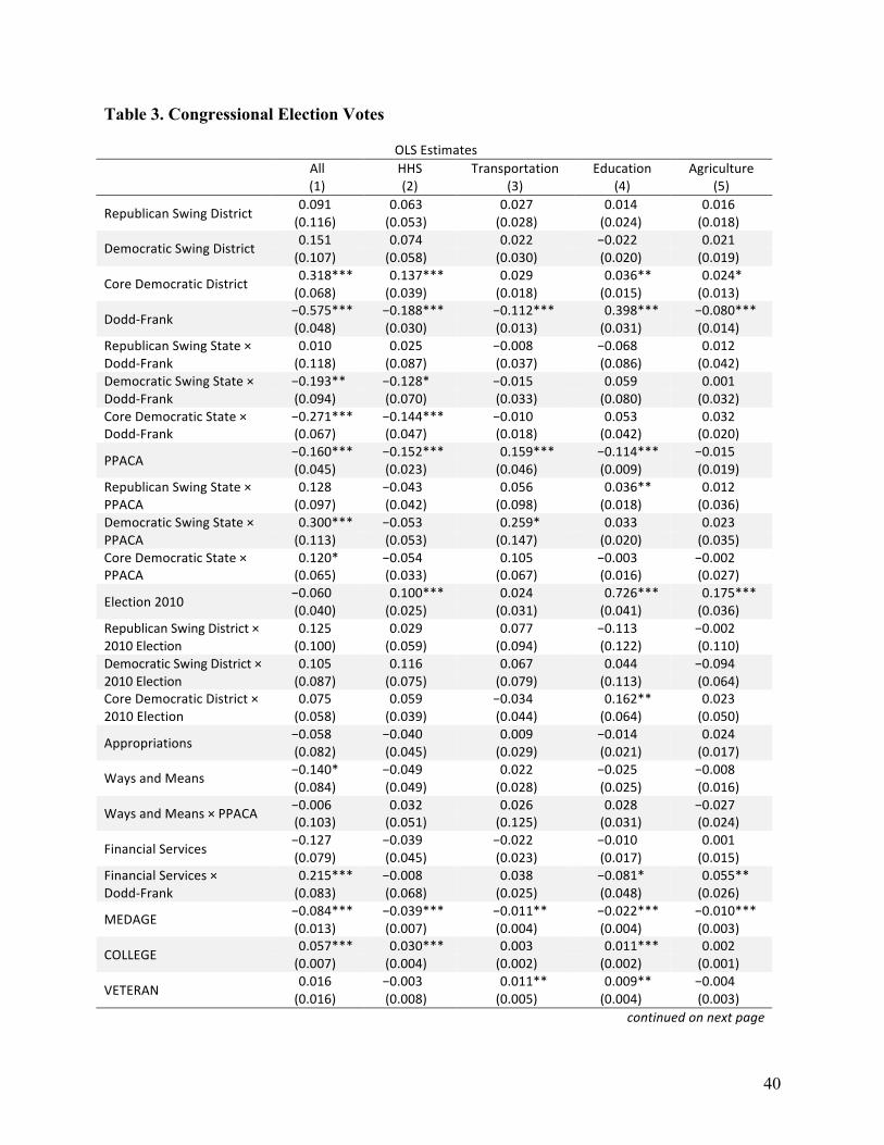
40

Table 3. Congressional Election Votes

OLS  Estimates  

 All  (1)  

HHS  (2)  

Transportation  (3)  

Education  (4)  

Agriculture  (5)  

Republican  Swing  District  0.091   0.063   0.027   0.014   0.016  (0.116)   (0.053)   (0.028)   (0.024)   (0.018)  

Democratic  Swing  District   0.151   0.074   0.022   −0.022   0.021  (0.107)   (0.058)   (0.030)   (0.020)   (0.019)  

Core  Democratic  District   0.318***   0.137***   0.029   0.036**   0.024*  (0.068)   (0.039)   (0.018)   (0.015)   (0.013)  

Dodd-­‐Frank  −0.575***   −0.188***   −0.112***   0.398***   −0.080***  (0.048)   (0.030)   (0.013)   (0.031)   (0.014)  

Republican  Swing  State  ×  Dodd-­‐Frank  

0.010   0.025   −0.008   −0.068   0.012  (0.118)   (0.087)   (0.037)   (0.086)   (0.042)  

Democratic  Swing  State  ×  Dodd-­‐Frank  

−0.193**   −0.128*   −0.015   0.059   0.001  (0.094)   (0.070)   (0.033)   (0.080)   (0.032)  

Core  Democratic  State  ×  Dodd-­‐Frank  

−0.271***   −0.144***   −0.010   0.053   0.032  (0.067)   (0.047)   (0.018)   (0.042)   (0.020)  

PPACA  −0.160***   −0.152***   0.159***   −0.114***   −0.015  (0.045)   (0.023)   (0.046)   (0.009)   (0.019)  

Republican  Swing  State  ×  PPACA  

0.128   −0.043   0.056   0.036**   0.012  (0.097)   (0.042)   (0.098)   (0.018)   (0.036)  

Democratic  Swing  State  ×  PPACA  

0.300***   −0.053   0.259*   0.033   0.023  (0.113)   (0.053)   (0.147)   (0.020)   (0.035)  

Core  Democratic  State  ×  PPACA  

0.120*   −0.054   0.105   −0.003   −0.002  (0.065)   (0.033)   (0.067)   (0.016)   (0.027)  

Election  2010  −0.060   0.100***   0.024   0.726***   0.175***  (0.040)   (0.025)   (0.031)   (0.041)   (0.036)  

Republican  Swing  District  ×  2010  Election  

0.125   0.029   0.077   −0.113   −0.002  (0.100)   (0.059)   (0.094)   (0.122)   (0.110)  

Democratic  Swing  District  ×  2010  Election  

0.105   0.116   0.067   0.044   −0.094  (0.087)   (0.075)   (0.079)   (0.113)   (0.064)  

Core  Democratic  District  ×  2010  Election  

0.075   0.059   −0.034   0.162**   0.023  (0.058)   (0.039)   (0.044)   (0.064)   (0.050)  

Appropriations  −0.058   −0.040   0.009   −0.014   0.024  (0.082)   (0.045)   (0.029)   (0.021)   (0.017)  

Ways  and  Means   −0.140*   −0.049   0.022   −0.025   −0.008  (0.084)   (0.049)   (0.028)   (0.025)   (0.016)  

Ways  and  Means  ×  PPACA   −0.006   0.032   0.026   0.028   −0.027  (0.103)   (0.051)   (0.125)   (0.031)   (0.024)  

Financial  Services  −0.127   −0.039   −0.022   −0.010   0.001  (0.079)   (0.045)   (0.023)   (0.017)   (0.015)  

Financial  Services  ×    Dodd-­‐Frank  

0.215***   −0.008   0.038   −0.081*   0.055**  (0.083)   (0.068)   (0.025)   (0.048)   (0.026)  

MEDAGE   −0.084***   −0.039***   −0.011**   −0.022***   −0.010***  (0.013)   (0.007)   (0.004)   (0.004)   (0.003)  

COLLEGE  0.057***   0.030***   0.003   0.011***   0.002  (0.007)   (0.004)   (0.002)   (0.002)   (0.001)  

VETERAN  0.016   −0.003   0.011**   0.009**   −0.004  (0.016)   (0.008)   (0.005)   (0.004)   (0.003)  

        continued  on  next  page  

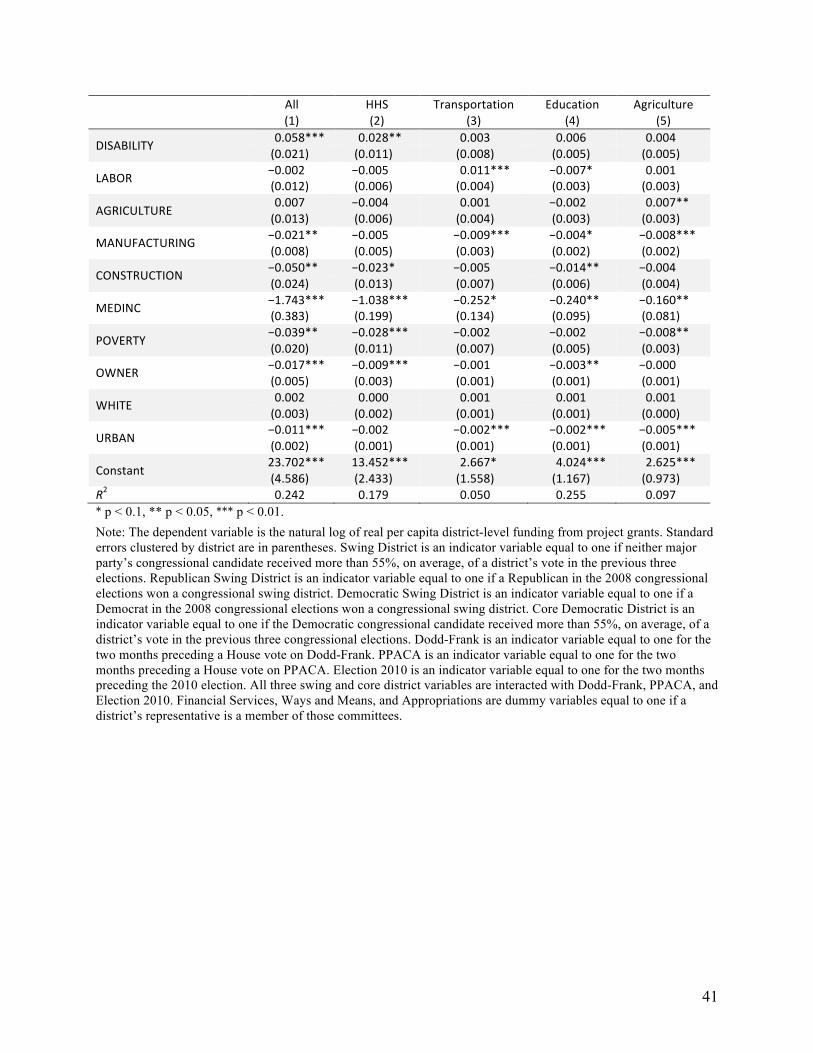
41

 All  (1)  

HHS  (2)  

Transportation  (3)  

Education  (4)  

Agriculture  (5)  

DISABILITY   0.058***   0.028**   0.003   0.006   0.004  (0.021)   (0.011)   (0.008)   (0.005)   (0.005)  

LABOR   −0.002   −0.005   0.011***   −0.007*   0.001  (0.012)   (0.006)   (0.004)   (0.003)   (0.003)  

AGRICULTURE  0.007   −0.004   0.001   −0.002   0.007**  (0.013)   (0.006)   (0.004)   (0.003)   (0.003)  

MANUFACTURING   −0.021**   −0.005   −0.009***   −0.004*   −0.008***  (0.008)   (0.005)   (0.003)   (0.002)   (0.002)  

CONSTRUCTION   −0.050**   −0.023*   −0.005   −0.014**   −0.004  (0.024)   (0.013)   (0.007)   (0.006)   (0.004)  

MEDINC   −1.743***   −1.038***   −0.252*   −0.240**   −0.160**  (0.383)   (0.199)   (0.134)   (0.095)   (0.081)  

POVERTY  −0.039**   −0.028***   −0.002   −0.002   −0.008**  (0.020)   (0.011)   (0.007)   (0.005)   (0.003)  

OWNER   −0.017***   −0.009***   −0.001   −0.003**   −0.000  (0.005)   (0.003)   (0.001)   (0.001)   (0.001)  

WHITE   0.002   0.000   0.001   0.001   0.001  (0.003)   (0.002)   (0.001)   (0.001)   (0.000)  

URBAN  −0.011***   −0.002   −0.002***   −0.002***   −0.005***  (0.002)   (0.001)   (0.001)   (0.001)   (0.001)  

Constant  23.702***   13.452***   2.667*   4.024***   2.625***  (4.586)   (2.433)   (1.558)   (1.167)   (0.973)  

R2   0.242   0.179   0.050   0.255   0.097  * p < 0.1, ** p < 0.05, *** p < 0.01. Note: The dependent variable is the natural log of real per capita district-level funding from project grants. Standard errors clustered by district are in parentheses. Swing District is an indicator variable equal to one if neither major party’s congressional candidate received more than 55%, on average, of a district’s vote in the previous three elections. Republican Swing District is an indicator variable equal to one if a Republican in the 2008 congressional elections won a congressional swing district. Democratic Swing District is an indicator variable equal to one if a Democrat in the 2008 congressional elections won a congressional swing district. Core Democratic District is an indicator variable equal to one if the Democratic congressional candidate received more than 55%, on average, of a district’s vote in the previous three congressional elections. Dodd-Frank is an indicator variable equal to one for the two months preceding a House vote on Dodd-Frank. PPACA is an indicator variable equal to one for the two months preceding a House vote on PPACA. Election 2010 is an indicator variable equal to one for the two months preceding the 2010 election. All three swing and core district variables are interacted with Dodd-Frank, PPACA, and Election 2010. Financial Services, Ways and Means, and Appropriations are dummy variables equal to one if a district’s representative is a member of those committees.

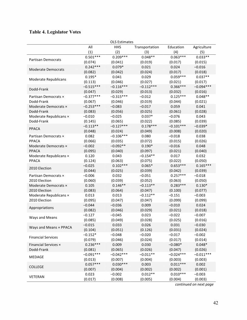
42

Table 4. Legislator Votes

OLS  Estimates  

 All  (1)  

HHS  (2)  

Transportation  (3)  

Education  (4)  

Agriculture  (5)  

Partisan  Democrats  0.501***   0.209***   0.048**   0.063***   0.033**  (0.074)   (0.041)   (0.019)   (0.017)   (0.015)  

Moderate  Democrats   0.242***   0.079*   0.021   0.024   −0.016  (0.082)   (0.042)   (0.024)   (0.017)   (0.018)  

Moderate  Republicans   0.195*   0.041   0.029   0.059***   0.037**  (0.113)   (0.046)   (0.027)   (0.021)   (0.017)  

Dodd-­‐Frank  −0.515***   −0.116***   −0.112***   0.366***   −0.094***  (0.047)   (0.029)   (0.013)   (0.032)   (0.016)  

Partisan  Democrats  ×  Dodd-­‐Frank  

−0.377***   −0.315***   −0.012   0.125***   0.048**  (0.067)   (0.046)   (0.019)   (0.044)   (0.021)  

Moderate  Democrats  ×  Dodd-­‐Frank  

−0.253***   −0.083   −0.017   0.059   0.041  (0.083)   (0.056)   (0.025)   (0.061)   (0.028)  

Moderate  Republicans  ×  Dodd-­‐Frank  

−0.010   −0.025   0.037*   −0.076   0.043  (0.145)   (0.065)   (0.022)   (0.085)   (0.039)  

PPACA  −0.113**   −0.127***   0.178***   −0.101***   −0.039*  (0.048)   (0.024)   (0.049)   (0.008)   (0.020)  

Partisan  Democrats  ×  PPACA  

0.082   −0.106***   0.080   −0.018   0.038  (0.066)   (0.035)   (0.072)   (0.015)   (0.026)  

Moderate  Democrats  ×  PPACA  

−0.002   −0.092**   0.190*   −0.016   0.048  (0.095)   (0.040)   (0.097)   (0.021)   (0.040)  

Moderate  Republicans  ×  PPACA  

0.120   0.043   −0.154**   0.017   0.032  (0.124)   (0.063)   (0.075)   (0.022)   (0.050)  

2010  Election  −0.025   0.102***   0.065*   0.653***   0.165***  (0.044)   (0.025)   (0.039)   (0.042)   (0.039)  

Partisan  Democrats  ×    2010  Election  

−0.006   0.032   −0.051   0.257***   −0.018  (0.060)   (0.039)   (0.052)   (0.063)   (0.050)  

Moderate  Democrats  ×  2010  Election  

0.105   0.146**   −0.113**   0.283***   0.130*  (0.083)   (0.064)   (0.047)   (0.100)   (0.077)  

Moderate  Republicans  ×  2010  Election  

0.013   0.013   −0.112**   −0.151   −0.003  (0.095)   (0.047)   (0.047)   (0.099)   (0.099)  

Appropriations  −0.044   −0.036   0.009   −0.010   0.024  (0.082)   (0.046)   (0.029)   (0.021)   (0.018)  

Ways  and  Means   −0.127   −0.045   0.023   −0.022   −0.007  (0.085)   (0.049)   (0.028)   (0.025)   (0.016)  

Ways  and  Means  ×  PPACA   −0.015   0.033   0.026   0.031   −0.030  (0.104)   (0.051)   (0.126)   (0.031)   (0.024)  

Financial  Services  −0.152*   −0.048   −0.020   −0.017   −0.002  (0.079)   (0.046)   (0.024)   (0.017)   (0.014)  

Financial  Services  ×    Dodd-­‐Frank  

0.236***   0.009   0.030   −0.080*   0.048*  (0.081)   (0.065)   (0.026)   (0.047)   (0.026)  

MEDAGE   −0.091***   −0.042***   −0.011**   −0.024***   −0.011***  (0.013)   (0.007)   (0.004)   (0.003)   (0.003)  

COLLEGE  0.057***   0.030***   0.003   0.011***   0.002  (0.007)   (0.004)   (0.002)   (0.002)   (0.001)  

VETERAN  0.023   −0.002   0.012**   0.010***   −0.003  (0.017)   (0.008)   (0.005)   (0.004)   (0.003)  

        continued  on  next  page  

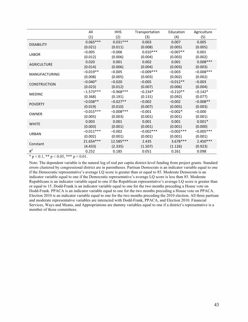
43

 All  (1)  

HHS  (2)  

Transportation  (3)  

Education  (4)  

Agriculture  (5)  

DISABILITY   0.065***   0.031***   0.003   0.007   0.005  (0.021)   (0.011)   (0.008)   (0.005)   (0.005)  

LABOR   −0.005   −0.006   0.010***   −0.007**   0.001  (0.012)   (0.006)   (0.004)   (0.003)   (0.002)  

AGRICULTURE  0.020   0.001   0.002   0.001   0.008***  (0.014)   (0.006)   (0.004)   (0.003)   (0.003)  

MANUFACTURING   −0.019**   −0.005   −0.009***   −0.003   −0.008***  (0.008)   (0.005)   (0.003)   (0.002)   (0.002)  

CONSTRUCTION   −0.040*   −0.020   −0.005   −0.012**   −0.003  (0.023)   (0.012)   (0.007)   (0.006)   (0.004)  

MEDINC   −1.573***   −0.968***   −0.234*   −0.210**   −0.142*  (0.368)   (0.191)   (0.131)   (0.092)   (0.077)  

POVERTY  −0.038**   −0.027**   −0.002   −0.002   −0.008**  (0.019)   (0.010)   (0.007)   (0.005)   (0.003)  

OWNER   −0.015***   −0.008***   −0.001   −0.002*   −0.000  (0.005)   (0.003)   (0.001)   (0.001)   (0.001)  

WHITE   0.003   0.001   0.001   0.001   0.001*  (0.003)   (0.001)   (0.001)   (0.001)   (0.000)  

URBAN  −0.011***   −0.002   −0.002***   −0.002***   −0.005***  (0.002)   (0.001)   (0.001)   (0.001)   (0.001)  

Constant  21.654***   12.585***   2.435   3.678***   2.450***  (4.433)   (2.335)   (1.507)   (1.126)   (0.923)  

R2   0.252   0.185   0.051   0.261   0.098  * p < 0.1, ** p < 0.05, *** p < 0.01. Note: The dependent variable is the natural log of real per capita district-level funding from project grants. Standard errors clustered by congressional district are in parentheses. Partisan Democrats is an indicator variable equal to one if the Democratic representative’s average LQ score is greater than or equal to 85. Moderate Democrats is an indicator variable equal to one if the Democratic representative’s average LQ score is less than 85. Moderate Republicans is an indicator variable equal to one if the Republican representative’s average LQ score is greater than or equal to 15. Dodd-Frank is an indicator variable equal to one for the two months preceding a House vote on Dodd-Frank. PPACA is an indicator variable equal to one for the two months preceding a House vote on PPACA. Election 2010 is an indicator variable equal to one for the two months preceding the 2010 election. All three partisan and moderate representative variables are interacted with Dodd-Frank, PPACA, and Election 2010. Financial Services, Ways and Means, and Appropriations are dummy variables equal to one if a district’s representative is a member of those committees.

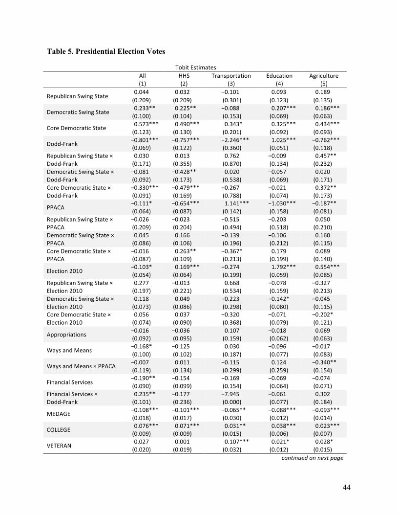
44

Table 5. Presidential Election Votes

Tobit  Estimates  

All  (1)  

HHS  (2)  

Transportation  (3)  

Education  (4)  

Agriculture  (5)  

Republican  Swing  State  0.044   0.032   −0.101   0.093   0.189  (0.209)   (0.209)   (0.301)   (0.123)   (0.135)  

Democratic  Swing  State   0.233**   0.225**   −0.088   0.207***   0.186***  (0.100)   (0.104)   (0.153)   (0.069)   (0.063)  

Core  Democratic  State   0.573***   0.490***   0.343*   0.325***   0.434***  (0.123)   (0.130)   (0.201)   (0.092)   (0.093)  

Dodd-­‐Frank   −0.801***   −0.757***   −2.246***   1.025***   −0.762***  (0.069)   (0.122)   (0.360)   (0.051)   (0.118)  

Republican  Swing  State  ×  Dodd-­‐Frank  

0.030   0.013   0.762   −0.009   0.457**  (0.171)   (0.355)   (0.870)   (0.134)   (0.232)  

Democratic  Swing  State  ×  Dodd-­‐Frank  

−0.081   −0.428**   0.020   −0.057   0.020  (0.092)   (0.173)   (0.538)   (0.069)   (0.171)  

Core  Democratic  State  ×  Dodd-­‐Frank  

−0.330***   −0.479***   −0.267   −0.021   0.372**  (0.091)   (0.169)   (0.788)   (0.074)   (0.173)  

PPACA  −0.111*   −0.654***   1.141***   −1.030***   −0.187**  (0.064)   (0.087)   (0.142)   (0.158)   (0.081)  

Republican  Swing  State  ×  PPACA  

−0.026   −0.023   −0.515   −0.203   0.050  (0.209)   (0.204)   (0.494)   (0.518)   (0.210)  

Democratic  Swing  State  ×  PPACA  

0.045   0.166   −0.139   −0.106   0.160  (0.086)   (0.106)   (0.196)   (0.212)   (0.115)  

Core  Democratic  State  ×  PPACA  

−0.016   0.263**   −0.367*   0.179   0.089  (0.087)   (0.109)   (0.213)   (0.199)   (0.140)  

Election  2010  −0.103*   0.169***   −0.274   1.792***   0.554***  (0.054)   (0.064)   (0.199)   (0.059)   (0.085)  

Republican  Swing  State  ×  Election  2010  

0.277   −0.013   0.668   −0.078   −0.327  (0.197)   (0.221)   (0.534)   (0.159)   (0.213)  

Democratic  Swing  State  ×  Election  2010  

0.118   0.049   −0.223   −0.142*   −0.045  (0.073)   (0.086)   (0.298)   (0.080)   (0.115)  

Core  Democratic  State  ×  Election  2010  

0.056   0.037   −0.320   −0.071   −0.202*  (0.074)   (0.090)   (0.368)   (0.079)   (0.121)  

Appropriations  −0.016   −0.036   0.107   −0.018   0.069  (0.092)   (0.095)   (0.159)   (0.062)   (0.063)  

Ways  and  Means   −0.168*   −0.125   0.030   −0.096   −0.017  (0.100)   (0.102)   (0.187)   (0.077)   (0.083)  

Ways  and  Means  ×  PPACA   −0.007   0.011   −0.115   0.124   −0.340**  (0.119)   (0.134)   (0.299)   (0.259)   (0.154)  

Financial  Services  −0.190**   −0.154   −0.169   −0.069   −0.074  (0.090)   (0.099)   (0.154)   (0.064)   (0.071)  

Financial  Services  ×    Dodd-­‐Frank  

0.235**   −0.177   −7.945   −0.061   0.302  (0.101)   (0.236)   (0.000)   (0.077)   (0.184)  

MEDAGE   −0.108***   −0.101***   −0.065**   −0.088***   −0.093***  (0.018)   (0.017)   (0.030)   (0.012)   (0.014)  

COLLEGE   0.076***   0.071***   0.031**   0.038***   0.023***  (0.009)   (0.009)   (0.015)   (0.006)   (0.007)  

VETERAN  0.027   0.001   0.107***   0.021*   0.028*  (0.020)   (0.019)   (0.032)   (0.012)   (0.015)  

        continued  on  next  page  

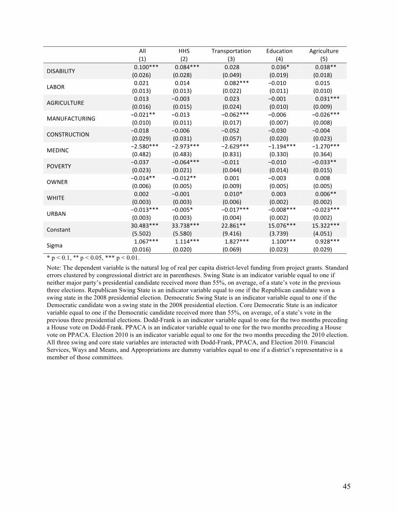
45

 All  (1)  

HHS  (2)  

Transportation  (3)  

Education  (4)  

Agriculture  (5)  

DISABILITY   0.100***   0.084***   0.028   0.036*   0.038**  (0.026)   (0.028)   (0.049)   (0.019)   (0.018)  

LABOR   0.021   0.014   0.082***   −0.010   0.015  (0.013)   (0.013)   (0.022)   (0.011)   (0.010)  

AGRICULTURE  0.013   −0.003   0.023   −0.001   0.031***  (0.016)   (0.015)   (0.024)   (0.010)   (0.009)  

MANUFACTURING   −0.021**   −0.013   −0.062***   −0.006   −0.026***  (0.010)   (0.011)   (0.017)   (0.007)   (0.008)  

CONSTRUCTION   −0.018   −0.006   −0.052   −0.030   −0.004  (0.029)   (0.031)   (0.057)   (0.020)   (0.023)  

MEDINC   −2.580***   −2.973***   −2.629***   −1.194***   −1.270***  (0.482)   (0.483)   (0.831)   (0.330)   (0.364)  

POVERTY  −0.037   −0.064***   −0.011   −0.010   −0.033**  (0.023)   (0.021)   (0.044)   (0.014)   (0.015)  

OWNER   −0.014**   −0.012**   0.001   −0.003   0.008  (0.006)   (0.005)   (0.009)   (0.005)   (0.005)  

WHITE   0.002   −0.001   0.010*   0.003   0.006**  (0.003)   (0.003)   (0.006)   (0.002)   (0.002)  

URBAN  −0.013***   −0.005*   −0.017***   −0.008***   −0.023***  (0.003)   (0.003)   (0.004)   (0.002)   (0.002)  

Constant  30.483***   33.738***   22.861**   15.076***   15.322***  (5.502)   (5.580)   (9.416)   (3.739)   (4.051)  

Sigma   1.067***   1.114***   1.827***   1.100***   0.928***  (0.016)   (0.020)   (0.069)   (0.023)   (0.029)  

* p < 0.1, ** p < 0.05, *** p < 0.01. Note: The dependent variable is the natural log of real per capita district-level funding from project grants. Standard errors clustered by congressional district are in parentheses. Swing State is an indicator variable equal to one if neither major party’s presidential candidate received more than 55%, on average, of a state’s vote in the previous three elections. Republican Swing State is an indicator variable equal to one if the Republican candidate won a swing state in the 2008 presidential election. Democratic Swing State is an indicator variable equal to one if the Democratic candidate won a swing state in the 2008 presidential election. Core Democratic State is an indicator variable equal to one if the Democratic candidate received more than 55%, on average, of a state’s vote in the previous three presidential elections. Dodd-Frank is an indicator variable equal to one for the two months preceding a House vote on Dodd-Frank. PPACA is an indicator variable equal to one for the two months preceding a House vote on PPACA. Election 2010 is an indicator variable equal to one for the two months preceding the 2010 election. All three swing and core state variables are interacted with Dodd-Frank, PPACA, and Election 2010. Financial Services, Ways and Means, and Appropriations are dummy variables equal to one if a district’s representative is a member of those committees.

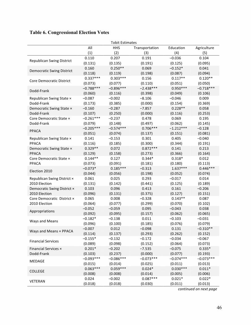
46

Table 6. Congressional Election Votes

Tobit  Estimates  

All  (1)  

HHS  (2)  

Transportation  (3)  

Education  (4)  

Agriculture  (5)  

Republican  Swing  District  0.110   0.207   0.191   −0.036   0.104  (0.131)   (0.135)   (0.191)   (0.125)   (0.095)  

Democratic  Swing  District   0.160   0.250**   0.069   −0.152*   0.041  (0.118)   (0.119)   (0.198)   (0.087)   (0.094)  

Core  Democratic  District   0.337***   0.303***   0.156   0.117**   0.120**  (0.073)   (0.077)   (0.110)   (0.051)   (0.050)  

Dodd-­‐Frank   −0.788***   −0.896***   −2.438***   0.950***   −0.718***  (0.060)   (0.116)   (0.398)   (0.049)   (0.106)  

Republican  Swing  State  ×  Dodd-­‐Frank  

−0.087   −0.002   −8.106   −0.046   0.009  (0.173)   (0.385)   (0.000)   (0.154)   (0.369)  

Democratic  Swing  State  ×  Dodd-­‐Frank  

−0.160   −0.287   −7.857   0.228**   0.058  (0.107)   (0.250)   (0.000)   (0.116)   (0.253)  

Core  Democratic  State  ×  Dodd-­‐Frank  

−0.261***   −0.237   0.478   0.069   0.195  (0.079)   (0.148)   (0.497)   (0.062)   (0.145)  

PPACA  −0.205***   −0.574***   0.706***   −1.212***   −0.128  (0.051)   (0.074)   (0.137)   (0.151)   (0.081)  

Republican  Swing  State  ×  PPACA  

0.141   −0.153   0.301   0.405   −0.040  (0.116)   (0.185)   (0.300)   (0.344)   (0.191)  

Democratic  Swing  State  ×  PPACA  

0.329**   0.072   0.872***   0.141   0.213  (0.129)   (0.158)   (0.273)   (0.366)   (0.164)  

Core  Democratic  State  ×  PPACA  

0.144**   0.127   0.344*   0.318*   0.012  (0.073)   (0.091)   (0.181)   (0.180)   (0.113)  

Election  2010  −0.073*   0.185***   −0.313   1.637***   0.446***  (0.044)   (0.056)   (0.198)   (0.052)   (0.074)  

Republican  Swing  District  ×  2010  Election  

0.061   0.025   0.293   −0.017   0.014  (0.131)   (0.142)   (0.441)   (0.125)   (0.189)  

Democratic  Swing  District  ×  2010  Election  

0.103   0.096   0.413   0.161   −0.206  (0.096)   (0.131)   (0.375)   (0.127)   (0.151)  

Core  Democratic    District  ×  2010  Election  

0.065   0.008   −0.328   0.143**   0.087  (0.064)   (0.077)   (0.299)   (0.070)   (0.102)  

Appropriations  −0.052   −0.059   0.095   −0.043   0.038  (0.092)   (0.095)   (0.157)   (0.062)   (0.065)  

Ways  and  Means   −0.182*   −0.138   0.011   −0.103   −0.031  (0.096)   (0.100)   (0.185)   (0.076)   (0.079)  

Ways  and  Means  ×  PPACA   −0.007   0.012   −0.098   0.131   −0.310**  (0.114)   (0.137)   (0.293)   (0.262)   (0.152)  

Financial  Services  −0.155*   −0.132   −0.172   −0.034   −0.067  (0.089)   (0.098)   (0.152)   (0.064)   (0.073)  

Financial  Services  ×    Dodd-­‐Frank  

0.201*   −0.202   −7.535   −0.075   0.335*  (0.103)   (0.237)   (0.000)   (0.077)   (0.193)  

MEDAGE   −0.093***   −0.086***   −0.073***   −0.074***   −0.073***  (0.015)   (0.014)   (0.025)   (0.011)   (0.013)  

COLLEGE   0.063***   0.059***   0.024*   0.030***   0.011*  (0.008)   (0.008)   (0.014)   (0.005)   (0.006)  

VETERAN  0.024   −0.002   0.087***   0.021*   0.022*  (0.018)   (0.018)   (0.030)   (0.011)   (0.013)  

        continued  on  next  page  

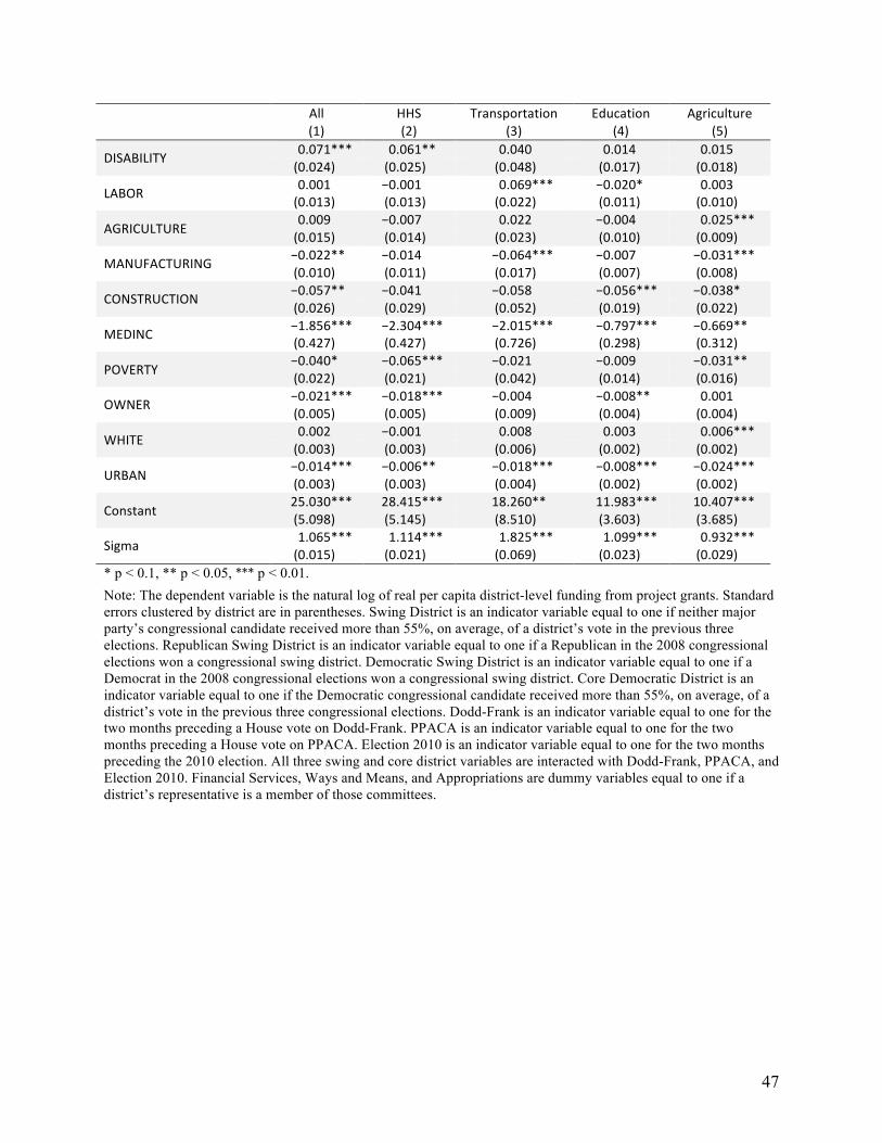
47

 All  (1)  

HHS  (2)  

Transportation  (3)  

Education  (4)  

Agriculture  (5)  

DISABILITY   0.071***   0.061**   0.040   0.014   0.015  (0.024)   (0.025)   (0.048)   (0.017)   (0.018)  

LABOR   0.001   −0.001   0.069***   −0.020*   0.003  (0.013)   (0.013)   (0.022)   (0.011)   (0.010)  

AGRICULTURE  0.009   −0.007   0.022   −0.004   0.025***  (0.015)   (0.014)   (0.023)   (0.010)   (0.009)  

MANUFACTURING   −0.022**   −0.014   −0.064***   −0.007   −0.031***  (0.010)   (0.011)   (0.017)   (0.007)   (0.008)  

CONSTRUCTION   −0.057**   −0.041   −0.058   −0.056***   −0.038*  (0.026)   (0.029)   (0.052)   (0.019)   (0.022)  

MEDINC   −1.856***   −2.304***   −2.015***   −0.797***   −0.669**  (0.427)   (0.427)   (0.726)   (0.298)   (0.312)  

POVERTY  −0.040*   −0.065***   −0.021   −0.009   −0.031**  (0.022)   (0.021)   (0.042)   (0.014)   (0.016)  

OWNER   −0.021***   −0.018***   −0.004   −0.008**   0.001  (0.005)   (0.005)   (0.009)   (0.004)   (0.004)  

WHITE   0.002   −0.001   0.008   0.003   0.006***  (0.003)   (0.003)   (0.006)   (0.002)   (0.002)  

URBAN  −0.014***   −0.006**   −0.018***   −0.008***   −0.024***  (0.003)   (0.003)   (0.004)   (0.002)   (0.002)  

Constant  25.030***   28.415***   18.260**   11.983***   10.407***  (5.098)   (5.145)   (8.510)   (3.603)   (3.685)  

Sigma   1.065***   1.114***   1.825***   1.099***   0.932***  (0.015)   (0.021)   (0.069)   (0.023)   (0.029)  

* p < 0.1, ** p < 0.05, *** p < 0.01. Note: The dependent variable is the natural log of real per capita district-level funding from project grants. Standard errors clustered by district are in parentheses. Swing District is an indicator variable equal to one if neither major party’s congressional candidate received more than 55%, on average, of a district’s vote in the previous three elections. Republican Swing District is an indicator variable equal to one if a Republican in the 2008 congressional elections won a congressional swing district. Democratic Swing District is an indicator variable equal to one if a Democrat in the 2008 congressional elections won a congressional swing district. Core Democratic District is an indicator variable equal to one if the Democratic congressional candidate received more than 55%, on average, of a district’s vote in the previous three congressional elections. Dodd-Frank is an indicator variable equal to one for the two months preceding a House vote on Dodd-Frank. PPACA is an indicator variable equal to one for the two months preceding a House vote on PPACA. Election 2010 is an indicator variable equal to one for the two months preceding the 2010 election. All three swing and core district variables are interacted with Dodd-Frank, PPACA, and Election 2010. Financial Services, Ways and Means, and Appropriations are dummy variables equal to one if a district’s representative is a member of those committees.

48

Table 7. Legislators’ Votes

Tobit  Estimates  

All  (1)  

HHS  (2)  

Transportation  (3)  

Education  (4)  

Agriculture  (5)  

Partisan  Democrats  0.565***   0.512***   0.243*   0.274***   0.229***  (0.082)   (0.089)   (0.124)   (0.061)   (0.061)  

Moderate  Democrats   0.254***   0.214**   0.164   0.119*   0.040  (0.091)   (0.095)   (0.145)   (0.066)   (0.061)  

Moderate  Republicans   0.235*   0.071   0.339   0.127   0.243**  (0.134)   (0.130)   (0.235)   (0.094)   (0.108)  

Dodd-­‐Frank  −0.734***   −0.662***   −2.742***   0.977***   −0.782***  (0.062)   (0.113)   (0.454)   (0.053)   (0.120)  

Partisan  Democrats  ×  Dodd-­‐Frank  

−0.342***   −0.677***   0.757   0.062   0.200  (0.081)   (0.146)   (0.583)   (0.068)   (0.171)  

Moderate  Democrats  ×  Dodd-­‐Frank  

−0.227**   −0.269   0.753   −0.016   0.356**  (0.101)   (0.207)   (0.612)   (0.087)   (0.158)  

Moderate  Republicans  ×  Dodd-­‐Frank  

−0.191   −0.462   −7.066   −0.088   0.125  (0.208)   (0.458)   (0.000)   (0.135)   (0.385)  

PPACA  −0.145***   −0.576***   0.778***   −1.294***   −0.182**  (0.055)   (0.088)   (0.142)   (0.180)   (0.086)  

Partisan  Democrats  ×  PPACA  

0.102   0.130   0.260   0.454**   0.125  (0.074)   (0.101)   (0.192)   (0.204)   (0.121)  

Moderate  Democrats  ×  PPACA  

0.018   −0.020   0.576***   0.197   0.204  (0.104)   (0.124)   (0.215)   (0.282)   (0.131)  

Moderate  Republicans  ×  PPACA  

−0.048   0.071   −0.615   0.118   −0.198  (0.185)   (0.258)   (0.401)   (0.491)   (0.268)  

2010  Election  −0.040   0.178***   −0.128   1.606***   0.410***  (0.051)   (0.058)   (0.200)   (0.054)   (0.078)  

Partisan  Democrats  ×    2010  Election  

−0.019   −0.055   −0.227   0.191***   0.084  (0.067)   (0.077)   (0.294)   (0.071)   (0.107)  

Moderate  Democrats  ×  2010  Election  

0.105   0.223*   −0.734**   0.214**   0.156  (0.092)   (0.114)   (0.329)   (0.102)   (0.134)  

Moderate  Republicans  ×  2010  Election  

0.012   0.207   −1.447*   −0.185   −0.012  (0.112)   (0.131)   (0.813)   (0.148)   (0.221)  

Appropriations  −0.040   −0.053   0.116   −0.033   0.048  (0.091)   (0.095)   (0.159)   (0.061)   (0.067)  

Ways  and  Means   −0.170*   −0.132   0.023   −0.096   −0.027  (0.096)   (0.098)   (0.185)   (0.077)   (0.082)  

Ways  and  Means  ×  PPACA   −0.022   −0.005   −0.088   0.100   −0.336**  (0.116)   (0.138)   (0.299)   (0.267)   (0.155)  

Financial  Services  −0.181**   −0.150   −0.173   −0.064   −0.087  (0.088)   (0.097)   (0.153)   (0.064)   (0.071)  

Financial  Services  ×    Dodd-­‐Frank  

0.234**   −0.142   −7.566   −0.058   0.315*  (0.103)   (0.228)   (0.000)   (0.078)   (0.187)  

MEDAGE   −0.103***   −0.094***   −0.077***   −0.082***   −0.083***  (0.015)   (0.015)   (0.026)   (0.011)   (0.014)  

COLLEGE  0.064***   0.060***   0.023*   0.030***   0.012**  (0.008)   (0.008)   (0.014)   (0.005)   (0.006)  

VETERAN  0.032   0.003   0.091***   0.025**   0.028**  (0.020)   (0.019)   (0.031)   (0.011)   (0.013)  

        continued  on  next  page  

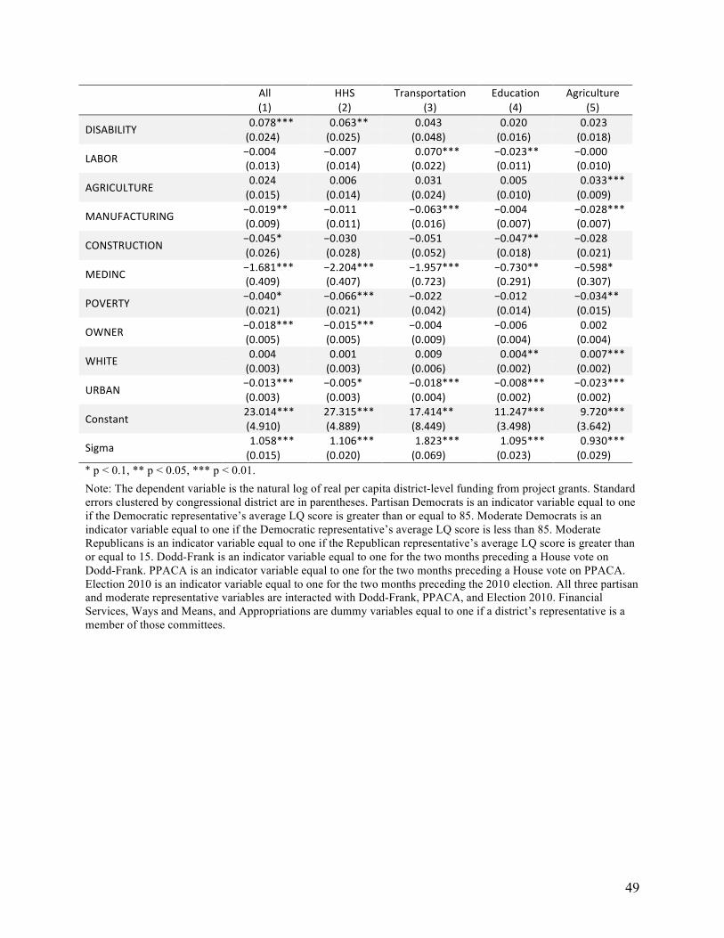
49

 All  (1)  

HHS  (2)  

Transportation  (3)  

Education  (4)  

Agriculture  (5)  

DISABILITY   0.078***   0.063**   0.043   0.020   0.023  (0.024)   (0.025)   (0.048)   (0.016)   (0.018)  

LABOR   −0.004   −0.007   0.070***   −0.023**   −0.000  (0.013)   (0.014)   (0.022)   (0.011)   (0.010)  

AGRICULTURE  0.024   0.006   0.031   0.005   0.033***  (0.015)   (0.014)   (0.024)   (0.010)   (0.009)  

MANUFACTURING   −0.019**   −0.011   −0.063***   −0.004   −0.028***  (0.009)   (0.011)   (0.016)   (0.007)   (0.007)  

CONSTRUCTION   −0.045*   −0.030   −0.051   −0.047**   −0.028  (0.026)   (0.028)   (0.052)   (0.018)   (0.021)  

MEDINC   −1.681***   −2.204***   −1.957***   −0.730**   −0.598*  (0.409)   (0.407)   (0.723)   (0.291)   (0.307)  

POVERTY  −0.040*   −0.066***   −0.022   −0.012   −0.034**  (0.021)   (0.021)   (0.042)   (0.014)   (0.015)  

OWNER   −0.018***   −0.015***   −0.004   −0.006   0.002  (0.005)   (0.005)   (0.009)   (0.004)   (0.004)  

WHITE   0.004   0.001   0.009   0.004**   0.007***  (0.003)   (0.003)   (0.006)   (0.002)   (0.002)  

URBAN  −0.013***   −0.005*   −0.018***   −0.008***   −0.023***  (0.003)   (0.003)   (0.004)   (0.002)   (0.002)  

Constant  23.014***   27.315***   17.414**   11.247***   9.720***  (4.910)   (4.889)   (8.449)   (3.498)   (3.642)  

Sigma   1.058***   1.106***   1.823***   1.095***   0.930***  (0.015)   (0.020)   (0.069)   (0.023)   (0.029)  

* p < 0.1, ** p < 0.05, *** p < 0.01. Note: The dependent variable is the natural log of real per capita district-level funding from project grants. Standard errors clustered by congressional district are in parentheses. Partisan Democrats is an indicator variable equal to one if the Democratic representative’s average LQ score is greater than or equal to 85. Moderate Democrats is an indicator variable equal to one if the Democratic representative’s average LQ score is less than 85. Moderate Republicans is an indicator variable equal to one if the Republican representative’s average LQ score is greater than or equal to 15. Dodd-Frank is an indicator variable equal to one for the two months preceding a House vote on Dodd-Frank. PPACA is an indicator variable equal to one for the two months preceding a House vote on PPACA. Election 2010 is an indicator variable equal to one for the two months preceding the 2010 election. All three partisan and moderate representative variables are interacted with Dodd-Frank, PPACA, and Election 2010. Financial Services, Ways and Means, and Appropriations are dummy variables equal to one if a district’s representative is a member of those committees.