PROBABILISTIC CORTICAL AND MYOCARDIAL FIBER

TRACKING IN DIFFUSION TENSOR IMAGING

by

Rakesh M. Lal

A thesis submitted to The Johns Hopkins University in conformity with the requirements

for the degree of Master of Science in Engineering

Baltimore, Maryland

February, 2004

c© Rakesh M. Lal 2004

All rights reserved

Abstract

This thesis involves the tracking of white matter and heart fibers, using diffusion ten-

sor imaging data and high resolution MR scans. Dynamic programming is employed

to generate fibers linking regions of interest in the brain and heart with paths that

minimize an energy constraint.

From the diffusion tensor data it is possible to determine the probability that

a fiber passing through a particular voxel is oriented in a particular direction. One

can define the energy associated with a path connecting a given voxel to one of its

neighboring voxels as the inverse of the probability of a fiber being oriented in the

direction of this neighbor. In addition assume this energy is additive. Thus the energy

associated with a path between two voxels and passing through a third voxel, is the

equal to the sum of the energies associated with the path from the starting voxel

to the intermediate voxel and the path from the intermediate voxel to the ending

voxel. Thus to determine the optimal path between a start and an end voxel, we

search over all paths connecting the two voxels and choose the path in which the

total energy is minimized. In order for this search to be performed more efficiently,

dynamic programming is used to reduce the complexity of the problem.

In addition a technique to extend the dynamic programming algorithm is

presented to take into account not only the diffusion tensor information, but also

accomodate any prior information about the Frenet characteristics of cortical and

myocardial fibers. Properties of average curvature and average torsion of the fibers

are incorporated into the cost function of the dynamic programming algorithm, so as

to better model fibers.

ii

Acknowledgements

I would like to express my deepest gratitude to my advisor, Dr. Michael I. Miller for all his

support and guidance during this project and for the exciting and challenging environment

he has provided for me. His enthusiasm and confidence in me has been a tremendous source

of inspiration. I am also indebted to my undergraduate advisor, Dr. Murray B. Sachs

who has always shown a vested interest in my success, and provided me with sound advice

whenever I needed it.

Special thanks to Dr. Susumu Mori and Dr. Xavier Golay, who were instrumental

in providing me with high quality data, and were always willing to share their knowledge

and expertise. I would also like to thank Allan Massie who assisted me in the development

and optimization of the algorithm. Also, I must thank Dr. Tilak Ratnanather for his

interest, guidance and advice in completing this project.

I would also like to thank my fellow students in the Center for Imaging Science with

whom I have been priviledged to work, for all the encouragement and discussion we shared.

I must thank those senior to me, particularly Faisal Beg, Cash Costello, and Paritosh Tyagi

for all their advice. In addition, Dmitri Bitouk, Marc Vaillant, Guang-Lih Huang, and

Srinivas Peddi have always provided a stimulating and intellectually rich environment. I

also appreciate all the friendships I formed at the center, with Jeff Homer, Raymond Hulse,

Aashish Majethia, Agatha Lee, Walter Barmak, Dawn Kilheffer, and Pam Lauria.

Finally, I would like to thank my parents and family for all their affection, encour-

agement and motivation to further my education. They have always shown a tremendous

amount of faith in me, and gave me the support and motivation I needed, and for this I am

eternally grateful.

Rakesh Lal

iii

Table of Contents

Page

List of Tables . . . . . . . . . . . . . . . . . . . . . . . . . . . . . . . . . . . . . . . . . . . . . . . . . . . . . . . . . . . . . . . . . . . . . . vi

List of Figures . . . . . . . . . . . . . . . . . . . . . . . . . . . . . . . . . . . . . . . . . . . . . . . . . . . . . . . . . . . . . . . . . . . . . vii

1 Introduction . . . . . . . . . . . . . . . . . . . . . . . . . . . . . . . . . . . . . . . . . . . . . . . . . . . . . . . . . . . . . . . . . . . . 1

1.1 Computational Anatomy . . . . . . . . . . . . . . . . . . . . . . . . . . . . . . . . . . . . . . . . . . . . . . 11.2 Tracking Fiber Projections . . . . . . . . . . . . . . . . . . . . . . . . . . . . . . . . . . . . . . . . . . . . 21.3 Thesis Layout . . . . . . . . . . . . . . . . . . . . . . . . . . . . . . . . . . . . . . . . . . . . . . . . . . . . . . . . 4

2 Methods and Algorithm . . . . . . . . . . . . . . . . . . . . . . . . . . . . . . . . . . . . . . . . . . . . . . . . . . . . . . 5

2.1 Diffusion Tensor Analysis . . . . . . . . . . . . . . . . . . . . . . . . . . . . . . . . . . . . . . . . . . . . . . 52.1.1 Conventional MRI . . . . . . . . . . . . . . . . . . . . . . . . . . . . . . . . . . . . . . . . . . . . . 52.1.2 Frequency Encoding and Slice Selection . . . . . . . . . . . . . . . . . . . . . . . . . . . 62.1.3 Phase Encoding and Fourier Transform Tomography . . . . . . . . . . . . . . . 62.1.4 T2 Weighed Imaging . . . . . . . . . . . . . . . . . . . . . . . . . . . . . . . . . . . . . . . . . . . . 72.1.5 Diffusion Tensor Imaging . . . . . . . . . . . . . . . . . . . . . . . . . . . . . . . . . . . . . . . 8

2.2 Dynamic Programming . . . . . . . . . . . . . . . . . . . . . . . . . . . . . . . . . . . . . . . . . . . . . . . 102.2.1 Basic Problem . . . . . . . . . . . . . . . . . . . . . . . . . . . . . . . . . . . . . . . . . . . . . . . . . 102.2.2 Tracking Algorithm . . . . . . . . . . . . . . . . . . . . . . . . . . . . . . . . . . . . . . . . . . . . 112.2.3 Probabilistic Labelling of Paths . . . . . . . . . . . . . . . . . . . . . . . . . . . . . . . . . . 132.2.4 Comparison of DP with other Search Algorithms . . . . . . . . . . . . . . . . . . . 16

2.3 Extensions to the basic algorithm . . . . . . . . . . . . . . . . . . . . . . . . . . . . . . . . . . . . . . 172.3.1 Region to Region Tracking . . . . . . . . . . . . . . . . . . . . . . . . . . . . . . . . . . . . . . 172.3.2 Shortest K-Paths Problem . . . . . . . . . . . . . . . . . . . . . . . . . . . . . . . . . . . . . . 18

2.4 Comparison with Current Algorithms . . . . . . . . . . . . . . . . . . . . . . . . . . . . . . . . . . . 202.5 Surface Generation . . . . . . . . . . . . . . . . . . . . . . . . . . . . . . . . . . . . . . . . . . . . . . . . . . . 22

3 Validation of Algorithm and Results . . . . . . . . . . . . . . . . . . . . . . . . . . . . . . . . . . . . . . . . 26

3.1 Phantom Data Sets . . . . . . . . . . . . . . . . . . . . . . . . . . . . . . . . . . . . . . . . . . . . . . . . . . . 263.1.1 Eigenvalue Variation . . . . . . . . . . . . . . . . . . . . . . . . . . . . . . . . . . . . . . . . . . . 273.1.2 Eigenvector Variation . . . . . . . . . . . . . . . . . . . . . . . . . . . . . . . . . . . . . . . . . . . 273.1.3 Anisotropy Variation . . . . . . . . . . . . . . . . . . . . . . . . . . . . . . . . . . . . . . . . . . . 28

iv

3.2 Results . . . . . . . . . . . . . . . . . . . . . . . . . . . . . . . . . . . . . . . . . . . . . . . . . . . . . . . . . . . . . . 283.2.1 Anisotropy Index . . . . . . . . . . . . . . . . . . . . . . . . . . . . . . . . . . . . . . . . . . . . . . 283.2.2 Cortical Neuronal projections . . . . . . . . . . . . . . . . . . . . . . . . . . . . . . . . . . . . 293.2.3 Myocardial Fibers . . . . . . . . . . . . . . . . . . . . . . . . . . . . . . . . . . . . . . . . . . . . . . 30

4 Frenet Curve Representation . . . . . . . . . . . . . . . . . . . . . . . . . . . . . . . . . . . . . . . . . . . . . . . . . 40

4.1 Curvature and Torsion . . . . . . . . . . . . . . . . . . . . . . . . . . . . . . . . . . . . . . . . . . . . . . . . 404.2 Theory of Splines . . . . . . . . . . . . . . . . . . . . . . . . . . . . . . . . . . . . . . . . . . . . . . . . . . . . . 43

4.2.1 Natural Cubic Splines . . . . . . . . . . . . . . . . . . . . . . . . . . . . . . . . . . . . . . . . . . 434.2.2 Cardinal Splines . . . . . . . . . . . . . . . . . . . . . . . . . . . . . . . . . . . . . . . . . . . . . . . 43

4.3 Application to Dynamic Programming . . . . . . . . . . . . . . . . . . . . . . . . . . . . . . . . . . 454.3.1 Frenet Analysis of Fibers . . . . . . . . . . . . . . . . . . . . . . . . . . . . . . . . . . . . . . . 454.3.2 Modification of Cost Function . . . . . . . . . . . . . . . . . . . . . . . . . . . . . . . . . . . 47

5 Conclusion and Future Directions . . . . . . . . . . . . . . . . . . . . . . . . . . . . . . . . . . . . . . . . . . . 51

Bibliography . . . . . . . . . . . . . . . . . . . . . . . . . . . . . . . . . . . . . . . . . . . . . . . . . . . . . . . . . . . . . . . . . . . . . . . 53

Curriculum Vitæ . . . . . . . . . . . . . . . . . . . . . . . . . . . . . . . . . . . . . . . . . . . . . . . . . . . . . . . . . . . . . . . . . . 57

v

List of Tables

2.1 Evaluation of various search strategies . . . . . . . . . . . . . . . . . . . . . . . . . . . . . . . . . . 17

4.1 Curvature and Torsion L1 distances between computed fiber and templatefiber . . . . . . . . . . . . . . . . . . . . . . . . . . . . . . . . . . . . . . . . . . . . . . . . . . . . . . . . . . . . . . . . 50

vi

List of Figures

2.1 A timing diagram for FT tomography . . . . . . . . . . . . . . . . . . . . . . . . . . . . . . . . . . . 72.2 Examples of different types of MR images . . . . . . . . . . . . . . . . . . . . . . . . . . . . . . . 82.3 Diffusion Tensor imaging procedure . . . . . . . . . . . . . . . . . . . . . . . . . . . . . . . . . . . . . 92.4 Application of dynamic programming to track road surfaces . . . . . . . . . . . . . . . 142.5 Effect of noise and branching on tracking algorithms . . . . . . . . . . . . . . . . . . . . . . 232.6 Tracking of intersecting or adjacent paths . . . . . . . . . . . . . . . . . . . . . . . . . . . . . . . 242.7 Isosurfaces generated using tetrahedral decomposition algorithm. . . . . . . . . . . . 25

3.1 Phantom diffusion tensor data sets (2D and 3D) with varying eigenvalues . . . . 323.2 Phantom diffusion tensor data sets (2D and 3D) with varying eigenvectors . . . 333.3 Phantom diffusion tensor data sets (2D and 3D) with varying anisotropy . . . . 343.4 Anisotropy map of the brain showing regions of high anisotropy . . . . . . . . . . . . 353.5 A path through the body of the corpus callosum . . . . . . . . . . . . . . . . . . . . . . . . . 353.6 Slices depicting paths ascending through the posterior limb of the internal

capsule . . . . . . . . . . . . . . . . . . . . . . . . . . . . . . . . . . . . . . . . . . . . . . . . . . . . . . . . . . . . . . 363.7 A reconstruction of the geniculo-calcarine pathways linking the lateral genic-

ulate nucleus with the visual cortex close to the calcarine sulcus . . . . . . . . . . . . 373.8 Anterior thalamic radiations . . . . . . . . . . . . . . . . . . . . . . . . . . . . . . . . . . . . . . . . . . . 373.9 Posterior thalamic radiations . . . . . . . . . . . . . . . . . . . . . . . . . . . . . . . . . . . . . . . . . . 383.10 Heart diffusion tensor data set and myocardial reconstructions . . . . . . . . . . . . . 39

4.1 Boundary conditions in a cardinal spline curve fit . . . . . . . . . . . . . . . . . . . . . . . . 444.2 Illustration of the tension parameter in a cardinal spline curve fit. . . . . . . . . . . 454.3 Fiber generated using the dynamic programming algorithm, along with cur-

vature and torsion plots . . . . . . . . . . . . . . . . . . . . . . . . . . . . . . . . . . . . . . . . . . . . . . . 464.4 Fiber generated using the dynamic programming algorithm incorpororating

prior information of curvature and torsion, along with the curvature andtorsion plots . . . . . . . . . . . . . . . . . . . . . . . . . . . . . . . . . . . . . . . . . . . . . . . . . . . . . . . . . 47

vii

Chapter 1

Introduction

1.1 Computational Anatomy

The discipline of computational anatomy can be seen as the application of scientific, math-

ematical, and computational tools to the study of anatomy and its variability. It has been

described by Grenander and Miller [1] as an aspect of geometry that is influenced by pat-

tern theoretic principles, and whose kinematics is described in terms of concepts borrowed

from continuum mechanics. In particular, they discuss that the main object of study in

computational anatomy is biological variability, and the ability to characterize biological

variance permits the generation of typical anatomical structures from a template, through

the application of diffeomorphic transformations.

In order to motivate the application of techniques of computational anatomy, it

is necessary to describe the cortical surface study methods developed by our group at the

Center for Imaging Science, Johns Hopkins University. Automated methods for the segmen-

tation of white matter and gray matter from MR images using parameter estimation from

the EM algorithm [2] have been implemented, as have cortical surface generation through

isosurfaces. Algorithms for tracking 1-D submainfolds, namely sulcal, gyral and geodesic

curves on the cortical surface, using dynamic programming have also been developed [3].

Other ideas involving the matching of these curves via Frenet distances have also been

developed and implemented [4].

Based on the foundation built by these methods, it is possible to develop com-

putational techniques and algorithms to quantify and solve the problems associated with

tracking white matter neuronal projections and heart myofibers. In a fashion similar to

1

the algorithm developed for the tracking of geodesics on the cortical surface, dynamic pro-

gramming can be applied to diffusion tensor imaging data to compute optimal curved paths

through a volume. Concepts derived from matching curves using Frenet distances can also

be used to incorporate prior information of the Frenet properties of fibers into the dynamic

programming algorithm, thus allowing for a more realistic reconstruction of fibers. The

next section further discusses the problem of fiber tracking, and how concepts from the

field of computational anatomy, engendered by Dr. Ulf Grenander and later championed

by Dr. Michael Miller, can be used to solve these problems.

1.2 Tracking Fiber Projections

The study of white matter tracts in the human brain plays a critical role in elucidating

brain anatomy, functionality and pathology. Currently, there are two major approaches to

understanding the organization of the nervous system in the brain. One method involves the

mapping of functional domains onto anatomical images, and techniques such as positron

emission tomography (PET) and functional MRI (fMRI) have provided insight into the

local functional specialization of the brain, particularly for tasks such as cognition [5].

Unfortunately, this approach provides little data on the anatomical fiber connections linking

different regions of the brain, and understanding the anatomical structure relies primarily

on invasive in vivo techniques in postmortem tissue [6], [7], and [5].

Electrical propogation and force generation in the heart is also dependent on the

orientation and organization of myocardial fibers [8]. It is known that the spread of current

occurs maximally in the direction of the long axis of the fiber, and as a result, abnormal-

ities in the myocardial architecture are indicative of diseased states of the heart such as

arrhythmias [9], [10]. Hence characterization of the microstructure of both diseased and

normal hearts provide insight into the cardiac electromechanics of hearts in both normal

and diseased states. Similar to white matter neuronal projections, reconstruction of my-

ocardial fibers is based on invasive histological techniques. The process is quite intensive

and in standard techniques, tissue must be specially prepared which may itself alter the

myocardial structure [10].

As a result, there is a great need for a reconstruction algorithm that is both non-

invasive and can be performed in a reasonable amount of time. Through the use of diffusion

tensor imaging, it is possible to reconstruct 3 dimensional models of both white matter

2

tracts and myocardial fibers by tracking the fiber path that minimize an energy function

that is based on the diffusion tensor data. The principle behind diffusion tensor imaging

is that in the brain and heart, the directionality of water diffusion is anisotropic [11],

[12], [10]. Specifically in the brain and heart, water preferentially diffuses parallel to fiber

bundles. From the diffusion tensor data, it is possible to obtain not only a 3 dimensional

reconstruction of fibers, but also a unique contrast called an anisotropy map, that is believed

to reflect fiber density [12]. In diffusion tensor imaging, a 3×3 matrix is obtained, and the

eigenvectors and eigenvalues of this matrix define an ellipsoid that describes the diffusive

characteristics of water at each voxel in the image. Fiber reconstruction algorithms that

track the path generated by tracking the direction of maximal diffusion currently exist, but

these algorithms are quite sensitive to noise [3].

In this thesis, a different approach to track the optimal curve trajectories through a

volume, based on dynamic programming, is proposed. The tracking problem is posed as an

optimization problem and instead of locally following the direction of highest diffusivity of

water, a path between chosen start and end points, that globally minimizes a sequentially

additive energy constraint defined by the diffusion tensor imaging data is computed. If

D(x) is the 3 × 3 diffusion tensor matrix for a voxel x, the energy associated with a unit

path from voxel x towards one of its neighbors in a direction v is given by vT D−1(x)v +

ln(λ1(xi)λ2(xi)λ3(xi)). An N-length path linking a starting voxel to an ending voxel can

then be thought of as a sequence of such unit paths, with an overall cost given by the

summation of the individual energies of the unit paths. The optimal path linking the

starting voxel with the ending voxel can then be defined as the path that minimizes this

cost function. To reduce the time complexity of computing this optimal path dynamic

programming [13] is used to perform the search. Using this algorithm, various white

matter and myocardial fibers were tracked. White matter reconstructions were performed

on the commissural fibers of the corpus callosum, fibers in the internal capsule, and the

visual pathways from the lateral geniculate nucleus (LGN), to the calcarine sulcus. In the

heart, fibers running from the epicardium to the endocardium of the free wall of the left

ventricle were reconstructed. In order to incorporate prior information of such fibers we

construct a statistical model based on the Frenet representation of curves [4], and include

mean curvature and torsion into the energy function [3]. Currently, these variables are left

as parameters passed to the algorithm, but it is possible to estimate them give accurate

anatomical data [3].

3

1.3 Thesis Layout

Chapter 2 describes in detail the methods and algorithms used in the study. First, it details

the manner in which diffusion tensor MR scans are carried out. It begins with a brief

overview of the workings of an MR scanner, and describes different types of MR images.

Subsequently, it explains the physics behind the acquisition of diffusion tensor imaging.

Next, the dynamic programming algorithm is presented in detail. The general algorithm as

described by Bertsekas in [13] is outlined, and then the algorithm is tailored to solve the

tracking problem defined in the earlier section. In particular, the sequentially additive cost

function used in the dynamic programming algorithm is described. Extensions to the basic

algorithm to accomplish tracking the optimal K paths linking regions is also presented.

Chapters 3 presents results of the implemented algorithm described in chapter 2

on both real and synthetic data sets. The first half of chapter 3 primarily deals with results

obtained from running the algorithm on phantom data sets, in order to validate the accuracy

of the implementation. The subsequent half presents result of the algorithm on brain and

heart data sets obtained from the labs of Dr. Peter van Zijl and Dr. Raymond Winslow

respectively. Various classical cortical and myocardial fiber pathways were reconstructed,

and shown. Fiber paths in the brain generated through dynamic programming, and through

principal eigenvalue tracking is are also compared in this chapter.

Chapter 4 presents a more mathematically formal method of describing the curves

generated from the tracking algorithm by using Frenet distances. It begins by describing

the Frenet representation of curves, and explains how this model was used to incorporate

prior information about the curvature and torsion of fibers into the algorithm.

4

Chapter 2

Methods and Algorithm

2.1 Diffusion Tensor Analysis

2.1.1 Conventional MRI

In order to understand difusion tensor imaging, it is important to have a basic knowledge of

the principles of conventional magnetic resonance imaging. Magnetic resonance imaging is

based, on the principle that the application of a magnetic field on a body causes the water

protons to align themselves parallel to the magnetic field. The magnetic field generated

as a result of the spin of the protons is called the net magentization. In the equilibrium

state, the net magnetization only has a component in the direction of the external magnetic

field. Conventionally this is labelled as the z-component, Mz. The component of the

magnetization vector lying in the plane normal to Mz is called the transverse magnetization,

Mxy.

By applying a radio wave at a resonant frequency it is possible to place the net

magnetization orthogonal to the applied magnetic field, such that Mz = 0. This results

in the magnetization vector precessing about the axis of the applied magnetic field at the

frequency of the RF pulse. This frequency is known as the Larmor frequency, and is

dependent on the strength of the external magnetic field and the specific atom.

ν = γB (2.1)

where γ is the gyromagnetic ratio of the particle and B is the magnetic field strength. For

hydrogen, γ = 42.58 MHz / T.

5

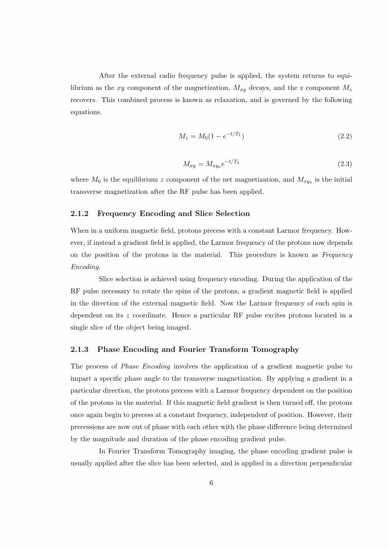
After the external radio frequency pulse is applied, the system returns to equi-

librium as the xy component of the magnetization, Mxy decays, and the z component Mz

recovers. This combined process is known as relaxation, and is governed by the following

equations.

Mz = M0(1 − e−t/T1) (2.2)

Mxy = Mxyoe−t/T2 (2.3)

where M0 is the equilibrium z component of the net magnetization, and Mxyo is the initial

transverse magnetization after the RF pulse has been applied.

2.1.2 Frequency Encoding and Slice Selection

When in a uniform magnetic field, protons precess with a constant Larmor frequency. How-

ever, if instead a gradient field is applied, the Larmor frequency of the protons now depends

on the position of the protons in the material. This procedure is known as Frequency

Encoding.

Slice selection is achieved using frequency encoding. During the application of the

RF pulse necessary to rotate the spins of the protons, a gradient magnetic field is applied

in the direction of the external magnetic field. Now the Larmor frequency of each spin is

dependent on its z coordinate. Hence a particular RF pulse excites protons located in a

single slice of the object being imaged.

2.1.3 Phase Encoding and Fourier Transform Tomography

The process of Phase Encoding involves the application of a gradient magnetic pulse to

impart a specific phase angle to the transverse magnetization. By applying a gradient in a

particular direction, the protons precess with a Larmor frequency dependent on the position

of the protons in the material. If this magnetic field gradient is then turned off, the protons

once again begin to precess at a constant frequency, independent of position. However, their

precessions are now out of phase with each other with the phase difference being determined

by the magnitude and duration of the phase encoding gradient pulse.

In Fourier Transform Tomography imaging, the phase encoding gradient pulse is

usually applied after the slice has been selected, and is applied in a direction perpendicular

6

to the slice selection gradient. Once the phase encoding gradient is removed, the protons in

the slice being imaged precess at a constant frequency, but are out of phase. Subsequently, a

frequency encoding pulse is applied in the direction perpendicular to both the slice selection

and phase encoding gradients and the resulting free induction decay (FID) is measured. The

process from the application of the phase encoding pulse is repeated with phase encoding

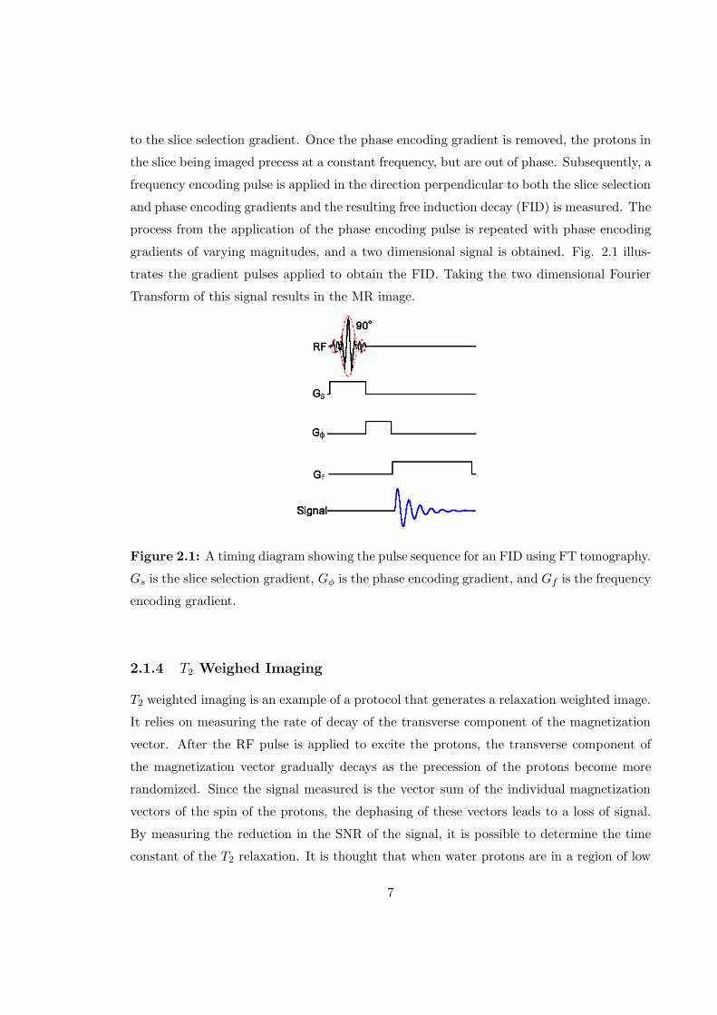
gradients of varying magnitudes, and a two dimensional signal is obtained. Fig. 2.1 illus-

trates the gradient pulses applied to obtain the FID. Taking the two dimensional Fourier

Transform of this signal results in the MR image.

Figure 2.1: A timing diagram showing the pulse sequence for an FID using FT tomography.

Gs is the slice selection gradient, Gφ is the phase encoding gradient, and Gf is the frequency

encoding gradient.

2.1.4 T2 Weighed Imaging

T2 weighted imaging is an example of a protocol that generates a relaxation weighted image.

It relies on measuring the rate of decay of the transverse component of the magnetization

vector. After the RF pulse is applied to excite the protons, the transverse component of

the magnetization vector gradually decays as the precession of the protons become more

randomized. Since the signal measured is the vector sum of the individual magnetization

vectors of the spin of the protons, the dephasing of these vectors leads to a loss of signal.

By measuring the reduction in the SNR of the signal, it is possible to determine the time

constant of the T2 relaxation. It is thought that when water protons are in a region of low

7

viscousity, the T2 relaxation time is slower. The more molecular interractions the faster the

decay.

In a standard MR image, the quantity being measured is the proton density of the

body. In a T2 weighted image, this quantity is weighted by the T2 relaxation properties of

the different regions in the body. The adantage of a T2 weighted image is that the proton

density conveys little information about the type of tissue, and has low contrast if the water

molecules are relatively evenly distributed. The T2 weighted image adds contrast based on

the tissue types of the body being imaged. Such an image is obtained by introducing a

time period between the excitaiton phase and the acquisition phase. This period is called

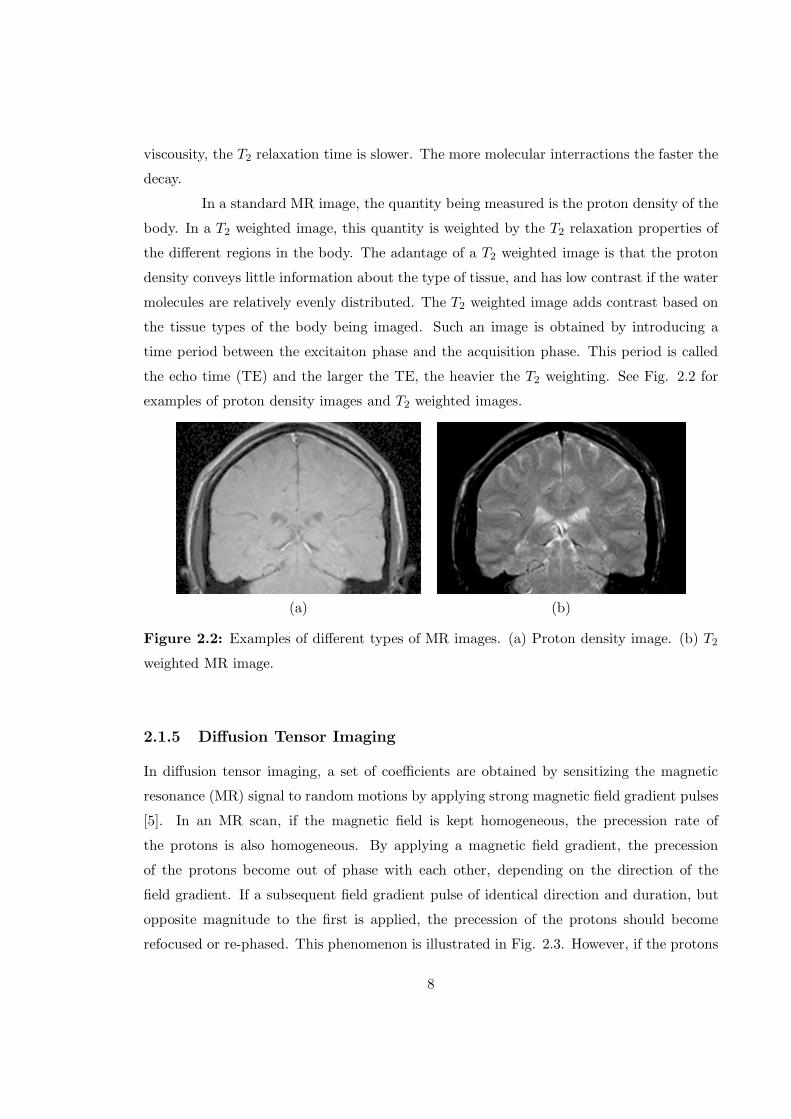
the echo time (TE) and the larger the TE, the heavier the T2 weighting. See Fig. 2.2 for

examples of proton density images and T2 weighted images.

(a) (b)

Figure 2.2: Examples of different types of MR images. (a) Proton density image. (b) T2

weighted MR image.

2.1.5 Diffusion Tensor Imaging

In diffusion tensor imaging, a set of coefficients are obtained by sensitizing the magnetic

resonance (MR) signal to random motions by applying strong magnetic field gradient pulses

[5]. In an MR scan, if the magnetic field is kept homogeneous, the precession rate of

the protons is also homogeneous. By applying a magnetic field gradient, the precession

of the protons become out of phase with each other, depending on the direction of the

field gradient. If a subsequent field gradient pulse of identical direction and duration, but

opposite magnitude to the first is applied, the precession of the protons should become

refocused or re-phased. This phenomenon is illustrated in Fig. 2.3. However, if the protons

8

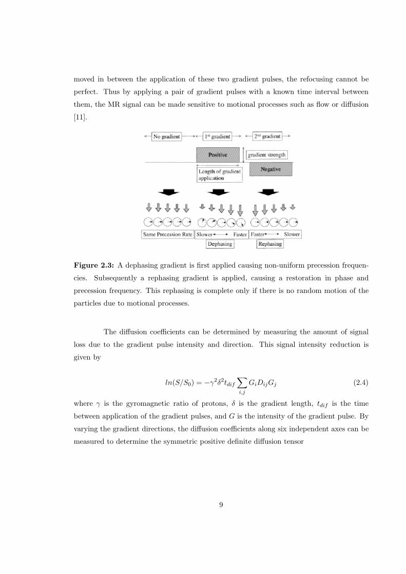
moved in between the application of these two gradient pulses, the refocusing cannot be

perfect. Thus by applying a pair of gradient pulses with a known time interval between

them, the MR signal can be made sensitive to motional processes such as flow or diffusion

[11].

Figure 2.3: A dephasing gradient is first applied causing non-uniform precession frequen-

cies. Subsequently a rephasing gradient is applied, causing a restoration in phase and

precession frequency. This rephasing is complete only if there is no random motion of the

particles due to motional processes.

The diffusion coefficients can be determined by measuring the amount of signal

loss due to the gradient pulse intensity and direction. This signal intensity reduction is

given by

ln(S/S0) = −γ2δ2tdif

∑

i,j

GiDijGj (2.4)

where γ is the gyromagnetic ratio of protons, δ is the gradient length, tdif is the time

between application of the gradient pulses, and G is the intensity of the gradient pulse. By

varying the gradient directions, the diffusion coefficients along six independent axes can be

measured to determine the symmetric positive definite diffusion tensor

9

D =

Dxx Dxy Dxz

Dxy Dyy Dyz

Dxz Dyz Dzz

(2.5)

It is generally accepted that the diffusion tensor matrix characterizes the diffusive

properties of water at a given voxel [12, 14] and if Gaussian diffusion is assumed, the

diffusion tensor matrix corresponds to the covariance matrix of the gaussian distribution

of the direction of diffusion [15]. From this tensor we can derive an ellipsoid associated

with each voxel that is defined by the eigenvalues and eigenvectors of the diffusion tensor

matrix [11]. Once we completely define the ellipsoid it is possible to then use fiber tracking

algorithms to trace various fiber paths. There is evidence to suggest that brain water

diffuses parallel to bundles of axons rather than perpendicular to them [7]. Thus traking the

dominant path of the diffusion of water in the brain allows for the reconstruction of neuronal

projections [5]. Evidence suggests that myocardial heart fibers can also be reconstructed

in a similar manner [9]. In this paper, we outline the use of dynamic programming [13] to

optimally track white matter fibers and myocardial heart fibers.

2.2 Dynamic Programming

2.2.1 Basic Problem

Dynamic programming is a very useful tool that reduces the complexity of the search for a

globally optimal solution on a graph. Its application varies from solving routing problems

in computer networking, to use in speech recognition. Dijkstra’s algorithm in networking,

and Viterbi’s algorithm in speech processing are both instances of dynamic programming.

The basic problem that dynamic programming tries to solve is as follows. Consider

a discrete time dynamic system of the form

xk = f (xk−1, uk−1(xk−1), wk−1) (2.6)

where xk is a state variable, uk is a control or decision variable, and wk is random noise,

with a sequentially additive cost function gk (xk, uk(xk), wk) incurred at each time k, such

that the total cost along a sample trajectory is given by

10

gN (xN ) +

N−1∑

k=0

gk (xk, uk(xk), wk) (2.7)

determine the set of controls { u0, u1, · · · , uN−1 } that minimizes the expected cost

E

[

gN (xN ) +

N−1∑

k=0

gk (xk, uk(xk), wk)

]

(2.8)

The dynamic programming concept relies on the principle of optimality. This

means that if π∗ = { µ∗0, µ

∗1, · · · , µ

∗N−1 } is an optimal control law for the basic problem with

k = 0 · · ·N , then the truncated control law { µ∗i , µ

∗i+1, · · · , µ

∗N−1 } is an optimal control law

for the subproblem of minimizing the cost function

E

[

gN (xN ) +

N−1∑

k=i

gk (xk, uk(xk), wk)

]

(2.9)

with k = i · · ·N .

In the following section, the dynamic programming algorithm and its application to

tracking neuronal projections using diffusion tensor data is discussed further. This problem

is a simplification of the basic problem defined above, as the random noise wk is assumed

to have a zero mean. In this case the problem reduces to determining the optimal control

law { u0, u1, · · · , uN−1 } that minimizes the cost (which is equal to the expected cost)

gN (xN ) +

N−1∑

k=i

gk (xk, uk(xk), wk) (2.10)

2.2.2 Tracking Algorithm

Each voxel in the volume has a symmetric 3 × 3 diffusion tensor (D) and corresponding

eigenelements (λi, φi)i=1,2,3 associated with it. These characterize the diffusive properties

of water at the voxel. In particular the eigenvector associated with the largest eigenvalue

corresponds to the direction of fastest diffusion. Tracking algorithms that employ follow

the principal eigenvalue currently exist [12], [7], [6], [5], though they struggle to track fibers

through regions of low anisotropy, and are generally sensitive to noise.

In order to apply dynamic programming to the problem of tracking optimal curved

trajectories through a volume [3], a fundamentally different approach relative to the current

techniques of tracking the primary eigenvector must be taken. Define the center point of

11

each voxel in the volume to be a node and associate a sequentially additive energy function

with arcs linking neighboring nodes. The problem then reduces to computing the minimum

energy path linking start and end nodes.

Let S be the finite state space of size ||S|| = N and define ck(i, j) as the cost of

the transition from i ∈ S to j ∈ S at time k. If the cost is additive over the length of the

path, and we assume that the optimal path between two points passes through no more

than K nodes, then dynamic programming reduces the complexity of the search to order of

KN2. In applying dynamic programming, we define the state space Sk as the the subset of

nodes that can be reached from the initial node in k steps with a finite cost. In addition,

assume that ck(i, j) ≥ 0, and that ck(i, j) = ∞ implies that no transition from node i to

node j exits. Also, note that the optimal path cannot pass through more than N nodes,

so we set K = N . Furthermore, we permit the degenerate move from a node i to itself

with cost ck(i, i) = 0,∀i. This degenerate move allows paths with length less than N to be

considered.

Definition 1 Given the starting node x0, define node xi as xi = x0 +∑i−1

j=0 vj where vj

is a unit vector in R3. Define PN (x0, xN ) to be all N-length paths starting at node x0 and

ending at node xN . A path π(x0, xN ) ∈ PN (x0, xN ) with cost J(π(x0, xN )) is the sequence

of nodes π(x0, xN ) = {x0, x1, . . . , xN}, with cost J(π(x0, xN )) =∑N−1

i=0 ci(xi, xi+1). The

optimal N-length path is given by

π∗(x0, xN ) = arg minπ∈PN (x0,xN )

N−1∑

i=0

ci(xi, xi+1) (2.11)

Theorem 1 The optimal N-length path cost from node s to node t, J(π∗(s, t)) is given by

J(π∗(s, t)) = J0(s, t), where J0 is given by the final step of the following algorithm, with

JN−1(i, t) = cN−1(i, t), and

Jk(i, t) = minj∈S

{ck(i, j) + Jk+1(j, t)},

where k = 0, 1, . . . , N − 2, i ∈ S and J0(i, t) evaluated at i = s.

Proof The proof is to show that Jk(i, t) is the optimal path cost from node i ∈ S to t ∈ S

in (N − k) moves. Then J0(s, t) is the case where k = 0 evaluated at i = s. We prove this

by induction on k. JN−1(i, t) is clearly the optimal path cost in one move, since there can

be at most one path of length 1 between two nodes. Now suppose that Jn(i, t) is the optimal

12

(N − n) length path cost between nodes i and t. The optimal (N − n + 1) path cost from

node i to node t must be given by Jn−1(i, t) = minj∈S

{ck(i, j) + Jn(j, t)}. Hence the theorem

holds for k = N − 1, N − 2, . . . , 0.

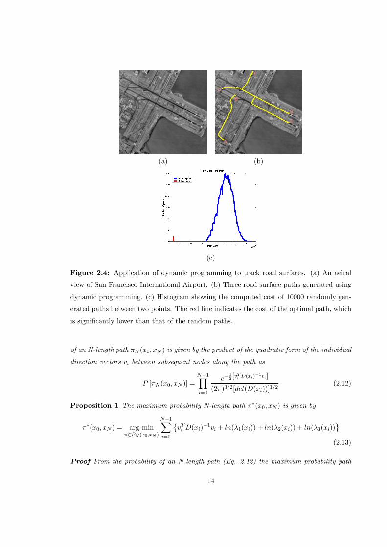
Fig. 2.4 illustrates the application of the dynamic programming algorithm to

the problem of recognizing road surfaces from aerial images [16]. Define each pixel in the

dataset to be a node, and set the cost of a transition from one pixel to another in the

8-neighborhood space to be (I − Iµ)2/σ2, where I is the intensity of the pixel, Iµ is the

mean intensity of a road surface and σ2 is the variance in the intensity of road surfaces in

the data set. Dynamic programming can then be employed to calculate the lowest energy

path as shown in Fig. 2.4(b), where 3 pairs of start and end seed points labelled A-F were

selected. The paths determined by the algorithm travel along low intensity pixels in the

images as these correspond to road surfaces due to the appropriate choice of Iµ and σ. The

histogram in Fig. 2.4(c) shows the drastic difference in path cost between the optimal path

and 10000 other randomly generated paths between points C and D.

2.2.3 Probabilistic Labelling of Paths

Recall from section 2.1.5 that if Gaussian diffusion is assumed in a diffusion tensor MR

image, then the direction of diffusion of water follows a gaussian distribution, with greatest

probability of diffusion in the direction of the primary eigenvector of the diffusion tensor

matrix. Since there is extensive evidence to suggest that the orientation of cortical and

myocardial fibers define the directionality of the diffusion, it is reasonable to assume that

the orientation of fibers in the brain follow the same gaussian distribution as that of the

diffusion of water particles. With this assumption it is possible to show that the problem

of tracking fibers can be reduced to the problem of computing the path between two nodes

in a graph that minimizes a sequentially additive cost function. Define the center of each

voxel in the volume to be a node and the collection of these nodes to represent the state

space S. Also define a voxel j to be in the neighborhood of voxel i if j is immediately

adjacent to i in the 26-connected sense such that there is a direct transition from node xi

to node xj , representing the centers of voxels i and j respectively, if and only if j is in the

neighborhood of i.

Definition 2 Define the probability associated with a transition between connected nodes xi

and xi+1 to have a Gaussian distribution with covariance matrix D(xi). Then the probability

13

(a) (b)

(c)

Figure 2.4: Application of dynamic programming to track road surfaces. (a) An aeiral

view of San Francisco International Airport. (b) Three road surface paths generated using

dynamic programming. (c) Histogram showing the computed cost of 10000 randomly gen-

erated paths between two points. The red line indicates the cost of the optimal path, which

is significantly lower than that of the random paths.

of an N-length path πN (x0, xN ) is given by the product of the quadratic form of the individual

direction vectors vi between subsequent nodes along the path as

P [πN (x0, xN )] =N−1∏

i=0

e−1

2 [vTi D(xi)−1vi]

(2π)3/2[det(D(xi))]1/2(2.12)

Proposition 1 The maximum probability N-length path π∗(x0, xN ) is given by

π∗(x0, xN ) = arg minπ∈PN (x0,xN )

N−1∑

i=0

{

vTi D(xi)

−1vi + ln(λ1(xi)) + ln(λ2(xi)) + ln(λ3(xi))}

(2.13)

Proof From the probability of an N-length path (Eq. 2.12) the maximum probability path

14

is given by

π∗(x0, xN ) = arg maxπ∈PN (x0,xN )

N−1∏

i=0

e−1

2[vT

i D(xi)−1vi]

(2π)3/2[det(D(xi))]1/2(2.14)

By taking the natural log of the equation for the maximum probability path (Eq. 2.14), and

using the fact that det(D(xi)) = λ1(xi)λ2(xi)λ3(xi), we obtain the desired result (Eq. 2.13).

This is a sequentiallly additive cost function and hence it is possible to use dynamic program-

ming to compute the optimal path and its associated cost. The path π∗ = {x0, x1, . . . , xN}

that minimizes this function is the optimal path. Note that the cost function used here

is derived under the model that the orientation of fiber bundles at a given voxel follows a

gaussian distribution with covariance matrix given by the diffusion tensor associated with

that voxel. It is possible to reduce the fiber tracking problem to an optimization problem

as long as the probability distribution can give rise to an additive cost function. In this way

the algorithm can be utilized with a more detailed distribution on the orientation of fibers.

For the purpose of this thesis the gaussian model will be assumed.

As defined in Theorem 1, it is possible to compute the optimal path by searching

over the entire state space S at step k. However, it is possible to apply dynamic program-

ming to reduce the complexity by examining restricted state spaces Sk ⊂ S, and iteratively

computing the optimal N − k length paths, for k = N − 1, N − 2, . . . , 0.

Proposition 2 For any node x ∈ Sk, denote Px as the set of nodes {n} such that a direct

transition from x to n exists. Define the cost ck(xi, xj) = vTi D−1(xi)vi + ln(λ1(xi)) +

ln(λ2(xi)) + ln(λ3(xi)) for xj ∈ Pxi, and ck(xi, xj) = ∞ for xj /∈ Pxi

. The optimal N -

length cost J0(s) from s to t is given by the final step of the following algorithm evaluated

at i = s.

Algorithm 1 Initialize: Jk(i) = ∞ i 6= t, Jk(t) = 0 for all k; SN = {t};

For every k = N − 1 to 0,

Sk = {i|i ∈ Pj , j ∈ Sk+1}; set ck(i, j), i ∈ Sk and j ∈ Sk+1.

Jk(i) = minj∈{Sk+1∩Pi}

{ck(i, j) + Jk+1(j)}, i ∈ Sk

end

Proof The proof is by induction on k. The inductive hypothesis is that Jk(i) is the minimum

cost from node i to node t in (N − k) steps, for all i ∈ Sk. For the initial case k = N this

15

hypothesis is clearly true. Assume it is true for some k = n, and now consider k = n − 1.

Suppose for the sake of contradiction, an optimal path π∗ of length (N − n + 1) from node

i ∈ Sk+1 to node t with cost J∗ < Jn−1(i) exists. Since the path is optimal, then the subpath

of length (N-n) starting from node j ∈ P (i) where j is the second node along the path π∗,

and ending in node t must also be optimal. From the inductive hypothesis, its cost must be

Jn(j), and since j ∈ P (i), we get that J∗ ≥ Jn−1(i), which is a contradiction. Hence the

induction is complete.

Note that the optimal path πk(i) associated with Jk(i) is given recursively by

πN (i) = {t}

πk(i) = πk+1(i) ∪ {j}, where j minimizes Jk

2.2.4 Comparison of DP with other Search Algorithms

In determining the utility of an algorithm it is important to compare the complexity of the

algorithm with other algorithms that can be implemented to solve the problem. Complexity

is characterized by both the runtime of the algorithm on increasingly larger data sets, as

well as the space requirements of the algorithm. Other criteria to judge the utility of a

search algorithm are whether the solution found is guaranteed to be optimal, and whether

the search is complete.

The search problem to be solved in tracking neuronal projections using diffu-

sion tensor imaging involves finding the optimal path between start and end points over

a deterministic search tree. There are numerous strategies that can be employed to solve

this problem. These include a Breadth-First search, a Uniform-Cost search, a Depth-First

search, an Iterative Deepening search, and a Bidirectional search. For a rigorous treat-

ment of each of these strategies, see [17]. Table 2.1 compares these search strategies along

with the dynamic programming algorithm in terms of the criteria of time complexity, space

complexity, optimality of solution, and completeness of the search.

16

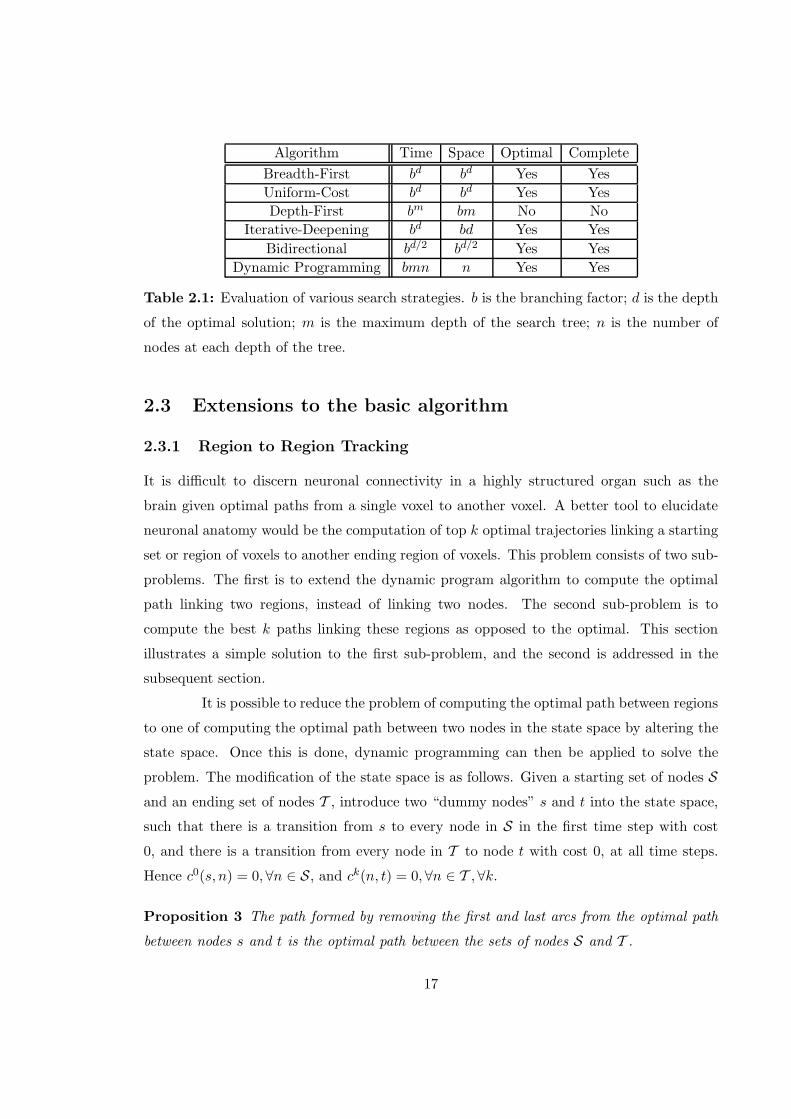
Algorithm Time Space Optimal Complete

Breadth-First bd bd Yes Yes

Uniform-Cost bd bd Yes Yes

Depth-First bm bm No No

Iterative-Deepening bd bd Yes Yes

Bidirectional bd/2 bd/2 Yes Yes

Dynamic Programming bmn n Yes Yes

Table 2.1: Evaluation of various search strategies. b is the branching factor; d is the depth

of the optimal solution; m is the maximum depth of the search tree; n is the number of

nodes at each depth of the tree.

2.3 Extensions to the basic algorithm

2.3.1 Region to Region Tracking

It is difficult to discern neuronal connectivity in a highly structured organ such as the

brain given optimal paths from a single voxel to another voxel. A better tool to elucidate

neuronal anatomy would be the computation of top k optimal trajectories linking a starting

set or region of voxels to another ending region of voxels. This problem consists of two sub-

problems. The first is to extend the dynamic program algorithm to compute the optimal

path linking two regions, instead of linking two nodes. The second sub-problem is to

compute the best k paths linking these regions as opposed to the optimal. This section

illustrates a simple solution to the first sub-problem, and the second is addressed in the

subsequent section.

It is possible to reduce the problem of computing the optimal path between regions

to one of computing the optimal path between two nodes in the state space by altering the

state space. Once this is done, dynamic programming can then be applied to solve the

problem. The modification of the state space is as follows. Given a starting set of nodes S

and an ending set of nodes T , introduce two “dummy nodes” s and t into the state space,

such that there is a transition from s to every node in S in the first time step with cost

0, and there is a transition from every node in T to node t with cost 0, at all time steps.

Hence c0(s, n) = 0,∀n ∈ S, and ck(n, t) = 0,∀n ∈ T ,∀k.

Proposition 3 The path formed by removing the first and last arcs from the optimal path

between nodes s and t is the optimal path between the sets of nodes S and T .

17

Proof Let π∗ be the optimal path between dummy nodes s and t, and let π∗0 be the optimal

path between the sets of nodes S and T . Suppose for the sake of contradiction that π∗0 is

not the path formed by removing the first and last arcs of π∗. Consider the path formed

by prepending the arc between s and the starting node of π∗0 and appending the arc between

the ending node of π∗0 and t. The cost of this path is less than π∗, since π∗

0 is the best path

between the sets S and T , and the costs of the transitions from s to any node in S and

from any node in T to t are 0. However this is a contradiction since π∗ is the optimal path

between s an t, and hence the proposition is true.

From Proposition 3 it is clear that the introduction of the “dummy nodes” into the state

space, does infact lead to the computation of the optimal path between a starting set of

nodes and an ending set of nodes.

2.3.2 Shortest K-Paths Problem

Apart from computing the optimal path from a starting set of nodes to an ending set of

nodes, the determination of the best k paths (as opposed to a single path) can also provide

useful insight into the connectivity of the brain, especially regarding fiber bundles. This

section presents another extension to the dynamic programming algorithm to compute the

optimal k paths between two sets of nodes, described in [18] and [19].

The first step in this algorithm is to determine the shortest path from every other

node in the network to the terminal node, which can be accomplished using algorithm 1.

Note that it is possible to use the same ideas developed in the previous section to track

the best k paths from a start region to a terminal region. Given the optimal path π∗ =

{s = x−1, x0, · · · , xN−1, xN = t} connecting the start and end nodes s and t respectively, it

is possible to compute the best alternative path from s to t. Note that nodes x−1 and xN

are infact “dummy nodes”. To initialize the algorithm, insert a new node x′N into the state

space with c(x′N , xN ) = ∞.

Definition 3 Let Px represent the neighborhood of node x. For any node xi, i ≤ N − 1

along the optimal path π∗, define a new node x′i such that Px′

i= Pxi

+ {x′i+1}−{xi+1}, and

insert this node into the state space S. The cost of the transitions c(x′i, j) = c(xi, j), forj ∈

Pxi∩ Px′

iand c(x′

i, x′i+1) = c(xi, xi+1).

18

The optimal cost J(x′i, xN ) from the newly inserted node x′

i to the terminal node xN is

given by

J(x′i, xN ) = min

j∈Px′i

{c(x′i, j) + J(j, xN )}, (2.15)

and the optimal path is simply the path that results in this minimum cost.

Proposition 4 The optimal cost from node x′i to node xN is the best alternative path cost

from node xi to node xN , i ≤ N − 1.

Proof The proof is by induction on i. Consider the case where i = N − 1. The best

alternative path cost from xN−1 to xN is obtained by searching over all node j ∈ PxN−1−

{xN} and minimizing the quantity c(xN−1, j) + J(j, xN ). However, since Px′

N−1= PxN−1

−

{xN}, the proposition holds for this case. Suppose the proposition is true for i = k, consider

when i = k− 1. The best alternative path cost from xk−1 to xN must either pass through xk

or not pass through xk. If J2(xk, xN ) is the best alternative path from xk to xN , then the

best alternative path cost from xk−1 to xN is given by

min

(

minj∈Pxk−1

−{xk}(c(xk−1, j) + J(j, xN )), c(xk−1, xk) + J2(xk, xN )

)

. (2.16)

Now from the inductive hypothesis, J2(xk, xN ) = J(x′k, xN ), and Px′

k−1= Pxk−1

+ {x′k} −

{xk}, so the induction is complete. As a result the proposition holds.

From Proposition 4, it is possible to compute the best alternative to the optimal path from a

starting set of nodes to an ending set of nodes in the volume by choosing i = −1. Note that

the best alternative to the optimal path is represented by the optimal path from the start

node x−1 to a derivative of the terminal node x′N . Now in order to compute the subsequent

best alternative path it is necessary to repeat the process to find the best alternative path to

the optimal path between x−1 and x′N . By iteratively repeating this process, it is possible

to compute the best k paths connecting start and terminal nodes x−1 and xN , for any

arbitrary k. As illustrated in [19], it is possible to further optimize this algorithm so that

it requires less space. This algorithm is presented below.

Algorithm 2 Define x̄h to be the primed node xh with no primes, x̂h+1 to be the node

immediately subsequent to xh along the path p, and x(k)′h to be the node xh with k primes.

19

Determine the optimal path from every node in S to xN , and let the optimal path from x−1

to xN be p1.

Initialize p = p1, k = 1 and add node x′N to S

While an alternative to p exists and k ≤ K

Set xi = the first node before xN along p

For every xj ∈ {xi, · · · , x(k−1)′−1 }

add node x′j to S

update Px̄j= Px̄j

− {x̂j+1} + {x̂′j+1}

set J(x′j , xN ) = min

n∈Px̄j

{J(n, xN ) + c(x̄j , n)}

end

set p = the optimal path from x(k)′−1 to xN ; k = k + 1

end

2.4 Comparison with Current Algorithms

There are several approaches to extract fiber paths from diffusion tensor MR data,

but the majority of them rely on tracking the direction of the principal eigenvector [7, 6,

12]. Within the framework of the Gaussian distribution on the orientation of fibers such

approaches are equivalent to performing a gradient descent search, iteratively following the

local maximum probability at each voxel until some termination condition is met. While

such an approach will be computationally efficient, the resulting fiber path reconstruction

may not necessarily reflect the optimal path linking two regions as such an approach will

be quite sensitive to noise.

Fig. 2.5 (a) shows a 2D illustration of tracking fiber paths using an approach

relying on locally following the principal direction through a pixel which contain noise,

circled in red on the figure. The tracking veers away in the direction of the noise causing

it to terminate in the adjacent pixel of low anisotropy and as a result the remainder of the

path was not detected. Fig. 2.5 (b) illustrates the path reconstructed from the statistical

tracking using dynamic programming approach with the start and end point known. As

can be seen in the depiction, the cost associated with going against the principal direction

at the corrupted pixel is recovered by continuing along the path. The noise contained in

the corrupted pixel is averaged over the entire path allowing the algorithm to capture the

remaining portion of the path. Since noise and other artifacts that cause the principal

20

eigenvector to deviate from real fiber tracts in the brain are unavoidable, some method to

compensate for this problem is required. The dynamic programming approach provides a

simple method of tracking paths with a reduced sensitivity to noise in the data. There

are approaches to regularize the diffusion tensor data [20] prior to employing a principal

eigenvector tracking approach, but such approaches suffer from the fact that if all the data

isn’t accurately regularized, then the tracking may still be affected.

Another scenario in which algorithms which track the primary eigenvector may

not perform optimally is when individual fibers tracts branch into multiple tracts. Fig. 2.5

(c) illustrates the path reconstructed by tracking the primary eigenvector along a path that

branches into two separate paths. The reconstructed path does not capture the branching.

Fig. 2.5 (d) presents the paths reconstructed using the dynamic programming approach

with the start and end nodes known. The branching effect of the paths is captured since

all paths linking start and end nodes are considered. Progress has been made on this issue

and algorithms to handle branching have been proposed. A notable example of such is the

fast marching tractography technique [21, 22], which is based on an adaptive region growing

approach that propogates a fiber volume from a seed point at varying speeds in different

directions. While this approach solves the problem of tracking fiber paths that branch,

it has a tendency to include a number of false positives in its reconstructions, requiring

additional methods to prune the reconstructed pathways.

Fig. 2.6 (a) and (b) depicts another case in which the dynamic programming

approach and algorithms that track the primary eigenvector produce different results. In

this scenario, there is a central path with high anisotropy with adjacent regions of lower

anisotropy running on either side. Whether or not there are three paths running side by side

is somewhat ambiguous given the data as it is unclear whether the anisotropy in the regions

adjacent to the central path is due to the presence of fiber paths or some partial voluming

effect. It is certain however, that both algorithms will produce distinct results as shown in

(a) and (b). It is possible to extend the base dynamic programming algorithm described in

this paper to incorporate prior knowledge of the curvature and torsion of fiber pathways to

reconstruct more realistic fiber pathways. Fig. 2.6 (c) illustrates how curvature information

can be included in the cost function to change the manner in which paths are reconstructed.

In this case, the curvature of the paths reconstructed by following the primary eigenvector

were used as the prior information. The method of incorporating a priori information into

the dynamic programming cost function is discussed further in chapter 4.

21

There are other proposed statistical approaches to tractography, based on com-

puting a path integral over a detailed orientation distribution function [23] that is solved

using a simulated annealing technique [24]. This approach, which introduces an orienta-

tion distribution model that incorporates a stiffness parameter, has been used to elucidate

connectivity strength between points on the cortex and bears some resemblance to the

method presented here. It should be noted that though the dynamic programming method

is demonstrated to operate on a discretized Gaussian diffusion distribution that incorpo-

rates a priori curvature and torsion properties of fibers, the approach can be adapted to

efficiently compute optimal solutions over any orientation distribution that is approximated

through discretization. The dynamic programming approach guarantees that the computed

solution is optimal in the sense that it maximizes the probability of the path, and with the

improvements we propose it is possible to compute the set of maximum probability paths

linking two regions.

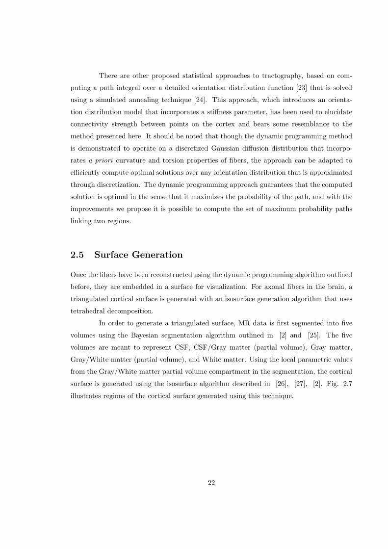
2.5 Surface Generation

Once the fibers have been reconstructed using the dynamic programming algorithm outlined

before, they are embedded in a surface for visualization. For axonal fibers in the brain, a

triangulated cortical surface is generated with an isosurface generation algorithm that uses

tetrahedral decomposition.

In order to generate a triangulated surface, MR data is first segmented into five

volumes using the Bayesian segmentation algorithm outlined in [2] and [25]. The five

volumes are meant to represent CSF, CSF/Gray matter (partial volume), Gray matter,

Gray/White matter (partial volume), and White matter. Using the local parametric values

from the Gray/White matter partial volume compartment in the segmentation, the cortical

surface is generated using the isosurface algorithm described in [26], [27], [2]. Fig. 2.7

illustrates regions of the cortical surface generated using this technique.

22

(a) (b)

(c) (d)

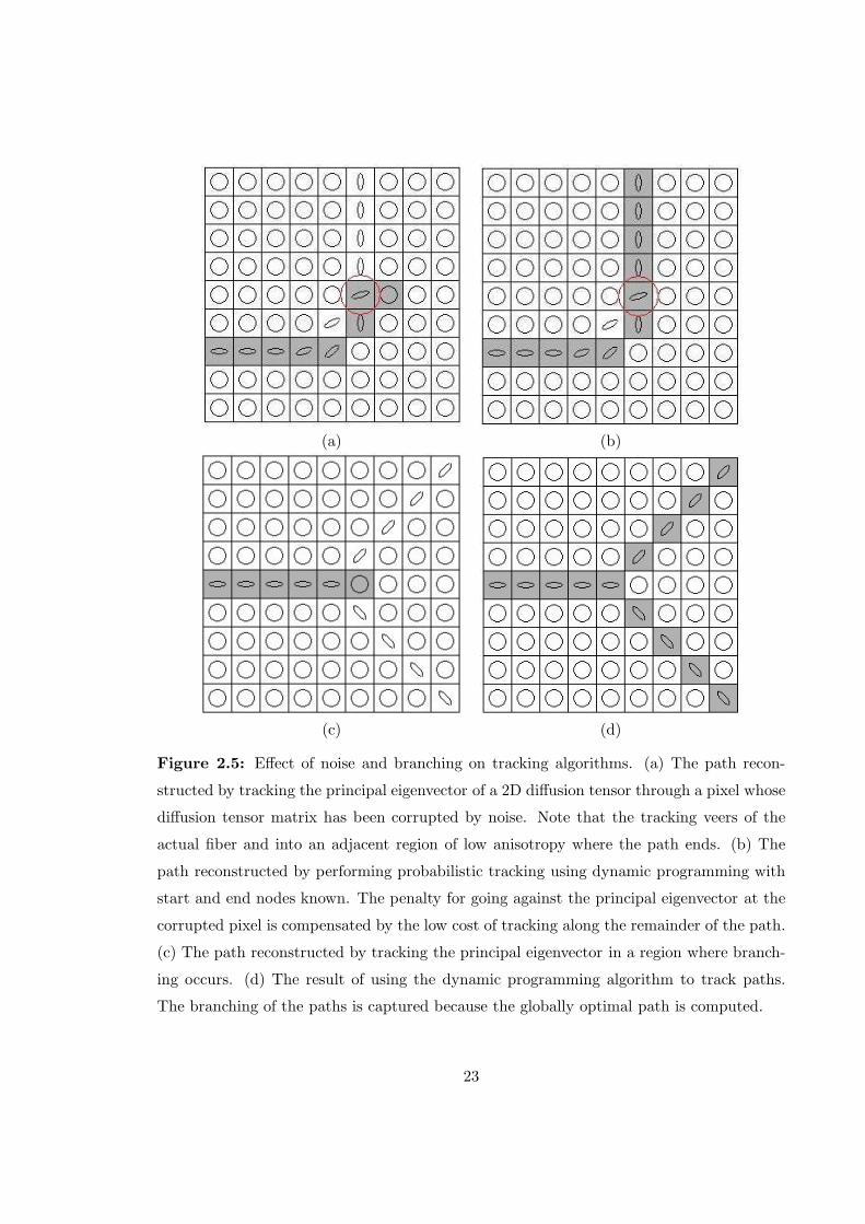
Figure 2.5: Effect of noise and branching on tracking algorithms. (a) The path recon-

structed by tracking the principal eigenvector of a 2D diffusion tensor through a pixel whose

diffusion tensor matrix has been corrupted by noise. Note that the tracking veers of the

actual fiber and into an adjacent region of low anisotropy where the path ends. (b) The

path reconstructed by performing probabilistic tracking using dynamic programming with

start and end nodes known. The penalty for going against the principal eigenvector at the

corrupted pixel is compensated by the low cost of tracking along the remainder of the path.

(c) The path reconstructed by tracking the principal eigenvector in a region where branch-

ing occurs. (d) The result of using the dynamic programming algorithm to track paths.

The branching of the paths is captured because the globally optimal path is computed.

23

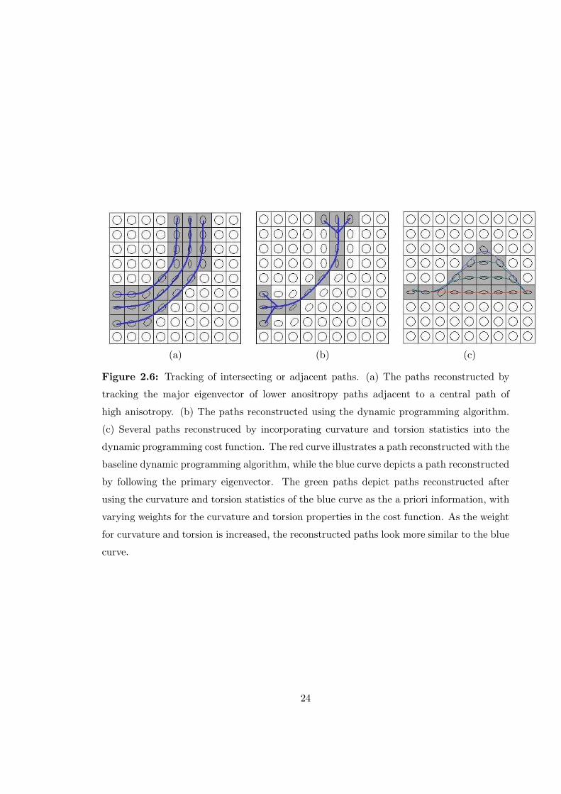
(a) (b) (c)

Figure 2.6: Tracking of intersecting or adjacent paths. (a) The paths reconstructed by

tracking the major eigenvector of lower anositropy paths adjacent to a central path of

high anisotropy. (b) The paths reconstructed using the dynamic programming algorithm.

(c) Several paths reconstruced by incorporating curvature and torsion statistics into the

dynamic programming cost function. The red curve illustrates a path reconstructed with the

baseline dynamic programming algorithm, while the blue curve depicts a path reconstructed

by following the primary eigenvector. The green paths depict paths reconstructed after

using the curvature and torsion statistics of the blue curve as the a priori information, with

varying weights for the curvature and torsion properties in the cost function. As the weight

for curvature and torsion is increased, the reconstructed paths look more similar to the blue

curve.

24

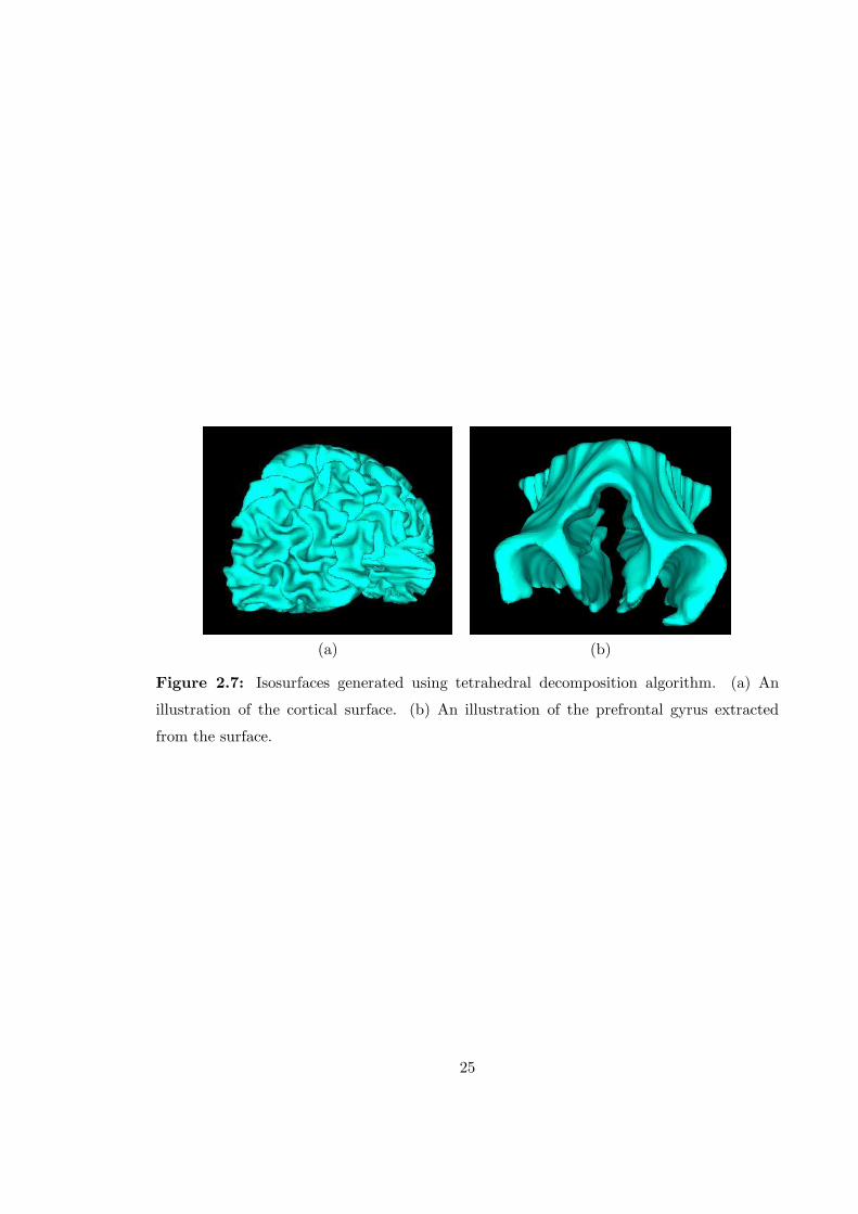
(a) (b)

Figure 2.7: Isosurfaces generated using tetrahedral decomposition algorithm. (a) An

illustration of the cortical surface. (b) An illustration of the prefrontal gyrus extracted

from the surface.

25

Chapter 3

Validation of Algorithm and

Results

3.1 Phantom Data Sets

In order to ensure that the algorithm performs accurately phantom images and diffusion

tensor data are used to test the validity of the algorithm. The results of tracing a path from

a starting point to an end point with various 2 dimensionsal and 3 dimensionsal phantom

data are presented. By examining these results, it can be show that the generated paths

are in fact the minimum energy paths connecting the start and end points.

For this purpose three categories of phantom data sets were generated. Each voxel

has an ellipsoid associated with it. As previously defined the energy associated with moving

from one voxel to an adjacent voxel as being the inverse of the distance between the center

of the ellipsoid and the surface of the ellipsoid in the direction of the neighboring voxel.

For the first category of phantom data sets, all voxels in the image were assigned ellipsoids

that differed only in their size and were identical with respect to their directionality and

anisotropy. Hence the energy associated with moving to an adjacent voxel from a voxel

with a large ellipsoid is much lower than moving to the corresponding adjacent voxel from a

voxel with a small ellipsoid. Hence paths generated using such data sets should move along

regions in the image with large ellipsoids.

For the second category of data sets, each voxel in the image was assigned ellipsoids

that differ only with respect to the direction of the major axis. All ellipsoids are identical in

26

shape and size, but are differently oriented in space depending of the position of the voxel

associated with it. As a result if a path is traced between two voxels, the path should pass

through regoins in the image whose ellipsoids are oriented towards the terminal voxel and

should stay away from regions whose ellipsoids are oriented away from the terminal voxel.

In the third category of phantom data, the principal direction and the volume

of the ellipsoids are held constant, while the anisotropy of the ellipsoids is varied. The

purpose of this phantom data set is to simulate real data. In an actual diffusion tensor MRI

of the human brain, it is believed that regions of high anisotropy in the image correspond

to nerve fibers in the brain. It is know that an ellipsoid with anisotropy in a given direction

corresponds to a low energy associated with moving in that direction. In addition, as the

energy is additive, paths that minimize this energy should move towards regions with high

anisotropy values in the direction of the terminal point.

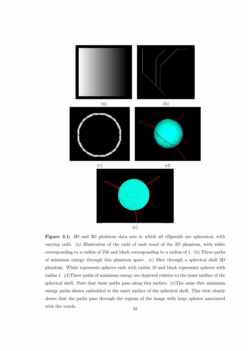
3.1.1 Eigenvalue Variation

This section presents the results of tracing minimum energy paths on 2D and 3D phantom

data sets (Fig. 3.1) in which all voxels possess ellipsoids whose direction and anisotropy are

identical, but whose size varies. We already know that the energy corresponding to moving

from a voxel, in a particular direction depends upon the ellipsoid associated with that voxel.

In particular, this energy is inversely proportional to the distance between the center of the

ellipsoid and the surface of the ellipsoid in the given direction. Hence, all voxels in the image

are assigned ellipsoids that vary only by some constant scale factor, minimum energy paths

should tend to pass through regions with large ellipsoids. This is because larger ellipsoids

correspond to lower costs as the distance between the ellipsoid center and surface in a given

direction is greater than for a smaller, yet otherwise identical ellipsoid.

3.1.2 Eigenvector Variation

Another factor which affects the costs of paths in particular direction is the orientation of the

ellipsoids associated with each voxel. This section presents paths generated from synthetic

diffusion tensor data in which all voxels have ellipsoids that are oriented differently. Apart

from the orientation, all ellipsoids are identical in size and anisotropy. As a result paths

passing through the voxels will have an affinity towards the direction associated with the

highest eigenvalue. So to test the algorithm, set the direction associated with the highest

27

eigenvalue of most of the voxels to be perpendicular to the direction between start and end

points. Also there are a small set of voxels whose directions of the largest eigenvalue are

not perpendicular to the direction between start and end points. In addition, the ellipsoids

are ensured to be highly anisotropic, so that paths passing through the first set of voxels

described above have high costs. Thus, it should be expected to see paths that try to

minimize the passage through these voxels. Fig. 3.2 illustrates the result of the algorithm

through 2D and 3D phantom data sets.

3.1.3 Anisotropy Variation

The degree of anisotropy of the diffusion tensor ellipsoids also have an effect on the cost

function. In diffusion tensor images of the brain and heart, it is thought that directions of

higher anisotropy reflect fiber direction [11], [9]. In this phantom data set, the anisotropy

of the ellipsoids are varied while the eigenvectors remain fixed. If the directions associated

with the largest eigenvalue are oriented towards the end point, paths generated should tend

to pass through the regions of higher anisotropy. 2D and 3D data sets, along with paths

are shown in Fig. 3.3.

3.2 Results

3.2.1 Anisotropy Index

Once the validity of the algorithm was ascertained, fibers were tracked using human brain

and heart diffusion tensor data. A single diffusion tensor MR data set consisting of an MR

image of a human brain and a 3 × 3 tensor value for each voxel in the image was analyzed

and various paths were tracked. Once the eigenvalues and eigenvectors were calculated for

this data set, a cylindrical anisotropy index [12] was calculated for each voxel, defined as

Acyl =λ1 − (λ2 + λ3) /2

λ1 + λ2 + λ1(3.1)

There is significant evidence to suggest that this anisotropy index reflects the degree of fiber

density and myelination of neuronal projections [11]. Hence reconstructed pathways should

pass through regions associated with high anisotropy index. Fig. 3.4 shows this anisotropy

map, highlighting the major regoins in which fibers were tracked.

28

3.2.2 Cortical Neuronal projections

In the human brain the corpus callosum is a thick band of fibers known as the commisural

fibers, located between the cerebral hemispheres [28], [29]. This structure is the primary

connection between the left and right hemispheres of the brain, and as a result any path

traced from one hemisphere to another should traverse along the corpus callosum. We

traced paths through the body of the corpus callosum with starting and ending points in

each hemisphere. The result of one particular tracking experiment is shown in Fig. 3.5

and as expected, the paths connecting regions in different hemispheres passed through the

corpus callosum [5].

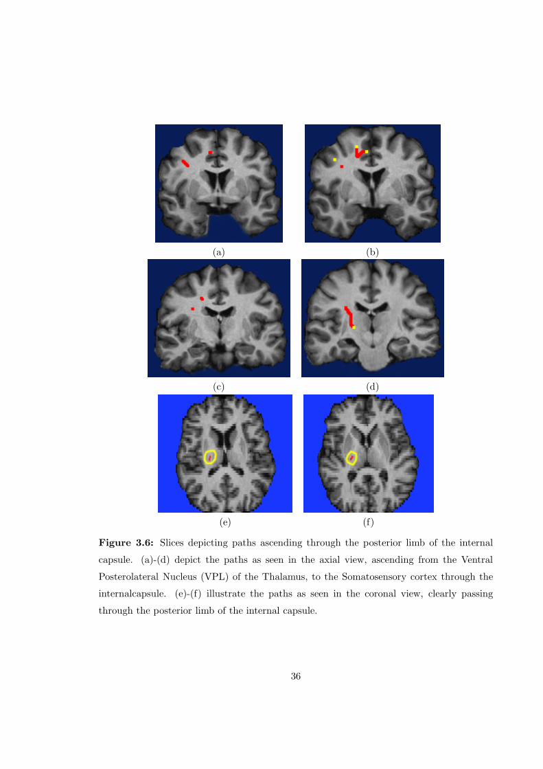
In addition to the corpus callosum, another area of interest are fibers passing

through the internal capsule. The internal capsule is the major structure carrying ascending

and descending projection fibers to and from the cerebral cortex [29], [7], [6]. We attempted

to track fibers from the Ventral Posterolateral Nucleus (VPL) of the Thalamus, to various

regions in the Somatosensory Cortex. It is known that fibers of the sensory pathways that

transmit sensory information to the somatosensory cortex, pass through the posterior limb

of the internal capsule [29]. The paths produced by the dynamic programming algorithm

(Fig. 3.6) are consistent with this anatomy.

A third set of neuronal projection that were reconstruct, are the geniculo-calcarine

visual pathways that connect the lateral geniculate nucleus with the visual cortex, near

the calcarine sulcus. These fibers are responsible for relaying visual information from the

thalymus to the visual cortex. Consistent with known anatomy the fibers generated were

tracked in a posterior direction from the LGN and ran parallel to the occipital horns of the

lateral ventricle [29]. One such fiber can be seen in Fig. 3.7.

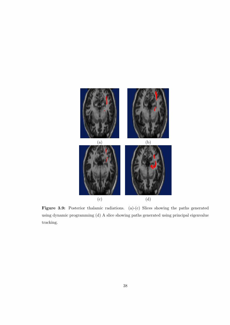
The best K fibers linking regions in the brain were also computed using algorithm

2 and compared to similar fibers generated using principal eigenvalue tracking. The fibers

tracked and compared were the posterior and anterior thalamic radiations, passing horizon-

tally through the internal capsule. The anterior thalamic radiations are thought to connect

the frontal lobe of the brain with the medial and anterior thalamic nuclei, and are known

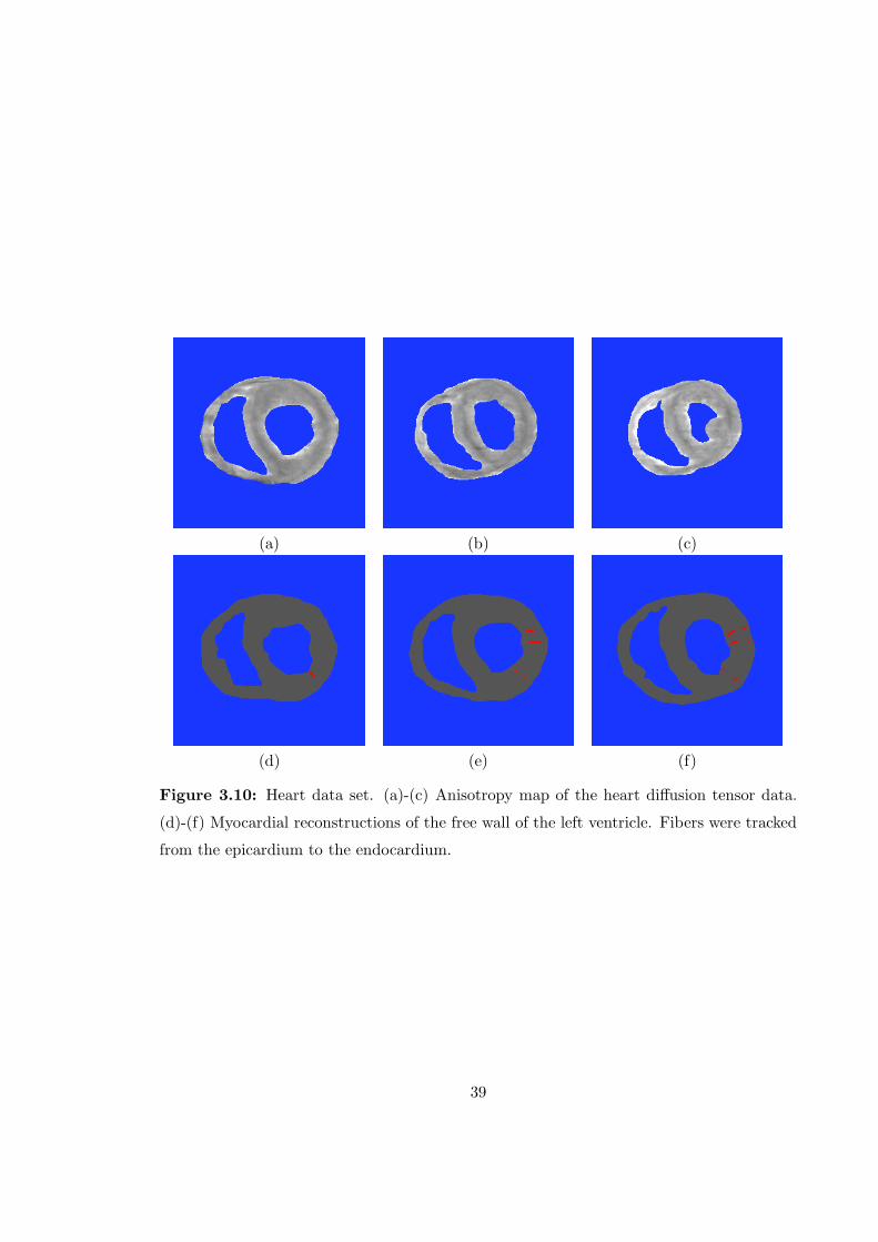
to pass through the anterior limb of the internal capsule [30]. The posterior thalamic radi-

ations connect the posterior and occipital regions of the brain with the caudal portions of

the thalamus. Included in this bundle is the optic radiation which travels from the LGN to

the calcarine cortex [30]. The results of tracking the anterior thalamic radiations using both

29

principal eigenvalue tracking and dynamic programming are shown in Fig. 3.8, and those

for the posterior thalamic radiations are illustrated in Fig. 3.9. The paths created with

principal eigenvalue tracking were based on techniques described in [12]. The paths gener-

ated by each algorithm is generally consistent with known anatomy, though there are some

distinct differences between the two sets of paths. The best K paths generated through

the dynamic programming algorithm linking two regions are more closely bundled than the

paths generated with principal eigenvalue tracking, indicating that the optimal paths are

bundled together and then branch to reach the terminating node. The fiber paths become

less bundled as the value of K is increased. For this experiment a value of K = 2000 was

used, and the fibers produced were more bundled than those produced from the principal

eigenvalue tracking, which number between 200 and 450. Paths generated using principal

eigenvalue tracking are computed by bidirectionally tracking the principal eigenvector of

the diffusion tensor matrix, terminating when the anisotropy falls below a certain thresh-

old. This threshold is usually still in the white matter range, and as a result it becomes

difficult to track paths near gray matter regions. In the case of the dynamic programming

algorithm, the starting and ending regions are specified as constraints for the paths and

thus tracking of paths in regions of low anisotropy is feasable.

3.2.3 Myocardial Fibers

Diffusion tensor MRI data of the heart was also obtained, and myocardial fibers

were reconstructed using the dynamic programming method. It is thought that the walls of

the ventricles are composed of a continuum of fibers that sweep towards the apex of the heart

at the epicardial surface. The fibers also gradually undergo a 180o change in orientation

while passing from the epicardium to the endocardium. Hence the epicardium fibers are

parallel but opposite in direction to the endocardium fibers, while fibers in the midwall

lie perpendicular to these. The anatomic structure of the myocardial fibers is described in

detail in [10], [9], and [8]. Shown in Fig. 3.10 is the anisotropy map for the heart data set.

The epicardial and endocardial walls of both the right and left ventricles exhibit a higher

anisotropy index than the midwall, indicating higher fiber density in these regions. This is

in agreement with [10]. As a result of the geometry of the myocardial fibers, any paths

tracked from the epicardium of the heard towards the endocardium would be expected to

stay in the horizontal or image plane. The result of tracking such fiber paths on the free

30

wall of the left ventricle is shown in Fig. 3.10. As expected, the paths of the deviate very

little from the image plane.

31

(a) (b)

(c) (d)

(e)

Figure 3.1: 2D and 3D phabtom data sets in which all ellipsoids are sphereical, with

varying radii. (a) Illustration of the radii of each voxel of the 2D phantom, with white

corresponding to a radius of 256 and black corresponding to a radius of 1. (b) Three paths

of minimum energy through this phantom space. (c) Slice through a spherical shell 3D

phantom. White represents spheres each with raduis 10 and black represents spheres with

radius 1. (d)Three paths of minimum energy are depicted relative to the inner surface of the

spherical shell. Note that these paths pass along this surface. (e)The same thre minimum

energy paths shown embedded in the outer surface of the spherical shell. This view clearly

shows that the paths pass through the regions of the image with large spheres associated

with the voxels.32

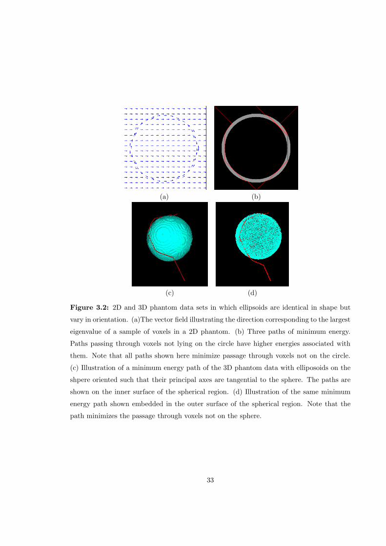
(a) (b)

(c) (d)

Figure 3.2: 2D and 3D phantom data sets in which ellipsoids are identical in shape but

vary in orientation. (a)The vector field illustrating the direction corresponding to the largest

eigenvalue of a sample of voxels in a 2D phantom. (b) Three paths of minimum energy.

Paths passing through voxels not lying on the circle have higher energies associated with

them. Note that all paths shown here minimize passage through voxels not on the circle.

(c) Illustration of a minimum energy path of the 3D phantom data with elliposoids on the

shpere oriented such that their principal axes are tangential to the sphere. The paths are

shown on the inner surface of the spherical region. (d) Illustration of the same minimum

energy path shown embedded in the outer surface of the spherical region. Note that the

path minimizes the passage through voxels not on the sphere.

33

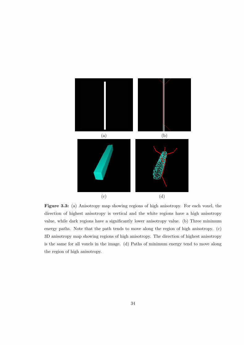
(a) (b)

(c) (d)

Figure 3.3: (a) Anisotropy map showing regions of high anisotropy. For each voxel, the

direction of highest anisotropy is vertical and the white regions have a high anisotropy

value, while dark regions have a significantly lower anisotropy value. (b) Three minimum

energy paths. Note that the path tends to move along the region of high anisotropy. (c)

3D anisotropy map showing regions of high anisotropy. The direction of highest anisotropy

is the same for all voxels in the image. (d) Paths of minimum energy tend to move along

the region of high anisotropy.

34

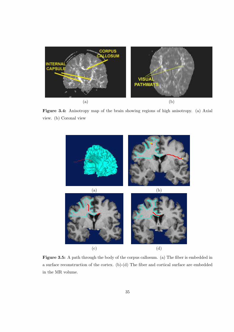
(a) (b)

Figure 3.4: Anisotropy map of the brain showing regions of high anisotropy. (a) Axial

view. (b) Coronal view

(a) (b)

(c) (d)

Figure 3.5: A path through the body of the corpus callosum. (a) The fiber is embedded in

a surface reconstruction of the cortex. (b)-(d) The fiber and cortical surface are embedded

in the MR volume.

35

(a) (b)

(c) (d)

(e) (f)

Figure 3.6: Slices depicting paths ascending through the posterior limb of the internal

capsule. (a)-(d) depict the paths as seen in the axial view, ascending from the Ventral

Posterolateral Nucleus (VPL) of the Thalamus, to the Somatosensory cortex through the

internalcapsule. (e)-(f) illustrate the paths as seen in the coronal view, clearly passing

through the posterior limb of the internal capsule.

36

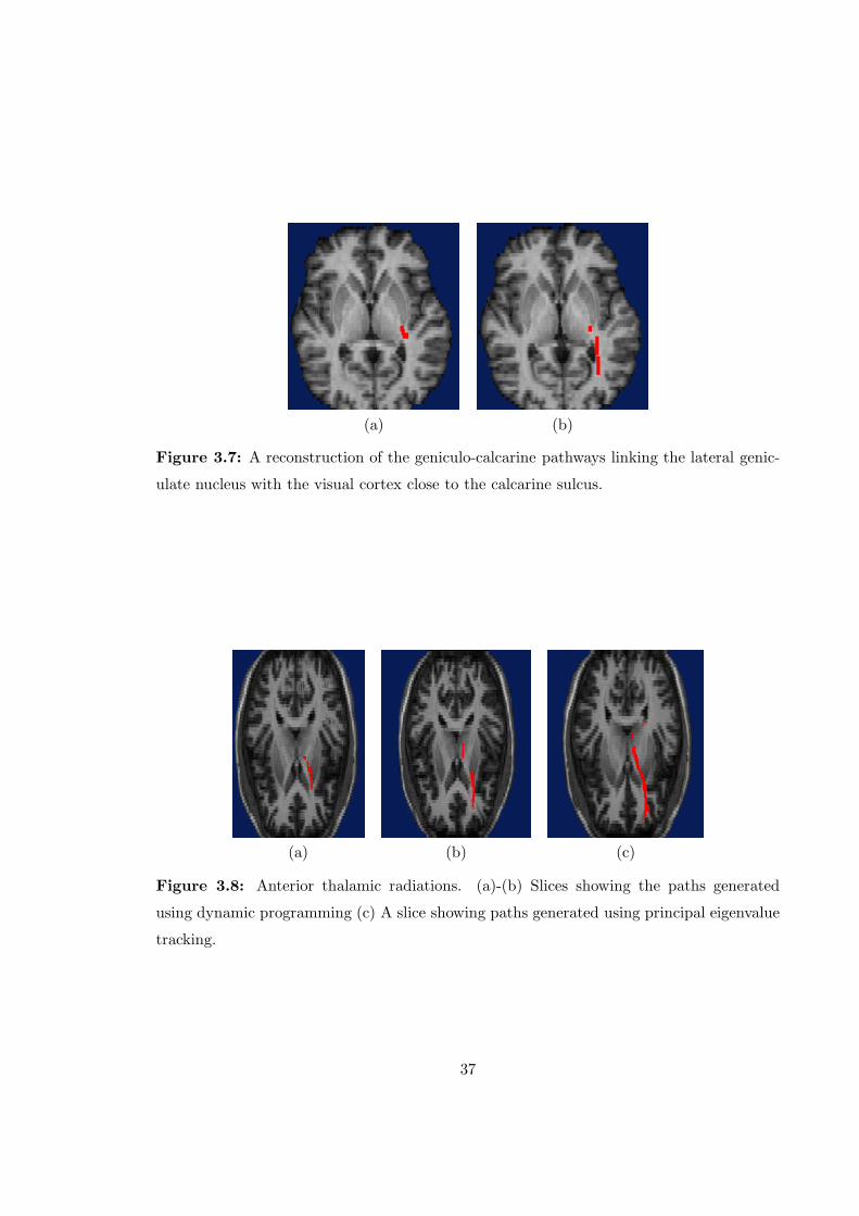
(a) (b)

Figure 3.7: A reconstruction of the geniculo-calcarine pathways linking the lateral genic-

ulate nucleus with the visual cortex close to the calcarine sulcus.

(a) (b) (c)

Figure 3.8: Anterior thalamic radiations. (a)-(b) Slices showing the paths generated

using dynamic programming (c) A slice showing paths generated using principal eigenvalue

tracking.

37

(a) (b)

(c) (d)

Figure 3.9: Posterior thalamic radiations. (a)-(c) Slices showing the paths generated

using dynamic programming (d) A slice showing paths generated using principal eigenvalue

tracking.

38

(a) (b) (c)

(d) (e) (f)

Figure 3.10: Heart data set. (a)-(c) Anisotropy map of the heart diffusion tensor data.

(d)-(f) Myocardial reconstructions of the free wall of the left ventricle. Fibers were tracked

from the epicardium to the endocardium.

39

Chapter 4

Frenet Curve Representation

4.1 Curvature and Torsion

The curves generated by the dynamic programming algorihtm simply minimize an energy

function derived from the diffusion tensor associated with each voxel in the image. These

curves do not utilize any prior knowledge of the geometry of the fibres in the brain. Knowl-

edge of Frenet characteristics such as average curvature and average torsion of fibers can be

incorporated into the cost function of the dynamic programming algorithm [3] to produce

a more realistic representation of the fibers.

The curvature of a unit speed curve α(s) parametrized by arc length can be de-

scribed as a measure of the rate of change of the tangent vector at s. The second derivative

of the curve can be written as, α′′(s) = κ(s)n(s), where n(s) is a unit vector and is called

the normal vector. The unit vectors α′(s) and n(s) define what is called the osculating

plane. The unit normal to this plane b(s) is called the binormal vector at s.

Definition 4 Let α : I → R3 be a curve parametrized by arc length s ∈ I. If the second

derivative is written as α′′(s) = κ(s)n(s), the magnitude κ(s) is called the curvature of α

at s.

Proposition 5 The tangent vector t(s) = α′(s) is perpendicular to the normal vector n(s).

40

Proof By differentiating the equation α′(s) · α′(s) = 1, we get

α′(s) · α′′(s) + α′′(s) · α′(s) = 0

⇒ α′′(s) · α′(s) = 0

⇒ κ(s)n(s) · t(s) = 0.

Hence t(s) ⊥ n(s). �

Proposition 6 The derivative of the binormal vector b′(s) is parallel to the normal vector

n(s).

Proof Recall that b(s) ⊥ b′(s) and that t(s), n(s), and b(s) are mutually orthonormal.

Now, b′(s) ⊥ t(s) since,

b′(s) =d

ds[t(s) × n(s)]

= t′(s) × n(s) + t(s) × n′(s)

= t(s) × n′(s)

Hence b′(s) ‖ n(s) and b′(s) = τ(s)n(s). �

Definition 5 Let α : I → R3 be a curve parametrized by arc length s ∈ I. If the derivative

of the binormal vector is written as b′(s) = τ(s)n(s), the magnitude τ(s) is called the torsion

of α at s.

To implement an algorithm that computes the local curvature and torsion of curves in R3

efficiently, a more mathematically explicit formulation of these parameters is required. To

achieve this, consider the Frenet representation of these curves [3], [31], [4] which gives

rise to what is known as the Frenet formulas.

Proposition 7 The Frenet formulas are defined as

t′(s) = κ(s)n(s) (4.1)

n′(s) = −κ(s)t(s) − τ(s)b(s) (4.2)

b′(s) = τ(s)n(s) (4.3)

41

Proof From Definition 1, α′′(s) = κ(s)n(s) = t′(s). Hence Equation 4.1 holds.

From Definition 2, b′(s) = τ(s)n(s). Hence Equation 4.3 holds.

Since n(s) = b(s) × t(s),

n′(s) = b′(s) × t(s) + b(s) × t′(s)

= −τ(s)b(s) − κ(s)t(s)

Hence Equation 4.2 holds. �

Proposition 8 As per the Frenet representation, if x(·) is a unit speed curve parametrized

by arc length, then the curvature field, κ, is given by

κ(s) =

√

[

d2x1(s)

ds2

]2

+

[

d2x2(s)

ds2

]2

+

[

d2x3(s)

ds2

]2

(4.4)

Proof From Definition 1, κ(s) = ‖α′′(s)‖. Hence Equation 4.4 holds. �

Proposition 9 As per the Frenet representation, if x(·) is a unit speed curve parametrized

by arc length, then the torsion field, τ , is given by

τ(s) =1

κ2(s)

∣

∣

∣

∣

∣

∣

∣

∣

dx1(s)ds

dx2(s)ds

dx3(s)ds

d2x1(s)ds2

d2x2(s)ds2

d2x3(s)ds2

d3x1(s)ds3

d3x2(s)ds3

d3x3(s)ds3

∣

∣

∣

∣

∣

∣

∣

∣

(4.5)

Proof It can easily be seen that the right hand side of Equation 4.5 reduces to t(s) ·(n(s)×

n′(s)). From Equation 4.2 we get that

t(s) · (n(s) × n′(s)) = t(s) · (n(s) × (−τ(s)b(s) − κ(s)t(s)))

= t(s) · (τ(s)t(s) − κ(s)b(s))

= τ(s) �

Equations 4.4 and 4.5 now allow for the efficient computation of local curvature and torsion

of curves in R3, as long as the curve is smooth and differentiable. In the case of fiber

projections, the tracking algorithm outlined in Chapter 2 generates a fiber that is a collection

of discrete points in R3, corresponding to voxels through which the fiber passes. The

computation of curvature and torsion directly depends on the derivatives of the curve.

Thus, in order for the derivatives to be valid it is necessary to fit the set of points defining

the fiber with a smooth and continuous spline curve. The next section details the choice of

the spline fit and its implementation.

42

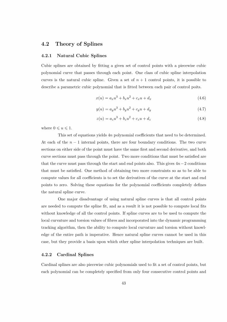
4.2 Theory of Splines

4.2.1 Natural Cubic Splines

Cubic splines are obtained by fitting a given set of control points with a piecewise cubic

polynomial curve that passes through each point. One class of cubic spline interpolation

curves is the natural cubic spline. Given a set of n + 1 control points, it is possible to

describe a parametric cubic polynomial that is fitted between each pair of control poits.

x(u) = axu3 + bxu2 + cxu + dx (4.6)

y(u) = ayu3 + byu

2 + cyu + dy (4.7)

z(u) = azu3 + bzu

2 + czu + dz (4.8)

where 0 6 u 6 1.

This set of equations yields 4n polynomial coefficients that need to be determined.

At each of the n − 1 internal points, there are four boundary conditions. The two curve

sections on either side of the point must have the same first and second derivative, and both

curve sections must pass through the point. Two more conditions that must be satisfied are

that the curve must pass through the start and end points also. This gives 4n−2 conditions

that must be satisfied. One method of obtaining two more constraints so as to be able to

compute values for all coefficients is to set the derivatives of the curve at the start and end

points to zero. Solving these equations for the polynomial coefficients completely defines

the natural spline curve.

One major disadvantage of using natural spline curves is that all control points

are needed to compute the spline fit, and as a result it is not possible to compute local fits

without knowledge of all the control points. If spline curves are to be used to compute the

local curvature and torsion values of fibres and incorporated into the dynamic programming

tracking algorithm, then the ability to compute local curvature and torsion without knowl-

edge of the entire path is imperative. Hence natural spline curves cannot be used in this

case, but they provide a basis upon which other spline interpolation techniques are built.

4.2.2 Cardinal Splines

Cardinal splines are also piecewise cubic polynomials used to fit a set of control points, but

each polynomial can be completely specified from only four consecutive control points and

43

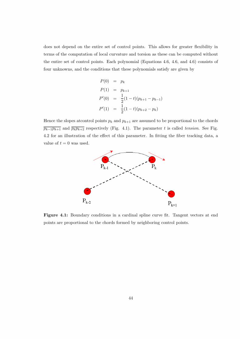
does not depend on the entire set of control points. This allows for greater flexibility in

terms of the computation of local curvature and torsion as these can be computed without

the entire set of control points. Each polynomial (Equations 4.6, 4.6, and 4.6) consists of

four unknowns, and the conditions that these polynomials satisfy are given by

P (0) = pk

P (1) = pk+1

P ′(0) =1

2(1 − t)(pk+1 − pk−1)

P ′(1) =1

2(1 − t)(pk+2 − pk)

Hence the slopes atcontrol points pk and pk+1 are assumed to be proportional to the chords

pk−1pk+1 and pkpk+2 respectively (Fig. 4.1). The parameter t is called tension. See Fig.

4.2 for an illustration of the effect of this parameter. In fitting the fiber tracking data, a

value of t = 0 was used.

Figure 4.1: Boundary conditions in a cardinal spline curve fit. Tangent vectors at end

points are proportional to the chords formed by neighboring control points.

44

Figure 4.2: Illustration of the tension parameter in a cardinal spline curve fit.

4.3 Application to Dynamic Programming

4.3.1 Frenet Analysis of Fibers

Apart from the possibility of containing noise, resolution of diffusion tensor data is not high

enough to isolate individual fibers. Actually, there may be many fibers running through a

given voxel, and the eignevectors of the diffusion tensor matrix can only measure the average

effect of all fibers. As described in earlier sections, incorporation of prior information about

the characteristics of neuronal fibers into the tracking algorithm is desirable as it reduces

the dependence of the algorithm on the diffusion tensor data. Understanding the Frenet

properties of curvature and torsion of fiber curves also serves as a useful tool to compare

fiber paths obtained through computation and through other invasive techniques.

Fig. 4.3 depicts a fiber curve generated through the use of the dynamic program-

ming algorithm. This curve consisted of a set of discrete lattice points, and in order to

compute curvature and torsion, it was necessary to fit the data using cardinal spline inter-

polation. Once this was done, the curvature and torsion at each discrete lattice point on

the fiber was calculated according to Equations 4.4, and 4.5.This analysis is presented in

Fig. 4.3. Using these curvature and torsion plots it is possible to define an L1 norm that

characterizes the distance between a curve, and some other template curve. This distance

is given by

45

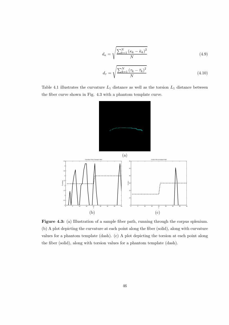
dκ =

√

∑Nk=1 (κk − κ̄k)

2

N(4.9)

dτ =

√

∑Nk=1 (τk − τ̄k)

2

N(4.10)

Table 4.1 illustrates the curvature L1 distance as well as the torsion L1 distance between

the fiber curve shown in Fig. 4.3 with a phantom template curve.

(a)

0 5 10 15 20 25 30 35 400

0.5

1

1.5

2

2.5

3

3.5

4

4.5Curvature Plot of Sample Fiber

k

Cur

vatu

re

0 5 10 15 20 25 30 35 400

10

20

30

40

50

60Torsion Plot of Sample Fiber

k

Tor

sion

(b) (c)

Figure 4.3: (a) Illustration of a sample fiber path, running through the corpus splenium.

(b) A plot depicting the curvature at each point along the fiber (solid), along with curvature

values for a phantom template (dash). (c) A plot depicting the torsion at each point along

the fiber (solid), along with torsion values for a phantom template (dash).

46

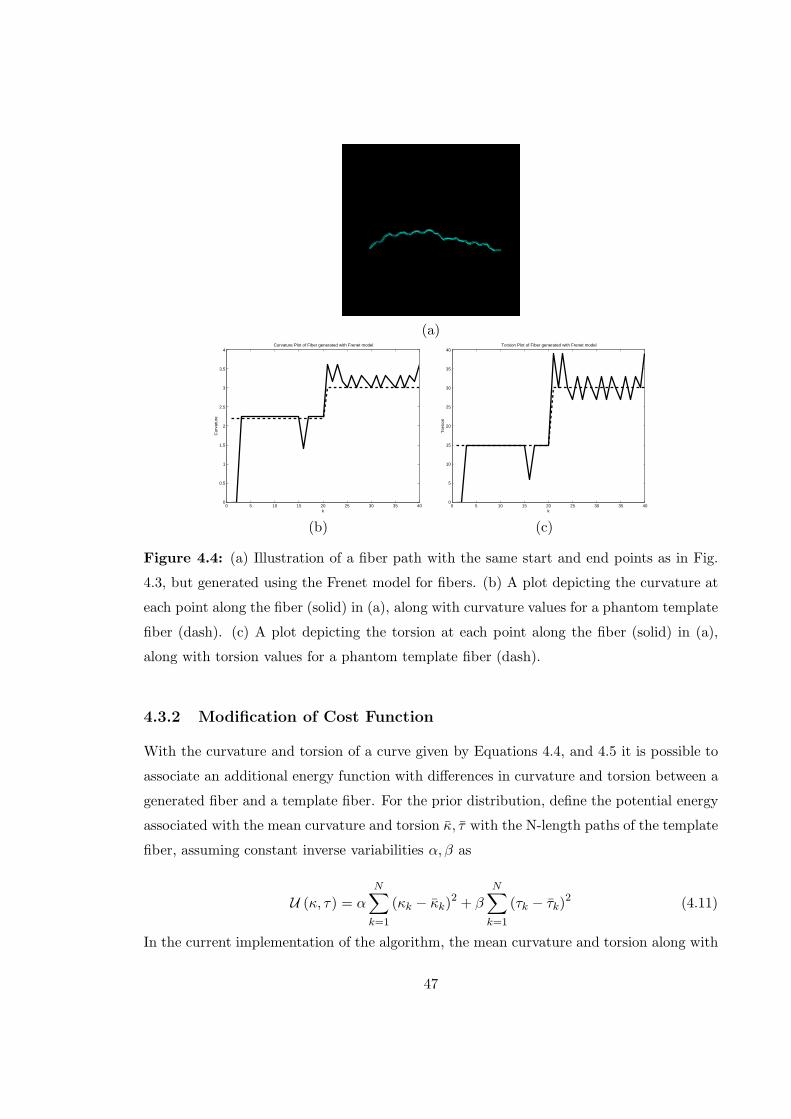
(a)

0 5 10 15 20 25 30 35 400

0.5

1

1.5

2

2.5

3

3.5

4Curvature Plot of Fiber generated with Frenet model

k

Cur

vatu

re

0 5 10 15 20 25 30 35 400

5

10

15

20

25

30

35

40Torsion Plot of Fiber generated with Frenet model

k

Tor

sion

(b) (c)

Figure 4.4: (a) Illustration of a fiber path with the same start and end points as in Fig.

4.3, but generated using the Frenet model for fibers. (b) A plot depicting the curvature at

each point along the fiber (solid) in (a), along with curvature values for a phantom template

fiber (dash). (c) A plot depicting the torsion at each point along the fiber (solid) in (a),

along with torsion values for a phantom template fiber (dash).

4.3.2 Modification of Cost Function

With the curvature and torsion of a curve given by Equations 4.4, and 4.5 it is possible to

associate an additional energy function with differences in curvature and torsion between a

generated fiber and a template fiber. For the prior distribution, define the potential energy

associated with the mean curvature and torsion κ̄, τ̄ with the N-length paths of the template

fiber, assuming constant inverse variabilities α, β as

U (κ, τ) = αN∑

k=1

(κk − κ̄k)2 + β

N∑

k=1

(τk − τ̄k)2 (4.11)

In the current implementation of the algorithm, the mean curvature and torsion along with

47

their variabilities are left as parameters that the user can set, since accurate template fibers

were not available. However, analysis in which phantom values are assigned as template

curvature and torsion is presented so as to provide a framework to understand how esti-

mated mean curvature and torsion values would be used in conjunction with the dynamic

programming algorithm in the event that accurate template data from other (perhaps in-

vasive) imaging sources becomes available.

The empirical estimates of the mean curvature and torsion and their variabilities

would be defined for similarly shaped fibers, according to the formulas

ˆ̄κk =1

M

M∑

m=1

κ(m)k , ˆ̄τ k =

1

M

M∑

m=1

τ(m)k (4.12)

α̂−1 =1

MN

M∑

m=1

N∑

k=1

(κ(m)k − ˆ̄κk)

2, β̂−1 =1

MN

M∑

m=1

N∑

k=1

(τ(m)k − ˆ̄τk)

2 (4.13)

where N is the length of the template fibers, and M is the number of fibers used in the

estimate. In this experiment, the mean curvature and torsion at each point on the fiber is

given by Fig. 4.3, and their variabilities were assigned values of 1.

The potential energy defined in Equation 4.11 was then incorporated into the cost

function of the dynamic programming algorithm in order to accomodate prior information

of the geometric properties of the fibers. The curvatures and torsions of the paths were

calculated by first fitting cardinal splines [32] to the nodes of the fiber paths. The new cost

function Ek(x, y) between two points x ∈ Sk and y ∈ Sk+1 is given by

Ek(x, y) = ck(x, y) + α (κk − κ̄k)2 + β (τk − τ̄k)

2 (4.14)

It should be noted however, that curvature and torsion estimates of an arc connecting two

points on the path depend on other points comprising the path. In this implementation

in which cardinal splines are first fitted to the data to compute the curvature and torsion

values, these values depend on the two previous nodes along the path. Hence the cost

defined in Eq. 4.14 also implicitly depends on these 4 points and for dynamic programming

to generate the optimal solution, the state space of the algorithm has to be modified. In

order for the cost function in Eq. 4.14 to depend only on nodes x ∈ Sk and y ∈ Sk+1, the

definition of a node has to be modified.

48

Definition 6 Denote the center of any voxel in the volume to be a point. Define a node x

to be a set of 3 points that correspond to 3 adjacent voxels in the volume, x = {p, q, r|q ∈

Np, r ∈ Nq}, where Nv is the neighborhood of point v. A transition exists between nodes

xi = {p, q, r} and node xi+1 = {q, r, s} if s ∈ Nr. The cost of this transition is given by

Ek(xi, xi+1) = ck(r, s) + α (κk (q, r, s, t) − κ̄k)2 + β (τk (q, r, s, t) − τ̄k)

2 . (4.15)

With this changes to the state space, computing the optimal path between points s and t

is now reduced to computing the optimal path between node s = {s, s, s} and t = {t, t, t}.

Proposition 10 For any node x = {p, q, r} ∈ Sk, denote Px as the set of nodes {n =

{q, r, s}} such that s ∈ Nr. Define the cost Ek (xi, xj) as in Eq. 4.15 for xj ∈ Pxi, and

Ek (xi, xj) = ∞ for xj /∈ Pxi. The optimal N-length cost J0 (s) from s to t is given by the

final step of the following algorithm evaluated at i =s.

Algorithm 3 Initialize: Jk(i) = ∞ i 6= t, Jk(t) = 0 for all k; SN = {t};

For every k = N − 1 to 0,

Sk = {i|i ∈ Pj , j ∈ Sk+1}; set Ek(i, j), i ∈ Sk and j ∈ Sk+1.

Jk(i) = minj∈{Sk+1∩Pi}

{Ek(i, j) + Jk+1(j)}, i ∈ Sk

end

Proof Proposition 2 holds since the cost function Ek(i, j) is sequentially additive, and

depends only on nodes i ∈ Sk and j ∈ Sk+1.

Implementing the modified dynamic programming algorithm described in Algorithm 3 leads

to a reduction in efficiency as the state space over which the search is performed is increased.

Hence there is a trade off between a priori knowledge regarding mean curvature and mean

torsion, and the optimality of the solution computed. To handle efficiency issues the current

implementation does not use this increased state space algorithm and the optimal path

search is carried out using the dynamic programming algorithm described in Algorithm 1.

As a result the solution computed is an approximate.

Using this energy function which includes information about the prior knowledge

of the Frenet properties of the fibers as the cost function, fiber curves were traced with

the dynamic programming algorithm. Fig. 4.4 depicts the path, and its curvature and

torsion plots along with the template curvature and torsion plots. Due to the quadratic

49

Fiber Curvature L1 Distance Torsion L1 Distance

Dynamic Programming 28.08 6.08

Frenet Model 2.08 1.61

Table 4.1: Curvature and Torsion L1 distances between the fiber generated through the

dynamic programming algorithm without prior Frenet information and template fiber, and

between the fiber generated with the dynamic programming algorithm with prior Frenet

information and the template fiber.

cost associated with inconsistencies in torsion, the newly generated curve has a high degree

of torsion. Also, table 4.1 shows the curvature L1 distance as well as the torsion L1 distance

between the fiber and the phantom template curve.

50

Chapter 5

Conclusion and Future Directions

The major contribution of this thesis was the extension of concepts based in the field of

computational anatomy, particularly dynamic programming and the Frenet representation

of curves, to solve the problem of tracking myocardial and cortical fibers using diffusion

tensor imaging, as described in Chapter 2. The algorithm presented is based on dynamic

programming, and similar to work done in curve extraction from brain surfaces [3], and

boundary [33] and artery tracking [34], [35].

The primary advantage of this method over other current tracking techniques is

that a globally optimal path linking two regions is obtained. The current techniques used

to solve this problem assume that the direction of fastest diffusion of water at each voxel in

the data corresponds to the orientation of fiber paths. As a result such methods will be less

stable to noise. With the dynamic programming approach, as the optimization problem

is globally solved, noise in individual voxels along a path is averaged over the entire path

making the algorithm more robust to random fluctuations in the data. The addition of

Frenet properties to the cost function of the algorithm also permits the reconstruction of

more realistic fibers by accounting for prior knowledge of fiber characteristics of curvature

and torsion.

To summarize, by using a dynamic programming algorithm and diffusion tensor

imaging of human subjects, 3D representations of human cortical and myocardial projections

were reconstructed. In addition to rigorously testing the algorithm on various phantom

data sets, the commisural fibres through the corpus callosum, as well as fibers ascending

through the internal capsule to regions in the somatosensory cortex were traced. Fibers

of the geniculo-calcarine visual pathways, as well as myocardial fibers running from the

51

epicarduim to the endocardium of the free wall of the left ventricle were tracked. The

algorithm was then extended to incorporate prior information of the Frenet characteristics

of curvature and torsion into the cost function of the dynamic programming algorithm.

Key applications of the approaches described in this thesis range from providing a

means to better understanding anatomical structures in the brain and heart, to providing

tools to help in diagnosing disorders of these organs. Specific knowledge of the anatomy

of our brain and heart and understanding the variation across healthy and diseased organs

will contribute tremendously to diagnosis and treatment of several ailments. Greater under-

standing of the connectivity in the brain will also be a powerful tool in functional research

on the brain. To meet these needs, future direction of this work would include the creation

of a database of white matter and myocardial fibers for brains and hearts in different states.

The comparison of density and direction of cortical and myocardial fibers in normal adults

and aging adults, as well as in diseased brains and hearts could yield valuable data on how

the aging process and various diseases such as stroke and tumor growth in the brain, and

arrhythmia, ischemia and ventricular hypertrophy in the heart, affect the fibers. This data

could then have high diagnostic value.

52

Bibliography

[1] U. Grenander and M. I. Miller, “Computational anatomy: An emerging discipline,”

Quarterly of Applied Mathematics, vol. 56, pp. 617–694, 1998.

[2] M. Joshi, J. Cui, K. Doolittle, S. Joshi, D. V. Essen, L. Wang, and M. Miller, “Brain

segmentation and the generation of cortical surfaces,” NeuroImage, vol. 9, pp. 461–476,

1999.

[3] N. Khaneja, U. Grenander, and M. Miller, “Dynamic programming generation of curves

on brain surfaces,” Pattern Analysis and Machine Intelligence, vol. 20, pp. 1260–1264,

1998.

[4] M. Bakircioglu, U. Grenander, N. Khaneja, and M. Miller, “Curve matching on brain

surfaces using frenet distances,” Human Brain Mapping, vol. 6, pp. 329–333, 1998.

[5] T. Conturo, N. Lori, T. Cull, E. Akbudak, A. Snyder, J. Shimony, R. McKinstry,

H. Burton, and M. Raichle, “Tracking neuronal fiber pathways in the living human

brain,” Proceedings of the National Academy of Science USA, vol. 96, pp. 10422–10427,

1999.

[6] S. Mori, W. Kaufmann, G. Pearlson, B. Crain, B. Stieltjes, M. Solaiyappan, and P. van

Zijl, “In vivo visulization of human neuronal pathways by magnetic resonance imaging,”

Annals of Neurology, vol. 47, pp. 412–414, 2000.

[7] S. Mori, B. Crain, V. Chacko, and P. van Zijl, “Three-dimensional tracking of axonal

projections in the brain by magnetic resonance imaging,” Annals of Neurology, vol. 45,

pp. 265–269, 1999.

[8] R. Berne and M. Levy, Cardiovascular Physiology, Seventh Edition. St. Louis, MI:

Mosby-Year Book, Inc., 1997.

53

[9] E. W. Hsu, A. L. Muzikant, S. A. Matulevicius, R. C. Penland, and C. S. Henriquez,

“Magnetic resonance myocardial fiber-orientation mapping with direct histological cor-

relation,” American Journal of Physiology: Heart and Circulatory Physiology, vol. 274,

pp. H1627–H1634, 1998.

[10] D. Scollan, A. Holmes, R. Winslow, and J. Forder, “Histological validation of myocar-

dial microstructure obtained from diffusion tensor magnetic resonance imaging,” Amer-

ican Journal of Physiology: Heart and Circulatory Physiology, vol. 275, pp. H2308–

H2318, 1998.

[11] S. Mori and P. Barker, “Diffusion magnetic resonance imaging: Its principle and ap-

plications,” The Anatomical Record (New Anat.), vol. 257, pp. 102–109, 1999.

[12] R. Xue, P. van Zijl, B. Crain, M. Solaiyappan, and S. Mori, “In vivo three-dimensional

reconstruction of rat brain axonal projections by diffusion tensor imaging,” Magnetic

Resonance in Medicine, vol. 42, pp. 1123–1127, 1999.

[13] D. P. Bertsekas, Dynamic Programming. Englewood Cliffs, NJ: Prentice-Hall, Inc.,

1987.

[14] D. Le Bihan, J.-F. Mangin, C. Poupon, C. Clark, S. Pappata, N. Molko, and

H. Chabriat, “Diffusion tensor imaging: Concepts and applications,” Journal of Mag-

netic Resonance Imaging, vol. 13, pp. 534–546, 2001.

[15] A. L. Alexander, K. Hasan, G. Kindlmann, D. L. Parker, and J. S. Tsurudal, “A

geometric analysis of diffusion tensor measurements of the human brain,” Magnetic

Resonance in Medicine, pp. 283–291, 2000.

[16] M. Fischler, J. Tenenbaum, and H. Wolf, “Detection of roads and linear structures

in low-resolution aerial imagery using a multisource knowledge integration technique,”

Computer Graphics and Image Processing, vol. 15, pp. 210–223, 1981.

[17] S. Russell and P. Norvig, Artificial Intelligence: A Modern Approach (second edition).

Prentice-Hall, Englewood Cliffs, NJ, 2003.

[18] J. A. de Azevedo, J. J. . E. R. S. Madeira, E. Q. V. Martins, and F. M. A. Pires, “A

shortest paths ranking algorithm,” in Proc. AIRO’90, (Genova, Italy), pp. 1001–1011,

Operational Research Society of Italy, 1990.

54

[19] E. Q. V. Martins and J.-L. E. Santos, “A new shortest paths ranking algorithm,”

Investigacao Operacional, vol. 20, pp. 47–62, 2000.

[20] C. Poupon, C. Clark, V. Frouin, J. Regis, I. Bloch, D. Le Bihan, and J.-F. Mangin,

“Regularization of diffusion-based direction maps for the tracking of brain white matter

fasicles,” NeuroImage, vol. 12, pp. 184–195, 2000.

[21] G. Parker, K. Stephan, G. Barker, J. Rowe, D. MacManus, C. Wheeler-Kingshott,

O. Ciccrelli, R. Passingham, R. Spinks, R. lemon, and R. Turner, “Initial demonstra-

tion of in vivo tracing of axonal projections in the macaque brain and comparison

with the human brain using diffusion tensor imaging and fast marching tractography,”

NeuroImage, vol. 15, pp. 797–809, 2002.

[22] G. Parker, C. Wheeler-Kingshott, and G. Barker, “Estimating distributed anatomical

connectivity using fast marching methods and diffusion tensor imaging,” IEEE Trans.

Medical Imaging, vol. 21, pp. 505–512, 2002.

[23] D. Tuch, J. W. Belliveau, and V. Wedeen, “A path integral approach to white matter

tractography,” Proc. Intl. Soc. Mag. Reson. Med., vol. 8, p. 791, 2000.

[24] D. Tuch, M. Wiegell, T. Reese, J. W. Belliveau, and V. Wedeen, “Measuring cortico-

cortical connectivity matrices with diffusion spectrum imaging,” Proc. Intl. Soc. Mag.

Reson. Med., vol. 9, p. 502, 2001.

[25] M. Miller, A. Massie, J. Ratnanather, K. Botteron, and J. Csernansky, “Bayesian

construction of geometrically based cortical thickness metrics,” Neuroimage, vol. 12,

pp. 676–682, 2000.

[26] A. Gueziec and R. Hummel, “Exploiting triangulated surface extraction using tetra-

hedral decomposition,” IEEE Transactions on Visualization and Computer Graphics,

vol. 1, pp. 328–342, dec 1995.

[27] M. Joshi, “Connected brain segmentation and cortical surface generation,” Master’s

thesis, Department of Electrical Engineering, Sever Institute of Technology, Washing-

ton University, St. Louis,MO, August 1998.

[28] H. M. Duvernoy, The Human Brain. New York: Springer-Verlag, 1991.

55

[29] D. Haines, Neuroanatomy: An Atlas of Structures, Sections and Systems. Baltimore,

MD: Urban and Schwarzenberg, 1991.

[30] M. B. Carpenter, Core Text of Neuroanatomy. Baltimore, MD: William and Wilkins,

1991.

[31] N. Khaneja, “Statistics and geometry of cortical features,” Master’s thesis, Department

of Electrical Engineering, Sever Institute of Technology, Washington University, St.

Louis,MO, December 1996.

[32] D. Hearn and M. Baker, Computer Graphics. Englewood Cliffs, NJ: Prentice-Hall, Inc.,

1994.

[33] D. Cooper, H. Elliott, F. Cohen, L. Reiss, and P. Symosek, “Stochastic boundary esti-

mation and object recognition,” Image Modeling, Academic Press, New York, pp. 63–

94, 1981.

[34] R. Petrocelli, J. Elion, and M. Manbeck, “A new method for structure recognition

in unsubtracted digital angiograms,” Proceedings of Computers in Cardiology IEEE

Computer Society, pp. 207–210, October 1992.

[35] R. Petrocelli, K. Manbeck, and J. Elion, “Three dimensional structure recognition in

digital angiograms using gauss-markov methods,” Proceedings of Computers in Cardi-

ology IEEE Computer Society, pp. 329–333, September 1993.

56

Curriculum Vitæ

Rakesh M. Lal was born in San Fernando, Trinidad and Tobago on April 19, 1978. In

1998, he was accepted into the combined Bachelor/Master of Science in Engineering

in Biomedical Engineering at the Johns Hopkins University, Baltimore, Maryland.

He graduated with Bachelor of Science in Engineering degrees in Biomedical Engi-

neering and Computer Science from the Johns Hopkins University in May 2001, and

he is expected to complete his Master of Science in Engineering degree in Biomedical

Engineering by April 2004. His research interests include computational anatomy,

differential geometry, image processing and analysis, and scientific computing.

57