MNRAS 443, 423–431 (2014) doi:10.1093/mnras/stu1159

Probabilistic model for constraining the Galactic potential using tidalstreams

Jason L. Sanders‹

Rudolf Peierls Centre for Theoretical Physics, Keble Road, Oxford OX1 3NP, UK

Accepted 2014 June 9. Received 2014 June 9; in original form 2014 January 29

ABSTRACTWe present a generative probabilistic model for a tidal stream and demonstrate how this modelis used to constrain the Galactic potential. The model takes advantage of the simple structureof a stream in angle and frequency space for the correct potential. We investigate how themethod performs on full 6D mock stream data, and mock data with outliers included. Ascurrently formulated, the technique is computationally costly when applied to data with largeobservational errors, but we describe several modifications that promise to make the techniquecomputationally tractable.

Key words: methods: numerical – Galaxy: kinematics and dynamics – Galaxy: structure –galaxies: kinematics and dynamics.

1 IN T RO D U C T I O N

A key goal in the study of the Milky Way is mapping the dark matterdistribution of the Galaxy. Locally, this is achieved through dynam-ical measurements of the disc components (Kuijken & Gilmore1989; Bovy & Tremaine 2012; Garbari et al. 2012; Zhang et al.2013), whilst tidal streams present a tantalising prospect for con-straining the dark matter distribution on a more global scale. Theselong, filamentary structures are the remnants of satellites tidallydisrupted by the Milky Way. The stars in the stream are now essen-tially orbiting freely in the Galactic potential, but importantly theyform a dynamically coherent structure, such that their properties areclosely linked together. By inspecting the phase-space structure oftidal streams, it should be possible to infer properties of the Galacticpotential, and in particular, the dark matter distribution.

Many methods have been proposed to achieve this. The sim-plest, and therefore most fruitful to-date, are orbit-fitting techniques(Binney 2008; Eyre & Binney 2009a,b; Koposov, Rix & Hogg 2010;Deg & Widrow 2014). Several authors have acknowledged the prob-lems with simply fitting a stream with a single orbit (Eyre & Binney2011; Lux et al. 2013; Sanders & Binney 2013a). Therefore, muchwork has been done on constructing methods for recovering the po-tential without assuming the stream delineates an orbit. One groupof methods seeks the potential which minimizes the spread in theintegrals of motion (Penarrubia, Koposov & Walker 2012). Othersallow for the expected range of orbits present in a stream giventhe progenitor properties (Johnston et al. 1999; Varghese, Ibata &Lewis 2011; Price-Whelan & Johnston 2013).

The dynamics of tidal streams are very simply expressed in angle–action coordinates (Helmi & White 1999; Tremaine 1999; Eyre &

� E-mail: jason.sanders@physics.ox.ac.uk

Binney 2011) denoted as (θ , J) throughout the paper. In Sanders &Binney (2013b), we demonstrated the power of using the frequen-cies and angles of the stream to construct a measure of the goodnessof fit of the potential. The frequencies, �, are the derivatives of theHamiltonian, H, with respect to the actions i.e. � = ∂H/∂ J . Thebest potential was deemed the one in which the angle and frequencydistributions are aligned. This method suffered several drawbacks:we were doing the inference in model space, not the data space; itwas difficult to assess the errors in the obtained potential parame-ters; it was awkward to handle errors in the data, and the methoddid not behave well for large errors.

Data for tidal streams have large errors and are expected to be con-taminated with non-stream members. Streams lie at large distancesfrom the Sun, far out in the halo. As such, the distance uncertain-ties can be significant, and small proper motion errors translate intolarge transverse velocity errors. For many streams we do not havefull 6D data. Additionally, a stream is identified as a filament in theobservable space – often l and b. Stream members are then extractedby cutting appropriately in these coordinates, and cleaning up byusing the additional observables. This process obviously introducesmany outliers to the stream data, which are perhaps just membersof a smoother background halo, whilst also potentially throwing outstars which are members of the stream.

This state of affairs leads us to analyse the data by constructingprobabilistic models that correctly handle large errors, missing dataand contaminants. Such an approach is much more robust thanprevious efforts, and lends itself perfectly to being combined withother independent measurements of the Galactic potential. Here,we present a probabilistic model for tidal streams that may beused to infer the properties of the Galactic potential. The modelis expressed in the space of observables, but relies heavily on theexpected structure of streams in angle–action space. In Section 2,we motivate our choice of model by considering an idealized case

C© 2014 The AuthorPublished by Oxford University Press on behalf of the Royal Astronomical Society

at Mem

orial University of N

ewfoundland on July 12, 2014

http://mnras.oxfordjournals.org/

Dow

nloaded from

424 J. L. Sanders

of a Gaussian structure in angle–action space evolving in time. InSection 3, we use these insights to write down a practical modelfor the stream, and discuss how it may be used to infer propertiesof the Galactic potential. In Section 4, we infer the parameters ofa simple two-parameter potential from mock stream observationsusing our model. In Section 5, we discuss proposed improvementsto the approach taken in this paper.

2 FO R M A L I S M A N D M OT I VAT I O N

Given a set of observations, D, of N stars believed to be membersof a stream, what can we infer about the Galactic potential? Forstar i, we have a 6D set of Galactic coordinates Li = (l, b, s, v||,μ)with associated errors described by the covariance matrix Si . Notethat we can fit any missing data into this formalism by taking theassociated error with the data point to be infinite.

Given the data, we want to know the posterior distribution of thepotential, �, given by p(�|D). From Bayes theorem we have

p(�|D) = p(D|�)p(�)

p(D), (1)

where p(�) is the prior on the potential, and the evidence p(D)is not important for the present exercise. We wish to evaluate thelikelihood p(D|�).

The probability of the data given the potential is related to theproperties of the stream progenitor, C . C contains informationabout the current phase-space coordinates of the progenitor (i.e. theprogenitor’s actions, J0, frequencies, �0, and angles, θ0), as wellas the size (and internal properties) of the progenitor. Therefore, wewrite

p(D|�) =∫

dC p(C )p(D|�,C ),

p(D|�,C ) =N∏i

p(Li |�, C ,Si),

p(Li |�, C ,Si) =∫

dL′i p(Li |L′

i ,Si) det

(∂(xi , vi)

∂L′i

)

×p(xi , vi |�, C ), (2)

where

p(Li |L′i ,Si) = 1√

(2π)6det(Si)

× exp

(−1

2(Li − L′

i)T S−1(Li − L′

i)

), (3)

the Jacobian factor is given by

det

(∂(xi , vi)

∂L′i

)= s ′4 cos b′, (4)

and the (x, v) coordinates are related to the Galactic coordinates inthe usual way.

We want to work with actions, angles and frequencies. Through-out the paper, we use the Stackel-fitting algorithm presented inSanders (2012) to estimate these quantities. This algorithm fits aStackel potential to the region of the potential an orbit probes, andestimates the actions, angles and frequencies in the true potential asthose in the best-fitting Stackel potential. Therefore, we write

p(xi , vi |�, C ) = det

(∂(�i , θ i)

∂(xi , vi)

)p(θ i , �i |�, C ), (5)

where the angles and frequencies are related to (x, v) via the po-tential � using the Stackel-fitting approximation and the Jacobian

is given by

det

(∂(�i , θ i)

∂(xi , vi)

)= det

(∂(�i , θ i)

∂( J i , θ i)

)det

(∂( J i , θ i)

∂(xi , vi)

)

= det

(∂�i

∂ J i

)= det(Di), (6)

where we have used the fact that ( J, θ ) are canonical coordinates,such that the phase-space volume is conserved under the transfor-mation, and introduced the Hessian matrix D defined as

D ≡ ∂2H

∂ J2 . (7)

This matrix can be calculated analytically in a Stackel potential,so we extend the Stackel-fitting algorithm of Sanders (2012) toestimate D. We give details of this in the appendix. We proceed bysplitting p(θ i , �i |�, C ) into two components

p(θ i , �i |�, C ) = p(θ i |�i , �, C )p(�i |�, C ). (8)

To proceed further, we must consider what we know about streamformation in angle–action space (Tremaine 1999). Assuming thespread in actions in the stream is small (Sanders & Binney 2013a),for each star in the stream we have

��i = �i − �0 ≈ D0 · ( J i − J0) = D0 · �J i

�θ i = θ i − θ0 = ti��i + �θ i(0), (9)

where ti is the time since the particle was stripped from the pro-genitor and �θ i(0) is the separation between the ith particle andthe progenitor when the particle is released. D0 is the Hessian fromequation (7) evaluated at the progenitor actions, J0.

To motivate our choice of model, we begin by assuming that J i

follows an isotropic normal distribution such that

p( J i |�, C ) ≈ p( J i |C )

=√

det(A)

(2π)3/2exp

(−1

2�JT

i · A · �J i

)

=( a

2π

)3/2exp

(−a

2|�J i |2

), (10)

where a gives the spread of the action distribution. This is related tothe progenitor mass, M, by a ∝ M−2/3 (Sanders & Binney 2013a).Such a simple model for the action distribution is unrealistic (Eyre& Binney 2011) but our understanding of this simplistic modelwill aid in the construction of a more realistic model. Similarly,we assume that �θ i(0) is distributed as an isotropic Gaussian suchthat

p(�θ i(0)) =(

b

2π

)3/2

exp

(−b

2|�θ i(0)|2

). (11)

This Gaussian model for a stream in actions and initial angles wasstudied by Helmi & White (1999). From equation (9), the frequencyis linearly related to the actions via the Hessian, D0, so we can writedown the distribution for the frequencies as

p(�i |�,C ) = det

(∂ J i

∂�i

)p( J i |�, C )

≈ det(D−10 )

( a

2π

)3/2exp

(−a

2��T

i D−10 D−1

0 ��i

),

(12)

where, as the spread in actions is small, we have approximated theJacobian by its value at the progenitor actions.

MNRAS 443, 423–431 (2014)

at Mem

orial University of N

ewfoundland on July 12, 2014

http://mnras.oxfordjournals.org/

Dow

nloaded from

Tidal stream model in angle–frequency space 425

This distribution is a multivariate normal distribution with prin-cipal axes along the principal eigenvectors of D0 and with widthgiven by the corresponding eigenvalues. D0 is a symmetric matrixso has real eigenvalues and orthogonal eigenvectors. Note here thatfor long thin streams to form, D0 has one eigenvalue much greaterthan the other two. In Sanders & Binney (2013a), we demonstratedthat in a realistic Galactic potential, this condition was satisfied fora large volume of action space. Therefore, we write

D−10 =

3∑j

1

λj

ej · eTj

≈ 1

λ2e2 · eT

2 + 1

λ3e3 · eT

3 (13)

where λj and ej are the eigenvalues and eigenvectors of D−10 , and

we have λ1 � λ2 > λ3. Therefore we find that

p(�i |�, C ) ∝ exp

(− a

2λ22

(��i · e2)2 − a

2λ23

(��i · e3)2

). (14)

The distribution of frequencies is 2D Gaussian perpendicular to astraight line in frequency space defined by e1. In the simple modelpresented here, the distribution along e1 is also Gaussian. However,we will later adopt a superior distribution along e1 which betterreflects the stream distribution.

Next, we address the angle distribution. The angles depend uponthe additional variables, ti and �θ i(0). Therefore, we write

p(θ i |�i , �, C ) =∫

dti d3�θ i(0) p(θ i |�i , �θ i(0), ti , C )

×p(ti)p(�θ i(0)). (15)

Given a time since stripping, a frequency separation, and an initialangle separation, the present angle separation is completely deter-mined by equation (9) so

p(θ i |�i , �θ i(0), ti ,C ) = δ3(�θ i − ti��i − �θ i(0)). (16)

Substituting this and equation (11) into equation (15) and perform-ing the integral over �θ i(0) using the δ-function, we have that

p(θ i |�i , �, C ) =∫

dti p(ti)

(b

2π

)3/2

× exp

(−b

2|�θ i − ti��i |2

). (17)

Now we rearrange the argument of the exponential as

|�θ i − ti��i |2

= |��i |2(

ti − �θ i · ��i

|��i |2)2

− (�θ i · ��i)2

|��i |2 + |�θ i |2, (18)

and note that ��i ≈ λ1 e1(e1 · �J i) so

(�θ i · ��i)2

|��i |2 ≈ (�θ i · e1)2, (19)

and

− (�θ i · ��i)2

|��i |2 + |�θ i |2 ≈ (�θ i · e2)2 + (�θ i · e3)2. (20)

Therefore, equation (17) becomes

p(θ i |�i , �, C ) ≈(

b

2π

)3/2

exp

(−b

2

∑k=2,3

(�θ i · ek)2

)

×∫

dti p(ti) exp

(−b|��i |2

2

(ti − �θ i · e1

��i · e1

)2)

.

(21)

The first part is a 2D Gaussian perpendicular to the eigenvector e1

(as with the frequencies) whilst the second part depends on when theparticles were stripped from the progenitor and only affects the angledistribution along the vector e1 i.e. (�θ i · e1). If we assume that p(ti)is uniform (see below for discussion) and �θ � �θ (0) [i.e. theparticle was stripped long enough ago that the time part of equation(9) dominates the initial angle separation from the progenitor – thisis an assumption we made in Sanders & Binney (2013b)], we mayperform the ti integral to find

p(θ i |�i , �, C ) ≈ b

2π|��i |tmaxexp

(−b

2

∑k=2,3

(�θ i · ek)2

)

if 0 <�θ i · e1

��i · e1< tmax, (22)

where the condition ensures that the stripping time for each streammember is positive, and less than some maximum stripping time,tmax. This expression demonstrates explicitly that the distributionperpendicular to e1 is independent of the distribution along e1. Inconclusion, in this model both the angle and frequency distribu-tions are highly elongated along the vector e1. This validates theprocedure followed in Sanders & Binney (2013b).

The assumption of a uniform stripping-time distribution, p(ti),does not well model the highly concentrated stripping events aroundpericentric passage observed in N-body simulations of clusters oneccentric orbits. However, as shown in equation (21), the exactform adopted for p(ti) only affects the density of particles alongthe stream i.e. the structure of the angle distribution along n. Fordiagnosis of the Galactic potential and mass distribution, we areinterested in the shape of the stream, so the real diagnostic powercomes from the clumping in frequency space and the alignmentof the frequency and angle distributions. Our simple assumptionof uniform stripping times should not affect the recovery of thepotential parameters significantly. We will see in Section 4 that p(ti)for a stream generated from an N-body simulation is not uniform.However, the potential parameters are recovered successfully usingthis stream data when the assumption of a uniform stripping-timedistribution is made.

3 MO D EL

In the formalism of the previous section, we made several assump-tions that, while useful for illustrative purposes, we would like torelax. The assumption of isotropic �J distribution is not valid as ev-idenced in Eyre & Binney (2011). For a general action distribution,we would still expect a highly anisotropic frequency distributionbut the principal eigenvector of this distribution will not be that ofthe Hessian matrix D, but some other vector n, with vectors d1 andd2 perpendicular to this. The intricacies of the action distributionwill be reflected in the frequency distribution along the vector n.Additionally, the angle distribution will also be highly elongatedalong this direction n. Analogous to a combination of equation (14)and (21), we write

p(θ i ,�i |�, C ) = Kθ (θ i |�i)

2πu2exp

[−

∑j=1,2

1

2u2(θ i · dj − γj )2

]

×K(�i)

2πw2exp

[−

∑j=1,2

1

2w2(�i · dj − ωj )2

], (23)

where the functions Ki define the stream distribution along the vectorn in the angle or frequency space. The quantities u and w are thewidths perpendicular to this vector in angle and frequency space,

MNRAS 443, 423–431 (2014)

at Mem

orial University of N

ewfoundland on July 12, 2014

http://mnras.oxfordjournals.org/

Dow

nloaded from

426 J. L. Sanders

respectively. Note, we have assumed the stream is isotropicallydistributed perpendicular to the vector n. ωj and γ j are related tothe present frequency and angle coordinates of the progenitor.

We define the angles φ and ψ such that

n = (sin φ cos ψ, cos φ cos ψ, sin ψ), (24)

and we choosed1 = (cos φ,− sin φ, 0),

d2 = (sin φ sin ψ, cos φ sin ψ, − cos ψ). (25)

Note, this choice of vectors perpendicular to n is arbitrary. We haveset the distribution perpendicular to n to be isotropic so our choiceof vectors is unimportant. We now specify the functions Ki definingthe stream distribution along the vector n. In frequency space, thedistribution along n consists of two separated peaks correspondingto the leading and trailing tails of the stream (see next section). Forsimplicity, we assume that each of these peaks is Gaussian. Theangle distribution depends upon both the frequency distributionand the distribution of stripping times. As in equation (22), wemake the simple first-order assumption of a uniform stripping-timedistribution such that the distribution in angle space along the streamgiven a frequency separation is also uniform between 0 and somemaximum stripping time, tmax. Therefore, we write

K(�i) = 1√2πw2

0

∑k=±1

exp

[− 1

2w20

(�i · n − ω0 + ks)2

],

Kθ (θ i |�i) ={

1|�i ·n−ω0|tmax

, if 0 < (θ i ·n−γ0)(�i ·n−ω0) < tmax,

0, otherwise.(26)

2s gives the separation between the Gaussian peaks alongn in frequency space. When equation (23) is combined withequation (2) and (5), we have completely specified our model.Given a set of 6D stream data with associated errors, we can as-sess the likelihood of a given potential by evaluating the integralof equation (2). It is defined by 13 progenitor parameters givenby C = {φ,ψ, γj , ωj , u, w, w0, tmax, s} and N potential param-eters.

3.1 MCMC

We sample from the posterior using Markov chain Monte Carlo(MCMC). We use an affine-invariant sampler implemented in theEMCEE package from Foreman-Mackey et al. (2013). For each ofthe following tests we use a group of 144 walkers, and vary thenuisance parameters C as well as the potential parameters. For allscale parameters (i.e. u, w, w0, tmax) we use a logarithmic flat prior,whilst for the other parameters we use uniform flat priors.

To perform the integral over the errors in the calculation of thelikelihood, we use the Vegas Monte Carlo integration algorithm(Lepage 1978) implemented in the GNU Science Library (Galassiet al. 2009). Our stream model is typically very narrow whilst theerror distribution for each observable coordinate can be very broad.Therefore, there is a very small region of the 4D integrand which hasany support. Using an adaptive integration scheme such as Vegasmeans we can rapidly focus on this small region.

4 TESTS

We test the above procedure using particles taken from a streamsimulation. The potential we work with is the two-parameter(N = 2) logarithmic potential given by

�(R, z) = V 2c

2log

(R2 + z2

q2

). (27)

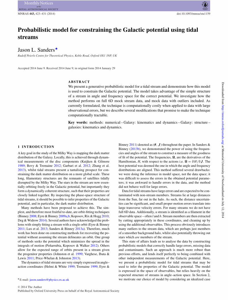
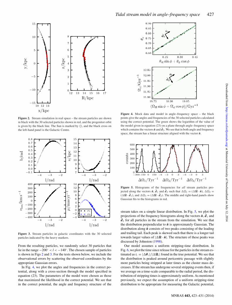
Figure 1. Stream simulation in real space – the stream particles are shownin black with the 30 selected particles shown in red, and the progenitor orbitis given by the black line. The Sun is marked by , and the black cross onthe left-hand panel is the Galactic Centre.

The two parameters of this potential are Vc and q. We setVc = 220 km s−1 and q = 0.9 for the simulation. We place a clusterat the apocentre of the orbit shown in Fig. 1. This orbit was chosendue to its similarity to the orbit of the GD-1 stream (Koposov et al.2010). The orbit has initial conditions (R, z) = (26.0, 0.0) kpc and(U, V, W) = (0.0, 141.8, 83.1) km s−1, where positive U is towardsthe Galactic Centre and positive V is in the direction of the Galacticrotation at the Sun. We seed the simulation with 10 000 particlesdrawn from a 2 × 104M King profile with the ratio of centralpotential to squared-velocity parameter, W0 = 0/σ

2 = 2, a tidallimiting radius, rt ≈ 70 pc, and a King core radius of ≈20 pc. Weevolve the simulation for t ≈ 4.2 Gyr (until just after 11th pericentrepassage of the progenitor) using the code GYRFALCON (Dehnen 2000,2002).

We take the resulting distribution of particles, remove the progen-itor remnant with a spatial cut, and rotate the coordinate frame suchthat the Sun is placed at the same azimuthal angle as the progenitor.

MNRAS 443, 423–431 (2014)

at Mem

orial University of N

ewfoundland on July 12, 2014

http://mnras.oxfordjournals.org/

Dow

nloaded from

Tidal stream model in angle–frequency space 427

Figure 2. Stream simulation in real space – the stream particles are shownin black with the 30 selected particles shown in red, and the progenitor orbitis given by the black line. The Sun is marked by , and the black cross onthe left-hand panel is the Galactic Centre.

Figure 3. Stream particles in galactic coordinates with the 30 selectedparticles indicated by the heavy markers.

From the resulting particles, we randomly select 30 particles thatlie in the range −200◦ < l < −140◦. The chosen sample of particlesis shown in Figs 2 and 3. For the tests shown below, we include theobservational errors by scattering the observed coordinates by theappropriate Gaussian errors.

In Fig. 4, we plot the angles and frequencies in the correct po-tential, along with a cross-section through the model specified inequation (23). The parameters of the model were chosen as thosethat maximized the likelihood in the correct potential. We see thatin the correct potential, the angle and frequency structure of the

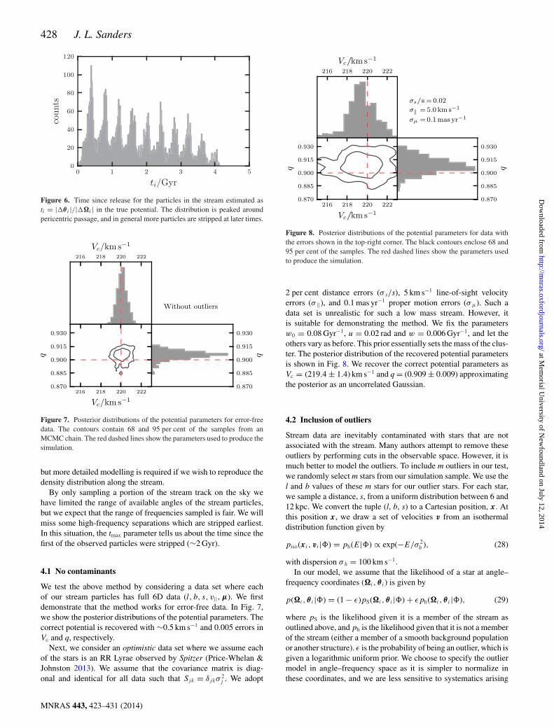
Figure 4. Mock data and model in angle–frequency space – the blackpoints give the angles and frequencies of the 30 selected particles calculatedusing the correct potential. The green shows the logarithm of the value ofthe model given in equation (23) on a plane through angle–frequency spacewhich contains the vectors n and d2. We see that in both angle and frequencyspace, the stream has a linear structure aligned with the vector n.

Figure 5. Histograms of the frequencies for all stream particles pro-jected along the vectors n, d1 and d2 such that �1 = (�� · n), �2 =(�� · d1), and �3 = (�� · d2). The middle and right-hand panels showGaussian fits to the histograms in red.

stream takes on a simple linear distribution. In Fig. 5, we plot theprojections of the frequency histograms along the vectors n, d1 andd2 for all particles in the stream from the simulation. We see thatthe distribution perpendicular to n is approximately Gaussian. Thedistribution along n consists of two peaks consisting of the leadingand trailing tail. Each peak is skewed such that there is a longer tailtowards larger values of |�� · n|. The structure of these peaks wasdiscussed by Johnston (1998).

Our model assumes a uniform stripping-time distribution. InFig. 6, we plot the time since release for the particles in the stream es-timated as ti = |�θ i |/|��i | found in the true potential. We see thatthe distribution is peaked around pericentric passage with slightlymore particles being stripped at later times as the cluster mass de-creases. If the stream has undergone several stripping events then, ifwe average on a time-scale comparable to the radial period, the dis-tribution of stripping times is approximately uniform. As mentionedpreviously, we expect the assumption of a uniform stripping-timedistribution to be appropriate for measuring the Galactic potential,

MNRAS 443, 423–431 (2014)

at Mem

orial University of N

ewfoundland on July 12, 2014

http://mnras.oxfordjournals.org/

Dow

nloaded from

428 J. L. Sanders

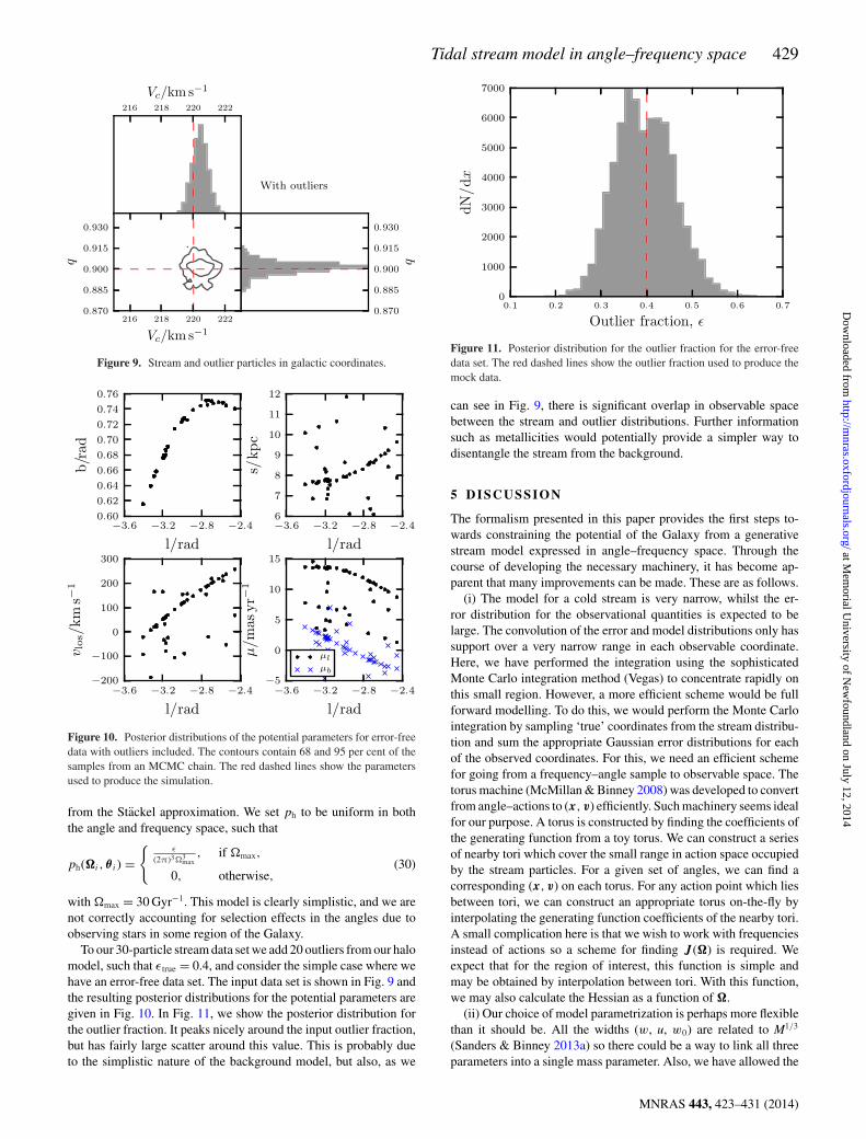
Figure 6. Time since release for the particles in the stream estimated asti = |�θ i |/|��i | in the true potential. The distribution is peaked aroundpericentric passage, and in general more particles are stripped at later times.

Figure 7. Posterior distributions of the potential parameters for error-freedata. The contours contain 68 and 95 per cent of the samples from anMCMC chain. The red dashed lines show the parameters used to produce thesimulation.

but more detailed modelling is required if we wish to reproduce thedensity distribution along the stream.

By only sampling a portion of the stream track on the sky wehave limited the range of available angles of the stream particles,but we expect that the range of frequencies sampled is fair. We willmiss some high-frequency separations which are stripped earliest.In this situation, the tmax parameter tells us about the time since thefirst of the observed particles were stripped (∼2 Gyr).

4.1 No contaminants

We test the above method by considering a data set where eachof our stream particles has full 6D data (l, b, s, v||, μ). We firstdemonstrate that the method works for error-free data. In Fig. 7,we show the posterior distributions of the potential parameters. Thecorrect potential is recovered with ∼0.5 km s−1 and 0.005 errors inVc and q, respectively.

Next, we consider an optimistic data set where we assume eachof the stars is an RR Lyrae observed by Spitzer (Price-Whelan &Johnston 2013). We assume that the covariance matrix is diag-onal and identical for all data such that Sjk = δjkσ

2j . We adopt

Figure 8. Posterior distributions of the potential parameters for data withthe errors shown in the top-right corner. The black contours enclose 68 and95 per cent of the samples. The red dashed lines show the parameters usedto produce the simulation.

2 per cent distance errors (σ s/s), 5 km s−1 line-of-sight velocityerrors (σ ||), and 0.1 mas yr−1 proper motion errors (σμ). Such adata set is unrealistic for such a low mass stream. However, itis suitable for demonstrating the method. We fix the parametersw0 = 0.08 Gyr−1, u = 0.02 rad and w = 0.006 Gyr−1, and let theothers vary as before. This prior essentially sets the mass of the clus-ter. The posterior distribution of the recovered potential parametersis shown in Fig. 8. We recover the correct potential parameters asVc = (219.4 ± 1.4) km s−1 and q = (0.909 ± 0.009) approximatingthe posterior as an uncorrelated Gaussian.

4.2 Inclusion of outliers

Stream data are inevitably contaminated with stars that are notassociated with the stream. Many authors attempt to remove theseoutliers by performing cuts in the observable space. However, it ismuch better to model the outliers. To include m outliers in our test,we randomly select m stars from our simulation sample. We use thel and b values of these m stars for our outlier stars. For each star,we sample a distance, s, from a uniform distribution between 6 and12 kpc. We convert the tuple (l, b, s) to a Cartesian position, x. Atthis position x, we draw a set of velocities v from an isothermaldistribution function given by

piso(xi , vi |�) = ph(E|�) ∝ exp(−E/σ 2h ), (28)

with dispersion σ h = 100 km s−1.In our model, we assume that the likelihood of a star at angle–

frequency coordinates (�i , θ i) is given by

p(�i , θ i |�) = (1 − ε)pS(�i , θ i |�) + εph(�i , θ i |�), (29)

where pS is the likelihood given it is a member of the stream asoutlined above, and ph is the likelihood given that it is not a memberof the stream (either a member of a smooth background populationor another structure). ε is the probability of being an outlier, which isgiven a logarithmic uniform prior. We choose to specify the outliermodel in angle–frequency space as it is simpler to normalize inthese coordinates, and we are less sensitive to systematics arising

MNRAS 443, 423–431 (2014)

at Mem

orial University of N

ewfoundland on July 12, 2014

http://mnras.oxfordjournals.org/

Dow

nloaded from

Tidal stream model in angle–frequency space 429

Figure 9. Stream and outlier particles in galactic coordinates.

Figure 10. Posterior distributions of the potential parameters for error-freedata with outliers included. The contours contain 68 and 95 per cent of thesamples from an MCMC chain. The red dashed lines show the parametersused to produce the simulation.

from the Stackel approximation. We set ph to be uniform in boththe angle and frequency space, such that

ph(�i , θ i) ={

ε

(2π)33max

, if max,

0, otherwise,(30)

with max = 30 Gyr−1. This model is clearly simplistic, and we arenot correctly accounting for selection effects in the angles due toobserving stars in some region of the Galaxy.

To our 30-particle stream data set we add 20 outliers from our halomodel, such that εtrue = 0.4, and consider the simple case where wehave an error-free data set. The input data set is shown in Fig. 9 andthe resulting posterior distributions for the potential parameters aregiven in Fig. 10. In Fig. 11, we show the posterior distribution forthe outlier fraction. It peaks nicely around the input outlier fraction,but has fairly large scatter around this value. This is probably dueto the simplistic nature of the background model, but also, as we

Figure 11. Posterior distribution for the outlier fraction for the error-freedata set. The red dashed lines show the outlier fraction used to produce themock data.

can see in Fig. 9, there is significant overlap in observable spacebetween the stream and outlier distributions. Further informationsuch as metallicities would potentially provide a simpler way todisentangle the stream from the background.

5 D I SCUSSI ON

The formalism presented in this paper provides the first steps to-wards constraining the potential of the Galaxy from a generativestream model expressed in angle–frequency space. Through thecourse of developing the necessary machinery, it has become ap-parent that many improvements can be made. These are as follows.

(i) The model for a cold stream is very narrow, whilst the er-ror distribution for the observational quantities is expected to belarge. The convolution of the error and model distributions only hassupport over a very narrow range in each observable coordinate.Here, we have performed the integration using the sophisticatedMonte Carlo integration method (Vegas) to concentrate rapidly onthis small region. However, a more efficient scheme would be fullforward modelling. To do this, we would perform the Monte Carlointegration by sampling ‘true’ coordinates from the stream distribu-tion and sum the appropriate Gaussian error distributions for eachof the observed coordinates. For this, we need an efficient schemefor going from a frequency–angle sample to observable space. Thetorus machine (McMillan & Binney 2008) was developed to convertfrom angle–actions to (x, v) efficiently. Such machinery seems idealfor our purpose. A torus is constructed by finding the coefficients ofthe generating function from a toy torus. We can construct a seriesof nearby tori which cover the small range in action space occupiedby the stream particles. For a given set of angles, we can find acorresponding (x, v) on each torus. For any action point which liesbetween tori, we can construct an appropriate torus on-the-fly byinterpolating the generating function coefficients of the nearby tori.A small complication here is that we wish to work with frequenciesinstead of actions so a scheme for finding J(�) is required. Weexpect that for the region of interest, this function is simple andmay be obtained by interpolation between tori. With this function,we may also calculate the Hessian as a function of �.

(ii) Our choice of model parametrization is perhaps more flexiblethan it should be. All the widths (w, u, w0) are related to M1/3

(Sanders & Binney 2013a) so there could be a way to link all threeparameters into a single mass parameter. Also, we have allowed the

MNRAS 443, 423–431 (2014)

at Mem

orial University of N

ewfoundland on July 12, 2014

http://mnras.oxfordjournals.org/

Dow

nloaded from

430 J. L. Sanders

stream to be oriented along some random direction, n. The directiondepends on the exact structure of the action distribution, and thestructure of the Hessian matrix. The first of these can be sensitiveto internal structure in the progenitor. We gain information about nthrough the use of the angle and frequency structure as discussed inSanders & Binney (2013b). However, we could instead choose tomake n a function of the progenitor actions in the chosen potential.This would constrain the models in a more physically motivatedfashion, and would provide more information when the quality ofthe data is reduced.

(iii) We have analysed a simulated stream evolved in a near-spherical logarithmic potential. As discussed in Sanders & Binney(2013a), this does not exhibit substantial offset between the streamand orbit tracks. Such an offset is more apparent in flattened po-tentials. Therefore, more tests are required with more realistic po-tentials with disc components to validate the modelling approachpresented here. Additionally, our potential has only two parameters,whilst, in a practical application, a more flexible potential modelshould be adopted. We have found that the parameters of this two-parameter potential are recovered without significant correlations.From stream data, we are measuring the acceleration in some smallspatial volume which in the axisymmetric case is given approxi-mately by the gradients d�/dR and d�/dz at the progenitor. Thesegradients uniquely specify a combination of Vc and q. However,with more parameters in our potential model, many combinationsof these parameters would give identical accelerations at the pro-genitor, so strong correlations are to be expected. More work isrequired to say exactly what properties of the potential, and hencewhat potential parameter combinations, a given set of stream databest measures.

(iv) The distributions in frequency and angle, Ki, along the prin-cipal stream direction, n, were taken in this paper to be simpleGaussians and a uniform distribution. This procedure is adequate forour purposes but more realistic distributions are required to repro-duce the peaky distribution from Fig. 6, and the expected featheringin the stream (Kupper, Lane & Heggie 2012; Sanders & Binney2013b). For instance, a first step would be to adjust the distributionover stripping times to be more concentrated around pericentricpassage of the progenitor by modelling p(ti) as a comb of Gaussiansseparated by the radial period of the progenitor model. However,for measuring the Galactic potential, the shape of the stream is farmore important than the density along the stream and, as we haveshown, the assumption of a uniform stripping-time distribution issufficient for recovery of the potential parameters.Recently Bovy (2014) presented a machinery very similar to thatshown here for constructing models of tidal streams. He exploitsthe narrow range of frequencies in the stream to construct a simplelinear map between (�, θ ) and (x, v). The Gaussian structure in(�, θ ) space can then be simply translated into a Gaussian structurein (x, v) making marginalization over missing data simpler. Helmi& White (1999) present a similar approach to analysing a streammodel consisting of a Gaussian structure in action space and initialangle space.

6 C O N C L U S I O N S

We have presented a probabilistic model for a tidal stream and usedthis to constrain the potential from a simulation. The stream modelbuilds on the work of Sanders & Binney (2013b) by constructinga simple model for the stream in frequency and angle space. Thepresented formalism naturally accounts for the errors in stream data,and can also incorporate the possibility of stream data being con-

taminated with stars from a smooth halo population or another tidalstructure. We have successfully recovered the potential parametersused to run an N-body simulation of a GD-1-like stream from error-free data, data with small errors included, and data with outliersincluded.

As currently formulated, the computational cost of implement-ing our approach increases significantly with the magnitude of theobservational errors. We have described modifications that promiseto mitigate this effect, and thus to make the approach a powerfultechnique for constraining the Galaxy’s gravitational potential.

AC K N OW L E D G E M E N T S

JLS thanks James Binney, Hans-Walter Rix, David Hogg, PaulMcMillan and the dynamics group in Oxford for useful conver-sations which shaped this work. JLS acknowledges the support ofthe Science and Technology Facilities Council, and the commentsfrom the anonymous referee which improved this work.

R E F E R E N C E S

Binney J., 2008, MNRAS, 386, L47Bovy J., 2014, preprint (arXiv:e-prints)Bovy J., Tremaine S., 2012, ApJ, 756, 89Deg N., Widrow L., 2014, , MNRAS, 439, 2678Dehnen W., 2000, ApJ, 536, L39Dehnen W., 2002, J. Comput. Phys., 179, 27Eyre A., 2010, DPhil thesis, Univ. Oxford, OxfordEyre A., Binney J., 2009a, MNRAS, 399, L160Eyre A., Binney J., 2009b, MNRAS, 400, 548Eyre A., Binney J., 2011, MNRAS, 413, 1852Foreman-Mackey D., Hogg D. W., Lang D., Goodman J., 2013, PASP, 125,

306Galassi M., Davies J., Theiler J., Gough B., Jungman G., 2009, GNU Scien-

tific Library - Reference Manual, Third Edition, for GSL Version 1.12.Network Theory Ltd, p. 1

Garbari S., Liu C., Read J. I., Lake G., 2012, MNRAS, 425, 1445Helmi A., White S. D. M., 1999, MNRAS, 307, 495Johnston K. V., 1998, ApJ, 495, 297Johnston K. V., Zhao H. S., Spergel D. N., Hernquist L., 1999, in Unwin

S., Stachnik R., eds, ASP Conf. Ser. Vol. 194, Working on the Fringe:Optical and IR Interferometry from Ground and Space. Astron. Soc.Pac., San Francisco, p. 15

Koposov S. E., Rix H.-W., Hogg D. W., 2010, ApJ, 712, 260Kuijken K., Gilmore G., 1989, MNRAS, 239, 605Kupper A. H. W., Lane R. R., Heggie D. C., 2012, MNRAS, 420, 2700Lepage G. P., 1978, J. Comput. Phys., 27, 192Lux H., Read J. I., Lake G., Johnston K. V., 2013, MNRAS, 436, 2386McMillan P. J., Binney J. J., 2008, MNRAS, 390, 429Penarrubia J., Koposov S. E., Walker M. G., 2012, ApJ, 760, 2Price-Whelan A. M., Johnston K. V., 2013, ApJ, 778, L12Sanders J., 2012, MNRAS, 426, 128Sanders J. L., Binney J., 2013a, MNRAS, 433, 1813Sanders J. L., Binney J., 2013b, MNRAS, 433, 1826Tremaine S., 1999, MNRAS, 307, 877Varghese A., Ibata R., Lewis G. F., 2011, MNRAS, 417, 198Zhang L., Rix H.-W., van de Ven G., Bovy J., Liu C., Zhao G., 2013, ApJ,

772, 108

A P P E N D I X A : C A L C U L AT I N G T H E H E S S I A N

As part of our likelihood in Section 2, we require the Hessian matrix,D = ∂2H/∂ J2. In a Stackel potential, this matrix may be foundnumerically by following the procedure presented in the Appendixof Eyre (2010). This involves finding the second derivatives of

MNRAS 443, 423–431 (2014)

at Mem

orial University of N

ewfoundland on July 12, 2014

http://mnras.oxfordjournals.org/

Dow

nloaded from

Tidal stream model in angle–frequency space 431

the analytic integral expressions for the actions with respect to theintegrals of motion: the energy, E, the z-component of the angularmomentum, Lz, and the third integral, I3. The resulting integrals areperformed analytically using Gaussian quadrature, but care must betaken due to the divergence of the frequency integrand at the endpoints. These considerations are taken care of by introduction of adummy variable as described in Eyre (2010).

For our purposes, we are using a Stackel approximation to thetrue potential (Sanders 2012) so we estimate the true Hessian matrixas that calculated in the approximate Stackel potential. In the truepotential, the error in each component of the Hessian matrix is lessthan 10 per cent. However, the error in the determinant is larger(∼30 per cent). As the potentials considered are near-spherical, thedeterminant of the Hessian is small (it is zero for the spherical case),which arises due to cancelling terms in the calculation. Therefore,

small errors in each component can give rise to larger errors in thedeterminant. We recover the appropriate trends in the determinant ofthe Hessian matrix with the potential parameters. There is a slightbias in Fig. 7 which is probably due to the errors in the Hessianmatrix. However, it is not significant. The results shown in thispaper demonstrate that the magnitude of the observational errors inthe data dominates any systematic errors in estimating the angles,frequencies, or the determinant of the Hessian matrix.

A better, but more time-consuming, estimate of the Hessian ma-trix may be found using the torus machine (McMillan & Binney2008) as described in Sanders & Binney (2013a).

This paper has been typeset from a TEX/LATEX file prepared by the author.

MNRAS 443, 423–431 (2014)

at Mem

orial University of N

ewfoundland on July 12, 2014

http://mnras.oxfordjournals.org/

Dow

nloaded from