Probability: The Foundation of Inferential Statistics

October 14, 2009

Subjective Probability

• Throughout the course I have used the word probability.– Yet I have not defined it. Instead I have relied on

the assumption that you all have a sense of probability.

– The book calls this sense of probability “subjective probability”.

Classical Approach to Probability

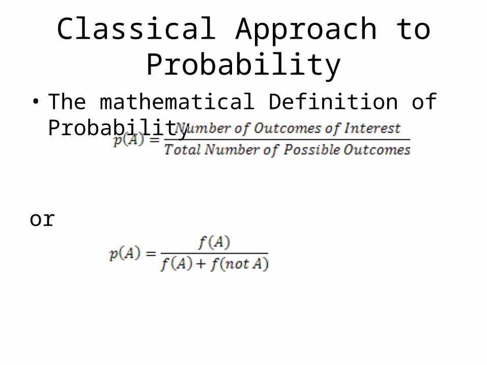
• The mathematical Definition of Probability

or

Empirical Approach to Probability

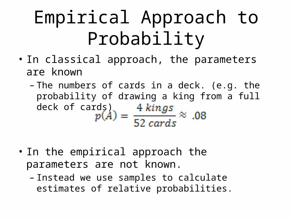
• In classical approach, the parameters are known– The numbers of cards in a deck. (e.g. the probability

of drawing a king from a full deck of cards)

• In the empirical approach the parameters are not known.– Instead we use samples to calculate estimates of

relative probabilities.

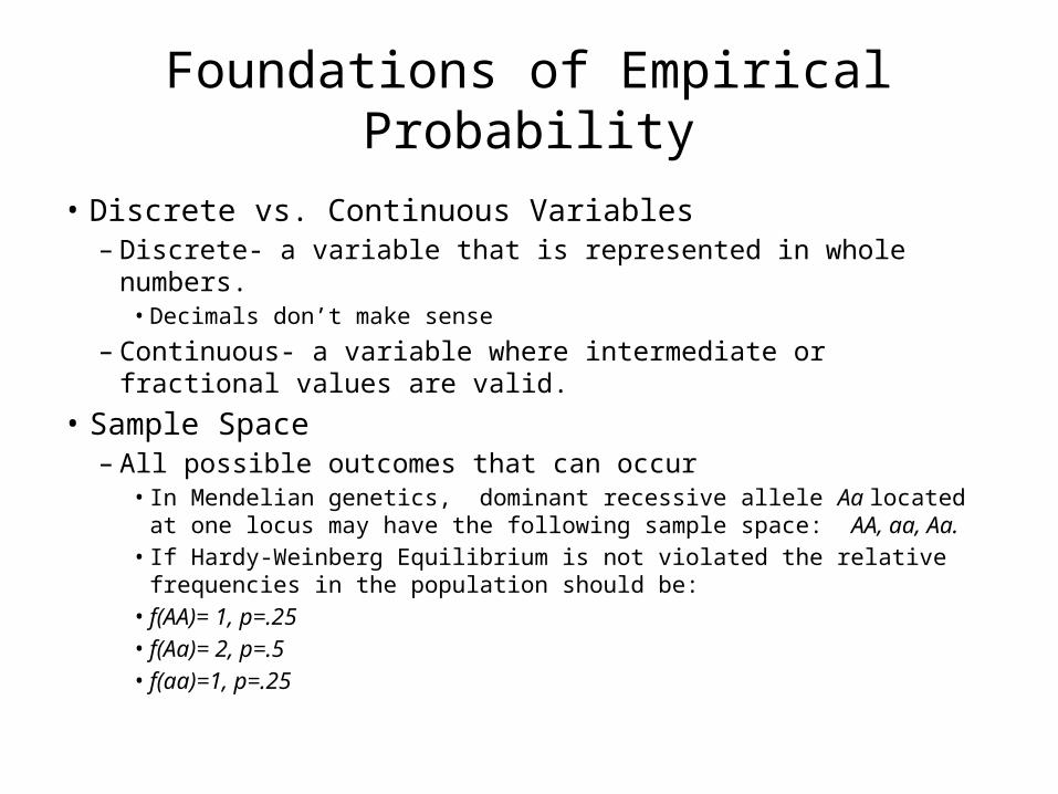
Foundations of Empirical Probability

• Discrete vs. Continuous Variables– Discrete- a variable that is represented in whole numbers.

• Decimals don’t make sense

– Continuous- a variable where intermediate or fractional values are valid.

• Sample Space– All possible outcomes that can occur

• In Mendelian genetics, dominant recessive allele Aa located at one locus may have the following sample space: AA, aa, Aa.

• If Hardy-Weinberg Equilibrium is not violated the relative frequencies in the population should be:

• f(AA)= 1, p=.25• f(Aa)= 2, p=.5• f(aa)=1, p=.25

Mutually vs. Nonmutually Exclusive Events

• Mutually Exclusive– Events in our sample that cannot occur together

or overlap.• Nonmutually exclusive events– Events in our sample that can occur together.– A joint probability is the degree in which a set of

events do occur together in a sample.

Calculating Probability

• Probability can be expressed – in a percentage or relative frequency in 100. – As a decimal. • p= .5 is the same as, 50% chance, is the same as saying

50 in one hundred.

• The addition rule: p(A or B)– It is used when we want to calculate the

probability of selecting an element that has one or more conditions.

Calculating Probability

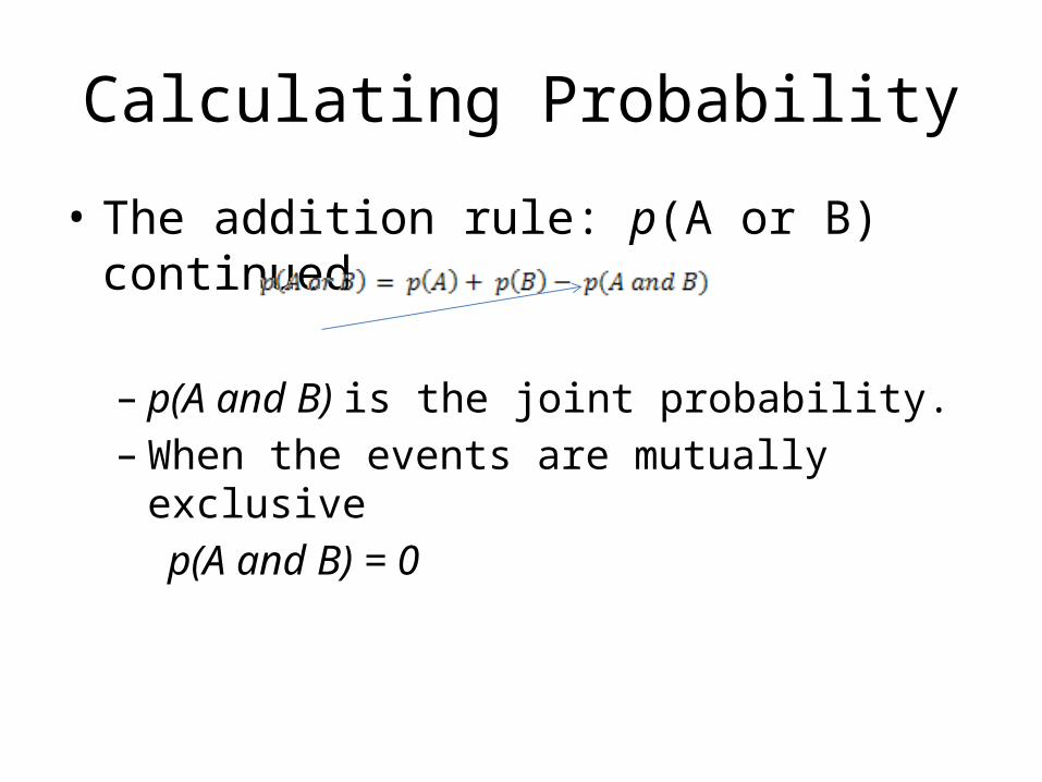
• The addition rule: p(A or B) continued

– p(A and B) is the joint probability.– When the events are mutually exclusive p(A and B) = 0

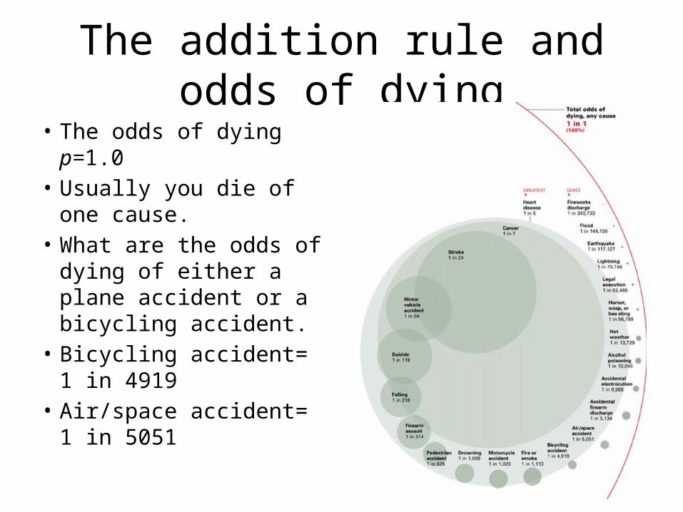
The addition rule and odds of dying• The odds of dying p=1.0• Usually you die of one

cause.• What are the odds of

dying of either a plane accident or a bicycling accident.

• Bicycling accident= 1 in 4919

• Air/space accident= 1 in 5051

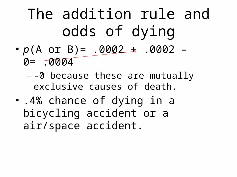
The addition rule and odds of dying

• p(A or B)= .0002 + .0002 – 0= .0004 – -0 because these are mutually exclusive causes of

death. • .4% chance of dying in a bicycling accident or a

air/space accident.

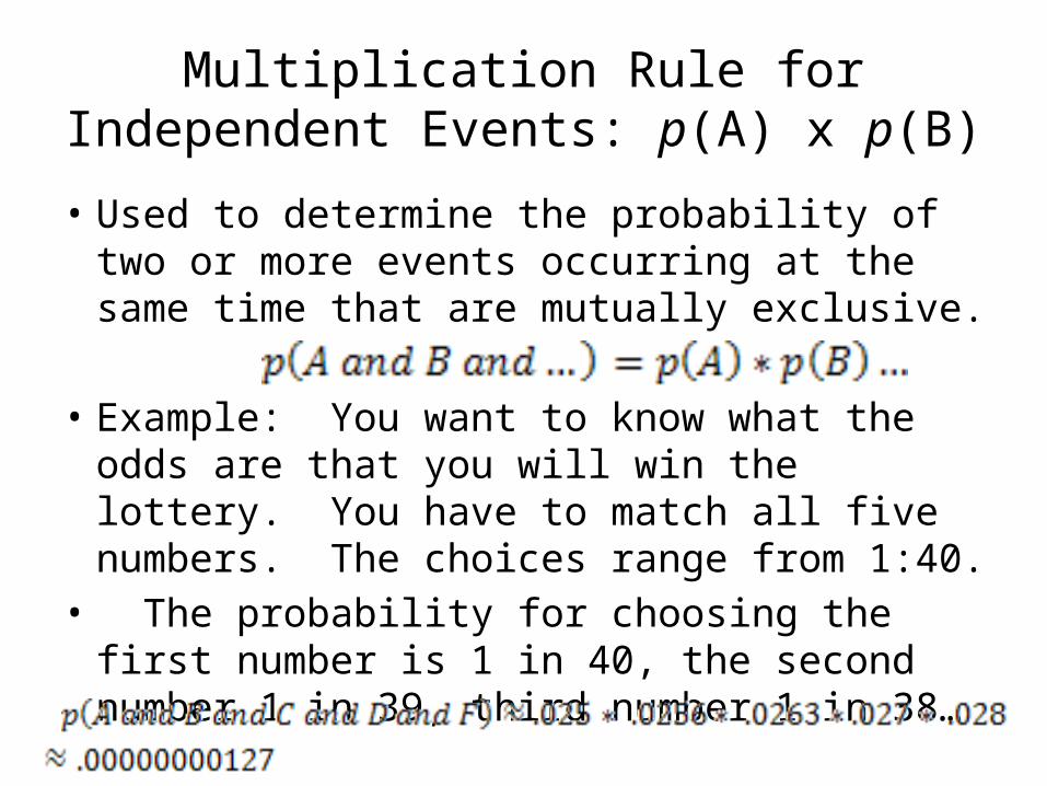
Multiplication Rule for Independent Events: p(A) x p(B)

• Used to determine the probability of two or more events occurring at the same time that are mutually exclusive.

• Example: You want to know what the odds are that you will win the lottery. You have to match all five numbers. The choices range from 1:40.

• The probability for choosing the first number is 1 in 40, the second number 1 in 39, third number 1 in 38…

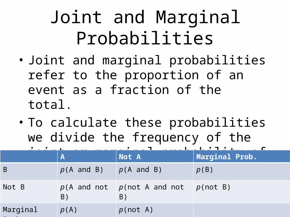
Joint and Marginal Probabilities

• Joint and marginal probabilities refer to the proportion of an event as a fraction of the total.

• To calculate these probabilities we divide the frequency of the joint or marginal probability of two or more events by the total frequency.

A Not A Marginal Prob.

B p(A and B) p(A and B) p(B)

Not B p(A and not B) p(not A and not B) p(not B)

Marginal Prob. p(A) p(not A)

Calculating ProbabilitiesA Not A Marginal Prob.

B p=f(A and B)/tot p=f(A and B)/tot p(B)= f(B)/Total

Not B p=f(A and not B)/tot p=f(not A and not B)/tot p(not B)= f(not B)/Total

Marginal Prob.

p(A)= f(A)/Total p(not A)= f(not A)/Total total/total= 1.00

•The previous graph just gave you where the different types of probabilities are located on the chart. •This chart gives you the way you would calculate these probabilites.•You will be given a frequency for each cell (e.g. B= 20, not B=80, A= 48, not A= 52)•With this information you should be able to create a similar chart.

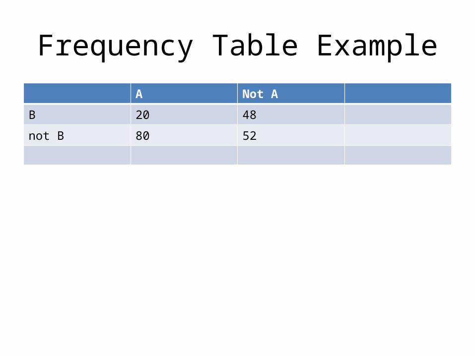
Frequency Table ExampleA Not A

B 20 48

not B 80 52

Frequency Table ExampleA Not A Marginal

ProbabilityB 20 48 = 20 +48

not B 80 52 = 80 + 52

Marginal Probability =20 + 80 =48 +52

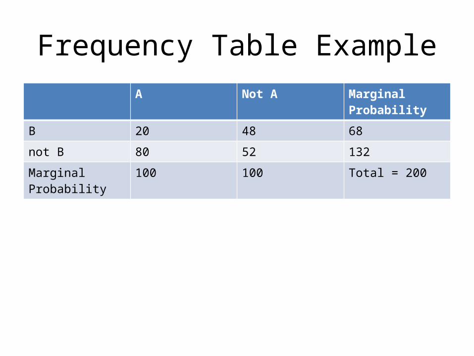
Frequency Table ExampleA Not A Marginal

ProbabilityB 20 48 68

not B 80 52 132

Marginal Probability 100 100 Total = 200

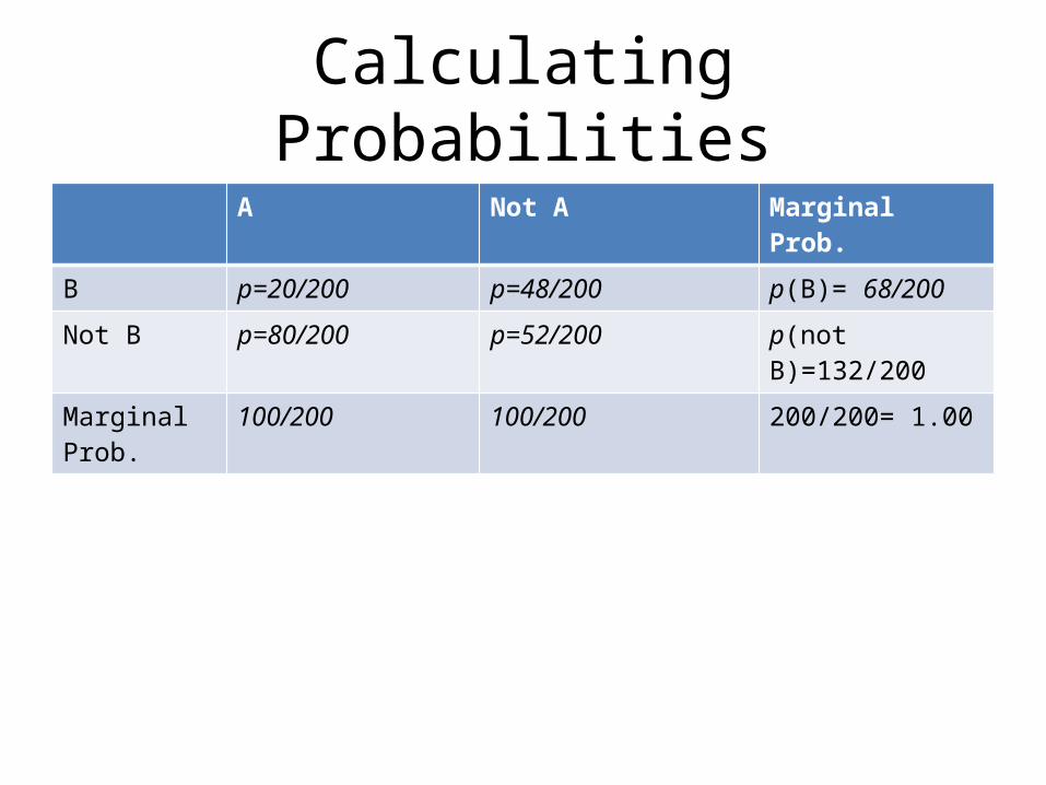
Calculating ProbabilitiesA Not A Marginal Prob.

B p=20/200 p=48/200 p(B)= 68/200

Not B p=80/200 p=52/200 p(not B)=132/200

Marginal Prob.

100/200 100/200 200/200= 1.00

Calculating ProbabilitiesA Not A Marginal Prob.

B p(A and B)=.1 p(not A and B)=.24 p(B)= .34

Not B p(A and not B)=.4 p(not A and not B)=.26 p(not B)=.66

Marginal Prob.

p(A)=.5 p(A).5 200/200= 1.00

Conditional ProbabilitiesA Not A

B

(not B)

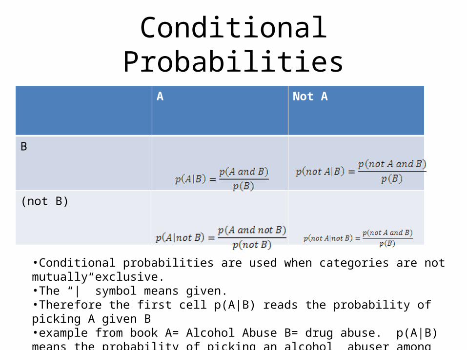
•Conditional probabilities are used when categories are not mutually exclusive.•The “|” symbol means given. •Therefore the first cell p(A|B) reads the probability of picking A given B•example from book A= Alcohol Abuse B= drug abuse. p(A|B) means the probability of picking an alcohol abuser among drug abusers.

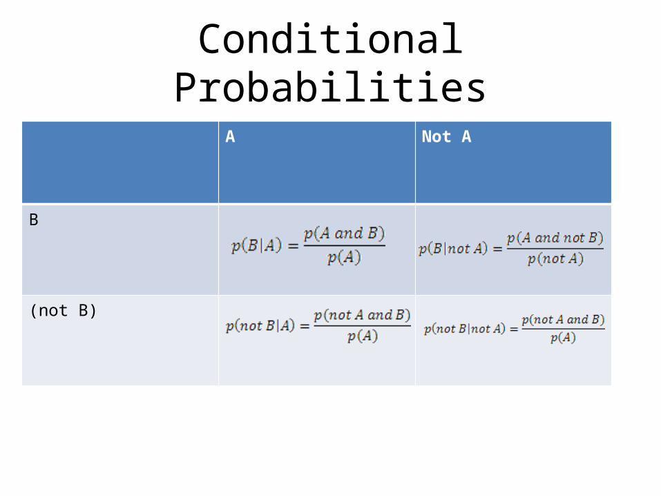
Conditional ProbabilitiesA Not A

B

(not B)

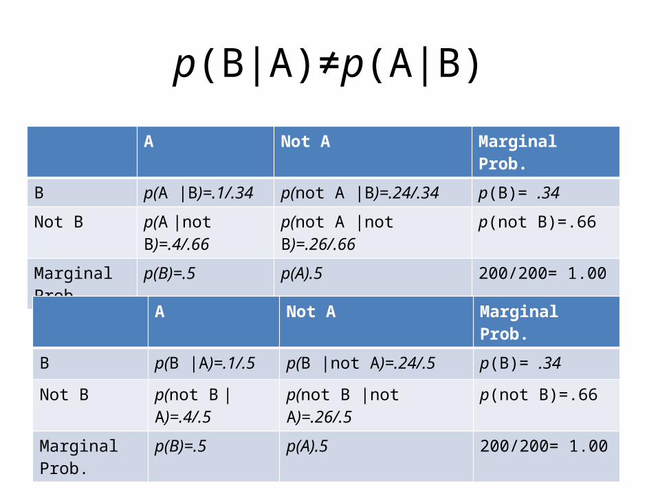
p(B|A)≠p(A|B)

A Not A Marginal Prob.

B p(A |B)=.1/.34 p(not A |B)=.24/.34 p(B)= .34

Not B p(A |not B)=.4/.66 p(not A |not B)=.26/.66 p(not B)=.66

Marginal Prob.

p(B)=.5 p(A).5 200/200= 1.00

A Not A Marginal Prob.

B p(B |A)=.1/.5 p(B |not A)=.24/.5 p(B)= .34

Not B p(not B |A)=.4/.5 p(not B |not A)=.26/.5 p(not B)=.66

Marginal Prob. p(B)=.5 p(A).5 200/200= 1.00

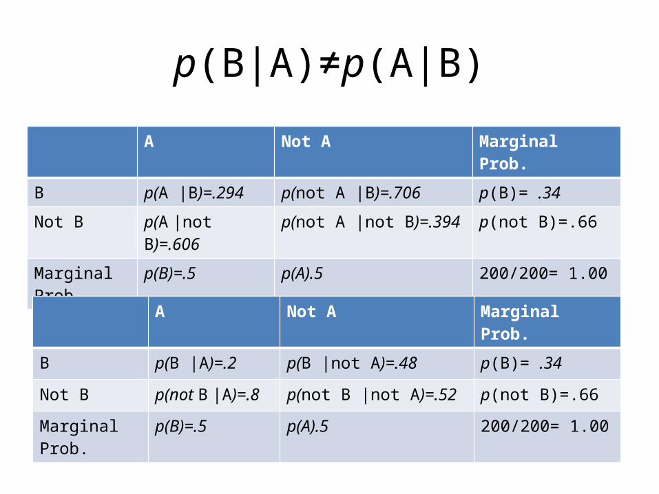
p(B|A)≠p(A|B)

A Not A Marginal Prob.

B p(A |B)=.294 p(not A |B)=.706 p(B)= .34

Not B p(A |not B)=.606 p(not A |not B)=.394 p(not B)=.66

Marginal Prob.

p(B)=.5 p(A).5 200/200= 1.00

A Not A Marginal Prob.

B p(B |A)=.2 p(B |not A)=.48 p(B)= .34

Not B p(not B |A)=.8 p(not B |not A)=.52 p(not B)=.66

Marginal Prob. p(B)=.5 p(A).5 200/200= 1.00

Determining Joint Probabilites when Conditional and Marginal Probabilities are given

A Not A Marginal Prob.

B p(B |A)=.2 p(B |not A)=.48 p(B)= .34

Not B p(not B |A)=.8 p(not B |not A)=.52 p(not B)=.66

Marginal Prob. p(A)=.5 p(not A).5 200/200= 1.00

A Not A Marginal Prob.

B p(B and A)=.2*.5 p(B and not A)=.48*.5 p(B)= .34

Not B p(not B and A)=.8*.5 p(not B and not A)=.52*.5 p(not B)=.66

Marginal Prob. p(A)=.5 p(not A).5 200/200= 1.00

A Not A Marginal Prob.

B p(A and B)=.1 p(not A and B)=.24 p(B)= .34

Not B p(A and not B)=.4 p(not A and not B)=.26 p(not B)=.66

Marginal Prob. p(A)=.5 p(A).5 200/200= 1.00

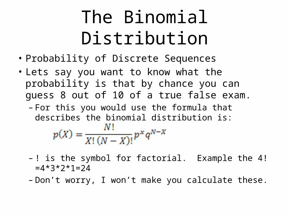
The Binomial Distribution

• Probability of Discrete Sequences• Lets say you want to know what the probability is

that by chance you can guess 8 out of 10 of a true false exam. – For this you would use the formula that describes the

binomial distribution is:

– ! is the symbol for factorial. Example the 4!=4*3*2*1=24– Don’t worry, I won’t make you calculate these.

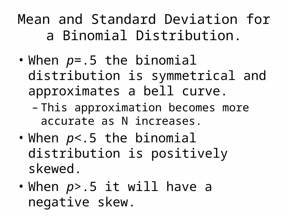
Mean and Standard Deviation for a Binomial Distribution.

• When p=.5 the binomial distribution is symmetrical and approximates a bell curve.– This approximation becomes more accurate as N

increases.• When p<.5 the binomial distribution is

positively skewed.• When p>.5 it will have a negative skew.

The Binomial Distribution Continued.

• The binomial distribution has all the same descriptive statistics we already know.

• Mean, standard deviation, and z scores. • We can use what we already know to relate

this distribution to the normal curve.

Example

• Take the midterms I haven’t passed out yet. • Let’s say that the mean on this test Is

around .9 and has a standard deviation of .2. • What is the probability of picking a person at

random who actually failed the test?

Example Continued

• z=(.6-.9)/.2• z=-1.5• Go to the back of the book and see• area beyond z=.0668• Only a 6.6% chance that you failed the test.

Quiz time.