Embed Size (px)
Citation preview
Problem Solutions
Vehicle Energy and Fuel Consumption
Vehicle Energy Losses and Performance Analysis
Problem 2.1
For a vehicle with mv = 1500 kg, Af · cd = 0.7m2, cr = 0.012, a vehicle speedv = 120 km/h and an acceleration a = 0.027 g, calculate the traction torquerequired at the wheels and the corresponding rotational speed level (tires195/65/15T). Calculate the road slope that is equivalent to that acceleration.
• Solution
Assume ρa = 1.20kg/m3, g = 9.81m/s2.a) Traction torque required at wheels:
Ft = mv · cr · g + 1/2 · ρa ·Af · cd · v2 +mv · a =
= 1500 · 0.012 · 9.81 +1
2· 1.2 · 0.7 ·
(120
3.6
)2
+ 1500 · 0.027 · 9.81 = 1041 N
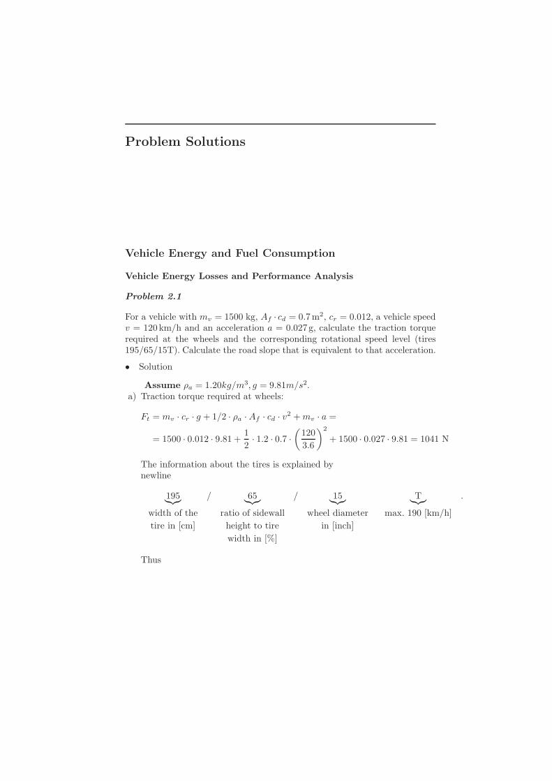
The information about the tires is explained bynewline
195︸︷︷︸width of the
tire in [cm]
/ 65︸︷︷︸ratio of sidewall
height to tire
width in [%]
/ 15︸︷︷︸wheel diameter
in [inch]
T︸︷︷︸max. 190 [km/h]
.
Thus
2 References
rw =dw2
+ hsw =15”
2+ 0.65 · 0.195 = 15 ·
0.0254
2+ 0.65 · 0.195 = 0.317 m
Tt = rw · Ft = 0.317 · 1041 = 330 Nm
b) Rotational speed level:
ωw =v
rw=
120/3.6
0.317· 0.317 = 105.2 rad/s = 1004 rpm
c) Acceleration-equivalent road slope:
α = arcsin((a
g= 0.027) rad
α% = 100 · tan(0.027) = 100 · 0.027 = 2.7 %
For the requested velocity, a traction torque of 330 Nm at a rotational speedof 1004 rpm is required. This is equivalent to the acceleration caused by aslope of 2.7%.
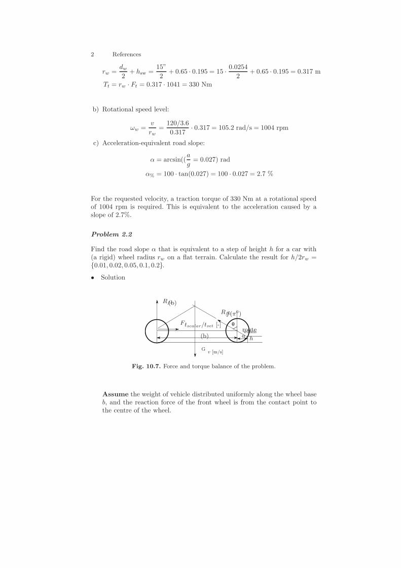
Problem 2.2
Find the road slope α that is equivalent to a step of height h for a car with(a rigid) wheel radius rw on a flat terrain. Calculate the result for h/2rw =0.01, 0.02, 0.05, 0.1, 0.2.
• Solution
θ
G
Rfc
Rfc
(b)
(b)
route
h
F
willans
f(π0)
tscalar/tset [-]
a
v [m/s]
Fig. 10.7. Force and torque balance of the problem.
Assume the weight of vehicle distributed uniformly along the wheel baseb, and the reaction force of the front wheel is from the contact point tothe centre of the wheel.
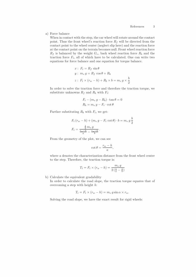
References 3
a) Force balanceWhen in contact with the step, the car wheel will rotate around the contactpoint. Thus the front wheel’s reaction force Rf will be directed from thecontact point to the wheel center (neglect slip here) and the reaction forceat the contact point on the terrain becomes null. Front wheel reaction forceRf is balanced by the weight Gv, back wheel reaction force Rb and thetraction force Ft, all of which have to be calculated. One can write twoequations for force balance and one equation for torque balance.
x : Ft = Rf sin θ
y : mv g = Rf cos θ +Rb
z : Ft × (rw − h) +Rb × b = mv g ×b
2
In order to solve the traction force and therefore the traction torque, wesubstitute unknowns Rf and Rb with Ft:
Ft − (mv g −Rb) · tan θ = 0
Rb = mv g − Ft · cot θ
Further substituting Rb with Ft, we get:
Ft (rw − h) + (mv g − Ft cot θ) · b = mv gb
2
Ft =12 mv g
rw−ha − rw−h
b
.
From the geometry of the plot, we can see
cot θ =rw − h
a,
where a denotes the characterization distance from the front wheel centreto the step. Therefore, the traction torque is:
Tt = Ft × (rw − h) =mv g
2 ( 1a − 1b )
b) Calculate the equivalent gradabilityIn order to calculate the road slope, the traction torque equates that ofovercoming a step with height h:
Tt = Ft × (rw − h) = mv g sinα× rw.
Solving the road slope, we have the exact result for rigid wheels:
4 References
sinα =Ft (rw − h)
mv g rw=
1
2 rw·
ab
b− a
α = arcsin
(ab
2 rw (b− a)
)
=1
2 ( rwa − rwb )
c) Explore a representation of first approximationIf a ≪ b, the solution is no longer correlated with the wheelbase b, whichgives:
α = arcsina
2 rw
Discussion
• Other ways of calculationFrom the geometry, it can be seen that
a2 = r2w − (rw − h)2 = h · (2 rw − h).
Thus, the approximated calculation correlates only one geometric pa-rameter z = h
2·rw:
α = arcsin
⎛
⎝
√hrw
· (2 − hrw
)
4
⎞
⎠
= arcsin
⎛
⎝
√h
2 rw· (1− h
2 rw)
2
⎞
⎠ = arcsin
(√z(1− z)
2
)
Correspondingly, the exact solution correlates the relative height z =h/rw and the relative wheelbase zb = b/rw:
α =1
2 ( rwa − rwb )
=1
2
(1√
2 z(1−z)− 1
zb
)
• Maximum height of the step that can be overcomeNote that the height of the step cannot be larger than the wheel sizez = h
2 rw≤ 1
2 , otherwise the rotation around the contact point maynot be achieved.
• Comparison between the approximated and exact solution:Assume the relative wheelbase b/rw = 6.67, and different relativestep heights as in the Table ??.
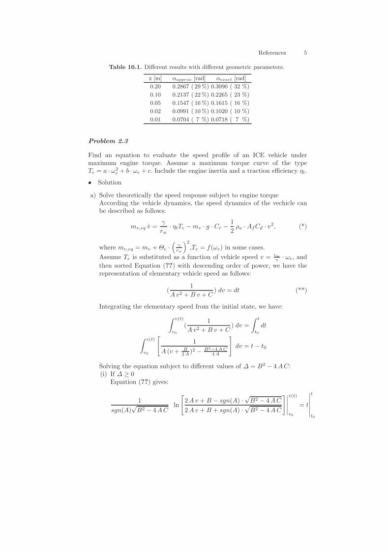
References 5
Table 10.1. Different results with different geometric parameters.
z [m] αapprox [rad] αexact [rad]
0.20 0.2867 ( 29%) 0.3090 ( 32 %)
0.10 0.2137 ( 22%) 0.2265 ( 23 %)
0.05 0.1547 ( 16%) 0.1615 ( 16 %)
0.02 0.0991 ( 10%) 0.1020 ( 10 %)
0.01 0.0704 ( 7 %) 0.0718 ( 7 %)
Problem 2.3
Find an equation to evaluate the speed profile of an ICE vehicle undermaximum engine torque. Assume a maximum torque curve of the typeTe = a · ω2
e + b · ωe + c. Include the engine inertia and a traction efficiency ηt.
• Solution
a) Solve theoretically the speed response subject to engine torqueAccording the vehicle dynamics, the speed dynamics of the vechicle canbe described as follows:
mv,eq v =γ
rw· ηtTe −mv · g · Cr −
1
2ρa · AfCd · v2, (*)
where mv,eq = mv +Θe ·(
γrw
)2,Te = f(ωe) in some cases.
Assume Te is substituted as a function of vehicle speed v = rwγ · ωe, and
then sorted Equation (??) with descending order of power, we have therepresentation of elementary vehicle speed as follows:
(1
Av2 +B v + C) dv = dt (**)
Integrating the elementary speed from the initial state, we have:
∫ v(t)
v0
(1
Av2 +B v + C) dv =
∫ t
t0
dt
∫ v(t)
v0
[1
A (v + B2A )2 − B2−4AC
4A
]
dv = t− t0
Solving the equation subject to different values of ∆ = B2 − 4AC:(i) If ∆ ≥ 0
Equation (??) gives:
1
sgn(A)√B2 − 4AC
ln
[2Av +B − sgn(A) ·
√B2 − 4AC
2Av +B + sgn(A) ·√B2 − 4AC
]∣∣∣∣∣
v(t)
v0
= t
∣∣∣∣∣∣
t
t0
6 References
Let
S+ = sqrtB2 − 4AC
S+ = sgn(A) · sqrtB2 − 4AC
K0 =2Av0 +B − sgn(A) ·
√B2 − 4AC
2Av0 +B + sgn(A) ·√B2 − 4AC
=2Av0 +B − S+
2Av0 +B + S+
,
then, the vehicle speed v can be represented as a explicit function oftime t, when the vehicle starts are v|t0=0 = v0:
K(t) =2Av +B − S+
2Av +B + S+
=2Av0 +B − S+
2Av0 +B + S+
·e[S+(t−t0)] = K0·e[S+(t−t0)]
Equivalently, it can also be represented as
v =S+
2A
1 +K(t)
1−K(t)−
B
2A
=S+[1 +K(t)]−B [1−K(t)]
2A [1−K(t)]
(ii) If ∆ < 0Equation (??) gives:
2
sgn(A) ·√4AC −B2
[arctan
2Av +B
sgn(A)√4AC −B2
− arctan2Av0 +B
sgn(A)√4AC −B2
]= t− t0
Let
S− =√4AC −B2
S− = sgn(A) ·√
4AC −B2,
then, the vehicle speed v can be represented as a explicit function oftime t, when the vehicle starts are v|t0=0 = v0:
arctan2Av + B
S−
− arctan2Av0 +B
S−
=S−
2(t− t0).
Equivalently, it can also be represented as
v =S− · tan
[S−(t−t0)
2 + arctan 2Av0+BS−
]−B
2A
References 7
b) Specific case of maximum torque inputGiven that Te = a · ω2
e + b · ωe + c, the corresponding A,B and C inEquation (??) can be calculated as follows:
A =
(
−1
2· ρa · Af · cd +
(γ
rw
)3
· ηt · a
)
·1
mv,eq
B =
(γ
rw
)2
· ηt · b ·1
mv,eq
C =
(−g ·mv · cr +
γ
rw· ηt · c
)·
1
mv,eq
Finally, substituting these parameters into ∆ and switch to the corre-sponding equations, we can evaluate the speed profile of an ICE vehicleunder maximum engine torque.Discussion• Note that γ/rw generally varies along the acceleration, so a solution
must be obtained step by step.• Specific cases of parameters
(i) Decided by normal shape of maximum torque curveGiven the fact that typical maximum torque curve can be emulatedby a downward parabolar, which means:
a < 0, b ≥ 0, c > 0.
This parameter set gives both possibilities for ∆ to be positive ornegative.
(ii) Decided by different accerleration of vehicleWhen B = 0 and C < 0 (coasting), then D < 0 and one finds back(2.18) for the coasting velocity.
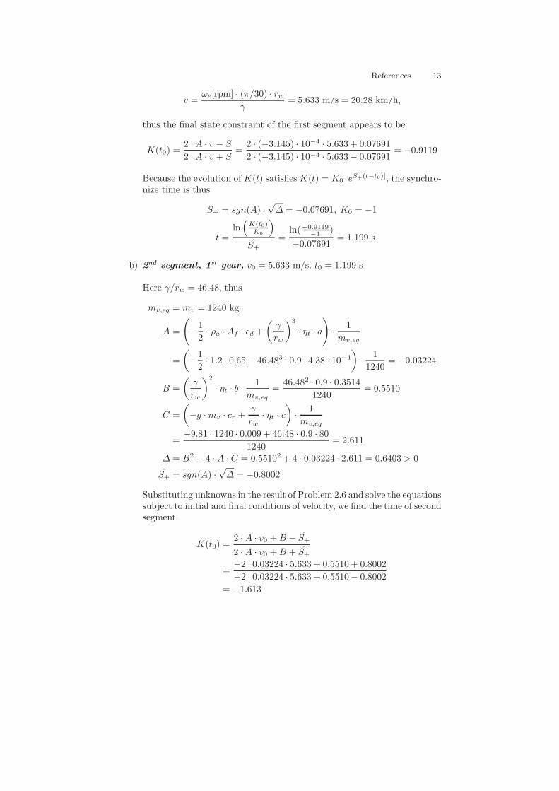
Problem 2.4
Evaluate the 0-100 km/h time precisely using the result of Problem 2.3. Usethe following data: engine launch speed = 2500 rpm, engine upshift speedωe,max = 6500 rpm, γ/rw = 46.48, 29.13, 20.39, 15.04, 11.39, a = −4.38 ·10−4Nms2, b = 0.3514Nms, c = 80Nm, and the following vehicle data:mv = 1240 kg, Af · cd = 0.65 m2, cr = 0.009, ηt = 0.9. Further assume that aslipping clutch transmits all the torque. The momentum of inertia Θe = 0.128kg·m2.
• Solution
a) Estimate gear # at the end of accelerationSince A, B, and C depend on γ, which changes along the speed trajectory,the calculation of v(t) must be separated in segments according to the
8 References
gear and the clutch status. The target speed will be reached in the gear# whose γ/rw is immediately lower than
ωe,max
v=
6500[rpm] · (2 · π/60)100km/h/3.6
= 24.5
Thus the target speed is reached in the third gear. Four segments (includ-ing takeoff) must be considered.
b) Vehicle mass and inertiaAs for the rolling friction, the orignal vehicle mass is used for reactionforce calculation:
mv = 1240kg.
As for the dynamic force, the equivalent mass with engine inertia is con-sidered for each gear #:
mv,eq = mv +Θe ·(γ
rw
)2
c) 1st segment : takeoff, v0 = 0, t0 = 0Although the vehicle is at standstill, the engine is operating at the idlespeed. Using the result of Problem 2.6, we get ωe = 2500 rpm; and sub-stituting torque parameters, we further have:
Te = a · ω2e + b · ωe + c = 142.0 Nm
as a constant torque during slipping-clutch segment.
mv,eq = mv +Θe ·(γ
rw
)2
= 1240 + 0.128 · 46.482 = 1517 kg
A = −1
2· ρa · Af · cd ·
1
mv,eq= −
1
2·1.2 · 0.651517
= −2.571× 10⁻⁴
B = 0
C =
(−g ·mv · cr +
γ
rw· ηt · Te
)·
1
mv,eq=
=−9.81 · 1240 · 0.009 + 46.48 · 0.9 · 142
1517= 3.844
∆ = −4 · A · C > 0
S+ = sgn(A) ·√−4 ·A · C = −1 ·
√4 · 2.571× 10−4 · 3.844 = −0.06287
Substituting unknowns in the result of Problem 2.6 and solve the equationssubject to initial and final conditions of velocity, we find the time of firstsegment.To be more specific, the synchronization time between the engine and thevehicle (clutch closed) is when
References 9
v =ωe[rpm] · (π/30) · rw
γ= 5.633 m/s = 20.28 km/h,
thus the final state constraint of the first segment appears to be:
K(t0) =2 · A · v − S
2 · A · v + S=
2 · (−2.571) · 10−4 · 5.633 + 0.06287
2 · (−2.571) · 10−4 · 5.633− 0.06287= −0.9119
Because the evolution of K(t) satisfies K(t) = K0 ·eS+(t−t0)], the synchro-nize time is thus
S+ = sgn(A) ·√∆ = −0.06287, K0 = −1
t =ln(
K(t0)K0
)
S+
=ln(−0.9119
−1 )
−0.06287= 1.467 s
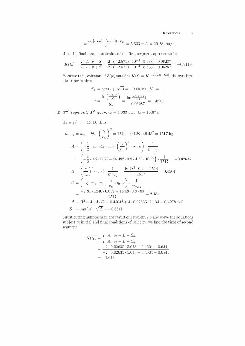
d) 2nd segment, 1st gear, v0 = 5.633 m/s, t0 = 1.467 s
Here γ/rw = 46.48, thus
mv,eq = mv +Θe ·(γ
rw
)2
= 1240 + 0.128 · 46.482 = 1517 kg
A =
(
−1
2· ρa ·Af · cd +
(γ
rw
)3
· ηt · a
)
·1
mv,eq
=
(−1
2· 1.2 · 0.65− 46.483 · 0.9 · 4.38 · 10−4
)·
1
1517= −0.02635
B =
(γ
rw
)2
· ηt · b ·1
mv,eq=
46.482 · 0.9 · 0.35141517
= 0.4504
C =
(−g ·mv · cr +
γ
rw· ηt · c
)·
1
mv,eq
=−9.81 · 1240 · 0.009 + 46.48 · 0.9 · 80
1517= 2.134
∆ = B2 − 4 · A · C = 0.45042 + 4 · 0.02635 · 2.134 = 0.4278 > 0
S+ = sgn(A) ·√∆ = −0.6541
Substituting unknowns in the result of Problem 2.6 and solve the equationssubject to initial and final conditions of velocity, we find the time of secondsegment.
K(t0) =2 · A · v0 +B − S+
2 · A · v0 +B + S+
=−2 · 0.02635 · 5.633 + 0.4504 + 0.6541
−2 · 0.02635 · 5.633 + 0.4504− 0.6541= −1.613
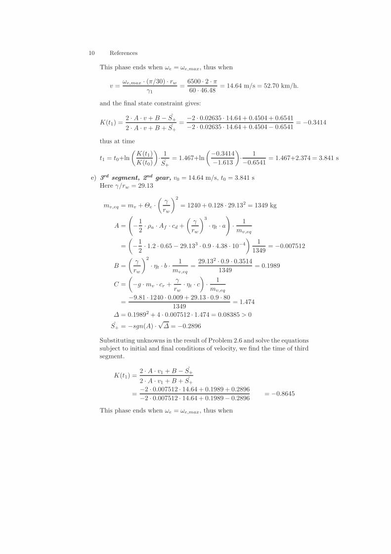
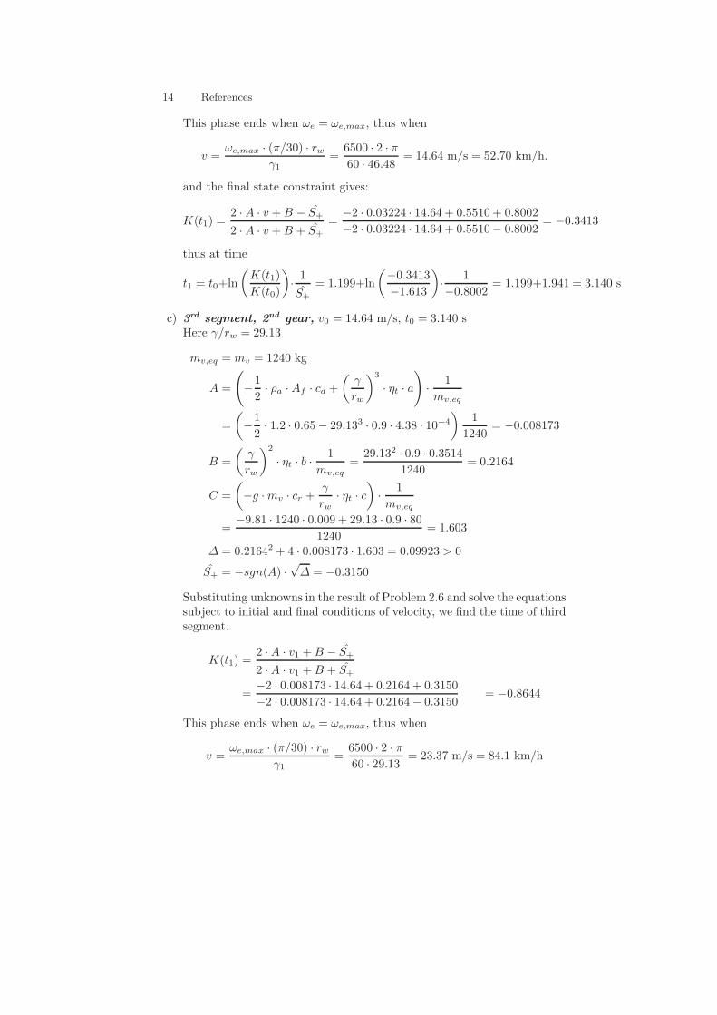
10 References
This phase ends when ωe = ωe,max, thus when
v =ωe,max · (π/30) · rw
γ1=
6500 · 2 · π60 · 46.48
= 14.64 m/s = 52.70 km/h.
and the final state constraint gives:
K(t1) =2 · A · v +B − S+
2 · A · v +B + S+
=−2 · 0.02635 · 14.64 + 0.4504 + 0.6541
−2 · 0.02635 · 14.64 + 0.4504− 0.6541= −0.3414
thus at time
t1 = t0+ln
(K(t1)
K(t0)
)·1
S+
= 1.467+ln
(−0.3414
−1.613
)·
1
−0.6541= 1.467+2.374 = 3.841 s
e) 3rd segment, 2nd gear, v0 = 14.64 m/s, t0 = 3.841 sHere γ/rw = 29.13
mv,eq = mv +Θe ·(γ
rw
)2
= 1240 + 0.128 · 29.132 = 1349 kg
A =
(
−1
2· ρa ·Af · cd +
(γ
rw
)3
· ηt · a
)
·1
mv,eq
=
(−1
2· 1.2 · 0.65− 29.133 · 0.9 · 4.38 · 10−4
)1
1349= −0.007512
B =
(γ
rw
)2
· ηt · b ·1
mv,eq=
29.132 · 0.9 · 0.35141349
= 0.1989
C =
(−g ·mv · cr +
γ
rw· ηt · c
)·
1
mv,eq
=−9.81 · 1240 · 0.009 + 29.13 · 0.9 · 80
1349= 1.474
∆ = 0.19892 + 4 · 0.007512 · 1.474 = 0.08385 > 0
S+ = −sgn(A) ·√∆ = −0.2896
Substituting unknowns in the result of Problem 2.6 and solve the equationssubject to initial and final conditions of velocity, we find the time of thirdsegment.
K(t1) =2 ·A · v1 +B − S+
2 ·A · v1 +B + S+
=−2 · 0.007512 · 14.64 + 0.1989 + 0.2896
−2 · 0.007512 · 14.64 + 0.1989− 0.2896= −0.8645
This phase ends when ωe = ωe,max, thus when
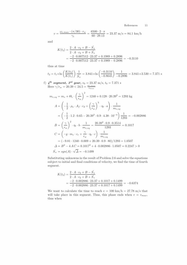
References 11
v =ωe,max · (π/30) · rw
γ1=
6500 · 2 · π60 · 29.13
= 23.37 m/s = 84.1 km/h
and
K(t2) =2 · A · v2 +B − S+
2 · A · v2 +B + S+
=−2 · 0.007512 · 23.37 + 0.1989 + 0.2896
−2 · 0.007512 · 23.37 + 0.1989− 0.2896= −0.3110
thus at time
t2 = t1+ln
(K(t2)
K(t1)
)·1
S+
= 3.841+ln
(−0.3110
−0.8645
)·
1
−0.2896= 3.841+3.530 = 7.371 s
f) 4th segment, 3rd gear, v0 = 23.37 m/s, t0 = 7.371 sHere γ/rw = 20.39 < 24.5 = ωe,max
vmax
mv,eq = mv +Θe ·(γ
rw
)2
= 1240 + 0.128 · 20.392 = 1293 kg
A =
(
−1
2· ρa ·Af · cd +
(γ
rw
)3
· ηt · a
)
·1
mv,eq
=
(−1
2· 1.2 · 0.65− 20.393 · 0.9 · 4.38 · 10−4
)1
1293= −0.002886
B =
(γ
rw
)2
· ηt · b ·1
mv,eq=
20.392 · 0.9 · 0.35141293
= 0.1017
C =
(−g ·mv · cr +
γ
rw· ηt · c
)·
1
mv,eq
= (−9.81 · 1240 · 0.009 + 20.39 · 0.9 · 80)/1293 = 1.0507
∆ = B2 − 4AC = 0.10172 + 4 · 0.002886 · 1.0507 = 0.2247 > 0
S+ = sgn(A) ·√∆ = −0.1499
Substituting unknowns in the result of Problem 2.6 and solve the equationssubject to initial and final conditions of velocity, we find the time of fourthsegment.
K(t2) =2 · A · v2 +B − S+
2 · A · v2 +B + S+
=−2 · 0.002886 · 23.37 + 0.1017 + 0.1499
−2 · 0.002886 · 23.37 + 0.1017 + 0.1499= −0.6374
We want to calculate the time to reach v = 100 km/h = 27.78 m/s thatwill take place in this segment. Thus, this phase ends when v = vmax,thus when
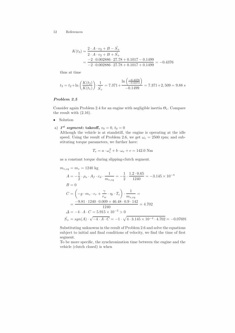
12 References
K(t3) =2 · A · v2 +B − S+
2 · A · v2 +B + S+
=−2 · 0.002886 · 27.78 + 0.1017− 0.1499
−2 · 0.002886 · 27.78 + 0.1017 + 0.1499= −0.4376
thus at time
t3 = t2+ln
(K(t2)
K(t1)
)·1
S+
= 7.371+ln(
−0.4376−0.6374
)
−0.1499= 7.371+2, 509 = 9.88 s
Problem 2.5
Consider again Problem 2.4 for an engine with negligible inertia Θe. Comparethe result with (2.16).
• Solution
a) 1st segment : takeoff, v0 = 0, t0 = 0Although the vehicle is at standstill, the engine is operating at the idlespeed. Using the result of Problem 2.6, we get ωe = 2500 rpm; and sub-stituting torque parameters, we further have:
Te = a · ω2e + b · ωe + c = 142.0 Nm
as a constant torque during slipping-clutch segment.
mv,eq = mv = 1240 kg
A = −1
2· ρa · Af · cd ·
1
mv,eq= −
1
2·1.2 · 0.651240
= −3.145× 10⁻⁴
B = 0
C =
(−g ·mv · cr +
γ
rw· ηt · Te
)·
1
mv,eq=
=−9.81 · 1240 · 0.009 + 46.48 · 0.9 · 142
1240= 4.702
∆ = −4 · A · C = 5.915× 10⁻³ > 0
S+ = sgn(A) ·√−4 ·A · C = −1 ·
√4 · 3.145× 10−4 · 4.702 = −0.07691
Substituting unknowns in the result of Problem 2.6 and solve the equationssubject to initial and final conditions of velocity, we find the time of firstsegment.To be more specific, the synchronization time between the engine and thevehicle (clutch closed) is when
References 13
v =ωe[rpm] · (π/30) · rw
γ= 5.633 m/s = 20.28 km/h,
thus the final state constraint of the first segment appears to be:
K(t0) =2 · A · v − S
2 · A · v + S=
2 · (−3.145) · 10−4 · 5.633 + 0.07691
2 · (−3.145) · 10−4 · 5.633− 0.07691= −0.9119
Because the evolution of K(t) satisfies K(t) = K0 ·eS+(t−t0)], the synchro-nize time is thus
S+ = sgn(A) ·√∆ = −0.07691, K0 = −1
t =ln(
K(t0)K0
)
S+
=ln(−0.9119
−1 )
−0.07691= 1.199 s
b) 2nd segment, 1st gear, v0 = 5.633 m/s, t0 = 1.199 s
Here γ/rw = 46.48, thus
mv,eq = mv = 1240 kg
A =
(
−1
2· ρa ·Af · cd +
(γ
rw
)3
· ηt · a
)
·1
mv,eq
=
(−1
2· 1.2 · 0.65− 46.483 · 0.9 · 4.38 · 10−4
)·
1
1240= −0.03224
B =
(γ
rw
)2
· ηt · b ·1
mv,eq=
46.482 · 0.9 · 0.35141240
= 0.5510
C =
(−g ·mv · cr +
γ
rw· ηt · c
)·
1
mv,eq
=−9.81 · 1240 · 0.009 + 46.48 · 0.9 · 80
1240= 2.611
∆ = B2 − 4 · A · C = 0.55102 + 4 · 0.03224 · 2.611 = 0.6403 > 0
S+ = sgn(A) ·√∆ = −0.8002
Substituting unknowns in the result of Problem 2.6 and solve the equationssubject to initial and final conditions of velocity, we find the time of secondsegment.
K(t0) =2 · A · v0 +B − S+
2 · A · v0 +B + S+
=−2 · 0.03224 · 5.633 + 0.5510 + 0.8002
−2 · 0.03224 · 5.633 + 0.5510− 0.8002= −1.613
14 References
This phase ends when ωe = ωe,max, thus when
v =ωe,max · (π/30) · rw
γ1=
6500 · 2 · π60 · 46.48
= 14.64 m/s = 52.70 km/h.
and the final state constraint gives:
K(t1) =2 · A · v +B − S+
2 · A · v +B + S+
=−2 · 0.03224 · 14.64 + 0.5510 + 0.8002
−2 · 0.03224 · 14.64 + 0.5510− 0.8002= −0.3413
thus at time
t1 = t0+ln
(K(t1)
K(t0)
)·1
S+
= 1.199+ln
(−0.3413
−1.613
)·
1
−0.8002= 1.199+1.941 = 3.140 s
c) 3rd segment, 2nd gear, v0 = 14.64 m/s, t0 = 3.140 sHere γ/rw = 29.13
mv,eq = mv = 1240 kg
A =
(
−1
2· ρa ·Af · cd +
(γ
rw
)3
· ηt · a
)
·1
mv,eq
=
(−1
2· 1.2 · 0.65− 29.133 · 0.9 · 4.38 · 10−4
)1
1240= −0.008173
B =
(γ
rw
)2
· ηt · b ·1
mv,eq=
29.132 · 0.9 · 0.35141240
= 0.2164
C =
(−g ·mv · cr +
γ
rw· ηt · c
)·
1
mv,eq
=−9.81 · 1240 · 0.009 + 29.13 · 0.9 · 80
1240= 1.603
∆ = 0.21642 + 4 · 0.008173 · 1.603 = 0.09923 > 0
S+ = −sgn(A) ·√∆ = −0.3150
Substituting unknowns in the result of Problem 2.6 and solve the equationssubject to initial and final conditions of velocity, we find the time of thirdsegment.
K(t1) =2 ·A · v1 +B − S+
2 ·A · v1 +B + S+
=−2 · 0.008173 · 14.64 + 0.2164 + 0.3150
−2 · 0.008173 · 14.64 + 0.2164− 0.3150= −0.8644
This phase ends when ωe = ωe,max, thus when
v =ωe,max · (π/30) · rw
γ1=
6500 · 2 · π60 · 29.13
= 23.37 m/s = 84.1 km/h
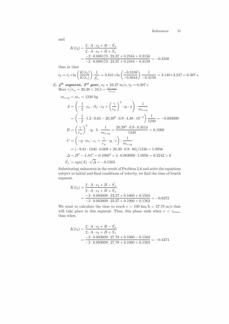
References 15
and
K(t2) =2 · A · v2 +B − S+
2 · A · v2 +B + S+
=−2 · 0.008173 · 23.37 + 0.2164 + 0.3150
−2 · 0.008173 · 23.37 + 0.2164− 0.3150= −0.3108
thus at time
t2 = t1+ln
(K(t2)
K(t1)
)·1
S+
= 3.841+ln
(−0.3108
−0.8644
)·
1
−0.3150= 3.140+3.247 = 6.387 s
d) 4th segment, 3rd gear, v0 = 23.37 m/s, t0 = 6.387 sHere γ/rw = 20.39 < 24.5 = ωe,max
vmax
mv,eq = mv = 1240 kg
A =
(
−1
2· ρa ·Af · cd +
(γ
rw
)3
· ηt · a
)
·1
mv,eq
=
(−1
2· 1.2 · 0.65− 20.393 · 0.9 · 4.38 · 10−4
)1
1240= −0.003009
B =
(γ
rw
)2
· ηt · b ·1
mv,eq=
20.392 · 0.9 · 0.35141240
= 0.1060
C =
(−g ·mv · cr +
γ
rw· ηt · c
)·
1
mv,eq
= (−9.81 · 1240 · 0.009 + 20.39 · 0.9 · 80)/1240 = 1.0956
∆ = B2 − 4AC = 0.10602 + 4 · 0.003009 · 1.0956 = 0.2242 > 0
S+ = sgn(A) ·√∆ = −0.1563
Substituting unknowns in the result of Problem 2.6 and solve the equationssubject to initial and final conditions of velocity, we find the time of fourthsegment.
K(t2) =2 · A · v2 +B − S+
2 · A · v2 +B + S+
=−2 · 0.003009 · 23.37 + 0.1060 + 0.1563
−2 · 0.003009 · 23.37 + 0.1060 + 0.1563= −0.6372
We want to calculate the time to reach v = 100 km/h = 27.78 m/s thatwill take place in this segment. Thus, this phase ends when v = vmax,thus when
K(t3) =2 · A · v2 +B − S+
2 · A · v2 +B + S+
=−2 · 0.003009 · 27.78 + 0.1060− 0.1563
−2 · 0.003009 · 27.78 + 0.1060 + 0.1563= −0.4374
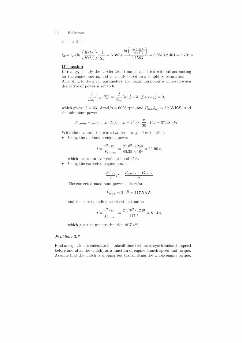
16 References
thus at time
t3 = t2+ln
(K(t2)
K(t1)
)·1
S+
= 6.387+ln(
−0.0.4374−0.6372
)
−0.1563= 6.387+2.404 = 8.791 s
DiscussionIn reality, usually the acceleration time is calculated without accountingfor the engine inertia, and is usually based on a simplified estimation.According to the given parameters, the maximum power is achieved whenderivative of power is set to 0:
d
dωe(ωe · Te) =
d
dωe(aω3
e + bω2e + cωe) = 0,
which gives ω∗e = 631.3 rad/s = 6028 rpm, and Pmax|ω∗
e= 80.35 kW. And
the minimum power:
Pe,min = ωe,launch · Te,launch = 2500 ·π
30· 142 = 37.18 kW
With these values, there are two basic ways of estimation:• Using the maximum engine power
t =v2 ·mv
Pe,max=
27.82 · 124080.35× 103
= 11.90 s,
which means an over-estimation of 35%.• Using the corrected engine power
˜Pmax
2P =
Pe,max + Pe,min
2
The corrected maximum power is therefore:
˜Pmax = 2 · P = 117.5 kW,
and the corresponding acceleration time is:
t =v2 ·mv
˜Pe,max
=27.782 · 1240
117.5= 8.14 s,
which gives an underestimation of 7.4%.
Problem 2.6
Find an equation to calculate the takeoff time (=time to synchronise the speedbefore and after the clutch) as a function of engine launch speed and torque.Assume that the clutch is slipping but transmitting the whole engine torque.
References 17
• Solution
Assume the ratio of gear-ratio to wheel diameter is kept at gear 1 duringthe take-off time; and the engine torque is kept constant while enginespeed ωe and wheel speed v are therefore decoupled.
a) Check Delta of the motionGiven the constant torque as input, the law of motion of the type v =A · v2 + C, where
A = −1
2· ρa ·Af · cd ·
1
mv,eqC =
(−g ·mv · cr +
γ
rw· ηt · Te
)·
1
mv,eq
Given the fact that A < 0, B = 0, we have ∆ = −4AC > 0, thenS+ = sgnA ·
√∆ = −
√∆.
b) Solve the motion law with final conditionGiven that t0 = 0, v0 = 0, then
K0 =2Av0 +B − S+
2Av0 +B + S+
= −1.
and the synchronized speed of the wheel should balance the idel speed ofthe engine:
vf = ωe,idle ·rwγ.
then
K(tf) =2Avf +B − S+
2Avf +B + S+
=2Avf − S+
2Avf + S+
.
Since K(tf ) = K0 · eS+(tf−t0), we have
tf =ln
2Avf−S+
2Avf+S+
−1
S+
Therefore,
ttakeoff =ln(−K)
S+
Problem 2.7
Evaluate the coasting speed and the roll-out time without acting on the brakesfor a vehicle with an initial speed v0 = 50 km/h and mv = 1200 kg, Af · cd =0.65m2, cr = 0.009. Assume the clutch open (no engine friction).
• Solution
18 References
Assume the coasting speed is defined when the engine is disengaged andthe resistence loss of the vehicle matches exactly the decrease of its kineticenergy:
d
dtvc(t) = −
1
2mv· ρaAf · Cd v
2c (t)− g Cr
and we let:
α2 =ρa · AfCd · v2c (t)
2mv= −A
β2 = g Cr = −C
a) Check Delta of the motionGiven the zero torque as input(engine disengaged), the law of motion ofthe type v = A · v2 + C, where
A = −1
2mv· ρaAf · Cd C = −g Cr
Given the fact that A < 0, B = 0, C < 0, we have ∆ = −4AC < 0,therefore we have equation (2.18).
b) Calculate coasting speedThe coasting speed as a function of time (2.18) is
v(t) =β
α· tan
arctan
(α
β· v0)− α · β · t
where
α =
√1
2·ρa · Af · cd
mv=
√1
2·1.2 · 0.651200
= 0.01803
β =√g · cr =
√9.81 · 0.009 = 0.2971
c) Calculate the roll-off timeThe braking time at which v = 0 is calculated by solving:
0 =β
αtan
[arctan
(α
βv0
)− αβ · t
]
trollout =1
α · β· arctan
(α
β· v0)
=1
0.018 · 0.297· arctan
(0.018
0.297·50
3.6
)= 130.75 s
DiscussionTake care of the radians calculation in the function arctan.
References 19
Mechanical Energy Demand in Driving Cycles
Problem 2.8
Evaluate the traction energy and the recuperation energy for the MVEG–95for the vehicle examples of Fig. 2.8, left and right, assuming perfect recuper-ation.
• Solution
Assume the time intervals in traction mode are not subject ot change dur-ing artificial cycles like MVEG-95, so the equations used in this problemis only valid if this assumption holds; and the track length of MVEG-95is 0.114 km.
a) Left graph configuration (Af · Cd = 0.7 m2,mv = 1500 kg, Cr = 0.012)
(i) The traction energy is given by (2.31), assuming no recuperation.
E = Ediss + Ecirc = [1.9× 10⁴ ·AfCd + 8.4× 10² ·mv Cr + 10 ·mv] · xtot
=(0.7 · 1.9 · 104 + 1500 · 0.012 · 8.4 · 102 + 1500 · 10
)
= 43.42 MJ/100 km · xtot = 43.42 · 0.114 = 4.950 MJ.
(ii) The total energy is given by (2.35), assuming perfect recuperation.
Erec = Ediss = [2.2× 10⁴ · AfCd + 9.8× 10² ·mv Cr] · xtot
=(0.7 · 2.2 · 104 + 1500 · 0.012 · 9.81 · 102
)=
= 33.04 MJ/100 km · xtot = 3.767 MJ.
(iii) The energy that can be recuperated:
∆E = E − Erec = 1.183 MJ (24.75% of )E.
b) Right graph configuration (Af · Cd = 0.4 m2,mv = 750 kg, Cr = 0.008)
(i) The traction energy is given by (2.31), assuming no recuperation.
E = Ediss + Ecirc = [1.9× 10⁴ ·AfCd + 8.4× 10² ·mv Cr + 10 ·mv] · xtot
=(0.4 · 1.9 · 104 + 1500 · 0.008 · 8.4 · 102 + 750 · 10
)
= 20.14 MJ/100 km · xtot = 20.14 · 0.114 = 2.296 MJ.
(ii) The total energy is given by (2.35), assuming perfect recuperation.
Erec = Ediss = [2.2× 10⁴ · AfCd + 9.8× 10² ·mv Cr] · xtot
=(0.4 · 2.2 · 104 + 750 · 0.008 · 9.81 · 102
)=
= 14.68 MJ/100 km · xtot = 1.674 MJ.
(iii) The energy that can be recuperated:
∆E = E − Erec = 0.622 MJ (27.09% of )E.
The potential of regenerative braking is more important for the smaller vehi-cle, with smaller front area, vehicle mass and rolling friction coefficient.
20 References
Problem 2.9
Calculate the mean force and fuel consumption data shown in Fig. 2.8 left.
• Solution
Assume left graph configuration (Af · Cd = 0.7 m2,mv = 1500 kg, Cr =0.012)
a) Case 1: No recuperationReading constants from (2.30), we get the weights during traction modesof the cycle MVEG-95:
Ftrac,a =1
2· ρa · Af · cd · 319 =
1
2· 1.2 · 0.7 · 319 = 134.0 N
Ftrac,r = mv · g · cr · 0.856 = 1500 · 9.81 · 0.012 · 0.856 = 151.2 N
Ftrac,m = mv · 0.101 = 1500 · 0.101 = 151.5 N
The mechanical energy per 100 km that corresponds to 1N is
dmf = 1 N · 105 m = 105 J = 105/3600 = 27.78 Wh.
And according to the caption of Figure 2.8, Diesel’s LHV is 104W h/l,which gives:
1 N = 27.78 Wh/100km = 2.778× 10⁻³ l/100km
Therefore, for no-recuperation,
∗V= ¯Ftrac × dmf = 436.6× 2.778× 10−3 = 1.213 l/100km
b) Case 2: Perfect recuperationReading constants from (2.34), we get the weights for perfect recupera-tion over the cycle MVEG-95:
Fa =1
2· ρa ·Af · cd · 363 =
1
2· 1.2 · 0.7 · 363 = 152.5 N
Fr = mv · g · cr · 1 = 1500 · 9.81 · 0.012 · 1 = 176.6 N
Therefore, for perfect-recuperation,
∗V= F × dmf = 329.1× 2.778× 10−3 = 0.9142 l/100km
Discussion(i) Evaluation of the differences in mean force
Fm,r = 152.5 + 176.6− (134.0 + 151.2) = 43.9 N
Fm,b = 436.6− 329.1 = 107.5 N
References 21
where Fm,r denotes the mean force that is used to overcome the drivingresistance in the non-traction phases; while Fm,b denotes the part ofmean force that is later dissipated by heat with the brakes.
(ii) Explanatory comments on calculating mean force with/without recu-peration
• When no recuperation is done, Ftrac overcomes aerodynamic drag,rolling friction drag and acceleration requirement when ‘trac”mode is on; while during coasting, non of them is of the concern ofenergy consumption, since the kinetic energy at high vehicle speedapparently cost more energy and cannot be recuperated
• When perfect recuperation is done, Ftrac overcomes aerodynamicdrag, rolling friction drag and acceleration requirement all throughthe cycle. Especially during coasting, braking or not braking is stillof the energy concern since the kinetic energy at high speed canbe later recuperated, if the speed profile can be satisfied with thehelp of “recuperative brake”. If it is not the case, mechanical brakehas to intervene, so as to dissipate the remaining part of energyand satisfy speed profile.
Problem 2.10
Calculate the data in Fig. 2.9, left and right.
• Solution
a) Full-sized vehicle ((Af · Cd = 0.7 m2,mv = 1500 kg, Cr = 0.012))The cycle energy assuming no recuperation is given by (2.31),
E = [1.9× 10⁴ · AfCd + 8.4× 10² ·mv Cr + 10 ·mv] · xtot
= 0.7 · 1.9 · 104 + 1500 · 0.012 · 8.4 · 102 + 1500 · 10= 43 · 103 kJ/100 km,
thus
22 References
S(Af · cd) =∂E
∂(Af · Cd)·
Af · Cd
E(Af · Cd)
=1.9 · 104 · 0.7
43 · 103= 0.3046
S(cr) =∂E
∂(Cr)·
Cr
E(Cr)
=1500 · 8.4 · 102 · 0.012
43 · 103= 0.3463
S(mv) =∂E
∂(mv)·
mv
E(mv)
=(0.012 · 8.4 · 102 + 10) · 1500
43 · 103= 0.6899
b) Light-weight vehicle ((Af · Cd = 0.4 m2,mv = 750 kg, Cr = 0.008))
E = [1.9× 10⁴ · AfCd + 8.4× 10² ·mv Cr + 10 ·mv] · xtot
= 0.4 · 1.9 · 104 + 750 · 0.008 · 8.4 · 102 + 750 · 10= 20 · 103 kJ/100 km
thus
S(Af · cd) =∂E
∂(Af · Cd)·
Af · Cd
E(Af · Cd)
=1.9 · 104 · 0.4
20 · 103= 0.3774
S(cr) =∂E
∂(Cr)·
Cr
E(Cr)
=750 · 8.4 · 102 · 0.008
20 · 103= 0.2502
S(mv) =∂E
∂(mv)·
mv
E(mv)
=(0.008 · 8.4 · 102 + 10) · 750
20 · 103= 0.6226
DiscussionFrom the result we can conclude, with an advanced vehicle concept (usu-ally light-weight and smaller rolling friction):• relative dominance of the vehicle mass on the energy consumption is
unchanged around a level of 60% to 70%, which makes kinetic energyrecuperation an interesting choice.
• Relative influence of the rolling fricition becomes less than that ofAf · Cd (coefficient of aerodynamic force.)
References 23
Problem 2.11
Calculate which constant vehicle speed on a flat road is responsible for thesame energy demand at the wheels along a MVEG–95 cycle, in the case ofno recuperation and of perfect recuperation, respectively. Assume the light-weight vehicle data of Fig. 2.8, right side of Figure: Af · cd,mv, cr =0.4 m2, 750 kg, 0.008.• Solution
a) No recuperationThe cycle energy is calculated in Problem 2.8 and it is E = 20.14 ·103 kJ/100 km. The mean traction force is
F =E
100 km= 201.4 N
To have the same F , find v such that
1
2· ρa ·Af · cd · v2 +mv · g · cr = F
v =
√
2 ·Ftrac −mv · g · cr
ρa · Af · cd
v =
√2 ·
201.4− 750 · 9.81 · 0.0081.2 · 0.4
= 24.35 m/s = 87.67 km/h
b) Perfect recuperationHere, E = 14.68 · 103 kJ/100 km, thus
F = 146.8 N
v = 19.5 m/s = 70 km/h
To have the same F , find v such that
1
2· ρa ·Af · cd · v2 +mv · g · cr = F
v =
√
2 ·Ftrac −mv · g · cr
ρa ·Af · cd
v =
√2 ·
146.8− 750 · 9.81 · 0.0081.2 · 0.4
= 19.14 m/s = 68.9 km/h
Discussion
• Note that the mechanical mean force is not accounted for, because theproblem assumes instantaneous energy consumption during flat roadconstant speed cruising.
• Note that for artificial driving cycles like MVEG-95, the equivalentspeed can also be calculated by equating mean force representationwith (2.31) or (2.35), respectively.
24 References
Problem 2.12
Calculate the maximum mass allowed for a recuperation system with ηrec =40%. Use the vehicle parameters of Fig. 2.12: Af ·cd,mv, cr = 0.7 m2, 1500 kg, 0.012.
• Solution
a) Deriving the energy demand with a real recuperation deviceUsing the equations (2.31),(2.35),(2.39),(2.40):
Ediss + Ecirc = [1.9× 10⁴ · AfCd + 8.4× 10² ·mv Cr + 10 ·mv]
Ediss = [2.2× 10⁴ · AfCd + 9.8× 10² ·mv Cr]
E(ηrec,mrec) = ¯Ediss(mrec) + (1− ηrec)Ecirc(mrec)¯Ecirc = E − ¯Ediss
we get:
¯E(ηrec,mrec)
= [22000− 3000(1− ηrec)]Af · Cd + [980− 140(1− ηrec)]Cr (mv +mrec + 10 (1− ηrec) · (mv +mrec
= (22000− 3000)× 0.6× 0.7 + [980− 140× 0.6]× 0.012 (1500+mrec) + 10× 0.6 (1500+mrec)
c) Equate the energy demand and get the maximum mass of recuperationdeviceWhen we have the maximum weight of recuperation device, the meanenergy demand must equal E, which has been calculated in Problem 2.8as 43.4 · 103 kJ/100 km. Thus
mv =(43.4− 14.1) · 103
16.75= 1750 kg
14140 + 16.752× (1500 +mrec) = 43.66× 10³
mrec = 262.2 kg.
The maximum weight is the one that leads to an energy demand equal to theenergy demand without recuperation. Thus, from (2.41)
E(ηrec,mrec) = 0.7 · (2.2 · 104 − 0.6 · 3 · 103)++ 0.012 · mv · (9.8 · 102 − 0.6 · 1.4 · 102)++ 0.6 · 10 · mv =
= 14.1 · 103 + (10.75 + 6) · mv (kJ/100 km)
where mv = mv +mrec.
References 25
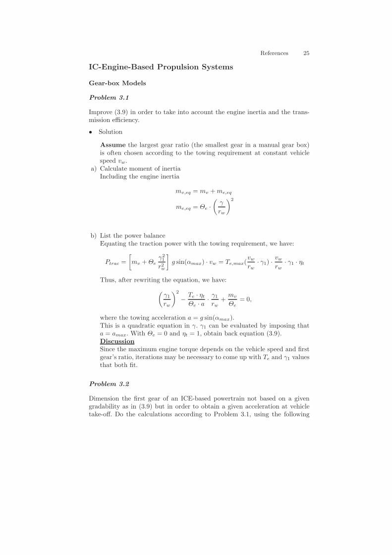
IC-Engine-Based Propulsion Systems
Gear-box Models
Problem 3.1
Improve (3.9) in order to take into account the engine inertia and the trans-mission efficiency.
• Solution
Assume the largest gear ratio (the smallest gear in a manual gear box)is often chosen according to the towing requirement at constant vehiclespeed vw.
a) Calculate moment of inertiaIncluding the engine inertia
mv,eq = mv +me,eq
me,eq = Θe ·(γ
rw
)2
b) List the power balanceEquating the traction power with the towing requirement, we have:
Ptrac =
[mv +Θe
γ21r2w
]g sin(αmax) · vw = Te,max(
vwrw
· γ1) ·vwrw
· γ1 · ηt
Thus, after rewriting the equation, we have:
(γ1rw
)2
−Te · ηtΘe · a
·γ1rw
+mv
Θe= 0,
where the towing acceleration a = g sin(αmax).This is a quadratic equation in γ. γ1 can be evaluated by imposing thata = amax. With Θe = 0 and ηt = 1, obtain back equation (3.9).DiscussionSince the maximum engine torque depends on the vehicle speed and firstgear’s ratio, iterations may be necessary to come up with Te and γ1 valuesthat both fit.
Problem 3.2
Dimension the first gear of an ICE-based powertrain not based on a givengradability as in (3.9) but in order to obtain a given acceleration at vehicletake-off. Do the calculations according to Problem 3.1, using the following
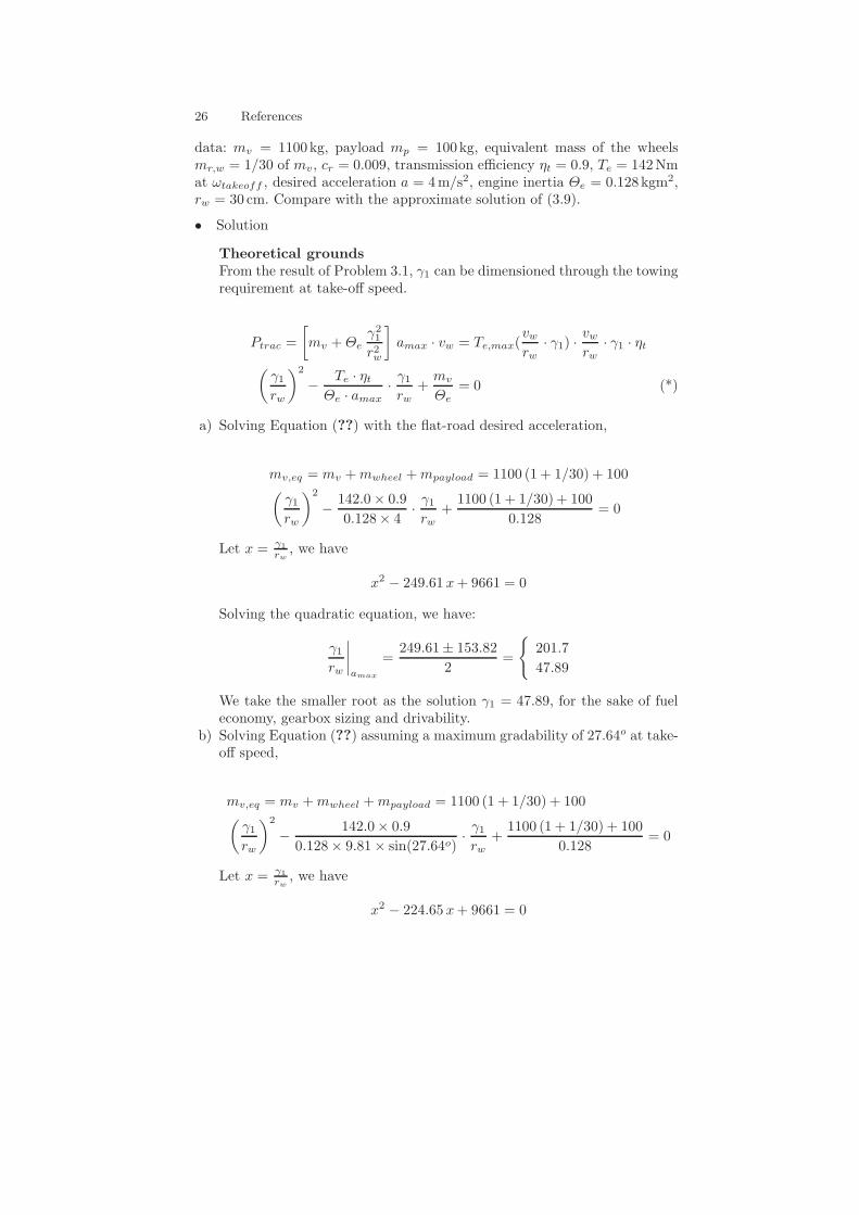
26 References
data: mv = 1100kg, payload mp = 100kg, equivalent mass of the wheelsmr,w = 1/30 of mv, cr = 0.009, transmission efficiency ηt = 0.9, Te = 142Nmat ωtakeoff , desired acceleration a = 4m/s2, engine inertia Θe = 0.128kgm2,rw = 30 cm. Compare with the approximate solution of (3.9).
• Solution
Theoretical groundsFrom the result of Problem 3.1, γ1 can be dimensioned through the towingrequirement at take-off speed.
Ptrac =
[mv +Θe
γ21r2w
]amax · vw = Te,max(
vwrw
· γ1) ·vwrw
· γ1 · ηt(γ1rw
)2
−Te · ηt
Θe · amax·γ1rw
+mv
Θe= 0 (*)
a) Solving Equation (??) with the flat-road desired acceleration,
mv,eq = mv +mwheel +mpayload = 1100 (1 + 1/30) + 100(γ1rw
)2
−142.0× 0.9
0.128× 4·γ1rw
+1100 (1 + 1/30) + 100
0.128= 0
Let x = γ1
rw, we have
x2 − 249.61 x+ 9661 = 0
Solving the quadratic equation, we have:
γ1rw
∣∣∣∣amax
=249.61± 153.82
2=
201.7
47.89
We take the smaller root as the solution γ1 = 47.89, for the sake of fueleconomy, gearbox sizing and drivability.
b) Solving Equation (??) assuming a maximum gradability of 27.64o at take-off speed,
mv,eq = mv +mwheel +mpayload = 1100 (1 + 1/30) + 100(γ1rw
)2
−142.0× 0.9
0.128× 9.81× sin(27.64o)·γ1rw
+1100 (1 + 1/30) + 100
0.128= 0
Let x = γ1
rw, we have
x2 − 224.65 x+ 9661 = 0
References 27
Solving the quadratic equation, we have:
γ1rw
∣∣∣∣amax
=224.65± 108.74
2=
166.7
57.96
We take the smaller root as the solution γ1 = 57.96, for the sake of fueleconomy, gearbox sizing and drivability.
c) Calculate the approximate solutions with Equation (3.9)Accroding to (3.9), we have:
γ1 =mv rw · amax
Te,max(ωe),
where amax denotes the desired acceleration or gradability g · sin(αmax).Therefore, the approximated solutions are:
γ1,accr =[1100 (1 + 1/30) + 100]× 0.30× 4
142.0= 34.83,
for desired acceleration of 4 m/s2
γ1,grad =[1100 (1 + 1/30) + 100]× 0.30× 9.81× sin(27.64o)
142.0= 38.71,
for desired gradability of 27.64o
d) Comparison of Problem 3.2 with approximated equation (3.9)The results of the four cases are listed in the table: From the results, we
Table 10.2. Comparison of first gear with different ways of calculation.
Results γ1rw
γ1|rw=0.3m
Exact with aflat 47.89 14.367
Approx with aflat 34.83 10.449
Exact with αgrad 57.96 17.388
Approx with αgrad 38.71 11.613
could conclude that• Including more types of losses (e.g. rotational moment of inertia/
transmission efficiency) would increase the gear ratio γ1.• Increasing the requirement of gradability or acceleration capability
would decrease the 1st order term of the quadratic equation (??), whichindirectly increases the gear ratio γ1.
DiscussionThe multiple roots of quadratic equation adds to complexity of the firstgear dimensionization. However, usually only the smaller positive rootmakes sense for the following reasons:
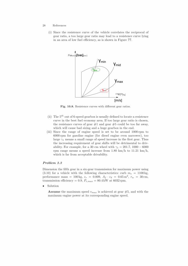
28 References
(i) Since the resistence curve of the vehicle correlates the reciprocal ofgear ratio, a too large gear ratio may lead to a resistence curve lyingin an area of low fuel efficiency, as is shown in Figure ??.
ηmax
ηmin
γmidγmin
γmax
[bar]
[m/s]
pwt
mf [kg]curve
(motor + engine)
Fig. 10.8. Resistence curves with different gear ratios.
(ii) The 5th out of 6-speed gearbox is usually defined to locate a resistencecurve in the best fuel economy area. If too large gear ratio is chosen,the resistance curves of gear #1 and gear #5 could be too far away,which will cause bad sizing and a huge gearbox in the end.
(iii) Since the range of engine speed is set to be around 1000 rpm to6000 rpm for gasoline engine (for diesel engine even narrower), toolarge γ1 means a small range of speed increase in the first gear. Thusthe increasing requirement of gear shifts will be detrimental to driv-ability. For example, for a 30 cm wheel with γ1 = 201.7, 1000− 6000rpm range means a speed increase from 1.80 km/h to 11.21 km/h,which is far from acceptable drivability.
Problem 3.3
Dimension the fifth gear in a six-gear transmission for maximum power using(3.10) for a vehicle with the following characteristics: curb mv = 1100kg,performance mass = 100 kg, cr = 0.009, Af · cd = 0.65m2, rw = 30cm,transmission efficiency = 0.9, Pe,max = 80.4kW at 6032 rpm.
• Solution
Assume the maximum speed vmax is achieved at gear #5, and with themaximum engine power at its corresponding engine speed.
References 29
a) Maximum traction power at wheelHaving the engine power and transmission efficiency, we have:
Ptrac,max = Pe,max · ηt = 72.36 kW.
b) Solving equation (3.10), and find maximum speed:
Ptrac,max = Fmax · vmax
= vmax ·[mv g Cr vmax +
1
2ρa AfCd v
2max
]∣∣∣∣gear=5
.
By solving the equation
−72.36× 10³ + 105.95 vmax + 0.39 vmax3 = 0,
we have the only solution of real number
vmax|gear=5 = 55.45 m/s = 199.6 km/h
c) Calculate the gear ratioWith the maximum speed achieved with maximum engine power,
γ5rw
=π
30×ωe|Pmax
vmax
=π
30·6032
55.45= 11.392
γ5 = 3.418.
where a common wheel radius of 30 cm is used for calculation.
Problem 3.4
Consider again the system of Problems 3.2–3.3. Calculate the vehicle speedvalues, vj at which the engine is at its maximum speed, for all the gears j.
• Solution
Assume only the 2nd to 4th gear can be chosen according to a fixed law,while the 1st,5th and 6th are chosen with towing requirement, maximumpower and fuel efficiency, respectively.
a) Using geometric law
(i) Calculate the common ratio
1
κ= R1/4 = [
47.9
11.4]14 = 1.432,
γ1γ2
=γ2γ3
=γ3γ4
=γ4γ5
=1
κ= 1.432,
30 References
(ii) Find corresponding gear ratios
γ2rw
=γ1rw
· κ =47.89
1.432= 33.443,
γ3rw
=γ2rw
· κ =47.89
1.4322= 23.354,
γ4rw
=γ3rw
· κ =47.89
1.4323= 16.309,
γ5rw
= 11.392 (fixed and confirmed).
b) Using arithmetic law
(i) Calculate the common difference
R =1
k·(rwγi
−rwγi−k
)
=
(1
11.392−
1
47.89
)·1
4= 0.0167.
(ii) Find corresponding gear ratios
γ2rw
=1
rwγ1
+R=
11
47.89 + 0.0167= 26.609,
γ3rw
=1
rwγ2
+R=
11
26.609 + 0.0167= 18.422,
γ4rw
=1
rwγ3
+R=
11
18.422 + 0.0167= 14.088,
γ5rw
= 11.392 (fixed and confirmed).
c) Validate the shifting speedsThe shifting speeds denotes the vehicle speeds at the maximum enginespeed ωe,gs = 6032 rpm.
vk =π · ωe,gs
30 · γk
rw
,
thus the values in the following table.
Problem 3.5
Calculate the approximate efficiency of a clutch during a vehicle takeoff ma-neuver.
References 31
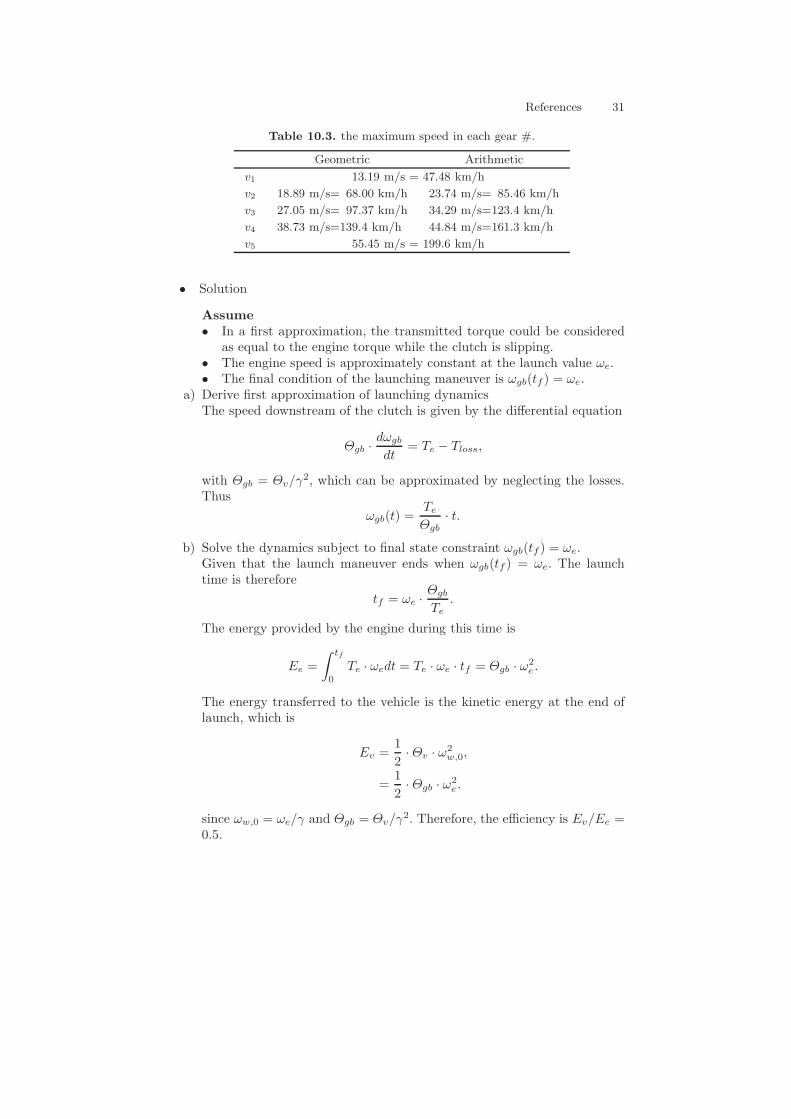
Table 10.3. the maximum speed in each gear #.
Geometric Arithmetic
v1 13.19 m/s = 47.48 km/h
v2 18.89 m/s= 68.00 km/h 23.74 m/s= 85.46 km/h
v3 27.05 m/s= 97.37 km/h 34.29 m/s=123.4 km/h
v4 38.73 m/s=139.4 km/h 44.84 m/s=161.3 km/h
v5 55.45 m/s = 199.6 km/h
• Solution
Assume• In a first approximation, the transmitted torque could be considered
as equal to the engine torque while the clutch is slipping.• The engine speed is approximately constant at the launch value ωe.• The final condition of the launching maneuver is ωgb(tf ) = ωe.
a) Derive first approximation of launching dynamicsThe speed downstream of the clutch is given by the differential equation
Θgb ·dωgb
dt= Te − Tloss,
with Θgb = Θv/γ2, which can be approximated by neglecting the losses.Thus
ωgb(t) =Te
Θgb· t.
b) Solve the dynamics subject to final state constraint ωgb(tf ) = ωe.Given that the launch maneuver ends when ωgb(tf ) = ωe. The launchtime is therefore
tf = ωe ·Θgb
Te.
The energy provided by the engine during this time is
Ee =
∫ tf
0Te · ωedt = Te · ωe · tf = Θgb · ω2
e .
The energy transferred to the vehicle is the kinetic energy at the end oflaunch, which is
Ev =1
2· Θv · ω2
w,0,
=1
2· Θgb · ω2
e .
since ωw,0 = ωe/γ and Θgb = Θv/γ2. Therefore, the efficiency is Ev/Ee =0.5.
32 References
DiscussionThe corresponding synchronization speed is
v =ωeγrw
.
Thus the energy lost is Ee−Ev = 12 ·Θgb ·ω2
e which coincides with (3.16),
Ec =1
2· Θv · ω2
w,0.
Fuel Consumption of IC Engine Powertrains
Problem 3.6
Find the CO2 emission factor (g/km) as a function of the fuel consumptionrate (l/100km) for gasoline and diesel fuels. Use these average fuels (gaso-line, diesel) data: density ρ = 0.745, 0.832kg/l, carbon dioxide to fuel massfraction m = 3.17, 3.16.
• Solution
Assume
Consider the stoichiometric fuel burning reaction, with a fuel of the molarcomposition CHa:
CHa +(1 +
a
4
)O2 ! CO2 +
(a2
)H2O
a) Find the factor a from CO2 to mass fractionThe mol CO2/mol emission factor is 1. The kg CO2/kg emission factor isthus
m =MCO2
Mfuel=
12 + 2 · 1612 + a
=44
12 + a
Table 10.4. Factor a of Diesel and Gasoline.
Variables Gasoline Diesel
m 3.17 3.16
a 1.880 1.924
b) Mass of CO2 per litre of fuelThe kg/l factor is m · ρ, where ρ (kg/l) is the fuel density.where the fuel consumption of some engine is mf = C l/100km,
References 33
Table 10.5. CO2 emission factor of Diesel and Gasoline.
Variables Gasoline Diesel
m · ρ [gCO2/l] 2.362 2.629
CO2factor [gCO2/km] 23.62· C 26.29· C
Problem 3.7
Calculate the fuel consumption and the CO2 emission rate for the MVEG–95cycle for a vehicle having the following characteristics: mv = 1100kg, payload= 100kg, cd · Af = 0.7, cr = 0.013, egb = 0.98, P0,gb = 3%, Paux = 250W,vlaunch = 3m/s, e = 0.4, Pe,0 = 1.26 kW, Pe,max = 66kW, diesel fuel (Hf =
43.1MJ/kg, ρf = 832 g/l), idle consumption∗V f,idle= 150g/h. The declared
CO2 emission rate for this car is 99 g/km.
• Solution
Assume the parameters of the driving cycle MVEG-95:
• Launch event happens every 105 s.• Idling time is around 300 s.• The track length of the cycle is 11.4 km.• The fraction of time during traction mode is trac = 0.6.
a) Calculate mean force:Assuming no recuperation, negligible engine inertia, the mean force ofcycle MVEG-95 can be calculated as follows:
F = Ftrac,r + Ftrac,a + Ftrac,m
=1
xtot
∑
trac
mv g Cr vi · h+∑
trac
1
2ρaAfCd vi
3 · h+∑
trac
mvai · vi · h
= 1200× 9.81× 0.013× 0.856 +1
2× 1.2× 0.7× 319 + 1200× 0.101
= 386.2 N = 38.62× 10³ kJ/100km
b) Traction power considering different loadsJust like the calculation from (3.23) to (3.32), we further assume• launch event happens every 105 s, this part of energy is accounted for
with average power.• during the calculation of engine load, only traction mode is considered,
and thus the power need to be compensated with a coefficienct of 1trac
First, we calculate the equivalent engine power considering the tractionmode and transmission loss:
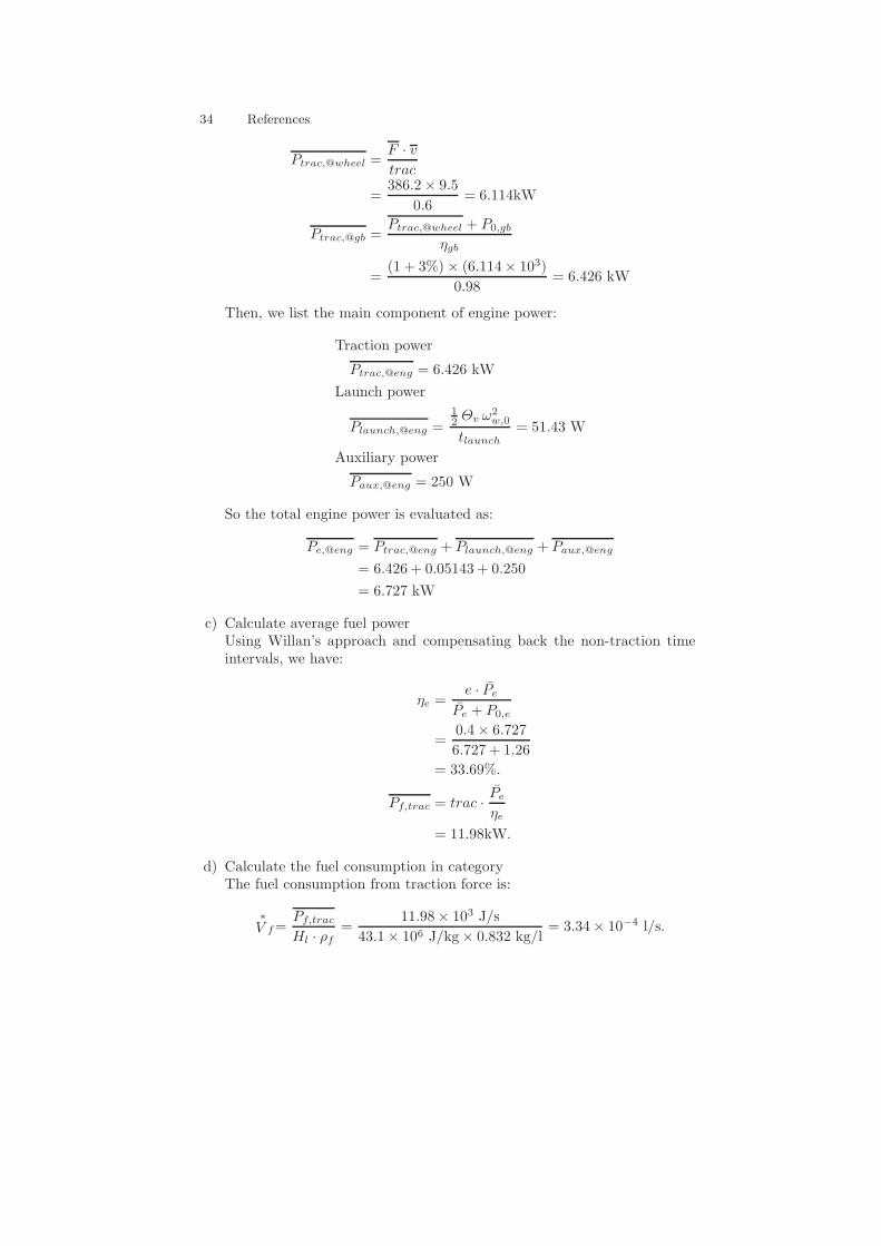
34 References
Ptrac,@wheel =F · vtrac
=386.2× 9.5
0.6= 6.114kW
Ptrac,@gb =Ptrac,@wheel + P0,gb
ηgb
=(1 + 3%)× (6.114× 10³)
0.98= 6.426 kW
Then, we list the main component of engine power:
Traction power
Ptrac,@eng = 6.426 kW
Launch power
Plaunch,@eng =12 Θv ω2
w,0
tlaunch= 51.43 W
Auxiliary power
Paux,@eng = 250 W
So the total engine power is evaluated as:
Pe,@eng = Ptrac,@eng + Plaunch,@eng + Paux,@eng
= 6.426 + 0.05143 + 0.250
= 6.727 kW
c) Calculate average fuel powerUsing Willan’s approach and compensating back the non-traction timeintervals, we have:
ηe =e · Pe
Pe + P0,e
=0.4× 6.727
6.727 + 1.26= 33.69%.
Pf,trac = trac ·Pe
ηe= 11.98kW.
d) Calculate the fuel consumption in categoryThe fuel consumption from traction force is:
∗V f=
Pf,trac
Hl · ρf=
11.98× 10³ J/s
43.1× 10⁶ J/kg× 0.832 kg/l= 3.34× 10⁻⁴ l/s.
References 35
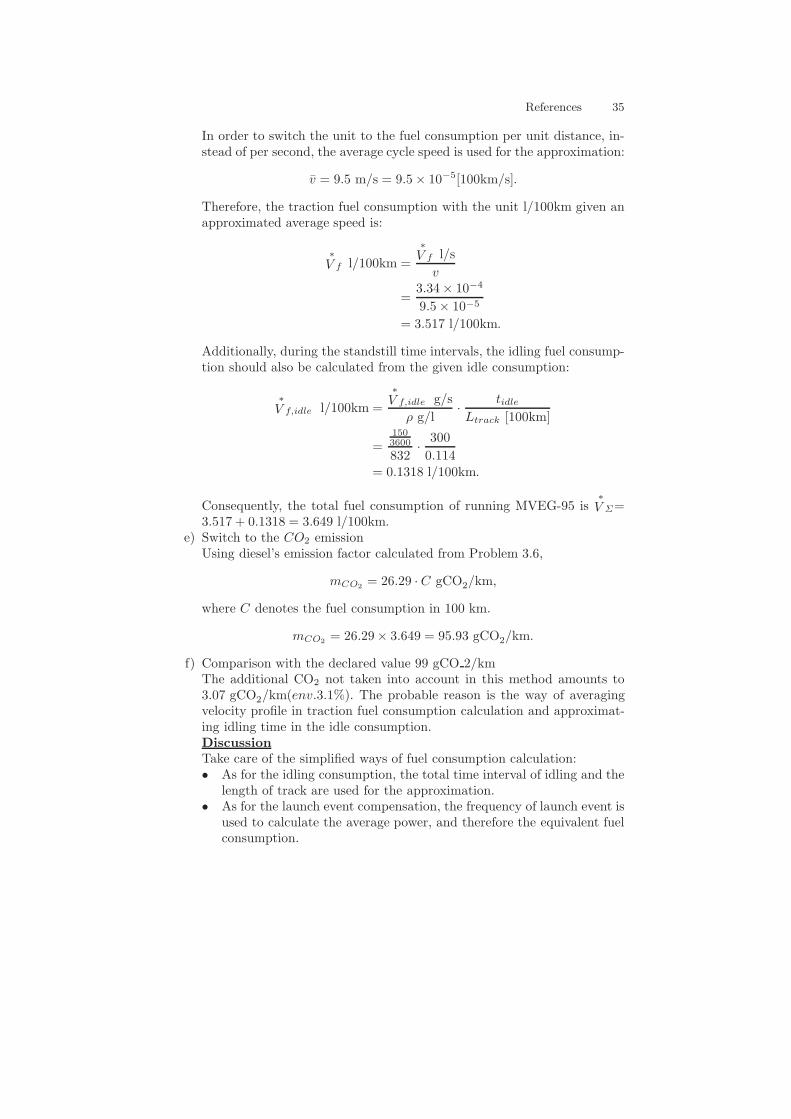
In order to switch the unit to the fuel consumption per unit distance, in-stead of per second, the average cycle speed is used for the approximation:
v = 9.5 m/s = 9.5× 10⁻⁵[100km/s].
Therefore, the traction fuel consumption with the unit l/100km given anapproximated average speed is:
∗V f l/100km =
∗V f l/s
v
=3.34× 10⁻⁴
9.5× 10−5
= 3.517 l/100km.
Additionally, during the standstill time intervals, the idling fuel consump-tion should also be calculated from the given idle consumption:
∗V f,idle l/100km =
∗V f,idle g/s
ρ g/l·
tidleLtrack [100km]
=1503600
832·300
0.114= 0.1318 l/100km.
Consequently, the total fuel consumption of running MVEG-95 is∗V Σ=
3.517 + 0.1318 = 3.649 l/100km.e) Switch to the CO2 emission
Using diesel’s emission factor calculated from Problem 3.6,
mCO2 = 26.29 · C gCO2/km,
where C denotes the fuel consumption in 100 km.
mCO2 = 26.29× 3.649 = 95.93 gCO2/km.
f) Comparison with the declared value 99 gCO 2/kmThe additional CO2 not taken into account in this method amounts to3.07 gCO2/km(env.3.1%). The probable reason is the way of averagingvelocity profile in traction fuel consumption calculation and approximat-ing idling time in the idle consumption.DiscussionTake care of the simplified ways of fuel consumption calculation:• As for the idling consumption, the total time interval of idling and the
length of track are used for the approximation.• As for the launch event compensation, the frequency of launch event is
used to calculate the average power, and therefore the equivalent fuelconsumption.
36 References
• As for the traction fuel consumption, the average cycle cpeed and thelength of track are used to switch the unit from fuel power to distance-specifc fuel consumption.
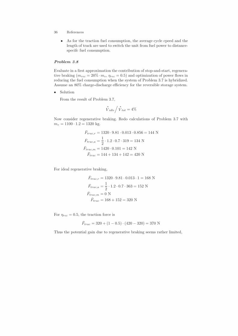
Problem 3.8
Evaluate in a first approximation the contribution of stop-and-start, regenera-tive braking (mrec = 20% ·mv, ηrec = 0.5) and optimization of power flows inreducing the fuel consumption when the system of Problem 3.7 is hybridized.Assume an 80% charge-discharge efficiency for the reversible storage system.
• Solution
From the result of Problem 3.7,
∗V idle
/ ∗V tot = 4%
Now consider regenerative braking. Redo calculations of Problem 3.7 withmv = 1100 · 1.2 = 1320 kg.
Ftrac,r = 1320 · 9.81 · 0.013 · 0.856 = 144 N
Ftrac,a =1
2· 1.2 · 0.7 · 319 = 134 N
Ftrac,m = 1420 · 0.101 = 142 N
Ftrac = 144 + 134 + 142 = 420 N
For ideal regenerative braking,
Ftrac,r = 1320 · 9.81 · 0.013 · 1 = 168 N
Ftrac,a =1
2· 1.2 · 0.7 · 363 = 152 N
Ftrac,m = 0 N
Ftrac = 168 + 152 = 320 N
For ηrec = 0.5, the traction force is
Ftrac = 320 + (1− 0.5) · (420− 320) = 370 N
Thus the potential gain due to regenerative braking seems rather limited,
References 37
Ptrac =370 · 9.5
0.6= 5.8 kW
P1 =5.8 · 103 · 1.03
0.98= 6.1 kW
Pstart =1
2·1200 · 32
105= 51 kW
Pe = 6.1 · 103 + 0.25 + 0.05 = 6.4 kW
ηe =e · Pe
Pe + P0,e=
0.4 · 6.46.4 + 1.26
= 0.33
Pf =0.6 · Pe
ηe= 11.6 kW
∗V trac =
11.6 · 103
43.1 · 106 · 0.832= 3.2 · 10−4 l/s =
=3.2 · 10−4
9.5· 105 l/100 km = 3.4 l/100 km
In summary we have 3.6 l/100 km w.r.t. 3.4 l/100 km. The benefit due to regen-erative braking is equal to the benefit due to idle consumption suppressionand they amount to 3%. To evaluate the potential benefit of engine oper-ating point shifting, assume that the engine could be able to work alwaysat its maximum efficiency point, thus at Pe,max = 66 kW. The efficiency isηe = 0.4 · 66/(66 + 1.26) = 0.39. Moreover, during a time t1, the engine de-livers its surplus power to the battery, to be reused later. An energy balanceacross the traction phase yields Pe · 0.6 = Pe,max · t1 +(Pe,max − Pe) · t1 · ηacc,where ηacc is the efficiency of the accumulation system (to be charged andthen discharged). Assuming ηacc = 0.8, from the latter one calculates
t1 =6.4 · 0.6
66 + (66− 6.4) · 0.8= 0.034,
thus
Pf =0.034 · 66 · 103
0.39= 5.7 kW
∗V trac =
5.7 · 103
43.1 · 16 · 0.832= 1.6 · 10−4 l/s =
=1.6 · 10−4
9.5· 105 l/100 km = 1.7 l/100 km
Ideal gain due to optimization of power flows = (3.4− 1.7)/3.6 = 47%.
38 References
Electric and Hybrid-Electric Propulsion Systems
Electric Propulsion Systems
Problem 4.1
Design an electric powertrain for a small city car having the following char-acteristics: curb mass = 840 kg, payload = 2 · 75 kg, tires: 155/65/14T,cd ·Af = 1.85m2, rolling resistance coefficient = 0.009, to meet the followingperformance criteria: (i) max speed = 65km/h, (ii) max grade = 16%, (iii)100km range. Assume perfect recuperation, overall efficiency of 0.6, and 85%SoC window. Choose motor size in a class with a maximum speed of 6000 rpmand the number of battery modules having a capacity of 1.2 kWh each.
• Solution
For vmax = 65 km/h = 18.1 m/s, the required power is
Pmax = mv · g · cr · vmax + 0.5 · 1.2 · cd ·Af · v3max = 8 kW.
The max speed of the motor is ωm,max = vmax · γ/rw where γ is thereduction ratio and rw is the wheel radius. The wheel radius is obtained fromthe tire specifications (see Problem 2.1) as
14”
2+ 0.65 · 0.155 m =
14 · 0.02542
+ 0.65 · 0.155 = 0.28 m.
If one fixes ωm,max = 6000 rpm = 628 rad/s, then γ = 628/18.05 · 0.28 = 9.7.The max torque is
Tm,max = rw/γ ·mv · g · sin(α) = 0.28/9.7 · (840 + 150) · 9.8 · 0.16 = 45 Nm.
Thus the base speed is Pm,max/Tm,max = 8000/45 = 178 rad/s = 1700 rpm.The base to max speed ratio is 1:3.5, which is a reasonable design choice.
Assuming an efficiency η = 0.6 and perfect recuperation, the mean tractionforce for an ECE drive cycle is (see (2.34))
F = mv · g · cr +1
2· 1.2 · Af · cd · 100 + 840 · 0.14 = 303 N.
Thus the energy required is 303/0.6 · 100 · 103 = 50.5 MJ = 14 kWh. Add anunused 15% range and obtain 16.1 kWh. Using 6V/200Ah (1.2 kWh) modules,14 modules would be needed for a stored energy of 16.8 kWh.
Problem 4.2
Find an equation for the AER Dev of a full electric vehicle as a function of itsvehicle parameters, battery capacity and powertrain efficiency. Then evaluatethe Dev for a bus with the following characteristics: ηrec = 100%, ηsys =0.45 (including unused SoC), cr = 0.006, Af · cd = 6.8 · 0.62, Qbat = 89Ah,Ubat = 600V, mv = 14.6 t, without payload and with a load of 60 passengers,respectively. Assume a MVEG-type speed profile.
References 39
• Solution
Equation (2.30) is used for the energy at the wheels. To have energy de-mand in Wh/km, divide the outcome of (2.30) by the factor 100 · 3.6. Now, ifthe battery capacity is expressed in Ah,
Dev =Qbat · Ubat
Erec,MV EG−95
100·3.6·ηsys
.
For the numerical case without payload,
E = 6.8 · 0.62 · 2.2 · 104 + 14620 · 0.006 · 9.81 · 100 = 1.8 · 105 kJ/100km =
= 500 Wh/km,
Dev =89 · 600
5000.45
= 48 km.
For a payload of 60 · 75 kg = 4500 kg,
E = 6.8 · 0.62 · 2.2 · 104 + 19120 · 0.006 · 9.81 · 100 = 2.05 · 105 kJ/ km =
= 570 Wh/km,
Dev =89 · 600
5700.45
= 42 km.
Problem 4.3
The 2011 Nissan Leaf electric vehicle has been rated by the EPA as achieving99mpg equivalent or 34 kWh/100miles. Justify this rating.
• Solution
Just consider that the energy content of one U.S. liquid gallon of gasolineis 33.41kWh. Then
33.4kWh
gal·1
99
gal
miles· 100 = 34
kWh
100miles.
Hybrid-Electric Propulsion Systems
Problem 4.4
Classify the five different parallel hybrid architectures, (1) single-shaft withsingle clutch between engine and electric machine (E-c-M-T-V), (2) single-shaft with single clutch between engine–electric machine and transmission(E-M-c-T-V) or (M-E-c-T-V), (3) two-clutches single-shaft (E-c-M-c-T-V),(4) double-shaft (E-c-T-M-V), (5) double-drive, with respect to the followingfeatures:
40 References
- regenerative braking: optimized (without unnecessary losses) / not opti-mized
- ZEV mode: optimized (without unnecessary losses) / not optimized- stop-and-start: optimized (independent from vehicle motion) / not opti-
mized / not possible- battery recharge at vehicle stop: possible / not possible- gear synchronization: optimized (no additional inertia on the primary
shaft) / not optimized- compensation of the torque “holes” during gear changes: possible / not
possible- active dampening of engine idle speed oscillations: possible / not possible
- Solution
Architecture (1):
- compensation of the torque ”holes” during gear changes not possible- reg. braking ideal- ZEV mode ideal- stop/start compromised- battery recharge at vehicle stop impossible- gear synchronization compromised (but compensation through the electric
machine itself possible)- active dampening impossible
Architecture (2), e.g., an Honda IMA-type system (E-M-c-T-V), or a beltstarter-alternator case (M-E-c-T-V):
- reg. braking compromised- ZEV mode compromised- stop/start ideal- active dampening possible- battery recharge at vehicle stop possible- gear synchronization ideal
Architecture (3):
- reg. braking ideal- ZEV mode ideal- stop/start ideal- active dampening possible- battery recharge at vehicle stop possible- gear synchronization ideal
Architecture (4):
- reg. braking compromised- ZEV mode compromised- stop/start compromised
References 41
- active dampening impossible- battery recharge at vehicle stop impossible- gear synchronization ideal- compensation of the torque ”holes” during gear changes possible
Architecture (5):
- reg. braking ideal- ZEV mode not ideal- stop/start impossible (would need an additional starter machine)- active dampening impossible (see stop/start)- battery recharge at vehicle stop impossible- gear synchronization ideal- compensation of the torque ”holes” during gear changes possible
Find a summary of these features in the table below.
E-c-M-T-V E-M-c-T-V E-c-M-c-T-V E-c-T-M-V E-c-T-V-M
RB " × " " "
ZEV " × " " "
S/S × " " × ×rech. at stop × " " × ×gear sync. × " " " "
comp. holes × × × " "
act. dmp. × " " × ×
Problem 4.5
Determine the overall degrees of freedom u in modeling (i) a parallel hybrid,(ii) a series hybrid, (iii) a combined hybrid, with the quasistatic approach.For (ii) and (iii) use both the generator causality depicted in Figs. 4.11 – 4.13and the alternative causality introduced in Sect. 4.4.
• Solution
Parallel hybrid There are 6 blocks V, T,E,M,P,B and 7 relationships:
1. fV (v, Ft) = 02. fT,1(Ft, Te, Tm, γ) = 03. fT,2(v,ωe, γ) = 04. fT,3(v,ωm, γ) = 05. fE(ue, Te,ωe) = 0 (ue is the engine control vector)6. fM (Tm,ωm, Pm) = 07. fP (Pm, Pb) = 0
42 References
between the 10 variables v, Ft, Te, Tm,ωe, ue,ωm, γ, Pm, Pb. Consider γ asfixed. Thus there are two independent variables. In the quasistatic approach,v is known, thus the remaining degree of freedom is, e.g., the torque split ratioat the torque coupler u (needed to solve the fT,1 equation).
Series hybrid There are 7 blocks and relationships
1. fV (v, Ft) = 02. fT,1(Ft, Tm) = 03. fT,2(v,ωm) = 04. fM (Tm,ωm, Pm) = 05. fP (Pm, Pg, Pb) = 06. fG(Pg,ωg, Tg) = 07. fE(ue, Te,ωe) = 0
between the 10 variables v, Ft, Tm,ωm, Pm, Pb, Pg, Tg = Te,ωg = ωe, ue. Thusthere are three independent variables. In the quasistatic approach, v is known,thus the remaining degrees of freedom are the power split ratio u (needed tosolve the fP equation) and the generator speed ωg (needed to solve the fGequation). In the alternative causality of the generator block, generator speedand torque Tg are used to solve the fG equation.
Combined hybrid There are 8 blocks and 11 relationships
1. fV (v, Ft) = 02. fT,1(Ft, Tf ) = 03. fT,2(v,ωf ) = 04. fPSD,1(ωf ,ωg,ωe) = 05. fPSD,2(ωf ,ωg,ωm) = 06. fPSD,3(Tf , Tg, Te) = 07. fPSD,4(Tf , Tg, Tm) = 08. fM (Tm,ωm, Pm) = 09. fP (Pm, Pg, Pb) = 010. fG(Pg,ωg, Tg) = 011. fE(ue, Te,ωe) = 0
between the 14 variables v, Ft,ωf , Tf , Tm,ωm, Pm, Tg,ωg, Pg, Pb, Te,ωe, ue. Thusthere are three independent variables. The degrees of freedom are the sameas for the series hybrid case.
Problem 4.6
Perform the same analysis as in Problem 4.5 with the dynamic approach.Calculate the number nv of variables in the flowcharts of Figs. 4.11 – 4.13.Then calculate the number ne of the equations available using the simplemodels presented in this chapter. Finally evaluate the manipulated variablesthat are necessary to realize the degrees of freedom (DOF) determined inProblem 4.5.
• Solution
References 43
Parallel hybrid There are 6 blocks and ne = 10 relationships:
1. fV (v, Ft) = 02. fT,1(Ft, Te, Tm, γ) = 03. fT,2(v,ωe, γ) = 04. fT,3(v,ωm, γ) = 05. fM,1(Tm, Im) = 06. fM,2(ωm, Um, um) = 0 (um is the motor control vector)7. fP,1(Um, Ub) = 08. fP,2(Im, Ib) = 09. fE(ue, Te,ωe) = 010. fB(Ib, Ub) = 0
between the nv = 10 variables represented in the figure. If γ is fixed, thecontrol inputs ue, um determine the vehicle speed and the torque split ratio.
Series hybrid There are 6 blocks and ne = 12 relationships:
1. fV (v, Ft) = 02. fT,1(Ft, Tm) = 03. fT,3(v,ωm) = 04. fM,1(Tm, Im) = 05. fM,2(ωm, Um, um) = 06. fP,1(Um, Ub, Ug) = 07. fP,2(Im, Ib) = 08. fP,3(Im, Ig) = 09. fG,1(Tg, Ig) = 010. fG,2(ωg, Ug, ug) = 0 (ug is the generator control vector)11. fE(ue, Te,ωe) = 012. fB(Ib, Ub) = 0
between the nv = 12 variables represented in the figure. The control inputsue, um, and ug determine the vehicle speed, the power split ratio, and thegenerator speed.
Combined hybrid There are 8 blocks and ne = 16 relationships:
1. fV (v, Ft) = 02. fT,1(Ft, Tf ) = 03. fT,2(v,ωf ) = 04. fPSD,1(ωf ,ωg,ωe) = 05. fPSD,2(ωf ,ωg,ωm) = 06. fPSD,3(Tf , Tg, Te) = 07. fPSD,4(Tf , Tg, Tm) = 08. fM,1(Tm, Im) = 09. fM,2(ωm, Um, um) = 010. fP,1(Um, Ub, Ug) = 011. fP,2(Im, Ib) = 012. fP,3(Im, Ig) = 0
44 References
13. fG,1(Tg, Ig) = 014. fG,2(ωg, Ug, ug) = 015. fE(ue, Te,ωe) = 0 (ue is the engine control vector)16. fB(Ib, Ub) = 0
between the nv = 16 variables represented in the figure. The control inputsue, um, and ug determine the vehicle speed, the power split ratio, and thegenerator speed.
Problem ??
Perform the same analysis as in Problems 4.5 – 4.6 for an electric powertrainpowered by a battery and a supercapacitor.
• Solution
Quasistatic approach There are 6 blocks V, T,M, P,B, SC and 5 relation-ships:
1. fV (v, Ft) = 02. fT,1(Ft, Tm) = 03. fT,2(v,ωm) = 04. fM (Tm,ωm, Pm) = 05. fP (Pm, Pb, Psc) = 0
between the 7 variables v, Ft, Tm,ωm, Pm, Pb, Psc. Thus there are two indepen-dent variables. In the quasistatic approach, v is known, thus the remainingdegree of freedom is, e.g., the power split ratio at the DC link u (needed tosolve the fP equation).
Dynamic approach There are 6 blocks and ne = 10 relationships
1. fV (v, Ft) = 02. fT,1(Ft, Tm) = 03. fT,2(v,ωm) = 04. fM,1(Tm, Im) = 05. fM,2(ωm, Um, um) = 06. fP,1(Um, Ub, Usc) = 07. fP,2(Im, Ib) = 08. fP,3(Im, Isc) = 09. fB(Ib, Ub) = 010. fSC(Isc, Usc) = 0
between the nv = 10 variables. If there is only one control input um the powersplit ratio cannot be chosen. Thus a second controllable component is needed,typically a DC–DC converter on either the supercapacitor or the battery side.
References 45
Problem 4.8
For a plug-in hybrid, the fuel consumption according to UN/ECE regulation[91] is
C =De · C1 +Dav · C2
De +Dav,
where C1 is the fuel consumption in charge-depleting mode, C2 is the con-sumption in charge-sustaining mode, De is the electric range, and Dav is25 km, the assumed average distance between two battery recharges. Esti-mate the fuel consumption of the electric system of Problem 4.1 equippedwith a range extender having a max power of 5 kW and an efficiency of 0.4.
• Solution
De = 100 km, C1 = 0, Dav = 25 km. To evaluate the fuel consumptionin charge-sustaining mode, divide the cycle into two phases, with (i) APU on,and (ii) APU off. The mean force is the same. During phase (i),
Ebat = −Fr · eb · xon,
where Fr is the mean traction force to recharge the battery, eb =√e is the
battery efficiency, and xon is the distance covered during the phase (i). Duringphase (ii)
Ebat =F
e· (xtot − xon).
By equalizing these two energy terms (charge sustaining),
xon =xtot · F
F + Fr · e ·√e.
The APU mean power during phase (i) is
Papu =
(Fr +
F√e
)·xon
ttot=
F + Fr ·√e
F + Fr · e ·√e·
v√e
and the average fuel power is
Pf =Papu
eapu · xon
xtot
Numerically,
Fr =Papu,max
v−
F√e=
5 · 103
9.5−
303√0.6
= 135 Nm
Papu =303 + 135 ·
√0.6
303 + 135 · 0.6 ·√0.6
·9.5√0.6
= 4.1 kW
Pf =4.1 · 103
0.4= 10.4 kW
Vf =10.4 · 103
43.5 · 106 · 0.75= 3.2 · 10−4 l/s =
3.2 · 10−4
9.5· 1 · 105 = 3.4 l/100 km = C2
46 References
Thus the combined fuel consumption is
C =De · C1 +Dav · C2
De +Dav=
100 · 0 + 25 · 3.4125
= 0.68 l/100 km
Motor and Motor Controller
Problem 4.9
Consider a separately-excited DC motor having the following characteristics:Ra = 0.05Ω, battery voltage = 50V (neglect battery resistance), rated power= 4kW, nominal torque constant κa = κi = 0.25Wb, aimed at propellinga small city vehicle. Calculate the motor voltage and current limits, thenthe flux weakening region limit (maximum torque and base speed). Calculatethe step-down chopper duty-cycle α for the following operating points: (i)ωm = 100 rad/s and Tm = 15Nm; (ii) ωm = 300 rad/s and Tm = 8Nm.
• Solution
The maximum voltage is Umax = 50V. The maximum admissible current iscalculated by forcing Ua = Umax and ωm ·Tm = Pmax. The following quadraticequation is obtained,
Umax · Imax = Ra · I2max + Pmax, or
0.05 Ω · I2max − 50 V · Imax + 4000 W = 0,
whose solution is Imax = 88A. Thus the maximum torque is 88·0.25 = 22Nm.The flux weakening region limit occurs when Ua = Umax thus
Ra · Tm
κa+ κa · ωm = Umax, or
0.2 · Tm + 0.25 · ωm = 50,
extending from Tm = 250Nm on the torque axis to ωm = 200 rad/s on thespeed axis. The base speed is ωb = 4000/22 = 182 rad/s. For the first operatingpoint,
Ia =Tm
κa=
15
0.25= 60 A
Ua = Ra · Ia + κa · ωm = 0.05 · 60 + 0.25 · 100 = 3 + 25 = 28 V.
Both current and voltage limits are respected. The chopper duty-cycle is α =28/50 = 56%. The second operating point belongs to the flux weakeningregion. In fact, if one were to calculate the current and voltage with the aboveequations, Ia = 8/0.25 = 32A would be obtained, but Ua = 0.05 · 32 + 0.25 ·300 = 77V that is beyond the admissible voltage. Thus κa must be reduced.To find κa such that Ua = 50V (α = 100%), the following equation is used
References 47
Umax =Ra · Tm
κa+ κa · ωm,
which leads to κa = 0.16Wb. An approximated value is obtained by neglectingthe resistance as κa = Umax/ωm = 50/300 = 0.17Wb.
Problem 4.10
For the DC motor of Problem 4.9, evaluate the approximation of mirroring theefficiency from the first to the fourth quadrant, for the two operating points(i) ωm = 50 rad/s and Tm = 22Nm; (ii) ωm = 300 rad/s, Tm = 8Nm. Assumefurther that Pl,c = 0.
• Solution
From (4.14), for Tm > 0
1
ηm= 1 +
Ra · Tm
κ2a · ωm,
Pl =Ra · T 2
m
κ2a.
For Tm < 0
ηm = 1 +Ra · Tm
κ2a · ωm= 0.88.
For the point (i)
ηm(50, 22) =1
1 + 0.05·220.252·50
= 0.74,
ηm(50,−22) = 1−0.05 · 220.252 · 50
= 0.65,
Pl = 0.05 ·(
22
0.25
)2
= 387 W.
In the field weakening region, for the point (ii),
ηm(300, 8) =1
1 + 0.05·80.252·300
= 0.98,
ηm(300,−8) = 1−0.05 · 8
0.252 · 300= 0.98,
Pl = 0.05 ·(
8
0.25
)2
= 51 W.
For the given values, the approximation of mirroring the efficiency is betteras the losses decrease.
48 References
Problem 4.11
Using the PMSMmodel 4.40–4.43 calculate a static control law, i.e., a selectionof reference values Id, Iq as a function of torque and speed, such that the statorcurrent intensity is minimized. Do the calculation in the case (i) Is ≤ Imax,Us ≤ Umax = mUm (maximum torque region) and (ii) when the voltageconstraint is active (flux weakening region). Neglect the stator resistance Rs
and consider a machine with p = 1. The stator current and voltage intensitiesare defined as
I2s = I2q + I2d , U2s = U2
q + U2d .
Evaluate the base speed.
• Solution
If Rs is neglected, the static counterparts of (4.26)-(4.28) are
Uq = ωm · (ϕm + Ls · Id),Ud = −ωm · Ls · Iq,
T ′m =
2
3Tm = ϕm · Iq.
To obtain the desired torque, set Iq = T ′m/ϕm. To minimize Is without con-
straints, Id = 0. Under these conditions, Is = Iq = T ′m/ϕm and
U2s = ω2
m ·
(
ϕ2m +
(Ls · T ′
m
ϕm
)2)
.
Such a situation is valid in (i), i.e., if Is ≤ Im, i.e., if T ′m ≤ ϕm · Imax, and if
U2s = ω2 ·
(
ϕ2m +
(Ls · T ′
m
ϕm
)2)
≤ U2max.
The base speed is obtained from the intersection of the latter limits, i.e., for
ωb =Umax√
ϕ2m + (Ls · Imax)2
.
If a negative Id is allowed, points above the base speed are obtained. In case(ii), Us = Umax and T ′
m = ϕm ·Iq and Id is calculated (a second-order equationis obtained) as
Id =
√(Umax
Lsωm
)2
−(T ′m
ϕm
)2
−ϕm
Ls.
References 49
Problem 4.12
Evaluate the torque limit curve for a PMSM both (i) in the maximum torqueregion and (ii) in the flux weakening region, see Problem 4.11, assuming Rs =0. Evaluate the transition curve between these two regions. Assume that ϕm >LsImax (why is that important?).
• Solution
The torque limit in the maximum torque region is simply T ′max = ϕmImax.
In the flux weakening region, the torque limit is generally lower than ϕmImax
and is calculated using a graphical construction. The maximum current (“I”)curve is a circle in the Id–Iq plane, with center at the origin and radius Imax.The maximum voltage (“U”) curve is a circle with center [−ϕm/Ls, 0] andradius Umax/(ωmLs). Under the assumption that ϕm > LsImax, the center ofU-curve is found outside the I-curve.
Thus the largest value of Iq that fulfills both constraints is where the twocurves I and U intersect. In this case, the coordinates of the intersection are
Id =
(Us
ωm
)2− ϕ2 − L2
s · I2max
2 · ϕm · Ls,
Iq =
√√√√I2max −1
4 · ϕ2m · L2
s
((Umax
ωm
)2
− ϕ2m − (Ls · Imax)2
)2
,
from whence T ′max(ωm) = ϕm · Iq(ωm).
The maximum speed at which the maximum torque is null is
ωmax =Umax
ϕm − Ls · Imax.
The transition curve is the locus of the torque points that can be stillachieved with Id = 0. It is given by the intersection of U-curve with they-axis, resulting in
L2s · I2q =
(Umax
ωm
)2
− ϕ2m,
that is the transition curve sought with T ′m = ϕmIq. In particular, for Iq =
Imax, obtain the base speed as
ω2b =
U2max
ϕ2m + L2
s · I2max
Problem 4.13
Using the same assumptions as in Problem 4.11, evaluate the maximim powercurve as a function of speed.
50 References
• Solution
The general expression for the maximum power is
Pmax = ωm · Tmax.
Let us calculate the maximum of Pmax.
dPmax
dωm= 0 ⇒ Tmax + ωm ·
dTmax
dωm= 0.
But Tmax = ϕm · Iq and I2q = f(X) as given by Problem 4.11, where X =Umax/ωm. Consequently, the maximum condition is given by
2 · Iq ·dIqdωm
= −df
dX·X
ω⇒ ϕm · Iq − ϕm ·
df
dX·
X
2 · Iq= 0 ⇒ 2 · f =
df
dX·X.
After having calculated the derivative df/dX , obtain a 2nd-order equation inthe variable X , whose solution is X2 = ϕ2
m − L2sI
2max, from whence
ωP =Umax√
ϕ2m − L2
s · I2max
.
For this speed,
f = 4 · L2s · I2max(ϕ
2 − L2s · I2max) = 4 · L2
s · I2max(Umax
ωm)2,
I2q = f/(4 · ϕ2 · L2s) ⇒ Iq =
Umax · Imax
ϕm · ωm,
and finally Tm = Umax·Imax
ωmor Pmax = Umax · Imax.
Problem 4.14
Equation 4.42 is only valid when Ld = Lq = Ls. In the general case in whichLd = Lq, the correct equation is
Tm =3
2· p · Iq · (ϕm − p · (Lq − Ld) · Id).
Consider again Problem 4.11 and derive a static control law Id, Iq that mini-mizes the current intensity (MTPA), assuming that the constraints over cur-rent and voltage are not active, for a motor where p = 4, Rs = 0.07Ω,Lq = 5.4 · 10−3H, Ld = 1.9 · 10−3H, ϕm = 0.185Wb and T = 50Nm. Thencompare the result with that obtained for ∆L = Lq − Ld = 0.
• Solution
References 51
To evaluate Id, a procedure similar to that of Problem 4.11 is used. Nowminimize I2d + I2q , subject to the condition
ϕm · Iq −∆L · Id · Iq = T ′m.
This is a parameter optimization problem in the two parameters Id, Iq. Buildthe Hamiltonian
H = I2d + I2q + µ · (ϕm · Iq −∆L · Id · Iq − T ′m).
Pontryagin’s Minimum Principle reads
dH
dId= 2 · Id − µ ·∆L · Iq = 0,
dH
dIq= 2 · Iq + µ · ϕm − µ ·∆L · Id = 0,
from whence∆L · I2d − ϕm · Id −∆L · I2q = 0,
that is, a quadratic equation is found. Now combine this equation with thetorque equation to have Id and Iq as a function of T ′
m,
∆L · (T ′m)2 = (∆L · I2d − ϕm · Id) · (ϕm −∆L · Id)2 =
= ∆L3 · I4d − 3 · ϕm ·∆L2 · I3d + 3 · ϕ2m ·∆L · I2d − ϕ3
m · Id =
= Id · (∆L · Id − ϕm)3
For the numerical case, ∆L = 3.5 · 10−3H, T ′m = 50/(3/2 · 4) = 8.33Nm, thus
0 =(3.5 · 10−3
)3 · I4d − 3 · 0.185 ·(3.5 · 10−3
)2 · I3d++ 3 · 0.1852 · 3.5 · 10−3 · I2d − 0.1853 · Id−+ 3.5 · 10−3 · 8.332 ⇒ Id = −17 A,
0 = 3.5 · 10−3 · 172 + 0.185 · 17− 3.5 · 10−3 · I2q ⇒ Iq = 34 A.
Verify that
Tm = 4 ·3
2· 34 · (0.185 + 3.5 · 10−3 · 17) = 50 Nm.
With ∆L = 0, one would have obtained Id = 0 and
Iq = 50/4/(3/2)/0.185 = 45 A.
Problem 4.15
Calculate the torque characteristic curve Tm(ωm, Us) of a PMSM having thefollowing characteristics: Rs = 0.2Ω, L = 0.003H, 3
2ϕm = 0.89Wb, p = 1,for a voltage intensity (see definition in Problem 4.11) Us = 30V. Derivean affine approximation of the DC-motor type, Tm,lin(ωm, Us). Evaluate thetorque error ε(ωm) # U2
s (Tm)−U2s (Tm,lin) and calculate its maximum value.
52 References
• Solution
If Ld = Lq, the MTPA (maximum torque per ampere) control is (see Prob-lem 4.11) Id = 0, Iq = T ′
m/ϕm. Consequently, the voltage is
Uq = ωm · ϕm +Rs · Iq = ωm · ϕm +Rs · T ′
m
ϕm,
Ud = −ωm · Ls · Iq = −ωm ·Ls · T ′
m
ϕm.
The torque characteristic curve T ′m = T ′
m(ωm, Us) for a given Us =√U2d + U2
q
is given by
U2s = ω2
m · ϕ2m +
R2s · (T ′
m)2
ϕ2m
+ 2 · ωm · Rs · T ′m + ω2
m ·L2s · (T ′
m)2
ϕ2m
⇒
(ϕm · Us)2 − ω2
m · ϕ4m = (T ′
m)2 ·((ωm · Ls)
2 + R2s
)+ 2 · Rs · ωm · ϕ2
m · T ′m.
For ωm = 0, the breakaway torque is
T ′br =
Us · ϕm
Rs.
The zero torque speed is
ω0 =Us
ϕm.
The affine approximation of the characteristic curve is
T ′lin(ωm, Us) = T ′
br +∂T ′
m
∂ωm
∣∣∣∣ωm=0
· ωm
where T ′m = T ′
m(ω, Us) is derived from the equation above. From a comparisonwith the DC-motor characteristic curve, one can make the equivalence κa =ϕm, and
T ′lin(ωm, Us) =
ϕm
Rs· Us −
ϕ2m
Rs· ωm.
At ωm = ω0 the approximated torque is
T ′0 =
ϕm
Rs· Us −
ϕm
Rs· Us = 0.
Thus, at ω0 the error is zero with respect to the nonlinear characteristic curve.To generally evaluate this error, calculate Us(Tm) from the nonlinear curveand Us(Tm,lin) from the affine curve. One obtains
U2s (Tm)− U2
s (Tm,lin) = ε(ωm).
This term can be calculated using the results above, such that
References 53
ε(ωm) =(R2
s + ω2m · L2
s
)·(T ′
m)2
ϕ2m
+ 2 · ωm · Rs · T ′m−
+
(1 +
ω2m · L2
s
R2s
)· (Us − ωm · ϕm)2 − 2 · ωm · ϕm · (Us − ωm · ϕm)
=R2
s · (T ′m)2
ϕ2m
+ω2m · L2
s · (T ′m)2
ϕ2m
+ ω2m · ϕ2
m + 2 · ωm · Rs · T ′m − U2
s−
+
(ωm · Ls
Rs
)2
· (Us − ωm · ϕm)2
= −(ωm · Ls
Rs
)2
· (Us − ωm · ϕm)2,
which is zero for ωm = 0 and ωm = ω0. Define
E(ωm) = ω2m · (Us − ωm · ϕm)2.
The maximum value for E(ωm) is obtained by differentiating w.r.t. ωm:
dE
dωm= 2 · ωm · (Us − ωm · ϕm)2 + 2 · ω2
m · (Us − ωm · ϕm) · (−ϕm) = 0
⇒ Us − ωm · ϕm = ωm · ϕm
⇒ ωmax,E =Us
2 · ϕm=ω0
2.
The maximum error is
ε(ωmax,E) =
(U2s ·
Ls
4 · ϕm ·Rs
)2
.
In relative termsε(ωmax,E)
U2s
=
(Us · Ls
4 · ϕm · Rs
)2
.
With the numerical data ε(ωmax,E) = 14.4V2 or in relative terms 14.4/302 =1.6%.
Problem 4.16
A simple thermal model of an electric machine reads
Ct,m ·d
dtϑm(t) = Pl(t)−
ϑm(t)− ϑaRth
,
where Ct,m is an equivalent thermal capacity, Rth is an equivalent thermalresistance, ϑm(t) is the relevant motor temperature, and ϑa is the externaltemperature. Derive the current limitation to Imax from thermal considera-tions using the models of Sect. 4.3.3 (DC motor). How would the result changeif other losses of the type β · ωm (iron losses, mechanical losses) were takeninto account?
54 References
million cars
all countries
USA
800
400
1980 2000 year
Fig. 10.9. Schematic representation of the development of the number of passengercars operated worldwide.
• Solution
Behind the limitation Ia = Imax leading to Tm = Tmax (for ωm < ωb) thereis a temperature limitation ϑm = ϑmax. Consider the DC motor model. Herethe only loss is due to ohmic losses
Pl = Ra · I2a .
The motor (windings) temperature varies according to this power dissipatedinto heat and according to heat exchange to the ambient, so
Ct,m ·dϑmdt
= Pl −ϑm − ϑa
Rth= Ra · I2a −
ϑm − ϑaRth
. (10.24)
To guarantee that ϑm < ϑmax, it should be
Ra · I2a < α · (ϑmax − ϑa),
or
Ia <
√ϑmax − ϑaRthRa
= const. = Imax.
If other losses of the type β ·ωm are considered (the factor β could in turn bedependent on ωm), the condition on temperature reads
Ra · I2a + β · ωm <ϑm − ϑa
Rth,
from whence
Ia <
√ϑmax − ϑa − β · ωm
RthRa= Imax(ωm).
Thus the maximum torque for ωm < ωb would decrease with ωm.
References 55
Problem 4.17
Derive a (simplified) rule to express peak torque limits of an electric machineas a function of application time. Use the result of Problem 4.16.
• Solution
Relax the condition on stationary temperature. The solution to the ODE (??)is then
ϑm(t) = ϑa + (ϑstat − ϑa) · (1− e−tτ ),
where ϑstat = ϑa + RthRa · I2a , and τ = Ct,mRth. Impose that ϑ(t) = ϑmax
and obtain Imax as a function of time,
ϑmax − ϑa = RthRa · I2max(t) ·(1− e−
tτ
)
⇒ Imax(t) =
√√√√(ϑmax − ϑa)
RthRa ·(1− e−
tτ
)
⇒ Tmax(t) = κa · Imax(t)
For t → ∞, one finds
Tmax = κa ·√ϑmax − ϑamb
RthRa,
which is the result of Problem 4.16.
Problem 4.18
One PMSM has the following design parameter: external diameter d1 =0.145m, weight m1 = 14kg, length l1 = 0.06m. At 5500 rpm it deliversa maximum torque T1 = 12Nm. Predict the power P2 and the weight m2
for a similarly designed machine with a diameter d2 = 0.2m and a lengthl2 = 0.2m. Compare the cases in which the design is made (i) on the basis ofconstant tangential stress and peripheral speed, or (ii) of constant speed.
• Solution
Case (i). The power of machine 1 is
P1 =5500 · π
30· 12 = 6.9 kW.
The mean rotor speed is
cm =ω1 · d1
2=
5500 · π30
·0.145
2= 41.8 m/s.
The mean pressure is
56 References
pme =T1
2 · V1=
12
2 ·(π·0.1452
4 · 0.06) = 6 kPa.
Indeed, P1 = π · d1 · l1 · pme · cm = π · 0.145 · 0.06 · 6 · 103 · 41.8 = 6.9 kW. Formachine 2,
P2 = π · 0.2 · 0.2 · 6 · 103 · 41.8 = 31.5 kW,
m2 = m1 ·(d2d1
)2
·l2l1
= 14 ·(
0.2
0.145
)2
·0.2
0.06= 89 kg,
assuming constant density.Case (ii). What changes now is that
P = ω · pme · π ·d2
2· l.
For machine 2,
P2 =π · 5500
30· 6 · 103 · π ·
0.22
2· 0.2 = 43 kW,
while m2 is unchanged. The specific power is the same for machine one andtwo,
6.9 · 103
14=
43 · 103
89= 0.49 kW/kg,
Problem 4.19
Evaluate the specific power of a motor and inverter assembly, knowing that(Pm
)motor
= 1.2 kW/kg and(Pm
)inverter
= 11kW/kg.
• Solution
The specific power of the motor system is simply(P
m
)=
11
( Pm )
motor
+ 1
( Pm )
inverter
=1
11.2 + 1
11
= 1.08 kW/kg.
Range extenders
Problem 4.20
Consider an APU for a series hybrid. Given the engine model
Pf =Pe + P0
e,
1
e= 5.07− 0.0117 · ωe + 1.50 · 10−5 · ω2
e = a1 + b1 · ωe + c1 · ω2e
P0
e= −1.22 · 103 + 31.7 · ωe + 0.421 · ω2
e = a2 + b2 · ωe + c2 · ω2e
Tmax = 96.9 + 1.35 · ωe − 0.0031 · ω2e = h · ω2
e + g · ωe + f,
References 57
and a generator model with constant efficiency ηg = 0.92, derive an OOLstructure ω(Pg). Then calculate the operating points for (i) Pg = 10kW, (ii)Pg = 40kW, and (iii) Pg = 60kW.
• Solution
The problem is finding ωg for each Pg = ηg · Pe such that Pf is minimized.By differentiating Pf with respect to ωe = ωg one obtains
dPf
dωg= b2 + 2 · c2 · ωg + b1 · Pe + 2 · c1 · ωg · Pe = 0 ,
thus
ω = −b1 · Pe + b2
2 · (c1 · Pe + c2). (10.25)
For the case (i), ω = 81.7 rad/s, which is below the minimum APU speed,therefore ω = 1000 rpm = 104.7 rad/s.
For the case (ii), ω = 222 rad/s. The torque is Tg = 196Nm, which is belowthe maximum torque at the speed ω. Thus the operating point is admissible.
For the case (iii), ω would be equal to 261 rad/s and the torque would be250Nm, while the maximum torque at that speed is 239Nm. Thus a differentcalculation should be used: find ω such that
(96.9 + 1.35 · ω − 0.0031 · ω2
)· ω =
60 · 103
0.92.
The solution is ω = 279 rad/s.
million cars
all countries
USA
800
400
1980 2000 year
Fig. 10.10. Schematic representation of the development of the number of passen-ger cars operated worldwide.
58 References
Problem 4.21
For the APU model of Problem 4.20, find a piecewise affine approximationPf = a + b · Pg. Evaluate the error with respect to the nonlinear model, for(i) Pg = 10kW, (ii) Pg = 40kW, and (iii) Pg = 60kW.
• Solution
Three discontinuity points are identified: Pe = 0, Pe = P1 such that ω =1000 rpm, Pe = P2 such that the engine torque limitation is active, and Pe =Pmax. The value P1 is calculated as the root of the equation
ω(P1) = 1000 rpm ⇒ b1 · P1 + b2 = −2 ·1000 · π
30· (c1 · P1 + c2)
⇒ P1 = 14 kW .
The value P2 is calculated as the root of the equation
P2 = ω(P2) · Tmax(ω(P2)) ⇒ P2 = 62 kW .
The value of Pmax is given by finding the stationary point of
P (ωe) =(h · ω2
e + g · ωe + f)· ωe ⇒
dP
dωe= 3 · h · ω2
e + 2 · g · ωe + f = 0 ,
which gives ω = ωe = 324 rad/s and Pmax = 68.3 kW.The value of Pf at Pe = 0 is
Pf (0+) = c2 ·
(1000 · π
30
)2
+ b2 ·1000 · π
30+ a2 = 6.7 kW .
The value of Pf at Pe = P1 is
(c1 · 14 · 103 + c2
)·(1000 · π
30
)2
+
+(b1 · 14 · 103 + b2
)·1000 · π
30+ a1 · 14 · 103 + a2 = 62.9 kW .
The value of Pf at Pe = P2 is calculated after having calculated the
ωe = −b1 · P2 + b2
2 · (c1 · P2 + c2)= 256 rad/s,
with b = −694 and c = 1.35 (and a = 3.13 · 105). Then
Pf = c · ω2e + b · ωe + a = 224.4 kW.
The value of Pf at Pe = Pmax is calculated with a = 3.45 · 105, b = −767,c = 1.45. The value is Pf = 248.7 kW. The piecewise affine model is therefore
References 59
Pf = 0, Pe = 0 (Pg = 0)
Pf = 6.7 · 103 +62.9− 6.7
14· Pe, for 0 <
Pe
103< 14
Pf = 62.9 · 103 +224.4− 62.9
62− 14·(Pe − 14 · 103
), for 14 <
Pe
103< 62
Pf = 224.4 · 103 +248.7− 224.2
68.3− 62·(Pe − 62 · 103
), for 62 <
Pe
103< 68.3
The engine power can be replaced by Pe = Pg/ηg to get the affine relationshipbetween fuel power and APU power.
For the operating point (i), Pg = 10 kW and Pe = 10.9 kW. The exact Pf
is 50.3 kW. The approximated value is
6.7 · 103 +62.9− 6.7
14· 10.9 · 103 = 50.5 kW,
with a 2% error.For the operating point (ii), Pg = 40 kW and Pe = 43 kW, the exact
Pf = 166.4 kW. The approximated value is
62.9 · 103 +224.4− 62.9
62− 14·(43 · 103 − 14 · 103
)= 162.2 kW,
with a 2.5% error.For the operating point (iii), Pg = 60 kW and Pe = 65.2 kW, the exact
Pf = 234.7 kW. The approximated value is
224.4 · 103 +248.7− 224.2
68.3− 62·(65.2 · 103 − 62 · 103
)= 236.8 kW,
with a 1% error.
Problem ??
Propose an algorithm to calculate the OOL of an engine for a combined hybridfrom the data w4x (APU speed breakpoint vector), T4x (APU torque break-point vector), Tmax(w4x) (APU maximum torque), and mfuel(w4x,T4x) (en-gine consumption map).
• Solution
FOR P = 0 TO max(w4x * Tmax)WHILE w = w4x AND P/w < Tmax(w)Pf(w) = Hl*mfuel(w,T);h(w) = P/Pf(w);
ENDwopt(P) = arg min(h(w));END
60 References
Problem 4.23
Find an optimal design for a range extender working at a stationary operatingpoint, i.e., select optimal values for the displacement volume Vd and the speedωe of the engine, neglecting stop-and-start effects and making the followingapproximations. The IC engine is modeled with a Willans line
pme = e · pmf − (pme0 + pme2 · ω2e)
with e = 0.4, pme0 = 1.5 · 105Pa, pme2 = 1.4Pa·s2. The generator is a DCmachine with constant armature resistance Ra = 0.2Ω and κa = 0.5. Thebattery is modeled as an internal voltage source Uoc = 180V with an internalresistance Rb = 0.3Ω. The overall system efficiency
ηov =Uoc · Ia∗mf ·Hl
should be optimal. The nominal power Pe of the range extender should begreater than 30 kW and the brake mean effective pressure of the engine smallerthan 9 bar. The design parameters can be chosen between the following bound-aries: Vd ∈ [0.5, 2] l, ωe ∈ [Uoc/κa, 600] rad/s.
• Solution
The generator current is
Ia =Te
κa=κa · ωe − Uoc
R,
where R = Ra +Rb. The fuel consumption rate is
∗mf ·Hf =
ωe · Te
e+ωe
e·(pme0 + pme2 · ω2
e
)·
Vd
4 · πThus the overall efficiency is
ηov =e · Uoc · (κa · ωe − Uoc)
κa · ωe · (κa · ωe − Uoc) + ωe · (pme0 + pme2 · ω2e) · Vd
4·π ·R= ηov(ωe, Vd).
The power is also expressed as a function of ωe and Vd as
Pe = Ia · Ua = Ia · κa · ωe =(κa · ωe − Uoc) · κa · ωe
R
while the brake m.e.p. is
pme =4 · π · Te
Vd=
4 · π · κa · (κa · ωe − Uoc)
Vd · R.
It can be seen by inspection that the efficiency decreases for increasing valuesof Vd. The lower Vd is obtained at the intersection of the two conditions onPe and pme. The former gives
References 61
κ2a · ω2e − κa · Uoc · ωe −R · Pg = 0 ⇒ ωe = 484 rad/s.
The latter condition gives
Vd =4 · π
R · pme· (κ2a ·ωe−κa ·Uoc) =
4 · π0.5 · 9 · 105
· (0.52 ·484−0.5 ·180) = 0.87 l.
At this speed, the current is (0.5 · 484 − 180)/0.5 = 124 A, the torque is0.5 · 124 = 62 Nm, the engine power is thus 484 · 62 = 30 kW, the fuel poweris
30 · 103
0.4+
484
0.4· (1.5 · 105 + 1.4 · 4842) ·
0.87 · 10−3
4 · π= 115 kW,
(engine efficiency 26%), the armature voltage is 0.5 · 484− 0.2 · 124 = 217 V,the battery power is 217·124 = 26.9 kW (generator efficiency 26.9/30 = 90%),the battery internal power is 180 · 124 = 22.3 kW (battery internal efficiency83%), the overall efficiency is 19%, as it can be verified using the expressioncalculated for ηov(ωe, Vd).
Problem ??
In Problem 4.23, set the engine displacement volume to Vd = 1.6 l and find theoptimal operating speed that maximizes the overall efficiency while respectingthe two constraints on Pe and pme.
• Solution
The overall efficiency as a function of ω is given by
ηov =e · Uoc · (κa · ωe − Uoc)
κa · ωe · (κa · ωe − Uoc) + ωe · (pme0 + pme2 · ω2e) · Vd
4·π · R= ηov(ωe).
To find the maximum efficiency, differentiate with respect to ωe,
κa ·(κa · ωe · (κa · ωe − Uoc) + ωe · (pme0 + pme2 · ω2
e) · a)=
(κa · ωe − Uoc) · (3 · a · pme2 · ω2e + 2 · κ2a · ωe − κa · Uoc + a · pme0),
where a = Vd · R/4/π is a constant. By manipulating the expression above,obtain the third-order equation
2 · κa · a · pme2 · ω3e + (κ3 − 3 · a · pme2 · Uoc) · ω2
e−+ 2 · κ2a · Uoc · ωe + (κa · U2
oc − a · Uoc · pme0) = 0,
whose solution is ωe = 503 rad/s for Vd = 1.6 · 10−3, a = 6.37·−5.At this speed, the current is (0.5 · 503 − 180)/0.5 = 143 A, the torque
is 0.5 · 143 = 71.5 Nm, the pme is 4 · π · 71.5/1.6 · 10−3 = 5.6 bar (thus theconstraint is not violated), the engine power is thus 503 · 71.5 = 36 kW, thefuel power is
62 References
36 · 103
0.4+
503
0.4· (1.5 · 105 + 1.4 · 5032) ·
1.6 · 10−3
4 · π= 171 kW
(engine efficiency 21%), the armature voltage is 0.5 · 503− 0.2 · 143 = 223 V,the battery power is 223·143 = 31.8 kW and thus also the second constraint isnot violated (generator efficiency 31.8/36 = 88%), the battery internal poweris 180 · 143 = 25.7 kW (battery internal efficiency 81%), the overall efficiencyis 15%, as it can be verified using the expression calculated for ηov(ωe). Thusthe choice of a non-optimal value for the displacement volume leads to asubstantial loss in the overall efficiency.
Batteries
Problem 4.25
For a battery pack having the following characteristics: Qcell = 5Ah, Ucell =3.14 + 1.10 · ξ (V), Rcell = 0.005− 0.0016 · ξ (Ω) under discharge and Rcell =0.0020 · ξ2 − 0.0020 · ξ + 0.0041 (Ω) under charge, N = 96, calculate theelectrochemical power Pech for an electric power demand of 15 kW in chargeand discharge, respectively, and for 20% and 90% state of charge.
• Solution
Pech = Uoc · Ib with Ib =Uoc
2 · Ri−
√U2oc
4 ·R2i
−Pb
Ri.
For (i) Pb = 15kW and q = 0.2,
Uoc = (3.14 + 1.10 · 0.2) · 96 = 323 V,
Ri = Rd = (0.005− 0.0016 · 0.2) · 96 = 0.45Ω,
Ib =323
2 · 0.45−√
3232
4 · 0.452−
15 · 1030.45
= 50 A,
Pech = 323 · 50 = 16.1 kW
(efficiency =
15
16.1= 93%
).
For (ii) Pb = 15kW and q = 0.9,
Uoc = (3.14 + 1.10 · 0.9) · 96 = 396 V,
Ri = Rd = (0.005− 0.0016 · 0.9) · 96 = 0.34Ω,
Ib =396
2 · 0.34−√
3962
4 · 0.342−
15 · 1030.34
= 39 A,
Pech = 396 · 39 = 15.4 kW
(efficiency =
15
15.4= 97%
).
For (iii) Pb = -15 kW and q = 0.2,
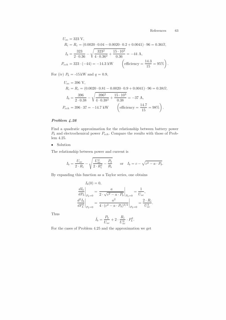
References 63
Uoc = 323 V,
Ri = Rc = (0.0020 · 0.04− 0.0020 · 0.2 + 0.0041) · 96 = 0.36Ω,
Ib =323
2 · 0.36−√
3232
4 · 0.362+
15 · 1030.36
= −44 A,
Pech = 323 · (−44) = −14.3 kW
(efficiency =
14.3
15= 95%
).
For (iv) Pb = -15kW and q = 0.9,
Uoc = 396 V,
Ri = Rc = (0.0020 · 0.81− 0.0020 · 0.9 + 0.0041) · 96 = 0.38Ω,
Ib =396
2 · 0.38−√
3962
4 · 0.382+
15 · 1030.38
= −37 A,
Pech = 396 · 37 = −14.7 kW
(efficiency =
14.7
15= 98%
).
Problem 4.26
Find a quadratic approximation for the relationship between battery powerPb and electrochemical power Pech. Compare the results with those of Prob-lem 4.25.
• Solution
The relationship between power and current is
Ib =Uoc
2 · Ri−
√U2oc
2 ·R2i
−Pb
Rior Ib = c−
√c2 − a · Pb.
By expanding this function as a Taylor series, one obtains
Ib(0) = 0,
dIbdPb
∣∣∣∣Pb=0
=a
2 ·√c2 − a · Pb
∣∣∣∣Pb=0
=1
Uoc,
d2IbdP 2
b
∣∣∣∣Pb=0
=a2
4 · (c2 − a · Pb)3/2
∣∣∣∣Pb=0
=2 · Ri
U3oc
.
Thus
Ib =Pb
Uoc+ 2 ·
Ri
U3oc
· P 2b .
For the cases of Problem 4.25 and the approximation we get
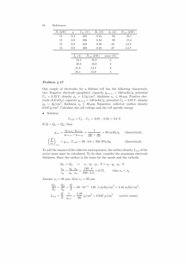
64 References
Pb (kW) q Uoc (V) Ri (Ω) Ib (A) Pech (kW)
15 0.2 323 0.45 50 16.1
15 0.9 396 0.34 39 15.4
15 0.2 323 0.36 -44 -14.3
15 0.9 369 0.38 -37 -14.7
Ib (A) Pech (kW) error (%)
52.4 16.9 5
40.3 16.0 4
-41.6 -13.4 6
-35.1 -13.9 5
Problem 4.27
One couple of electrodes for a lithium cell has the following characteris-tics: Negative electrode (graphite): capacity qrev,n = 340mAh/g, potentialUn = 0.25V, density ρn = 2.2 g/cm3, thickness sn ≤ 80µm. Positive elec-trode (LiCoO2): capacity qrev,p = 140mAh/g, potential Up = 3.85V, densityρp = 4g/cm3, thickness sp ≤ 80µm. Separator, collector: surface density0.047 g/cm2. Calculate the cell voltage and the cell specific energy.
• Solution
Ucell = Up − Un = 3.85− 0.25 = 3.6 V.
If Q = Qn = Qp, then
qrev =qrev,n · qrev,pqrev,n + qrev,p
=1
1340 + 1
140
= 99 mAh/g (theoretical),
(E
m
)
rev
= qrev · Ucell = 99 · 3.6 = 356 Wh/kg (theoretical).
To add the masses of the collector and separator, the surface density Lact of theactive mass must be calculated. To do that, consider the maximum electrodethickness. Since the surface is the same for the anode and the cathode,
Qn = Qp → sn · qn · ρn · S = sp · qp · ρp · Ssnsp
=qp · ρpqn · ρn
=140 · 4340 · 2.2
= 0.75, thus sn < sp
Assume sp = 80 µm, then sn = 60 µm.
Qn
Sn=
Qp
Sp=
Q
S= 80 · 10−4 · 140 · 4 mAh/cm2 = 4.48 mAh/cm2,
Lact =Q
S·
1
qrev=
4.48
99g/cm2 = 0.045 g/cm2 (active mass).
References 65
Add the mass of the separator to obtain
L = Lact + Lsep = 0.045 + 0.047 = 0.092 g/cm2.
The practical specific capacity qcell is thus
qcell =Q
S·1
L=
4.48
0.092= 49 mAh/g (practical),
or approximatly 50% of the theoretical capacity. The practical energy densitye is (
E
m
)
cell
= 3.6 · 49 = 176 Wh/kg (practical).
The pack specific energy will be even lower.
Problem 4.28
Develop an equation for the battery apparent capacity as a function of thecurrent for constant current discharge using the battery modeling equations ofSection 4.5.2. Then evaluate the apparent capacity of a battery with nominalcapacityQ0 = 72Ah, κ4 = −0.005, κ2 = 1.22, at C/10, C1, and C10 discharge.
• Solution
Ub = Uoc −Ri · Ib = (κ1 + κ2 · ξ)− (κ3 + κ4 · ξ) · Ib, with κ4 < 0
ξ = −IbQ∗
0
,
thus
Ub = −κ2 ·IbQ∗
0
+ κ4 ·I2bQ∗
0
= −c,
Ub(t) = Ub(0)− c · t, where Ub(0) = κ1 + κ2.
The discharge ends when Ub(tf ) = Ucut, thus for
tf =Ub(0)− Ucut
c.
The capacity or Ah rate is
Q0 = Ib · tf = Q∗0 ·
Ub(0)− Ucut
κ2 − κ4 · Ib,
which is dependent on Ib. To calculate Q0(Ib)/Q0(I∗b ), define Kc = 1−κ4/κ2 ·I∗b . One finds that
Q0
Q∗0
=Kc
1 + (Kc − 1) · IbI∗
b
,
66 References
that is (4.58) with n = 2.The nominal capacity must be retrieved for very slow currents, ideally
when I∗b = 0, as
Q∗0 = Q∗
0 ·Ub(0)− Ucut
κ2= Q∗
0 ·κ1 + κ2 − Ucut
κ2,
from whence it must be Ucut = κ1. The dependency Q0(Ib) can be rewrittenas
Q0(Ib) =Q∗
0
1 + e · Ib, where e =
|κ4|κ2
.
In the numerical case, e = 0.005/1.22 = 0.0041 The C/10 current is 72/10 =7.2 A. For this current, the capacity Q0 is
Q0 =72
1 + 0.0041 · 7.2= 70 Ah (97% of the nominal capacity)
and the discharge time tf is
tf =70
7.2= 9.7 h.
For a C1 current = 72 A,
Q0 =72
1 + 0.0041 · 72= 56 Ah (77% of the nominal capacity),
tf =56
72= 0.78 h = 46 min.
For a C10 current = 720 A,
Q0 =72
1 + 0.0041 · 720= 18 Ah (25% of the nominal capacity),
tf =18
720= 0.025 h = 1.5 min.
Problem 4.29
Verify that the round-trip efficiency of a battery under constant currentdischarge-charge and for varying parameters Uoc, Ri as described in Sec-tion 4.5.2 has the same form as (4.82) but with Uoc and Ri calculated forξ = 0.5.
• Solution
The energy discharged Ed is
Ed = Ib ·∫ tf
0Uoc(ξ)−Ri(ξ) · Ib dt =
= Ib ·∫ tf
0(κ1 + κ2 · ξ)− (κ3 + κ4 · ξ) · Ib dt.
References 67
Since ξ(t) = 1− Ib/Q0 · t under constant current discharge,
Ed = Ib·
[
κ1 · tf + κ2 ·
(
tf −Ib · t2f2 ·Q0
)
− κ3 · tf · Ib − κ4 · Ib ·
(
tf −Ib · t2f2 ·Q0
)]
.
Since tf = Q0/Ib,
Ed = Ib ·[κ1 · tf + κ2 ·
(tf −
tf2
)− κ3 · tf · Ib − κ4 · Ib ·
(tf −
tf2
)]=
= Ib · tf ·[κ1 +
κ22
− κ3 · Ib − κ4 ·Ib2
],
which is equal to
Ed = Ib · tf ·(Uoc, 12
−Ri, 12· Ib)
Similarly for Ec,
Ec = |Ib| · tf ·(Uoc, 12
+Ri, 12· |Ib|
),
and thus
ηb =Uoc, 12
−Ri 12· Ib
Uoc, 12+Ri, 12
· |Ib|.
Supercapacitors
Problem 4.31
Derive Equation (4.117).
• Solution
Psc is considered as a constant. By differentiating (4.116) one obtains
2 · Usc ·d
dtUsc +
IscCsc
· Usc −Qsc
Csc·d
dtUsc = 0,
where the second of (4.115) has been used. By solving (4.116) for Qsc, oneobtains
Qsc =Csc
Usc· (Psc · Rsc + U2
sc),
thus
2 · Usc ·d
dtUsc +
Psc
Csc−
d
dtUsc ·
(Psc ·
Rsc
Usc+ Usc
).
Since 2 · Usc · dUsc/dt = d/dt(U2sc), one obtains
d
dtU2sc+
Psc
Csc−Psc · Rsc · d
dtU2sc
2 · U2sc
−ddtU
2sc
2= 0 ⇒
d
dt
U2sc
2+Psc
Csc−Psc · Rsc · d
dtU2
2 · U2sc
= 0,
from whence (4.117) follows. For Rsc = 0 it is found that dEsc/dt = d/dt(Csc ·U2sc/2) = −Psc (Psc positive during discharge).
68 References
Problem 4.32
Derive an analytical solution for the discharge of a supercapacitor with max-imum power. Then verify the solution with the data of Figure 4.42.
• Solution
At max power
Psc =Q2
sc
4 ·Rsc · C2sc,
then from (4.118)
Usc =Qsc
2 · Csc,
from (4.115)
Rsc · Isc =Qsc
Csc−
Qsc
2 · Csc=
Qsc
2 · Csc
anddQsc
dt= −
Qsc
2 ·Rsc · Csc.
Thus
Qsc(t) = Q0 · e−t
2·Csc·Rsc ,
Isc(t) =Q0
2 · Csc · Rsc· e−
t2·Csc·Rsc ,
Usc(t) =Q0
2 · Csc· e−
t2·Csc·Rsc ,
Psc(t) =Q2
0
4 ·Rsc · C2sc
· e−t
Csc·Rsc .
For t = 2 s, Csc = 12.5 F, Rsc = 0.08Ω, and Q0 = 800 C, find
Qsc(t) = 800 · e−2
2·12.5·0.08 = 294 C,
Isc(t) =800
2 · 12.5 · 0.08· e−
22·12.5·0.08 = 147 A,
Usc(t) =800
2 · 12.5· e−
22·12.5·0.08 = 12 V,
Psc(t) =8002
4 · 0.08 · 12.52· e−
212.5·0.08 = 1.7 kW.
Problem 4.33
Yet another definition of supercapacitor efficiency that is sometimes found(e.g., in [222]) is
ηsc,d = 1− 2τ
tf,
References 69
during discharge at constant current, and
ηsc,c =1
1 + 2 τtf
,
during charge at constant current, where τ = Csc · Rsc and tf has the samemeaning as in the text. Explain this definition.
• Solution
The energy amount that can be obtained from a fully-charged supercapacitorwith constant-current discharge in the ideal case of negligible resistance isobtained from (4.119) as
Ed,id =Q2
0
2 · Csc,
which coincides with the maximum stored energy defined in (4.129). By defin-ing the efficiency as
ηsc,d =Ed
Ed,id,
find the value in the problem statement.For charge, define the efficiency as
ηsc,c =|Ec,id||Ec|
,
and find the value in the problem statement with |Ec,id| = Ed,id.
Electric Power Links
Problem 4.34
Consider again Problem 4.9 and account for a battery internal resistance of0.025Ω.
• Solution
Combine DC motor equations and battery equations with Ub = Um andIb = Im. The relationship linking the motor torque, speed, and the DC–DCconverter duty cycle is
α · Uoc −(Ra + α2 ·Rb) · Tm
κa− κi · ωm = 0.
The flux weakening region limit is obtained for α = 1 as 0.3 · Tm + 0.25 ·ωm = 50V (axis intercepts at 200 rad/s and 167Nm). The current limit isobtained by setting α = 1 and ωm · Tm = Pm,max. The result is the same asin Problem 4.9 but now Ra should be replaced by Ra + Rb = 0.075Ω. Thenew solution is Im,max = 93A (increase).
70 References
In the case (i) only the calculation of α changes, since Ua = 28V andIa = 60A are still admissible values. Knowing that
Ub = Uoc −Rb · Ib,
α =Ua
Ub=
IbIa
,
one obtainsUa = Uoc · α−Rb · Ia · α2,
from whence α = 57% (increase) and correspondingly Ub = 49V, Ib = 34A(increase). Alternatively, α can be directly calculated from the general equa-tion above.
For the case (ii) again Ra is replaced by the sum of the two resistances. Theduty cycle is still fixed at α = 100% and the flux is now κi = κa = 0.14Wb.Thus the flux weakening increases.
Problem 4.35
For an electric drive including a battery, a step-down DC–DC converter (chop-per), and a DC motor, calculate the duty cycle that maximizes the regeneratedpower during braking. Calculate the corresponding motor current, using thedata presented in Problem 4.9.
• Solution
The limitation is imposed by the step-down converter for which R = Ua/Ub =1− α. Evaluate R as a function of ωm and Ia:
R · Uoc −Rb ·R2 · Ia −Ra · Ia − κi · ω = 0.
For R = 0,
Ia = −κi ·ω
Ra,
but Ib = R · Ia = 0 (no recuperation). For R = κi ·ωm/Uoc, Ia = 0 and Ib = 0(again no recuperation). Thus there must be a value R > 0 that maximizesthe recuperated power. The power is
Pa = Pb = Ia · (Ra · Ia + κi · ωm) = Ra · I2a + κi · ωm · Ia,dPa
dIa= 2 · Ra · Ia + κi · ωm = 0 ⇒ Ia = −κi ·
ωm
2 · Ra= Ia,min.
For this value of current
R · Uoc +Rb
2 ·Ra· κi · ωm · R2 −
κi · ω2
= 0 ⇒ Rmin.
And inserting the data of Problem 4.9,
References 71
Ia,min = −κi · ωm
2 · Ra= −
0.25 · 1002 · 0.05
= −250 A,
R2 · (Rb · Ia,min)− u · Uoc +Ra · Ia,min + κi · ω = 0 ⇒ Rmin = 24%.
Problem 4.36
Consider an electric drive including a battery, a boost DC–DC converter and amotor. Derive a relationship between the maximum torque curve of the motorand the converter ratio, assuming that for ωm > ωb, Pmax ≈ Umax · Imax.Conceive a strategy to perform quasistatic simulations in this case.
• Solution
A simplified expression for the motor maximum torque is
Tmax = mink · Imax, Pmax/ωm
where the constant k is given by κa in DC motors and by 3/2·p·ϕm in PMSMs.The maximum power is Pmax = Imax ·Umax where Umax is the voltage at theDC side of the motor. One obtains
Pmax = Umax · Imax = Imax ·R · (Uoc −Rb ·R · Imax) = f(R)
In backward modeling, the required torque Tm has to be saturated by themaximum value Tmax. However, this value depends on R. Physically, there isone value of R that realizes the desired speed and torque (see a similar situa-tion in Problem 4.34). For simulation purposes, one could map the conversionratio as a function of motor speed and torque and then feed the maximumtorque map. Alternatively, Tmax could be mapped as a function of speed andvoltage Umax and the latter calculated as Ub · Ib/Imax.
Problem 4.37
Consider a semi-active power link with a battery, a supercapacitor, an elec-tric motor, and a DC–DC converter on the supercapacitor branch. Derive ananalytical relationship between the control factor u (4.132) and the DC–DCconverter voltage ratio R. Calculate the values of R to obtain a pure bat-tery supply (u = 0) or a pure supercapacitor supply (u = 1). Describe thesupercapacitor on a quasistatic basis, i.e.,
Csc ·Us0 − Usc
τ= −Isc,
where τ is the time step.
• Solution
72 References
The battery equation is Ub = Uoc −Rb · Ib. The DC link equations are Um =R · Usc = Ub. Additionally, Ib + Isc/R = Im. The supercapacitor equation isgiven in the problem formulation. There are five equations in the six variablesUb, Ib, Usc, Isc, Um, Im. However, in dynamic modeling Im is given from thedownstream powertrain. Thus all the other quantities can be calculated as afunction of R. The result is
Um = Ub =Uoc
Rb+ C
τUs0R − Im
1Rb
+ CτR2
,
from whence Usc, Isc, and Ib are calculated as well. The supercapacitor powerPsc is
Psc = UscIsc =Um
R
C
τ(Us0 − Usc)
and the control ratio u is
u =Psc
Pm=
1
Im
(CUs0
τR−
C
τR2
Uoc
Rb+ C
τUs0R − Im
1Rb
+ CτR2
)
= u(R, Im).
To find u = 0, the DC–DC converter must be regulated such as
R =Uoc −RbIm
Us0.
To obtain u = 1, the DC–DC converter must be regulated such as R is thesolution of the quadratic equation
τImR2 − CUs0R + CUoc = 0.
The condition to have a solution is
(CUs0)2 − 4τImCUoc > 0.
Therefore, pure supercapacitor operation is allowed for
Im <CU2
s0
4τUoc.
Torque Couplers
Problem 4.38
Consider a through-the-road parallel hybrid. The torque coupling has the fol-lowing characteristics: transmission ratio between the rear-axle motor and thewheels γm = 11, transmission ratios between the front-axle engine and thewheels γe = 15.02, 8.09, 5.33, 3.93, 3.13, 2.59, wheel radius rwh = 31.7 cm.Moreover, Tm,max = −Tm,min = 140Nm, Pm,max = −Pm,min = 42kW, en-gine speed limited to ωe,max = 4500 rpm, engine maximum torque Te,max =
References 73
1.34 · 10−5 · ω3e − 0.0149 · ω2
e + 4.945 · ωe − 243 (Nm), engine minimumtorque Te,min = −20Nm. For a driving situation with V = 30m/s andTwh = 675Nm, determine the limits imposed by the motor operation on theengine operation.
• Solution
The engine speed for various gears is
ωe = γe ·V
rwh= 947, 510, 336, 248, 197, 163 rad/s.
Since ωe,max = 471 rad/s only the third to sixth gears are admissible. Theengine maximum torque Te,max for the four admissible speeds is
Te,max = 242, 270, 255, 225 Nm.
However, the torque coupling equation reads
Te · γe + Tm · γm = Twh.
Since Tm ≥ Tm,min, consequently,
Te ≤Twh − γm · Tm,min
γe= 259, 351, 441, 533.
In all cases, the motor imposed limits overshadow the engine physical limitsduring generating operation. For motoring operation,
Te ≥Twh − γm · Tm,max
γe= 1.6, 2.1, 2.7, 3.2.
that prevents, e.g., purely electric operation (Te = 0).
Power Split Devices
Problem 4.39
Consider a power-split combined hybrid powertrain with a planetary gear setlinking the engine, the generator, and the output shafts with the followingWillis relation
ωg = 3.6 · ωe − 2.6 · ωf .
The second electric machine is mounted directly on the output shaft with-out any reduction gear. The generator has the following characteristics (bothin motor and in generator modes): maximum torque = 160 Nm, maximumpower = 25 kW, maximum speed = 1200 rad/s. The motor has the followingcharacteristics (both in motoring and in generating mode): maximum torque= 400Nm, maximum power = 25kW, and maximum speed = 700 rad/s. The
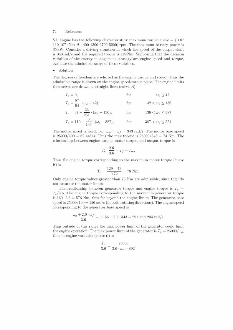
74 References
S.I. engine has the following characteristics: maximum torque curve = 0 87110 107Nm @ 400 1300 3700 5000 rpm. The maximum battery power is35 kW. Consider a driving situation in which the speed of the output shaftis 343 rad/s and the required torque is 129Nm. Supposing that the decisionvariables of the energy management strategy are engine speed and torque,evaluate the admissible range of these variables.
• Solution
The degrees of freedom are selected as the engine torque and speed. Thus theadmissible range is drawn on the engine speed-torque plane. The engine limitsthemselves are drawn as straight lines (curve A)
Te = 0, for ωe ≤ 42
Te =87
94· (ωe − 42), for 42 < ωe ≤ 136
Te = 87 +23
251· (ωe − 136), for 136 < ωe ≤ 387
Te = 110−3
136· (ωe − 387), for 387 < ωe ≤ 524
The motor speed is fixed, i.e., ωm = ωf = 343 rad/s. The motor base speedis 25000/400 = 62 rad/s. Thus the max torque is 25000/343 = 73 Nm. Therelationship between engine torque, motor torque, and output torque is
Te ·2.6
3.6= Tf − Tm.
Thus the engine torque corresponding to the maximum motor torque (curveB) is
Te =129− 73
0.72= 78 Nm.
Only engine torque values greater than 78 Nm are admissible, since they donot saturate the motor limits.
The relationship between generator torque and engine torque is Tg =Te/3.6. The engine torque corresponding to the maximum generator torqueis 160 · 3.6 = 576 Nm, thus far beyond the engine limits. The generator basespeed is 25000/160= 156 rad/s (in both rotating directions). The engine speedcorresponding to the generator base speed is
ωg + 2.6 · ωf
3.6= ±156 + 2.6 · 343 = 291 and 204 rad/s.
Thus outside of this range the max power limit of the generator could limitthe engine operation. The max power limit of the generator is Tg = 25000/ωg,thus in engine variables (curve C) is
Te
3.6=
25000
3.6 · ωe − 892.
References 75
The intersection of curve C with the curve Te = 110 Nm is at 475 rad/s.To be more precise, the intersection should be made with the fourth branchof the curve A, leading to a quadratic equation.
Neglecting in a first approximation the motor and generator losses, thebattery power is Pb = Pm − Pg = Pf − Pe. The output power is Pf =129 · 343 = 44247 W. Thus the limit Pb = 35 kW in engine variables becomesωe · Te = 44247 W − 35000 W = 9247 W (curve D). The intersection withcurve B is at 118 rad/s. The curve A at this engine speed gives 70Nm, whichis below curve B. Thus the battery constraint is not active at these drivingconditions. All the other limits (generator minimum torque, motor minimumtorque) are not active as well.
The engine admissible range is thus between curve B (Te = 78 Nm), curveA (between ωe = 126 rad/s and 475 rad/s), and curve C (between ωe =475 rad/s and 524 rad/s).
million cars
all countries
USA
800
400
1980 2000 year
Fig. 10.11. Schematic representation of the development of the number of passen-ger cars operated worldwide.
Problem 4.40
Derive the coupling matrix for the four torque levels of a PSD from the el-ements of the kinematic matrix in the case of quasistatic modeling. Do thesame in the case of forward modeling, i.e., derive (4.166).
• Solution
In backward modeling the kinematic matrix generally reads
ωe = A · ωf +B · ωg,
ωm = C · ωf +D · ωg.
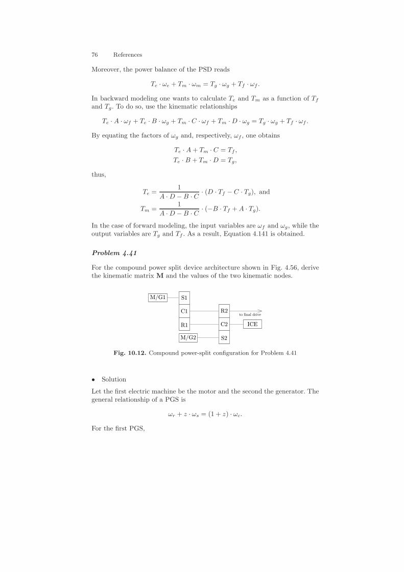
76 References
Moreover, the power balance of the PSD reads
Te · ωe + Tm · ωm = Tg · ωg + Tf · ωf .
In backward modeling one wants to calculate Te and Tm as a function of Tf
and Tg. To do so, use the kinematic relationships
Te · A · ωf + Te ·B · ωg + Tm · C · ωf + Tm ·D · ωg = Tg · ωg + Tf · ωf .
By equating the factors of ωg and, respectively, ωf , one obtains
Te ·A+ Tm · C = Tf ,
Te · B + Tm ·D = Tg,
thus,
Te =1
A ·D −B · C· (D · Tf − C · Tg), and
Tm =1
A ·D −B · C· (−B · Tf +A · Tg).
In the case of forward modeling, the input variables are ωf and ωg, while theoutput variables are Tg and Tf . As a result, Equation 4.141 is obtained.
Problem 4.41
For the compound power split device architecture shown in Fig. 4.56, derivethe kinematic matrix M and the values of the two kinematic nodes.
S1
C1
R1
M/G2
M/G1
ICE
R2
C2
S2
to final drive
Fig. 10.12. Compound power-split configuration for Problem 4.41
• Solution
Let the first electric machine be the motor and the second the generator. Thegeneral relationship of a PGS is
ωr + z · ωs = (1 + z) · ωc.
For the first PGS,
References 77
ωe + z1 · ωm = (1 + z1) · ωf .
For the second PGS,
ωf + z2 · ωg = (1 + z2) · ωe.
Thus the kinematic matrix is A = 1/(1 + z2), B = z2/(1 + z2), C = (z1 +z2 + z1z2)/z1(1 + z2), D = −1/z1(1 + z2). The two nodes are calculated (seeProblem 4.42) as K1 = 1/(1 + z1) and K2 = 1 + z2).
Problem 4.42
Derive equation (4.167) for Kv as a function of K and equation (4.168) for ras a function of K, including the definitions of K1 and K2.
• Solution
We use the definition of M as in Problem 4.40. By defining K = ωf/ωe, wehave
ωg/ωe = A ·K +B and ωm/ωe = C ·K +D.
Thus,
Kv =ωm
ωg=
C ·K +D
A ·K +B=
D
B·(
1− KK1
)
1− KK2
from whence the definition of K1 = −D/C and K2 = −B/A. The power splitratio is
r =ωg
ωe·Tg
Te=ωm
ωe·Tm
Te.
By using the torque matrix calculated in Problem 10,
r = (A ·K +B) ·D · Tf
Te+ C
B · C −A ·D= (C ·K +D) ·
B · Tf
Te+A
B · C −A ·D.
Equating the last two equations and defining Tf/Te = X , derive that
(D ·X + C) · (A ·K +B) = (C ·K +D) · (B ·X +A)
from whence
X · (D · (A ·K +B)−B · (C ·K +D)) = A · (C ·K +D)− C · (A ·K +B)
⇒ X · (A ·D ·K −B · C ·K) = A ·D −B · C,
thus X = 1/K. Hence,
r =1
K·(C ·K +D) · (B +A ·K)
B · C −A ·D=
1
K·D · B ·
(1 + KK1
) · (1 + KK2
)
B · C −A ·D.
As B · C −A ·D can be written as
D · B ·(C
D−
A
B
)= D ·B ·
(1
K2−
1
K1
),
equation (4.143) is obtained.
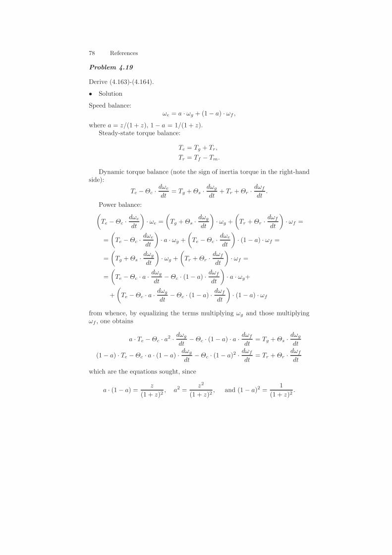
78 References
Problem 4.19
Derive (4.163)-(4.164).
• Solution
Speed balance:ωe = a · ωg + (1− a) · ωf ,
where a = z/(1 + z), 1− a = 1/(1 + z).Steady-state torque balance:
Te = Tg + Tr,
Tr = Tf − Tm.
Dynamic torque balance (note the sign of inertia torque in the right-handside):
Te −Θc ·dωe
dt= Tg +Θs ·
dωg
dt+ Tr +Θr ·
dωf
dt.
Power balance:(Te −Θc ·
dωe
dt
)· ωe =
(Tg +Θs ·
dωg
dt
)· ωg +
(Tr +Θr ·
dωf
dt
)· ωf =
=
(Te −Θc ·
dωe
dt
)· a · ωg +
(Te −Θc ·
dωe
dt
)· (1 − a) · ωf =
=
(Tg +Θs ·
dωg
dt
)· ωg +
(Tr +Θr ·
dωf
dt
)· ωf =
=
(Te −Θc · a ·
dωg
dt− Θc · (1− a) ·
dωf
dt
)· a · ωg+
+
(Te −Θc · a ·
dωg
dt−Θc · (1 − a) ·
dωf
dt
)· (1− a) · ωf
from whence, by equalizing the terms multiplying ωg and those multiplyingωf , one obtains
a · Te −Θc · a2 ·dωg
dt−Θc · (1− a) · a ·
dωf
dt= Tg +Θs ·
dωg
dt
(1− a) · Te −Θc · a · (1− a) ·dωg
dt−Θc · (1− a)2 ·
dωf
dt= Tr +Θr ·
dωf
dt
which are the equations sought, since
a · (1− a) =z
(1 + z)2, a2 =
z2
(1 + z)2, and (1 − a)2 =
1
(1 + z)2.
References 79
Problem ??
Extend equations (4.149)-(4.150) to the case where there are losses in theplanetary gearset.
• Solution
Assume that es and er are the efficiencies of the contacts carrier-sun andcarrier-ring, respectively, the power balance neglecting the inertia terms issimply written as
Pe =1
es· Pg +
1
er· Pr,
Te · ωe =Tg
es· ωg +
Tr
er· ωf , from whence
Tg = es · a · Te, and
Tr = er · (1− a) · Te, where a =z
1 + z.
The lost power Plost is
Plost = Te · ωe − Tg · ωg − Tr · ωf =
= a · Te · ωg · (1− es) + (1− a) · Te · ωf · (1− er).
Non-electric Hybrid Propulsion Systems
Hybrid-inertial Powertrains
Problem 5.1
Derive a Ragone curve similar to (5.1) and (5.2) for a flywheel battery. Thenevaluate the maximum energy and power. Use a simplified expression for theloss power of the type Pl = R · ω2
f .
• Solution
Assume constant power output of the flywheel and assume the flywheelstarts at speed ω0.newline
a) Dynamics of the flywheelFor constant power Pf , the dynamic equation:
Θf · ωf · ωf = −Pf −R · ω2f ,
which can be rewritten as the following integral:
80 References
Θf · dωf
Pf +R · ω2f
= −dt
Θf
2R · d(Rω2f + Pf )
(Rω2f + Pf )
= −dt
Θf
2Rln[Pf +Rω2
f(∞)] ∣∣t∞
t0= −t
∣∣∞0
Θf
2Rln
[Pf +Rω2
f (∞)
Pf +Rω2f(0)
]
= −(t∞ − t0)
By setting integral limits from t = 0,ωf = ω0 to t = t∞,ωf = 0 yields
Θf
2Rln
[Pf +Rω2
f(∞)
Pf
]
= −(t∞)
t∞ = τ · ln(1 +R · ω20/Pf ).
where τ # Θf/(2R).b) Energy delivery
Ef = Pf · t∞
= Pf ·
⎧⎨
⎩−Θf
2R· ln
⎡
⎣ 1
1 +Rω20
Pf
⎤
⎦
⎫⎬
⎭
=Θf
2R· Pf ln
[1 +R
ω20
Pf
].
c) Initial energy availableThe initial energy stored in the flywheel is
E0 = 1/2 · Θf · ω20 .
Thus the efficiency can be calculated as
ηf =Ef
E0=
Pf
R · ω20
· ln[1 +
R · ω20
Pf
].
DiscussionIf we plot out the Ragone curve Ef = Ef (Pf ), it appears to be amonotonously increasing curve, contrarily to battery and supercapaci-tors. That is, the larger is the power, the larger is the energy that canbe extracted from the flywheel and thus its efficiency.
References 81
Problem 5.2
Dimension a flywheel for the following application (F1 KERS): Pmax = 60kW,Emax = 500kJ, ωmax = 60000 rpm. Assume β = 0.5, ρ = 1658kg/m3 (carbonfiber), ρ0.8a η0.2a = 0.48 (sealed flywheel).
• Solution
Assume β denotes the the geometric ratio of the wheel width over thewheel diameter; d = 0.2 [m], and q denotes the ratio between inner andouter diameters of the flywheel rings.
a) Calculate the moment of inertiaThe maximum speed is ωmax = 60000 rpm = 60000 · 2π/60 = 6283 rad/s.From the maximum energy, the moment of inertia can be calculated with
Θf =2 · Emax
ωmax= 2 · 500 · 103/(6283)2 = 0.0233 kg · m2.
b) Find the flywheel diameterBy setting Pl,a = Pmax and neglecting bearing losses, the diameter isfound from (5.5) by setting Pl,a = Pmax, i.e.,
0.04 · ρ0a.8 · η0a.2 · u2.8(t) · (β + 0.33) = Pl,a(t) = Pmeax
0.04 · 0.48 · d4.6 · (6283/2)2.8 · 0.83 = 60 · 103,
from whence d ≈ 0.2m. Thus b = β · d = 0.5 · 0.2 = 0.1m.c) Dimension the flywheel mass with material property
Using (5.7), find the geometric ratio q from the equation:
Θf =π
2· ρ · b
d4
16(1 − q4)
0.026 = 3.14 · 1658/32 · (1− q4) · 0.1 · 0.24,
from whence q = 0.4069.The mass is obtained from (5.8) as
mf = ρ ·∫ rout
rin
1 · (2πr)dr
mf = πρbd2
4· (1 − q2)
mf = 0.1 · 0.22 · 3.14 · 1658 · (1− 0.40692)/4 = 4.346 kg.
Problem 5.3
Evaluate the charging efficiency of the flywheel of Problem 5.2 for a brakingat maximum power for 2 s. Evaluate the round-trip efficiency.
82 References
• Solution
a) Charging efficiency
(i) estimate the coefficient of loss power using maximum achievable powerDuring charging, the flywheel dynamics reads Θf ·ωf ·ωf = Pf−R·ω2
f .Using the data of Problem 5.2, an approximation for R could be
R = Pmax/ω2max = 60 · 103/(60000 · 2π/60)2 = 0.0015.
Thus, the charging speed trajectory ωf satisfies:
θf cdotωf · ωf = Pf −R · ω2f
which gives, τ ln
[Pf −R · ω2
f (∞)
Pf −R · ω2f (0)
]
= −(t∞ − t0)
By definition, τ # Θf/(2R) = 8.332 s. Therefore, beginning at rest,the speed profile is as follows, with the maximum braking power charg-ing the flywheel for 2 s:
ωf =Pf
R
[1− e−
tτ
],
ωf |t=2 s =
√60× 103
1.52× 10⁻³
[1− e−
28.332
]= 2902 rad/s.
(ii) Charging efficiencyCharging efficiency is the ratio of available energy storage to availableenergy input from regenerative braking:
Ein =Pf · t
Eout =1
2Θf ω
2f =
1
2Θf
Pf
R
[1− e−
tτ
]
ηc =Eout
Ein=
Θf
2Rt
[1− e−
tT
].
=8.332 s
2 s
[1− e−
2 s8.332 s
]= 88.90%.
b) Calculate discharge and thus roundtrip efficiencyThe initial speed for discharging equals the final speed of charging:
ω0,disch = ωf,ch = 2902 rad/s.
Thus, the total discharging energy equals:
Ef,disch =Θ
2RPf ln
[
1 +R · ω2
0,disch
Pf
]
.
References 83
With the energy storage in the flywheel, the discharging efficiency can becalculated:
ηdisch =Ef,disch
Eout=
⎧⎪⎨
⎪⎩
ln[1 +
R·ω20,disch
Pf
]
1− e−tchτ
⎫⎪⎬
⎪⎭= 90.64%
Finally, the round-trip efficiency is therefore η = ηch · ηdisch = 80.58%.DiscussionGenerally, the maximum energy of flywheel is used to estimate the momentof inertia and mass, while the maximum power is used to estimate thecoefficient of loss power.
Problem 5.4
Evaluate the CVT ratio ν(t) during a deceleration of a vehicle equipped witha flywheel-based KERS and the opening time of the clutch. Use the flywheeldata of Problem 5.3. The flywheel is connected to the input stage of theCVT through a fixed-reduction gear with ratio 8.33. Final drive and wheel
ratio(
γfd
rw
)= 13. Initial conditions: v(0) = 80km/h, ωf (0) = 10000 rpm,
mv = 600kg, braking time 2 s (assume a constant braking power), CVT rangeνmax/νmin = 6.
• Solution
a) Calculate the range of CVT ratioAs for the initial speed,
ν(0) =ωf (0)
γf · ν(0) · γfd
rw
=10000× 2 π/60
8.33 · 80/3.6 · 13= 0.4352.
Therefore, given the CVT range, the maximum CVT ratio is as follows:
ν(t) = ν(0)×νmax
νmin= 6× 0.4352 = 2.611.
b) List equations from the vehicle sideGiven that the vehicle speed trajectory during decceleration is
v2(t) = v2(0)− 2Pb · tb/mv
, where Pb is the constant braking power which brings the vehicle approx-imately towards standstill. Thus, the average braking power is
Pb =mv · ω2
tb= 1/2 · 600 · (80/3.6)2/2 = 74.07 kW.
The corresponding final speed at the clutch opening time equals:
v2(tc) =
(80
3.6
)2
−2× 74.07× 103 · tc
600.
84 References
c) List equations from the flywheel sideAccording to the result of Problem 5.3:
Pf
R− ω2
f (t) =
[Pf
R− ω2
f (0)
]· e−
tτ .
Using intemediate results from Problem 5.3, the following values areknown:
Pf = 60 kW, R = 0.01520 kg · · ·m2, τ = 8.332 s.
Equations from the flywheel side can be established by substituting valuesin.
d) Solve equations with the CVT ratio constraint
⎧⎪⎪⎨
⎪⎪⎩
ν(tc) = 2.611 = ωf (tc)
ν(tc)·γf ·γfdrw
ω2f(tc) = −
[Pf/r − ω2
f (0)]· e− t
τ +Pf/R
v2(tc) = v2(0)− 2Pb · tc/mv
Substituting one speed with the other, we get:
(2.611×
80
3.6× 8.33× 13
)2
=ω2f (tc)
v2(tc). (*)
Eliminate the second unknown variable and make equations of tc only:
1
3.948× 10⁷
Pf/R−
[Pf/R− ω2
f(0)]· e−
tcτ
= v2(0)− 2× Pb × tc/mv.
(10.26)The solution is therefore:
⎧⎪⎨
⎪⎩
tc = 1.9999 s ≈ 2 s
ωf (tc) = 1431 rad/s = 13660 rpm
v(tc) = 0.1648m/s.
DiscussionAfter the clutch opening time t > tc, the clutch is open and the vehiclecan further decelerate util rest, with the help of tyre friction power.
Hybrid-hydraulic Powertrains
Problem 5.5
Derive a Ragone curve similar to (5.1) and (5.2) for a hydraulic accumulator.Show that for high power this definition is equivalent to that adopted in thetext.
• Solution

References 85
a) Energy balanceEstablish the accumulator’s energy balance for Ragone Curve:
⎧⎪⎨
⎪⎩
E = mg · cv · ddt θg(t) = −pg(t) · d
dt Vg(t)− hAw(θg(t)− θw)ddt Vg(t) = Qh(t)
Pg(t) =mg Rg θg(t)
Vg(t).
b) Power outputAs from the textbook, the power of a hydraulic accumulator is outputthrough the change of pressurized flow:
Ph = pg(t) ·Qh(t).
Therefore, given that E = mg cv θg(t), rewrite the energy balance as fol-lows:
E = −Ph −hAw
mg cv· E + hAw θw.
Let τ = mg cvhAw
, and E∗ = E + τ (Ph − hAw θw), then we have:
dE∗
E∗= −
dt
t.
c) Solve ODE with initial and final conditions.
Assume constant power output.
Assume starting of the cycle is defined as point “B”, while the end ofpower output is reached when gas temperature equals liquid temperature.
E|t=0 = mgcv,gθBE|t=∞ = mgcv,gθw = Eh
Solving the ODE subject to these conditions, we get:
t∞ = τ · ln[Ph + (E0 − Ew)
Ph
]
So the total energy transmitted is:
Eha = Ph · t∞ = Ph · τ · ln[1 +
E0 − Ew
Ph · τ
]
d) Prove the equivalence of validityAccording to the reference cycle used for power output:
WAB = mg · cv,g (θB − θA) = E0 − Ew
. When Ph → ∞, using L’Hospital rule in limit calculation, we get:
86 References
Eha = k · (E0 − Ew) = k ·WAB,
which proves the validity of definition (5.36), as an equivalence of theRagone Curve functionDiscussion
• the energy balance ODE assuming the mode of constant power outputis a source of Ragone Curve Function;
• the Ragone Curve shows the energy is positively correlated with thepower, so the energy output is hight if the constant power level ishigher.
Problem 5.6
Derive (5.48) and (5.50).
• Solution
Fuel-Cell Propulsion Systems
Fuel Cells
Problem 6.1
For high pressures, the thermodynamic properties of gas have to be calculatedusing the Redlich–Kwong equation of state instead of the ideal gas law. TheRedlich–Kwong equation reads
p =R · ϑV − b
−a√
ϑ · V · (V + b), (10.27)
where p is pressure, R is the universal gas constant, ϑ is temperature, V isthe molar volume. The constants a and b are defined as
a =0.4275 · R2 · ϑ2/5c
pc, b =
0.08664 · R · ϑcpc
, (10.28)
where ϑc is the temperature at the critical point, and pc is the pressure atthe critical point. Using this equation of state, evaluate the gaseous densityof hydrogen at 350bar, 700 bar, when the gas temperature is 300K.
• Solution
Assume the temperature of H2 is 300K.
References 87
a) Gas states and constantsFrom thermodynamic tables, R = 8.314J/mol · K, θc = 32.97K, pc =1.293 MPa. Then, we find the constants:
a =0.4275× R2 × θ0c .4
pc
=0.4275× 8.3142 × 32.970.4
1.293× 106
= 9.251× 10⁻⁵;
b =0.08664× R× θc
pc
=0.08664× 8.314× 32.97
1.293× 106
= 1.837× 10⁻⁵.
b) when p1 = 350× 105 Pa, θ1 = 300 K.
P1 =R θ1
V1 − b−
a√θ1 · V1 · (V1 + b)
350× 105 =8.314× 300
V1 − 1.837× 10⁻⁵−
9.251× 10⁻⁵
sqrt300× V1(V1 + 1.837× 10⁻⁵)
Solve the 3rd order algebraic equation, we get:
V1 = 8.963× 10⁻⁵m3/mol;
ρ1,H2 = Mh
V1= 22.31kg/m2.
c) when p2 = 700× 105 Pa, θ2 = 300 K.
P2 =R θ2
V2 − b−
a√θ2 · V2 · (V2 + b)
700× 105 =8.314× 300
V2 − 1.837× 10⁻⁵−
9.251× 10⁻⁵
sqrt300× V2(V2 + 1.837× 10⁻⁵)
Solve the 3rd order algebraic equation, we get:V2 = 5.400× 10⁻⁵m3/mol;
ρ2,H2 = Mh
V2= 37.04kg/m3.
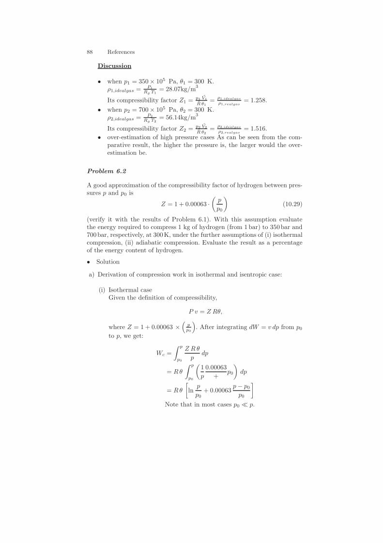
88 References
Discussion
• when p1 = 350× 105 Pa, θ1 = 300 K.ρ1,idealgas =
P1Rg T1
= 28.07kg/m3
Its compressibility factor Z1 = p1 V1
R θ1= ρ1,idealgas
ρ1,realgas= 1.258.
• when p2 = 700× 105 Pa, θ2 = 300 K.ρ2,idealgas =
P2Rg T2
= 56.14kg/m3
Its compressibility factor Z2 = p2 V2
R θ2= ρ2,idealgas
ρ2,realgas= 1.516.
• over-estimation of high pressure cases As can be seen from the com-parative result, the higher the pressure is, the larger would the over-estimation be.
Problem 6.2
A good approximation of the compressibility factor of hydrogen between pres-sures p and p0 is
Z = 1 + 0.00063 ·(
p
p0
)(10.29)
(verify it with the results of Problem 6.1). With this assumption evaluatethe energy required to compress 1 kg of hydrogen (from 1 bar) to 350bar and700bar, respectively, at 300K, under the further assumptions of (i) isothermalcompression, (ii) adiabatic compression. Evaluate the result as a percentageof the energy content of hydrogen.
• Solution
a) Derivation of compression work in isothermal and isentropic case:
(i) Isothermal caseGiven the definition of compressibility,
P v = Z Rθ,
where Z = 1+ 0.00063 ×(
pp0
). After integrating dW = v dp from p0
to p, we get:
Wc =
∫ p
p0
Z R θ
pdp
= R θ
∫ p
p0
(1
p
0.00063
+p0
)dp
= R θ
[ln
p
p0+ 0.00063
p− p0p0
]
Note that in most cases p0 ≪ p.
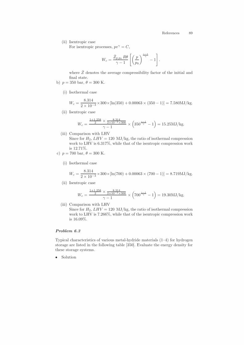
References 89
(ii) Isentropic caseFor isentropic processes, pvγ = C,
Wc =Zp,p0 Rθ
γ − 1
[(p
p0
) γ−1γ
− 1
]
.
where Z denotes the average compressibility factor of the initial andfinal state.
b) p = 350 bar, θ = 300 K.
(i) Isothermal case
Wc =8.314
2× 10−3×300×[ln(350) + 0.00063× (350− 1)] = 7.580MJ/kg.
(ii) Isentropic case
Wc =1+1.258
2 × 8.3142×10−3×300
γ − 1×(350
γ−1γ − 1
)= 15.25MJ/kg.
(iii) Comparison with LHVSince for H2, LHV = 120 MJ/kg, the ratio of isothermal compressionwork to LHV is 6.317%, while that of the isentropic compression workis 12.71%.
c) p = 700 bar, θ = 300 K.
(i) Isothermal case
Wc =8.314
2× 10−3×300×[ln(700) + 0.00063× (700− 1)] = 8.719MJ/kg.
(ii) Isentropic case
Wc =1+1.258
2 × 8.3142×10−3×300
γ − 1×(700
γ−1γ − 1
)= 19.30MJ/kg.
(iii) Comparison with LHVSince for H2, LHV = 120 MJ/kg, the ratio of isothermal compressionwork to LHV is 7.266%, while that of the isentropic compression workis 16.09%.
Problem 6.3
Typical characteristics of various metal-hydride materials (1–4) for hydrogenstorage are listed in the following table [350]. Evaluate the energy density forthese storage systems.
• Solution
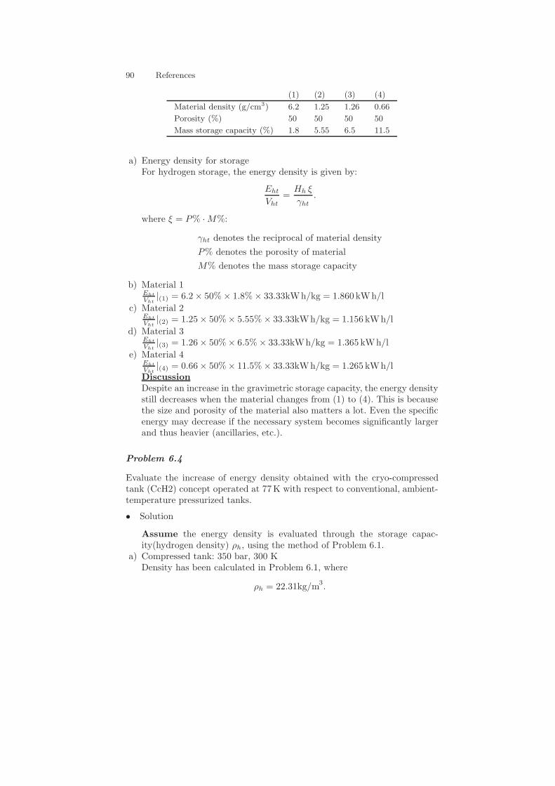
90 References
(1) (2) (3) (4)
Material density (g/cm3) 6.2 1.25 1.26 0.66
Porosity (%) 50 50 50 50
Mass storage capacity (%) 1.8 5.55 6.5 11.5
a) Energy density for storageFor hydrogen storage, the energy density is given by:
Eht
Vht=
Hh ξ
γht.
where ξ = P% ·M%:
γht denotes the reciprocal of material density
P% denotes the porosity of material
M% denotes the mass storage capacity
b) Material 1Eht
Vht|(1) = 6.2× 50%× 1.8%× 33.33kWh/kg = 1.860 kWh/l
c) Material 2Eht
Vht|(2) = 1.25× 50%× 5.55%× 33.33kWh/kg = 1.156 kWh/l
d) Material 3Eht
Vht|(3) = 1.26× 50%× 6.5%× 33.33kWh/kg = 1.365 kWh/l
e) Material 4Eht
Vht|(4) = 0.66× 50%× 11.5%× 33.33kWh/kg = 1.265 kWh/l
DiscussionDespite an increase in the gravimetric storage capacity, the energy densitystill decreases when the material changes from (1) to (4). This is becausethe size and porosity of the material also matters a lot. Even the specificenergy may decrease if the necessary system becomes significantly largerand thus heavier (ancillaries, etc.).
Problem 6.4
Evaluate the increase of energy density obtained with the cryo-compressedtank (CcH2) concept operated at 77K with respect to conventional, ambient-temperature pressurized tanks.
• Solution
Assume the energy density is evaluated through the storage capac-ity(hydrogen density) ρh, using the method of Problem 6.1.
a) Compressed tank: 350 bar, 300 KDensity has been calculated in Problem 6.1, where
ρh = 22.31kg/m3.
References 91
b) Cyro-compressed tank: 350 bar, 77 KMolar specific volume can be calculated by solving:
350× 105 =8.314× 77
V − 1.837× 10⁻⁵−
9.251× 10⁻⁵
√77 · V (V + 1.837× 10⁻⁵)
Therefore,
V = 3.666× 10⁻⁵m3/mol
ρh =Mh
V=
2× 10⁻³
3.666× 10−5= 54.56kg/m3
c) Cyro-compressed tank: 700 bar, 77 KMolar specific volume can be calculated by solving:
700× 105 =8.314× 77
V − 1.837× 10⁻⁵−
9.251× 10⁻⁵
√77 · V (V + 1.837× 10⁻⁵)
Therefore,
V = 2.751× 10⁻⁵m3/mol
ρh =Mh
V=
2× 10⁻³
2.751× 10−5= 72.70kg/m3
d) Liquid cyrogenic tankCheck thermodynamic tables, we find:
ρh = 71kg/m3.
Discussion
• Cyrogenic pressurized tank gives twice the hydrogen storage density ifcompared with the normal pressurized tank with ambient temperature.
• Cyrogenic liquidified storage gives comparable result if compared withthe cyro-genic pressurized storage.
Problem 6.5
Explain the different values of γht in Table 6.2.1, for storage tanks pressurizedat 350bar. Note that γht denotes the reciprocal of the material density.
• Solution
a) Calculate thickness of housing:According to equation (5.33)
w =p · d4 · σ
where d is the diameter of the tank shell, while σ is the maximum tensilestress.
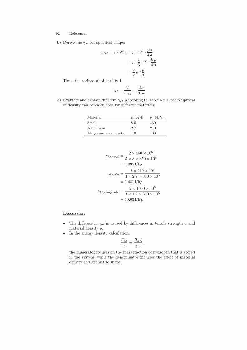
92 References
b) Derive the γht for spherical shape:
mht = ρ π d2ω = ρ · πd2 ·p d
4 σ
= ρ ·1
6π d3 ·
6 p
4 σ
=3
2ρV
p
σ
Thus, the reciprocal of density is
γht =V
mht=
2 σ
3 ρp
c) Evaluate and explain different γht According to Table 6.2.1, the reciprocalof density can be calculated for different materials:
Material ρ [kg/l] σ [MPa]
Steel 8.0 460
Aluminum 2.7 210
Magnesium-composite 1.9 1000
γht,steel =2× 460× 106
3× 8× 350× 105
= 1.095 l/kg.
γht,alu =2× 210× 106
3× 2.7× 350× 105
= 1.481 l/kg.
γht,composite =2× 1000× 106
3× 1.9× 350× 105
= 10.03 l/kg.
Discussion
• The differece in γht is caused by differences in tensile strength σ andmaterial density ρ.
• In the energy density calculation,
Eht
Vht=
Hh ξ
γht.
the numerator focuses on the mass fraction of hydrogen that is storedin the system, while the denominator includes the effect of materialdensity and geometric shape.
References 93
• As a further step in the future, increasing pressurized level (to-wards 700bar), or choosing material with higher tensile strength (till6000MPa) can improve the storage system and will be gradually in-troduced.
Problem 6.6
Evaluate the storage pressure and the specific strength (ratio of tensilestrength to density) of the tank material that would be necessary to meetthe 2015 DOE targets of Table 6.2.1 with gaseous hydrogen.
• Solution
a) Calculate the 2015 DOE target⎧⎪⎨
⎪⎩
Eht
mht= 3.0 kWh /kg
Eht
Vht= 2.7 kWh /l
ξht = 9.0%
(10.30)
b) Calculate the pressurized level
ρh = Eht
Vht·Hh= 2.7×103×3.6×106
120×106 = 81kg/m3
V = Mh
ρh= 2×10⁻³
81 = 2.469× 10⁻⁵m3/mol(10.31)
Solving the RK-equation from Problem 6.1,
p =8.314× 300
V − 1.837× 10⁻⁵−
9.251× 10⁻⁵
√300× V (V + 1.837× 10−5
= 394.6MPa.
c) Calculate tensile specific length of materialDensity reciprocal:
γht =Hl ξht(Eht
Vht
)
=33.33kWh/kg× 0.09
2.7kWh/l
= 1.111l/kg.
Therefore, the tensile specific length is:(σ
ρ
)=
3
2γhtp|p≈395MPa
=3
2× 1.111× 10−3 × 395× 106
= 657.1kNm/kg.
94 References
which is larger than that of magnesium-based composite fiber:
(σ
ρ
)
compsite
=1000
1.9= 526.3kNm/kg
Discussion
• As for current technology level, both the pressurized level and thehousing material tensile strength have to be improved a lot to meetthe 2015 DOE requirement.
• Carbon fiber can probably have a specific tensile strength of a fewthousands kNm/kg, which might be a probably candidate.
Problem 6.7
Explain the explicitness of the number of cells N in (6.72).
• Solution
Assume the first approximation in (6.72) holds:
Paux(t) = P0 +N · κaux · Ifc(t)
According to the semi-empirical data, which sugests a linear dependencybetween Paux and Pst for first order approximation:
Paux ∝ Pst
Paux = C0 + C1 · Pst
= C0 + C1 · Ufc(t) · Ifc(t) ·N.
As the main component of the auxiliary poewr, Pst contains the numberof cell explicitly.
Problem 6.8
For the fuel cell stack of Fig. 6.11, find (i) the maximum output powerPfcs,max, (ii) the current Ifc,P at which this power is yielded, and (iii) thecurrent Ifc,η that maximizes the overall efficiency. Compare the result withthe curves shown in the figure.
• Solution
Assume: According to the fuel cell power & efficiency graph: N =250, urev = 1.23V, uOC = 0.82V , Afc = 200 cm2, Rfc = 0.0024Ω, P0 =100W κaux = 0.05V
References 95
a) Find the optimal current Ifc,PAs is known from (6.79), cell power can be described as:
Pfcs = (N · Uoc −N · κaux) Ifc − P0 −N ·Rfc Ifc2(t)
At optimum, set derivative ∂Pfcs
∂Ifc|Ifc,P
= 0, we have:
N · Uoc −N · κaux = 2N Rfc Ifc,P (t)
Ifc,P = I∗fc =N Uoc −N κaux
2N Rfc
=0.82− 0.05V
2× 0.024Ω= 160.4 A
b) Find the maximum power of one single cell
Pfcs = (N · Uoc −N · κaux) Ifc − P0 −N · Rfc Ifc2(t)
= 250× (0.82− 0.05)× 160.4− 100− 250× 0.0024× 160.42
= 15.34kW
c) Find the optimal current in terms of maximum efficiencyThe cell efficiency can be described as:
ηst(Ifc) = ηidUoc
Urev
(1−
Rfc
IfcUoc −
P0
Uoc Ifc N−κauxUoc
)
As for the same reason, the maximum efficiency is achieved if the deriva-tive is set to zero. ∂ηst
∂Ifc|Ifc,η
= 0givesI2fc,η = P0N Rfc
Thus, the optimal
current in terms of maximum efficiency is:
Ifc,η =
√P0
N Rfc=
√100
250× 0.0024= 12.91A
Problem 6.9
Calculate the same quantities as in Problem 6.8 for a small fuel cell stackpowering a racing FCHEV (see Sect. 8.6). Use the quadratic expression (6.71)for Paux and the following data: N · Uoc = 16.8, N ·Rfc = 0.137, P0 = 19.89,κ1 = 6.6, κ2 = −0.024.
• Solution
Assume: New data and new representation of Pst:
Paux = P0 + κ1 · Ifc(t) + κ2 · Ifc(t).
96 References
where N · Uoc = 16.8, N ·Rfc = 0.137,P0 = 19.89,κ1 = 6.6,κ2 = −0.024.
a) Find the optimal current Ifc,PAs is known from (6.79), cell power can be described as:
Pfcs = (N · Uoc − κ1) Ifc − P0 − (N · Rfc + κ2)I2fc
At optimum, set derivative ∂Pfcs
∂Ifc|Ifc,P
= 0, we have:
Ifc,P = I∗fcN · Uoc − κ1
2 · (N · Rfc + κ2)
=16.8− 6.6
2 (0.137− 0.024)
= 45.13 A
b) Find the maximum power of one single cell
Pfcs = (N · Uoc − κ1) Ifc − P0 − (N ·Rfc + κ2)I2fc
= (16.8− 6.6)× 45.13− 19.89− [0.137 + (−0.024)]× 45.132
= 210.3W
c) Find the optimal current in terms of maximum efficiencyThe cell efficiency can be described as:
ηst(Ifc) =Pfcs(Ifc)
N · Uid · Ifc
= ηidUoc
Urev
(
1−P0 + κ1 Ifc + κ2 I2fc
Uoc Ifc N−
RfcI2fcUoc Ifc
)
As for the same reason, the maximum efficiency is achieved if the deriva-tive is set to zero. ∂ηst
∂Ifc|Ifc,η
= 0givesI2fc,η = P0κ2+N Rfc
Thus, the optimal
current in terms of maximum efficiency is:
Ifc,η =
√P0
κ2 +N Rfc=
√19.89
0.1370.024= 13.25A
Reformers
Problem 6.10
Derive (6.95).
• Solution
References 97
As for a Methanol Reformer, the chemical reactions can be concluded asfollows:
CH3OH +H2O → CO2 + 3H2,∆hR = 58.4kJ/mol
Assume nm, ns, nCO2 , nH2 denotes the number of moles of methanol,water, carbon-dioxide and hydrogen at time t, respectively.
a) MethanolUsing the extent of reaction:
x =nm(0)− nm(t)
nm(0),
we have:nm = nm(0) (1− x).
b) Watersteam
ns = ns(0)− (nm(0)− nm(t))
= ns(0)− nm(0) · x= nm(0)(σ − x)
where σ denotes the ratio of the moles of water to the moles of methanol,which is the feed-in gas ratio and is assumed to be known at the beginningof reaction.
c) Hydrogen
nh = 3 · x · nm(0).
d) Carbon-dioxide
n+ CO2 = 1 · x · nm(0).
e) Derivation of the methanol evolutionSubstitutes all the molar number into the molar fraction, we have:
Cm(x) =nm
nm + ns + nh + nCO2
=nm(0)(1− x)
nm(0)(1− x) + nm(0)(σ − x) + 4 · x · nm(0)
=1− x
(1 + σ) + 2 x
Given that at the beginning of the reforming process, the feed-in gas ratiois predefined ns(0)
nm(0) = σ. Thus,
Cm(0) =nm(0)
nm(0) + ns(0)=
1
1 + σ
Cm(x) = (1 + σ)1− x
1 + σ + 2 · xCm(0).
98 References
which exactly gives (6.95).
Supervisory Control Algorithms
Driver’s Intepretation
Problem 7.1
An ICE-based powertrain has the following characteristics: γ = 15.0, 8.1, 5.3, 3.9, 3.1, 2.6,wheel radius rw = 0.32m, rated engine power Pe,max = 92kW at a speedωe,max = 524 rad/s, engine braking torque Te,min = 20Nm. Build a driver’sinterpretation map. Then, follow a torque control structure to generate anengine torque setpoint for a driver pedal request of 50% at a vehicle speed of100km/h and fourth gear.
• Solution
The curve describing the maximum force available at the wheels consists ofa first part that reproduces the engine maximum torque curve (not known inthis exercise) for the 1st gear, and a second part that is the envelop of themaximum-power engine points at different gears. The maximum-power enginepoint is at ωe = 524 rad/s and Te = 92 · 103/524 = 176Nm.
The vehicle speed at gear i is related to the engine speed by the equationvi = rw/γi · ωe, for i = 1, . . . , 6. The force at the wheels is Ft,i = γi/rw · Te.Since v = 100/3.6 = 27.8m/s is greater than v1 = 524 · 0.32/15 = 11.2m/s,the maximum-power range is active. Therefore, Ft = 92 · 103/V correspondsto 100% accelerator pedal. The maximum brake power is calculated from theengine data as 20 · 524 = 10.5kW. Thus Ft = 10.5 · 103/V corresponds to0% accelerator pedal. At the current speed, the maximum force is 3312N,the minimum force is 378N. For a pedal depression of 50%, assuming linearinterpolation, we have a force request Ft = −378+(3312+378) ·0.5 = 1467N.Assuming 4th gear, the engine torque is Te = 0.32/3.9 · 1467 = 120Nm at aspeed ωe = 27.8 · 3.9/0.32 = 339 rad/s = 3235 rpm.
Problem 7.2
Add an electric machine to the powertrain of Problem 7.1, having thefollowing characteristics: maximum torque Tm,max = 140Nm, base speedωb = 300 rad/s, maximum power Pm,max = 42kW. Calculate the total torquedemand for the same driving situation as in Problem 7.1 if power assist isauthorized at each vehicle speed. Assume coupled regenerative braking.
• Solution

References 99
The vehicle speed corresponding to the base speed of the motor is 300 ·0.32/11 = 8.7m/s = 31.4 km/h, thus lower than v1 (see Problem 7.1). There-fore, the actual vehicle speed corresponds to the maximum-power range of themotor. Summing the two powers yields 92+42 = 134kW. The minimum forceat the wheels does not change with respect to the ICE case. The maximumforce is now Ft = 134 · 103/27.8 = 4820N. For a 50% pedal position, the forcedemand is Ft = −378 + (4820 + 378) · 0.5 = 2221N, which corresponds toa total powertrain torque of Tt = 2221 · 0.32 = 711N. In the 4th gear, thatwould correspond to an engine torque Te = 711/3.9 = 182Nm, which is veryclose to its maximum torque.
Problem 7.3
Propose a driver’s interpretation function for a BEV whose motor and batteryhave the same data as in Problem 4.9. Assume a coupled braking circuit.Calculate the torque setpoint for (i) ωm = 0 rad/s and 0% pedal depression,(ii) ωm = 100 rad/s and 0% pedal depression, (iii) ωm = 250 rad/s and 50%pedal depression.
• Solution
The 0% pedal position corresponds to the minimum between Ia,min as calcu-lated in Problem 4.35 and a negative torque for which the driver has a similarfeeling than with an ICE-based powertrain. Fix this torque to, say, 1/10 ofthe maximum torque. Thus
Ia,min =
⎧⎪⎪⎪⎪⎪⎨
⎪⎪⎪⎪⎪⎩
−κa ·ωm
2 · Rafor ωm <
2 · Ra · (0.1 · Imax)
κa,
−0.1 · Imax for ωm <Pmax
κa · 0.1 · Imax,
−Pmax
κa · ωmelse.
while for 100% acceleration
Ia,max =
⎧⎪⎨
⎪⎩
Imax for ωm <Pmax
κa · Imax,
Pmax
κa · ωmelse.
The curve Ia = f(α,ωm) is obtained by interpolation between these two limits,Ia = Ia,min + α · (Ia,max − Ia,min).
For the case (i), Ia,min = 0 and Ia = Tm = 0.
For the case (ii), ωm = 100 rad/s and ωm > 2·Ra·(0.1·Imax)κa
= 2 · 0.05 · (0.1 ·88)/0.25 = 3.52 rad/s. Thus Ia = Ia,min = −0.1·88 = −8.8A, Tm = −2.2Nm.
For the case (iii), ωm = 250 rad/s and ωm < 4 · 103/(0.25 · 0.1 · 88) =1818 rad/s. Thus Tm = −2.2 + 0.5 · (22 + 2.2) = 9.9Nm.
100 References
Problem 7.4
Derive a PI model for a human driver of an electric vehicle that tries tofollow a prescribed drive cycle acting on the acceleration pedal. Derive a gain-scheduling tuning of the PI parameters. Vehicle data: mass mv = 1360kg,12 ·ρa ·Af · cd = 0.25N/(m/s)2. Evaluate the PI coefficients for a vehicle speedof 20m/s. Assume perfect recuperation (decoupled braking).
• Solution
Vehicle dynamics can be generally written as
dv
dt=
Ft − c0 − c2 · v2
mv
The driver is sensitive to the difference between v(t) and vs(t). Its action ison the acceleration and brake pedals. Define the general driver’s output asthe force Ft (positive for traction, negative for braking). Thus
dv
dt=
u− c0 − c2 · v2
mv,
u = Kp · (v − vs) +Ki ·∫(v − vs) dt.
Linearize around an operating point vs, then define us = c0+c2 ·v2s , z = v−vs,w = u− us. Then evaluate
dz
dt=
w − c2 · (v2 − v2s)
mv≈
w − c2 · 2 · vs · (v − vs)
mv=
w − 2 · c2 · vs · zmv
= K·w−a·z,
where K = 1/mv and a = 2 · c2 · vs/mv.Now close the loop with the driver regulator
w = Kp · z +Ki ·∫
z dt
Obtain
s2 ·z = K ·Kp ·s ·z+K ·Ki ·z−a ·s ·z → z(s) ·(s2+(a−K ·Kp) ·s−K ·Ki) = 0
By pole-placement, target at
ωn =√(−K ·Ki) = 1 rad/s,
andζ = (a−K ·Kp)/(2 · ωn) = 0.7
With the numerical values, K = 1/1360 = 7.35 · 10−4, a = 2 · 0.25 ·vs/1360 = 3.7 · 10−4 · vs, Ki = −1/K = −1360, Kp = (a − 0.7 · 2)/K =(3.7 · 10−4 · vs − 0.7 · 2)/7.35 · 10−4. For vs = 20m/s obtain Kp = −1898N.
References 101
Regenerative Braking Control
Problem 7.5
Derive an ideal law to split the braking effort between the two axles underthe assumption that the adherence is the same at each wheel.
• Solution
Write force and torque balance equations for a two-wheel equivalent vehicle.We have four equations in the four unknowns N1, N2 (normal forces), F1, andF2 (longitudinal forces), where subscript 1 is for front wheels and subscript 2for rear wheels, while the total required force Ft is known:
F1 + F2 = Ft, (balance of logitudinal forces)
N1 +N2 = N, (balance of normal forces)
N · b = Ft · h+N1 · (a+ b), (balance of momenta)
F1
N1=
F2
N2, (equal adherence)
where N = mv · g is the vehicle weight, a and b are the horizontal distancesof the wheel axles from the center of gravity (CoG), and h the height of theCoG.
By combining these four equations, obtain
N1 =N · ba+ b
−Ft · ha+ b
N2 = N −N1 =N · aa+ b
+Ft · ha+ b
During braking, Ft < 0 and the front weight increases. Moreover, the equaladherence condition reads
F1 ·N2 = F2 ·N1. (10.32)
For a given Ft, obtain the ideal split
F1 ·(N ·a−Ft ·h) = (F −F1) ·(N ·b−Ft ·h) → F1 ·N(a+b) = Ft ·(N ·b−Ft ·h),
or
F1 =Ft · ba+ b
−F 2t · h
N · (a+ b).
In terms of torques
T1 =Tt · ba+ b
−T 2t · h
N · rw · (a+ b),
102 References
T2 =Tt · aa+ b
+T 2t · h
N · rw · (a+ b).
The equal adherence curve T2 = T2(T1) is obtained by manipulating (??)as
F1 · (N · a+ Ft · h) = F2 · (N · b− Ft · h)or
T 21 · h+ 2 · T1 · T2 · h+ T1 ·N · a · rw − T2 ·N · b · rw + T 2
2 · h = 0 (10.33)
Problem 7.6
Consider a vehicle having an electric powertrain on the rear axle, withTm,max = 1540Nm (at the wheels), Pm,max = 42kW, and the followingvehicle characteristics (see Problem 7.5): static weight distribution fractions = 0.40, height of CG h = 55cm, wheelbase l = 2.685m, wheel radiusrw = 0.32m, vehicle mass mv = 1932kg. Evaluate the regenerative brakingtorque and the frictional braking torque on the front and rear axles for a totalbraking torque Tt = −1200Nm, vehicle speed v = 90km/h, under (i) a max-imum regeneration strategy, (ii) a constant braking distribution between theaxles of 70%–30%, (iii) ideal braking as in the result of Problem 7.5, and (iv)a modified brake pedal that induces regenerative braking up to a decelerationof 0.05 g and then frictional braking with a constant braking distribution of70%–30%.
• Solution
At v = 90km/h the maximum regenerative capability of the electric power-train is
42 · 103v3.6 · 1
0.32
= 537Nm.
The braking power is90 · 4003.6 · 0.32
= 31.2 kW.
In the case (i), Trec = −537Nm; T1 = −1200 + 537 = −663Nm, T2 =0Nm. The braking split ratio is 55%/45%. However, this value is above theequal-adherence curve, thus it is not admissible. The quantity Trec should belimited as in the case (iii).
In the case (ii), Trec = −0.30 · 1200 = −360Nm, T1 = −1200 + 360 =−840Nm, T2 = 0Nm.
In the case (iii), using the formula of Problem 7.5,
Trec = 0.40 · (−1200) +12002 · 0.55
1932 · 9.81 · 0.32 · 2.685= −431Nm,
and T1 = −1200+431 = −769Nm, T2 = 0Nm (braking split ratio 64%/36%).In the case (iv), the threshold torque is mv · a · rw = 1932 · (−0.05) · 9.81 ·
0.32 = −300Nm. Thus Trec = −300Nm, T1 = 0.7 ·(−1200+300) = −630Nm,T2 = −270Nm.
References 103
Problem 7.7
Consider a conventional (coupled) braking system where T2 = k · T1 (T1 <0, T2 < 0). Calculate the maximum value of the adherence that can be ob-tained under the assumption of equal adherence between the axles (ideal dis-tribution curve) and the corresponding total braking torque. Check what hap-pens for higher braking torques. Then, calculate the limit value of k that canbe achieved. Use the numerical values of Problem 7.6.
• Solution
The limit of conventional braking systems occurs when the practical brakingsplit curve meets the ideal split curve. The latter is given by (??), while theformer reads T2 = k · T1. By combining these two equations, obtain
T1 =−N · rw · (a− k · b)
h · (1 + k)2
and
T2 =−k ·N · rw · (a− k · b)
h · (1 + k)2.
Since both T1 and T2 are negative quantities, a condition on k is thata− k · b) > 0, or
k <a
b.
For k = a/b, the braking distribution is such that
T1
Tt=
1
1 + k,
T2
Tt=
k
1 + k.
The common value of the adherence factor (µ1 = µ2 = µ) is obtained bycalculating N1 and N2. First evaluate
Tt = T1 + T2 = (1 + k) · T1 =−N · rw · (a− k · b)
h · (1 + k).
Then, find
N1 =N · b− Tt · h · rw
a+ b=
N · b+N · (a · k − b)
(1 + k) · (a+ b), N2 =
N · k1 + k
and the adherence factor as
µ =−T1
N1 · rw=
−T2
N2 · rw=
a− k · bh · (1 + k)
.
With the data of Problem 7.6, the limit k = 0.4/0.6 = 0.667. For a valuek = 0.3/0.7 = 0.429, the maximum adherence is 0.488. The limit values
104 References
of T1 and T2 are -2055Nm and -881Nm. The maximum braking torque isTt = −2935Nm.
For higher braking torques, e.g., Tt−3500Nm, the braking split ratio wouldbe 2450/1050Nm. The vertical forces would be N1 = 1932·9.81
1+0.429 = 13632N,N2 = 1932 · 9.81 − 13632 = 5321N. Thus µ1 = 2450/13632/0.32 = 0.56while µ2 = 1050/0.32/5321 = 0.62. This circumstance µ2 > µ1 is potentiallydangerous and should be avoided.
Problem 7.8
Derive the ideal braking distribution law as in Problem 7.5 when one axle inmotoring while the other is braking (for instance, battery recharge mode inan HEV with an engine on the front axle and an electric machine on the rearaxle). For simplicity, assume a = b.
• Solution
As in Problem 7.5,
F1 + F2 = Ft, (balance of logitudinal forces)
N1 +N2 = N, (balance of normal forces)
N · b = Ft · h+N1 · (a+ b), (balance of momenta)
but nowF1
N1= −
F2
N2,
the latter being the condition of equal adherence µ1 = −µ2. By combiningthese four equations, obtain
N1 =N · ba+ b
−Ft · ha+ b
N2 = N −N1 =N · aa+ b
+Ft · ha+ b
F1 ·N2 = −F2 ·N1, (10.34)
from whence
F1·(N ·a+F1·h+F2·h) = −F2·(N ·b−F1·h−F2·h) → F1·N ·a+h·F 21 = −N ·b·F2+h·F 2
2 .
There are two solutions to this equation for a = b. One is F2 = F1 + N ·ah . The
other is F2 = −F1, which does not imply the satisfaction of the total force Ft
but constitutes a limit in the 2nd and 4th quadrant of the plane F1—F2.From the first solution, find
T1 =Tt
2−
N · a · rw2 · h
, T2 =Tt
2+
N · a · rw2 · h
.
References 105
Dynamic Coordination
Problem 7.9
In a series HEV the supervisory control yields engine torque and speed set-points Te and ωe. Derive a simple generator controller in order to achieve thedesired speed of the APU.
• Solution
The dynamics of the APU can be described by the simplified equation
Θapu ·dωe(t)
dt= Te(t)− Tg(t).
The generator torque open-loop setpoint is Tg,sp = Te,sp. However, in order tolet the generator speed converge toward the value ωe, at least a proportionalcorrection should be added. Assuming Te(t) = Te,sp(t),
Tg(t) = Te(t) + kp · (ωg(t)− ωe(t)).
The closed-loop dynamics therefore reads
Θapu · s · ω = −Kp · ω,
which converges to ω = 0 with a time constant Θapu/kp.
Problem 7.10
Derive the dynamic equations to control the generator torque in a simple PSD-based system like that of the Toyota Prius. Neglect the generator inertia.
• Solution
Manipulate the dynamic equations (4.163)–(4.164) with Θsun = 0 to obtain
Θcarrier ·dωe(t)
dt= Te(t)−
1 + z
z· Tg(t),
Θring ·dωf (t)
dt=
1
z· Tg(t) + Tm(t)− Tf(t).
where Θcarrier is represented by Θe and Θring by the vehicle inertia.The resulting dynamics for the engine speed is rather similar to that of
Problem 7.9, except for the 1+zz factor now multiplying the generator torque.
It is laborious but straightforward to show that the same dynamic equationfor ωe (but not for ωf !) applies also to the case where Θsun is not negligible.
106 References
Problem 7.11
In a post-transmission parallel HEV, in principle it is possible to compensatethe torque gap at the wheels during a gear shift. Evaluate the time elapse afterwhich the vehicle speed before the shift is recovered (tr, recovery time) andthe necessary electric energy for a downshift from 4th to 3rd gear occurringduring a constant vehicle acceleration. Data: gear ratios including final gearγ = 5, 4, motor gear ratio = γm = 11, transmission efficiency ηt = 0.97,motor efficiency ηm = 0.85, wheel radius rw = 0.29m, engine shift speedωe = 4500 rpm, shift duration ts = 1 s; acceleration a = 0.5m/s2, vehiclemass mv = 1360kg, cr = 0.009, cd · Af = 0.5m2.
• Solution
Define the two time points t1 and t2 as the beginning and the end of the gearshift (t2 − t1 = ts). Evaluate
v1 # v(t1) =ωe,shift
γ3
rw
=4500·π
305
0.29
= 27m/s = 98 km/h.
Without compensation, the vehicle speed decreases during the shift accordingto the law
dv(t)
dt= −g · cr −
ρa ·Af · cd · v2
2 ·mv,
or (2.17) with α =√
0.5·1.21360·0.5 = 0.015, β =
√9.8 · 0.009 = 0.3. The coasting
velocity at t2 is
v2 =β
α· tan
(arctan
(α
β· v1)− α · β · (t2 − t1)
)
=0.3
0.015· tan
(arctan
(0.015
0.3· 27)− 0.015 · 0.3 · 1
)
= 26.7m/s = 96 km/h.
After the engine is engaged again, the speed increases according to the linearlaw v(t) = v2 + a · t. The recovery time is
t3 =v1 − v2
a=
0.3
0.5= 0.6 s.
Thus the total time lost is tr = ts + t3 = 1 + 0.6 = 1.6 s.This time can be recuperated if the motor provides the missing torque
during the shift. This torque is
Tm(t) =Ft(t)γm
rw
=mv · a+mv · cr + ρa · cd ·Af · v(t)2
2 · γm
rw
.
The energy provided by the motor is calculated from
References 107
∆Em =
∫ωm(t) · Tm(t)dt =
1
ηt·∫
Ft(t) · v(t)dt =
=1
ηt·((mv · a+mv · cr) ·
∫v(t)dt+
∫0.5 · ρa · cd · Af · v(t)3dt
)
=1
ηt· (mv ·
v22 − v212
+mv · cr2 · a
· (v22 − v21) + 1.2 · cd · Af · (v42 − v41)/(8 · a)),
where now v2 = v1 + a · ts = 27 + 0.5 · 1 = 27.5m/s. Thus the energy is
∆Em =1
0.97·(1360 ·
27.52 − 272
2+
1360 · 0.0092 · 0.5
· (27.52 − 272)+
+0.5 · 1.2 · 0.5 ·27.54 − 274
4 · 0.5
)= 25.7 kJ,
with an average power Pm = 25.7kW.
Problem 7.12
Consider a parallel HEV with an electric machine mounted on the primaryshaft of the gearbox with a reduction gear ratio γm. During a gear shift, theinertia of the motor sums up to the inertia of the primary shaft. To reduce thesynchronization lag, the motor in principle could yield a torque to compensateits own inertia. Model this situation with simple equations. Then calculate themotor energy consumption for the following data: γm = 3.3, downshift from4th to 3rd gear with γ3 = 5.5, γ4 = 3.9, vehicle speed v = 60km/h, motorinertia Θm = 0.07 kg/m2.
• Solution
During synchronization without motor assist, the dynamics of the primaryshaft reads
Θp ·dωp(t)
dt= Tm,i(t) · γm + k ·
(v(t) · γ3
rw− ωp(t)
),
where the second right-hand term simulates the action of the synchronizerwhich is proportional to the difference between the secondary speed with thenew gear ratio and the primary speed. The term Tm,i is transmitted from themotor inertia
Tm,i = −Θm ·dωm
dt.
Since ωm = γm · ωp,
(Θp + γ2m ·Θm) ·dωp(t)
dt= k ·
(v(t) · γ3
rw− ωp(t)
)
and the primary shaft speed increases from the initial value ωp,4 = γ4·vrw
up tothe new value ωp,3 = v·γ3
rw. The variation law is (ideally) asymptotic,
108 References
ωp(t) =γ3 · v(t)
rw+
(γ4 · v(t)
rw−γ3 · v(t)
rw
)· exp
(−k · tΘ
),
where Θ # Θp + Θm · γ2m. To decrease the motor inertia, one should apply atorque Tm such that
Θm ·dωm(t)
dt= Tm − Tm,i
such that Tm,i = 0, thus
Tm = Θm ·dωm(t)
dt= Θm · γm ·
dωp(t)
dt
=Θm · γm · k ·
(v(t) · γ4
rw− ωp(t)
)
Θp,
where ωp(t) is still calculated with the equation above but with Θp instead ofΘ.
The motor power is
Pm = Tm · ωm =
= Θm · γm ·dωp
dt· γm · ωp = Θm · γ2m · ωp ·
dωp
dt.
The energy consumed results from the integral of Pm or
Em = Θm · γ2m ·ω2p,3 − ω2
p,4
2.
Numerically,
ωp,3 =70 · 5.53.6 · 0.32
= 334 rad/s
ωp,4 =70 · 3.93.6 · 0.32
= 237 rad/s
Em = 0.07 · 3.32 ·3342 − 2372
2= 21 kJ
Heuristic Energy Management Strategies
Problem 7.13
Consider a pre-transmission, single-shaft parallel HEV with fixed gear reduc-tion. System data: gear ratio including final gear ratio γ = 4, engine maximumtorque curve Te,max(ωe) = 50+0.7 ·ωe− 1 · 10−3 ·ω2
e , motor maximum torqueTm,max = 150Nm, motor maximum power Pm,max = 25kW, vehicle datacD = 0.33, Af = 2.5m2, cr = 0.013, mv = 1500kg, Θw = 0.25kgm2, rw =0.25m. Consider the simple, SOC-independent heuristic energy-managementstrategy:
References 109
• EV mode if ωe < 1000 rpm or if Te < 40Nm,• power assist mode if Te > Te,max,• else, recharge mode if Te > 0• regenerative braking if Te < 0.
Evaluate the scheduled mode, the engine torque, and the motor torque forthe following driving situations: (i) v = 17km/h, a = 1.37m/s2; (ii) v =38.76km/h, a = 0.094m/s2; (iii) v = 28.8km/h, a = 1.56m/s2; (iv) v =95km/h, a = 0.19m/s2.
• Solution
For the case (i) the required propulsion force is
Ft = (mv +Θw
r2w · γ2) · a+mv · 9.81 · cr +
1
2· ρa · cD · Af · v2 =
= 1503 · 1.369 + 191.3 + 0.47 · 4.752 = 2257N.
The engine torque would be Te = Ft · rwγ = 2257·0.25/4 = 141Nm. The engine
speed would be ωe = v · γrw
= 75.9 rad/s = 725 rpm. The mode selected would
be the ZEV (ωe < 1000 rpm and Te > 0). The base speed is 25 · 103/150 =167 rad/s. The motor torque Tm = 141Nm is lower than the motor maximumtorque at 725 rpm, which is 150Nm.
For the case (ii), the required force is 1503 · 0.094 + 191.3 + 0.47 ·(38.76/3.6)2 = 387Nm. The engine torque would be of 387 ·0.25/4 = 24.2Nm.The engine speed would be 38.76/0.25 · 4 = 172 rad/s = 1645 rpm. The modeselected would be again the ZEV (Te < 40Nm with ωe > 1000 rpm). At1645 rpm (higher than the motor base speed) the motor maximum torque is25 · 103/172 = 145Nm. Thus the ZEV mode is feasible.
For the case (iii), the required force is 1503·1.56+191.3+0.47·(28.8/3.6)2 =2535N. The engine torque would be of 160Nm. The engine speed would be of1230 rpm. The engine max torque at that speed would be Te,max = 50+ 0.7 ·128 − 1 · 10−3 · 1282 = 123Nm. Thus the mode selected would be the boost(Te > Te,max and ωe > 1000 rpm). The motor torque would be 160 − 123 =37Nm, which is lower than the motor max torque.
For the case (iv), the required force is 805N. The engine torque would beof 50Nm. The engine speed would be 4033 rpm = 422 rad/s. Thus the selectedmode would be the battery recharge (Te > 40Nm and ωe > 1000 rpm). Themaximum generating torque at 422 rad/s is −25 · 103/422 = −59Nm. Thusthe maximum engine torque could be 50+ 59 = 119Nm (feasible because themaximum engine torque is 167Nm).
Problem 7.14
Consider the following SOC-dependent energy-management heuristic strat-egy:
110 References
• engine on with Pe = Pt − Pt,b(ξ) if Pt > Pe,start(ξ),• else, engine off,
with the definitions Pt,b = −Pm,max+2·Pm,max/(ξhi−ξlo)·(ξ−ξlo), Pe,start =Pm,max/(ξhi − ξlo) · (ξ − ξlo) and the numerical values ξhi = 80%, ξlo = 40%.Assume a unit-efficiency motor operation. Perform again the calculations ofProblem 7.13, for ξ = 55, 70%.
• Solution
For the case (ii), engine possible speed and torque ωe = 172 rad/s, Te =24.2Nm would lead to Pe = 4.16 kW. Since Pm,max = 25kW, Pe,max =24.2kW, evaluate
Pe,start =ξ − 40
80− 40· Pm,max = 9.4 kW for ξ = 55%,
= 18.75 kW for ξ = 70%.
Now, Pe < Pe,start, thus the selected mode is ZEV.For the case (iii), ωe = 129 rad/s, Te = 160Nm would lead to Pe =
20.6kW. In this case Pm,max = 150 · 129 = 19.3 kW, Pe,max = 15.95kW, thusPe,start = 7.2, 14.5 kW for the two SOC values. In both cases, Pe > Pe,start.Evaluate Pt,b = −19.3 + (ξ − 40)/40 · (19.3 · 2) = −4.8; 9.7kW. Therefore,Pe would be 25.4; 10.9kW. After saturation, Pe = 15.95; 10.9 and obtainas a difference Pm = 4.65; 9.7 (boost mode).
Fot the case (iv), ωe = 422 rad/s, Te = 50Nm would lead to Pe =21kW. Since Pm,max = 25kW and Pe,max = 70.6kW, evaluate Pe,start =9.4; 18.75kW. In both cases, Pe > Pe,start. Evaluate Pt,b = −0.55; 18.2kWand find Pe = 21.55; 2.8kW. No saturation is needed and Pm = −0.55, 18.2thus the selected mode is recharge, resp., boost.
Problem 7.15
Give an intepretation of the heuristic energy-management strategy of Prob-lem 7.14 in terms of equivalent “cost” of the battery power with respect to thefuel power. Assume a Willans-type engine model with constant parameters eand P0 and a unit-efficiency electric machine.
• Solution
The heuristic rule reads (Pt is the demand power)
Pe = 0 if Pt > Pe,start + Pt,b
Pe = Pt − Pt,b if Pt > Pe,start + Pt,b.
Define an “equivalent” power consumption as H = Pe + s ·Pm, where s is theequivalence factor. Using a Willans engine model,
References 111
H =P0
e· (Pmt > 0) +
Pe
e+ s · (Pt − Pe).
Note that:
• For Pe = 0, H = s · Pt.• For Pe = Pt − Pt,b, H = P0
e + Pt−Pt,b
e + s · Pt,b.
The switching condition for which Pe = 0 is preferable is that s · Pt <P0e +Pt−Pt,b
e +s·Pt,b, that is, Pt·(s− 1
e
)< P0
e +Pt,b·(s− 1
e
), or Pt <
P0e·s−1+Pt,b.
By comparing this switching condition with the heuristic rule, derivePe,start as
Pe,start =P0
e · s− 1+ Pt,b,
from whence derive
s · e =1 + P0
Pe,start − Pt,b
as the equivalence rule between the two strategies (i.e., between s and Pe,start).
Optimal Energy Management Strategies
Problem 7.16
Derive the exact formulation of the Euler-Lagrange equation (7.14) if theequivalent-circuit parameters of the battery are affine functions of SoC asdescribed by (4.64) and (4.66). Consider the following system and operatingpoint: battery capacity Qb = 6.5Ah, nominal open-circuit voltage Uoc =250V, nominal internal resistance Ri = 0.3Ω, electric power Pb = 15kW,variation of the open-circuit voltage with respect to SOC κ2 = 20V, andvariation of the internal resistance κ4 = −0.1Ω. Evaluate the characteristictime constant associated with the variation of the Lagrange multiplier andassess the constant-µ approximation.
• Solution
The Hamiltonian function is
H =∗mf +µ · x,
where x = −Ib/Q0. The Euler–Lagrange equation is written as
µ = −∂H
∂x=
µ
Q0·∂Ib∂x
For an equivalent circuit model,
112 References
Ib =Uoc
2 · Ri−
√U2oc
4 ·R2i
−Pb
Ri#
Uoc
2 ·Ri−A
∂Ib∂Uoc
=1
2 · Ri−
1
2 ·A·
Uoc
2 · R2i
∂Ib∂Ri
= −Uoc
2 ·R2i
−1
2 ·A·(−
U2oc
2 ·R3i
+Pb
R2i
)
Numerically,
A =
√2502
(2 · 0.3)2−
15 · 1030.3
= 351.58 A
∂Ib∂Uoc
=1
2 · 0.3−
1
2 · 351.58·
250
2 · 0.32= −0.31 A/V
∂Ib∂Ri
= −250
2 · 0.32−
1
2 · 351.58·(−
2502
2 · 0.33+
15 · 103
0.32
)= 20 A/Ω
∂Ib∂x
=∂Ib∂Uoc
·∂Uoc
∂x+∂Ib∂Ri
·∂Ri
∂x= −0.31 · 20 + 20 · (−0.1) = −8.2 A/-
and finally obtain
µ
µ=∂Ib∂x
·1
Q0= −
8.1
6.5 · 3600= −
1
2854 s.
Problem 4.36
Starting from the results of Problems 7.16, 4.26, find an approximated ex-pression for the variation of the Lagrange multiplier. Evaluate the error withrespect to the exact solution.
• Solution
Using the result of Problem 4.26,
Ib ≈ I =Pb
Uoc+ 2 ·
Ri
U3oc
· P 2b ,
thus
∂I
∂Uoc= −
Pb
U2oc
− 6 ·Ri
U4oc
· P 2b
∂I
∂Ri=
2
U3oc
· P 2b
With the numerical values of Problem 7.16 compared to the exact solution,
References 113
∂I
∂Uoc= −
15 · 103
2502− 6 ·
0.3
2504·(15 · 103
)2= −0.34 A/V (10% error)
∂I
∂Ri=
2
2503·(15 · 103
)2= 28.8 A/Ω (50% error)
∂I
∂x= −0.34 · 20 + 29 · (−0.1) = −9.7 A (20% error)
Problem 7.18
At low temperature operation, the variation of the internal parameters of abattery can be significant. Develop a version of the ECMS where variationsof internal resistance, via the parameter κ3 of (4.66), with temperature areaccounted for. Cell data: κ1 = 3.4V, κ2 = 0.5V, κ4 = 0, and
κ3 = 0.015− ϑb ·0.01
40,
with ϑb in C. The nominal SOC is ξ = 0.5, temperature ϑ = 25 C, powerPb = 0.1 · Pb,max, thermal capacitance Ct,b = 300 J/K, thermal conductance1/Rth = 0.5W/K, and capacity Qb = 6Ah. Evaluate the time constant of theadjoint states.
• Solution
The quantity to be minimized is still the fuel consumption rate. The SOCvariation is still proportional to the current. However the latter varies as afunction of SOC and temperature. Thus the state equation for the temperaturemust be taken into account. The Hamiltonian is
H =∗mf +µ ·
∂ξ
∂t+ ν ·
∂ϑ
∂t,
where ∂ξ/∂t = −Ib/Q0 and
∂ϑ
∂t=∂ϑ
∂t=(Ri · I2b − α · ϑ
)·
1
Ct,b,
where ϑ # ϑ− ϑamb. The Euler–Lagrange equations read
µ = −∂H
∂ξ= µ ·
1
Q0·∂Ib∂ξ
ν = −∂H
∂ϑ= −ν ·
(2 · Ri · Ib ·
∂Ib∂ϑ
− α
)·
1
Ct,b
The quantity ∂Ib/∂ξ is calculated as
∂Ib∂ξ
=∂Ib∂Uoc
·∂Uoc
∂ξ+∂Ib∂Ri
·∂Ri
∂ξ=
∂Ib∂Uoc
· κ2 +∂Ib∂Ri
· κ4
114 References
while∂Ib∂ϑ
=∂
∂Ri·∂Ri
∂ϑ=∂Ib∂Ri
·∂κ3∂ϑ
With the numerical values for the open-circuit voltage and the internal resis-tance are calculated as
Uoc = κ1 + κ2 · q = N · (3.4 + 0.5 · 0.5) = 3.65 ·N V
Ri = κ3 + κ4 · q = N ·(0.015− 0.01 ·
25
40
)= 0.009 ·N Ω,
while the maximum power can be calculated with equation (4.74)
Pb,max =U2oc
4 ·Ri=
3.652 ·N2
4 · 0.09 ·N= 370 ·N W
Pe = 0.1 · Pb,max = 37 ·N W.
This results in the numerical value for the current
A =
√U2oc
4 ·R2i
−Pb
Ri=
√3.652
4 · 0.0092−
37
0.009= 192 A
Ib =Uoc
2 ·Ri−
√(Uoc
2 · Ri
)2
−Pb
Ri=
=3.65
2 · 0.009−
√(3.65
2 · 0.009
)2
−37
0.009= 10.5 A
The variations in the current relative to vriations in the states ξ,ϑ are now
∂Ib∂Uoc
=1
2 · Ri·(1−
Uoc
2 · Ri · A
)=
=1
2 · 0.009 ·N·(1−
3.65
2 · 0.009 · 192
)= −
3.12
NA/V
∂Ib∂Ri
= −Uoc
2 ·R2i
−1
2 ·A·(Pb
R2i
−U2oc
2 ·R3i
)=
= −3.65
2 · 0.0092−
1
2 · 192·(
37
0.0092−
3.652
2 · 0.0093
)=
75.2
NA/Ω
∂Ib∂ξ
= −3.12 · 0.5 + 75.2 · 0 = −1.56 A
∂Ib∂ϑ
= 75.2 ·−0.01
40= −0.019 A/K
Following time constants of the lagrange mutlipliers are obtained
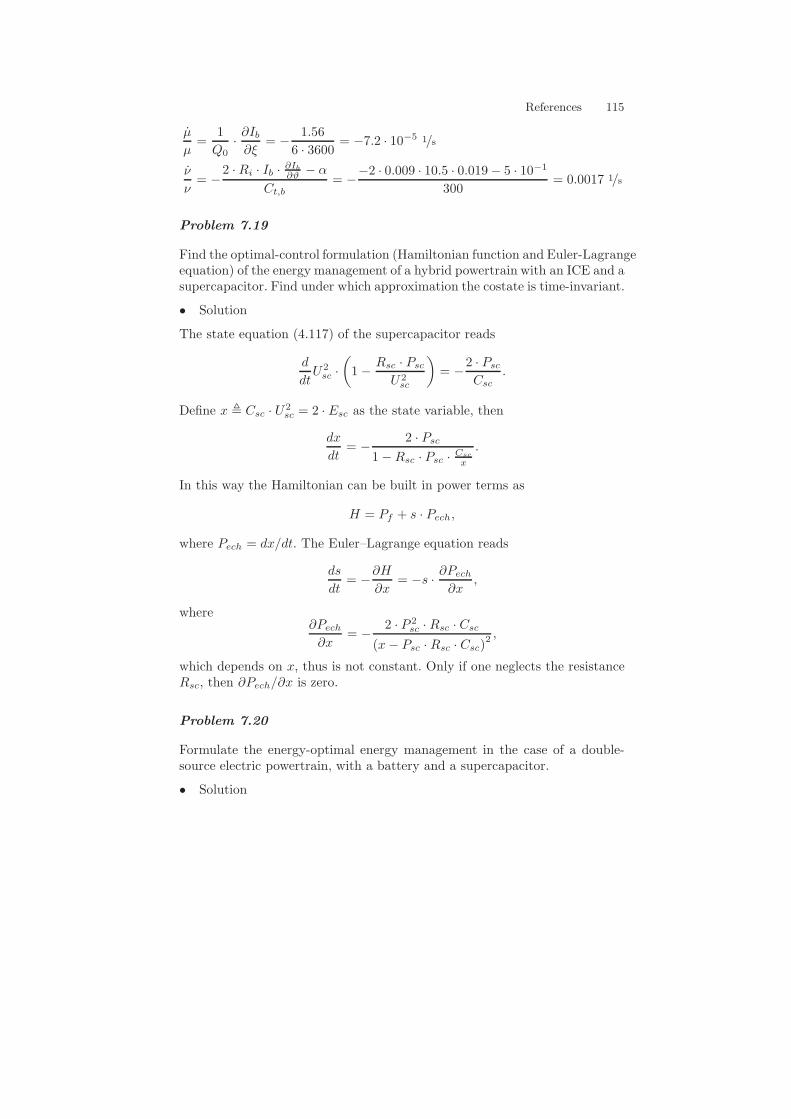
References 115
µ
µ=
1
Q0·∂Ib∂ξ
= −1.56
6 · 3600= −7.2 · 10−5 1/s
ν
ν= −
2 ·Ri · Ib · ∂Ib∂ϑ − α
Ct,b= −
−2 · 0.009 · 10.5 · 0.019− 5 · 10−1
300= 0.0017 1/s
Problem 7.19
Find the optimal-control formulation (Hamiltonian function and Euler-Lagrangeequation) of the energy management of a hybrid powertrain with an ICE and asupercapacitor. Find under which approximation the costate is time-invariant.
• Solution
The state equation (4.117) of the supercapacitor reads
d
dtU2sc ·(1−
Rsc · Psc
U2sc
)= −
2 · Psc
Csc.
Define x # Csc · U2sc = 2 · Esc as the state variable, then
dx
dt= −
2 · Psc
1−Rsc · Psc · Csc
x
.
In this way the Hamiltonian can be built in power terms as
H = Pf + s · Pech,
where Pech = dx/dt. The Euler–Lagrange equation reads
ds
dt= −
∂H
∂x= −s ·
∂Pech
∂x,
where∂Pech
∂x= −
2 · P 2sc · Rsc · Csc
(x− Psc · Rsc · Csc)2 ,
which depends on x, thus is not constant. Only if one neglects the resistanceRsc, then ∂Pech/∂x is zero.
Problem 7.20
Formulate the energy-optimal energy management in the case of a double-source electric powertrain, with a battery and a supercapacitor.
• Solution
116 References
In this case the optimization criterion is the minimization of the battery con-sumption, i.e.,
L = Pech = Uoc · Ib,while the global constraint is over the supercapacitor SOC or voltage,
x(tf ) =1
2· Csc · U2
sc(tf ) = x(0).
Therefore the Hamiltonian reads
H = Uoc · Ib(Pb) + s · Psc,
where Psc =dxdt , and the Euler–Lagrange equation is
ds
dt= −
∂H
∂x= −s
∂Psc
∂x,
for whose development see Problem 7.19. The global constraint over the statex can be used to find the unknown initial value of s. However, the constraintslocally applied to the state x are even more critical in this case.
Problem 7.21
Formulate the optimal energy management for a parallel HEV that includesengine temperature variations. Assume that the cold-engine fuel consumptionis given by an equation of the type
∗mf (Te,ωe,ϑe) =
∗mf,w(Te,ωe) · f(Te,ωe,ϑe),
where ϑe is one engine relevant temperature and∗mf,w is the warm-engine fuel
consumption. Moreover, assume an engine temperature dynamic of the type
Ct,e · ϑe = Pheat(Te,ωe,ϑe)− α · (ϑe − ϑamb) .
• Solution
The cost function is L =∗mf . There exist two state variables, namely, the SOC
of the battery ξ and the engine temperature ϑe. Thus the Hamiltonian is
H =∗mf (Te,ωe,ϑe) + µ ·
dξ
dt+ ν ·
dϑedt
,
where ξ = g(Te, t, ξ) and ϑ is given in the problem text.The Euler–Lagrange equations read
µ = −∂H
∂ξ= −µ ·
∂ξ
∂ξas usual (see Problem 7.16)
ν = −∂H
∂ϑe= −
∂∗mf
∂ϑe− ν ·
∂ϑe∂ϑe
= − ∗mf,w ·
∂f
∂ϑe−
ν
Ct,e·(∂Pheat
∂ϑe− α
)
Define ν = −ν · Ct,e to have a third term in the Hamiltonian that has theunits of a power. In that case, the state variable would be the thermal energyaccumulated Eth. Since there is no constraint over the state ϑe (or Eth), theterminal value of the second Lagrange multiplier ν must be ν(T ) = 0.
References 117
Problem 7.22
Evaluate the optimal gear ratio profile during an ICE-based vehicle accelera-tion from rest to vf on a flat road. Use (i) the acceleration time tf and (ii) thefuel consumption mf as the performance index. Make the following simplify-ing assumptions: constant engine parameters Te = Te,max, e, P0, continuouslyvariable gear ratio, linearized vehicle dynamics
v =Ft
mv− b · v,
where Ft = u · Te and u = γ/rw. Verify the solution given by optimal con-trol theory by analyzing the dependency of the criterion on the gear ratio.Numerical data: b = 10−2, u = γ/rw ∈ [umin, umax] = [2, 12], mv = 1000kg,vf = 100km/h, Te = 150Nm, e = 0.4, P0 = 2kW.
• Solution
Fuel power consumption:
Pf =Te · ωe + P0
e=
Te · u · v + P0
e.
Case (i)
J =
∫ tf
0dt = tf
L = 1
H = 1 + µ ·(u · Te
mv− b · v
)
s =∂H
∂u= µ ·
Te
mv
uo =
umin if s < 0
umax if s > 0
Euler–Lagrange equation:
µ = −∂H
∂v= µ · b,
thusµ(t) = µ(0) · eb·t
Use the condition that H ≡ 0 for “free final time” problems, to find that µ(0)must be negative,
µ(0) = −1
u·Te
mv
,
118 References
since the quantity u · Te/mv is positive. Thus µ(t) is always negative and s(t)is negative as well. Consequently,
uo(t) = umax.
Intuitively, the longest gear is to accelerate in the least time possible. Ofcourse, speed limits of the engine force the gear shift as soon as the upperlimit is reached. The criterion J = tf is obtained after having calculated
µ(tf ) = −1
umax·Te
mv− b · vf
.
Then
tf =1
b· ln(µ(tf )
µ(0)
)=
1
b· ln(
1
1− x
),
where x = b · vf · mv/(umax · Te). It is easy to verify that tf is a decreasingfunction of u. Also verify that
v(t) =u · Te
mv · b·(1− e−b·t
)
and
v(tf ) = vf ⇒ e−b·tf = 1−b · vf ·mv
umax · Te= 1− x ⇒ eb·tf =
1
1− x
as in the previous equation.
Case (ii)
J =
∫ tf
0
Te · u · v + P0
edt
L =Te · u · v
e
H =Te · u · v
e+ µ ·
(u · Te
mv− b · v
)
s =∂H
∂u=
Te · ve
+ µ ·Te
mv=
(v
e+
µ
mv
)· Te ⇒ s =
v
e+
µ
mv
Euler–Lagrange equation:
µ = −Te · ue
+ µ · b
µ(t) =u · Te
b · e+
(µ(0)−
u · Te
b · e
)· eb·t
Again, the Hamiltonian must be constantly zero for the optimal solution:

References 119
H(0) = µ(0) ·u · Te
mv= 0 ⇒ µ(0) = 0
Thus
µ(t) =u · Te
e · b·(1− eb·t
).
Moreover, from the state equation for v and the constancy of the control u(either umin or umax), obtain
v(t) =u · Te
b ·mv·(1− e−b·t
)
s(t) =u · Te
b ·mv · e·(1− e−b·t
)+
u · Te
b ·mv · e·(1− eb·t
)
Analyze s(t):
s(0) = 0
s(∞) = −∞
s(0) =u · Te
b ·mv · e· b+
u · Te
b ·mv · e· (−b) = 0
Thus s(t) is always negative (except for t = 0). Consequently,
uo(t) = umax.
Verify the criterion
J =
∫L dt =
u · Te
e·∫
u · Te
b ·mv·(1− e−b·t
)dt =
u2 · T 2e
e · b ·mv·(tf +
1
b· e−b·tf −
1
b
).
However,
e−b·tf = 1−vf · b ·mv
u · Te
and thus
J =u2 · T 2
e
e · b ·mv·(tf +
1
b−
vf ·mv
u · Te−
1
b
)=
u2 · T 2e
e · b ·mv· tf −
u · Te · vfe · b
After inserting the expression for tf , it is easy to see that J is a decreasingfunction of u.
ECMS
Problem 7.23
Consider a parallel HEV. The engine is a Willans machine with e = 0.3 andPe,0 = 2kW. The electric drivetrain has a constant efficiency ηel = 0.8 and
120 References
a maximum/minimum power Pm,max/min = ±20 kW. Calculate for whichvalues of the equivalence factor s a purely electric drive and a full recharge,respectively, are optimal for a power demand Pt = 20 kW.
• Solution
If u = Pe/Pd, i.e., the ratio between the power delivered by the IC engine andthe power demand, then
H(Pt, s, u) =u · Pt + Pe,0
e· h(u) + s · (1 − u) · Pt · ηsign(u−1)
el ,
where h(.) is the unit step fuction. Since
∂H
∂u=
Pt
e− s · Pt · ηsign(u−1)
el
is piecewise constant, the optimal uo is either at u = 0, u = 1, or at u = umax
(discontinuities). The three values of the Hamiltonian are
H(0) = s ·Pt
ηel
H(1) =Pt
e+
Pe,0
e
H(umax) =Pt
e· umax + s · ηel · (1− umax) · Pt +
Pe,0
e.
The value of umax is such that (1 − umax) · Pt = Pm,min, which leads toumax = 2. After inspection, the purely electric drive (u = 0) is selected when
H(0) < H(1) ⇒ s <ηele
·Pt + Pe,0
Pt=
0.8
0.3· 1.1 = 2.9
and
H(0) < H(2) ⇒ s <2 · Pt + Pe,0
Pt·
1
e ·(ηel +
1ηel
) =2.1
0.3 ·(0.8 + 1
0.8
) = 3.4.
Thus, s must be lower than 2.9 for the purely electric drive to be optimal.The full recharge is optimal when
H(2) < H(1) ⇒2 · Pt
e− s · ηel · Pt <
Pt
e⇒ s >
1
e · ηel= 4.2.
andH(2) < H(0) ⇒ s > 3.4
Thus full recharge is optimal when s > 4.2). For 2.9 < s < 4.2, the purelyICE operation is optimal.
References 121
Problem 7.24
Derive a look-up table yielding the optimal engine torque Te of a post-transmission parallel hybrid as a function of ωw, Tt and s. Use the followingengine model,
Pf =
Pe,0+Pe
e , for Te > 0
0, for Te > 0
with the following parameters:
1
e=
1.21 · 10−5 · ω2
e − 0.0053 · ωe + 2.94, Te < min(Te,max, Te,turbo)
−1.63 · 1−4 · ω2e − 0.0876 · ωe − 6.80, Te > Te,turbo
Pe,0
e=
0.166 · ω2
e + 1.174 · ωe + 4.59 · 103, Te < min(Te,max, Te,turbo)
5.19 · ω2e − 2.83 · 103 · ωe + 2.27 · 105, Te > Te,turbo
with Te,turbo = 200Nm and Te,max = −0.0038 · ω2e + 2.32 · ωe − 79Nm. Use
the motor model
Pm = ωm · Tm + (0.0012 · ωm + 0.0179) · T 2m +
(−0.0002 · ω2
m + 0.789 · ωm + 384)=
= ωm · Tm + a(ωm) · T 2m + c(ωm)
with Pm,max = 42kW and Tm,max = 140Nm, and the battery model ofProblem 4.26 with Ri = 0. Find the optimal Te for Tt = 1000Nm, ωw =39 rad/s, γm = 11, γ = 8.1 (including the final gear), and s = 2.8.
• Solution
The unconstrained optimum of Problem 7.25 must fulfil the constraints
Tm > Tm,min = −Tm,max and Te < Te,max
Moreover, the coefficient 1/e changes across Te = 200 Nm.The motor limits at ωm = ωr · γm = 429 rad/s are ±98Nm (both in
motoring and generating). These two values correspond to Te = −10Nm andTe = 256Nm, respectively. At ωe = ωw · γ = 315 rad/s, the engine maximumtorque is
Te,max = −0.0038 · 3152 + 2.32 · 315− 79 = 274 Nm.
Summarizing, the admissible Te range is between -10 Nm and 256 Nm, witha discontinuity at 200 Nm.
For the assigned operating point, assume first that the optimal solutionis below the turbocharging limit. Thus 1/e = 2.47 (e = 0.40), a = 0.53.Consequently, from (??) of Problem 7.25 find
Tm =315 · 2.47− 8.1
11 · 2.8 · 4292 · 0.53
= −48.7Nm
122 References
and
Te =Tt − γm · Tm
γ= 189.6Nm
which is a point below the turbocharging limit. To confirm this result, testthe other set of Willans parameters. In particular, 1/e = 4.65 (e = 0.21).Consequently,
Tm =315 · 4.65− 8.1
11 · 2.8 · 4292 · 0.53
= 547Nm
which is clearly beyond the motor limit. Thus the optimal point is Te =190Nm, Tm = −49Nm.
For a further verification, calculate the Hamiltonian for Te = −10Nm,Te = 0Nm, Te = 190Nm, Te = 200Nm and Te = 256Nm (a = 0.53, c = 686):
For Te = −10,1
e=
Pe,0
e= 0, Tm = 98 ⇒ H = 1.34 · 105
For Te = 0,1
e= 2.47,
Pe,0
e= 21.43 · 103, Tm = 91 ⇒ H = 1.23 · 105
For Te = 190,1
e= 2.47,
Pe,0
e= 21.43 · 103, Tm = −49 ⇒ H = 1.159 · 105
For Te = 200,1
e= 2.47,
Pe,0
e= 21.43 · 103, Tm = −56 ⇒ H = 1.163 · 105
For Te = 256,1
e= 4.65,
Pe,0
e= −1.49 · 105, Tm = −98 ⇒ H = 1.25 · 105
which confirms the bounded optimum at 190Nm.
Problem 7.25
Find the unconstrained optimal engine torque for a post-transmission parallelhybrid with an engine model of the type
Pf =Pe,0 + Pe
e,
an electric machine model of the type
Pm = ωm · Tm + a · T 2m + c,
and the battery model of Problem 4.26,
Pech = Pb + P 2b ·
2 · Ri
U2oc
,
where Pb = Pm. Neglect the SOC influence.
• Solution
References 123
The optimal operating point is the pair (Te, γ). The optimal Te is calculatedfor each transmission ratio γ. For each γ the engine speed ωe = γ · ωw andthe motor speed ωm = γm · ωw are fixed (γm is usually a constant). Thus thecoefficients 1/e, Pe,0/e, a, and c are also fixed.
The Hamiltonian is
H = Pf + s · Pech =
=1
e· ωe · Te +
Pe,0
e+
+ s ·((ωm · Tm + a · T 2
m + c)+
2 · Ri
U2oc
·(ωm · Tm + a · T 2
m + c)2).
To find the optimal Te, differentiate the Hamiltonian
∂H
∂Te=ωe
e− s ·
(1 +
2 · Ri
U2oc
· 2 ·(ωm · Tm + a · T 2
m + c))
· (ωm + 2 · a · Tm) · γ =
= 0
since γm · Tm = Tt − γ · Te and ∂Tm/∂Te = −γ/γm. If one neglects the lossterm in the battery model, the resulting equation is
ωe
e=
γ
γm· s · (ωm + 2 · a · Tm)
and the optimal solution would be
Tm =ωe
e − γγm
· s · ωm
2 · a·1
s·γmγ
,
from whence
Te =Tt − γm · Tm
γ=
Tt
γ−(
γ2m2 · a · e · s · γ
−γ2m
2 · a · γ
)· ωw.
Problem 7.26
Use the result of Problem 4.21 and a simplified battery model Pech = Pb toderive an analytical solution of the optimal energy management of a series hy-brid. Following Problem 4.21, consider the engine Willans parameter varyingas
1
e=
⎧⎪⎪⎪⎨
⎪⎪⎪⎩
0 for Pg = 0
4.01 for 0 < Pg ≤ 14 · 0.92 · 103
3.36 for 14 · 0.92 · 103 < Pg ≤ 62 · 0.92 · 103
3.89 for 62 · 0.92 · 103 < Pg ≤ 68 · 0.92 · 103,
and ηg = 0.92.
124 References
• Solution
The Hamiltonian is
H = Pf + s · Pech =P0
e+
Pg
ηg · e+ s · (Pm − Pg).
This function is affine in Pg, and
∂H
∂Pg=
1
ηg · e− s
However, the coefficient 1/e changes with Pg: Now, the possible solutions areat the discontinuity points. For low s, the optimum is at Pg = 0− andH(0−) =s · Pm. For increasing s, the optimum switches toward Pg = P1 · ηg = 57 kW,where P1 is the engine power at ωe = 1000 rpm. The switching value of s iscalculated by equating
s · Pm = 214.8 · 103 + s ·(Pm − 62 · 103 · ηg
)⇒ s = 3.76
For s > 3.95, the optimum shifts to Pg = Pmax · ηg = 62.8 kW.
Problem 7.27
Derive equations (7.24) – (7.25) from PMP.
• Solution
For a parallel hybrid with constant efficiencies ηf and ηe, the Hamiltonian is
H(s, Pe) =
Pe
ηf+ s · Pt−Pe
ηe, for 0 < Pe < Pt
Pe
ηf+ s · ηe · (Pt − Pe) , for Pt < Pe < Pmax
that is, the dependency H(Pe) is piecewise affine and consists of two segments.For small values of s, ∂H/∂Pe is always positive, thus the optimal value isPe = 0.
The value of s for which ∂H/∂Pe = 0 in the first segment is s1 = ηe/ηf .Beyond this value, the first segment is increasing and the second is decreasing,thus the optimal control is Pe = Pt.
The value of s for which ∂H/∂Pe = 0 in the second segment is s2 =1/(ηe · ηf ). For higher values of s, the second segment is decreasing, thus theoptimal control is Pe = Pmax.
Summarizing, one recovers that s = s1 or lower values lead to a batterydischarge; s = s2 or higher values lead to a battery recharge, while any valuebetween s1 and s2 leads to pure ICE operation, thus charge-sustained opera-tion (but no hybrid operation).
References 125
Problem 7.28
For the simple parallel HEVmodel of Problem 7.23, with e = 0.4, Pe,0 = 3kW,ηel = 0.9, find the conditions on Pt for which the ZEV mode, the ICE modeor the battery recharge with Pb = −2 · Pt are optimal, respectively.
• Solution
As opposed to the results of Problem 7.23 the solution is now to be found asa function of s. After inspection, three possibilities arise:
• If s < s1 = ηel
e = 3, then only the purely electric mode (Pe = 0) could beoptimal.
• If s1 < s < s2 = 1ηel·e
= 3.7, then the optimum is either the purely electricmode or the purely ICE operation. The switch is when
Pt =ηel · Pe,0
s · e − ηel=
27 kW
4 · s− 9,
thus below which ZEV mode, above which ICE mode are optimal.• If s > s2, then again two possibilities arise, namely, the ZEV or the
recharge mode. The switch is for
Pt =ηel · Pe,0
s · e− 2 · ηel + s · η2el · e=
2700 kW
724 · s− 1800.
Problem 7.29
Use the result of Problem 7.28 to evaluate s over a drive cycle with the fol-lowing characteristics: Etrac − Erec = ∆E = 0.183 MJ, Etrac = 0.670 MJ,Pmax = 18.9 kW. Assume a linear relationship between cumulative energyand power demand. Then perform again the calculations for the data of Prob-lem 7.23.
• Solution
The condition for s to be optimal is that the electrical energy is balanced overthe cycle, thus
ηel ·(∆E + Echg
)=
Ezev
ηel
where Echg is the mechanical energy demand during the recharge phase (thesame quantity is sent from the engine to the generator because u = 2) andEzev is the mechanical energy demand during the ZEV phase.
Assume first that s > s2. Then two phases exist, ZEV or recharge. Theswitch power is
Plim =ηel · Pe,0
s · e− 2 · ηel + s · η2el · eand this relationship will be used to calculate s once Plim has been found.
126 References
To calculate Plim, observe that Ezev is the energy for power demand lowerthan Plim. Since a linear relationship between energy and power demand isassumed,
E(Pt) =Etrac
Pmax· Pt,
then
Ezev =Etrac
Pmax· Plim.
Consequently, Echg = Etrac − Ezev . Using these equations, obtain
ηel ·∆E + ηel · Etrac − ηel ·Etrac
Pmax· Plim =
Etrac
Pmax · ηel· Plim
⇒ Plim =η2el
1 + η2el·Etrac +∆E
Etrac· Pmax = 10.8 kW,
from whence, calculate the charge-sustaining and optimal value of s as
s =2 · Plim + Pe,0
e ·(
Plim
ηel+ ηel · Plim
) = 2.83.
To verify the initial assumption,
s2 =1
ηel · e= 2.78 < s.
So the assumption was correct and the result is valid.For the data of Problem 7.23, e = 0.3, Pe,0 = 2 kW, ηel = 0.8, one would
obtain s1 = 2.67, s2 = 4.17. Assuming s > s2 would lead to Plim,a = 9.41 kWand sa = 3.60 which is not greater than s2.
Assuming instead that s1 < s < s2, there is a switch between ZEV andICE modes. Thus the energy balance is
ηel ·∆E =Ezev
ηel, or Plim,b =
η2el ·∆E · Pmax
Etrac= 3.3 kW.
This switch power corresponds to
sb =Plim,b + Pe,0
Plim,b·ηele
= 4.28,
which is not lower than s2 as assumed.Finally the only possible result could be s = s2, so that the recharge and
the ICE mode are equally optimal. A switch will be added in order to balancethe battery energy. For s = s2, the limit power for the ZEV mode is
η2el1− η2el
· Pe,0 = 3.56 kW.
References 127
The corresponding ZEV energy is 0.126 MJ. To be balanced, a recharge energy
Echg =Ezev
η2el−∆E = 13.3 kJ
is needed. Thus a further power limit
Pmax ·(1−
Echg
Etrac
)= 15.4 kW
can be taken, above which the recharge mode is selected and below which theZEV mode is selected.
Implementation Issues
Problem 7.30
Consider a post-transmission parallel HEV with the following simplifieddata: motor transmission ratio γm = 11, wheel radius rw = 0.317m, en-gine transmission ratio γ = 15.02, 8.09, 5.33, 3.93, 3.13, 2.59, transmissionefficiency ηt = 0.95. Consider the following driving situation: torque de-mand at the wheels Tt = 378Nm, vehicle speed v = 69.25km/h, engineon, electric consumers off, 4th gear. In this situation, Tm,max = 140Nm,Pm,max = 42kW, Ub,min = 300V, Ub,max = 420V, Pe,start = 3kW, Pm =0.9345 ·T 2
m+673.97 ·Tm+127.44, Uoc = 381.12V, Ri = 0.3648Ω (discharge),Ri = 0.3264Ω (charge), Coulombic efficiency ηc = 0.95, Te,max = 269.7Nm,Te,min = −20Nm, fuel consumption
∗mf = (Te − Te,min) ·
(2.9 · 10−8 · Te + 1.112 · 10−5
)=
= 2.9 · 10−8 · T 2e + 1.17 · 10−5 · Te + 2.225 · 10−4
Find the engine and motor torque calculated by the ECMS. The currentestimation of the equivalence factor is s = 3.
• Solution
Calculate first the electric-mode Hamiltonian Hev:
ωm =vvrw
· γm = 667 rad/s, ωb =42 · 103
140= 300 rad/s
Tm(0) =Tt
γm= 34.4 Nm, Tm,max =
Pm,max
ωm= 63 Nm
The motor speed ωm is above the base speed ωb, further the motor torque issmaller than the maximum possible motor torque. The eletrical power of themotor is calculated with the given relationship
Pm(0) = 0.9345 · 34.42 + 673.97 · 34.4 + 127.44 = 24.4 kW = Pb(0).
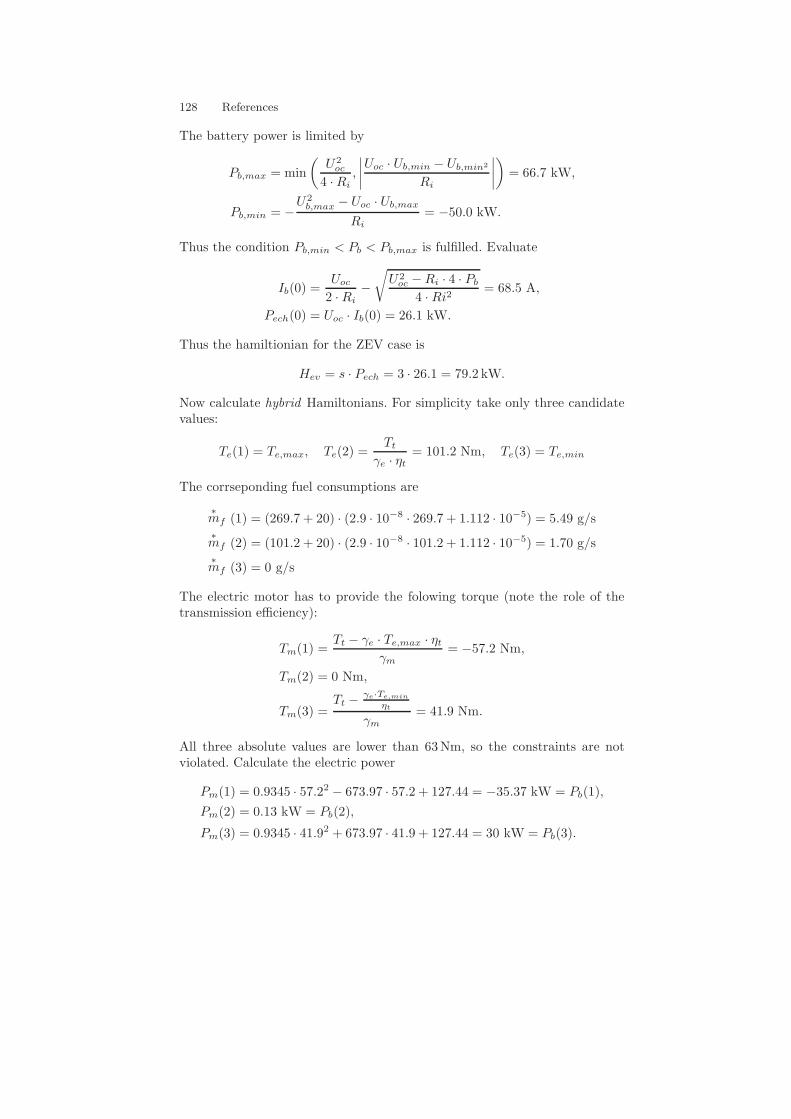
128 References
The battery power is limited by
Pb,max = min
(U2oc
4 ·Ri,
∣∣∣∣Uoc · Ub,min − Ub,min2
Ri
∣∣∣∣
)= 66.7 kW,
Pb,min = −U2b,max − Uoc · Ub,max
Ri= −50.0 kW.
Thus the condition Pb,min < Pb < Pb,max is fulfilled. Evaluate
Ib(0) =Uoc
2 · Ri−√
U2oc −Ri · 4 · Pb
4 · Ri2= 68.5 A,
Pech(0) = Uoc · Ib(0) = 26.1 kW.
Thus the hamiltionian for the ZEV case is
Hev = s · Pech = 3 · 26.1 = 79.2 kW.
Now calculate hybrid Hamiltonians. For simplicity take only three candidatevalues:
Te(1) = Te,max, Te(2) =Tt
γe · ηt= 101.2 Nm, Te(3) = Te,min
The corrseponding fuel consumptions are
∗mf (1) = (269.7 + 20) · (2.9 · 10−8 · 269.7 + 1.112 · 10−5) = 5.49 g/s∗mf (2) = (101.2 + 20) · (2.9 · 10−8 · 101.2 + 1.112 · 10−5) = 1.70 g/s∗mf (3) = 0 g/s
The electric motor has to provide the folowing torque (note the role of thetransmission efficiency):
Tm(1) =Tt − γe · Te,max · ηt
γm= −57.2 Nm,
Tm(2) = 0 Nm,
Tm(3) =Tt − γe·Te,min
ηt
γm= 41.9 Nm.
All three absolute values are lower than 63Nm, so the constraints are notviolated. Calculate the electric power
Pm(1) = 0.9345 · 57.22 − 673.97 · 57.2 + 127.44 = −35.37 kW = Pb(1),
Pm(2) = 0.13 kW = Pb(2),
Pm(3) = 0.9345 · 41.92 + 673.97 · 41.9 + 127.44 = 30 kW = Pb(3).
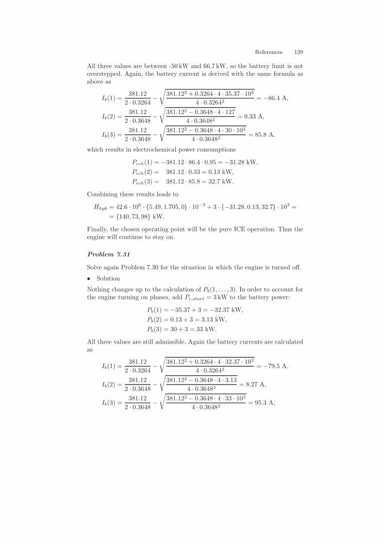
References 129
All three values are between -50 kW and 66.7 kW, so the battery limit is notoverstepped. Again, the battery current is derived with the same formula asabove as
Ib(1) =381.12
2 · 0.3264−√
381.122 + 0.3264 · 4 · 35.37 · 1034 · 0.32642
= −86.4 A,
Ib(2) =381.12
2 · 0.3648−√
381.122 − 0.3648 · 4 · 1274 · 0.36482
= 0.33 A,
Ib(3) =381.12
2 · 0.3648−√
381.122 − 0.3648 · 4 · 30 · 1034 · 0.36482
= 85.8 A,
which results in electrochemical power consumptions
Pech(1) = −381.12 · 86.4 · 0.95 = −31.28 kW,
Pech(2) = 381.12 · 0.33 = 0.13 kW,
Pech(3) = 381.12 · 85.8 = 32.7 kW.
Combining these results leads to
Hhyb = 42.6 · 106 · 5.49, 1.705, 0 · 10−3 + 3 · −31.28, 0.13, 32.7 · 103 =
= 140, 73, 98 kW.
Finally, the chosen operating point will be the pure ICE operation. Thus theengine will continue to stay on.
Problem 7.31
Solve again Problem 7.30 for the situation in which the engine is turned off.
• Solution
Nothing changes up to the calculation of Pb(1, . . . , 3). In order to account forthe engine turning on phases, add Pe,start = 3kW to the battery power:
Pb(1) = −35.37 + 3 = −32.37 kW,
Pb(2) = 0.13 + 3 = 3.13 kW,
Pb(3) = 30 + 3 = 33 kW.
All three values are still admissible. Again the battery currents are calculatedas
Ib(1) =381.12
2 · 0.3264−√
381.122 + 0.3264 · 4 · 32.37 · 1034 · 0.32642
= −79.5 A,
Ib(2) =381.12
2 · 0.3648−√
381.122 − 0.3648 · 4 · 3.134 · 0.36482
= 8.27 A,
Ib(3) =381.12
2 · 0.3648−√
381.122 − 0.3648 · 4 · 33 · 1034 · 0.36482
= 95.3 A,
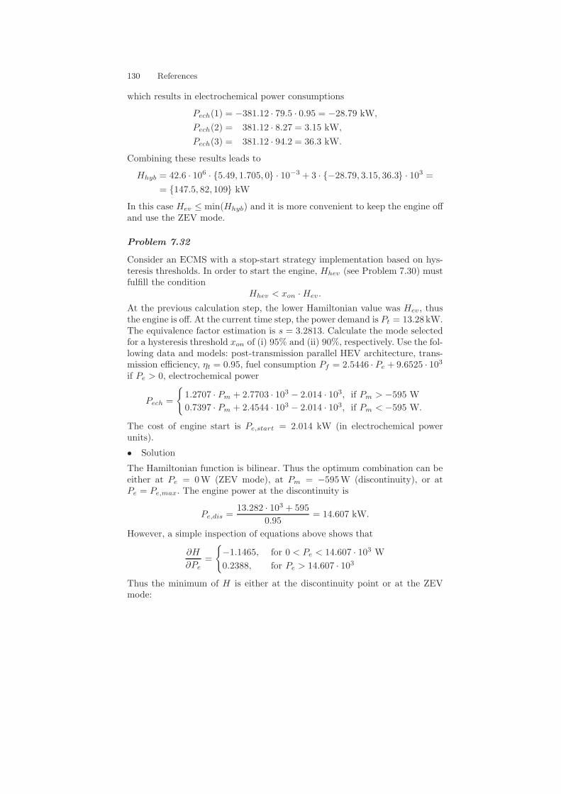
130 References
which results in electrochemical power consumptions
Pech(1) = −381.12 · 79.5 · 0.95 = −28.79 kW,
Pech(2) = 381.12 · 8.27 = 3.15 kW,
Pech(3) = 381.12 · 94.2 = 36.3 kW.
Combining these results leads to
Hhyb = 42.6 · 106 · 5.49, 1.705, 0 · 10−3 + 3 · −28.79, 3.15, 36.3 · 103 =
= 147.5, 82, 109 kW
In this case Hev ≤ min(Hhyb) and it is more convenient to keep the engine offand use the ZEV mode.
Problem 7.32
Consider an ECMS with a stop-start strategy implementation based on hys-teresis thresholds. In order to start the engine, Hhev (see Problem 7.30) mustfulfill the condition
Hhev < xon ·Hev.
At the previous calculation step, the lower Hamiltonian value was Hev, thusthe engine is off. At the current time step, the power demand is Pt = 13.28kW.The equivalence factor estimation is s = 3.2813. Calculate the mode selectedfor a hysteresis threshold xon of (i) 95% and (ii) 90%, respectively. Use the fol-lowing data and models: post-transmission parallel HEV architecture, trans-mission efficiency, ηt = 0.95, fuel consumption Pf = 2.5446 · Pe + 9.6525 · 103if Pe > 0, electrochemical power
Pech =
1.2707 · Pm + 2.7703 · 103 − 2.014 · 103, if Pm > −595 W
0.7397 · Pm + 2.4544 · 103 − 2.014 · 103, if Pm < −595 W.
The cost of engine start is Pe,start = 2.014 kW (in electrochemical powerunits).
• Solution
The Hamiltonian function is bilinear. Thus the optimum combination can beeither at Pe = 0W (ZEV mode), at Pm = −595W (discontinuity), or atPe = Pe,max. The engine power at the discontinuity is
Pe,dis =13.282 · 103 + 595
0.95= 14.607 kW.
However, a simple inspection of equations above shows that
∂H
∂Pe=
−1.1465, for 0 < Pe < 14.607 · 103 W
0.2388, for Pe > 14.607 · 103
Thus the minimum of H is either at the discontinuity point or at the ZEVmode:
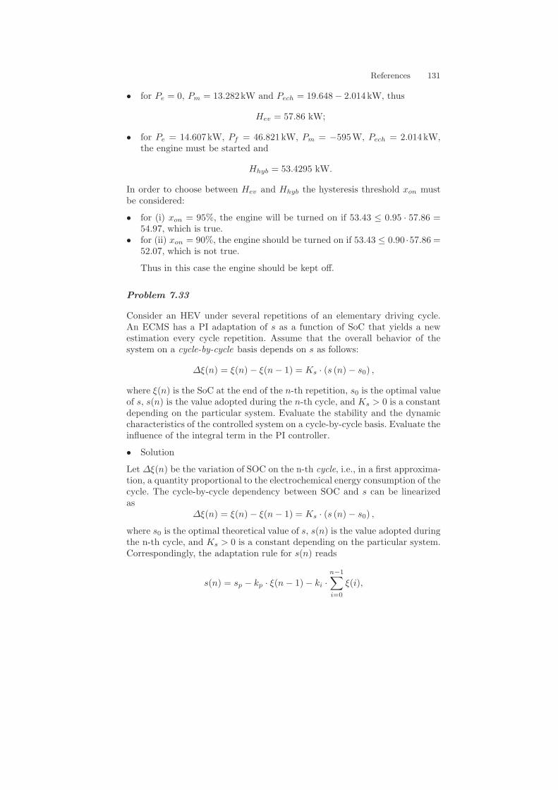
References 131
• for Pe = 0, Pm = 13.282kW and Pech = 19.648− 2.014kW, thus
Hev = 57.86 kW;
• for Pe = 14.607kW, Pf = 46.821kW, Pm = −595W, Pech = 2.014kW,the engine must be started and
Hhyb = 53.4295 kW.
In order to choose between Hev and Hhyb the hysteresis threshold xon mustbe considered:
• for (i) xon = 95%, the engine will be turned on if 53.43 ≤ 0.95 · 57.86 =54.97, which is true.
• for (ii) xon = 90%, the engine should be turned on if 53.43 ≤ 0.90 ·57.86 =52.07, which is not true.
Thus in this case the engine should be kept off.
Problem 7.33
Consider an HEV under several repetitions of an elementary driving cycle.An ECMS has a PI adaptation of s as a function of SoC that yields a newestimation every cycle repetition. Assume that the overall behavior of thesystem on a cycle-by-cycle basis depends on s as follows:
∆ξ(n) = ξ(n)− ξ(n− 1) = Ks · (s (n)− s0) ,
where ξ(n) is the SoC at the end of the n-th repetition, s0 is the optimal valueof s, s(n) is the value adopted during the n-th cycle, and Ks > 0 is a constantdepending on the particular system. Evaluate the stability and the dynamiccharacteristics of the controlled system on a cycle-by-cycle basis. Evaluate theinfluence of the integral term in the PI controller.
• Solution
Let ∆ξ(n) be the variation of SOC on the n-th cycle, i.e., in a first approxima-tion, a quantity proportional to the electrochemical energy consumption of thecycle. The cycle-by-cycle dependency between SOC and s can be linearizedas
∆ξ(n) = ξ(n)− ξ(n− 1) = Ks · (s (n)− s0) ,
where s0 is the optimal theoretical value of s, s(n) is the value adopted duringthe n-th cycle, and Ks > 0 is a constant depending on the particular system.Correspondingly, the adaptation rule for s(n) reads
s(n) = sp − kp · ξ(n− 1)− ki ·n−1∑
i=0
ξ(i),
132 References
where ∆ξ(0) = 0 by definition, kp > 0, ki ≥ 0 and sp initial value of s. Byshifting from the discrete time to the continuous time, and by combining thetwo equations, one obtains
d2s
dt2= −kp ·Ks ·
ds
dt− ki ·Ks · (s− s0).
This dynamics is stable. The factor s converges to s0 (unknown) as prescribed.Thus the quantity ∆x converges to 0. The true SOC error, the integral of ∆ξ,converges to zero as well (the prescribed value). The integral of the SOC errorconverges to the value (sp − s0)/ki.
If ki = 0, the SOC error does not vanish but it tends to (sp − s0)/kp.
Problem 7.34
Compare (7.22) with (7.27) – (7.31). Under which assumptions are they equiv-alent?
• Solution
Combining (7.27) – (7.31), obtain
s(t) = schg + (sdis − schg) · p(t) # schg + (sdis − schg) · (p0 + p1(t) ·Eech(t)) .
In the assumption that the difference Eh − Eh(t) # ∆Eh is kept constant(sliding horizon), the coefficient p1 is constant as well and
s(t) = schg + (sdis − schg) · p0 + (sdis − schg) · p1 · Ee(t).
The term Eech(t) is the electrochemical energy consumed. In terms of SOC,
Eech(t) = Q0 · (ξ(0)− ξ(t)) · Uoc(t)
and, assuming an averagely constant open-circuit voltage,
Eech(t) = K · (ξ(0)− ξ(t)) .
If ξ(0) = ξt, obtain (7.22) with
st = schg + (sdis − schg) · p0,kp = (sdis − schg) · p1 ·K.
Now give a closer look to p0 and p1. To simplify the analysis, assume ur =ul = 1 and neglect λ. Thus,
p0 =1ηe
1ηe
+ ηeand p1 =
1(1ηe
+ ηe)·∆Eh
.
References 133
Further impose (7.26)
1
ηe= sdis · ηf , ηe = schg · ηf
to find
p0 =sdis
sdis + schg
p1 =1
(sdis + schg) · ηf ·∆Em
st = schg + (sdis − schg) ·sdis
sdis + schg=
s2chg + s2dissdis + schg
.
It is easy to show that under the aforementioned assumptions schg < st < sdis,thus st plays the role of the constant optimal equivalence factor s0.
Problem 7.35
Express s0 as a function of ur, ul, sdis, and schg. Evaluate s0 for smax = 5,smin = 2, knowing from a cycle analysis that ur/ηe = 1.2 and ul · ηe = 1.8.
• Solution
Using the method of Problem 7.34, but with ur = ul, obtain
s0 =ul · s2c + ur · s2dur · sd + ul · sc
.
For the numerical case (smax = sd and smin = sc.
ηe =
√scsd
= 0.63
ur = 0.76
ul = 2.85
s0 =2.85 · 22 + 0.76 · 52
0.76 · 5 + 2.85 · 2= 3.2.
Remark: the value of ur found shows that pure ZEV would not be allowed inthis case.