Proceedings of the 2010 SIAM International Conference on Data Mining || Reconstruction from Randomized Graph via Low Rank Approximation

Reconstruction from Randomized Graph via Low Rank Approximation

Leting Wu, Xiaowei Ying, Xintao WuDepartment of Software and Information Systems

Univ. of North Carolina at Charlotte{lwu8,xying,xwu}@uncc.edu

AbstractThe privacy concerns associated with data analysis oversocial networks have spurred recent research on privacy-preserving social network analysis, particularly on privacy-preserving publishing of social network data. In this paper,we focus on whether we can reconstruct a graph from theedge randomized graph such that accurate feature valuescan be recovered. In particular, we present a low rankapproximation based reconstruction algorithm. We exploitspectral properties of the graph data and show why noisecould be separated from the perturbed graph using lowrank approximation. We also show key differences fromprevious findings of point-wise reconstruction methods onnumerical data through empirical evaluations and theoreticaljustifications.

1 IntroductionSocial networks are of significant importance in various ap-plication domains such as marketing, psychology, epidemi-ology and homeland security. The privacy concerns asso-ciated with data analysis over social networks have spurredrecent research on privacy-preserving social network anal-ysis, particularly on privacy-preserving publishing of socialnetwork data.

To protect privacy, one common practice is to publish anaive node-anonymized version of the network, e.g., by re-placing the identifying information of the nodes with randomIDs. While the naive node-anonymized network still permitsuseful analysis, as first pointed out in [4,14], this simple tech-nique does not guarantee privacy since adversaries may re-identify a target individual from the anonymized graph byexploiting some known structural information of his neigh-borhood.

The state-of-the-art anonymization methods on networkdata have three categories: K-anonymity privacy preser-vation via edge modification [17, 27, 28], edge randomiza-tion [14, 22–24], and clustering-based generalization [5, 7, 8,13, 26]. These above anonymization approaches have beenshown as a necessity in addition to naive anonymization topreserve privacy in publishing social network data.

In a social network, nodes usually correspond to indi-

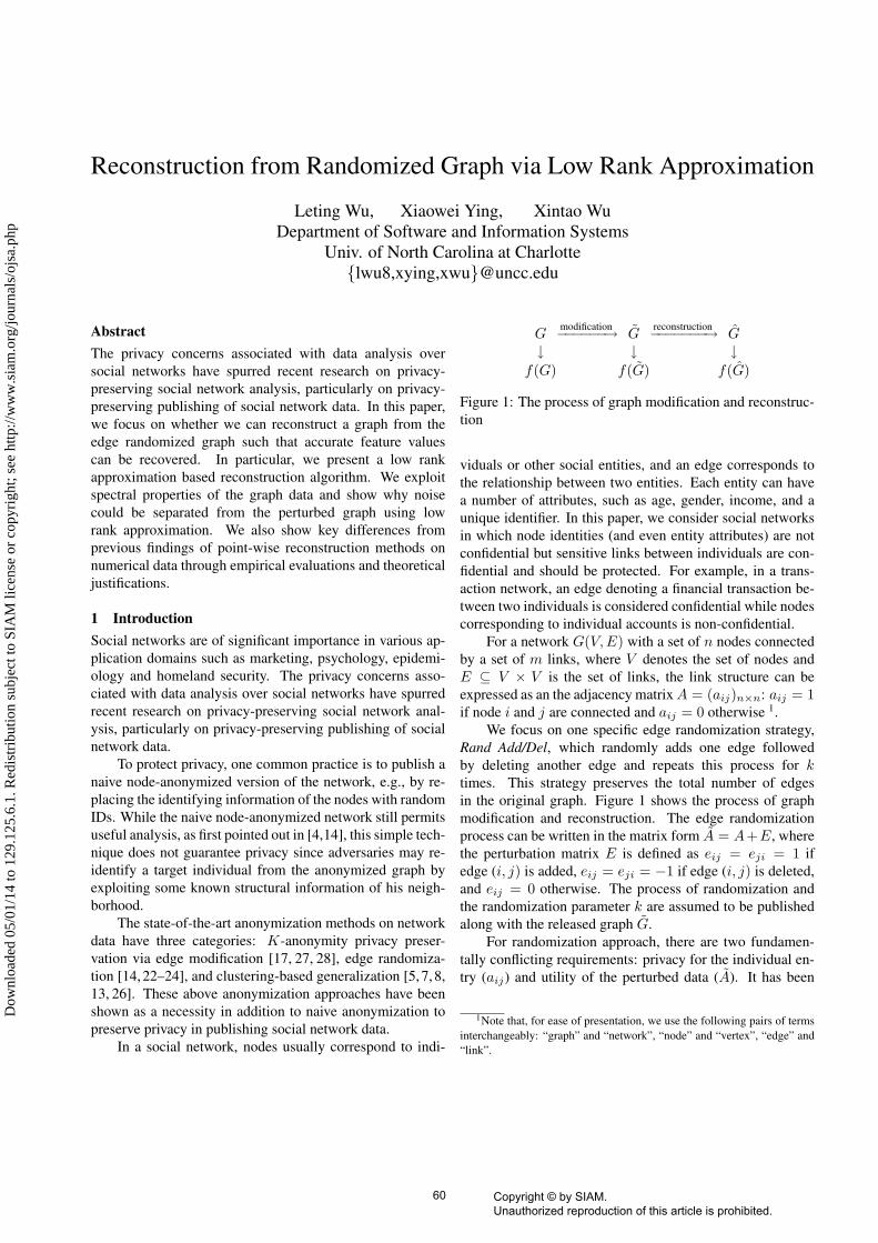
Gmodification−−−−−−→ G

reconstruction−−−−−−−→ G↓ ↓ ↓

f(G) f(G) f(G)

Figure 1: The process of graph modification and reconstruc-tion

viduals or other social entities, and an edge corresponds tothe relationship between two entities. Each entity can havea number of attributes, such as age, gender, income, and aunique identifier. In this paper, we consider social networksin which node identities (and even entity attributes) are notconfidential but sensitive links between individuals are con-fidential and should be protected. For example, in a trans-action network, an edge denoting a financial transaction be-tween two individuals is considered confidential while nodescorresponding to individual accounts is non-confidential.

For a network G(V, E) with a set of n nodes connectedby a set of m links, where V denotes the set of nodes andE ⊆ V × V is the set of links, the link structure can beexpressed as an the adjacency matrix A = (aij)n×n: aij = 1if node i and j are connected and aij = 0 otherwise 1.

We focus on one specific edge randomization strategy,Rand Add/Del, which randomly adds one edge followedby deleting another edge and repeats this process for ktimes. This strategy preserves the total number of edgesin the original graph. Figure 1 shows the process of graphmodification and reconstruction. The edge randomizationprocess can be written in the matrix form A = A+E, wherethe perturbation matrix E is defined as eij = eji = 1 ifedge (i, j) is added, eij = eji = −1 if edge (i, j) is deleted,and eij = 0 otherwise. The process of randomization andthe randomization parameter k are assumed to be publishedalong with the released graph G.

For randomization approach, there are two fundamen-tally conflicting requirements: privacy for the individual en-try (aij) and utility of the perturbed data (A). It has been

1Note that, for ease of presentation, we use the following pairs of termsinterchangeably: “graph” and “network”, “node” and “vertex”, “edge” and“link”.

60 Copyright © by SIAM. Unauthorized reproduction of this article is prohibited.

Dow

nloa

ded

05/0

1/14

to 1

29.1

25.6

.1. R

edis

trib

utio

n su

bjec

t to

SIA

M li

cens

e or

cop

yrig

ht; s

ee h

ttp://

ww

w.s

iam

.org

/jour

nals

/ojs

a.ph

p

shown in [14, 22] that a medium or large perturbation isneeded in order to protect the privacy of the individual entryunder feature based attacks or structural attacks. However,as shown in our empirical evaluation, the utility of the re-leased randomized graph (in terms of topological features) issignificantly lost in the randomized graph when a medium orlarge perturbation is applied.

To preserve utility, several advanced randomizationstrategies have been investigated recently. In [22], Ying andWu presented a randomization strategy that can preserve thespectral properties of the graph. They presented two spec-trum preserving randomization methods, Spctr Add/Del andSpctr Switch, which keep graph spectral characteristics (i.e.,the largest eigenvalue of the adjacency matrix and the sec-ond smallest eigenvalue of the Laplacian matrix) not muchchanged during randomization by examining eigenvectorvalues of nodes to choose where edges are added/deleted orswitched. In [12,23], the authors studied the problem of howto generate a synthetic graph matching given features of areal social network in addition to a given degree sequence.They proposed a Markov Chain based feature preserving ran-domization. Although the proposed advanced randomizationstrategies generally can preserve more structural properties,it is very challenging to quantify disclosure risks since theprocess of feature preserving strategies are complicated.

In this paper, we adopt a different approach. Wefocus on whether we can reconstruct a graph G from therandomized one G such that G is closer to the original graphG than G in terms of some feature f , i.e., |f(G)− f(G)| ≤|f(G) − f(G)|. In particular, we study the use of low rankapproximation approach to reconstruct structural featuresfrom the randomized graph. We exploit spectral propertiesof the graph data and show that the noise could be separatedfrom the perturbed graph.

1.1 Contribution Our contributions are as follows.

• We first propose the use of low rank approximation toreconstruct the graph topology from the randomizednetwork. While edge randomization can naturally beconsidered as an additive-noise perturbation, we shallshow those point-wise reconstruction methods [11, 15,16] developed in the numerical data setting are notapplicable in this network data setting. We also presenta novel solution to determine the (approximate) optimalrank, a key parameter in our reconstruction algorithm.

• To derive the low rank approximation based reconstruc-tion method for network data, we examine the relation-ship between graph topological structure and spectralspaces determined by eigen-pairs of the adjacency ma-trix. In particular, we discover that eigen-pairs of lead-ing positive eigenvalues capture the inner-communityconnection structure while eigen-pairs of leading neg-

ative eigenvalues capture the inter-community connec-tions.

• We explicitly assess effects of perturbation on the accu-racy of the reconstructed feature values. Our empiricalevaluation results show that accurate feature values canstill be recovered from the randomized graphs even withthe large magnitude of noise (e.g., k = 0.8m).

• One surprising finding is that, for most social networks,the reconstructed networks do not incur further disclo-sure risks of individual privacy than the released ran-domized graphs. This is very different from the nu-merical data setting. Our further investigation showsthat only networks with low ranks or a small number ofdominant eigenvalues may incur further privacy disclo-sure due to reconstruction.

1.2 Paper Organization The rest of this paper is orga-nized as follows. In Section 2, we first discuss topologicalfeatures used in this paper and revisit those low rank approx-imation based reconstruction methods on numerical data. InSection 3, we examine the spectra of network data and showthe relationship between the positive (negative) eigenvaluesand the reconstructed graph structure via low rank approxi-mation. In Section 4, we present our low rank approxima-tion based reconstruction algorithm. We also show our novelmethod to determine the optimal rank for low rank approxi-mation. We conduct empirical evaluations on three real so-cial networks in terms of both privacy and utility in Section5. In Section 6, we further examine what type of graphs aresensitive to low rank approximation based reconstruction interms of privacy protection. Finally we offer our concludingremarks and point out future directions in Section 7.

2 Preliminaries

Table 1: Notationsn, m number of nodes and edges

k number of edges added and deletedr number of eigen-pairs in low rank approximation

A(A) adjacency matrix of graph G (G)Ar (Ar) rank r approximation of A (A)

A adjacency matrix of the reconstructed graphλi, xi the ith largest eigenvalue in magnitude of A and

the corresponding eigenvectorE difference matrix, E = A−A

ε1 the largest eigenvalue of E in magnitude

2.1 Notation and Features We use the tilde conventionsto denote perturbations and use the hat conventions to denoteestimations. The original quantity is denoted by the samesymbol without a tilde or hat. Table 1 summarizes ournotations used in this paper.


Dow

nloa

ded

05/0

1/14

to 1

29.1

25.6

.1. R

edis

trib

utio

n su

bjec

t to

SIA

M li

cens

e or

cop

yrig

ht; s

ee h

ttp://

ww

w.s

iam

.org

/jour

nals

/ojs

a.ph

p

To understand and utilize the information in a network,researches have developed various measures to indicate thestructure and characteristics of the network from differentperspectives [10]. In this paper, we consider the followingtopological features of the graph:

• λ1, the largest eigenvalue of the adjacency matrix A.The eigenvalues of A encode information about thecycles of a network as well as its diameter. Themaximum degree, chromatic number, clique number,and extend of branching in a connected graph are allrelated to λ1. In [21], the authors studied how a viruspropagates in a real work and proved that the epidemicthreshold for a network is closely related to λ1.

• ν2, the second largest eigenvalue of the normal matrixN = D−1A. Let ν1 ≥ ν2 ≥ · · · ≥ νn denote theeigenvalues of N , ν1 ≡ 1. 1 − ν2 is the lower boundof the normal cut of the graph [19]. Therefore, ν2 isclose to 1 if the graph has a clear community structure,and the eigenvectors of ν2 is a good indicator of thecommunity partition.

• Q, modularity indicates the goodness of the communitystructure [10]. It is defined as the fraction of alledges that lie within communities minus the expectedvalue of the same quantity in a graph generated froma random model which keeps the expected number ofdegree for each node. A value Q = 0 indicates thatthe community structure is no stronger than would beexpected by random chance and high value other thanzero represents large deviations from randomness.

• C, transitivity measure is one type of clustering coef-ficient measure and characterizes the presence of lo-cal loops near a vertex. It is formally defined as C =3N∆/N3, where N∆ is the number of triangles and N3

is the number of connected triples.

Throughout this paper, we use the polblogs as an exam-ple. The polblogs network compiles the 16714 links among1222 US political blogs, based on incoming and outgoinglinks and posts during the time of the 2004 presidential elec-tion [1].

2.2 Low Rank Approximation based ReconstructionMethods on Numerical Data Revisited The low rank ap-proximation has been well investigated as a point-wise re-construction method in the numerical setting. In the settingof randomizing numerical data, a data set U with m recordsof n attributes is perturbed to U by an additive noise dataset V with same dimensions as U , i.e., U = U + V . Aspectral filtering based reconstruction method was first pro-posed in [16] to reconstruct original data values from the per-turbed data. Similar methods (e.g., PCA based reconstruc-tion method [15], SVD based reconstruction method [11])

have also been investigated. All methods exploited spectralproperties of the correlated data to remove the noise fromthe perturbed data set. This is because real-world numer-ical data is usually highly correlated in a low dimensionalspace while the randomly added noise is distributed (approx-imately) equally over all dimensions. Then, more accurateaggregate features can be reconstructed by projecting therandomized data into a proper low dimensional space wherethe majority information of the original data is preserved.

Spectral Filtering. The objective of the spectral filteringbased approach is to derive the estimation U of U from theperturbed data U based on random matrix theory. An explicitfiltering procedure is shown below.

1. Calculate the covariance matrix of U by Σ = UT U(assume U has mean equal to 0).

2. The covariance matrix Σ is symmetric and positivesemi-definite, we apply spectral decomposition on Σ toget its i-th largest eigenvalue λi and the correspondingeigenvector xi.

3. Derive the eigenvalues information from the covariancematrix of the noise V and choose a proper number ofdimensions, r.

4. Let Xr = [x1 x2 · · · xr], and the orthogonal projectionon to the subspace spanned by x1, . . . , xr is Pr =XrX

Tr . Obtain the estimated data set using U = UPr.

SVD. Singular value decomposition decomposes a matrixU ∈ Rm×n (say m ≥ n) as U =

∑ni=1 σipiq

Ti , where

σ1 ≥ σ2 ≥ · · · ≥ σn are the singular values and pi ∈ Rm

and qi ∈ Rn are the left and right singular vector of σi

respectively. Similarly, after perturbation U = U + V ,we have the SVD of U as U =

∑ni=1 σipiqi. The SVD

reconstruction method simply reconstructs U approximatelyas U = Ur =

∑ri=1 σipiq

Ti .

It has been shown that the spectral filtering method isequivalent to the SVD reconstruction method [11]. We canobserve that all spectral based methods reconstruct the orig-inal data by projecting the perturbed data onto the projectionsubspaces that are determined by the first r eigenvectors forthe spectral filtering method or by the first r singular vectorsfor the SVD method. The original spectral filtering algorithm[16] suggested using r = max{i|λi ≥ ε1} to determine thefirst r eigen components, where ε1 is the largest eigenvalueof the noise covariance matrix Cov(V ). The authors of [11]further proved that using r = max{i|λi ≥ 2ε1} can achieveapproximately optimal reconstruction for i.i.d. noise. This isbecause that it only includes the i-th eigen component whenthe benefit due to inclusion of the i-th component is greaterthan the loss due to the noise projected on the i-th compo-nent, i.e., λi ≥ 2ε1.


Dow

nloa

ded

05/0

1/14

to 1

29.1

25.6

.1. R

edis

trib

utio

n su

bjec

t to

SIA

M li

cens

e or

cop

yrig

ht; s

ee h

ttp://

ww

w.s

iam

.org

/jour

nals

/ojs

a.ph

p

3 Low Rank Approximation on Graph DataThe adjacency matrix A discussed here is different from thenumerical data set U and the covariance matrix Σ in thefollowing perspectives. First, A is a symmetric 0-1 matrixwhereas U is a numerical matrix and the covariance matrixΣ is a semi-definite one. Second, for numerical data, allthe eigenvalues of Σ are real and non-negative. For graphdata A, the covariance matrix is not properly defined. Wecan see that in AAT , the non-zero entry at row i column jmeans j is 2 steps away from i. When we directly applyeigen-decomposition on the adjacency matrix A, the eigen-decomposition of A contains negative eigenvalues.

In Section 3.1, we study the low rank approximation ongraph data. In Section 3.2, we examine the spectra of graphdata and show the relationship between the topological graphstructure and the significant eigen-pairs that may involveboth positive and negative eigenvalues.

3.1 Low Rank Approximation Let λi be A’s i-th largesteigenvalue in magnitude: |λ1| ≥ |λ2| ≥ · · · ≥ |λn|, and xi

denotes the eigenvector of λi. The rank r approximations ofA via the eigen-decomposition are given by:

(3.1) Ar =r∑

i=1

λixixTi .

Among all the matrix with rank no larger than r, the low rankapproximation Ar shown in (3.1) is the matrix closest to Ain term of the Frobenius norm [20]:

‖Ar −A‖2F = minrank(B)≤r

‖B −A‖2F .

The key difference between our low rank approximation ongraph data and those low rank approximation methods onnumerical data is that we rank eigenvalues based on theirabsolute values and also include those significant negativeeigenvalues in the low rank approximation. In Section 3.2,we will illustrate the relationship between the graph topologyand significant positive and negative eigenvalues.

Because Ar is a real matrix, we need to derive asymmetric 0-1 matrix A that is close to Ar. Our strategyis to find the 2m largest off-diagonal entries in Ar (note thatA and A are symmetric) and set the corresponding entries inA as 1 and others as 0, i.e.,

(3.2) A(i, j) =

{1, if Ar(i, j) is one of the 2m

largest off-diagonal entries,

0, otherwise.

By using (3.2), we have the following property.

PROPERTY 1. If A is obtained by (3.2), A is the closestadjacency matrix to Ar in term of the Frobenius norm, i.e.,

‖A−Ar‖2F = minB∈Am

n

‖B −Ar‖2F ,

whereAmn denotes the set of all symmetric n×n 0-1 matrices

with 2m off-diagonal 1’s and 0 else where.

The following theory states that the difference betweenthe spectrum of A and that of Ar is upper bounded by‖A−Ar‖2F .

THEOREM 1. [20] Given two n× n symmetric matrices Aand E with eigenvalues λ1 ≥ · · · ≥ λn and ε1 ≥ · · · ≥ εn

respectively. Let λ1 ≥ · · · ≥ λn be the eigenvalues ofA = A + E. Then we have

λi + εn ≤ λi ≤ λi + ε1,(3.3)∑

i(λi − λi)2 ≤ ‖E‖2F .(3.4)

By minimizing this upper bound, we expect the eigen-values and eigenvectors of A is close to those of A. In fact,many spectral properties, such as eigenvectors, the sum ofseveral eigenvalues, and spectral subspace, are stable whenthe magnitude of the difference matrix is moderate. Forvaries spectrum bounds and more details, please refer to [20].Since the graph topology is closely related with eigenvaluesand eigenvectors of the graph, we expect that A can preservethe major topological information of the original graph.

3.2 Leading Eigen-pairs vs. Graph Topology In thissection, we study the relationship between eigen-pairs andgraph topology. In particular, we examine the role of positiveand negative eigenvalues in graph topology.

Without loss of generality, we partition the node set Vinto two groups V1 = {1, . . . , n1} and V2 = {n1+1, . . . , n}.Then the adjacency matrix can be partitioned as

(3.5) A = Ainner+Ainter =(

A11 00 A22

)+

(0 A12

AT12 0

),

where A11 and A22 represent the edges within V1 and V2

respectively, and A12 represents the edges between V1 andV2.

Disconnected communities In an ideal graph with twodisconnected communities, A11 and A22 are dense matricesof comparable size, and A12 = 0. Then, all the eigenvaluesof A11 and A22 are eigenvalues of A. Let µ1 and η1 bethe largest eigenvalue in magnitude of A11 and A22 witheigenvector y1 and z1 respectively. µ1 and η1 are twoeigenvalues of A with eigenvectors

(y10

)and

(0z1

). Note

that, by the Perron-Frobenius theorem [9], µ1 and η1 mustbe positive and all entries in y1 and z1 must be positive.Assume µ1 ≥ η1, then

(3.6) A1 = µ1

(y1

0

)(yT

1 ,0) =(

µ1y1yT1 0

0 0

).


Dow

nloa

ded

05/0

1/14

to 1

29.1

25.6

.1. R

edis

trib

utio

n su

bjec

t to

SIA

M li

cens

e or

cop

yrig

ht; s

ee h

ttp://

ww

w.s

iam

.org

/jour

nals

/ojs

a.ph

p

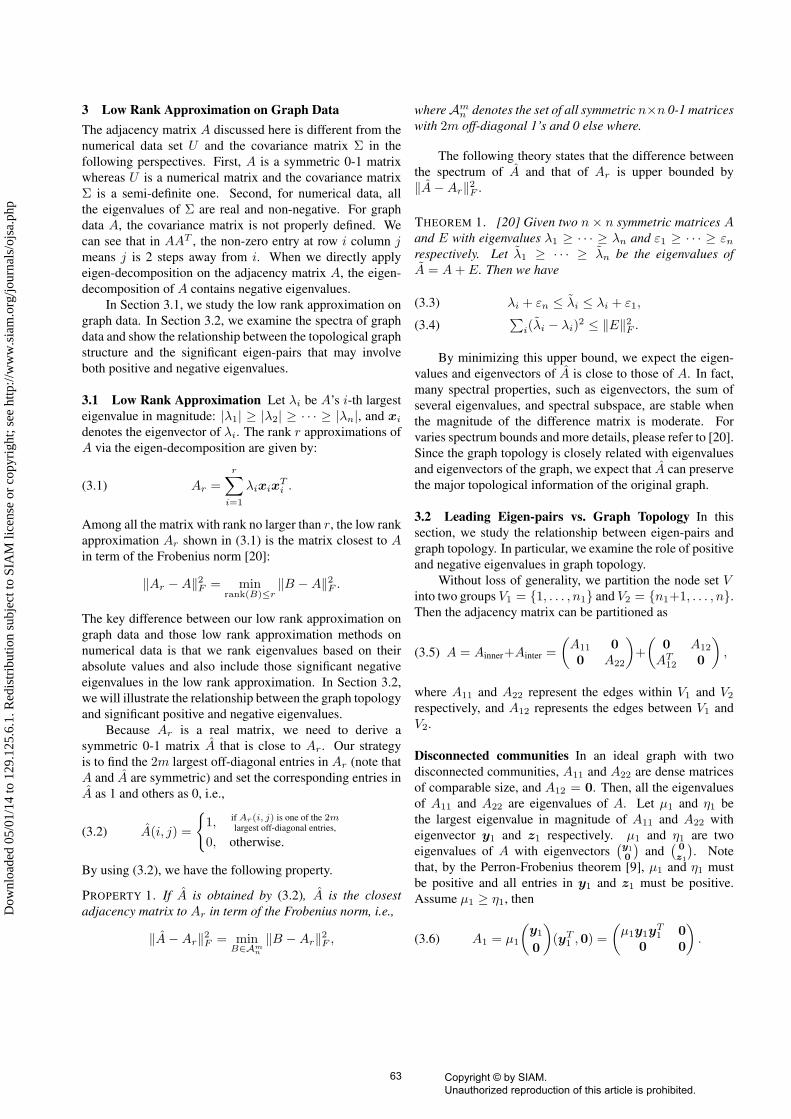
We can see all large entries only appear among the nodes inV1. Similarly, the rank 2 approximation of A is given by

(3.7) A2 =(

µ1y1yT1 0

0 η1z1zT1

),

and large entries appear both within V1 and V2. Figure 2shows a synthetic network with 60 nodes and 280 edges.This network contains two disconnected 30-node communi-ties generated via ER model with inner-community proba-bility 0.5. The derived graphs A by discretizing A1 and A2

via (3.2) are shown in Figure 2(b) and 2(c). For the graphderived from A1, all the edges appear in only one of thecommunities. After adding one more eigen-pair in the lowrank approximation, the derived graph shown in Figure 2(c)reveals two very clear communities.

(a) Original graph

(b) r = 1

(c) r = 2

Figure 2: Synthetic random graph with two disconnectedcommunities

Bipartite graph The negative eigenvalues are closely re-lated to the bipartite structure of the graph. A bipartite graphis a graph containing two types of nodes, and edges onlyexist between two nodes of different types. For a bipartitegraph, A11 and A22 in (3.5) are both zero matrix. The spec-trum of A is then fully determined by A12. Let σ ≥ 0 be thelargest singular value of A12 (note A12 is generally a non-square matrix) with right-singular value u and left-singularvalue v. If G is a connected graph, all the entries of u andv are positive. It is easy to verify that σ and −σ are both the

eigenvalues of A with eigenvalue(uv

)and

(−uv

)respectively.

Similar as (3.6) and (3.7), we can have

A1 =(

σuuT σuvT

σvuT σvvT

), A2 =

(0 2σuvT

2σvuT 0

).

We can see that entries within V1 and V2 in A1 are non-zero,which is significantly different from A. However, as weintroduce the leading negative eigenvalue, non-zero entriesin A2 only appear in those entries across two type of nodes.

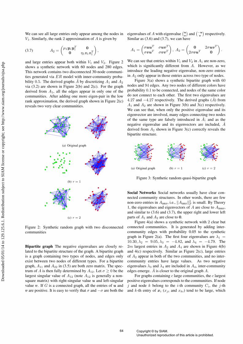
Figure 3(a) shows a synthetic bipartite graph with 60nodes and 94 edges. Any two nodes of different colors haveprobability 0.1 to be connected, and nodes of the same colordo not connect to each other. The first two eigenvalues are4.27 and −4.27 respectively. The derived graphs (A) fromA1 and A2 are shown in Figure 3(b) and 3(c) respectively.We can see that, when only the positive eigenvalue and itseigenvector are involved, many edges connecting two nodesof the same type are falsely introduced in A; and as thenegative eigenvalue and its eigenvectors are included, Aderived from A2 shown in Figure 3(c) correctly reveals thebipartite structure.

(a) Original graph (b) r = 1 (c) r = 2

Figure 3: Synthetic random quasi-bipartite graph

Social Networks Social networks usually have clear con-nected community structures. In other words, there are fewnon-zero entries in Ainter, i.e., ‖Ainter‖2F is small. By Theory1, the eigenvalues and eigenvectors of A are close to Ainner,and similar to (3.6) and (3.7), the upper right and lower leftparts of A1 and A2 are close to 0.

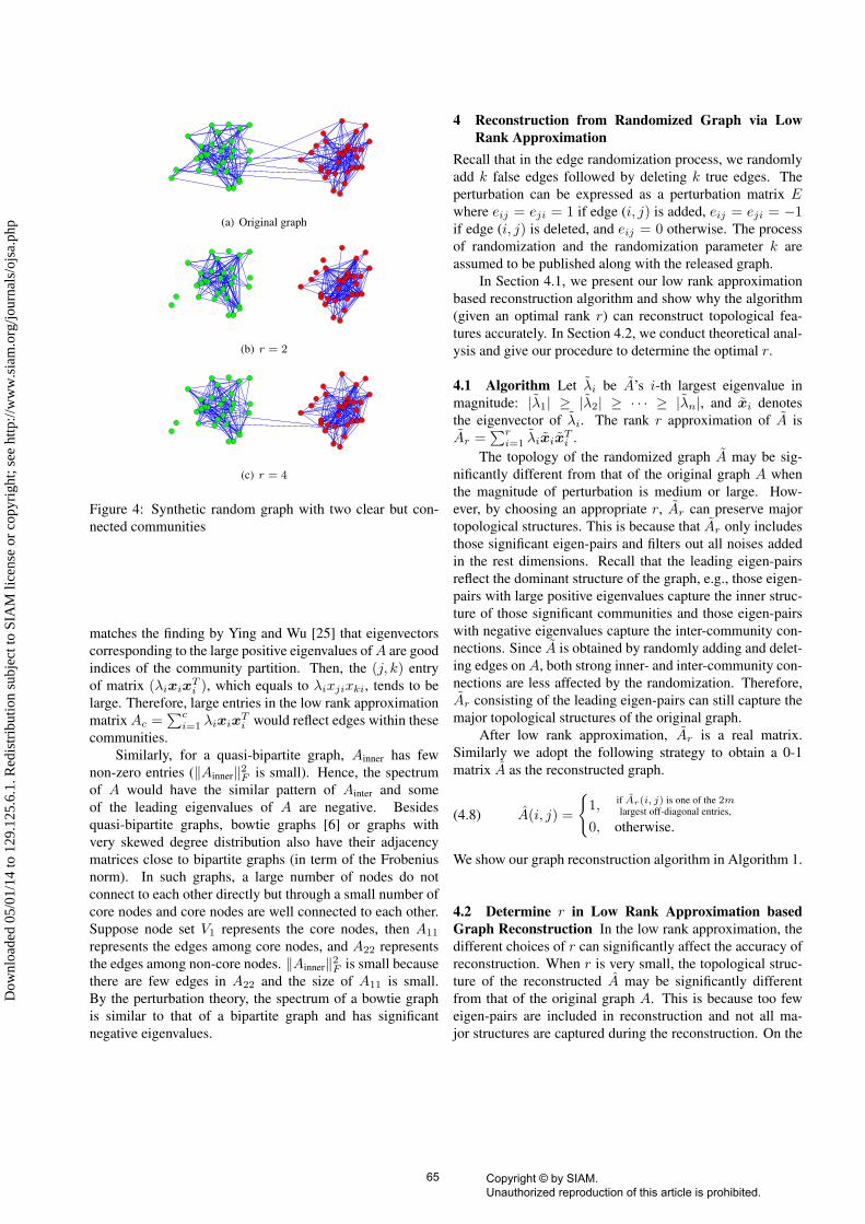
Figure 4(a) shows a synthetic network with 2 clear butconnected communities. It is generated by adding inter-community edges with probability 0.05 to the syntheticgraph in Figure 2(a). The first four eigenvalues are λ1 =10.30, λ2 = 9.05, λ3 = −4.82, and λ4 = −4.79. The2m largest entries in A2 and A4 are shown in Figure 4(b)and 4(c) respectively. Similar as Figure 2(c), large entriesof A2 appear in both of the two communities, and no inter-community entries have large values. As two negativeeigenvalues λ3 and λ4 are included in A4, inter-communityedges emerge. A is closer to the original graph A.

For graphs containing c large communities, the c largestpositive eigenvalues corresponds to the communities. If nodej and node k belong to the i-th community Ci, the j-thand k-th entry of xi (xji and xki) tend to be large, which


Dow

nloa

ded

05/0

1/14

to 1

29.1

25.6

.1. R

edis

trib

utio

n su

bjec

t to

SIA

M li

cens

e or

cop

yrig

ht; s

ee h

ttp://

ww

w.s

iam

.org

/jour

nals

/ojs

a.ph

p

(a) Original graph

(b) r = 2

(c) r = 4

Figure 4: Synthetic random graph with two clear but con-nected communities

matches the finding by Ying and Wu [25] that eigenvectorscorresponding to the large positive eigenvalues of A are goodindices of the community partition. Then, the (j, k) entryof matrix (λixix

Ti ), which equals to λixjixki, tends to be

large. Therefore, large entries in the low rank approximationmatrix Ac =

∑ci=1 λixix

Ti would reflect edges within these

communities.Similarly, for a quasi-bipartite graph, Ainner has few

non-zero entries (‖Ainner‖2F is small). Hence, the spectrumof A would have the similar pattern of Ainter and someof the leading eigenvalues of A are negative. Besidesquasi-bipartite graphs, bowtie graphs [6] or graphs withvery skewed degree distribution also have their adjacencymatrices close to bipartite graphs (in term of the Frobeniusnorm). In such graphs, a large number of nodes do notconnect to each other directly but through a small number ofcore nodes and core nodes are well connected to each other.Suppose node set V1 represents the core nodes, then A11

represents the edges among core nodes, and A22 representsthe edges among non-core nodes. ‖Ainner‖2F is small becausethere are few edges in A22 and the size of A11 is small.By the perturbation theory, the spectrum of a bowtie graphis similar to that of a bipartite graph and has significantnegative eigenvalues.

4 Reconstruction from Randomized Graph via LowRank Approximation

Recall that in the edge randomization process, we randomlyadd k false edges followed by deleting k true edges. Theperturbation can be expressed as a perturbation matrix Ewhere eij = eji = 1 if edge (i, j) is added, eij = eji = −1if edge (i, j) is deleted, and eij = 0 otherwise. The processof randomization and the randomization parameter k areassumed to be published along with the released graph.

In Section 4.1, we present our low rank approximationbased reconstruction algorithm and show why the algorithm(given an optimal rank r) can reconstruct topological fea-tures accurately. In Section 4.2, we conduct theoretical anal-ysis and give our procedure to determine the optimal r.

4.1 Algorithm Let λi be A’s i-th largest eigenvalue inmagnitude: |λ1| ≥ |λ2| ≥ · · · ≥ |λn|, and xi denotesthe eigenvector of λi. The rank r approximation of A isAr =

∑ri=1 λixix

Ti .

The topology of the randomized graph A may be sig-nificantly different from that of the original graph A whenthe magnitude of perturbation is medium or large. How-ever, by choosing an appropriate r, Ar can preserve majortopological structures. This is because that Ar only includesthose significant eigen-pairs and filters out all noises addedin the rest dimensions. Recall that the leading eigen-pairsreflect the dominant structure of the graph, e.g., those eigen-pairs with large positive eigenvalues capture the inner struc-ture of those significant communities and those eigen-pairswith negative eigenvalues capture the inter-community con-nections. Since A is obtained by randomly adding and delet-ing edges on A, both strong inner- and inter-community con-nections are less affected by the randomization. Therefore,Ar consisting of the leading eigen-pairs can still capture themajor topological structures of the original graph.

After low rank approximation, Ar is a real matrix.Similarly we adopt the following strategy to obtain a 0-1matrix A as the reconstructed graph.

(4.8) A(i, j) =

{1, if Ar(i, j) is one of the 2m

largest off-diagonal entries,

0, otherwise.

We show our graph reconstruction algorithm in Algorithm 1.

4.2 Determine r in Low Rank Approximation basedGraph Reconstruction In the low rank approximation, thedifferent choices of r can significantly affect the accuracy ofreconstruction. When r is very small, the topological struc-ture of the reconstructed A may be significantly differentfrom that of the original graph A. This is because too feweigen-pairs are included in reconstruction and not all ma-jor structures are captured during the reconstruction. On the


Dow

nloa

ded

05/0

1/14

to 1

29.1

25.6

.1. R

edis

trib

utio

n su

bjec

t to

SIA

M li

cens

e or

cop

yrig

ht; s

ee h

ttp://

ww

w.s

iam

.org

/jour

nals

/ojs

a.ph

p

Algorithm 1 Graph Reconstruction Algorithm

Input: randomized graph A, randomization parameter kOutput: reconstructed graph A

1: Calculate λi and xi, |λ1| ≥ · · · ≥ |λn|.2: Calculate λ∗1 using (4.9);3: r = 1;4: repeat5: Construct A from Ar =

∑ri=1 λixix

Ti by (4.8).

6: λ1 = the largest eigenvalue of A in magnitude;7: r = r + 1;8: until |λ1 − λ∗1| increases

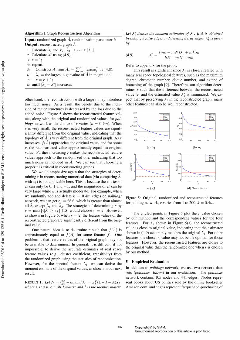
other hand, the reconstruction with a large r may introducetoo much noise. As a result, the benefit due to the inclu-sion of major structures is decreased by the loss due to theadded noise. Figure 5 shows the reconstructed feature val-ues, along with the original and randomized values, for pol-blogs network as the choice of r varies (k = 0.4m). Whenr is very small, the reconstructed feature values are signif-icantly different from the original value, indicating that thetopology of A is very different from the original graph. As rincreases, f(A) approaches the original value, and for somer, the reconstructed value approximately equals to originalvalue. Further increasing r makes the reconstructed featurevalues approach to the randomized one, indicating that toomuch noise is included in A. We can see that choosing aproper r is critical in reconstructing graphs.

We would emphasize again that the strategies of deter-mining r in reconstructing numerical data (via comparing λi

with ε1) is not applicable here. This is because the entries ofE can only be 0, 1 and −1, and the magnitude of E can bevery large while k is actually moderate. For example, whenwe randomly add and delete k = 0.4m edges on polblogsnetwork, we can get ε1 = 28.6, which is greater than almostall λi except λ1 and λ2. The strategies of determining r byr = max{i|λi ≥ ε1} [15] would choose r = 2. However,as shown in Figure 5, when r = 2, the feature values of thereconstructed graph are significantly different from the orig-inal value.

One natural idea is to determine r such that f(A) isapproximately equal to f(A) for some feature f . Oneproblem is that feature values of the original graph may notbe available to data miners. In general, it is difficult, if notimpossible, to derive the accurate estimates of real spacefeature values (e.g., cluster coefficient, transitivity) fromthe randomized graph using the statistics of randomization.However, for the spectral feature λ1, we can derive themoment estimate of the original values, as shown in our nextresult.

RESULT 1. Let N =(n2

)−m, and λ0 = xT1 (1− I− A)x1,

where 1 is a n × n all 1 matrix and I is the identity matrix.

Let λ∗1 denote the moment estimator of λ1. If A is obtainedby adding k false edges and deleting k true edges, λ∗1 is givenby

(4.9) λ∗1 =(mk −mN)λ1 + mkλ0

kN −mN + mk

Refer to appendix for the proof.This result is significant since λ1 is closely related with

many real space topological features, such as the maximumdegree, chromatic number, clique number, and extend ofbranching of the graph [9]. Therefore, our algorithm deter-mines r such that the difference between the reconstructedvalue λ1 and the estimated value λ∗1 is minimized. We ex-pect that by preserving λ1 in the reconstructed graph, manyother features can also be well reconstructed.

0 50 100 150 20040

60

80

100

120

140

160

r

λ 1

ReconOrigRand

(a) λ1

0 50 100 150 2000.5

0.6

0.7

0.8

0.9

1

r

ν 2

ReconOrigRand

(b) ν2

0 50 100 150 2000.5

1

1.5

2

r

Mod

ular

ity

ReconOrigRand

(c) Q

0 50 100 150 2000

0.2

0.4

0.6

0.8

r

Tra

sitiv

ity

ReconOrigRand

(d) Transitivity

Figure 5: Original, randomized and reconstructed featuresfor polblog network, r varies from 1 to 200, k = 0.4m.

The circled points in Figure 5 plot the r value chosenby our method and the corresponding values for the fourfeatures. For λ1 shown in Figure 5(a), the reconstructedvalue is close to original value, indicating that the estimatorshown in (4.9) accurately matches the original λ1. For otherfeatures, the chosen r value may not be the optimal for thosefeatures. However, the reconstructed features are closer tothe original value than the randomized one when r is chosenby our method.

5 Empirical EvaluationIn addition to polblogs network, we use two network datasets (polbooks, Enron) in our evaluation. The polbooksnetwork contains 105 nodes and 441 edges. Nodes repre-sent books about US politics sold by the online booksellerAmazon.com, and edges represent frequent co-purchasing of


Dow

nloa

ded

05/0

1/14

to 1

29.1

25.6

.1. R

edis

trib

utio

n su

bjec

t to

SIA

M li

cens

e or

cop

yrig

ht; s

ee h

ttp://

ww

w.s

iam

.org

/jour

nals

/ojs

a.ph

p

books by the same buyers.2 The Enron network was builtfrom an email corpus of a real organization over the coursecovering a 3 years period. We used a pre-processed ver-sion of the dataset provided by [18]. This data set contains252,759 emails from 151 Enron employees, mainly seniormanagers. We regard there is an edge between node i andj if there are at least 5 emails sent between i and j, whichresults in 869 edges. The numbers of nodes and edges forthree networks are shown in the first row of Table 2.

5.1 Feature Reconstruction We focus on four topologi-cal features (λ1, ν2, Q, and C) in our evaluation. For eachnetwork data set, we first calculate feature values of the orig-inal graph and show them in Table 2. We randomize eachnetwork data with noise level k

m = 0.4. We then apply ourlow rank approximation based reconstruction algorithm oneach randomized graph and calculate the reconstructed fea-ture values from the reconstructed graph. The randomizationand reconstruction process repeats 10 times. We report theaverage results of these 10 rounds in Table 2.

We can observe that perturbation with noise level km =

0.4 significantly changes the feature values in the random-ized graphs. It indicates that edge randomization in generalcannot well preserve the graph topological structure. How-ever, for all four features on three network data sets, ourreconstructed feature values are much closer to the originalones.

To evaluate accuracy of feature reconstruction, we usethe following measure.

DEFINITION 5.1. For a graph feature f , define reconstruc-tion quality

Sf = 1− |f(A)− f(A)||f(A)− f(A)| .

Sf ∈ (0, 1] indicates that the reconstructed feature iscloser to the original feature value than the feature valuedirectly calculated from the randomized graph. The largerSf is, the better the feature is reconstructed. Sf = 1 if andonly if f(A) = f(A), and Sf is close to 1 if f(A) ≈ f(A).

Table 2 shows the reconstruction quality Sf for thesefour features on three networks (k = 0.4m). We can seethat all Sf values are above 0.22 and some Sf values areeven close to 1, indicating that the majority of topologicalstructure of the original graph has been reconstructed. Wealso notice that λ1 is better reconstructed than the other threefeatures. This is because we use the estimate of λ1 as ourtarget function when we determine r.

Effect of Noise Level In this experiment, we evaluatehow the reconstruction accuracy of features is affected

2polbooks and polblogs are available at http://www-personal.umich.edu/˜mejn/netdata/.

by the magnitude of noise. We set noise level km =

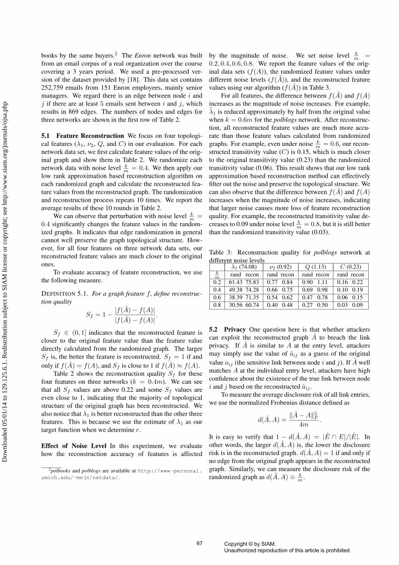
0.2, 0.4, 0.6, 0.8. We report the feature values of the orig-inal data sets (f(A)), the randomized feature values underdifferent noise levels (f(A)), and the reconstructed featurevalues using our algorithm (f(A)) in Table 3.

For all features, the difference between f(A) and f(A)increases as the magnitude of noise increases. For example,λ1 is reduced approximately by half from the original valuewhen k = 0.6m for the polblogs network. After reconstruc-tion, all reconstructed feature values are much more accu-rate than those feature values calculated from randomizedgraphs. For example, even under noise k

m = 0.6, our recon-structed transitivity value (C) is 0.15, which is much closerto the original transitivity value (0.23) than the randomizedtransitivity value (0.06). This result shows that our low rankapproximation based reconstruction method can effectivelyfilter out the noise and preserve the topological structure. Wecan also observe that the difference between f(A) and f(A)increases when the magnitude of noise increases, indicatingthat larger noise causes more loss of feature reconstructionquality. For example, the reconstructed transitivity value de-creases to 0.09 under noise level k

m = 0.8, but it is still betterthan the randomized transitivity value (0.03).

Table 3: Reconstruction quality for polblogs network atdifferent noise levels

λ1 (74.08) ν2 (0.92) Q (1.13) C (0.23)km

rand recon rand recon rand recon rand recon0.2 61.43 75.83 0.77 0.84 0.90 1.11 0.16 0.220.4 49.38 74.28 0.66 0.75 0.69 0.98 0.10 0.190.6 38.39 71.35 0.54 0.62 0.47 0.78 0.06 0.150.8 30.56 60.74 0.40 0.48 0.27 0.50 0.03 0.09

5.2 Privacy One question here is that whether attackerscan exploit the reconstructed graph A to breach the linkprivacy. If A is similar to A at the entry level, attackersmay simply use the value of aij as a guess of the originalvalue aij (the sensitive link between node i and j). If A wellmatches A at the individual entry level, attackers have highconfidence about the existence of the true link between nodei and j based on the reconstructed aij .

To measure the average disclosure risk of all link entries,we use the normalized Frobenius distance defined as

d(A, A) =‖A−A‖2F

4m.

It is easy to verify that 1 − d(A, A) = |E ∩ E|/|E|. Inother words, the larger d(A, A) is, the lower the disclosurerisk is in the reconstructed graph. d(A, A) = 1 if and only ifno edge from the original graph appears in the reconstructedgraph. Similarly, we can measure the disclosure risk of therandomized graph as d(A, A) ≡ k

m .


Dow

nloa

ded

05/0

1/14

to 1

29.1

25.6

.1. R

edis

trib

utio

n su

bjec

t to

SIA

M li

cens

e or

cop

yrig

ht; s

ee h

ttp://

ww

w.s

iam

.org

/jour

nals

/ojs

a.ph

p

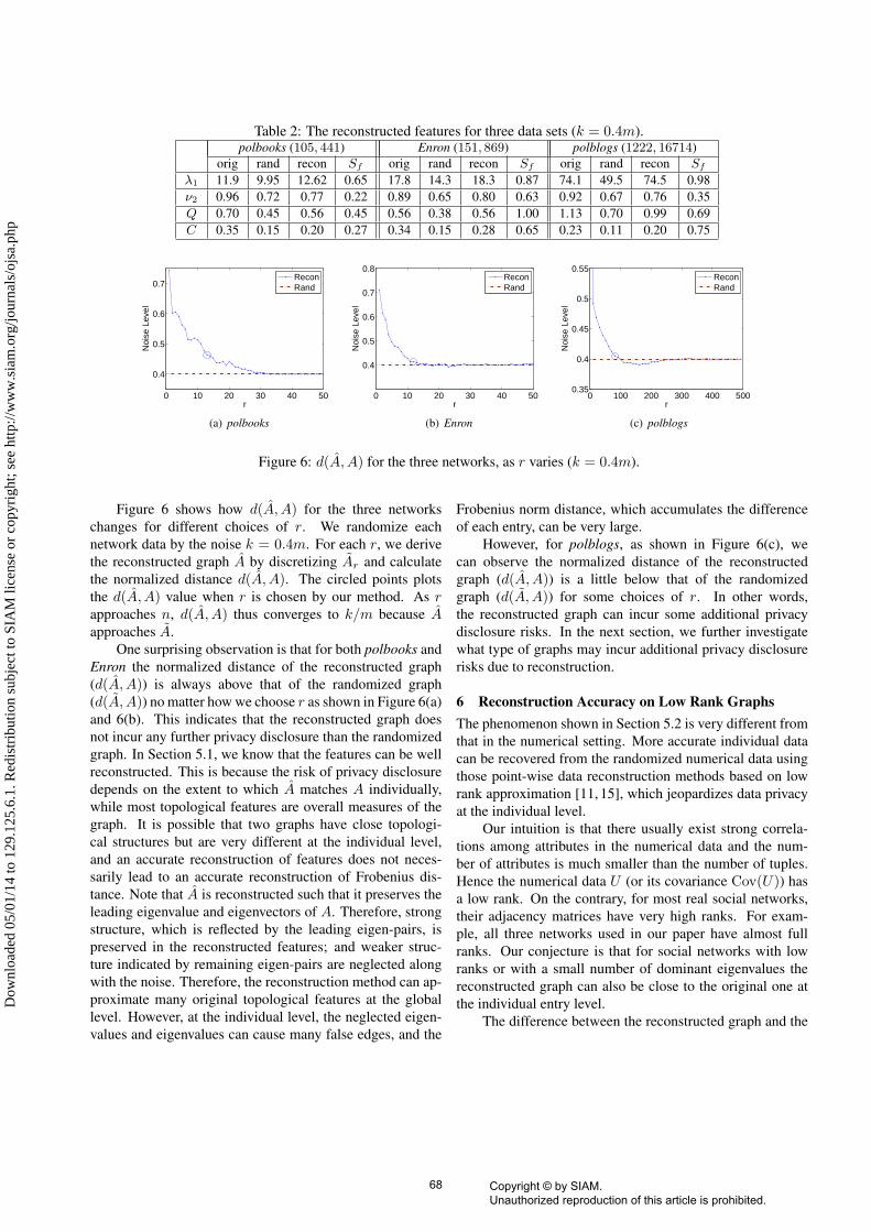
Table 2: The reconstructed features for three data sets (k = 0.4m).polbooks (105, 441) Enron (151, 869) polblogs (1222, 16714)

orig rand recon Sf orig rand recon Sf orig rand recon Sf

λ1 11.9 9.95 12.62 0.65 17.8 14.3 18.3 0.87 74.1 49.5 74.5 0.98ν2 0.96 0.72 0.77 0.22 0.89 0.65 0.80 0.63 0.92 0.67 0.76 0.35Q 0.70 0.45 0.56 0.45 0.56 0.38 0.56 1.00 1.13 0.70 0.99 0.69C 0.35 0.15 0.20 0.27 0.34 0.15 0.28 0.65 0.23 0.11 0.20 0.75

0 10 20 30 40 50

0.4

0.5

0.6

0.7

r

Noi

se L

evel

ReconRand

(a) polbooks

0 10 20 30 40 50

0.4

0.5

0.6

0.7

0.8

r

Noi

se L

evel

ReconRand

(b) Enron

0 100 200 300 400 5000.35

0.4

0.45

0.5

0.55

r

Noi

se L

evel

ReconRand

(c) polblogs

Figure 6: d(A, A) for the three networks, as r varies (k = 0.4m).

Figure 6 shows how d(A, A) for the three networkschanges for different choices of r. We randomize eachnetwork data by the noise k = 0.4m. For each r, we derivethe reconstructed graph A by discretizing Ar and calculatethe normalized distance d(A, A). The circled points plotsthe d(A, A) value when r is chosen by our method. As rapproaches n, d(A, A) thus converges to k/m because Aapproaches A.

One surprising observation is that for both polbooks andEnron the normalized distance of the reconstructed graph(d(A, A)) is always above that of the randomized graph(d(A, A)) no matter how we choose r as shown in Figure 6(a)and 6(b). This indicates that the reconstructed graph doesnot incur any further privacy disclosure than the randomizedgraph. In Section 5.1, we know that the features can be wellreconstructed. This is because the risk of privacy disclosuredepends on the extent to which A matches A individually,while most topological features are overall measures of thegraph. It is possible that two graphs have close topologi-cal structures but are very different at the individual level,and an accurate reconstruction of features does not neces-sarily lead to an accurate reconstruction of Frobenius dis-tance. Note that A is reconstructed such that it preserves theleading eigenvalue and eigenvectors of A. Therefore, strongstructure, which is reflected by the leading eigen-pairs, ispreserved in the reconstructed features; and weaker struc-ture indicated by remaining eigen-pairs are neglected alongwith the noise. Therefore, the reconstruction method can ap-proximate many original topological features at the globallevel. However, at the individual level, the neglected eigen-values and eigenvalues can cause many false edges, and the

Frobenius norm distance, which accumulates the differenceof each entry, can be very large.

However, for polblogs, as shown in Figure 6(c), wecan observe the normalized distance of the reconstructedgraph (d(A, A)) is a little below that of the randomizedgraph (d(A, A)) for some choices of r. In other words,the reconstructed graph can incur some additional privacydisclosure risks. In the next section, we further investigatewhat type of graphs may incur additional privacy disclosurerisks due to reconstruction.

6 Reconstruction Accuracy on Low Rank GraphsThe phenomenon shown in Section 5.2 is very different fromthat in the numerical setting. More accurate individual datacan be recovered from the randomized numerical data usingthose point-wise data reconstruction methods based on lowrank approximation [11, 15], which jeopardizes data privacyat the individual level.

Our intuition is that there usually exist strong correla-tions among attributes in the numerical data and the num-ber of attributes is much smaller than the number of tuples.Hence the numerical data U (or its covariance Cov(U)) hasa low rank. On the contrary, for most real social networks,their adjacency matrices have very high ranks. For exam-ple, all three networks used in our paper have almost fullranks. Our conjecture is that for social networks with lowranks or with a small number of dominant eigenvalues thereconstructed graph can also be close to the original one atthe individual entry level.

The difference between the reconstructed graph and the


Dow

nloa

ded

05/0

1/14

to 1

29.1

25.6

.1. R

edis

trib

utio

n su

bjec

t to

SIA

M li

cens

e or

cop

yrig

ht; s

ee h

ttp://

ww

w.s

iam

.org

/jour

nals

/ojs

a.ph

p

original graph can be divided into three components:

‖A− A‖F = ‖(A−Ar) + (Ar − Ar) + (Ar − A)‖F

≤ ‖A−Ar‖F + ‖Ar − Ar‖F + ‖Ar − A‖F .(6.10)

‖A − Ar‖F denotes the low rank approximation errorthat is determined by those excluded non-significant eigen-pairs; ‖Ar − Ar‖F denotes the randomization error thatis determined by the noise added in the subspace spannedby the first r eigenvectors; and ‖Ar − A‖F denotes thediscretization error when we convert the real matrix Ar to the0-1 matrix A. To decrease ‖A− Ar‖F , we tend to choose alarge r value. However, a large r value introduces more noisein the projected spectral space, increasing the randomizationerror ‖Ar − Ar‖F .

Hence, if a graph A can be well approximated by Ar

with a small r value, both the low rank approximation error(‖A − Ar‖F ) and the randomization error (‖Ar − Ar‖F )could be small. In this case, Ar ≈ Ar ≈ A, and Ar isalready close to a 0-1 matrix, which then further reduces thediscretization error ‖A− A‖F .

For three network data sets used in our paper, we can de-rive their minimum r values such that ‖A−Ar‖2F

‖A‖2F≤ τ . When

τ = 0.05, we have r = 54 (0.51n) for polbooks, r = 64(0.42n) for Enron, and r = 348 (0.28n) for polblogs net-work. Since all r values are large, the difference between thereconstructed graph and the original graph at the individuallevel (‖A−A‖F ) is still significant, indicating the individualprivacy is well protected in the reconstructed graph. How-ever, the feature values can still be well reconstructed. Thisis because those non-significant eigen-pairs do not contributemuch to the global topological structure although they maysignificantly affect the Frobenius distance.

To verify our proposition, we construct a series ofsynthetic graphs Ht (t = 2, 5, 10, 50, 100, 200) from thepolblog network. We first calculate At =

∑ti=1 λixix

Ti

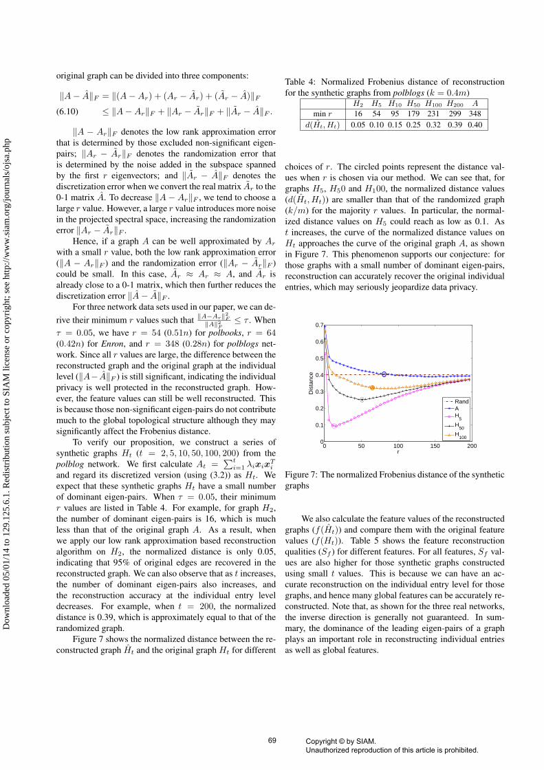
and regard its discretized version (using (3.2)) as Ht. Weexpect that these synthetic graphs Ht have a small numberof dominant eigen-pairs. When τ = 0.05, their minimumr values are listed in Table 4. For example, for graph H2,the number of dominant eigen-pairs is 16, which is muchless than that of the original graph A. As a result, whenwe apply our low rank approximation based reconstructionalgorithm on H2, the normalized distance is only 0.05,indicating that 95% of original edges are recovered in thereconstructed graph. We can also observe that as t increases,the number of dominant eigen-pairs also increases, andthe reconstruction accuracy at the individual entry leveldecreases. For example, when t = 200, the normalizeddistance is 0.39, which is approximately equal to that of therandomized graph.

Figure 7 shows the normalized distance between the re-constructed graph Ht and the original graph Ht for different

Table 4: Normalized Frobenius distance of reconstructionfor the synthetic graphs from polblogs (k = 0.4m)

H2 H5 H10 H50 H100 H200 A

min r 16 54 95 179 231 299 348d(Ht, Ht) 0.05 0.10 0.15 0.25 0.32 0.39 0.40

choices of r. The circled points represent the distance val-ues when r is chosen via our method. We can see that, forgraphs H5, H50 and H100, the normalized distance values(d(Ht,Ht)) are smaller than that of the randomized graph(k/m) for the majority r values. In particular, the normal-ized distance values on H5 could reach as low as 0.1. Ast increases, the curve of the normalized distance values onHt approaches the curve of the original graph A, as shownin Figure 7. This phenomenon supports our conjecture: forthose graphs with a small number of dominant eigen-pairs,reconstruction can accurately recover the original individualentries, which may seriously jeopardize data privacy.

0 50 100 150 2000

0.1

0.2

0.3

0.4

0.5

0.6

0.7

r

Dis

tanc

e

RandAH

5

H50

H100

Figure 7: The normalized Frobenius distance of the syntheticgraphs

We also calculate the feature values of the reconstructedgraphs (f(Ht)) and compare them with the original featurevalues (f(Ht)). Table 5 shows the feature reconstructionqualities (Sf ) for different features. For all features, Sf val-ues are also higher for those synthetic graphs constructedusing small t values. This is because we can have an ac-curate reconstruction on the individual entry level for thosegraphs, and hence many global features can be accurately re-constructed. Note that, as shown for the three real networks,the inverse direction is generally not guaranteed. In sum-mary, the dominance of the leading eigen-pairs of a graphplays an important role in reconstructing individual entriesas well as global features.


Dow

nloa

ded

05/0

1/14

to 1

29.1

25.6

.1. R

edis

trib

utio

n su

bjec

t to

SIA

M li

cens

e or

cop

yrig

ht; s

ee h

ttp://

ww

w.s

iam

.org

/jour

nals

/ojs

a.ph

p

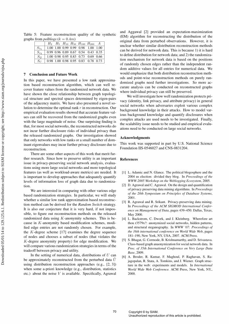
Table 5: Feature reconstruction quality of the syntheticgraphs from polblogs (k = 0.4m)

H2 H5 H10 H50 H100 H200 A

Sλ1 1.00 1.00 0.99 0.99 0.98 1.00 1.00Sν2 0.99 0.96 0.89 0.67 0.54 0.43 0.35SQ 1.00 0.98 0.95 0.83 0.73 0.69 0.66SC 0.98 1.00 0.98 0.95 0.83 0.78 0.73

7 Conclusion and Future WorkIn this paper, we have presented a low rank approxima-tion based reconstruction algorithm, which can well re-cover feature values from the randomized network data. Wehave shown the close relationship between graph topologi-cal structure and spectral spaces determined by eigen-pairsof the adjacency matrix. We have also presented a novel so-lution to determine the optimal rank r in reconstruction. Ourempirical evaluation results showed that accurate feature val-ues can still be recovered from the randomized graphs evenwith the large magnitude of noise. One surprising finding isthat, for most social networks, the reconstructed networks donot incur further disclosure risks of individual privacy thanthe released randomized graphs. Our investigation showedthat only networks with low ranks or a small number of dom-inant eigenvalues may incur further privacy disclosure due toreconstruction.

There are some other aspects of this work that merit fur-ther research. Since how to preserve utility is an importantissue in privacy-preserving social network analysis, evalua-tions using more large social networks and more topologicalfeatures (as well as workload-aware metrics) are needed. Itis important to develop approaches that adequately quantifylevels of information loss of graph data due to randomiza-tion.

We are interested in comparing with other various edgebased randomization strategies. In particular, we will studywhether a similar low rank approximation based reconstruc-tion method can be derived for the Random Switch strategy.It is also our conjecture that it is very hard, if not impos-sible, to figure out reconstruction methods on the releasedrandomized data using K-anonymity schemes. This is be-cause in K-anonymity based modification schemes, modi-fied edge entries are not randomly chosen. For example,the K-degree scheme [17] examines the degree sequenceof nodes and chooses a subset of nodes (that violates theK-degree anonymity property) for edge modification. Wewill compare various randomization strategies in terms of thetradeoff between privacy and utility.

In the setting of numerical data, distributions of U canbe approximately reconstructed from the perturbed data Uusing distribution reconstruction approaches (e.g., [2, 3])when some a-priori knowledge (e.g., distribution, statisticsetc.) about the noise V is available. Specifically, Agrawal

and Aggawal [2] provided an expectation-maximization(EM) algorithm for reconstructing the distribution of theoriginal data from perturbed observations. However, it isunclear whether similar distribution reconstruction methodscan be derived for network data. This is because 1) it is hardto define distribution for network data; and 2) the randomiza-tion mechanism for network data is based on the positionsof randomly chosen edges rather than the independent ran-dom additive values for all entries for numerical data. Wewould emphasize that both distribution reconstruction meth-ods and point-wise reconstruction methods on purely ran-domized graphs need further investigations. So more ac-curate analysis can be conducted on reconstructed graphswhere individual privacy can still be preserved.

We will investigate how well randomization protects pri-vacy (identity, link privacy, and attribute privacy) in generalsocial networks when adversaries exploit various complexbackground knowledge in their attacks. How to model var-ious background knowledge and quantify disclosures whencomplex attacks are used needs to be investigated. Finally,the scalability issue needs to be studied and empirical evalu-ations need to be conducted on large social networks.

AcknowledgmentsThis work was supported in part by U.S. National ScienceFoundation IIS-0546027 and CNS-0831204.

References

[1] L. Adamic and N. Glance. The political blogosphere and the2004 us election: divided they blog. In Proceedings of theWWW-2005 Workshop on the Weblogging Ecosystem, 2005.

[2] D. Agrawal and C. Agrawal. On the design and quantificationof privacy preserving data mining algorithms. In Proceedingsof the 20th Symposium on Principles of Database Systems,2001.

[3] R. Agrawal and R. Srikant. Privacy-preserving data mining.In Proceedings of the ACM SIGMOD International Confer-ence on Management of Data, pages 439–450. Dallas, Texas,May 2000.

[4] L. Backstrom, C. Dwork, and J. Kleinberg. Wherefore artthou r3579x?: anonymized social networks, hidden patterns,and structural steganography. In WWW ’07: Proceedings ofthe 16th international conference on World Wide Web, pages181–190, New York, NY, USA, 2007. ACM Press.

[5] S. Bhagat, G. Cormode, B. Krishnamurthy, and D. Srivastava.Class-based graph anaonymization for social network data. InProc. of 35th International Conference on Very Large DataBase, 2009.

[6] A. Broder, R. Kumar, F. Maghoul, P. Raghavan, S. Ra-jagopalan, R. Stata, A. Tomkins, and J. Wiener. Graph struc-ture in the web: experiments and models. In InternationalWorld Wide Web Conference. ACM Press, New York, NY.,2000.


Dow

nloa

ded

05/0

1/14

to 1

29.1

25.6

.1. R

edis

trib

utio

n su

bjec

t to

SIA

M li

cens

e or

cop

yrig

ht; s

ee h

ttp://

ww

w.s

iam

.org

/jour

nals

/ojs

a.ph

p

[7] A. Campan and T. M. Truta. A clustering approach for dataand structural anonymity in social networks. In PinKDD,2008.

[8] G. Cormode, D. Srivastava, T. Yu, and Q. Zhang. Anonymiz-ing bipartite graph data using safe groupings. In Proc. ofVLDB08, pages 833–844, 2008.

[9] D. Cvetkovic, P. Rowlinson, and S. Simic. Eigenspaces ofGraphs. Cambridge University Press, 1997.

[10] L. da F. Costa, F. A. Rodrigues, G. Travieso, and P. R. V.Boas. Characterization of complex networks: A survey ofmeasurements. Advances In Physics, 56:167, 2007.

[11] S. Guo, X. Wu, and Y. Li. Determining error bounds forspectral filtering based reconstruction methods in privacypreserving data mining. Knowl. Inf. Syst., 17(2):217–240,2008.

[12] S. Hanhijarvi, G. C. Garriga, and K. Puolamaki. Randomiza-tion techniques for graphs. In Proc. of the 9th SIAM Confer-ence on Data Mining, 2009.

[13] M. Hay, G. Miklau, D. Jensen, D. Towsely, and P. Weis.Resisting structural re-identification in anonymized socialnetworks. In VLDB, 2008.

[14] M. Hay, G. Miklau, D. Jensen, P. Weis, and S. Srivastava.Anonymizing social networks. University of MassachusettsTechnical Report, 07-19, 2007.

[15] Z. Huang, W. Du, and B. Chen. Deriving private informationfrom randomized data. In Proceedings of the ACM SIGMODConference on Management of Data. Baltimore, MA, 2005.

[16] H. Kargupta, S. Datta, Q. Wang, and K. Sivakumar. Onthe privacy preserving properties of random data perturbationtechniques. In Proc. of the 3rd Int’l Conf. on Data Mining,pages 99–106, 2003.

[17] K. Liu and E. Terzi. Towards identity anonymization ongraphs. In Proceedings of the ACM SIGMOD Conference,Vancouver, Canada, 2008. ACM Press.

[18] J. Shetty and J. Adibi. The Enron email dataset databaseschema and brief statistical report. Information SciencesInstitute Technical Report, University of Southern California,2004.

[19] J. Shi and J. Malik. Normalized cuts and image segmenta-tion. In CVPR ’97: Proceedings of the 1997 Conference onComputer Vision and Pattern Recognition (CVPR ’97), page731, Washington, DC, USA, 1997. IEEE Computer Society.

[20] G. W. Stewart and J. guang Sun. Matrix Perturbation Theory.Academic Press, 1990.

[21] Y. Wang, D. Chakrabarti, C. Wang, and C. Faloutsos. Epi-demic spreading in real networks: An eigenvalue viewpoint.Proceedings of the 22nd International Symposium on ReliableDistributed Systems, 2003.

[22] X. Ying and X. Wu. Randomizing social networks: aspectrum preserving approach. In Proc. of the 8th SIAMConference on Data Mining, April 2008.

[23] X. Ying and X. Wu. Graph generation with prescribed featureconstraints. In Proc. of the 9th SIAM Conference on DataMining, 2009.

[24] X. Ying and X. Wu. On link privacy in randomizing socialnetworks. In PAKDD, 2009.

[25] X. Ying and X. Wu. On randomness measures for socialnetworks. In SDM, 2009.

[26] E. Zheleva and L. Getoor. Preserving the privacy of sensitiverelationships in graph data. In PinKDD, pages 153–171,2007.

[27] B. Zhou and J. Pei. Preserving privacy in social networksagainst neighborhood attacks. In Proceedings of the 24thInternational Conference on Data Engineering (ICDE’08),2008.

[28] L. Zou, L. Chen, and M. T. Ozsu. k-automorphism: A generalframework for privacy preserving network publication. InProc. of 35th International Conference on Very Large DataBase, 2009.

A Proof of Result 1Define λ0 = xT

1 (1− I−A)x1 and λ0 = xT1 (1− I− A)x1.

Since λ1 = xT1 Ax1, we have

(1.11) E(λ1) = E(xT1 Ax1) ≈ xT

1 E(A)x1.

We adopt the assumption that x1 ≈ x1 in establishing thesecond equality of (1.11). Since in Rand Add/Del everyexisting (non-existing) edge of A has the same probabilityto be add (deleted), we have E(aij) = m−k

m if aij = 1, andE(aij) = k

N if aij = 0 and i 6= j, where N =(n2

)−m, i.e.,

E(A) =m− k

mA +

k

N(1− I −A).

Continue with (1.11), we have

E(λ1) =m− k

mxT

1 Ax1 +k

NxT

1 (1− I −A)x1

= (1− k

m)λ1 +

k

Nλ0.

Similarly, we can calculate E(λ0) and have

E(λ1) = (1− km )λ1 + k

N λ0,

E(λ0) = (1− kN )λ1 + k

mλ0.(1.12)

In estimating λ1, we substitute E(λ1) and E(λ0) withobserved λ1 and λ0, and solving (1.12) for λ0 and λ1, wecan get the moment estimator of λ1 is given by:

λ∗1 =(mk −mN)λ1 + mkλ0

kN −mN + mk.


Dow

nloa

ded

05/0

1/14

to 1

29.1

25.6

.1. R

edis

trib

utio

n su

bjec

t to

SIA

M li

cens

e or

cop

yrig

ht; s

ee h

ttp://

ww

w.s

iam

.org

/jour

nals

/ojs

a.ph

p

Documents

Proceedings of the 2010 SIAM International Conference on Data Mining || Reconstruction from Randomized Graph via Low Rank Approximation