Embed Size (px)
Citation preview
UNIVERSITAT DE BARCELONAFacultat de Biologia
Departament d'Ecologia
Tesi doctoral
PROCESOS HETEROTRÒFICS MICROBIANSA L’EMBASSAMENT DE SAU
HETEROTROPHIC MICROBIAL PROCESSESIN THE SAU RESERVOIR
Marta Comerma
Barcelona, febrer del 2003

“..no riñais a la niña por estar siempre absorta… de mayor será científica!”Alfredo Comerma
A mis abuelos,a mis padres,
a mis hermanosy a Juan Carlos,
gracias por estar ahí.

3
INDEX
Index 3
Agraïments 5
Introducció 9
Introduction 21The microbial food web: components and their importance in the pelagic food web 23Spatial heterogeneity in reservoirs, longitudinal zonation 28Study site and state of the art 31Objectives of this study 36
Material and Methods 39Samplings 41Physical and chemical parameters 42Biological parameters 47
Chapter 1: "LONGITUDINAL CIRCULATION PATTERNS IN THE
SAU RESERVOIR” 57Abstract 59Introduction 60Results and discussion 61
The annual pattern of longitudinal water circulation 61Seasonal patterns of stratification and river circulation 64The horizontal organization of the Sau Reservoir and the Plunge Point 68
Concluding remarks 73
Chapter 2: “EFFECTS OF WATER CIRCULATION ON NUTRIENT DYNAMICS" 75Abstract 77Introduction 78Results and discussion 79
The reservoir as a “water purifying plant” 79Horizontal chemical gradients controlled by river circulation patterns 86
Concluding remarks 88
Chapter 3: "PLANKTONIC FOOD WEB STRUCTURE ALONG THE SAU
RESERVOIR (SPAIN) IN SUMMER 1997" 89Abstract 91Introduction 92Sampling and methodological remarks 94Results 94
4
Development of physical and chemical parameters and chlorophyll a 94Longitudinal trophic succession 96Bacterial production and protistan bacterivory 97Zooplankton 99
Discussion 101
Chapter 4: "SEASONAL CHANGES IN THE EPILIMNETIC MICROBIAL
FOOD WEB DYNAMICS ALONG A EUTROPHIC RESERVOIR" 107Abstract 109Introduction 110Methodological remarks 111Results 113
Seasonal and spatial changes in protistan abundance, bacterial production and grazing 113Spatial food web succession versus hydrology 116Main genera of ciliates in the Sau Reservoir and their role 118
Discussion 122
Chapter 5: "CARBON FLOW DYNAMICS IN THE PELAGIC COMMUNITY
OF THE SAU RESERVOIR" 127Abstract 129Introduction 130Sampling and methodological remarks 131Results 132Discussion 138
Chapter 6: "BOTTOM-UP AND TOP-DOWN FACTORS CONTROLLING
PROTOZOAN GROWTH IN A EUTROPHIC RESERVOIR" 145Abstract 147Introduction 148Methodological remarks 149Results 151
Protozoan growth rates 152Ciliate community composition and doubling times 156Zooplankton 157
Discussion 158
References 161
Resum 177
Conclusions 189
AGRAÏMENTS

Agraïments
7
AGRAÏMENTS
Talment com una cursa d’orientació… tot un repte! Una gran aventura que ja arribat a unfinal, que no la fi.
Un bon dia el Joan Armengol em va oferir un mapa per on fer una bonica i llarga cursad’orientació, jo vaig acceptar i, de seguida, em van aconsellar la millor brúixola del mercat, enKarel Šimek. Un, quasi m’ha fet de pare, i, l’altre, m’ha donat molt més que una bona basecientífica, un punt de referència en tot moment i una molt bona amistat.
La inscripció a la cursa m’ha estat possible gràcies a una Beca de Formació d’Investigadorsdel Programa Propi de la Universitat de Barcelona, a qui també haig d’agrair els ajuts perestades curtes a l’estranger, que durant quatre anys seguits m’han permès visitar l’Institutd’Hidrobiologia Txec.
En començar, davant del mapa tot et sembla igual. Però no, mirant i mirant, trobes aquellselements de referència que et fan situar i t’ajuden a prendre decisions. Aquí és on haigd’agrair a la gent del GREAC la seva bona acollida, el seu suport, la seva companyia. Al Sergili vull agrair la mirada crítica al meu primer article, en vaig aprendre molt. Al Quico, lesinteressants converses per tornar cap a Mataró… La Isabel sempre m’ha animat molt.L’Helena, l’Anna Mª, l’Andrea, la Cesca, l’Eulàlia, el Joan, l’Enrique, la Núria, les Montses,Anna… buf! no sabeu tot el què he après amb vosaltres (a fer anar programes, a fer gràfics, atrobar les coses i treballar al laboratori, …), m’heu donat molta seguretat en el camí. Però emquedo amb lo més important, la vostra amistat. Als que heu vingut després, Esther, Susana,Rafa, Eli, David, Vicenç, Mari, Gora, Ainoha, … també us haig d’agrair molts bons moments.Sou un gran equip.
Comencem a córrer, buscant la primera fita… i allà veig un corredor que s’atura buscantcom jo. Juan Carlos, el meu company per a la resta de la cursa, i de totes les curses quevinguin. Gràcies per la teva paciència, saps que m’ha fet servei moltes vegades.
Ai els “embalseros”! Uns altres corredors sense descans. Feina dura! Oi Joan! però gràciesa tu, sempre rient. Amb el Rafa encara al·lucino del que es pot arribar a treballar. I la Mari, ésla formigueta que no està mai quieta. I si no, pregunteu a tots aquells que han estat a Sau. ElsTxecs (Jirka, Pepa i Honza), Maria, Dolors, Susana, Constantin, Claudia… a tots els ha tocattreballar de valent. Susanna, quina portada de tesi més maca gràcies a tú! Ara tenen el relleuel Luciano, l’Enrique, el Jaime, voltant pels altres “embass”. I no menys feina fa el David ambel Foix. Gràcies a tots.
Agraïments
8
Bé, la cursa va bé, ja portes un parell de fites i en el camí d’una a l’altre et vas trobant méscorredors, que van en direccions molt diverses, tots tenen la seva traça,… i sempre tenscuriositat per saber cap a on van. Jose, Xavi de P., Marc V., Teresa, Fede, Sergi, Pere, Olga,Marta, Marisol, Núria, Xavi Ll., Mireia, Miquel Àngel, Chechu, Marc P., Salvador, Carolina,Oliver, Bernat H., Bernat L., Toni, Fiona, Montserrat, … alguns heu estat companys de cursesde veritat, altres, companys d’excursions o fins i tot de viatges, i tots m’heu donat molt bonesconverses amb cafè inclòs.
Més fites per endavant, això és un no parar. Com els incansables companys d’Aigües TerLlobregat, mes a mes, sempre interessats en l’evolució de Sau i en allò què hi anem esbrinantels ecòlegs. Gràcies pel suport tècnic, però sobretot pel suport humà: Antonio, Jose Javier,Fernado G., Fernando V., Fran i Albert.
Ara és el moment perillós de la cursa, perquè amb el cansament és fàcil despistar-se.Persones com l’Antonio Vidal, el Pep Gasol, la Dolors Planes, l’Humbert Salvador, el MirekMacek, el Jirka Nedona, el Pepa Hezlar, el Jaroslav Vrba, el Milan Straskrava, la VeraStraskravova i tots els professors del Departament d’Ecologia amb el seu immens vagatgehan ajudat a que jo sempre pogués aprendre quelcom més de l’Ecologia Microbiana.
Quan les forces comencen a defallir… avituallament. Sense la família Morilla i la bona gentde Sau les campanyes no hagueren estat el mateix. El Pavel sempre ha tingut un bon àpatTxec que servir-me per esmorzar. El Carmelo amb les seves coques i la Carmen amb elsseus cuinats també m’han donat forces pel camí.
Cal no perdre temps i buscar el millor i més ràpid camí d’una fita a l’altre. Aquí haig d’agrairel Suport Tècnic i personal dels Serveis Científico-tècnics, i en especial a tot l’equip d’AnàlisiGeoquímic (Anna Mª, Jaume, Laia i Eva). I també a tot l’equip de l’Institut d’Hidrobiologia Txeca Ceske Budejovice, que tan amablement m’han acollit a les seves instal·lacions.
Ja estic al tram final de cursa, no m’ho crec, espero no haver-me deixat cap fita! A totsaquells que no us he donat les gràcies més explícitament espero que em doneu l’oportunitatde fer-ho en persona, el paper té fi però no el munt de records que m’emporto d’aquestacursa.
I a l’arribada, et retrobes amb aquells que no has vist, però sempre han estat allà per donar-te una acollida ben càlida. Gràcies al suport incondicional de la meva família. Gràcies a totsels membres de la Secció de Ciències Naturals del Museu de Mataró i a tots els companysdel Museu per oferir-me un bon ambient de feina. Gràcies al Club Oros de Mataró per la salutcontagiosa. A l’Anna, l’Aina, la Mari i la Ruth, gràcies pels ànims quan més ho he necessitat.

INTRODUCCIÓ

Introducció
11
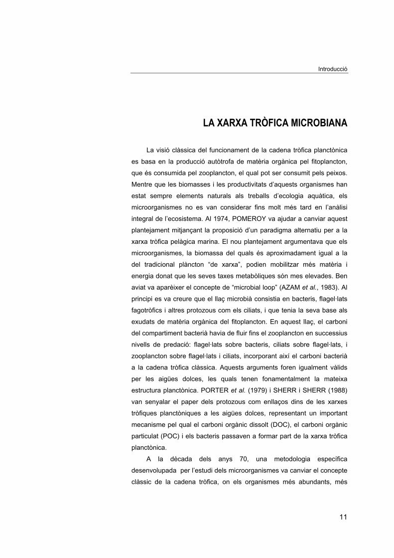
LA XARXA TRÒFICA MICROBIANA
La visió clàssica del funcionament de la cadena tròfica planctònica
es basa en la producció autòtrofa de matèria orgànica pel fitoplancton,
que és consumida pel zooplancton, el qual pot ser consumit pels peixos.
Mentre que les biomasses i les productivitats d’aquests organismes han
estat sempre elements naturals als treballs d’ecologia aquàtica, els
microorganismes no es van considerar fins molt més tard en l’anàlisi
integral de l’ecosistema. Al 1974, POMEROY va ajudar a canviar aquest
plantejament mitjançant la proposició d’un paradigma alternatiu per a la
xarxa tròfica pelàgica marina. El nou plantejament argumentava que els
microorganismes, la biomassa del quals és aproximadament igual a la
del tradicional plàncton “de xarxa”, podien mobilitzar més matèria i
energia donat que les seves taxes metabòliques són mes elevades. Ben
aviat va aparèixer el concepte de “microbial loop” (AZAM et al., 1983). Al
principi es va creure que el llaç microbià consistia en bacteris, flagel·lats
fagotròfics i altres protozous com els ciliats, i que tenia la seva base als
exudats de matèria orgànica del fitoplancton. En aquest llaç, el carboni
del compartiment bacterià havia de fluir fins el zooplancton en successius
nivells de predació: flagel·lats sobre bacteris, ciliats sobre flagel·lats, i
zooplancton sobre flagel·lats i ciliats, incorporant així el carboni bacterià
a la cadena tròfica clàssica. Aquests arguments foren igualment vàlids
per les aigües dolces, les quals tenen fonamentalment la mateixa
estructura planctònica. PORTER et al. (1979) i SHERR i SHERR (1988)
van senyalar el paper dels protozous com enllaços dins de les xarxes
tròfiques planctòniques a les aigües dolces, representant un important
mecanisme pel qual el carboni orgànic dissolt (DOC), el carboni orgànic
particulat (POC) i els bacteris passaven a formar part de la xarxa tròfica
planctònica.
A la dècada dels anys 70, una metodologia específica
desenvolupada per l’estudi dels microorganismes va canviar el concepte
clàssic de la cadena tròfica, on els organismes més abundants, més
Introducció
12
permanents, més diversificats i més àmpliament distribuïts havien estat
ignorats (PEDRÓS-ALIÓ, C. i GUERRERO, R., 1994). La microscopia
d’epifluorescència (PORTER and FEIG, 1980) i les tècniques amb
isòtops radioactius (RIEMANN, 1984; KIRCHMANN et al., 1985) van fer
possible el descobriment de nous organismes més actius i abundants del
que es pensava fins llavors. Des dels anys 80 fins a mitjans dels anys 90,
un interès creixent es va abocar a la incidència, la taxonomia i la
funcionalitat dels organismes microbians del plàncton. Malgrat que
l’esforç es va fer a tota mena d’ambients aquàtics, els resultats més
coherents van sorgir de l’estudi dels ecosistemes marins.
Les noves informacions sobre el paper que juguen els bacteris i el
protozous planctònics revelen que les interaccions dels microorganismes
són més complexes que el que es recollia en les descripcions inicials.
Bona part de la producció primària és canalitzada a través de diversos
compartiments del llaç microbià en forma de DOC i POC, abans de ser
disponible per al zooplancton. En cossos d’aigua temperats i tropicals,
els microorganismes poden arribar a consumir més de la meitat de
l’energia fixada per la fotosíntesi (POMEROY i WIEBE, 1988). El DOC
autòcton que és utilitzat pels bacteris no procedeix únicament dels
fotosintats exudats per les algues (RIEMANN i S0NDERGARD, 1986),
sinó que fan servir també DOC excretat pel zooplancton, derivat de
l’activitat d’alimentació del zooplancton (LAMPERT, 1978), i el que prové
de la lisi de bacteris i fitoplancton produïda per l’activitat dels virus
(BRATBAK et al., 1992). Al llarg de la darrera dècada, les quantitats de
virus reportats en diversos sistemes marins i d’aigua dolça han estat molt
elevades (108 virus ml-1; BERGH et al., 1989; HARA et al., 1991;
MARANGER i BIRD, 1995), i sembla ser que constitueixen un
component molt dinàmic de la comunitat microbiana. Mitjançant la
infecció d’organismes cel·lulars i la subsegüent lisi, l’activitat dels virus
alimenta la respiració i la producció heteròtrofa bacteriana. La predació
dels protozous a les aigües dolces pot controlar les abundàncies
bacterianes (BERNINGER et al., 1991). Els flagel·lats i els ciliats petits
també poden regular la biomassa i l’espectre de mides del
picofitoplancton (WEHR, 1991). Els ciliats més grans (>100 µm)
s’alimenten en canvi de bacterioplancton i nanofitoplancton. Rotífers
Introducció
13
(ARNDT, 1993) i copèpods (WICKMAN, 1995; DOBBERFUHL et al.,
1997) són consumidors eficients del fitoplancton i de tots el components
del llaç microbià (bacteris, nanoflagel·lats heteròtrofs i ciliats). Algunes
espècies de cladòcers (especialment Daphnia) s’alimenten de partícules
de la mida de les bactèries i competeixen amb els protozous pel carboni i
la resta de nutrients (SANDERS i PORTER, 1990; PACE et al., 1990;
PACE i FUNKE, 1991). Resumint, els bacteris i els seus consumidors
poden exercir efectes tant directes com indirectes a les relacions
tròfiques, degut a que són a la vegada recursos alimentaris
suplementaris, competidors, i depredadors, a tots els nivells de la xarxa
tròfica clàssica. Per totes aquestes observacions, el concepte del llaç
microbià va canviar des de la idea de “nivells ordenats de transferència
de matèria i energia” fins a la idea de “una complexa xarxa tròfica”. Així,
es proposa que el llaç microbià és un component integral d’una xarxa
tròfica més gran (SHERR i SHERR, 1988).
Tot i això, encara no està del tot clar quina rellevància tenen els
microorganismes i les seves interaccions en els ecosistemes aquàtics
eutròfics (WEISSE, 1991; WEISSE and STOCKNER, 1993; Del
GIORGIO i GASOL, 1995). Encara que l’abundància dels
microorganismes augmenta amb l’increment de les càrregues de
nutrients i de la producció primària, es creu que la contribució relativa de
la xarxa tròfica microbiana al flux del carboni decreix en augmentar
l’eutròfia dels ecosistemes estudiats. Contràriament, RIEMANN i
CHRISTOFFERSEN (1993) suggeriren un increment de la importància
relativa del llaç microbià en comparació amb la cadena tròfica clàssica al
llarg d’un gradient de productivitat creixent.
El nostre grup de recerca es va proposar avaluar la importància de
la xarxa tròfica microbiana a l’embassament de Sau. Aquest ecosistema
eutròfic es venia estudiant des dels anys 60, però no es coneixia la
importància dels seus microrganismes. Aquesta tesi forma part d’un
projecte més ampli que estudia els processos autòtrofs i la seva
connexió amb les activitats heteròtrofes a l’epilimniom de l’embassament
de Sau, posant un interès especial en els gradients longitudinals (des de
l’entrada del riu Ter fins a la presa).
Introducció
14
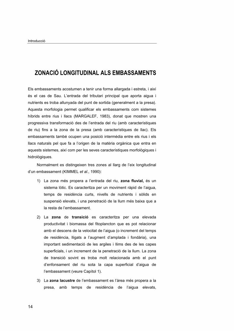
ZONACIÓ LONGITUDINAL ALS EMBASSAMENTS
Els embassaments acostumen a tenir una forma allargada i estreta, i així
és el cas de Sau. L’entrada del tributari principal que aporta aigua i
nutrients es troba allunyada del punt de sortida (generalment a la presa).
Aquesta morfologia permet qualificar els embassaments com sistemes
híbrids entre rius i llacs (MARGALEF, 1983), donat que mostren una
progressiva transformació des de l’entrada del riu (amb característiques
de riu) fins a la zona de la presa (amb característiques de llac). Els
embassaments també ocupen una posició intermèdia entre els rius i els
llacs naturals pel que fa a l’origen de la matèria orgànica que entra en
aquests sistemes, així com per les seves característiques morfològiques i
hidrològiques.
Normalment es distingeixen tres zones al llarg de l’eix longitudinal
d’un embassament (KIMMEL et al., 1990):
1) La zona més propera a l’entrada del riu, zona fluvial, és un
sistema lòtic. Es caracteritza per un moviment ràpid de l’aigua,
temps de residència curts, nivells de nutrients i sòlids en
suspensió elevats, i una penetració de la llum més baixa que a
la resta de l’embassament.
2) La zona de transició es caracteritza per una elevada
productivitat i biomassa del fitoplancton que es pot relacionar
amb el descens de la velocitat de l’aigua (o increment del temps
de residència, lligats a l’augment d’amplada i fondària), una
important sedimentació de les argiles i llims des de les capes
superficials, i un increment de la penetració de la llum. La zona
de transició sovint es troba molt relacionada amb el punt
d’enfonsament del riu sota la capa superficial d’aigua de
l’embassament (veure Capítol 1).
3) La zona lacustre de l’embassament es l’àrea més propera a la
presa, amb temps de residència de l’aigua elevats,
Introducció
15
concentracions de nutrients dissolts i partícules inorgàniques en
suspensió baixes, una major transparència de l’aigua i una capa
fòtica més fonda que a la resta de l’embassament.
Les tres zones no són unitats discretes dins de l’embassament,
altrament, són temporalment i espacialment dinàmiques. Les seves
extensions varien en funció de l’escorrentia de la conca, les
característiques dels aports (intensitat, densitat) i de la gestió que es faci
de l’embassament (fondària i cabals de sortida). Qualsevol zona pot ser
més o menys important en funció de les condicions hidrològiques. Com
que no sempre és fàcil distingir aquestes zones, alguns autors
(UHLMANN, 1991) prefereixen considerar l’embassament com un
sistema homogeni i només tenir en compte les entrades i les sortides.
Sota aquesta perspectiva, comparen el funcionament de l’embassament
amb un quemostat.
Els embassaments poden desenvolupar gradients longitudinals molt
acusats. Llavors, la condició tròfica de l’embassament canvia
gradualment de l’eutròfica a l’oligotròfica, seguint el gradient de
variacions físiques i químiques, i de processos biològics i fisiològics. Tal i
com veurem al llarg dels capítols successius, aquest és el cas de
l’embassament de Sau.
ÀREA D’ESTUDI I ANTECEDENTS
L’embassament de Sau es troba encaixat en una vall, cosa que li
confereix una morfologia llarga (18.5 km de longitud) i estreta (fondària
màxima de 84 m). Es localitza al tram mig del riu Ter, què neix als
Pirineus, a 2500 m s. n. m., i flueix al llarg de 208 km fins el Mediterrani
(SABATER et al., 1991).
Dintre de Catalunya, aquest és un embassament de capacitat
intermèdia. Això, afegit a què es troba en una regió de clima mediterrani,
fa que la hidrologia del sistema sigui molt variable entre anys. Dos dels
anys del nostre període d’estudi (1999 i 2000) van ser clarament secs
amb uns nivells de reserva d’aigua molt baixos.
Introducció
16
Sau és la primera reserva d’aigua en una cascada de tres
embassaments destinats a l'abastament d’aigua potable per a Barcelona
i la seva àrea metropolitana. La seva importància socio-econòmica
justifica que hagi estat estudiat des del primer emplenat al 1963. La sèrie
de dades de què disposem (40 anys) és la més llarga d’aquest tipus a
Espanya, recollint informació dels principals paràmetres químics i
biològics (biomasses i diversitat del fitoplancton i zooplancton). Amb tot,
el coneixement sobre l’ecologia d’aquest sistema aquàtic es fonamenta,
principalment, en dades recollides mensualment, amb perfils verticals,
dins l’àrea més propera a la presa.
Els estudis precedents descriuen Sau com un embassament
monomíctic, amb un patró anual d’estratificació tèrmica a l’estiu (des
d’abril fins a setembre) i de barreja a l’hivern (VIDAL, 1977). Alguns
aspectes de l’estructura tèrmica i dels patrons de circulació interna han
estat recentment estudiats (HAN et al., 2000), aplicant un model de
simulació hidrodinàmica (1D, DYRESM). Les simulacions han demostrat
la gran influència del riu Ter a l’estructura tèrmica a Sau. També s’ha
demostrat que l’efecte del temps de residència sobre l’estructura tèrmica
es manifesta en canvis a la fondària de la termoclina.
El procés d’eutrofització que ha patit l’embassament de Sau, des de
1963 fins 1990, també es troba ben documentat (VIDAL, 1977; VIDAL,
1993; ARMENGOL i VIDAL, 1988; ARMENGOL et al., 1994). A partir de
1991, es van construir i posar en funcionament diverses estacions
depuradores d’aigües residuals a la part alta de la conca del Ter.
Aquestes depuradores, en un principi, només disposaven de tractaments
físico-químics. Aquest tipus de tractaments retiren el fòsfor dissolt de
l’aigua força eficaçment, cosa que va provocar el descens de les
càrregues d’aquest nutrient a l’embassament a partir del 1994. Fins a la
implantació de tractaments biològics addicionals (1998) no es va apreciar
una disminució de les càrregues de nitrogen. Tot i la reducció de
l’entrada de nutrients, les dades recents mostren que les concentracions
de clorofil·la a a l’embassament de Sau continuen sent pròpies de
sistemes eutròfics (MASON, 1996). No es descarta una milloria en
l’estrat tròfic de Sau en el futur. La recollida de dades endegada al 1963
continua efectuant-se mensualment.
Introducció
17
En els estudis previs de l’ecologia del plancton a Sau, la comunitat
microbiana no es va considerar. Aquests estudis es centraven en la
taxonomia, i en les mesures de biomassa del fitoplancton i el
zooplancton. La metodologia indicada per al fito- i zooplancton no era
l’apropiada pels components microbians del plancton per diversos
motius:
- es recollia les mostres amb xarxes que permeten el pas dels
bacteris, els flagel·lats i la majoria de ciliats (53 µm∅);
- s’utilitzava fixadors extremadament agressius pels flagel·lats i
ciliats, que resultaven en cèl·lules que no es podien
reconèixer;
- les pressions aplicades a la filtració (>20mm Hg) de les
mostres eren massa elevades pels protistes, provocant el
trencament de les cel·lules;
- els augments de la microscopia òptica per enumerar fito- i
zooplankton eren massa baixos per poder detectar els
microorganismes.
Tan sols un projecte d’estudi dirigit a les poblacions microbianes es
va dur a terme a l’agost de 1994. D’aquest treball es va publicar un
article sobre la presència de virus de mida gran a l’embassament de Sau
(SOMMARUGA et al., 1995). Desprès d’aquest treball es van obrir noves
qüestions sobre l’ecologia de l’embassament, principalment pel que fa a
la microbiologia i l’heterogeneïtat longitudinal (no tractada fins llavors en
termes d’ecologia microbiana). Podem dir que va ser l’origen del present
estudi. Així, vaig començar la tesi doctoral al gener de 1997, assumint
l’estudi de l’ecologia microbiana a l’embassament de Sau. El Dr. Karel
Šimek, que col·labora amb el nostre grup des de 1994, em va introduir en
aquesta àrea i em va ensenyar la metodologia adequada.
Introducció
18
OBJECTIUS DEL PRESENT ESTUDI
Fins l’any 1996, pocs estudis s’havien dut a terme a Sau sobre els
micoorganismes planctònics i el seu paper en l’ecologia de
l’embassament, tot i que molts altres aspectes d’aquest sistema es
coneixien àmpliament. L’objectiu principal que ens vam marcar per la
present tesi pretenia caracteritzar la xarxa tròfica microbiana d’aquest
ecosistema eutròfic, amb elevades aportacions de carboni orgànic
al·locton.
En primer lloc, volíem conèixer els rangs d’abundància i tenir una
aproximació a la composició específica de bacteris i protistes (flagel·lats
heteròtrofs i ciliats) a l’epilimnion de l’embassament. El nostre treball
també es va centrar en l’estudi de les activitats microbianes: producció
bacteriana i taxes de bacterivoria dels protozous.
Vam descobrir una marcada heterogeneïtat espacial en els
paràmetres físics, químics i biològics des de el riu fins a la presa; pel que
es va posar una atenció especial a aquests gradients. Volíem arribar a
descriure les forces que controlaven la zonació longitudinal al llarg de
l’embassament.
Desprès de 5 anys d’estudi (1996-2000), vam ser capaços d’avaluar
la contribució de la xarxa microbiana pelàgica dins de l’embassament
com a font de carboni per a nivells tròfics superiors.
Els resultats d’aquest treball es presenten en sis capítols. Cadascun
ha estat escrit con un article independent, centrat en un tema particular
amb la seva introducció i la seva discussió. Alguns d’ells estan publicats i
altres estan en procés de publicació. He estat afortunada de que el
nostre grup de treball hagi estat molt actiu durant el període 1996-2000,
duent a terme moltes col·laboracions amb altres científics que han donat
com a resultat una bona quantitat de publicacions a les que apareix-ho
com coautora. En aquest treball, però, només es presenten els resultats
que he processat personalment per tal d’assolir els objectius proposats.
Les publicacions produïdes pel nostre grup han estat incloses com a
Introducció
19
comentaris, amb les seves cites bibliogràfiques corresponents, per tal
d’aclarir les qüestions relacionades amb la xarxa tròfica microbiana.
Els capítols han estat ordenats de manera lògica, començant per
les principals forces en el control de la xarxa tròfica microbiana e
introduint-hi qüestions més específiques relacionades amb les diferents
particularitats en aquest embassament (els components més comuns i la
seva activitat a l’epilimnion). Els objectiu específics en cada capítol es
resumeixen a continuació:
- Capítol 1. Es fa una descripció de les principals forces físiques
que actuen en l’eix longitudinal de l’embassament. L’objectiu va
ser caracteritzar la variació estacional en el patró de circulació al
llarg de l’embassament.
- Capítol 2. S’examinen els gradients químics longitudinals i la seva
variació en funció de les condicions físiques. L’objectiu principal
va ser aclarir la importància dels elevats aports al·lòctons de
nutrients en la composició química de l’epilimnion, i com aquests
nutrients són processats al llarg de l’embassament.
- Capítol 3. Es mostra un transecte longitudinal amb clars gradients
en les activitats biològiques. Es descriu amb detall com els
diferents grups d’organismes planctònics es desenvolupen
seqüencialment a partir dels aports que fa el riu.
- Capítol 4. S’agrupen els diferents transectes per el seu estudi
integrat. Es descriuen els patrons generals de distribució i les
activitats microbianes en aquest embassament. També es
detallen la diversitat i les activitats especifiques dels principals
components del plancton microbià.
- Capítol 5. Es fa una recapitulació de tots els resultats en termes
de biomassa i producció i es prova de donar una visió general
dels fluxos de carboni en el context d’una successió longitudinal
de la comunitat pelàgica. L’objectiu d’aquest estudi va ser avaluar
la importància de la xarxa tròfica microbiana a Sau.
- Capítol 6. Es comparen les taxes específiques de creixentment
dels nanoflagel·lats heteròtrofs i dels ciliats en un experiment amb
Introducció
20
microcosmos. L’objectiu va ser conèixer aquestes taxes de
creixement i comprovar si la xarxa tròfica microbiana es troba
regulada per la depredació del zooplancton o per la disponibilitat
de recursos.
INTRODUCTION

Introduction
23
THE MICROBIAL FOOD WEB:COMPONENTS AND THEIR IMPORTANCE
IN THE PELAGIC FOOD WEB
The classical view of the trophic functioning of the planktonic food
chain is the autotrophic production of organic material by phytoplankton is
consumed by zooplankton, which in turn is consumed by fish. While the
size and the productivity of these large body organisms were natural
elements in aquatic studies under this view, microorganisms were not
integrated into the analysis of whole ecosystems. POMEROY (1974)
challenged this point of view by proposing an alternative paradigm for the
marine pelagic food web. He argued that microorganisms, whose
biomass is approximately equal to that of the traditional “net” plankton,
were potentially greater movers of energy and materials because of their
higher metabolic rates. The “microbial loop” concept soon appeared
(AZAM et al., 1983). Initially the loop was believed to consist of bacteria,
phagotrophic flagellates and other protozoans, such as ciliates, and
based primarily on organic exudates of the phytoplankton. In this loop,
bacterial carbon content would flow to zooplankton in successive
predation steps of flagellates on bacteria, of ciliates on flagellates, and of
zooplankton on flagellates and ciliates, thus reaching the classical food
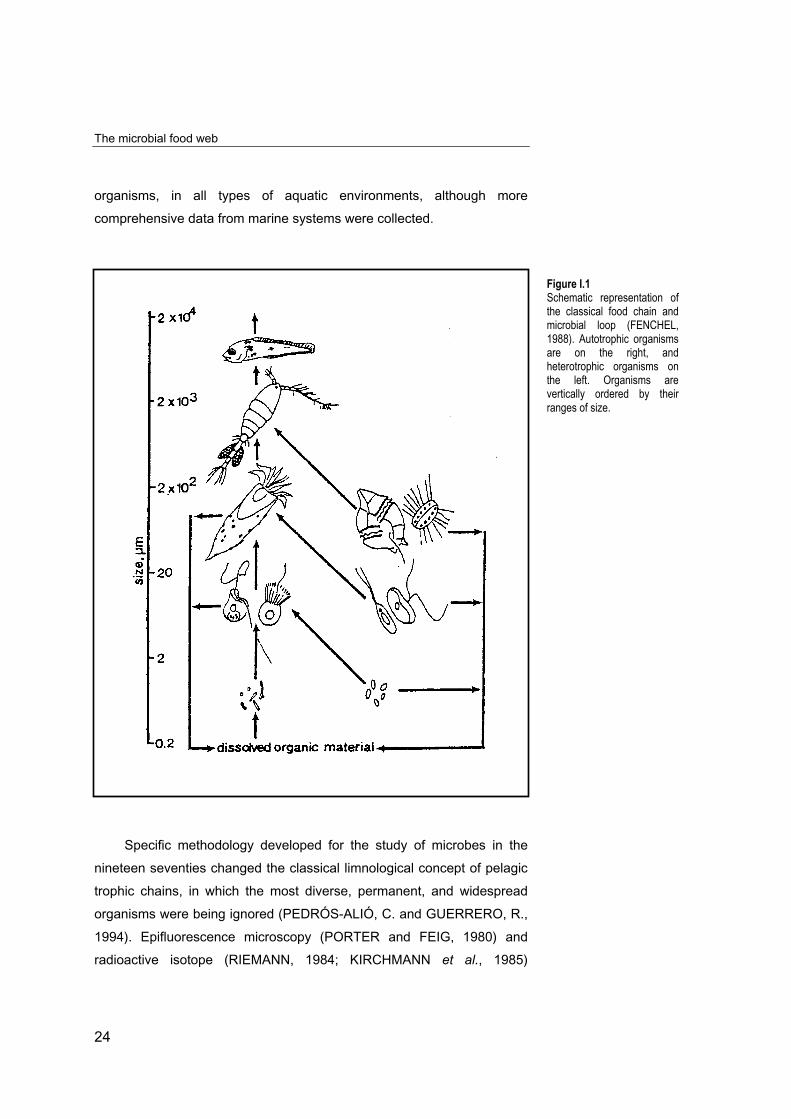
chain (Fig. I.1). These arguments were equally valid for freshwaters,
which possess the same fundamental planktonic structure. In this way,
PORTER et al. (1979) and SHERR and SHERR (1988) point out the role
of protozoans as links in freshwater planktonic food chains, representing
an important mechanism by which dissolved organic matter (DOC),
particulated organic matter (POC) and bacteria enter planktonic food
chains.
In studies from 1980 to 1995, increasing attention was paid to the
occurrence, taxonomy and functional role of the microbial plankton
The microbial food web
24
organisms, in all types of aquatic environments, although more
comprehensive data from marine systems were collected.
Specific methodology developed for the study of microbes in the
nineteen seventies changed the classical limnological concept of pelagic
trophic chains, in which the most diverse, permanent, and widespread
organisms were being ignored (PEDRÓS-ALIÓ, C. and GUERRERO, R.,
1994). Epifluorescence microscopy (PORTER and FEIG, 1980) and
radioactive isotope (RIEMANN, 1984; KIRCHMANN et al., 1985)
Figure I.1Schematic representation ofthe classical food chain andmicrobial loop (FENCHEL,1988). Autotrophic organismsare on the right, andheterotrophic organisms onthe left. Organisms arevertically ordered by theirranges of size.
Introduction
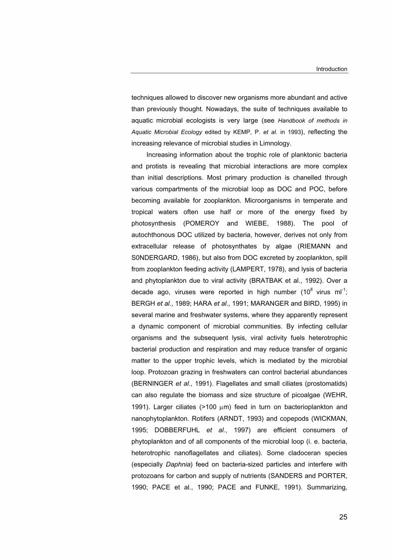
25
techniques allowed to discover new organisms more abundant and active
than previously thought. Nowadays, the suite of techniques available to
aquatic microbial ecologists is very large (see Handbook of methods in
Aquatic Microbial Ecology edited by KEMP, P. et al. in 1993), reflecting the
increasing relevance of microbial studies in Limnology.
Increasing information about the trophic role of planktonic bacteria
and protists is revealing that microbial interactions are more complex
than initial descriptions. Most primary production is chanelled through
various compartments of the microbial loop as DOC and POC, before
becoming available for zooplankton. Microorganisms in temperate and
tropical waters often use half or more of the energy fixed by
photosynthesis (POMEROY and WIEBE, 1988). The pool of
autochthonous DOC utilized by bacteria, however, derives not only from
extracellular release of photosynthates by algae (RIEMANN and
S0NDERGARD, 1986), but also from DOC excreted by zooplankton, spill
from zooplankton feeding activity (LAMPERT, 1978), and lysis of bacteria
and phytoplankton due to viral activity (BRATBAK et al., 1992). Over a
decade ago, viruses were reported in high number (108 virus ml-1;
BERGH et al., 1989; HARA et al., 1991; MARANGER and BIRD, 1995) in
several marine and freshwater systems, where they apparently represent
a dynamic component of microbial communities. By infecting cellular
organisms and the subsequent lysis, viral activity fuels heterotrophic
bacterial production and respiration and may reduce transfer of organic
matter to the upper trophic levels, which is mediated by the microbial
loop. Protozoan grazing in freshwaters can control bacterial abundances
(BERNINGER et al., 1991). Flagellates and small ciliates (prostomatids)
can also regulate the biomass and size structure of picoalgae (WEHR,
1991). Larger ciliates (>100 µm) feed in turn on bacterioplankton and
nanophytoplankton. Rotifers (ARNDT, 1993) and copepods (WICKMAN,
1995; DOBBERFUHL et al., 1997) are efficient consumers of
phytoplankton and of all components of the microbial loop (i. e. bacteria,
heterotrophic nanoflagellates and ciliates). Some cladoceran species
(especially Daphnia) feed on bacteria-sized particles and interfere with
protozoans for carbon and supply of nutrients (SANDERS and PORTER,
1990; PACE et al., 1990; PACE and FUNKE, 1991). Summarizing,
The microbial food web
26
bacteria and their consumers can exert both direct and indirect effects on
trophic relations, as they are supplemental food resources, competitors,
and predators, at all levels of the classic food chain. Therefore,
consumers of bacterial production can exert top-down and lateral, as well
as bottom-up control (PORTER, 1996). The microbial loop concept has
changed from “orderly level transfers of nutrients and energy from
bacteria to metazoans” to a “complex trophic web”. The microbial loop is
a component and integral part of a larger microbial food web (SHERR
and SHERR, 1988) which includes all pro- and eucaryotic unicellular
organisms, both autotrophic and heterotrophic, and all are integrated in a
general planktonic food web (PORTER, 1996). This web concept is
represented in Figure I.2.
It has been established that microbes play a key role in nutrient
cycling and energy flows in aquatic ecosystems. Typical abundances of
Figure I.2The contemporary view ofmicrobial food web structure(below the dotted line) inrelation to the classic foodchain (above the dotted line)in the pelagic zone of lakes(from WEISSE andSTOCKNER, 1992). Boxesare vertically ordered byranges of size of theorganisms. Full lines andarrows indicate feedinginteractions, broken lines andarrows, viral infection. Thepool of dissolved organicmatter is replenished byvarious release processes(excretion, exudation, celllysis, sloppy feeding) fromeach compartment and usedas substrate by bacteria.
Introduction
27
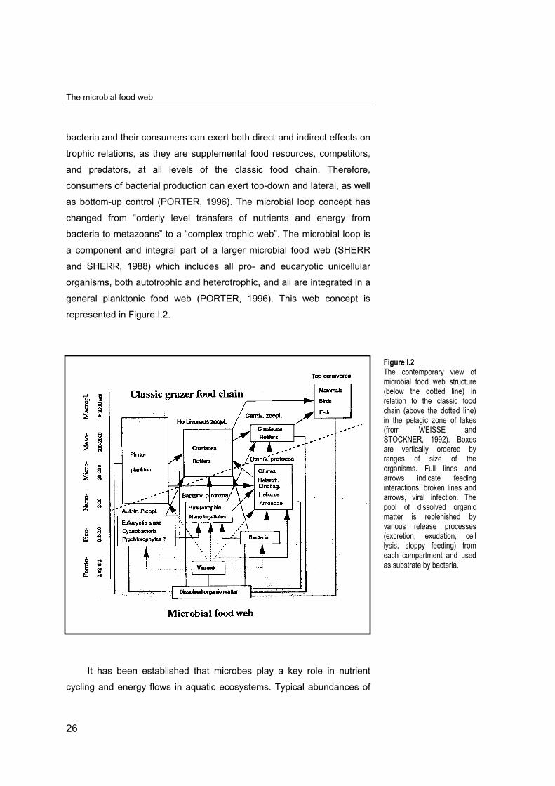
main groups (i. e. picoalgae, viruses, bacteria, HNF and ciliates) in
oligotrophic and eutrophic lakes are summarized in Table I.1. The
ecological constraints on the functioning of microbial communities include
a variety of interactions that differ in intensity over time and space, see
RIEMANN and CHRISTOFFERSEN (1993) and references listed therein.
Abundances of main groups of microbial plankton
oligotrophic lakes eutrophic lakes
Picoalgae 104 ml-1
(8% of the total chlorophyll)>106 ml-1
(1% of the total chlorophyll)
Viruses 106 ml-1 > 108 ml-1
Bacteria 105 ml-1 107 ml-1
HNF 102 ml-1 105 ml-1
Ciliates 10 ml-1 103 ml-1
WEISSE et al. (1990) described in mesotrophic Lake Constance the
importance of microbial loop during early phytoplankton blooms. During
clear water phase in the mesotrophic Římov Reservoir (ŠIMEK and
STRAŠKRABOVÁ) protozoans decreased significantly, and thus their
role in bacterivory was negligible. NIXDORF and ARNDT (1993)
described a shift within the metabolic interactions of the microbial food
web from winter/spring to summer, indicating a high significance of the
protozooplankton as a regulator on bacteria during the colder season,
whereas from early summer the influence of metazooplankton dominated
by cladocerans was evident in the eutrophic Lake Müggelsee. During
massive bloom of cyanobacteria in eutrophic shallow lake,
CHRISTOFFERSEN et al. (1990) found that microzooplankton and
metazooplankton were more important than HNF in controlling the
bacterial production. There are, however, other examples where the role
of ciliates in the carbon budgets is minor (PACE et al., 1990). The trophic
state of the system is high important to explain these differences between
systems. As an example, ŠIMEK et al. (1999) described that ciliates
Table I.1Abundances of main groupsof microbial plankton in lakesdepending on degree oftrophy. From RIEMANN andCHRISTOFFERSEN (1993)and references listed therein,excepting viruses (from HARAet al., 1991 and SOMMA-RUGA et al., 1995).
The microbial food web
28
become as bacterivores as HNF with increasing trophy of three reservoirs
studied.
It is still under discussion, however, what relevance do
microorganisms and their interactions have along the gradient of lakes of
different trophy (WEISSE, 1991; WEISSE and STOCKNER, 1993; Del
GIORGIO and GASOL, 1995). Although the abundance of
microorganisms increases with higher nutrient load and primary
production (Table I.1), it is believed that the relative contribution of the
microbial food web to the carbon flux decreases along eutrophication
gradients. But RIEMANN and CHRISTOFFERSEN (1993) in their
analysis of the microbial loop along an increasing productivity gradient
suggested increasing importance compared to the classical grazer food
chain.
In order to evaluate the importance of microbial food web in the Sau
Reservoir our group of research purposed to measure abundances and
activities of microbes as well as phytoplankton and zooplankton. This
thesis forms part of a general project, considering autotrophic processes
in the epilimnion of the Sau Reservoir, and their connection with the
heterotrophic activities, summarised in this study. Consequently, the
study focuses on the epilimnetic community. More attention has been
paid to horizontal gradients in the reservoir rather than vertical
heterogeneity. In addition, the complex methodology for sample
processing required by summer hypolimnetic samples of anaerobic
conditions, is another reason.
SPATIAL HETEROGENEITY IN RESERVOIRS,LONGITUDINAL ZONATION
Reservoirs, such as the Sau Reservoir, are often large and narrow,
receiving water and nutrient inputs from a single large tributary, which is
distant from the point of discharge. These characteristics allows to define
Introduction
29
reservoirs as hybrid systems between rivers and lakes (MARGALEF,
1983), because they exhibit a progressive transformation from lotic
systems (river inflow) to lake systems (nearer the dam). Reservoirs also
occupy an intermediate position between rivers and natural lakes in
regard to their organic matter sources, as well as their morphologic and
hydrodynamic characteristics.
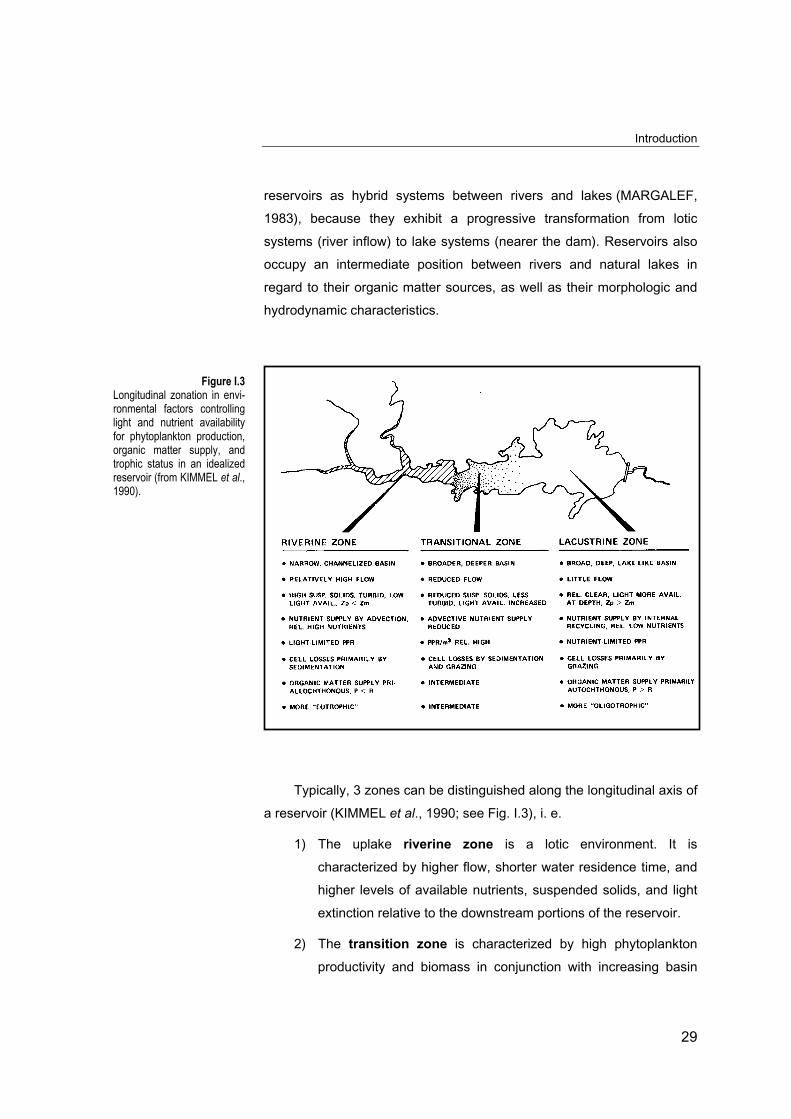
Typically, 3 zones can be distinguished along the longitudinal axis of
a reservoir (KIMMEL et al., 1990; see Fig. I.3), i. e.
1) The uplake riverine zone is a lotic environment. It is
characterized by higher flow, shorter water residence time, and
higher levels of available nutrients, suspended solids, and light
extinction relative to the downstream portions of the reservoir.
2) The transition zone is characterized by high phytoplankton
productivity and biomass in conjunction with increasing basin
Figure I.3Longitudinal zonation in envi-ronmental factors controllinglight and nutrient availabilityfor phytoplankton production,organic matter supply, andtrophic status in an idealizedreservoir (from KIMMEL et al.,1990).
Spatial heterogeneity in reservoirs
30
breadth, decreasing flow velocity, increased water residence
time, large sedimentation of silt and clay particles from near-
surface waters, and increased light penetration. The transition
zone is often associated with the plunge point (see Chapter 1),
where the river inflow plunge beneath the water surface.
3) The lacustrine zone of the reservoir is an area near the dam,
with usually longer water residence time, lower concentration of
dissolved nutrients and suspended inorganic particles, higher
water transparency, and a deeper photic layer than other areas
of the reservoir.
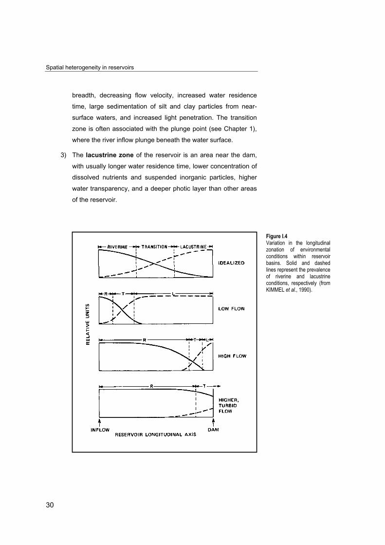
Figure I.4Variation in the longitudinalzonation of environmentalconditions within reservoirbasins. Solid and dashedlines represent the prevalenceof riverine and lacustrineconditions, respectively (fromKIMMEL et al., 1990).
Introduction
31
The three zones are not discrete units in the reservoir, but spatially
and temporally dynamic. Their area fluctuates in response to watershed
runoff, inflow characteristics, density flow behaviour, and reservoir
operations (Fig. I.4). Any zone takes more or less importance depending
on hydrological conditions. Because are not always easily
distinguishable, some authors (e. g. UHLMANN, 1991) prefer to consider
reservoirs as a homogeneous system, taking in consideration only inflows
and outflows. This school of thought compares reservoir functioning to a
chemostat.
Marked longitudinal gradients may develop in reservoirs. Then,
trophic state gradually changes from eutrophic to oligotrophic conditions
down the gradient owing to physical, chemical and biological-
physiological processes. It is the case of the Sau Reservoir, due to its
special morphology, long and narrow, as we will see in the following
section.
STUDY SITE AND STATE OF THE ART
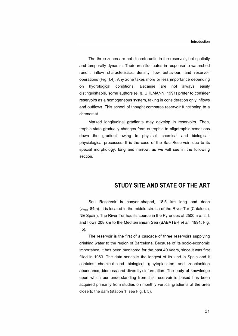
Sau Reservoir is canyon-shaped, 18.5 km long and deep
(zmax=84m). It is located in the middle stretch of the River Ter (Catalonia,
NE Spain). The River Ter has its source in the Pyrenees at 2500m a. s. l.
and flows 208 km to the Mediterranean Sea (SABATER et al., 1991; Fig.
I.5).
The reservoir is the first of a cascade of three reservoirs supplying
drinking water to the region of Barcelona. Because of its socio-economic
importance, it has been monitored for the past 40 years, since it was first
filled in 1963. The data series is the longest of its kind in Spain and it
contains chemical and biological (phytoplankton and zooplankton
abundance, biomass and diversity) information. The body of knowledge
upon which our understanding from this reservoir is based has been
acquired primarily from studies on monthly vertical gradients at the area
close to the dam (station 1, see Fig. I. 5).
Study site and state of the art
32
In Catalonia, this is a reservoir of intermediate capacity and highly
variable in its hydrology between years, due to the Mediterranean climate
Figure I.5Study location in Spain(upper) map. Location of theRiver Ter and the Sau Re-servoir in Catalonia (middlemap). Location of the ninesampling stations along thelongitudinal axis of thereservoir (bottom map).
SPAIN
FRANCE
0 200 km100MEDITERRANEAN S
EA
PO
RT
UG
AL
Catalonia60 km0 30
THE SAU RESERVOIR
19
8
7
6
5
4
3
2
Sampling stationsn
river
dam
2 km0 1
Introduction
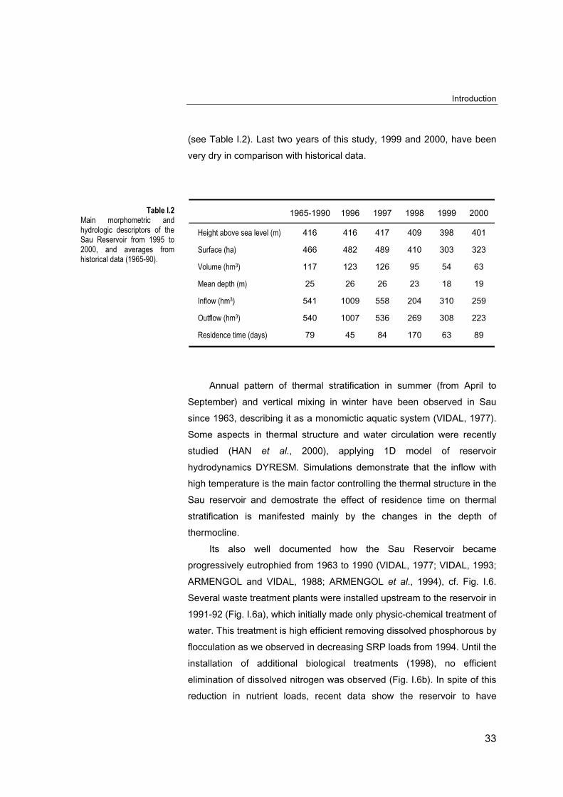
33
(see Table I.2). Last two years of this study, 1999 and 2000, have been
very dry in comparison with historical data.
1965-1990 1996 1997 1998 1999 2000
Height above sea level (m) 416 416 417 409 398 401
Surface (ha) 466 482 489 410 303 323
Volume (hm3) 117 123 126 95 54 63
Mean depth (m) 25 26 26 23 18 19
Inflow (hm3) 541 1009 558 204 310 259
Outflow (hm3) 540 1007 536 269 308 223
Residence time (days) 79 45 84 170 63 89
Annual pattern of thermal stratification in summer (from April to
September) and vertical mixing in winter have been observed in Sau
since 1963, describing it as a monomictic aquatic system (VIDAL, 1977).
Some aspects in thermal structure and water circulation were recently
studied (HAN et al., 2000), applying 1D model of reservoir
hydrodynamics DYRESM. Simulations demonstrate that the inflow with
high temperature is the main factor controlling the thermal structure in the
Sau reservoir and demostrate the effect of residence time on thermal
stratification is manifested mainly by the changes in the depth of
thermocline.
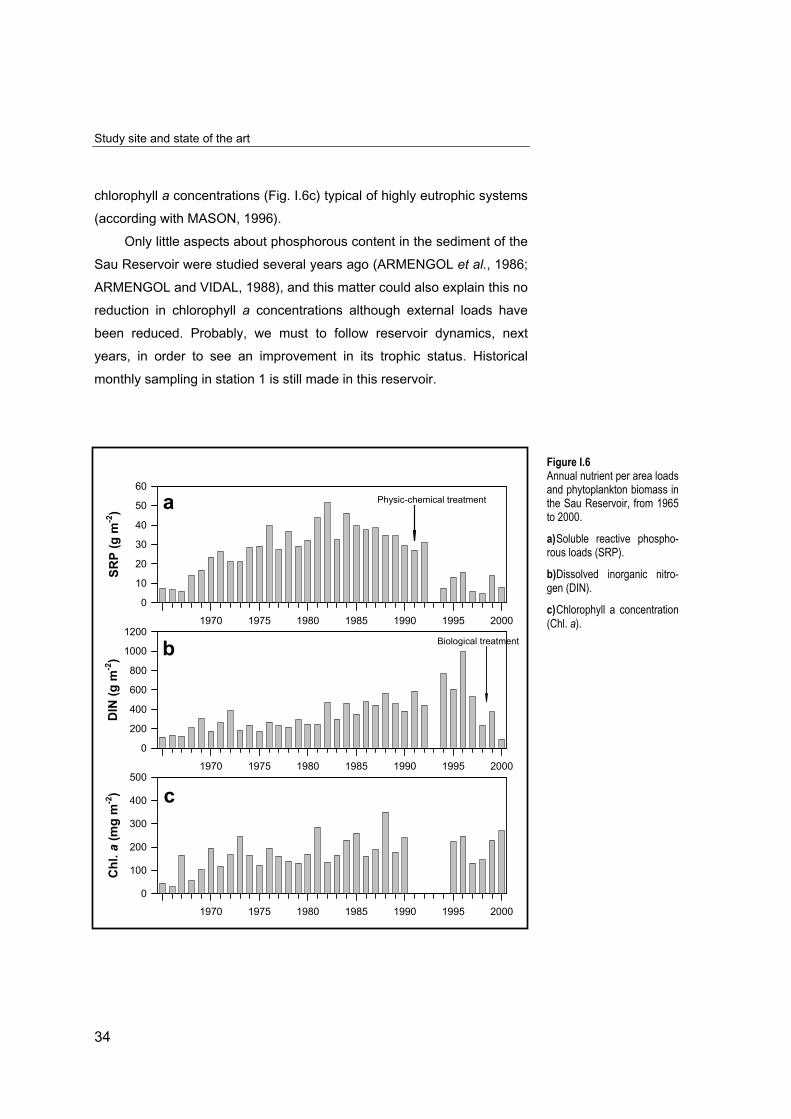
Its also well documented how the Sau Reservoir became
progressively eutrophied from 1963 to 1990 (VIDAL, 1977; VIDAL, 1993;
ARMENGOL and VIDAL, 1988; ARMENGOL et al., 1994), cf. Fig. I.6.
Several waste treatment plants were installed upstream to the reservoir in
1991-92 (Fig. I.6a), which initially made only physic-chemical treatment of
water. This treatment is high efficient removing dissolved phosphorous by
flocculation as we observed in decreasing SRP loads from 1994. Until the
installation of additional biological treatments (1998), no efficient
elimination of dissolved nitrogen was observed (Fig. I.6b). In spite of this
reduction in nutrient loads, recent data show the reservoir to have
Table I.2Main morphometric andhydrologic descriptors of theSau Reservoir from 1995 to2000, and averages fromhistorical data (1965-90).
Study site and state of the art
34
chlorophyll a concentrations (Fig. I.6c) typical of highly eutrophic systems
(according with MASON, 1996).
Only little aspects about phosphorous content in the sediment of the
Sau Reservoir were studied several years ago (ARMENGOL et al., 1986;
ARMENGOL and VIDAL, 1988), and this matter could also explain this no
reduction in chlorophyll a concentrations although external loads have
been reduced. Probably, we must to follow reservoir dynamics, next
years, in order to see an improvement in its trophic status. Historical
monthly sampling in station 1 is still made in this reservoir.
Figure I.6Annual nutrient per area loadsand phytoplankton biomass inthe Sau Reservoir, from 1965to 2000.
a) Soluble reactive phospho-rous loads (SRP).
b) Dissolved inorganic nitro-gen (DIN).
c) Chlorophyll a concentration(Chl. a).1970 1975 1980 1985 1990 1995 2000
SR
P (
g m
-2)
0
10
20
30
40
50
60
1970 1975 1980 1985 1990 1995 2000
DIN
(g
m-2
)
0
200
400
600
800
1000
1200
1970 1975 1980 1985 1990 1995 2000
Ch
l. a
(m
g m
-2)
0
100
200
300
400
500
Physic-chemical treatment
Biological treatmentb
c
a
Introduction
35
Historically, in studies of plankton ecology from the Sau Reservoir,
microbial communities have been ignored. Most studies on the plankton
community have focused on the taxonomy and biomass determinations
of phyto- and zooplankton. Microbial plankton groups have been
overlooked in studies from Sau due to the methodology used for both
phytoplankton and zooplankton samples:
- to sample (p.e. nets through which bacteria, flagellates and
most ciliates pass, 53µm∅),
- to preserve (extremely disruptive to flagellates and ciliates,
and render their cells unrecognisable),
- to filtrate (microbial groups are very sensitive to pressures
>20mm Hg)
- and to enumerate (low optical magnifications).
Only one microbiological project was conducted in August 1994,
when several scientists meet in this reservoir. They published a paper
about the presence of large virus-like particles in the Sau (SOMMARUGA
et al., 1995). From that sampling new questions about ecology of Sau
where constructed, mainly on microbiological point of view and following
longitudinal heterogeneity (not described until then in terms of microbial
ecology). We could say that it was the origin of the present study.
I started my PhD in January 1997, assuming a new area of study
and methodology in the Sau Reservoir, the microbial ecology. I was
helped by Dr. Karel Šimek, who has collaborated with our group of
research since 1994.
To study longitudinal changes in chemistry and biology along the
main axis of the reservoir, nine sampling stations were established for the
present study at ca. 1.8 km intervals (see Fig. I. 5).
Objectives of this study
36
OBJECTIVES OF THIS STUDY
Although many aspects about ecosystem have been extensively
studied until 1996 in this warm, eutrophic and monomictic reservoir, as
yet relatively little studies have been conducted about protozoan
components of the plankton and their role in this system. The main
objective was to characterize microbial food web in this eutrophic
ecosystem, with high organic allocthonous inputs.
First we would know ranged abundances and specific composition
of bacteria and protozoa (hetrotrophic nanoflagellates and ciliates) in the
epilimnion of the Sau Reservoir. We also focused our study in microbial
activities: bacterial production and grazing rates on bacteria by protozoa.
We discovered a marked spatial heterogeneity in chemical, physical
and biotic parameters from the river inflow to the dam; and we paid more
attention to these gradients. Then we wanted to describe main forces
controlling longitudinal zonation through the reservoir.
From five years of study (1996-2000), we were able to evaluate the
contribution of pelagic microbial food web in the reservoir, as a carbon
flow and a source to higher trophic levels (zooplankton, fishes).
Results from this study are presented in six chapters. Each chapter
has been written as an independent article focused on a particular topic
with its own introduction and discussion. Some of them are published in
one or several papers and other are submitted or in press. I have been
lucky that our group of research has been very active in the 1996-2000
period, making several collaborations with other scientists resulting in
high amount of published papers in which I am co-author. Nevertheless, I
have summarized in this thesis only the data directly processed by me
following my own objectives. The papers published by our group have
been introduced as comments (with its quotations) to understand all
questions related to microbial food web.
Introduction
37
The chapters have been arranged following a logical order, starting
in major forces controlling microbial food web and introducing more
specific questions related to its particularity in this reservoir (common
components and their activity in the epilimnion). The main objectives of
each chapter are summarized as follows:
- Chapter 1 is a description of the main physical forces acting in the
longitudinal axis of the reservoir. The objective of this section was
to characterize seasonal variation in circulation patterns through
the reservoir.
- Chapter 2 examines chemical longitudinal gradients and its
variation depending on physical conditions. The main objective
was to elucidate the relevance of high allochthonous nutrient
inputs on the epilimnion chemical water composition of the
reservoir and how they are processed from the river to the dam.
- Chapter 3 shows a clear longitudinal transect in the epilimnion
where high gradients in biological activity were found. This study
describes in detail how planktonic groups develop from the source
of river inputs.
- Chapter 4 gathers up all longitudinal transects under a general
point of view, describing general patterns and specific microbial
activities in this reservoir. Diversity and species-specific activities
of the main components in microbial plankton are also detailed.
- Chapter 5 is a summary of all data in terms of biomass and
production, and attempts to give an overall view on the carbon
fluxes within the context of longitudinal pelagic community
succession. The objective of this study was to evaluate the
importance of microbial food web in the Sau Reservoir.
- Chapter 6 compares heterotrophic nanoflagellates and specific
ciliate growth rates calculated in a microcosm experiment. Our

Objectives of this study
38
goal was to know these growth rates and to test top-down control
versus bottom-up control on microbial food web.
MATERIAL AND METHODS

Material and methods
41
SAMPLINGS
In order to study physical, chemical and biological longitudinal
gradients in the Sau Reservoir, nine sampling points were stablished
from the river inflow to the dam. At every point station (see Figure I.1) we
made a profile from the surface to the bottom with a multiparametric
probe and collected integrated water samples from the epilimnion for
chemical and biological analysis. Usually we spent two or three days
sampling, but ever we took water samples more quickly than water
moved through the reservoir.
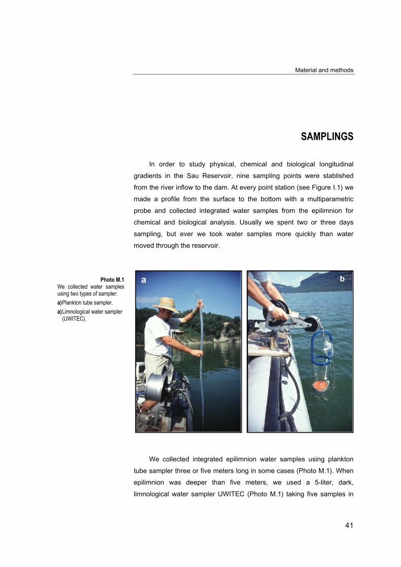
We collected integrated epilimnion water samples using plankton
tube sampler three or five meters long in some cases (Photo M.1). When
epilimnion was deeper than five meters, we used a 5-liter, dark,
limnological water sampler UWITEC (Photo M.1) taking five samples in
a bPhoto M.1We collected water samplesusing two types of sampler:a) Plankton tube sampler.a) Limnological water sampler
(UWITEC).
Physical and chemical parameters
42
several depths and mixing them in a 25-liter, dark, polyethylene bottle.
The water was stored in 5-liter or 25-liter, dark, polyethylene bottles
awaiting analyses.
PHYSICAL AND CHEMICAL PARAMETERS
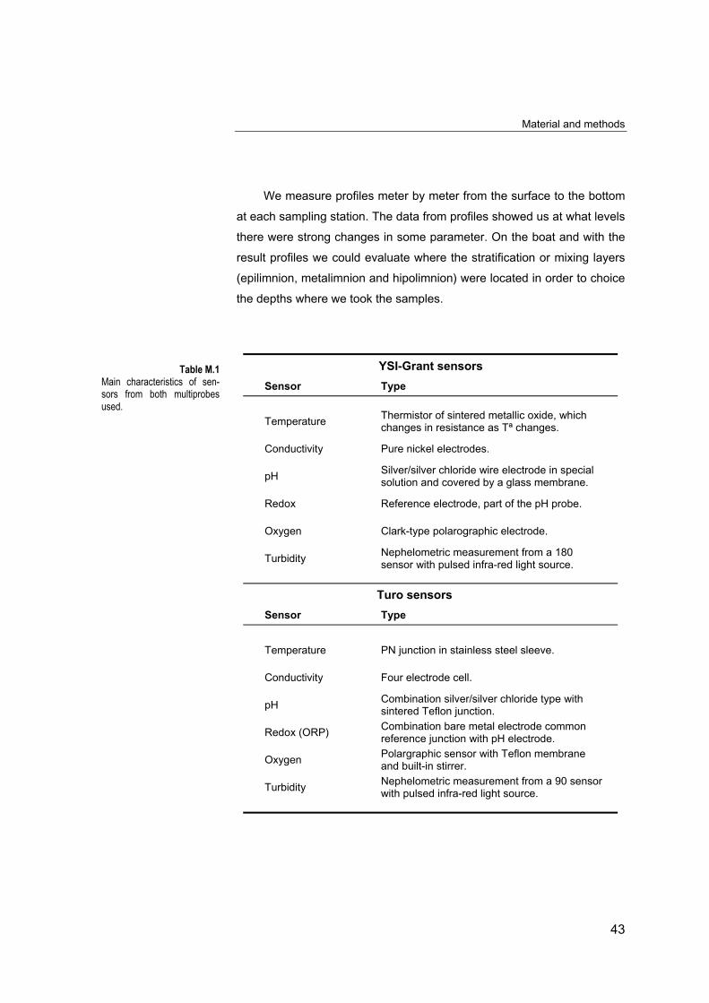
Temperature, conductivity, pH, redox, oxygen and turbidity
We measured temperature (ºC), conductivity (µS cm-2), pH, redox
(mV), oxygen saturation percentage, oxygen concentration (mg l-1) and
nephelometric turbidity (ntu) using two kinds of multiprobe provided both
with a cable 100 meters long.
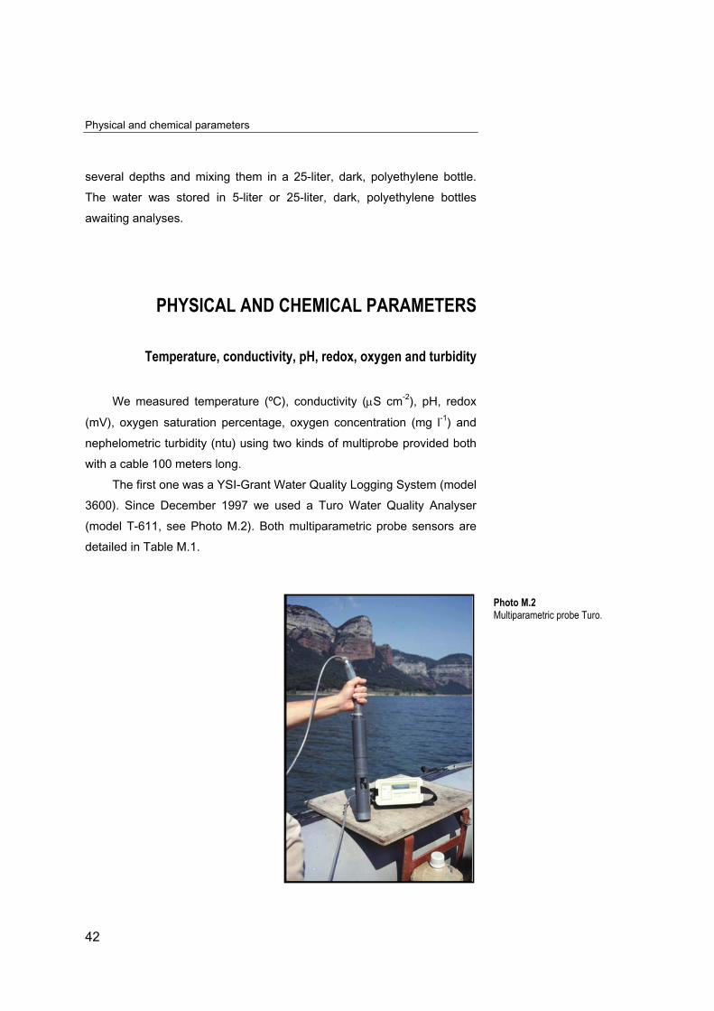
The first one was a YSI-Grant Water Quality Logging System (model
3600). Since December 1997 we used a Turo Water Quality Analyser
(model T-611, see Photo M.2). Both multiparametric probe sensors are
detailed in Table M.1.
Photo M.2Multiparametric probe Turo.
Material and methods
43
We measure profiles meter by meter from the surface to the bottom
at each sampling station. The data from profiles showed us at what levels
there were strong changes in some parameter. On the boat and with the
result profiles we could evaluate where the stratification or mixing layers
(epilimnion, metalimnion and hipolimnion) were located in order to choice
the depths where we took the samples.
YSI-Grant sensors
Sensor Type
TemperatureThermistor of sintered metallic oxide, whichchanges in resistance as Tª changes.
Conductivity Pure nickel electrodes.
pHSilver/silver chloride wire electrode in specialsolution and covered by a glass membrane.
Redox Reference electrode, part of the pH probe.
Oxygen Clark-type polarographic electrode.
TurbidityNephelometric measurement from a 180sensor with pulsed infra-red light source.
Turo sensors
Sensor Type
Temperature PN junction in stainless steel sleeve.
Conductivity Four electrode cell.
pHCombination silver/silver chloride type withsintered Teflon junction.
Redox (ORP)Combination bare metal electrode commonreference junction with pH electrode.
OxygenPolargraphic sensor with Teflon membraneand built-in stirrer.
TurbidityNephelometric measurement from a 90 sensorwith pulsed infra-red light source.
Table M.1Main characteristics of sen-sors from both multiprobesused.
Physical and chemical parameters
44
Secchi depth
We used 30cm diameter, and black-white dish to measure the
Secchi depth (cm).
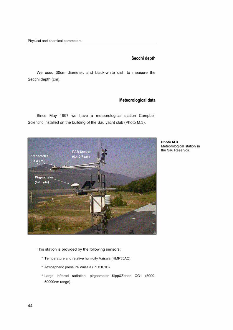
Meteorological data
Since May 1997 we have a meteorological station Campbell
Scientific installed on the building of the Sau yacht club (Photo M.3).
This station is provided by the following sensors:
° Temperature and relative humidity Vaisala (HMP35AC).
° Atmospheric pressure Vaisala (PTB101B).
° Large infrared radiation: pirgeometer Kipp&Zonen CG1 (5000-
50000nm range).
Photo M.3Meteorological station inthe Sau Reservoir.
Material and methods
45
° Sun radiation: piranometer Kipp&Zonen CM3 (300-3000nm range).
° Photosynthetic active radiation (PAR): Skye SKP215 (400-700nm
range).
° Anemometer –weather vane (RM Young 05103).
° Rain gauge (Munro R102).
Chemical analyses
Total particulate nitrogen and carbon were measured via
elemental analysis in a 1500 Carlo Erba analyser. Vanadium pentaoxid is
used as catalyst. Specific volume of sample is filtered through
precombusted Whatman GF/F glass microfibre filter (24mm ∅) which is
analysed.
Particulate material (PM), or suspended solids, in the water were
measured by the difference in weight of a Whatman GF/F glass
microfibre filter (47mm ∅) before and after filtration of a specific water
volume. Filters were dried in a furnace at 60ºC during 24h.
We measured directly from non-filtered water total phosphorous
(Total P) and total nitrogen (Total N). We followed the protocol
described by GRASSHOFF (1983): samples were digested with an
oxidizing reagent inside Teflon tubes (110ºC, 11/2h.) in order to transform
Total P and Total N to soluble forms. After oxidation we measured these
nutrients by colorimetry as soluble reactive P and nitrate explained
bellow.
Water filtered through Whatman GF/F glass microfibre filters (47mm
∅), pre-combusted at 450ºC, was used to measure solutes: soluble
reactive phosphorous (SRP), total dissolved phosphorous (TDP), nitrate,
nitrite, ammonium, total dissolved nitrogen (TDN), silicate, chloride,
sulphate, dissolved organic carbon and alkalinity.
Soluble reactive phosphorous (SRP) was measured according to
the method described by MURPHY and RILEY (1962) using a Shimadzu
(UV-1201) spectrophotometer at 890nm. Total dissolved phosphorous
Physical and chemical parameters
46
(TDP) was oxided like Total P and both two were measured by the same
way than SRP.
Nitrate, chloride and sulphate were analized in a Konik (model
KNK 500-A) liquid crhomatograph supplied with two sensors: a WESCAN
conductivity sensor and Kontron (model 332) UV/V sensor. Column used
is Waters IC-Pack Anion.
Nitrite was measured by colorimetry in a Shimadzu (UV-1201)
spectrophotometer at 540nm (GRASSHOFF, 1983).
Ammonium was measured following the method described by
Solorzano (1969) using a Technicon AutoAnalyzer at 630nm.
Total dissolved nitrogen (TDN) was oxidated like Total N and both
two were measured by the method described by GRASSHOFF (1983)
using a Shimadzu (UV-1201) spectrophotometer. We measured the
samples absorvance at 220nm (NO-3) and we deduct from them the
absorvance at 275nm (dissolved organic material).
Silicate was measured by colorimetry in a Shimadzu (UV-1201)
spectrophotometer at 810nm following the method described by Koroleff
(GRASSHOFF, 1983).
Dissolved organic carbon (DOC) was determined via combustion
in a Shimatzu (model TOC-5000) total carbon analyzer provided with an
infrared sensor.
Alkalinity was measured following Gran method. We used an
automatic Metrohm titrationer (model Titrino SM 702) provided with a pH
electrode and HCl (0.01N) as titulator. We followed MACKERETH et al.
method (1978) to obtain dissolved inorganic carbon (DIC), bicarbonates
(HCO3-), and carbonates (CO3
=) concentrations, and CO2 partial
pressure.
Material and methods
47
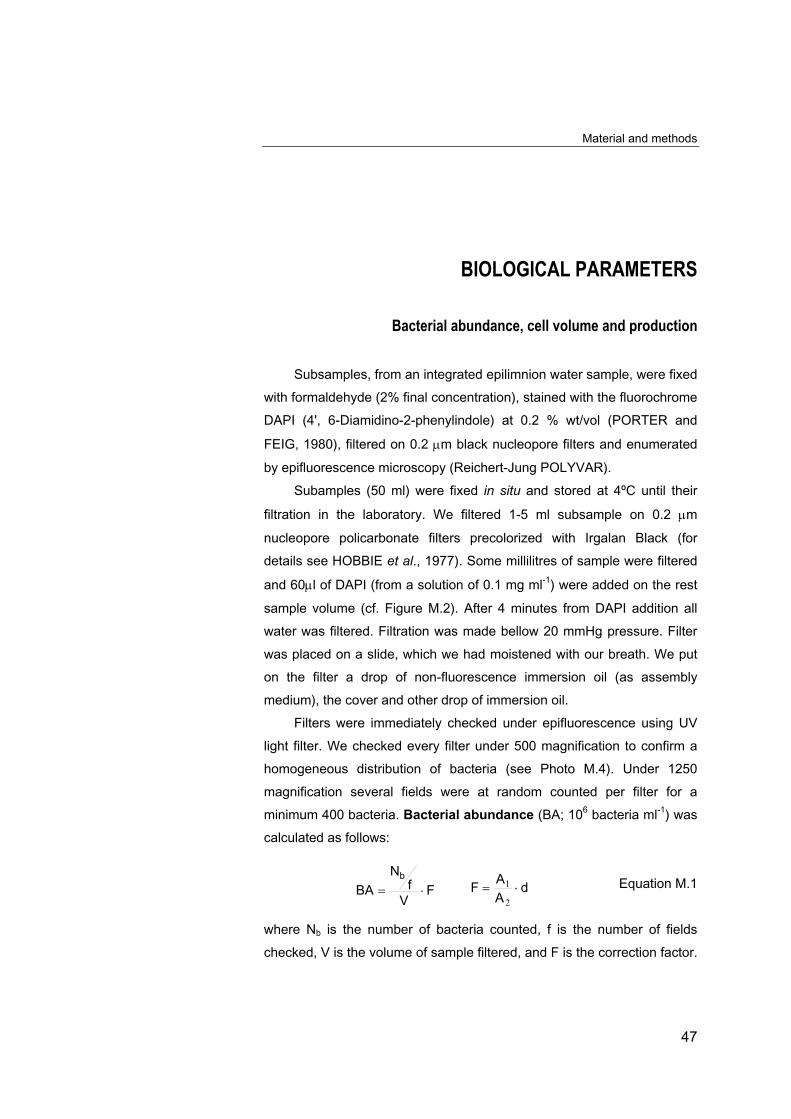
BIOLOGICAL PARAMETERS
Bacterial abundance, cell volume and production
Subsamples, from an integrated epilimnion water sample, were fixed
with formaldehyde (2% final concentration), stained with the fluorochrome
DAPI (4', 6-Diamidino-2-phenylindole) at 0.2 % wt/vol (PORTER and
FEIG, 1980), filtered on 0.2 µm black nucleopore filters and enumerated
by epifluorescence microscopy (Reichert-Jung POLYVAR).
Subamples (50 ml) were fixed in situ and stored at 4ºC until their
filtration in the laboratory. We filtered 1-5 ml subsample on 0.2 µm
nucleopore policarbonate filters precolorized with Irgalan Black (for
details see HOBBIE et al., 1977). Some millilitres of sample were filtered
and 60µl of DAPI (from a solution of 0.1 mg ml-1) were added on the rest
sample volume (cf. Figure M.2). After 4 minutes from DAPI addition all
water was filtered. Filtration was made bellow 20 mmHg pressure. Filter
was placed on a slide, which we had moistened with our breath. We put
on the filter a drop of non-fluorescence immersion oil (as assembly
medium), the cover and other drop of immersion oil.
Filters were immediately checked under epifluorescence using UV
light filter. We checked every filter under 500 magnification to confirm a
homogeneous distribution of bacteria (see Photo M.4). Under 1250
magnification several fields were at random counted per filter for a
minimum 400 bacteria. Bacterial abundance (BA; 106 bacteria ml-1) was
calculated as follows:
Equation M.1
where Nb is the number of bacteria counted, f is the number of fields
checked, V is the volume of sample filtered, and F is the correction factor.
FV
fN
BAb
⋅= dA
AF ⋅=
2
1
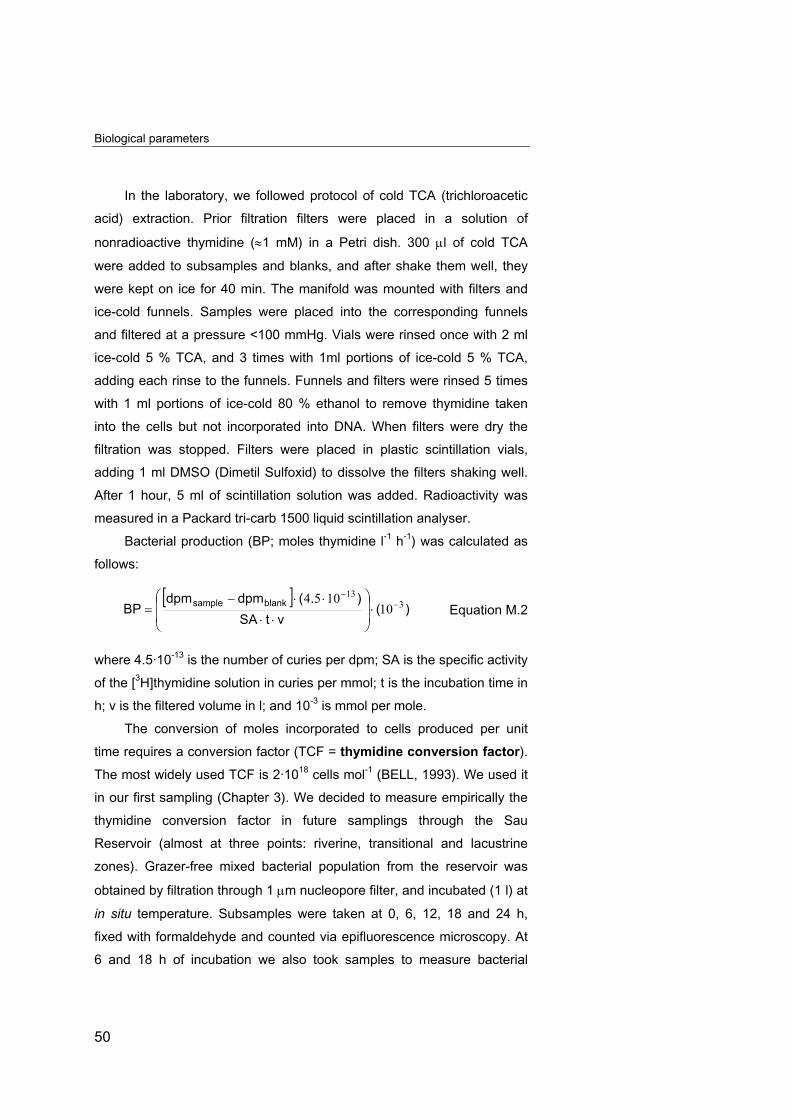
Biological parameters
4
A1 is the area of filtration on the filter, A2 is the area of one field checked
in microscope and d is the dilution of the sample by fixatives.
a
R
p
f
a
l
s
o
(
1
r
N
f
t
F
i
f
t
b
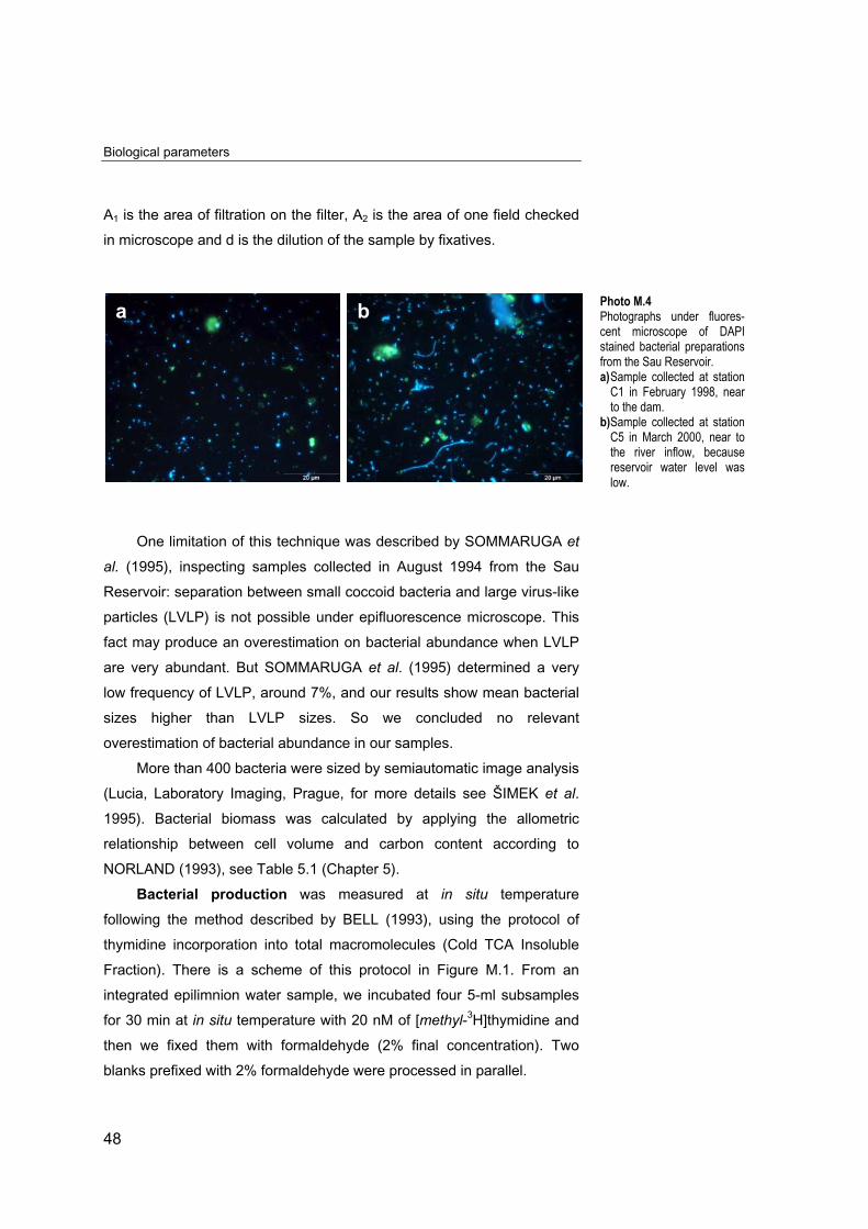
Photo M.4Photographs under fluores-
a8
One limitation of this technique w
l. (1995), inspecting samples collec
eservoir: separation between small c
articles (LVLP) is not possible unde
act may produce an overestimation o
re very abundant. But SOMMARUG
ow frequency of LVLP, around 7%, a
izes higher than LVLP sizes.
verestimation of bacterial abundance
More than 400 bacteria were size
Lucia, Laboratory Imaging, Prague,
995). Bacterial biomass was calcu
elationship between cell volume a
ORLAND (1993), see Table 5.1 (Cha
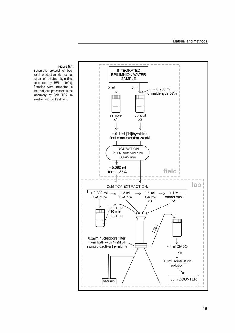
Bacterial production was m
ollowing the method described by B
hymidine incorporation into total ma
raction). There is a scheme of this
ntegrated epilimnion water sample, w
or 30 min at in situ temperature with
hen we fixed them with formaldehy
lanks prefixed with 2% formaldehyde
b
as described by SOMMARUGA et
ted in August 1994 from the Sau
occoid bacteria and large virus-like
r epifluorescence microscope. This
n bacterial abundance when LVLP
A et al. (1995) determined a very
nd our results show mean bacterial
So we concluded no relevant
in our samples.
d by semiautomatic image analysis
for more details see ŠIMEK et al.
lated by applying the allometric
nd carbon content according to
pter 5).
easured at in situ temperature
ELL (1993), using the protocol of
cromolecules (Cold TCA Insoluble
protocol in Figure M.1. From an
e incubated four 5-ml subsamples
20 nM of [methyl-3H]thymidine and
de (2% final concentration). Two
were processed in parallel.
cent microscope of DAPIstained bacterial preparationsfrom the Sau Reservoir.a) Sample collected at station
C1 in February 1998, nearto the dam.
b) Sample collected at stationC5 in March 2000, near tothe river inflow, becausereservoir water level waslow.
Material and methods
49
Figure M.1Schematic protocol of bac-terial production via icorpo-ration of tritiated thymidine,described by BELL (1993).Samples were incubated inthe field, and processed in thelaboratory by Cold TCA In-soluble Fraction treatment.
5 ml
INTEGRATEDEPILIMNION WATER
SAMPLE
+ 0.250 mlformaldehyde 37%
samplex4
+ 0.1 ml [ H]thymidinefinal concentration 20 nM
3
+ 0.250 mlformol 37%
+ 0.300 mlTCA 50%
+ 1 mlTCA 5%
x3
+ 2 mlTCA 5%
to stir up40 min
to stir up
+ 1 mletanol 80%
x5
vacuum
0.2 m nucleopore filterfrom bath with 1mM of
nonradioactive thymidine
µ
+ 5ml scintillationsolution
+ 1ml DMSO
Filt
er
dpm COUNTER
1h
5 ml
field
lab
Biological parameters
50
In the laboratory, we followed protocol of cold TCA (trichloroacetic
acid) extraction. Prior filtration filters were placed in a solution of
nonradioactive thymidine (≈1 mM) in a Petri dish. 300 µl of cold TCA
were added to subsamples and blanks, and after shake them well, they
were kept on ice for 40 min. The manifold was mounted with filters and
ice-cold funnels. Samples were placed into the corresponding funnels
and filtered at a pressure <100 mmHg. Vials were rinsed once with 2 ml
ice-cold 5 % TCA, and 3 times with 1ml portions of ice-cold 5 % TCA,
adding each rinse to the funnels. Funnels and filters were rinsed 5 times
with 1 ml portions of ice-cold 80 % ethanol to remove thymidine taken
into the cells but not incorporated into DNA. When filters were dry the
filtration was stopped. Filters were placed in plastic scintillation vials,
adding 1 ml DMSO (Dimetil Sulfoxid) to dissolve the filters shaking well.
After 1 hour, 5 ml of scintillation solution was added. Radioactivity was
measured in a Packard tri-carb 1500 liquid scintillation analyser.
Bacterial production (BP; moles thymidine l-1 h-1) was calculated as
follows:
Equation M.2
where 4.5·10-13 is the number of curies per dpm; SA is the specific activity
of the [3H]thymidine solution in curies per mmol; t is the incubation time in
h; v is the filtered volume in l; and 10-3 is mmol per mole.
The conversion of moles incorporated to cells produced per unit
time requires a conversion factor (TCF = thymidine conversion factor).
The most widely used TCF is 2·1018 cells mol-1 (BELL, 1993). We used it
in our first sampling (Chapter 3). We decided to measure empirically the
thymidine conversion factor in future samplings through the Sau
Reservoir (almost at three points: riverine, transitional and lacustrine
zones). Grazer-free mixed bacterial population from the reservoir was
obtained by filtration through 1 µm nucleopore filter, and incubated (1 l) at
in situ temperature. Subsamples were taken at 0, 6, 12, 18 and 24 h,
fixed with formaldehyde and counted via epifluorescence microscopy. At
6 and 18 h of incubation we also took samples to measure bacterial
[ ])(
vtSA
).(dpmdpmBP blanksample 3
13
101054 −
−
⋅
⋅⋅
⋅⋅−=
Material and methods
51
production via thymidine incorporation. The rate of bacterial growth (cells
l-1 h-1) from linear part of curve was divided by thymidine incorporation
(moles thymidine l-1 h-1) in the same period of time.
Protistan abundance, cell volume and grazing
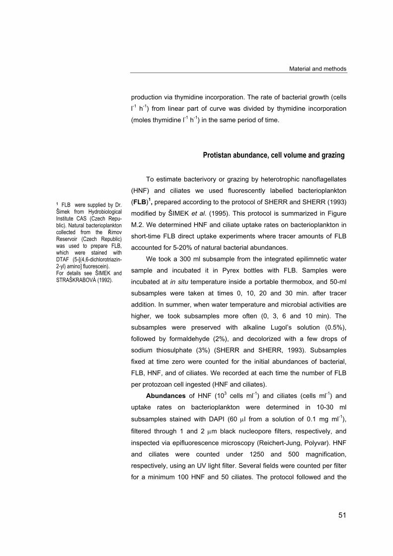
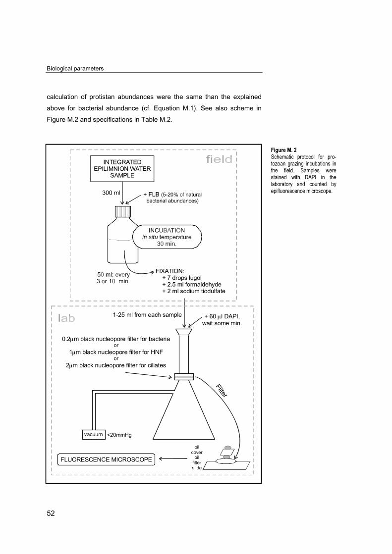
To estimate bacterivory or grazing by heterotrophic nanoflagellates
(HNF) and ciliates we used fluorescently labelled bacterioplankton
(FLB)1, prepared according to the protocol of SHERR and SHERR (1993)
modified by ŠIMEK et al. (1995). This protocol is summarized in Figure
M.2. We determined HNF and ciliate uptake rates on bacterioplankton in
short-time FLB direct uptake experiments where tracer amounts of FLB
accounted for 5-20% of natural bacterial abundances.
We took a 300 ml subsample from the integrated epilimnetic water
sample and incubated it in Pyrex bottles with FLB. Samples were
incubated at in situ temperature inside a portable thermobox, and 50-ml
subsamples were taken at times 0, 10, 20 and 30 min. after tracer
addition. In summer, when water temperature and microbial activities are
higher, we took subsamples more often (0, 3, 6 and 10 min). The
subsamples were preserved with alkaline Lugol’s solution (0.5%),
followed by formaldehyde (2%), and decolorized with a few drops of
sodium thiosulphate (3%) (SHERR and SHERR, 1993). Subsamples
fixed at time zero were counted for the initial abundances of bacterial,
FLB, HNF, and of ciliates. We recorded at each time the number of FLB
per protozoan cell ingested (HNF and ciliates).
Abundances of HNF (103 cells ml-1) and ciliates (cells ml-1) and
uptake rates on bacterioplankton were determined in 10-30 ml
subsamples stained with DAPI (60 µl from a solution of 0.1 mg ml-1),
filtered through 1 and 2 µm black nucleopore filters, respectively, and
inspected via epifluorescence microscopy (Reichert-Jung, Polyvar). HNF
and ciliates were counted under 1250 and 500 magnification,
respectively, using an UV light filter. Several fields were counted per filter
for a minimum 100 HNF and 50 ciliates. The protocol followed and the
1 FLB were supplied by Dr.Šimek from HydrobiologicalInstitute CAS (Czech Repu-blic). Natural bacterioplanktoncollected from the ŘimovReservoir (Czech Republic)was used to prepare FLB,which were stained withDTAF (5-[(4,6-dichlorotriazin-2-yl) amino] fluorescein).For details see ŠIMEK andSTRAŠKRABOVÁ (1992).
Biological parameters
52
calculation of protistan abundances were the same than the explained
above for bacterial abundance (cf. Equation M.1). See also scheme in
Figure M.2 and specifications in Table M.2.
Figure M. 2Schematic protocol for pro-tozoan grazing incubations inthe field. Samples werestained with DAPI in thelaboratory and counted byepifluorescence microscope.
INTEGRATEDEPILIMNION WATER
SAMPLE
300 ml + FLB (5-20% of naturalbacterial abundances)
FIXATION: + 7 drops lugol + 2.5 ml formaldehyde + 2 ml sodium tiodulfate
oil
coveroil
filterslide
<20mmHg
1-25 ml from each sample
0.2 m black nucleopore filter for bacteria
1 m black nucleopore filter for HNF
2 m black nucleopore filter for ciliates
µ
µ
µ
or
or
+ 60 l DAPI,wait some min.
µ
Filter
FLUORESCENCE MICROSCOPE
vacuum
Material and methods
53
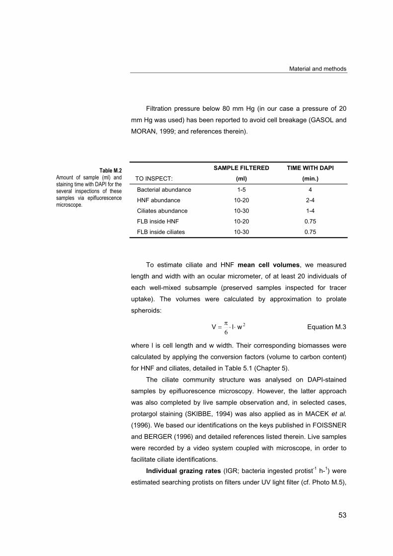
Filtration pressure below 80 mm Hg (in our case a pressure of 20
mm Hg was used) has been reported to avoid cell breakage (GASOL and
MORAN, 1999; and references therein).
SAMPLE FILTERED TIME WITH DAPI
TO INSPECT: (ml) (min.)
Bacterial abundance 1-5 4
HNF abundance 10-20 2-4
Ciliates abundance 10-30 1-4
FLB inside HNF 10-20 0.75
FLB inside ciliates 10-30 0.75
To estimate ciliate and HNF mean cell volumes, we measured
length and width with an ocular micrometer, of at least 20 individuals of
each well-mixed subsample (preserved samples inspected for tracer
uptake). The volumes were calculated by approximation to prolate
spheroids:
2
6wlV ⋅⋅
π= Equation M.3
where l is cell length and w width. Their corresponding biomasses were
calculated by applying the conversion factors (volume to carbon content)
for HNF and ciliates, detailed in Table 5.1 (Chapter 5).
The ciliate community structure was analysed on DAPI-stained
samples by epifluorescence microscopy. However, the latter approach
was also completed by live sample observation and, in selected cases,
protargol staining (SKIBBE, 1994) was also applied as in MACEK et al.
(1996). We based our identifications on the keys published in FOISSNER
and BERGER (1996) and detailed references listed therein. Live samples
were recorded by a video system coupled with microscope, in order to
facilitate ciliate identifications.
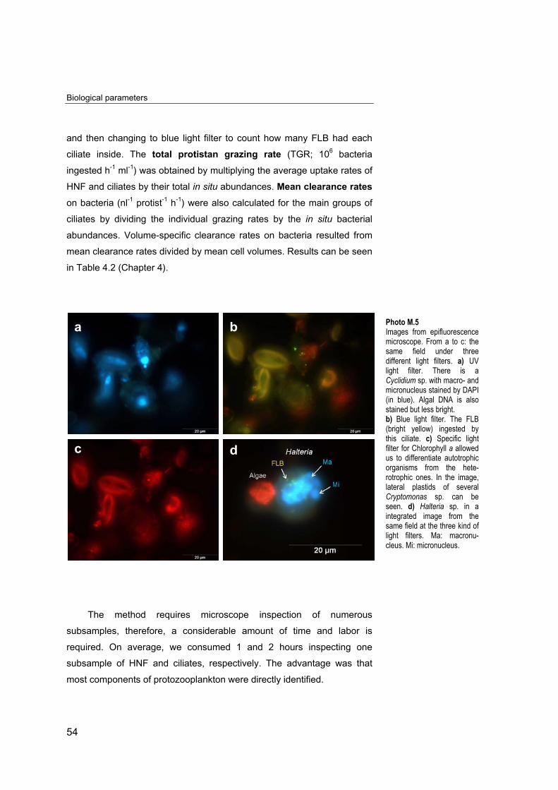
Individual grazing rates (IGR; bacteria ingested protist-1 h-1) were
estimated searching protists on filters under UV light filter (cf. Photo M.5),
Table M.2Amount of sample (ml) andstaining time with DAPI for theseveral inspections of thesesamples via epifluorescencemicroscope.
Biological parameters
5
and then changing to blue light filter to count how many FLB had each
ciliate inside. The total protistan grazing rate (TGR; 106 bacteria
ingested h-1 ml-1) was obtained by multiplying the average uptake rates of
HNF and ciliates by their total in situ abundances. Mean clearance rates
on bacteria (nl-1 protist-1 h-1) were also calculated for the main groups of
ciliates by dividing the individual grazing rates by the in situ bacterial
abundances. Volume-specific clearance rates on bacteria resulted from
mean clearance rates divided by mean cell volumes. Results can be seen
in Table 4.2 (Chapter 4).
s
r
s
m
Photo M.5Images from epifluorescence
a4
The method requires micro
ubsamples, therefore, a considera
equired. On average, we consume
ubsample of HNF and ciliates, resp
ost components of protozooplankton
b
microscope. From a to c: thesame field under threedifferent light filters. a) UVlight filter. There is aCyclidium sp. with macro- andmicronucleus stained by DAPI(in blue). Algal DNA is alsostained but less bright.b) Blue light filter. The FLB(bright yellow) ingested bythis ciliate. c) Specific lightfilter for Chlorophyll a allowed c dscope inspection of numerous
ble amount of time and labor is
d 1 and 2 hours inspecting one
ectively. The advantage was that
were directly identified.
us to differentiate autotrophicorganisms from the hete-rotrophic ones. In the image,lateral plastids of severalCryptomonas sp. can beseen. d) Halteria sp. in aintegrated image from thesame field at the three kind oflight filters. Ma: macronu-cleus. Mi: micronucleus.
Material and methods
55
Chlorophyll a
The chlorophyll a content in phytoplankton collected on Whatman
GF/F glass microfibre filters was analysed by using the trichromatic
method of JEFFREY and HUMPHREY (1975).
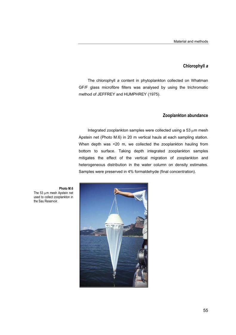
Zooplankton abundance
Integrated zooplankton samples were collected using a 53 µm mesh
Apstein net (Photo M.6) in 20 m vertical hauls at each sampling station.
When depth was <20 m, we collected the zooplankton hauling from
bottom to surface. Taking depth integrated zooplankton samples
mitigates the effect of the vertical migration of zooplankton and
heterogeneous distribution in the water column on density estimates.
Samples were preserved in 4% formaldehyde (final concentration).
Photo M.6The 53 µm mesh Apstein netused to collect zooplankton inthe Sau Reservoir.
Biological parameters
56
We also obtained a live replicate sample for direct observation in
order to identify rotifer species. The fixed samples were immediately
sieved in the laboratory. Six mesh sizes (53, 100, 150, 250, 500 and 710
µm) were used to define the size distribution of the sample. Each
subsample was sedimented in a sedimentation chamber and quantified in
an inverted microscope (OLYMPUS T041) by counting at least 60
individuals from the main species (McCAULEY, 1984).
The zooplankton biomass in the epilimnion was calculated as the
proportional biomass of the total in the haul present in the epilimnion. Dry
weights (DW) were estimated by geometric approximations in RUTTNER-
KOLISKO (1977) for rotifers, considering an approximate density of ρ = 1
g cm-3 and that DW was about 10 % of fresh weight (LATJA and
SALONEN, 1978) except for Asplachna (4 %; DUMONT et al., 1975).
Mean weights for crustacean species were estimated from regression
equations in BOTTRELL et al. (1976) and McCAULEY (1984). The
biomass of eggs was not considered.