Embed Size (px)
Citation preview
Processor Sharing Queueing Models of Mixed Scheduling Disciplines for Time Shared Systems
L. KLEINROCK AND R. R. MUNTZ
University of California, Los Angeles, California
ABSTRACT. Scheduling algorithms for time shared computing facilities are considered in terms of a queueing theory model. The extremely useful limit of "processor sharing" is adopted, wherein the quantum of service shrinks to zero; this approach greatly simplifies the problem. A class of algorithms is studied for which the scheduling discipline may change for a given job as a function of the amount of service received by that job. These multilevel disciplines form a natural extension to many of the disciplines previously considered.
The average response time for jobs conditioned on their service requirement is solved for. Explicit solutions are given for the system M/G/1 in which levels may be first come first served (FCFS), feedback (FB), or round-robin (RR) in any order. The service time distribution is restricted to be a polynomial times an exponential for the case of RR.
Examples are described for which the average response time is plotted. These examples display the great versatili ty of the results and demonstrate the flexibility available for the intelligent design of discriminatory treatment among jobs (in favor of short jobs and against long iobs) in time shared computer systems.
KEY WORDS AND PHRASES : time sharing, operating systems, queues, mathematical models
CR C A T E G O R I E S : 3.89, 4.39, 5.5
1. Introduction
Queueing models have been used successful ly in the analys is of t ime shared com- p u t e r sys t ems since the ap pe a ra nc e of t he first appl ied p a p e r in th is field in 1964 [1]. A recent su rvey of th is work is given b y M c K i n n e y [2]. One of the first pape r s to consider the effect of feedback in queueing sys tems was due to Tak£cs [3].
One of t he goals in a t ime shared c o m p u t e r sys t em is to p rov ide r ap id response to those t a sks which are i n t e r ac t ive and which p lace f requen t , bu t small , d e m a n d s on the sys tem. As a resul t , the sys tem schedul ing a lgo r i t hm mus t iden t i fy those d e m a n d s which are small , and p rov ide t h e m wi th p re fe ren t i a l t r e a t m e n t over l a rge r demands . Since we assume t h a t t he scheduler has no explici t knowledge of job process ing t imes, th is ident i f ica t ion is accompl i shed impl ic i t ly b y " t e s t i n g " jobs. T h a t is, jobs are r ap id ly p rov ided smal l a moun t s of process ing and, if t h e y are short , t h e y will d e p a r t r a the r qu ick ly ; otherwise, t h e y will l inger while other , newer jobs are p rov ided this r ap id service, etc., t hus p rov id ing good response to smal l demands .
Copyright © 1972, Association for Computing Machinery, Inc. General permission to republish, but not for profit, all or part of this material is granted, provided that reference is made to this publication, to its date of issue, and to the fact that reprinting privileges were granted by permission of the Association for Computing Machinery. Authors' address: University of California, Computer Science Department, School of Engineer- ing and Applied Science, Los Angeles, CA 90024. This work was supported by the Advanced Research Projects Agency of the Department of Defense (DAHC-15-69-C-0285).
Journal of the Association for Computing Machinery, Vol. 19, No. 3, July 1972, pp. 464-482.
Processor Sharing Queueing Models 465
Generally, an arrival enters the time shared system and competes for the atten- tion of a single processing unit. This arrival is forced to wait in a system of queues until he is permitted a quantum of service time; when this quantum expires, he is then required to join the system of queues to await his second quantum, etc. The precise model for the system is developed in Section 2. In 1967 the notion of allow- ing the quantum to shrink to zero was studied [4] and was referred to as "processor sharing"; in 1966 Schrage [18] also studied the zero-quantum limit. As the name implies, this zero-quantum limit provides a share or portion of the processing unit to many customers simultaneously; in the case of round-robin (RR) scheduling [4], all customers in the system simultaneously share (equally or on a priority basis) the processor, whereas in the feedback (FB) scheduling [5] only that set of customers with the smallest attained service share the processor. We use the term processor sharing here since it is the processing unit itself (the central processing unit of the computer) which is being shared among the set of the customers; the phrase "time sharing" is reserved to imply that customers are waiting sequentially for their turn to use the entire processor for a finite quantum. In studying the literature one finds that the obtained results appear in a rather complex form and this complexity arises from the fact that the quantum is typically assumed to be finite as opposed to infinitesimal. When one allows the quantmn to shrink to zero, giving rise to a processor sharing system, then the difficulty in analysis as well as in the form of results disappears in large part; one is thus encouraged to consider the processor sharing case. Clearly, this limit of infinitestimal quantum 1 is an ideal and can seldom be reached in practice due to overhead considerations; nevertheless, its extreme simplicity in analysis and results brings us to the studies reported in this paper.
The two processor sharing systems studied in the past are the RR and the FB [4, 5]. Typically, the quantity solved for is T(t), the expected response time con- ditioned on the customer's service time t; response time is the elapsed time from when a customer enters the system until he leaves completely serviced. This measure is especially important since it exposes the preferential treatment given to short jobs at the expense of the long jobs. Clearly, this discrimination is purposeful since, as stated above, it is the desire in time shared systems that small requests should be allowed to pass through the system quickly. In 1969 the distribution for the response time in the RR system was found [6]. In this paper we consider the case of mixed scheduling algorithms whereby customers are treated according to the RR algo- rithms, the FB algorithm, or first come first served (FCFS) algorithm, depending upon how much total service time they h~ve already received. Thus, as a customer proceeds through the system obtaining service at various rates, he is treated accord- ing to different disciplines; the policy which is applied among customers in different levels is that of the FB system as explained further in Section 2. Thus, natural generalization of the previously studied processor sharing systems allows us to create a large number of new and interesting disciplines whose solutions we present.
A more restricted study of this sort was reported by the authors in [16]. Here we make use of the additional results from [11] to generalize our analysis.
~This l i m i t i ng case is no t un l ike t h e d i f fus ion a p p r o x i m a t i o n for q u e u e s (see, for e x a m p l e ,
Gaver [17]).
Journal of the Association for Computing Machinery, Vol. 19, No. 3, .July 1972
466 L. KLEINROCK AND R. R. MUNTZ
2. The Model
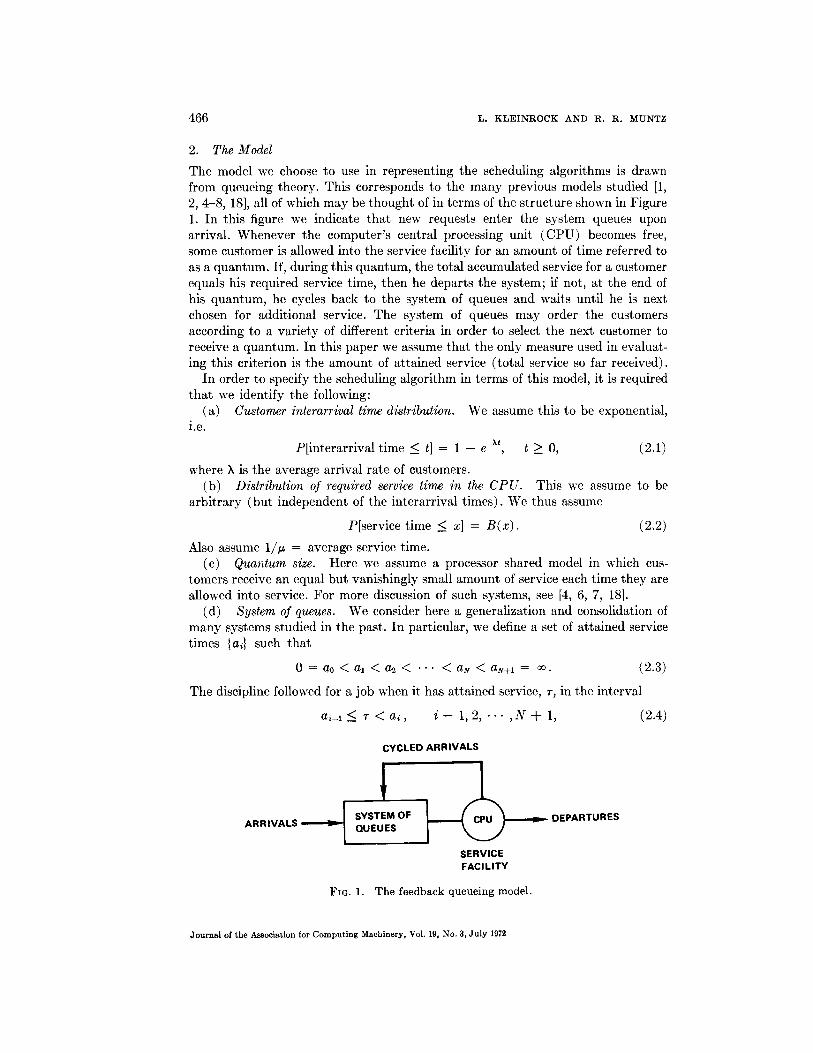
The model we choose to use in representing the scheduling algorithms is drawn from queueing theory. This corresponds to the many previous models studied [1, 2, 4-8, 18], all of which may be thought of in terms of the structure shown in Figure 1. In this figure we indicate tha t new requests enter the system queues upon arrival. Whenever the computer ' s central processing unit (CPU) becomes free, some customer is allowed into the service facility for an amount of t ime referred to as a quantum. If, during this quantum, the total accumulated service for a customer equals his required service time, then he departs the system; if not, at the end of his quantum, he cycles back to the system of queues and waits until he is next chosen for additional service. The system of queues may order the customers according to a variety of different criteria in order to select the next customer to receive a quantum. In this paper we assume tha t the only measure used in evaluat- ing this criterion is the amount of attained service (total service so far received).
In order to specify the scheduling algorithm in terms of this model, it is required tha t we identify the following:
(a) Customer interarrival time distribution. We assume this to be exponential, i.e.
P[interarrival t ime _~ t] = 1 - e TM, t _> 0, (2.1)
where ~ is the average arrival rate of customers. (b) Distribution of required service time in the CPU. This we assume to be
arbi t rary (but independent of the interarrival t imes). We thus assume
P[service t ime ~ x] = B(x) . (2.2)
Also assume 1/~ = average service time. (c) Quantum size. Here we assume a processor shared model in which cus-
tomers receive an equal but vanishingly small amount of service each t ime they are allowed into service. For more discussion of such systems, see [4, 6, 7, 18].
(d) System of queues. We consider here a generalization and consolidation of many systems studied in the past. In particular, we define a set of at tained service times {ai} such tha t
0 = a0 < a l ~ a 2 ~ . . . < a N ~aN+l = oo. (2.3)
The discipline followed for ~ job when it has attained service, r, in the interval
a~-I ~ r < a i , i - 1, 2, . . . , N ~ 1, (2.4)
. • SYSTEM OF ARRIVALS QUEUES
CYCLED ARRIVALS
SERVICE FACILITY
~- DEPARTURES
FIG. 1. T h e f e e d b a c k q u e u e i n g mode l .
Journal of the Association for Computing Machinery, Vol. 19, No. 3, July 1972
Processor Sharing Queueing Models 467
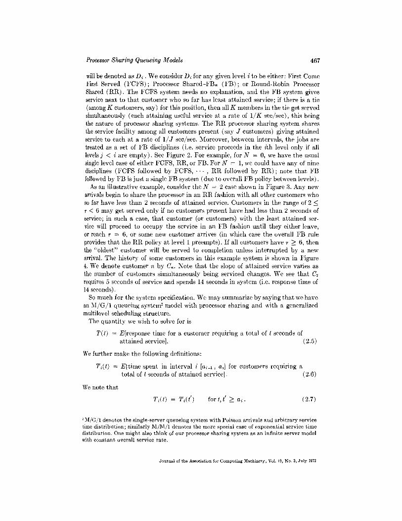
will be denoted as Di • We consider D~ for any given level i to be either: First Come First Served (FCFS) ; Processor Shared-FB, (FB) ; or Round-Robin Processor Shared (RR) . The FCFS system needs no explanation, and the FB system gives service next to that customer who so far has least attained service; if there is a tie (among K customers, say) for this position, then all K members in the tie get served simultaneously (each attaining useful service at a rate of 1/K see/see), this being the nature of processor sharing systems. The RR processor sharing system shares the service facility among all customers present (say J customers) giving attained service to each at a rate of 1/J see/see. Moreover, between intervals, the jobs are treated as a set of FB disciplines (i.e. service proceeds in the ith level only if all levels j < i are empty) . See Figure 2. For example, for N = 0, we have the usual single level case of either FCFS, RR, or FB. For N = 1, we could have any of nine disciplines (FCFS followed by FCFS, . . . , RR followed by RR) ; note tha t FB followed by FB is just a single FB system (due to overall FB policy between levels).
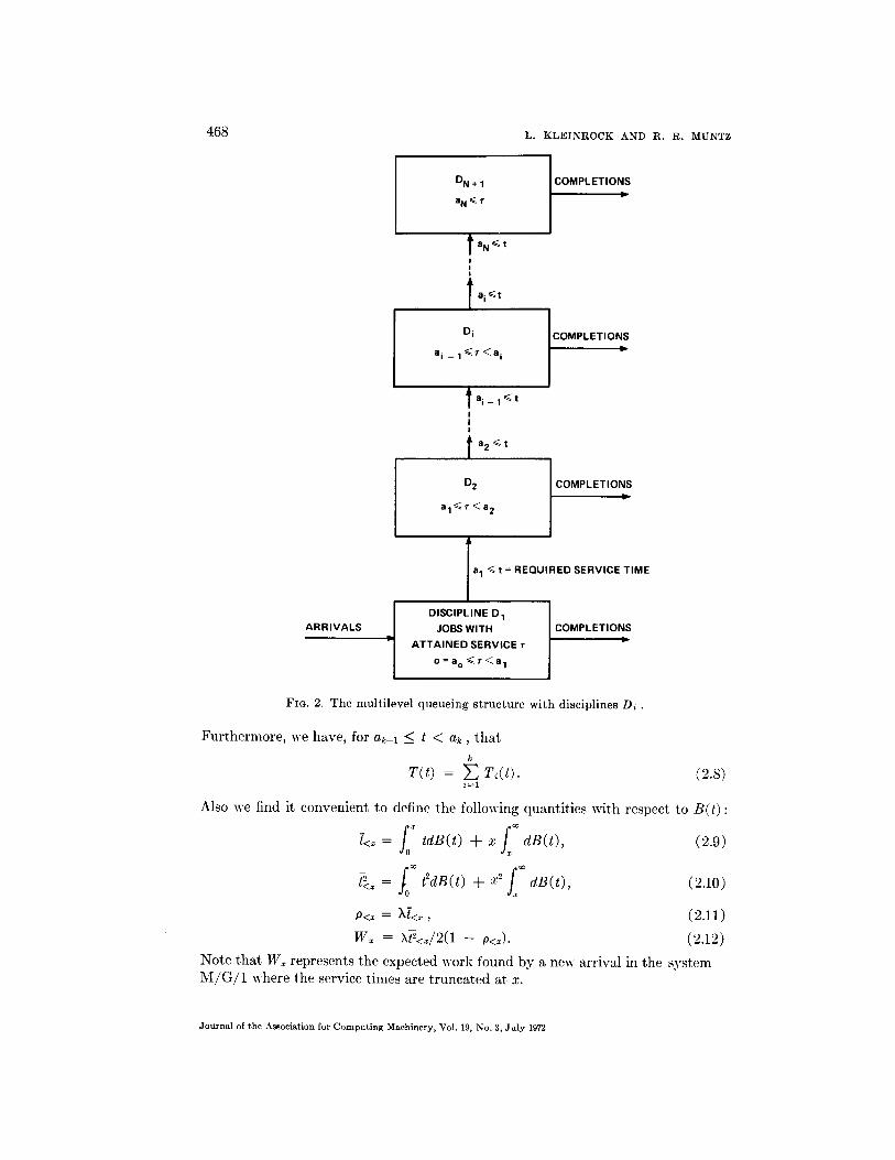
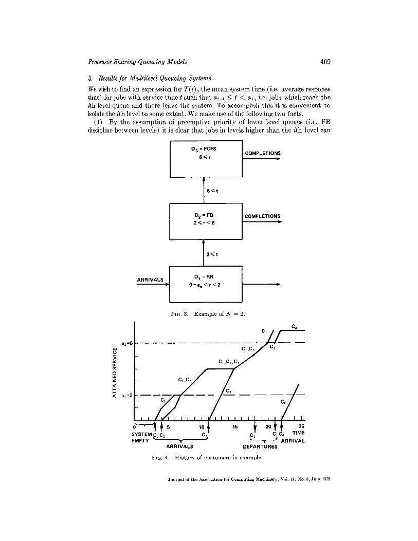
As an illustrative example, consider the N = 2 case shown in Figure 3. Any new arrivals begin to share the processor in an RR fashion with all other customers who so far have less than 2 seconds of attained service. Customers in the range of 2 _~ r < 6 may get served only if no customers present have had less than 2 seconds of service; in such a case, that customer (or customers) with the least attained ser- vice will proceed to occupy the service in an FB fashion until they either leave, or reach r = 6, or some new customer arrives (in which case the overall FB rule provides that the RR policy at level 1 preempts). If all customers have r > 6, then the "oldest" customer will be served to completion unless interrupted by a new arrival. The history of some customers in this example system is shown in Figure 4. We denote customer n by Cn. Note that the slope of attained service varies as the number of customers simultaneously being serviced changes. We see that C~ requires 5 seconds of service and spends 14 seconds in system (i.e, response time of 14 seconds).
So much for the system specification. We may summarize by saying that we have an M/G/1 queueing system 2 model with processor sharing and with a generalized multilevel scheduling structure.
The quanti ty we wish to solve for is
T(t) = E[response time for a customer requiring a total of t seconds of attained service}. (2.5)
We further make the following definitions:
T~(t) = E{time spent in interval i [aT-l, a~] for customers requiring a total of t seconds of attained service}. (2.6)
We note that.
T~(t) = T~(t') for t,t ' ~_ a~. (2.7)
M/G/1 denotes the single-server queueing system with Poisson arrivals and arbi t rary service time distr ibution; similarly M/M/1 denotes the more special case of exponential service time distribution. One might also think of our processor sharing system as an infinite server model with constant overall service rate.
Journal of the Association for Computing Machinery, Vol. 19, No. 3, July 1972
468 L. KLEINROCK AND R. R. MUNTZ
DN+I
aN<r
t aN~<t !
l a i ~<t
Di
a i _ l ~ v < a i
COMPLETIONS
COMPLETIONS
• a i _ l ~ t i I i l a 2 ~ t
D 2
al~<r<a 2
COMPLETIONS v
ARRIVALS
a I <~ t = REQUIRED SERVICE TIME
t DISCIPLINE D 1 JOBS WITH
ATTAINED SERVICE r O = a o ~ r < a 1
COMPLETIONS
FiG. 2. The multilevel queueing structure with disciplines Di.
Furthermore, we have, for ak_l < t < ak, that
k
T( t ) = ~ T d t ) . (2.8) i = l
Also we find it convenient to define the following quantities with respect to B( t ) :
f0 ~ ff t<x = tdB( t ) + x d B ( t ) , x
t ~ = t~dB(t) + x ~ d B ( t ) , x
p<: = X~<~,
W~ = ~/i<~/2(1 -- p<~).
Note that Wz represents the expected work found by a new arrival in the system M / G / 1 where the service times are truncated at x.
(2.9)
(2.10)
(2.11) (2.12)
Journal of the Association for Computing Machinery, Vol. 19, No. 3, July 1972
Processor Sharing Queueing Models 469
3. Results for Multilevel Queueing Systems
We wish to find an expression for T(t) , the mean system time (i.e. average response time) for jobs with service time t such that ai-i _~ t ~ ai, i.e. jobs which reach the ith level queue and there leave the system. To accomplish this it is convenient to isolate the ith level to some extent. We make use of the following two facts.
(1) By the assumption of preemptive priority of lower level queues (i.e. FB discipline between levels) it is clear that jobs in levels higher than the ith level can
D 3 = F C F S
6~7 COMPLETIONS
1 6 ~ t
D 2 = FB
2~<r<6 COMPLETIONS
uJ (J > CC uJ o0 ¢3 uJ Z
k- k-
a2 =6
a t =2
ARRIVALS
T 2~<t
_ I D1 = R R
r I 0=a°~<T<2
FIG. 3. Example of N = 2.
I I
o'--,-li SYSTEM .C. C, EMPTY ~' "
ARRIVALS
C3
Ci o C t / C3
C I , C y
c,,J /
_ _ - - C j . - - C ~ / '
I I i i / I I 10~ 15 ~ 2 0 t J ~ 25
C~. C: Ca C, TIME J x J ARRIVAL
DEPARTURES
FIG. 4. History of customers in example.
Journal of the Association for Computing Machinery, Vol. 19, No. 3, July 1972
470 L. K L E I N R O C K AND R. R. MUNTZ
be ignored. This follows since these jobs cannot interfere with the servicing of the lower levels.
(2) We are interested in jobs that will reach the ith level queue and then depart from the system before passing to the (i + 1) -th level. The system time of such a job can be thought of as occurring in two parts. The first portion is the time from the job's arrival to the queueing system until the group at the ith level is serviced for the first time after this job has reached the ith level. The second portion starts with the end of the first portion and ends when the job leaves the system. It is easy to see that both the first and second portions of the job's system time are unaffected by the service disciplines used in levels 1 through i - 1. Therefore we "can assume any convenient disciplines. In fact, all these levels can be lumped into one equivalent level which services jobs with attained service between 0 and ai_l seconds using any service discipline.
From (1) and (2) above it follows that we can solve for T ( t ) for jobs that leave the system from the ith level by considering a two level system. The lower level services jobs with attained service between 0 and aN-j, whereas the second level services jobs with attained service between ai-~ and a~. Jobs that would have passed to the (i + 1)-th level after receiving a~ seconds of service in the originalsystem are now assumed to leave the system at that point. In other words the service times are truncated at a~.
3.1 iTH LEVEL DISCIPLINE IS FB. Consider the two level system with the sec- ond level corresponding to the i th level of the original system. Since we are free to choose this discipline used in the lower level, we can assume that the FB discipline is used in this level as well. Clearly the two level system behaves like a single level FB system with service times t runcated at a~. The solution for such a system is known [5, 9]:
T ( t ) = t / ( 1 -- p<t) + IT<t/J2(1 -- p<t)2]. (3.1)
3.2 iwn LEVEL DISCIPLINE IS FCFS. Consider again the two level system with breakpoints at a~_~ and a~. Regardless of the discipline in the lower level, a tagged job entering the system will be delayed by the sum of (a) the work currently in both levels ( = Wo~) plus (b) any new arrivals to the lower level queue during the interval [average T(t)] this job is in the system. These new arrivals form a Poisson process with parameter ~ and their contribution to the delay is a random variable whose first and second moments are t<a~--i and ~<,~_~ respectively.
Thus we have
and so
T ( t ) = W~, + kta,_l T ( t ) + t
T ( t ) = (Wa, + t ) / (1 - p<~,_,), (3.2)
where Wa~ is given by eq. (2.12). It is also possible to use these methods for solving last come first served and random order of service at any level.
3.3 iT~ LEVEL DISCIPLINE IS RR. In this case, our results are limited in the ith interval to service distributions in which
B ( x ) = 1 - p ( x ) e -~x, ai-1 < x < a i , (3.3)
p ( x ) = po "-t- p l x + . " + pax ~. (3.4)
Journal of the Association for Computing Machinery, Vol. 19, No. 3, July 1972
Processor Sharing Queueing Models 471
The service time distribution F ( x ) for this ith interval is then
~B(ai-1 + x ) -- B(a i -1 ) • f ( z ) ] - 1 -- B ( ~ _ ~ = 1 -- q ( x )e -ax 0 < x < ai - ai-1
= ( 3 . 3 ' )
I1 x > al -- ai-1,
where
q(x ) = e-~ai- lp(ai-1 + x) 1 - B(a~-~) = qo -~ qlx + . . . + q~x '~. (3 .4 ' )
Thus we permit in this interval service time distributions of the form: 1 minus a polynomial of degree n times an exponential. The analysis of this system appears in Ill]; we make use of these results below. Nevertheless, we develop our analysis as far as possible for the case of general B ( x ) before specializing to the class given by eqs. (3.3) and (3.4).
We start by considering the two level system with breakpoints at a~_l and a~. Consider the busy periods of the lower level. During each such busy period there may be a number of jobs that pass to the higher level. We choose to consider these arrivals to the higher level as occurring at the end of the lower level busy period so that there is a bulk arrival to the higher level at this time. We also choose to tem- porarily delete these lower level busy periods from the time axis. In effect we create a virtual time axis telescoped to delete the lower level busy periods. Since the time from the end of one lower level busy period to the start of the next is exponentially distributed (Poisson arrivals!), the arrivals to the higher level appear in virtual time to be bulk arrivals at instants generated from a Poisson process with parameter ~,.
Consider a tagged job that required t = a~-i + r seconds of service (0 < r _< a~ - a~_l). Let a~ be the mean real time the job spends in the system until its arrival (at the end of the lower level busy period) at the higher level queue. Let a2(r) be the mean virtual time the job spends in the higher level queue, al can be calculated as follows. The initial delay is equal to the mean work the job finds in the lower level on arrival plus the a~_~ seconds of work that it contributed to the lower level. Therefore
Cgl = Wai_ 1 -~- ~tai_lOll + ai-1 and so
al = [1/(1 - p<a~_l)]{Wa~_, + a~-l}. (3.5)
If a2(T) is the mean virtual time the job spends in the higher level, we can easily convert this to the mean real time spent in this level. In the virtual time interval a2(T) there are an average of ha2(T) lower level busy periods that have been ignored. Each of these has a mean length of t<a~_l/(1 -- P<a~-l)- Therefore, the mean real time the job spends in the higher level is given by
a2(T) -Jr Xa2(r)" t<ai_ , / (1 -- P<a,_,) = a 2 ( T ) / ( 1 -- P<a,_,). (3.6)
Combining these results we see that a job requiring t = a~_l + r seconds of service has mean system time given by
T(a~_l + 7) = [1/(1 - - P<ai_l)]{Wai_l -~- ai-1 -~ O/2(T)}. (3.7)
Journal of the Association for Computing Machinery, Voll 19, No. 3, July 1972
472 L. K L E I N R O C K A N D R. R . M U N T Z
The only unknown quanti ty in this equation is a2(r) . To solve for a2(r) we must, in general, consider an M / G / 1 system with bulk arrival and RR processor sharing. The only exception is the case of RR at the first level which has only single arrivals. Since the higher level queues can be ignored, the solution in this exceptional case is the same as for a round-robin single level system with service times truncated at al • Therefore, from [8] we have for the first level,
T( t ) = t / (1 -- P<a,) 0 __~ t < a~. (3.8)
Let us now consider the bulk arrival R R system in isolation in order to solve for the virtual time spent in the higher level queue a2(v). The service time distribution for this bulk arrival system is
~[B(ai_i -Jr x) - B(a~_l)]/[1 -- B(ai_i)], 0 < x < al -- at_l , F ( x )
(1, x ~ a i - a t - 1 .
Note that the utilization factor for this bulk system is
p = Xd /u l , (3.9)
where d is the mean number of arrivals in a bulk and 1/u~ is the mean of the distribu- tion F ( x ) . Let us begin by solving for 5. This we do for the general case a~-i, a~. d is just the mean number of jobs that arrive during a low level busy period and require more than at-1 seconds of service. Therefore d must satisfy the equation
5 = XT<~,_,a + [1 -- B(a~_l)]l. (3.10)
In this equation Xt<~_ 1 is the mean number of jobs that arrive during the service time of the first job in the busy period. Since each of these jobs in effect generates a busy period, there are an average of ht<,~_fl arrivals to the upper level queue due to these jobs. The second term is just the average number of times that the first job in the busy period will require more than a~-i seconds of service. Clearly then
d = [1 -- B(a~_l)]/[1 -- P<~-i]- (3.11)
In [11], an integral equation is derived which defines a2 (T) for the RR bulk arrival system; we repeat tha t equation below:
' f0 ' a2 ( r ) = Xd a2(x)[1 -- F ( x + r ) ] d x
P
+ X5 J, c~2'(x)[1 -- F ( r - - X)] d x
-1- 1 + b[1 -- F ( r ) ] , (3.12)
where a2' (r ) = do~2( r) /dr , and b is the mean number of arrivals with the tagged j ob. The solution to this integral equation for the restricted service time distributions as given in eqs. (3.3') and (3.4') is also given in [11], and for our problem takes the form
~(,) -
1 -- Xa ~
b ~2,1 ( ~ - - 7m2) '}+1
Q0(~m)[1 - e -~m~] - Ul~Tm)'~ ~- ~e -~mxl~te~m~ -- 1] [Q0(~m) + e-~mXlQl(~m)]%,
, ( 3 .13 )
Journal of the Association for Comuutin~ Machinery. Vol. 19. No. 3 . . h d v 1972
Processor Sharing Queueing Models 473
where
xl = a i - a / _ 1 , ( 3 . 1 4 )
Qo(x) = (x + f~)~+l - X~ ~ q(k)(0)(x + ~)~-k, (3.15) k~0
Ql(x) = X5 ~ e-~X~q(k)(xl)(x + X) ~-k, (3.16)
Q2(x) = Qo(x)Qo(-x) - Ql(x)Q~(-x), (3.17)
and where eq. (3.17) has roots (occurring in pairs) x = -%~, , ~m for m = 1, 2, • • • , n + 1 and the notat ion f(k)(,y) denotes the kth derivative of f with respect to its argument evaluated at a value ~.
in the solution for c~2(T) given in eq. (3.13), we are required to compute b (mean number of arrivals with a tagged job). This we do by first deriving an expression for
G(z) = ~ P[bulk size = k]z k (3.18) k=0
which is the probabil i ty generating function (z-transform) for the bulk size. Either by direct arguments based upon busy periods or by use of the method of collective marks [12], we readily arrive at
G(z) = [1 -- B(ai-1)]z ~ (~kai-1)J e -Xa i - l [G(z ) ] J j=0 3!
[fo'i-lj~o (Xt)Je-Xt[G(z)] j dB(t) + B(a i - i ) - ~ - B ~ ) _ J " (3.19)
In eq. (3.19) the first t e rm is conditioned on the assumption tha t the customer who preempts service from those at level i reaches the ith level; the second te rm assumes that he does not reach level i. Equat ion (3.19) reduces to
G ( z ) LI ~r~ ~ l ~ - ~ a ~ _ l [ 1 - ~ ( z ) J fo a~-~ . . . . \ ~ i - I / l ~ + e -xt[1-G(z)] dB(t) . (3.20)
For arbi trary B(x), we c~Imot reduce this last expression any further. Nevertheless, we can obtain moments from it. In particular, from the definition of d, we obtain
-: Z / ( z ) Iz=i = [1 - B(a~_~) ] / [1 - X~<o,_~],
which is exactly as o~,~ ained by more direct arguments in eq. (3.11). However, we are seeking b. For this we must calculate
G"(z) [~=1 = [(d)2/(1 -- p<~_l)][2Xa~_~(1 -- p<~,_~) + X2~<~,_~]. (3.21)
Now since the mean group size ( 1 + b) of a tagged customer's group is related to the bulk size distribution as the mean spread is related to the inter-event distribution (namely, the mean spread equals the second moment of the inter-event interval divided by the first moment) [13], we have
1 + b = (second moment of bulk size)/(f irs t moment of bulk size) (3.22) or
e r r ( z ) z ~ i " b - G'(z) (3.23)
Journal of the Association for Computing Machinery, Vol. 19, No. 3, July 1972
474 L. K L E I N R O C K AND R. R. MUNTZ
From eq. (3.20) we get
27i b = [d/(1 - p<~,_~)][2ka~_~(1 - P<a~_x) + k t <~_~]. (3.24)
Having solved for a2(r) we may now substitute back into eq. (3.7) which solves the case when the ith level discipline is R R and service t ime is of the form given in eqs. (3.3') and (3.4'). [Note tha t for i = 1, the solution given in eq. (3.8) is good for any B ( x ) . ]
I t is instructive to display the solution for T ( t ) explicitly in a special case for our ith level R R discipline. We choose the multilevel system with M / M / 1 and solve for T(a~_~ + r) after substituting a2(r) into eq. (3.7). Note for M / M / 1 tha t q(t ) = q0 = 1. Also, from eqs. (3.14)-(3.17), and choosing ~ = #,
Qo(x) = x + ~ - kd, (3.25)
Q~(x) = h~e -~1, (3.26)
Q~(x) = #~ - 2#~d + (~d)2(1 - e -2~x~) - x2; (3.27)
thus the roots of Q~(x) are
± ~t = ± [ 2 _ 2~kd + (~5)2(1 -- e-2~x~)] i, (3.28)
/.~i = / u - l ( 1 ; ( 3 . 2 9 )
thus from these and eq. (3.13), we get
~(~) -
1 - - kd#T ~
+ b(# 2 -- 7~2)[(71 + # - kS)(1 - e - ~ ' ) -- Xde-(Z+vt)~l(e ~ -- 1)] (3.30) 2~d'y12['y1 + # - - hd(1 -- e-(,+~l)~,)]
Also from eqs. (2.9) and (2.10) we obtain
t<~ = # - 1 ( 1 - - e - " X ) , ( 3 . 3 1 )
~<~ = 2~-2(1 -- e - ~ -- #xe-~X). (3.32)
We may substitute these last two equations into eqs. (3.11) and (3.24) to obtain a and b explicitly. Also, we note from eqs. (2.12) and (3.32) tha t
Wa,_~ = [k(1 - e - ~ ' - ~ - ~a~_le - '~ - ' ) ] /~2[1 - (~ /# ) (1 - e - ~ - ~ ) ] . (3.33)
Finally, we may substitute this expression for W,~_~ and eq. (3.30) which gives (~2(r) into eq. (3.7) which gives us the explicit form for T ( r ) .
4. E x a m p l e s
In this section we demonstrate through examples the nature of the results we have obtained. Recall tha t we have given explicit solutions for our general model in the case M / G / 1 with processor sharing where the allowed scheduling disciplines within a given level may be FCFS or FB; if the discipline is RR, it may be at level 1 and if it occurs at level i > 1, must be of the form given in eqs. (3.3') and (3.4').
We begin with four examples from the system M / M / 1 . As mentioned in Section 2, we have nine disciplines for the case N = 1. This comes about since we allow any
Journal of the Association for Computing Machinery, Vol. 19, No. 3, July 1972
Processor Sharing Queueing Models 475
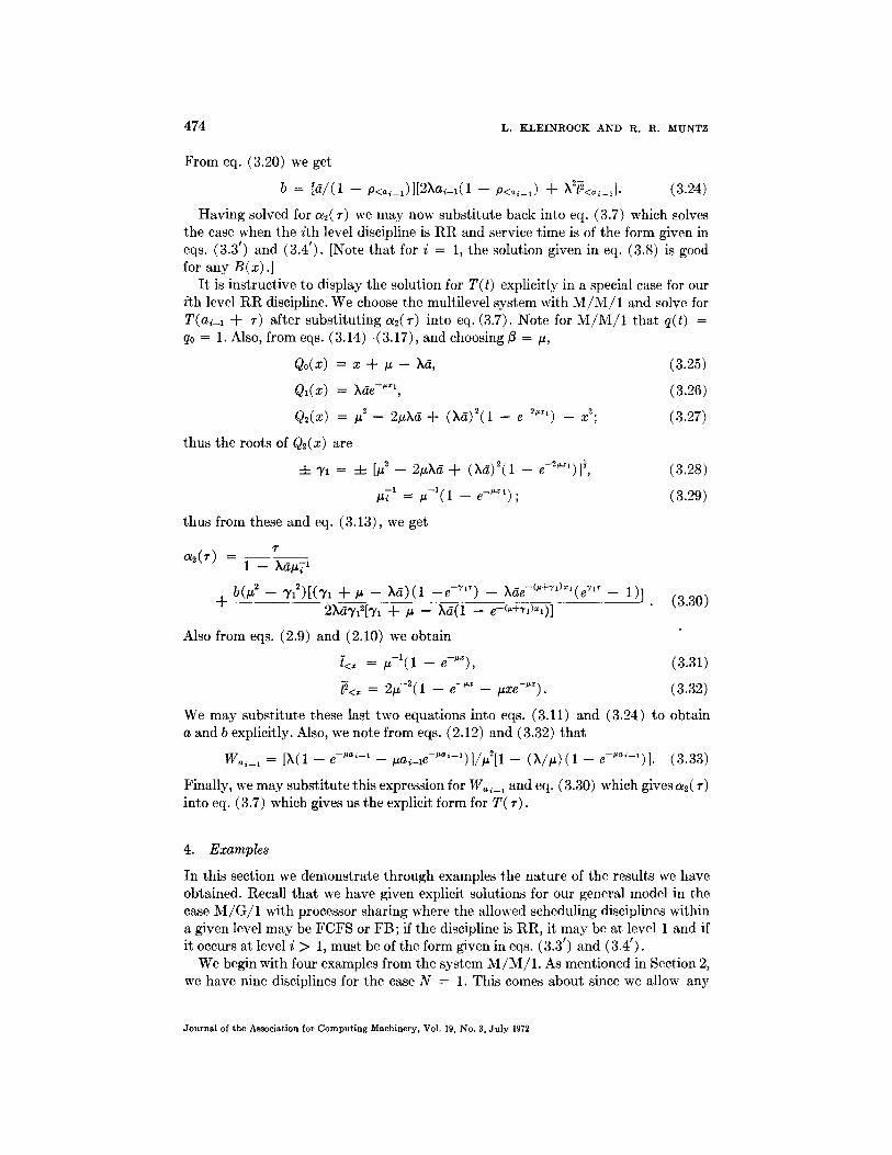
o n e o£ three disciplines at level 1 and any one of three disciplines at level 2. As we have shown, the behavior of the average conditional response t ime in any particular level is independent of the discipline in all other levels; thus we have nine disciplines. In Figure 5 we show the behavior of each of the nine disciplines for the system N = 1. In this case we have assumed ~ = 1, X = 0.75, and al = 2. From eq. (3.1) we see that the response t ime for the FB system is completely independent of the values a~ and therefore the curve shown in Figure 5 for this response t ime is applicable to all of our M / M / 1 cases. Note the inflection point in this curve and tha t the response t ime grows linearly as t --~ ~ [a phenomenon not observable from previously published figures but easily seen from eq. (3.1)]. As can be seen from its defining equation, the response t ime for FCFS is linear regardless of the level; the R R system at level 1 is also linear, but as we see from Figure 5 and from eq. (3.13) the R R at levels i > 1 is
4 0 -
3 6 -
32 -
28 -
2 4 -
20 -
1 6 -
12 -
/ /
/ / i l l
,,:s< 0
/ / FCFS
81
0 ! 0 1
I ~ ' - - -RR
~--FCFS
I I I 2 3 4
t
I I I 5 6 7
FIG. 5. R e s p o n s e t i m e p o s s i b i l i t i e s f o r N = 1, M / M / l , tL = 1, ~ = 0 .75 , a l = 2.
Journal of the Association for Computing Machinery, Vol. 19, No. 3, Ju ly 1972
476 L. K L E I N R O C K AND R. R . MUNTZ
nonlinear. Thus one can determine the behavior of any of nine possible disciplines from Figure 5. Adiri and Avi-I tzhak considered the case (FB, RR) [14].
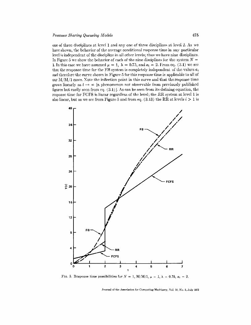
Continuing with the case M / M / l , we show in Figure 6 the case for N = 3 where D1 = RR, D2 = FB, D3 = FCFS, and D4 = RR. In this case we have chosen a~ = i and ~ = 1, k = 0.75. We also show in Figure 6 the case FB over the entire range as a reference curve for comparison with this discipline. Note (in general for M / M / 1 ) tha t the response t ime for any discipline in a given level must either coincide with FB curve or lie above it in the early par t of the interval and below it in the latter par t of the interval; this is true due to the conservation law [15].
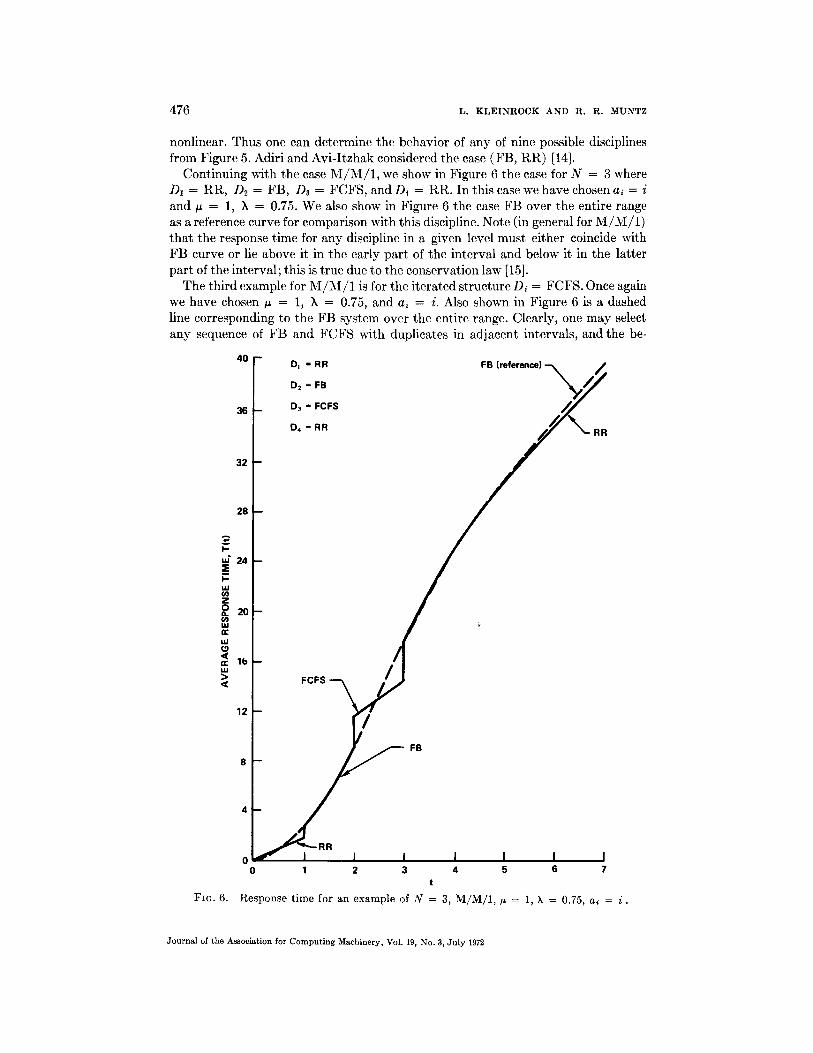
The third example for M / M / 1 is for the i terated structure D i = FCFS. Once again we have chosen ~ = 1, k = 0.75, and ai = i. Also shown in Figure 6 is a dashed line corresponding to the FB system over the entire range. Clearly, one may select any sequence of FB and FCFS with duplicates in adjacent intervals, and the be-
40
32
28
A
I -
u~ 24 :E m p. uJ cn Z =°20 cn Ilc uJ
> <
D: = R R
D2 = FB
D3 = FCFS
04 = RR
FCFS /
FB (reference)
RR
12
FB
FIG. 6.
J I I I I I I 0 0 1 2 3 4 5 6 7
t
R e s p o n s e t i m e f o r a n e x a m p l e o f N = 3, M / M / 1 , / ~ = i , X = 0 .75 , a~ = i .
Journal of the Association for Computing Machinery, Vol. 19, No. 3, Ju ly 1972
Processor Sharing Queueing Models 477
havior for such systems can be found from Figure 7. I t is interesting to note in the general M / G / 1 case with Di = F C F S tha t we have a solution for the FB sys tem with finite q u a n t u m q~ = a~ = a~-z where preempt ion within a q u a n t u m is per- mitted !
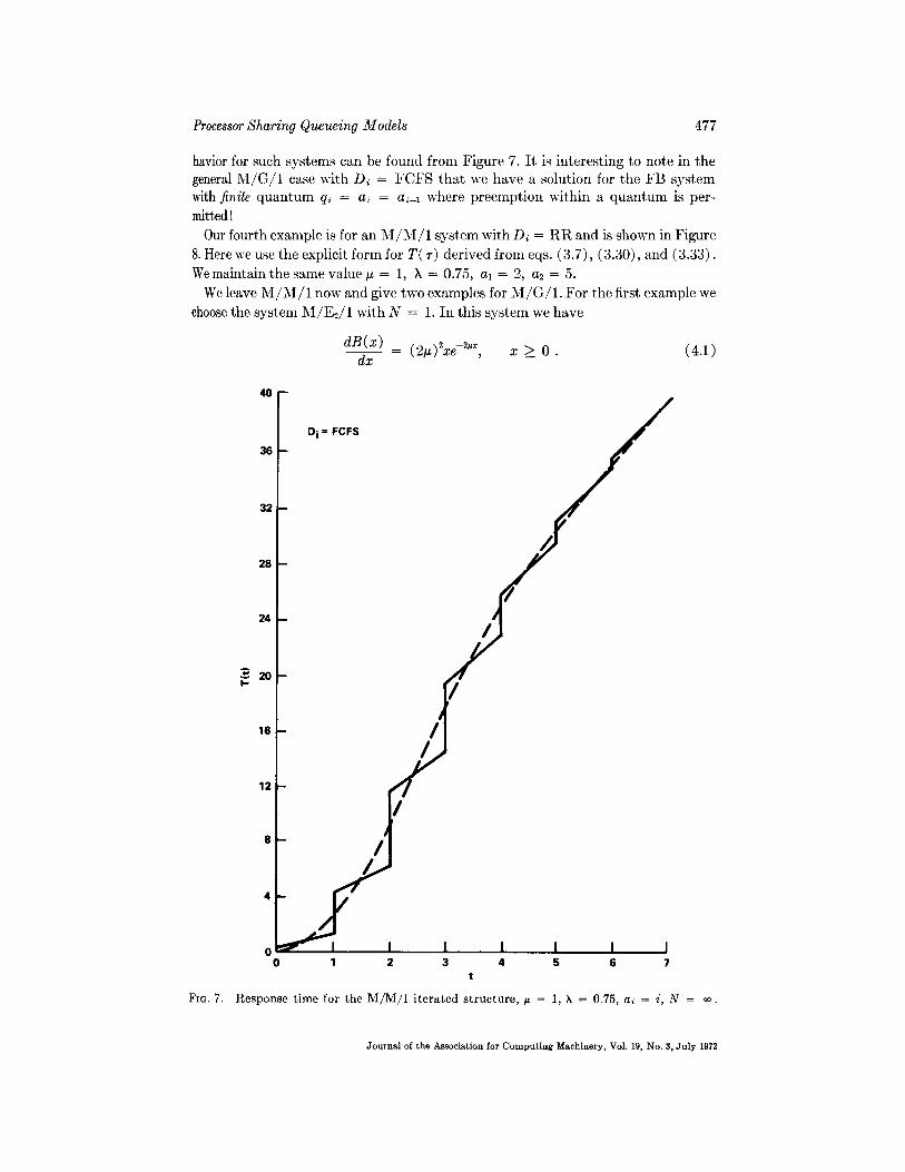
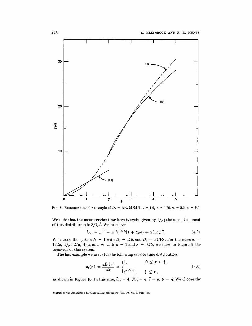
Our fourth example is for an M / M / 1 system with Di = R R and is shown in Figure
8. Here we use the explicit form for T(T) derived f rom eqs. (3.7), (3.30), and (3.33).
We maintain the same value ~ = 1, k = 0.75, a l = 2, a2 = 5.
We leave M / M / 1 now and give two examples for M / G / 1 . For the first example we
choose the system M / E 2 / 1 with N = 1. I n this system we have
dB(x) - (2~)2xe -~x, x ~_ 0 . (4.1)
dx
40
36 L Di = FCFS
32
28
24
L20
/
16~
12
/
FIG. 7.
o l , ~ ,- t t I L I I I 0 1 2 3 4 5 6 7
t
R e s p o n s e t i m e fo r t h e M / M / 1 i t e r a t e d s t r u c t u r e , t~ = 1, k = 0.75, a l = i , N = ~ .
Journal of the Association for Computing Machinery, Vol. 19, No. 3, July 1972
478 L. K L E I N R O C K AND R. R. MUNTZ
A
I - -
30
20
10
I I I I t
/
FB - ~ / /
/ / / ~ RR
__ / 7
I I
I I
i /
i I R
I J J i i 0 1 2 3 4 5
FIG. 8. Response time for example of D~ = RR, M/M/1, ~ = 1.0, ~ = 0.75, a~ = 2.0, a~ = 5.0.
We no te t h a t the mean service t ime here is aga in given by l / p ; t he second moment of th is d i s t r i bu t i on is 3/2~ 2. W e calcula te
/<al = /z -1 - /-t-le-2"al[1 + 2~ai -t- 2(~al)2]- (4.2)
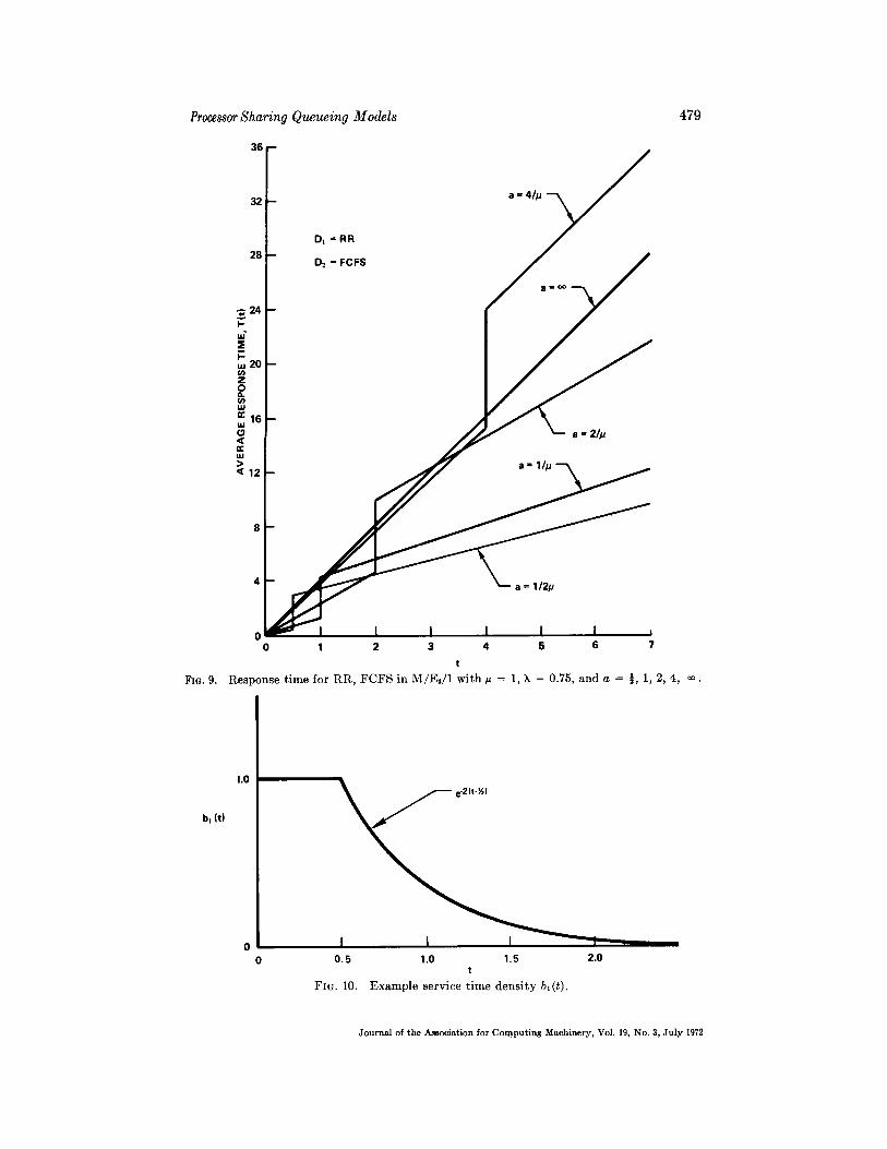
We choose the sys tem N = 1 wi th D1 = R R and D2 = F C F S . F o r t he cases a~ = 1/2~, I/p, 2/~, 4/~ , and ~ wi th # = 1 and k = 0.75, we show in F i g u r e 9 the behav io r of th is sys tem.
The las t example we use is for the fol lowing service t ime d i s t r ibu t ion :
b~(x) dB,(z) I 1' 0 _< x < ½, - - - ( 4 . 3 )
dx (e -2(x-~), ½ ~ X ,
as shown in F igure 10. I n th is case, [<~ = 9, ~<t = ~, [ = 9, ~ = 9. W e choose the
Journal of the A~sociation for Computing Machinery, Vol. 19, No. 3, July 1972
Processor Sharing Queueing Models 479
bl (t)
36 --
32 - a = 4//J " - ~ t /
Di =RR
28 - D2 = FCFS Z = ~ /
0 1 2 3 4 5 6 7 t
Res ~onse t ime for RR, F C F S in M / E : / 1 wi th p = 1, ~ = 0.75, and a = ½, 1, 2, 4, ¢~.
1.0 . . 1
Fro. 9.
0 I I I I 0 0.5 1.0 1.5 2.0
t FIG. 10. Exa mple service t ime dens i ty bl(t).
Journal of the Association for Computing Machinery, Vol. 19, No. 3, July 1972
5 .0
4.0
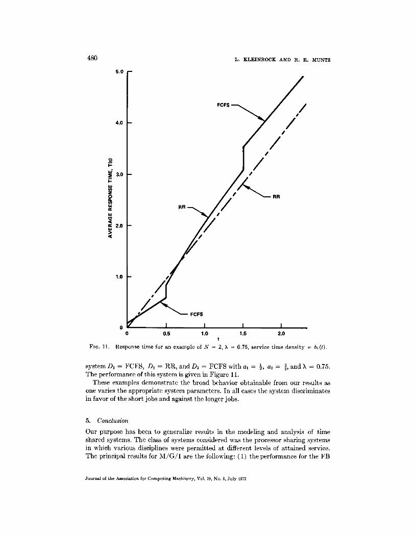
FIG. 11.
FCFS
A
I -
3.0 I - I,li/
Z
r3 <
iJJ > <
2.0
1.0
480 L. K L E I N R O C K AND R. R. MUNTZ
/
/
B
L ~ j ~ F C F S j I I 0.5 1.0 1.5 2.0
Response time for an example of N = 2, ~ = 0.75, service time density = bl(t).
system D1 = FCFS, D2 = RR, and D3 = FCFS with a] = ½, a2 = ~, and k = 0.75. The performance of this system is given in Figure 11.
These examples demonstrate the broad behavior obtainable from our results as one varies the appropriate system parameters . In all cases the system discriminates in favor of the short jobs and against the longer jobs.
5. C o n c l u s i o n
Our purpose has been to generalize results in the modeling and analysis of t ime shared systems. The class of systems considered was the processor sharing systems in which various disciplines were permit ted at different levels of attained service. The principal results for M / G / 1 are the following: (1) the performance for the FB
Journal of the Association for Computing Machinery, Vol. 19, No. 3, July 1972
Processor Sharing Queueing Models 481
discipline at any level is given by eq. (3.1); (2) the performance for the FCFS discipline is linear with t within any level and is given by eq. (3.2); (3) the per- formance for the RR discipline at the first level is well known [8] and is given by eq. (3.8) ; (4) an integral equation for the average conditional response time for RR at any level (equivalent to bulk arrival RR) is given by eq. (3.12) and remains un- solved in general; however, for the service distribution given in eqs. (3.3') and (3.4'), we have the general solution given in eq. (3.13) as derived in [11]. We further note that the average conditional response time at level i is independent of the queueing discipline at all other levels.
Examples are given which display the behavior of some of the possible system configurations. From these, we note the great flexibility available in the multilevel systems. From the examples in Section 4, we see that considerable variation from previously studied algorithms is possible so long as the number of levels is less than a small integer (say 5) ; however, we see that as N increases, the behavior of the ML systems rapidly approaches that of the pure FB system.
Examination of the envelope of the multitude of response functions available with the ML system has suggested that upper and lower bounds in system performance exist; this in fact has been established and is reported in [19].
REFERENCES
(Note. Reference [10] is not cited in the text.)
1. KLEINROCK, L. Analysis of a time-shared processor. Naval Res. Logistics Quart. 2, 1 (March 1964), 59-73.
2. McKINNEY, J . M . A survey of analytical t ime-sharing models. Comput. Surv. 1, 2 (June 1969), 105-116.
3. TAK~CS, L. A single-server queue with feedback. Bell System Tech. J. 42 (March 1963), 505-519.
4. KLEINROCK, L. Time-shared systems: A theoretical t reatment. J. ACM 14, 2 (Apr. 1967), 242-261.
5. COFFMAN, E. G., AND KLEINROCK, L. Feedback queueing models for time-shared sys- tems. J. ACM 15, 4 (Oct. 1968), 549-576.
6. COFFMAN, E. G., JR., MUNTZ, R. R., AND TROTTER, H. Waiting time distributions for processor-sharing systems. J. ACM 17, 1 (Jan. 1970), 123-130.
7. KLEINROCK, L., AND COFFMAN, E. G. Distr ibution of at tained service in time-shared systems. J. Comput. Systems Sci. 8 (Oct. 1967), 287-298.
8. SAKATA, M., NOGUCHI, S., AND OIZUMI, J. Analysis of a processor-shared queueing model for time-sharing systems. Proc. 2nd Hawaii Internat . Conf. on System Sciences, Jan. 1969, pp. 625-628. SCHRAGE, L . E . The queue M/G/1 with feedback to lower priority queues. Manag. Sci. 13, 7 (1967), 466-471. CONWAY, R. W., MAXWELL, W. L., AND MILLER, L . W . Theory of Scheduling. Addison- Wesley, Reading, Mass., 1967. KLEINROCK, L., MUNTZ, R. R., AND RODEMICH, E. The processor-sharing queueing model for time-shared systems with bulk arrivals. Networks J . 1,1 (1971), 1-13. COHEN, J. The Single Server Queue. Wiley, New York, 1969. OLIVER, R. M., AND JE~'ELL, W. S. The distribution of spread. Research Report 20, Op. Res. Cen., U. of California, Berkeley, Calif., Jan. 25, 1962. ADIRI, I., AND AVI-ITZHAK, B. Queueing models for time-sharing service systems. Tech- nion, Mimeograph Ser. on Oper. Res., Statist . and Econ., Technion--Israel Inst. of Teehnol., Haifa, Israel, No. 27.
9.
10.
11.
12. 13.
14.
Journal of the Association for Computing Machinery, Vol. 19, No. 3, July 1972
482 L. KLEINROCK AND R. R. MUNTZ
15. KLEINROCK, L. A conservation law for a wide class of queueing disciplines. Naval Res. Logistics Quart. 12, 2 (June 1965), 181-192.
16. KLEINROCK, L., AND MUNTZ, R. R. Multilevel processor-sharing queueing models for time-shared systems. Proc. Sixth Internat. Teletraffic Congress, Munich, Germany, Aug. 1970, pp. 341/1-341/8.
17. GAVER, D. Diffusion approximations and models for certain congestion problems. J. Appl. Prob. 5 (1968), 607--623.
18. SCHRAGE, L . E . Some queueing models for a time-shared facility. Ph.D. dissertation, Dept. of Indust. Eng., Cornell U., Ithaca, N.Y., 1966.
19. KLEINROCK, L., MUNTZ, R. R., AND HSU, J. Tight bounds on the average response time for processor-sharing models of time-shared computer systems. Proc. IFIPS Congress, 1971 (to be published).
RECEIVED SEPTEMBER 1970; REVISED AUGUST 1971
Journal of the Association for Computing Machinery, Vol. 19, No. 3, July 1972
A Stochastic Model for Message Assembly Buffering with
a Comparison of Block Assignment Strategies
GARY D. SCHULTZ
IBM Research Division, Research Triangle Park, North Carolina
ABSTRACT. A stochastic model is developed for the process of dynamic buffering for inbound messages in a computer communications system. For a specific characterization of message traffic, complementary viewpoints--one considering the process as a queueing system, the other considering it as a compound process--lead to the same probability generating function. Two buffer assignment schemes, both dynamic but differing in binding strategy, are compared in terms of optimal buffer size and total buffer pool requirements for a given overflow criterion. A simple model of optimal blocking, earlier proposed by Gaver and Lewis, is extended to cover both buffer strategies and also heterogeneous message sources. Finally, the derived characteri- zation of total storage requirements is compared by numerical example with conservative and nonconservative asymptotic treatments of the process.
KEY W O R D S A N D PHRASES: buffer assignment schemes, buffer block binding, computer com- munications model, dynamic buffer allocation, geometric binomial distribution, geometric Poisson distribution, message assembly buffering, optimal buffer size, Pdlya-Aeppli distribu- tion, shared buffer storage
CR CATEGORIES; 3.81, 4.39, 5.5, 6.29
Introduction
A design problem of interest arising in computer communication systems concerns the technique employed at the centralized computer facility for buffering inbound messages from a number of communication lines. Static assignment of private storage to each line for message assembly results in costly and inefficient usage of the memory resource by ignoring the stochastic behavior of both message genera- tion and message length. Thus it is commonplace for system designers to capitalize on the orders of magnitude disparity between computer processing speed and line transmission rate and share buffer storage among all the lines by dynamically al- locating buffers from a public pool during the message assembly process.
Such dynamic buffering techniques have the usual characteristic that the public pool is segmented into buffer blocks of equal size. As a message arrives at the com- puter, it is assembled by hardware and software intervention into (generally) non- contiguous blocks allocated piecemeal from the pool. This scatter assembly of a message imposes a storage penalty per block for chaining information to preserve the logical integrity of the data structure.
In this paper we establish means for determining optimal buffer block size and
Copyright © 1972, Association for Computing Machinery, Inc. General permission to republish, but not for profit, all or part of this material is granted, provided that reference is made to this publication, to its date of issue, and to the fact that reprinting privileges were granted by permission of the Association for Computing Machinery. Author's address: IBM Corp., P.O. Box 12275, Research Triangle Park, NC 27709.
Journal of the Association for Computing Machinery, Vol. 19, No. 3, July 1972. pp. 483-495.
4 8 4 G . D . SCHULTZ
total storage requirements for two buffer assignment schemes, both dynamic but differing in binding strategy. The differences in strategy roughly typify the varying performance constraints imposed by imbedding the line handling function within a high supervisory overhead, general purpose control program, or by placing it in a low overhead, dedicated subsystem characterized by a special purpose front end processor.
To facilitate comparison, we study the inbound message storage process in vacuo, formulating a stochastic model of storage usage with specific distributions imposed on message generation and message length. An interesting study of buffering by Gaver and Lewis [1] is cited, both because their approach somewhat parallels this one and because a simple blocking model they proposed lends itself to generalization and extended application here. They considered the low overhead buffering scheme in more generality with respect to distributional assumptions, and proposed a buf- fer storage performance criterion based on rate of exceeding buffer limits. Here we develop a model using more restrictive message traffic assumptions, but carry through the analysis of storage overflow without appeal to asymptotic approxima- tions based on the central limit theorem.
Modeling Storage Usage
Consider a computer facility having M communication lines attached. To develop a model of storage usage for message assembly, we make the following assumptions about the input process:
(1) Each of the M lines feeding the computer has identical characteristics, with activity on one line being independent of activity on any other.
(2) Arrival of individual characters belonging to a single message proceeds at a constant rate (r characters per second) from start of message (SOM) through end of message (EOM).
(3) Each line experiences alternating periods of activity and inactivity. Consider- ing the combined process as comprised of two alternating sequences of independent random variables, we describe both by exponential probability distribution func- tions with parameters # (activity) and X (inactivity). Thus, mean message trans- mission time is 1/#, while the mean time between EOM and SOM is 1/X.
We are interested in comparing two buffer assignment schemes, described as fol- lows.
Scheme 1. A buffer block is assigned instantaneously at the time of its immediate need, e.g. when the first character to enter the block begins to arrive. We call this scheme incremental block binding (IBB).
Scheme 2. One buffer block is preassigned to each line. During an active period, a new buffer block is allocated one "block time" prior to its (potential) need, e.g. when the first character to enter the most recently assigned buffer block begins to arrive. We call this scheme anticipatory incremental block binding (AIBB).
In general, the IBB scheme is possible where little overhead is incurred for per- forming block allocation, while the AIBB scheme characterizes higher overhead systems [2]. "Instantaneous" block assignment is, of course, a mathematical idealization, but it is realistic when considering the transmission rates of commonly used communication lines. Thus, in typical real systems, "high" overhead may en- tail only a significant fraction of a single character time.
Journal of the Association for Computing Machinery, Vol. 19, No. 3, Ju ly 1972
Stochastic Model for Message Assembly Buffering 485
Two approaches which give complementary insights into the process are sug- gested. One approach considers the process as a queueing system, while the other conceives it as a compound process. In either case we are interested in the process in equilibrium; that is, we want the probability distribution for the number of storage blocks currently assigned at an arbitrary time, t, to be sufficiently removed from a "zero time" so that any initial condition effects (e.g., all lines idle) have '<worn off,"
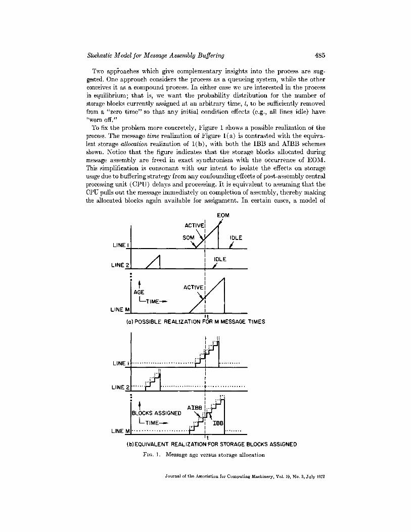
To fix the problem more concretely, Figure 1 shows a possible realization of the process. The message time realization of Figure l(a) is contrasted with the equiva- lent storage allocation realization of l (b) , with both the IBB and AIBB schemes shown. Notice that the figure indicates that the storage blocks allocated during message assembly are freed in exact synchronism with the occurrence of EOM. This simplification is consonant with our intent to isolate the effects on storage usage due to buffering strategy from any confounding effects of post-assembly central processing unit (CPU) delays and processing. It is equivalent to assuming that the CPU pulls out the message immediately on completion of assembly, thereby making the allocated blocks again available for assignment. In certain cases, a model of
EOM I
ACTIVEI A ~ s° t LINE I f
I
A ' I IDLE i / L INE2 I
: i I
i 2 AcT,vE,J
AGE I
L~TiME-....
LINE M i t
(a} POSSIBLE REALIZATION FOR M MESSAGE TIMES
.... • .... ° ........ .°.. o . , , , ~ ..... . .... L NEI LINE 21 . . . . . . . . . . . . . . . . . . . . . . . . . . t . . . . . . . . . . . . . . . . . I
• i . . . • | . . .
I I ' . - A I B B I:": BLOCKS ASSIGNED ~hJ :" " ~
LINE M ................... t
(b)EQUIVALENT REALIZATION FOR STORAGE BLOCKS ASSIGNED
FzG. l. Message age versus storage allocation
Journal of the Association for Computing Machinery, Vol. 19, No. 3, July 1972
486 G.D. SCHULTZ
storage usage that goes beyond the message assembly considerations modeled here may also justifiably neglect post-assembly effects. For example, CPU processing may be negligible compared to message transmission t ime--a frequent case in prac- tice. Alternatively, post-assembly processing may take place in work space inde- pendent of the buffer pool following high priority CPU transfer of the message out of the buffer blocks at EOM time.
From Figure l(b) it is also clear that the AIBB scheme simply adds M blocks to that required for IBB. Thus, as far as storage usage is concerned, we can develop a model for both by treating the IBB scheme and extending it to AIBB in a simple fashion. This approach is used in the following derivation.
I t is convenient to conceive of the entire process as consisting of M independent M / M / 1 queueing systems (Poisson arrivals, exponential service, single server) where "service t ime" corresponds to the interval between SOM and EOM (message length). By defining each to be a pure loss system with no waiting room at the server, we can choose the same parameters (h, tt) as given by our earlier assump- tions to get a mathematically equivalent characterization. Since the distribution of the time between two consecutive Poisson points (SOMs) is the same as the distri- bution of the time between an arbitrary point (e.g. EOM) and the next Poisson point (SOM), the lossy aspect upholds the earlier assumption (3) and allows us to ignore the unreal possibility of multiple messages queued on a single line. By the independence assumption, a one-line model extends easily to the M-line process.
For an M / M / 1 queueing system with a maximum of one in the system (i.e. the one in service), it is known [3] that in equilibrium:
Pr {system is idle}
Pr {system is busy}
where p = k/#.
= Pr {zero customers in the system}
= 1/ (1 + p)
= p / (1 + p)
(1)
(2)
We can use these results first to derive the equilibrium probability for the "age" or elapsed service time of the message (if one) active at an arbitrary time t, and then to obtain the probabilities for the number of storage blocks currently assigned to the line (using assumption (2)). Defining the random variables M a ( t ) as the message age at time t, and M s ( t ) as the (discrete) number of buffer blocks assigned at time t, we get
Pr {Ma(t) = 0} = Pr {system idle} = 1/(1 + p) = Pr {M,(t) = 0}. (3)
The presence of a message of age v > 0 at time t means that at time t - v the line changed from idle to active by the arrival of SOM, and the resulting message has length at least as great as v. This is more precisely stated in differential notation as:
Pr {v < M a ( t ) < v + dr} = Pr {line idle at time t - - v - - dr}
• Pr {SOM occurs in ( t - v - - dr , t - v)} • Pr {message length > v}
= 1/(1 + p).X d v . e - ~ (4)
where the parameters are as defined in assumption (3). To get the probability for the number of blocks assigned, we first define buffer block size B = b + c, where c is the number of storage spaces needed for chaining and b is the number of spaces
Journal of the Azmoclation for Computing Machinery, Vol. 19, No. 3. July 1972
Stochastic Model for Message Assembly Buffering 487
available to receive message characters. Then, using assumption (2) of constant character rate, r, and defining 1/a = b/r, we use eq. (4) to get for y = 1, 2, . . . ,
Pr {Ms(t) = y} = P R E Y - 1 < M = ( t ) < Y-~ ( a a )
- 1 ~ p J(~-l)/= e-~v dv
- P (1 - e-"/~)e -(~-1)~/~. (5) l ~ p
The integration in (5) is a consequence of the fact tha t exactly y discrete blocks are assigned from the instant that y - 1 have completely arrived through the instant that the yth block is completely filled. Notice that for y = 1, 2, • • • ,
Pr {Ma(t) = y [ system busy} = (1 - e-~/~)e -(~-1)~/= (6)
and is zero otherwise. This is the geometric distribution with parameter e -~/=. Thus, using eqs. (3) and (5), the probability generating function, P(s) , for the
single-line process is
1 + ~ P ( 1 - p) p~-ls~ (p = e -~/~) P ( s ) - 1 +----p ~=~ 1 + p
= (1 -- ps + ps -- pps ) / (1 + p)(1 -- ps) (7)
and the probability generating function, H(s ) , for the M-line process becomes
H ( s ) = [P(s)l M [.1 -- ps W ps -- ppslU
The queueing theory approach has the advantage that the variables of buffer size, message length, and line speed enter naturally into the treatment. Insights gained from a complementary viewpoint, however, permit more natural derivation of the desired probability distribution and also provide the basis for discussion, in a later section of the paper, of asymptotic processes.
Viewing the total process in equilibrium, then, as a compound process [4], we can relax the assumption on message (SOM) generation, and simply take the event of finding a line active as the outcome of a Bernoulli trial, with activity having prob- ability Q. In this case, we are interested in the sum SN(t) of a sequence {Xk(t)} of mutually independent random variables with the common distribution Pr {Xk(t) ---- i} = f~ and generating function F(s) = Z f y . The number N(t ) of terms in the sum SN(t) is also a random variable independent of the Xk(t) with distribution Pr {N(t) = n} = g, and generating function G(s) = Zg, s". For the distribution hi} of So(t) we get
M
~, = Pr {So(t) = i} = ~ e r {N(t) = n} e r {X,(t) + . - . + X , ( t ) = i}. (9) n~0
in terms of our process in equilibrium, we let N(t ) correspond to the number of tctive lines, and Xk(t) correspond to the number of buffer blocks currently assigned o the kth active line. To preserve the discrete nature of storage allocation, we Lscribe to Xk(t) the geometric distribution with parameter p. Then
f , = p J - l ( 1 - p), j = 1 , 2 , . . . , (10)
Journal of the Association for Computing Machinery, Vol. 19, No. 8, July 1979
488 G.D . SCHULTZ
g, = (nM) Q " ( 1 - Q) M-", n = 0 , 1 , - . - , M . (11)
For a fixed n, the distribution of Xi(I) + .. • + X,( t) is given in Feller's notation [4] by {fj}"*, the n-fold convolution of {f~.} with itself, giving
M
{h , } = g.{f,}"*. (12) n~0
With
and
F(s) = ~ p~-1(1 -- p)s j - s(1 -- p) .i~1 1 - - ps
(13)
G(s) = ~ ( ~ ) Q " ( 1 - Q)M-"s"= ( 1 - (14)
we find the generating function of the sum SN(t) to be
H(s) = his' = ~ g,[F(s)l" i =0 n =0
s(1 - p ) l = G(F(s)) = 1 -- Q + Q ~ _~-p-~.j
[ 1 - ps - Q W Qs] M = 1 p s ' (15)
which, with p = e - ' /" and Q = p/(1 + p), agrees with (8). To get the distribution, we make use of eq. (9) to derive for the zero term:
h0 = P r { N ( t ) = 0} = ( 1 - Q)M. (16)
Using (13) we find
[F(s)] n = (1 - p)%"(1 - ps) -n
= ( 1 - - P ) " S ' ~ ( ~ n ) ( - p s ) k k ~ o
= (1--p) 's '~(n+k-- 1) k (17)
Thus
= - - p , i _ > n
and is zero for i < n. Substituting this result, along with that of eq. (11), into eq. (12) we get for i _> 1,
h, = (1 -- Q)Mp, ~__, . (19)
Conforming with conventions [5] for other compound processes, we call the distribu- tion defined by (16) and (19) the geometric binomial distribution. Knowing H(s)
.Journal of the Association for Computing Machinery, Vol. 19, No. 3, July 1972
Stochastic Model for Message Assembly Buffering 489
(or, see [4], using G(s) and F ( s ) ) allows us to derive the mean and second and third central moments for So(t). Using conventional notation, where t~', is the rth moment (about zero) and ~, is the rth central moment, these are:
t*l' = M Q / ( 1 - p) , (20)
#2 = M Q ( 1 + p - 0 ) / ( 1 - p)~, (21)
tt3 = MQ[(2Q - 1 - p ) ( Q - 1 - p) + 2p]/(1 - p)3. (22)
Suppose, then, that the concern is to choose ~ finite buffer pool size such that for given parameters some performance criterion is to be met. An obvious approach is to consider the finite storage process to be well characterized by the unconstrained process modeled above. In this case, choosing probability of over,flow as a criterion, for the idealized process we simply find a storage level whose probability of being exceeded matches the overflow criterion. The shortcoming in this matching is inherent in the departure of the real, finite storage process from the unconstrained mathematical idealization at the storage boundary. In actual systems, all blocks assigned to an overflowing message are immediately released at the time of over- flow, causing congestion to fall below the critical point. An additional complica- tion is the twofold perturbation in the input process at the boundary due to effective idleness of the source of the violating message until EOM and the subsequent retransmission event. These effects, as well as second order performance criteria based on refined analysis of the unconstrained process as treated (asymptotically) in [1], are ignored here since they are not crucial to the comparison of buffering schemes. For the purposes of the present study, probability of overflow remains an apt first order performance criterion.
Applying such a criterion, eqs. (16) and (19) can be used to find a level S, say, such that Pr {Sic(t) > S} < e or, equivalently, Pr {SN(t) < S} >_ 1 - e, where e is the performance constraint. This yields the number of blocks required in the finite pool to satisfy requirements. For the IBB buffering scheme, the pool consists of S. B characters while, for AIBB, (S Jr M) • B characters comprise the pool.
If buffer pool blocking did not incur a chaining penalty, and if system over- head for dynamic block allocation were not at issue, it is obivous that a one-character block size should be chosen to minimize total storage requirements. The fact that block size, B = B + c, involves a chaining field which is not available for reception of message characters introduces an apparent tradeoff. With too small a block size, a large portion of the pool is devoted to space for chaining fields; while with too large a block size, the earlier binding of available storage lowers the efficiency of storage usage. The latter effect is particularly acute for the AIBB scheme, where an available buffer dangles unused an entire "block t ime" (b character times) prior to its actual use for incoming characters. Both schemes suffer from an approximate additional half block time early binding per allocated character (on the average) while the block is being filled.
Finding a block size that minimizes overall storage requirements is relatively simple. Holding all other parameters fixed, eqs. (16) and (19) are used with b
n b varying. For each b, we can find the smallest n~ such that S(nb) = ~ i = 0 h l >_ 1 - e, where e is the overflow constraint. Multiplying nb by B, or ( n b + M) by B, gives the total buffer pool size in characters for the IBB and AIBB schemes,
Journal of the Association for Computing Machinery, VoL 19, No. 3, July 1972
490 G.D. SCHULTZ
FIG. 2.
70,000
60,000
(/1
50,000 ,¢
U
W _N (D j 40,000 0 0 0. Q
°w 30,000 I.i,I Z
20,000
~ i ~ b o p l PREDICTED FOR A I B B
bopt PREDICTED FOR IBB
J AIBBJ"
.~..,fs././ M= I00
o~
xl'... - I BB """
i i
AIBB " ~ "
AIBB M=IO ,
Q= .5 r --= 600
C=4 E= .01
I0,000 "%~==:=~_:
I IBS I I i i l
50 I00 150 200 b
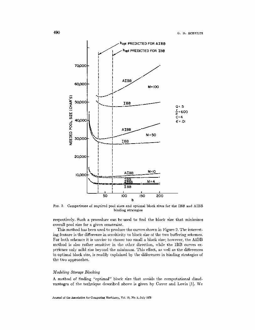
Comparisons of required pool sizes and optimal block sizes for the IBB and AIBB binding strategies
respectively. Such a procedure can be used to find the block size that minimizes overall pool size for a given constraint.
This method has been used to produce the curves shown in Figure 2. The interest- ing feature is the difference in sensitivity to block size of the two buffering schemes. For both schemes it is unwise to choose too small a block size; however, the AIBB method is also rather sensitive in the other direction, while the IBB curves ex- perience only mild rise beyond the minimum. This effect, as well as the differences in optimal block size, is readily explained by the differences in binding strategies of the two approaches.
Modeling Storage Blocking A method of finding "optimal" block size that avoids the computational disad- vantages of the technique described above is given by Gaver and Lewis [1]. We
Journal of the Association for Computing Machinery, VoL 19, No. 3, July 1972
8tochastic Model for Message Assembly Buffering 491
generalize their model here to encompass the AIBB scheme as well as the IBB method, and we also extend it by temporarily relaxing the assumption that all lines must be identical.
Begin by considering an individual line i. Suppose on this line the average message length is Ii, while the average line loading, or fraction of time the line is active sending characters, is Q~. While the line is inactive, there are ~ storage spaces wasted for buffering, where/3 = 0 (IBB) or ~ = b + c (AIBB). While the line is active, the number of storage spaces wasted (assignedj but not holding characters) will vary according to the current age, or elapsed service time, of an observed inbound message. The relationship between average message length, l~, and the average ob- served age, denoted m; , of an inbound message (both in character times) is apparent using results (not dependent on the exponential distribution assumption) from [6] for "backward recurrence time," e.g. mi 7( i + z~/li), where ai 2 is the variance of message length for line i. In the specific case of the exponential distribu- tion, where the mean and standard deviation of message length are equal, m~ = l~.
During activity, then, the expected number of wasted spaces is equal to the scheme-dependent wastage, defined by ~ above, plus the expected wasted spaces in the blocks previously filled and the block currently receiving characters. Includ- ing the previously filled blocks as well as the block currently receiving characters, there are an expected c. I-mi/b"l used for chaining, where [-xq denotes the smallest integer greater than or equal to x (the ceiling of x). For m~ large with respect to b, this is approximately cm~/b. By the same assumption, there are also on average approximately b/2 storage spaces vacant in the buffer block currently being filled. Hence the expected wasted space for line i is
L,(b) = Q~ + -~- + 13 + (1 - Q,)I~. (23)
Considering all lines, the expected total wasted space is M
i (b) = ~ L , ( b ) . (24) i ~ 1
Differentiation with respect to b reveals that L is minimized at
~c + [2c~m~Qi/ZQi] ~ (IBB) (25) Bopt tc + [2cZm~Q~/(ZQ~ + 2M)] ½ (AIBB) (26)
where Bopt = C + bo,t • For homogeneous lines, i.e. mi = m (because Ii = l and zi = ~) and Qi = Q
(i = 1, 2, . . . , M), we get
+ [2cml' (roB) (27) Bop~ + [2cmQ/(Q + 2)] t (AIBB). (28)
The result in (27) agrees with that given by Gaver and Lewis in [1] where a further refinement of their model, focussing on loss in the last utilized block and using the distribution function of message length, is posed to show the quality of the approximation leading to (27). The utility of the above model is illustrated in Figure 2, where the optimal block sizes predicted by (27) and (28) are indicated.
It is interesting to compare the two buffering schemes with respect to CPU over- head for chaining operations. Let C i denote the expected chaining overhead (num- ber of chaining interrupts) per message for scheme i where the superscript i = 1
Journal of the ~s,qociation for C o r n n u t l n c , M ~ n h ; ~ r ~ V ~ I 10 N.T~ ~ ?,.1.. 10~0
492 G.D. SCHULTZ
(IBB) or 2 (AIBB). For each scheme we assume that the pool is optimally blocked, 1 2 • with bopt and bopt denoting the optimal values found for IBB and AIBB, respectively.
Then for l, m, c, and Q defined as above:
C 2 _ [l/bo2pt] + 1 _ 1/[2cmQ/(Q + 2)] t + 1
C 1 l/bolpt l/[2cm] i
(2cm ' = (Q + , z2, (29)
In the case of the exponential distribution, where l = m,
C-- i ~ for l >> c. (30)
Asymptot ic Processes
Computational considerations, as evidenced by the complexity of eq. (19), com- monly lead modelers to seek approximation by a more tractable asymptotic process. I t is interesting to contrast the results obtainable from the exact forms derived earlier for the modeled process with results using asymptotic characterizations. Two such approaches, one conservative in approximating storage needs and one non- conservative, are as follows.
A nonconservative approximation results from the assumption that the M-line process can be characterized as asymptotically Gaussian in distribution. From our earlier characterization of the M-line process as a compound process, with total storage allocated being the random sum of mutually independent random variables, we note that, for M sufficiently large, a central limit theorem effect applies [7]. Thus we can simplify computation by choosing a normal distribution, with mean and variance the same as for the actual distribution, to characterize the storage process. For a given overflow constraint, e, this approach approximates the total buffer pool requirement, T, by (in storage blocks)
T = /21 ! ~ ~ 1 - , ~2 ] (31)
whe re / a ' and #2 are given by eqs. (20) and (21), and 51-~ is the deviation found from a standardized normal distribution table such that 1 - e of the distribution lies to its left.
A conservative approximation, on the other hand, results from the assumption that the number of active lines N ( t ) with distribution given by eq. (11) can be asymptotically characterized by the Poisson distribution. Thus, with c~ = M. Q,
Pr {Y(t) = n} ~ ~ . e (32)
This leads to characterizing the M-line process by the well-studied geometric Poisson or Pdlya-Aeppli distribution [5], 1 where eqs. (16) and (19) are replaced by
h0 = e -G, ( 3 3 )
p , > 1
1 The first edition of reference [5] contains incorrect versions of eqs. (36)-(38).
Journal of the Association for Computing Machinery, Vol. 19, No. 3, July 1972
Stochastic Model for Message Assembly Buffering 493
TABLE I
Q M TN/TGB TPA/TGB
• 1 4 .61 1 . 0 3
• 1 10 .71 1 . 0 4
.1 50 .87 1.03 • 1 100 •91 1 . 0 2
.5 4 .81 1.15
.5 10 .88 1.12
.5 50 .96 1.07 • 5 100 .98 1 . 0 5
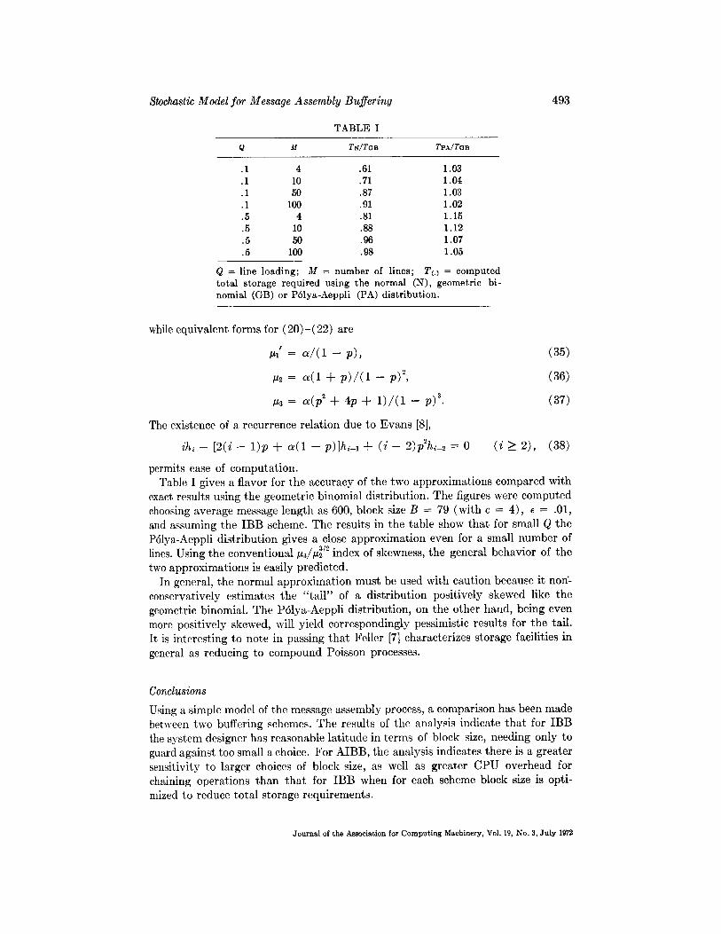
Q = line loading; M = number of lines; T¢.) = computed total storage required using the normal (N), geometric bi- nomial (GB) or P61ya-Aeppli (PA) distribution•
while equivalent forms for (20)-(22) are !
~1 = a / (1 -- p), (35)
~2 = c~(1 + p ) / ( 1 -- p)2, (36)
~3 = c~(P 2 + 4p --b 1) / (1 -- p)3. (37)
The existence of a recurrence relation due to Evans [8],
i h i - [ 2 ( i - 1 ) p + a(1 - p)]h i - l+ ( i - 2)p2hi_2 = 0 ( i > 2), (38)
permits ease of computation. Table I gives a flavor for the accuracy of the two approximations compared with
exact results using the geometric binomial distribution. The figures were computed choosing average message length as 600, block size B = 79 (with c = 4), ~ = .01, and assuming the IBB scheme. The results in the table show that for small Q the P61ya-Aeppli distribution gives a close approximation even for a small number of
3/2 • lines. Using the conventional ~3/~2 index of skewness, the general behavior of the two approximations is easily predicted.
In general, the normal approximation must be used with caution because it noff- conservatively estimates the "tai l" of a distribution positively skewed like the geometric binomial. The P61ya-Aeppli distribution, on the other hand, being even more positively skewed, will yield correspondingly pessimistic results for the tail. It is interesting to note in passing that Feller [7] characterizes storage facilities in general as reducing to compound Poisson processes.
Conclusions
Using a simple model of the message assembly process, a comparison has been made between two buffering schemes• The results of the analysis indicate that for IBB the system designer has reasonable latitude in terms of block size, needing only to guard against too small a choice. For AIBB, the analysis indicates there is a greater sensitivity to larger choices of block size, as well as greater CPU overhead for chaining operations than that for IBB when for each scheme block size is opti- mized to reduce total storage requirements•
Journal of the Association for Computing Machinery, Vol. 19, No. 3, Ju ly 1972
494 G . D . SCHULTZ
A scheme intermediate in strategy with respect to IBB and AIBB would have obvious appeal for the overhead-encumbered systems. We propose the following.
Scheme 3. To an inactive line assign a smaller "root" block of size d, say. Upon receipt of SOM, allocate a buffer block of (normal) size B from the public pool. Allocate each successive block from the pool when'all but d characters of the cur- rently used block have been filled. We refer to this scheme as rooted incremental block binding (RIBB).
The choice of the size d would depend only on the tolerance demanded by worst- case overhead considerations, which by the earlier remarks regarding character arrival times common to communication lines, implies d ~< B.
Analytical comparison of RIBB with IBB and AIBB is a simple matter and reveals RIBB to have the basic advantages of IBB. Notice that RIBB requires M. d more storage than IBB; hence storage usage curves for RIBB are those of IBB (cf. Figure 2) displaced upward everywhere, for b > d, by the amount M.d. Similarly, in eq. (23), ~ = d for RIBB, giving an optimal block size identical to that for IBB (because d is a constant). Thus, for optimal blocking, the CPU chaining overhead per message for RIBB is about the same as for IBB. An important feature of RIBB is that, like IBB, it is only mildly sensitive to larger choices of block size. This permits the system designer to make tradeoffs in favor of lower overall system overhead for message assembly without experiencing the heavier storage penalty of the AIBB method.
While the assumption on message length distribution in the paper is somewhat restrictive, it is not uncommon for modelers to employ such an assumption. More- over, recent results reported by Fuchs and Jackson [9] show that the geometric distribution (the discrete distribution analog of the exponential distribution) can be reasonably fitted to observed statistics for short average message length systems. Similar measurements for longer average message length systems, characterized by CPU-to-CPU communication or "remote buffered" terminal usage, are not yet available in the literature.
It is hoped that the closed form result obtained herein and the perspective on asymptotic processes will be of use for other models as well as for real world applica- tions where the assumptions used are descriptive.
ACKNOWLEDGMENTS. Thanks and acknowledgment are warmly accorded to Professor V. L. Wallace of the University of North Carolina, for whose class an earlier version of this work was a course paper. Besides originally suggesting the fruitful approach of treating each line as an M/M/1 queue, Dr. Wallace gave encouragement and guidance on matters of notation, style, and perspective, and pointed out some errors in the description.
The interest and discussion provided by Dr. J. Spragins of IBM and J. Whitlock Jr., of the University of North Carolina are also gratefully acknowledged.
R E F E R E N C E S
1. GAVER, D. P., JR., AND LEWIS, P. A . W . Probabil i ty models for buffer storage allocation problems. J. ACM 18, 2 (Apr. 1971), 186-198.
2. IBM CORP. IBM System/360 operating system: Basic telecommunications access method. IBM Form GC30-2004.
Journal of the Association for Computing Machinery, Vol. 19, No. 3, July 1972
Stochastic Model for Message Assembly Buffering 495
3. SAATY, T . L . Elements of Queueing Theory with Applications. McGraw-Hill , New York, 1961.
4. FELLER, W. An Introduction to Probability Theory and Its Applications, Vol. I. Wiley, New York, 1957.
5. JOHNSON, i . L., AND KOTZ, S. Distributions in Statistics: Discrete Distributions. Houghton Mifflin, Boston, 1969.
6. Cox, D . R . Renewal Theory. Methuen, London, 1962. 7. F~LLEH, W. Ann Introduction to Probability Theory and Its Applications, Vol. II. Wiley,
New York, 1966. 8. EVANS, D. A. Experimental evidence concerning contagious distributions in ecology.
Biometrika 40 (1953), 186-211. 9. FUCHS, E., AND JACKSON, P . n . Est imates of distributions of random variables for certain
computer communications traffic models. Comm. ACM 13, 12 (Dec. 1970), 752-757.
RECEIVED APRIL 1971; REVISED SEPTEMBER 1971
Journal of the Association for Computing Machinery, Vol. 19, No. 3, July 1972
An Approach for Finding C-Linear Complete Inference Systems
JAMES R. SLAGLE
National Institutes of Health, Department of Health, Education and Welfare, Bethesda, Maryland
ABSTRACT. An inference system is C-linear complete if it is linear (ancestry filter) complete with top clause C, where C is in the original set of clauses and has suitable satisfiability prop- erties. C-linear completeness is important for two reasons: (1) set-of-support refutation com- pleteness is a corollary of C-linear refutation completeness, and previous computer experiments have indicated that the set-of-support strategy is efficient ; (2) the search for a C-linear deduc- tion can be naturally represented by a goal tree, and good techniques are known for searching such trees. A theorem is proved which provides a fairly general approach which, when given only a ground complete inference system, often yields a (nonground) C-linear complete system. This approach can be combined with a previously presented approach whose object is to re- place some of the axioms of a given theory by a refutation complete system. The object of the combined approach is to replace some of the axioms by a C-linear refutation complete system.
The approach of this paper is applied to six combinations of four inference rules. The rules are ordinary resolution, paramodulation, and two rules which respectively replace the transi- t ivi ty axiom for ~ and the set membership axiom. C-linear refutation complete systems are found from the six combinations. For the case of resolution alone, the stronger C-linear deduc- tion (consequence-finding) completeness is obtained.
KEY WORDS AND PHRASES : theorem-proving, completeness theorems, inference systems, linear deduction, linear refutation, inference rules, resolution principle, paramodulation, transit ivity axiom, set membership axiom, artificial intelligence, deduction, refutation, mathematical logic, predicate calculus.
CR CATEGORIES: 3.60, 3.64, 3.66, 5.21
1. Introduction
T h e purposes of p r o g r a m m i n g a c o m p u t e r to p rove theo rems concern ar t i f ic ial in te l l igence [9], deduc t ion , m a t h e m a t i c s , a n d m a t h e m a t i c a l logic. See [10] for a discussion. The reso lu t ion pr inc ip le [8] is an inference rule used in a u t o m a t e d t heo rem-p rov ing . Wos et al. [15, 16], Al len and L u c k h a m [1], a n d o thers have wr i t t en proof- f inding p r o g r a m s e m b o d y i n g t h e reso lu t ion pr incip le . A l though qui te general , these p r o g r a m s have been so slow t h a t t h e y have p r o v e d on ly a few theo- rems of a n y in te res t .
As a s tep in coping wi th th is p rob lem, a p rev ious p a p e r [10] p re sen ted a fa i r ly genera l a p p r o a c h which, when g iven the ax ioms of some special t heory , of ten yields comple te , va l id , efficient ( in t ime) rules cor responding to some of the given axioms. T h e p resen t p a p e r t akes a n o t h e r s tep. A t he o re m is p roved which p rov ides a fa i r ly
Copyright © 1972, Association for Computing Machinery, Inc. General permission to republish, but not for profit, all or part of this material is granted, provided that reference is made to this publication, to its date of issue, and to the fact that reprinting privileges were granted by permission of the Association for Computing Machinery. Author's address: Heuristics Laboratory, Division of Computer Research and Technology, National Institutes of Health, Bethesda, MD 20014.
Journal of the Association for Computing Machinery. Vol. 19, No. 3, July 1972, pp. 496-516.
An Approach for Finding C-Linear Complete Inference Systems 497
general approach which, when given only a g round complete inference system, often yields a (nonground) C-linear complete system. The object of the approach obtained by combining these two approaches is to replace some of the axioms by a C-linear refuta t ion complete system. I n Sections 6 th rough 8 the approach de- veloped in Sections 3 th rough 5 is applied to six combinat ions of four inference rules. Previously, only two of these systems (resolution [5, 6] and resolution with paramodulation [3]) had been proved C-linear complete.
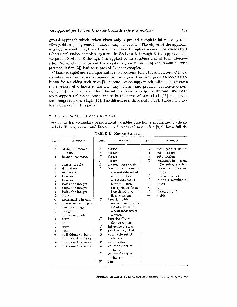
C-linear completeness is impor t an t for two reasons. First, the search for a C-linear deduction can be na tura l ly represented by a goal tree, and good techniques are known for searching such trees [9]. Second, set-of-support refuta t ion completeness is a corollary of C-linear refuta t ion completeness, and previous compute r experi- ments [16] have indicated tha t the set-of-support s t ra tegy is efficient. We mean set-of-support refuta t ion completeness in the sense of Wos et al. [16] and not in the stronger sense of Slagle [ l l] . The difference is discussed in [18]. Table I is a key to symbols used in this paper.
2. Clauses, Deductions, and Refutations
We start with a vocabu la ry of individual variables, funct ion symbols, and predicate symbols. Terms, atoms, and literals are in t roduced next. (See [8, 9] for a full de-
TABLE I. KEg TO SYMBOLs
Symbol Meaning(s) Symbol Meaning(s) Symbol Meaning(s)
a atom, (inference) rule
b branch, constant, rule
c constant, rule d deduction e expression f function g function h index for integer i index for integer j index for integer k literal
m nonnegative integer n nonnegative integer p positive integer q integer r (inference) rule s term t term
u term v term w individual variable x individual variable y individual variable z individual variable
A clause B clause C clause D clause E clause, there exists F function which maps
a countable set of clauses into a countable set of clauses, literal form, clause form, functionally re- flexive axiom
G function which maps a countable set of clauses into a countable set of clauses
H functionally re- flexive axiom
J inference system P predicate symbol Q countable set of
clauses R set of rules S countable set of
clauses T countable set of
clauses W list
u most general unifier 0 substitution r substitution
contained in or equal (for sets), less than or equal (for order- ing)
C is a member of (~ is not a member of U union
not iff if and only if
yields
Journal of the Association for Computing Machinery, Vol. 19, No. 3, July 1972
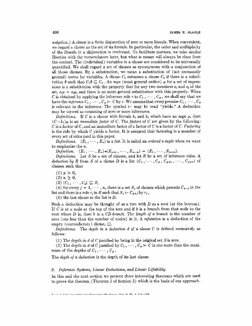
498 JAMES R. SLAGLE
seription.) A clause is a finite disjunction of zero or more literals. When convenient, we regard a clause as the set of its literals. In particular, the order and multiplicity of the liter~ls in a disjunction is irrelevant. To facilitate matters , we take similar liberties with the nomenclature later, but what is meant will always be clear from the context. The (individual) variables in a clause are considered to be universally quantified. We shall regard a set of clauses as synonymous with a conjunction of all those clauses. By a substitution, we mean a substi tution of (not necessarily ground) terms for variables. A clause C1 subsumes a clause C~ if there is a substi- tution 0 such tha t C10 ~ C2 • An mgu (most general unifier) t~ for a set of expres- sions is a substi tution with the proper ty tha t for any two members el and e2 of the set, el~ = e~, and there is no more general substi tut ion with this property. When C is obtained by applying the inference rule r to C~, • • • , C~, we shall say tha t we have the inference C~, , . • , Cp ~ C by r. We assume tha t every premise C~, • • • , Cp is relevant in the inference. The symbol F- may be read "yields." A deduction may be viewed as consisting of zero or more inferences.
Definitions. I f C is a clause with literals k~ and ks which have an mgu #, then ( C - k l ) t ~ is an immediate factor of C. The factors of C are given by the following: C is a factor of C, and an immediate factor of a factor of C is a factor of C. Factoring is the rule by which C yields a factor. I t is assumed tha t factoring is a member of every set of rules used in this paper.
Definitions. ( E l , • • • , E~) is a list. I t is called an ordered n-tuple when we want to emphasize the n.
Definition. ( E l , . . " , E,~)*(En+i , . . . , En+,~) = ( E l , . . . , En+~). Definitions. Let S be a set of clauses, and let R be a set of inference rules. A
deduction by R from S of a clause D is a list (C1, . . . , Cp, Cp+l, . . . , Cp+.) of clauses such tha t
(1) p > 0, (2) n >_ o, (3) { C 1 , . . . , C p } ~ S, (4) for every j = 1, • • • , n, there is a set Sj of clauses which precede Cp+j in the
list and there is a rule rj in R such tha t S~ ~- Cp+~ by r~, (5) the last clause in the list is D.
Such a deduction may be thought of as a tree with D as a root (at the bo t tom) . I f C is at a node at the top of the tree and if b is a branch from tha t node to the root where D is, then b is a CD-branch. The length of a branch is the number of arcs (one less than the number of nodes) in it. A refutation is a deduction of the empty (contradictory) clause, [].
Definitions. The depth in a deduction d of a clause C is defined recursively as follows:
(1) The depth in d of C justified by being in the original set S is zero. (2) The depth in d of C justified by C~, • • • , C~ t- C is one more than the maxi-
m u m of the depths of C~, . . . , Cp.
The depth of a deduction is the depth of its last clause.
3. Inference Systems, Linear Deductions, and Linear Liftability
In this and the next section we present three interesting theorems which are used to prove the theorem (Theorem 5 of Section 5) which is the basis of our approach.
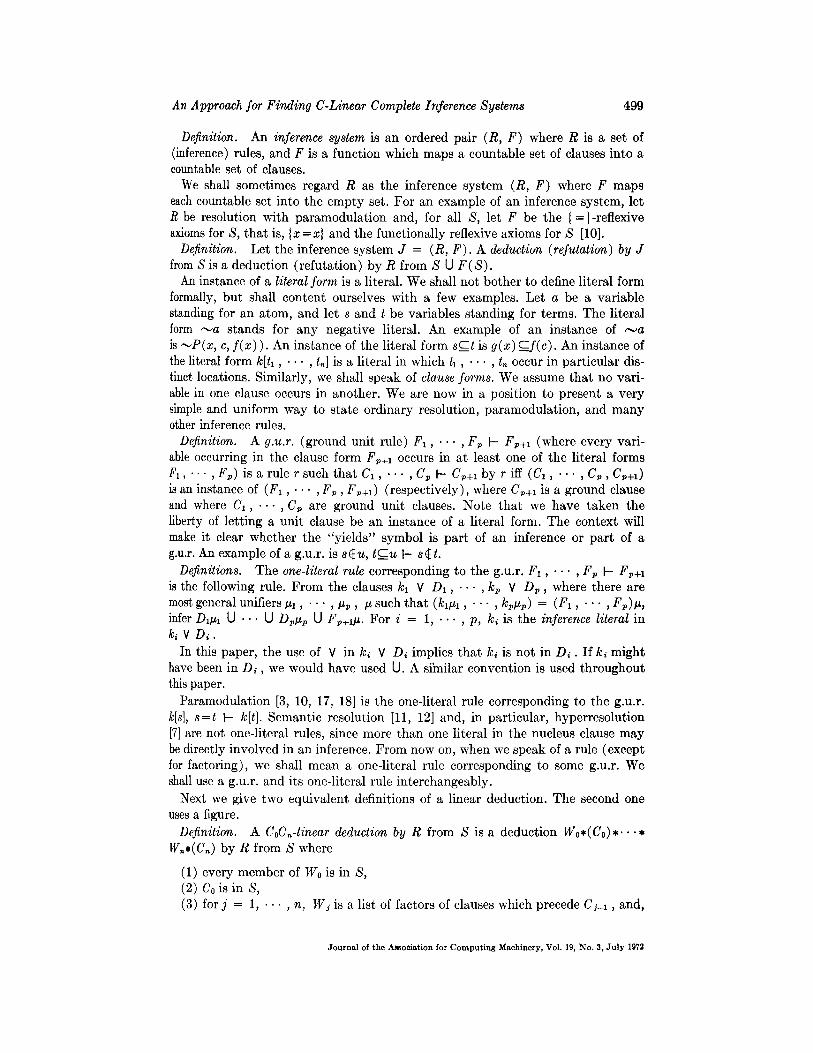
An Approach for Finding C-Linear Complete Inference Systems 499
Definitian. An inference system is an ordered pair (R, F) where R is a set of (inference) rules, and F is a funct ion which maps a countable set of clauses into a countable set of clauses.
We shall sometimes regard R as the inference sys tem (R, F ) where F maps each countable set into the e m p t y set. For an example of an inference system, let R be resolution with pa ramodula t ion and, for all S, let F be the {= }-reflexive axioms for S, t ha t is, Ix =x} and the funct ional ly reflexive axioms for S [10].
Definition. Let the inference sys tem J = (R, F ) . A deduction (refutation) by J from S is a deduct ion ( refuta t ion) by R from S U F(S).
An instance of a literal form is a literal. We shall not bo ther to define literal form formally, bu t shall content ourselves with a few examples. Let a be a variable standing for an a tom, and let s and t be variables s tanding for terms. The literal form ~ a s tands for any negative literal. An example of an instance of H a is uP(x, c, f(x) ). An instance of the literal form se t is g(x) Cf(c). An instance of the literal form k[tl, • • • , tn] is a literal in which t l , • • • , tn occur in par t icular dis- tinct locations. Similarly, we shall speak of clause forms. We assume tha t no vari- able in one clause occurs in another . We are now in a posit ion to present a very simple and uniform way to s tate ord inary resolution, paramodula t ion , and m a n y other inference rules.
Definition. A g.u.r. (ground uni t rule) F1, . . - , Fp b- Fp+l (where every vari- able occurring in the clause form Fp+~ occurs in at least one of the literal forms El, . . . , Fp) is a rule r such t h a t C1, - - . , C~ b- Cp+l by r iff (C1, " " , Cp, Cp+l) is an instance of (F1, . . . , Fp , Fp+l) ( respect ively) , where Cp+l is a ground clause and where C1, . - - , Cp are g round unit clauses. Note t h a t we have t aken the liberty of let t ing a uni t clause be an instance of a literal form. The context will make it clear whether the "y ie lds" symbol is pa r t of an inference or pa r t of a g.u.r. An example of a g.u.r, is s~u, t~u t- set.
Definitions. T he one-literal rule corresponding to the g.u.r. F1, . . . , Fp t- F~+i is the following rule. F r o m the clauses k~ V D1, • • • , kp V D p , where there are most general unifiers #1, • • • , tip, # such t h a t (k~/ul, • • • , k p ~ ) = (F~, • • • , F~)#, infer D ~ i U . . . [J Dpt~p U Fp+ltt. Fo r i = 1, . . . , p, k~ is the inference literal in k~ Y D i .
In this paper, the use of V in k~ Y D~ implies t ha t k~ is not in D~. I f k~ migh t have been in D~, we would have used tJ. A similar convent ion is used t h roughou t this paper.
Paramodula t ion [3, 10, 17, 18] is the one-literal rule corresponding to the g.u.r. k[s], s=t ~- k[t]. Semant ic resolution [11, 12] and, in part icular , hyperresolut ion [7] are not one-literal rules, since more than one literal in the nucleus clause m a y be directly involved in an inference. F r o m now on, when we speak of a rule (except for factoring), we shall mean a one-literal rule corresponding to some g.u.r. We shall use a g.u.r, and its one-literal rule in terchangeably.
Next we give two equivalent definitions of a linear deduct ion. The second one uses a figure.
Definition. A CoCn-linear deduction by R from S is a deduct ion W0*(C0)* . . . * W~*(C,) by R f rom S where
(1) every member of W0 is in S, (2) Co is in S, (3) for j = 1, . - . , n, Wi is a list of factors of clauses which precede C~._1, and,
Journal of the Association for Computing Machinery, Vol. 19, No. 3, July 1972
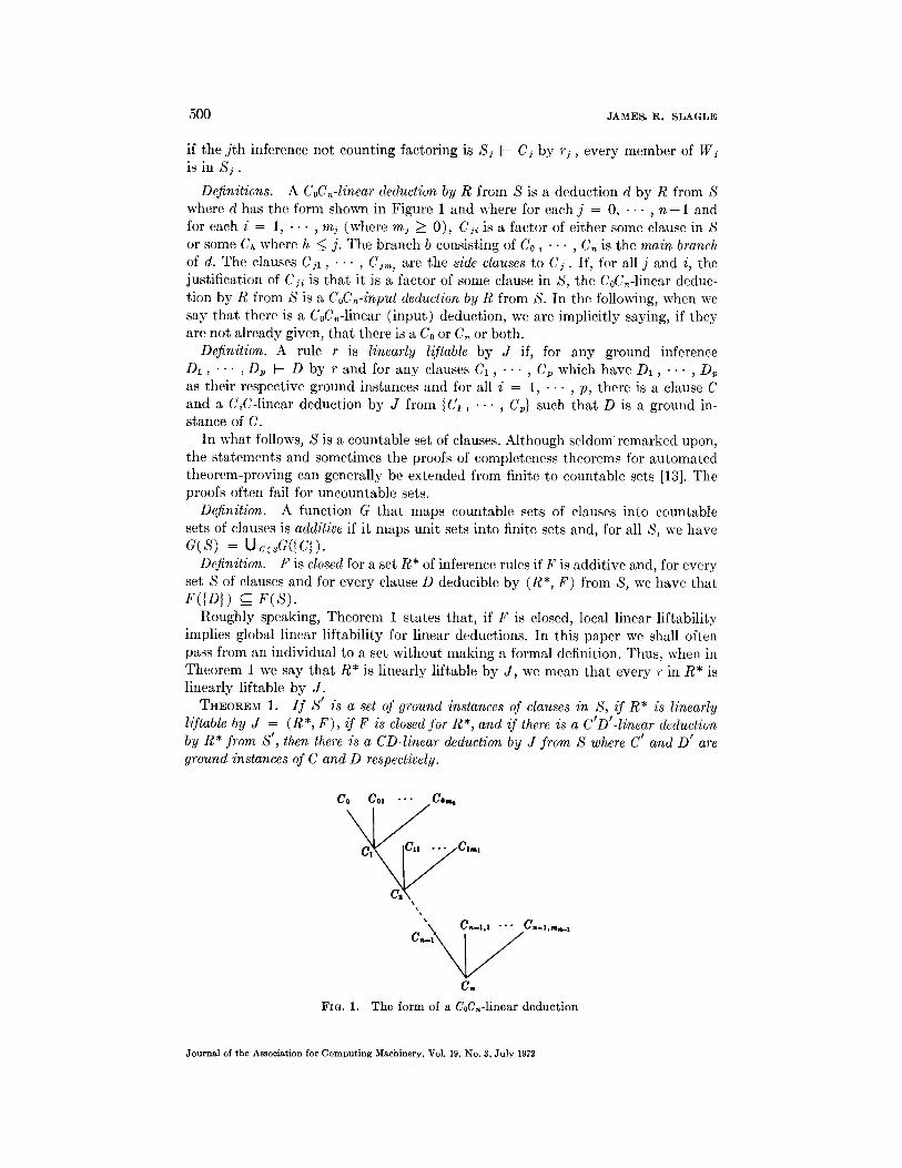
5 0 0 JAMES. R . S L A G L E
if the j th inference not counting factoring is Sj ~- Ci by r j , every member of Wj is in S j .
Definitions. A CoCn-linear deduction by R from S is a deduction d by R from S where d has the form shown in Figure 1 and where for each j = 0, • • • , n - 1 and for each i = 1, . . . , mi (where mi >_ 0), Cj.i is a factor of either some clause in S or some CA where h < j. The branch b consisting of Co, "-" , Cn is the main branch of d. The clauses C jl , • • • , C~mj are the side clauses to C~. If, for all j and i, the justification of Cil is tha t it is a factor of some clause in S, the CoC~-linear deduc- tion by R from S is a CoC,~-input deduction by R from S. In the following, when we say tha t there is a CoCn-linear ( input) deduction, we are implicitly saying, if they are not already given, that there is a Co or Cn or both.
Definition. A rule r is linearly liftable by J if, for any ground inference D i , ' " ,Dp ~- D b y r a n d for any c l a u s e s C 1 , . . . , C p w h i c h h a v e D ~ , . . . , D p as their respective ground instances and for all i = 1, . . . , p, there is a clause C and a CiC-linear deduction by J from {C~, . . . , Cp} such tha t D is a ground in- stance of C.
In what follows, S is a countable set of clauses. Although seldom remarked upon, the s tatements and sometimes the proofs of completeness theorems for automated theorem-proving can generally be extended from finite to countable sets [13]. The proofs often fail for uncountable sets.
Definition. A function G tha t maps countable sets of clauses into countable sets of clauses is additive if it maps unit sets into finite sets and, for all S, we have G(S) = Uc~G({C}) .
Definition. F is closed for a set R* of inference rules if F is additive and, for every set S of clauses and for every clause D deducible by (R*, F) from S, we have that F({D}) _c F(S) .
Roughly speaking, Theorem 1 states that , if F is closed, local linear liftability implies global linear liftability for linear deductions. In this paper we shall often pass from an individual to a set without making a formal definition. Thus, when in Theorem 1 we say tha t R* is linearly liftable by J , we mean tha t every r in R* is linearly liftable by J .
THEOREM 1. I f S' is a set of ground instances of clauses in S, if R* is linearly liftable by J = (R*, F), if F is closed for R*, and if there is a C'D'-linear deduction by R* from S', then there is a CD-linear deduction by J from S where C' and D' are ground instances of C and D respectively.
Co Col "" C o t • C1.1
x
x \ ~ n - - l , l " " " ~n- - l ,m~_l
C .
FiG. 1. The form of a CoCn-linear deduction
Journal of the Assoc ia t ion for C o m p u t i n g Machinery . Yol. 19. No. 3. Ju ly 1972
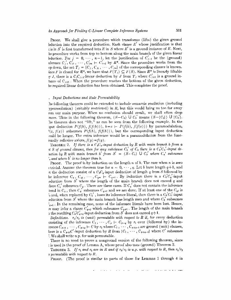
An Approach for Finding C-Linear Complete Inference Systems 501
PROOF. We shall give a procedure which transforms (lifts) the given ground [eduction into the required deduction. Each clause E ! whose justification is tha t t is in S t is first t ransformed into E in S where E ! is a ground instance of E: Next, he procedure works from top to bo t tom along the main branch of the given linear [eduction. For j = 0, . . . , n - l , let the justification of C~+1 be the (ground) nference C j , C~1, " " , C~m t-- C~+1 by R*. Since the procedure works from the 0p down, the set Tj = {Cj, C n , " ' " , C~} of the corresponding clauses is known. linee F is closed for R*, we have tha t F(T~) ~ F(S) . Since R* is linearly liftable ,y J, there is a CjCj+~-linear deduction by J from Ti where C~+~ is a ground in- tance of Cj+~. When the procedure reaches the bo t tom of the given deduction, he required linear deduction has been obtained. This completes the proof.
Input Deductions and Rule Permutability
:he following theorem could be extended to include semantic resolution (including yperresolution) (suitably restricted) in R, but this would bring us too far away tom our main purpose. When no confusion should result, we shall often drop ,races. Thus in the following theorem, (S--Co) U Co' means ( S - I C 0 } ) U {C0'}. 'he theorem does not " l i f t ," as can be seen from the following example. In the 1put deduction P(f(b), f( f(b) ) ), b=c t- P(f(b), f( f(c) ) ) by paramodulat ion, )(x, f (x)) subsumes P(f(b), f ( f (b))) , but the corresponding input deduction :ould be longer. The extra inference would be a paramodulat ion from the func- [onally reflexive axiom, f(y) = f ( y ) . THEOREM 2. I f there is a CoCn-input deduction by R with main branch b from a
~t S of ground clauses, then for any subclause Co' of Co there is a Co'Cn'-input de- uction by R with main branch b' from S' = (S-Co) U Co' where Cn' subsumes !~ and where b' is no longer than b.
PROOF. The proof is by induction on the length n of b. The case when n is zero trivial. Assume the theorem true for n = 0, • • • , q. Let b have length q + l , and
~t the deduction consist of a CoCq-input deduction of length q from S followed by he inference Cq, Cql, " " , Cqm ~- Cq+l. By induction there is a Co'Cq'-input eduction from S' where the length of the main branch does not exceed q and :here Cq' subsumes Cq. There are three cases. If Cq' does not contain the inference feral in Cq, then Cq' subsumes Cq+l and we are done. If at least one of the Cq~ is ~0 and, when replaced by Co' , loses its inference literal, then there is a C0'Co'-input eduction from S' where the main branch has length zero and where Co' subsumes !q+~. In the remaining case, none of the inference literals have been lost. Hence,
!
~e may infer a clause Cq+~ which subsumes Cq+~. The length of the main branch the resulting Co!C!q+~-input deduction from S' does not exceed q + 1. Definitions. r~/~ is (unit) permutable with respect to R if, for every deduction
onsisting of the inference C1, . " , Cp ~ Cp+q by rl over (followed by) the in- ~rence Cp+l, • • • , Cp+q ~ C by r2 where C~, • • • , Cp+q-1 are ground (unit) clauses, here is a Cp+~C'-input deduction by R from {C~, . . . , Cp+q_~} where C' subsumes !. We shall write u.p. for unit permutable.
There is no need to prove a nonground version of the following theorem, since l is used in the proof of Lemma A, whose proof also uses (ground) Theorem 2.
THEOREM 3. I f r~ and r2 are in R and if rl/re is u.p. with respect to R, then rJr2 s permutable with respect to R.
PROOF. (The proof is similar to parts of those for Lemmas 1 through 4 in