PRODUCT USER MANUAL For Global Physical Analysis …cmems-resources.cls.fr/documents/PUM/CMEMS-GLO-PUM-001-015.pdf · For Global Physical Analysis and Coupled System Forecasting Product

PRODUCT USER MANUAL

For Global Physical Analysis and Coupled System Forecasting Product

GLOBAL_ANALYSIS_FORECAST_PHYS_001_015

Issue: 2.5

Contributors: C. Harris, E. Blockley, M. Price

CMEMS version scope : V3.1

Approval Date : 11/07/2017

PUM for Global Physical Analysis and Coupled System Forecasting Product

GLO_ANALYSIS_FORECAST_PHYS_001_015

Ref: CMEMS-GLO-PUM-001-015

Date : 3 Jul 2017

Issue : 2.5

© EU Copernicus Marine Service– Public Page 2/ 21

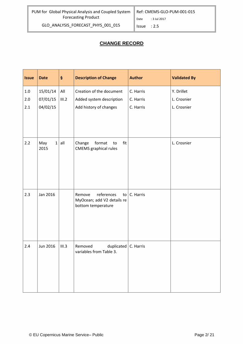
CHANGE RECORD

Issue Date § Description of Change Author Validated By

1.0

2.0

2.1

15/01/14

07/01/15

04/02/15

All

III.2

Creation of the document

Added system description

Add history of changes

C. Harris

C. Harris

C. Harris

Y. Drillet

L. Crosnier

L. Crosnier

2.2 May 1 2015

all Change format to fit CMEMS graphical rules

L. Crosnier

2.3 Jan 2016 Remove references to MyOcean; add V2 details re bottom temperature

C. Harris

2.4 Jun 2016 III.3 Removed duplicated variables from Table 3.

C. Harris




Date : 3 Jul 2017

Issue : 2.5


2.5 Jul 2017 All Updated for V3.1 C. Harris, M. Price, C. Derval




Date : 3 Jul 2017

Issue : 2.5


TABLE OF CONTENTS

I INTRODUCTION ......................................................................................................................................... 6

I.1 Summary ...................................................................................................................................................... 6

I.2 History of changes ....................................................................................................................................... 6

II DESCRIPTION OF THE PRODUCT SPECIFICATION .......................................................................... 7

II.1 General Information .................................................................................................................................. 7

II.2 Details of datasets ...................................................................................................................................... 8

II.3 Production System description ............................................................................................................... 10

II.4 Processing information ............................................................................................................. 16

II.4.1 Update Time .................................................................................................................................... 16

II.4.2 Temporal extend of analysis and forecast stored on delivery mechanism (if relevant) ................... 16

III HOW TO DOWNLOAD A PRODUCT .................................................................................................. 17

III.1 Download a product through the CMEMS Web Portal Subsetter Service ....................................... 17

III.2 Download a product through the CMEMS FTP Service .................................................................... 17

III.3 Download a product through the CMEMS DGF (DirectGetFile) Service ........................................ 17

IV Files NOMENCLATURE and Format ....................................................................................................... 18

IV.1 Nomenclature of files when downloaded through the CMEMS Web Portal Subsetter Service ...... 18

IV.2 Nomenclature of files when downloaded through the CMEMS FTP Service ................................... 18

IV.3 Nomenclature of files when downloaded through the CMEMS DGF Service .................................. 19

IV.4 Structure and semantic of NetCDF maps files ..................................................................................... 20

IV.5 Other information: mean centre of Products, land mask value, missing value ................................ 21

IV.6 Reading software .................................................................................................................................... 21




Date : 3 Jul 2017

Issue : 2.5


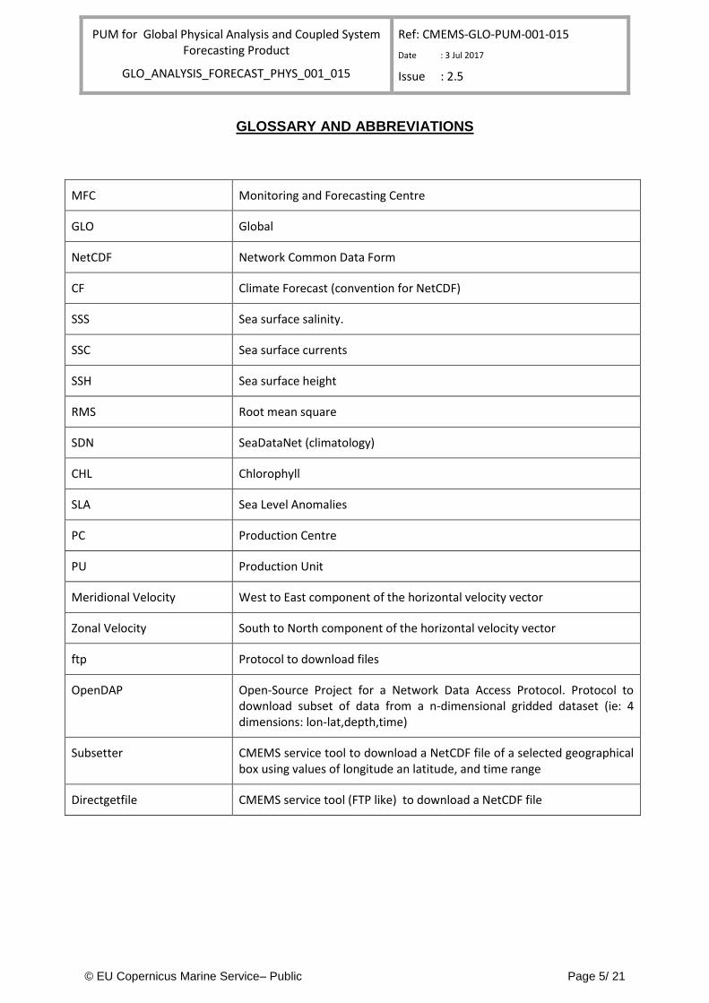
GLOSSARY AND ABBREVIATIONS

MFC Monitoring and Forecasting Centre

GLO Global

NetCDF Network Common Data Form

CF Climate Forecast (convention for NetCDF)

SSS Sea surface salinity.

SSC Sea surface currents

SSH Sea surface height

RMS Root mean square

SDN SeaDataNet (climatology)

CHL Chlorophyll

SLA Sea Level Anomalies

PC Production Centre

PU Production Unit

Meridional Velocity West to East component of the horizontal velocity vector

Zonal Velocity South to North component of the horizontal velocity vector

ftp Protocol to download files

OpenDAP Open-Source Project for a Network Data Access Protocol. Protocol to download subset of data from a n-dimensional gridded dataset (ie: 4 dimensions: lon-lat,depth,time)

Subsetter CMEMS service tool to download a NetCDF file of a selected geographical box using values of longitude an latitude, and time range

Directgetfile CMEMS service tool (FTP like) to download a NetCDF file




Date : 3 Jul 2017

Issue : 2.4


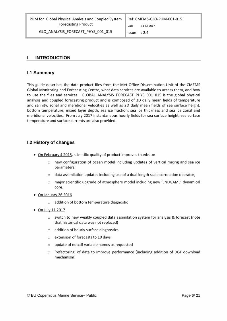
I INTRODUCTION

I.1 Summary

This guide describes the data product files from the Met Office Dissemination Unit of the CMEMS Global Monitoring and Forecasting Centre, what data services are available to access them, and how to use the files and services. GLOBAL_ANALYSIS_FORECAST_PHYS_001_015 is the global physical analysis and coupled forecasting product and is composed of 3D daily mean fields of temperature and salinity, zonal and meridional velocities as well as 2D daily mean fields of sea surface height, bottom temperature, mixed layer depth, sea ice fraction, sea ice thickness and sea ice zonal and meridional velocities. From July 2017 instantaneous hourly fields for sea surface height, sea surface temperature and surface currents are also provided.

I.2 History of changes

On February 4 2015, scientific quality of product improves thanks to:

o new configuration of ocean model including updates of vertical mixing and sea ice parameters,

o data assimilation updates including use of a dual length scale correlation operator,

o major scientific upgrade of atmosphere model including new ‘ENDGAME’ dynamical core.

On January 26 2016

o addition of bottom temperature diagnostic

On July 11 2017

o switch to new weakly coupled data assimilation system for analysis & forecast (note that historical data was not replaced)

o addition of hourly surface diagnostics

o extension of forecasts to 10 days

o update of netcdf variable names as requested

o ‘refactoring’ of data to improve performance (including addition of DGF download mechanism)




Date : 3 Jul 2017

Issue : 2.5


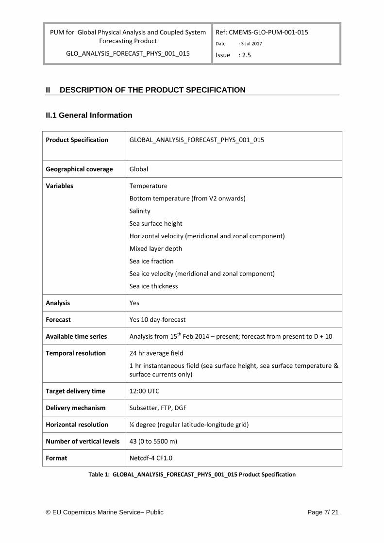
II DESCRIPTION OF THE PRODUCT SPECIFICATION

II.1 General Information

Product Specification GLOBAL_ANALYSIS_FORECAST_PHYS_001_015

Geographical coverage Global

Variables Temperature

Bottom temperature (from V2 onwards)

Salinity

Sea surface height

Horizontal velocity (meridional and zonal component)

Mixed layer depth

Sea ice fraction

Sea ice velocity (meridional and zonal component)

Sea ice thickness

Analysis Yes

Forecast Yes 10 day-forecast

Available time series Analysis from 15th Feb 2014 – present; forecast from present to D + 10

Temporal resolution 24 hr average field

1 hr instantaneous field (sea surface height, sea surface temperature & surface currents only)

Target delivery time 12:00 UTC

Delivery mechanism Subsetter, FTP, DGF

Horizontal resolution ¼ degree (regular latitude-longitude grid)

Number of vertical levels 43 (0 to 5500 m)

Format Netcdf-4 CF1.0

Table 1: GLOBAL_ANALYSIS_FORECAST_PHYS_001_015 Product Specification




Date : 3 Jul 2017

Issue : 2.5


Detailed information on the systems and products are on CMEMS web site: http://marine.copernicus.eu.

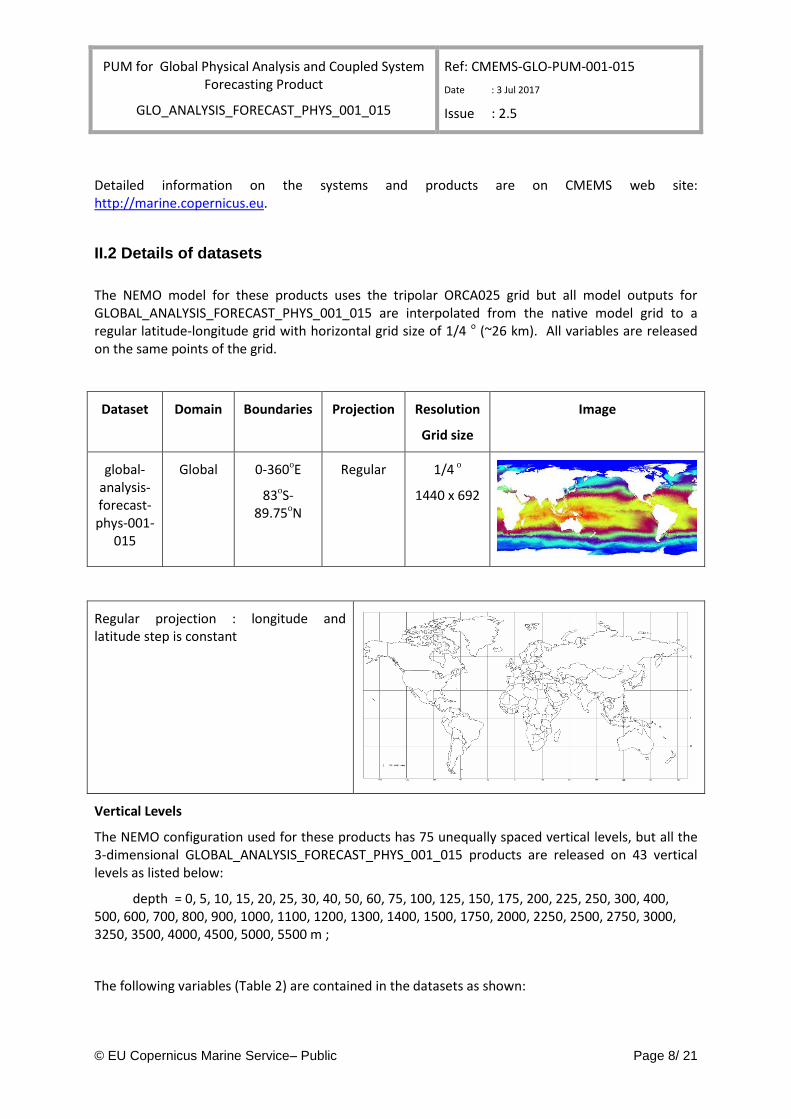
II.2 Details of datasets

The NEMO model for these products uses the tripolar ORCA025 grid but all model outputs for GLOBAL_ANALYSIS_FORECAST_PHYS_001_015 are interpolated from the native model grid to a regular latitude-longitude grid with horizontal grid size of 1/4 o (~26 km). All variables are released on the same points of the grid.

Dataset Domain Boundaries Projection Resolution

Grid size

Image

global-analysis-forecast-phys-001-

015

Global 0-360oE

83oS-89.75oN

Regular 1/4 o

1440 x 692

Regular projection : longitude and latitude step is constant

Vertical Levels

The NEMO configuration used for these products has 75 unequally spaced vertical levels, but all the 3-dimensional GLOBAL_ANALYSIS_FORECAST_PHYS_001_015 products are released on 43 vertical levels as listed below:

depth = 0, 5, 10, 15, 20, 25, 30, 40, 50, 60, 75, 100, 125, 150, 175, 200, 225, 250, 300, 400, 500, 600, 700, 800, 900, 1000, 1100, 1200, 1300, 1400, 1500, 1750, 2000, 2250, 2500, 2750, 3000, 3250, 3500, 4000, 4500, 5000, 5500 m ;

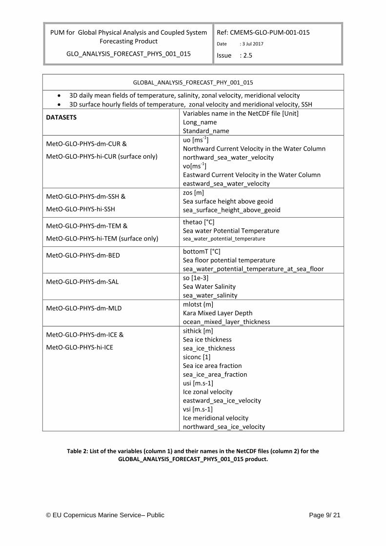
The following variables (Table 2) are contained in the datasets as shown:

http://marine.copernicus.eu/




Date : 3 Jul 2017

Issue : 2.5


GLOBAL_ANALYSIS_FORECAST_PHY_001_015

3D daily mean fields of temperature, salinity, zonal velocity, meridional velocity

3D surface hourly fields of temperature, zonal velocity and meridional velocity, SSH

DATASETS Variables name in the NetCDF file [Unit] Long_name Standard_name

MetO-GLO-PHYS-dm-CUR &

MetO-GLO-PHYS-hi-CUR (surface only)

uo [ms-1] Northward Current Velocity in the Water Column northward_sea_water_velocity vo[ms-1] Eastward Current Velocity in the Water Column eastward_sea_water_velocity

MetO-GLO-PHYS-dm-SSH &

MetO-GLO-PHYS-hi-SSH

zos [m] Sea surface height above geoid sea_surface_height_above_geoid

MetO-GLO-PHYS-dm-TEM &

MetO-GLO-PHYS-hi-TEM (surface only)

thetao [°C] Sea water Potential Temperature sea_water_potential_temperature

MetO-GLO-PHYS-dm-BED bottomT [°C] Sea floor potential temperature sea_water_potential_temperature_at_sea_floor

MetO-GLO-PHYS-dm-SAL so [1e-3] Sea Water Salinity sea_water_salinity

MetO-GLO-PHYS-dm-MLD mlotst (m] Kara Mixed Layer Depth ocean_mixed_layer_thickness

MetO-GLO-PHYS-dm-ICE &

MetO-GLO-PHYS-hi-ICE

sithick [m] Sea ice thickness sea_ice_thickness siconc [1] Sea ice area fraction sea_ice_area_fraction usi [m.s-1] Ice zonal velocity eastward_sea_ice_velocity vsi [m.s-1] Ice meridional velocity northward_sea_ice_velocity

Table 2: List of the variables (column 1) and their names in the NetCDF files (column 2) for the GLOBAL_ANALYSIS_FORECAST_PHYS_001_015 product.




Date : 3 Jul 2017

Issue : 2.5


II.3 Production System description

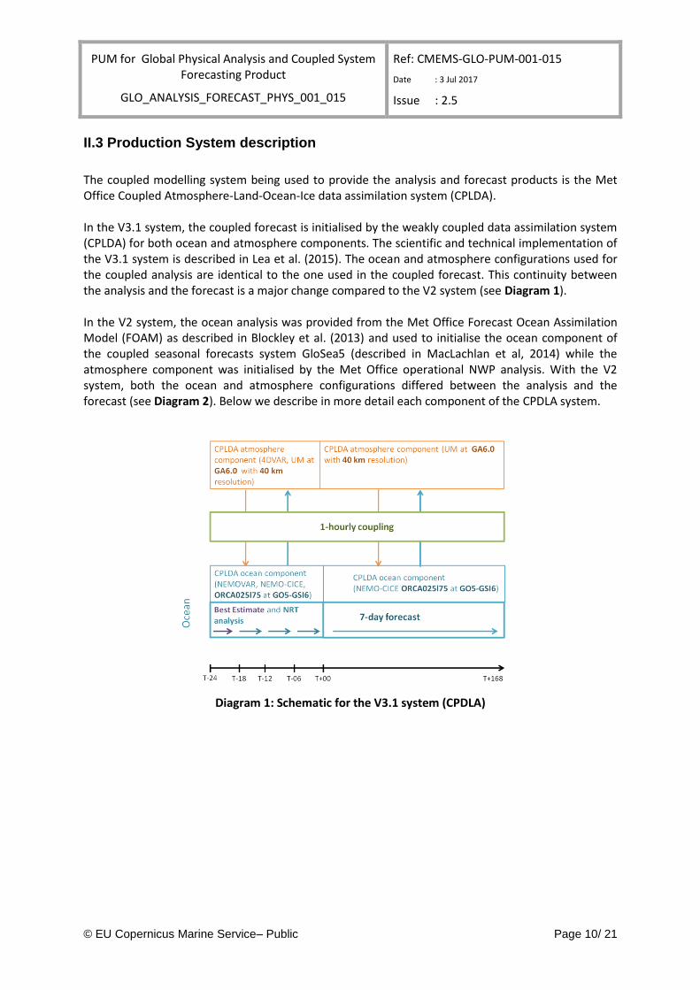
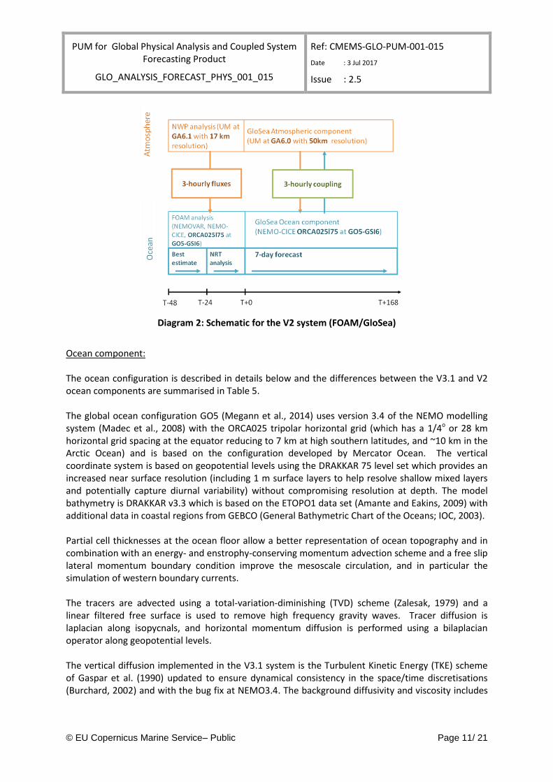
The coupled modelling system being used to provide the analysis and forecast products is the Met Office Coupled Atmosphere-Land-Ocean-Ice data assimilation system (CPLDA). In the V3.1 system, the coupled forecast is initialised by the weakly coupled data assimilation system (CPLDA) for both ocean and atmosphere components. The scientific and technical implementation of the V3.1 system is described in Lea et al. (2015). The ocean and atmosphere configurations used for the coupled analysis are identical to the one used in the coupled forecast. This continuity between the analysis and the forecast is a major change compared to the V2 system (see Diagram 1). In the V2 system, the ocean analysis was provided from the Met Office Forecast Ocean Assimilation Model (FOAM) as described in Blockley et al. (2013) and used to initialise the ocean component of the coupled seasonal forecasts system GloSea5 (described in MacLachlan et al, 2014) while the atmosphere component was initialised by the Met Office operational NWP analysis. With the V2 system, both the ocean and atmosphere configurations differed between the analysis and the forecast (see Diagram 2). Below we describe in more detail each component of the CPDLA system.

Diagram 1: Schematic for the V3.1 system (CPDLA)




Date : 3 Jul 2017

Issue : 2.5


Diagram 2: Schematic for the V2 system (FOAM/GloSea)

Ocean component: The ocean configuration is described in details below and the differences between the V3.1 and V2 ocean components are summarised in Table 5. The global ocean configuration GO5 (Megann et al., 2014) uses version 3.4 of the NEMO modelling system (Madec et al., 2008) with the ORCA025 tripolar horizontal grid (which has a 1/4o or 28 km horizontal grid spacing at the equator reducing to 7 km at high southern latitudes, and ~10 km in the Arctic Ocean) and is based on the configuration developed by Mercator Ocean. The vertical coordinate system is based on geopotential levels using the DRAKKAR 75 level set which provides an increased near surface resolution (including 1 m surface layers to help resolve shallow mixed layers and potentially capture diurnal variability) without compromising resolution at depth. The model bathymetry is DRAKKAR v3.3 which is based on the ETOPO1 data set (Amante and Eakins, 2009) with additional data in coastal regions from GEBCO (General Bathymetric Chart of the Oceans; IOC, 2003). Partial cell thicknesses at the ocean floor allow a better representation of ocean topography and in combination with an energy- and enstrophy-conserving momentum advection scheme and a free slip lateral momentum boundary condition improve the mesoscale circulation, and in particular the simulation of western boundary currents. The tracers are advected using a total-variation-diminishing (TVD) scheme (Zalesak, 1979) and a linear filtered free surface is used to remove high frequency gravity waves. Tracer diffusion is laplacian along isopycnals, and horizontal momentum diffusion is performed using a bilaplacian operator along geopotential levels. The vertical diffusion implemented in the V3.1 system is the Turbulent Kinetic Energy (TKE) scheme of Gaspar et al. (1990) updated to ensure dynamical consistency in the space/time discretisations (Burchard, 2002) and with the bug fix at NEMO3.4. The background diffusivity and viscosity includes




Date : 3 Jul 2017

Issue : 2.5


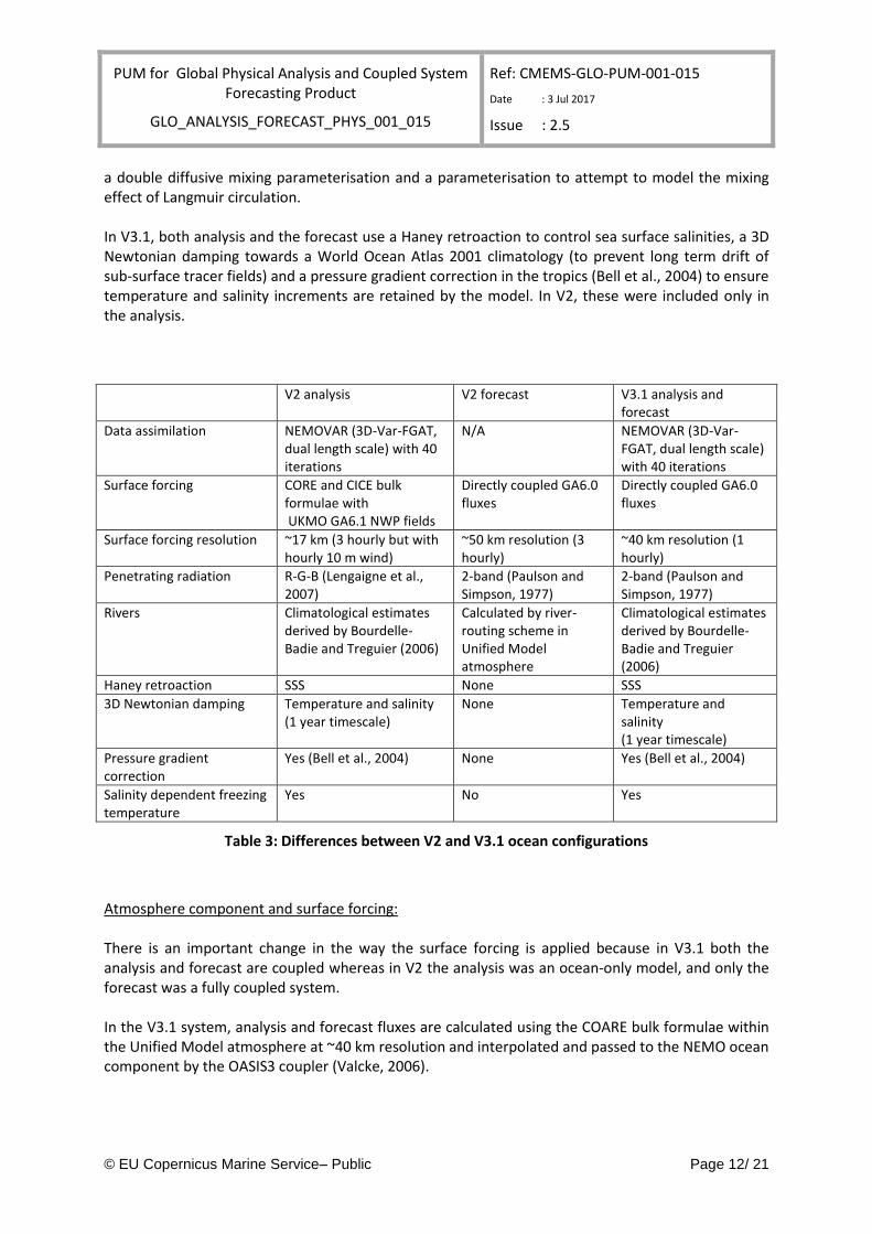
a double diffusive mixing parameterisation and a parameterisation to attempt to model the mixing effect of Langmuir circulation. In V3.1, both analysis and the forecast use a Haney retroaction to control sea surface salinities, a 3D Newtonian damping towards a World Ocean Atlas 2001 climatology (to prevent long term drift of sub-surface tracer fields) and a pressure gradient correction in the tropics (Bell et al., 2004) to ensure temperature and salinity increments are retained by the model. In V2, these were included only in the analysis. V2 analysis V2 forecast V3.1 analysis and

forecast

Data assimilation NEMOVAR (3D-Var-FGAT, dual length scale) with 40 iterations

N/A NEMOVAR (3D-Var-FGAT, dual length scale) with 40 iterations

Surface forcing CORE and CICE bulk formulae with UKMO GA6.1 NWP fields

Directly coupled GA6.0 fluxes

Directly coupled GA6.0 fluxes

Surface forcing resolution ~17 km (3 hourly but with hourly 10 m wind)

~50 km resolution (3 hourly)

~40 km resolution (1 hourly)

Penetrating radiation R-G-B (Lengaigne et al., 2007)

2-band (Paulson and Simpson, 1977)

2-band (Paulson and Simpson, 1977)

Rivers Climatological estimates derived by Bourdelle-Badie and Treguier (2006)

Calculated by river-routing scheme in Unified Model atmosphere

Climatological estimates derived by Bourdelle-Badie and Treguier (2006)

Haney retroaction SSS None SSS

3D Newtonian damping Temperature and salinity (1 year timescale)

None Temperature and salinity (1 year timescale)

Pressure gradient correction

Yes (Bell et al., 2004) None Yes (Bell et al., 2004)

Salinity dependent freezing temperature

Yes No Yes

Table 3: Differences between V2 and V3.1 ocean configurations

Atmosphere component and surface forcing: There is an important change in the way the surface forcing is applied because in V3.1 both the analysis and forecast are coupled whereas in V2 the analysis was an ocean-only model, and only the forecast was a fully coupled system. In the V3.1 system, analysis and forecast fluxes are calculated using the COARE bulk formulae within the Unified Model atmosphere at ~40 km resolution and interpolated and passed to the NEMO ocean component by the OASIS3 coupler (Valcke, 2006).




Date : 3 Jul 2017

Issue : 2.5


In the V2 system, the forecast fluxes were similar to the V3.1 system but the analysis used interpolated atmosphere fields from the operational Met Office global NWP configuration of the Unified Model (currently at ~17 km resolution) and uses CORE bulk formulae (Large and Yeager, 2004) to calculate the turbulent fluxes. The V3.1 atmospheric component is the GA6.0 atmosphere configuration for both the analysis and forecast while V2 was using GA6.0 for the analysis and GA6.1 for the forecast (note that this distinction largely relates to aspects of the land-surface treatment and is probably largely irrelevant from the ocean point of view). The V3.1 atmosphere data assimilation system is described in details in Lea et al. (2015). It uses an incremental strong constraint 4DVAR system similar to Rawlins et al (2007). One addition to the system described in Lea et al. (2015) is that the V3.1 atmosphere data assimilation uses a variational bias correction (VarBC) to continuously update the bias correction applied to observations. Sea ice component: The sea ice model (CICE version 4.1; Hunke and Lipscomb, 2010) runs on the same ORCA025 grid as NEMO, and with 5 thickness categories. The CICE model determines the spatial and temporal evolution of the ice thickness distribution (ITD) due to advection, thermodynamic growth and melt, and mechanical redistribution / ridging (Thorndike et al., 1975). Due to constraints when running coupled to the Unified Model atmosphere, the V3.1 system uses the zero-layer thermodynamic model of Semtner (1976), with a single layer of both ice and snow. Ice dynamics are calculated using the elastic-viscous-plastic (EVP) scheme of Hunke and Dukowicz (2002). In V3.1, for both the analysis and forecast, the ice top and bottom conductive heat fluxes are calculated within the atmosphere model, interpolated by OASIS, and then passed to NEMO from where they can be accessed by CICE. In the V2 forecast, the heat fluxes calculated by the atmosphere model were also used but in the V2 ocean-only analysis CICE used its own bulk formulation to specify surface boundary conditions. The freezing temperature for both V3.1 analysis and forecast is dependent on salinity to provide a more realistic representation of ice melting and freezing mechanisms and to give better consistency when assimilating both sea surface temperature and sea ice concentration. In the V2 system, for technical reason, the salinity dependent freezing temperature was used only in the analysis, while the V2 forecast used a fixed freezing temperature of -1.8 degrees C. The GSI6 global sea-ice configuration used in the V3.1 system is detailed in Rae et al. (2014).




Date : 3 Jul 2017

Issue : 2.5


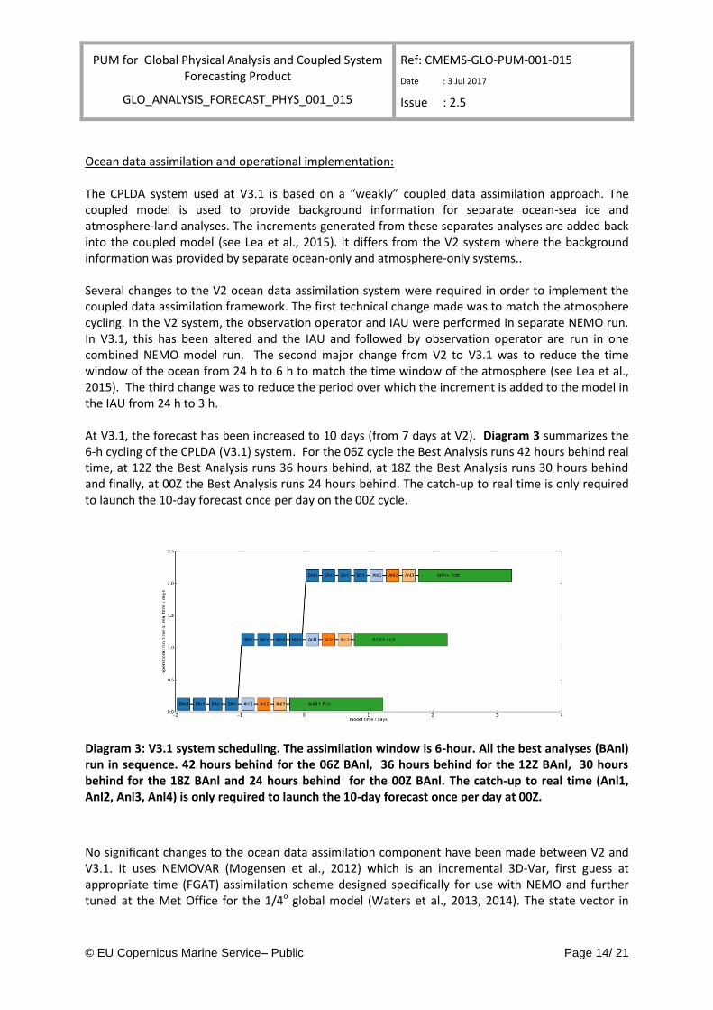
Ocean data assimilation and operational implementation: The CPLDA system used at V3.1 is based on a “weakly” coupled data assimilation approach. The coupled model is used to provide background information for separate ocean-sea ice and atmosphere-land analyses. The increments generated from these separates analyses are added back into the coupled model (see Lea et al., 2015). It differs from the V2 system where the background information was provided by separate ocean-only and atmosphere-only systems.. Several changes to the V2 ocean data assimilation system were required in order to implement the coupled data assimilation framework. The first technical change made was to match the atmosphere cycling. In the V2 system, the observation operator and IAU were performed in separate NEMO run. In V3.1, this has been altered and the IAU and followed by observation operator are run in one combined NEMO model run. The second major change from V2 to V3.1 was to reduce the time window of the ocean from 24 h to 6 h to match the time window of the atmosphere (see Lea et al., 2015). The third change was to reduce the period over which the increment is added to the model in the IAU from 24 h to 3 h. At V3.1, the forecast has been increased to 10 days (from 7 days at V2). Diagram 3 summarizes the 6-h cycling of the CPLDA (V3.1) system. For the 06Z cycle the Best Analysis runs 42 hours behind real time, at 12Z the Best Analysis runs 36 hours behind, at 18Z the Best Analysis runs 30 hours behind and finally, at 00Z the Best Analysis runs 24 hours behind. The catch-up to real time is only required to launch the 10-day forecast once per day on the 00Z cycle.

Diagram 3: V3.1 system scheduling. The assimilation window is 6-hour. All the best analyses (BAnl) run in sequence. 42 hours behind for the 06Z BAnl, 36 hours behind for the 12Z BAnl, 30 hours behind for the 18Z BAnl and 24 hours behind for the 00Z BAnl. The catch-up to real time (Anl1, Anl2, Anl3, Anl4) is only required to launch the 10-day forecast once per day at 00Z.

No significant changes to the ocean data assimilation component have been made between V2 and V3.1. It uses NEMOVAR (Mogensen et al., 2012) which is an incremental 3D-Var, first guess at appropriate time (FGAT) assimilation scheme designed specifically for use with NEMO and further tuned at the Met Office for the 1/4o global model (Waters et al., 2013, 2014). The state vector in




Date : 3 Jul 2017

Issue : 2.5


NEMOVAR consists of temperature, salinity, surface elevation, sea ice concentration and horizontal velocities. Key features of NEMOVAR are the multivariate relationships which are specified through a linearised balance operator (Weaver et al., 2005) and the use of an implicit diffusion operator to model background error correlations (Mirouze and Weaver, 2010). As detailed in Waters et al. (2013), the NEMOVAR system includes bias correction schemes for both SST and for altimeter data (using the CNES09 Mean Dynamic Topography of Rio et al., 2011 as a reference). The temperature and unbalanced salinity are assimilated using two horizontal correlation length scales (Mirouze et al., 2016) following the method described in Martin et al. (2007). The number of iterations is 40. No specific tuning has been made for the coupled system. Some future improvement could include recalculating the error covariances for a coupled model and for a 6-h window as well as tuning the altimeter bias correction. Observations assimilated are as follows:

Satellite SST data – sub-sampled level 2 Advanced Very High Resolution Radiometer (AVHRR) data from NOAA, MetOp, AMSR2, and Visible Infrared Imaging Radiometer Suite (VIIRS) satellites supplied by the Global High-Resolution Sea Surface Temperature (GHRSST) project.

In-situ SSTs – from moored buoys, drifting buoys and ships (these are considered unbiased and used as a reference for satellite SST bias correction)

Sea level anomaly observations – from Jason2, Jason3, CryoSat2, SARAL/AltiKa and Sentinel 3a (all from CMEMS product SEALEVEL_GLO_SLA_L3_NRT_OBSERVATIONS_008_044)

Sub-surface temperature and salinity profiles – from Argo profiling floats, underwater gliders, moored buoys, marine mammals, and manual profiling methods

Sea ice concentration - Special Sensor Microwave Imager/Sounder (SSMIS) data provided by the EUMETSAT Ocean Sea Ice Satellite Application Facility (OSI-SAF) as a daily gridded product on a 10km polar stereographic projection

Observations are read into NEMO and model fields are mapped into observation space using the NEMO observation operator to create model counterparts using bilinear interpolation in the horizontal and cubic splines in the vertical directions. Observations are assimilated using a 6 hour window (previously 24 h in V2) and constant increments are applied to the model over 3 hours in the incremental analysis update (IAU) step. Analysis updates are made to the state variables in the NEMO model with the exception of sea ice concentration updates which are made in the CICE model (updates increasing ice concentration are always made to the thinnest category ice, whilst updates decreasing ice concentration are made to the thinnest ice thickness category available in that grid cell).




Date : 3 Jul 2017

Issue : 2.5


II.4 Processing information

II.4.1 Update Time

GLOBAL_ANALYSIS_FORECAST_PHYS_001_015 products are updated daily at 12:00 UTC.

II.4.2 Temporal extend of analysis and forecast stored on delivery mechanism (if relevant)

Each day the (T-48h,T-24h] and (T-24h,T+00h] analyses are provided along with a 10 day forecast for all products (with the first day of the forecast being for the day of production). An archive of the (T-48h,T-24h] analyses will be retained indefinitely (as described in Table1 above).




Date : 3 Jul 2017

Issue : 2.5


III HOW TO DOWNLOAD A PRODUCT

III.1 Download a product through the CMEMS Web Portal Subsetter Service

You first need to register. Please find below the registration steps: http://marine.copernicus.eu/web/56-user-registration-form.php.

Once registered, the CMEMS FAQ http://marine.copernicus.eu/web/34-products-and-services-faq.php will guide you on How to download a product through the CMEMS Web Portal Subsetter Service.

III.2 Download a product through the CMEMS FTP Service


The ftp site is accessed using your CMEMS user name and password and the files are located in the directory called GLOBAL_ANALYSIS_FORECAST_PHYS_001_015.

III.3 Download a product through the CMEMS DGF (DirectGetFile) Service


Once registered, the CMEMS FAQ http://marine.copernicus.eu/web/34-products-and-services-faq.php will guide you on How to download a product through the CMEMS DGF Service.

http://marine.copernicus.eu/web/56-user-registration-form.php

http://marine.copernicus.eu/web/34-products-and-services-faq.php









Date : 3 Jul 2017

Issue : 2.5


IV FILES NOMENCLATURE AND FORMAT

The nomenclature of the downloaded files differs on the basis of the chosen download mechanism Subsetter, CMEMS FTP or DirectGetFile service.

IV.1 Nomenclature of files when downloaded through the CMEMS Web Portal Subsetter Service

GLOBAL_ANALYSIS_FORECAST_PHYS_001_015 files nomenclature when downloaded through the CMEMS Web Portal Subsetter is based on product dataset name and a numerical reference related to the request date on the MIS.

The scheme is: datasetname-nnnnnnnnnnnnn.nc

where :

.datasetname is the METOFFICE-GLO-PHYS-FA-DAILY character string

. nnnnnnnnnnnnn: 13 digit integer corresponding to the current time (download time) in milliseconds since January 1, 1970 midnight UTC.

.nc: standard NetCDF filename extension.

Example: MetO-GLO-PHYS-dm-TEM-1303461772348.nc

IV.2 Nomenclature of files when downloaded through the CMEMS FTP Service

GLOBAL_ANALYSIS_PHYS_001_015 files nomenclature when downloaded through the CMEMS FTP service is based as follows:

{producer}_{config}_{model}_{region}_{parameter}_{bul date}_{freq flag}{average flag}{valid date}.nc

where

· producer is a short version of the CMEMS production unit i.e. metoffice.

· config identifies the producing system i.e. coupled.

· model identifies the model configuration i.e. orca025

· region is a three letter code for the region i.e. GL4

· parameter is a three letter code for the parameter or parameter (see Table 4).

· bul date bYYYYMMDD is the bulletin date the product was produced

· freq flag is the frequency of data values in the file (i.e. d = daily)

· average flag is i=instantaneous, m=mean (usually daily)

· valid date YYYYMMDD is the validity day of the data in the file




Date : 3 Jul 2017

Issue : 2.5


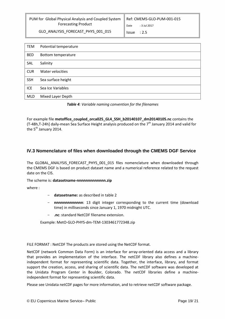
TEM Potential temperature

BED Bottom temperature

SAL Salinity

CUR Water velocities

SSH Sea surface height

ICE Sea Ice Variables

MLD Mixed Layer Depth

Table 4: Variable naming convention for the filenames

For example file metoffice_coupled_orca025_GL4_SSH_b20140107_dm20140105.nc contains the (T-48h,T-24h] daily-mean Sea Surface Height analysis produced on the 7th January 2014 and valid for the 5th January 2014.

IV.3 Nomenclature of files when downloaded through the CMEMS DGF Service

The GLOBAL_ANALYSIS_FORECAST_PHYS_001_015 files nomenclature when downloaded through the CMEMS DGF is based on product dataset name and a numerical reference related to the request date on the CIS.

The scheme is: datasetname-nnnnnnnnnnnnn.zip

where :

- datasetname: as described in table 2

- nnnnnnnnnnnnn: 13 digit integer corresponding to the current time (download time) in milliseconds since January 1, 1970 midnight UTC.

- .nc: standard NetCDF filename extension.

Example: MetO-GLO-PHYS-dm-TEM-1303461772348.zip

FILE FORMAT : NetCDF The products are stored using the NetCDF format.

NetCDF (network Common Data Form) is an interface for array-oriented data access and a library that provides an implementation of the interface. The netCDF library also defines a machine-independent format for representing scientific data. Together, the interface, library, and format support the creation, access, and sharing of scientific data. The netCDF software was developed at the Unidata Program Center in Boulder, Colorado. The netCDF libraries define a machine-independent format for representing scientific data.

Please see Unidata netCDF pages for more information, and to retrieve netCDF software package.




Date : 3 Jul 2017

Issue : 2.5


NetCDF data is:

* Self-Describing. A netCDF file includes information about the data it contains.

* Architecture-independent. A netCDF file is represented in a form that can be accessed by computers with different ways of storing integers, characters, and floating-point numbers.

* Direct-access. A small subset of a large dataset may be accessed efficiently, without first reading through all the preceding data.

* Appendable. Data can be appended to a netCDF dataset along one dimension without copying the dataset or redefining its structure. The structure of a netCDF dataset can be changed, though this sometimes causes the dataset to be copied.

* Sharable. One writer and multiple readers may simultaneously access the same netCDF file.

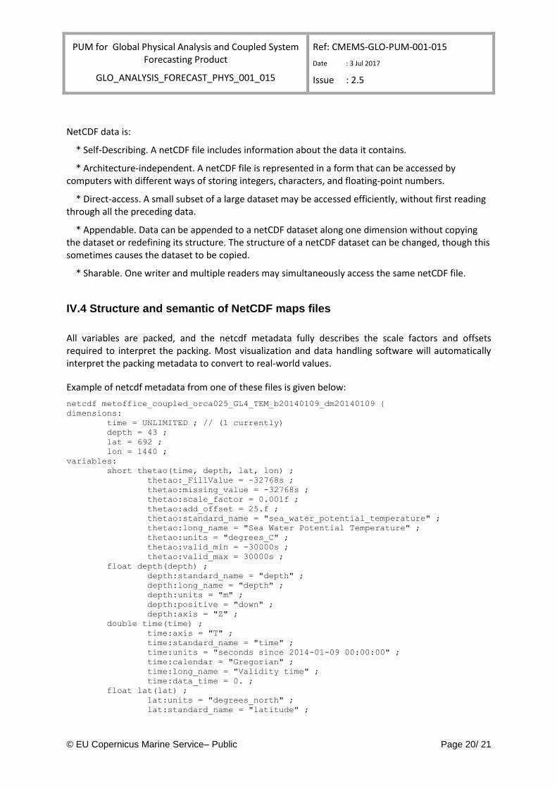
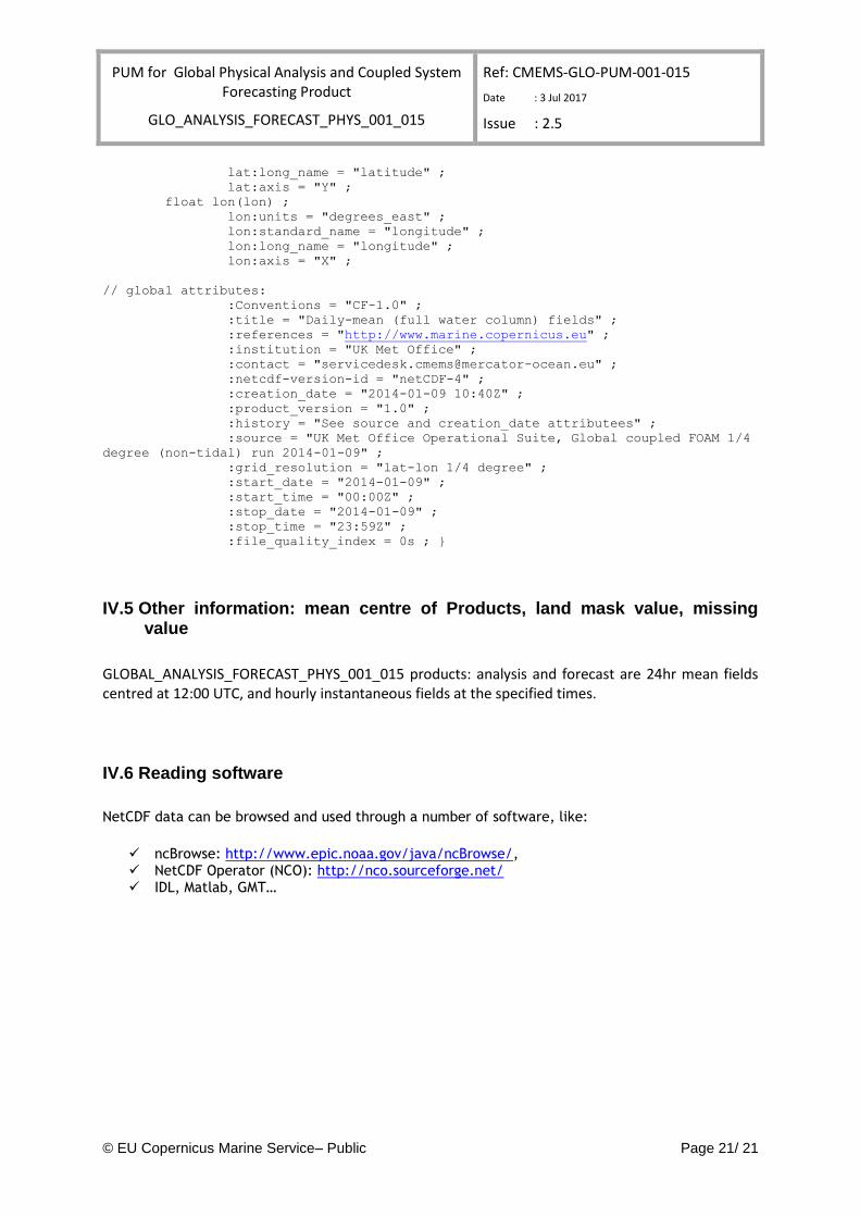
IV.4 Structure and semantic of NetCDF maps files

All variables are packed, and the netcdf metadata fully describes the scale factors and offsets required to interpret the packing. Most visualization and data handling software will automatically interpret the packing metadata to convert to real-world values.

Example of netcdf metadata from one of these files is given below:

netcdf metoffice_coupled_orca025_GL4_TEM_b20140109_dm20140109 {

dimensions:

time = UNLIMITED ; // (1 currently)

depth = 43 ;

lat = 692 ;

lon = 1440 ;

variables:

short thetao(time, depth, lat, lon) ;

thetao:_FillValue = -32768s ;

thetao:missing_value = -32768s ;

thetao:scale_factor = 0.001f ;

thetao:add_offset = 25.f ;

thetao:standard_name = "sea_water_potential_temperature" ;

thetao:long_name = "Sea Water Potential Temperature" ;

thetao:units = "degrees_C" ;

thetao:valid_min = -30000s ;

thetao:valid_max = 30000s ;

float depth(depth) ;

depth:standard_name = "depth" ;

depth:long_name = "depth" ;

depth:units = "m" ;

depth:positive = "down" ;

depth:axis = "Z" ;

double time(time) ;

time:axis = "T" ;

time:standard_name = "time" ;

time:units = "seconds since 2014-01-09 00:00:00" ;

time:calendar = "Gregorian" ;

time:long_name = "Validity time" ;

time:data_time = 0. ;

float lat(lat) ;

lat:units = "degrees_north" ;

lat:standard_name = "latitude" ;




Date : 3 Jul 2017

Issue : 2.5


lat:long_name = "latitude" ;

lat:axis = "Y" ;

float lon(lon) ;

lon:units = "degrees_east" ;

lon:standard_name = "longitude" ;

lon:long_name = "longitude" ;

lon:axis = "X" ;

// global attributes:

:Conventions = "CF-1.0" ;

:title = "Daily-mean (full water column) fields" ;

:references = "http://www.marine.copernicus.eu" ;

:institution = "UK Met Office" ;

:contact = "[email protected]" ;

:netcdf-version-id = "netCDF-4" ;

:creation_date = "2014-01-09 10:40Z" ;

:product_version = "1.0" ;

:history = "See source and creation_date attributees" ;

:source = "UK Met Office Operational Suite, Global coupled FOAM 1/4

degree (non-tidal) run 2014-01-09" ;

:grid_resolution = "lat-lon 1/4 degree" ;

:start_date = "2014-01-09" ;

:start_time = "00:00Z" ;

:stop_date = "2014-01-09" ;

:stop_time = "23:59Z" ;

:file_quality_index = 0s ; }

IV.5 Other information: mean centre of Products, land mask value, missing value

GLOBAL_ANALYSIS_FORECAST_PHYS_001_015 products: analysis and forecast are 24hr mean fields centred at 12:00 UTC, and hourly instantaneous fields at the specified times.

IV.6 Reading software

NetCDF data can be browsed and used through a number of software, like:

ncBrowse: http://www.epic.noaa.gov/java/ncBrowse/, NetCDF Operator (NCO): http://nco.sourceforge.net/ IDL, Matlab, GMT…

http://www.epic.noaa.gov/java/ncBrowse/

http://nco.sourceforge.net/

Documents

PRODUCT USER MANUAL For Global Physical Analysis …cmems-resources.cls.fr/documents/PUM/CMEMS-GLO-PUM-001-015.pdf · For Global Physical Analysis and Coupled System Forecasting Product