Embed Size (px)
Citation preview
Chapter 2The PERT/CPM Technique
Abstract Completing a project on time and within budget is not an easy task. Theproject scheduling phase plays a central role in predicting both the time and costaspects of a project. More precisely, it determines a timetable in order to be able topredict the expected time and cost of each individual activity.
In this chapter, the basic critical path calculations of a project schedule arehighlighted and the fundamental concept of an activity network is presented.Throughout all chapters of Part I, it is assumed that a project is not subject to alimited amount of resources. The project is structured in a network to model theprecedences between the various project activities. The basic concepts of projectnetwork analysis are outlined and the Program Evaluation and Review Technique(PERT) is discussed as an easy yet effective scheduling tool for projects withvariability in the activity duration estimates.
2.1 Introduction
In this chapter, the basic concepts of the definition phase (Sect. 2.2) and thescheduling phase (Sect. 2.3) of the project life cycle are discussed. It is assumedthat projects belong to the first quadrant of the project mapping matrix of Fig. 1.4and hence are assumed to have no resource limits and a low level of uncertainty.
The chapter aims to give answers to fundamental questions, such as:
• What is the expected project finish date?• How can precedence relations between activities be modeled in a network?• What are the expected activity start and finish times?• What is the effect of variability in activity time estimates on the project duration?
M. Vanhoucke, Project Management with Dynamic Scheduling,DOI 10.1007/978-3-642-25175-7 2, © Springer-Verlag Berlin Heidelberg 2012
11
12 2 The PERT/CPM Technique
2.2 Project Definition Phase
In the definition phase of a project’s life cycle, the organization defines the projectobjectives, the project specifications and requirements and the organization of theentire project. In doing so, the organization decides on how it is going to achieve allproject objectives.
The Work Breakdown Structure (WBS) is a fundamental concept of the definitionphase that, along with the Organizational Breakdown Structure (OBS), identifies theset of activities needed to achieve the project goal as well as the responsibilities ofthe project team for the various subparts of the project.
This information needs to be transformed into a network diagram that identifiesa list of project activities and the technological links with the other activities. Thisproject network is an easy and accessible tool for the critical path calculations todetermine the earliest and latest activity start times of the scheduling phase.
2.2.1 WBS and OBS
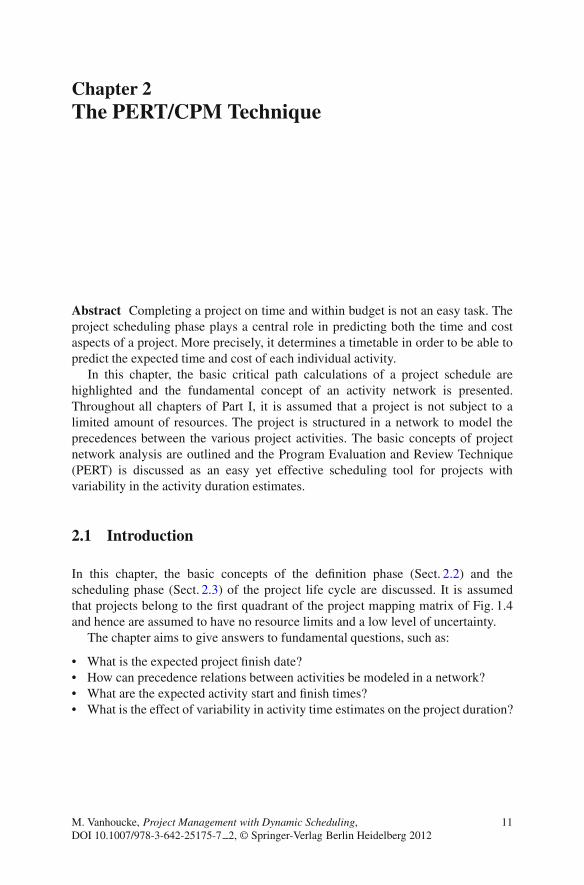
The preparation of a Work Breakdown Structure (WBS) is an important step inmanaging and mastering the inherent complexity of the project. It involves thedecomposition of major project deliverables into smaller, more manageable com-ponents until the deliverables are defined in sufficient detail to support developmentof project activities (PMBOK 2004). The WBS is a tool that defines the project andgroups the project’s discrete work elements to help organize and define the totalwork scope of the project. It provides the necessary framework for detailed costestimation and control along with providing guidance for schedule development andcontrol. Each descending level of the WBS represents an increased level of detaileddefinition of the project work.
The WBS is often displayed graphically as a hierarchical tree. It has multiplelevels of detail, as displayed in Fig. 2.1.
Project Objective
Work Items
Work Packages
Activities
Break down the project into manageable pieces (items)
The lowest-level items of any branch is a work package. Monitor and collect cost data at this level
Represent each work package by one or more activities
Fig. 2.1 Four levels of a Work Breakdown Structure
2.2 Project Definition Phase 13
• Project objective: The project objective consists of a short description of thescope of the project. A careful scope definition is of crucial importance in projectmanagement.
• Work item: The project is broken down into manageable pieces (items) to be ableto cope with the project complexity.
• Work package: The monitoring and collection of cost data often occurs at thislevel.
• Activity: The lowest level of the WBS, where the accuracy of cost, duration andresource estimates can be improved, and where the precedence relations can beincorporated.
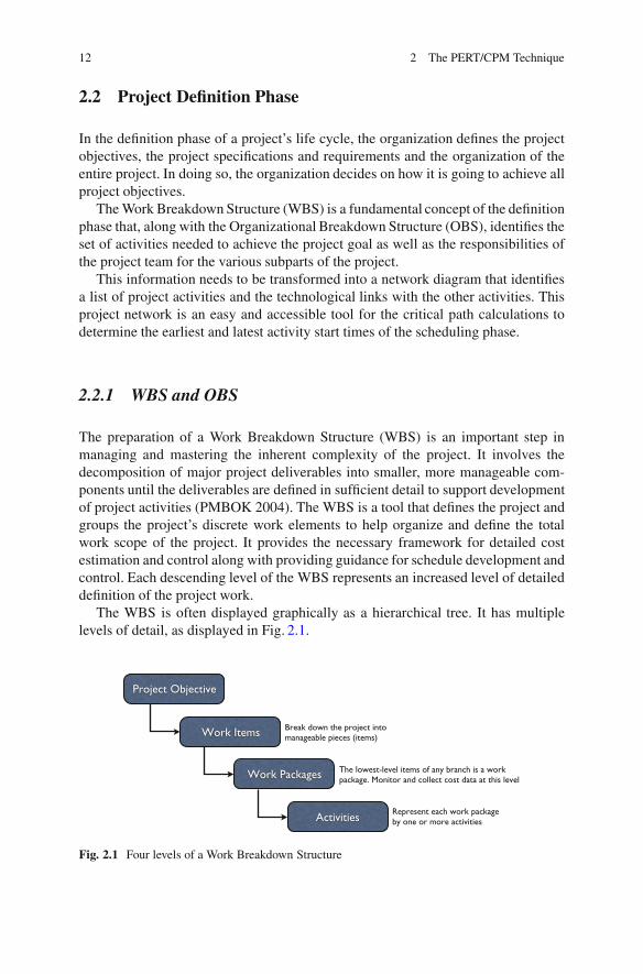
The WBS is often used in conjunction with the Organizational BreakdownStructure (OBS). The OBS indicates the organizational relationships and is usedas the framework for assigning work responsibilities. The WBS and the OBSare merged to create a Responsibility Assignment Matrix (RAM) for the projectmanager. The RAM displays the lower levels of both the WBS and the OBS andidentifies specific responsibilities for specific project tasks. It is at this point that theproject manager develops control accounts or work packages.
Figure 2.2 shows a graphical picture of a WBS/OBS conjunction and shows theRAM for a fictitious project. In the figure, the RAM uses the lowest level of the
WBS
x x x
x x
x x x x
x x x
x x x
x x x
ProjectObjective
WorkItem
WorkItem
Workpackage
Workpackage
Workpackage
Workpackage
ProjectObjective
Activity10
Activity1
Activity4
Activity9
Activity3
Activity6
Activity2
Activity5
Activity7
Activity8
RAM
OBS
Pro
ject
Obj
ectiv
e
Per
son
AP
erso
n B
Per
son
CP
erso
n C
Pro
ject
Team
2Te
am 1
Team
4Te
am 3
Team
5Te
am 6
Fig. 2.2 A Responsibility Assignment Matrix (RAM)
14 2 The PERT/CPM Technique
WBS (activity level) and OBS and defines the specific person/department from theOBS assigned to be responsible for completing the activity from the WBS (indicatedby an ‘x’). Obviously, in practice, the responsibilities are often assigned to higherWBS levels (work package or work item level).
An illustration of a WBS is given in Chap. 4 of this book. The assignmentsand scheduling of resources from the OBS to the project activities is extensivelydiscussed in the resource-constrained scheduling techniques of Chaps. 7 and 8.
2.2.2 Network Analysis
In order to construct a complete and detailed WBS, the work packages of a WBSneed to be further subdivided into activities. In doing so, it might improve thelevel of detail and accuracy of cost, duration and resource estimates which serveas inputs for the construction of a project network and scheduling phase. Note thata clear distinction between the project definition phase and the project schedulingphase will be made throughout this chapter. The definition phase, which determinesthe list of activities, the precedence relations, possible resource requirements andthe major milestones of the project, is different from the scheduling phase in thelevel of detail and the timing of project activities. Indeed, the scheduling phaseaims at the determination of start and finish times of each activity of the project,and consequently, determines the milestones in detail. This can only be done afterthe construction of the network in the definition phase. Therefore, the activitydescription with the corresponding WBS-code and the estimates for its duration,cost and resource requirement are the main outputs of the definition phase and serveas inputs for the scheduling phase. In the latter phase, the earliest and latest possiblestart (and finish) time will be determined, given the technological precedencerelations and limited resource constraints. The construction of a project schedulebased on a project network with precedence relations is discussed in Sect. 2.3 ofthis chapter, while the introduction of resources in a project network is the topic ofPart II of this book.
Many activities involve a logical sequence during execution. The links betweenthe various activities to incorporate these logical sequences are called technologicalprecedence relations. The annex technological is used to distinguish with the so-called resource relations, which will be introduced in Chaps. 7 and 8. Incorporatingthese technological links between any pair of activities is a first step in the construc-tion of the project network. A network consists of nodes and arcs and incorporatesall the activities and their technological precedence relations. A network can beseen as a graph G(N, A) where the set N is used to denote the set of nodes and A todenote the set of arcs. The network has a single start node and a single end nodeand is used as an input for the scheduling phase as discussed in Sect. 2.3. The setof activities of a project and their corresponding technological precedence relationscan be displayed as a network using two formats: an activity-on-the-node (AoN)
2.2 Project Definition Phase 15
and an activity-on-the-arc (AoA) representation. In the next subsections, these twoformats are discussed in more detail.
Activity-on-the-Arc (AoA)
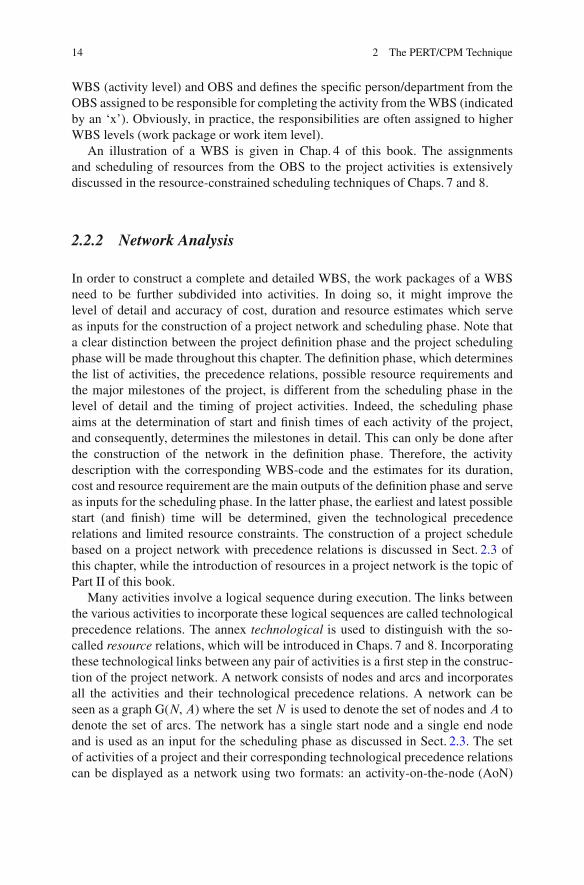
In an AoA format, activities are displayed by means of arcs in the network. Thenodes are events (or milestones) denoting the start and/or finish of a set of activitiesof the project. The technological link between activity i and activity j can bedisplayed as in Fig. 2.3. Since activities can be labeled with their correspondingstart and end node event, it is said that activity (2,3) is a successor of activity (1,2)and activity (1,2) is a predecessor of activity (2,3).
Moder et al. (1983) have suggested six rules to construct AoA networks, asfollows:
1. Before any activity may begin, all activities preceding it must be completed.2. Arrows imply logical precedence only. Neither the length nor its “compass”
direction have any difference.3. Event numbers must not be duplicated in a network.4. Any two events may be directly connected by no more than one activity.5. Networks may have only one initial event (with no predecessor) and only one
terminal event (with no successor).6. The introduction of dummy activities is often necessary to model all precedence
relations.
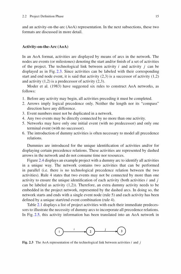
Dummies are introduced for the unique identification of activities and/or fordisplaying certain precedence relations. These activities are represented by dashedarrows in the network and do not consume time nor resources.
Figure 2.4 displays an example project with a dummy arc to identify all activitiesin a unique way. The network contains two activities that can be performedin parallel (i.e. there is no technological precedence relation between the twoactivities). Rule 4 states that two events may not be connected by more than oneactivity to ensure the unique identification of each activity (both activities i and j
can be labeled as activity (1,2)). Therefore, an extra dummy activity needs to beembedded in the project network, represented by the dashed arcs. In doing so, thenetwork starts and ends with a single event node (rule 5) and each activity has beendefined by a unique start/end event combination (rule 4).
Table 2.1 displays a list of project activities with each their immediate predeces-sors to illustrate the necessity of dummy arcs to incorporate all precedence relations.In Fig. 2.5, this activity information has been translated into an AoA network in
1 2 3i j
Fig. 2.3 The AoA representation of the technological link between activities i and j
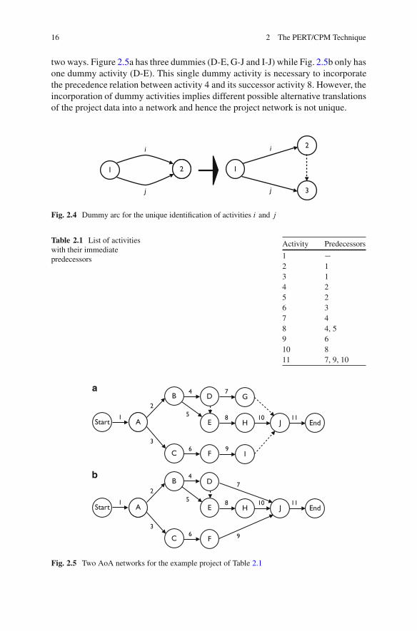
16 2 The PERT/CPM Technique
two ways. Figure 2.5a has three dummies (D-E, G-J and I-J) while Fig. 2.5b only hasone dummy activity (D-E). This single dummy activity is necessary to incorporatethe precedence relation between activity 4 and its successor activity 8. However, theincorporation of dummy activities implies different possible alternative translationsof the project data into a network and hence the project network is not unique.
1 j2
3
i
j
1
2i
j
Fig. 2.4 Dummy arc for the unique identification of activities i and j
Table 2.1 List of activitieswith their immediatepredecessors
Activity Predecessors
1 �2 13 14 25 26 37 48 4, 59 610 811 7, 9, 10
E1
Start 3A
B
C F I
D G
H J End
2
3
4 7
5 8 10
6 9
11
4
E1
Start 3A
B
C F
D
H J End
2
3
7
5 8 10
6 9
11
a
b
Fig. 2.5 Two AoA networks for the example project of Table 2.1
2.2 Project Definition Phase 17
The introduction of dummy activities, which leads to different network represen-tations of the same project, unnecessarily increases the project network complexity.Many researchers have focused on the development of (complex) algorithms tominimize the number of dummy activities in an AoA network. These algorithmsare, due to their inherent complexity, outside the scope of this book. However,Wiest and Levy (1977) have presented some guidelines for reducing the number ofdummy activities. Although these guidelines do not aim at minimizing the numberof dummy activities in an AoA network, they can be very helpful in reducingsuperfluous dummy activities and hence, the project network complexity. The rulesare as follows:
1. If a dummy node is the only activity emanating from its initial node, it can beremoved.
2. If a dummy activity is the only activity going into its final node, it also can beremoved.
3. If two (or more) activities have identical sets of predecessors (successors) thenthe two jobs should emanate from a single node connected to their predecessors(successors) by dummy activities.
4. Dummy jobs that show predecessor relations already implied by other activitiesmay be removed as redundant.
As an example, the first rule was used to reduce the number of dummy activitiesfrom 3 to 1 in Fig. 2.5.
Activity-on-the-Node (AoN)
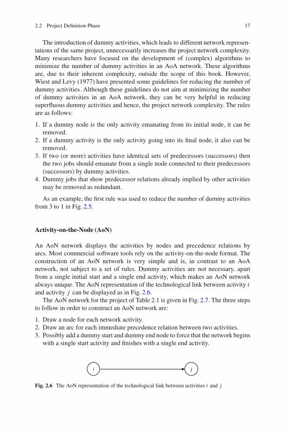
An AoN network displays the activities by nodes and precedence relations byarcs. Most commercial software tools rely on the activity-on-the-node format. Theconstruction of an AoN network is very simple and is, in contrast to an AoAnetwork, not subject to a set of rules. Dummy activities are not necessary, apartfrom a single initial start and a single end activity, which makes an AoN networkalways unique. The AoN representation of the technological link between activity i
and activity j can be displayed as in Fig. 2.6.The AoN network for the project of Table 2.1 is given in Fig. 2.7. The three steps
to follow in order to construct an AoN network are:
1. Draw a node for each network activity.2. Draw an arc for each immediate precedence relation between two activities.3. Possibly add a dummy start and dummy end node to force that the network begins
with a single start activity and finishes with a single end activity.
i j
Fig. 2.6 The AoN representation of the technological link between activities i and j
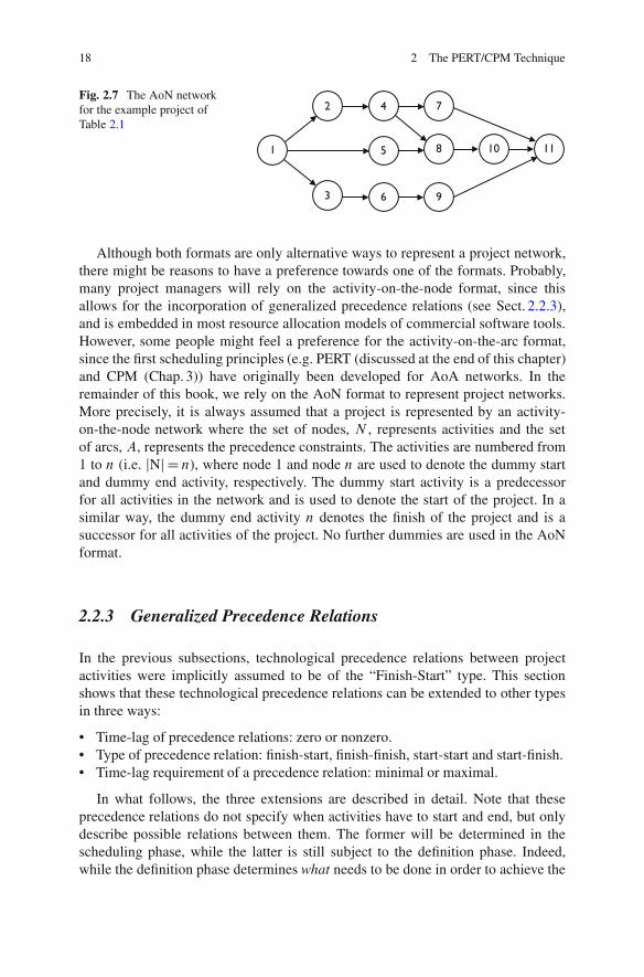
18 2 The PERT/CPM Technique
1
3
8
6
2
105
4
11
7
9
Fig. 2.7 The AoN networkfor the example project ofTable 2.1
Although both formats are only alternative ways to represent a project network,there might be reasons to have a preference towards one of the formats. Probably,many project managers will rely on the activity-on-the-node format, since thisallows for the incorporation of generalized precedence relations (see Sect. 2.2.3),and is embedded in most resource allocation models of commercial software tools.However, some people might feel a preference for the activity-on-the-arc format,since the first scheduling principles (e.g. PERT (discussed at the end of this chapter)and CPM (Chap. 3)) have originally been developed for AoA networks. In theremainder of this book, we rely on the AoN format to represent project networks.More precisely, it is always assumed that a project is represented by an activity-on-the-node network where the set of nodes, N , represents activities and the setof arcs, A, represents the precedence constraints. The activities are numbered from1 to n (i.e. jNj D n), where node 1 and node n are used to denote the dummy startand dummy end activity, respectively. The dummy start activity is a predecessorfor all activities in the network and is used to denote the start of the project. In asimilar way, the dummy end activity n denotes the finish of the project and is asuccessor for all activities of the project. No further dummies are used in the AoNformat.
2.2.3 Generalized Precedence Relations
In the previous subsections, technological precedence relations between projectactivities were implicitly assumed to be of the “Finish-Start” type. This sectionshows that these technological precedence relations can be extended to other typesin three ways:
• Time-lag of precedence relations: zero or nonzero.• Type of precedence relation: finish-start, finish-finish, start-start and start-finish.• Time-lag requirement of a precedence relation: minimal or maximal.
In what follows, the three extensions are described in detail. Note that theseprecedence relations do not specify when activities have to start and end, but onlydescribe possible relations between them. The former will be determined in thescheduling phase, while the latter is still subject to the definition phase. Indeed,while the definition phase determines what needs to be done in order to achieve the
2.2 Project Definition Phase 19
project goals, the scheduling phase determines when all these necessary steps needto be performed.
Time-Lag
A finish-start relation with a zero time-lag can be represented as follows:
FSij
Activity j can only start after the finish of activity i
A zero time-lag implies that the second activity j can start immediately after thefinish of the first activity i , or later. It does not force the immediate start after thefinish of the first activity, since the definition phase only describes the technologicalrequirements and limitations and does not aim at the construction of a timetable.
A finish-start relation with a nonzero time-lag can be represented as follows:
FSij D n
Activity j can only start n time periods after the finish of activity i
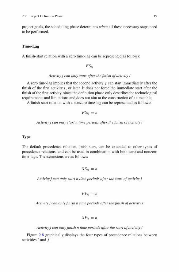
Type
The default precedence relation, finish-start, can be extended to other types ofprecedence relations, and can be used in combination with both zero and nonzerotime-lags. The extensions are as follows:
SSij D n
Activity j can only start n time periods after the start of activity i
FFij D n
Activity j can only finish n time periods after the finish of activity i
SFij D n
Activity j can only finish n time periods after the start of activity i
Figure 2.8 graphically displays the four types of precedence relations betweenactivities i and j .
20 2 The PERT/CPM Technique
i j
i j
i j
i j
SS
FF
SF
FS
Fig. 2.8 Four types ofprecedence relations betweenactivities i and j
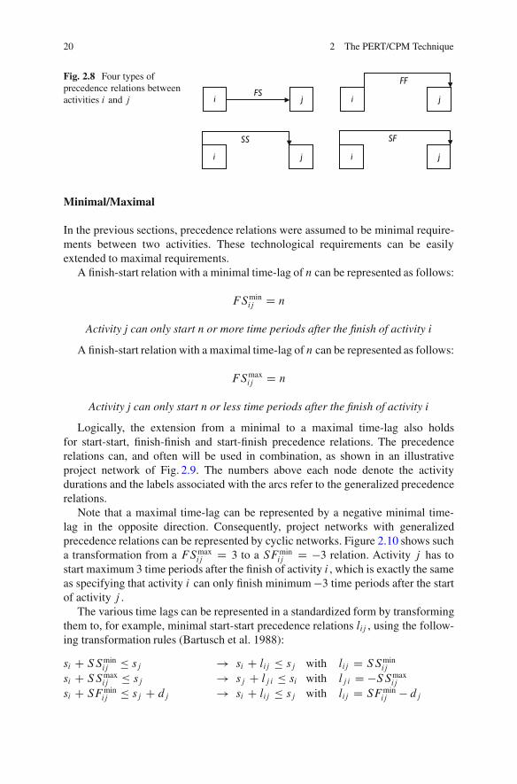
Minimal/Maximal
In the previous sections, precedence relations were assumed to be minimal require-ments between two activities. These technological requirements can be easilyextended to maximal requirements.
A finish-start relation with a minimal time-lag of n can be represented as follows:
FSminij D n
Activity j can only start n or more time periods after the finish of activity i
A finish-start relation with a maximal time-lag of n can be represented as follows:
FSmaxij D n
Activity j can only start n or less time periods after the finish of activity i
Logically, the extension from a minimal to a maximal time-lag also holdsfor start-start, finish-finish and start-finish precedence relations. The precedencerelations can, and often will be used in combination, as shown in an illustrativeproject network of Fig. 2.9. The numbers above each node denote the activitydurations and the labels associated with the arcs refer to the generalized precedencerelations.
Note that a maximal time-lag can be represented by a negative minimal time-lag in the opposite direction. Consequently, project networks with generalizedprecedence relations can be represented by cyclic networks. Figure 2.10 shows sucha transformation from a FSmax
ij D 3 to a SF minij D �3 relation. Activity j has to
start maximum 3 time periods after the finish of activity i , which is exactly the sameas specifying that activity i can only finish minimum �3 time periods after the startof activity j .
The various time lags can be represented in a standardized form by transformingthem to, for example, minimal start-start precedence relations lij , using the follow-ing transformation rules (Bartusch et al. 1988):
si C SSminij � sj ! si C lij � sj with lij D SSmin
ij
si C SSmaxij � sj ! sj C lj i � si with lj i D �SSmax
ij
si C SF minij � sj C dj ! si C lij � sj with lij D SF min
ij � dj
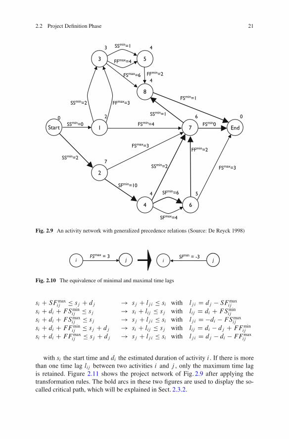
2.2 Project Definition Phase 21
0
Start
2
1
6
7
7
2
4
4
5
6
3
3
4
5
4
8
0
End
FFmax=3
FFmax=4
FSmax=6
FSmin=4
FSmax=3
FSmax=3
SFmax=4
FSmin=1
FSmin0
FFmin=2
FFmin=2
SSmin=2
SSmin=1
SSmin=1
SSmin=2
SSmin=0
SFmin=10SFmin=6
SSmin=2
Fig. 2.9 An activity network with generalized precedence relations (Source: De Reyck 1998)
i jjFSmax = 3
i jjSFmin = -3
Fig. 2.10 The equivalence of minimal and maximal time lags
si C SF maxij � sj C dj ! sj C lj i � si with lj i D dj � SF max
ij
si C di C FSminij � sj ! si C lij � sj with lij D di C FSmin
ij
si C di C FSmaxij � sj ! sj C lj i � si with lj i D �di � FSmax
ij
si C di C FF minij � sj C dj ! si C lij � sj with lij D di � dj C FF min
ij
si C di C FF maxij � sj C dj ! sj C lj i � si with lj i D dj � di � FF max
ij
with si the start time and di the estimated duration of activity i . If there is morethan one time lag lij between two activities i and j , only the maximum time lagis retained. Figure 2.11 shows the project network of Fig. 2.9 after applying thetransformation rules. The bold arcs in these two figures are used to display the so-called critical path, which will be explained in Sect. 2.3.2.
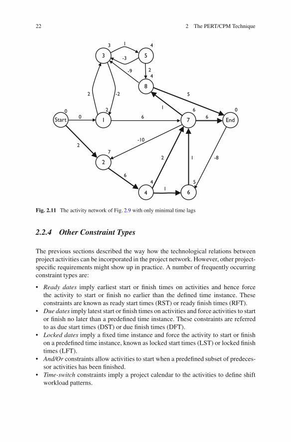
22 2 The PERT/CPM Technique
0
Start
2
1
6
7
7
2
4
4
5
6
3
3
4
5
4
8
0
End
1
-3
-9 2
-22
0 6
5
1
6
-812
-102
6
1
Fig. 2.11 The activity network of Fig. 2.9 with only minimal time lags
2.2.4 Other Constraint Types
The previous sections described the way how the technological relations betweenproject activities can be incorporated in the project network. However, other project-specific requirements might show up in practice. A number of frequently occurringconstraint types are:
• Ready dates imply earliest start or finish times on activities and hence forcethe activity to start or finish no earlier than the defined time instance. Theseconstraints are known as ready start times (RST) or ready finish times (RFT).
• Due dates imply latest start or finish times on activities and force activities to startor finish no later than a predefined time instance. These constraints are referredto as due start times (DST) or due finish times (DFT).
• Locked dates imply a fixed time instance and force the activity to start or finishon a predefined time instance, known as locked start times (LST) or locked finishtimes (LFT).
• And/Or constraints allow activities to start when a predefined subset of predeces-sor activities has been finished.
• Time-switch constraints imply a project calendar to the activities to define shiftworkload patterns.
2.3 Project Scheduling Phase 23
This nonexhaustive list can be easily extended, depending on the specific needsand requirements of the project. Many of these constraint types can be incorporatedin an AoN project network by adding extra arcs in the network. Ready times, forexample, can be incorporated in the network by adding an arc (dummy start, i )of type SSmin
1;i D ri with ri the ready time of activity i . In doing so, activityi can not start earlier than time instance ri . A natural generalization of ordinaryprecedence constraints are so-called and/or precedence constraints. In the defaultand constraint, an activity must wait for all its predecessors while in an or constraint,an activity has to wait for at least one of its predecessors. A complete description ofall possible constraint types is outside the scope of this chapter.
Time-switch constraints have been introduced as a logical extension to thetraditional models in which it is assumed that an activity can start at any timeafter the finish of all its predecessors. To that purpose, two improvements overthe traditional activity networks have been introduced by including two types oftime constraints. Time-window constraints assume that an activity can only startwithin a specified time interval. Time-schedule constraints assume that an activitycan only begin at one of an ordered schedule of beginning times. Moreover, thesetime constraints can be extended by treating time as a repeating cycle where eachcycle consists of two categories: (1) some pairs of rest and work windows and(2) a leading number specifying the maximal number of times each pair should iter-ate. By incorporating these so-called time-switch constraints, activities are forced tostart in a specific time interval and to be down in some specified rest interval. A typ-ical example of a time-switch constraint is a regular working day: work intervals aretime intervals between 9 and 12 a.m. and 1 and 5 p.m. while all the time outside thesetwo intervals is denoted as rest intervals (Vanhoucke et al. 2002; Vanhoucke 2005).
A shift-pattern is very widely used by many companies and can be consideredas a special type of time-switch constraints that force activities to start in a specifictime period and which impose three different work/rest patterns:
• day-pattern: an activity can only be executed during day time, from Mondaytill Friday. This pattern may be imposed when many persons are involved inexecuting the activity.
• d&n-pattern: an activity can be executed during the day or night, from Mondaytill Friday. This pattern may be followed in situations where activities requireonly one person who has to control the execution of the activity once in a while.
• dnw-pattern: an activity can be in execution every day or night and also duringthe weekend. This may be the case for activities that do not require humanintermission.
2.3 Project Scheduling Phase
The project network diagram and the activity time estimates made by the projectmanager during the definition phase will be used as inputs for the scheduling phase.The scheduling phase aims at the construction of a timetable to determine the
24 2 The PERT/CPM Technique
activity start and finish times and to determine a realistic total project duration withinthe limitations of the precedence relations and other constraint types. Although theminimization of the project lead time is often the most important objective duringthe scheduling phase, other scheduling objective are often crucial from a practicalpoint of view. In this chapter, only a time objective is taken into account. Theextension to other scheduling objectives is the topic of Chaps. 7 and 8.
2.3.1 Introduction to Scheduling
Scheduling is an inexact process that tries to predict the future. More precisely,it aims at the construction of a timetable for the project where start and finishtimes are assigned to the individual project activities. Since activities are subject toseveral (precedence and resource-related) constraints, the construction of a schedulecan be enormously complex. Indeed, project activities are precedence related andtheir execution may require the use of different types of resources (money, crew,equipment, . . . ). The scheduling objectives (often referred to as a measure ofperformance) may take many forms (minimizing project duration, minimizingproject costs, maximizing project revenues, optimizing due date performance, . . . ).
The early endeavors of project management and scheduling date back to thedevelopment of the Gantt chart by Henry Gantt (1861–1919). This chartingsystem for production scheduling formed the basis for two scheduling techniques,which were developed to assist in planning, managing and controlling complexorganizations: the Critical path Method (CPM) and Program Evaluation and ReviewTechnique (PERT). The Gantt chart is a horizontal-bar schedule showing activitystart, duration, and completion.
The Critical Path Method was the discovery of M. R. Walker of E. I. Du Pontde Nemours and Co. and J. E. Kelly of Remington Rand, circa 1957. The first testwas made in 1958, when CPM was applied to the construction of a new chemicalplant. In March 1959, the method was applied to a maintenance shut-down at the DuPont works in Louisville, Kentucky. The Program Evaluation and Review Techniquewas devised in 1958 for the POLARIS missile program by the program evaluationbranch of the special projects office of the U.S. Navy. Due to the similarities of bothtechniques, they are often referred to as the PERT/CPM technique.
Thanks to the development of the personal computer, project scheduling algo-rithms started to shift to resource allocation models and the development of softwarewith resource-constrained scheduling features (see Chaps. 7 and 8). From the 1990son, numerous extensions of resource allocations and the development of tools (e.g.the CC/BM approach of Chap. 10) allowed the project manager to deal with bothcomplexity and uncertainty at the same time (see the project mapping picture ofFig. 1.4).
In this chapter, the basic critical path calculations are discussed where it isassumed that projects are not subject to limited availability of resources and thescheduler follows a time-perspective scheduling objective. In Sect. 2.4, the Program
2.3 Project Scheduling Phase 25
Evaluation and Review Technique is discussed, which extends the time objectiveof a schedule to probability calculations. In Part II of this book, the schedulingprinciples will be extended to projects with limited resource availabilities andscheduling objectives different from time minimization will be discussed.
2.3.2 Critical Path Calculations
Consider the data of Table 2.2 for a fictitious project with 12 nondummy activities(and a dummy start (1) and end (14) activity). The sets Pi and Si are used to referto the direct predecessors and successors of an activity i . Note that precedencerelations will be of the FSmin
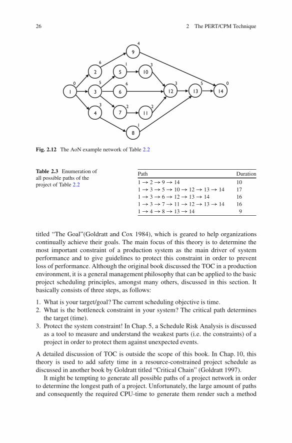
ij D 0 type, unless indicated otherwise. All modelsand principles discussed throughout the chapters can be extended to generalizedprecedence relations between project activities, resulting in an increase in complex-ity but not in a fundamental difference in scheduling approach. Figure 2.12 displaysthe AoN network of Table 2.2, where the number above the node denotes the activityduration.
A path in a network can be defined as a series of connected activities from thestart to the end of the project. All activities (and consequently, all paths) mustbe completed to finish the project. Table 2.3 enumerates all possible paths of theexample network of Fig. 2.12, with their corresponding total duration.
The earliest possible completion time of the project is equal to the longest path inthe network. This path, referred to as the critical path, determines the overall projectduration. Care must be taken to keep these activities on schedule, since delays in anyof these activities result in a violation of the entire project duration.
The clever reader immediately recognizes the basic principle underlying theTheory Of Constraints (TOC) introduced by Dr. Eliyahu M. Goldratt in his book
Table 2.2 A fictitiousproject example with 12nondummy activities
Activity Predecessors Duration (days)
1 � 02 1 63 1 54 1 35 3 16 3 37 3 28 4 19 2 410 5 311 7 112 6, 10, 11 313 8, 12 514 9, 13 0
26 2 The PERT/CPM Technique
6
3 2 2
3
1 3
2
4 7
12
11
5
136
10
9
8
14
5 6
1
4
1
3
5 00
Fig. 2.12 The AoN example network of Table 2.2
Table 2.3 Enumeration ofall possible paths of theproject of Table 2.2
Path Duration
1 ! 2 ! 9 ! 14 101 ! 3 ! 5 ! 10 ! 12 ! 13 ! 14 171 ! 3 ! 6 ! 12 ! 13 ! 14 161 ! 3 ! 7 ! 11 ! 12 ! 13 ! 14 161 ! 4 ! 8 ! 13 ! 14 9
titled “The Goal”(Goldratt and Cox 1984), which is geared to help organizationscontinually achieve their goals. The main focus of this theory is to determine themost important constraint of a production system as the main driver of systemperformance and to give guidelines to protect this constraint in order to preventloss of performance. Although the original book discussed the TOC in a productionenvironment, it is a general management philosophy that can be applied to the basicproject scheduling principles, amongst many others, discussed in this section. Itbasically consists of three steps, as follows:
1. What is your target/goal? The current scheduling objective is time.2. What is the bottleneck constraint in your system? The critical path determines
the target (time).3. Protect the system constraint! In Chap. 5, a Schedule Risk Analysis is discussed
as a tool to measure and understand the weakest parts (i.e. the constraints) of aproject in order to protect them against unexpected events.
A detailed discussion of TOC is outside the scope of this book. In Chap. 10, thistheory is used to add safety time in a resource-constrained project schedule asdiscussed in another book by Goldratt titled “Critical Chain” (Goldratt 1997).
It might be tempting to generate all possible paths of a project network in orderto determine the longest path of a project. Unfortunately, the large amount of pathsand consequently the required CPU-time to generate them render such a method
2.3 Project Scheduling Phase 27
inapplicable for networks with a realistic size. Therefore, software tools rely on athree step procedure in order to detect the critical path of a network, as follows:
1. Calculate the earliest start schedule2. Calculate the latest start schedule3. Calculate the slack for each activity
Earliest Start Schedule (ESS)
The earliest start esi of each activity i can be calculated using forward calculationsin the project network. The earliest start of an activity is equal to or larger than theearliest finish of all its predecessor activities. The earliest finish efi of an activity i
is defined as its earliest start time increased with its duration estimate.The earliest start times can be calculated using the following forward calcula-
tions, starting with the dummy start node 1:
es1 D 0
esj D max.esi C di ji 2 Pj /
and the earliest finish times are given by:
efi D esi C di
It is easy to verify that the earliest start times of the project activities of Table 2.2are given by es1 = 0, es2 = 0, es3 = 0, es4 = 0, es5 = 5, es6 = 5, es7 = 5, es8 = 3, es9 = 6,es10 = 6, es11 = 7, es12 = 9, es13 = 12 and es14 = 17. The overall minimal projectduration equals 17 time units.
Latest Start Schedule (LSS)
The latest finish lfi of each activity i can be calculated in an analogous way, usingbackward calculations, starting from the project deadline ın at the dummy end nodeof the project. The latest finish of an activity is equal to or less than the latest start ofall its successor activities. The latest start lsi of an activity i is defined as its latestfinish time decreased with its duration estimate.
The latest finish times can be calculated using the following backward calcula-tions, starting with the dummy end node n:
lfn D ın
lfi D min.lfj � dj jj 2 Si/
28 2 The PERT/CPM Technique
and the latest start times are given by:
lsi D lfi � di
Given the project deadline of 17 time units, calculated as the earliest start of theend dummy activity in the previous step, the latest start times of each activity aregiven by ls1 = 0, ls2 = 7, ls3 = 0, ls4 = 8, ls5 = 5, ls6 = 6, ls7 = 6, ls8 = 11, ls9 = 13,ls10 = 6, ls11 = 8, ls12 = 9, ls13 = 12 and ls14 = 17.
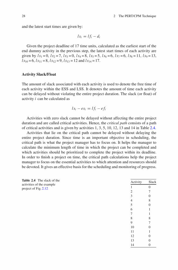
Activity Slack/Float
The amount of slack associated with each activity is used to denote the free time ofeach activity within the ESS and LSS. It denotes the amount of time each activitycan be delayed without violating the entire project duration. The slack (or float) ofactivity i can be calculated as
lsi � esi D lfi � efi
Activities with zero slack cannot be delayed without affecting the entire projectduration and are called critical activities. Hence, the critical path consists of a pathof critical activities and is given by activities 1, 3, 5, 10, 12, 13 and 14 in Table 2.4.
Activities that lie on the critical path cannot be delayed without delaying theentire project duration. Since time is an important objective in scheduling, thecritical path is what the project manager has to focus on. It helps the manager tocalculate the minimum length of time in which the project can be completed andwhich activities should be prioritized to complete the project within its deadline.In order to finish a project on time, the critical path calculations help the projectmanager to focus on the essential activities to which attention and resources shouldbe devoted. It gives an effective basis for the scheduling and monitoring of progress.
Table 2.4 The slack of theactivities of the exampleproject of Fig. 2.12
Activity Slack
1 02 73 04 85 06 17 18 89 710 011 112 013 014 0
2.3 Project Scheduling Phase 29
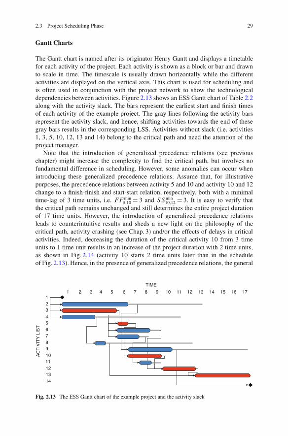
Gantt Charts
The Gantt chart is named after its originator Henry Gantt and displays a timetablefor each activity of the project. Each activity is shown as a block or bar and drawnto scale in time. The timescale is usually drawn horizontally while the differentactivities are displayed on the vertical axis. This chart is used for scheduling andis often used in conjunction with the project network to show the technologicaldependencies between activities. Figure 2.13 shows an ESS Gantt chart of Table 2.2along with the activity slack. The bars represent the earliest start and finish timesof each activity of the example project. The gray lines following the activity barsrepresent the activity slack, and hence, shifting activities towards the end of thesegray bars results in the corresponding LSS. Activities without slack (i.e. activities1, 3, 5, 10, 12, 13 and 14) belong to the critical path and need the attention of theproject manager.
Note that the introduction of generalized precedence relations (see previouschapter) might increase the complexity to find the critical path, but involves nofundamental difference in scheduling. However, some anomalies can occur whenintroducing these generalized precedence relations. Assume that, for illustrativepurposes, the precedence relations between activity 5 and 10 and activity 10 and 12change to a finish-finish and start-start relation, respectively, both with a minimaltime-lag of 3 time units, i.e. FF min
5;10 D 3 and SSmin10;12 D 3. It is easy to verify that
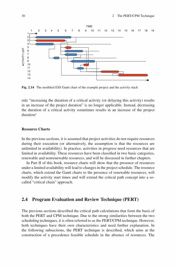
the critical path remains unchanged and still determines the entire project durationof 17 time units. However, the introduction of generalized precedence relationsleads to counterintuitive results and sheds a new light on the philosophy of thecritical path, activity crashing (see Chap. 3) and/or the effects of delays in criticalactivities. Indeed, decreasing the duration of the critical activity 10 from 3 timeunits to 1 time unit results in an increase of the project duration with 2 time units,as shown in Fig. 2.14 (activity 10 starts 2 time units later than in the scheduleof Fig. 2.13). Hence, in the presence of generalized precedence relations, the general
1234567891011121314
TIME
AC
TIV
ITY
LIS
T
1 2 3 4 5 6 7 8 9 10 11 12 13 14 15 16 17
Fig. 2.13 The ESS Gantt chart of the example project and the activity slack
30 2 The PERT/CPM Technique
1234567891011121314
TIMEA
CT
IVIT
Y L
IST
Fig. 2.14 The modified ESS Gantt chart of the example project and the activity slack
rule “increasing the duration of a critical activity (or delaying this activity) resultsin an increase of the project duration” is no longer applicable. Instead, decreasingthe duration of a critical activity sometimes results in an increase of the projectduration!
Resource Charts
In the previous sections, it is assumed that project activities do not require resourcesduring their execution (or alternatively, the assumption is that the resources areunlimited in availability). In practice, activities in progress need resources that arelimited in availability. These resources have been classified in two basic categories,renewable and nonrenewable resources, and will be discussed in further chapters.
In Part II of this book, resource charts will show that the presence of resourcesunder a limited availability will lead to changes in the project schedule. The resourcecharts, which extend the Gantt charts to the presence of renewable resources, willmodify the activity start times and will extend the critical path concept into a so-called “critical chain” approach.
2.4 Program Evaluation and Review Technique (PERT)
The previous sections described the critical path calculations that form the basis ofboth the PERT and CPM technique. Due to the strong similarities between the twoscheduling techniques, it is often referred to as the PERT/CPM technique. However,both techniques have their own characteristics and need further explanation. Inthe following subsections, the PERT technique is described, which aims at theconstruction of a precedence feasible schedule in the absence of resources. The
2.4 Program Evaluation and Review Technique (PERT) 31
details of the critical path method (CPM) are reserved for Chap. 3, where theconstruction of a precedence feasible schedule with nonrenewable resources isdiscussed.
2.4.1 Three Activity Duration Estimates
In the previous section, it was assumed that the activity duration estimates, and thederived values for the earliest start, latest start, earliest finish and latest finish wereall deterministic. In reality, this is seldom true and durations are often not known inadvance. PERT has extended this deterministic approach in the face of uncertaintyabout activity times, and employs a special formula for estimating activity durations.The approach of PERT assumes that the activity duration estimates are doneby someone who is familiar with the activity, and has enough insight in thecharacteristics of the activity. Hence, the technique requires three duration estimatesfor each individual activity, as follows:
• Optimistic time estimate: This is the shortest possible time in which the activitycan be completed, and assumes that everything has to go perfect.
• Realistic time estimate: This is the most likely time in which the activity can becompleted under normal circumstances.
• Pessimistic time estimate: This is the longest possible time the activity mightneed, and assumes a worst-case scenario.
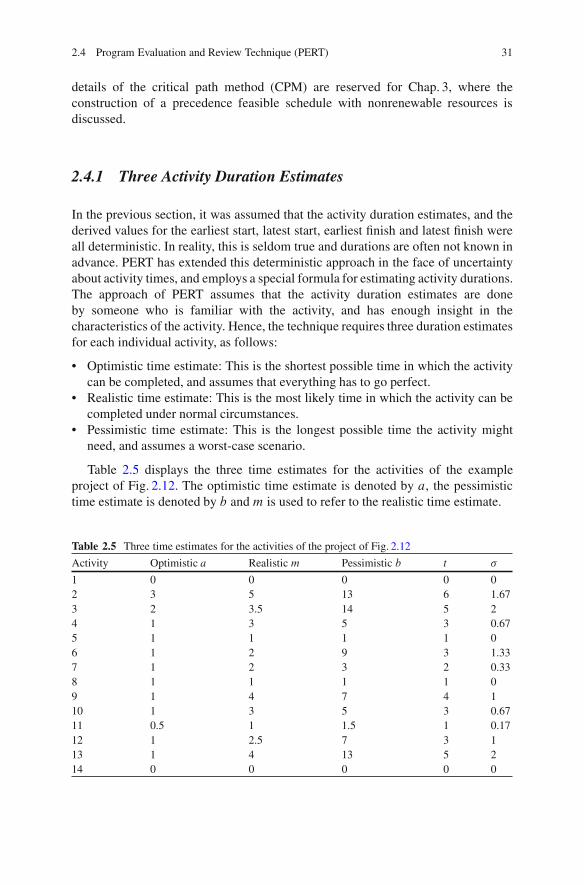
Table 2.5 displays the three time estimates for the activities of the exampleproject of Fig. 2.12. The optimistic time estimate is denoted by a, the pessimistictime estimate is denoted by b and m is used to refer to the realistic time estimate.
Table 2.5 Three time estimates for the activities of the project of Fig. 2.12
Activity Optimistic a Realistic m Pessimistic b t �
1 0 0 0 0 02 3 5 13 6 1.673 2 3.5 14 5 24 1 3 5 3 0.675 1 1 1 1 06 1 2 9 3 1.337 1 2 3 2 0.338 1 1 1 1 09 1 4 7 4 110 1 3 5 3 0.6711 0.5 1 1.5 1 0.1712 1 2.5 7 3 113 1 4 13 5 214 0 0 0 0 0
32 2 The PERT/CPM Technique
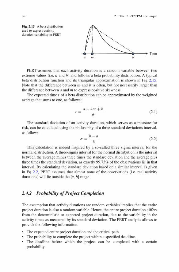
Timea bm
Fig. 2.15 A beta distributionused to express activityduration variability in PERT
PERT assumes that each activity duration is a random variable between twoextreme values (i.e. a and b) and follows a beta probability distribution. A typicalbeta distribution function and its triangular approximation is shown in Fig. 2.15.Note that the difference between m and b is often, but not necessarily larger thanthe difference between a and m to express positive skewness.
The expected time t of a beta distribution can be approximated by the weightedaverage that sums to one, as follows:
t D a C 4m C b
6(2.1)
The standard deviation of an activity duration, which serves as a measure forrisk, can be calculated using the philosophy of a three standard deviations interval,as follows:
� D b � a
6(2.2)
This calculation is indeed inspired by a so-called three sigma interval for thenormal distribution. A three-sigma interval for the normal distribution is the intervalbetween the average minus three times the standard deviation and the average plusthree times the standard deviation, as exactly 99.73% of the observations lie in thatinterval. By calculating the standard deviation based on a similar interval as givenin Eq. 2.2, PERT assumes that almost none of the observations (i.e. real activitydurations) will lie outside the Œa; b� range.
2.4.2 Probability of Project Completion
The assumption that activity durations are random variables implies that the entireproject duration is also a random variable. Hence, the entire project duration differsfrom the deterministic or expected project duration, due to the variability in theactivity times as measured by its standard deviation. The PERT analysis allows toprovide the following information:
• The expected entire project duration and the critical path.• The probability to complete the project within a specified deadline.• The deadline before which the project can be completed with a certain
probability.
2.4 Program Evaluation and Review Technique (PERT) 33
The PERT analysis calculates the expected critical path based on the expectedduration of each activity. In the example project, the expected critical path E.T /
is equal to 17 time units and consists of the activities 1, 3, 5, 10, 12, 13 and 14.Since each activity is assumed to be a random variable following a beta probabilitydistribution, the total expected duration E.T / is also a random variable with aknown distribution. This known distribution can be derived using the well-knowncentral limit theorem.
The central limit theorem states that, given a distribution with an average E.T / and varianceVar.T /, the sampling distribution of the mean approaches a normal distribution with anaverage E.T / and a variance Var.T /=n as n, the sample size, increases.
In the example project, the sample consists of the expected critical activities1, 3, 5, 10, 12, 13 and 14 with each an average duration calculated earlier. Althoughthe CLT as described above is formulated for the sampling distribution of the mean,the project completion time is simply the sum of the expected activity times for thecritical path activities and hence, a total average duration of 17 time units can becalculated. Similarly, a total variance1 that can be calculated as Var.T / D 22 C02 C 0:672 C 12 C 22 D 9:44 and, consequently, the standard deviation equalsp
9:44 D 3:07.Consequently, the example project follows a normal distribution with an average
total duration of 17 time units and a standard deviation of 3.07, i.e. N.17I 3:07/.Using normal tables, or the well-known “normdist” or “norminv” functions inMicrosoft Excel, it is easy to verify the calculations below.
Probabilities: The probability that the example project has a total duration lessthan or equal to 20 time units equals
P.T � 20/ D P
�T � 17
3:07� 20 � 17
3:07
�
D P.z � 0:976/
D 83:55%
with z the symbol for the standardized value of the normal distribution.
Percentiles: The project duration T with a risk of exceeding of 10% is equal tothe 90th percentile of the N.17I 3:07/ normal distribution and can be calculated asfollows:
90% percentile ! z D 1:28 D T � 17
3:07
! T D 20:9 time units .e:g: weeks/
1Only activities on the expected critical path are taken into account.
34 2 The PERT/CPM Technique
Confidence Intervals: The project will have a total duration between approxi-mately 10.8 and 23.1 time units with a probability of 95%, which can be calculatedas a 2� interval for the normal distribution. A more detailed statistical explanationcan be found in any statistics handbook and is outside the scope of this book.
2.4.3 Beyond PERT
Despite the relevance of the PERT planning concept, the technique has often beencriticized in literature. The PERT analysis implicitly assumes that all activities thatare not on the critical path may be ignored by setting the activity durations to theiraverage values. In realistic settings, projects have multiple critical paths instead ofa single unique critical path. Moreover, in the stochastic setting, every noncriticalpath has the potential to become critical and hence the critical path would be themaximum of a set of possible critical paths. It is also assumed that the activitydurations are independent random variables while in reality they can be dependent.These strict assumptions might lead to inaccuracies and has been the subject of a lotof research. In Chap. 5, the PERT technique is extended to Monte-Carlo simulationanalyses, which allows to analyze the distribution of the critical path without therestricted PERT assumptions. For an overview of the pitfalls of making traditionalPERT assumptions, the reader is referred to Elmaghraby (1977).
2.5 Conclusion
This chapter outlined the basic concepts of the definition and scheduling phases of aproject’s life cycle. The definition phase can be considered as the “what” phase sinceits main target is to determine what needs to be done in order to reach the projectgoal. It mainly consists of determining the main set of activities and precedencerelations (modeled in a project network) and the responsibilities of the variousproject subparts. The scheduling phase, the “when” phase, constructs a timetablefor the various project activities within a certain scheduling objective (which isassumed to be a time minimization objective in the current chapter), leading to adeterministic forecast of the earliest and latest activity start times and their slackwithin the minimal project duration.
In an attempt to add stochastic elements to the deterministic project schedule,the basic concepts of the PERT technique and an illustrative example have beendiscussed in the current chapter as a valuable tool to deal with a (low) degree ofuncertainty in activity estimates. Although the basic concepts of the critical pathscheduling approach have been outlined in this chapter, an overview of the maincharacteristics of the Critical Path Method (CPM), such as the activity time/costtrade-off function and the activity crashing possibility, is the subject of Chap. 3.

2.5 Conclusion 35
It should be noted that the usefulness of these scheduling methods should beput into the right perspective. Despite the relevance of introducing activity estimatevariability in the project schedule under strict assumptions, the PERT principleshave their inaccuracies and potential pitfalls. Consequently, the techniques dis-cussed in this chapter are classified in the first quadrant (low uncertainty/lowcomplexity) of the project mapping picture of Fig. 1.4. A project scheduling settingwith higher degree of uncertainty is the topic of Chap. 5. A higher degree ofcomplexity in project scheduling is mainly due to the introduction of a limitedresource availability, which will be discussed in Part II of this book.