Prostatome: A combined anatomical and disease based MRI atlas of the prostateMirabela Rusu, B. Nicolas Bloch, Carl C. Jaffe, Elizabeth M. Genega, Robert E. Lenkinski, Neil M. Rofsky,

Ernest Feleppa, and Anant Madabhushi

Citation: Medical Physics 41, 072301 (2014); doi: 10.1118/1.4881515 View online: http://dx.doi.org/10.1118/1.4881515 View Table of Contents: http://scitation.aip.org/content/aapm/journal/medphys/41/7?ver=pdfcov Published by the American Association of Physicists in Medicine Articles you may be interested in A dual model HU conversion from MRI intensity values within and outside of bone segment for MRI-basedradiotherapy treatment planning of prostate cancer Med. Phys. 41, 011704 (2014); 10.1118/1.4842575 3D prostate histology reconstruction: An evaluation of image-based and fiducial-based algorithms Med. Phys. 40, 093501 (2013); 10.1118/1.4816946 Multimodal CT/MR based semiautomated segmentation of rat vertebrae affected by mixed osteolytic/osteoblasticmetastases Med. Phys. 39, 2848 (2012); 10.1118/1.3703590 Elastic registration of multimodal prostate MRI and histology via multiattribute combined mutual information Med. Phys. 38, 2005 (2011); 10.1118/1.3560879 MRI/TRUS data fusion for prostate brachytherapy. Preliminary results Med. Phys. 31, 1568 (2004); 10.1118/1.1739003

Prostatome: A combined anatomical and disease based MRI atlasof the prostate

Mirabela RusuCase Western Reserve University, Cleveland, Ohio 44106

B. Nicolas Bloch and Carl C. JaffeBoston University School of Medicine, Boston, Massachusetts 02118

Elizabeth M. GenegaBeth Israel Deaconess Medical Center, Boston, Massachusetts 02215

Robert E. Lenkinski and Neil M. RofskyUT Southwestern Medical Center, Dallas, Texas 75235

Ernest FeleppaRiverside Research Institute, New York, New York 10038

Anant Madabhushia)

Case Western Reserve University, Cleveland, Ohio 44106

(Received 26 November 2013; revised 7 May 2014; accepted for publication 17 May 2014;published 17 June 2014)

Purpose: In this work, the authors introduce a novel framework, the anatomically constrained regis-tration (AnCoR) scheme and apply it to create a fused anatomic-disease atlas of the prostate which theauthors refer to as the prostatome. The prostatome combines a MRI based anatomic and a histologybased disease atlas. Statistical imaging atlases allow for the integration of information across mul-tiple scales and imaging modalities into a single canonical representation, in turn enabling a fusedanatomical-disease representation which may facilitate the characterization of disease appearancerelative to anatomic structures. While statistical atlases have been extensively developed and studiedfor the brain, approaches that have attempted to combine pathology and imaging data for study ofprostate pathology are not extant. This works seeks to address this gap.Methods: The AnCoR framework optimizes a scoring function composed of two surface (prostateand central gland) misalignment measures and one intensity-based similarity term. This ensures thecorrect mapping of anatomic regions into the atlas, even when regional MRI intensities are inconsis-tent or highly variable between subjects. The framework allows for creation of an anatomic imagingand a disease atlas, while enabling their fusion into the anatomic imaging-disease atlas. The atlas pre-sented here was constructed using 83 subjects with biopsy confirmed cancer who had pre-operativeMRI (collected at two institutions) followed by radical prostatectomy. The imaging atlas results frommapping the in vivo MRI into the canonical space, while the anatomic regions serve as domain con-straints. Elastic co-registration MRI and corresponding ex vivo histology provides “ground truth”mapping of cancer extent on in vivo imaging for 23 subjects.Results: AnCoR was evaluated relative to alternative construction strategies that use either MRI in-tensities or the prostate surface alone for registration. The AnCoR framework yielded a central glandDice similarity coefficient (DSC) of 90%, and prostate DSC of 88%, while the misalignment of theurethra and verumontanum was found to be 3.45 mm, and 4.73 mm, respectively, which were mea-sured to be significantly smaller compared to the alternative strategies. As might have been anticipatedfrom our limited cohort of biopsy confirmed cancers, the disease atlas showed that most of the tumorextent was limited to the peripheral zone. Moreover, central gland tumors were typically larger insize, possibly because they are only discernible at a much later stage.Conclusions: The authors presented the AnCoR framework to explicitly model anatomic constraintsfor the construction of a fused anatomic imaging-disease atlas. The framework was applied to con-structing a preliminary version of an anatomic-disease atlas of the prostate, the prostatome. Theprostatome could facilitate the quantitative characterization of gland morphology and imaging fea-tures of prostate cancer. These techniques, may be applied on a large sample size data set to createa fully developed prostatome that could serve as a spatial prior for targeted biopsies by urologists.Additionally, the AnCoR framework could allow for incorporation of complementary imaging andmolecular data, thereby enabling their careful correlation for population based radio-omics studies.© 2014 American Association of Physicists in Medicine. [http://dx.doi.org/10.1118/1.4881515]

Key words: anatomic imaging atlas, prostate cancer, guided biopsy, in vivo imaging, image processing

072301-1 Med. Phys. 41 (7), July 2014 © 2014 Am. Assoc. Phys. Med. 072301-10094-2405/2014/41(7)/072301/12/$30.00

072301-2 Rusu et al.: Combined anatomical and disease based MRI prostate atlas 072301-2

1. INTRODUCTION

Statistical biomedical atlases allow for the succinct encapsu-lation of structural, functional, and anatomical variability oforgans across a population within a single reference or canon-ical representation. For example, imaging data from multiplepatients may be projected into the canonical space to create astatistical imaging atlas.1, 2 This could help facilitate the char-acterization of the variation in appearance and shape of or-gan anatomy and morphology across a population. Similarly,disease atlases from imaging data have been constructed tocharacterize the 3D spatial distribution of diseases, such asprostate cancer.3, 4 These atlases could help improve interven-tional procedures, such as image guided biopsies4, 5 to samplethe organ in those regions where the atlas indicates the higherlikelihood of disease. Thus these disease atlases may serveas a priori cancer probability maps to facilitate the computerassisted diagnosis of disease.6, 7

However, these disease atlases require explicit delineationof disease presence and extent on the imaging data. Typi-cally this is only possible to do definitively on histopathol-ogy and not on in vivo imaging which does not have theresolution or sensitivity to confirm disease extent. This sug-gests that the region of disease delineated on histology needsto be mapped onto the corresponding in vivo imaging. Thismapping of disease extent from histology onto the corre-sponding in vivo imaging and then subsequently onto thecanonical space representation could allow for creation of afused anatomic imaging-disease atlas. Such fused imaging-disease atlases may further the discovery of quantitative invivo imaging biomarkers for distinguishing benign, indolent,and aggressive variations of the same disease.

In vivo imaging atlases have been previously constructedfor various organs, such as brain,1, 2 heart,8, 9 and prostate.10

Where available, histology can be fused with imaging to de-fine targets in vivo for which variations in morphology can bequantified across a population. However for the brain, avail-ability of corresponding histopathology is only possible post-mortem in healthy human subjects11 or animal models.12, 13

In the context of the prostate, relatively little work has beendone in creating imaging atlases or disease atlases.3–5, 10, 14, 15

Additionally there has been no work, that we are aware of, thathas attempted to marry the MRI and disease atlases into a sin-gle canonical representation. In this work, we attempt to com-bine an MRI based prostate atlas with a disease based atlasconstructed from histology to create a fused anatomic-diseaseatlas for the prostate, one that we refer to as the prostatome.MRI has been increasingly used over the past decade for stag-ing of prostate cancer.16–18 However, definitive validation ofthe ability of MRI to identify prostate cancer requires cor-responding histopathology. Cancer delineations on histologycan be accurately mapped onto corresponding in vivo MRIvia deformable co-registration methods.19 Histopathology isusually available in settings where men who have been di-agnosed with prostate cancer subsequently undergo a stag-ing MRI prior to radical prostatectomy. Constructing a his-tology based disease atlas based off the radical prostatectomyspecimens and then subsequently mapping the disease onto

in vivo MRI allows for precise study of variation of struc-tural, functional, and morphologic parameters within the dis-eased region. While a disease atlas (without the fusion ofcorresponding imaging) can only provide the spatial locationand distribution of the disease, an imaging atlas alone withoutthe corresponding disease mapping from histopathology willbe unable to capture the population based imaging variationswithin the diseased regions.

Creating a fused anatomic-disease atlas is replete withchallenges in the construction of the imaging atlas and dis-ease atlases, and their subsequent fusion. In the context of theprostate, the anatomic substructures of the prostate, the cen-tral gland (CG), and peripheral zone, vary greatly in shape,dimension, and imaging appearance between subjects. Suchnatural variability hinders the process of intersubject regis-tration, potentially reducing the accuracy of the imaging at-las. Moreover, the disease atlas relies on tumor ground truthdelineated on ex vivo histology which is only available forthose patients that choose radical prostatectomy as treatment.Furthermore, the MRI appearance of disease not only variesbetween subjects but is also function of spatial location ofdisease.6

To address these challenges we introduce an anatomicallyconstrained registration (AnCoR) framework to construct afused imaging-disease atlas of the prostate and its anatomicsubstructures. We refer to this fused atlas as the “prostatome.”AnCoR allows for explicit constraint based modeling of boththe central gland and prostate boundaries. The AnCoR frame-work allows for simultaneous construction of both the imag-ing and disease atlases, while ensuring the proper accuratealignment of prostatic anatomic substructures. The imagingatlas was constructed by integrating the pre-operative T2-wMRI for men with biopsy confirmed prostate cancer. The dis-ease atlas used the cancer ground truth mapped from histol-ogy onto corresponding in vivo MRI.19 The prostatome thusallows for the characterization of the tumor extent relativeto the anatomic structures of the prostate in 3D, while pro-viding a statistical model that accurately captures the vari-ation in imaging and shape of these substructures across apopulation.

In this work, the AnCoR framework was applied on datacollected from 83 subjects at two different institutions. Thefirst cohort (S1) includes 43 subjects with 3.0 Tesla (T) T2-wMRI from one institution, while the second cohort, S2, is com-posed of 40 subjects with 1.5 T T2-w MRI from a second in-stitution. Moreover, 23 subjects from the cohort S1 had wholemount histology with annotated tumor that was mapped ontocorresponding in vivo T2-w MRI using the elastic registrationapproach developed by Chappelow et al.19 The cancer anno-tations from the 23 patients were used to create the diseaseatlas.

The AnCoR framework was compared against two state ofthe art methods. One scheme employed a prostate surface3

and the second method was based off using MRI intensi-ties alone.1 Region overlap and anatomic landmark deviationwere estimated to determine the registration accuracy.

The remainder of this paper is organized as follows. Previ-ous work in atlas construction is presented in Sec. 2. In Sec. 3,

Medical Physics, Vol. 41, No. 7, July 2014

072301-3 Rusu et al.: Combined anatomical and disease based MRI prostate atlas 072301-3

we introduce the AnCoR framework and the methodologicaldetails for constructing the imaging and the disease atlases.The atlas fusion scheme is presented in Sec. 4. Section 5presents results of evaluation for the prostatome obtained viaour AnCoR framework and also results of comparative eval-uation against other extant schemes. Concluding remarks andfuture directions are laid out in Sec. 6.

2. PREVIOUS WORK

Many atlas based approaches have been employed in thecontext of segmentation of anatomic structures.20–25 Atlasesrepresent an aggregation of heavily annotated images frommultiple subjects. New unsegmented images can be alignedwith the deeply annotated atlas in order to map the segmentedstructures onto the new unseen images. These atlas basedsegmentation methods have been previously used22, 23, 25 tosegment the substructures of the prostate.

Our atlas framework seeks to provide a statistical char-acterization of organ anatomy and disease extent. We en-deavor to create such an atlas by first projecting imagesfrom multiple patient studies into the same canonical spacerepresentation,1, 2, 26 by co-registering each new study with apredefined template. Previous attempts at atlas constructiontend to choose one or more subjects26 as templates. However,in these approaches the registration outcome was biased bythe template choice. To address this issue, Evans et al.1 cre-ated the template by averaging the registered images. Moresophisticated methods27 consider the template as a term inthe objective function. Other methods28, 29 have focused oniteratively averaging the invertible elastic transformation ofthe template to better fit a target population. Additionally,template-free techniques30, 31 register all images simultane-ously in a groupwise fashion; however, this is known to becomputationally challenging due the size of the search space.

Attempts to construct statistical atlases of the prostatehave focused on building either an imaging atlas10 or dis-ease atlas.3, 14 Very rarely have any of these approaches con-sidered the anatomic substructures in the atlas constructionand no study has thus far attempted to include both anatom-ical substructures and disease distribution within the sameatlas. Betrouni et al.10 presented a simulation of a digitalimaging atlas of prostatic substructures, but ignored imageintensities and spatial distribution of cancer in the digitalphantom. Other researchers3, 14 have looked to develop an exvivo disease atlas from histology with the goal of optimiz-ing prostate biopsy procedures. The lack of (a) in vivo imag-ing data and (b) anatomic constraints to drive the model con-struction, tends to limit the utility of such atlases for in vivocharacterization of cancer appearance. More recent studies4, 5

have looked to coregister histopathology image atlases3 within vivo transrectal ultrasound, but have tended to ignore theanatomic regions within the prostate. Unlike the approach inRef. 15 that defined the 2D distribution of cancer relative tothe prostate boundary, our approach attempts to build a modelthat captures the 3D spatial distribution of disease extent invivo, relative to an atlas representation of the other anatomicsubstructures. The prostatome, to the best of our knowledge

represents the first attempt to create a fused in vivo imaging-disease atlas in the context of prostate or any other disease.

3. OVERVIEW OF AnCoR AND PROSTATOME

The AnCoR framework (Fig. 1) builds upon our previouswork32 by (1) incorporating additional refinements to the orig-inal scheme,32 (2) extending the atlas to include data frommultiple institutions, and (3) comparing the AnCoR approachagainst multiple different strategies.

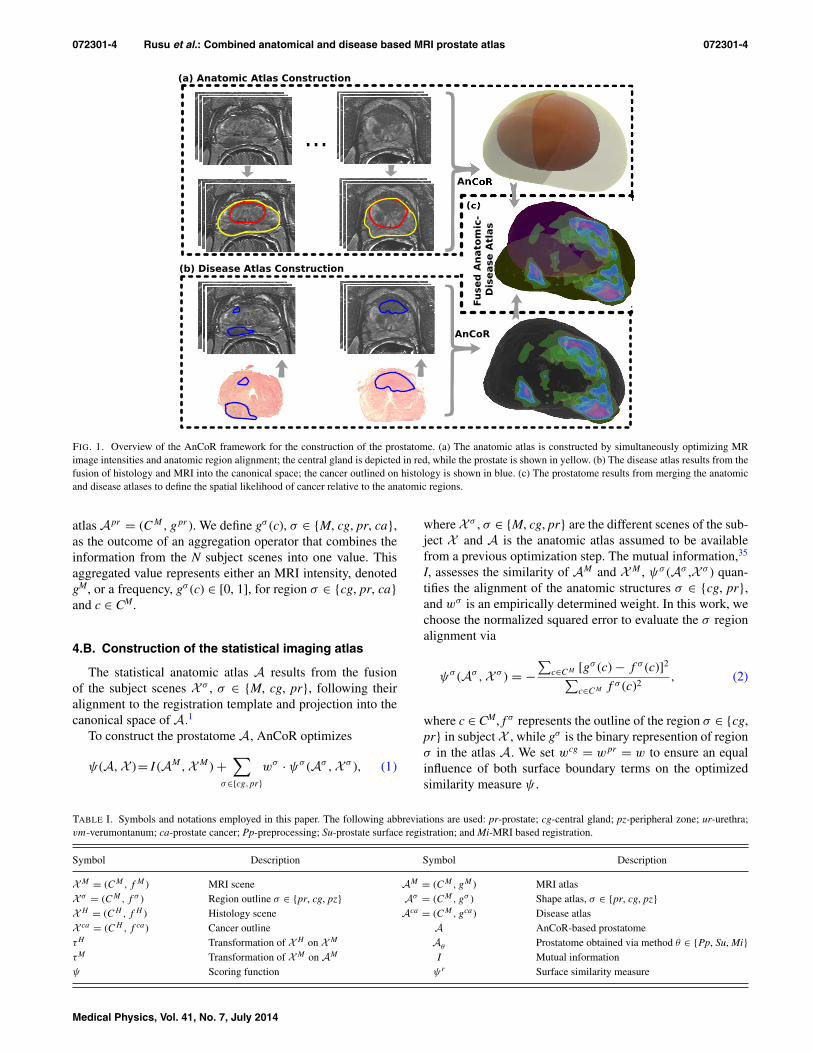
The AnCoR framework allows for the construction of theimaging [Fig. 1(a)] and disease atlases [Fig. 1(b)] and theirfusion into the prostatome [Fig. 1(c)], while simultaneouslyconstraining and ensuring the alignment of different anatomicregions. Such anatomic constraints are incorporated directlyinto the similarity measure, which evaluates both MRI inten-sity as well as the surface misalignment of the central glandand the prostate boundaries. The central gland is assumed toencompass both the central and transitional zones since theirboundaries cannot be readily discerned on T2-w MRI. Sur-rounding the central gland, the peripheral zone occupies therest of the prostate and is implicitly modeled by our frame-work. The central gland and the peripheral zone are anatomi-cally different,33 as can be seen on T2-w MRI,34 where typi-cally peripheral zone appears hyperintense, while the centralgland and tumor reveal a hypointense appearance.

Both imaging and disease atlases are constructed us-ing anatomical constraints placed on the central gland andprostate surface. The AnCoR framework uses an iterative ap-proach that progressively increases the optimized degrees offreedom, from simple translation and scaling to deformabletransformations. At each step, the framework maintains thealignment of the MRI, the subregions, and tumor. This en-sures that only one transformation is needed to project allinformation pertinent to a subject onto the canonical space.

4. METHODOLOGICAL DESCRIPTION

4.A. Notations

The notations used in this paper are summarized in Table I.A study X is defined by (1) an MRI scene XM = (CM, f M ),where CM is the 3D grid and f M(c) represents the MRI in-tensity at each voxel c ∈ CM and (2) a histology scene XH

= (CH, f H ), with f H(d) the hematoxylin and eosin (H andE) information at each pixel d ∈ CH. Several anatomic re-gions are defined relative to the MRI scene: (1) the prostate(pr), X pr = (CM, f pr ) with f pr(c) = 1 within the prostate andzero elsewhere; (2) the central gland (cg), X cg = (CM, f cg),where f cg(c) = 1 within the central gland, and (3) the pe-ripheral zone (pz), X pz = (CM, f pz), with f pz(c) = 1 withinthe peripheral zone. The tumor is delineated by an expertpathologist relative to the histology scene, XH , and definedby X ca = (CH, f ca) where f ca(d) = 1 where the cancer ispresent.

The prostatome A results from the fusion of the diseaseatlas Aca , the MRI intensity atlas, AM = (CM, gM ), the cen-tral gland shape atlas Acg = (CM, gcg), and the prostate shape

Medical Physics, Vol. 41, No. 7, July 2014

072301-4 Rusu et al.: Combined anatomical and disease based MRI prostate atlas 072301-4

FIG. 1. Overview of the AnCoR framework for the construction of the prostatome. (a) The anatomic atlas is constructed by simultaneously optimizing MRimage intensities and anatomic region alignment; the central gland is depicted in red, while the prostate is shown in yellow. (b) The disease atlas results from thefusion of histology and MRI into the canonical space; the cancer outlined on histology is shown in blue. (c) The prostatome results from merging the anatomicand disease atlases to define the spatial likelihood of cancer relative to the anatomic regions.

atlas Apr = (CM, gpr ). We define gσ (c), σ ∈ {M, cg, pr, ca},as the outcome of an aggregation operator that combines theinformation from the N subject scenes into one value. Thisaggregated value represents either an MRI intensity, denotedgM, or a frequency, gσ (c) ∈ [0, 1], for region σ ∈ {cg, pr, ca}and c ∈ CM.

4.B. Construction of the statistical imaging atlas

The statistical anatomic atlas A results from the fusionof the subject scenes X σ , σ ∈ {M, cg, pr}, following theiralignment to the registration template and projection into thecanonical space of A.1

To construct the prostatome A, AnCoR optimizes

ψ(A,X )=I (AM,XM ) +∑

σ∈{cg,pr}wσ · ψσ (Aσ ,X σ ), (1)

where X σ , σ ∈ {M, cg, pr} are the different scenes of the sub-ject X and A is the anatomic atlas assumed to be availablefrom a previous optimization step. The mutual information,35

I, assesses the similarity of AM and XM , ψσ (Aσ ,X σ ) quan-tifies the alignment of the anatomic structures σ ∈ {cg, pr},and wσ is an empirically determined weight. In this work, wechoose the normalized squared error to evaluate the σ regionalignment via

ψσ (Aσ ,X σ ) = −∑

c∈CM [gσ (c) − f σ (c)]2

∑c∈CM f σ (c)2

, (2)

where c ∈ CM, f σ represents the outline of the region σ ∈ {cg,pr} in subject X , while gσ is the binary represention of regionσ in the atlas A. We set wcg = wpr = w to ensure an equalinfluence of both surface boundary terms on the optimizedsimilarity measure ψ .

TABLE I. Symbols and notations employed in this paper. The following abbreviations are used: pr-prostate; cg-central gland; pz-peripheral zone; ur-urethra;vm-verumontanum; ca-prostate cancer; Pp-preprocessing; Su-prostate surface registration; and Mi-MRI based registration.

Symbol Description Symbol Description

XM = (CM, f M ) MRI scene AM = (CM, gM ) MRI atlasX σ = (CM, f σ ) Region outline σ ∈ {pr, cg, pz} Aσ = (CM, gσ ) Shape atlas, σ ∈ {pr, cg, pz}XH = (CH , f H ) Histology scene Aca = (CM, gca) Disease atlasX ca = (CH , f ca) Cancer outline A AnCoR-based prostatomeτH Transformation of XH on XM Aθ Prostatome obtained via method θ ∈ {Pp, Su, Mi}τM Transformation of XM on AM I Mutual informationψ Scoring function ψ r Surface similarity measure

Medical Physics, Vol. 41, No. 7, July 2014

072301-5 Rusu et al.: Combined anatomical and disease based MRI prostate atlas 072301-5

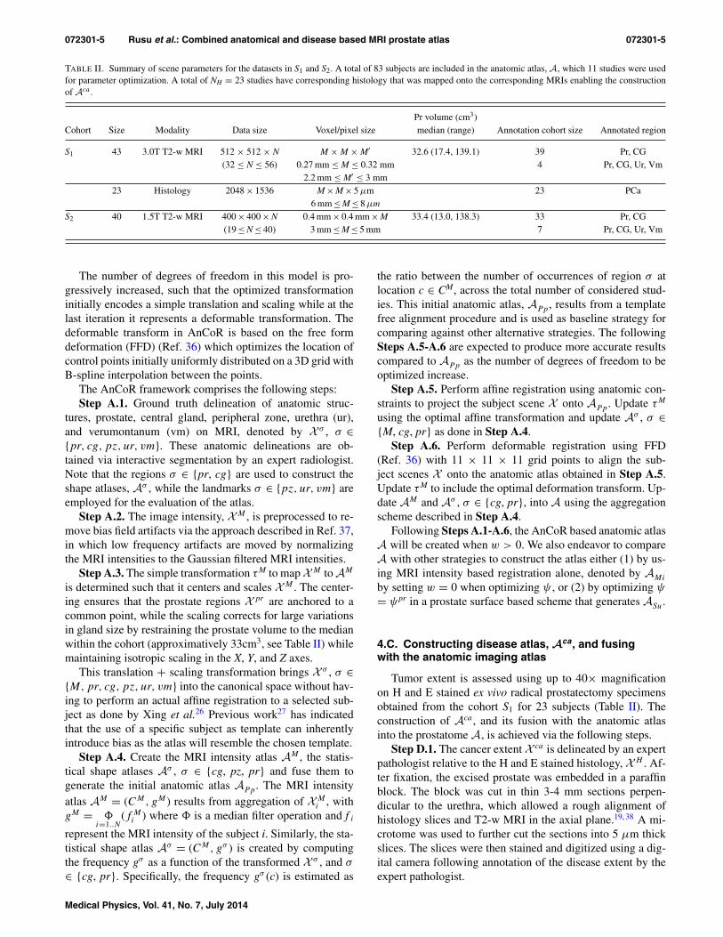
TABLE II. Summary of scene parameters for the datasets in S1 and S2. A total of 83 subjects are included in the anatomic atlas, A, which 11 studies were usedfor parameter optimization. A total of NH = 23 studies have corresponding histology that was mapped onto the corresponding MRIs enabling the constructionof Aca .

Pr volume (cm3)Cohort Size Modality Data size Voxel/pixel size median (range) Annotation cohort size Annotated region

S1 43 3.0T T2-w MRI 512 × 512 × N M × M × M′ 32.6 (17.4, 139.1) 39 Pr, CG(32 ≤ N ≤ 56) 0.27 mm ≤ M ≤ 0.32 mm 4 Pr, CG, Ur, Vm

2.2 mm ≤ M′ ≤ 3 mm23 Histology 2048 × 1536 M × M × 5 μm 23 PCa

6 mm ≤ M ≤ 8 μmS2 40 1.5T T2-w MRI 400 × 400 × N 0.4 mm × 0.4 mm × M 33.4 (13.0, 138.3) 33 Pr, CG

(19 ≤ N ≤ 40) 3 mm ≤ M ≤ 5 mm 7 Pr, CG, Ur, Vm

The number of degrees of freedom in this model is pro-gressively increased, such that the optimized transformationinitially encodes a simple translation and scaling while at thelast iteration it represents a deformable transformation. Thedeformable transform in AnCoR is based on the free formdeformation (FFD) (Ref. 36) which optimizes the location ofcontrol points initially uniformly distributed on a 3D grid withB-spline interpolation between the points.

The AnCoR framework comprises the following steps:Step A.1. Ground truth delineation of anatomic struc-

tures, prostate, central gland, peripheral zone, urethra (ur),and verumontanum (vm) on MRI, denoted by X σ , σ ∈{pr, cg, pz, ur, vm}. These anatomic delineations are ob-tained via interactive segmentation by an expert radiologist.Note that the regions σ ∈ {pr, cg} are used to construct theshape atlases, Aσ , while the landmarks σ ∈ {pz, ur, vm} areemployed for the evaluation of the atlas.

Step A.2. The image intensity, XM , is preprocessed to re-move bias field artifacts via the approach described in Ref. 37,in which low frequency artifacts are moved by normalizingthe MRI intensities to the Gaussian filtered MRI intensities.

Step A.3. The simple transformation τM to map XM to AM

is determined such that it centers and scales XM . The center-ing ensures that the prostate regions X pr are anchored to acommon point, while the scaling corrects for large variationsin gland size by restraining the prostate volume to the medianwithin the cohort (approximatively 33cm3, see Table II) whilemaintaining isotropic scaling in the X, Y, and Z axes.

This translation + scaling transformation brings X σ , σ ∈{M,pr, cg, pz, ur, vm} into the canonical space without hav-ing to perform an actual affine registration to a selected sub-ject as done by Xing et al.26 Previous work27 has indicatedthat the use of a specific subject as template can inherentlyintroduce bias as the atlas will resemble the chosen template.

Step A.4. Create the MRI intensity atlas AM , the statis-tical shape atlases Aσ , σ ∈ {cg, pz, pr} and fuse them togenerate the initial anatomic atlas APp. The MRI intensityatlas AM = (CM, gM ) results from aggregation of XM

i , withgM = �

i=1..N(f M

i ) where � is a median filter operation and f i

represent the MRI intensity of the subject i. Similarly, the sta-tistical shape atlas Aσ = (CM, gσ ) is created by computingthe frequency gσ as a function of the transformed X σ , and σ

∈ {cg, pr}. Specifically, the frequency gσ (c) is estimated as

the ratio between the number of occurrences of region σ atlocation c ∈ CM, across the total number of considered stud-ies. This initial anatomic atlas, APp, results from a templatefree alignment procedure and is used as baseline strategy forcomparing against other alternative strategies. The followingSteps A.5-A.6 are expected to produce more accurate resultscompared to APp as the number of degrees of freedom to beoptimized increase.

Step A.5. Perform affine registration using anatomic con-straints to project the subject scene X onto APp. Update τM

using the optimal affine transformation and update Aσ , σ ∈{M, cg, pr} as done in Step A.4.

Step A.6. Perform deformable registration using FFD(Ref. 36) with 11 × 11 × 11 grid points to align the sub-ject scenes X onto the anatomic atlas obtained in Step A.5.Update τM to include the optimal deformation transform. Up-date AM and Aσ , σ ∈ {cg, pr}, into A using the aggregationscheme described in Step A.4.

Following Steps A.1-A.6, the AnCoR based anatomic atlasA will be created when w > 0. We also endeavor to compareA with other strategies to construct the atlas either (1) by us-ing MRI intensity based registration alone, denoted by AMi

by setting w = 0 when optimizing ψ , or (2) by optimizing ψ

= ψpr in a prostate surface based scheme that generates ASu.

4.C. Constructing disease atlas, Aca, and fusingwith the anatomic imaging atlas

Tumor extent is assessed using up to 40× magnificationon H and E stained ex vivo radical prostatectomy specimensobtained from the cohort S1 for 23 subjects (Table II). Theconstruction of Aca , and its fusion with the anatomic atlasinto the prostatome A, is achieved via the following steps.

Step D.1. The cancer extent X ca is delineated by an expertpathologist relative to the H and E stained histology, XH . Af-ter fixation, the excised prostate was embedded in a paraffinblock. The block was cut in thin 3-4 mm sections perpen-dicular to the urethra, which allowed a rough alignment ofhistology slices and T2-w MRI in the axial plane.19, 38 A mi-crotome was used to further cut the sections into 5 μm thickslices. The slices were then stained and digitized using a dig-ital camera following annotation of the disease extent by theexpert pathologist.

Medical Physics, Vol. 41, No. 7, July 2014

072301-6 Rusu et al.: Combined anatomical and disease based MRI prostate atlas 072301-6

Step D.2. Correspondences between the slices in the his-tology XH and MRI Scenes XM are identified by an expertradiologist and an expert pathologist working in unison. Thisstrategy previously described in details in Refs. 15 and 19 in-volves identifying corresponding anatomic landmarks, e.g.,urethra, verumontanum, or benign prostatic hyperplasia onboth the MRI and histology sections to determine the bestmatch. This correspondence determination is facilitated bythe fact that the histology slices are cut perpendicular to theurethra, in roughly the same orientation as the MR images.

Step D.3. The mapping of tumor extent X ca onto XM

was achieved using the deformable transform τH that warpsXH onto XM obtained via the approach presented by Chap-pelow et al.19 The approach uses a multiattribute combinedmutual information (MACMI) scheme to automatically alignXH onto XM , and subsequently map X ca onto XM .

Step D.4. X ca is projected onto A by applying τM, ob-tained and update iteratively in Steps A.3, A.5.-A.6.

Step D.5. Update Aca by estimating the frequency of can-cer occurrence, gca(c) for ∀c ∈ CM, as a function of the cancerextent f ca

i (c) of each subject Xi , i ∈ {1, . . . , 23} for whichthe cancer was mapped from histology onto MRI. The fre-quency gca(c) is obtained as the ratio between the number ofoccurrences of cancer at location c ∈ CM aggregated for allsubjects Xi , i ∈ {1, . . . , 23} and the total number of subjects(23) with a histologic annotation of cancer presence. Aca isassessed in 3D relative to AM , and when merged with the in-tensity atlas AM and shape atlases Apr and Acg , results in theprostatome A.

5. EXPERIMENTAL RESULTS AND DISCUSSION

5.A. Data description

Table II describes the data used in our study. The imaginganatomic atlas was built based on endorectal T2-w MRI ac-quired from 83 subjects with biopsy confirmed cancer fromtwo institutions. The disease atlas, Aca was constructed fromthe 23 subject subpopulation in cohort S1 for which ex vivohistopathology of the radical prostatectomy was available. S1

was used for mapping extent of cancer onto the correspondingin vivo MRI. Figure 1 shows corresponding MRI for two dif-ferent subjects from S1, for which the central gland, prostate,and tumor are highlighted in red, yellow, and blue, respec-tively.

The 23 patient studies used to construct the disease at-las Aca were chosen from a larger cohort of 124 cases, allof which included an MRI exam prior to radical prostate-ctomy. Of the 124 cases, only 65 studies had usable T2-wMRI with corresponding digitized whole mount histologicalsections. Of those, 43 randomly chosen cases had the centralgland and peripheral zone annotated by an expert radiologistand were included in the cohort S1. Twenty three patient stud-ies in S1 were identified with histological sections on whichCaP was visible and could be annotated by the expert patholo-gist. Forty studies were chosen randomly from a cohort of 83consecutive cases available from a second institution. Thesewere annotated by the expert radiologist and included in S2.

5.B. Evaluation of the imaging atlas

The imaging atlas is evaluated through two performancemeasures, the deviation between the anatomic landmarks σ ∈{ur, vm} and overlap of anatomic regions, σ ∈ {pr, cg, pz}.The measures are estimated based off landmarks and regionsthat are consistently discernible across different subjects in S1

and S2.

5.B.1. Landmark based measures

The anatomic landmarks considered for evaluation are theurethra (ur) and verumontanum (vm). Anatomically, the ure-thra is a tubular curved structure located centrally within theprostate from base to apex while the verumontanum has a v-like shape visible in the midgland region on just a few axialslices. Other landmarks such as benign prostatic hyperplasianodules or calcifications are not consistent discernible acrosssubjects and hence were not considered. The successful reg-istration of the subject scene XM with the prostatome A isexpected to result in the intersubject alignment of the land-marks that are consistently distinguishable between patients.

In order to compute the deviation between the anatomiclandmarks σ ∈ {ur, vm}, their 3D medial axis39 was firstcomputed and then the deviation between the points on themedial axis was estimated. The medial axis is defined in 3D asthe points at the interior of the region σ that are furthest awayfrom the annotated surface. For two subjects Xi and Xj weestimated the medial axis deviation denoted by ||X σ

i ,X σj ||m

as to the average Euclidean distance between proximal pointson their respective medial axes.

The point cip on the medial axis of subject Xi is consideredproximal to cjq on the medial axis of subject Xj if ||cip, cjq||2≤ ||cip, cjr||2, where cjr is any point on the medial axis ofsubject Xj , such that r �= q. Note that if cip is proximal tocjq this does not imply that cjq is proximal to cip. Thus, weestimate the average deviation between anatomic landmarksof subject X σ

i and X σj as

∣∣∣∣X σi,j

∣∣∣∣m

= 1

2· (∣∣∣∣X σ

i ,X σj

∣∣∣∣m

+ ∣∣∣∣X σj ,X σ

i

∣∣∣∣m

), (3)

where σ ∈ {ur, vm}.The average deviation of the landmarks within the evalua-

tion cohort (Nev = 11 studies from cohorts S1 and S2) is deter-mined as the averaged intersubject deviations for any possiblepair-wise combination of subjects. For Nev subject scenes X σ

i ,∀i ∈ {1, . . . , Nev}, ||X σ

1,...,Nev||m is defined for σ ∈ {ur, vm}

as

∣∣∣∣X σ1,...,Nev

∣∣∣∣m

= 2

Nev(Nev − 1)·

Nev−1∑

i=1

Nev∑

j=i+1

∣∣∣∣Xσi,j

∣∣∣∣m. (4)

5.B.2. Region based measures

The Dice similarity coefficient (DSC) represents the over-lap between two regions X σ

i and X σj :

DSC(X σ

i ,X σj

) = 2 × ∣∣X σi

⋂X σ

j

∣∣∣∣X σ

i

∣∣ + ∣∣X σj

∣∣ , (5)

Medical Physics, Vol. 41, No. 7, July 2014

072301-7 Rusu et al.: Combined anatomical and disease based MRI prostate atlas 072301-7

(a) (b) (c) (d)

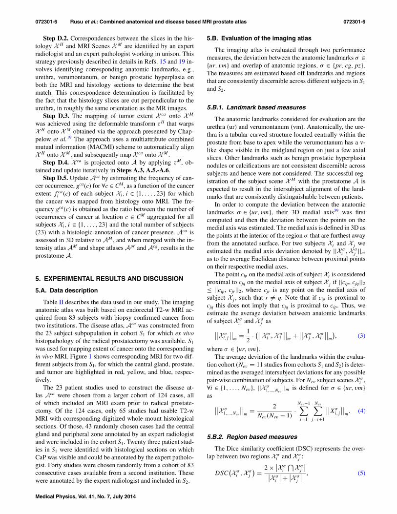
FIG. 2. Trend of performance evaluation measures and errors estimated for A as a function of w (a) prostate DSC, (b) central gland DSC, misalignment errorof the (c) urethra, and (d) verumontanum. Higher DSC and lower misalignment errors are desirable. Error bars are used to indicate the standard deviation of themeasure.

where |X σ | represents the number of voxels in region σ ∈{cg, pr}.

To estimate the population overlap of anatomic regions σ

∈ {cg, pr}, we compute the averaged DSC as

DSC(X σ

1,...,N

) = 1

N

N∑

i=1

DSC(X σ

i ,Aσ), (6)

where Aσ represents the binary form of the shape atlas withσ ∈ {pr, cg, pz}.

The atlas construction framework was implemented usingthe ITK framework.40

5.C. Parameter optimization

In order to identify the optimal contribution of theanatomic constraints, defined by the weight w, the prosta-teome A was constructed using Nev = 11 studies selectedfrom the two cohorts S1 and S2 (Table II). For w ∈ [0, 1],with a step size of 0.05-0.1, we evaluate the landmarkdeviation, ||X σ

1,...,Nev||m, σ ∈ {ur, vm}, and region overlap,

DSC(X σ1,...,Nev

), σ ∈ {cg, pr, pz}, obtained when construct-ing the anatomic atlas A in the affine (Step A.5.) and de-formable (Step A.6.) registration steps, respectively.

Our results suggest that w > 1.0 did not yield significantchanges in landmark misalignment or region overlap. Thisis probably because increasing w transforms the registrationinto a surface based alignment scheme with essentially nocontribution from the intensity term, I.

In the affine registration step (Fig. 2), both ||X σ1,...,Nev

||m,

σ ∈ {ur, vm} and DSC(X σ1,...,Nev

), σ ∈ {cg, pr, pz} improvedfor w > 0 when compared to the baseline w = 0, which isequivalent to AMi . These results indicate the need of sur-face constraints as defined in the AnCoR framework for ac-curate prostatome construction. However, for w > 0.5, thecentral gland or prostate DSC and landmark misalignment er-ror remain relatively constant, indicating that the influencesof the surface terms significantly outweigh the influence ofthe intensity term. Therefore since w = 0.5 yielded the high-est DSC(X σ

1,...,Nev) with minimal ||X σ

1,...,Nev||m, we choose this

value for constructing A.When evaluating A after deformable registration, trends

in DSC were observed to be similar to the affine registra-tion step (Fig. 2). DSC(X σ

1,...,Nev) increases progressively up

to w = 0.2, beyond which, it converges to a region overlapvalue of 93%. This value is higher than observed in the affineregistration step which suggests the need of the deformableregistration step when constructing A. The landmark mis-alignment is roughly constant for values of w < 0.1, but fluc-tuates as w increases. The value of w was set equal to 0.05 inthe deformable registration step based on an optimal trade-offbetween ||X σ

1,...,Nev||m and DSC(X σ

1,...,Nev).

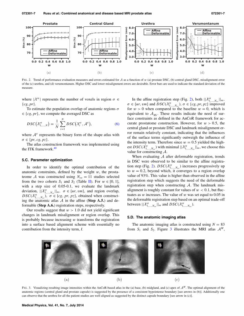
5.D. The anatomic imaging atlas

The anatomic imaging atlas is constructed using N = 83from S1 and S2. Figure 3 illustrates the MRI atlas AM ,

(a) (b) (c)

FIG. 3. Visualizing resulting image intensities within the AnCoR-based atlas in the (a) base, (b) midgland, and (c) apex of AM . The optimal alignment of theanatomic regions (central gland and prostate capsule) is suggested by the presence of a consistent hypointense boundary [see arrows in (b)]. Additionally onecan observe that the urethra for all the patient studies are well aligned as suggested by the distinct capsule boundary [see arrow in (c)].

Medical Physics, Vol. 41, No. 7, July 2014

072301-8 Rusu et al.: Combined anatomical and disease based MRI prostate atlas 072301-8

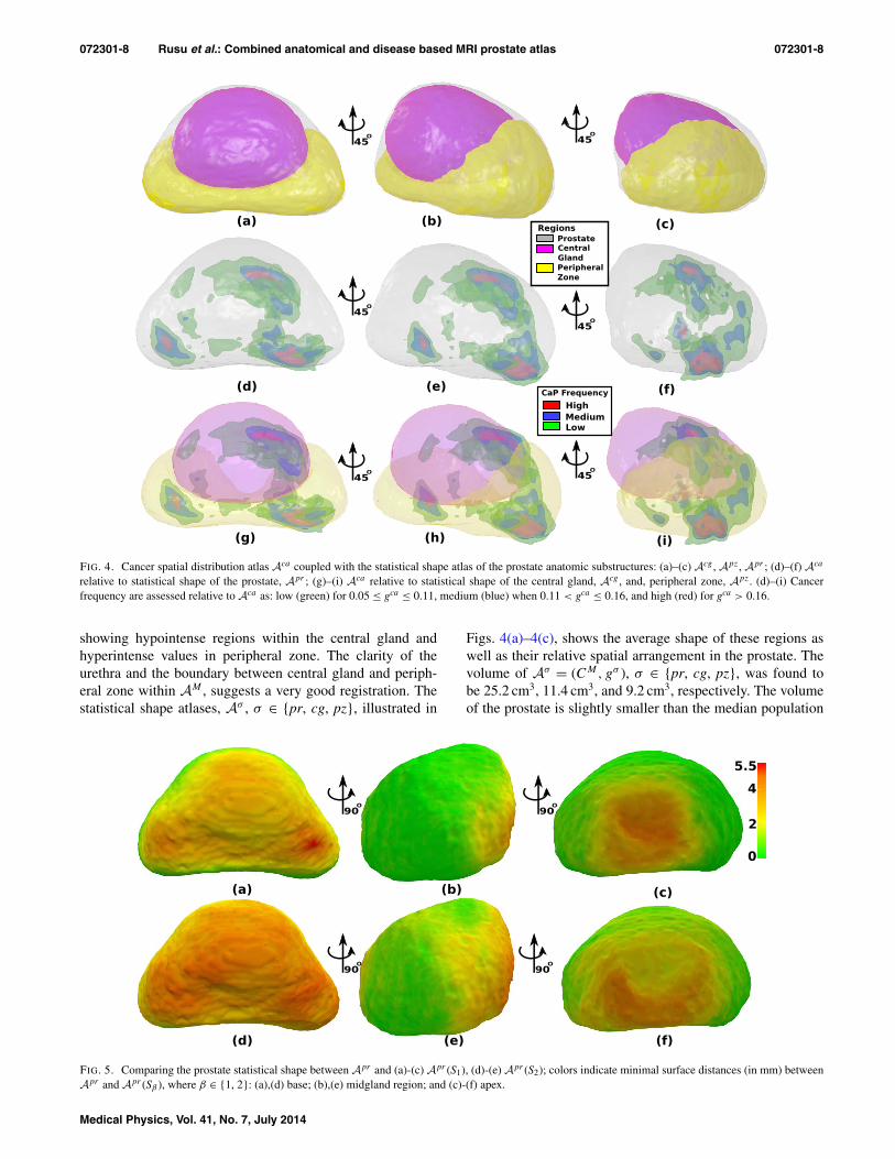
FIG. 4. Cancer spatial distribution atlas Aca coupled with the statistical shape atlas of the prostate anatomic substructures: (a)–(c) Acg , Apz, Apr ; (d)–(f) Aca

relative to statistical shape of the prostate, Apr ; (g)–(i) Aca relative to statistical shape of the central gland, Acg , and, peripheral zone, Apz. (d)–(i) Cancerfrequency are assessed relative to Aca as: low (green) for 0.05 ≤ gca ≤ 0.11, medium (blue) when 0.11 < gca ≤ 0.16, and high (red) for gca > 0.16.

showing hypointense regions within the central gland andhyperintense values in peripheral zone. The clarity of theurethra and the boundary between central gland and periph-eral zone within AM , suggests a very good registration. Thestatistical shape atlases, Aσ , σ ∈ {pr, cg, pz}, illustrated in

Figs. 4(a)–4(c), shows the average shape of these regions aswell as their relative spatial arrangement in the prostate. Thevolume of Aσ = (CM, gσ ), σ ∈ {pr, cg, pz}, was found tobe 25.2 cm3, 11.4 cm3, and 9.2 cm3, respectively. The volumeof the prostate is slightly smaller than the median population

FIG. 5. Comparing the prostate statistical shape between Apr and (a)-(c) Apr (S1), (d)-(e) Apr (S2); colors indicate minimal surface distances (in mm) betweenApr and Apr (Sβ ), where β ∈ {1, 2}: (a),(d) base; (b),(e) midgland region; and (c)-(f) apex.

Medical Physics, Vol. 41, No. 7, July 2014

072301-9 Rusu et al.: Combined anatomical and disease based MRI prostate atlas 072301-9

TABLE III. Prostate, central gland DSC, and landmark misalignment evalu-ated when computing the anatomic atlas across sites A or within sites, A(S1)and A(S2). Cohort S1 seems to have a more homogeneous population com-pared to cohort S2, as reflected via the DSC and minimal landmark misalign-ment measures.

Pr DSC CG DSC Ur Dev Vm DevAtlas Cohort (%) (%) (mm) (mm)

A S1;S2 88 90 3.45 4.73A(S1) S1 92 90 2.57 2.82A(S2) S2 89 89 3.76 4.51

volume, on account of shrinkage caused by preprocessing stepand the affine registration.

5.E. The disease atlas, Aca

Figure 4 illustrates the spatial distribution of cancerwithin Apr [Figs. 4(d)–4(f)] as well as within Acg and Apz

[Figs. 4(g)–4(i)]. As previously suggested,41 the highest fre-quency of cancer is present in the peripheral zone proximal tothe neurovascular bundles. However, preponderance of canceris also observed in the central gland toward the prostate apex.Central gland tumors were observed to be larger in volume

which renders them more likely to spatially overlap withinthe atlas, thus resulting in a visibly higher spatial frequencywithin the central gland. Although atypical, such findings areconsistent with the fact that central gland tumors are oftendetected at later stages of disease, and thus are considerablylarger in volume than the peripheral zone tumors. Addition-ally, the spatial distribution of tumor was not symmetric asindicated previously.42

5.F. Comparing atlas appearance across sites

To evaluate the precise variability in the appearance of theimaging atlases constructed using data from the two sites,we constructed A using data from (1) cohort S1 alone (43subjects) and referred to as A(S1), (2) cohort S2 alone (40subjects) and referred to as A(S2) and (3) cohorts S1 and S2

together (83 subjects) referred to as A (Fig. 5). Although theprostate median volume was consistent across the two sites(Table II), the statistical shape of the anatomic regions differs,particularly in the base and apex regions. Figure 5 shows thesurface distances between the Apr compared to the prostateshape in Apr (S1) and Apr (S2). Near perfect alignment isobservable in the midgland [Figs. 5(b) and 5(e)], while up to5 mm misalignment error is observable in the base and apex.

(a)AMi (b)ASu (c)A

(d)AMi (e)ASu (f)A

(g)AMi (h)ASu (i)A

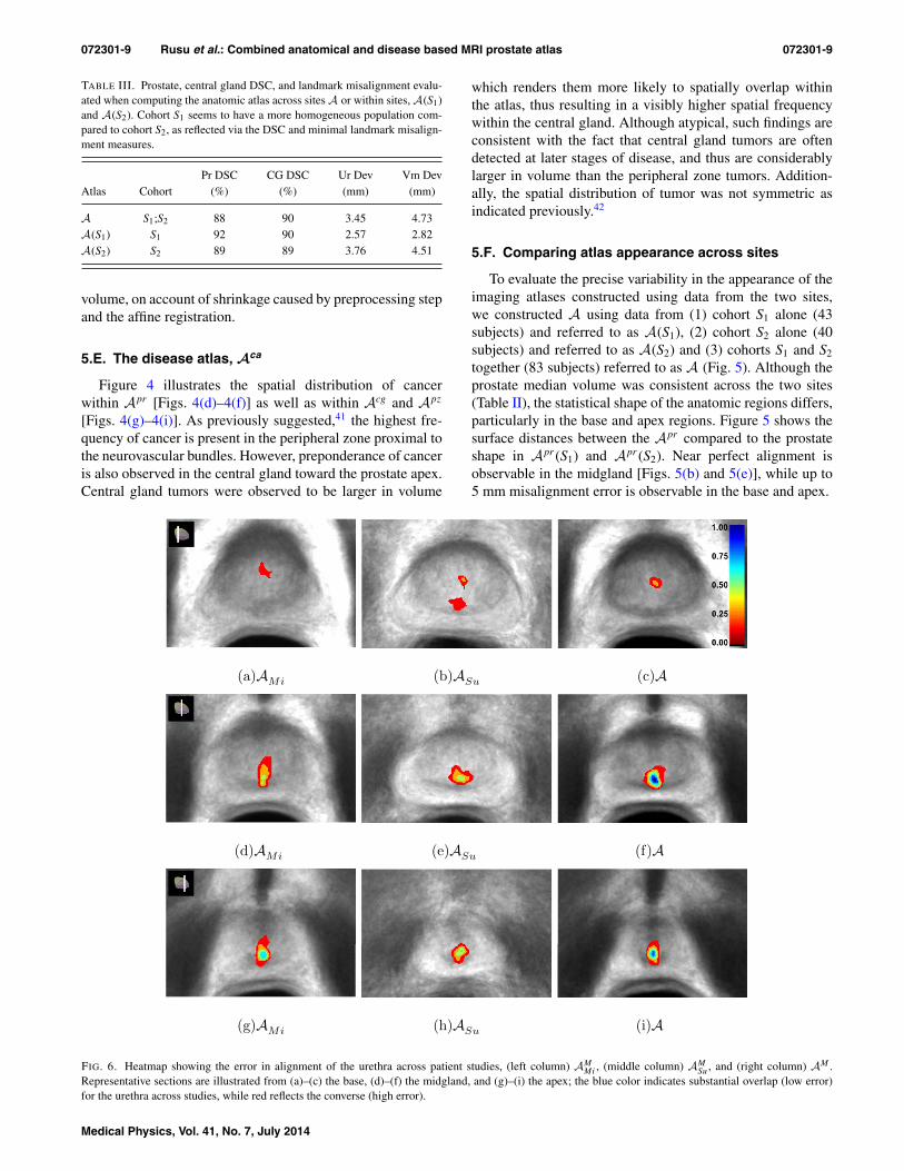
FIG. 6. Heatmap showing the error in alignment of the urethra across patient studies, (left column) AMMi , (middle column) AM

Su, and (right column) AM .Representative sections are illustrated from (a)–(c) the base, (d)–(f) the midgland, and (g)–(i) the apex; the blue color indicates substantial overlap (low error)for the urethra across studies, while red reflects the converse (high error).

Medical Physics, Vol. 41, No. 7, July 2014

072301-10 Rusu et al.: Combined anatomical and disease based MRI prostate atlas 072301-10

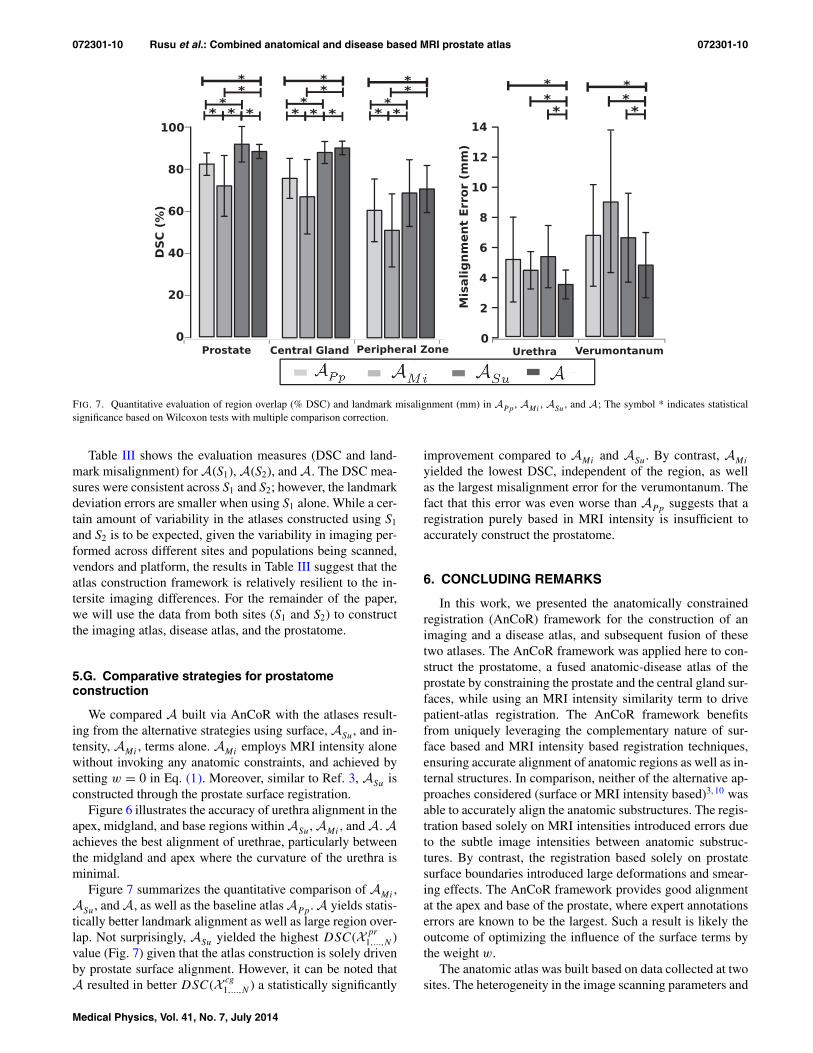
FIG. 7. Quantitative evaluation of region overlap (% DSC) and landmark misalignment (mm) in APp , AMi , ASu, and A; The symbol * indicates statisticalsignificance based on Wilcoxon tests with multiple comparison correction.

Table III shows the evaluation measures (DSC and land-mark misalignment) for A(S1), A(S2), and A. The DSC mea-sures were consistent across S1 and S2; however, the landmarkdeviation errors are smaller when using S1 alone. While a cer-tain amount of variability in the atlases constructed using S1

and S2 is to be expected, given the variability in imaging per-formed across different sites and populations being scanned,vendors and platform, the results in Table III suggest that theatlas construction framework is relatively resilient to the in-tersite imaging differences. For the remainder of the paper,we will use the data from both sites (S1 and S2) to constructthe imaging atlas, disease atlas, and the prostatome.

5.G. Comparative strategies for prostatomeconstruction

We compared A built via AnCoR with the atlases result-ing from the alternative strategies using surface, ASu, and in-tensity, AMi , terms alone. AMi employs MRI intensity alonewithout invoking any anatomic constraints, and achieved bysetting w = 0 in Eq. (1). Moreover, similar to Ref. 3, ASu isconstructed through the prostate surface registration.

Figure 6 illustrates the accuracy of urethra alignment in theapex, midgland, and base regions within ASu, AMi , and A. Aachieves the best alignment of urethrae, particularly betweenthe midgland and apex where the curvature of the urethra isminimal.

Figure 7 summarizes the quantitative comparison of AMi ,ASu, and A, as well as the baseline atlas APp. A yields statis-tically better landmark alignment as well as large region over-lap. Not surprisingly, ASu yielded the highest DSC(X pr

1,...,N )value (Fig. 7) given that the atlas construction is solely drivenby prostate surface alignment. However, it can be noted thatA resulted in better DSC(X cg

1,...,N ) a statistically significantly

improvement compared to AMi and ASu. By contrast, AMi

yielded the lowest DSC, independent of the region, as wellas the largest misalignment error for the verumontanum. Thefact that this error was even worse than APp suggests that aregistration purely based in MRI intensity is insufficient toaccurately construct the prostatome.

6. CONCLUDING REMARKS

In this work, we presented the anatomically constrainedregistration (AnCoR) framework for the construction of animaging and a disease atlas, and subsequent fusion of thesetwo atlases. The AnCoR framework was applied here to con-struct the prostatome, a fused anatomic-disease atlas of theprostate by constraining the prostate and the central gland sur-faces, while using an MRI intensity similarity term to drivepatient-atlas registration. The AnCoR framework benefitsfrom uniquely leveraging the complementary nature of sur-face based and MRI intensity based registration techniques,ensuring accurate alignment of anatomic regions as well as in-ternal structures. In comparison, neither of the alternative ap-proaches considered (surface or MRI intensity based)3, 10 wasable to accurately align the anatomic substructures. The regis-tration based solely on MRI intensities introduced errors dueto the subtle image intensities between anatomic substruc-tures. By contrast, the registration based solely on prostatesurface boundaries introduced large deformations and smear-ing effects. The AnCoR framework provides good alignmentat the apex and base of the prostate, where expert annotationserrors are known to be the largest. Such a result is likely theoutcome of optimizing the influence of the surface terms bythe weight w.

The anatomic atlas was built based on data collected at twosites. The heterogeneity in the image scanning parameters and

Medical Physics, Vol. 41, No. 7, July 2014

072301-11 Rusu et al.: Combined anatomical and disease based MRI prostate atlas 072301-11

population is reflected most prominently in the base and apexof the prostatome. Future work will attempt to capture thevariability in MRI intensity between sites.

Through the fusion of in vivo MRI and histology withprostate cancer delineation, we were able to create a diseaseatlas which allowed us to estimate the 3D spatial distribu-tion of cancer relative to the anatomic substructures of theprostate. While our studies comprised a larger number of pe-ripheral zone tumors, the central gland tumors tended to belarger in size. To our knowledge this is the first study attempt-ing to estimate the prostate cancer distribution in 3D relativeto the anatomic structures of the prostate via in vivo MRI. Thesmall cohort of 23 patient for which cancer ground truth wasavailable in this study, allowed us to create a preliminary ver-sion of the prostatome. With inclusion of additional studiesin the future, we seek to increase the statistical power of theprostatome. We anticipate that the atlas could serve as a guidefor directed biopsies and targeted treatment. Of potential clin-ical impact as well, is the use of this approach for surgicalor radiotherapy planning intended to spare the anatomicallyclosely adjacent neurovascular bundles so as to reduce the in-cidence of unintended impotence.

We acknowledge that our study had a few limitations. Ourapproach used manual delineation of the anatomic regions,the central gland, peripheral zone, and prostate. As we lookto increase the number of studies to be incorporated intoprostatome, clearly manual delineation will be unfeasible andalso subject to inter- and intraobserver variability. Toward thisend our group has already developed automated schemes forsegmentation of substructures within the prostate.43, 44 TheAnCoR framework is designed to allow the simultaneous op-timization of MR image intensity similarity and anatomic re-gion overlap without explicitly reinforcing the preservationof region volume. The choice of template and the simultane-ous consideration of both central gland and prostate regionin the optimization will affect the volume of the prostate fol-lowing registration. The possible changes in prostate volumeafter registration does not however influence the ability of theframework to create a unified canonical representation of thepatient cohort to study the spatial distribution of cancer. Fi-nally, our elastic registration step uses free form deformation(FFD).36 We will look to integrate smoothness and additionalregularization within FFD as part of future work.

Despite these limitations, our AnCoR framework providesa platform for the fusion of multimodal data into a singlecanonical representation. The prostatome could ultimatelypave the way for the study of in vivo imaging markers associ-ated with aggressive disease. Moreover, this framework couldserve as a model for the integration of multimodal, multiscaleimaging and molecular data which could pave the way for cre-ation of a fused imaging-pathology-omics atlas for cross-scaleinterrogation of disease. This could enable correlative studiesof imaging and omics features associated with the disease.

ACKNOWLEDGMENTS

Research reported in this publication was supported by theNational Cancer Institute of the National Institutes of Health

under award numbers R01CA136535-01, R01CA140772-01,and R21CA167811-01; the DOD Prostate Cancer Synergis-tic Idea Development Award (PC120857); the Ohio ThirdFrontier Technology development Grant; the QED awardfrom the University City Science Center, Rutgers Univer-sity and the Department of Defense, Prostate Cancer Post-doctoral Training (W81XWH-12-PCRP-PTA). The content issolely the responsibility of the authors and does not neces-sarily represent the official views of the National Institutes ofHealth.

a)Electronic mail: anant.madabhushi@case.edu1A. C. Evans, D. L. Collins, S. R. Mills, E. D. Brown, R. L. Kelly, andT. M. Peters, “3D statistical neuroanatomical models from 305 MRI vol-umes,” in Nuclear Science Symposium and Medical Imaging Conference(IEEE, San Francisco, CA, 1993), pp. 1813–1817.

2A. W. Toga, P. M. Thompson, S. Mori, K. Amunts, and K. Zilles, “Towardsmultimodal atlases of the human brain,” Nat. Rev. Neurosci. 7, 952–966(2006).

3D. Shen, Z. Lao, J. Zeng, W. Zhang, I. A. Sesterhenn, L. Sun, J. W. Moul,E. H. Herskovits, G. Fichtinger, and C. Davatzikos, “Optimized prostatebiopsy via a statistical atlas of cancer spatial distribution,” Med. ImageAnal. 8, 139–150 (2004).

4Y. Zhan, D. Shen, J. Zeng, L. Sun, G. Fichtinger, J. Moul, and C. Da-vatzikos, “Targeted prostate biopsy using statistical image analysis,” IEEETrans. Pattern Anal. Mach. Intell. 26, 779–788 (2007).

5R. Narayanan, P. N. Werahera, A. Barqawi, E. D. Crawford, K. Shinohara,A. R. Simoneau, and J. S. Suri, “Adaptation of a 3D prostate cancer atlasfor transrectal ultrasound guided target-specific biopsy,” Phys. Med. Biol.53, N397–N406 (2008).

6S. E. Viswanath, N. B. Bloch, J. C. Chappelow, R. Toth, N. M. Rofsky,E. M. Genega, R. E. Lenkinski, and A. Madabhushi, “Central gland and pe-ripheral zone prostate tumors have significantly different quantitative imag-ing signatures on 3 Tesla endorectal, in vivo T2-weighted MR imagery,” J.Magn. Reson. Imaging 36, 213–224 (2012).

7P. Tiwari, J. Kurhanewicz, and A. Madabhushi, “Multi-kernel graph em-bedding for detection, Gleason grading of prostate cancer via MRI/MRS,”Med. Image Anal. 17, 219–235 (2013).

8A. A. Young and A. F. Frangi, “Computational cardiac atlases: From patientto population and back,” Exp. Physiol. 94, 578–596 (2009).

9C. Hoogendoorn, N. Duchateau, D. Sánchez-Quintana, T. Whitmarsh,F. Sukno, M. De Craene, K. Lekadir, and A. F. Frangi, “A high-resolutionatlas and statistical model of the human heart from multislice CT,” IEEETrans. Pattern Anal. Mach. Intell. 32, 28–44 (2013).

10N. Betrouni, A. Iancu, P. Puech, S. Mordon, and N. Makni, “ProstAtlas: Adigital morphologic atlas of the prostate,” Eur. J. Radiol. 81, 3–9 (2011).

11J. Yelnik, E. Bardinet, D. Dormont, G. Malandain, S. Ourselin, D. Tande,C. Karachi, N. Ayache, P. Cornu, and Y. Agid, “A three-dimensional, his-tological and deformable atlas of the human basal ganglia. I. Atlas con-struction based on immunohistochemical and MRI data,” NeuroImage 34,618–638 (2007).

12N. Kovacevic, J. T. Henderson, E. Chan, N. Lifshitz, J. Bishop, A. C. Evans,R. M. Henkelman, and X. J. Chen, “A three-dimensional MRI atlas of themouse brain with estimates of the average and variability,” Cereb. Cortex15, 639–645 (2005).

13K. S. Saleem and N. K. Logothetis, A Combined MRI and Histology Atlasof the Rhesus Monkey Brain in Stereotaxic Coordinates (Academic Press,2012).

14A. Sofer, J. Zeng, and S. K. Mun, “Optimal biopsy protocols for prostatecancer,” Ann. Oper. Res. 119, 63–74 (2003).

15G. Xiao, B. N. Bloch, J. Chappelow, E. Genega, N. Rofsky, R. Lenkin-ski, and A. Madabhushi, “A structural-functional MRI-based disease atlas:Application to computer-aided-diagnosis of prostate cancer,” Proc. SPIE7623, 762303-1–762303-12 (2010).

16M. J. Chelsky, M. D. Schnall, E. J. Seidmon, and H. M. Pollack, “Useof endorectal surface coil magnetic resonance imaging for local staging ofprostate cancer,” J. Urol. 150, 391–395 (1993).

17G. J. Jager, E. T. Ruijter, C. A. van de Kaa, J. J. de la Rosette, G. O. Oost-erhof, J. R. Thornbury, and J. O. Barentsz, “Local staging of prostate

Medical Physics, Vol. 41, No. 7, July 2014

072301-12 Rusu et al.: Combined anatomical and disease based MRI prostate atlas 072301-12

cancer with endorectal MR imaging: Correlation with histopathology,”Am. J. Roentgenol. 166, 845–852 (1996).

18K. K. Yu and H. Hricak, “Imaging prostate cancer,” Radiol. Clin. North.Am. 38, 59–85 (2000).

19J. Chappelow, B. N. Bloch, N. Rofsky, E. Genega, R. Lenkinski, W. De-Wolf, and A. Madabhushi, “Elastic registration of multimodal prostate MRIand histology via multiattribute combined mutual information,” Med. Phys.38, 2005–2018 (2011).

20M. Lorenzo-Valdés, G. I. Sanchez-Ortiz, A. G. Elkington, R. H. Mohi-addin, and D. Rueckert, “Segmentation of 4D cardiac MR images usinga probabilistic atlas and the EM algorithm,” Med. Image Anal. 8, 255–265(2004).

21T. Okada, R. Shimada, Y. Sato, M. Hori, K. Yokota, M. Nakamoto, Y.-W. Chen, H. Nakamura, and S. Tamura, “Automated segmentation of theliver from 3D CT images using probabilistic atlas and multi-level statisticalshape model,” in MICCAI (Springer, Brisbane, Australia, 2007), pp. 86–93.

22S. Klein, U. A. van der Heide, I. M. Lips, M. van Vulpen, M. Staring,and J. P. W. Pluim, “Automatic segmentation of the prostate in 3D MRimages by atlas matching using localized mutual information,” Med. Phys.35, 1407–1417 (2008).

23S. Martin, J. Troccaz, and V. Daanen, “Automated segmentation of theprostate in 3D MR images using a probabilistic atlas and a spatially con-strained deformable model,” Med. Phys. 37, 1579–1590 (2010).

24M. Cabezas, A. Oliver, X. Lladó, J. Freixenet, and M. B. Cuadra, “A re-view of atlas-based segmentation for magnetic resonance brain images,”Comput. Methods Programs Biomed. 104, e158–e177 (2011).

25G. Litjens, O. Debats, W. van de Ven, N. Karssemeijer, and H. Huisman,“A pattern recognition approach to zonal segmentation of the prostate onMRI,” in MICCAI (Springer, Nice, France, 2012), pp. 413–420.

26W. Xing, C. Nan, Z. ZhenTao, X. Rong, J. Luo, Y. Zhuo, S. DingGang, andL. KunCheng, “Probabilistic MRI brain anatomical atlases based on 1,000Chinese subjects,” PLOS One 8, e50939-1–e50939-6 (2013).

27S. Joshi, B. Davis, M. Jomier, and G. Gerig, “Unbiased diffeomorphic atlasconstruction for computational anatomy,” NeuroImage 23(Suppl 1), S151–S160 (2004).

28A. Guimond, J. Meunier, and J.-P. Thirion, “Average brain models: A con-vergence study,” Comput. Vis. Image Und. 77, 192–210 (2000).

29G. E. Christensen, H. J. Johnson, and M. W. Vannier, “Synthesizing average3D anatomical shapes,” NeuroImage 32, 146–158 (2006).

30K. K. Bhatia, J. V. Hajnal, B. K. Puri, A. D. Edwards, and D. Rueck-ert, “Consistent groupwise non-rigid registration for atlas construction,” inIEEE International Symposium on Biomedical Imaging (IEEE, Arlington,VA, 2004), pp. 908–911.

31F. Shi, L. Wang, G. Wu, Y. Zhang, M. Liu, J. H. Gilmore, W. Lin, andD. Shen, “Atlas construction via dictionary learning and group sparsity,”in MICCAI (Springer, Nice, France, 2012), pp. 247–255.

32M. Rusu, B. N. Bloch, C. C. Jaffe, N. Rofsky, E. Genega, R. Lenkinski,and A. Madabhushi, “Statistical 3D prostate imaging atlas constructionvia anatomically constrained registration,” Proc. SPIE 8669, 866913-1–866913-9 (2013).

33J. E. McNeal, “Normal histology of the prostate,” Am. J. Surg. Pathol. 12,619–633 (1988).

34G. M. Villeirs and G. O. De Meerleer, “Magnetic resonance imaging (MRI)anatomy of the prostate and application of MRI in radiotherapy planning,”Eur. J. Radiol. 63, 361–368 (2007).

35J. P. W. Pluim, J. B. A. Maintz, and M. A. Viergever, “Mutual-information-based registration of medical images: A survey,” IEEE Trans. Pattern Anal.Mach. Intell. 22, 986–1004 (2003).

36S. Lee, G. Wolberg, and S. Y. Shin, “Scattered data interpolation with mul-tilevel B-splines,” IEEE Trans. Vis. Comput. Graph. 3, 228–244 (1997).

37M. S. Cohen, R. M. DuBois, and M. M. Zeineh, “Rapid and effective cor-rection of RF inhomogeneity for high field magnetic resonance imaging,”Hum. Brain Mapp. 10, 204–211 (2000).

38G. Xiao, B. N. Bloch, J. Chappelow, E. M. Genega, N. M. Rofsky,R. E. Lenkinski, J. Tomaszewski, M. D. Feldman, M. Rosen, and A. Mad-abhushi, “Determining histology-MRI slice correspondences for definingMRI-based disease signatures of prostate cancer,” Comput. Med. ImagingGraph. 35, 658–578 (2011).

39H. Blum, “A transformation for extracting new descriptors of shape,” inModels for the Perception of Speech and Visual Form (M.I.T. Press, Boston,MA, 1967), pp. 362–380.

40T. S. Yoo, M. J. Ackerman, W. E. Lorensen, W. Schroeder, V. Chalana,S. Aylward, D. Metaxas, and R. Whitaker, “Engineering and algorithm de-sign for an image processing API: A technical report on ITK–the InsightToolkit,” Stud. Health Technol. Inform. 85, 586–92 (2002).

41J. J. Fütterer and J. O. Barentsz, “3T MRI of prostate cancer,” Appl. Radiol.38, 25–32 (2009).

42R. E. Donohue and G. J. Miller, “Adenocarcinoma of the prostate: Biopsyto whole mount. Denver VA experience,” Urol. Clin. North Am. 18, 449–452 (1991).

43R. Toth and A. Madabhushi, “Multifeature landmark-free active appearancemodels: Application to prostate MRI segmentation,” IEEE Trans. PatternAnal. Mach. Intell. 31, 1638–1650 (2012).

44R. Toth, J. Ribault, J. Gentile, D. Sperling, and A. Madabhushi, “Simul-taneous segmentation of prostatic zones using active appearance modelswith multiple coupled levelsets,” Comput. Vis. Image Und. 117, 1051–1060 (2013).

Medical Physics, Vol. 41, No. 7, July 2014