PROTECTED AREA MANAGEMENT IN THE WATERSHED CONTEXT: A CASE

STUDY OF PALO VERDE NATIONAL PARK, COSTA RICA

By

AMY E. DANIELS

A THESIS PRESENTED TO THE GRADUATE SCHOOL OF THE UNIVERSITY OF FLORIDA IN PARTIAL FULFILLMENT

OF THE REQUIREMENTS FOR THE DEGREE OF MASTER OF SCIENCE

UNIVERSITY OF FLORIDA

2004

Copyright 2004

by

Amy E. Daniels

To my mother, Sharon Carlson, whose quiet strength floats me like a river, to the rest of

my family; and to Paul Ghiotto, who held my hand all the way there and back.

ACKNOWLEDGMENTS

I would like to thank my advisor, Hugh Popenoe, whose vast experience around the

globe and understanding of the role of people in shaping the earth—and vice versa—will

forever inspire me. Working with Dr. Popenoe has significantly changed much of my

understanding of resource management, and this thesis was merely the stage on which

that dialogue took place. I am especially grateful for my committee members Graeme

Cumming and Jane Southworth, who supported me in hammering out the nuts and bolts

of this research from concept to the final write-up. Graeme Cumming was always full of

ideas and new approaches for analyzing data. Jane Southworth always offered both

emotional and academic support, along with great practical and technical advice. Her

positive attitude and solutions-oriented approach helped me work through many

methodological challenges to see the light at the end of the tunnel.

Special thanks go to the Organization for Tropical Studies (OTS) in Costa Rica, for

logistical support and for sharing spatial data with me. Eugenio Gonzalez was a great

source of information on everything from driving directions to connections with various

government ministries. He was always supportive in allowing me to participate in

OTS-sponsored activities tangentially related to watershed management. Gary Hartshorn

gave me leads on historical resource management (particularly tree plantations) within

the Tempisque Watershed. I am eternally grateful for the help of Mauricio Castillo, Jose

Antonio Guzman, and Antonio Trabuco who got me through certain GIS and remote

sensing issues in the field. Finally, thanks go to Manuel Blázquez for teaching me about

iv

agricultural practices and irrigation management within the Tempisque Basin. He was

patient during our first conversations when I only understood about half of the Spanish I

heard!

Thanks go to Pete Waylen for sharing precipitation data with me. I would like to

thank the University of Florida’s (UF’s) Land Use and Environmental Change Institute

(LUECI) for giving me generous office space and computer resources for countless hours

of fun-filled image processing and number crunching. I would like to thank my LUECI

office mates, especially Meredith Evans, Andres Guhl, Claudia Stickler, and Zulma

Villega, for their encouragement and consideration throughout the processing and writing

phases. Andres Guhl and Claudia Stickler were always willing to bounce ideas around

with me whenever I got stuck. Without their technical, statistical, and overall support

when I most needed it, I am not sure if I would have finished this thesis.

Special thanks also go to Matthew Bokach for forcing me to narrow down my

research questions, helping me talk through critical analyses issues; and of course, for

being my thesis jukebox. Lin Cassidy offered words of perspective, and technical

solutions in some of the tightest spots. I would like to thank Matt Marsik for offering me

great solutions to various technical GIS impediments from near and afar. I would like to

thank Franklin Paniagua for sharing useful information and contacts with me early on in

my proposal-writing phase. I am especially grateful for Margaret Buck, who opened

many doors for me at the Instituto Geografico Nacional upon my arrival in Costa Rica.

I would like to thank all of the proud Guanacastecos who allowed me to interview

them and to tag along during their days. In particular, I am grateful for Antonio

Cascante, Dalila Cascante and her family, Viviana Gutierrez from RAICES, Inez “Pita”

v

Barrantes, Alexis Barrantes, Manuel Vargas at Melones de la Pacifica, Rolando

Valdioseda, Ferid Campos at CATSA, Ronald Avendano at Taboga, and Luis Jaen from

Coopeortega. I also would like to thank Cecilia Martinez, Ulises Chavez, Noguera, all

other park guards at Palo Verde, and Jorge Alvarez and Gustavo Vargas at the Instituto

Geografico. Thanks to the wonderful staff at the INEC Library in San Jose for helping

me find census data and historic agricultural records.

My sincerest appreciation goes to all of the staff at Palo Verde Research Station

who became family during my months of research. Everyone there taught me so much—

from speaking Tico to cooking Tico—that helped me successfully complete my field

work. I would also like to thank my friends Liliana Grandes, Johana Hurtada, Mauricio

Solis, Carlomagno Soto, and Nicole Turner-Solis for helping me with my Spanish in the

early days and for being great friends throughout my months in the field.

Thanks go to my former co-workers at the Apalachicola National Estuarine

Research Reserve (ANERR) for inspiring me to pursue graduate school. I would like to

thank my brother Blakely Daniels for generously trading cars with me so that I could

have a four-wheel-drive research mobile. I am grateful for Paul Ghiotto’s willingness to

make the infamous drive to Costa Rica with me, and for always offering a calm, positive

perspective whenever things threatened to fall apart. Thanks go to all of my family who

helped me get to this point and for always supporting my curiosity, no matter how crazy

it seemed to them.

This research, including 11 months of field work, was supported by a summer

research grant from UF’s Tropical Conservation and Development (TCD) Program, a

travel grant from the Tinker Foundation, a fellowship from the Friends of the

vi

Apalachicola Reserve, and a Fulbright Research Fellowship. Finally, I would like to

thank the Costa Rican government and the Ministry of Environment and Energy for

allowing me to carry out this research in Costa Rica, and for allowing me access to

protected areas in Guanacaste.

vii

TABLE OF CONTENTS page ACKNOWLEDGMENTS ................................................................................................. iv

LIST OF TABLES............................................................................................................. xi

LIST OF FIGURES ......................................................................................................... xiii

ABSTRACT..................................................................................................................... xiv

CHAPTER

1 GENERAL INTRODUCTION ....................................................................................1

Land-cover change and Protected Areas ......................................................................1 Study Region: Palo Verde National Park and the Rio Tempisque Watershed ............3 Remote Sensing of Tropical Land Cover .....................................................................4 Research Objectives......................................................................................................6

2 INCORPORATING DOMAIN KNOWLEDGE AND SPATIAL RELATIONSHIPS

INTO LAND-COVER CLASSIFICATIONS: A RULE-BASED APPROACH........8

Introduction...................................................................................................................8 Spatial Relationships and Domain Knowledge ...................................................10

Materials and Methods ...............................................................................................14 Study Area ...........................................................................................................14 Satellite Images ...................................................................................................14 Precipitation Data ................................................................................................16 Training Samples.................................................................................................17 Land Use Interviews............................................................................................18 Classification Scheme .........................................................................................18 Land-cover classifications ...................................................................................20 Other Data and Knowledge Base ........................................................................21 Processing Flow for Rule-Based Classifications.................................................22 Accuracy Assessment ..........................................................................................24

Results.........................................................................................................................24 Discussion...................................................................................................................28 Conclusion ..................................................................................................................30

viii

3 LANDCOVER DYNAMICS IN THE TEMPISQUE RIVER BASIN: PALO VERDE NATIONAL PARK IN THE WATERSHED CONTEXT ..........................42

Introduction.................................................................................................................42 Regional Context ........................................................................................................46

Study Region Description....................................................................................46 Historical Context for Transformation in the Tempisque Watershed .................47 Protected Areas in Costa Rica .............................................................................49

Methods ......................................................................................................................50 Land-cover classification.....................................................................................50 Land-cover change Analysis: Spatially Implicit and Spatially Explicit.............51 Determining Dominant Explanatory Trajectories ...............................................53 Landscape Location Relationships and Biophysical Variables...........................55 Statistical Analysis ..............................................................................................56 Assessing the Effectiveness of Protected Area Management in Watershed

Context.............................................................................................................58 Results and Discussion ...............................................................................................59

Park versus Nonprotected Area ...........................................................................59 Net Area Land-cover change: Park and Nonprotected Area ..............................60 Explaining Net Area Changes with Dominant Trajectories ................................62

Spatially explicit analysis of decrease in grasslands ....................................62 Spatially explicit analysis of increase in forest ............................................63 Spatially explicit analysis of increase in irrigated agriculture .....................65 Spatially explicit analysis of decrease in open wetlands..............................65 Spatially explicit analysis of nonprotected area decrease in vegetated

wetlands and protected area increase......................................................67 Summary: spatially explicit land-cover change for the park and

nonprotected watershed ..........................................................................68 Principal Components Analysis (PCA): Multivariate Landscape Structure ......69 Land-Cover Change as Function of Biophysical and Social Landscape.............71

Comparing means of landscape variables for nonprotected area .................71 Comparing means of landscape variables for protected area.......................74 Summarizing land-cover change as a function of landscape domain per

status .......................................................................................................77 Effectiveness of the Park in the Watershed Context ...........................................77

Conclusions.................................................................................................................79 4 GENERAL CONCLUSIONS.....................................................................................99

APPENDIX

A PRECIPITATION DATA ........................................................................................102

B LAND USE AND LAND HISTORY INTERVIEW GUIDE..................................105

C AGRICULTURAL CALENDARS ..........................................................................106

ix

D CHARACTERIZATIONS OF VEGETATION COMMUNITIES..........................110

E KAPPA CALCULATION........................................................................................115

LIST OF REFERENCES.................................................................................................116

BIOGRAPHICAL SKETCH ...........................................................................................125

x

LIST OF TABLES

Table page 2-1. Datasets comprising knowledge base.......................................................................32

2-2. Advantages and disadvantages of the proposed rule-based classification technique..................................................................................................................33

2-3. Three sets of criteria defining rule-based algorithms...............................................34

2-4. Comparison of maximum likelihood and rule-based classification performances using confusion matrices, producer’s and user’s accuracies and KAPPA statistics ....................................................................................................................37

3-1. Description of land-use and land-cover classes .......................................................84

3-2. Land cover and biophysical/location variables in 1975 for protected and nonprotected areas. ..................................................................................................85

3-3. Principal component structure matrix. .....................................................................86

3-4. Correlation matrix of all biophysical and location-relationship variables. ..............86

3-5. Biophysical and location-relationship variables for trajectories explaining net-area trends in the nonprotected watershed.......................................................................87

3-6. Biophysical and location-relationship variables for trajectories explaining net-area trend in the protected watershed. . ...........................................................................87

A-1. Precipitation trends for Tempisque Watershed over study period. ........................102

C-1. Melon cultivation ...................................................................................................107

C-2. Sugar cane cultivation ............................................................................................108

C-3. Flooded rice cultivation..........................................................................................109

D-1. Major wetland types and description of vegetation communities..........................110

D-2. Description of grassland land-cover types. ............................................................112

D-3. Major forest types and description of vegetation communities. ............................114

xi

E-1. Formula used in the accuracy assessment process to calculate KAPPA (Khat) statistics..................................................................................................................115

xii

LIST OF FIGURES

Figure page 3-1 Map of study region showing the watershed boundary and that of Palo Verde

National Park............................................................................................................88

3-2 Summary diagram of multi-scale social, economic and political conditions that facilitated landscape transformation in the Tempisque River Watershed................89

3-3 Flowchart of the analysis of land cover dynamics for protected and nonprotected areas of the landscape...............................................................................................90

3-4 Net area land use/land-cover change across the study period (1975, 1987, and 2000) for nonprotected watershed and park .............................................................91

3-5 Maps of land use/land cover for 1975, 1987 and 2000 ............................................92

3-6 Dominant protected and nonprotected area trajectories that explain observed net area changes in land cover........................................................................................93

3-7 Summary diagram of net-area trends with the final, dominant explanatory trajectories ................................................................................................................95

3-8 Boxplots indicating mean and 2 standard deviations for each landscape variable per trajectory ............................................................................................................96

3-9 Scatter plots of the scores of the second principal component (PC2) as a function of the scores of the first (PC1)......................................................................................98

A-1 Time series of precipitation data across entire study period averaged across five meteorological stations...........................................................................................103

xiii

Abstract of Thesis Presented to the Graduate School

of the University of Florida in Partial Fulfillment of the Requirements for the Degree of Master of Science

PROTECTED AREA MANAGEMENT IN THE WATERSHED CONTEXT: A CASE STUDY OF PALO VERDE NATIONAL PARK, COSTA RICA

By

Amy E. Daniels

August 2004

Chair: Hugh Popenoe Major Department: Natural Resources and Environment

Understanding land-cover change (LCC) is an increasingly important part of the

study of global environmental change. Establishing protected areas is one way of

conserving or promoting the regeneration of natural land cover, in effort to preserve

functional and organismal biodiversity. This case study evaluates the effect of Costa

Rica’s Palo Verde National Park on LCC in the context of changing land-management

systems within the broader Tempisque Watershed from 1975 to 2000.

A novel, rule-based classification technique was developed incorporating data from

a watershed knowledge base derived through land-use interviews, agricultural calendars,

participatory mapping, and other data to achieve class-wise and overall accuracies > 85%

for all images. Resulting land-cover maps were used to examine LCC in the park and

overall watershed, along with its relationship to the social and biophysical structure of the

landscape.

xiv

The Tempisque Watershed saw a major shift in land management from extensive to

intensive agriculture between 1975 and 2000. Both land-cover and land-use systems in

the basin responded to landscape structure throughout this evolution. The nonprotected,

lower watershed was characterized by predominance of the following trajectories:

grassland to irrigated agriculture, vegetated wetlands to irrigated agriculture, and

vegetated wetlands to forest. These trajectories were also dependent on proximity to

river. In contrast, lowlands of the park were dominated by persistent vegetated wetland;

vegetated wetland transitioning to forest; and finally, open water wetlands closing with

vegetation or desiccating to become grasslands. In both the park’s uplands and uplands

of the nonprotected area, results indicated that reforestation of grasslands was the

dominant land-cover trajectory.

The park was effective in conserving and regenerating natural land cover, though

results suggest that reforestation might have occurred even without park establishment.

Limitations of park management appear to result from factors that are difficult to

measure, and that which are seldom considered in park evaluations (such as altered

hydrologic connectivity). This unique contextual approach (evaluating LCC in a

protected area, while controlling for variance due to differences in landscape structure)

contributes to a more complete understanding of the ways in which parks are affected by

threats originating beyond their bounds. Results underscore the need to manage parks as

part of the landscape rather than as natural-area islands. My case study facilitates a

predictive understanding of what LCC might be expected if protection were not in place,

and may be useful in scenario planning for integrated watershed management.

xv

CHAPTER 1 GENERAL INTRODUCTION

Land-cover change and Protected Areas

Land-cover change (LCC) is an important component in the study of global

environmental change. The dynamic nature of land-cover patterns and changes therein is

a multi-scale phenomenon affecting many ecological and physical processes such as

trophic structure, species composition and dispersal, sequestration of carbon, climate

patterns, water balance and other hydrological processes (Kepner 2000). Moreover, in

tropical regions of the world, land-cover change, specifically deforestation, is considered

to be one of the most significant threats to biodiversity (Vitosuek 1992). One

controversial line of defense that assumes ever-increasing importance is the establishment

of protected areas. The extent of tropical land under some degree of protection in the

Americas alone has increased dramatically over the last 30 years (Harcourt and Sayer

1996). A better understanding of the role of protected areas in conserving biodiversity

and environmental services is critical to counteract potential trends of degradation that

may result if parks continue to be managed as islands rather than as integral components

of dynamic landscapes (Pringle 2001).

Despite various attempts to evaluate the efficacy of protected areas, their effect is

still largely uncertain since the political, socioeconomic and biophysical context of each

reserve is unique. Some studies have found parks to be largely effective in preventing

conversions related to direct human land use (Bruner et al. 2001, Sanchez-Azofeifa 2002)

or in otherwise managing land use and conversion patterns in accordance with

1

2

management objectives (Walker and Solecki 1999). In contrast, other studies have found

natural area conversion and habitat fragmentation to increase, despite legal protection and

management activities (Liu et al. 2002).

These studies provide valuable insights regarding the effectiveness of parks, as well

as their limitations. One critical element in park research that is seldom addressed,

however, is connectivity of the park to larger processes and land-use systems, within a

landscape context. Such contextual considerations may elucidate threats originating

beyond park boundaries but that are potentially manifested within. Additionally,

conservation value in the larger land-cover matrix may be identified that would increase

and complement the function of the park (Daily et al. 2003).

One important component of this contextual setting is the park’s position in its

watershed, yet this theme is rarely treated in the literature on reserve selection, design and

management considerations (Pringle 2001). Parks in the upper watershed may become

habitat fragments if downstream processes or alterations in hydrologic and habitat

connectivity isolate them in ways that preclude species migrations and other related

effects that may ensue. In contrast, reserves located at the middle or lower portion of

their watersheds must integrate changes in land-use or hydrologic regime, and sources of

pollution that occur generally upstream of them (in the broad sense of the term referring

to the complete hydroscape). Evaluations of LCC within the watershed context may

illuminate combined social and environmental processes driving landscape change and

the potential effects of such forces on protected areas. Thorough case studies

incorporating these dimensions of protected areas may provide a greater understanding of

3

how parks are performing, and how their management might be better integrated into

landscape processes.

Study Region: Palo Verde National Park and the Rio Tempisque Watershed

In this study, watershed context refers to the historic and current land-management

systems in the watershed, their implications for land-cover dynamics, and the ways in

which the biophysical and social structure of the landscape either constrains or facilitates

certain land-cover conversions. This evaluation of protected area management in the

watershed context is a case study of Palo Verde National Park (PVNP), located at the

bottom of the Rio Tempisque drainage basin in Guanacaste, Costa Rica. The Tempisque

Watershed has an extent of 5,404 km2 with a mean temperature of 27.5o C and mean

annual precipitation of 1817 mm falling between May and November (Mateo-Varga

2001). The Tempisque River runs generally north to south through the center of the

basin, while the Guanacaste Mountain Range runs northwest to southeast, defining the

eastern border of the basin.

Within the larger watershed is PVNP, residing in the central, southern portion and

defined by the Tempisque River along its western boundary. PVNP is approximately

18,760 ha in area and protects a diverse mosaic of habitats, including the world’s most

endangered habitat type, tropical dry forest. Less than two percent of the tropical dry

forest’s original extent remains along the Pacific slopes of the Mexican and Central

American isthmus (Janzen 1988), making PVNP critical in its conservation effort. Other

forest types within the park include lowland deciduous forest, moist evergreen forest,

flooded forest and limestone forest. Over one-third of PVNP is composed of a wetland

mosaic that historically provided critical habitat for migratory waterfowl. For this reason,

the site was given RAMSAR protection in 1991 (Mateo-Varga 2001).

4

Remote Sensing of Tropical Land Cover

Remotely-sensed satellite data of the earth’s surface are increasingly being used to

quantify the extent and pattern of land-cover change. Such land-cover data may also be

combined with other variables measured on the ground, to derive land-use information

and changes therein. Though at times the distinction between land use and land cover

may be subtle, the definitions used in my study are those set forth by Jensen (2000)

where land use refers to how land is being used or managed by humans. In contrast, land

cover consists of the actual biophysical covering on the ground (e.g.,, forest, rock, or

grain).

A given land use may have many different associated land covers, depending on

the nominal resolution of the classification scheme. Different phenological stages of

wetlands or of crop cycles for agricultural land may constitute different land covers.

Likewise, a given land cover may have many different land uses. For example, grassland

may serve as pasture or road margin. Clearly, both land uses and land covers are defined

within nested hierarchies with taxonomic resolution increasing at each higher level of the

hierarchy. A coarse land-cover resolution might be forest while increasing resolution

may define different types of forest (deciduous versus evergreen) and even different

successional stages of each type (leaf out versus senescence for deciduous forests).

Similarly, coarse land-use categories may include the broad category of agricultural land

use, while increasing taxonomic resolution may specify a given crop and its management

regime.

Despite the utility of satellite-based datasets, in many tropical regions,

remotely-sensed land-cover data yield unacceptable levels of classification accuracy.

Factors such as intra- and inter-annual differences in precipitation, along with structure of

5

the landscape (e.g.,, topography or spatial frequency of patterns under study) all affect the

degree to which land-cover change can be accurately quantified (Langford and Bell 1997,

Ortiz et al. 1997). Increasing the taxonomic resolution of classification schemes may

exacerbate the challenges of accurately classifying land cover and derived land use.

An inherent advantage of satellite-based landscape change evaluations, however, is

the ease with which a protected area can be placed in the context of its host landscape.

The extent of common satellite imagery (such as Landsat or mosaics made with multiple

Landsat scenes), is large enough to examine land-use and land-cover change within a

given protected area and its surrounding watershed using the same, consistent data

source. Remotely-sensed LCC data may comprise one of many components in a

Geographic Information System (GIS). A GIS of the region of interest may define, in a

spatially explicit manner, features of the social landscape (such as roads and property

boundaries) along with gradients of the biophysical landscape (such as elevation and

slope).

This integration of remote sensing and GIS facilitates analysis of the historic and

current land-management systems in a protected area’s watershed, and the implications of

these systems for land-cover dynamics over time and space. Understanding the ways in

which biophysical and social landscape structure constrains or facilitates land cover

trajectories allows for a much more robust evaluation of the effect of protected area

management by controlling for extraneous factors. Such an understanding is also

requisite in better integrating the management of protected areas and those land-use

activities occurring outside their bounds.

6

Research Objectives

My first objective was to develop a technique that adequately classifies the land use

and land cover of interest for the study region, and to compare results of this technique to

results achieved using a standard classification algorithm. This advanced and novel

approach circumvents many of the challenges associated with remote sensing of tropical

land cover. Specifically, this technique uses a rule-based approach to image

classification that incorporates the products of two distinct, standard classification

algorithms, along with knowledge of the spectral, spatial and temporal domains to

classify land use and land cover in the study region. This detailed classification

procedure is described in Chapter 2.

The second objective, covered in Chapter 3, is to present a case study of the

effectiveness of protected area management in its larger, watershed context. Specifically,

I ask (1) how have land use and land-cover changed in the Tempisque River Basin and

Palo Verde National Park over the last 25 years? and (2) what is the effect of Palo Verde

National Park on land-cover change given the watershed context?

The way in which Palo Verde fits into the larger biophysical and social landscape

was examined by comparing several landscape variables for the park and nonprotected

watershed. In this study, effectiveness is defined as the successful conservation and

regeneration of natural land cover. Thus, effectiveness of Palo Verde National Park is

evaluated by examining net area land-cover change across the three dates in the study and

also by trajectory analysis in which the conversion sequences explaining net-area trends

for all land covers are summed over the landscape. Comparisons for protected and

nonprotected areas are made to determine how protected status may explain differences

in land cover patterns.

7

In Chapter 3, I evaluate the effectiveness of Palo Verde National Park in conserving

or promoting the regeneration of natural land cover in several different ways. First, I

examine net area land cover trends over the study dates. Next, I perform a spatially

explicit analysis to understand, when summed over the entire landscape, which land

covers are converting to which. I determine the domains of competing land cover

trajectories, as defined by a series of landscape variables, for both the park and the

nonprotected area of the watershed. Finally, I project what land cover trajectories might

be observed if the park had not been established by comparing the bivariate domains, as

defined by linear combinations of the landscape variables from Principal Components

Analysis, for the nonprotected area against the park. In Chapter 4, I synthesize the results

from the classification technique and the analysis of the protected area performed using

land cover data produced from it, and suggest directions for future research.

CHAPTER 2 INCORPORATING DOMAIN KNOWLEDGE AND SPATIAL RELATIONSHIPS

INTO LAND-COVER CLASSIFICATIONS: A RULE-BASED APPROACH

Introduction

Regardless of the methods and techniques employed, efficacy and accuracy of

remote sensing technology in constructing land cover models and performing change-

analyses vary by geographic regions due to a number of considerations. Factors such as

seasonal and inter-annual differences in precipitation, along with differences in landscape

structure, play a part in this variation. Also, the differing abilities of available sensor

platforms to accommodate the temporal and spatial challenges posed by these factors

(Berberoglu et al. 2000) affect the ways in which land cover dynamics may be studied

through remote sensing. In certain tropical environments remote sensing of land cover

using traditional techniques often yields unacceptable results in terms of surpassing a pre-

determined threshold for classification accuracy (Langford and Bell 1997a). The

growing array of environmental changes that researchers and practitioners seek to

monitor via remote sensing underscore the need for reliable techniques that accurately

and consistently classify problematic tropical land cover.

Given preeminence of tropical deforestation issues and the inherent advantages of

model simplification, many land-cover classification schemes for tropical landscapes are

dichotomized into forest and non-forest land-cover types (e.g.,, Sanchez-Azofeifa et al.

1999, Peralta and Mather 2000, Southworth, Munroe and Nagendra 2004). Depending on

the study area, however, the landscape dynamics and processes of interest may only be

8

9

understood with finer resolution classification schemes. Such schemes come at a price

though since increasing the number of information classes often confounds the process of

achieving sufficient accuracy (Congalton 1991). This accuracy penalty is particularly

significant when land cover maps’ application includes cell-based analyses of land-cover

change. In such spatially explicit change-analyses, misclassified cells propagate error

and may multiply its effect in analyzing cell-based land cover trajectories (Mertens and

Lambin 2000).

Many of these considerations are relevant in the current study region, an area in

northwestern Costa Rica, where land cover maps will ultimately be used to understand

spatially explicit land cover conversion dynamics (Daniels, in prep.). Key land cover

classes of interest include rain-fed, seasonal wetlands and deciduous dry tropical forest

ecosystems, both of which are problematic in remote sensing. Both vary dramatically in

terms of their spectral characteristics and ecological processes, between the wet and dry

seasons. Ideally composite classifications may be produced across seasons to reduce

classification error associated with phenological differences (Maxwell et al. 2002). In

this way, land cover classes of interest are classified when their spectral signatures are

most easily distinguished from other possible overlapping spectral classes (Vogelmann et

al. 1998). Alternatively, radar platforms are being increasingly used for mapping tropical

land cover, particularly in areas of usual cloud cover or below-canopy inundation

(Simard et al. 2002).

Constraints on the utility of paired-season imagery and radar platforms abound,

however, including resource limitations or inadequate historic archives of non-Landsat

imagery to capture the phenomena in question. For these reasons, the study of tropical

10

land cover dynamics, recognized as an increasingly important element of global change

phenomena, stands to benefit greatly from experimentation with alternative

methodologies that remedy some of the conundrums discussed here.

Spatial Relationships and Domain Knowledge

A considerable amount of the information held in remotely sensed data lies in the

spatial domain (Curran 2001). Spatial context for pixels of satellite imagery may be

defined in terms of pixel neighborhoods (e.g.,, Chen et al. 1997, Murai and Omatu 1997,

Sharma and Sarkar 1998, Chan et al. 2003) whereby the relationship between proximate

pixel values adds to the spectral information that can be potentially used to distinguish

classes of interest (e.g.,, in the form of texture). The sensor-based rationale for using

pixel neighborhoods lies in an artifact of data collection whereby measured radiance may

be smeared from one pixel to the next. The geostatistical rationale is based on the idea of

spatial autocorrelation wherein spatial dependencies amongst adjacent pixels can be

modeled (e.g., through a semivariogram) to increase accuracy of the classification

(Atkinson and Lewis 2000). In either case, this approach to incorporating the spatial

domain is top-down in that it relies on statistical manipulation of reflectance data alone, a

single spatial interpretation element among several available in any given remotely

sensed dataset.

Another way of invoking the spatial domain is through incorporating broader

landscape contextual information. In traditional image interpretation, such information is

fundamental to remote sensing. King (2002) argues that since the inception of digital,

automated processing, however, interpretation of contextual data such as position in

landscape, association, and an understanding of dominant land use systems has long been

underutilized. Integration of Geographic Information Systems (GIS) and remote sensing

11

allows for the incorporation of ancillary data that may bring in such landscape contextual

information into the classification criteria in a semi-or fully automated fashion. For

example, Ortiz et al. (1997) used GIS to integrate historic, multi-source databases about

agricultural land use systems into the classification of croplands in Brazil. The authors

observed a substantial increase in accuracy after using the databases (0.47 to 0.67 for the

Kappa statistic) compared with results from maximum likelihood classification of

spectral data alone.

Rule-based classification, possibly more than any other technique, lends itself to

incorporation of a wide array of ancillary data. The synthesis of contextual, biophysical,

land use and spectral data achieved through rule-based approaches captures some of the

advantages of bottom-up image interpretation (e.g.,, visual, manual techniques) without

sacrificing many of the benefits of automated, digital processing. Hutchinson (1982)

employed Boolean logic rules on slope, aspect and spectral classification data to improve

classification of several prominent classes of a California desert region that exhibited

considerable spectral overlap. In a more sophisticated approach, Bolstad and Lillesand

(1992) constructed an expert system that was executed through rules to classify land

cover in northern Wisconsin. Ancillary data in the expert system included soil texture

and topographic position. The authors observed a 14 % improvement in accuracy with

the rule-based expert system compared to a standard maximum likelihood classifier of

spectral data alone. The additional time involved in the construction of the expert system

may be warranted in cases where high accuracy is vital.

In addition to the intended application of land-cover classifications, many factors

are considered in determining the methodology used to derive land cover from satellite

12

imagery (Lambin 1997). These include the available datasets, number and types of land

cover classes, along with time allowance and financial budget. Another important

consideration is the efficacy of standard methods to adequately classify the landscape into

categorical land cover components. A number of alternative or complementary

techniques have been developed that are applicable to cases where standard supervised

classification methods are not appropriate and/or yield less than acceptable accuracy.

These alternatives include post-classification sorting, rule-based classifiers, decision trees

and artificial neural networks (ANN).

While the various methods differ markedly in their underlying and operative

rationales, in most cases they share a common theme of incorporating domain knowledge

to facilitate ‘intelligent’ classification. In this research, domain knowledge refers to

knowledge of the region or range of values --of any measured gradient such as location,

slope, spectral space-- within which an information class of interest can be described as

occurring. For example, the domain of riparian vegetation may be at less than five

percent slope, within 100 m of a stream and with a near-infrared reflectance value greater

than 75 and less than 125.

Post-classification sorting exploits knowledge of discriminating variables to

improve upon classification results by adding criteria that split mixed spectral classes or

that reclassify them into their corresponding information classes (Vogelmann et al. 1998,

Janssen et al. 1990). Similarly, rule-based methods classify land cover according to

compliance with set criteria or an expert system that defines each information class of

interest (Onsi 2003, Sader et al. 1995, Bolstad and Lillesand 1992). Decision tree

classification is a particular, statistically sophisticated case of the rule-based approach

13

wherein a hierarchy of rules is employed in an automated, top-down, dichotomous

fashion (Hansen et al. 1996, De Fries et al. 1998, Simmard et al. 2002). At each decision

node, the parent group is split into increasingly homogenous sub-groups. ANN is a

sophisticated, automated, pattern-recognition process that acts on complex,

heterogeneous data sources according to the selected network architecture such that

learned patterns are used to classify remotely sensed data into categorical information

classes (Augusteijn and Warrender 1998, Murai and Omatu 1997). Here I develop a

simple, weighted rule approach to classifying land cover and land use but the approach

draws conceptually from these various methods that incorporate domain knowledge.

Specifically, this research proposes a classification method via Boolean logic rules

that is tailored to the challenges posed by the study region’s landscape and to the need for

highest conceivable classification accuracy. This rule-based approach incorporates the

products of two distinct standard classification algorithms, along with domain knowledge

in the form of many ancillary datasets used to form a knowledge-base upon which

Boolean logic is founded. Relatively few, if any, studies have sought to apply techniques

that incorporate logical reasoning in the classification of tropical land cover. Similarly,

little if any work has been done to explore the utility of logic-oriented, rule-based

classification on historic satellite imagery. The purpose of this research is one of

comparing results of the land-cover classification series from the proposed method with

those of supervised classifications of spectral data alone via the Gaussian maximum

likelihood classifier.

14

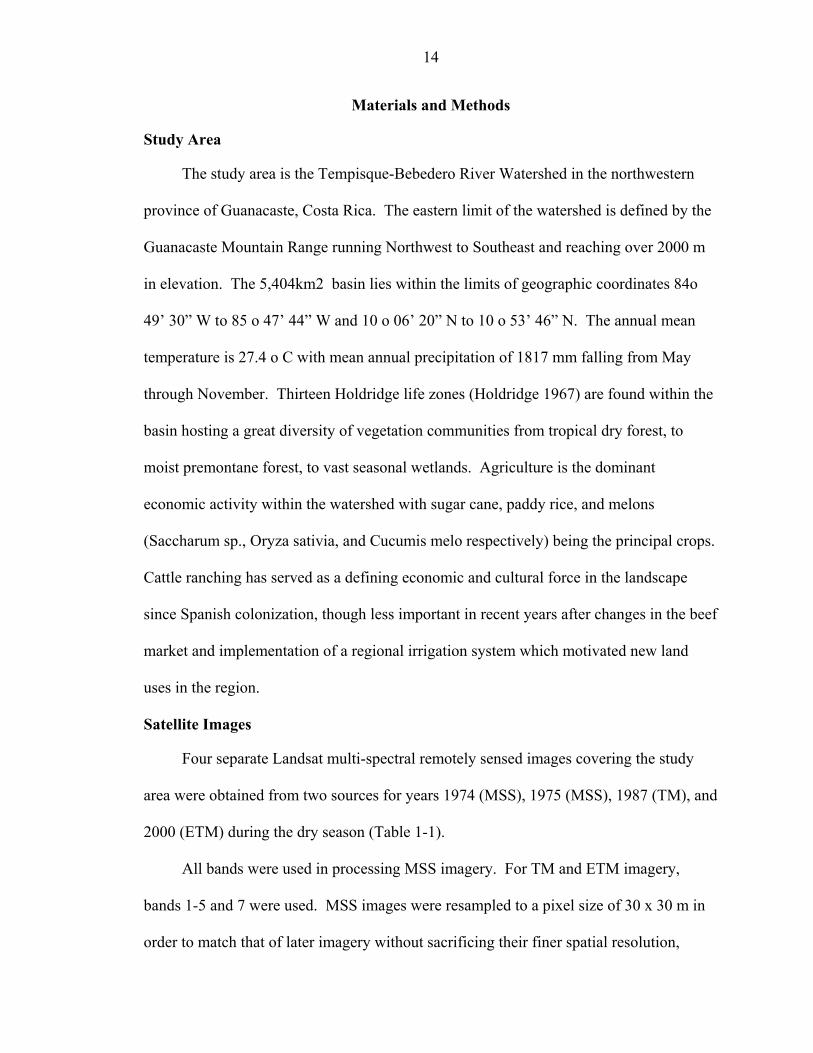
Materials and Methods

Study Area

The study area is the Tempisque-Bebedero River Watershed in the northwestern

province of Guanacaste, Costa Rica. The eastern limit of the watershed is defined by the

Guanacaste Mountain Range running Northwest to Southeast and reaching over 2000 m

in elevation. The 5,404km2 basin lies within the limits of geographic coordinates 84o

49’ 30” W to 85 o 47’ 44” W and 10 o 06’ 20” N to 10 o 53’ 46” N. The annual mean

temperature is 27.4 o C with mean annual precipitation of 1817 mm falling from May

through November. Thirteen Holdridge life zones (Holdridge 1967) are found within the

basin hosting a great diversity of vegetation communities from tropical dry forest, to

moist premontane forest, to vast seasonal wetlands. Agriculture is the dominant

economic activity within the watershed with sugar cane, paddy rice, and melons

(Saccharum sp., Oryza sativia, and Cucumis melo respectively) being the principal crops.

Cattle ranching has served as a defining economic and cultural force in the landscape

since Spanish colonization, though less important in recent years after changes in the beef

market and implementation of a regional irrigation system which motivated new land

uses in the region.

Satellite Images

Four separate Landsat multi-spectral remotely sensed images covering the study

area were obtained from two sources for years 1974 (MSS), 1975 (MSS), 1987 (TM), and

2000 (ETM) during the dry season (Table 1-1).

All bands were used in processing MSS imagery. For TM and ETM imagery,

bands 1-5 and 7 were used. MSS images were resampled to a pixel size of 30 x 30 m in

order to match that of later imagery without sacrificing their finer spatial resolution,

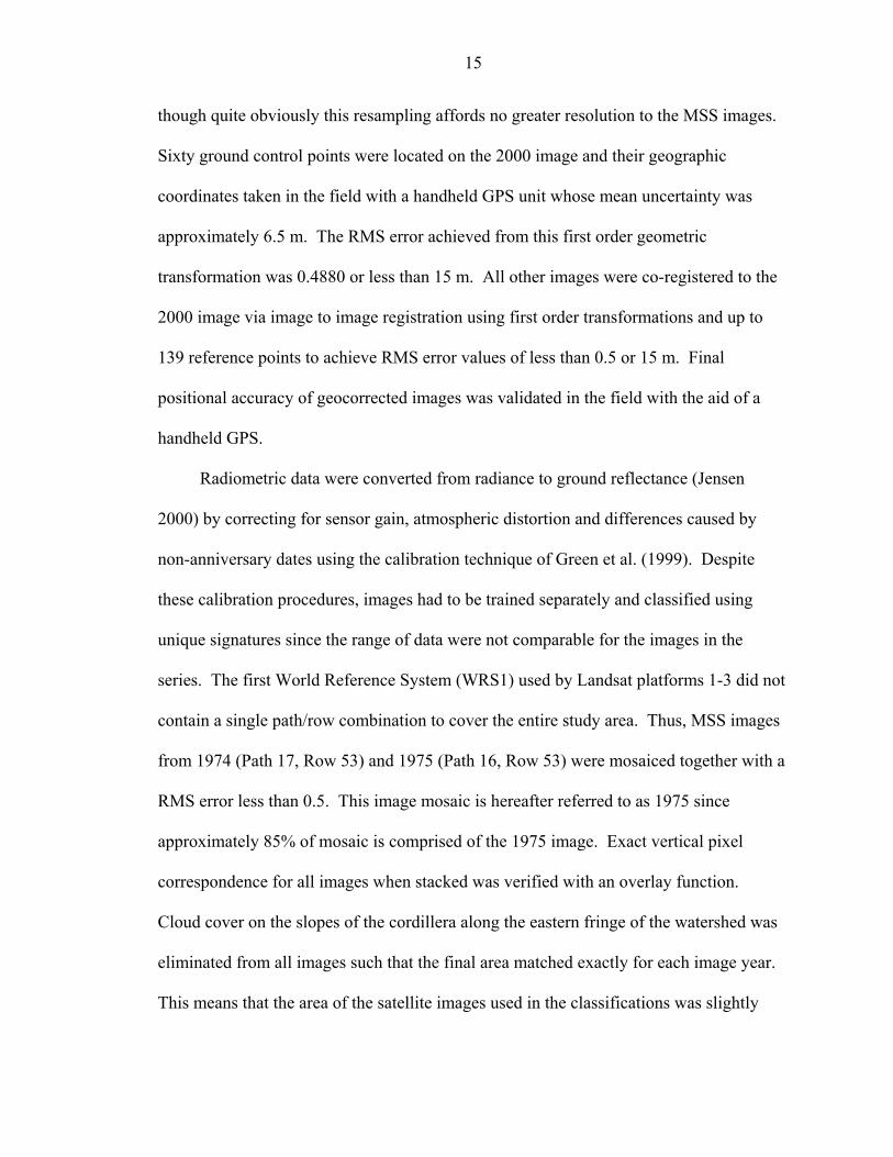
15

though quite obviously this resampling affords no greater resolution to the MSS images.

Sixty ground control points were located on the 2000 image and their geographic

coordinates taken in the field with a handheld GPS unit whose mean uncertainty was

approximately 6.5 m. The RMS error achieved from this first order geometric

transformation was 0.4880 or less than 15 m. All other images were co-registered to the

2000 image via image to image registration using first order transformations and up to

139 reference points to achieve RMS error values of less than 0.5 or 15 m. Final

positional accuracy of geocorrected images was validated in the field with the aid of a

handheld GPS.

Radiometric data were converted from radiance to ground reflectance (Jensen

2000) by correcting for sensor gain, atmospheric distortion and differences caused by

non-anniversary dates using the calibration technique of Green et al. (1999). Despite

these calibration procedures, images had to be trained separately and classified using

unique signatures since the range of data were not comparable for the images in the

series. The first World Reference System (WRS1) used by Landsat platforms 1-3 did not

contain a single path/row combination to cover the entire study area. Thus, MSS images

from 1974 (Path 17, Row 53) and 1975 (Path 16, Row 53) were mosaiced together with a

RMS error less than 0.5. This image mosaic is hereafter referred to as 1975 since

approximately 85% of mosaic is comprised of the 1975 image. Exact vertical pixel

correspondence for all images when stacked was verified with an overlay function.

Cloud cover on the slopes of the cordillera along the eastern fringe of the watershed was

eliminated from all images such that the final area matched exactly for each image year.

This means that the area of the satellite images used in the classifications was slightly

16

less than the true extent of the watershed. All image processing was carried out using

ERDAS Imagine 8.5.

Precipitation Data

Vegetation biomass is positively correlated with precipitation (Fang et al. 2001).

Precipitation trends prior to image capture have been shown to affect red and near-

infrared band reflectance (Ji and Peters. 2004). The Pacific slope of Costa Rica

experiences both drought and periods of unusually high rainfall and flooding associated

with ENSO events (Waylen and Laporte 1999). In order to take into account the effects

of climatic variability on land cover dynamics throughout the temporal and spatial extents

of the study, precipitation data were compiled from seven meteorological stations

managed by the Costa Rican Institute of Electricity (Instituto Costaricense de

Electricidad, ICE) and the National Meteorological Institute (Instituto Meteorológico

Nacional, IMN).

A time series of precipitation across the entire study period was constructed using

the mean of several meteorological stations positioned throughout the watershed

[Appendix A]. The 12 months and roughly 30 days preceding the date of each image

were highlighted to examine how image years fit in with overall climate patterns. Also,

mean monthly precipitation was calculated, using a greater number of stations, for the

twelve months preceding each image date and also that for the thirty preceding days

[Appendix A]. Precipitation for the 12 months preceding the 1987 image was

substantially lower than that of the other image dates (99.36 mm/month versus 132.92

mm/month and 192.49 mm/month for 1975 and 2000 respective), but since the image

was taken at the beginning of the dry season, the preceding 30-day average was

substantially higher (27.8 mm versus 0 mm and 2.19 mm for 1975 and 2000,

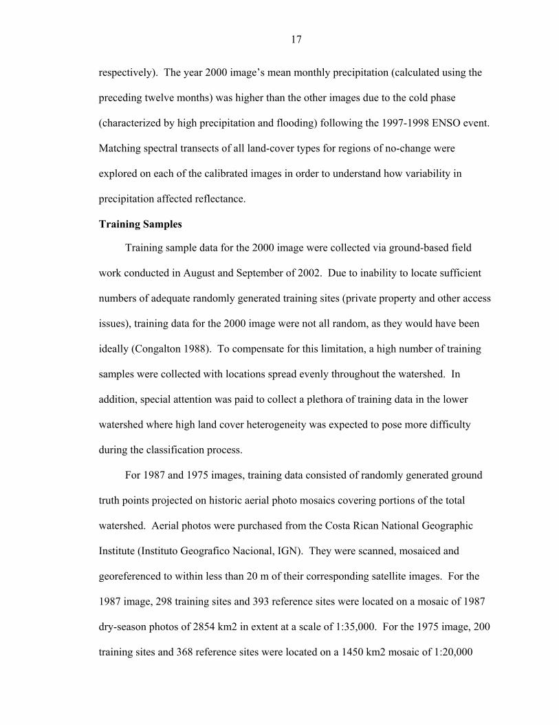
17

respectively). The year 2000 image’s mean monthly precipitation (calculated using the

preceding twelve months) was higher than the other images due to the cold phase

(characterized by high precipitation and flooding) following the 1997-1998 ENSO event.

Matching spectral transects of all land-cover types for regions of no-change were

explored on each of the calibrated images in order to understand how variability in

precipitation affected reflectance.

Training Samples

Training sample data for the 2000 image were collected via ground-based field

work conducted in August and September of 2002. Due to inability to locate sufficient

numbers of adequate randomly generated training sites (private property and other access

issues), training data for the 2000 image were not all random, as they would have been

ideally (Congalton 1988). To compensate for this limitation, a high number of training

samples were collected with locations spread evenly throughout the watershed. In

addition, special attention was paid to collect a plethora of training data in the lower

watershed where high land cover heterogeneity was expected to pose more difficulty

during the classification process.

For 1987 and 1975 images, training data consisted of randomly generated ground

truth points projected on historic aerial photo mosaics covering portions of the total

watershed. Aerial photos were purchased from the Costa Rican National Geographic

Institute (Instituto Geografico Nacional, IGN). They were scanned, mosaiced and

georeferenced to within less than 20 m of their corresponding satellite images. For the

1987 image, 298 training sites and 393 reference sites were located on a mosaic of 1987

dry-season photos of 2854 km2 in extent at a scale of 1:35,000. For the 1975 image, 200

training sites and 368 reference sites were located on a 1450 km2 mosaic of 1:20,000

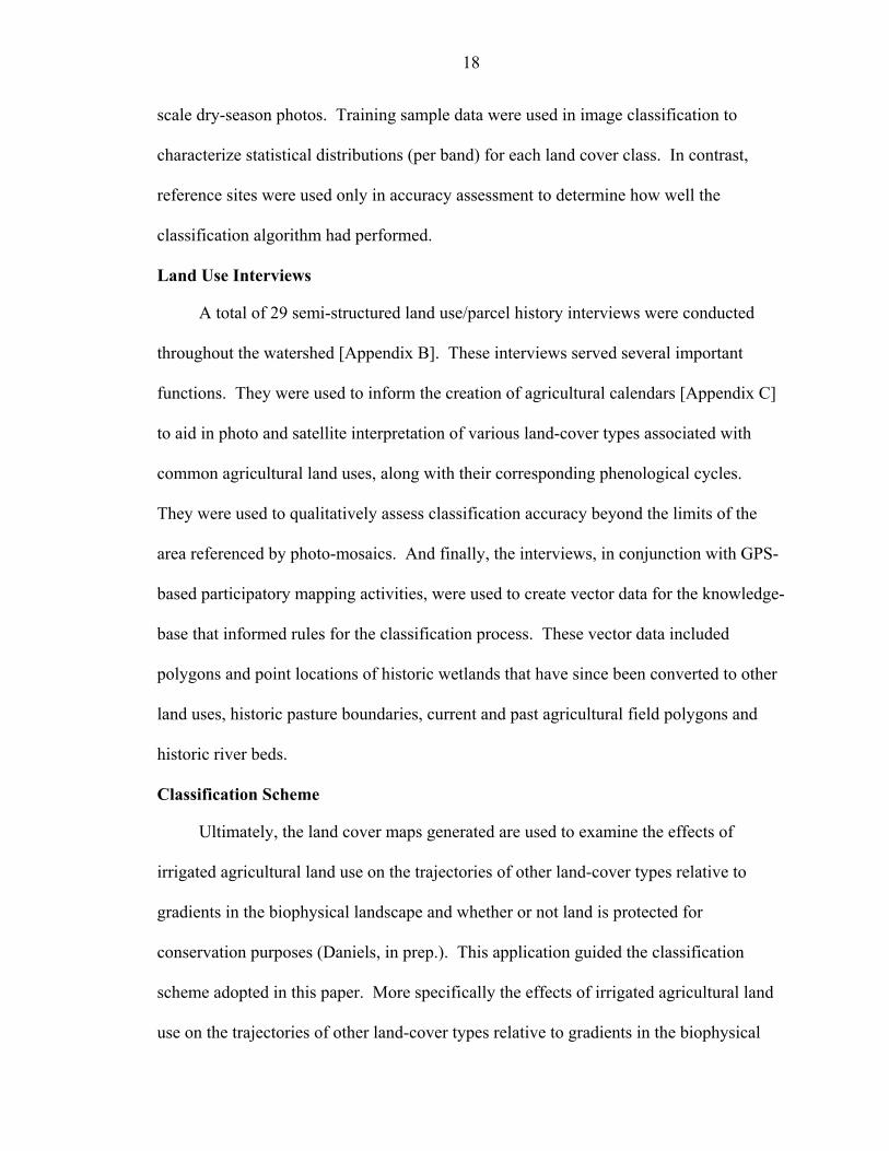
18

scale dry-season photos. Training sample data were used in image classification to

characterize statistical distributions (per band) for each land cover class. In contrast,

reference sites were used only in accuracy assessment to determine how well the

classification algorithm had performed.

Land Use Interviews

A total of 29 semi-structured land use/parcel history interviews were conducted

throughout the watershed [Appendix B]. These interviews served several important

functions. They were used to inform the creation of agricultural calendars [Appendix C]

to aid in photo and satellite interpretation of various land-cover types associated with

common agricultural land uses, along with their corresponding phenological cycles.

They were used to qualitatively assess classification accuracy beyond the limits of the

area referenced by photo-mosaics. And finally, the interviews, in conjunction with GPS-

based participatory mapping activities, were used to create vector data for the knowledge-

base that informed rules for the classification process. These vector data included

polygons and point locations of historic wetlands that have since been converted to other

land uses, historic pasture boundaries, current and past agricultural field polygons and

historic river beds.

Classification Scheme

Ultimately, the land cover maps generated are used to examine the effects of

irrigated agricultural land use on the trajectories of other land-cover types relative to

gradients in the biophysical landscape and whether or not land is protected for

conservation purposes (Daniels, in prep.). This application guided the classification

scheme adopted in this paper. More specifically the effects of irrigated agricultural land

use on the trajectories of other land-cover types relative to gradients in the biophysical

19

landscape are examined. As such, the final information classes of interest were

comprised of an amalgam of both land cover and land use classes. Land cover classes

employed were water (representing open, non-vegetated wetlands), vegetated wetlands,

grasslands, and forest. Land use classes were urban and irrigated agriculture. For land

use classes, several distinct land cover classes were grouped under their headings, aided

by the agricultural calendars created with land use interviews. Specifically, the

information classes of interest were defined as follows:

• Irrigated agriculture: Dominant land covers include irrigated crops Oryza sativia (rice), Saccharum sp. (sugar cane), Cucumis melo (mellon), bare soil, water (flooded rice fields prior to germination), and cachaza (by-product of sugar refinement used as an organic fertilizer). Minor crops include Cucumis sativus (cucumber) and Allium cepa (onion). Agricultural calendars [Appendix C] offer chronology and detailed descriptions of land cover throughout each major crop’s planting cycle.

• Water: This class was intended to correspond to the land cover of non- or sparsely vegetated wetlands. However, several phenological phases of flooded rice cultivation gave nearly or precisely the same reflectance signals. Thus, pixels described by the latter case were properly classified into desired information classes through the rule-based algorithm, despite that the actual land cover and spectral classes were nearly identical.

• Vegetated Wetlands: The Ramsar interpretation of wetlands was adopted for the purpose of defining wetland land cover in this study.1 A great diversity of flood regimes and hydroperiods is evidenced by myriad types of wetland communities. The Tempisque Watershed has lotic systems, mangroves, flooded forests, fresh marshes and fresh meadows. Vegetation community characterizations of the various wetland communities is found in Appendix D.

• Urban: This land use class covers all anthropogenic land cover in population centers. For example, spectral classes for urban land use include those of mixed concrete and asphalt and residential areas (mixed vegetation and houses). Because of the heterogeneity of reflectance surfaces within each pixel area, nearly all of the spectral classes for urban land use were comprised of averaged spectral signals for a given 30 x 30 m area.

1 “Wetlands are areas of marsh, fen, peatland or water, whether natural or artificial, permanent or temporary, with water that is static or flowing, fresh, brackish or salt, including areas of marine water the depth of which at low tide does not exceed six meters” (Article 1.1, Ramsar Convention on Wetlands, 1971).

20

• Grasslands: This land cover class was divided into sub-groups, the first three in which land use largely determined dominant vegetation and thus reflectance characteristics. These sub-groups were as follows: strict pasture (often actively managed) with grasses only, pasture with occasional trees, recently fallowed pasture (approximately < 3years) that was still largely dominated by grasses, grassy areas where soils or fire frequency does not support abundant tree growth (e.g., areas of volcanic slopes) and finally, miscellaneous grasses lining roads and other public works. Vegetation characterization of each type is found in Appendix D.

• Forest: The diversity of Holdridge Life Zones and biophysical niches in the watershed is evidenced by myriad forest types. The watershed is characterized by limestone forest, deciduous lowland forest, evergreen lowland forest and pre-montane moist forest. Rainy season canopy closure of > 40% was required to qualify as forest land cover. Vegetation community characterizations of each type of forest is found in Appendix D

Land-cover classifications

Spectral signatures were created for the six information land cover and land use

classes of interest (irrigated agriculture, water, vegetated wetlands, urban, grassland,

forest) using the training data gathered from field work (for 2000) or from photo-

interpreted training data (for 1987 and 1975). Each information class was comprised of a

number of spectral classes since a single information class may represent more than one

successional or phenological stage of its land-cover type, etc. Classifications were

performed using two distinct algorithms: the Gaussian maximum-likelihood classifier

and the parallelepiped classifier. The former is a relative classification algorithm that

relies on effective training data from all classes and assumes that reflectance data for each

class in each band has a Gaussian distribution (Jensen 2000). This algorithm is more

robust since it takes the covariance of the data into consideration (Ozesmi and Bauer

2002). However, not all data are normally distributed and this classifier can perform

quite poorly in such cases.

The parallelepiped classifier is an absolute algorithm wherein each pixel meeting

the defined upper and lower limits for each band for a given class, is assigned to that

21

class. The major drawback with this algorithm is that the n-dimensional spaces defined

by such upper and lower limits for n bands often overlap for different classes (Jensen

1996). A given pixel is then assigned to the first class for which it meets the criteria (i.e.,

assignment by order). However, due to the non-normal distributions in one or more

spectral classes comprising wetland, grassland and forest information classes, a separate

classification using the parallelepiped algorithm was produced. The purpose of the

parallelpiped classification was for incorporation into the rule-based classification for

non-normally distributed data.

Other Data and Knowledge Base

Other data included a digital elevation model (DEM) of 30m spatial resolution (x,y)

and 1m elevation resolution (z) which was obtained from the OTS Palo Verde Research

Station. From this, a slope model was produced. Normalized Differenced Vegetation

Index (NDVI) layers were produced that indirectly give an indication of the amount of

biomass on a per-pixel basis. For TM imagery NDVI is calculated as (band 4 – band3)/

(band 4 + band 3) and as (band 4 – band 2)/ (band 4 + band 2) for MSS imagery.

A layer of point coordinates for all population centers was created using a GPS to

record the location of each town center. Identification of population centers was

informed by topographic maps of 1:50,000 scale (updated various years from 1974 to

1987). Polygons of agricultural fields of large landholders were created through photo-

interpretation of the aerial photo-mosaics for 1975 and 1987. All current and, where

possible, past agricultural fields/major landholdings were mapped in the field using a

GPS and the assistance of employees on large-scale agricultural operations, along with

manual interpretation of the 2000 satellite image.

22

Three spatial analyses were performed whose products were used in the rule-based

algorithms to afford the classification process logical reasoning with regard to domain

knowledge. The first model created a raster surface dividing all pixels into one of two

groups: those that fall within the bounds of agricultural fields (as defined by created

polygons) and all others. Similarly, the second model produced a raster surface which

divided all pixels into those that fell within the defined buffer around population center

coordinates (of varying radii depending on the size of the town) and all others. The third

spatial model isolated all water pixels in the Tempisque and Bebedero Rivers and

calculated the nearest distance to river pixels from every other pixel in the watershed.

When coupled with other criteria, the surfaces created with these models provide a means

of incorporating spatial context and association into automated algorithms. These and all

other ancillary data comprising the knowledge base upon which the class domains, and

thus classification rules were based, are summarized in Table 2-1.

Processing Flow for Rule-Based Classifications

As mentioned above, the maximum likelihood and parallelepiped classifiers each

have advantages and disadvantages. The methodology proposed in this paper,

summarized in Figure 2-1, is novel in that it employs a simple, rule-based, classification

technique wherein the advantages of the parallelepiped and maximum likelihood

classifiers, along with domain knowledge, are combined without resorting to advanced

statistical approaches developed for unique scenarios like partial classifications (see

Fernandez-Prieto 2002). Furthermore, logic-oriented processing is afforded by the

incorporation of domain knowledge and landscape contextual information via IF/THEN

Boolean logic rules. Such advantages and disadvantages of the proposed technique

relative to using a single classifier alone are summarized in Table2-2.

23

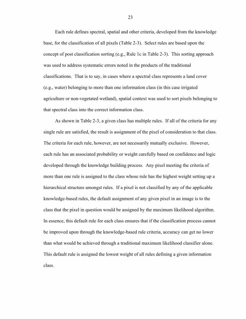
Each rule defines spectral, spatial and other criteria, developed from the knowledge

base, for the classification of all pixels (Table 2-3). Select rules are based upon the

concept of post classification sorting (e.g., Rule 1c in Table 2-3). This sorting approach

was used to address systematic errors noted in the products of the traditional

classifications. That is to say, in cases where a spectral class represents a land cover

(e.g., water) belonging to more than one information class (in this case irrigated

agriculture or non-vegetated wetland), spatial context was used to sort pixels belonging to

that spectral class into the correct information class.

As shown in Table 2-3, a given class has multiple rules. If all of the criteria for any

single rule are satisfied, the result is assignment of the pixel of consideration to that class.

The criteria for each rule, however, are not necessarily mutually exclusive. However,

each rule has an associated probability or weight carefully based on confidence and logic

developed through the knowledge building process. Any pixel meeting the criteria of

more than one rule is assigned to the class whose rule has the highest weight setting up a

hierarchical structure amongst rules. If a pixel is not classified by any of the applicable

knowledge-based rules, the default assignment of any given pixel in an image is to the

class that the pixel in question would be assigned by the maximum likelihood algorithm.

In essence, this default rule for each class ensures that if the classification process cannot

be improved upon through the knowledge-based rule criteria, accuracy can get no lower

than what would be achieved through a traditional maximum likelihood classifier alone.

This default rule is assigned the lowest weight of all rules defining a given information

class.

24

Accuracy Assessment

Standard accuracy assessment was performed for all images wherein independent

reference test pixels based on fieldwork (for 2000 image) or photointerpretation (for 1975

and 1987) were compared with the classification results. Reference pixels were obtained

in two rounds: one round concomitant with training samples and one round of additional

points after stratifying the landscape according to land cover categories. Accuracy was

assessed for the products of traditional classifiers and for the proposed method in order to

determine the level of improvement afforded by the rule-based technique. Indeed, some

of the post-classification sorting rules (such as Rule 3c) were informed through careful

assessment of errors observed in the matrices and classified image from the maximum

likelihood classification. All accuracy assessment was based on comparisons at the

information class level since that was the maximum taxonomic resolution gathered for

reference points. That is to say, spectral classes were merged into their corresponding

information classes for accuracy assessment.

Measures of classification performance calculated in the accuracy assessment

process included overall accuracy, class-wise producer’s accuracy (index of errors of

omission), class-wise user’s accuracy (index of errors of commission) and both overall

and class-wise KAPPA statistics (see formula in Appendix E).

Results

Comparing results from the traditional maximum likelihood classifier versus the

rule-based product (Figure 2) shows unambiguous improvement in both producer’s and

user’s accuracies, along with substantial improvement in the Kappa coefficient (Table 2-

4). This trend holds for each class-wise comparison for each year (Figure 3) as well as

the overall classification comparisons per year (Table 2-4). Overall accuracy and Kappa

25

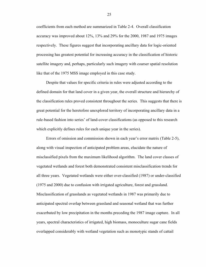
coefficients from each method are summarized in Table 2-4. Overall classification

accuracy was improved about 12%, 13% and 29% for the 2000, 1987 and 1975 images

respectively. These figures suggest that incorporating ancillary data for logic-oriented

processing has greatest potential for increasing accuracy in the classification of historic

satellite imagery and, perhaps, particularly such imagery with coarser spatial resolution

like that of the 1975 MSS image employed in this case study.

Despite that values for specific criteria in rules were adjusted according to the

defined domain for that land cover in a given year, the overall structure and hierarchy of

the classification rules proved consistent throughout the series. This suggests that there is

great potential for the heretofore unexplored territory of incorporating ancillary data in a

rule-based fashion into series’ of land-cover classifications (as opposed to this research

which explicitly defines rules for each unique year in the series).

Errors of omission and commission shown in each year’s error matrix (Table 2-5),

along with visual inspection of anticipated problem areas, elucidate the nature of

misclassified pixels from the maximum likelihood algorithm. The land cover classes of

vegetated wetlands and forest both demonstrated consistent misclassification trends for

all three years. Vegetated wetlands were either over-classified (1987) or under-classified

(1975 and 2000) due to confusion with irrigated agriculture, forest and grassland.

Misclassification of grasslands as vegetated wetlands in 1987 was primarily due to

anticipated spectral overlap between grassland and seasonal wetland that was further

exacerbated by low precipitation in the months preceding the 1987 image capture. In all

years, spectral characteristics of irrigated, high biomass, monoculture sugar cane fields

overlapped considerably with wetland vegetation such as monotypic stands of cattail

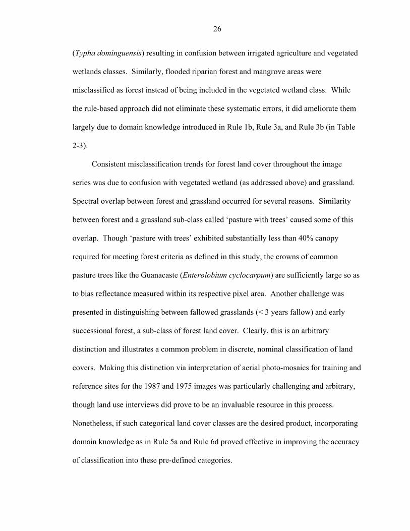
26

(Typha dominguensis) resulting in confusion between irrigated agriculture and vegetated

wetlands classes. Similarly, flooded riparian forest and mangrove areas were

misclassified as forest instead of being included in the vegetated wetland class. While

the rule-based approach did not eliminate these systematic errors, it did ameliorate them

largely due to domain knowledge introduced in Rule 1b, Rule 3a, and Rule 3b (in Table

2-3).

Consistent misclassification trends for forest land cover throughout the image

series was due to confusion with vegetated wetland (as addressed above) and grassland.

Spectral overlap between forest and grassland occurred for several reasons. Similarity

between forest and a grassland sub-class called ‘pasture with trees’ caused some of this

overlap. Though ‘pasture with trees’ exhibited substantially less than 40% canopy

required for meeting forest criteria as defined in this study, the crowns of common

pasture trees like the Guanacaste (Enterolobium cyclocarpum) are sufficiently large so as

to bias reflectance measured within its respective pixel area. Another challenge was

presented in distinguishing between fallowed grasslands (< 3 years fallow) and early

successional forest, a sub-class of forest land cover. Clearly, this is an arbitrary

distinction and illustrates a common problem in discrete, nominal classification of land

covers. Making this distinction via interpretation of aerial photo-mosaics for training and

reference sites for the 1987 and 1975 images was particularly challenging and arbitrary,

though land use interviews did prove to be an invaluable resource in this process.

Nonetheless, if such categorical land cover classes are the desired product, incorporating

domain knowledge as in Rule 5a and Rule 6d proved effective in improving the accuracy

of classification into these pre-defined categories.

27

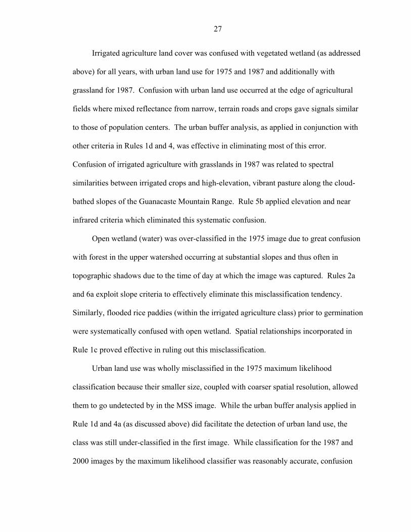
Irrigated agriculture land cover was confused with vegetated wetland (as addressed

above) for all years, with urban land use for 1975 and 1987 and additionally with

grassland for 1987. Confusion with urban land use occurred at the edge of agricultural

fields where mixed reflectance from narrow, terrain roads and crops gave signals similar

to those of population centers. The urban buffer analysis, as applied in conjunction with

other criteria in Rules 1d and 4, was effective in eliminating most of this error.

Confusion of irrigated agriculture with grasslands in 1987 was related to spectral

similarities between irrigated crops and high-elevation, vibrant pasture along the cloud-

bathed slopes of the Guanacaste Mountain Range. Rule 5b applied elevation and near

infrared criteria which eliminated this systematic confusion.

Open wetland (water) was over-classified in the 1975 image due to great confusion

with forest in the upper watershed occurring at substantial slopes and thus often in

topographic shadows due to the time of day at which the image was captured. Rules 2a

and 6a exploit slope criteria to effectively eliminate this misclassification tendency.

Similarly, flooded rice paddies (within the irrigated agriculture class) prior to germination

were systematically confused with open wetland. Spatial relationships incorporated in

Rule 1c proved effective in ruling out this misclassification.

Urban land use was wholly misclassified in the 1975 maximum likelihood

classification because their smaller size, coupled with coarser spatial resolution, allowed

them to go undetected by in the MSS image. While the urban buffer analysis applied in

Rule 1d and 4a (as discussed above) did facilitate the detection of urban land use, the

class was still under-classified in the first image. While classification for the 1987 and

2000 images by the maximum likelihood classifier was reasonably accurate, confusion

28

with irrigated agriculture for these years was eliminated (see above) and misclassification

of grasslands as urban was ruled out via application of the urban buffer model in Rule 5c.

Finally, grassland land cover was confused with several classes as has been

discussed in the context of these classes’ misclassification tendencies above. Though

domain knowledge applied in the rule-based approach definitely enhanced the ability to

discern between confused classes, classifications from the rule-based method still

demonstrated slight misclassification with forest (1975 and 1987) and vegetated wetland

(2000).

Discussion

Consistent with many other studies employing ancillary data in the classification

process, the proposed rule-based approach suggests that incorporation of appropriate

domain knowledge is an effective way of achieving high classification accuracy for

complex, heterogeneous landscapes such as the Tempisque Watershed. One of the

shortcomings of the proposed methodology is that, despite final digital/automated

algorithms, the logic behind each rule was derived through an extensive process relying

on human interpretation of complex datasets. The costs and benefits of classification

improvement via logic-based processing and incorporation of domain knowledge must be

carefully considered.

Murai and Omatu (1997) employed a neural network, pattern-recognition algorithm

on spectral data alone and then incorporated a rule-based correction phase reliant upon

geographical knowledge that reduced misclassifications due to cloud shadows and

averaged reflectance over a given pixel’s ground area. While this method was

computationally more complex than that proposed in the current paper, intelligent

processing was achieved in a semi-automated fashion (the advantage of any form of true

29

artificial intelligence). In contrast to the landscape contextual approach emphasized here,

geographical knowledge was limited to using adjacent pixel associations in the form of

pixel neighborhoods, a top-down approach that incorporates no new or independent

information to complement satellite data. However, the actual utility of integrating pixel

associations was afforded by human reasoning. That is to say the construction of

IF/THEN rules was still largely dependent upon human input. The error correction rule-

based algorithms eliminated some but not all error.

Other studies have reported no improvement in accuracy as a result of

incorporating additional data for consideration in the classification criteria or algorithm

employed. Southworth (2004) explored the utility of incorporating thermal data in

classification of land cover in the dry forest region of Yucatan, Mexico. While

blackbody temperatures were show to be strongly correlated with land cover classes and

have great potential in land cover analysis, the incorporation of thermal data did not

statistically improve classification results over what was achieved with spectral data

alone. Similarly, Sader et al. (1995) developed a hierarchical, rule-based method for the

classification of forested wetlands. The classification rules integrated spectral data,

National Wetlands Inventory (NWI) maps, a DEM, a slope model, hydrography, hydric

soil data, and association/location. Despite this exhaustive ancillary dataset,

classification results from the rule-based classifier did not have improved accuracy over a

conventional hybrid classification.

Clearly, the utility and outcome of any cost/benefit analysis when considering the

use of ancillary data and logic-oriented classification techniques depends upon landscape

structure, desired accuracy, and geographic context, amongst myriad other factors.

30

Insufficient exploration has been performed of when, where, how and which ancillary

data is useful to attempt to construct any valid heuristics. Moreover, many studies

employing alternative classification techniques, including logic-oriented or intelligent

processing do not focus explicitly on exploring the utility of the employed methodology

for accuracy improvement. Thus they do not compare achieved results with traditional

products (e.g., De Fries et al. 1998, Vogelmann et al. 1998, Murai and Omatu 1997).

This makes it difficult to use the literature as a resource when exploring the possible

techniques for classification during the exploratory/training phase of remote sensing

studies.

Conclusion

The primary objective of this research was to explore the utility of incorporating

domain knowledge into a rule-based classification technique for accuracy improvement

by comparing results from the proposed technique with those of maximum likelihood

classifications on spectral data alone. Secondary objectives were to illustrate the

advantages of integrating domain knowledge informed by ancillary data, along with more

than one traditional classifier, in the classification of problematic tropical land cover and

to demonstrate a methodology for logic-oriented processing of historic satellite imagery.

Classification accuracy was unequivocally improved for all classes and all years of the

classification series relative to the results from the traditional maximum likelihood

method. Domain knowledge constructed from interpreting and integrating ancillary data

facilitated the correct classification of challenging tropical land cover like dry tropical

forest and seasonal wetlands. Finally, results from this research suggest that not only are

ancillary data valuable in the classification of historic satellite imagery, but perhaps this

is where their greatest utility lies.

31

The major cost of the proposed rule-based technique is in the time involved in

creating spatial data layers and the degree of knowledge necessary about land-

management systems and land tenure across the spatial and temporal extent of the study

period. However, as GIS becomes increasingly employed by local institutions in tropical

regions, much of the data and knowledge may be available for future applications of such

knowledge-based applications. The final accuracies of rule-based classifications across

all dates in the study are amongst the highest in literature on land-cover classifications for

the tropics. Moreover, this method allows for the accurate classification of all major land

covers rather than the more commonly used forest/non-forest dichotomy. Anticipated

extensions of this research include more rigorous statistical analyses of the optimal

number of rules used for each information class to better determine the threshold at which

increasing knowledge of land cover domains and processing efforts deliver little

improvement in accuracy.

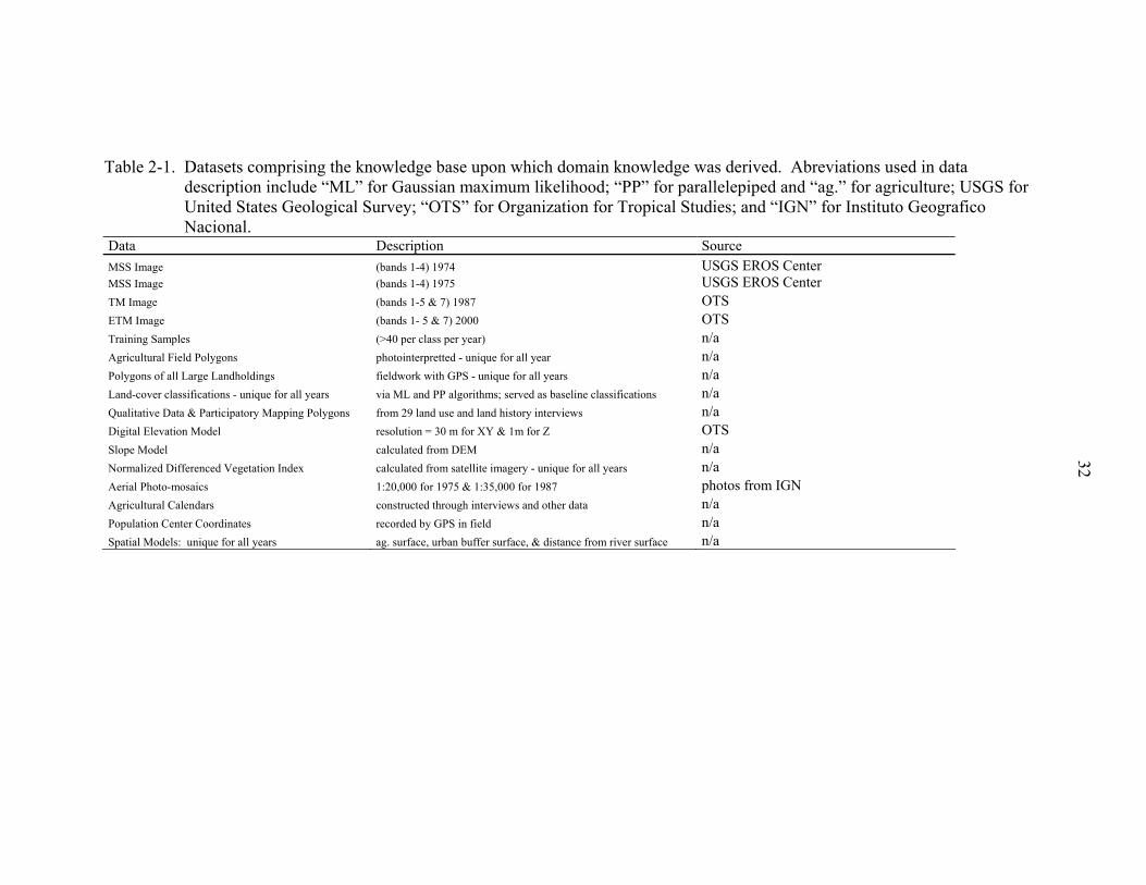
32

Table 2-1. Datasets comprising the knowledge base upon which domain knowledge was derived. Abreviations used in data description include “ML” for Gaussian maximum likelihood; “PP” for parallelepiped and “ag.” for agriculture; USGS for United States Geological Survey; “OTS” for Organization for Tropical Studies; and “IGN” for Instituto Geografico Nacional.

Data Description SourceMSS Image (bands 1-4) 1974 USGS EROS Center MSS Image (bands 1-4) 1975 USGS EROS Center TM Image (bands 1-5 & 7) 1987 OTS ETM Image (bands 1- 5 & 7) 2000 OTS Training Samples (>40 per class per year) n/a Agricultural Field Polygons photointerpretted - unique for all year n/a Polygons of all Large Landholdings fieldwork with GPS - unique for all years n/a Land-cover classifications - unique for all years via ML and PP algorithms; served as baseline classifications n/a Qualitative Data & Participatory Mapping Polygons from 29 land use and land history interviews n/a Digital Elevation Model resolution = 30 m for XY & 1m for Z OTS Slope Model calculated from DEM n/a Normalized Differenced Vegetation Index calculated from satellite imagery - unique for all years n/a Aerial Photo-mosaics 1:20,000 for 1975 & 1:35,000 for 1987 photos from IGN Agricultural Calendars constructed through interviews and other data n/a Population Center Coordinates recorded by GPS in field n/a Spatial Models: unique for all years ag. surface, urban buffer surface, & distance from river surface n/a

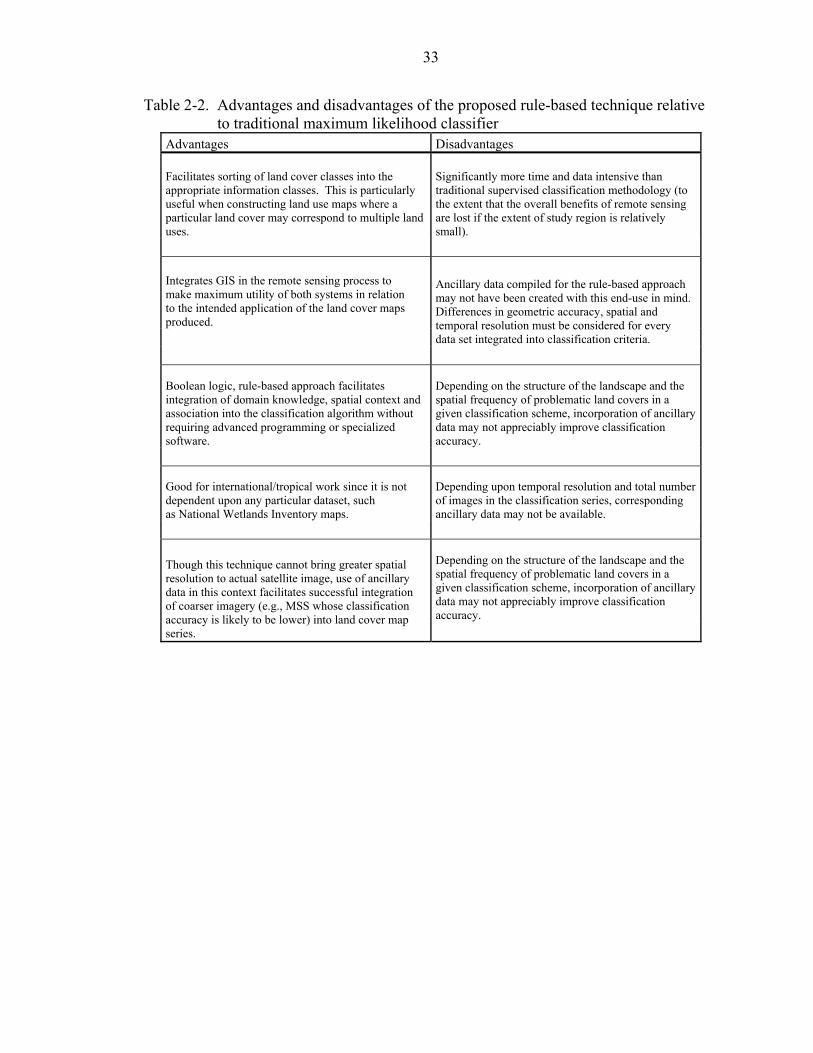
33

Table 2-2. Advantages and disadvantages of the proposed rule-based technique relative to traditional maximum likelihood classifier

Advantages Disadvantages

Facilitates sorting of land cover classes into the appropriate information classes. This is particularly useful when constructing land use maps where a particular land cover may correspond to multiple land uses.

Significantly more time and data intensive than traditional supervised classification methodology (to the extent that the overall benefits of remote sensing are lost if the extent of study region is relatively small).

Integrates GIS in the remote sensing process to make maximum utility of both systems in relation to the intended application of the land cover maps produced.

Ancillary data compiled for the rule-based approach may not have been created with this end-use in mind. Differences in geometric accuracy, spatial and temporal resolution must be considered for every data set integrated into classification criteria.

Boolean logic, rule-based approach facilitates integration of domain knowledge, spatial context and association into the classification algorithm without requiring advanced programming or specialized software.

Depending on the structure of the landscape and the spatial frequency of problematic land covers in a given classification scheme, incorporation of ancillary data may not appreciably improve classification accuracy.

Good for international/tropical work since it is not dependent upon any particular dataset, such as National Wetlands Inventory maps.

Depending upon temporal resolution and total numberof images in the classification series, corresponding ancillary data may not be available.

Depending on the structure of the landscape and the spatial frequency of problematic land covers in a given classification scheme, incorporation of ancillary data may not appreciably improve classification accuracy.

Though this technique cannot bring greater spatial resolution to actual satellite image, use of ancillary data in this context facilitates successful integration of coarser imagery (e.g., MSS whose classification accuracy is likely to be lower) into land cover map series.

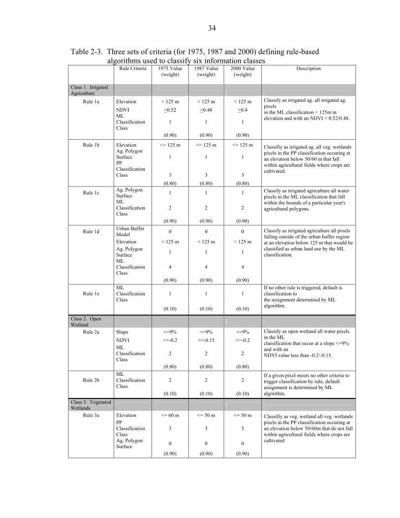
34

Table 2-3. Three sets of criteria (for 1975, 1987 and 2000) defining rule-based algorithms used to classify six information classes

Rule Criteria

1975 Value (weight)

1987 Value (weight)

2000 Value (weight)

Description

Class 1. Irrigated Agriculture

Rule 1a Elevation < 125 m < 125 m < 125 m NDVI >0.52 >0.48 >0.4

ML Classification Class

1 1 1

(0.90) (0.90) (0.90)

Classify as irrigated ag. all irrigated ag. pixels in the ML classification < 125m in elevation and with an NDVI < 0.52/0.48.

Rule 1b Elevation <= 125 m <= 125 m <= 125 m

Ag. Polygon Surface 1 1 1

PP Classification Class 3 3 3

(0.80) (0.80) (0.80)

Classifiy as irrigated ag. all veg. wetlands pixels in the PP classification occuring at an elevation below 50/60 m that fall within agricultural fields where crops are cultivated.

Rule 1c Ag. Polygon Surface 1 1 1

ML Classification Class

2 2 2

(0.90) (0.90) (0.90)

Classify as irrigated agriculture all water pixels in the ML classification that fall within the bounds of a particular year's agricultural polygons.

Rule 1d Urban Buffer Model 0 0 0

Elevation < 125 m < 125 m < 125 m

Ag. Polygon Surface 1 1 1

ML Classification Class

4 4 4

(0.90) (0.90) (0.90)

Classify as irrigated agriculture all pixels falling outside of the urban buffer region at an elevation below 125 m that would be classified as urban land use by the ML classification.

Rule 1e ML Classification Class

1 1 1

(0.10) (0.10) (0.10)

If no other rule is triggered, default is classification to the assignment determined by ML algorithm.

Class 2. Open Wetland

Rule 2a Slope <=9% <=9% <=9% NDVI <=-0.2 <=-0.15 <=-0.2

ML Classification Class

2 2 2

(0.80) (0.80) (0.80)

Classify as open wetland all water pixels in the ML classification that occur at a slope <=9% and with an NDVI value less than -0.2/-0.15.

Rule 2b ML Classification Class

2 2 2

(0.10) (0.10) (0.10)

If a given pixel meets no other criteria to trigger classification by rule, default assignment is determined by ML algorithm.

Class 3. Vegetated Wetlands

Rule 3a Elevation <= 60 m <= 50 m <= 50 m

PP Classification Class

3 3 3

Ag. Polygon Surface 0 0 0

(0.90) (0.90) (0.90)

Classifiy as veg. wetland all veg. wetlands pixels in the PP classification occuring at an elevation below 50/60m that do not fall within agricultural fields where crops are cultivated

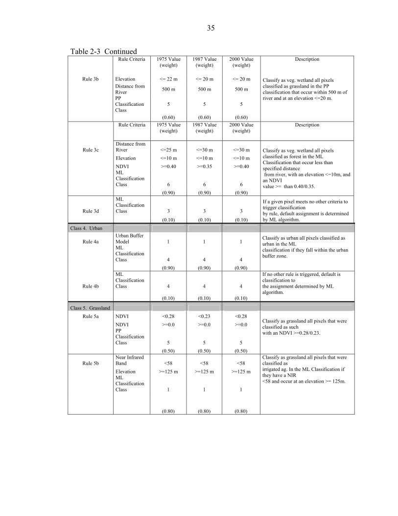
35

Table 2-3 Continued

Rule Criteria

1975 Value (weight)

1987 Value (weight)

2000 Value (weight)

Description

Rule 3b Elevation <= 22 m <= 20 m <= 20 m

Distance from River 500 m 500 m 500 m

PP Classification Class

5 5 5

(0.60) (0.60) (0.60)

Classify as veg. wetland all pixels classified as grassland in the PP classification that occur within 500 m of river and at an elevation <=20 m.

Rule Criteria

1975 Value (weight)

1987 Value (weight)

2000 Value (weight)

Description

Rule 3c Distance from River <=25 m <=30 m <=30 m

Elevation <=10 m <=10 m <=10 m NDVI >=0.40 >=0.35 >=0.40

ML Classification Class 6 6 6

(0.90) (0.90) (0.90)

Classify as veg. wetland all pixels classified as forest in the ML Classification that occur less than specified distance from river, with an elevation <=10m, and an NDVI value >= than 0.40/0.35.

Rule 3d

ML Classification Class 3 3 3

(0.10) (0.10) (0.10)

If a given pixel meets no other criteria to trigger classification by rule, default assignment is determined by ML algorithm.

Class 4. Urban

Rule 4a Urban Buffer Model 1 1 1

ML Classification Class 4 4 4

(0.90) (0.90) (0.90)

Classify as urban all pixels classified as urban in the ML classification if they fall within the urban buffer zone.

Rule 4b

ML Classification Class 4 4 4

(0.10) (0.10) (0.10)

If no other rule is triggered, default is classification to the assignment determined by ML algorithm.

Class 5. Grassland Rule 5a NDVI <0.28 <0.23 <0.28

NDVI >=0.0 >=0.0 >=0.0

PP Classification Class 5 5 5

(0.50) (0.50) (0.50)

Classify as grassland all pixels that were classified as such with an NDVI >=0.28/0.23.

Rule 5b Near Infrared Band <58 <58 <58

Elevation >=125 m >=125 m >=125 m

ML Classification Class 1 1 1

(0.80) (0.80) (0.80)

Classify as grassland all pixels that were classified as irrigated ag. In the ML Classification if they have a NIR <58 and occur at an elevation >= 125m.

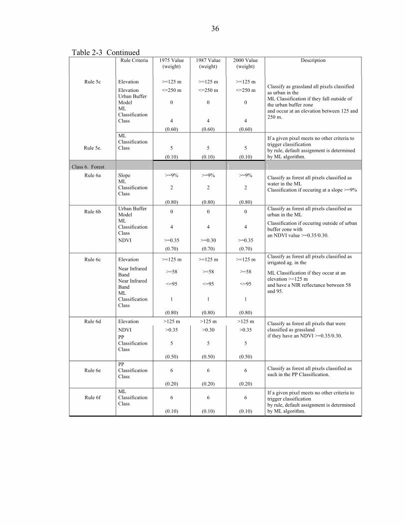
36

Table 2-3 Continued

Rule Criteria

1975 Value (weight)

1987 Value (weight)

2000 Value (weight)

Description

Rule 5c Elevation >=125 m >=125 m >=125 m Elevation <=250 m <=250 m <=250 m

Urban Buffer Model 0 0 0

ML Classification Class 4 4 4

(0.60) (0.60) (0.60)

Classify as grassland all pixels classified as urban in the ML Classification if they fall outside of the urban buffer zone and occur at an elevation between 125 and 250 m.

Rule 5e.

ML Classification Class 5 5 5

(0.10) (0.10) (0.10)

If a given pixel meets no other criteria to trigger classification by rule, default assignment is determined by ML algorithm.

Class 6. Forest Rule 6a Slope >=9% >=9% >=9%

ML Classification Class

2 2 2

(0.80) (0.80) (0.80)

Classify as forest all pixels classified as water in the ML Classification if occuring at a slope >=9%

Rule 6b Urban Buffer Model 0 0 0 Classify as forest all pixels classified as

urban in the ML

ML Classification Class

4 4 4

NDVI >=0.35 >=0.30 >=0.35 (0.70) (0.70) (0.70)

Classification if occuring outside of urban buffer zone with an NDVI value >=0.35/0.30.

Rule 6c Elevation >=125 m >=125 m >=125 m Classify as forest all pixels classified as irrigated ag. in the

Near Infrared Band >=58 >=58 >=58

Near Infrared Band <=95 <=95 <=95

ML Classification Class

1 1 1

(0.80) (0.80) (0.80)

ML Classification if they occur at an elevation >=125 m and have a NIR reflectance between 58 and 95.

Rule 6d Elevation >125 m >125 m >125 m NDVI >0.35 >0.30 >0.35

PP Classification Class

5 5 5

(0.50) (0.50) (0.50)

Classify as forest all pixels that were classified as grassland if they have an NDVI >=0.35/0.30.

Rule 6e PP Classification Class

6 6 6

(0.20) (0.20) (0.20)

Classify as forest all pixels classified as such in the PP Classification.

Rule 6f ML Classification Class

6 6 6

(0.10) (0.10) (0.10)

If a given pixel meets no other criteria to trigger classification by rule, default assignment is determined by ML algorithm.

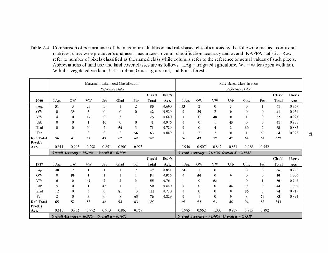
Table 2-4. Comparison of performance of the maximum likelihood and rule-based classifications by the following means: confusion matrices, class-wise producer’s and user’s accuracies, overall classification accuracy and overall KAPPA statistic. Rows refer to number of pixels classified as the named class while columns refer to the reference or actual values of such pixels. Abbreviations of land use and land cover classes are as follows: I.Ag = irrigated agriculture, Wa = water (open wetland), Wtlnd = vegetated wetland, Urb = urban, Glnd = grassland, and For = forest.

37

Maximum Likelihood Classification Rule-Based Classification Reference Data Reference Data:

Clas'd User's Clas'd User's2000 I.Ag. OW VW Urb Glnd For Total Acc. I.Ag. OW VW Urb Glnd For Total Acc.I.Ag. 51 3 23 5 1 2 85 0.600 53 2 0 5 0 1 61 0.869 OW 0 39 3 0 0 0 42 0.929 0 39 2 0 0 0 41 0.951 VW 4 0 17 0 3 1 25 0.680 3 0 48 0 1 0 52 0.923 Urb 0 0 1 40 0 0 41 0.976 0 0 1 40 0 0 41 0.976 Glnd 0 0 10 2 56 3 71 0.789 0 0 4 2 60 2 68 0.882 For 1 1 3 0 2 56 63 0.889 0 2 2 0 1 59 64 0.922

Ref. Total 56 43 57 47 62 62 327 56 43 57 47 62 62 327 Prod.'s Acc. 0.911 0.907 0.298 0.851 0.903 0.903 0.946 0.907 0.842 0.851 0.968 0.952 Overall Accuracy = 79.20% Overall K = 0.7493 Overall Accuracy = 91.44% Overall K = 0.8935

Clas'd User's Clas'd User's1987 I.Ag. OW VW Urb Glnd For Total Acc. I.Ag. OW VW Urb Glnd For Total Acc.I.Ag. 40 2 1 1 1 2 47 0.851 64 1 0 1 0 0 66 0.970 OW 0 50 1 1 1 1 54 0.926 0 50 0 0 0 0 50 1.000 VW 6 0 42 2 2 3 55 0.764 1 0 53 1 0 1 56 0.946 Urb 5 0 1 42 1 1 50 0.840 0 0 0 44 0 0 44 1.000 Glnd 12 0 5 0 81 13 111 0.730 0 0 0 0 86 8 94 0.915 For 2 0 3 0 8 63 76 0.829 0 1 0 0 8 74 83 0.892

Ref. Total 65 52 53 46 94 83 393 65 52 53 46 94 83 393 Prod.'s Acc. 0.615 0.962 0.792 0.913 0.862 0.759 0.985 0.962 1.000 0.957 0.915 0.892 Overall Accuracy = 80.92% Overall K = 0.7672 Overall Accuracy = 94.40% Overall K = 0.9318

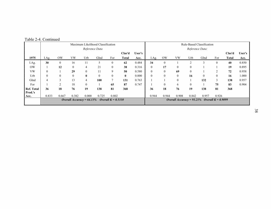
Table 2-4. Continued

38

Maximum Likelihood Classification Rule-Based Classification Reference Data Reference Data:

Clas'd User's Clas'd User's1975 I.Ag. OW VW Urb Glnd For Total Acc. I.Ag. OW VW Urb Glnd For Total Acc.I.Ag. 30 0 16 11 5 0 62 0.484 34 0 1 2 3 0 40 0.850 OW 1 12 0 4 21 0 38 0.316 0 17 0 0 1 1 19 0.895 VW 0 1 29 0 11 9 50 0.580 0 0 69 0 1 2 72 0.958 Urb 0 0 0 0 0 0 0 0.000 0 0 0 16 0 0 16 1.000 Glnd 4 3 13 4 100 7 131 0.763 1 1 0 1 132 3 138 0.957 For 1 2 18 0 1 65 87 0.747 1 0 6 0 1 75 83 0.904

Ref. Total 36 18 76 19 138 81 368 36 18 76 19 138 81 368 Prod.'s Acc. 0.833 0.667 0.382 0.000 0.725 0.802 0.944 0.944 0.908 0.842 0.957 0.926

Overall Accuracy = 64.13% Overall K = 0.5310

Overall Accuracy = 93.21% Overall K = 0.9099

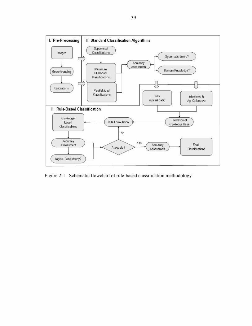
39

Figure 2-1. Schematic flowchart of rule-based classification methodology

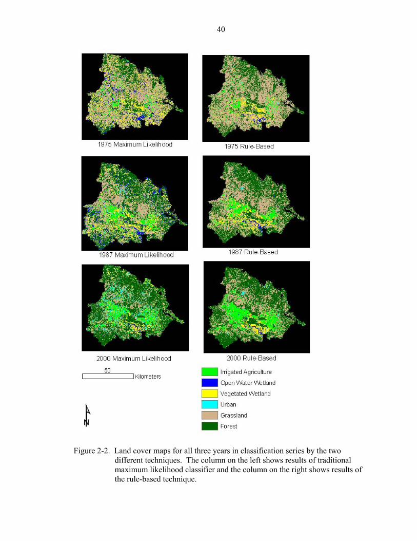
40

Figure 2-2. Land cover maps for all three years in classification series by the two

different techniques. The column on the left shows results of traditional maximum likelihood classifier and the column on the right shows results of the rule-based technique.

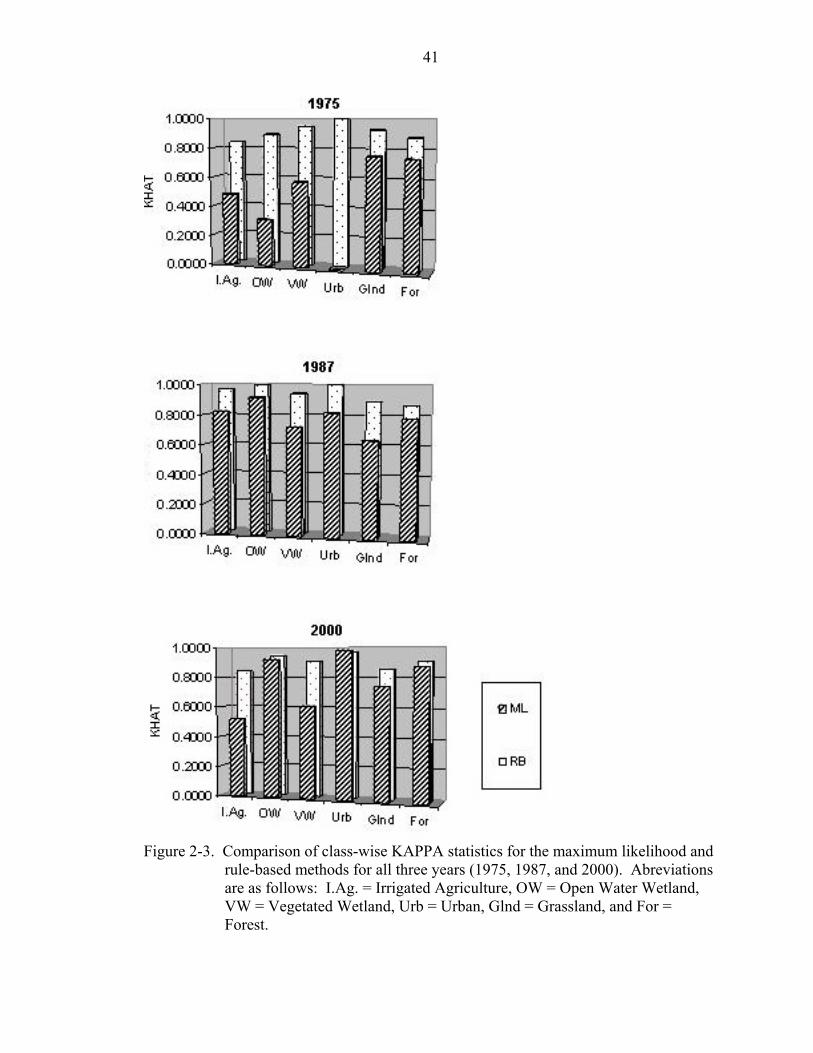
41

Figure 2-3. Comparison of class-wise KAPPA statistics for the maximum likelihood and

rule-based methods for all three years (1975, 1987, and 2000). Abreviations are as follows: I.Ag. = Irrigated Agriculture, OW = Open Water Wetland, VW = Vegetated Wetland, Urb = Urban, Glnd = Grassland, and For = Forest.

CHAPTER 3 LANDCOVER DYNAMICS IN THE TEMPISQUE RIVER BASIN: PALO VERDE

NATIONAL PARK IN THE WATERSHED CONTEXT

Introduction

The concept of protected area management has provoked a contentious and long-

standing debate in both the biological and social sciences (e.g., Terborgh1997, Bhagwat et

al. 2001, Bruner et al. 2001, Wilshusen et al. 2001). Overall efficacy of protected area

management for the conservation of biodiversity is still largely unclear. This is, perhaps, in

part due to different notions about what criteria constitute success with regard to

conservation goals. Also, because protected areas reside in dynamic landscapes, their

‘effectiveness’ changes over time and space in ways that have yet to be sufficiently

addressed. Narrowing the degree of uncertainty on the performance of protected areas in

achieving defined conservation goals is increasingly important and has exaggerated

implications in tropical environments where much of global biodiversity and provision of

environmental services like carbon sequestration occur.

One approach to assess the effectiveness of protected area management is to examine

its impact on land cover patterns and conversion processes since the time of park

establishment. Effectively managed reserves are expected to conserve and/or promote the

regeneration of “natural” land-cover types. Changes in land cover may result directly from

land use activities occurring within park bounds. Alternatively, land-cover changes may

occur as an indirect effect from activities physically removed from the park but which are

manifested within its bounds. The dynamic nature of land cover patterns and changes is a

42

43

multi-scale phenomenon that affects ecological attributes like trophic interactions, species

composition and dispersal, carbon sequestration, climatic patterns and water balance

(Kepner 2000). Land cover data are thus an essential tool, despite their coarse ‘ecological

resolution,’ for assessing the state of protected areas. These data can, in turn, inform and

direct finer analyses of the changing ecology within protected areas.

A modest but expanding body of literature addresses the issue of land-cover change

in relation to the effectiveness of protected areas as a general management regimes. Bruner

et al. (2001) surveyed park officials for 93 protected areas throughout the tropics to assess

the degree to which parks effectively prevented land clearing, amongst other threats.

Along similar lines, Rao et al. (2002) conducted site visits to 20 protected areas in

Myanmar to determine the nature and level of occurrences of incompatible land and

resource use. More commonly, researchers have used satellite-based land cover data to

compare rates of deforestation and degree of forest patch fragmentation within parks and

their surroundings (Sanchez-Azofeifa et al. 1999, Sanchez-Azofeifa et al. 2002,

Southworth et al. 2004). The explicitly spatial design of biosphere reserves with their

characteristic cores and buffers has also been evaluated with remotely sensed data in terms

of preventing deforestation (Hayes et al. 2002) and ‘natural area’ conversion (Walker and

Solecki 1999).

While this body of work provides valuable insights into the issues surrounding

protected area management, case studies that document land-cover change (LCC) within

established protected areas since the time of their establishment are still scarce. This

scarcity is particularly true for higher levels of taxonomic resolution in land-cover

classification schemes. As an illustration, all of the aforementioned evaluations of land-

44

cover change in protected areas employ a dichotomous forest/non-forest classification.

Such simplification has been justified by the preeminence of deforestation as a major driver

of the global environmental change (Geist and Lambin 2002) and by the difficulty and

expense of obtaining greater taxonomic resolution (Langford and Bell 1997b, Mertens and

Lambin 2000, Daniels in prep.). However, in many landscapes dichotomous land cover

models eliminate, through land cover aggregation, important information about the patterns

and processes of LCC and its drivers. This may be particularly true for protected areas

where subtle land cover transitions are sometimes driven by processes less obvious than

those of the nonprotected landscape. Furthermore, non-forest land covers, like wetlands,

may comprise a smaller extent of the landscape but are critical for ecological services and

regulation of regional environmental processes (Sparks 1995).

Criteria and guidelines for reserve site selection, design and management approaches

using concepts from landscape ecology and island biogeography theory have been treated

extensively in the literature (e.g.,, Arnold 1995, Primack 1993, Schwartz 1999, Sanderson

et al. 2002). These concepts are largely drawn from theoretical models on habitat

connectivity and minimum dynamic area for foci species and ecological processes (Pickett

and Thompson 1978), however, rather than based on empirical data. As a possible result,

the position of protected areas in their watersheds is one critical factor virtually ignored in

the literature on reserve design, selection and management (Pringle 2001). Understanding

the water balance characteristics and over-land surface flows in the area surrounding the

park and vice versa is critical but largely overlooked. Understanding of hydrologic

function and its implications at the landscape level and beyond is nascent (Pringle 2003,

Vorosmarty 2002) and thus incorporating park management into its respective hydroscape

45

poses even greater challenges. Watersheds provide natural, hierarchical units within which

park function can be conceptualized and studied, particularly if greater detail in land cover

and land use can be achieved.

In essence, park boundaries are arbitrarily-drawn political lines while the geographic

area defined as a park fits into a complex, dynamic, biophysical and land-use matrix that

must be recognized and understood (Poiani et al. 2000). Even optimally functioning and

connected reserve networks per se are likely to support but a mere fraction of the

biodiversity and ecological services we seek to preserve. Nonetheless, opportunities for

creative land use configurations, conservation policies and scenario planning that

complement reserve function are possible if the ecological values and threats of the

surrounding biophysical and socioeconomic matrix are considered (Harvey and Haber

1999, Daily et al. 2003).

Historic and current land use patterns and population settlement at the time of reserve

establishment are often the primary factors affecting the ways in which parks sites are

selected, established and managed (Runte 1979, Hunter and Yonzon 1993, Pressey 1994).

Rivard et al. (1999) found land use patterns in Canada’s national parks to be highly

correlated with patterns surrounding the parks. Similarly, both species richness and

extirpations were more highly correlated with regional characteristics than to those of the

parks in which they occurred. The extinction of large mammals in western U.S. parks was

found to correlate significantly with surrounding human density, but surprisingly enough,

not with park area (Parks and Harcourt 2001). And finally, many common agriculture-

related land-management systems are known to affect both land cover dynamics and

ecological processes at scales beyond their actual temporal and spatial extents (Shankman

46

1996, Lemly 2000). All of these factors underscore the need to move away from merely

theoretical models of park design and function to consider the unique context of each

protected area for the determination of best integrated management practices.

This research presents a case study of protected area management in the watershed

context for Palo Verde National Park (PVNP) in Guanacaste, Costa Rica. This site was

chosen because of its unique mosaic of habitat types. Also, by virtue of its position at the

bottom of a large drainage basin, this park serves as an instructive case study of the role of

hydrologic connectivity between parks and their host watersheds. The watershed

surrounding PVNP has undergone drastic landscape transformation in the past 25 years and

thus the region provides an appropriate context for exploring the effect of protected area

management on land cover transition. Specifically, I address the following questions: (1)

How have land use and land-cover changed in the Tempisque River Basin and Palo Verde

National Park over the last 25 years? and (2) What is the effect of Palo Verde National

Park on land-cover change given the watershed context? By watershed context I refer to

the historic and current land-management systems, their implications for land cover

dynamics, and the ways in which the biophysical and social structure of the landscape

either constrains or facilitates certain land cover conversions.

Regional Context

Study Region Description

The Tempisque River Watershed is in the northwestern province of Guanacaste with

an extent of 5,404 km2 (Figure 3-1), or 10 % of the national area. The watershed has a

mean temperature of 27.5oC and mean annual precipitation of 1817 mm falling between

May and November (Mateo-Varga 2001). Mean precipitation between May and November

is about the same throughout the watershed. There is more variability during the dry

47

season, however, with the lower, western watershed receiving 0 mm of precipitation on

average, while higher elevation areas on the cordillera receive around 61 mm on average.

The River runs generally north to south through the center of the basin, increasing in

volume in the southern watershed with the confluence of the eastern originating Bebedero

River and several important tributaries. Thirteen different Holdridge life zones are found

in the watershed (Holdridge 1967) with myriad habitats including tropical dry forest, moist

pre-montane forest and vast seasonal wetlands. The eastern border of the watershed is

defined by the Guanacaste Mountain Range that reaches over 2000 m elevation. The

Tempisque River experiences semiannual floods thus making it one of Central America’s

more productive regions and the only part of lowland Costa Rica to be continuously

inhabited since the beginning of the colonial era (Peters 2001).

Historical Context for Transformation in the Tempisque Watershed

Since the arrival of the Spanish, the landscape has been historically dominated by

cattle ranching and low-intensity or subsistence agriculture of beans, maize, sorghum and

indigo. In this region, beef cattle ranching proved more profitable than in other parts of the

country (SEPSA in Harrison 1991). However, high capital investment was required to

maintain sufficient feed during the dry season. Alternatively, green wetland areas of the

lowlands or cloud-bathed pasture areas high on the cordillera provided ample grazing

potential during the dry season. These constraints of the biophysical landscape in relation

to the dominant economic activity probably contributed to the region’s characteristically

large landholdings and low population density, which even today equals less than 31

people per square kilometer (CCT 1998). With the construction of the Panamerican

Highway in the 1950s, slight intensification and a shift in crop cultivation occurred with

the increased production of sugar cane, cotton and sorghum for the national and

48

international markets. Cattle ranching remained, however, the defining social and

economic feature of the landscape.

Several conditions aligned at multiple economic and political scales, setting the stage

for the transformation seen by the Tempisque River landscape beginning in the mid-1970s

(Figure 3-2). When the beef market precipitously declined in the 1970s, Costa Rica was

the 4th largest supplier of beef to the United States (Peters 2001) and had one of the highest

per capita debt loads anywhere in the developing world (Biesanz et al. 1982). This

economic shock was followed by the global economic downturn (DeWitt 1977) and the

ensuing national financial crisis of 1980 in which Costa Rica defaulted on international

loans (Lara 1995). Implications were grave for Costa Rica as a nation, but particularly for

the land-management regime that had sustained the Tempisque Basin for nearly five

hundred years (Martinez 2000).

After the crisis of 1980, economic and structural adjustments proceeded at the behest

of international lending institutions. Included in Costa Rica’s strategies for economic

recovery and development were increased emphases on development of energy resources

and investment in the budding ecotourism industry, both of which would directly and

indirectly decrease dependence on petroleum imports from oil to fertilizer. In the

Tempisque Basin these strategies were manifested in tangible ways with development and

conservation works-in-progress that assumed greater import after the economic crisis. The

works-in-progress included the Arenal-Tempisque Irrigation Project (PRAT or Proyecto

Riego Arenal Tempisque) and conservation of the area that later became PVNP. Both

projects entailed changes in the spatiotemporal patterns of resource and land use, albeit at

opposite ends of the spectrum (Figure 3-2).

49

The concept of PRAT was born in the 1950s, but construction for the $50.5 million

dollar project (DeWitt 1977) came to fruition in the mid-1970s with financing from the

Inter-American Development Bank (IDB). The PRAT irrigation program forms part of a

larger hydroelectric project that generates the bulk of Costa Rica’s energy. In 1978, PRAT

dammed a formerly Caribbean-draining river to form Lago Arenal with a volume of 1570

million m3 and electric potential of 25,450 Mw per year. After generation of power at three

drops along the Pacific slopes, PRAT channels water to the lowlands of the Tempisque

Basin via some 234 km of canals whose average wet and dry season flow volumes are

around 45 m3/s and 62 m3/s respectively. The government purchased land on the eastern

side of the Tempisque that was subdivided into 5 ha lots for flooded rice cultivation and

distributed at subsidized rates to farmers. Otherwise, irrigation water went to existing

agroindustry operations who also extract water from the Tempisque River for irrigation (as

is the case for much of the cultivated area in the western half of the basin, beyond the reach

of PRAT). The project has taken over twenty years to fully implement and additional canal

networks may be built in the future.

Protected Areas in Costa Rica

Costa Rica is now well-known for its virtually unmatched system of protected areas.

This system forms a keystone component of the ecotourism industry that provides the

country’s largest source of foreign income. Since the national park service’s foundation in

1970, nearly 25% of the country’s national area has been placed under varying forms of

protection. This conservation system is now valued at over $1.2 billion dollars (Umana

1996). The park system is based largely upon the North American caretaker and people-

exclusion model. Palo Verde National Park was designated as a national park in 1990 but

nearly its full extent had been protected in two separate reserves since 1977. Prior to the

50

decree of any form of protection, the land was part of a large cattle ranch, Rancho

Comelco, that stretched from the floodplains up toward the cordillera (Gill 1988).

Palo Verde covers over 18,760 ha and protects a diverse mosaic of habitats. The park

includes the world’s most endangered habitat type, tropical dry forest, for which less than

two percent of the original extent along the Pacific slopes of the Central American-

Mexican isthmus remains (Janzen 1988). Over a third of PVNP is composed of a wetland

mosaic that historically provided critical habitat for migratory waterfowl. For this reason,

the site was given RAMSAR protection in 1991 (Mateo-Varga 2001). In addition to

attracting ecotourists, the Organization for Tropical Studies’ research station housed within

the park’s bounds serves as an important attractant for academic tourism.

Other national parks partially located in the basin include those of Barra Honda,

Rincon de la Vieja, Guanacaste and Santa Rosa. While lesser levels of protection and

management also exist within the watershed, such as Diria National Forest, the Lomas

Barbudal Reserve and private tracts of forest subsidized by the national government’s

environmental service payments program (PSA, 1996 Ley Forestal 7575), these areas

comprise 1.16% of the basin and have only more recently been established.

Methods

Land-cover classification

Four Landsat images were obtained to represent baseline land cover data and two

time steps thereafter. The first two images used to create a mosaic of the study region were

Landsat Multispectral Scanner (MSS) images from 1974 and 1975. The middle time point

was a Thematic Mapper (TM) image from 1987 and the final image was from the

Enhanced Thematic Mapper (ETM) platform for the year 2000. All images used were

from early in the dry season to facilitate identification of irrigated agriculture as a land use

51

category. Geometric rectification was performed using a nearest neighbor resampling

algorithm on the year 2000 image using ground control points taken in the field with GPS

to achieve a root mean square (RMS) error below 0.5 or 15 m. The later images were then

registered to this image and an overlay function was performed to ensure exact geographic

correspondence for the extent of the watershed. To ensure that differences in satellite data

across the series corresponded to changes on the ground, rather than differences at the

sensor level, all images underwent radiometric calibration, atmospheric corrections and

then radiometric rectification procedures. These processes eliminated sensor bias and

differences due to variations in solar angle (Jensen 1996). After calibration procedures, all

images were subset to the extent of the watershed for ease of processing and storage.

Training samples for the 2000 classification were collected during fieldwork in 2001.

Historic photo-mosaics corresponding to the dates of the older satellite imagery were used

to collect training samples for the 1974-75 mosaic and the 1987 image. Additionally, over

29 semi-structured land use/land history interviews were conducted throughout the

watershed to inform agricultural calendars, verify image interpretation and better

understand systems of land use over the study period. Land use and land cover classes

employed were irrigated agriculture, water/open wetland, vegetated wetland, urban,

grassland and forest (Table 3-1). Images were independently classified using a rule-based

approach that incorporated domain knowledge. Overall classification accuracy exceeded

90% for each date and class-wise accuracy matched or exceeded 85% for each date. For

details on the rule-based classification methodology see Daniels in prep.

Land-cover change Analysis: Spatially Implicit and Spatially Explicit

To ensure that the same extent of area was considered in each land cover map, areas

of cloud cover for any single date were eliminated from all others. The final outer

52

boundary of the 1974-1975 mosaic was used to define the final extent of the watershed

considered in this study. This method occurred because the oldest Landsat images in the

series were based on the first World Reference System (WRS 1) where the image footprint

cut off a triangular area of 110 km2 at the northern border of the watershed. The portions

of Santa Rosa, Guanacaste and Rincon de la Vieja National Parks that fall within the

watershed were eliminated in this process of eliminating clouds and image footprint

differences. And finally, to control for the evaluation of Palo Verde National Park alone,

the remaining tracks of protected lands of lesser degrees, comprising only 1.16% of the

original area of the basin, were not included in land cover evaluations since the imagery

series did not adequately represent the effect of management activities on land cover since

protection was decreed. These adjustments resulted in a total area of 5153 km2 or 95.35%

of the true extent of the basin used for this evaluation.

Land cover composition was then assessed for each land cover map (spatially

implicit) in the classification series to determine trends of net area change across the study

period for protected and nonprotected regions respectively (e.g., net increase in forest cover

in both regions; net decrease in wetland area for the nonprotected and net increase in

wetland area for the park). The net trends identified for each land cover class for the park

and nonprotected parts of the landscape were used to guide the spatially explicit analysis of

land cover conversion sequences.

The analysis was completed through the creation of a single raster surface

representing land cover trajectories or conversion sequences over the three dates by

recoding every possible combination of original land cover classes from all three years to a

unique value. For example, a single pixel followed over the three original land cover maps

53

may have transitioned from forest to grassland to irrigated agriculture. The unique value

assigned after recoding would reflect this trajectory. The relationship between land cover

classes and trajectories (Petit et al. 2001) is

mt = mtc

with mt being the total number of possible trajectories and mc the number of land cover

classes in the single date land cover maps. Finally t is number of images in the time series.

Although the single date images classified urban land use, its extent comprised such a

negligible portion of the landscape that it was not included in the trajectory analysis.

Accordingly, for this analysis, a total of mt = 53 = 125 trajectories were possible (versus

216 if urban had been included).

Determining Dominant Explanatory Trajectories

Because of the large number of possible trajectories in a three-image time series,

analyzing spatially explicit patterns of LCC in relation to the overall biophysical landscape

and protection status proved to be difficult. Thus, this research developed a set of rules to

determine the trajectories that reveal the most important land-cover change trends in the

watershed and simplify the LCC model into something that could be easily interpreted. If

the net area change for a given land cover was positive over the study period, trajectories

were examined in a backwards” manner to understand which land cover transitions explain

the increase. For example, for an increase in land cover X, the areas of all possible

trajectories ending in X (hereafter referred to as explanatory trajectories) for the final year

in the series were compared. In contrast, if the net area change for a given land cover was

negative over the study period, the trajectories were examined in a “forward” fashion to

understand what land cover transitions explain that decrease. For example, if a decrease in

54

land cover Y was observed over the study period, all possible explanatory trajectories

starting in Y for the first year of the time series were compared.

In the analysis of each land cover’s net-area trend, explanatory trajectories were

retained for further analysis up to the point where 80% of the net area change had been

accounted for or the point at which a given trajectory explained less than one percent of the

net-area trend, whichever occurred first. While it may appear that valuable information is

being omitted from the analysis, two important factors must be considered. The first factor

is that a classification error up to 10% exists within each single date classification and this

error is propagated across the land cover trajectories. The cutoff rules are justified in two

ways: (1) Explaining 80% of the net-area trend is sufficient to understand dominant

processes of land cover conversion for a given class and (2) Any trajectory explaining less

than one percent of the net-area trend observed is likely an amalgam of classification

errors. The second factor is that, as mentioned, the LCC model has extremely limited

interpretability for a multi-class change study without such simplification.

After identifying the dominant explanatory trajectories (i.e., those that met the cutoff

criteria) for each net area gain or loss in land cover across the study period, another round

of simplification occurred prior to analyzing how the dominant trajectories relate to the

overall biophysical and built landscape structure. Only trajectories with two land-cover

types showing change in a unidirectional fashion were retained. The idea was to reduce

error in the trajectories examined and also provide greater interpretability and

manageability in understanding how trajectories relate to the biophysical and built structure

of the landscape.

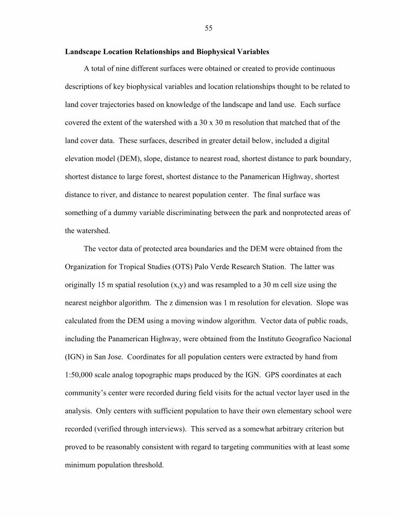
55

Landscape Location Relationships and Biophysical Variables

A total of nine different surfaces were obtained or created to provide continuous

descriptions of key biophysical variables and location relationships thought to be related to

land cover trajectories based on knowledge of the landscape and land use. Each surface

covered the extent of the watershed with a 30 x 30 m resolution that matched that of the

land cover data. These surfaces, described in greater detail below, included a digital

elevation model (DEM), slope, distance to nearest road, shortest distance to park boundary,

shortest distance to large forest, shortest distance to the Panamerican Highway, shortest

distance to river, and distance to nearest population center. The final surface was

something of a dummy variable discriminating between the park and nonprotected areas of

the watershed.

The vector data of protected area boundaries and the DEM were obtained from the

Organization for Tropical Studies (OTS) Palo Verde Research Station. The latter was

originally 15 m spatial resolution (x,y) and was resampled to a 30 m cell size using the

nearest neighbor algorithm. The z dimension was 1 m resolution for elevation. Slope was

calculated from the DEM using a moving window algorithm. Vector data of public roads,

including the Panamerican Highway, were obtained from the Instituto Geografico Nacional

(IGN) in San Jose. Coordinates for all population centers were extracted by hand from

1:50,000 scale analog topographic maps produced by the IGN. GPS coordinates at each

community’s center were recorded during field visits for the actual vector layer used in the

analysis. Only centers with sufficient population to have their own elementary school were

recorded (verified through interviews). This served as a somewhat arbitrary criterion but

proved to be reasonably consistent with regard to targeting communities with at least some

minimum population threshold.

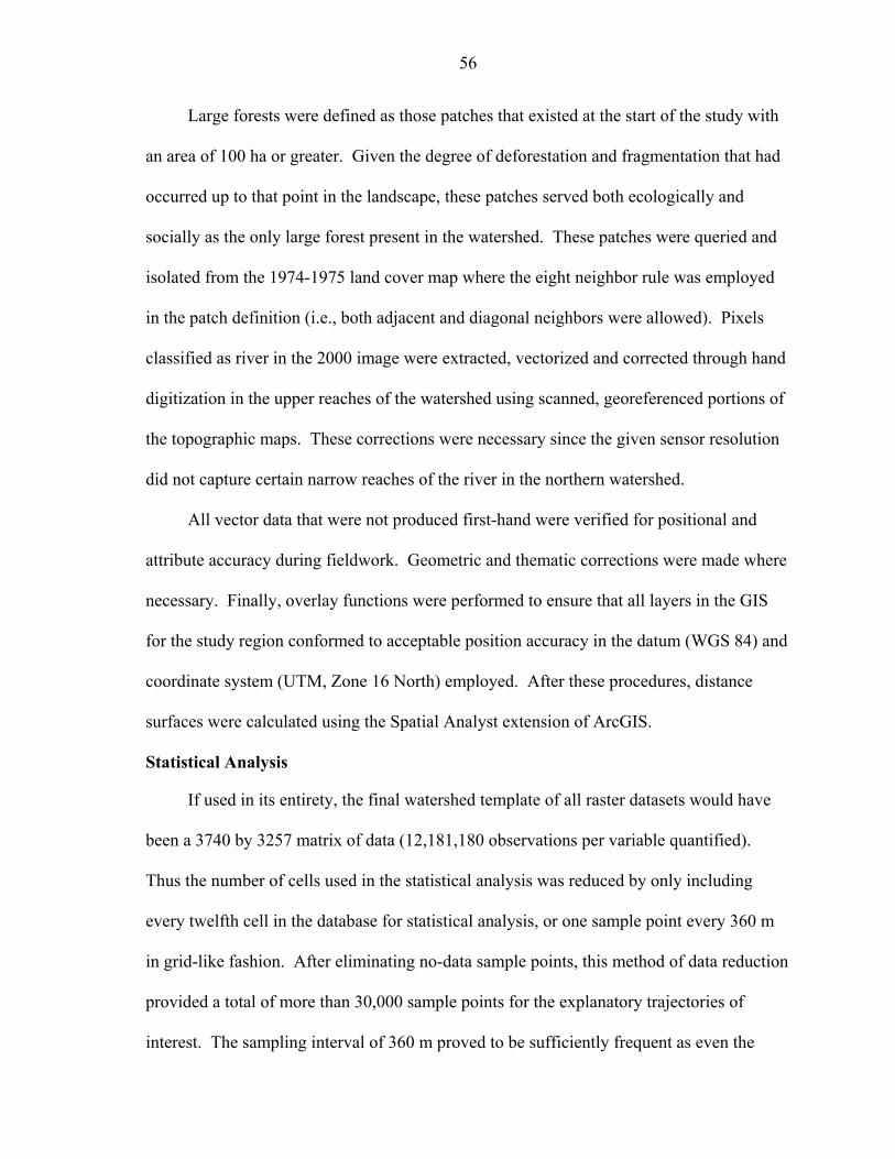
56

Large forests were defined as those patches that existed at the start of the study with

an area of 100 ha or greater. Given the degree of deforestation and fragmentation that had

occurred up to that point in the landscape, these patches served both ecologically and

socially as the only large forest present in the watershed. These patches were queried and

isolated from the 1974-1975 land cover map where the eight neighbor rule was employed

in the patch definition (i.e., both adjacent and diagonal neighbors were allowed). Pixels

classified as river in the 2000 image were extracted, vectorized and corrected through hand

digitization in the upper reaches of the watershed using scanned, georeferenced portions of

the topographic maps. These corrections were necessary since the given sensor resolution

did not capture certain narrow reaches of the river in the northern watershed.

All vector data that were not produced first-hand were verified for positional and

attribute accuracy during fieldwork. Geometric and thematic corrections were made where

necessary. Finally, overlay functions were performed to ensure that all layers in the GIS

for the study region conformed to acceptable position accuracy in the datum (WGS 84) and

coordinate system (UTM, Zone 16 North) employed. After these procedures, distance

surfaces were calculated using the Spatial Analyst extension of ArcGIS.

Statistical Analysis

If used in its entirety, the final watershed template of all raster datasets would have

been a 3740 by 3257 matrix of data (12,181,180 observations per variable quantified).

Thus the number of cells used in the statistical analysis was reduced by only including

every twelfth cell in the database for statistical analysis, or one sample point every 360 m

in grid-like fashion. After eliminating no-data sample points, this method of data reduction

provided a total of more than 30,000 sample points for the explanatory trajectories of

interest. The sampling interval of 360 m proved to be sufficiently frequent as even the

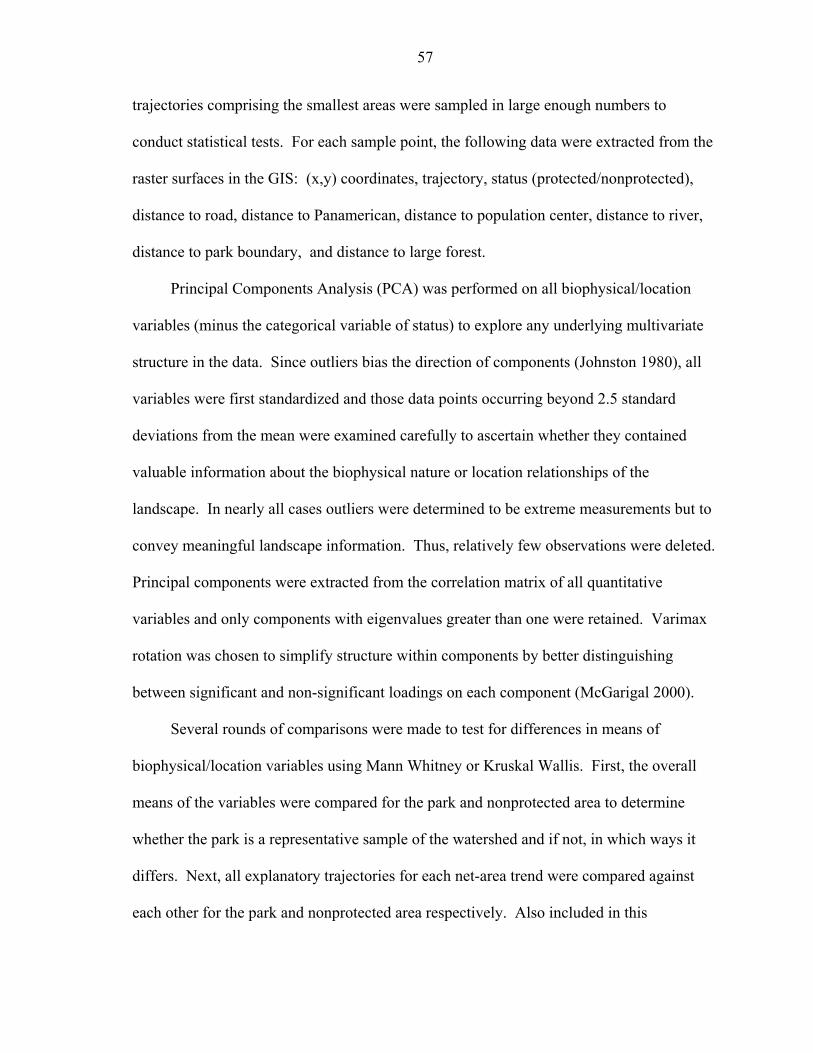
57

trajectories comprising the smallest areas were sampled in large enough numbers to

conduct statistical tests. For each sample point, the following data were extracted from the

raster surfaces in the GIS: (x,y) coordinates, trajectory, status (protected/nonprotected),

distance to road, distance to Panamerican, distance to population center, distance to river,

distance to park boundary, and distance to large forest.

Principal Components Analysis (PCA) was performed on all biophysical/location

variables (minus the categorical variable of status) to explore any underlying multivariate

structure in the data. Since outliers bias the direction of components (Johnston 1980), all

variables were first standardized and those data points occurring beyond 2.5 standard

deviations from the mean were examined carefully to ascertain whether they contained

valuable information about the biophysical nature or location relationships of the

landscape. In nearly all cases outliers were determined to be extreme measurements but to

convey meaningful landscape information. Thus, relatively few observations were deleted.

Principal components were extracted from the correlation matrix of all quantitative

variables and only components with eigenvalues greater than one were retained. Varimax

rotation was chosen to simplify structure within components by better distinguishing

between significant and non-significant loadings on each component (McGarigal 2000).

Several rounds of comparisons were made to test for differences in means of

biophysical/location variables using Mann Whitney or Kruskal Wallis. First, the overall

means of the variables were compared for the park and nonprotected area to determine

whether the park is a representative sample of the watershed and if not, in which ways it

differs. Next, all explanatory trajectories for each net-area trend were compared against

each other for the park and nonprotected area respectively. Also included in this

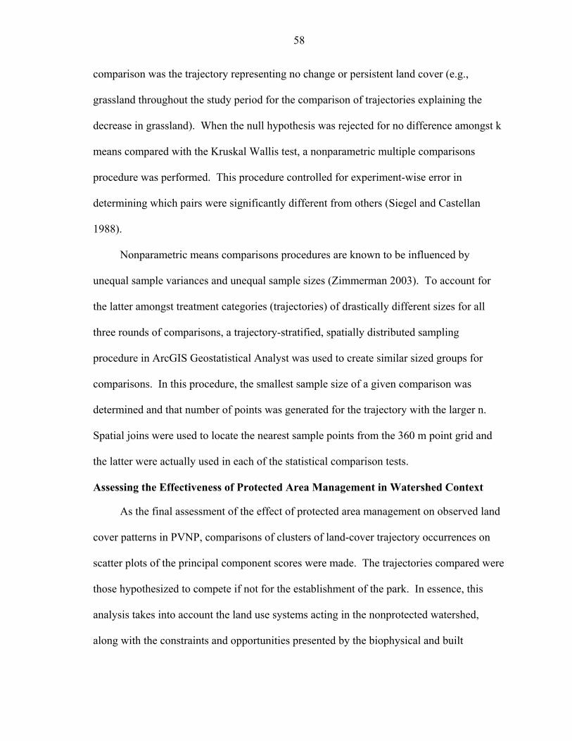
58

comparison was the trajectory representing no change or persistent land cover (e.g.,

grassland throughout the study period for the comparison of trajectories explaining the

decrease in grassland). When the null hypothesis was rejected for no difference amongst k

means compared with the Kruskal Wallis test, a nonparametric multiple comparisons

procedure was performed. This procedure controlled for experiment-wise error in

determining which pairs were significantly different from others (Siegel and Castellan

1988).

Nonparametric means comparisons procedures are known to be influenced by

unequal sample variances and unequal sample sizes (Zimmerman 2003). To account for

the latter amongst treatment categories (trajectories) of drastically different sizes for all

three rounds of comparisons, a trajectory-stratified, spatially distributed sampling

procedure in ArcGIS Geostatistical Analyst was used to create similar sized groups for

comparisons. In this procedure, the smallest sample size of a given comparison was

determined and that number of points was generated for the trajectory with the larger n.

Spatial joins were used to locate the nearest sample points from the 360 m point grid and

the latter were actually used in each of the statistical comparison tests.

Assessing the Effectiveness of Protected Area Management in Watershed Context

As the final assessment of the effect of protected area management on observed land

cover patterns in PVNP, comparisons of clusters of land-cover trajectory occurrences on

scatter plots of the principal component scores were made. The trajectories compared were

those hypothesized to compete if not for the establishment of the park. In essence, this

analysis takes into account the land use systems acting in the nonprotected watershed,

along with the constraints and opportunities presented by the biophysical and built

59

structure of the landscape, to give a better indication of the effect of protected area

management on land cover patterns.

Results and Discussion

Park versus Nonprotected Area

Comparison of biophysical and location relationships for the park and nonprotected

area, along with contrasting initial land cover conditions for the study period, reveal that

the park is not a representative sample of the landscape. This is often the case with

protected areas, as they often represent spots of elevated biodiversity that may be related to

unique juxtapositions of land forms and vegetation communities. Alternatively, protected

land may often be unproductive and/or inaccessible and thus, the only remaining ‘natural’

habitat in the landscape (Hunter and Yonzon 1993, Pressey 1994).

In the case of baseline data for PVNP relative to the surrounding watershed, the park

was found to have different land cover composition with 33% less grassland, nearly four

percent more forest cover, over seven percent more open water wetland, and over 26%

more vegetated wetlands (Table 3-2). Irrigated agriculture comprised almost five percent

of the nonprotected landscape at the beginning of the study period but was not present in

baseline data for the region that became the park.

With regard to the biophysical landscape and location relationships therein, the

protected and nonprotected regions differ considerably (Table 3-2). Means of all variables

were found to be significantly different (Mann Whitney, p<0.000). In short, the average 30

x 30 m raster cell in the park can be described as being lower in elevation, slightly gentler

in slope, closer to a large forest patch, closer to the park boundary and closer to the river.

Cells in the park are also more isolated than the average cell in the nonprotected landscape

60

as evidenced by larger distances from roads, the Panamerican Highway and population

centers.

Many of these differences in both land cover and biophysical/location variables are

functions of the park’s size relative to the nonprotected watershed and its position in the

landscape. Occurring as a small, low-lying area in the lower watershed along the river, the

park clearly integrates effects of activities in the upper watershed and is more affected by

its surroundings than vice versa. As a function of its location, the park is well-endowed

with wetlands that cover over one third of its area. In light of these facts, the small

difference in forest cover (four percent) between the protected and nonprotected regions

becomes more significant. Similarly, given that the wetlands occupy about one third of the

park and occur generally in the flattest areas along the river (less than two percent), the

7.71% mean slope represents appreciable relief (relative to the nonprotected mean that is

only about three percent higher). Most topography in the park is a result of limestone karst

structures that have dramatic slopes but reach an elevation of less than 200m. Because

upland areas were characterized by unsuitable slopes and wetland areas served as grazing

grounds for cattle, the park was more forested than its surroundings at the time of

establishment. Increased forest cover existed despite the area’s management by the same

dominant land use system as the rest of the watershed (cattle ranching).

Net Area Land-cover change: Park and Nonprotected Area

With only one exception, net area land-cover change occurs in a unidirectional

fashion, increasing or decreasing for each class across the three dates in the study period

(Figure 3-4). For both the park and nonprotected watershed, grassland decreased

dramatically (15% and 30% respectively) and forest cover increased substantially (about

20% each). It is important to note that relatively little area in the basin occurs naturally as

61

grassland. Natural grassland only occurs on certain volcanic slopes where both poor soil

structure and possible downwind, agriculture-related fire frequency prevents dominance of

woody growth. For this reason, grassland is a somewhat reliable proxy for pasture land use

in this landscape except when, due to soil compaction on heavily grazed pastures, woody

succession may not ensue even several years after the land ceases to be used as pasture

(Gillespie 2000, Gerhardt 1993).

Open water wetland decreased considerably in the park from eight percent to two

percent, while little change was observed in the nonprotected landscape. The latter is

probably true because the only considerable area of open water wetland in the nonprotected

landscape is the river itself. Also, losses in natural open wetlands of the floodplain are

masked in the land cover maps by the formation of several small dammed areas that are

part of the irrigation program.

Vegetated wetlands decreased in the nonprotected area by one half while a slight net

increase of about two percent was observed in the park. This fluctuation of vegetated

wetland area in the park from 1975 to 1987 and then 1987 to 2000 is likely related to the

warm and cold phases of El Nino Southern Oscillation (ENSO) respectively (Waylen and

Laporte 1999). The second image date, 1987, was a particularly dry year and some true,

functional wetland area may have been classified as grassland on that date. In the

nonprotected region, irrigated agriculture increased about three fold from less than five

percent of the landscape in 1975 to nearly 15% in 2000. Although a slight increase in

irrigated agriculture was observed, this land use comprised a mere 1.5% of the park in

2000. Based on personal communication with local officials, this increase of agricultural

land use within the park is a land tenure issue rather than an incursion issue that threatens

62

to move further into the park. In essence, different government ministries planned different

uses for the same parcels of land.

Figure 3-4a shows land-cover change in the nonprotected region of the watershed

across the dates of the study period. Reforestation can be observed mostly in the upper

watershed while increase in irrigated agriculture land use occurs in the lower watershed,

near the river. Loss of wetlands occurs as the floodplain area becomes increasingly filled

with irrigated agriculture fields. These maps reveal that the river itself forms the bulk of

open water wetlands in the nonprotected watershed.

Land-cover change for PVNP is shown in figure 4b. Similar to the nonprotected

region, reforestation is observed in the upland areas of the park. In the lowlands, some

interplay between grassland and vegetated wetlands can be observed. Also in this region,

the loss of open water wetlands is obvious. The small increase in irrigated agriculture

clearly occurs only along the northern border, corroborating the accounts of local officials.

Explaining Net Area Changes with Dominant Trajectories

The dominant trajectories explain the actual sequences of land cover transitions that

each of the five land covers moved from (in the case of net area decrease) or moved to (in

the case of net area increase). To reiterate, trajectories were retained for interpretation and

graphing up to one of two cutoff points, whichever occurred first: (1) the point where >

80% of change in an initial (in the case of net area decrease) or final (in the case of net area

increase) land cover had been explained or (2) the point where trajectories explained less

than one percent of the change of a given initial or final land cover.

Spatially explicit analysis of decrease in grasslands

In explaining the net area decrease for grasslands, seven trajectories were retained for

the nonprotected area and five for the park (Figure 6a). Both parts of the landscape show a

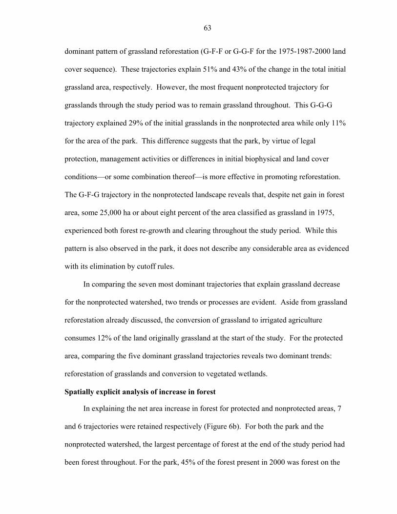
63

dominant pattern of grassland reforestation (G-F-F or G-G-F for the 1975-1987-2000 land

cover sequence). These trajectories explain 51% and 43% of the change in the total initial

grassland area, respectively. However, the most frequent nonprotected trajectory for

grasslands through the study period was to remain grassland throughout. This G-G-G

trajectory explained 29% of the initial grasslands in the nonprotected area while only 11%

for the area of the park. This difference suggests that the park, by virtue of legal

protection, management activities or differences in initial biophysical and land cover

conditions—or some combination thereof—is more effective in promoting reforestation.

The G-F-G trajectory in the nonprotected landscape reveals that, despite net gain in forest

area, some 25,000 ha or about eight percent of the area classified as grassland in 1975,

experienced both forest re-growth and clearing throughout the study period. While this

pattern is also observed in the park, it does not describe any considerable area as evidenced

with its elimination by cutoff rules.

In comparing the seven most dominant trajectories that explain grassland decrease

for the nonprotected watershed, two trends or processes are evident. Aside from grassland

reforestation already discussed, the conversion of grassland to irrigated agriculture

consumes 12% of the land originally grassland at the start of the study. For the protected

area, comparing the five dominant grassland trajectories reveals two dominant trends:

reforestation of grasslands and conversion to vegetated wetlands.

Spatially explicit analysis of increase in forest

In explaining the net area increase in forest for protected and nonprotected areas, 7

and 6 trajectories were retained respectively (Figure 6b). For both the park and the

nonprotected watershed, the largest percentage of forest at the end of the study period had

been forest throughout. For the park, 45% of the forest present in 2000 was forest on the

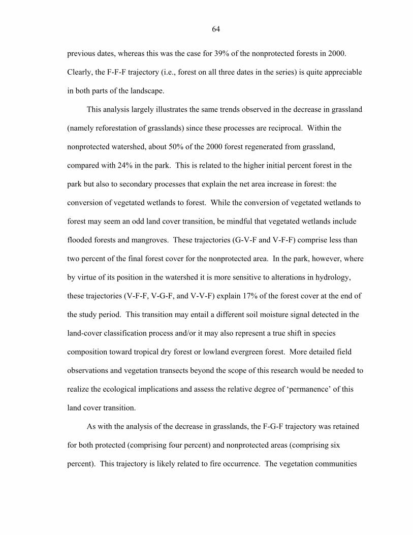
64

previous dates, whereas this was the case for 39% of the nonprotected forests in 2000.

Clearly, the F-F-F trajectory (i.e., forest on all three dates in the series) is quite appreciable

in both parts of the landscape.

This analysis largely illustrates the same trends observed in the decrease in grassland

(namely reforestation of grasslands) since these processes are reciprocal. Within the

nonprotected watershed, about 50% of the 2000 forest regenerated from grassland,

compared with 24% in the park. This is related to the higher initial percent forest in the

park but also to secondary processes that explain the net area increase in forest: the

conversion of vegetated wetlands to forest. While the conversion of vegetated wetlands to

forest may seem an odd land cover transition, be mindful that vegetated wetlands include

flooded forests and mangroves. These trajectories (G-V-F and V-F-F) comprise less than

two percent of the final forest cover for the nonprotected area. In the park, however, where

by virtue of its position in the watershed it is more sensitive to alterations in hydrology,

these trajectories (V-F-F, V-G-F, and V-V-F) explain 17% of the forest cover at the end of

the study period. This transition may entail a different soil moisture signal detected in the

land-cover classification process and/or it may also represent a true shift in species

composition toward tropical dry forest or lowland evergreen forest. More detailed field

observations and vegetation transects beyond the scope of this research would be needed to

realize the ecological implications and assess the relative degree of ‘permanence’ of this

land cover transition.

As with the analysis of the decrease in grasslands, the F-G-F trajectory was retained

for both protected (comprising four percent) and nonprotected areas (comprising six

percent). This trajectory is likely related to fire occurrence. The vegetation communities

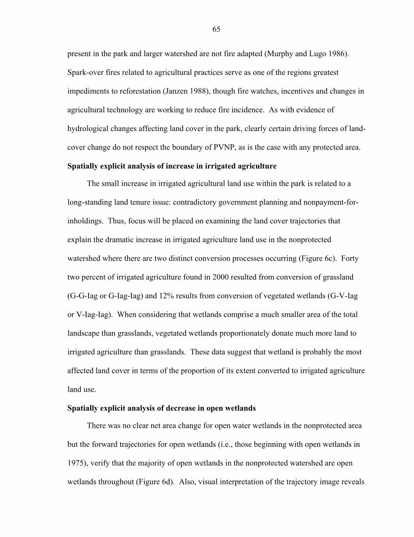
65

present in the park and larger watershed are not fire adapted (Murphy and Lugo 1986).

Spark-over fires related to agricultural practices serve as one of the regions greatest

impediments to reforestation (Janzen 1988), though fire watches, incentives and changes in

agricultural technology are working to reduce fire incidence. As with evidence of

hydrological changes affecting land cover in the park, clearly certain driving forces of land-

cover change do not respect the boundary of PVNP, as is the case with any protected area.

Spatially explicit analysis of increase in irrigated agriculture

The small increase in irrigated agricultural land use within the park is related to a

long-standing land tenure issue: contradictory government planning and nonpayment-for-

inholdings. Thus, focus will be placed on examining the land cover trajectories that

explain the dramatic increase in irrigated agriculture land use in the nonprotected

watershed where there are two distinct conversion processes occurring (Figure 6c). Forty

two percent of irrigated agriculture found in 2000 resulted from conversion of grassland

(G-G-Iag or G-Iag-Iag) and 12% results from conversion of vegetated wetlands (G-V-Iag

or V-Iag-Iag). When considering that wetlands comprise a much smaller area of the total

landscape than grasslands, vegetated wetlands proportionately donate much more land to

irrigated agriculture than grasslands. These data suggest that wetland is probably the most

affected land cover in terms of the proportion of its extent converted to irrigated agriculture

land use.

Spatially explicit analysis of decrease in open wetlands

There was no clear net area change for open water wetlands in the nonprotected area

but the forward trajectories for open wetlands (i.e., those beginning with open wetlands in

1975), verify that the majority of open wetlands in the nonprotected watershed are open

wetlands throughout (Figure 6d). Also, visual interpretation of the trajectory image reveals

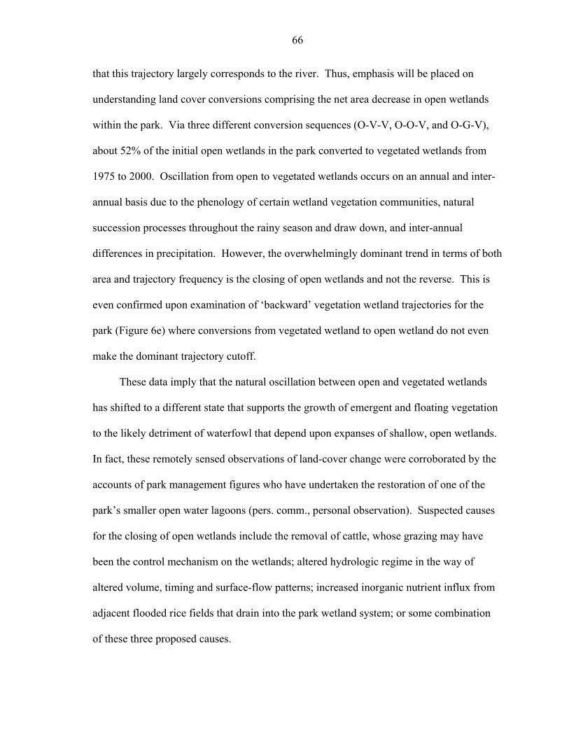
66

that this trajectory largely corresponds to the river. Thus, emphasis will be placed on

understanding land cover conversions comprising the net area decrease in open wetlands

within the park. Via three different conversion sequences (O-V-V, O-O-V, and O-G-V),

about 52% of the initial open wetlands in the park converted to vegetated wetlands from

1975 to 2000. Oscillation from open to vegetated wetlands occurs on an annual and inter-

annual basis due to the phenology of certain wetland vegetation communities, natural

succession processes throughout the rainy season and draw down, and inter-annual

differences in precipitation. However, the overwhelmingly dominant trend in terms of both

area and trajectory frequency is the closing of open wetlands and not the reverse. This is

even confirmed upon examination of ‘backward’ vegetation wetland trajectories for the

park (Figure 6e) where conversions from vegetated wetland to open wetland do not even

make the dominant trajectory cutoff.

These data imply that the natural oscillation between open and vegetated wetlands

has shifted to a different state that supports the growth of emergent and floating vegetation

to the likely detriment of waterfowl that depend upon expanses of shallow, open wetlands.

In fact, these remotely sensed observations of land-cover change were corroborated by the

accounts of park management figures who have undertaken the restoration of one of the

park’s smaller open water lagoons (pers. comm., personal observation). Suspected causes

for the closing of open wetlands include the removal of cattle, whose grazing may have

been the control mechanism on the wetlands; altered hydrologic regime in the way of

altered volume, timing and surface-flow patterns; increased inorganic nutrient influx from

adjacent flooded rice fields that drain into the park wetland system; or some combination

of these three proposed causes.

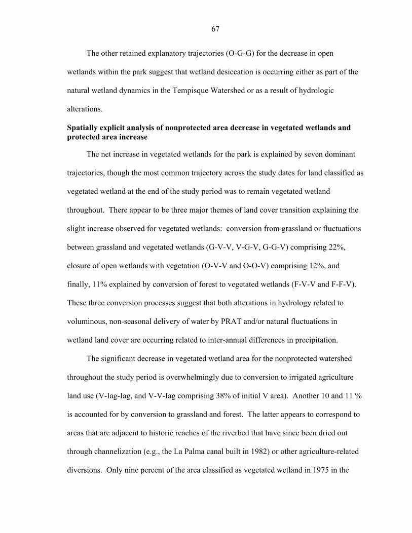
67

The other retained explanatory trajectories (O-G-G) for the decrease in open

wetlands within the park suggest that wetland desiccation is occurring either as part of the

natural wetland dynamics in the Tempisque Watershed or as a result of hydrologic

alterations.

Spatially explicit analysis of nonprotected area decrease in vegetated wetlands and protected area increase

The net increase in vegetated wetlands for the park is explained by seven dominant

trajectories, though the most common trajectory across the study dates for land classified as

vegetated wetland at the end of the study period was to remain vegetated wetland

throughout. There appear to be three major themes of land cover transition explaining the

slight increase observed for vegetated wetlands: conversion from grassland or fluctuations

between grassland and vegetated wetlands (G-V-V, V-G-V, G-G-V) comprising 22%,

closure of open wetlands with vegetation (O-V-V and O-O-V) comprising 12%, and

finally, 11% explained by conversion of forest to vegetated wetlands (F-V-V and F-F-V).

These three conversion processes suggest that both alterations in hydrology related to

voluminous, non-seasonal delivery of water by PRAT and/or natural fluctuations in

wetland land cover are occurring related to inter-annual differences in precipitation.

The significant decrease in vegetated wetland area for the nonprotected watershed

throughout the study period is overwhelmingly due to conversion to irrigated agriculture

land use (V-Iag-Iag, and V-V-Iag comprising 38% of initial V area). Another 10 and 11 %

is accounted for by conversion to grassland and forest. The latter appears to correspond to

areas that are adjacent to historic reaches of the riverbed that have since been dried out

through channelization (e.g., the La Palma canal built in 1982) or other agriculture-related

diversions. Only nine percent of the area classified as vegetated wetland in 1975 in the

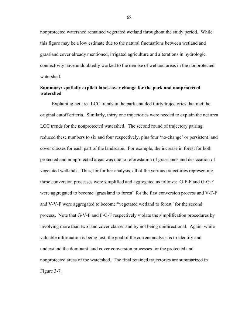
68

nonprotected watershed remained vegetated wetland throughout the study period. While

this figure may be a low estimate due to the natural fluctuations between wetland and

grassland cover already mentioned, irrigated agriculture and alterations in hydrologic

connectivity have undoubtedly worked to the demise of wetland areas in the nonprotected

watershed.

Summary: spatially explicit land-cover change for the park and nonprotected watershed

Explaining net area LCC trends in the park entailed thirty trajectories that met the

original cutoff criteria. Similarly, thirty one trajectories were needed to explain the net area

LCC trends for the nonprotected watershed. The second round of trajectory pairing

reduced these numbers to six and four respectively, plus four ‘no-change’ or persistent land

cover classes for each part of the landscape. For example, the increase in forest for both

protected and nonprotected areas was due to reforestation of grasslands and desiccation of

vegetated wetlands. Thus, for further analysis, all of the various trajectories representing

these conversion processes were simplified and aggregated as follows: G-F-F and G-G-F

were aggregated to become “grassland to forest” for the first conversion process and V-F-F

and V-V-F were aggregated to become “vegetated wetland to forest” for the second

process. Note that G-V-F and F-G-F respectively violate the simplification procedures by

involving more than two land cover classes and by not being unidirectional. Again, while

valuable information is being lost, the goal of the current analysis is to identify and

understand the dominant land cover conversion processes for the protected and

nonprotected areas of the watershed. The final retained trajectories are summarized in

Figure 3-7.

69

Principal Components Analysis (PCA): Multivariate Landscape Structure

PCA proved moderately effective in reducing the dimensionality of the data. Two

principal components with eigenvalues greater than one were extracted from the

multivariate scatter of data about the eight landscape variables to explain nearly 53% of the

total variance in the dataset (Table 3-3). Even though about half of the variance is not

accounted for by the PCA results, these two components explain more variation than would

be observed if there was no real multivariate structure to the landscape. The way in which

the landscape variables load on the two components is particularly useful at defining two

distinct dimensions of landscape variability.

The original structure matrix was used since loadings in the rotated component

matrix failed to improve or change appreciably the interpretation of the principal

components. The structure matrix (Table 3-3) reveals that the first component largely

defines the biophysical gradient of the landscape with significant loadings of elevation,

slope and distance to river. While these variables obviously covary, the correlation matrix

suggests that this loading pattern is not merely an artifact of adding redundant variables

since the bivariate correlation coefficients between pairs of the three variables range only

from 0.334 to 0.537 (Table 3-4). The positive values of all loadings except distance to

large forest illustrates that large forest patches occur mostly in the upper watershed. That

is, small distance to forest is associated with the same end of the component as high values

of elevation, slope, distance to river and distance from park boundary.

The second component largely defines the built structure of the landscape with

significant loadings of distance to roads, distance to population center, distance to the

Panamerican Highway and distance to large forest. Large distances from population

centers are associated with same the end of the component as large distances from roads

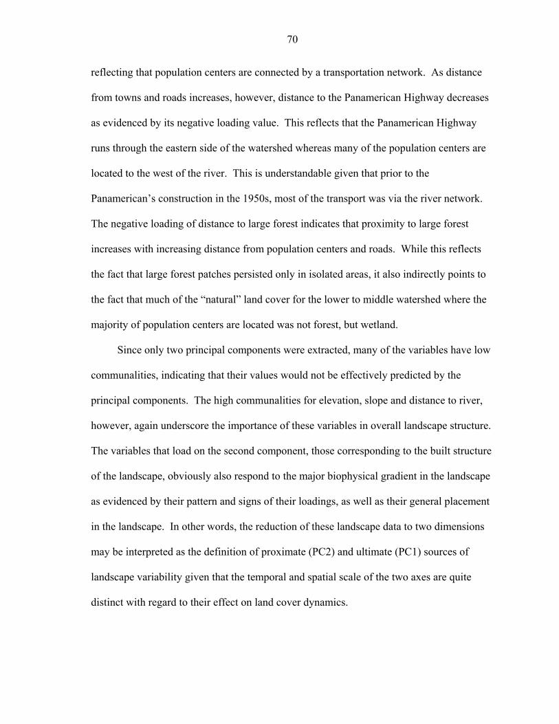
70

reflecting that population centers are connected by a transportation network. As distance

from towns and roads increases, however, distance to the Panamerican Highway decreases

as evidenced by its negative loading value. This reflects that the Panamerican Highway

runs through the eastern side of the watershed whereas many of the population centers are

located to the west of the river. This is understandable given that prior to the

Panamerican’s construction in the 1950s, most of the transport was via the river network.

The negative loading of distance to large forest indicates that proximity to large forest

increases with increasing distance from population centers and roads. While this reflects

the fact that large forest patches persisted only in isolated areas, it also indirectly points to

the fact that much of the “natural” land cover for the lower to middle watershed where the

majority of population centers are located was not forest, but wetland.

Since only two principal components were extracted, many of the variables have low

communalities, indicating that their values would not be effectively predicted by the

principal components. The high communalities for elevation, slope and distance to river,

however, again underscore the importance of these variables in overall landscape structure.

The variables that load on the second component, those corresponding to the built structure

of the landscape, obviously also respond to the major biophysical gradient in the landscape

as evidenced by their pattern and signs of their loadings, as well as their general placement

in the landscape. In other words, the reduction of these landscape data to two dimensions

may be interpreted as the definition of proximate (PC2) and ultimate (PC1) sources of

landscape variability given that the temporal and spatial scale of the two axes are quite

distinct with regard to their effect on land cover dynamics.

71

Land-Cover Change as Function of Biophysical and Social Landscape

For each net area land-cover change trend, means for biophysical and location-

relationship variables for each of the final, dominant trajectories were compared, along

with the ‘no-change’ trajectory for each land cover, for both the nonprotected (Table 3-5)

and protected (Table 3-6) parts of the landscape. Based on exploratory data analysis and

results from PCA, distance from large forest and distance from park boundary were not

included in these comparisons, as they did not generally offer any new information in

contrasting the domains of dominant, competing trajectories.

Comparing means of landscape variables for nonprotected area

For the nonprotected watershed, two explanatory trajectories were compared for the

net decrease in grassland: grassland to forest and grassland to irrigated agriculture. On

comparing the means (Table 3-5) and distributions (Figure 8) of these trajectories for all

variables measured, it is clear that these two trajectories largely occur in different

landscape domains. Grassland is converted to irrigated-agriculture land use in low, flat

areas near the river, with an average elevation of 33.73 m, average slope of 1.43% and half

the mean distance to river as the competing trajectory (4505.47 m versus 8990.44 m,

P<0.01). This trajectory is also closer to population centers and the Panamerican Highway

than the grasslands that are reforested. On average, grasslands that are reforested occur at

much higher elevations (218.04 m), steeper slopes (13.3%), farther from the river (8990.44

m), population centers and the Panamerican Highway. This comparison suggests that the

land most suitable for the current land use model (intensive agriculture) is in the lower

watershed, and grassland areas not falling within this domain are reforesting. Based on

these results, degree of isolation may also play a role in whether reforestation occurs.

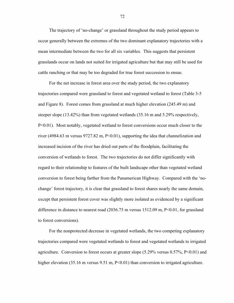
72

The trajectory of ‘no-change’ or grassland throughout the study period appears to

occur generally between the extremes of the two dominant explanatory trajectories with a

mean intermediate between the two for all six variables. This suggests that persistent

grasslands occur on lands not suited for irrigated agriculture but that may still be used for

cattle ranching or that may be too degraded for true forest succession to ensue.

For the net increase in forest area over the study period, the two explanatory

trajectories compared were grassland to forest and vegetated wetland to forest (Table 3-5

and Figure 8). Forest comes from grassland at much higher elevation (245.49 m) and

steeper slope (13.42%) than from vegetated wetlands (35.16 m and 5.29% respectively,

P<0.01). Most notably, vegetated wetland to forest conversions occur much closer to the

river (4984.63 m versus 9727.82 m, P<0.01), supporting the idea that channelization and

increased incision of the river has dried out parts of the floodplain, facilitating the

conversion of wetlands to forest. The two trajectories do not differ significantly with

regard to their relationship to features of the built landscape other than vegetated wetland

conversion to forest being farther from the Panamerican Highway. Compared with the ‘no-

change’ forest trajectory, it is clear that grassland to forest shares nearly the same domain,

except that persistent forest cover was slightly more isolated as evidenced by a significant

difference in distance to nearest road (2036.75 m versus 1512.09 m, P<0.01, for grassland

to forest conversions).

For the nonprotected decrease in vegetated wetlands, the two competing explanatory

trajectories compared were vegetated wetlands to forest and vegetated wetlands to irrigated

agriculture. Conversion to forest occurs at greater slope (5.29% versus 0.57%, P<0.01) and

higher elevation (35.16 m versus 9.51 m, P<0.01) than conversion to irrigated agriculture.

73

Since the elevation and slope are considerably greater for vegetated wetlands converting to

forest than those converting to irrigated agriculture or remaining wetlands throughout, this

suggests that the wetlands following this trajectory are likely riparian areas that have dried

out due to hydrologic alterations. However, vegetated wetlands to forest has the highest

distance from river which contradicts this idea, unless total diversion of stream flow has

occurred (i.e., stream removal). The persistent vegetated wetland trajectory has a distinct

domain in the landscape compared with the two dominant change trajectories for vegetated

wetlands. Means for all six landscape variables except distance to Panamerican Highway

were significantly different (P<0.01). Nonprotected wetlands that persisted throughout the

study period were the most isolated and occurred in the lowest, flattest parts of the

watershed.

The increase in irrigated agriculture for the nonprotected landscape is explained by

two dominant trajectories, vegetated wetlands to irrigated agriculture and grassland to

irrigated agriculture, that have been examined already in the context of explaining net

decreases in grassland and vegetated wetlands. The persistent irrigated agriculture land use

trajectory suggests that the first land to be converted was closest to the river (2418.38 m

versus 3187.7 m and 4153.19 m respectively for the other trajectories, P<0.01), which is

expected since the lone water source at the beginning of the study period was the river

itself. Grasslands converted to irrigated agriculture, as expected, have a higher (P<0.01)

mean elevation and slope (30.265 m and 1.21% ) than conversions from vegetated wetlands

(12.9 m and 0.57%). The mean distance to road for conversion from vegetated wetlands

(2338.68 m) was higher (P<0.01) than for conversions from grassland (1203.67 m)

74

indicating the high level of investment in the way of infrastructure required to implement

this land use system in much of the lower watershed.

In comparing the dominant explanatory trajectories across all net-area trends for

land-cover change in the nonprotected portion of the watershed (Table 3-5), elevation and

slope appear to be the most effective variables in defining the path of conversion for a

given starting land-cover type. Not only were all pair-wise comparisons amongst

competing trajectories found to be significantly different, the magnitudes of the differences

in means are environmentally significant as well. Boxplots of the mean elevation for each

trajectory clearly illustrate the differences in ranges (Figure 8).

Comparing means of landscape variables for protected area

The two dominant trajectories competing with the park to explain the net area

decrease in grassland area were grassland reforestation and grassland to vegetated wetland

transitions. Analogous to its landscape setting in the nonprotected area, grassland

reforestation occurs in the uplands of the park with a higher (P<0.01) mean elevation

(32.17 m) and slope (13.44%) than the grassland to wetland trajectory (8.99 m and 1.40%

respectively). Grassland reforestation in the park is further associated with uplands by

virtue of occurring farthest from the river (P<0.01) relative to conversions to vegetated

wetland or persistent grasslands (2927.98 m versus 1740.00 m or 2252.05 m respectively).

The park and nonprotected area seem to share the same dominant explanatory

trajectory, reforestation of grasslands, for reduction of grasslands and increase in forest

cover in upland areas. However, in lowlands of the park, there is no conversion to irrigated

agriculture. The lowland dominant trajectory for decrease in grasslands is the interplay

between grasslands and wetlands. This grassland to vegetated wetland trajectory occurs in

largely the same domain as persistent vegetated wetlands. That is, relative to reforesting

75

grasslands or persistent grasslands, these grasslands that transition to vegetated wetlands

occur in the lowest (8.99 m mean elevation), flattest (1.40% mean slope), and most isolated

areas of the park (P<0.01). This suggests that the park is effective in preventing direct

conversion of natural cover to direct human land use. However, since the classification

method employed was reasonably effective in offsetting land cover differences due to inter-

annual climate change, these data suggest that the park may be incurring land-cover

changes due to alterations in hydrologic regime or climatic events such as ENSO. Though

these findings are intuitive and expected, parks are still largely being managed as islands,

particularly with regard to any concept of connectivity to broader landscape processes

beyond that of habitat connectivity via corridors and reserve networks (e.g., Sanchez-

Azofeifa et al. 2003).

Again, just as in the nonprotected area, the dominant explanatory trajectories for the

increase in forest within the park are grassland to forest and vegetated wetland to forest.

The latter occurs at a lower (P<0.01) mean elevation (15.54 m) and slope (5.94%) than

grassland reforestation (32.17 m and 13.44% respectively). This corresponds to the

relationship between these two trajectories in the nonprotected landscape; however, unlike

the nonprotected area, distance to river for the two trajectories is the same (P>0.05). This

may be more of a reflection of the fact that the park is a smaller, defined area where

distance from river cannot vary significantly by virtue of its proximity to river. As in the

nonprotected watershed, persistent forest has the same relationship to reforested grasslands

in that it occurs in largely the same relative landscape domain.

Three dominant trajectories explain the increase in vegetated wetlands within the

park: the closing of open water wetlands with vegetation, transition from forest to

76

vegetated wetlands, and transition from grassland to vegetated wetlands. These

trajectories, along with persistent vegetated wetlands throughout the study period, all occur

within the same biophysical domain with no significant difference in elevation or slope

(P>0.05). Open to vegetated wetland occurs closer to the river than conversion to

vegetated wetland from grassland (1032.79 m versus 1653.10 m, P<0.01) and both of these

trajectories occur in areas more isolated in terms of distance to the Panamerican and

population centers (P>0.05). Otherwise, these trajectories are none-too-distinguished by

their respective means for landscape variables, suggesting that an unmeasured variable

such as hydrology may play a bigger part than the landscape variables measured here in

determining wetland dynamics within the park.

The final net area change in land cover for the park is the decrease in open wetlands

explained by both conversion to vegetated wetlands and desiccation to become grassland.

The means for these two trajectories for all landscape variables measured do not differ

significantly (P>0.05). When these two trajectories of open wetland change are compared

with persistent open wetlands in the park, results show that the three differ only with

respect to mean distance from river (P>0.05). Persistent open wetlands occur, on average,

491.37 m from the river, versus 1032.79 m and 1635.20 m for open to vegetated wetland

conversions or open wetland desiccation, respectively. As with the previous case, these

results suggest that hydrology, precipitation or other unmapped variables are more-closely

associated with the path/trajectory taken by a given open wetland pixel over the course of

the study period than the landscape domain defined by these six biophysical and location-

relationship variables.

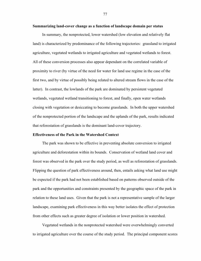
77

Summarizing land-cover change as a function of landscape domain per status

In summary, the nonprotected, lower watershed (low elevation and relatively flat

land) is characterized by predominance of the following trajectories: grassland to irrigated

agriculture, vegetated wetlands to irrigated agriculture and vegetated wetlands to forest.

All of these conversion processes also appear dependant on the correlated variable of

proximity to river (by virtue of the need for water for land use regime in the case of the

first two, and by virtue of possibly being related to altered stream flows in the case of the

latter). In contrast, the lowlands of the park are dominated by persistent vegetated

wetlands, vegetated wetland transitioning to forest, and finally, open water wetlands

closing with vegetation or desiccating to become grasslands. In both the upper watershed

of the nonprotected portion of the landscape and the uplands of the park, results indicated

that reforestation of grasslands is the dominant land-cover trajectory.

Effectiveness of the Park in the Watershed Context

The park was shown to be effective in preventing absolute conversion to irrigated

agriculture and deforestation within its bounds. Conservation of wetland land cover and

forest was observed in the park over the study period, as well as reforestation of grasslands.

Flipping the question of park effectiveness around, then, entails asking what land use might

be expected if the park had not been established based on patterns observed outside of the

park and the opportunities and constraints presented by the geographic space of the park in

relation to these land uses. Given that the park is not a representative sample of the larger

landscape, examining park effectiveness in this way better isolates the effect of protection

from other effects such as greater degree of isolation or lower position in watershed.

Vegetated wetlands in the nonprotected watershed were overwhelmingly converted

to irrigated agriculture over the course of the study period. The principal component scores

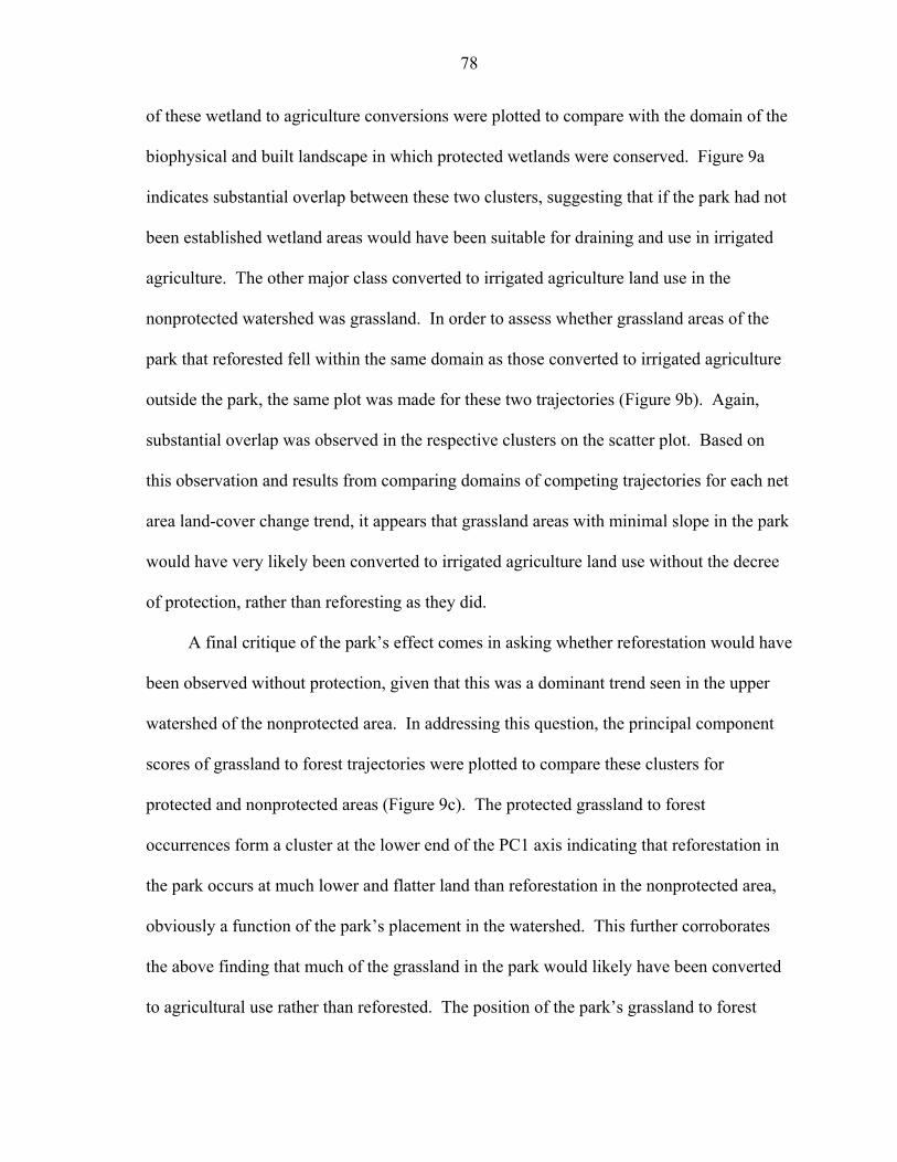
78

of these wetland to agriculture conversions were plotted to compare with the domain of the

biophysical and built landscape in which protected wetlands were conserved. Figure 9a

indicates substantial overlap between these two clusters, suggesting that if the park had not

been established wetland areas would have been suitable for draining and use in irrigated

agriculture. The other major class converted to irrigated agriculture land use in the

nonprotected watershed was grassland. In order to assess whether grassland areas of the

park that reforested fell within the same domain as those converted to irrigated agriculture

outside the park, the same plot was made for these two trajectories (Figure 9b). Again,

substantial overlap was observed in the respective clusters on the scatter plot. Based on

this observation and results from comparing domains of competing trajectories for each net

area land-cover change trend, it appears that grassland areas with minimal slope in the park

would have very likely been converted to irrigated agriculture land use without the decree

of protection, rather than reforesting as they did.

A final critique of the park’s effect comes in asking whether reforestation would have

been observed without protection, given that this was a dominant trend seen in the upper

watershed of the nonprotected area. In addressing this question, the principal component

scores of grassland to forest trajectories were plotted to compare these clusters for

protected and nonprotected areas (Figure 9c). The protected grassland to forest

occurrences form a cluster at the lower end of the PC1 axis indicating that reforestation in

the park occurs at much lower and flatter land than reforestation in the nonprotected area,

obviously a function of the park’s placement in the watershed. This further corroborates

the above finding that much of the grassland in the park would likely have been converted

to agricultural use rather than reforested. The position of the park’s grassland to forest

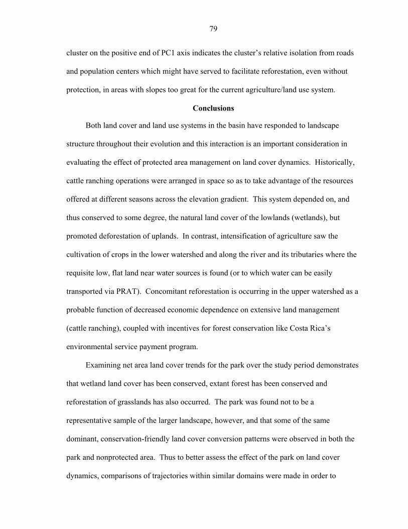
79

cluster on the positive end of PC1 axis indicates the cluster’s relative isolation from roads

and population centers which might have served to facilitate reforestation, even without

protection, in areas with slopes too great for the current agriculture/land use system.

Conclusions

Both land cover and land use systems in the basin have responded to landscape

structure throughout their evolution and this interaction is an important consideration in

evaluating the effect of protected area management on land cover dynamics. Historically,

cattle ranching operations were arranged in space so as to take advantage of the resources

offered at different seasons across the elevation gradient. This system depended on, and

thus conserved to some degree, the natural land cover of the lowlands (wetlands), but

promoted deforestation of uplands. In contrast, intensification of agriculture saw the

cultivation of crops in the lower watershed and along the river and its tributaries where the

requisite low, flat land near water sources is found (or to which water can be easily

transported via PRAT). Concomitant reforestation is occurring in the upper watershed as a

probable function of decreased economic dependence on extensive land management

(cattle ranching), coupled with incentives for forest conservation like Costa Rica’s

environmental service payment program.

Examining net area land cover trends for the park over the study period demonstrates

that wetland land cover has been conserved, extant forest has been conserved and

reforestation of grasslands has also occurred. The park was found not to be a

representative sample of the larger landscape, however, and that some of the same

dominant, conservation-friendly land cover conversion patterns were observed in both the

park and nonprotected area. Thus to better assess the effect of the park on land cover

dynamics, comparisons of trajectories within similar domains were made in order to

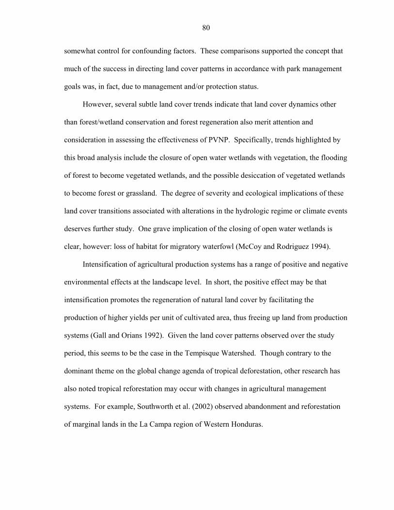
80

somewhat control for confounding factors. These comparisons supported the concept that

much of the success in directing land cover patterns in accordance with park management

goals was, in fact, due to management and/or protection status.

However, several subtle land cover trends indicate that land cover dynamics other

than forest/wetland conservation and forest regeneration also merit attention and

consideration in assessing the effectiveness of PVNP. Specifically, trends highlighted by

this broad analysis include the closure of open water wetlands with vegetation, the flooding

of forest to become vegetated wetlands, and the possible desiccation of vegetated wetlands

to become forest or grassland. The degree of severity and ecological implications of these

land cover transitions associated with alterations in the hydrologic regime or climate events

deserves further study. One grave implication of the closing of open water wetlands is

clear, however: loss of habitat for migratory waterfowl (McCoy and Rodriguez 1994).

Intensification of agricultural production systems has a range of positive and negative

environmental effects at the landscape level. In short, the positive effect may be that

intensification promotes the regeneration of natural land cover by facilitating the

production of higher yields per unit of cultivated area, thus freeing up land from production

systems (Gall and Orians 1992). Given the land cover patterns observed over the study

period, this seems to be the case in the Tempisque Watershed. Though contrary to the

dominant theme on the global change agenda of tropical deforestation, other research has

also noted tropical reforestation may occur with changes in agricultural management

systems. For example, Southworth et al. (2002) observed abandonment and reforestation

of marginal lands in the La Campa region of Western Honduras.

81

The negative effects of intensification, however, are more widely recognized. These

include nutrient inputs from fertilizers that contaminate water courses, contributions of

gases related to climate change, soil erosion, and a suite of ecological problems related to

irrigation (Gregory et al. 2002), often the cornerstone of agricultural intensification.

Irrigation systems are known to affect the extent, quality and mosaic pattern of wetlands in

several ways. They cause the direct conversion of wetlands through drainage (Niering

1988). They may desiccate and shrink the size of wetlands through competition for water

(Lemly et al. 2000) via surface extraction, channelization (Shankman 1996) and subsurface

irrigation drainage (Lemly 1994). Amplified pollution in the way of increased fertilizer;

herbicide and pesticides affect the vegetation communities and wildlife species that depend

upon them. And finally, cumulative alterations in natural surface flow regimes affect the

spatial and temporal patterns of biological productivity and thus the potential for wetland

floodplain habitats to act as sources and sinks for organic matter (Ward and Stanford

1995). All or any combination of these effects may be occurring in the Tempisque River

Watershed with grave implications for the wetland mosaic and other habitats that Palo

Verde National Park seeks to conserve.

The park represents a large portion of the only remaining natural vegetation left in

the lowest part of the watershed. The observed changes in its wetland mosaic may have

implications not only for wildlife but possibly for forest systems far upslope from it

(Lawton et al. 2001). Clearly the park was shown to be effective in the immediate sense in

that it conserved wetlands and promoted reforestation. However, long-term conservation

of Palo Verde’s unique habitat mosaic and biodiversity must be managed within the

82

context of the entire watershed. Similarly, continuation of the services and benefits that the

upper watershed receives from the park also requires a landscape perspective.

Three major points conclude this case study of the protected area management of

Palo Verde National Park within its watershed context. First, the shortcomings of Palo

Verde National Park in conserving natural land cover appear to result from factors that are

difficult to measure and which are rarely, if ever, included on the list of factors often

considered in evaluating the effectiveness of protected areas. These include effects of

fragmented or enhanced hydrologic connectivity with the wider landscape and the ability to

absorb shocks posed by periodic climate events that may only be exacerbated with

increasing global climate change.

Secondly, the important land cover dynamics seemingly related to alterations in

hydrologic regimes in this landscape were only revealed by using a land-cover

classification scheme with higher taxonomic resolution than those normally employed in

remotely sensed land cover studies of tropical reserves. Nonetheless, this increase in

thematic resolution poses data management and interpretation challenges that were,

perhaps, not treated in the most effective possible way in this analysis, despite the attempt

to establish consistent data reduction rules. Also pointed out by this study is the limitation

of categorical land cover data in assessing ecological value of land cover alterations.

Clearly, one direction for future research within this basin may be use of continuous land

cover data (e.g., vegetation indices) to better describe and capture the nuances of land

cover transitions and qualitative changes within a single, non-converting land-cover type

(Southworth, et al. 2004).

83

Finally, case studies of protected areas and protected area networks in their

watershed contexts contribute to a more complete understanding of the ways in which

parks are affected by current and potential threats originating beyond their borders,

including hydrologic alterations (Pringle 2001). This contextual approach also facilitates

an understanding of what land cover and land uses might be expected if protection were not

in place, an approach that may also be useful for predictive modeling during planning

phase of reserve establishment or during adaptive management activities existing protected

areas.

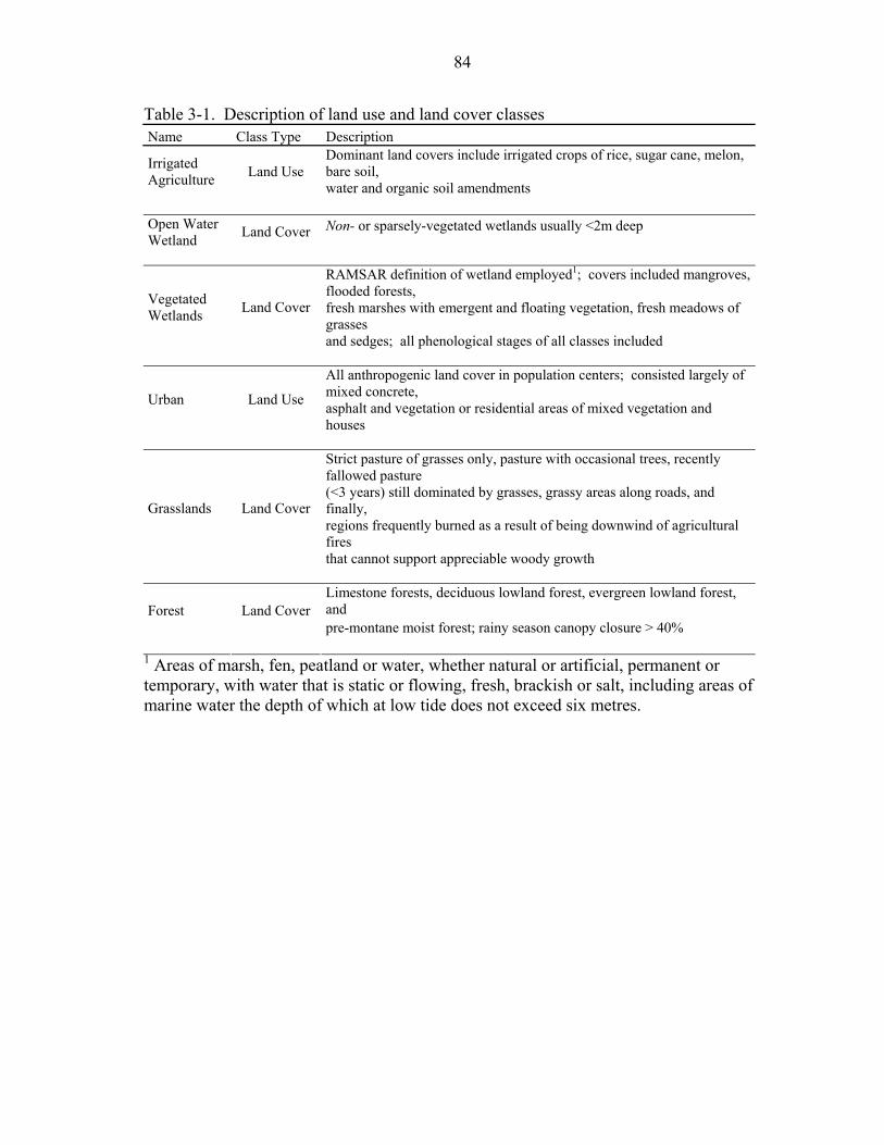
84

Table 3-1. Description of land use and land cover classes Name Class Type Description

Dominant land covers include irrigated crops of rice, sugar cane, melon, bare soil, water and organic soil amendments

Irrigated Agriculture

Land Use

Non- or sparsely-vegetated wetlands usually <2m deep Open Water

Wetland

Land Cover

RAMSAR definition of wetland employed1; covers included mangroves, flooded forests, fresh marshes with emergent and floating vegetation, fresh meadows of grasses

Vegetated Wetlands

Land Cover

and sedges; all phenological stages of all classes included All anthropogenic land cover in population centers; consisted largely of mixed concrete, Urban

Land Use

asphalt and vegetation or residential areas of mixed vegetation and houses Strict pasture of grasses only, pasture with occasional trees, recently fallowed pasture (<3 years) still dominated by grasses, grassy areas along roads, and finally, regions frequently burned as a result of being downwind of agricultural fires

Grasslands

Land Cover

that cannot support appreciable woody growth Limestone forests, deciduous lowland forest, evergreen lowland forest, and pre-montane moist forest; rainy season canopy closure > 40%

Forest

Land Cover

1 Areas of marsh, fen, peatland or water, whether natural or artificial, permanent or temporary, with water that is static or flowing, fresh, brackish or salt, including areas of marine water the depth of which at low tide does not exceed six metres.

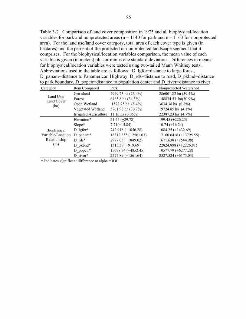
85

Table 3-2. Comparison of land cover composition in 1975 and all biophysical/location variables for park and nonprotected areas (n = 1140 for park and n = 1163 for nonprotected area). For the land use/land cover category, total area of each cover type is given (in hectares) and the percent of the protected or nonprotected landscape segment that it comprises. For the biophysical/location variables comparison, the mean value of each variable is given (in meters) plus or minus one standard deviation. Differences in means for biophysical/location variables were tested using two-tailed Mann Whitney tests. Abbreviations used in the table are as follows: D_lgfor=distance to large forest, D_panam=distance to Panamerican Highway, D_rds=distance to road, D_pkbnd=distance to park boundary, D_popctr=distance to population center and D_river=distance to river. Category Item Compared Park Nonprotected Watershed

Grassland 4949.73 ha (26.4%) 286001.82 ha (59.4%) Forest 6463.8 ha (34.5%) 148834.53 ha(30.9%) Open Wetland 1572.75 ha (8.4%) 3634.38 ha (0.8%) Vegetated Wetland 5761.98 ha (30.7%) 19724.85 ha (4.1%)

Land Use/ Land Cover

(ha)

Irrigated Agriculture 11.16 ha (0.06%) 22387.23 ha (4.7%) Elevation* 21.45 (+29.78) 199.45 (+226.25) Slope* 7.71(+15.84) 10.74 (+16.24) D_lgfor* 742.918 (+1056.28) 1084.25 (+1432.69) D_panam* 18312.355 (+2561.03) 17160.6418 (+13795.55) D_rds* 2977.03 (+1849.02) 1671.638 (+1544.98) D_pkbnd* 1315.39 (+919.69) 22824.898 (+12226.81) D_popctr* 15698.94 (+4852.45) 10577.79 (+6277.28)

Biophysical Variable/Location

Relationship (m)

D_river* 2277.89 (+1561.64) 8327.524 (+6175.03) * Indicates significant difference at alpha = 0.01

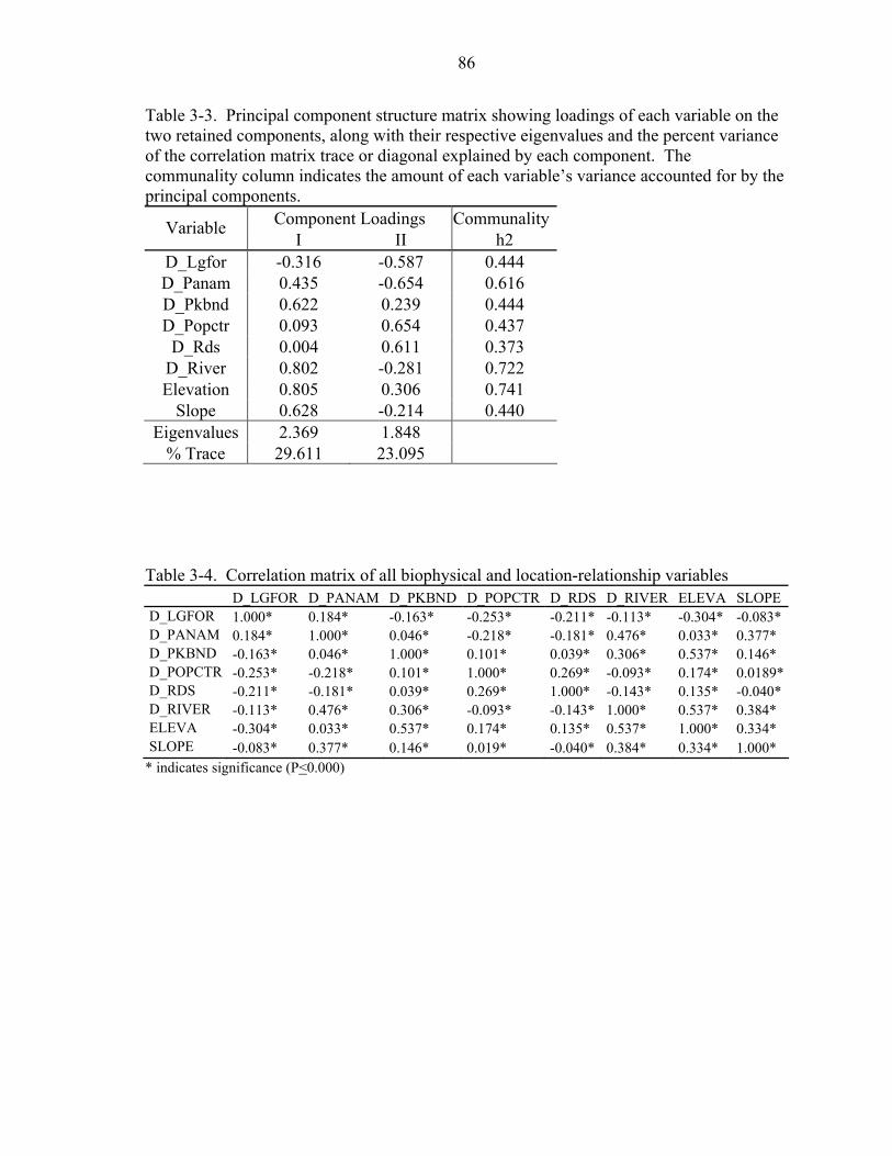
86

Table 3-3. Principal component structure matrix showing loadings of each variable on the two retained components, along with their respective eigenvalues and the percent variance of the correlation matrix trace or diagonal explained by each component. The communality column indicates the amount of each variable’s variance accounted for by the principal components.

Component Loadings CommunalityVariable I II h2

D_Lgfor -0.316 -0.587 0.444 D_Panam 0.435 -0.654 0.616 D_Pkbnd 0.622 0.239 0.444 D_Popctr 0.093 0.654 0.437

D_Rds 0.004 0.611 0.373 D_River 0.802 -0.281 0.722 Elevation 0.805 0.306 0.741

Slope 0.628 -0.214 0.440 Eigenvalues 2.369 1.848

% Trace 29.611 23.095 Table 3-4. Correlation matrix of all biophysical and location-relationship variables D_LGFOR D_PANAM D_PKBND D_POPCTR D_RDS D_RIVER ELEVA SLOPE D_LGFOR 1.000* 0.184* -0.163* -0.253* -0.211* -0.113* -0.304* -0.083* D_PANAM 0.184* 1.000* 0.046* -0.218* -0.181* 0.476* 0.033* 0.377* D_PKBND -0.163* 0.046* 1.000* 0.101* 0.039* 0.306* 0.537* 0.146* D_POPCTR -0.253* -0.218* 0.101* 1.000* 0.269* -0.093* 0.174* 0.0189*D_RDS -0.211* -0.181* 0.039* 0.269* 1.000* -0.143* 0.135* -0.040* D_RIVER -0.113* 0.476* 0.306* -0.093* -0.143* 1.000* 0.537* 0.384* ELEVA -0.304* 0.033* 0.537* 0.174* 0.135* 0.537* 1.000* 0.334* SLOPE -0.083* 0.377* 0.146* 0.019* -0.040* 0.384* 0.334* 1.000*

* indicates significance (P<0.000)

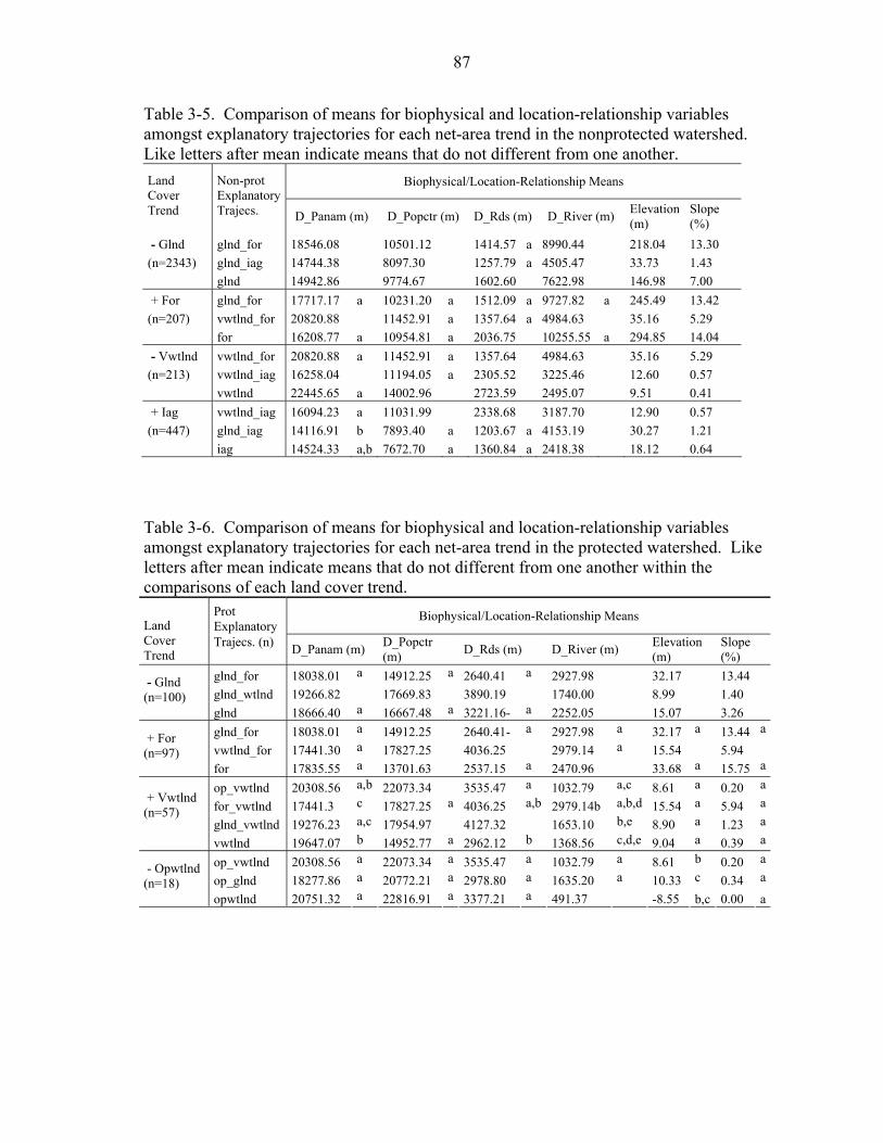
87

Table 3-5. Comparison of means for biophysical and location-relationship variables amongst explanatory trajectories for each net-area trend in the nonprotected watershed. Like letters after mean indicate means that do not different from one another.

Biophysical/Location-Relationship Means Land Cover Trend

Non-prot Explanatory Trajecs.

D_Panam (m) D_Popctr (m) D_Rds (m) D_River (m) Elevation (m)

Slope (%)

- Glnd glnd_for 18546.08 10501.12 1414.57 a 8990.44 218.04 13.30 (n=2343) glnd_iag 14744.38 8097.30 1257.79 a 4505.47 33.73 1.43 glnd 14942.86 9774.67 1602.60 7622.98 146.98 7.00 + For glnd_for 17717.17 a 10231.20 a 1512.09 a 9727.82 a 245.49 13.42 (n=207) vwtlnd_for 20820.88 11452.91 a 1357.64 a 4984.63 35.16 5.29 for 16208.77 a 10954.81 a 2036.75 10255.55 a 294.85 14.04 - Vwtlnd vwtlnd_for 20820.88 a 11452.91 a 1357.64 4984.63 35.16 5.29 (n=213) vwtlnd_iag 16258.04 11194.05 a 2305.52 3225.46 12.60 0.57 vwtlnd 22445.65 a 14002.96 2723.59 2495.07 9.51 0.41 + Iag vwtlnd_iag 16094.23 a 11031.99 2338.68 3187.70 12.90 0.57 (n=447) glnd_iag 14116.91 b 7893.40 a 1203.67 a 4153.19 30.27 1.21 iag 14524.33 a,b 7672.70 a 1360.84 a 2418.38 18.12 0.64

Table 3-6. Comparison of means for biophysical and location-relationship variables amongst explanatory trajectories for each net-area trend in the protected watershed. Like letters after mean indicate means that do not different from one another within the comparisons of each land cover trend.

Prot Explanatory

Biophysical/Location-Relationship Means Land Cover Trend

Trajecs. (n) D_Panam (m) D_Popctr (m) D_Rds (m) D_River (m) Elevation

(m) Slope (%)

glnd_for 18038.01 a 14912.25 a 2640.41 a 2927.98 32.17 13.44 glnd_wtlnd 19266.82 17669.83 3890.19 1740.00 8.99 1.40

- Glnd (n=100) glnd 18666.40 a 16667.48 a 3221.16- a 2252.05 15.07 3.26

glnd_for 18038.01 a 14912.25 2640.41- a 2927.98 a 32.17 a 13.44 a

vwtlnd_for 17441.30 a 17827.25 4036.25 2979.14 a 15.54 5.94 + For (n=97) for 17835.55 a 13701.63 2537.15 a 2470.96 33.68 a 15.75 a

op_vwtlnd 20308.56 a,b 22073.34 3535.47 a 1032.79 a,c 8.61 a 0.20 a

for_vwtlnd 17441.3 c 17827.25 a 4036.25 a,b 2979.14b a,b,d 15.54 a 5.94 a

glnd_vwtlnd 19276.23 a,c 17954.97 4127.32 1653.10 b,e 8.90 a 1.23 a

+ Vwtlnd (n=57) vwtlnd 19647.07 b 14952.77 a 2962.12 b 1368.56 c,d,e 9.04 a 0.39 a

op_vwtlnd 20308.56 a 22073.34 a 3535.47 a 1032.79 a 8.61 b 0.20 a

op_glnd 18277.86 a 20772.21 a 2978.80 a 1635.20 a 10.33 c 0.34 a - Opwtlnd (n=18) opwtlnd 20751.32 a 22816.91 a 3377.21 a 491.37 -8.55 b,c 0.00 a

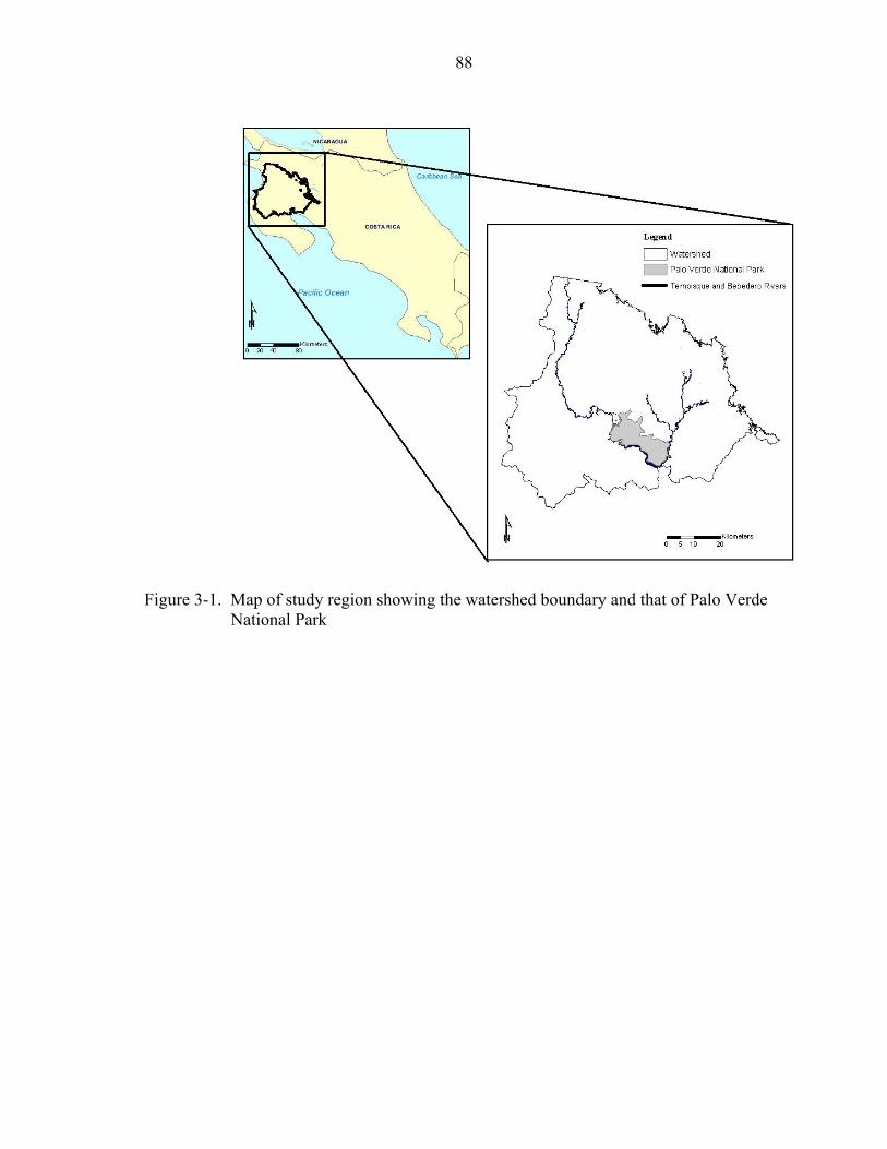
88

Figure 3-1. Map of study region showing the watershed boundary and that of Palo Verde National Park

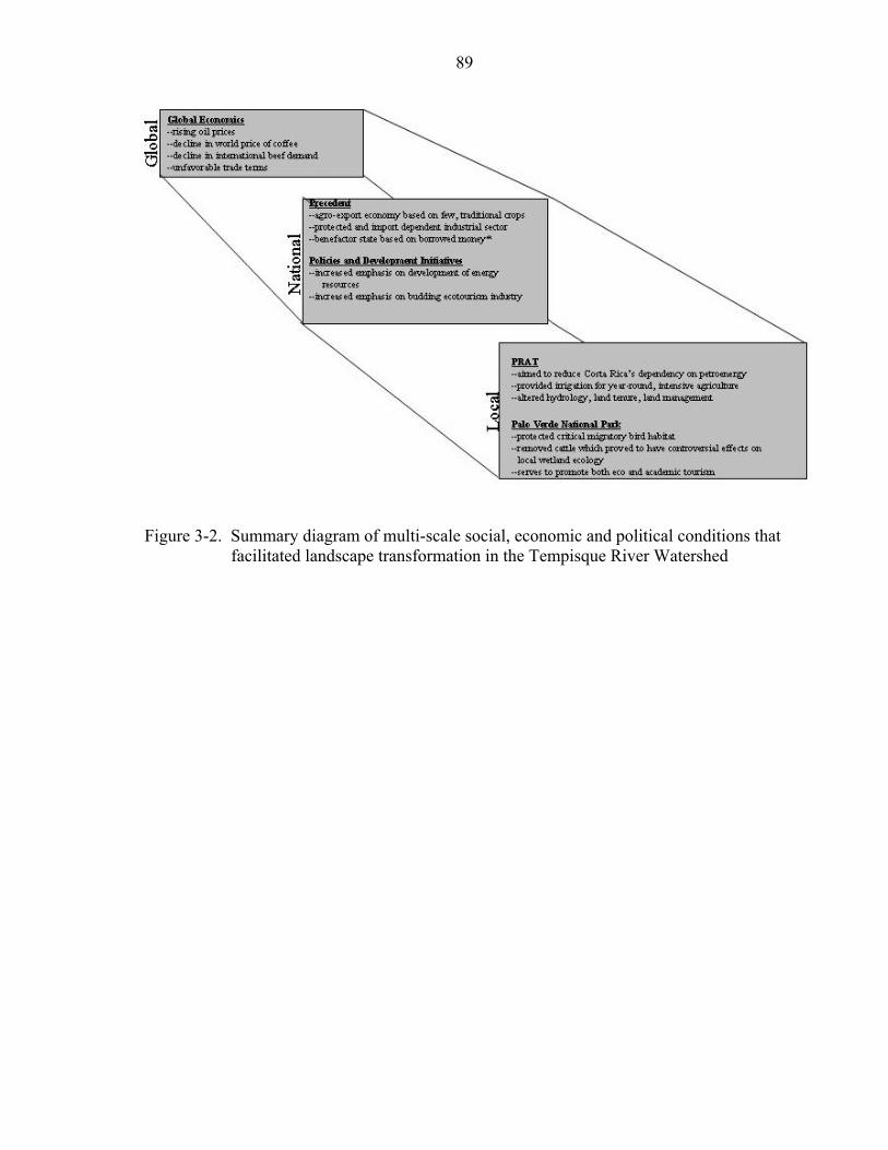
89

Figure 3-2. Summary diagram of multi-scale social, economic and political conditions that facilitated landscape transformation in the Tempisque River Watershed

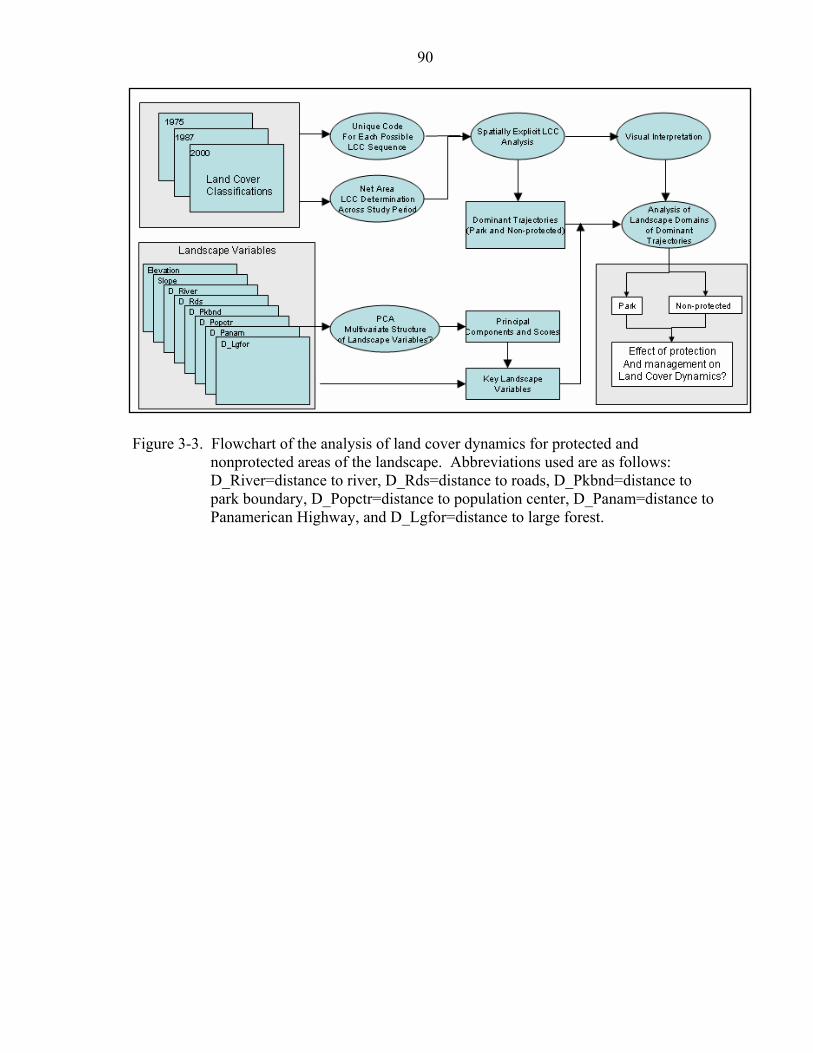
90

Figure 3-3. Flowchart of the analysis of land cover dynamics for protected and nonprotected areas of the landscape. Abbreviations used are as follows: D_River=distance to river, D_Rds=distance to roads, D_Pkbnd=distance to park boundary, D_Popctr=distance to population center, D_Panam=distance to Panamerican Highway, and D_Lgfor=distance to large forest.

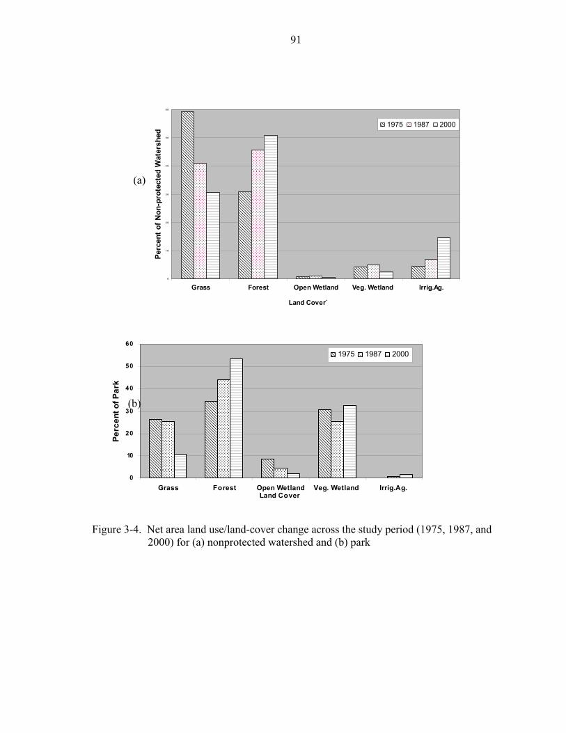
91

0

1 0

2 0

3 0

4 0

5 0

6 0

Grass Forest Open Wetland Veg. Wetland Irrig.Ag.

Land Cover`

Perc

ent o

f Non

-pro

tect

ed W

ater

shed

1975 1987 2000

(a)

0

10

20

30

40

50

60

Grass Forest Open Wetland Veg. Wetland Irrig.Ag.Land Cover

Perc

ent o

f Par

k

1975 1987 2000

(b)

Figure 3-4. Net area land use/land-cover change across the study period (1975, 1987, and 2000) for (a) nonprotected watershed and (b) park

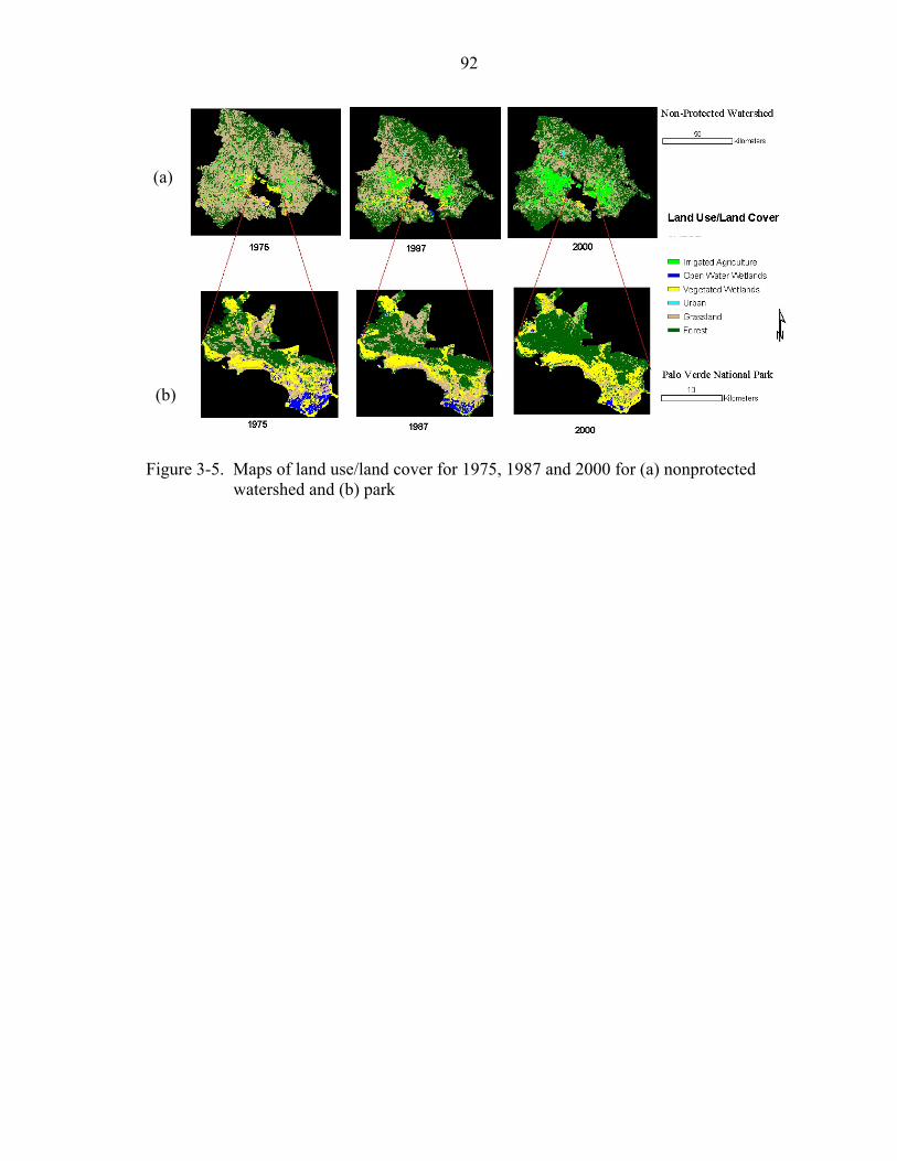
92

(a)

(b)

Figure 3-5. Maps of land use/land cover for 1975, 1987 and 2000 for (a) nonprotected watershed and (b) park

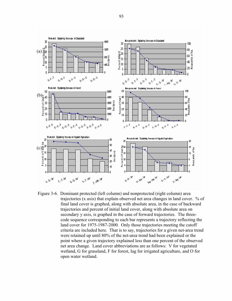
93

(a)

(b)

(c)

Figure 3-6. Dominant protected (left column) and nonprotected (right column) area trajectories (x axis) that explain observed net area changes in land cover. % of final land cover is graphed, along with absolute area, in the case of backward trajectories and percent of initial land cover, along with absolute area on secondary y axis, is graphed in the case of forward trajectories. The three-code sequence corresponding to each bar represents a trajectory reflecting the land cover for 1975-1987-2000. Only those trajectories meeting the cutoff criteria are included here. That is to say, trajectories for a given net-area trend were retained up until 80% of the net-area trend had been explained or the point where a given trajectory explained less than one percent of the observed net area change. Land cover abbreviations are as follows: V for vegetated wetland, G for grassland, F for forest, Iag for irrigated agriculture, and O for open water wetland.

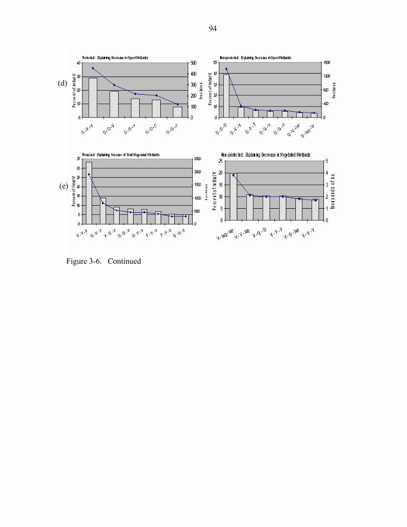
94

(d)

(e)

Figure 3-6. Continued

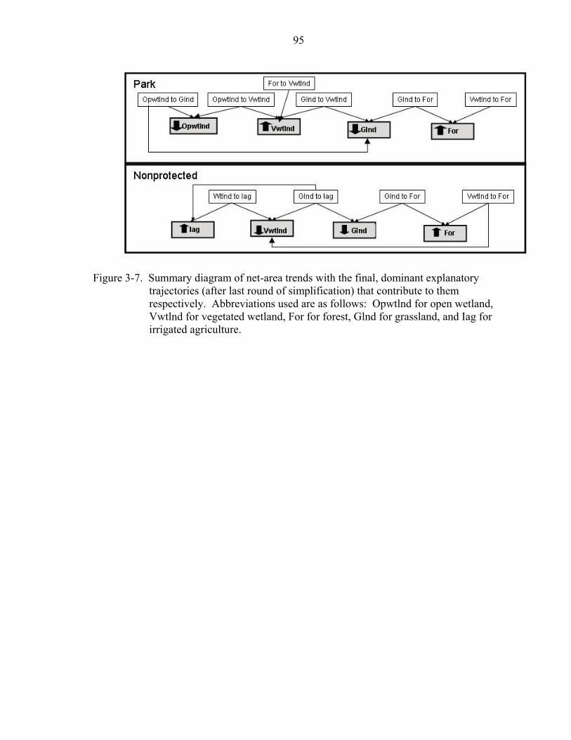
95

Figure 3-7. Summary diagram of net-area trends with the final, dominant explanatory trajectories (after last round of simplification) that contribute to them respectively. Abbreviations used are as follows: Opwtlnd for open wetland, Vwtlnd for vegetated wetland, For for forest, Glnd for grassland, and Iag for irrigated agriculture.

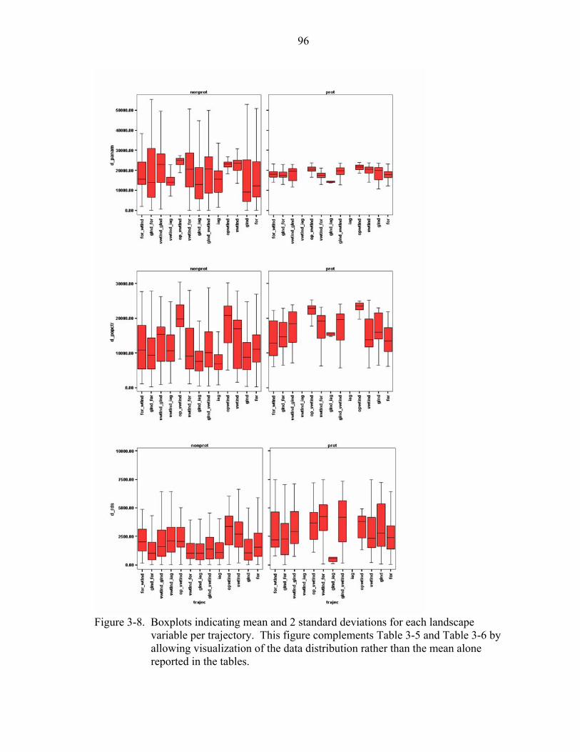
96

Figure 3-8. Boxplots indicating mean and 2 standard deviations for each landscape

variable per trajectory. This figure complements Table 3-5 and Table 3-6 by allowing visualization of the data distribution rather than the mean alone reported in the tables.

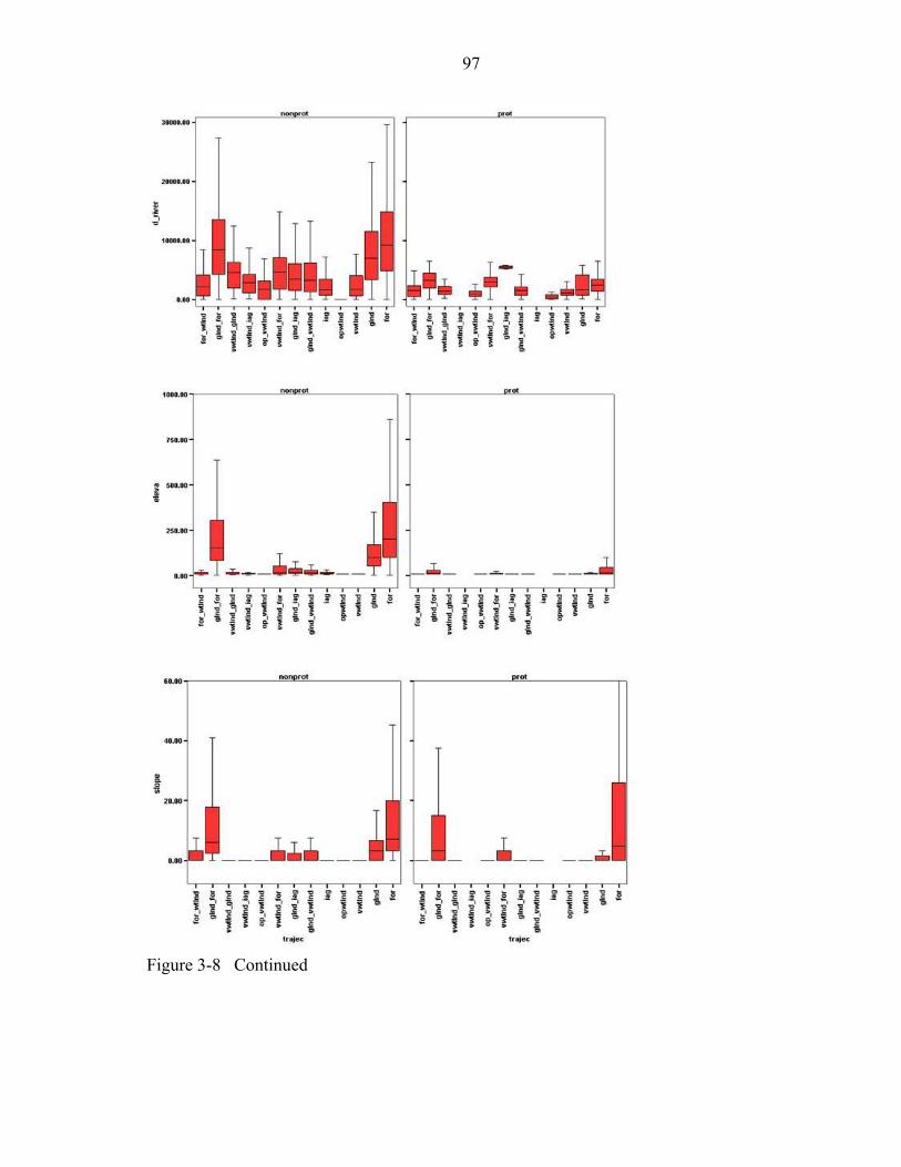
97

Figure 3-8 Continued

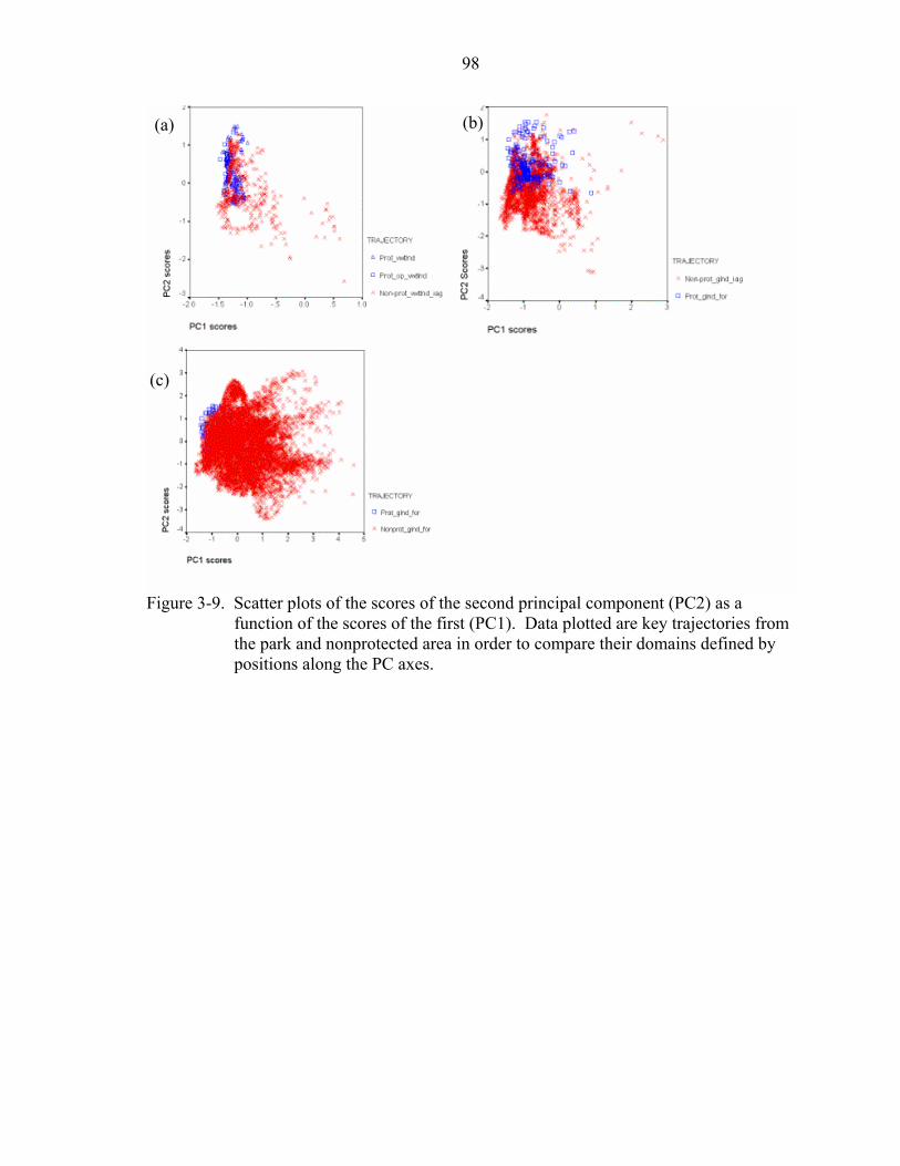
98

(b) (a)

(c)

Figure 3-9. Scatter plots of the scores of the second principal component (PC2) as a function of the scores of the first (PC1). Data plotted are key trajectories from the park and nonprotected area in order to compare their domains defined by positions along the PC axes.

CHAPTER 4 GENERAL CONCLUSIONS

One approach to gaining a more complete understanding of the effect of protected

area management on land cover is afforded by employing greater taxonomic resolution in

classification schemes and examining reserves in their larger watershed context. Given

the challenges posed by classification of land cover in landscapes with vastly different

seasonal vegetation characteristics, I needed to develop a reliable method for classifying

multiple cover types in a study region of relatively large extent. I explored an alternative

classification technique and application of land cover data derived from it in evaluating

the effect of protected area management on land cover conversion patterns.

Specifically, Chapter 2 illustrated the utility of incorporating domain knowledge in

a rule-based classification technique. Logic-oriented processing via the integration of

domain knowledge informed by ancillary data, along with the use of more than one

traditional classifier, proved effective in circumventing many of the challenges posed in

the classification of problematic tropical land cover such as deciduous tropical forest and

seasonal wetlands. Comparison of results from this technique with those of maximum

likelihood classifications on spectral data alone demonstrated a marked improvement in

classification accuracy and the elimination of systematic errors. Accuracy was improved,

without exception, for all classes in each year of the classification series relative to the

results from the traditional maximum likelihood method. Results from this case study

suggest that perhaps the greatest utility of knowledge-based processing of remotely

sensed land cover data lies in the classification of historic satellite imagery.

99

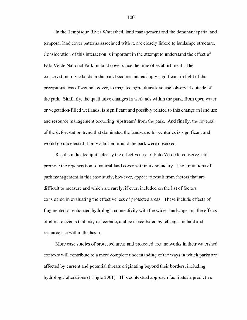
100

In the Tempisque River Watershed, land management and the dominant spatial and

temporal land cover patterns associated with it, are closely linked to landscape structure.

Consideration of this interaction is important in the attempt to understand the effect of

Palo Verde National Park on land cover since the time of establishment. The

conservation of wetlands in the park becomes increasingly significant in light of the

precipitous loss of wetland cover, to irrigated agriculture land use, observed outside of

the park. Similarly, the qualitative changes in wetlands within the park, from open water

or vegetation-filled wetlands, is significant and possibly related to this change in land use

and resource management occurring ‘upstream’ from the park. And finally, the reversal

of the deforestation trend that dominated the landscape for centuries is significant and

would go undetected if only a buffer around the park were observed.

Results indicated quite clearly the effectiveness of Palo Verde to conserve and

promote the regeneration of natural land cover within its boundary. The limitations of

park management in this case study, however, appear to result from factors that are

difficult to measure and which are rarely, if ever, included on the list of factors

considered in evaluating the effectiveness of protected areas. These include effects of

fragmented or enhanced hydrologic connectivity with the wider landscape and the effects

of climate events that may exacerbate, and be exacerbated by, changes in land and

resource use within the basin.

More case studies of protected areas and protected area networks in their watershed

contexts will contribute to a more complete understanding of the ways in which parks are

affected by current and potential threats originating beyond their borders, including

hydrologic alterations (Pringle 2001). This contextual approach facilitates a predictive

101

understanding of what land cover and land uses might be expected if protection were not

in place, an approach that may be useful both during planning phase of reserve

establishment and during adaptive management activities existing protected areas. Even

optimally functioning and connected reserves per se will only likely conserve a fraction

of the biodiversity and environmental services we seek to protect. Contextual analyses of

the effectiveness of protected area management, and the necessary techniques to perform

such evaluations, are increasingly important if parks are to be better integrated into

landscapes in which they reside.

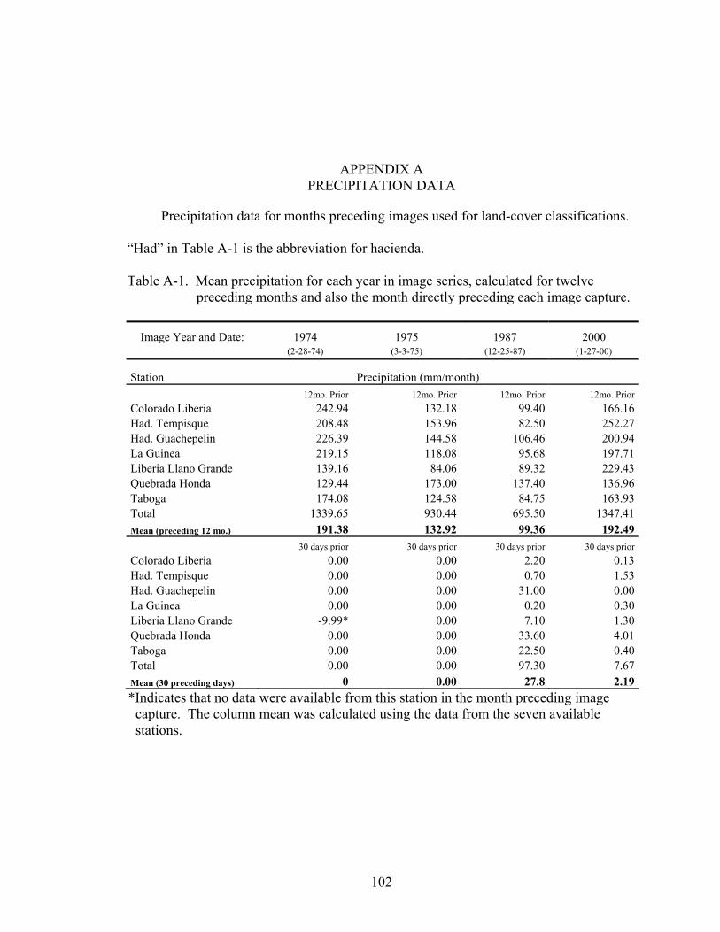
APPENDIX A PRECIPITATION DATA

Precipitation data for months preceding images used for land-cover classifications.

“Had” in Table A-1 is the abbreviation for hacienda.

Table A-1. Mean precipitation for each year in image series, calculated for twelve preceding months and also the month directly preceding each image capture.

Image Year and Date: 1974 1975 1987 2000 (2-28-74) (3-3-75) (12-25-87) (1-27-00)

Station Precipitation (mm/month)

12mo. Prior 12mo. Prior 12mo. Prior 12mo. PriorColorado Liberia 242.94 132.18 99.40 166.16Had. Tempisque 208.48 153.96 82.50 252.27Had. Guachepelin 226.39 144.58 106.46 200.94La Guinea 219.15 118.08 95.68 197.71Liberia Llano Grande 139.16 84.06 89.32 229.43Quebrada Honda 129.44 173.00 137.40 136.96Taboga 174.08 124.58 84.75 163.93Total 1339.65 930.44 695.50 1347.41Mean (preceding 12 mo.) 191.38 132.92 99.36 192.49 30 days prior 30 days prior 30 days prior 30 days priorColorado Liberia 0.00 0.00 2.20 0.13Had. Tempisque 0.00 0.00 0.70 1.53Had. Guachepelin 0.00 0.00 31.00 0.00La Guinea 0.00 0.00 0.20 0.30Liberia Llano Grande -9.99* 0.00 7.10 1.30Quebrada Honda 0.00 0.00 33.60 4.01Taboga 0.00 0.00 22.50 0.40Total 0.00 0.00 97.30 7.67Mean (30 preceding days) 0 0.00 27.8 2.19*Indicates that no data were available from this station in the month preceding image

capture. The column mean was calculated using the data from the seven available stations.

102

Figure A-1. Time series of precipitation data across entire study period averaged across

five meteorological stations (La Guinea, Rio Colorado, Had. Tempisque, Guachepelin, and Tileran). The twelve months preceding each image used in the series are highlighted in bold and the points in the series corresponding to the month preceding each image is indicated by a triangle.

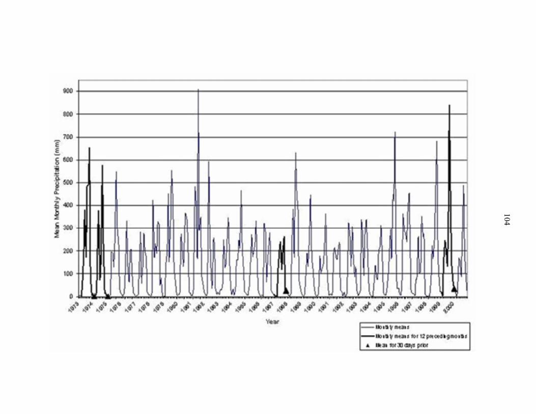
104

105

APPENDIX B LAND USE AND LAND HISTORY INTERVIEW GUIDE

Interviews conducted in Spanish and usually lasted anywhere between 20 minutes

and 3 hours.

1) Is this your property? How long have you owned or worked on this land? Did you grow up on this land or nearby here? Are there any other people around right now that might be able to help tell the history of this land?

2) Do you know where the boundaries of this parcel are? Have the boundaries always

been the same or was this parcel formerly larger/smaller? Can we take coordinates of them with GPS (present and past if their identification is possible)? Or can you show me on this topographic map approximately what the bounds of this parcel of land are and were? [If fences are present] What do these fences delineate?

3) Does your land provide you with income? If so, what do you do with your land to

make money? Is this activity what you’ve always done? Do you have access to irrigation from the government’s PRAT2 program? If so, how long have you irrigated your land? What parts and can we visit them? Was your land leveled through the PRAT program

4) What is your land like during the wet season? During the dry season? Are there any

wetlands on or near this land? What about in the past? If there are wetlands present on this land, can we visit them? Has this wetland always been here? If not, what do you think its formation is related to? How does this wetland area differ in the wet and dry seasons? Is the wetland mostly open or is there vegetation? What kind of vegetation, floating or does it grow from the soil? Is the kind of vegetation in the wetland now the same as you can remember from the past? If it has changed (e.g., from open lagoon to vegetation-filled wetland) do you remember when this change took place?

5) Depending on answers to questions 3 & 4 questions may be directed toward gaining

as much detail as possible on annual cycle of cultivation, cattle grazing practices, tree plantation management, etc.

2 Spanish acronym forProyecto Riego Arenal-Tempisque or The Arenal-Tempisque Irrigation Project.

APPENDIX C AGRICULTURAL CALENDARS

Agricultural calendars were constructed to aid in the process of interpreting satellite

imagery and aerial photographs. In addition to 29 semi-structured interviews, sources include

the Ministry of Agriculture and Livestock, Rodolfo Vega (manager Finca #4 at CATSA), Water

Management Meeting hosted by the Organization for Tropical Studies (Sept. 2002), and McCoy

(1991).

106

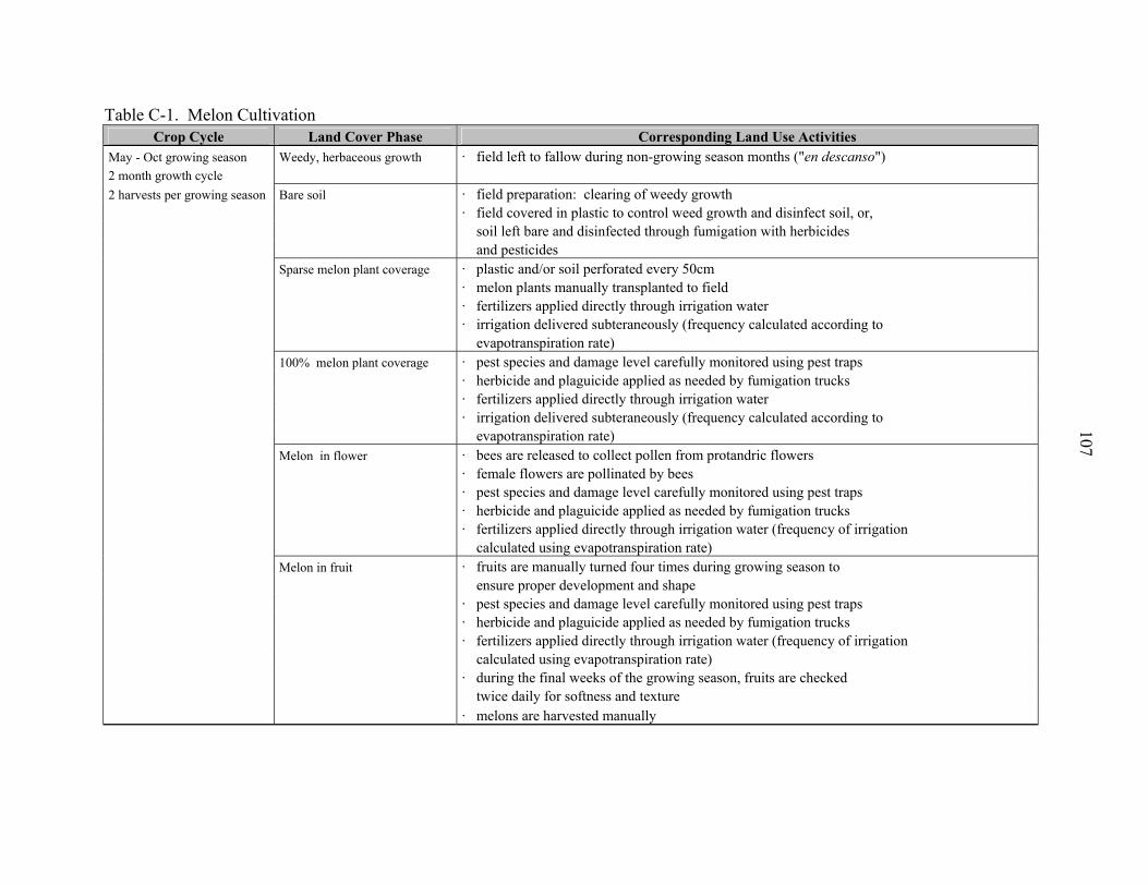
107

Table C-1. Melon Cultivation Crop Cycle Land Cover Phase Corresponding Land Use Activities

May - Oct growing season Weedy, herbaceous growth · field left to fallow during non-growing season months ("en descanso") 2 month growth cycle 2 harvests per growing season Bare soil · field preparation: clearing of weedy growth · field covered in plastic to control weed growth and disinfect soil, or, soil left bare and disinfected through fumigation with herbicides and pesticides Sparse melon plant coverage · plastic and/or soil perforated every 50cm · melon plants manually transplanted to field · fertilizers applied directly through irrigation water · irrigation delivered subteraneously (frequency calculated according to evapotranspiration rate) 100% melon plant coverage · pest species and damage level carefully monitored using pest traps · herbicide and plaguicide applied as needed by fumigation trucks · fertilizers applied directly through irrigation water · irrigation delivered subteraneously (frequency calculated according to evapotranspiration rate) Melon in flower · bees are released to collect pollen from protandric flowers · female flowers are pollinated by bees · pest species and damage level carefully monitored using pest traps · herbicide and plaguicide applied as needed by fumigation trucks · fertilizers applied directly through irrigation water (frequency of irrigation calculated using evapotranspiration rate) Melon in fruit · fruits are manually turned four times during growing season to ensure proper development and shape · pest species and damage level carefully monitored using pest traps · herbicide and plaguicide applied as needed by fumigation trucks · fertilizers applied directly through irrigation water (frequency of irrigation calculated using evapotranspiration rate) · during the final weeks of the growing season, fruits are checked twice daily for softness and texture · melons are harvested manually

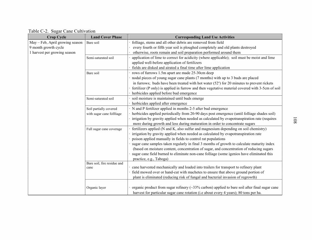
Table C-2. Sugar Cane Cultivation Crop Cycle Land Cover Phase Corresponding Land Use Activities

May – Feb, April growing season Bare soil · folliage, stems and all other debris are removed from field 9 month growth cycle · every fourth or fifth year soil is ploughed completely and old plants destroyed 1 harvest per growing season · otherwise, roots remain and soil preparation performed around them Semi-saturated soil · application of lime to correct for acidicity (where applicable); soil must be moist and lime applied well-before application of fertilizers · fields are disked and airated a final time after lime application Bare soil · rows of furrows 1.5m apart are made 25-30cm deep · nodal pieces of young sugar cane plants (7 months) with up to 3 buds are placed in furrows; buds have been treated with hot water (52o) for 20 minutes to prevent rickets · fertilizer (P only) is applied in furrow and then vegetative material covered with 3-5cm of soil · herbicides applied before bud emergence Semi-saturated soil · soil moisture is maintained until buds emerge · herbicides applied after emergence Soil partially covered · N and P fertilizer applied in months 2-5 after bud emergence with sugar cane follliage · herbicides applied periodically from 20-90 days post emergence (until folliage shades soil) · irrigation by gravity applied when needed as calculated by evapotranspiration rate (requires more during growth and less during maturation in order to concentrate sugars Full sugar cane coverage · fertilizers applied (N and K, also sulfur and magnesium depending on soil chemistry) · irrigation by gravity applied when needed as calculated by evapotranspiration rate · poison applied manually in fields to control rat populations · sugar cane samples taken regularly in final 3 months of growth to calculate maturity index (based on moisture content, concentration of sugar, and concentration of reducing sugars · sugar cane field burned to eliminate non-cane folliage (some igenios have eliminated this practice, e.g., Taboga)

Bare soil, fire residue and cane · cane harvested mechanically and loaded into trailers for transport to refinery plant

· field mowed over or hand-cut with machetes to ensure that above ground portion of plant is eliminated (reducing risk of fungal and bacterial invasion of regrowth) Organic layer · organic product from sugar refinery (~33% carbon) applied to bare soil after final sugar cane harvest for particular sugar cane rotation (i.e about every 4 years); 80 tons per ha.

108

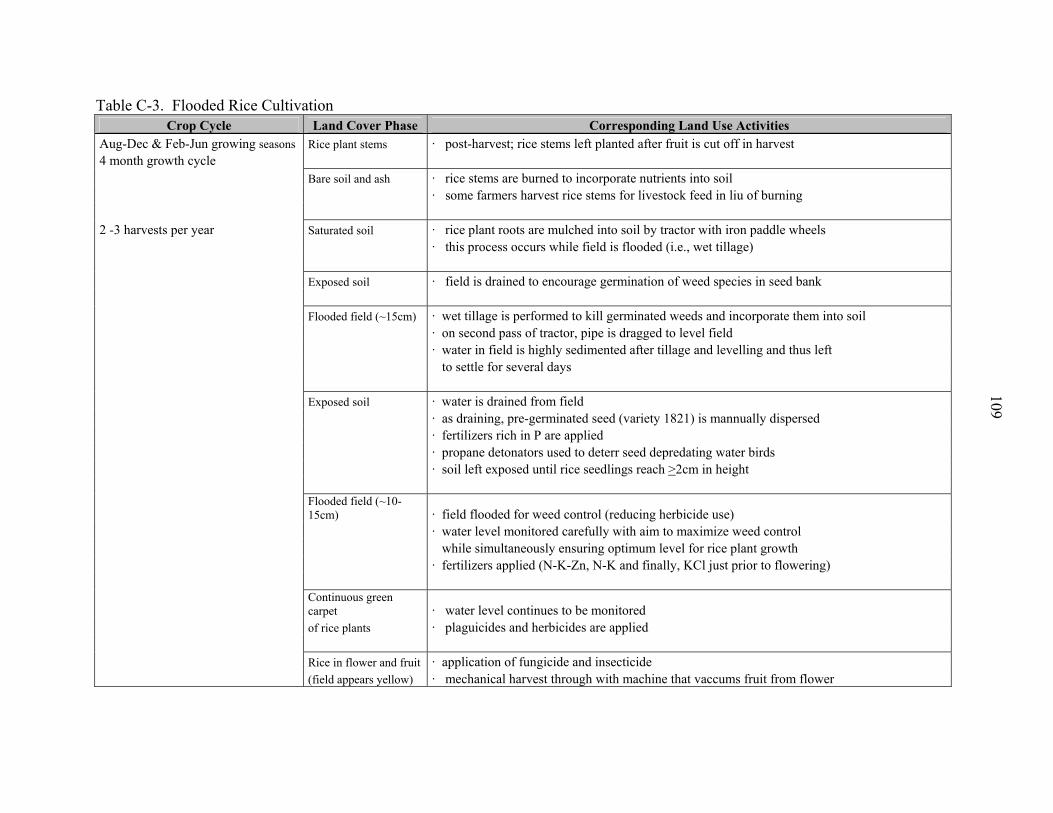
Table C-3. Flooded Rice Cultivation Crop Cycle Land Cover Phase Corresponding Land Use Activities

Aug-Dec & Feb-Jun growing seasons Rice plant stems · post-harvest; rice stems left planted after fruit is cut off in harvest 4 month growth cycle Bare soil and ash · rice stems are burned to incorporate nutrients into soil · some farmers harvest rice stems for livestock feed in liu of burning 2 -3 harvests per year Saturated soil · rice plant roots are mulched into soil by tractor with iron paddle wheels · this process occurs while field is flooded (i.e., wet tillage) Exposed soil · field is drained to encourage germination of weed species in seed bank Flooded field (~15cm) · wet tillage is performed to kill germinated weeds and incorporate them into soil · on second pass of tractor, pipe is dragged to level field · water in field is highly sedimented after tillage and levelling and thus left to settle for several days Exposed soil · water is drained from field · as draining, pre-germinated seed (variety 1821) is mannually dispersed · fertilizers rich in P are applied · propane detonators used to deterr seed depredating water birds · soil left exposed until rice seedlings reach >2cm in height

Flooded field (~10-15cm) · field flooded for weed control (reducing herbicide use)

· water level monitored carefully with aim to maximize weed control while simultaneously ensuring optimum level for rice plant growth · fertilizers applied (N-K-Zn, N-K and finally, KCl just prior to flowering)

Continuous green carpet · water level continues to be monitored

of rice plants · plaguicides and herbicides are applied Rice in flower and fruit · application of fungicide and insecticide (field appears yellow) · mechanical harvest through with machine that vaccums fruit from flower

109

APPENDIX D CHARACTERIZATIONS OF VEGETATION COMMUNITIES

Table D-1. Major wetland types and description of vegetation communities Vegetation Community Common Name Common Name Site Characteristics Watershed Context Dominant Species (English) (Spanish) Mangroves Avicennia germinans Palo de sal Saturated soils where inundation Occuring along rivers from bank up to Bravaisia integerrima Mangle pinuela is associated with tidal movements 8m into floodplain in lower watershed Conocarpus erectus Button Mangrove Mangle bontoncillo within the Nicoya Gulf along river. At Also at the Tempisque delta where the Laguncularia racemosa White Mangrove Mangle mariquita the river delta, mangroves grow in river meets the Nicoya Gulf (much of this Pelliciera rizophorae Mangle de rio classic estuarine conditions. latter area falls outside watershed). Rhizophora mangle Red Mangrove Mangle colorado

Flooded Forest Acacia collinsii Cornisuelo Seasonal saturation by rainfall and Occuring in lower watershed along rivers Acacia cornigera Cornisuelo associated peak river flows. and poorly drained areas. In riparian areas Acrocomia vinifera mangrove forest grades into flooded Bactris balanoides forest as distance from river increases Capparis odoratissima Erythrina lanceolata Inga vera Cuajiniquil Pithecellobium dulce Michiguiste

110

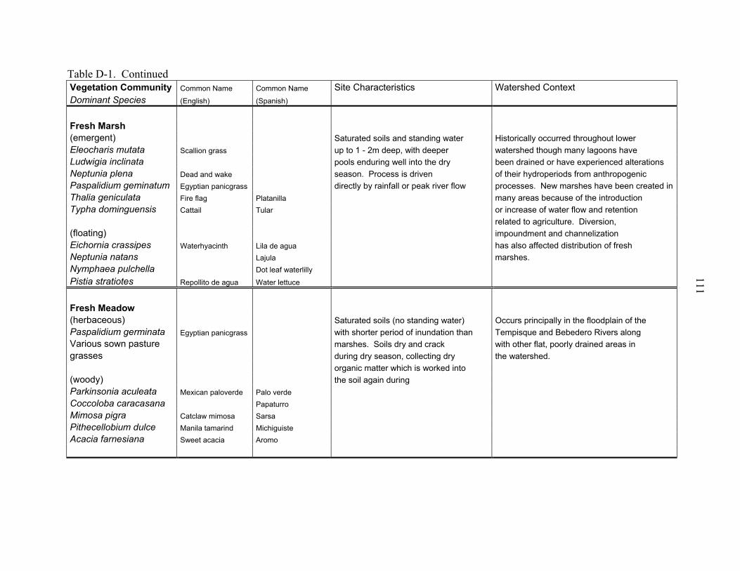
Table D-1. Continued Vegetation Community Common Name Common Name Site Characteristics Watershed Context Dominant Species (English) (Spanish) Fresh Marsh (emergent) Saturated soils and standing water Historically occurred throughout lower Eleocharis mutata Scallion grass up to 1 - 2m deep, with deeper watershed though many lagoons have Ludwigia inclinata pools enduring well into the dry been drained or have experienced alterations Neptunia plena Dead and wake season. Process is driven of their hydroperiods from anthropogenic Paspalidium geminatum Egyptian panicgrass directly by rainfall or peak river flow processes. New marshes have been created inThalia geniculata Fire flag Platanilla many areas because of the introduction Typha dominguensis Cattail Tular or increase of water flow and retention related to agriculture. Diversion, (floating) impoundment and channelization Eichornia crassipes Waterhyacinth Lila de agua has also affected distribution of fresh Neptunia natans Lajula marshes. Nymphaea pulchella Dot leaf waterlilly Pistia stratiotes Repollito de agua Water lettuce

Fresh Meadow (herbaceous) Saturated soils (no standing water) Occurs principally in the floodplain of the Paspalidium germinata Egyptian panicgrass with shorter period of inundation than Tempisque and Bebedero Rivers along Various sown pasture marshes. Soils dry and crack with other flat, poorly drained areas in grasses during dry season, collecting dry the watershed. organic matter which is worked into (woody) the soil again during Parkinsonia aculeata Mexican paloverde Palo verde Coccoloba caracasana Papaturro Mimosa pigra Catclaw mimosa Sarsa Pithecellobium dulce Manila tamarind Michiguiste Acacia farnesiana Sweet acacia Aromo

111

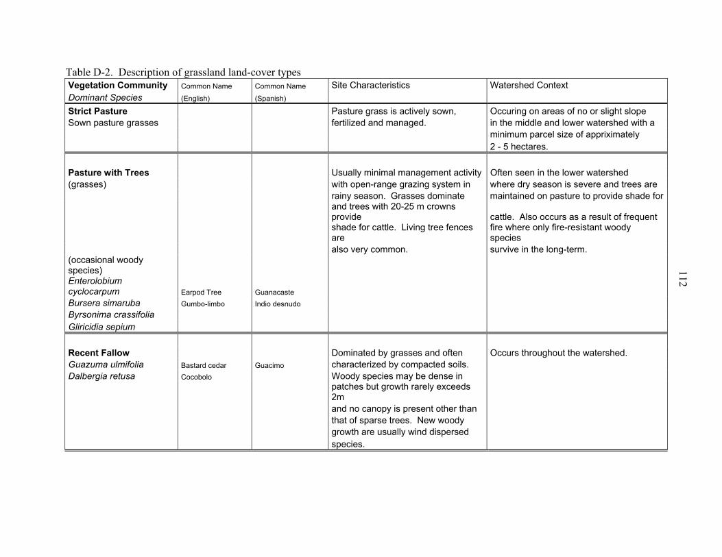
Table D-2. Description of grassland land-cover types Vegetation Community Common Name Common Name Site Characteristics Watershed Context Dominant Species (English) (Spanish) Strict Pasture Pasture grass is actively sown, Occuring on areas of no or slight slope Sown pasture grasses fertilized and managed. in the middle and lower watershed with a minimum parcel size of appriximately 2 - 5 hectares. Pasture with Trees Usually minimal management activity Often seen in the lower watershed (grasses) with open-range grazing system in where dry season is severe and trees are rainy season. Grasses dominate maintained on pasture to provide shade for

and trees with 20-25 m crowns provide cattle. Also occurs as a result of frequent

shade for cattle. Living tree fences are

fire where only fire-resistant woody species

also very common. survive in the long-term. (occasional woody species) Enterolobium cyclocarpum Earpod Tree Guanacaste Bursera simaruba Gumbo-limbo Indio desnudo Byrsonima crassifolia Gliricidia sepium Recent Fallow Dominated by grasses and often Occurs throughout the watershed. Guazuma ulmifolia Bastard cedar Guacimo characterized by compacted soils. Dalbergia retusa Cocobolo Woody species may be dense in

patches but growth rarely exceeds 2m

and no canopy is present other than that of sparse trees. New woody growth are usually wind dispersed species.

112

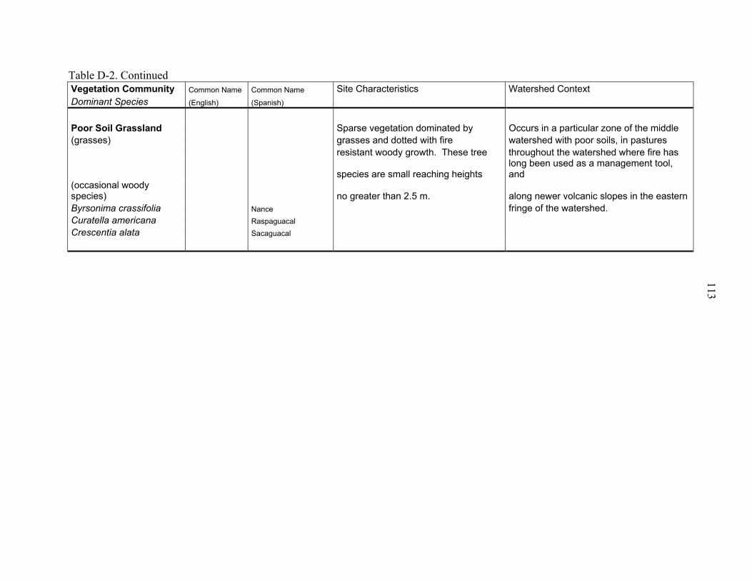
Table D-2. Continued Vegetation Community Common Name Common Name Site Characteristics Watershed Context Dominant Species (English) (Spanish) Poor Soil Grassland Sparse vegetation dominated by Occurs in a particular zone of the middle (grasses) grasses and dotted with fire watershed with poor soils, in pastures resistant woody growth. These tree throughout the watershed where fire has

species are small reaching heights long been used as a management tool, and

(occasional woody species) no greater than 2.5 m. along newer volcanic slopes in the eastern Byrsonima crassifolia Nance fringe of the watershed. Curatella americana Raspaguacal Crescentia alata Sacaguacal 113

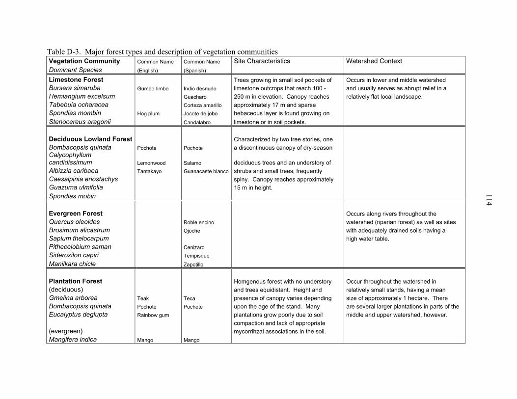
Table D-3. Major forest types and description of vegetation communities Vegetation Community Common Name Common Name Site Characteristics Watershed Context Dominant Species (English) (Spanish) Limestone Forest Trees growing in small soil pockets of Occurs in lower and middle watershed Bursera simaruba Gumbo-limbo Indio desnudo limestone outcrops that reach 100 - and usually serves as abrupt relief in a Hemiangium excelsum Guacharo 250 m in elevation. Canopy reaches relatively flat local landscape. Tabebuia ocharacea Corteza amarillo approximately 17 m and sparse Spondias mombin Hog plum Jocote de jobo hebaceous layer is found growing on Stenocereus aragonii Candalabro limestone or in soil pockets. Deciduous Lowland Forest Characterized by two tree stories, one Bombacopsis quinata Pochote Pochote a discontinuous canopy of dry-season Calycophyllum candidissimum Lemonwood Salamo deciduous trees and an understory of Albizzia caribaea Tantakayo Guanacaste blanco shrubs and small trees, frequently Caesalpinia eriostachys spiny. Canopy reaches approximately Guazuma ulmifolia 15 m in height. Spondias mobin Evergreen Forest Occurs along rivers throughout the Quercus oleoides Roble encino watershed (riparian forest) as well as sites Brosimum alicastrum Ojoche with adequately drained soils having a Sapium thelocarpum high water table. Pithecelobium saman Cenizaro Sideroxilon capiri Tempisque Manilkara chicle Zapotillo Plantation Forest Homgenous forest with no understory Occur throughout the watershed in (deciduous) and trees equidistant. Height and relatively small stands, having a mean Gmelina arborea Teak Teca presence of canopy varies depending size of approximately 1 hectare. There Bombacopsis quinata Pochote Pochote upon the age of the stand. Many are several larger plantations in parts of the Eucalyptus deglupta Rainbow gum plantations grow poorly due to soil middle and upper watershed, however. compaction and lack of appropriate (evergreen) mycorrihzal associations in the soil. Mangifera indica Mango Mango

114

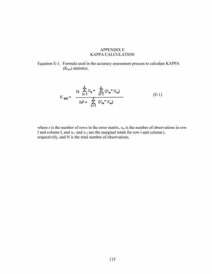
APPENDIX E KAPPA CALCULATION

Equation E-1. Formula used in the accuracy assessment process to calculate KAPPA (Khat) statistics.

(E-1)

where r is the number of rows in the error matrix, xii is the number of observations in row I and column I, and xi+ and x+i are the marginal totals for row i and column i, respectively, and N is the total number of observations.

115

LIST OF REFERENCES

ARNOLD, G.W., 1995, Incorporating landscape pattern into conservation programs. In: Hannsson, L, Fahrig, L., and G. Merriam (Eds.), Mosaic Landscapes and Ecological Processes. Chapman and Hall, London, England.

ATKINSON, P.M., and LEWIS, P., 2000, Geostatistical classification for remote sensing: an introduction. Computers and Geosciences, 26, 361-371.

AUGUSTEIJN, M.F. and WARRENDER, C.E., 1998, Wetland classification using optical and radar data and neural network classification. International Journal of Remote Sensing, 19, 8, 1545-1560.

BARBOZA, G., 1997, Rol del Ganado en la restauracion ecologica del Parque Nacional Palo Verde, Costa Rica. Apuntas del Comité Asesor Cientifico Estacion Biologica Palo Verde. Organización para Estudios Tropicales, San Jose, Costa Rica.

BERBEROGLU, S., LLOYD, C.D., ATKINSON, P.M. and CURRAN, P.J., 2000, The integration of spectral and textural information using neural networks for land cover mapping in the Mediterranean. Computers and Geosciences, 26, 385-396.

BHAGWAT, S., BROWN, N., EVANS, T., JENNINGS, S., and SAVILL, P., 2001, Parks and factors in their success. Science Aug 10, 293, 1045-1047.

BOLSTAD, P.V., and LILLESAND, T.M., 1992. Rule-based classification models: flexible integration of satellite imagery and thematic spatial data. Photogrammetric Engineering and Remote Sensing, 58, 965-971.

BRUNER, A.G., R.E. GULLISON, R.E. RICE, and G. FONSECA, 2001, Effectiveness of parks in protecting tropical biodiversity. Science, 291, 125-128.

CHAN, J.C.W., LAPORTE, N., and DeFRIES, R.S., 2003, Texture classification of logged forests in tropical Africa using machine-learning algorithms. International Journal of Remote Sensing, 24, 6, 1401-1407.

CENTRO CIENTÍFICO TROPICAL (CCT), 1998, Plan de Acción para la Cuenca del Río Tempisque. San José, Costa Rica.

116

117

CHEN, Y.Q., NIXON, M.S., and THOMAS, D.W., 1997. On texture classification. International Journal of Systems Science, 28, 7, 669-682.

CONGALTON, R.G., 1988, Using spatial autocorrelation analysis to explore the errors in maps generated from remotely sensed data. Photogrammetric Engineering and Remote Sensing, 54, 5, 587-592.

CONGALTON, R.G., 1991, A review of assessing the accuracy of classifications of remotely sensed data. Remote Sensing of Environment, 37, 35-46.

CURRAN, P.J., 2001, Remote sensing: using the spatial domain. Environmental and Ecological Statistics, 8, 331-344.

DAILY, G. C., CEBALLOS, G., PACHECO, J., SUZAN, G., and SANCHEZ-AZOFEIFA, A., 2003, Countryside biogeography of neotropical mammals: conservation opportunities in agricultural landscapes of Costa Rica. Conservation Biology, 17, 6, 1814-1826.

DANIELS, A.E., in prep., Incorporating domain knowledge and spatial relationships into land-cover classifications: a rule-based approach.

DEFRIES, R.S., HANSEN, M.C., TOWNSHEND, J.R.G., and SOHLBERG, R., 1998, Global land-cover classifications at 8km spatial resolution: the use of training data derived from Landsat imagery in decision tree classifiers. International Journal of Remote Sensing, 19, 16, 3141-3168.

DEWITT, R.P., 1977, The Inter-American Development Bank and political influence with special reference to Costa Rica. Praeger Publishers. N.Y., N.Y., USA.

FANG, J., PIAO, S., and TANG, Z., 2001, Interannual Variability in Net Primary Production and Precipitation, Science, 293, 1723.

FERNANDEZ-PRIETO, D., 2002, An iterative approach to partially supervised classifications. International Journal of Remote Sensing, 23, 18, 3887-3892.

GALL, G.A., and G.H. ORIANS, 1992, Agriculture and biological conservation. Agriculture, Ecosystems, and Environment, 42, 1-8.

GEIST, H.J., and E.F. LAMBIN, 2002, Proximate causes and underlying driving forces of tropical deforestation. BioScience, 52, 2, 143-150.

GERHARDT, K., 1993, Tree seedling development in topical dry abandoned pasture and secondary forest in Costa Rica. Journal of Vegetation Science, 4, 95-102.

118

GILL, D.E., 1988, A naturalist’s guide to the OTS Palo Verde Field Station. Organization for Tropical Studies, San Jose, Costa Rica.

GILLESPIE, T.W., A. GRIJALVA, and C.N. FARRIS., 2000, Diversity, composition and structure of tropical dry forests in Central America. Plant Ecology, 147, 37-47.

GREGORY, P.J., INGRAM, J.S.I., ANDERSSON, R., BETTS, R.A., BROVKIN, V., CHASE, T.N., GRACE, P.R., GRAY, A.J., HAMILTON, N., HARDY, T.B., HOWDEN, S.M., JENKINS, A., MEYBECK, M., OLSSON, M., ORTIZ-MONASTERIO, I.O., PALM, C., PAYNE, T., RUMMUKAINENE, M., SCULZE, R.E., THIEM, M., VALENTIN, C. and WILKINSON, M.J., 2002, Environmental consequences of alternative practices for intensifying crop production. Agriculture, Ecosystems and Environment, 88, 279-290.

HANSEN, M., DUBAYAH, R., and DeFRIES, R., 1996, Classification trees: an alternative to traditional land cover classifiers. International Journal of Remote Sensing, 17, 1075-1081.

HARCOURT, C.S., and SAYER, J. A., The conservation atlas of tropical forests: the Americas. Simon and Schuster, New York, USA.

HAYES, D.J., S.A. SADER and N.B. SCHWARTZ., 2002, Analyzing a forest conversion history database to explore the spatial and temporal characteristics of land-cover change in Guatemala’s Maya Biosphere Reserve. Landscape Ecology, 17, 299-314.

HOLDRIDGE, L.R., 1967, Life Zone Ecology. (Tropical Science Center: San Jose, Costa Rica).

HUNTER, M.L., and P. YONZON, 1993., Altitudinal distributions of birds, mammals, people, forests and parks in Nepal. Conservation Biology, 7, 420-423.

HUTCHINSON CF., 1982, Techniques for combining Landsat and ancillary data for digital classification improvement. Photogrammetric Engineering and Remote Sensing, 48, 1, 123-130.

JANSSEN, L.L.F., JAARSMA, M.N., and VANDERLINDEN, E.T.M., 1990, Integrating topographic data with remote sensing for land-cover classification. Photogrammetric Engineering and Remote Sensing, 56,11, 1503-1506.

JANZEN, D.H., 1988, Tropical dry forests: The most endangered major tropical ecosystem. Pp. 130-137. In: Wilson, E.O. (ed.), Biodiversity. National Academic Press, Washington, D.C., USA.

119

JENSEN, J.R., 2000, Introductory Digital Image Processing: A Remote Sensing Perspective (New Jersey: Prentice Hall).

JENSEN, J.R., 2000, Remote Sensing of the Environment: An Earth Resource Perspective (New Jersey: Prentice Hall).

JI, L., and PETERS, A.J., 2004, A spatial regression procedure for evaluating the relationship between AVHRR-NDVI and climate in the northern Great Plains. International Journal of Remote Sensing, 25, 2, 297-311.

JOHNSTON, R.J., 1980, Multivariate Statistical Analysis in Geography: A Primer on the General Linear Model. Longman Group Limited, New York, New York, USA.

KEPNER, W.G., WATTS, C.J., EDMONDS, C.M., MAINGI, J.K., MARSH, S.E., and LUNA, G., 2000, A landscape approach for detecting and evaluating change in a semi-arid environment. Environmental Monitoring and Assessment, 64, 179-195.

KING, R.B., 2002, Land cover mapping principles: a return to interpretation fundamentals. International Journal of Remote Sensing, 23,18, 3525-3545.

LAMBIN, E.R., 1997, Modelling and monitoring land-cover change processes in tropical regions. Progress in Physical Geography, 21,3, 375-393.

LANGFORD, M., and BELL, W., 1997a, Land cover mapping in tropical hillsides environment: a case study in the Cauca region of Colombia. International Journal of Remote Sensing, 18, 6, 1289-1306.

LANGFORD, M., and W. BELL., 1997b, Modeling and monitoring land-cover change processes in tropical regions. Progress in Physical Geography, 21, 3, 375-393.

LARA, S., BARRY, T., and SIMONSON, P, 1995, Inside Costa Rica – The essential guide to its politics, economy, society and environment. Resource Center Press. Albuquerque, New Mexico, USA.

LAWTON, R.O., U.S. NAIR, R.A. PIELKE, and R.M. WELCH., 2001, Climatic impact of tropical lowland deforestation on nearby montane cloud forests. Science, 294, 584-587.

LEMLY, A.D., 1994, Agriculture and wildlife: ecological implications of subsurface irrigation drainage. Journal of Arid Environments, 28, 85-94.

LEMLY, A.D., R.T. KINGSFORD, and J.R. THOMPSON, 2000, Irrigated agriculture and wildlife conservation: conflict on a global scale. Environmental Management, 25, 5, 485-512.

120

MARTÍNEZ-ARTAVIA, C., 2000, Papel del conflicto socio-ambiental en la gestión local/Estudio de caso de las comunidades de Bolsón y Ortega,en la Cuenca del Tempisque, Guanacaste, Costa Rica. Programa Conflicto y Colaboración en el Manejo de Recursos Naturales en América Latina (CyC), Universidad para la Paz (UPAZ), Costa Rica.

MATEO-VARGA, J., 2001, Caracteristicas generales de la cuenca del Rio Tempisque. Pages 32-72 in J.A. Jiménez and E. Gonzalez (Eds.). La Cuenca del Rio Tempisque, Perspectivas para un Manejo Integrado. Organización para Estudios Tropicales. San Jose, Costa Rica

MAXWELL, S. K., HOFFER, R. M., and CHAPMAN, P. L., 2002, AVHRR composite period selection for land-cover classification. International Journal of Remote Sensing, 23, 23, 5043-5059.

MCCOY, M.B., and J.M. RODRIGUEZ, 1994, Cattail (Typha dominguensis) eradication methods in the restoration of a tropical, seasonal, freshwater marsh. In: Mitsch, W.J. (Ed.). Global Wetlands: Old World and New. New York, New York, USA.

MCGARIGAL, K., S. CUSHMAN, and S. STAFFORD, 2000, Multivariate Statistics for Wildlife and Ecology Research. Springer-Verlag, York, PA, USA.

MERTENS, B., and E.F. LAMBIN, 2000, Land-cover change trajectories in Southern Cameroon. Annals of the American Association of Geography, 90, 3, 467-494.

MURPHY, P.G., and A.E. LUGO, 1986, Ecology of tropical dry forest. Annual Review of Ecology and Systematics, 17, 67-88.

MURAI, H., and OMATU, S., 1997, Remote sensing image analysis using a neural netowkr and knowledge-based processing, International Journal of Remote Sensing, 18, 4, 811-828.

NIERING, W.A., 1988, Endangered, threatened, and rare wetland plants and animals of the continental United States. In: Hook, D. et al. (Eds.). The Ecology and Management of Wetlands, Volume I Ecology of Wetlands. Timber Press, Portland, OR, USA.

ONSI, H.M., 2003, Designing a rule-based classifier using syntactical approach. International Journal of Remote Sensing, 24, 4, 637-647.

ORTIZ, M.J., FORMAGGIO, A.R., and EPIPHANIO, J.C., 1997, Classification of croplands through integration of remote sensing, GIS, and historical database. International Journal of Remote Sensing, 18, 1, 95-105.

121

OZESMI, S.L. and BAUER, M.E., 2002, Satellite remote sensing of wetlands. Wetlands Ecology and Management, 10, 381-402.

PARKS, S.A., and A.H. HARCOURT, 2002, Reserve size, local human density, and mammalian extinctions in U.S. protected areas. Conservation Biology, 16, 3, 800-808.

PERALTA, P. and MATHER, P., 2000, An Analysis of deforestation patterns in the extractive reserves of Acre, Amazonia from satellite imagery: a landscape ecological approach. International Journal of Remote Sensing, 21, 13/14, 2555-2570.

PETERS, G. 2001. La cuenca del Tempisque: una perspective historica. Pages 1-21 in J.A. Jiménez and E. Gonzalez (Eds.). La Cuenca del Rio Tempisque, Perspectivas para un Manejo Integrado. Organización para Estudios Tropicales. San Jose, Costa Rica.

PETIT, C., T. SCUDDER, and E. LAMBIN, 2001, Quantifying processes of land-cover change by remote sensing: resettlement and rapid land-cover changes in south-eastern Zambia. International Journal of Remote Sensing, 22, 17, 3435-3456.

PICKETT, S.T., and J. THOMPSON, 1978, Patch dynamics and the design of nature reserves. Biological Conservation, 13, 27-37.

POIANI, K.A., B.D. RICHTER, M.G. and ANDERSON, 2000, Biodiversity conservation at multiple scales: functional sites, landscapes, and networks. BioScience, 50, 2, 133-146.

PRESSEY, R.L., 1994, Ad hoc reservations: forward or backward steps in developing representative reserve systems? Conservation Biology, 8, 662-668.

PRIMACK, R., 1993, Essentials of conservation biology. Sinauer Associates, Sunderland, Massachusetts, USA.

PRINGLE, C.M., 2001, Hydrologic connectivity and the management of biological reserves: a global perspective. Ecological Applications, 11, 4, 981-998.

PRINGLE, C.M., 2003, What is hydrologic connectivity and why is it ecologically important? Hydrological Processes, 17, 2685-2689.

RAO, M., A. RABINOWITZ, and S.T. KHAING, 2002, Status review of the protected-area system in Myanmar, with recommendations for conservation planning. Conservation Biology, 16, 2, 360-368.

122

RIVARD, D.H., POITEVIN, J., PLASSE, D., CARLETON, M. and CURRIE, D.J. , 2000, Changing species richness and composition in Canadian National Parks. Conservation Biology, 14, 4, 1099-1109.

ROBERTSON, A.I., 1997, Land-water linkages in floodplain river systems: the influence of domestic stock. Pages 207-218 in N. Klomp and I. Lunt (Eds.). Frontiers in Ecology, Building the Links. Elsivier Science. Oxford, England.

RUNTE, A., 1979, National Parks: The American Experience. University of Nebraska Press, Lincoln.

SADER, S.A., AHL, D. and LIOU, W.S., 1995, Accuracy of Landsat TM and GIS rule-based methods for forest wetland classification in Maine. Remote Sensing of Environment, 53, 133-144.

SANCHEZ-AZOFEIFA, G.A., G.C. DAILY, A.PFAFF, and C. BUSCH, 2003, Integrity and isolation of Costa Rica’s national parks and biological reserves: examining the dynamics of land-cover change. Biological Conservation, 109, 123-135.

SANCHEZ-AZOFEIFA, G.A., QUESADA-MATEO, C., GONZALES- QUESADA, P. DAYANANDAN, S., and BAWA, K.S., 1999, Protected areas and conservation of biodiversity in the tropics. Conservation Biology, 13, 2, 407-411.

SANCHEZ-AZOFEIFA, G.A., B. RIVARD, J. CALVO, and I. MOORTHY, 2002, Dynamics of tropical deforestation around national parks: remote sensing of forest change on the Osa Peninsula of Costa Rica. Mountain Research and Development, 22, 4, 352-358.

SANDERSON, E.W., K.H. REDFORD, A. VEDDER, P.B. COPPOLILLO, and S.E. WARD, 2002, A conceptual model for conservation planning based on landscape species requirements. Landscape and Urban Planning, 58, 41-56.

SCHWARTZ, M.W., 1999, Choosing the appropriate scale of reserves for conservation. Annual Review of Ecological Systems, 30, 83-108.

SHANKMAN, D., 1996, Stream channelization and changing vegetation patterns in the U.S. Coastal Plain. The Geographical Review, 86, 2, 216-232.

SHARMA, K.M., and SARKAR, A., 1998, A modified contextual classification technique for remote sensing data. Photogrammetric Engineering and Remote Sensing, 64, 273-280.

SIEGEL, S., and N.J. CASTELLAN, JR., 1988, Nonparametric Statistics for the Behavioral Sciences. McGraw Hill, Singapore.

123

SIMARD, M., DEGRANDI, G., SAATCHI, S., and MAYAUX, P., 2002, Mapping tropical coastal vegetation using JERS-1 and ERS-1 radar data with a decision tree classifier. International Journal of Remote Sensing, 23, 7, 1461-1474.

SOUTHWORTH, J., 2004, An assessment of Landsat TM band 6 thermal data for analyzing land cover in tropical dry forest regions. International Journal of Remote Sensing, 25, 4, 689-706.

SOUTHWORTH, J., D. MUNROE and H. NAGENDRA, 2004, Land-cover change and fragmentation –Comparing the utility of continuous and discrete analyses for a Western Honduras region. Agriculture, Ecosystems and Environment, 101, 2-3, 185-205.

SOUTHWORTH, J., D. MUNROE, H. NAGENDRA and C. TUCKER, 2004, Forest degradation and fragmentation within Celaque National Park, Honduras. In D.G. Janelle et al. (eds.). WorldMinds: Geographical Perspectives on 100 Problems, 305-310. Kluwer Academic Publishers, Netherlands.

SOUTHWORTH, J., H. NAGENDRA, and C. TUCKER., 2002, Fragmentation of a landscape: incorporating landscape metrics into satellite analysis of land-cover change. Landscape Research, 27, 3, 253-269.

SPARKS, R.E. 1995. Need for ecosystem management of large rivers and their floodplains. BioScience, 45, 3, 168-182.

STERN, M., 2001, Parks and factors in their success. Science, 293, 1045-1047.

TERBORGH J, and VAN SCHAIK CP., 1997, Minimizing Species Loss: The Imperative of Protection. In Last Stand: Protected Areas and the Defense of Tropical Biodiversity, ed. RA Kramer, CP van Schaik, J Johnson, pp. 15-35. New York and Oxford: Oxford University Press.

UMAÑA, A., 1996, El financiamiento del desarrollo sostenible. Centro Latinoamericano de Competitividad y Desarrollo Sostenible (CLACDS). INCAE. Alajuela. Costa Rica

VOGELMANN, J.E., T.L. SOHL, P.V. CAMPBELL, and D.M. SHAW, 1998, Regional land cover characterization using landsat thematic mapper data and ancillary data sources. Environmental Monitoring and Assessment, 51, 415-428.

VOROSMARTY, C.J., 2002, Global change, the water cycle, and our search for Mauna Loa. Hydrological Processes, 16, 135-139.

124

WALKER, R.T., and W.D. SOLECKI, 1999, Managing land use and land-cover change: the New Jersey Pinelands Biosphere Reserve. Annals of the Association of American Geographers, 89, 2, 220-237.

WARD, J.V. and J.A. STANFORD, 1995, The serial discontinuity concept: extending the model to floodplain rivers. Regulated Rivers: Research and Management, 10, 159-168.

WAYLEN, P.R., and LAPORTE, S., 1999, Flooding and the El Nino-Southern Oscillation phenomenon along the Pacific Coast of Costa Rica. Hydrological Processes, 13, 16, 2623-2638.

WILSHUSEN, P.R., S.R. BECHIN, C.L. FORTWANGLER and P.C. WEST, 2001, Reinventing a Square Wheel: Critique of a Resurgent Protection Paradigm in International Biodiversity Conservation. Society and Natural Resources, 15, 1, 17-40.

ZIMMERMAN, D.W., 2003, A warning about the large sample size Wilcoxon Mann Whitney Test. Understanding Statistics, 2, 4, 267-280.

BIOGRAPHICAL SKETCH

Amy Daniels grew up in Apalachicola, FL, graduating from Apalachicola High

School in 1995. She went on to Wesleyan College to earn her B.A. in biology in 1999.

In the two and one half years between college and graduate school, Amy worked for the

Apalachicola National Estuarine Research Reserve (ANERR) in the area of resource

management and she worked in New York as a counselor for a non-profit AIDS-care

foundation. Amy also traveled extensively in Central America, learning Spanish and

volunteering in various capacities for a Guatemalan conservation organization, along

with working at several parks throughout the isthmus.

Amy began her M.S. degree in Interdisciplinary Ecology at the University of

Florida in the fall of 2001 and graduated in August of 2004. During the Master’s

program (summer 2003), Amy worked in community development with the NGO Mercy

Corps in El Salvador via a fellowship from Coca-Cola’s World Citizenship Program.

Amy plans to continue in the Interdisciplinary Ecology program to earn her PhD, using

the tools and skills from her Master’s work to focus explicitly on watershed management.

125