Embed Size (px)
Citation preview
New Zealand Macroinvertebrate Working Group Report No. 1 ISSN 1175-7701
Protocols for sampling macroinvertebrates in
wadeable streams
Stark, J.D. Boothroyd, I.K.G.
Harding, J.S. Maxted, J.R.
Scarsbrook, M.R.
November 2001
Prepared for the Ministry for the Environment Sustainable Management Fund Contract No. 5103

New Zealand Macroinvertebrate Working Group Report No. 1 ISSN 1175-7701
Protocols for sampling macroinvertebrates in
wadeable streams
Stark, J.D.1; Boothroyd, I.K.G.2; Harding, J.S.3; Maxted, J.R.4; Scarsbrook, M.R.5
1. Cawthron Institute, Private Bag 2, Nelson 7020 2. Kingett Mitchell and Associates, PO Box 33849, Takapuna, Auckland 1332 3. Department of Zoology, University of Canterbury, Private Bag 4800, Christchurch 4. Auckland Regional Council, Private Bag 92012, Auckland 5. NIWA, P.O. Box 11-115, Hamilton 2001
November 2001
Prepared for the Ministry for the Environment Sustainable Management Fund Project No. 5103

Recommended citation: Stark, J. D.; Boothroyd, I. K. G; Harding, J. S.; Maxted, J. R.; Scarsbrook, M. R. 2001: Protocols for
sampling macroinvertebrates in wadeable streams. New Zealand Macroinvertebrate Working Group Report No. 1. Prepared for the Ministry for the Environment. Sustainable Management Fund Project No. 5103. 57p.
i
Preface n 1997 the Ministry for the Environment (MfE) established a ‘New Zealand Macroinvertebrate Working Group’ charged with investigating the use of aquatic macroinvertebrates in monitoring, and especially State of the Environment (SOE) programmes. The need arose from the Environmental
Indicators Programme and the ‘National Agenda for Sustainable Water Management’ (NASWM) both developed by MfE. A synthesis report prepared by this group recommended the development of standard methods for macroinvertebrate monitoring (MfE 1999).
In the past, many freshwater biologists collected and analysed macroinvertebrate samples in ‘isolation’, providing interpretation and opinion, often with little peer review or quality control. Frequently they relied on training and experience obtained during tertiary education or “on-the-job”, and became ‘schooled’ into a particular view or procedure for macroinvertebrate sampling, analysis, and interpretation. This led to a plethora of different methodologies in use around the country. This was commonplace in the past, when cost-effectiveness was not a major issue and our knowledge of freshwaters generally was less advanced – indeed the pioneering efforts of such biologists have contributed significantly to our current knowledge.
However, pressure from new legislation, demands from the public, politicians and economic markets to improve the environment, increasing costs and limited budgets now place more emphasis on obtaining sound data to provide good, defensible interpretation and advice. Often existing data are used for multiple purposes, as the cost of obtaining data to answer all enquiries separately is prohibitive. Accountabilities have changed to the extent that scientists, like many disciplines today, have to ensure that decisions are transparent, objective, and based on information of proven reliability. Furthermore, without reliable and sound data, the results are often open to criticism and alternative interpretation.
These protocols were developed to meet these demands and to provide for sound decision-making based on reliable and quality data. The focus is on efficiency, scientific defensibility, consistency, ease of use, practicability, and applicability to wadeable streams throughout New Zealand.
The protocols outlined in this document were developed in conjunction with freshwater ecologists in Regional Councils, Universities, and Research Institutes in New Zealand. The proposed standard protocols are based on procedures currently used by these agencies to minimise the change required and to maximise the value of existing data sets. As a result, the selected protocols are directed at three primary activities of Regional Councils: SOE monitoring, Assessments of Environmental Effects (AEE), and compliance monitoring.
Dr Ian Boothroyd, Chair, New Zealand Macroinvertebrate Working Group
I

Table of Contents
PREFACE ....................................................................... I
INTRODUCTION ..........................................................1
OVERVIEW .....................................................................1 SCOPE.............................................................................3 GUIDING PRINCIPLES ......................................................4
Use of macroinvertebrates for biomonitoring ............4 Hard- and Soft-bottomed Streams ..............................5 Sampling Targeted Habitats .......................................6 Standardisation of sampling effort .............................7 Sample size.................................................................8 Mesh Size ...................................................................8 Sample Preservation...................................................9 Sample Processing....................................................10 Quality Assurance and Quality Control....................11 Transition from Existing Methods............................12 Selecting a Protocol..................................................13
SAMPLE COLLECTION............................................15
INTRODUCTION.............................................................15 SAMPLING EQUIPMENT .................................................15 ADDITIONAL SAMPLING INFORMATION ........................16 COLLECTION PROTOCOLS.............................................16
Protocol C1 – Hard-bottomed, semi-quantitative.....17 Protocol C2 – Soft-bottomed, semi-quantitative ......19 Protocol C3 – Hard-bottomed, quantitative..............22 Protocol C4 – Soft-bottomed, quantitative - macrophytes .............................................................25
QUALITY CONTROL (QC).............................................27 SAMPLE LABELLING.....................................................27
SAMPLE PROCESSING.............................................28
INTRODUCTION.............................................................28 PROCESSING PROTOCOLS .............................................29
Protocol P1 - Coded Abundance ..............................29 Quality Control for Protocol P1 ...............................31 Protocol P2 – 200 Individual Fixed Count with Scan for Rare Taxa ..................................................................32 Quality Control for Protocol P2 ...............................34 Protocol P3 - Full Count with Subsampling Option.35 Quality Control for Protocol P3 ...............................37
TAXONOMIC IDENTIFICATION.......................................38 Taxonomic Resolution .............................................38 Taxonomic Quality Control......................................39 Sample Storage.........................................................40
CONCLUDING REMARKS .......................................41
GLOSSARY ................................................................... 43 ACKNOWLEDGEMENTS ................................................ 44 REFERENCES ................................................................ 45 TAXONOMIC REFERENCES ........................................... 48
APPENDIX A:.............................................................. 49
SURVEY OF REGIONAL COUNCIL PROTOCOLS FOR MACROINVERTEBRATE MONITORING .......................... 49 INTRODUCTION ............................................................ 49 RESPONSE TO QUESTIONNAIRE .................................... 49 INVERTEBRATE SAMPLE COLLECTION ......................... 50
Frequency of sampling............................................. 50 Sampling Equipment................................................ 50 Sampling Locations ................................................. 50 Sampling Effort........................................................ 50 Number of Replicates .............................................. 51 Pre-conditioning of sample ...................................... 51 Environmental conditions prior to sampling............ 52 Transportation and Storage ...................................... 52
SAMPLE PROCESSING................................................... 52 Sieving ..................................................................... 52 Staining .................................................................... 53 Sample Sorting......................................................... 53 Sorting Procedure .................................................... 53 Subsampling............................................................. 54 Incomplete specimens.............................................. 54 Quality Control ........................................................ 54 Taxonomic Quality Control Procedures................... 55 Taxonomic level ...................................................... 55
HABITAT AND ENVIRONMENTAL INFORMATION .......... 55 DATA MANAGEMENT ................................................... 56
APPENDIX B: .............................................................. 57
Recommended minimum level of macroinvertebrate identification ............................................................ 57

I N T R O D U C T I O N A N D S C O P E
1
Introduction
Overview he use of macroinvertebrates for assessing and monitoring the condition of running water systems is widespread both within New Zealand and overseas (Rosenberg & Resh 1993, MfE 1999). Macroinvertebrates are particularly suitable indicators of the condition of running waters as they
are found in almost all freshwater environments, are easy to sample and identify, and different taxa show varying degrees of sensitivity to pollution and other impacts (Boothroyd & Stark 2000).
Widespread use of macroinvertebrates in biomonitoring, both worldwide and in New Zealand, also has resulted in a proliferation of field and laboratory protocols. Almost all agencies and practitioners in New Zealand have used different field and laboratory methods. Such a proliferation is understandable in New Zealand given the independent nature of most authorities.
Changes in legislation, and a steady realisation that resource managers throughout the country required similar information to answer the same questions (e.g., SOE monitoring) lead to a desire for standardisation of methods so that biological data could be compared between different parts of the country. The need to report on the state of the nation’s environment has arisen from obligations placed on New Zealand by the Organisation for Economic Co-operation and Development (OECD), and could be a crucial factor in sustaining and enhancing New Zealand’s economic viability amongst member states. Standardisation of methods will make comparisons of regional data for national SOE reporting more realistic than it is at present.
This manual brings together the collective knowledge and experience of many freshwater biologists from throughout the country. A fundamental element of our approach was to survey practitioners to determine the range of methods in current usage (Appendix A) to ensure that the recommended protocols are compatible, as far as possible, with existing methods. This approach should maximise the value of existing data sets.
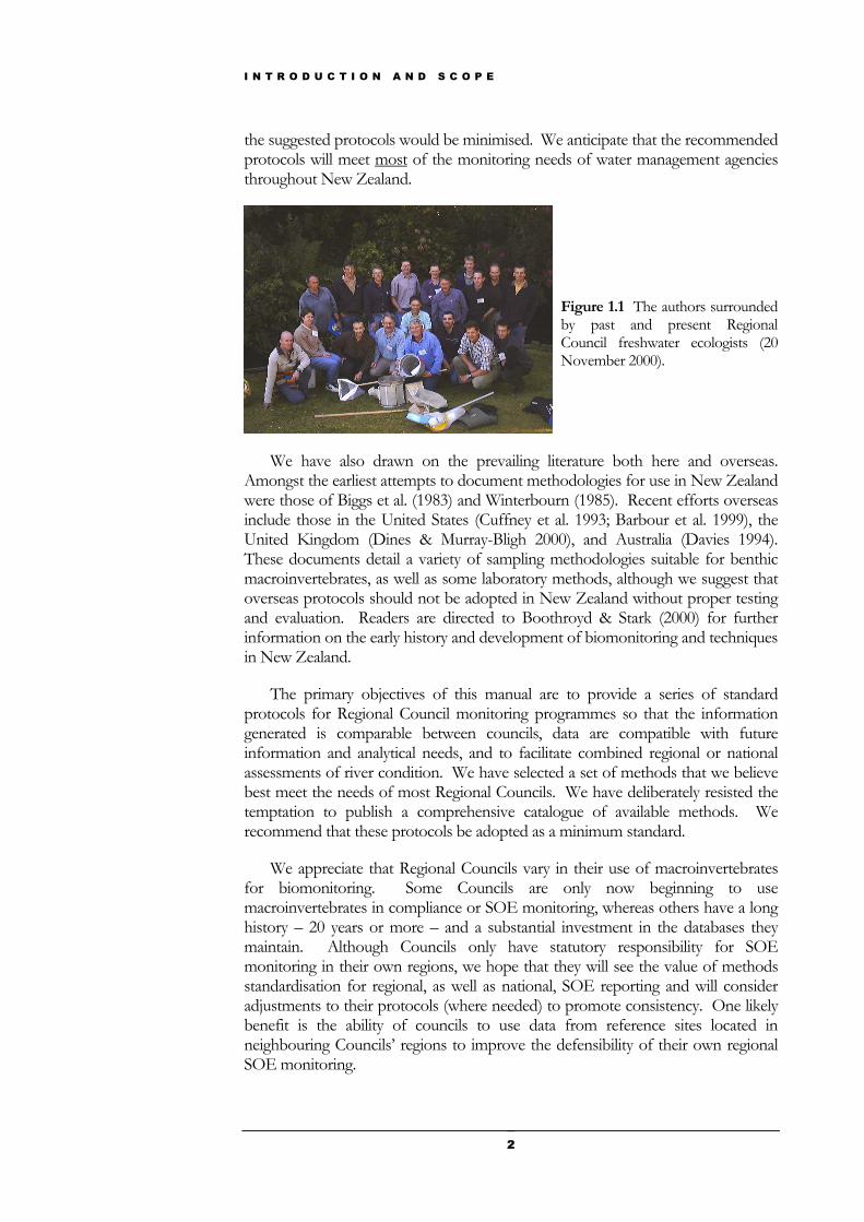
A hands-on demonstration of sampling methods, attended by the authors and at least 15 Regional Council biologists, was held on 20 November 2000 beside the Avon River near the Staff Club of the University of Canterbury (Figure 1.1). By sharing ideas and discussing issues we hoped that any barriers to the adoption of
Chapter
1 T
I N T R O D U C T I O N A N D S C O P E
2
the suggested protocols would be minimised. We anticipate that the recommended protocols will meet most of the monitoring needs of water management agencies throughout New Zealand.
Figure 1.1 The authors surrounded by past and present Regional Council freshwater ecologists (20 November 2000).
We have also drawn on the prevailing literature both here and overseas. Amongst the earliest attempts to document methodologies for use in New Zealand were those of Biggs et al. (1983) and Winterbourn (1985). Recent efforts overseas include those in the United States (Cuffney et al. 1993; Barbour et al. 1999), the United Kingdom (Dines & Murray-Bligh 2000), and Australia (Davies 1994). These documents detail a variety of sampling methodologies suitable for benthic macroinvertebrates, as well as some laboratory methods, although we suggest that overseas protocols should not be adopted in New Zealand without proper testing and evaluation. Readers are directed to Boothroyd & Stark (2000) for further information on the early history and development of biomonitoring and techniques in New Zealand.
The primary objectives of this manual are to provide a series of standard protocols for Regional Council monitoring programmes so that the information generated is comparable between councils, data are compatible with future information and analytical needs, and to facilitate combined regional or national assessments of river condition. We have selected a set of methods that we believe best meet the needs of most Regional Councils. We have deliberately resisted the temptation to publish a comprehensive catalogue of available methods. We recommend that these protocols be adopted as a minimum standard.
We appreciate that Regional Councils vary in their use of macroinvertebrates for biomonitoring. Some Councils are only now beginning to use macroinvertebrates in compliance or SOE monitoring, whereas others have a long history – 20 years or more – and a substantial investment in the databases they maintain. Although Councils only have statutory responsibility for SOE monitoring in their own regions, we hope that they will see the value of methods standardisation for regional, as well as national, SOE reporting and will consider adjustments to their protocols (where needed) to promote consistency. One likely benefit is the ability of councils to use data from reference sites located in neighbouring Councils’ regions to improve the defensibility of their own regional SOE monitoring.
I N T R O D U C T I O N A N D S C O P E
3
In October 2000, a questionnaire was sent to all Regional Council biologists and selected biologists from universities, research institutes, Department of Conservation, and independent consultants in New Zealand (Appendix A). The recommended methods were developed from the responses, and the respondents reviewed a draft of this manual in mid-September. A final draft of the manual was circulated for comment amongst members of the New Zealand Macroinvertebrate Working Group in mid-November 2001.
The respondents to the initial questionnaire identified three main sampling objectives:
• State of the Environment monitoring (SOE) • Assessment of Environmental Effects (AEE) • Compliance monitoring
Scope This protocols manual includes:
• sample collection methods • sample processing protocols • quality control procedures • advice on the level of taxonomic resolution • advice on sample storage
This manual is not a guide to compliance or SOE monitoring programme design and does not include advice on:
• study design • site selection • biomonitoring indices • data analytical techniques • data interpretation
It is essential that users of these protocols have a reasonable understanding of freshwater ecology and some training or experience in stream macroinvertebrate sampling procedures. It is also the users’ responsibility to define the objectives of their investigation and to ensure that the sampling and sample processing methods that they employ will provide data that meet their information requirements. An integral part of sound study design is a clear understanding of how the data collected will be analysed, interpreted and reported.
The methods outlined in this document are recommended for use in wadeable running waters - the stream and river types conventionally selected for biomonitoring. The techniques described here may be suitable for other
I N T R O D U C T I O N A N D S C O P E
4
freshwater habitats such as such as wetlands, lake shores and ponds. However adequate sampling of these habitats frequently requires alternative techniques, which are not described here. Similarly, field-sampling methods described here generally will not be appropriate for deeper, swifter rivers (i.e., non-wadeable) where the use of grab samplers, SCUBA and boats may be required.
Procedures necessary to produce quantitative and relative abundance macroinvertebrate data are presented in detail, including field collection, preservation, processing, and QC for sample processing.1
Guiding principles Use of macroinvertebrates for biomonitoring
The use of aquatic macroinvertebrates in biomonitoring has focussed traditionally on their utility as indicators of water quality, as evidenced by the number of times the term ‘water quality’ features in the titles of references cited in this document. Water quality is defined here as the physical (e.g., clarity, temperature) and chemical (e..g., nutrients, BOD) characteristics of surface waters. In fact, many of the metrics commonly applied to macroinvertebrate data (e.g., %EPT, MCI) were developed as indices of water quality degradation (i.e., organic enrichment).
Although the use of aquatic macroinvertebrates for assessments of water quality arose from the historic focus on water pollution related to human health and safety, macroinvertebrates are being used increasingly to assess the ‘health’ of aquatic ecosystems (along with other physical, chemical, and biological measures). Although the term ‘stream health’ remains somewhat ill-defined, and how best to measure it is uncertain, it is an appealing concept easily understood by laypersons, at least with respect to macroinvertebrate-based SOE monitoring. However, it is beyond the scope of this document to provide guidance on the best methods to assess ‘stream ecosystem health’.
Water quality remains a major focus of interest for the general public, politicians, user groups and industry. Current SOE programmes retain, at least in part, a valuable water quality assessment component. In these protocols we have focussed on the use of aquatic macroinvertebrates for assessments of water quality. We have deliberately selected habitats, such as riffles, where macroinvertebrates most sensitive to water quality degradation normally are present, and where the absence of pollution-sensitive groups has proven to be a useful indicator of environmental condition. However, certain adverse effects on stream condition may not always be best detected by sampling macroinvertebrate communities in riffle habitats, or by sampling macroinvertebrates at all. Sedimentation effects, for example, may appear first in pools and runs, and dramatic changes in riparian cover may foreshadow subsequent changes to instream biological communities.
1 The hard-copy of this manual was supplied with the protocols on plastic-laminated sheets.
I N T R O D U C T I O N A N D S C O P E
5
Whenever aquatic macroinvertebrates are used in biomonitoring, it is essential to provide a clear statement at the outset of the objectives of the work. Different objectives (e.g., water quality, stream ‘health’, sedimentation) may require different approaches (e.g., different sampling methods, habitats, measures, sample processing and analyses). We suggest that where deviations from the recommended methods are required they should be well documented.
Hard- and Soft-bottomed Streams Separate protocols are provided for hard-bottomed and soft-bottomed
streams. This separation reflects significant differences in the morphology and community composition of these respective stream types, and recognises that different methods are required if sample collection and processing are to be cost-effective. It is our intention that this separation will help focus attention on soft-bottom streams as distinct entities, following recommendations of the New Zealand Macroinvertebrate Working Group (MfE 1999), and will reduce the temptation for inappropriate comparisons between hard and soft-bottomed streams.
A hard-bottomed stream is one where the substrate is dominated by particles of gravel size or greater (i.e., <50% of the bed is made up of sand/silt). Riffle habitats normally are common in these streams, reflecting a reasonable stream gradient. In contrast, soft-bottomed streams are usually low-gradient, and dominated by glide/pool habitats. Gravel, cobble and boulder substrates are rare or absent in these streams and sand/silt/mud/clay dominate the streambed. Macrophytes often dominate in unshaded reaches, whereas soft-bottomed streams in forested areas often have accumulations of woody debris that form stable, productive habitat for macroinvertebrates.
In both stream types, the principal goal of sampling is to collect a macroinvertebrate sample that is representative of the site, and provides information that meets the study objectives. Experience suggests that a single D-net sample from an area from approximately 0.6 – 1.0 m2 of riffle habitat will provide a representative sample in most hard-bottomed streams.
Because of the paucity of productive habitat in many soft-bottomed streams the situation is less straightforward. Published data on macroinvertebrate communities in minimally disturbed soft-bottomed streams are sparse due to the high degree of human modification of lowland areas in New Zealand, and the practical difficulty of sampling these types of streams. Collier et al. (1998), in a study of 20 lowland, soft-bottomed Waikato streams, found a median benthic macroinvertebrate density (1334 m-2) - half that reported for hard-bottomed streams throughout New Zealand (2784 m-2; Scarsbrook et al. 2000). In addition, Collier et al. (1998) found that woody debris, where present, was a particularly important substrate, particularly for Ephemeroptera, Plecoptera and Trichoptera. In a recent study, of minimally disturbed soft-bottom streams in the Auckland region, it was found that macroinvertebrate densities were less than 10% of those in hard-bottomed streams (J. R. Maxted, unpublished data). Theses studies suggest that collection of ‘representative samples’ from soft-bottomed streams, especially minimally disturbed ones, may require greater effort than for hard-bottomed
I N T R O D U C T I O N A N D S C O P E
6
streams. In addition, the importance of woody debris as a stable substrate suggests it should be included in sampling protocols where it is present.
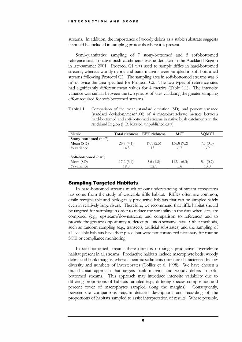
Semi-quantitative sampling of 7 stony-bottomed and 5 soft-bottomed reference sites in native bush catchments was undertaken in the Auckland Region in late-summer 2001. Protocol C1 was used to sample riffles in hard-bottomed streams, whereas woody debris and bank margins were sampled in soft-bottomed streams following Protocol C2. The sampling area in soft-bottomed streams was 6 m2 or twice the area specified for Protocol C2. The two types of reference sites had significantly different mean values for 4 metrics (Table 1.1). The inter-site variance was similar between the two groups of sites validating the greater sampling effort required for soft-bottomed streams.
Table 1.1 Comparison of the mean, standard deviation (SD), and percent variance (standard deviation/mean*100) of 4 macroinvertebrate metrics between hard-bottomed and soft-bottomed streams in native bush catchments in the Auckland Region (J. R. Maxted, unpublished data).
Metric Total richness EPT richness MCI SQMCI Stony-bottomed (n=7) Mean (SD) 28.7 (4.1) 19.1 (2.5) 136.8 (9.2) 7.7 (0.3) % variance 14.3 13.1 6.7 3.9 Soft-bottomed (n=5) Mean (SD) 17.2 (3.4) 5.6 (1.8) 112.1 (6.3) 5.4 (0.7) % variance 19.8 32.1 5.6 13.0
Sampling Targeted Habitats In hard-bottomed streams much of our understanding of stream ecosystems
has come from the study of wadeable riffle habitat. Riffles often are common, easily recognisable and biologically productive habitats that can be sampled safely even in relatively large rivers. Therefore, we recommend that riffle habitat should be targeted for sampling in order to reduce the variability in the data when sites are compared (e.g., upstream/downstream, and comparison to reference) and to provide the greatest opportunity to detect pollution sensitive taxa. Other methods, such as random sampling (e.g., transects, artificial substrates) and the sampling of all available habitats have their place, but were not considered necessary for routine SOE or compliance monitoring.
In soft-bottomed streams there often is no single productive invertebrate habitat present in all streams. Productive habitats include macrophyte beds, woody debris and bank margins, whereas benthic sediments often are characterised by low diversity and numbers of invertebrates (Collier et al. 1998). We have chosen a multi-habitat approach that targets bank margins and woody debris in soft-bottomed streams. This approach may introduce inter-site variability due to differing proportions of habitats sampled (e.g., differing species composition and percent cover of macrophytes sampled along the margins). Consequently, between-site comparisons require detailed descriptions and recording of the proportions of habitats sampled to assist interpretation of results. Where possible,
I N T R O D U C T I O N A N D S C O P E
7
between-site comparisons (e.g., upstream/ downstream of a discharge) should be made across similar habitats.
Sampling of invertebrates associated with determined weights of aquatic macrophytes provides a simple quantitative method in soft-bottomed streams where macrophytes are present, and this is recommended where replicated estimates of invertebrate densities are required (Protocol C4).
While the protocols presented here target certain habitat types, we suggest that other less common habitats should also be considered if time and budget allows. For example, in soft-bottomed streams there may be occasional accumulations of coarse substrates forming riffles, and runs or woody debris dams may be found in hard-bottomed streams. These habitats, while sometimes rare, may hold ecologically important information that may help with the description of site condition. If possible the fauna in such should be described, with samples kept separate from the principal site sample.
Woody debris often is not present in open-channel soft-bottomed streams (e.g., rural streams), and may be sparse in well-shaded streams, especially those with sufficient gradient to flush-out woody debris during storms. Woody debris should be sampled whenever it is encountered in soft-bottomed streams due to its importance as a substrate for pollution sensitive groups.
A recent review of macroinvertebrate monitoring methods used by USA state agencies indicated that most (63.4% or 52/82) sampling programmes targeted a single habitat, with riffles (25.6%) or riffles + runs (24.4%) preferred (Carter & Resh 2001). However, 23% of programmes attempted to sample all available habitats, usually in proportion to their occurrence. While sampling multiple habitats in proportion to their occurrence is likely to collect a greater variety of taxa, Carter & Resh (2001) considered that it was more difficult to standardise than collecting from a single habitat and could compromise between-site comparisons. This supports our decision to sample single habitats for most protocols (Protocols C1, C3 & C4), and to propose a multi-habitat approach for semi-quantitative sampling of soft-bottomed streams (Protocol C2) simply because there is no single productive habitat in common to all such sites.
Standardisation of sampling effort During the development of these protocols much discussion was concerned
with standardisation of semi-quantitative sampling effort. Procedures in current use by Regional Councils include sampling effort based on area, time and volume of collected material. Regardless of the procedure used it is vital to maintain consistency in the effort expended for each sample. Following the advice of Elliott (1977) and Winterbourn (1985) we recommend a pre-defined area approach. Sampling by area reduces the likelihood of variation in data due to differences in the enthusiasm of field staff, and is consistent with protocols used by Co-operative Research Centres (CRCs) in Australia and the US EPA (Barbour et al 1999).
I N T R O D U C T I O N A N D S C O P E
8
Sample size Cost-effective biomonitoring depends upon the collection of appropriately
sized macroinvertebrate samples. Samples must be large enough to represent communities at the site adequately, but not so large that they are too time-consuming to process. Given the high spatial and temporal variability in macroinvertebrate communities and variability introduced by different sampling personnel, it is not easy to give specific and unambiguous guidance on sample size.
Stark (1998) found that four Surber samples (0.1 m2 area, 0.5 mm mesh) provided estimates of MCI similar in precision (just over ± 10%) to a single D-net sample (0.5 mm mesh) collected from an area of 0.3 – 0.6 m2. Three D-net samples or 8 Surber samples were required to achieve precision of around ± 10% for the SQMCI and QMCI variants respectively.
This suggests that representative macroinvertebrate sample from a hard-bottomed stream can be obtained using a D-net (or similar) by sampling approximately 0.6 – 1.0 m2 of streambed. Depending on the aims of an investigation and the precision required, replicate samples might need to be collected or sampling repeated on several occasions. For example, if macroinvertebrate taxon richness or densities seem low when collecting samples, collection of additional samples of the standard effort is preferred rather that simply increasing the sample size. Note that replicate samples must be processed separately and should not be composited. Quantitative sampling using Surber or Hess samplers will require sample replication if estimates of variance are required (e.g., for statistical techniques such as ANOVA), and to obtain a representative taxa list for a site.
In soft-bottomed streams we recommend a level of effort that is approximately three times that in hard-bottomed streams (i.e., a sample of approximately 3 m2). At present we know far less about the ecology of soft-bottomed streams than we do about hard-bottomed streams. However, based on these limited data, and our collective experience, we believe that a sample of 3 m2 should provide a representative sample from most soft-bottomed streams. Samples collected in the Auckland region showed that reducing the sample size from 6 m2 to 3 m2 had no effect on most metrics. Richness metrics, however, increased with sample size up to 18 m2, indicating that they should be used with caution in soft-bottomed streams (J.R. Maxted, unpublished data). These data also suggested that some minimally disturbed soft-bottomed sites may have very low invertebrate densities (< 100 individuals per 3 m2 sampled), and that replicate samples may be needed to characterise macroinvertebrate community composition reliably.
Mesh Size By convention, the term macroinvertebrates refers to invertebrates retained by
a 0.5 mm net or sieve. Whereas a smaller mesh size may be required for detailed studies of life history, secondary production, or recolonisation, Winterbourn (1985) concluded that 0.5 mm mesh was sufficient for most biomonitoring purposes. We prescribe the use of a 0.5 mm mesh net in all sampling protocols in this manual. Samplers using 0.5 mm mesh will collect much less fine sediment, will be less
I N T R O D U C T I O N A N D S C O P E
9
prone to clogging, are easier to use in faster water, and will collect samples that are quicker to process than samplers using finer mesh.
A recent review of macroinvertebrate monitoring methods used by USA state agencies indicated that 0.5 mm mesh was the most common mesh size (used by 38.3% of programmes). The 0.5 – 0.6 mm range covered 80.2% of all programmes. Only 2.4% used finer (0.35 & 0.425 mm) mesh (Carter & Resh 2001). Carter & Resh (2001) noted, however, that research studies (as opposed to monitoring) often used finer mesh.
Sample Preservation Samples should be preserved for later identification in the laboratory.
Winterbourn et al. (2000) provide a detailed discussion of preservation. The fluid most commonly used for preservation of aquatic macroinvertebrates is ethyl alcohol (ethanol). However, preservation is enhanced if certain other substances, such as formaldehyde, are added to the alcohol, although these invariably are unpleasant or hazardous substances (Table 1.2).
We recommend the use of ethanol-based preservatives (70 – 90% aqueous solution) because they are comparatively safe (Table 1.2). “Ethanol solution” (e.g., Mobil SDA-3A) – denatured alcohol comprising approximately 99.8% ethanol and 0.2% methanol – available from some service stations - is a suitable and much cheaper alternative. Isopropyl alcohol and methanol have similar preservation properties to ethanol and also are cheaper, although more toxic (Table 1.2). Direct contact with methanol should be avoided as it is absorbed through the skin.
Table 1.2 Workplace exposure standards for commonly used preservatives (OSH 2001).
Workplace Exposure Standards (Threshold Limit Value)
TWA(a) STEL(b) Chemical Ppm(c) mg/m3(d) ppm Mg/m3 Ethanol 1,000 1,880 - - Formaldehyde 1 1.2 - - Isopropyl alcohol 400 983 500 1,230 Methanol 200 262 250 328
(a) Time-Weighted Average concentration for a normal 8-hour work day 40-hour work week, to which nearly all workers may be repeatedly exposed, day after day, without adverse effect.
(b) Short-Term Exposure Limit – the concentration to which workers can be exposed continuously for a short period of time without suffering from irritation, chronic or irreversible tissue damage or narcosis of sufficient degree to increase the likelihood of accidental injury, impair self-rescue or materially reduce work efficiency, and provided that the daily TLV-TWA is not exceeded.
(c) Parts of vapour or gas per million of contaminated air by volume at 25 oC and 760 torr. (d) Milligrams of substance per cubic metre of air.
However, alcohol-based preservatives do remove the bright colours of larvae and the preservative becomes diluted by the body fluids of the animals in the sample. Samples containing large quantities of organic material (including macrophytes, periphyton, wood, leaves etc.) need very generous quantities of
I N T R O D U C T I O N A N D S C O P E
10
preservative if macroinvertebrates are to be well preserved. If samples are to be kept for more than a week or two before processing, the preservative should be replaced to maintain the preservative concentration. This is most important for organic-rich samples.
Addition of 1 – 4% formalin to ethanol improves the effectiveness of ethanol as a preservative. Formalin (formaldehyde) is a fixative that helps to maintain the colour and shape of macroinvertebrates. Full safety precautions (rubber gloves, adequate fume extraction or ventilation) should be observed if it is used (OSH 1992, 1999). Formaldehyde is a sensitiser and is suspected of being a human carcinogen. We do not recommend the use of formalin for Regional Council monitoring, unless properly equipped laboratories are available, and all staff are fully protected.
While macroinvertebrate biomonitoring seldom involves determination of macroinvertebrate biomass (either dry- or wet-weights), alcohol-based preservatives generally are unsuitable for these purposes. Donald & Paterson (1977) recommended 10% formalin (4% formaldehyde) prepared with filtered habitat water. However, Howmiller (1972) found that dry weight estimates obtained 55 days following preservation in 10% formalin, 70% ethanol, or 70% isopropanol could be only 50 – 60% of those obtained from unpreserved specimens. In our view, all preservatives are likely to cause significant weight loss and no general recommendation for preservatives suitable for biomass studies can be made. In general, we recommend that samples that are to be assessed for biomass should be frozen, rather than preserved.
Sample Processing Our survey of current Regional Council practices (Appendix A) indicated that
three methods for macroinvertebrate sample processing are widely used:
• Full counts (with the option of sub-sampling abundant taxa) • Fixed count (with scan for rare taxa) • Coded abundance
All three methods provide for the compilation of species lists and the calculation of many biotic metrics commonly used to indicate stream health. The key difference between the methods centres on the way in which abundances of macroinvertebrates in samples are assessed.
Full counts provide the most precise estimate of the abundances of individual taxa in a sample. For samples collected from a known area (quantitative sample), the density of organisms at a site can be estimated (i.e., number m-2) and accurate percentage community compositions can be determined.
Fixed count protocols involve the systematic identification and counting of a pre-defined number of animals in a sample. This normally is 100, 200, or 300 animals. A scan for rare taxa is required to complete the species list, but it is important to realise that these “rare” taxa play no part in the calculation of metrics
I N T R O D U C T I O N A N D S C O P E
11
that require percentage composition data. Fixed count procedures can provide good approximations of percentage community composition provided sufficient animals are counted.
Coded abundance sample processing protocols provide an approximation of the actual abundance of individual taxa in the sample by placing each species into an abundance category (rare, common, abundant, etc.). This method is dependent on sampling effort, since the abundance of individual species increases with the area sampled.
In our view, both fixed count and coded abundance approaches are sufficient to fulfil the current information needs of Regional Councils.
Quality Assurance and Quality Control Quality Assurance (QA) is the measurement and control of errors from
whatever source (Dines & Murray-Bligh 2000). Quality control (QC) refers to inspections or tests, an integral part of QA procedures, which determine whether or not a product or service meets the required standard.
Although these protocols do not represent a formal or accredited QA system, we believe that the existence of well-documented standard methods, including QC procedures, should promote the production of accurate, reliable and consistent macroinvertebrate data at all times. We believe that the adoption of these protocols will confer considerable value and reliability on the information gained from both new and existing programs.
Quality Assurance programmes exist for biological monitoring programmes using rapid assessment protocols in the UK (Dines & Murray-Bligh 2000), USA (Plafkin et al. 1989, Cuffney et al. 1993), and Australia (Humphrey et al. 2000). These methods form the basis of the protocols suggested here. QC requirements recommended here focus on the two most likely sources of error: sorting and taxonomy. We have attempted to make the procedures as simple and straightforward as possible without adding substantially to effort and expense. Generally, the QC steps we are proposing add 10 - 15%, at most, to the cost of the data.
In general, we recommend QC procedures that involve re-examination of 10% of samples selected at random. The second taxonomist will be provided with the results obtained by the original taxonomist to check the identifications and counts or relative abundances. We considered whether the second taxonomist should check the samples independently (i.e., without having the results from the first sorter) but decided that a comparison of results would be more cost-effective and educational. For example, the second taxonomist can explain any differences in identifications that arise, rather than this reconciliation requiring an additional stage. Furthermore, the condition of macroinvertebrates in samples tends to deteriorate with handling, so the comparative approach is less likely to disadvantage the second sorter. If two equally-experienced taxonomists disagree on an identification then a third opinion should be sought from an agreed independent expert.
I N T R O D U C T I O N A N D S C O P E
12
The responsibility for QC assessment rests with the organisation that collected the samples, and should involve an organisation independent of the one that produced the original data. All data should be checked for QC and accompanied by a QC report. The QC report does not need to be lengthy but adequate to document the steps taken to ensure data quality.
However, it is not our expectation that formal QC will necessarily be carried out on all sampling programmes at all times. Rather, we suggest that QC effort be directed at significant SOE, AEE or compliance monitoring programmes periodically (e.g., once every three years), or following a change of personnel involved in macroinvertebrates sorting and identification. Thus we anticipate that a QC report noting that the personnel who sorted the samples had recently passed QC on a previous project would suffice, but an outdated testimonial (say > 3 years old), or the use of personnel of unproven capability, would not be acceptable evidence of quality assured data. Where casual personnel are used for sorting and identification a QC report would be expected for each significant project.
We urge all users of this manual to consider seriously the implementation of appropriate recommended QC procedures whether a protocol is used in full or in part. We recognise that QC, especially if diligently applied, comes with an additional cost in time and resources, especially money, not to mention goodwill. Nevertheless, properly applied, the recommended QC protocols for sample processing will provide greater confidence in the data produced.
Finally, the best efforts for ensuring that sample processing and taxonomy are undertaken to a high standard are futile if valuable data are not recorded correctly. Errors can occur when entering data on to the computer where it may be stored in spreadsheets or in a database. Although we have not specified QC protocols for data entry or specified how data should be managed, we urge those who generate data to pay particular attention to data entry and data security and to adopt procedures involving independent checking wherever possible.
Transition from Existing Methods Although the recommended protocols are based on methods in current usage
(Appendix A) several Regional Councils have considerable investment in existing macroinvertebrate data collected, or processed, using methods that differ slightly from those proposed in this manual. Understandably, there may be some reluctance to adopt the new protocols if it results in a discontinuity in the data time series.
The proposed protocols should be regarded as minimum standards. We recommend that Regional Councils adopt these protocols to provide greater national consistency and to facilitate scientifically defensible national SOE reporting. In most cases, the recommended methods are likely to prove most cost-effective than their present methods! We can see no reasons why those Councils that have only recently embarked on SOE monitoring (or have not yet done so) should not adopt the recommended protocols.
I N T R O D U C T I O N A N D S C O P E
13
Councils with extensive existing data and concerns about the consequences of change could undertake comparisons to ensure that their methods exceed the standards and provide compatible data. For example, a Council considering adopting a new sampling protocol could collect the majority of their samples using their existing method and could use the appropriate recommended protocol to collect additional samples from 5 – 10% of their sites. They could then compare the data obtained using the two methods to determine whether their protocol collects compatible data (to justify retaining the status quo) or whether the change in sampling method will affect data quality significantly.
Selecting a Protocol The objectives and information needs of a study should determine the
methods to be used. What we have provided in this manual are methods that should be appropriate for most Regional Council monitoring objectives, but the onus is on the user to ensure that their chosen study design, sampling and sample processing procedures are appropriate to their needs. This manual is focused on the field and laboratory, and quality control components of State of the Environment (SOE), Assessment of Environmental Effects (AEE) and Consent Compliance monitoring.
For SOE monitoring programmes we have assumed that the study objectives will be to provide biological information on a selection of streams in a region, and allow for the comparison of sites through time. This approach obviously requires the sampling of as many sites as possible, from reference through to impacted condition. We anticipate that sampling will be on a seasonal basis at best, but is more likely to be annual or semi-annual. Given these constraints, it is unlikely that quantitative sampling will be cost-effective, and semi-quantitative methods provide an appropriate alternative. In comparison, AEE work and compliance monitoring may require more detailed site comparisons where the additional information gained from quantitative sampling may be justified.
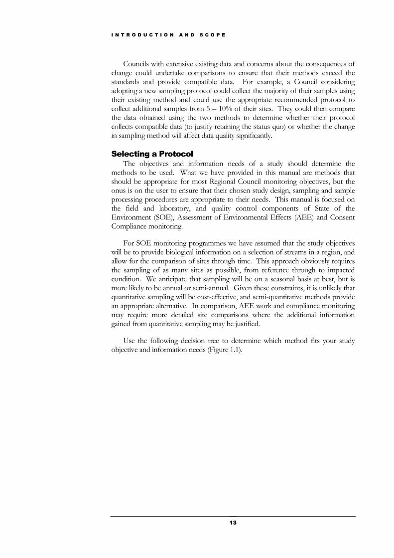
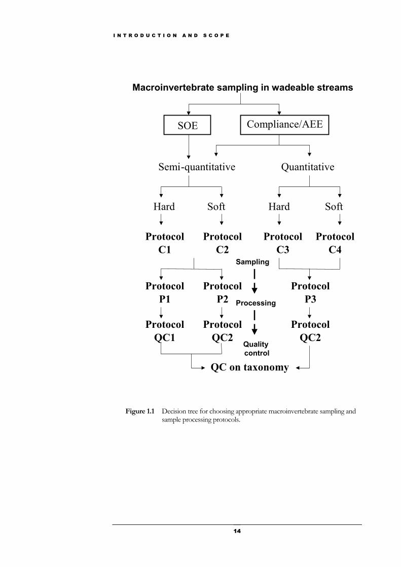
Use the following decision tree to determine which method fits your study objective and information needs (Figure 1.1).
I N T R O D U C T I O N A N D S C O P E
14
Macroinvertebrate sampling in wadeable streams
SOE Compliance/AEE
Semi-quantitative Quantitative
Hard Soft Hard Soft
ProtocolC1
ProtocolC2
ProtocolC3
ProtocolC4
ProtocolP1
ProtocolP2
ProtocolP3
ProtocolQC1
ProtocolQC2
ProtocolQC2
QC on taxonomy
Sampling
Processing
Qualitycontrol
Figure 1.1 Decision tree for choosing appropriate macroinvertebrate sampling and sample processing protocols.
S A M P L E C O L L E C T I O N
15
Sample Collection
Introduction e provide four protocols for collecting macroinvertebrate samples: two semi-quantitative protocols (for hard (Protocol C1) and soft-bottomed streams (Protocol C2)), and two quantitative protocols (for hard substrates (Protocol C3) and macrophyte beds (Protocol C4).
In order to promote standardisation, after surveying methods in current use (Appendix A), we have deliberately provided only one sampling protocol for each purpose/habitat. Although we see benefits from Regional Councils adopting these protocols exactly as specified, we accept that there may be some reluctance amongst councils with existing datasets, due to concerns that the integrity of their data may be compromised. In such cases the proposed protocol/s could be run in parallel with existing methods to determine whether such concerns are valid.
The recommended protocols may be regarded as a minimum standard. We believe they will provide more reliable estimates of biotic indices than smaller samples obtained with less effort and will be more cost-effective than some sampling protocols in current use.
It is beyond the scope of this document to provide guidance on sampling programme design, site selection, and sample replication, but it is essential that such matters be considered together with the aims of the investigation to ensure that an appropriate sampling protocol is used. It is worth emphasising that even the highest standards of sample collection and processing performance will not compensate for a poorly designed sampling programme. The recommended protocols provide standard methods for collection (and processing) of single samples. It is up to the investigator to determine whether the study objectives can be satisfied by collection of single samples or if sample replication is required for semi-quantitative sampling. Quantitative sampling programmes will require replicate samples where estimates of variance in density are required.
Sampling equipment Equipment requirements for the proposed macroinvertebrate sampling
protocols are relatively modest. Some items are essential, whereas, other equipment is optional depending upon whether or not additional information on
Chapter
2 W
S A M P L E C O L L E C T I O N
16
the characteristics of the sampling site is recorded when macroinvertebrate sampling is undertaken.
Essential equipment includes:-
• Waders or gumboots, depending on depth of the streams. • D-framed handnet (D-net) (or similar) or Surber sampler (0.5 mm mesh) • White tray or 10 litre bucket • Sieve or sieve bucket (0.5 mm mesh) • Plastic sample containers (usually 500 – 1000 ml volume) • Preservative • Sample container labels • Waterproof marker pen and pencil • Field notebook or field data record sheets
Additional sampling information The site location (including map- or GPS-reference), sampling date, sampling
time, and name of personnel undertaking sampling should also be recorded. A site photograph is useful and water quality or stream habitat measurements are essential for subsequent interpretation of biological data. At the very least, assessments of substrate composition, riparian vegetation, stream width and depth, temperature, conductivity, dissolved oxygen, and periphyton community composition should be considered. Not only will this improve the ability to interpret macroinvertebrate data, but it will also provide valuable information for future analyses (e.g., construction of predictive models). The selection of which physico-chemical or habitat parameters to measure should be dictated by the study aims, and is not addressed in these protocols.
Collection Protocols Two methods for hard-bottomed streams (Protocols C1 & C3) and two
methods for soft-bottomed streams (Protocols C2 & C4) are presented.
A stream is considered hard-bottomed when gravel, cobble, boulder and bedrock substrates dominate (>50% by area) the streambed. Shallow riffle substrate is common in these streams, and provides a consistent, easily recognisable, and biologically productive habitat for sampling. In contrast, no single substrate is found over the full range of stream types and levels of disturbance in soft-bottomed streams. Therefore, a variety of stable substrates (e.g., bank margins, woody debris and macrophytes) are recommended for sampling in soft-bottomed streams. A soft-bottomed streambed may be dominated by sand, silt, mud, clay, macrophytes, and woody debris, whereas gravel, cobble, boulder and bedrock substrates may be rare or absent. The proportions of each habitat sampled should be recorded.
S A M P L E C O L L E C T I O N
17
Where both hard and soft substrate types are found at a site, sampling should concentrate on the habitat type that is most representative of the stream reach being sampled. Alternatively, samples should be collected and processed separately from each habitat type.
Protocol C1 – Hard-bottomed, semi-quantitative. Protocol C1 is designed for collection of semi-quantitative macroinvertebrate
data. It is most appropriate for riffle habitat in stony streams, but may also be used, less effectively, in deeper water. It is suitable for use with both relative abundance and fixed count processing protocols (Protocols P1 & P2), and provides data suitable for SOE and compliance monitoring and AEE’s where quantitative data are not considered necessary. A variety of species richness and relative abundance metrics and multivariate analyses can be calculated.
A D-net (Cuffney et al. 1993) with 0.5 mm mesh is recommended for Protocol C1. Carter & Resh (2001) noted that D-nets were the most commonly used sampling device for biomonitoring by state agencies in the USA (being used in 35.6% of programmes). In fact, 64.5% of programmes used some form of kick-type sampler (cf., fixed quadrat like Surber 8.9%, artificial substrates 13.3%, grabs 2.2%) (Carter & Resh 2001). Although D-nets are suitable for collecting samples from a wide range of habitat types in hard-bottomed streams (from sand through to boulders or bedrock), sampling in riffle habitat is recommended to minimise variability and improve the validity of between-site or temporal comparisons.
The shape (e.g., D, rectangular, triangular, or circular) and size of the net can vary provided it has the proper mesh size although a D-net 30 – 40 cm wide along the base is recommended. If the net is too narrow, the current may carry dislodged macroinvertebrates and debris past the net rather than into it. The net will remain serviceable for longer if the mesh is attached to the frame by a sleeve of tough calico or plastic, or has a metal or plastic-covered leading edge. The net should be at least 50 cm long to minimise clogging and backflow around the mouth.
To operate a D-net, the substratum (organic and/or inorganic) must be disturbed immediately upstream of the net. The distance depends on the flow regime, but generally should be less than 0.5 metres from the mouth of the net.
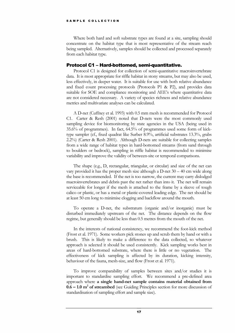
In the interests of national consistency, we recommend the foot-kick method (Frost et al. 1971). Some workers pick stones up and scrub them by hand or with a brush. This is likely to make a difference to the data collected, so whatever approach is selected it should be used consistently. Kick sampling works best in areas of hard-bottomed substrate, where there is little or no vegetation. The effectiveness of kick sampling is affected by its duration, kicking intensity, behaviour of the fauna, mesh-size, and flow (Frost et al. 1971).
To improve comparability of samples between sites and/or studies it is important to standardise sampling effort. We recommend a pre-defined area approach where a single hand-net sample contains material obtained from 0.6 – 1.0 m2 of streambed (see Guiding Principles section for more discussion of standardisation of sampling effort and sample size).
S A M P L E C O L L E C T I O N
18
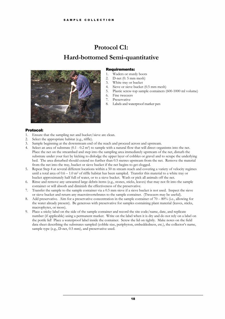
Protocol C1:
Hard-bottomed Semi-quantitative
Requirements: 1. Waders or sturdy boots 2. D-net (0. 5 mm mesh) 3. White tray or bucket 4. Sieve or sieve bucket (0.5 mm mesh) 5. Plastic screw-top sample containers (600-1000 ml volume) 6. Fine tweezers 7. Preservative 8. Labels and waterproof marker pen
Protocol: 1. Ensure that the sampling net and bucket/sieve are clean. 2. Select the appropriate habitat (e.g., riffle). 3. Sample beginning at the downstream end of the reach and proceed across and upstream. 4. Select an area of substrate (0.1 - 0.2 m2) to sample with a natural flow that will direct organisms into the net.
Place the net on the streambed and step into the sampling area immediately upstream of the net, disturb the substrate under your feet by kicking to dislodge the upper layer of cobbles or gravel and to scrape the underlying bed. The area disturbed should extend no further than 0.5 metres upstream from the net. Remove the material from the net into the tray, bucket or sieve bucket if the net begins to get clogged.
5. Repeat Step 4 at several different locations within a 50 m stream reach and covering a variety of velocity regimes until a total area of 0.6 – 1.0 m2 of riffle habitat has been sampled. Transfer this material to a white tray or bucket approximately half full of water, or to a sieve bucket. Wash or pick all animals off the net.
6. Rinse and remove any unwanted large debris items (e.g., stones, sticks, leaves) that may not fit into the sample container or will absorb and diminish the effectiveness of the preservative.
7. Transfer the sample to the sample container via a 0.5 mm sieve if a sieve bucket is not used. Inspect the sieve or sieve bucket and return any macroinvertebrates to the sample container. (Tweezers may be useful).
8. Add preservative. Aim for a preservative concentration in the sample container of 70 – 80% (i.e., allowing for the water already present). Be generous with preservative for samples containing plant material (leaves, sticks, macrophytes, or moss).
9. Place a sticky label on the side of the sample container and record the site code/name, date, and replicate number (if applicable) using a permanent marker. Write on the label when it is dry and do not rely on a label on the pottle lid! Place a waterproof label inside the container. Screw the lid on tightly. Make notes on the field data sheet describing the substrates sampled (cobble size, periphyton, embeddedness, etc.), the collector’s name, sample type (e.g., D-net, 0.5 mm), and preservative used.
S A M P L E C O L L E C T I O N
19
Protocol C2 – Soft-bottomed, semi-quantitative Protocol C2 is the soft-bottomed stream equivalent of Protocol C1. It is
suitable for use with both relative abundance and fixed count processing protocols (Protocols P1 & P2), and provides data suitable for SOE and compliance monitoring and AEE’s where quantitative data are not considered necessary. A variety of species richness and relative abundance metrics and multivariate analyses can be calculated.
There is no single substrate that is suitable for the collection of macroinvertebrates in most soft-bottomed streams. Woody debris is considered the soft-bottomed stream equivalent to productive riffle habitat targeted for sampling in hard-bottomed streams, but woody debris is not found in all soft-bottomed streams. Similarly, aquatic macrophytes often dominate open channel streams, but are rare or absent in well-shaded soft-bottomed streams. We recommend an approach where a single sample is collected from a fixed area of approximately 3 m2 (10 replicate unit efforts of 0.3 m2 each), with habitats sampled in proportion to their occurrence.
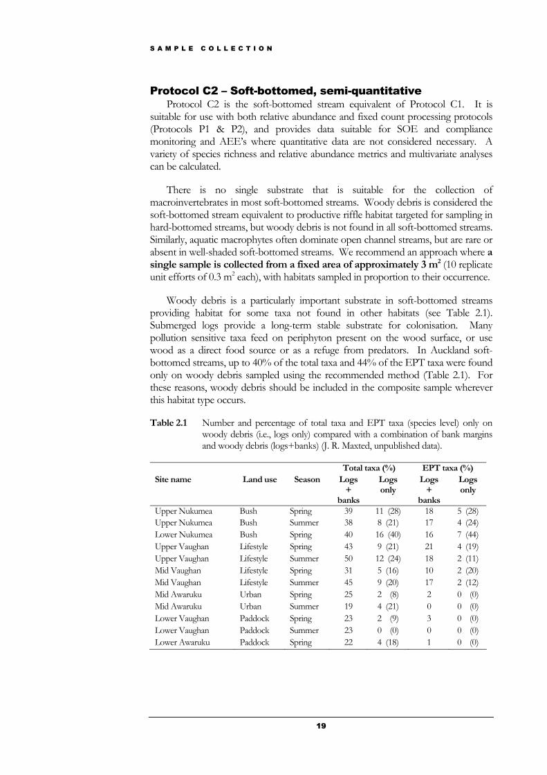
Woody debris is a particularly important substrate in soft-bottomed streams providing habitat for some taxa not found in other habitats (see Table 2.1). Submerged logs provide a long-term stable substrate for colonisation. Many pollution sensitive taxa feed on periphyton present on the wood surface, or use wood as a direct food source or as a refuge from predators. In Auckland soft-bottomed streams, up to 40% of the total taxa and 44% of the EPT taxa were found only on woody debris sampled using the recommended method (Table 2.1). For these reasons, woody debris should be included in the composite sample wherever this habitat type occurs.
Table 2.1 Number and percentage of total taxa and EPT taxa (species level) only on woody debris (i.e., logs only) compared with a combination of bank margins and woody debris (logs+banks) (J. R. Maxted, unpublished data).
Total taxa (%) EPT taxa (%) Site name Land use Season Logs
+ banks
Logs only
Logs +
banks
Logs only
Upper Nukumea Bush Spring 39 11 (28) 18 5 (28) Upper Nukumea Bush Summer 38 8 (21) 17 4 (24) Lower Nukumea Bush Spring 40 16 (40) 16 7 (44) Upper Vaughan Lifestyle Spring 43 9 (21) 21 4 (19) Upper Vaughan Lifestyle Summer 50 12 (24) 18 2 (11) Mid Vaughan Lifestyle Spring 31 5 (16) 10 2 (20) Mid Vaughan Lifestyle Summer 45 9 (20) 17 2 (12) Mid Awaruku Urban Spring 25 2 (8) 2 0 (0) Mid Awaruku Urban Summer 19 4 (21) 0 0 (0) Lower Vaughan Paddock Spring 23 2 (9) 3 0 (0) Lower Vaughan Paddock Summer 23 0 (0) 0 0 (0) Lower Awaruku Paddock Spring 22 4 (18) 1 0 (0)
S A M P L E C O L L E C T I O N
20
Sampling is undertaken while moving progressively upstream so that submerged substrates can be seen easily and are undisturbed until sampled. Hard substrates such as boulders, rock shelves, and man-made materials (e.g., concrete, gabions, shopping trolleys) are avoided or sampled separately to promote data comparability between soft-bottomed sites. The proportions of each habitat sampled should be recorded on the field sheets and final data spreadsheets to aid interpretation (e.g., 5/4/1, wood/bank margins/macrophytes).
As with Protocol C1, several sampling efforts should be pooled to create the sample for soft-bottomed streams. A single sample comprises 10 unit efforts of approximately 0.3 m2 area each (total 3 m2). Each unit effort should be transferred separately to a bucket or sieve bucket to avoid net clogging or loss of macroinvertebrates. The material collected in bank margins and macrophytes may be transferred to the bucket by banging the net over the mouth of the bucket to save time.
The following techniques should be used for different habitats to collect a unit effort of an area of approximately 0.3 m2.
Bank Margins A section of bank containing stable structure including roots and woody snags should be selected for sampling. The substrate is disturbed aggressively (i.e., jabbed) with the D-net for a distance of 1-metre followed by 2 - 3 cleaning sweeps to collect dislodged organisms. Collection is done above the bottom of the stream to avoid scraping the streambed and filling the net with fine detritus, sand, and mud. Filamentous algae should be avoided where possible. Each unit collection effort represents an area of approximately 0.3 m2.
Submerged Woody Debris Woody debris should be placed over the mouth of the bucket or sieve bucket, and water poured over the material as it is brushed by hand (this requires 2 people). Several pieces of woody debris may be placed in the bucket at once before hand-brushing separately. Brushes are not recommended because the hard bristles may damage delicate specimens and generate large amounts of detritus. Woody debris includes large branches (50 - 100 mm diameter) and small logs (200 - 300 mm diameter). The woody material should be inspected visually and any organisms removed (with the aid of forceps) before placing back into the stream. Medium to large logs (> 300 mm diameter) should be left in place, and may be sampled by hand brushing the substrate underwater while holding the net immediately downstream, provided there is sufficient velocity. Each metre of woody debris is a unit collection effort and represents an area of approximately 0.3 m2.
Aquatic Macrophytes Macrophyte beds are sampled by jabbing the net in submerged plants for a distance of approximately 1-metre to dislodge organisms, followed by 2 - 3 cleaning sweeps. Place clumps of plants that have been disturbed in the net (do not uproot) and shake and brush by hand to dislodge organisms. Sample a variety of velocity regimes and macrophyte species. Collection is done off the bottom of the stream to avoid the collection of fine detritus, sand, and mud. Filamentous algae are avoided where possible. Each unit collection effort represents an area of approximately 0.3 m2.
S A M P L E C O L L E C T I O N
21
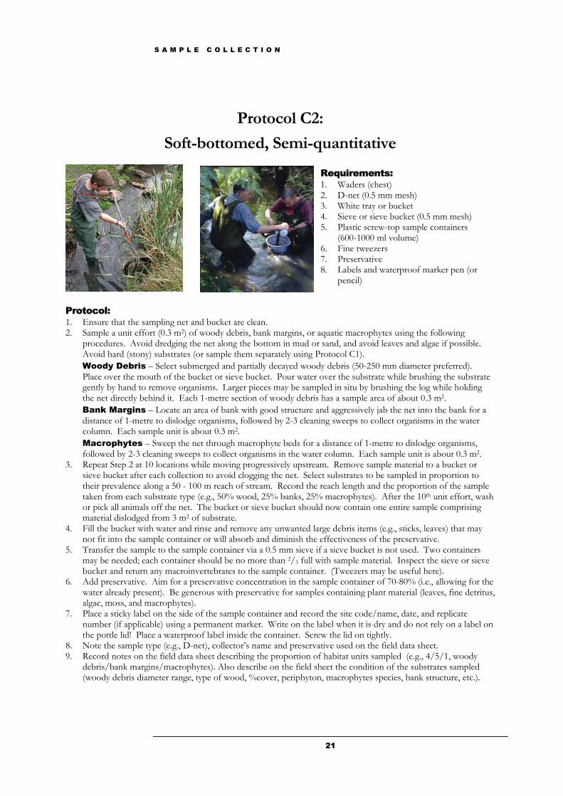
Protocol C2:
Soft-bottomed, Semi-quantitative
Requirements: 1. Waders (chest) 2. D-net (0.5 mm mesh) 3. White tray or bucket 4. Sieve or sieve bucket (0.5 mm mesh) 5. Plastic screw-top sample containers
(600-1000 ml volume) 6. Fine tweezers 7. Preservative 8. Labels and waterproof marker pen (or
pencil)
Protocol: 1. Ensure that the sampling net and bucket are clean. 2. Sample a unit effort (0.3 m2) of woody debris, bank margins, or aquatic macrophytes using the following
procedures. Avoid dredging the net along the bottom in mud or sand, and avoid leaves and algae if possible. Avoid hard (stony) substrates (or sample them separately using Protocol C1). Woody Debris – Select submerged and partially decayed woody debris (50-250 mm diameter preferred). Place over the mouth of the bucket or sieve bucket. Pour water over the substrate while brushing the substrate gently by hand to remove organisms. Larger pieces may be sampled in situ by brushing the log while holding the net directly behind it. Each 1-metre section of woody debris has a sample area of about 0.3 m2. Bank Margins – Locate an area of bank with good structure and aggressively jab the net into the bank for a distance of 1-metre to dislodge organisms, followed by 2-3 cleaning sweeps to collect organisms in the water column. Each sample unit is about 0.3 m2. Macrophytes – Sweep the net through macrophyte beds for a distance of 1-metre to dislodge organisms, followed by 2-3 cleaning sweeps to collect organisms in the water column. Each sample unit is about 0.3 m2.
3. Repeat Step 2 at 10 locations while moving progressively upstream. Remove sample material to a bucket or sieve bucket after each collection to avoid clogging the net. Select substrates to be sampled in proportion to their prevalence along a 50 - 100 m reach of stream. Record the reach length and the proportion of the sample taken from each substrate type (e.g., 50% wood, 25% banks, 25% macrophytes). After the 10th unit effort, wash or pick all animals off the net. The bucket or sieve bucket should now contain one entire sample comprising material dislodged from 3 m2 of substrate.
4. Fill the bucket with water and rinse and remove any unwanted large debris items (e.g., sticks, leaves) that may not fit into the sample container or will absorb and diminish the effectiveness of the preservative.
5. Transfer the sample to the sample container via a 0.5 mm sieve if a sieve bucket is not used. Two containers may be needed; each container should be no more than 2/3 full with sample material. Inspect the sieve or sieve bucket and return any macroinvertebrates to the sample container. (Tweezers may be useful here).
6. Add preservative. Aim for a preservative concentration in the sample container of 70-80% (i.e., allowing for the water already present). Be generous with preservative for samples containing plant material (leaves, fine detritus, algae, moss, and macrophytes).
7. Place a sticky label on the side of the sample container and record the site code/name, date, and replicate number (if applicable) using a permanent marker. Write on the label when it is dry and do not rely on a label on the pottle lid! Place a waterproof label inside the container. Screw the lid on tightly.
8. Note the sample type (e.g., D-net), collector’s name and preservative used on the field data sheet. 9. Record notes on the field data sheet describing the proportion of habitat units sampled (e.g., 4/5/1, woody
debris/bank margins/macrophytes). Also describe on the field sheet the condition of the substrates sampled (woody debris diameter range, type of wood, %cover, periphyton, macrophytes species, bank structure, etc.).
S A M P L E C O L L E C T I O N
22
Protocol C3 – Hard-bottomed, quantitative The purpose of quantitative sampling is to estimate densities (usually numbers
per square metre) of macroinvertebrates present at a sampling site. Quantitative data, being more costly to obtain, are most suited to compliance monitoring or AEEs where density effects are anticipated. Macroinvertebrate densities are highly variable, both spatially and temporally, frequently in response to flow and substrate conditions. Therefore, isolated density estimates may have limited value unless the flow history and substrate conditions are known, or unless all sampling (say upstream and downstream of a discharge) is undertaken on the same day. In our view, SOE monitoring does not normally warrant the collection of quantitative data and it is likely that densities will show flow-related variation if SOE sampling is spread over several weeks. There are no limits on the metrics and data analyses possible if quantitative data are collected.
Quantitative sampling in hard-bottomed streams can be achieved using many different techniques (see review in Merritt & Cummins 1996). Regardless of which sampling device is used in a programme, the same device should be used for all sampling. Different sampling devices may be more or less efficient for sampling some taxa so using more than one sampling method during a study may affect the consistency of the data (Winterbourn 1985). With this in mind, we recommend using a Surber sampler for all quantitative sampling in hard-bottomed streams.
The Surber sampler (Surber 1937) - a net attached to a grid frame that enables the user to collect a sample over a known area of substrate - is one of the most commonly used devices for sampling hard-bottomed stream sites both in New Zealand and overseas. While it is an indispensable apparatus for sampling stream invertebrates it does have limitations that users need to be aware of. As with many sampling devices in flowing waters, the Surber sampler relies on stream current to carry animals and detritus into the net. The assumption made when employing the Surber sampler is that, as the substrate is disturbed, organisms and detritus from within the sampling area (and not elsewhere) will all be transported downstream, and retained in the net. This assumption is only valid when certain precautions are taken:
1. Sampling must proceed in an upstream direction, with the Surber placed on an undisturbed patch of streambed. Unlike D-net sampling the operator should not stand upstream of the Surber. Likewise, sampling should not be undertaken downstream of areas where others may be working (The Surber catches drifting organisms as well as benthos).
2. Ideally, the Surber sampler should be used in water no deeper than the top of the frame (i.e., ca. 32 cm for a 0.1 m2 Surber). However, sampling can be undertaken in deeper provided that there is a good flow through the net so that backflow does not result in animals being lost around the sides and over the top of the net.
3. The Surber sampler is not effective in low velocity areas (e.g., pools or edge habitats). There must be sufficient current to carry organisms and detritus into
S A M P L E C O L L E C T I O N
23
the net, without risk of loss from backflow. If necessary, a current can be created by hand.
4. There is an obvious limit to the size of substrate that can be effectively sampled with a Surber sampler, that being the width of the frame (ca. 32 cm). Generally, the Surber sampler works best in gravel and small cobble substrates. Larger cobbles can cause the sampler to lose its seal with the bed, and the sampler can be filled with sand and silt if used in very fine sediments.
5. An effective seal must be formed between the area of streambed to be sampled and the bottom of the Surber frame, otherwise animals may be lost around the base of the sampler. Rubber skirts, foam pads, or lengths of chain can be fitted to improve the seal, but a rolled up towel can also be used. A rubber flap can also be attached beneath the mouth of the sampler to protect the net from abrasion again sharp stones.
6. Care should be taken to prevent the net becoming clogged, as this leads to backflow and loss of animals. If the net begins to balloon out and fill with water it helps to slap the side of the net, or shake it to dislodge the fine detritus that is blocking the mesh. Do not dislodge the sampling frame.
7. Except in bedrock or clay-bottomed streams, the Surber sampler is, in fact, a volume sampler rather than an area sampler. Unfortunately while the area of the sampler is fixed it is much more difficult to ensure that samples are of a uniform volume (and therefore comparable across sites/samples). The only way around this is to sample the substrate to a prescribed depth – usually 5 - 10 cm. A screwdriver with a mark on the blade can be used as a guide to show when the substrate has been disturbed to the prescribed depth. The depth of sampling should be noted.
8. In addition to sampling to a prescribed depth, the disturbance procedure should be standardised and may involve digging into the streambed with, hands (look out for broken glass!), or implements (e.g., handle of scrubbing brush, screwdriver) and brushing larger stones, with a soft-bristled brush. If stones are not scrubbed, some species that strongly adhere to the substrate will be missed. This procedure may damage soft-bodied specimens, but better a damaged specimen than no specimen at all!
9. Finally, be aware that bias can result from different personnel undertaking sampling. Never assume that your staff know what they are doing – provide them with proper instruction.
S A M P L E C O L L E C T I O N
24
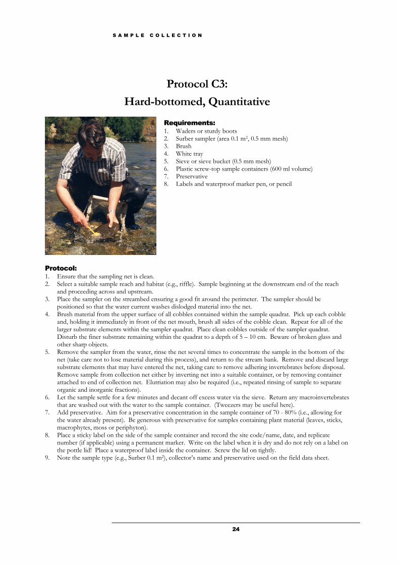
Protocol C3:
Hard-bottomed, Quantitative
Requirements: 1. Waders or sturdy boots 2. Surber sampler (area 0.1 m2, 0.5 mm mesh) 3. Brush 4. White tray 5. Sieve or sieve bucket (0.5 mm mesh) 6. Plastic screw-top sample containers (600 ml volume) 7. Preservative 8. Labels and waterproof marker pen, or pencil
Protocol: 1. Ensure that the sampling net is clean. 2. Select a suitable sample reach and habitat (e.g., riffle). Sample beginning at the downstream end of the reach
and proceeding across and upstream. 3. Place the sampler on the streambed ensuring a good fit around the perimeter. The sampler should be
positioned so that the water current washes dislodged material into the net. 4. Brush material from the upper surface of all cobbles contained within the sample quadrat. Pick up each cobble
and, holding it immediately in front of the net mouth, brush all sides of the cobble clean. Repeat for all of the larger substrate elements within the sampler quadrat. Place clean cobbles outside of the sampler quadrat. Disturb the finer substrate remaining within the quadrat to a depth of 5 – 10 cm. Beware of broken glass and other sharp objects.
5. Remove the sampler from the water, rinse the net several times to concentrate the sample in the bottom of the net (take care not to lose material during this process), and return to the stream bank. Remove and discard large substrate elements that may have entered the net, taking care to remove adhering invertebrates before disposal. Remove sample from collection net either by inverting net into a suitable container, or by removing container attached to end of collection net. Elutriation may also be required (i.e., repeated rinsing of sample to separate organic and inorganic fractions).
6. Let the sample settle for a few minutes and decant off excess water via the sieve. Return any macroinvertebrates that are washed out with the water to the sample container. (Tweezers may be useful here).
7. Add preservative. Aim for a preservative concentration in the sample container of 70 - 80% (i.e., allowing for the water already present). Be generous with preservative for samples containing plant material (leaves, sticks, macrophytes, moss or periphyton).
8. Place a sticky label on the side of the sample container and record the site code/name, date, and replicate number (if applicable) using a permanent marker. Write on the label when it is dry and do not rely on a label on the pottle lid! Place a waterproof label inside the container. Screw the lid on tightly.
9. Note the sample type (e.g., Surber 0.1 m2), collector’s name and preservative used on the field data sheet.
S A M P L E C O L L E C T I O N
25
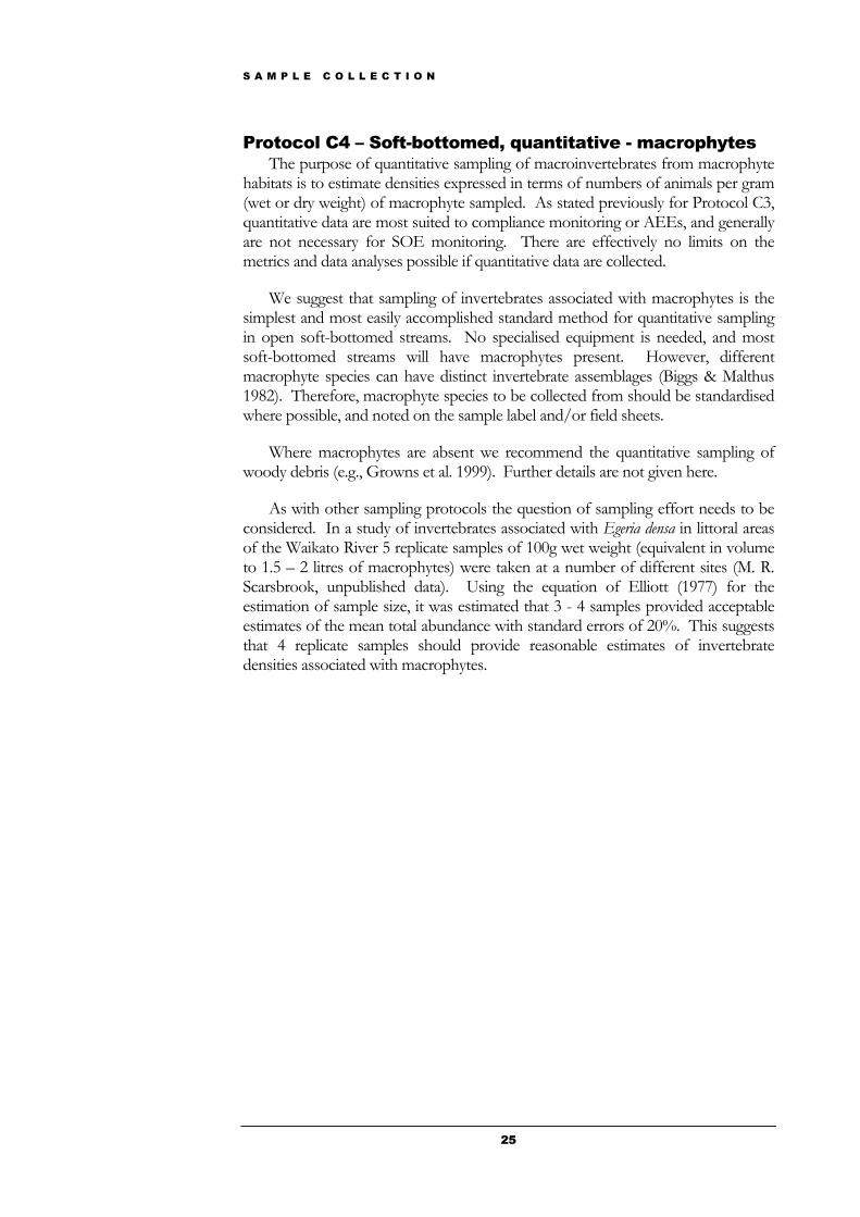
Protocol C4 – Soft-bottomed, quantitative - macrophytes The purpose of quantitative sampling of macroinvertebrates from macrophyte
habitats is to estimate densities expressed in terms of numbers of animals per gram (wet or dry weight) of macrophyte sampled. As stated previously for Protocol C3, quantitative data are most suited to compliance monitoring or AEEs, and generally are not necessary for SOE monitoring. There are effectively no limits on the metrics and data analyses possible if quantitative data are collected.
We suggest that sampling of invertebrates associated with macrophytes is the simplest and most easily accomplished standard method for quantitative sampling in open soft-bottomed streams. No specialised equipment is needed, and most soft-bottomed streams will have macrophytes present. However, different macrophyte species can have distinct invertebrate assemblages (Biggs & Malthus 1982). Therefore, macrophyte species to be collected from should be standardised where possible, and noted on the sample label and/or field sheets.
Where macrophytes are absent we recommend the quantitative sampling of woody debris (e.g., Growns et al. 1999). Further details are not given here.
As with other sampling protocols the question of sampling effort needs to be considered. In a study of invertebrates associated with Egeria densa in littoral areas of the Waikato River 5 replicate samples of 100g wet weight (equivalent in volume to 1.5 – 2 litres of macrophytes) were taken at a number of different sites (M. R. Scarsbrook, unpublished data). Using the equation of Elliott (1977) for the estimation of sample size, it was estimated that 3 - 4 samples provided acceptable estimates of the mean total abundance with standard errors of 20%. This suggests that 4 replicate samples should provide reasonable estimates of invertebrate densities associated with macrophytes.
S A M P L E C O L L E C T I O N
26
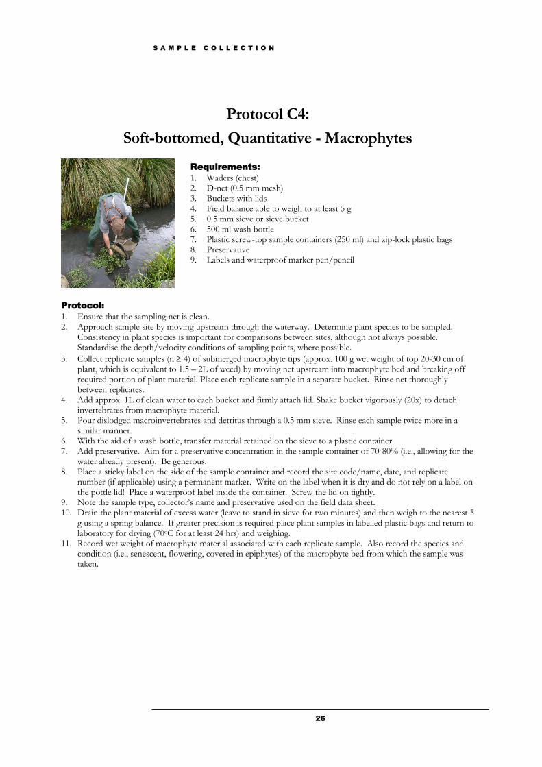
Protocol C4:
Soft-bottomed, Quantitative - Macrophytes
Requirements: 1. Waders (chest) 2. D-net (0.5 mm mesh) 3. Buckets with lids 4. Field balance able to weigh to at least 5 g 5. 0.5 mm sieve or sieve bucket 6. 500 ml wash bottle 7. Plastic screw-top sample containers (250 ml) and zip-lock plastic bags 8. Preservative 9. Labels and waterproof marker pen/pencil
Protocol: 1. Ensure that the sampling net is clean. 2. Approach sample site by moving upstream through the waterway. Determine plant species to be sampled.
Consistency in plant species is important for comparisons between sites, although not always possible. Standardise the depth/velocity conditions of sampling points, where possible.
3. Collect replicate samples (n ≥ 4) of submerged macrophyte tips (approx. 100 g wet weight of top 20-30 cm of plant, which is equivalent to 1.5 – 2L of weed) by moving net upstream into macrophyte bed and breaking off required portion of plant material. Place each replicate sample in a separate bucket. Rinse net thoroughly between replicates.
4. Add approx. 1L of clean water to each bucket and firmly attach lid. Shake bucket vigorously (20x) to detach invertebrates from macrophyte material.
5. Pour dislodged macroinvertebrates and detritus through a 0.5 mm sieve. Rinse each sample twice more in a similar manner.
6. With the aid of a wash bottle, transfer material retained on the sieve to a plastic container. 7. Add preservative. Aim for a preservative concentration in the sample container of 70-80% (i.e., allowing for the
water already present). Be generous. 8. Place a sticky label on the side of the sample container and record the site code/name, date, and replicate
number (if applicable) using a permanent marker. Write on the label when it is dry and do not rely on a label on the pottle lid! Place a waterproof label inside the container. Screw the lid on tightly.
9. Note the sample type, collector’s name and preservative used on the field data sheet. 10. Drain the plant material of excess water (leave to stand in sieve for two minutes) and then weigh to the nearest 5
g using a spring balance. If greater precision is required place plant samples in labelled plastic bags and return to laboratory for drying (70oC for at least 24 hrs) and weighing.
11. Record wet weight of macrophyte material associated with each replicate sample. Also record the species and condition (i.e., senescent, flowering, covered in epiphytes) of the macrophyte bed from which the sample was taken.
S A M P L E C O L L E C T I O N
27
Quality Control (QC) Quality control of field sample collection is difficult. To our knowledge there
are no robust QC procedures for field sampling. However, most international and national monitoring programmes have instigated extensive training programmes to improve the consistency of sample collection. Periodic training in the use of the protocols for sample collection is recommended. In the first instance, within any organisation, more experienced personnel should provide appropriate instruction and supervision to new staff. Ideally, however, an appropriate agency or professional body (e.g., NZ Limnological Society) should provide training.
We recommend a minimum field crew of two people for efficiency and safety (although this may not be necessary when sampling small streams). At least one person in the crew should be fully trained in the collection methods. Checking of sample collection techniques between investigators within and between organisations (e.g., Regional Councils, Territorial Local Authorities, consultants) should be done periodically to improve consistency.
Sample Labelling All samples collected should be clearly labelled. We recommend a sticky label
on the side of the sample container with information written using a permanent marker (i.e., waterproof and alcohol resistant felt pen or pencil). Reliance solely on labels on pottle lids is not recommended – lids can easily be interchanged. A label written in pencil on waterproof paper should also be placed inside the container.
The information required on sample labels must be sufficient to ensure that each sample has a unique identity. Normally this would include:-
Site location (e.g., Patea River @ Skinner Rd)
Sampling date: (e.g., 29 August 2001)
Sample code: We suggest numbers (or names) for site codes and letters (a, b, c, etc.) for replicates e.g., Site 1(a).
Additional information may be recorded on the sample label and/or on the field data sheet. This might include the sample type (e.g., D-net or Surber), mesh size, area sampled, collector’s name/initials, site code, NZMS260 series map reference, GPS location, or a job or project code number. Whoever has to process the samples will need to know what sample processing protocol to use.
Patea River @ Skinner Rd PAT000360
HN (a) 29 August 2001
JDS
S A M P L E P R O C E S S I N G
28
Sample Processing
Introduction hree methods of sample processing are recommended. The first method (Protocol P1) is a semi-quantitative method that provides coded abundance data on the 5-point scale developed by Stark (1998).
The second sample processing method (Protocol P2) is a 200-animal fixed count method, that follows closely the protocols outlined by the USEPA in a recent revision of Rapid Bioassessment Protocols (RBPs) (Barbour et al. 1999). The fixed count method is a widely used sub-sampling technique both in NZ and overseas.
The third method (Protocol P3) is a full count, quantitative method, which is appropriate for intensive impact assessments, especially where an anticipated impact is a change in macroinvertebrate densities. A subsampling option is provided for samples containing very high numbers of the dominant taxa. QC procedures are provided for each protocol.
Protocols P1 (coded-abundance) or P2 (200 fixed count) should meet the needs of Regional Councils for SOE monitoring, which rarely warrants quantitative data, and in most cases for compliance monitoring and environmental effects assessments too. Investigations where changes in densities may be expected (e.g., assessing the impact of nutrient discharges) may warrant the additional cost of quantitative sampling (Protocol P3).
The choice of sample processing method will dictate the range of metrics or indices that can be calculated from the resulting data. It is the responsibility of the investigator to ensure that the sample-processing methods selected will provide information that meets the requirements of the study, e.g., richness indices are highly dependent upon sampling effort and are unlikely to be comparable if different sampling methods have been used.
Chapter
3 T
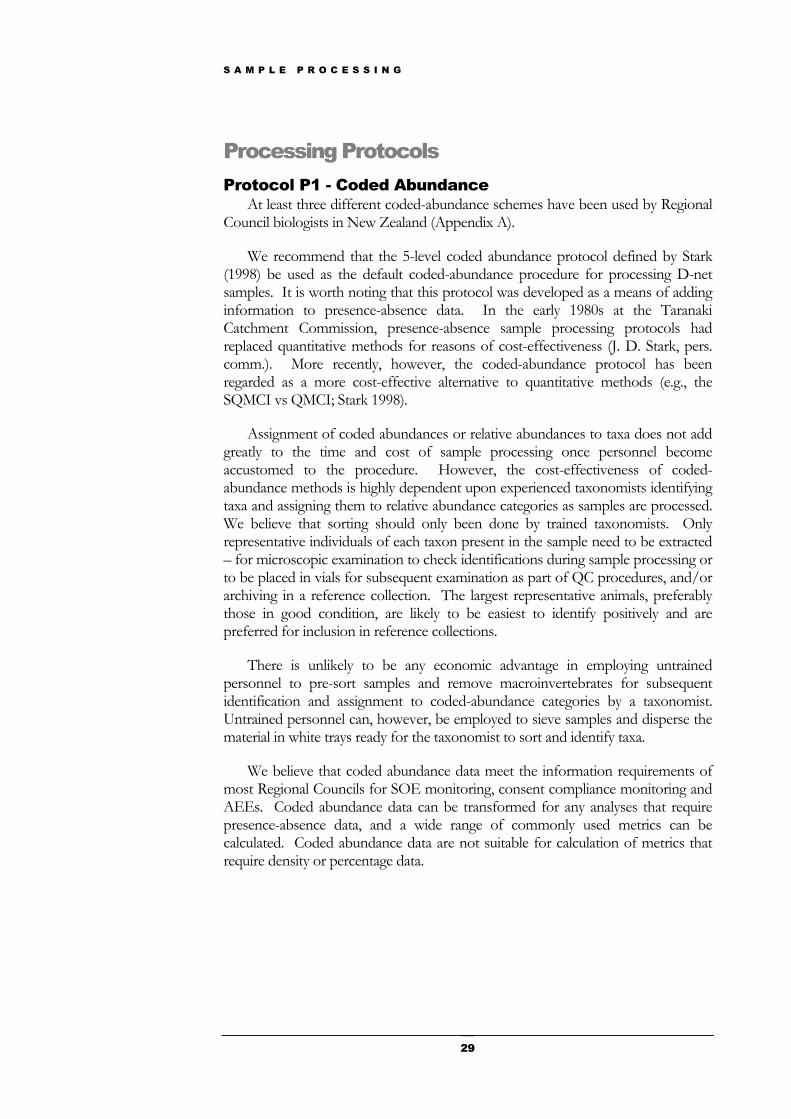
S A M P L E P R O C E S S I N G
29
Processing Protocols Protocol P1 - Coded Abundance
At least three different coded-abundance schemes have been used by Regional Council biologists in New Zealand (Appendix A).
We recommend that the 5-level coded abundance protocol defined by Stark (1998) be used as the default coded-abundance procedure for processing D-net samples. It is worth noting that this protocol was developed as a means of adding information to presence-absence data. In the early 1980s at the Taranaki Catchment Commission, presence-absence sample processing protocols had replaced quantitative methods for reasons of cost-effectiveness (J. D. Stark, pers. comm.). More recently, however, the coded-abundance protocol has been regarded as a more cost-effective alternative to quantitative methods (e.g., the SQMCI vs QMCI; Stark 1998).
Assignment of coded abundances or relative abundances to taxa does not add greatly to the time and cost of sample processing once personnel become accustomed to the procedure. However, the cost-effectiveness of coded-abundance methods is highly dependent upon experienced taxonomists identifying taxa and assigning them to relative abundance categories as samples are processed. We believe that sorting should only been done by trained taxonomists. Only representative individuals of each taxon present in the sample need to be extracted – for microscopic examination to check identifications during sample processing or to be placed in vials for subsequent examination as part of QC procedures, and/or archiving in a reference collection. The largest representative animals, preferably those in good condition, are likely to be easiest to identify positively and are preferred for inclusion in reference collections.
There is unlikely to be any economic advantage in employing untrained personnel to pre-sort samples and remove macroinvertebrates for subsequent identification and assignment to coded-abundance categories by a taxonomist. Untrained personnel can, however, be employed to sieve samples and disperse the material in white trays ready for the taxonomist to sort and identify taxa.
We believe that coded abundance data meet the information requirements of most Regional Councils for SOE monitoring, consent compliance monitoring and AEEs. Coded abundance data can be transformed for any analyses that require presence-absence data, and a wide range of commonly used metrics can be calculated. Coded abundance data are not suitable for calculation of metrics that require density or percentage data.
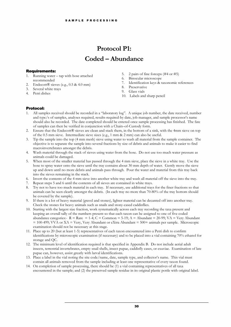
S A M P L E P R O C E S S I N G
30
Protocol P1:
Coded – Abundance
Requirements: 1. Running water – tap with hose attached
recommended 2. Endecott® sieves (e.g., 0.5 & 4.0 mm) 3. Several white trays 4. Petri dishes
5. 2 pairs of fine forceps (#4 or #5) 6. Binocular microscope 7. Identification keys & taxonomic references 8. Preservative 9. Glass vials 10. Labels and sharp pencil
Protocol: 1. All samples received should be recorded in a “laboratory log”. A unique job number, the date received, number
and type/s of samples, analyses required, results-required-by date, job manager, and sample processor’s name should also be recorded. The date completed should be entered once sample processing has finished. The fate of samples can then be verified in conjunction with a Chain–of-Custody form.
2. Ensure that the Endecott® sieves are clean and stack them, in the bottom of a sink, with the 4mm sieve on top of the 0.5 mm sieve. Intermediate sieve sizes (e.g., 1 mm & 2 mm) can also be useful.
3. Tip the sample into the top (4 mm mesh) sieve using water to wash all material from the sample container. The objective is to separate the sample into several fractions by size of debris and animals to make it easier to find macroinvertebrates amongst the debris.
4. Wash material through the stack of sieves using water from the hose. Do not use too much water pressure as animals could be damaged.
5. When most of the smaller material has passed through the 4 mm sieve, place the sieve in a white tray. Use the hose to spray water onto the sieve until the tray contains about 30 mm depth of water. Gently move the sieve up and down until no more debris and animals pass through. Pour the water and material from this tray back into the sieves remaining in the stack.
6. Invert the contents of the 4 mm sieve into another white tray and wash all material off the sieve into the tray. 7. Repeat steps 5 and 6 until the contents of all sieves are contained in white trays. 8. Try not to have too much material in each tray. If necessary, use additional trays for the finer fractions so that
animals can be seen clearly amongst the debris. (In each tray no more than 70-80% of the tray bottom should be covered by the sample).
9. If there is a lot of heavy material (gravel and stones), lighter material can be decanted off into another tray. Check the stones for heavy animals such as snails and stony-cased caddisflies.
10. Starting with the largest size fraction, work systematically across each tray recording the taxa present and keeping an overall tally of the numbers present so that each taxon can be assigned to one of five coded abundance categories:- R = Rare = 1-4; C = Common = 5-19; A = Abundant = 20-99; VA = Very Abundant = 100-499; VVA or XA = Very, Very Abundant or eXtra Abundant = 500+ animals per sample. Microscopic examination should not be necessary at this stage.
11. Place up to 20 (but at least 1-5) representatives of each taxon encountered into a Petri dish to confirm identifications by microscopic examination (if necessary) and to be placed into a vial containing 70% ethanol for storage and QC.
12. The minimum level of identification required is that specified in Appendix B. Do not include aerial adult insects, terrestrial invertebrates, empty snail shells, insect pupae, caddisfly cases, or exuviae. Examination of late pupae can, however, assist greatly with larval identifications.
13. Place a label in the vial noting the site code/name, date, sample type, and collector’s name. This vial must contain all animals removed from the sample including at least one representative of every taxon found.
14. On completion of sample processing, there should be (1) a vial containing representatives of all taxa encountered in the sample; and (2) the preserved sample residue in its original plastic pottle with original label.
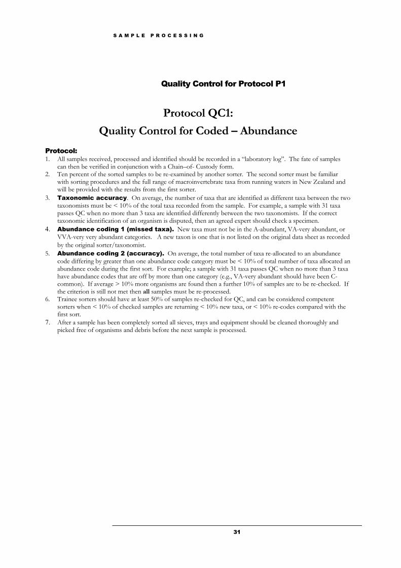
S A M P L E P R O C E S S I N G
31
Quality Control for Protocol P1
Protocol QC1:
Quality Control for Coded – Abundance
Protocol: 1. All samples received, processed and identified should be recorded in a “laboratory log”. The fate of samples
can then be verified in conjunction with a Chain–of- Custody form. 2. Ten percent of the sorted samples to be re-examined by another sorter. The second sorter must be familiar
with sorting procedures and the full range of macroinvertebrate taxa from running waters in New Zealand and will be provided with the results from the first sorter.
3. Taxonomic accuracy. On average, the number of taxa that are identified as different taxa between the two taxonomists must be < 10% of the total taxa recorded from the sample. For example, a sample with 31 taxa passes QC when no more than 3 taxa are identified differently between the two taxonomists. If the correct taxonomic identification of an organism is disputed, then an agreed expert should check a specimen.
4. Abundance coding 1 (missed taxa). New taxa must not be in the A-abundant, VA-very abundant, or VVA-very very abundant categories. A new taxon is one that is not listed on the original data sheet as recorded by the original sorter/taxonomist.
5. Abundance coding 2 (accuracy). On average, the total number of taxa re-allocated to an abundance code differing by greater than one abundance code category must be < 10% of total number of taxa allocated an abundance code during the first sort. For example; a sample with 31 taxa passes QC when no more than 3 taxa have abundance codes that are off by more than one category (e.g., VA-very abundant should have been C-common). If average > 10% more organisms are found then a further 10% of samples are to be re-checked. If the criterion is still not met then all samples must be re-processed.
6. Trainee sorters should have at least 50% of samples re-checked for QC, and can be considered competent sorters when < 10% of checked samples are returning < 10% new taxa, or < 10% re-codes compared with the first sort.
7. After a sample has been completely sorted all sieves, trays and equipment should be cleaned thoroughly and picked free of organisms and debris before the next sample is processed.
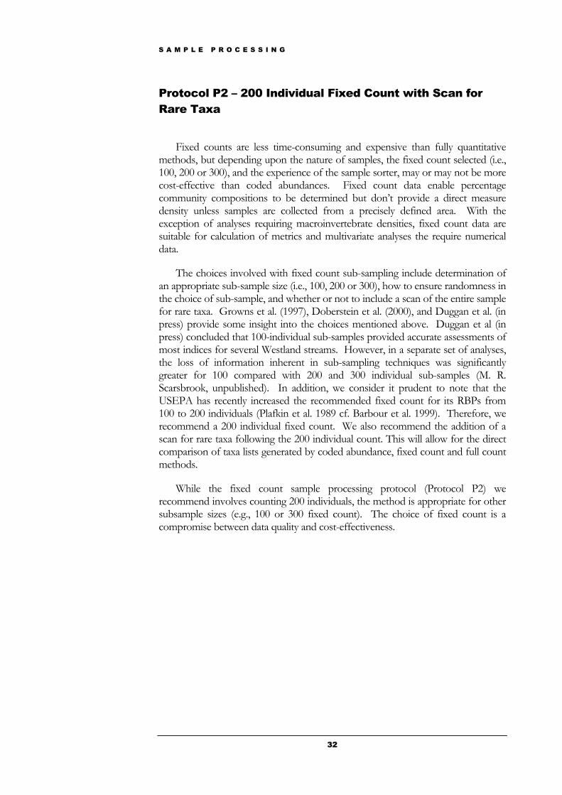
S A M P L E P R O C E S S I N G
32
Protocol P2 – 200 Individual Fixed Count with Scan for Rare Taxa
Fixed counts are less time-consuming and expensive than fully quantitative methods, but depending upon the nature of samples, the fixed count selected (i.e., 100, 200 or 300), and the experience of the sample sorter, may or may not be more cost-effective than coded abundances. Fixed count data enable percentage community compositions to be determined but don’t provide a direct measure density unless samples are collected from a precisely defined area. With the exception of analyses requiring macroinvertebrate densities, fixed count data are suitable for calculation of metrics and multivariate analyses the require numerical data.
The choices involved with fixed count sub-sampling include determination of an appropriate sub-sample size (i.e., 100, 200 or 300), how to ensure randomness in the choice of sub-sample, and whether or not to include a scan of the entire sample for rare taxa. Growns et al. (1997), Doberstein et al. (2000), and Duggan et al. (in press) provide some insight into the choices mentioned above. Duggan et al (in press) concluded that 100-individual sub-samples provided accurate assessments of most indices for several Westland streams. However, in a separate set of analyses, the loss of information inherent in sub-sampling techniques was significantly greater for 100 compared with 200 and 300 individual sub-samples (M. R. Scarsbrook, unpublished). In addition, we consider it prudent to note that the USEPA has recently increased the recommended fixed count for its RBPs from 100 to 200 individuals (Plafkin et al. 1989 cf. Barbour et al. 1999). Therefore, we recommend a 200 individual fixed count. We also recommend the addition of a scan for rare taxa following the 200 individual count. This will allow for the direct comparison of taxa lists generated by coded abundance, fixed count and full count methods.
While the fixed count sample processing protocol (Protocol P2) we recommend involves counting 200 individuals, the method is appropriate for other subsample sizes (e.g., 100 or 300 fixed count). The choice of fixed count is a compromise between data quality and cost-effectiveness.
S A M P L E P R O C E S S I N G
33
Protocol P2:
200 Fixed Count + Scan for Rare Taxa
Requirements: 1. Running water – tap with hose recommended 2. 0.5 mm sieve 3. Clean, flat-bottomed, white tray marked in 6 cm
x 6 cm grids 4. 6 cm x 6 cm cookie cutters 5. Fine forceps 6. 70% ethanol preservative
7. Specimen vials with stoppers 8. Bench lamp 9. Labels and sharp pencil 10. Counter 11. 500 ml wash bottle 12. Identification keys & taxonomic references 13. Binocular dissecting microscope and light source
for species identification Protocol: 1. All samples received should be recorded in a “laboratory log”. A unique job number, the date received, number
and type/s of samples, analyses required, results-required-by date, job manager, and sample processor’s name should be recorded. The date completed should be entered once sample processing has finished. The fate of samples can be verified in conjunction with a Chain–of-Custody form.
2. Thoroughly rinse sample in a clean 0.5 mm sieve to remove preservative and fine sediment. Large organic material (whole leaves, twigs, algal or macrophyte mats, etc.) not removed in the field should be rinsed, visually inspected for organisms, and discarded. Gently mix the sample by hand while rinsing, and continue until wash water runs clear and the sample is thoroughly homogenised (i.e., break down lumps of algae etc). A coarse sieve (e.g., 4 mm) can be helpful for removing larger pieces of unwanted organic material so long as all macroinvertebrates are picked out and placed into the 0.5 mm sieve.
3. After washing, transfer contents of sieve to a white sorting tray marked with grids approximately 6 cm x 6 cm (use black indelible marker). Visually check sieve before washing in preparation for next sample. Using the wash bottle spread the sample evenly across the tray. There should be enough water to just cover all material. If the samples have been preserved in alcohol some organisms (particularly ostracods and early instar insects) may float on the surface. If this is occurs add a drop of washing detergent and stir gently.
4. Use a random numbers table to select a starting grid square within the tray. A cookie cutter (6 x 6 cm) is recommended to delineate the chosen grid square. Moving systematically across the square remove all organisms visible to the naked eye. Place captured organisms in a separate labelled vial (add preservative), counting each individual with a counter. When complete, do a final check of the square’s contents to ensure no animals have been missed.
5. Any organism that is lying over a line separating two grids is considered to be in the square containing its head. In those instances where it may not be possible to determine the location of the head (worms for instance), the organism is considered to be in the square containing most of its body.
6. After all visible organisms have been removed use forceps and/or a suction device to transfer remaining detritus to a container labelled as “sorted residue”. Include location and date information (as per original sample label). Add preservative. This provides material for sorting QA/QC procedures.
7. If a total of at least 200 organisms have been obtained sample sorting ceases. However, if less than 200 organisms have been enumerated, place another cookie cutter on a second randomly chosen square. Continue this process until at least 200 animals have been captured.
8. Once a square has been started it should be finished, even if the 200 individual total is exceeded. The total number of grid squares covered should be noted, along with the total individual count.
9. Save the remaining unsorted sample debris residue in a separate container labelled "sample residue"; this container should include the original sample label. Add preservative.
10. The “sample residue” and vial containing the 200 individuals must be sorted by an experience taxonomist. (Note: In situations where the sorter is an experienced taxonomist, invertebrate identification and counting can be carried out during the sorting process to save time). Pour the 200 individual sample into a Petri-dish or Bogorov tray and observe under a binocular microscope. Compile a taxa list and count the numbers of each taxon. Return the 200 individuals to a labelled vial and add preservative. This sample will be used for taxonomic QA/QC (see below).
S A M P L E P R O C E S S I N G
34
11. The minimum level of identification required is that specified in Appendix B. Do not include aerial adult
insects, pupae, terrestrial invertebrates, empty snail shells, caddisfly cases or exuviae. Examination of late pupae can, however, assist greatly with larval identifications.
12. Complete the taxa list by scanning the “sample residue” for rare taxa. This is carried out with the sample spread in white sorting trays. Any rare taxa obtained should be placed in a labelled vial with preservative. This is also an opportunity to remove larger (e.g., late instar) or better-conditioned individuals of taxa already encountered to assist in identification.
13. The vial containing the 200 individuals, and the vial containing rare taxa should be taped together. Record the taxa found in the scan for rare taxa separately from the 200 fixed count data.
14. Return the “sample residue” to its container with the original labels. 15. On completion of sample processing there should be: (1) A labelled container holding the sample residue
(already scanned for rare taxa); (2) A labelled container holding the sorted residue (required for QC procedures to assess sorting efficiency); (3) A labelled vial containing the 200+ individuals; and (4) A labelled vial containing the rare taxa (not included in the 200+ sample) removed from the sample residue.
Quality Control for Protocol P2
Protocol QC2:
Quality Control for Fixed Count
Protocol: 1. All samples received, processed and identified should be recorded in a “laboratory log”. The fate of samples
can then be verified in conjunction with a Chain–of- Custody form. 2. Ten percent of the sorted samples to be re-examined by another sorter. The second sorter must be familiar
with sorting procedures and the full range of macroinvertebrate taxa from running waters in New Zealand and will be provided with the results from the first sorter.
3. The fixed count protocol requires examination of the sample residue (were all rare taxa removed by the first sorter?) and the sorted residue (were any animals missed during the collection of the 200+ individual sub-sample?). A check on the taxonomic efficiency of both the 200+ sub-sample and the vial of rare taxa are also required.
4. Taxonomic accuracy. On average, the number of taxa that are identified as different taxa, in either the full 200+ individual vial, or the rare taxa vial, between the two taxonomists must be < 10% of the total taxa recorded from the sample. For example, a sample with 31 taxa passes QC when no more than 3 taxa are identified differently between the two taxonomists. If the correct taxonomic identification of an organism is disputed, then a specimen should be checked by an agreed expert.
5. Sorting accuracy 1 (missed taxa). If average > 10% new species are found in the sample residue then the scan for rare taxa is deemed to have failed and a further 10% of samples are to be re-checked. If the criterion is still not met then all samples must be re-processed.
6. Sorting accuracy 2 (missed individuals). If average > 10% more organisms are found in the sorted residue then a further 10% of samples are to be re-checked. If the criterion is still not met then all samples must be re-processed.
7. Trainee sorters should have at least 50% of samples re-checked for QC, and can be considered competent sorters when < 10% of checked samples are returning < 10% new taxa, or < 10% re-codes than first sort.
8. After a sample has been completely sorted all sieves, trays and equipment should be thoroughly cleaned and picked free of organisms and debris before the next sample is begun.
S A M P L E P R O C E S S I N G
35
Protocol P3 - Full Count with Subsampling Option Full counts are more time-consuming and expensive than coded abundance or
fixed count methods, and are not always necessary to meet SOE, AEE, and compliance monitoring objectives. They provide a direct measure of abundance (and percentage composition), and are necessary when direct, statistical comparisons of abundance or calculation of metrics requiring numerical data are desired. Assuming adequate replication, there are effectively no limitations on subsequent data analyses if all animals in samples are counted.
The full count sorting procedure is similar to Protocol P1 except that all of the organisms are removed from the sample, and the samples normally have been collected using a quantitative sampler (e.g., Surber sampler) rather than a D-net, or comprise a known weight of macrophyte. Quality control is achieved by checking the sorted detritus to ensure that target organisms have been removed. A fixed-fraction subsampling option is presented for the fixed-fraction subsampling of very abundant taxa (> 500 individuals) to save time.
S A M P L E P R O C E S S I N G
36
Protocol P3:
Full Count with Subsampling Option Requirements: 1. Running water tap and sink 2. Endecott® sieves (0.5, 1.0, 2.0, & 4.0 mm) 3. Grided white trays 4. Petri dishes 5. 2 pairs of fine forceps (#4 or #5)
6. Binocular microscope 7. Identification keys & taxonomic references 8. 70% ethanol preservative 9. Glass vials and/or pottles 10. Labels and sharp pencil
Protocol: 1. Sieve and place the sample in grided sorting trays following Protocol P1. 2. Starting with the largest size fraction, work systematically across each tray removing all of the organisms in the
sample. Normal eyesight should be precise enough to detect organisms > 1mm in total length. Do not use magnification.
3. Place the organisms of each taxon encountered into separate Petri dish to confirm identifications by microscopic examination (if necessary). Place sorted animals into vials or pottles containing 70% alcohol for storage and QC.
4. The minimum level of identification required is that specified in Appendix B. Do not include aerial adult insects, pupae, terrestrial invertebrates, empty snail shells, caddisfly cases or exuviae. . Examination of late pupae can, however, assist greatly with larval identifications.
5. Place a label in the vial or pottle noting the site code/name, date, sample type, and collector’s name. Label multiple containers (e.g., “1 of 2, 2 of 2).
6. On completion of sample processing, there should be (1) labelled vials or pottles containing sorted organisms, and (2) the preserved sample residue in its original plastic pottle with the original label.
Subsampling Option: (Note: Only very abundant taxa should be subsampled. Full counts should be made for all other taxa). 1. Subsampling of very abundant taxa (> 500 individuals) can save considerable time. 2. Count the number individuals of each very abundant taxon from a fixed fraction (between 10% and 50%
recommended) of the sample grids for each sorting tray. Estimate the total abundance for that taxon by multiplying the number counted by between 10 (for 10% fraction) and 2 (for 50% fraction) according to the fraction of the sample that was counted.
3. Record the count estimate on the bench data sheet and note that the value is a subsampling estimate (e.g., 25% fraction).
4. Remove 10-20 representatives of each taxon subsampled and store in a separate vial or pottle from that containing the other sorted organisms.
S A M P L E P R O C E S S I N G
37
Quality Control for Protocol P3
Protocol QC3:
Quality Control for Full Count with Subsampling Option
Protocol: 1. All samples received, processed and identified should be recorded in a “laboratory log”. The fate of samples
can then be verified in conjunction with a Chain–of- Custody form. 2. Ten percent of the sorted samples to be re-examined by another sorter. The second sorter must be familiar
with sorting procedures and the full range of macroinvertebrate taxa from running waters in New Zealand and will be provided with the results from the first sorter.
3. Taxonomic accuracy. On average, the number of taxa that are identified as different taxa between the two taxonomists must be < 10% of the total taxa recorded from the sample. For example, a sample with 31 taxa passes QC when no more than 3 taxa are identified differently between the two taxonomists.
4. Sorting accuracy. On average, the total number of each taxon found in the remnant sample must be < 10% of total for each taxon counted during the first sort. If the QC sorter finds less than an average 10% more organisms than recorded in first sort then the sample passes QC requirements. If average > 10% more organisms are found then a further 10% of samples to be re-checked. If the criterion is still not met than all samples must be re-processed and resorted. If the correct taxonomic identification of an organism is disputed, then a specimen should be checked by an agreed expert.
5. Trainee sorters should have at least 50% of samples re-checked for QC, and can be considered competent sorters when < 10% of checked samples are returning < 10% more organisms and < 10% new taxa than first sort.
6. After a sample has been completely sorted all sieves, trays and equipment should be thoroughly cleaned and picked free of organisms and debris before the next sample is introduced.
S A M P L E P R O C E S S I N G
38
Taxonomic Identification Taxonomic Resolution
One of the most contentious issues in biomonitoring has been the level (from phylum to species) or taxonomic resolution to which macroinvertebrates should be identified (Bailey et al. 2001). The importance of monitoring individual species (or identification to the “lowest practical level”) was emphasised over 25 years ago when it was argued that the power to detect changes due to perturbation diminished at higher taxonomic levels because closely related species could differ substantially in their pollution tolerances and habitat preferences (Resh & Unzicker 1975; Cranston 1990). In a recent review, Lenat & Resh (2001) concluded that biological monitoring studies yield the greatest benefits using genus- or species-level taxonomy. Others have claimed that identification of macroinvertebrates to the family level (or even higher) provides sufficient resolution for accurate and sensitive bioassessment (Bowman & Bailey 1998, Wright-Stow 2001).
Bowman & Bailey (1998) examined the influence of taxonomic resolution on multivariate description of the structure of benthic macroinvertebrate communities based upon data from published studies (mainly North America, but also Australia and Yemen). They concluded that “genus-level identification did not usually provide a strikingly different description of community patterns than higher levels (e.g., family, order) of taxonomic identification.” In an investigation of 230 Canterbury streams, Wright-Stow (2001) found that metrics based on ordinal taxonomic identification (e.g., Order, Class, and Phylum) provided similar conclusions to those based on indices calculated from genus-level identifications. Hewlett (2000) found that species-level identification appeared to be unnecessary for broad-scale monitoring in Victoria, Australia, and that family-level identification could reduce the time and effort required.
We recommend the minimum level of identification is that given by Stark (1998) (Appendix B), since this level of identification is already in widespread use in New Zealand, and the utility of higher taxonomic levels has not been validated nationally. Identification of aquatic insects should use the keys provided by Winterbourn et al. (2000) and references cited therein. Molluscs should be identified using the key of Winterbourn (1973), but readers should be aware of recent changes in nomenclature. Chapman & Lewis (1976) is still the best general resource for identification of Crustacea, although it is in need of updating. Identification of other groups is at a very broad taxonomic level (e.g., Platyhelminthes, Oligochaeta), and a general invertebrate Zoology text is recommended for reference material.
If time, budget or expertise permit, identification to species is encouraged because it will provide information that will lead to a greater understanding of the pollution tolerances and habitat requirements of macroinvertebrate species. This, in turn, could lead to improvements in biotic indices and to more defensible biomonitoring programmes.
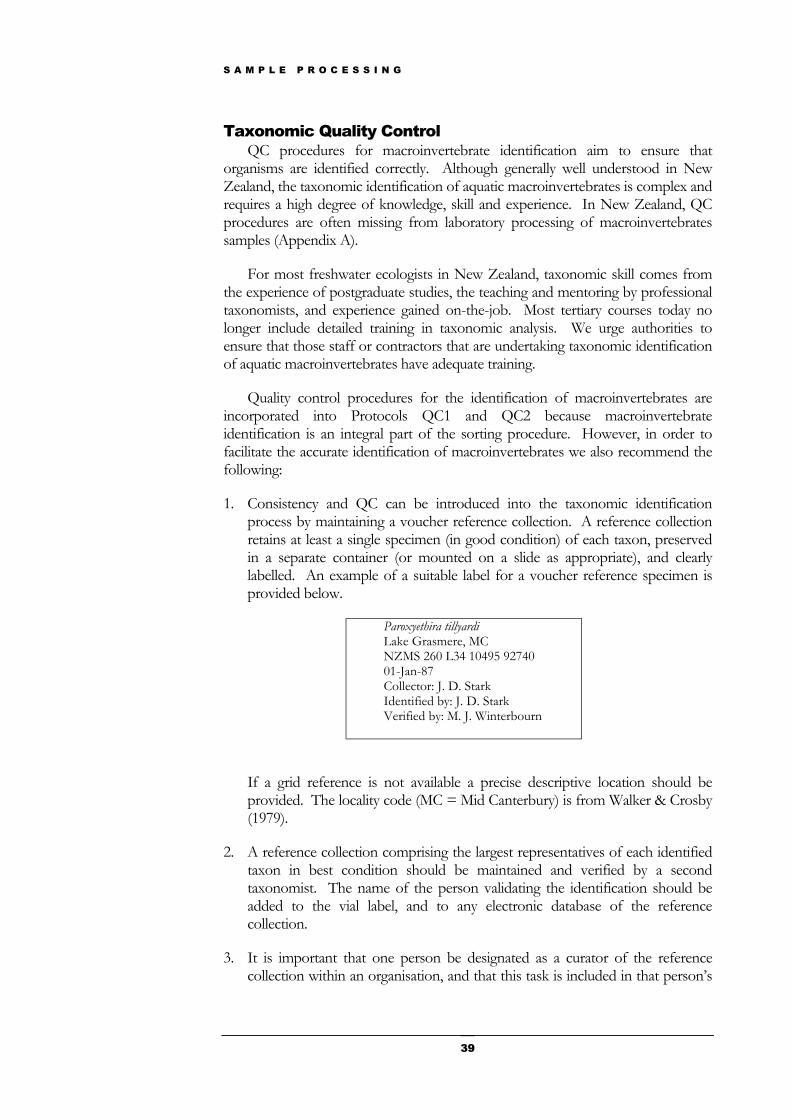
S A M P L E P R O C E S S I N G
39
Taxonomic Quality Control QC procedures for macroinvertebrate identification aim to ensure that
organisms are identified correctly. Although generally well understood in New Zealand, the taxonomic identification of aquatic macroinvertebrates is complex and requires a high degree of knowledge, skill and experience. In New Zealand, QC procedures are often missing from laboratory processing of macroinvertebrates samples (Appendix A).
For most freshwater ecologists in New Zealand, taxonomic skill comes from the experience of postgraduate studies, the teaching and mentoring by professional taxonomists, and experience gained on-the-job. Most tertiary courses today no longer include detailed training in taxonomic analysis. We urge authorities to ensure that those staff or contractors that are undertaking taxonomic identification of aquatic macroinvertebrates have adequate training.
Quality control procedures for the identification of macroinvertebrates are incorporated into Protocols QC1 and QC2 because macroinvertebrate identification is an integral part of the sorting procedure. However, in order to facilitate the accurate identification of macroinvertebrates we also recommend the following:
1. Consistency and QC can be introduced into the taxonomic identification process by maintaining a voucher reference collection. A reference collection retains at least a single specimen (in good condition) of each taxon, preserved in a separate container (or mounted on a slide as appropriate), and clearly labelled. An example of a suitable label for a voucher reference specimen is provided below.
Paroxyethira tillyardi Lake Grasmere, MC NZMS 260 L34 10495 92740 01-Jan-87 Collector: J. D. Stark Identified by: J. D. Stark Verified by: M. J. Winterbourn
If a grid reference is not available a precise descriptive location should be provided. The locality code (MC = Mid Canterbury) is from Walker & Crosby (1979).
2. A reference collection comprising the largest representatives of each identified taxon in best condition should be maintained and verified by a second taxonomist. The name of the person validating the identification should be added to the vial label, and to any electronic database of the reference collection.
3. It is important that one person be designated as a curator of the reference collection within an organisation, and that this task is included in that person’s
S A M P L E P R O C E S S I N G
40
job description. Otherwise the long-term needs of the collection can be overlooked. Every six months the entire collection should be checked to ensure levels of preservative are appropriate, and seals on vials have not perished.
4. Information on samples completed (through the identification process) will be recorded in the "sample log" notebook to track the progress of each sample within the sample lot. Tracking of each sample will be updated as each step is completed (i.e., subsampling and sorting, mounting of midges and worms, taxonomy).
Sample Storage In most cases either entire samples or “representative” samples should be kept
in long-term storage. Retaining representative samples will enable data to be re-checked at a later date. Samples should be kept at least until data from the project have been analysed and produced in a publication. Reference collections are an important part of the on-going quality control of macroinvertebrate data. These collections also form a valuable staff training resource.
Samples can usually be stored for long periods in 70% ethanol, however animals will loose their colour over time, and unless storage vials have very good seals the ethanol will evaporate slowly requiring samples to be topped up every 6-12 months. A small amount of glycerol may be added to assist long-term preservation. The collection curator should check the entire collection every six months to ensure levels of preservative are appropriate, and seals on vials have not perished.
Waterproof paper and pencil should be used for the labelling of samples for long-term storage. Waterproof paper is available from most paper suppliers. Laser printing is not permanent, and should not be used.
C O N C L U D I N G R E M A R K S
41
Concluding Remarks o there we have it. For the first time in New Zealand, clearly documented methodologies for sampling and processing aquatic macroinvertebrates from a range of habitats in wadeable streams. For the first time, a general acceptance amongst practitioners that standard methods could enhance the
value of macroinvertebrate biomonitoring as a source of information for decision-makers. For the first time, the potential to compare macroinvertebrate data from around New Zealand, and to report on the state of New Zealand’s freshwater environment (wadeable streams) using consistent aquatic macroinvertebrate data.
The opportunity for change now lies with you, the practicing biologist. Changing established patterns and routines is never easy. The thought of modifying methods and learning new ways of doing things, perhaps not even agreeing with everything that is promoted in these protocols, could be viewed as reasons for ignoring them. That would be unfortunate. Rather, we believe that these protocols should be regarded as a stimulus for a re-evaluation of current procedures, a fresh look at the science of using aquatic macroinvertebrates as indicators, and an opportunity for the information derived from macroinvertebrate sampling to enter the mainstream of environmental consciousness.
It is not our desire to hinder the development and application of new and better methods in macroinvertebrate biomonitoring. However, we are of the firm belief that New Zealand as a whole, and practitioners in the field of freshwater science and macroinvertebrate monitoring in particular, will be acclaimed for inspiring even greater reliability and confidence in the information and recommendations they produce as a result of the use of these protocols.
This document was written with 4 overriding themes.
1. Consistency – Using the same methods, by itself, adds value to the data, particularly over the long-term.
2. Practicality and Ease of Use – The suggested protocols are easy to use and, in our view, produce the greatest amount of relevant ecological information for the effort expended.
3. Data Quality – Quality control is paramount, particularly in the area of taxonomy. Taxonomy is a specialised skill that requires adequate training .
Chapter
4 S

C O N C L U D I N G R E M A R K S
42
4. Maximising the value of existing information by basing the standard protocols on methods in current use.
In conclusion, we hope that you will find these protocols useful. They may not be appropriate for all studies, all habitats and all stream types, but we believe that they do provide for the majority of conditions that SOE and compliance monitoring programmes encounter. They should be regarded as a minimum standard and a guide, and are not intended to replace experience and common sense.
We hope you will enjoy using them.
G L O S S A R Y
43
Glossary BACI Before-After-Control-Impact is a sampling design methodology that is
commonly used for impact monitoring. Sampling is undertaken before and after the impact as well as at impacted sites and control or reference sites. This requires pre-knowledge of an impact or predictive pre-monitoring.
Compliance monitoring Monitoring undertaken specifically to determine whether or not conditions specified on water consents are being met. Often this involves BACI study designs.
Hard-bottomed stream is one where the substrate is dominated by particles of gravel size or greater (i.e., <50% of the bed is made up of sand/silt). Riffle and run habitats normally are common in these streams, reflecting a reasonable stream gradient.
Macroinvertebrate An aquatic invertebrate retained by a 0.5 mm sieve and including insects, snails, worms and Crustacea.
Quality assurance (QA) All those planned and systematic actions necessary to provide adequate confidence that a product or service will satisfy given requirements for quality.
Quality control (QC) An inspection or test, an integral part of QA procedures, that determines whether or not the product or service meets the required standard.
Pool An area of slow-flowing or standing water, not including “whitewater”, usually at the base of a riffle. The deepest habitat in a river.
Riffle A reach of fast, “whitewater”, usually associated with a constriction in the channel and where stony or wood substrate may occur above the surface.
Run A reach intermediate in character between a riffle and a pool, usually of laminar flow and not including “whitewater”.
Soft-bottomed stream is one usually dominated by sand, silt, mud, clay, macrophytes, and woody debris. Riffle habitats, and gravel, cobble, boulder and bedrock substrates often are rare or absent.
State of the Environment Monitoring (SOE) Monitoring undertaken at a regional or national level to document the state of the environment (e.g., the “health” of aquatic communities). Often this involves analysis of trends or comparisons with quality standards.
Taxonomist Individual with proven expertise/training in the identification of a particular group or groups of aquatic macroinvertebrates

A C K N O W L E D G M E N T S
44
Acknowledgements The authors wish to thank the many Regional Council biologists and
freshwater scientists who have contributed in various ways to this project. Thanks also to Ruth Berry, Sarah McDermott and Andrew Love (MfE) and members of the New Zealand Macroinvertebrate Working Group.
Funding for this project was provided by MfE (Sustainable Management Fund Project No. 5103), Auckland Regional Council, Environment Waikato, Environment Bay of Plenty, Tasman District Council, West Coast Regional Council and Environment Southland.
We thank the following persons for providing constructive written comments on a draft of these protocols:- Gerry Closs, Kevin Collier, Kimberley Dunning, Chris Fowles, Trevor James, Adrian Meredith, John Quinn, Gretchen Robertson, Alistair Suren, Summer Warr, Thomas Wilding.
We also thank the biologists represented at the New Zealand Macroinvertebrate Working Group Meeting held at MfE in Wellington on 26 October 2001 for their very useful and constructive discussion of the draft protocol document.
R E F E R E N C E S
45
References Bailey, R. C.; Norris, R. H.; Reynoldson, T. B. 2001: Taxonomic resolution of
benthic macroinvertebrate communities in bioassessments. Journal of the North American Benthological Society 20: 280-286.
Barbour, M. T.; Gerritsen, J.; Snyder, B. D.; Stribling, J. B. 1999: Rapid Bioassessment Protocols for Use in Wadeable Streams and Rivers: Periphyton, Benthic Macroinvertebrates, and Fish. Second Edition. EPA 841-B-99-002. U.S. Environmental Protection Agency; Office of Water; Washington, D.C.
Biggs, B. J.; Gifford, J. S.; Smith, D. G. 1983: Biological methods for water quality surveys. Water and Soil Miscellaneous Publication No. 54. National Water and Soil Conservation Authority, Wellington.
Biggs, B. J. F.; Malthus, T. J. 1982: Macroinvertebrates associated with various aquatic macrophytes in the backwaters and lakes of the upper Clutha Valley, New Zealand. New Zealand Journal of Marine and Freshwater Research 16: 81-88.
Boothroyd, I. K. G; Stark, J. D. 2000: Use of invertebrates in Monitoring In: New Zealand Stream Invertebrates: Ecology and implications for management. Collier K. & Winterbourn, M. J. eds. New Zealand Limnological Society, Hamilton. Pp. 344-373.
Bowman, M. F.; Bailey, R. C. 1998: Does taxonomic resolution affect the multivariate description of the structure of freshwater benthic macroinvertebrate communities. Canadian Journal of Fisheries and Aquatic Science 54(8): 1802-1807.
Carter, J. L.; Resh, V. H. 2001: After site selection and before data analysis: sampling, sorting, and laboratory procedures used in stream benthic macroinvertebrate monitoring programs by USA state agencies. Journal of the North American Benthological Society 20(4): 658-682.
Chapman, M. A.; Lewis, M. H. 1976: An introduction to the freshwater Crustacea of New Zealand. Collins, Auckland. 261 p.
Collier, K .J.; Wilcock, R. J.; Meredith, A. S. 1998: Influence of substrate type and physico-chemical conditions on macroinvertebrate faunas and biotic indices of some lowland Waikato, New Zealand, streams. New Zealand Journal of Marine and Freshwater Research 32: 1-19.
Cranston, P. S. 1990: Biomonitoring and invertebrate taxonomy. Environmental Monitoring and Assessment 14: 265-273.
Cuffney, T. F.; Gurtz, M. E.; Meador, M. R. 1993: Methods for collecting benthic invertebrate samples as part of the national water-quality assessment
R E F E R E N C E S
46
program. United States Geological Survey, Report No. 93-104. 66pp. (http://water.usgs.gov/nawqa/protocols/OFR-93-406)
Davies, P. E. 1994: River bioassessment manual. Monitoring River Health Initiative. Department of the Environment, Sport and Territories, Land and Water Resources R&D Corporation, Commonwealth Environment Protection Agency, Canberra. 39 p.
Dines, R. A.; Murray-Bligh, J. A. D. 2000: Quality assurance and RIVPACS. In: Assessing the biological quality of fresh waters: RIVPACS and other techniques. Wright, J. F.; Sutcliffe, D. W.; Furse, M. T. eds. Freshwater Biological Association, Ambleside, UK. Pp. 71-78.
Doberstein, C. P.; Karr, J. R.; Conquest, L. L. 2000: The effect of fixed-count subsampling on macroinvertebrate biomonitoring in small streams. Freshwater Biology. 44(2): 355-371.
Donald, G. L.; Paterson, C. G. 1977: Effect of preservation on wet weight biomass of chironomid larvae. Hydrobiologia 53(1): 75-80.
Duggan, I. C.; Collier, K. J.; Lambert. P. W. in press. Evaluation of invertebrate biometric and the influence of subsample size using data from some Westland, New Zealand, lowland streams. New Zealand Journal of Marine and Freshwater Research.
Elliott, J. M. 1977: Some Methods for the Statistical Analysis of Samples of Benthic Invertebrates. Freshwater Biological Association Scientific Publication No. 25. 157 p.
Frost, S.; Huni, A.; Kershaw, W. E. 1971: Evaluation of a kicking technique for sampling stream bottom fauna. Canadian Journal of Zoology 49: 167-173.
Growns, J. E.; King, A. J.; Betts, F. M. 1999: The Snag Bag: a new method for sampling macroinvertebrate communities on large woody debris. Hydrobiologia 405: 67-77.
Howmiller, R. P. 1972: Effects of preservatives on weights of some common macrobenthic invertebrates. Transactions of the American Fisheries Society 4: 743-746.
Humphrey, C. L.; Storey, A. W.; Thurtell, L. 2000: AUSRIVAS: operator sample processing errors and temporal variability – implications for model sensitivity. In: Assessing the biological quality of fresh waters: RIVPACS and other techniques. Wright, J. F.; Sutcliffe, D. W.; Furse, M. T. eds. Freshwater Biological Association, Ambleside, UK. Pp. 143-163.
Lenat, D. R.; Resh, V. H. 2001: Taxonomy and stream ecology – the benefits of genus- and species-level identifications. Journal of the North American Benthological Society 20: 287-298.
R E F E R E N C E S
47
Ministry for the Environment, 1999: The use of macroinvertebrates in water management. Ministry for the Environment, Wellington. 118 p.
Merritt, R. W.; Cummins, K. W. (eds) 1996: An introduction to the aquatic insects of North America. 3rd edition. Kendall/Hunt Publishing, Dubuque, Iowa.
OSH, 1992: Practical guidelines for the safe use of organic solvent. Occupational Safety and Health Information Series. Department of Labour Occupational Safety and Health Service.
OSH, 1999: Working with formaldehyde. New Zealand Department of Health, Department of Labour Occupational Safety and Health Service.
Plafkin, J. L.; Barbour, M. T.; Porter, K. D.; Gross, S. K.; Hughes, R. M. 1989: Rapid bioassessment protocols for use in streams and rivers: benthic macroinvertebrates and fish. EPA/444/4-89-001. Office of Water, US Environmental Protection Agency, Washington, DC.
Resh, V. H.; Unzicker, J. D. 1975:. Water quality monitoring and aquatic organisms: the importance of species identification. Journal of the Water Pollution Control Federation 47(1): 9-19.
Rosenberg, D. M.; Resh, V. H. 1993: Introduction to freshwater biomonitoring and benthic macroinvertebrates In: Rosenberg, D. M.; Resh, V. H. (eds) 1993: Freshwater Biomonitoring and Benthic Macroinvertebrates. Chapman & Hall, London. Pp. 1-9.
Scarsbrook, M. R.; Boothroyd, I. K. G.; Quinn, J. M.. 2000: New Zealand's National River Water Quality Network: long-term trends in macroinvertebrate communities. New Zealand Journal of Marine and Freshwater Research 34(2): 289-302.
Stark, J. D. 1985: A Macroinvertebrate Community Index of Water Quality for Stony Streams. Water and Soil Miscellaneous Publication No. 87, National Water and Soil Conservation Authority, Wellington. 53 p.
Stark, J. D. 1993: Performance of the Macroinvertebrate Community Index: effects of sampling method, sample replication, water depth, current velocity, and substratum on index values. New Zealand Journal of Marine and Freshwater Research 27: 463-478.
Stark, J. D. 1998: SQMCI: a biotic index for freshwater macroinvertebrate coded-abundance data. New Zealand Journal of Marine and Freshwater Research 32: 55-66.
Surber, E. W. 1937: Rainbow trout and bottom fauna production in one mile of stream. Transactions of the American Fisheries Society 66: 193-202.
Walker, A. K.; Crosby, T. K. 1979: The preparation and curation of insects. Published by the New Zealand Department of Scientific and Industrial
R E F E R E N C E S
48
Research and the Entomological Society of New Zealand. DSIR Information Series 130. 55 p.
Winterbourn, M. J. 1985: Sampling stream invertebrates In: Pridmore R. D. & Cooper A. B. eds. Biological monitoring of freshwaters: proceedings of a seminar. Water and soil miscellaneous publication no. 83. National Water and Soil Conservation Authority, Wellington. Pp. 241-258.
Winterbourn, M. J.; Gregson, K. L. D.; Dolphin, C. H. 2000: Guide to the aquatic insects of New Zealand. Bulletin of the Entomological Society of New Zealand 13, 102 p.
Wright-Stow, A. E. 2001: Biomonitoring, and the macroinvertebrate faunas of Canterbury Streams. Unpublished M.Sc thesis, University of Canterbury. 153 p.
Taxonomic References Chapman M. A.; Lewis M. H. 1976: An introduction to the freshwater Crustacea
of New Zealand. Collins, Auckland. 261 p.
Brinkhurst R. O. 1971: The aquatic Oligochaeta known from Australia, New Zealand, Tasmania, and adjacent islands. University of Queensland papers, Department of Zoology 3: 99-128.
Towns D. R.; Peters W. L. 1996: Leptophlebiidae (Insecta: Ephemeroptera). Fauna of New Zealand, Manaaki Whenua Press, Lincoln.
Winterbourn M. J. 1973: A guide to the freshwater Mollusca of New Zealand. Tuatara 20: 141-159.
Winterbourn M. J.; Gregson K. L. D.; Dolphin C. H. 2000: Guide to the aquatic insects of New Zealand. Bulletin of the Entomological Society of New Zealand 13: 102 p.
A P P E N D I X A
49
Appendix A:
Survey of Regional Council Protocols for Macroinvertebrate Monitoring
Introduction
survey was undertaken in late 2000 to determine the methods currently used for aquatic biological monitoring in New Zealand. This survey forms part of a wider programme aimed at developing protocols for the use of macroinvertebrates in monitoring of wadeable streams. The study
was funded by MFE Sustainable Management Fund, with contributions from several Regional Councils.
The questionnaire was extensive and asked detail of all elements of macroinvertebrate sampling:
• Sampling equipment,
• Sampling frequency,
• Sample collection,
• Sample transportation and storage,
• Sample sieving and sorting,
• Taxonomic identification,
• Habitat and environmental information,
• Data management.
Different methods may be used for different purposes (e.g., State of the Environment (SOE) monitoring, compliance monitoring, or resource surveys). The survey focused on SOE monitoring.
Response to Questionnaire Thirteen responses were received in total: 11 from Regional Councils, 1 from
NIWA (National River Water Quality Network methodology), and 1 from a private consultancy. Only the 11 Regional Councils responses are detailed below.
A
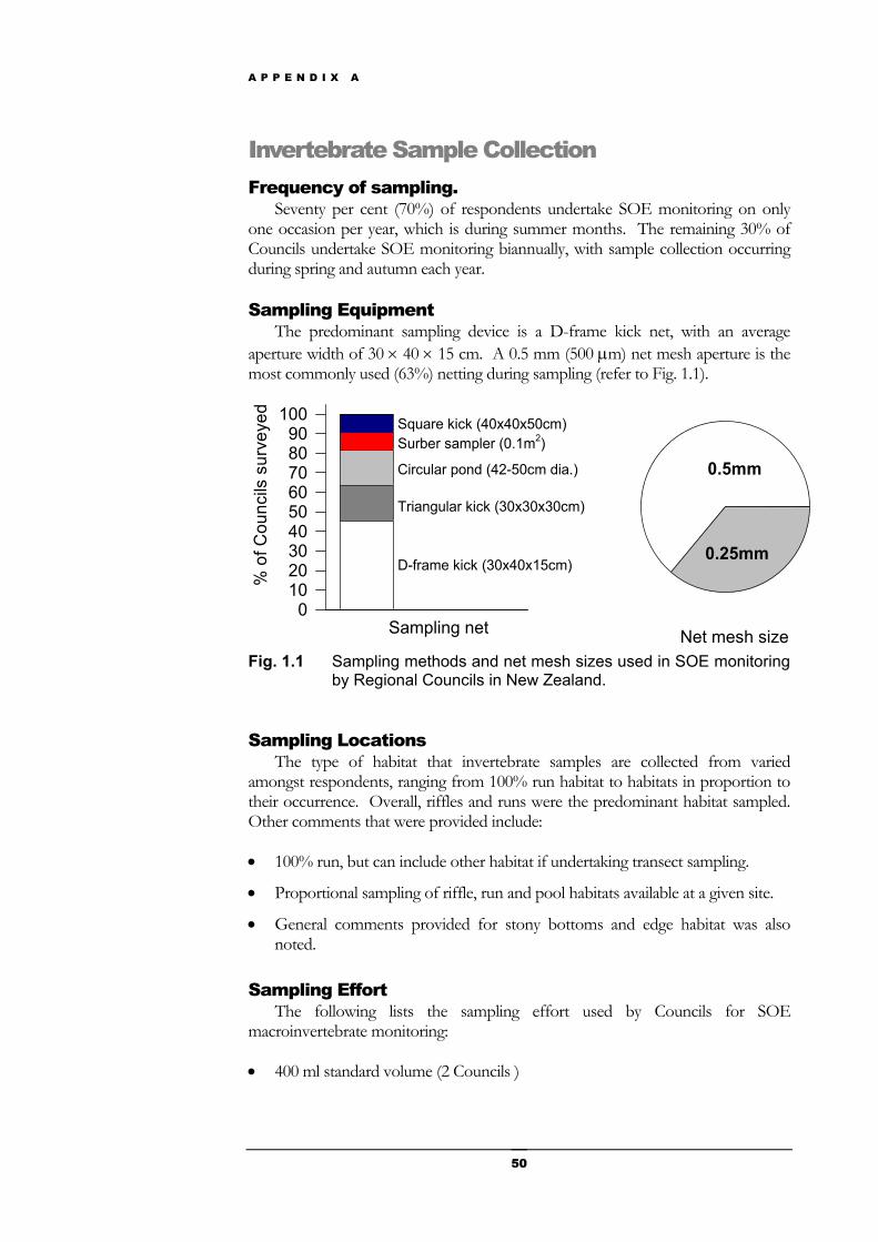
A P P E N D I X A
50
Invertebrate Sample Collection Frequency of sampling.
Seventy per cent (70%) of respondents undertake SOE monitoring on only one occasion per year, which is during summer months. The remaining 30% of Councils undertake SOE monitoring biannually, with sample collection occurring during spring and autumn each year.
Sampling Equipment The predominant sampling device is a D-frame kick net, with an average
aperture width of 30 × 40 × 15 cm. A 0.5 mm (500 µm) net mesh aperture is the most commonly used (63%) netting during sampling (refer to Fig. 1.1).
Sampling net
% o
f Cou
ncils
sur
veye
d
0102030405060708090
100
D-frame kick (30x40x15cm)
Triangular kick (30x30x30cm)
Circular pond (42-50cm dia.)
Surber sampler (0.1m2)Square kick (40x40x50cm)
Net mesh size
0.5mm
0.25mm
Fig. 1.1 Sampling methods and net mesh sizes used in SOE monitoring
by Regional Councils in New Zealand.
Sampling Locations The type of habitat that invertebrate samples are collected from varied
amongst respondents, ranging from 100% run habitat to habitats in proportion to their occurrence. Overall, riffles and runs were the predominant habitat sampled. Other comments that were provided include:
• 100% run, but can include other habitat if undertaking transect sampling.
• Proportional sampling of riffle, run and pool habitats available at a given site.
• General comments provided for stony bottoms and edge habitat was also noted.
Sampling Effort The following lists the sampling effort used by Councils for SOE
macroinvertebrate monitoring:
• 400 ml standard volume (2 Councils )
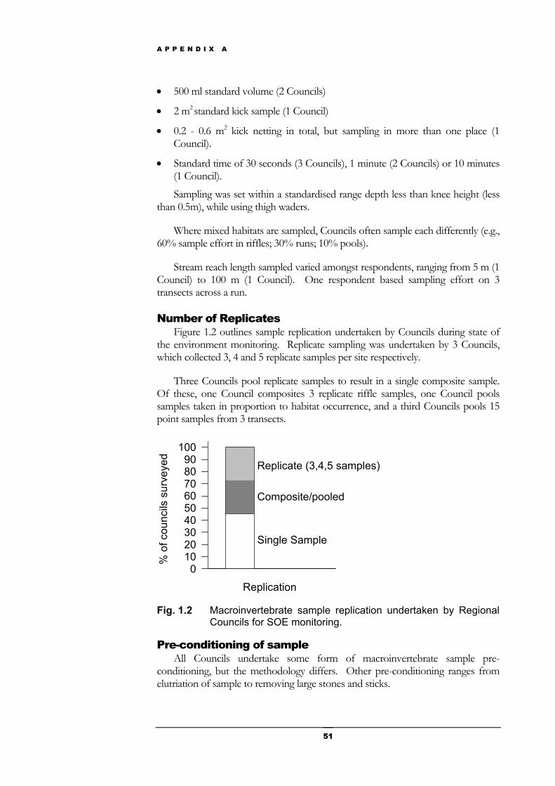
A P P E N D I X A
51
• 500 ml standard volume (2 Councils)
• 2 m2 standard kick sample (1 Council)
• 0.2 - 0.6 m2 kick netting in total, but sampling in more than one place (1 Council).
• Standard time of 30 seconds (3 Councils), 1 minute (2 Councils) or 10 minutes (1 Council).
Sampling was set within a standardised range depth less than knee height (less than 0.5m), while using thigh waders.
Where mixed habitats are sampled, Councils often sample each differently (e.g., 60% sample effort in riffles; 30% runs; 10% pools).
Stream reach length sampled varied amongst respondents, ranging from 5 m (1 Council) to 100 m (1 Council). One respondent based sampling effort on 3 transects across a run.
Number of Replicates Figure 1.2 outlines sample replication undertaken by Councils during state of
the environment monitoring. Replicate sampling was undertaken by 3 Councils, which collected 3, 4 and 5 replicate samples per site respectively.
Three Councils pool replicate samples to result in a single composite sample. Of these, one Council composites 3 replicate riffle samples, one Council pools samples taken in proportion to habitat occurrence, and a third Councils pools 15 point samples from 3 transects.
Replication
% o
f cou
ncils
sur
veye
d
0102030405060708090
100Replicate (3,4,5 samples)
Composite/pooled
Single Sample
Fig. 1.2 Macroinvertebrate sample replication undertaken by Regional
Councils for SOE monitoring.
Pre-conditioning of sample All Councils undertake some form of macroinvertebrate sample pre-
conditioning, but the methodology differs. Other pre-conditioning ranges from elutriation of sample to removing large stones and sticks.
A P P E N D I X A
52
Environmental conditions prior to sampling All respondents take account of the environmental conditions prior to
sampling. Clear criteria were supplied in most cases as follows:
• No sampling within 3 weeks of flood.
• No sampling within 4 weeks of flood.
• No sampling within 10 days if 7x median flow, nor within 7 days if 3x median flow.
• No sampling within 4 weeks of flood with return period > 5 years, nor within 2 weeks of annual return period.
Transportation and Storage The following provides a list of general comments related to the transportation
and storage of invertebrate samples by Councils:
• Samples are transported preserved (72% of Councils) or in chillybins with ice (1 Council) before sorting.
• Samples are preserved with ethanol (43% of Councils), ethanol/methanol (43%) or formalin (14%).
• Samples are stored for 2 weeks to 6 months prior to sorting.
• Samples are retained indefinitely by 63% of Councils while the remaining Councils (37%) store their sorted samples for approximately 2 years before disposal.
All invertebrates are stored in labelled vials, but it was unclear how long these vials were kept, or where the labelling occurred (i.e., lid, side of container, paper inside). Invertebrate storage ranged from only 3 individuals of each taxon to all individuals sorted per sample.
Storage containers ranged from screwtop containers to small pottles.
Sample Processing Sieving
Four respondents elutriate the invertebrate samples in the field prior to preservation. The remaining 7 Councils made no comment regarding elutriation. Samples were returned to the laboratory for sieving using:
• Single sieve of 0.5 mm mesh (3 Councils).
• A series of sieves: 2.0, 1.0 and 0.5 mm mesh (1 Council); 4.0, 1.0 and 0.5 mm mesh (1 Council); 2.0 and 0.25 mm (2 Councils).
• Single 1mm mesh sieve (1 Council).
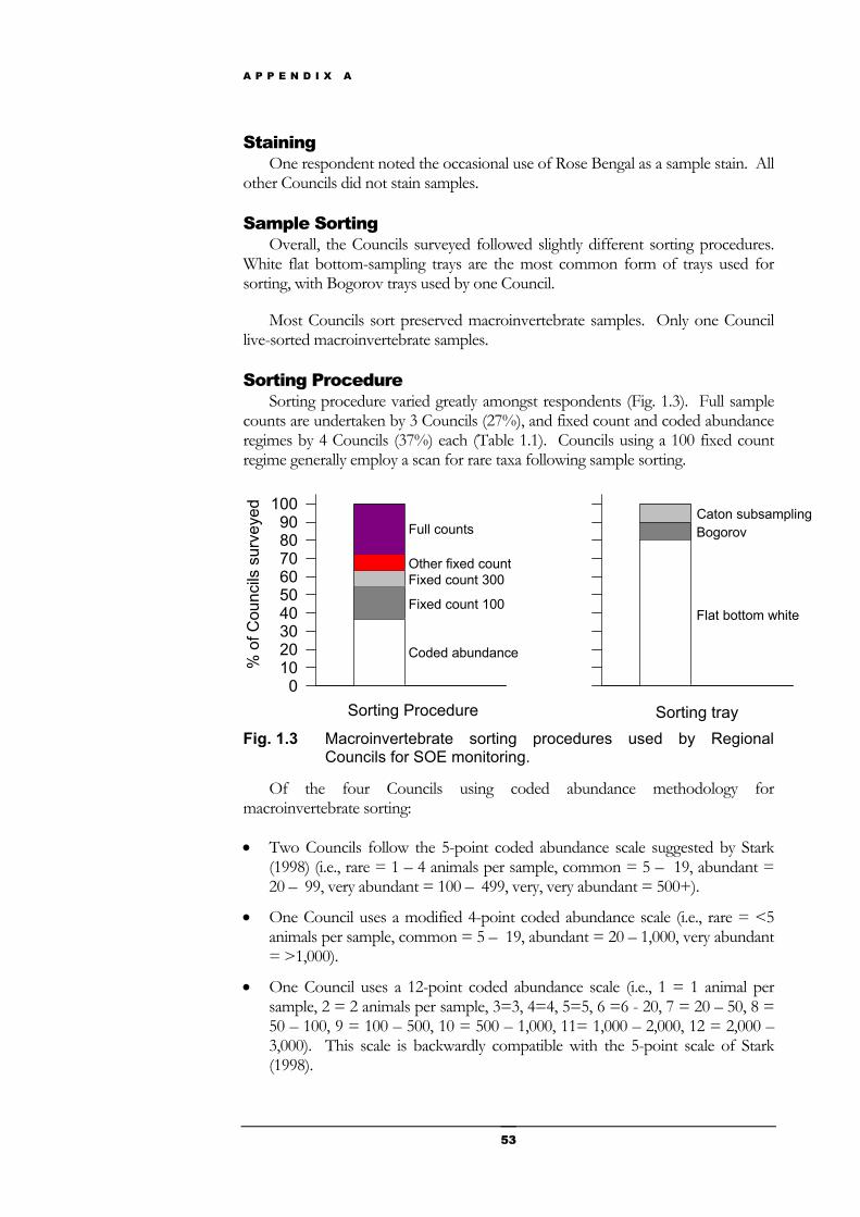
A P P E N D I X A
53
Staining One respondent noted the occasional use of Rose Bengal as a sample stain. All
other Councils did not stain samples.
Sample Sorting Overall, the Councils surveyed followed slightly different sorting procedures.
White flat bottom-sampling trays are the most common form of trays used for sorting, with Bogorov trays used by one Council.
Most Councils sort preserved macroinvertebrate samples. Only one Council live-sorted macroinvertebrate samples.
Sorting Procedure Sorting procedure varied greatly amongst respondents (Fig. 1.3). Full sample
counts are undertaken by 3 Councils (27%), and fixed count and coded abundance regimes by 4 Councils (37%) each (Table 1.1). Councils using a 100 fixed count regime generally employ a scan for rare taxa following sample sorting.
Sorting Procedure
% o
f Cou
ncils
sur
veye
d
0102030405060708090
100
Coded abundance
Fixed count 100
Fixed count 300Other fixed count
Full counts
Sorting tray
Flat bottom white
BogorovCaton subsampling
Fig. 1.3 Macroinvertebrate sorting procedures used by Regional
Councils for SOE monitoring.
Of the four Councils using coded abundance methodology for macroinvertebrate sorting:
• Two Councils follow the 5-point coded abundance scale suggested by Stark (1998) (i.e., rare = 1 – 4 animals per sample, common = 5 – 19, abundant = 20 – 99, very abundant = 100 – 499, very, very abundant = 500+).
• One Council uses a modified 4-point coded abundance scale (i.e., rare = <5 animals per sample, common = 5 – 19, abundant = 20 – 1,000, very abundant = >1,000).
• One Council uses a 12-point coded abundance scale (i.e., 1 = 1 animal per sample, 2 = 2 animals per sample, 3=3, 4=4, 5=5, 6 =6 - 20, 7 = 20 – 50, 8 = 50 – 100, 9 = 100 – 500, 10 = 500 – 1,000, 11= 1,000 – 2,000, 12 = 2,000 – 3,000). This scale is backwardly compatible with the 5-point scale of Stark (1998).
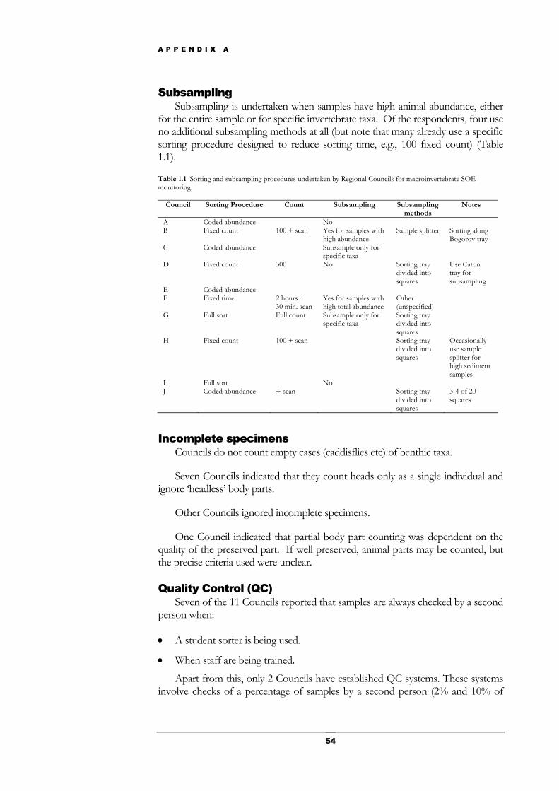
A P P E N D I X A
54
Subsampling Subsampling is undertaken when samples have high animal abundance, either
for the entire sample or for specific invertebrate taxa. Of the respondents, four use no additional subsampling methods at all (but note that many already use a specific sorting procedure designed to reduce sorting time, e.g., 100 fixed count) (Table 1.1).
Table 1.1 Sorting and subsampling procedures undertaken by Regional Councils for macroinvertebrate SOE monitoring.
Council Sorting Procedure Count Subsampling Subsampling methods
Notes
A Coded abundance No B Fixed count 100 + scan Yes for samples with
high abundance Sample splitter Sorting along
Bogorov tray C Coded abundance Subsample only for
specific taxa
D Fixed count 300 No Sorting tray divided into squares
Use Caton tray for subsampling
E Coded abundance F Fixed time 2 hours +
30 min. scan Yes for samples with high total abundance
Other (unspecified)
G Full sort Full count Subsample only for specific taxa
Sorting tray divided into squares
H Fixed count 100 + scan Sorting tray divided into squares
Occasionally use sample splitter for high sediment samples
I Full sort No J Coded abundance + scan Sorting tray
divided into squares
3-4 of 20 squares
Incomplete specimens Councils do not count empty cases (caddisflies etc) of benthic taxa.
Seven Councils indicated that they count heads only as a single individual and ignore ‘headless’ body parts.
Other Councils ignored incomplete specimens.
One Council indicated that partial body part counting was dependent on the quality of the preserved part. If well preserved, animal parts may be counted, but the precise criteria used were unclear.
Quality Control (QC) Seven of the 11 Councils reported that samples are always checked by a second
person when:
• A student sorter is being used.
• When staff are being trained.
Apart from this, only 2 Councils have established QC systems. These systems involve checks of a percentage of samples by a second person (2% and 10% of
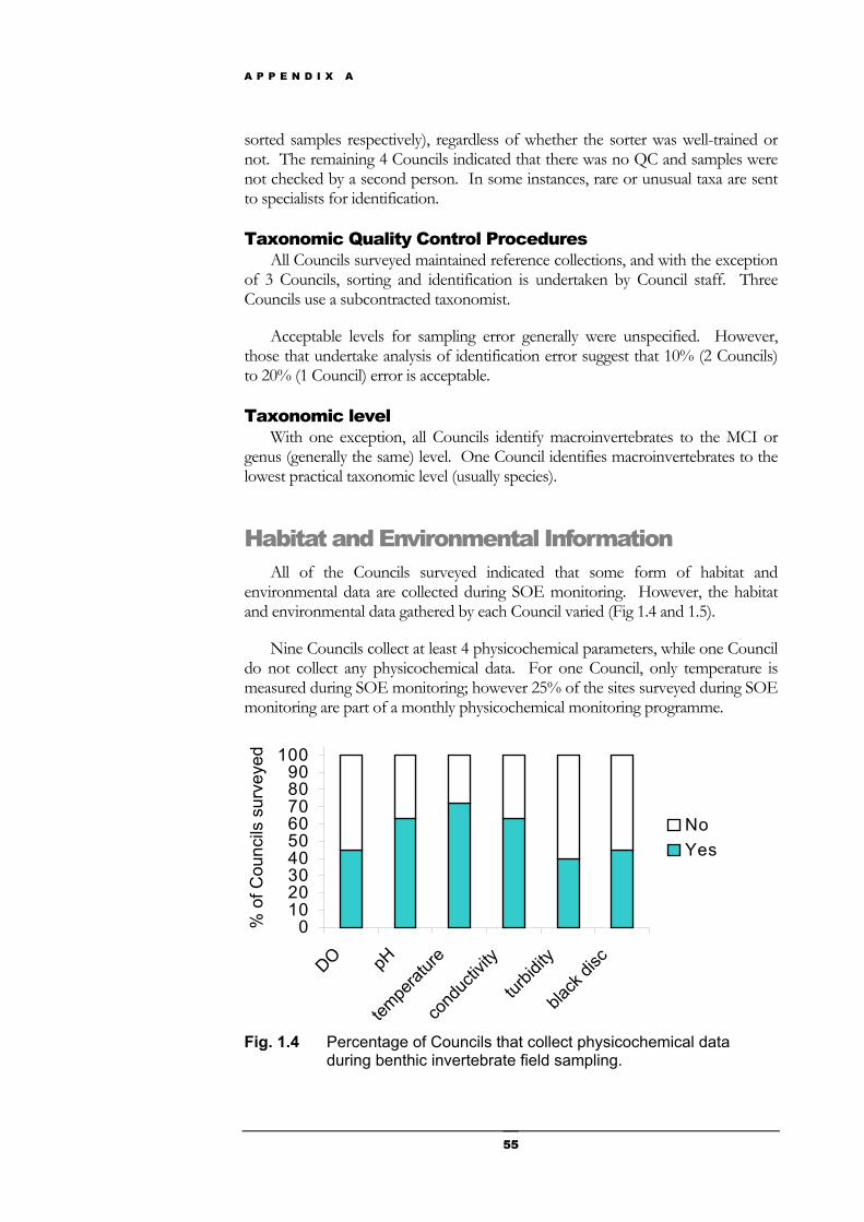
A P P E N D I X A
55
sorted samples respectively), regardless of whether the sorter was well-trained or not. The remaining 4 Councils indicated that there was no QC and samples were not checked by a second person. In some instances, rare or unusual taxa are sent to specialists for identification.
Taxonomic Quality Control Procedures All Councils surveyed maintained reference collections, and with the exception
of 3 Councils, sorting and identification is undertaken by Council staff. Three Councils use a subcontracted taxonomist.
Acceptable levels for sampling error generally were unspecified. However, those that undertake analysis of identification error suggest that 10% (2 Councils) to 20% (1 Council) error is acceptable.
Taxonomic level With one exception, all Councils identify macroinvertebrates to the MCI or
genus (generally the same) level. One Council identifies macroinvertebrates to the lowest practical taxonomic level (usually species).
Habitat and Environmental Information All of the Councils surveyed indicated that some form of habitat and
environmental data are collected during SOE monitoring. However, the habitat and environmental data gathered by each Council varied (Fig 1.4 and 1.5).
Nine Councils collect at least 4 physicochemical parameters, while one Council do not collect any physicochemical data. For one Council, only temperature is measured during SOE monitoring; however 25% of the sites surveyed during SOE monitoring are part of a monthly physicochemical monitoring programme.
0102030405060708090
100
DO pH
tempe
rature
cond
uctiv
ity
turbid
ity
black
disc
% o
f Cou
ncils
sur
veye
d
NoYes
Fig. 1.4 Percentage of Councils that collect physicochemical data
during benthic invertebrate field sampling.
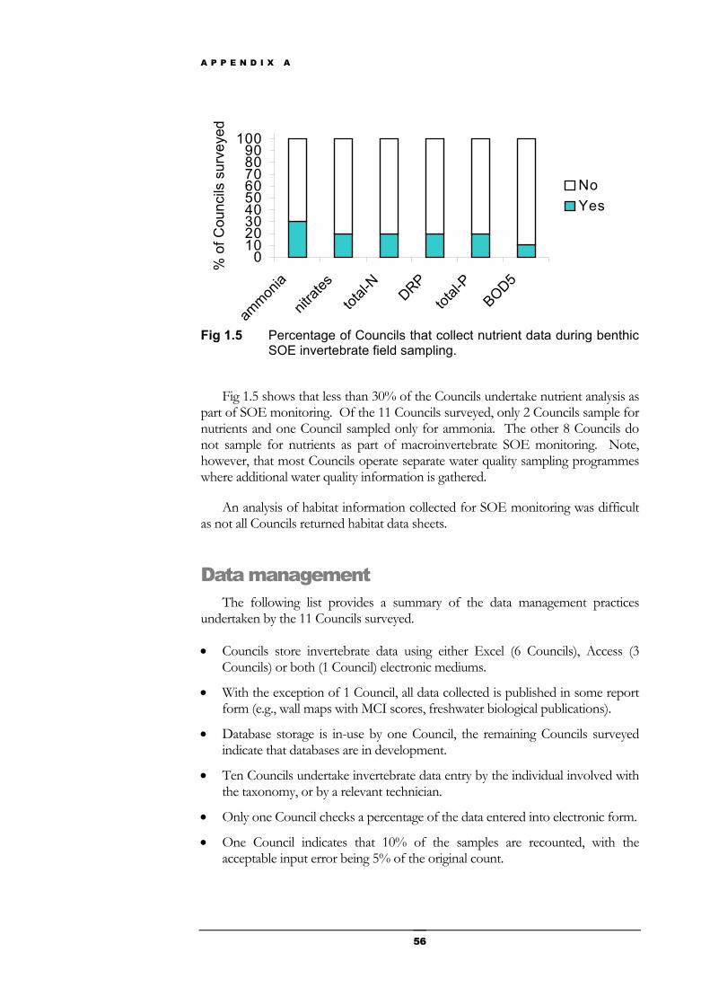
A P P E N D I X A
56
0102030405060708090
100
ammon
ia
nitrat
es
total-
NDRP
total-
PBOD5
% o
f Cou
ncils
sur
veye
d
NoYes
Fig 1.5 Percentage of Councils that collect nutrient data during benthic
SOE invertebrate field sampling.
Fig 1.5 shows that less than 30% of the Councils undertake nutrient analysis as part of SOE monitoring. Of the 11 Councils surveyed, only 2 Councils sample for nutrients and one Council sampled only for ammonia. The other 8 Councils do not sample for nutrients as part of macroinvertebrate SOE monitoring. Note, however, that most Councils operate separate water quality sampling programmes where additional water quality information is gathered.
An analysis of habitat information collected for SOE monitoring was difficult as not all Councils returned habitat data sheets.
Data management The following list provides a summary of the data management practices
undertaken by the 11 Councils surveyed.
• Councils store invertebrate data using either Excel (6 Councils), Access (3 Councils) or both (1 Council) electronic mediums.
• With the exception of 1 Council, all data collected is published in some report form (e.g., wall maps with MCI scores, freshwater biological publications).
• Database storage is in-use by one Council, the remaining Councils surveyed indicate that databases are in development.
• Ten Councils undertake invertebrate data entry by the individual involved with the taxonomy, or by a relevant technician.
• Only one Council checks a percentage of the data entered into electronic form.
• One Council indicates that 10% of the samples are recounted, with the acceptable input error being 5% of the original count.
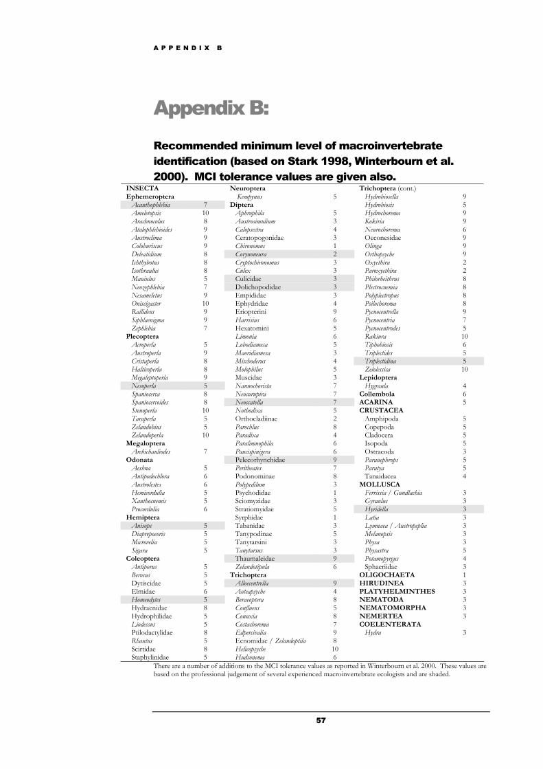
A P P E N D I X B
57
Appendix B: Recommended minimum level of macroinvertebrate identification (based on Stark 1998, Winterbourn et al. 2000). MCI tolerance values are given also.
INSECTA Neuroptera Trichoptera (cont.) Ephemeroptera Kempynus 5 Hydrobiosella 9 Acanthophlebia 7 Diptera Hydrobiosis 5 Ameletopsis 10 Aphrophila 5 Hydrochorema 9 Arachnocolus 8 Austrosimulium 3 Kokiria 9 Atalophlebioides 9 Calopsectra 4 Neurochorema 6 Austroclima 9 Ceratopogonidae 3 Oeconesidae 9 Coloburiscus 9 Chironomus 1 Olinga 9 Deleatidium 8 Corynoneura 2 Orthopsyche 9 Ichthybotus 8 Cryptochironomus 3 Oxyethira 2 Isothraulus 8 Culex 3 Paroxyethira 2 Mauiulus 5 Culicidae 3 Philorheithrus 8 Neozephlebia 7 Dolichopodidae 3 Plectrocnemia 8 Nesameletus 9 Empididae 3 Polyplectropus 8 Oniscigaster 10 Ephydridae 4 Psilochorema 8 Rallidens 9 Eriopterini 9 Pycnocentrella 9 Siphlaenigma 9 Harrisius 6 Pycnocentria 7 Zephlebia 7 Hexatomini 5 Pycnocentrodes 5 Plecoptera Limonia 6 Rakiura 10 Acroperla 5 Lobodiamesa 5 Tiphobiosis 6 Austroperla 9 Maoridiamesa 3 Triplectides 5 Cristaperla 8 Mischoderus 4 Triplectidina 5 Halticoperla 8 Molophilus 5 Zelolessica 10 Megaleptoperla 9 Muscidae 3 Lepidoptera Nesoperla 5 Nannochorista 7 Hygraula 4 Spaniocerca 8 Neocurupira 7 Collembola 6 Spaniocercoides 8 Neoscatella 7 ACARINA 5 Stenoperla 10 Nothodixa 5 CRUSTACEA Taraperla 5 Orthocladiinae 2 Amphipoda 5 Zelandobius 5 Parochlus 8 Copepoda 5 Zelandoperla 10 Paradixa 4 Cladocera 5 Megaloptera Paralimnophila 6 Isopoda 5 Archichauliodes 7 Paucispinigera 6 Ostracoda 3 Odonata Pelecorhynchidae 9 Paranephrops 5 Aeshna 5 Peritheates 7 Paratya 5 Antipodochlora 6 Podonominae 8 Tanaidacea 4 Austrolestes 6 Polypedilum 3 MOLLUSCA Hemicordulia 5 Psychodidae 1 Ferrissia / Gundlachia 3 Xanthocnemis 5 Sciomyzidae 3 Gyraulus 3 Procordulia 6 Stratiomyidae 5 Hyridella 3 Hemiptera Syrphidae 1 Latia 3 Anisops 5 Tabanidae 3 Lymnaea / Austropeplia 3 Diaprepocoris 5 Tanypodinae 5 Melanopsis 3 Microvelia 5 Tanytarsini 3 Physa 3 Sigara 5 Tanytarsus 3 Physastra 5 Coleoptera Thaumaleidae 9 Potamopyrgus 4 Antiporus 5 Zelandotipula 6 Sphaeriidae 3 Berosus 5 Trichoptera OLIGOCHAETA 1 Dytiscidae 5 Alloecentrella 9 HIRUDINEA 3 Elmidae 6 Aoteapsyche 4 PLATYHELMINTHES 3 Homeodytes 5 Beraeoptera 8 NEMATODA 3 Hydraenidae 8 Confluens 5 NEMATOMORPHA 3 Hydrophilidae 5 Conuxia 8 NEMERTEA 3 Liodessus 5 Costachorema 7 COELENTERATA Ptilodactylidae 8 Edpercivalia 9 Hydra 3 Rhantus 5 Ecnomidae / Zelandoptila 8 Scirtidae 8 Helicopsyche 10 Staphylinidae 5 Hudsonema 6
There are a number of additions to the MCI tolerance values as reported in Winterbourn et al. 2000. These values are based on the professional judgement of several experienced macroinvertebrate ecologists and are shaded.