Embed Size (px)
Citation preview
Journal of Economics and Business 62 (2010) 94–115
Contents lists available at ScienceDirect
Journal of Economics and Business
Quality requirements in developing countries
Galina Ana,∗, Thitima Puttitanunb
a 304 Ascension Hall, Economics Department, Kenyon College, Gambier, OH 43022, United Statesb Department of Economics, San Diego State University, 5500 Campanile Dr., San Diego, CA 92182, United States
a r t i c l e i n f o
Article history:Received 20 February 2008Received in revised form 14 May 2009Accepted 7 August 2009
Keywords:Quality requirementsTechnological changeMultinational firmsDeveloping countries
a b s t r a c t
This paper theoretically explores how quality standards imposedby subsidiaries of multinational enterprises on local suppliers indeveloping countries can influence the local intermediate goodsindustries: they can trigger the adoption of better techniques andprocesses, thereby increasing the technological capability of thehost country; they can also induce local innovation, a situationdescribed in many case studies of developing countries. However,if a host country is underdeveloped, the presence of multinationalfirms might not bring any significant changes to the economy.
Published by Elsevier Inc.
1. Introduction
The presence of multinational enterprises (MNEs) in developing countries is increasingly consid-ered beneficial to host economies. The literature suggests several sources of positive influence fromforeign direct investment (FDI). First, technological spillovers from FDI could occur in the form oflocal producers observing, learning from, and imitating more advanced technologies, adopting bettermanagement practices of MNEs (Blomström & Kokko, 1998; Mansfield & Romeo, 1980). In addition,MNEs often help to augment the value of local human capital by providing substantial training to localemployees (Brash, 1966; Hobday, 1995; Katz, 1987). Finally, MNE subsidiaries can influence the pro-ductivity of local producers through linkages with domestic suppliers (backward linkages) and clientsor distributors (forward linkages) (Lall, 1980; McAleese & McDonald, 1978).
This paper explores another channel of potential positive influence from multinationals operatingin developing countries: quality upgrading as a result of standards imposed by MNEs on local suppliersof intermediate goods. The recent melamine scare in pet food, toys, tires, seafood, pharmaceuticals,
∗ Corresponding author. Tel.: +1 619 594 3556; fax: +1 619 594 5062.E-mail addresses: [email protected] (G. An), [email protected] (T. Puttitanun).
0148-6195/$ – see front matter. Published by Elsevier Inc.doi:10.1016/j.jeconbus.2009.08.001
G. An, T. Puttitanun / Journal of Economics and Business 62 (2010) 94–115 95
and toothpaste industries that procure their supplies from China highlights the importance of qualitystandards in the ability of developing countries’ firms to sell their products globally. A simple modeldeveloped below analyzes how quality requirements and demand from multinational firms mightinduce local suppliers to invest in product quality, which in turn can lead to higher productivity inother industries. The decision to improve quality is influenced by the profitability of the venture, whichin turn depends on the prices of final and intermediate goods, investment costs, and the content oflocal input into MNE production. In addition, the capacity of local suppliers to absorb knowledge alsoinfluences the level of investment and their ability to innovate. The model allows for the possibilitythat local suppliers can improve the intermediate product via innovation, as well as a situation whereMNE’s entry has no impact on the local intermediate goods industry. Since the focus of the paper ispotential externalities from activities of multinational enterprises in developing countries, we are notconcerned with the welfare of global consumers; in addition, we limit our analysis to cases when theoriginal demand for the product that the MNE produces does not exist in the host country—a typicalsituation for many developing countries.1
The rest of the paper is organized as follows: Section 2 describes the related literature, Section 3presents the model, Section 4 analyzes the effects of MNE presence on the local economy, and Section5 concludes the paper.
2. Related literature
Most theoretical studies on technological externalities arising from the presence of MNEs modelthem as “contagion effects” (Baldwin, Braconier, & Forslid, 1999; Das, 1987; Findlay, 1978). Fosfuri,Motta, and Ronde (2001) and Markusen (2001) address the knowledge spillovers that occur when localemployees trained by a multinational firm leave the company and work for a domestic enterprise.Some other work has been conducted on modeling linkages between multinational firms and localproducers. In particular, Rodriguez-Clare (1996) examines how such linkages affect wages, the varietyof intermediate inputs produced within the economy, and the economic development of the hostcountry. Markusen and Venables (1999) examine the interaction between the competition effect,which refers to the substitution of domestic for multinational production in the downstream industry,and the linkage effect, which refers to an increase in demand for local intermediates. The work belowhighlights another novel channel of technological improvements in the form of quality upgradingwithin upstream industries in developing countries as a result of linkages between multinationalenterprises and local suppliers.
The available empirical work addresses the existence of positive spillovers from the presenceof multinational enterprises, though it does not disentangle the effects on firms’ productivity fromthe various sources of spillovers. Görg and Strobl (2001) examine existing empirical studies onhorizontal spillovers (spillovers that arise from the presence of multinational enterprises in thesame industry) and indicate that the impact on the productivity of domestic firms is inconclusive.Studies that use cross-section data (see, among others, Blomström & Persson, 1983; Blomström& Wolff, 1994; Caves, 1974; Chuang & Lin, 1999; Kokko, 1994, 1996) usually find evidence ofpositive spillovers, while those that use panel data (see, for instance, Aitken & Harrison, 1999;Djankov & Hoekman, 2000; Haddad & Harrison, 1993) find negative or statistically insignificanteffects of FDI. Positive horizontal externalities, however, were reported for industrial countriesby Haskel, Pereira, and Slaughter (2002) and Keller and Yeaple (2003) for the United Kingdomand the United States, respectively. Other authors (see, for instance, Blalock, 2001; Blalock &Gertler, 2008; Schoors & van der Tol, 2002; Smarzynska, 2004) point out that positive spillovers
1 The bulk of foreign direct investment in developing countries is undertaken by multinationals in search of low productioncosts rather than local demand for their goods (Vernon (1966)). For example, in the 1960s, U.S. electronics firms in Taiwanproduced mostly for export, Singer (a sewing machine company) in Taiwan exported around 90% of its production in the1970s, and electronics output carried out by large multinational firms in Singapore was mostly for exports (Hobday, 1995;Schive, 1990). Blalock and Gertler (2008) note that most multinational firms in Indonesia are export-oriented and generally donot supply to Indonesian customers. Similar examples can be found in countries such as Mexico, Brazil, and Thailand (Moran(1998)).
96 G. An, T. Puttitanun / Journal of Economics and Business 62 (2010) 94–115
are more likely to arise when MNEs are dealing with their suppliers (through backward link-ages) or customers (through forward linkages)—so-called vertical externalities. Smarzynska providesconvincing evidence of positive productivity spillovers taking place via backward linkages in Lithua-nia, while Blalock and Gertler find evidence of productivity gains, greater competition, and lowerprices among domestic suppliers to multinationals in Indonesian manufacturing industries. Theyalso detect positive externalities from the supply sector to other downstream producers. Schoorsand van der Tol use Hungarian firm-level data to show positive vertical FDI spillovers in thatcountry.
As mentioned above, the available empirical studies do not differentiate between the varioussources of externalities. In particular, it is unclear whether technical/financial support, quality require-ments, or other factors contribute to the increased productivity of domestic suppliers of multinationalfirms. The only evidence of the improved performance of local producers as a result of quality require-ments from MNEs can be discerned from a number of case studies. In a survey paper, Blomström andKokko (1998) cite studies by Brash (1966, pp. 124–125, 201–202), Katz (1969, p. 154), and Watanabe(1983, pp. 116, 121–122) in Australia, Argentina, and the Philippines, respectively, that describe strictMNE requirements for product quality, characteristics, and reliability, imposed on local suppliers, thatin turn had positive effects on their choices of technologies, productive processes, and techniques.Hobday (1995, pp. 66–67) also observed that local suppliers in East Asia had to produce intermediateinputs of the highest quality at the lowest price. Surprisingly, compliance with the quality standardshad led to better performances by local suppliers in other, unrelated operations. An interesting phe-nomenon described in the case studies is that increased demand for local production could inducelocal suppliers to invest in the development of better products and processes. Katz (1987, pp. 41–42,218–219) shows that domestic suppliers in a number of Latin American countries would often redesignparts and components to increase resistance and improve performance. Lall (1980) describes a case inIndia where one of the projects of a domestic supplier was so successful that the MNE subsidiary triedto persuade its parent to adopt it at home. Other remarkable examples can be found in case studiesof East Asian economies, where local firms started by supplying parts to subsidiaries of multinationalenterprises in the electronics, bicycle, and sewing machine industries, but later became independentin creating their own designs and products (Hobday, 1995, pp. 116–119, 176–177). Some of themtook over the whole industry and learned to export directly to Western markets (Hobday, 1995, pp.123–132).
The model below examines scenarios wherein the local supplier either chooses to improvethe quality of his products and sell them to both local and multinational producers, or tokeep producing lower quality intermediate goods and supply them to a domestic produceronly. It also shows that expanding demand for domestic production can lead to local innova-tions.
We believe that this paper can also be viewed within the broader context of the general quest foreconomic growth in developing countries (see, for instance, Aghion and Howitt (1998), Temple (1999)).Recent work on compliance with quality standards in poor nations (Henson & Mitullah, 2004; Jaffee &Henson, 2004; Stanford, 2002) suggests that adopting stricter standards can improve countries’ exportperformances and serve as a catalyst for growth and development. This paper contributes to the aboveliterature by examining a similar venue through quality upgrading that could significantly contributeto poor nations’ growth performance and should be considered by developing countries’ governmentsin their policy decision-making.
2.1. The model
Consider a small developing country that can produce a low-technology good L, but does not haveadequate knowledge to produce a high-technology good H.2 The production of the low-tech good L(the downstream industry) requires intermediates x (of any quality) that can either be produced by
2 We assume that goods L and H are not related. For example, an increase in the demand for computers does not influencethe demand for radios.
G. An, T. Puttitanun / Journal of Economics and Business 62 (2010) 94–115 97
the local producers of intermediates (the upstream industry) or imported. The upstream industry ischaracterized by Bertrand competition, so only the lowest-cost producer(s) will be operating in theindustry. Assume that there is a single producer of intermediate goods with the lowest productioncosts that will charge a price that will undercut domestic as well as foreign competitors.3 High-techgood H cannot be produced by local firms due to the absence of technological know-how. In addition,local demand for the good does not exist yet due to either insufficient income or any sort of demandlag.4 However, a subsidiary of a multinational firm (hereafter referred to as an “MNE”) might startdomestic production of the good if it can source local intermediates at lower prices (or, alternatively,outsource the production of some parts to the low-cost local suppliers). In that case, the local suppliershave to upgrade their facilities to produce high-quality intermediates for the MNE that satisfy therequired quality standards.5 The upgraded facilities also improve the quality of the intermediate goodsupplied to the domestic downstream producer.6 The alternative for the MNE is to buy intermediatesin the global market. We assume that the MNE can also enter the local upstream industry, but thecosts of production will exceed those of local producers due to the MNE’s unfamiliarity with domesticconditions.7,8
2.2. Basic notation
Qd quantity of the low-tech product L produced by the domestic manufacturerQm quantity of the high-tech good H produced by the MNEPd price of the low-tech good L produced by the local manufacturerPm price of the high-tech good H produced by the MNE˘d profits of the final domestic manufacturer˘m profits of the MNExd
ilocal producer’s demand for the low-tech intermediate good
xmi
MNE’s demand for the high-tech intermediate goodpL
ilocal price of the low-tech intermediate good
pHi
local price of the high-tech intermediate goodpL the lowest price of the low-tech intermediates that could be charged by domestic and foreign
competitorspH the lowest price of the high-tech intermediates that could be charged by domestic and foreign
competitors�d profits of the intermediate manufacturer from supply to the domestic company�m profits of the intermediate manufacturer from supply to both the domestic company and the
MNE�i quality of the intermediate goods� threshold level of quality required by the MNEi effort level invested in quality improvements by the local supplier9
i effort level necessary to achieve threshold quality level �f investment cost of the local supplier per unit of effortc incumbent’s marginal cost of producing the intermediate goods
3 This assumption is not unrealistic since many manufacturing industries in developing countries are dominated by largeproducers.
4 See endnote 11 for explanations. For the demand lag hypothesis, see, for instance, Posner (1961).5 Alternatively, the government of the host country might set up trading companies to facilitate the export of goods that
satisfy world quality standards abroad. However, this strategy might require very high marketing costs.6 The intermediates supplied to the MNE and to the domestic firm are two different goods. However, if the local producer
improves the quality of the intermediate product supplied to the MNE, the quality of the product supplied to the domesticcompany can be improved with no additional cost.
7 In a trivial case where the MNE has lower production cost due to some sort of firm-specific assets (see, for instance, Caves(1996)), it might drive the upstream producer out of business completely.
8 Note that uppercase letters in notations correspond to the final goods producers, while lowercase letters correspond to theintermediate goods producer.
9 The reason letter i is used to denote both the effort level and a subscript for the quality of intermediates is explained below.
98 G. An, T. Puttitanun / Journal of Economics and Business 62 (2010) 94–115
2.3. The final good (downstream) industry
The domestic producer of the final good needs xdi
intermediates to produce the low-tech good L inthe amount of Qd. Index d refers to the domestic downstream producer, and index i refers to differentlevels of quality, �i, of the intermediate goods. We denote �1 ≡ 1 as the minimum quality of the good,which can be improved by investing effort i to obtain a higher quality level �i > 1. In particular, weassume that �i =
√i, where i ≥ 1. Quality �i is an increasing and concave function of effort i since it is
easier to improve a lower quality good than a higher quality one.10
The local downstream producer has a Cobb–Douglas production function that depends on quality�i of the intermediate inputs:
Qd = 1˛
�1−˛i
(xdi )
˛where 0 < ˛ < 1. (1)
Note that better-quality intermediates generate higher outputs. Since the country is small and opento trade in final goods, the domestic downstream producer faces price Pd for his good. The producermaximizes profit:∏
d= PdQd − pL
i xdi (2)
where pLi
is the price of the low-tech intermediate good charged either by the local upstream produceror by world suppliers. Substituting (1) into (2) and maximizing it with respect to xd
iyields the domestic
demand for low-tech intermediates as a function of quality �i. and the price of intermediate good pLi:
xdi = �i
(Pd
pLi
)1/(1−˛)
(3)
The MNE has an analogous production function in the host country:
Qm =
⎧⎨⎩
1ˇ
�1−ˇi
(xmi )ˇ for �i ≥ �
0 otherwise, (4)
where 0 < ˇ < 1 and xmi
are the intermediates of quality level � or higher for the high-tech good H. Theparameter ˇ represents the content of intermediate inputs in the production of the final good. In thecase where the MNE buys intermediate goods from local suppliers, a higher ˇ means higher demandfor the local good. As stated above, there is a threshold quality level �, � > 1, of the intermediate goodsrequired by the MNE. The local firm will need to invest effort i in order to achieve quality �.
The MNE maximizes the following profit function:∏m
= PmQm − pHi xm
i (5)
Substituting (4) into (5) and maximizing it with respect to xmi
yields the MNE’s demand for high-qualityintermediates:
xmi = �i
(Pm
pHi
)1/(1−ˇ)
(6)
2.4. The intermediate goods (upstream) producer
A domestic producer of intermediate goods has two options in the presence of the MNE. The firstis to produce a low-tech intermediate good (�i < �) for the local downstream producer only. The
10 For the sake of convenience, the letter i is used to denote both the amount of effort and the quality level subscript of theintermediate good since effort i determines the quality �i . For example, investing two units of effort results in upgrading qualityto �2 =
√2.
G. An, T. Puttitanun / Journal of Economics and Business 62 (2010) 94–115 99
second option is to upgrade his facilities, produce the high-quality intermediates (�i < �) required bythe MNE, and supply to both downstream firms.11 To upgrade the facilities and improve quality, theproducer has to invest effort i, which costs f per unit of effort.12 Investment costs will then be a linearfunction of effort: f × i. With upgraded facilities, the quality of both types of intermediates increases.
Let us first assume that the local supplier produces only for the domestic downstream firm (�i < �).In this case, he faces the demand for his good xd
iand determines the price pL
i. He will either charge
a profit-maximizing price, pLmax, or the highest possible price that will undercut his competitors
domestically and abroad, pL , i.e., pLi
= min{pLmax, pL}.
His profit function is given by
�d = pLi xd
i − cxdi − fi = (pL
i − c)xdi − fi, (7)
where c is the constant marginal cost of producing intermediates and fi is the investment cost. Sub-stituting the demand equation for domestic intermediates (3) into (7) yields:
�d = �i
(pL
i − c)(Pd
pLi
)1/(1−˛)
− fi =√
i(pLi − c)
(Pd
pLi
)1/(1−˛)
− fi (8)
Maximizing (8) with respect to pLi
and i yields the following first-order conditions:
where price pLi
should also satisfy the non-negative profit condition �∗d(pL
i) ≥ 0.
Solutions for (9.1)–(9.4) can be written as follows:13⎧⎪⎨⎪⎩
pL∗i
= min{ c
˛, pL}
i∗ = max{1,(
Vd
2f
)2}
(10)
where
Vd =
⎧⎪⎨⎪⎩
(1 − ˛)(
˛
c
)˛/(1−˛)P1/(1−˛)
dif c/˛ ≤ pL
(pL − c)(
Pd
pL
)1/(1−˛)if pL < c/˛
, (11)
11 See, for instance, Lall (2000), who observes that in many cases, quality upgrading activities are usually not taking placeunless MNEs are involved.
12 We assume that quality improvements involve fixed cost, f, because the bulk of the investment is usually devoted to thepossible restructuring of existing facilities or the construction of new ones, as well as to establishing a monitoring system forsafety, quality, conformity, and plant health; enforcing inspection and certification procedures; upgrading laboratory facilities;training personnel; refinement of the sector’s “codes of practice” and administrative structure; and other related investments.All of those are examples of fixed investment costs. For reference, see Maskus, Otsuki and Wilson (2001), and Hobday (1995,pp. 67, 127, 154).
13 Please see Appendix A for derivations of the FOCs and the SOCs.
100 G. An, T. Puttitanun / Journal of Economics and Business 62 (2010) 94–115
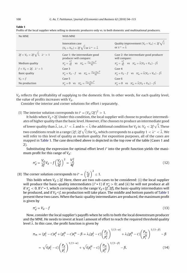
Table 1Profits of the local supplier when selling to domestic producers only vs. to both domestic and multinational producers.
No MNE With MNE
Innovation case
(Vd + Vm) > 2f
√i or �∗∗ > �
Quality improvement (Vd + Vm) < 2f
√i
or �∗∗ = �
2f < Vd < 2f
√i, �∗ > 1 Case 1: the intermediate good
producer will compare:Case 2: the intermediate good producerwill compare:
Medium quality �∗d
= V2d
4 fvs �∗
m = (Vd+Vm)2
4 f�∗
d= V2
d4 f
vs �∗m = �(Vd + Vm) − f i
f < Vd < 2f, �∗ = 1 Case 3 Case 4
Basic quality �∗d
= Vd − f vs �∗m = (Vd+Vm)2
4 f�∗
d= Vd − f vs �∗
m = �(Vd + Vm) − f i
Vd < f Case 5 Case 6
No production �∗d
= 0 vs �∗m = (Vd+Vm)2
4 f�∗
d= 0 vs �∗
m = �(Vd + Vm) − f i
Vd reflects the profitability of supplying to the domestic firm. In other words, for each quality level,the value of profits increases with Vd.
Consider the interior and corner solutions for effort i separately.
(I) The interior solution corresponds to i∗ = (Vd/2f )2 > 1.It holds when Vd > 2f. Under this condition, the local supplier will choose to produce intermedi-
ates of higher quality than the basic level. However, if he chooses to produce an intermediate good
of lower quality than �, i.e., �∗ < � and i∗ < i, the additional condition for Vd is: Vd < 2f√
i. These
two conditions result in a range (2f ; 2f√
i) for Vd, which corresponds to a quality 1 < �∗ < �. Wewill refer to this level of quality as medium quality. For exposition purposes, all of the cases aremapped in Table 1. The case described above is depicted in the top row of the table (Cases 1 and2).
Substituting the expression for optimal effort level i* into the profit function yields the maxi-mum profit for this range of Vd:
�∗d = Vd
2fVd − f
(Vd
2f
)2= V2
d
4f(12)
(II) The corner solution corresponds to i∗ =(
Vd2f
)2≤ 1.
This holds when Vd ≤ 2f. Here, there are two sub-cases to be considered: (i) the local supplierwill produce the basic-quality intermediates (i* = 1) if �∗
d> 0; and (ii) he will not produce at all
if �∗d
< 0. If i* = 1, which corresponds to the range Vd ∈ [f; 2f], the basic-quality intermediates willbe produced, and if Vd < f, no production will take place. The middle and bottom panels of Table 1present these two cases. When the basic-quality intermediates are produced, the maximum profitis given by
�∗d = Vd − f (13)
Now, consider the local supplier’s payoffs when he sells to both the local downstream producerand the MNE. He needs to invest at least i amount of effort to reach the required threshold qualitylevel �. In this case, the profit function is given by
�m = (pLi − c)xd
i + (pHi − c)xm
i − fi = �i(pLi − c)
(Pd
pLi
)1/(1−˛)
+ �i(pHi − c)
(Pm
pHi
)1/(1−ˇ)
− fi
=√
i(pLi − c)
(Pd
pLi
)1/(1−˛)
+√
i(pHi − c)
(Pm
pHi
)1/(1−ˇ)
− fi, (14)
G. An, T. Puttitanun / Journal of Economics and Business 62 (2010) 94–115 101
where pHi
= min{pHmax, pH}, pH
max is the profit-maximizing price of high-tech intermediates, andpH is the highest possible price that can undercut domestic and foreign rivals.14
Maximizing (14) with respect to pLi
and pHi
and i yields the following expressions for the first-order conditions:⎧⎪⎪⎪⎪⎪⎪⎪⎪⎪⎪⎪⎪⎪⎪⎪⎪⎪⎪⎪⎪⎪⎪⎪⎪⎨
⎪⎪⎪⎪⎪⎪⎪⎪⎪⎪⎪⎪⎪⎪⎪⎪⎪⎪⎪⎪⎪⎪⎪⎪⎩
∂�m
∂pLi
=√
i
(Pd
pLi
)1/(1−˛)
[1 −
(pL
i− c)
(1 − ˛) pLi
]= 0 if pL max = pL
∂�m
∂pLi
=√
i
(Pd
pLi
)1/(1−˛)
[1 −
(pL
i− c)
(1 − ˛) pLi
]> 0 if pL max > pL
∂�m
∂pHi
=√
i
(Pm
pHi
)1/(1−ˇ)
[1 −
(pH
i− c)(
1 − ˇ)
pHi
]= 0 if pH max = pH
∂�m
∂pHi
=√
i
(Pm
pHi
)1/(1−ˇ)
[1 −
(pH
i− c)(
1 − ˇ)
pHi
]> 0 if pH max > pH
∂�m
∂i= 1
2√
i
[(pL
i− c)( Pd
pLi
)1/(1−˛)
+(
pHi
− c)( Pm
pHi
)1/(1−ˇ)]
− f = 0 if i∗∗ ≥ i
∂�m
∂i= 1
2√
i
[(pL
i− c)( Pd
pLi
)1/(1−˛)
+(
pHi
− c)( Pm
pHi
)1/(1−ˇ)]
− f < 0 if i∗∗ < i
, (15)
where prices pLi , and pH
ishould also satisfy the non-negative profit condition �∗
m(pLi, pH
i) ≥ 0.
Solutions for (15) can be written as follows:15⎧⎪⎨⎪⎩
pL∗i
= min{ c
˛, pL}, pH∗
i = min{ c
ˇ, pH}
i∗∗ = max{i,(
Vd + Vm
2f
)2} = max{i,
(V
2f
)2}, (16)
where
Vm =
⎧⎪⎪⎪⎨⎪⎪⎪⎩
(1 − ˇ)
(ˇ
c
)ˇ/(1−ˇ)
Pm
11 − ˇ if c/ˇ < pH
(pH − c)(
Pm
pH
)1/(1−ˇ)if pH < c/ˇ
(17)
and
V = Vd + Vm. (18)
Analogously to Vd, Vm reflects the profitability of supplying to the MNE. Eq. (14) implies thatthe variable profits of the local supplier consist of two components: those earned from supplyingthe domestic producer and those derived from supplying the MNE.
Consider again the interior and corner solutions for effort level i**.
(III) Interior solution corresponds to i∗∗ =(
V2f
)2> i.
It is equivalent to V > 2f√
i. Let us refer to this case as the innovation case since the producerwill improve quality beyond the required threshold level �. The maximum profit in this case will
14 The marginal costs of producing high-tech and low-tech intermediates do not necessarily need to be the same. In fact, themarginal cost of producing the former might be higher due to compliance with the imposed quality standards. However, theanalysis remains the same even if the marginal costs of the two intermediate goods are assumed to be different.
15 Please see Appendix A for derivations of the FOCs and the SOCs.
102 G. An, T. Puttitanun / Journal of Economics and Business 62 (2010) 94–115
be given by:
�∗m = V
2fV − f
(V
2f
)2= V2
4f(19)
The innovation cases are mapped in Column 1 of Table 1.(IV) In the case of the corner solution, the following should hold:
i∗∗ = i (20)
This corresponds to V < 2f√
i. Let us refer to this case as the quality improvement case since theproducer improves quality only up to the required threshold level �.
In this case, the profit function will be as follows:
�∗m = V
√i − f i (21)
The quality improvement cases are mapped in Column 2 of Table 1.
Consider Table 1 in more detail. The rows in the table represent the quality levels of the intermediategood when the producer supplies to the domestic downstream firm only. The columns correspond tothe cases wherein the producer supplies to both downstream firms. For example, in Case 1 (�∗ > 1,�∗∗ > �), the supplier would produce a low-tech good of medium quality if he supplies only to thedomestic downstream firm. However, he will improve the quality of the good beyond the thresholdlevel � if he supplies to both downstream producers. His action will depend on the size of the profitrealized in each situation. In particular, if �∗
d> �∗
m, he will sell only to the domestic downstreamproducer and produce a low-tech good of medium quality. In contrast, if �∗
d< �∗
m, he will sell to bothfinal goods producers and improve quality above the required threshold. In Case 2, he will improvequality from the intermediate level to only the required threshold if he sells to both downstreamproducers, etc.
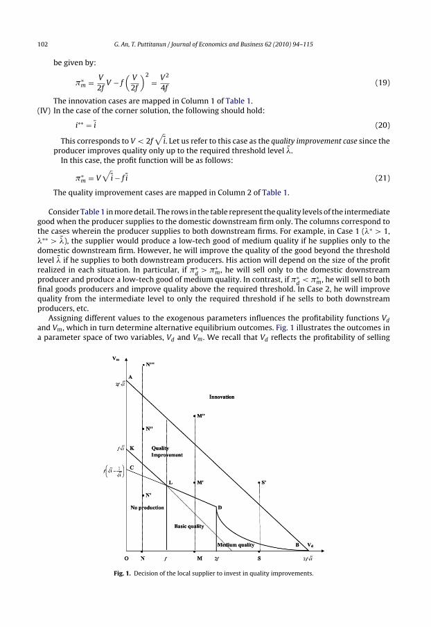
Assigning different values to the exogenous parameters influences the profitability functions Vdand Vm, which in turn determine alternative equilibrium outcomes. Fig. 1 illustrates the outcomes ina parameter space of two variables, Vd and Vm. We recall that Vd reflects the profitability of selling
Fig. 1. Decision of the local supplier to invest in quality improvements.
G. An, T. Puttitanun / Journal of Economics and Business 62 (2010) 94–115 103
to the domestic downstream producer, while Vm reflects the profitability of supplying to the MNE.First, consider the situation wherein the producer supplies to both downstream firms and decides toinnovate. The following conditions should hold:
i∗∗ > i; �∗m > �∗
d; �∗m > 0 (22)
The first inequality in (22) implies that it is profitable to improve quality beyond the required level� by investing more effort than i. The second one indicates that the producer will earn higher profits bysupplying to both downstream producers, rather than to the domestic firm only. And the last conditionis the individual rationality constraint—the producer must earn non-negative profits. Substituting fori**, �m, and �d yields an equivalent set of conditions:
Vd + Vm > 2f√
i
(Vd + Vm)2
4f>
⎧⎪⎪⎨⎪⎪⎩
V2d
4fVd ∈ [2f ; 2f
√i]
Vd − f Vd ∈ [f ; 2f ]0
(23)
The solution to these inequalities corresponds to the area above line AB in Fig. 1.In the region above line AB, the producer will improve quality beyond the threshold level � by
innovating. In this case, it is not the quality requirements but rather the demand for the high-techintermediate good that triggers investment in quality improvements.
Now, consider the case wherein the upstream producer will improve quality only up to thresholdlevel �. The following conditions need to hold:
i∗∗ ≤ i; �∗m > �∗
d; �∗m > 0 (24)
Substituting for i**, �m, and �d yields an equivalent set of conditions
Vd + Vm ≤ 2f√
i (25)
The solution to inequality (25) corresponds to the area below line AB in Fig. 1. Inequalities (26) and(26′) are satisfied above boundaries DB and LD, respectively, and the area that satisfies constraint (27)is above the line KL.16 Therefore, the region ABDLK supports the quality improvement case. In contrast tothe innovation case, in this situation, not only the additional demand but also the quality requirementsfrom the MNE are important in the decision to improve quality. Without those requirements, the localsupplier would produce a good of lower quality.
16 The lines KL and LD intersect at point L, which satisfies: Vd = f. It is obtained by solving: f
√i − Vd ≥ −Vd
(1 − 1√
i
)+
f
(√i − 1√
i
). The corresponding values for Vm at points L and D are f (
√i − 1) and f√
i(√
i − 1)2
, respectively. See Appendix
B for derivations.
104 G. An, T. Puttitanun / Journal of Economics and Business 62 (2010) 94–115
In the case where the upstream producer decides to supply to the domestic downstream produceronly, the following conditions will hold: �∗
m < �∗d
and �∗d
> 0. This is equivalent to
Vm <
⎧⎪⎪⎪⎪⎨⎪⎪⎪⎪⎩
V2d
4f√
i− Vd + f
√i Vd ∈ [2f ; 2f
√i]
−Vd
(1 − 1√
i
)+ f
(√i − 1√
i
)Vd ∈ [f ; 2f ]
. (28)
Vd > f
The region that satisfies these inequalities is given by fLDB in Fig. 1.In the region OKLf, there is no production of either intermediate goods—both are imported. In
addition, the potential demand from the MNE is not large enough to make production of intermediatesprofitable.
Now, consider how different parameter values influence the equilibrium outcome. First, the sizeof the regions in Fig. 1 depends on the investment cost parameter f and the required quality level� (or, equivalently, the effort level i necessary to achieve �). Higher values of effort cost f will moveall the boundaries proportionally in the northeast direction, making ‘no production’ and low-qualityregions larger, which means higher profitability is necessary to induce the producer to invest in quality.Analogously, a higher threshold quality level (higher i) will move boundaries KLDB and AB in theupward direction, again increasing the range of ‘no production’ and the low-quality regions. Otherparameters influence the position of the outcome in the graph. In particular, the intermediates contentin domestic production, ˛, the price of the domestic final good, Pd, the cut-off price, pL , and the marginalcost of producing the intermediate good, c, determine the value of Vd. Therefore, they will determinethe position of the firm in the horizontal dimension of the graph. Analogously, the intermediate’scontent in the MNE production, ˇ, the price of the MNE’s final good, Pm, and the cut-off price, pH ,determine the value of Vm and, therefore, the position of the firm in the vertical dimension. AppendixC shows that a lower marginal cost, c, higher final goods prices, Pd and Pm, higher intermediate goodscut-off prices pL and pH , and higher intermediates content increase the profits of the upstream producerand generate more quality improvements and innovation.
3. The role of the MNE
We will next consider the impact of the MNE’s presence on the host country. Prior to the entryof the MNE into the host country, the position of the local supplier is somewhere on the horizontalaxis (Vm = 0) in Fig. 1. For example, point S corresponds to high profits relative to fixed costs, point Mcorresponds to lower profits, and point N—to a case wherein intermediates are not produced becausefixed costs f are larger than the revenue Vd. The presence of the MNE creates additional demand, whichresults in additional profits (Vm > 0) if the local supplier complies with the required quality standards.This will move points S, M, and N in the upward direction. The extent of the movement depends onthe value of Vm, which in turn is a function of the exogenous parameters. Consider the effects of amultinational’s entry in different initial situations. At point S, the innovation costs are low relative tothe profits earned. The position corresponds to the production of a medium-quality good. This casemight be associated with a large supplier that possesses adequate knowledge of quality-improvingtechnology. However, due to low demand, it is not profitable to invest heavily in quality. This producerwill easily comply with the quality standards when the demand for intermediates rises. He will alsoinnovate more. If the industry is originally at point M, the profits are lower, and the investmentcosts are higher than at point S. This case might be associated with a more competitive intermediateindustry. The equilibrium outcome depends on the profits earned from supplying to the MNE. Belowsection LD, those additional profits are not large enough to induce the upstream producer to investmore in quality. Thus, he will continue to produce basic-quality intermediates. At point M′, theupstream producer will improve quality only up to the threshold level, while a larger increase inprofits (point M′′) induces innovation. Points S′ and M′ ′ in the graph show a backward linkage effect,
G. An, T. Puttitanun / Journal of Economics and Business 62 (2010) 94–115 105
i.e., expansion of the upstream industry due to the presence of the MNE in the downstream industry.In turn, the MNE production level also increases due to the use of higher quality intermediates,i.e., a forward linkage effect. The benefits that are spilled over to the domestic downstream industryconstitute the externality created by the presence of the MNE.
Consider point N on the graph. It originally corresponds to a ‘no production’ region. This positioncan be associated with an underdeveloped country with relatively high investment costs. At point N′,the demand for intermediates from the MNE is not enough to commence production in the upstreamindustry since costs are still high relative to revenue earned. Therefore, at point N′, the presence ofa multinational firm does not have any positive impact on the economy. However, higher demandfor intermediate inputs from the MNE may not only commence the intermediate industry (point N′′)but also induce local suppliers to innovate (point N′′′). This case is consistent with empirical studiesfrom East Asia. Spillovers are present everywhere above section KLDB because the MNE is not able toextract all of the gains from quality improvements in the local economy.
To see how the profit of the domestic downstream producer will change with improvements inthe quality of intermediates, substitute the expressions for intermediates demand and price into theprofit function (2):
∏d
=
⎧⎪⎨⎪⎩
1 − ˛
˛�i
(˛
c
)˛/(1−˛)P1/(1−˛)
dif c/˛ < pL
1 − ˛
˛�iP
1/(1−˛)d
(pL)−˛/(1−˛)
if pL < c/˛
. (29)
As (29) shows, the profit of the domestic final producer will rise with an increase in the quality ofintermediate inputs. As described above, this effect constitutes the externality from the presence ofthe MNE to the domestic final producer. If the local supplier sells to both final producers, his profit isa function of quality as well.
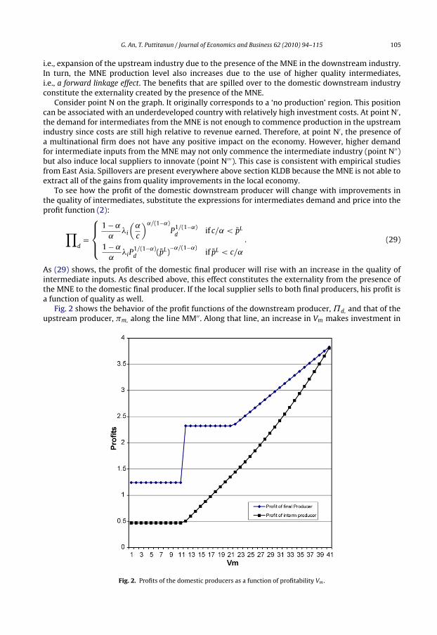
Fig. 2 shows the behavior of the profit functions of the downstream producer, ˘d, and that of theupstream producer, �m, along the line MM′′. Along that line, an increase in Vm makes investment in
Fig. 2. Profits of the domestic producers as a function of profitability Vm .
106 G. An, T. Puttitanun / Journal of Economics and Business 62 (2010) 94–115
quality a more attractive option. The regime switch from the basic to the required quality and towardthe innovation case occurs along the line in an upward direction.
As the figure reveals, profits are constant in the ‘basic-quality’ region (approximately pt. 1–12)until Vm hits the boundary with the ‘quality improvement’ region. At that point, the profits of thedownstream producer jump due to the change in quality of the intermediates, and then stay the samein the ‘quality improvement’ region (approximately pt. 12–21) until Vm hits another boundary withthe ‘innovation’ region. From there on, it is an increasing function of the profitability Vm, since thequality of the intermediate goods will continue to improve. The profit of the intermediate producer islinearly increasing in Vm in the ‘quality improvement’ region and is a convex function in the ‘innovationregion,’ where the highest gains are realized.
Analogously, the MNE profit function can be expressed in terms of the quality level:
∏m
=
⎧⎪⎪⎨⎪⎪⎩
1 − ˇ
ˇ�i
(ˇ
c
)ˇ/(1−ˇ)
P1/(1−ˇ)m if c/ˇ < pH
1 − ˇ
ˇ�iP
1/(1−ˇ)m (pH)
−ˇ/(1−ˇ)if pH < c/ˇ
. (30)
The MNE also gains from the higher quality of intermediate goods.Consumer surplus does not change since the final goods’ prices are given and the demand for high-
tech goods does not yet exist. However, if wages are increasing with employment, then improvementsin the quality of the intermediate good can lead to the expansion of upstream and downstream indus-tries and benefit both skilled and unskilled labor, especially when the presence of the MNE commencesthe upstream industry.17
4. Conclusion
This paper explores how quality standards imposed by the subsidiaries of multinational enterpriseson local suppliers can trigger the adoption of better techniques and processes in local intermedi-ate goods industries, thereby increasing the technological capability of the host country. The modelincludes the possibility that local suppliers might improve product quality beyond the required thresh-old, a situation described in the case studies of East Asia and Japan.
The model shows that the decision to invest in quality improvements depends on the profitabilityof the venture, which in turn is a function of exogenous parameters. In particular, higher prices forfinal goods, high intermediate content in final goods production, as well as lower costs of productionand investment promote quality improvements. If a host country is underdeveloped, which impliesrelatively high costs for quality improvement, the presence of multinational firms might not bringany significant changes to the economy.18 Since the focus of the study is to explore a novel channelfor technological externalities from FDI in developing countries, we do not incorporate the welfareof global consumers in the model. In addition, we limit our analysis to cases when foreign directinvestment is undertaken by multinationals in search of low production costs rather than local demandfor their good.
17 Another aspect not captured in this model is the extent of substitution between the good produced by the domestic producerand the good produced by the MNE. In the event that the expansion of MNE production crowds out domestic production, thewelfare effects of FDI are ambiguous since the profit of domestic producers and the demand for local intermediates mightdecrease. In fact, Aitken and Harrison (1991) examined the Venezuelan manufacturing industry between 1976 and 1989and concluded that the effect of FDI on the productivity of upstream local firms is generally negative. MNEs divert demandfrom domestic to imported inputs, which means that the local suppliers are not able to benefit from potential economies ofscale.
18 In this case, government (and/or MNE) assistance in form of subsidies and technical and educational support might improvethe situation. However, the reader is reminded that the benefits of subsidies should be weighed against the deadweightloss of taxation. In addition, subsidies provided by local governments might not result in the welfare improvement of globalconsumers.
G. An, T. Puttitanun / Journal of Economics and Business 62 (2010) 94–115 107
Appendix A.
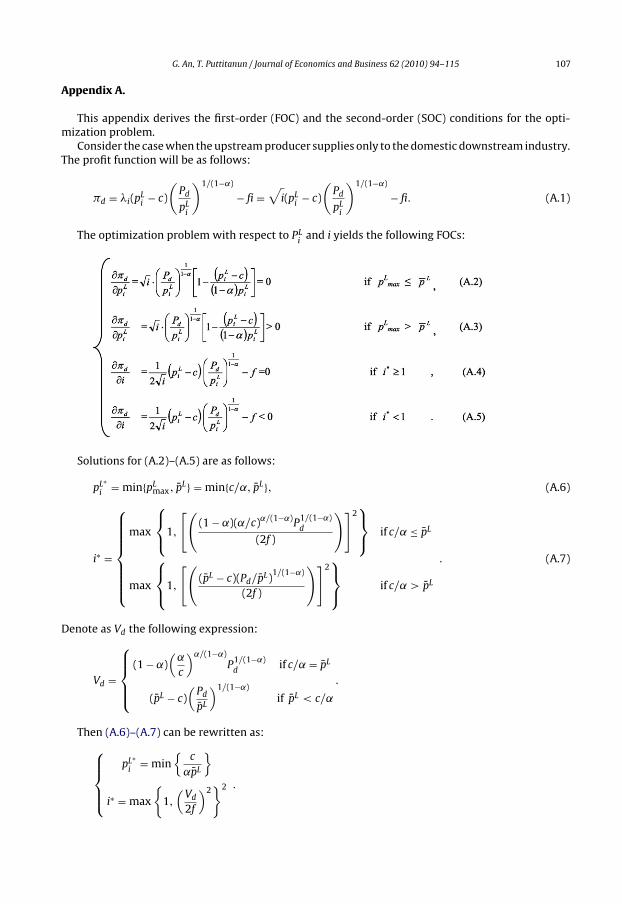
This appendix derives the first-order (FOC) and the second-order (SOC) conditions for the opti-mization problem.
Consider the case when the upstream producer supplies only to the domestic downstream industry.The profit function will be as follows:
�d = �i(pLi − c)
(Pd
pLi
)1/(1−˛)
− fi =√
i(pLi − c)
(Pd
pLi
)1/(1−˛)
− fi. (A.1)
The optimization problem with respect to PLi
and i yields the following FOCs:
Solutions for (A.2)–(A.5) are as follows:
pL∗i = min{pL
max, pL} = min{c/˛, pL}, (A.6)
i∗ =
⎧⎪⎪⎪⎪⎪⎪⎨⎪⎪⎪⎪⎪⎪⎩
max
⎧⎨⎩1,
[((1 − ˛)(˛/c)˛/(1−˛)P1/(1−˛)
d
(2f )
)]2⎫⎬⎭ if c/˛ ≤ pL
max
⎧⎨⎩1,
[((pL − c)(Pd/pL)
1/(1−˛)
(2f )
)]2⎫⎬⎭ if c/˛ > pL
. (A.7)
Denote as Vd the following expression:
Vd =
⎧⎪⎪⎨⎪⎪⎩
(1 − ˛)(
˛
c
)˛/(1−˛)P1/(1−˛)
dif c/˛ = pL
(pL − c)(
Pd
pL
)1/(1−˛)if pL < c/˛
.
Then (A.6)–(A.7) can be rewritten as:⎧⎪⎪⎨⎪⎪⎩
pL∗i
= min{
c
˛pL
}
i∗ = max
{1,(
Vd
2f
)2}2 .
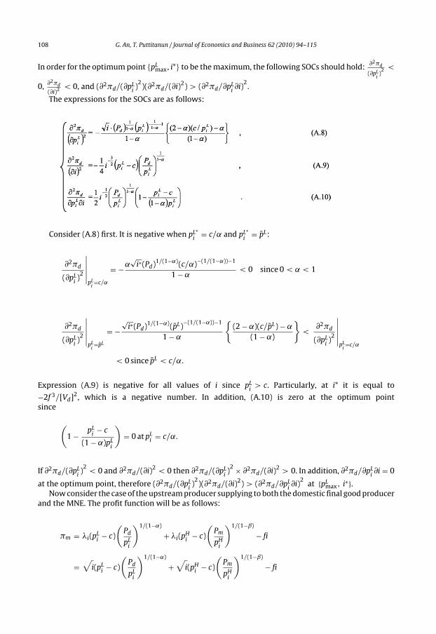
108 G. An, T. Puttitanun / Journal of Economics and Business 62 (2010) 94–115
In order for the optimum point {pLmax, i*} to be the maximum, the following SOCs should hold: ∂2�d
(∂pLi)2 <
0, ∂2�d
(∂i)2 < 0, and (∂2�d/(∂pLi)2)(∂2�d/(∂i)2) > (∂2�d/∂pL
i∂i)
2.
The expressions for the SOCs are as follows:
Consider (A.8) first. It is negative when pL∗i
= c/˛ and pL∗i
= pL:
∂2�d
(∂pLi)2
∣∣∣∣∣pL
i=c/˛
= −˛√
i∗(Pd)1/(1−˛)(c/˛)−(1/(1−˛))−1
1 − ˛< 0 since 0 < ˛ < 1
∂2�d
(∂pLi)2
∣∣∣∣∣pL
i=pL
= −√
i∗(Pd)1/(1−˛)(pL)−(1/(1−˛))−1
1 − ˛
{(2 − ˛)(c/pL) − ˛
(1 − ˛)
}<
∂2�d
(∂pLi)2
∣∣∣∣∣pL
i=c/˛
< 0 since pL < c/˛.
Expression (A.9) is negative for all values of i since pLi
> c. Particularly, at i* it is equal to
−2f 3/[Vd]2, which is a negative number. In addition, (A.10) is zero at the optimum pointsince
(1 − pL
i− c
(1 − ˛)pLi
)= 0 at pL
i = c/˛.
If ∂2�d/(∂pLi)2
< 0 and ∂2�d/(∂i)2 < 0 then ∂2�d/(∂pLi)2 × ∂2�d/(∂i)2 > 0. In addition, ∂2�d/∂pL
i∂i = 0
at the optimum point, therefore (∂2�d/(∂pLi)2)(∂2�d/(∂i)2) > (∂2�d/∂pL
i∂i)
2at {pL
max, i∗}.Now consider the case of the upstream producer supplying to both the domestic final good producer
and the MNE. The profit function will be as follows:
�m = �i(pLi − c)
(Pd
pLi
)1/(1−˛)
+ �i(pHi − c)
(Pm
pHi
)1/(1−ˇ)
− fi
=√
i(pLi − c)
(Pd
pLi
)1/(1−˛)
+√
i(pHi − c)
(Pm
pHi
)1/(1−ˇ)
− fi
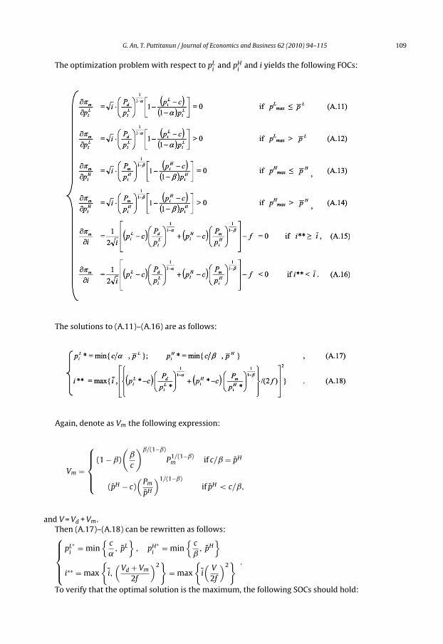
G. An, T. Puttitanun / Journal of Economics and Business 62 (2010) 94–115 109
The optimization problem with respect to pLi
and pHi
and i yields the following FOCs:
The solutions to (A.11)–(A.16) are as follows:
Again, denote as Vm the following expression:
Vm =
⎧⎪⎪⎨⎪⎪⎩
(1 − ˇ)
(ˇ
c
)ˇ/(1−ˇ)
P1/(1−ˇ)m if c/ˇ = pH
(pH − c)(
Pm
pH
)1/(1−ˇ)if pH < c/ˇ,
and V = Vd + Vm.Then (A.17)–(A.18) can be rewritten as follows:⎧⎪⎪⎨⎪⎪⎩
pL∗i
= min{
c
˛, pL
}, pH∗
i= min
{c
ˇ, pH
}i∗∗ = max
{i,(
Vd + Vm
2f
)2}
= max
{i(
V
2f
)2} .
To verify that the optimal solution is the maximum, the following SOCs should hold:
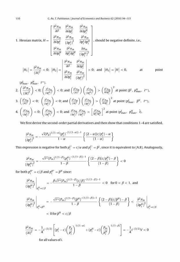
110 G. An, T. Puttitanun / Journal of Economics and Business 62 (2010) 94–115
1. Hessian matrix, H =
⎡⎢⎢⎢⎢⎢⎢⎢⎣
∂2�m
∂i2∂2�m
∂i∂pLi
∂2�m
∂i∂pHi
∂2�m
∂i∂pLi
∂2�m
(∂pLi)2
∂2�m
∂pLi∂pH
i
∂2�m
∂i∂pHi
∂2�m
∂pLi∂pH
i
∂�m
(∂pHi
)2
⎤⎥⎥⎥⎥⎥⎥⎥⎦
, should be negative definite, i.e.,
∣∣H1
∣∣ = ∂2�m
(∂i)2< 0;
∣∣H2
∣∣ =
∣∣∣∣∣∣∣∣∣
∂2�m
∂i2∂2�m
∂i∂pLi
∂2�m
∂i∂pLi
∂2�m
(∂pLi)2
∣∣∣∣∣∣∣∣∣> 0; and
∣∣H3
∣∣ =∣∣H∣∣ < 0, at point
{pLmax, pH
max, i∗∗}.
2.
(∂2�m
(∂i)2
)< 0;
(∂2�m
(∂pHi
)2
)< 0; and
(∂2�m
(∂i)2
)(∂2�m
(∂pHi
)2
)>(
∂2�m
∂i∂pHi
)2at point {pL, pH
max, i∗∗},
3.(
∂2�m
(∂i)2
)< 0;
(∂2�m
(∂pLi)2
)< 0; and
(∂2�m
(∂i)2
)(∂2�m
(∂pLi)2
)>(
∂2�m
∂i∂pLi
)2at point {pL
max, pH, i∗∗},
4.
(∂2�m
(∂pLi)2
)< 0;
(∂2�m
(∂pHi
)2
)< 0; and ∂2�m
(∂pLi)2
∂2�m
(∂pHi
)2 >
[∂2�m
∂pLi∂pH
i
]2at point {pL
max, pHmax, i}.
We first derive the second-order partial derivatives and then show that conditions 1–4 are satisfied.
∂2�m
(∂pLi)2
= −√
i(Pd)1/(1−˛)(pLi)−(1/(1−˛))−1
1 − ˛
{(2 − ˛)(c/pL
i) − ˛
(1 − ˛)
}
This expression is negative for both pL∗i
= c/˛ and pL∗i
= pL , since it is equivalent to (A.8). Analogously,
∂2�m
(∂pHi
)2
= −√
i∗∗(Pm)1/(1−ˇ)(pHi
)−(1/(1−ˇ))−1
1 − ˇ
{(2 − ˇ)(c/pH
i) − ˇ
(1 − ˇ)
}< 0
for both pH∗i
= c/ˇ and pH∗i
= pH since:
∂2�m
(∂pHi
)2
∣∣∣∣∣pH
i=c/ˇ
= −ˇ√
i∗∗(Pm)1/(1−ˇ)(c/ˇ)−(1/(1−ˇ))−1
1 − ˇ< 0 for 0 < ˇ < 1, and
∂2�m
(∂pHi
)2
∣∣∣∣∣pH
i=pH
= −√
i∗∗(Pm)1/(1−ˇ)(pH)−(1/(1−ˇ))−1
1 − ˇ
{(2 − ˇ)(c/pH) − ˇ
(1 − ˇ)
}<
∂2�m
(∂pHi
)2
∣∣∣∣∣pH
i=c/ˇ
< 0 for pH < c/ˇ
∂2�m
(∂i)2= −1
4i−(3/2)
[(pL
i − c)
(Pd
pLi
)1/(1−˛)
+ (pHi − c)
(Pm
pHi
)1/(1−ˇ)]
= −14
i−(3/2)V < 0
for all values of i.
G. An, T. Puttitanun / Journal of Economics and Business 62 (2010) 94–115 111
Particularly, at i**, ∂2�m/(∂i)2 = −2f 3/[V ]2 < 0∂2�m/∂pL
i∂pH
i= 0 for all values of pL
iand pH
i .
∂2�m
∂pLi∂i
= 1
2√
i
(Pd
pLi
)1/(1−˛) [1 − (pL
i− c)
(1 − ˛)pLi
]
∂2�m
∂pHi
∂i= 1
2√
i
(Pm
pHi
)1/(1−ˇ) [1 − (pH
i− c)
(1 − ˇ)pHi
]
Consider point {pLmax, pH
max, i∗∗} first.
∂2�m
∂pLi∂i
= f
V
(Pd
pLmax
)1/(1−˛) [1 − (pL
max − c)(1 − ˛)pL
max
]= 0
∂2�m
∂pHi
∂i= f
V
(Pm
pHmax
)1/(1−ˇ) [1 − (pH
max − c)(1 − ˇ)pH
max
]
This yields the following Hessian matrix:
H =
⎡⎢⎢⎢⎢⎢⎢⎣
−2f 3
V20 0
0−˛V(Pd)1/(1−˛)(c/˛)(˛−2)/(1−˛)
2f (1 − ˛)0
0 0−ˇV(Pm)1/(1−ˇ)(c/ˇ)(ˇ−2)/(1−ˇ)
2f (1 − ˇ)
⎤⎥⎥⎥⎥⎥⎥⎦
∣∣H1
∣∣ = −2f 3
[V ]2< 0
∣∣H2
∣∣ = −2f 3
[V ]2
−˛V(Pd)1/(1−˛)(c/˛)(˛−2)/(1−˛)
2f (1 − ˛)> 0
∣∣H3
∣∣ = −2f 3
[V ]2
−˛V(Pd)1/(1−˛)(c/˛)(˛−2)/(1−˛)
2f (1 − ˛)−ˇV(Pm)1/(1−ˇ)(c/ˇ)(ˇ−2)/(1−ˇ)
2f (1 − ˇ)< 0
→ H is negative definite at point {pLmax, pH
max, i∗∗}, therefore {pLmax, pH
max, i∗∗} is the maximum.Consider point {pL, pH
max, i∗∗} next.
∂2�m
(∂pHi
)2
∂2�m
(∂i)2= −ˇV(Pm)1/(1−ˇ)(c/ˇ)(ˇ−2)/(1−ˇ)
2f (1 − ˇ)−2f 3
[V ]2> 0
[∂2�m
∂pHi
∂i
]2
={
f
V
(Pm
pHmax
)1/(1−ˇ) [1 − (pH
max − c)(1 − ˇ)pH
max
]}2
= 0 since
(1 − pH
max − c
(1 − ˛)pHmax
)= 0
∴ ∂2�m
(∂pHi
)2
∂2�m
(∂i)2>
[∂2�m
∂pHi
∂i
]2

112 G. An, T. Puttitanun / Journal of Economics and Business 62 (2010) 94–115
Analogously, at point {pLmax, pH, i∗∗}:
∂2�m
(∂pLi)2
∂2�m
(∂i)2= −˛V(Pd)1/(1−˛)(c/˛)(˛−2)/(1−˛)
2f (1 − ˛)−2f 3
[V ]2> 0
[∂2�m
∂pLi∂i
]2
={
f
V
(Pd
pLmax
)1/(1−˛) [1 − (pL
max − c)(1 − ˛)pL
max
]}2
= 0 since
(1 − pL
max − c
(1 − ˛)pLmax
)= 0
∴ ∂2�m
(∂pLi)2
∂2�m
(∂i)2>
[∂2�m
∂pLi∂i
]2
.
Finally, at point {pLmax, pH
max, i}:
∂2�m
(∂pLi)2
∂2�m
(∂pHi
)2
= −˛√
i(Pd)1/(1−˛)(c/˛)−(1/(1−˛))−1
1 − ˛
−ˇ√
i(Pm)1/(1−ˇ)(c/ˇ)(ˇ−2)/(1−ˇ)
1 − ˇ> 0
[∂2�m
∂pLi∂pH
i
]2
= 0
∴ ∂2�m
(∂pLi)2
∂2�m
(∂pHi
)2
>
[∂2�m
∂pLi∂pH
i
]2
That proves that the optimal solution is the maximum.
Appendix B.
Point D is an intersection of lines LD and DB.
LD : Vm = −Vd
(1 − 1√
i
)+ f
(√i − 1√
i
)(B.1)
DB : Vm = V2d
4f√
i− Vd + f
√i (B.2)
Since they intersect at point Vd = 2f, substitute this value into either (B.1) or (B.2):
(B.1) : Vm = −2f
(1 − 1√
i
)+ f
(√i − 1√
i
)= f√
i[−2
√i + 1 + i] = f√
i[1 −
√i]
2,
(B.2) : Vm = 4f 2
4f√
i− 2f + f
√i = f√
i[−2
√i + 1 + i] = f√
i[1 −
√i]
2.
Analogously, point L is an intersection of lines KL and LD.
KL : Vm = f√
i − Vd (B.3)
LD : Vm = −Vd
(1 − 1√
i
)+ f
(√i − 1√
i
)(B.4)
G. An, T. Puttitanun / Journal of Economics and Business 62 (2010) 94–115 113
Since they intersect at point Vd = f, substitute this value into either (B.3) or (B.4).
(B.3) : Vm = f√
i − f = f (√
i − 1)
(B.4) : Vm = −f
(1 − 1√
i
)+ f
(√i − 1√
i
)= f (
√i − 1)
Appendix C.
This appendix shows a comparative static exercise for the variables Vd and Vm. Recall that
Vd =
⎧⎪⎪⎨⎪⎪⎩
(1 − ˛)(
˛
c
)˛/(1−˛)Pd
1/(1−˛) if c/˛ < pL
(pL − c)(
Pd
pL
)1/(1−˛)if pL < c/˛
,
therefore,
∂Vd
∂c=
⎧⎪⎪⎨⎪⎪⎩
−(
˛Pd
c
)1/(1−˛)< 0 if c/˛ < pL
−(
Pd
pL
)1/(1−˛)< 0 if pL < c/˛
(C.1)
∂Vd
∂Pd=
⎧⎪⎪⎨⎪⎪⎩(
˛Pd
c
)˛/(1−˛)> 0 if c/˛ < pL
(pL − c)(1 − ˛)
(Pd)˛/1−˛
pL 1/1−˛> 0 if pL < c/˛
, (C.2)
∂Vd
∂pL=
⎧⎨⎩
0 if c/˛ < pL(Pd
pL
)1/(1−˛)(
c − ˛pL
pL(1 − ˛)
)> 0 if pL < c/˛
(C.3)
Expressions (C.1)–(C.3) imply that a lower marginal cost of production, c, a higher price for the domesticfinal good, Pd (which can result from industry protection or higher demand), as well as a higher cut-off price, pL , increase the profits of the intermediate goods producer and raise the desire to invest inquality (a rightward movement in the graph).
Analogously, recall from (17) that
Vm =
⎧⎪⎪⎨⎪⎪⎩
(1 − ˇ)
(ˇ
c
)ˇ/(1−ˇ)
Pm1/(1−ˇ) if c/ˇ < pH
(pH − c)(
Pm
pH
)1/(1−ˇ)if pH < c/ˇ
.
Hence,
∂Vm
∂c=
⎧⎪⎪⎨⎪⎪⎩
−(
ˇPm
c
)1/(1−ˇ)
< 0 if c/ˇ < pH
−(
Pm
pH
)1/(1−ˇ)< 0 if pH < c/ˇ
, (C.4)
114 G. An, T. Puttitanun / Journal of Economics and Business 62 (2010) 94–115
∂Vm
∂Pm=
⎧⎪⎪⎪⎨⎪⎪⎪⎩
(ˇPm
c
)ˇ/(1−ˇ)
> 0 if c/ˇ < pH
(pH − c)(1 − ˇ)
(Pm)ˇ/1−ˇ
pH 1/1−ˇ> 0 if pH < c/ˇ
, (C.5)
∂Vm
∂pH=
⎧⎨⎩
0 if c/ˇ < pH(Pm
pH
)1/(1−ˇ)(
c − ˇpH
pH(1 − ˇ)
)> 0 if pH < c/ˇ
, (C.6)
∂Vm
∂ˇ=
⎧⎪⎪⎪⎨⎪⎪⎪⎩
(Pm)1/(1−ˇ)
(1 − ˇ)
(ˇ
c
)ˇ/(1−ˇ)
lnˇPm
c> 0 if c/ˇ < pH
(pH − c)(
Pm
pH
)1/(1−ˇ) 1
(1 − ˇ)2ln
Pm
pH> 0 if pH < c/ˇ
, (C.7)
Equations (C.4)–(C.7) imply that a lower marginal cost, c, a higher price for final good, Pm, a highercontent of intermediates in MNE production, as well as a higher cut-off price, pH , increase profit andtherefore the extent of quality improvements (upward movement).
References
Aghion, P., & Howitt, P. (1998). Endogenous growth theory. Cambridge, MA: MIT Press.Aitken, B., & Harrison, A. (Nov. 1991). Are there spillovers from foreign direct investment? Evidence from panel data for Venezuela.
Mimeo, MIT and the World Bank.Aitken, B., & Harrison, A. (1999). Do domestic firms benefit from direct foreign investment? Evidence from Venezuela. American
Economic Review, 89, 605–618.Baldwin, R. E., Braconier, H., & Forslid, R. (1999) Multinationals, endogenous growth and technological spillovers: Theory and
evidence. Centre for Economic Policy Research Discussion Paper, 2155.Blalock, G. (2001) Technology from Foreign Direct Investment: Strategic Transfer through Supply Chains. Paper presented at the
Empirical Investigations in International Trade Conference at Purdue University, November 9–11, 2001 [Part of doctoralresearch at Haas School of Business, University of California, Berkeley].
Blalock, G., & Gertler, P. J. (2008). Welfare gains from foreign direct investment through technology transfer to local suppliers.Journal of International Economics, 74(2), 402–421.
Brash, D. T. (1966). American investment in Australian industry. Canberra: Australian University Press.Blomström, M., & Kokko, A. (1998). Multinational corporations and spillovers. Journal of Economic Surveys, 12(3), 247–277.Blomström, M., & Persson, H. (1983). Foreign investment and spillover efficiency in an underdeveloped economy: Evidence
from the Mexican manufacturing industry. World Development, 11(6), 493–501.Blomström, M., & Wolff, E. (1994). Multinational corporations and productivity convergence in Mexico. In W. Baumol, R. Nelson,
& E. Wolff (Eds.), Convergence of productivity: Cross-national studies and historical evidence (pp. 243–259). New York: OxfordUniversity Press.
Caves, R. (1974). Multinational firms, competition and productivity in host-country markets. Economica, 41, 176–193.Caves, R. (1996). Multinational Enterprise and Economic Analysis. Cambridge: Cambridge University Press.Chuang, Y., & Lin, C. (1999). Foreign direct investment, R&D and spillover efficiency: Evidence from Taiwan’s manufacturing
firms. Journal of Development Studies, 35, 117–137.Das, S. (1987). Externalities, and technology transfers through multinational corporations: A theoretical analysis. Journal of
International Economics, 22, 171–182.Djankov, S., & Hoekman, B. (2000). Foreign investment and productivity growth in Czech enterprises. World Bank Economic
Review, 14, 49–64.Findlay, R. (1978). Relative backwardness, direct foreign investment, and the transfer of technology: A simple dynamic model.
Quarterly Journal of Economics, 92, 1–16.Fosfuri, A., Motta, M., & Ronde, T. (2001). Foreign direct investment and spillovers through workers’ mobility. Journal of Inter-
national Economics, 53, 205–222.Görg, H., & Strobl, E. (2001). Multinational companies and productivity spillovers: A meta-analysis. The Economic Journal, 111,
723–739.Haddad, M., & Harrison, A. (1993). Are there positive spillovers from direct foreign investment? Evidence from panel data for
Morocco. Journal of Development Economics, 42, 51–74.Haskel, J. E., Pereira, S. C., and Slaughter, M. J. (2002) Does Inward Foreign Direct Investment Boost the Productivity of Domestic
Firms? National Bureau of Economic Research (Cambridge, MA). Working Paper No. 8724.Henson, S., & Mitullah, W. (2004) Kenyan exports of Nile perch: Impact of food safety standards on an export-oriented supply
chain. The World Bank Policy Research Working Paper 3349 (World Bank).Hobday, M. (1995). Innovation in East Asia: The challenge to Japan. London: Aldershot.Jaffee, S., & Henson, S. (2004) Standards and agro-food exports from developing countries: Rebalancing the debate. The World
Bank Policy Research Working Paper Series 3348 (World Bank).
G. An, T. Puttitanun / Journal of Economics and Business 62 (2010) 94–115 115
Katz, J. M. (1969). Production functions, foreign investment and growth. North Holland: Amsterdam.Katz, J. M. (1987). Technology generation in Latin American manufacturing industries. New York: St. Martin’s Press.Keller, W., & Yeaple, S. (2003) Multinational enterprises, international trade and productivity growth: Firm-level evidence from
the U.S. CEPR Discussion Papers 3805.Kokko, A. (1994). Technology, market characteristics, and spillovers. Journal of Development Economics, 43, 279–293.Kokko, A. (1996). Productivity spillovers from competition between local firms and foreign affiliates. Journal of International
Development, 8, 517–530.Lall, S. (1980). Vertical interfirm linkages in LDCs: An empirical study. Oxford Bulletin of Economics and Statistics, 42, 203–226.Lall, S. (2000). Technological change and industrialization in the Asian newly industrializing economies: Achievements and
challenges. In L. Kim, & R. R. Nelson (Eds.), Technology, learning, & innovation (pp. 13–68). Cambridge: Cambridge UniversityPress.
Mansfield, E., & Romeo, A. (1980). Technology transfer to overseas subsidiaries by U.S.-based firms. Quarterly Journal of Economics,95(4), 737–750.
Markusen, J. R. (2001). Intellectual property rights, and multinational investment in developing countries. Journal of InternationalEconomics, 53, 189–204.
Markusen, R. J., & Venables, A. J. (1999). Foreign direct investment as a catalyst for industrial development. European EconomicReview, 43(2), 335–356.
Maskus, K. E., Otsuki, T., & Wilson, J. S. (2001). An empirical framework for analyzing technical regulations and trade. In K. E.Maskus, & J. S. Wilson (Eds.), Quantifying the impact of technical barriers to trade: Can it be done? (pp. 29–57). Ann Arbor:University of Michigan Press.
McAleese, D., & McDonald, D. (1978). Employment growth and development of linkages in foreign-owned and domestic man-ufacturing enterprises. Oxford Bulletin of Economics and Statistics, 40, 321–339.
Moran, T. H. (1998). Foreign direct investment and development: The new policy agenda for developing countries and economies intransition. Washington, DC: Institute for International Economics.
Posner, M. V. (1961) International trade and technical change. Oxford Economic Papers, No. 13, pp. 323–341.Rodriguez-Clare, A. (1996). Multinationals, linkages, and economic development. American Economic Review, 86, 852–873.Schive, C. (1990). The foreign factor: The multinational corporation’s contribution to the economic modernization of the Republic of
China. Stanford, CA: Hoover Institution Press.Schoors, K., & Van der Tol, B. (2002) Foreign direct investment spillovers within and between sectors: Evidence from Hungarian
data. Working Papers of Faculty of Economics and Business Administration. Belgium: Ghen University.Smarzynska, B. K. (2004). Does foreign direct investment increase the productivity of domestic firms? In search of spillovers
through backward linkages. American Economic Review, 94(3), 605–627.Stanford, L. (2002). Constructing “quality”: The political economy of standards in Mexico’s avocado industry. Agriculture and
Human Values, 19(4), 293–310.Temple, J. (1999). The new growth evidence. Journal of Economic Literature, 37, 112–156.Vernon, R. (1966). International investment and international trade in the product cycle. Quarterly Journal of Economics, 82(2),
190–207.Watanabe, S. (1983). Technical cooperation between large and small firms in the Filipino automobile industry. In S. Watanabe
(Ed.), Technology marketing and industrialization: Linkages between small and large enterprises (pp. 97–131). New Delhi:Macmillan.