HAL Id: hal-00578550https://hal.archives-ouvertes.fr/hal-00578550v3

Submitted on 19 Mar 2012

HAL is a multi-disciplinary open accessarchive for the deposit and dissemination of sci-entific research documents, whether they are pub-lished or not. The documents may come fromteaching and research institutions in France orabroad, or from public or private research centers.

L’archive ouverte pluridisciplinaire HAL, estdestinée au dépôt et à la diffusion de documentsscientifiques de niveau recherche, publiés ou non,émanant des établissements d’enseignement et derecherche français ou étrangers, des laboratoirespublics ou privés.

Quantile-based optimization of Noisy ComputerExperiments with Tunable Precision

Victor Picheny, David Ginsbourger, Yann Richet, Grégory Caplin

To cite this version:Victor Picheny, David Ginsbourger, Yann Richet, Grégory Caplin. Quantile-based optimization ofNoisy Computer Experiments with Tunable Precision. 2012. <hal-00578550v3>

Quantile-Based Optimization of Noisy

Computer Experiments with Tunable

Precision

Victor Picheny

CERFACS42 Avenue Gaspard Coriolis, 31057 Toulouse, France

phone: +33 (0)5 61 19 30 99; email: picheny@cerfacs.frDavid Ginsbourger

Departement of Mathematics and Statistics, University of BernAlpeneggstrasse 22, 3012 Bern, Switzerland

phone: +41 (0)31 631 54 62; email: david.ginbourger@stat.unibe.ch

Yann RichetInstitut de Radioprotection et de Surete Nucleaire

31 avenue de la Division Leclerc, 92260 Fontenay-aux-Roses, Francephone: +33 (0)1 58 35 88 84;email: yann.richet@irsn.fr

Gregory CaplinInstitut de Radioprotection et de Surete Nucleaire

31 avenue de la Division Leclerc, 92260 Fontenay-aux-Roses, Francephone: +33 (0)1 58 35 90 08; email: gregory.caplin@irsn.fr

Abstract

This article addresses the issue of kriging-based optimization of stochastic simula-tors. Many of these simulators depend on factors that tune the level of precision ofthe response, the gain in accuracy being at a price of computational time. The con-tribution of this work is two-fold: firstly, we propose a quantile-based criterion for thesequential design of experiments, in the fashion of the classical Expected Improvementcriterion, which allows an elegant treatment of heterogeneous response precisions. Sec-ondly, we present a procedure for the allocation of the computational time given to eachmeasurement, allowing a better distribution of the computational effort and increasedefficiency. Finally, the optimization method is applied to an original application innuclear criticality safety. This article has supplementary material online.

Keywords: Kriging, Expected Improvement, stochastic simulators.technometrics tex template (do not remove)

1

1. INTRODUCTION

Using metamodels for facilitating optimization and statistical analysis of computationally

expensive simulators has become commonplace. In particular, the kriging-based Efficient

Global Optimization (EGO) algorithm (Jones, Schonlau and Welch 1998) has been recog-

nized as an efficient tool for deterministic black-box optimization.

The way a simulator response follows the function of interest is called fidelity. Oftentimes,

a large range of response fidelities is available by tuning factors that control the complexity

of numerical methods. For instance, the precision of a finite element analysis can be con-

trolled by the discretization technique or the solver convergence. When the response stems

from Monte Carlo methods (which are often referred to as stochastic simulators), accuracy

(measured by the inverse of the response variance) is proportional to sample size. Such

simulators are often called noisy simulators, since they return approximate solutions that

depart from the exact value by an error term that can be considered as a random quantity.

In an optimization context, having noise in the responses requires a proper adaptation of

criteria and algorithms. Furthermore, for each simulation run, the user has to set a trade-off

between computational cost and response precision. This additional degree of freedom may

greatly improve the efficiency of the optimization, but requires appropriate tools to choose

this trade-off and the ability to work with heterogeneous precisions.

Using metamodels for noisy optimization has been addressed by several authors. Huang,

Allen, Notz and Zeng (2006) and Forrester, Keane and Bressloff (2006) proposed kriging-

based strategies for optimization of uniformly noisy functions. However, little work can

be found in the case of heterogeneous noise. Most approaches combining optimization and

variable precision are found in the multifidelity framework (Forrester, Sobester and Keane

2007; Gano, Renaud, Martin and Simpson 2006), but consider only two fidelity levels, the

low-fidelity model being used as a helping tool to choose the high-fidelity evaluations.

This article proposes two contributions to this framework. First, we define an extension

of EI based on quantiles that enables an elegant treatment of both continuous or discrete

fidelities. The proposed criterion not only depends on the noise variances from the past, but

also on the fidelity of the new candidate measurement. Second, we study a procedure taking

advantage of the possibility to choose the fidelity level at each iteration.

In the next section, we define the “noisy” framework we are considering and present briefly

2

the kriging model. Section 3 describes the classical kriging-based optimization procedure,

and its limitation with noisy functions. In Section 4, we propose a new infill criterion, called

Expected Quantile Improvement (EQI), well-suited for the noisy framework, and in Section

5 we propose a numerical trick for tuning one of the EQI parameters to account for finite

computational budgets. Section 6 describes a procedure for on-line decision on precision

level. Finally, this procedure is compared to existing kriging-based methods, and applied to

an original application in nuclear criticality safety.

2. NOTATIONS AND CONCEPTS

2.1 The noisy optimization problem

We consider a single objective, unconstrained minimization problem over a compact set D.

The deterministic objective function y : x ∈ D ⊂ Rd −→ y(x) ∈ R is here observed with

noise, that is, the user only has access to measurements of the form yi = y(xi) + ǫi, where ǫi

is assumed to be one realization of a “noise” random variable ε. In the rest of this article,

we make the assumption that the observation noises are normally distributed, centered and

independent from one run to each other: εi ∼ N (0, τ 2i ) independently.

2.2 Noise in computer experiments

In classical experiments, noise usually accounts for a large number of uncontrolled variables

(variations of the experimental setup, measurement precision, etc.). In computer experi-

ments, noise can have many sources, including modeling and discretization error, incomplete

convergence, and finite sample size for Monte-Carlo methods, see for instance Forrester,

Keane and Bressloff (2006) or Gramacy and Lee (2010a) for a detailed discussion.

The nature of the noise depends on the associated simulator. When classical Monte-

Carlo simulations are involved in the output evaluation, error is independent from one run

to each other, even for measurements with the same input variables. Such simulators are

often referred to as stochastic, and are the main target for the method presented here. The

industrial application described in Section 7.2 belongs to this category.

Errors due to a simplification of the physics, geometry, or meshing, tend to show strong

correlations, especially for simulations with similar fidelities, and repeated experiments pro-

vide the same observations. This situation has been addressed in the multi-fidelity literature

3

(see Kennedy and O’Hagan (2000) and Qian and Wu (2008) for modeling, Forrester et al.

(2007) and Huang et al. (2006) for optimization) and is not considered here, although many

of the concepts presented here may apply with a proper adaptation of the kriging model.

Error due to incomplete convergence can be either treated as correlated noise or not. In

Forrester, Bressloff and Keane (2006), it is observed that simulations tend to converge in

unison, which makes the partial convergence equivalent to a multi-fidelity problem. How-

ever, when the output convergence behavior varies substantially across the design space, the

hypothesis of independence of the error between runs may become reasonable, especially if

experiments are well spread in the design space and different convergence levels are used.

2.3 Experiments with tunable precision

As mentioned in the introduction, the precision of many simulators can be tuned by the

user, for instance by changing the number of solver steps for incomplete convergence or the

sample size for Monte-Carlo methods. Here, we consider that, for every measurement, the

noise variance τ 2i = τ(ti) is a monotonically decreasing function of computation time ti.

A perhaps “canonical” example of tunable precision is when the response considered is

obtained by averaging an arbitrary number bi of independent drawings (which is a typical

situation in the framework of robust optimization for instance):

Yi =1

bi

bi∑

j=1

y(xi) + εi,j, (1)

when εi,j ∼ N (0, ν2). We have then Yi ∼ N(y(xi),

ν2

bi

), so τ 2(t) = ρν2/t, ρ being the time

needed for a single drawing. The value of bi chosen by the user tunes the precision of Yi.

In this work, we make two strong assumptions: (a) the computation time, and hence the

error variance, is controllable, and (b) the function τ(t) is accurately known. Although some

stochastic simulators, such as the one described in Section 7.2, directly provide an accurate

estimate of the output uncertainty, in most real applications a learning study is necessary,

typically assuming a (simple) parametric form for the variance. In the case of Monte-Carlo

simulators and assuming small variations of the output across the design space, we have

τ 2(t) = C/t, where C is an unknown constant which can be estimated when building the

kriging model, as described in Section 2.4.

4

Finally, for simulators relying on Monte Carlo or on iterative solvers, the response cor-

responding to a given precision is not obtained directly but more as a limit of intermediate

responses of lower precisions. For each measurement, the noisy response yi is thus obtained

as last term of a sequence of measurements yi[1], . . . , yi[bi], where bi ∈ N is the number of

calculation steps at the ith measurement.

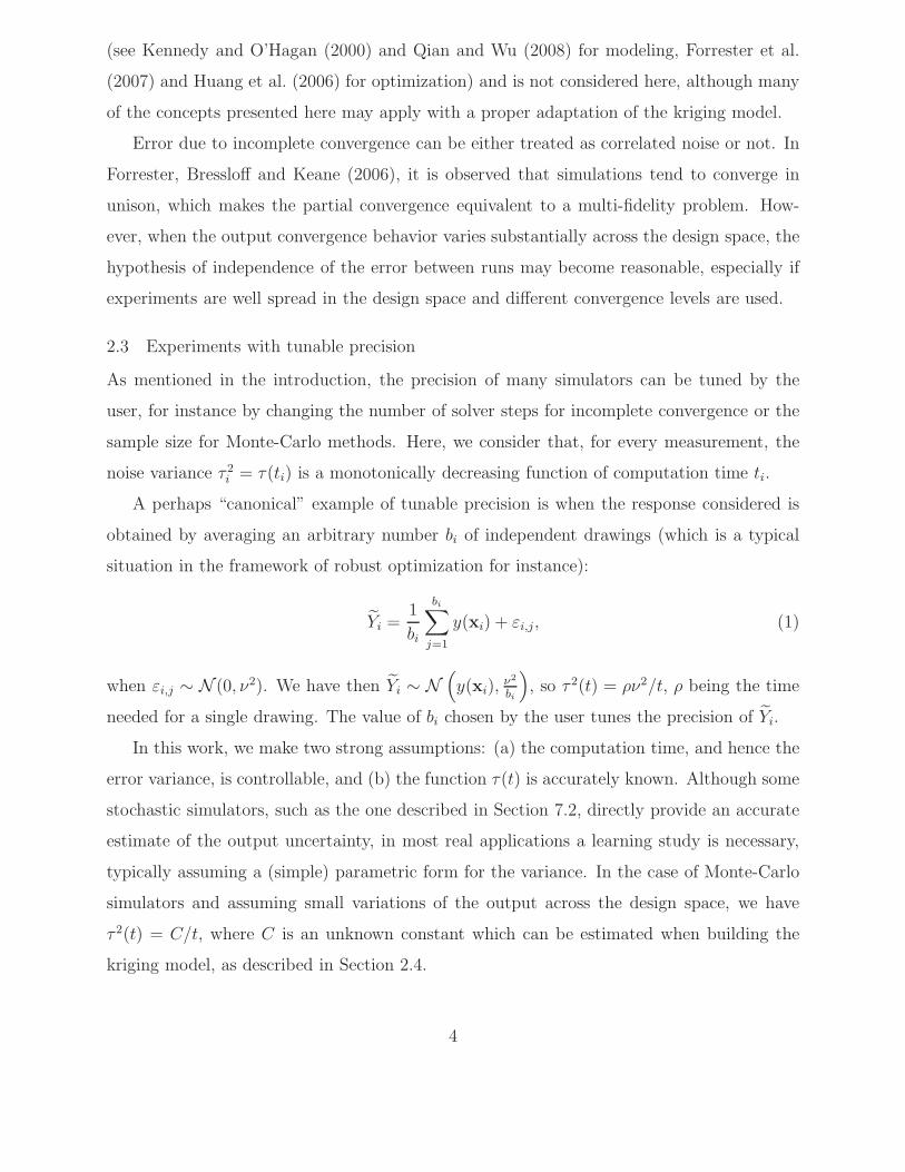
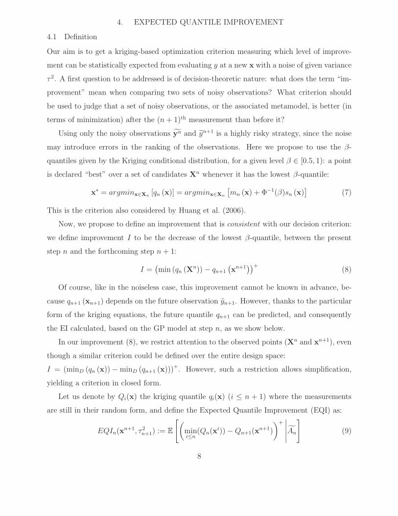
Figure 1 represents two examples of response convergence. First, the convergence of the

output of the stochastic simulator of Section 7.2 is drawn for its nominal design values. Here,

the variance is known accurately, and depicted by the 95% confidence interval. The curve

ytilde represents the sequence y[j], j = 1 . . . 100. The second figure is taken from Forrester,

Bressloff and Keane (2006) and represents the convergence of an objective function (namely

the L/D ratio) calculated using an Euler simulation of an aerofoil, as a function of the number

of solver steps. The response oscillates around its final value with decreasing amplitude.

Here, error variance is not available directly and requires the specification of and inferences

for a parametric model for τ based on a couple of trial responses such as this one.

0 20 40 60 80 100

−0.55

−0.5

−0.45

−0.4

Time increments

y

90%CI

Figure 1: Examples of tunable precision responses. Left: convergence of the output of

MORET for its nominal design values; right: partially converged response of a CFD code.

2.4 The Kriging metamodel

In this work, we use a (generalized) Gaussian Process regression model (as in Rasmussen and

Williams (2006), chapter 2), where y is assumed to be one realization of a random process

Y with an unknown constant trend µ ∈ R, and a stationary covariance kernel k, i.e. of the

form k : (x,x′) ∈ D2 −→ k(x,x′) = σ2r(x − x′;ψ) for some admissible correlation function

5

r with parameters ψ. Provided that the process Y and the Gaussian measurement errors

εi are stochastically independent and that the error variances are given, the distribution of

Y (x) conditional on the event An = {Y (xi) + εi = yi, 1 ≤ i ≤ n} is:

Y (x)|An ∼ N (mn(x), s2n(x)) (2)

where mn(.) and s2n(.) are respectively the kriging mean and variance, given by:

mn(x) = µn + kn(x)T (Kn + ∆n)−1(yn − µn1n), (3)

s2n(x) = σ2 − kn(x)T (Kn + ∆n)−1kn(x) +

(1 − 1T

n (Kn + ∆n)−1kn(x))2

1Tn (Kn + ∆n)−11n

, (4)

with σ2 = k(x,x), yn = (y1, . . . , yn)T ,Kn = (k(xi,xj))1≤i,j≤n, kn(x) = (k(x,x1), . . . , k(x,xn))T ,

∆n is a diagonal matrix of diagonal terms τ 21 . . . τ

2n , 1n is a n × 1 vector of ones, and

µn = 1Tn (Kn + ∆n)−1yn/1T

n (Kn + ∆n)−11n is the best linear unbiased estimate of µ.

As for a classical kriging model, the covariance parameters σ2 and ψ usually need to

be estimated, using maximum likelihood (ML) for instance and considering the noise vari-

ances as known. If the noise variances are not known but a simple parametric functional

relashionship is assumed between the τ 2i ’s and the ti’s, the corresponding parameters may be

embedded within the ML procedure. For instance, assuming a Monte-Carlo-type behavior

of the form τ 2i = C/ti, the likelihood would depend on C through ∆n and µn.

3. KRIGING-BASED OPTIMIZATION; LIMITATIONS WITH NOISY FUNCTIONS

The EGO algorithm (Jones et al. 1998) builds a sequential design with the goal of finding a

global minimum of a black-box function. It consists in sequentially evaluating y at a point

maximizing a figure of merit relying on Kriging, the Expected Improvement criterion (EI),

and updating the metamodel after each new observation.

In the noiseless case, with yi = y(xi) (1 ≤ i ≤ n), yn = (y1, . . . , yn)T , Xn = {x1, . . . ,xn}and An denoting the event Y (Xn) = yn, the improvement provided by sampling at x is

defined by I = max (0,min (Y (Xn)) − Y (x)), and the EI is its expectation given by the GP

model:

EIn(x) := E[(min(Y (Xn)) − Y (x))+ |An

]= E

[(min(yn) − Y (x))+ |An

](5)

6

An integration by parts yields the well-known analytical expression:

EIn(x) := (min(yn) −mn(x)) Φ

(min(yn) −mn(x)

sn(x)

)+ sn(x)φ

(min(yn) −mn(x)

sn(x)

), (6)

where Φ and φ are respectively the cumulative distribution function and the probability

density function of the standard Gaussian law. The latter analytical expression is very con-

venient since it allows fast evaluations of EI, and even analytical calculation of its gradient.

Now, in the context of noisy evaluations, (5) is not very satisfactory for at least two

reasons. Firstly, the current minimum min(Y (Xn)) is not deterministically known condi-

tionally on the noisy observations, unlike the noiseless case. Secondly, the EI is based on the

improvement produced by a deterministic evaluation of y at the candidate point x. Now, if

the next evaluation is noisy, Y (x) will remain inexactly known. It would hence benefit from

a new criterion taking the precision of the next measurement into account.

In Huang et al. (2006), a heuristic modification of the EI called Augmented Expected

Improvement (AEI) is proposed for uniformly noisy observations. The mean predictor at

the training point with smallest kriging quantile is used as a surrogate value for min(Y (Xn)),

and the EI is multiplied by a penalization function 1 − τ√s2n(x)+τ2

to limit replications.

A more rigorous alternative, as noted in Gramacy and Lee (2010b) and Gramacy and Pol-

son (2011), consists of computing the EI based on the joint distribution of (min(Y (Xn)), Y (x))

conditional on An; however, in this form the EI must be estimated by expensive Monte-Carlo

simulations, which makes the EI maximization challenging.

Finally, the Integrated Expected Conditional Improvement (IECI), proposed in Gramacy

and Lee (2010b), evaluates by how much a candidate measurement at a given point would

affect the expected improvement over the design space, thereby naturally taking past and

future noises into account. However, this criterion requires a numerical integration over the

design space, which can be time-consuming, especially in high dimensions.

The next section presents a class of criteria (indexed by a parameter β tuning a quantile

level) that takes into account past and future noises with transparent probabilistic foun-

dations, and which can be derived analytically as a function of the future point and its

associated noise level.

7

4. EXPECTED QUANTILE IMPROVEMENT

4.1 Definition

Our aim is to get a kriging-based optimization criterion measuring which level of improve-

ment can be statistically expected from evaluating y at a new x with a noise of given variance

τ 2. A first question to be addressed is of decision-theoretic nature: what does the term “im-

provement” mean when comparing two sets of noisy observations? What criterion should

be used to judge that a set of noisy observations, or the associated metamodel, is better (in

terms of minimization) after the (n+ 1)th measurement than before it?

Using only the noisy observations yn and yn+1 is a highly risky strategy, since the noise

may introduce errors in the ranking of the observations. Here we propose to use the β-

quantiles given by the Kriging conditional distribution, for a given level β ∈ [0.5, 1): a point

is declared “best” over a set of candidates Xn whenever it has the lowest β-quantile:

x∗ = argminx∈Xn[qn (x)] = argminx∈Xn

[mn (x) + Φ−1(β)sn (x)

](7)

This is the criterion also considered by Huang et al. (2006).

Now, we propose to define an improvement that is consistent with our decision criterion:

we define improvement I to be the decrease of the lowest β-quantile, between the present

step n and the forthcoming step n+ 1:

I =(min (qn (Xn)) − qn+1

(xn+1

))+(8)

Of course, like in the noiseless case, this improvement cannot be known in advance, be-

cause qn+1 (xn+1) depends on the future observation yn+1. However, thanks to the particular

form of the kriging equations, the future quantile qn+1 can be predicted, and consequently

the EI calculated, based on the GP model at step n, as we show below.

In our improvement (8), we restrict attention to the observed points (Xn and xn+1), even

though a similar criterion could be defined over the entire design space:

I = (minD (qn (x)) − minD (qn+1 (x)))+. However, such a restriction allows simplification,

yielding a criterion in closed form.

Let us denote by Qi(x) the kriging quantile qi(x) (i ≤ n + 1) where the measurements

are still in their random form, and define the Expected Quantile Improvement (EQI) as:

EQIn(xn+1, τ 2n+1) := E

[(mini≤n

(Qn(xi)) −Qn+1(xn+1)

)+∣∣∣∣∣An

](9)

8

where the dependence on the future noise τ 2n+1 appears through Qn+1(x)’s distribution.

The randomness of Qn+1(x) conditional on An is indeed a consequence from Yn+1 :=

Y (xn+1) + εn+1 having not been observed yet at step n. However, following the fact that

Yn+1|An is Gaussian with known mean and variance, one can show that Qn+1(.) is a GP

conditional on An (see proof and details in appendix). Furthermore, mini≤n(Qn(xi)) is

known conditional on An. As a result, the proposed EQI is analytically tractable, and we

get by a similar calculation as in (6):

EQIn(xn+1, τ 2n+1) =

(min(qn) −mQn+1

)Φ

(min(qn) −mQn+1

sQn+1

)+sQn+1φ

(min(qn) −mQn+1

sQn+1

)

(10)

where qn := {qn(xi), i ≤ n} is the set of current quantile values at the already visited points,

mQn+1 := E[Qn+1(xn+1)|An] is Qn+1(x

n+1)’s conditional expectation —seen from step n, and

s2Qn+1

:= V ar[Qn+1(xn+1)|An] is its conditional variance, both derived in appendix.

4.2 Properties

The EQI criterion has the following important properties:

- in absence of future noise (τ 2n+1 = 0), the future quantile at xn+1 coincides with the

observation yn+1 = y(xn+1); it follows directly that Qn+1(xn+1)|An = Yn+1|An, so the EQI

is equal to the classical EI with a plugin of the kriging quantiles for min(yn)

- in absence of past noise (for the n first observations), min(qn) is equal to the minimum

of the observations, min(yn)

- in absence of both past and future noise, the EQI is then equal to the classical EI.

The parameter β tunes the level of reliability wanted on the final result (which plays

a similar role as the power parameter of the generalized improvement of Schonlau, Welch

and Jones (1998)). With β = 0.5, the design points are compared based on the kriging

mean predictor only, without taking into account the prediction variance at those points,

while high values of β (i.e. near to 1) penalize designs with high uncertainty, which is a

more conservative approach. Hence, with a high β, the criterion is more likely to favor

observation repetitions or clustering, in order to locally decrease the prediction variance,

while with β = 0.5, the criterion can be expected to be more exploratory.

The future noise τ 2n+1 also strongly affects the shape of the EQI. Indeed, a very noisy

future observation can only have a very limited influence on the kriging model. Then, the

9

only way to get a non-zero improvement is either to sample where qn(x) is minimum if this

point is not in Xn (the lowest quantile will then be chosen on the set Xn+1 instead of Xn,

which will bring an improvement even if qn+1 = qn), or to sample at the current best point,

which may decrease its uncertainty and brings a small but measurable improvement. On the

contrary, if τ 2n+1 is very small, the EQI behaves like the classical EI, making the well-known

trade-off between exploration and exploitation.

Figure 2 illustrates the dependence of the EQI on both τ 2n+1 and β. The actual function

is y(x) = 12

(sin(20x)

1+x+ 3x3cos(5x) + 10(x− 0.5)2 − 0.6

), the initial design consists of five

equally-spaced measurements, with noise variances equal to 0.02.

0 0.1 0.2 0.3 0.4 0.5 0.6 0.7 0.8 0.9 1−2

−1

0

1

2Kriging and actual function

ym

K

+/− 2*sK

ytilde

0 0.1 0.2 0.3 0.4 0.5 0.6 0.7 0.8 0.9 10

0.1

EQI with β = 0.9

τ2=1

τ2=0.1

τ2=0.01

0 0.1 0.2 0.3 0.4 0.5 0.6 0.7 0.8 0.9 10

0.05

0.1

EQI with β = 0.5

Figure 2: Actual function, kriging, and corresponding EQI for three future noise levels and

two quantile levels. The bars of the upper graph show the noise amplitude (±2 × τi).

We can see that the choice of the future noise level has a substantial influence on the

criterion. With small noise variance, the EQI behaves like the classical EI, with highest values

in regions with high uncertainty and low mean predictions. With higher noise variances and

high quantiles, the criterion becomes very conservative since is it high only in the vicinity

of existing measurements. With β = 0.5, the EQI is high even for the largest variance.

10

However, here five curves out of six return similar optimal locations (i.e. x near 0.4 or 0.6),

which indicates that the influence of τ and β may not be critical during the first optimization

steps.

4.3 EQI as a function of computational time

EQI measures the effect of a new measurement with variance τ 2n+1, while we defined in Section

2 a measurement at location xi as depending on a computational time ti. In our framework

of tunable precision, two cases have to be distinguished. Let tn+1 be the computational time

used at iteration n+ 1. At unsampled locations, the EQI criterion is simply evaluated with

τ 2n+1 = τ 2(tn+1). At existing observations, a different value has to be used; if not, the EQI

would estimate the value of a new measurement with variance τ 2(tn+1), instead of estimating

the value of improving the existing measurement. To compute this value, we use the fact

that it is equivalent for the kriging model to have several measurements at the same point

with independent noises or a single equivalent measurement which is the weighted average

of the observations (see supplementary material for proof). For instance, let yi,1 and yi,2 be

two measurements with noise levels τ 2i,1 and τ 2

i,2 respectively. They are equivalent to

yi,eq =τ−2i,1 yi,1 + τ−2

i,2 yi,2

τ−2i,1 + τ−2

i,2

, (11)

with variance τ 2i,eq the harmonic mean of τ 2

i,1 and τ 2i,2, namely:

1

τ 2i,eq

:=1

τ 2i,1

+1

τ 2i,2

=⇒ τ 2i,eq =

τ 2i,1τ

2i,2

τ 2i,1 + τ 2

i,2

. (12)

Now, we want to measure the effect of improving a measurement with initial error variance

τ 2(ti) until the variance τ 2(ti + tn+1) is reached. This is equivalent, in terms of the kriging

model, to taking a new measurement with noise variance:

τ 2(ti → ti + tn+1) :=τ 2(ti)τ

2(ti + tn+1)

τ 2(ti) − τ 2(ti + tn+1). (13)

This formula is obtained from (12), with τ 2i,eq = τ 2(ti + tn+1), τ

2i,1 = τ 2(ti) and τ 2

i,2 = τ 2(ti →ti + tn+1). Hence, at xi, EQI may be evaluated with τ 2

n+1 = τ 2(ti → ti + tn+1).

The next section proposes a numerical trick for tuning tn+1 to account for finite compu-

tational budgets.

11

5. OPTIMIZATION WITH FINITE COMPUTATIONAL BUDGET

It is well-known that the EGO algorithm is a so-called myopic strategy, since its criterion EI

always considers the next step as if it were the last one. However, for most computer exper-

iments, the total computational budget is bounded, and prescribed by industrial constraints

such as time and power limitations. In the deterministic framework, this results in a limited

(given) number of observations for optimization. It has been shown (Mockus (1988) followed

by Ginsbourger and Le Riche (2010)) that taking into account the finite budget may modify

the optimization strategy and improve significantly its efficiency.

Here, the concept of finite budget is particularly critical, since each observation requires a

trade-off between accuracy and rapidity, and in general, the user has to trade off between the

total number of observations and their precision. In linear modeling, this problem is typical

of the theory of optimal designs (Fedorov and Hackl 1997), with the notable difference that

we face it here within a sequential strategy, and a non-linear (kriging) model.

The computational constraint implies that the sum of all computational times is fixed to a

given budget, say T0. At step n, the remaining budget for optimization is Tn+1 = T0−∑n

i=1 ti.

The EQI criterion allows taking into account such computational budget in the choice of

the new candidate observations. Indeed, the future noise level τ 2n+1, which is a parameter of

EQI, will stand here for the finite budget. Given a computational budget Tn+1, the smallest

noise variance achievable (i.e. the largest precision) for a new measurement is τ 2(Tn+1),

and τ 2(ti → ti + Tn+1) at xi (1 ≤ i ≤ n), assuming that all the remaining budget will be

attributed to this measurement. Note that in the course of the optimization process, the

remaining budget decreases, so τ 2 (Tn+1) (respectively τ 2(ti → ti + Tn+1)) increases with n.

Then, we propose to set τ 2n+1 = τ 2(Tn+1) (resp. τ 2(ti → ti+Tn+1)) for the EQI calculation,

meaning that the EQI will measure the potential improvement if all the remaining budget

would be attributed to the next observation. Of course, the actual budget tn+1 for the next

observation may be a lot smaller than Tn+1 so the optimization does not stop after one step.

With this setting, the new experiment is chosen knowing that even if all the budget was used

for a single observation, its noise variance would not decrease below a certain value.

Consequently, the EQI will behave differently at the beginning and at the end of the

optimization. When the budget is high, EQI will tendencially be higher in unexplored

regions, since it is where accurate measurements are likely to be most efficient (the EQI will

12

actually be almost similar to a classical EI). At the end of the optimization, however, when

the remaining time is small, the EQI will be small in unexplored regions since even if the

actual function is low, there is not enough computational time to obtain a lower quantile

than the current best one. In that case, the EQI will be highest close to or at the current

best point(s) and favor local search.

6. ALLOCATION OF RESOURCE

This section proposes two algorithmic schemes based on EQI. First, the baseline approach

is described, where a fixed time is allocated at each iteration; then, a strategy is proposed

to take advantage of the response convergence monitoring to dynamically adapt the budget

to each measurement.

6.1 Constant allocation

First, we assume that the computational budget T0 can be divided in elementary time steps

te, so that T0 = N × te. An elementary step can correspond to a given number of solver

iterations for partial convergence, or to a number of drawings for stochastic simulators. An

algorithm with constant allocation will then proceed to attribute each of the N elementary

time steps to either generate new measurements or improve accuracy on existing ones.

At step n, a budget n × te < T0 as already been spent on the measurements, so Tn+1 =

T0 − n × te. The EQI criterion is maximized over D with τ 2n+1 = τ 2(Tn+1) at unsampled

locations and τ 2n+1 = τ 2(ti → ti +Tn+1) at xi (1 ≤ i ≤ n). Once the new point xn+1 is chosen

and the measurement is made, the kriging model has to be updated, by either adding xn+1

to Xn if xn+1 /∈ Xn or by replacing the previous values of yi[bi] and τ 2i [bi] by yi[bi + 1] and

τ 2i [bi + 1], respectively, in the kriging equations.

The trade-off between precision and number of measurements is here determined by EQI,

depending if it is maximum at a sampled or an unsampled design. Taking the finite budget

into account affects the trade-off, since with large budget it is more exploratory, hence likely

to be maximum at unsampled points, while with small budget it is more likely to be maximal

at existing points (see Figure 2, EQI with β = 0.9 and τ 2 = 0.1 or 0.01).

Note that this procedure allows the (closely related) problem of optimization of a ho-

mogeneously noisy function to be addressed, considering that each observation requires a

13

constant time te, and has a constant noise variance ν2. At each optimization step, the user

has the option of either sampling at a new location or duplicating an existing measurement,

so allocating all the remaining budget to a measurement means performing N − n replica-

tions at this point, hence leading to the situation described in Section 2.3 (equation 1). In

that case, it is straightforward to get τ 2(ti → ti + Tn+1) = ν2

N−n= τ 2(Tn+1), so the crite-

rion is written similarly at sampled and unsampled locations. Thus, in this framework, the

procedure simplifies to maximizing at each step EQIn(., ν2

N−n).

6.2 On-line allocation

The constant allocation strategy of the previous section performs N − n0 EGO iterations,

and each requires the running of an inner optimization loop for the maximization of the

EQI, which can be very time-consuming. Hence, the elementary time step te must be chosen

to be large enough to limit the number of EQI optimizations (otherwise choosing the next

measurement could take more time than performing it!). Typically, with partial convergence

or stochastic simulators, te must be chosen to be much larger than a single solver iteration

or drawing, respectively. This limitation can greatly hinder the flexibility and potential of

tunable precision, since it reduces the possibilities of a quasi-continuum of fidelities to a few

discrete precision levels.

Here, we propose a heuristic for dynamically choosing the computational resource given

to an experiment. A simple way to do so is to monitor the evolution of the EQI at the

current observation point. Indeed, instead of maximizing the EQI after each te is spent,

we will choose an observation point, and allocate several time steps on it until a criterion is

met. As for the constant allocation case, the EQI is updated after each step, by replacing the

previous values of response and noise yi[bi] and τ 2i [bi] by yi[bi +1] and τ 2

i [bi +1], respectively,

in the kriging equations, and by replacing the future noise level τ 2(ti → ti + Tn+1) by

τ 2(ti + te → ti + Tn+1 − te).

By construction, the updated EQI tends to decrease when computation time is added,

since (a) the kriging uncertainty reduces at the observation point, and (b) EQI decreases

when τ 2(ti → ti +Tn+1) increases. However, if the measurement converges to a good (small)

value, EQI can increase temporarily. Conversely, if the measurement converges to a high

value, EQI decreases faster. Hence, we can define a (“point switching”) stopping criterion

14

for resource allocation based on EQI. If the EQI decreases below a certain value, carrying on

the calculations is not likely to help the optimization, so the observation process should stop

and another point should be chosen. Here, we propose the interruption of a measurement

and search for a new point when the current value of the EQI is less than a proportion of

the initial EQI value (that is, the value of EQI when starting the measurement process at

that point), for instance 50%.

The sequence of this new procedure is as follows: first, find xn+1 = argmaxx∈D(EQI(x), τ 2(Tn+1)),

store the corresponding value EQI(xn+1), τ 2(Tn+1)) as reference, and then invest elementary

measurements at this point until the EQI with updated data falls under a given proportion

γ ∈]0, 1[ of the reference value. The operation of choosing the most promising point is

then started again, and so on until the total computational budget has been spent. Note

that the final number of measurements and EQI maximizations are not determined before-

hand but adapts automatically to the budget and resource distribution, and may be a lot

smaller than the number of steps N (especially with small γ). The algorithm is presented

in pseudo-code form in Table 1. For conciseness, this algorithm does not consider the case

where xn+1 ∈ Xn, which requires different treatement, as in Section 6.1. In the examples in

Section 7, xn+1 ∈ Xn is considered.

7. EXPERIMENTS

7.1 Comparison to the Augmented Expected Improvement (AEI) procedure

The strategy proposed in Section 6.2 is compared to the AEI method as proposed in Huang

et al. (2006) for the optimization of homogeneously noisy experiments, which has already

been found to be very competitive compared to other local or global optimizers such as the

revised simplex search (Humphrey and Wilson 2000) or DIRECT (Gablonsky and Kelley

2001). Both EQI and AEI heuristics are compared to the classical EI, using a noisy kriging

model (as in Section 2.4) and with the minimal value of the observations replaced by the

minimum of the kriging mean at the observations, which can be considered as the baseline

approach. As test problems, we employed two analytical benchmark problems, the d = 6

dimensional Hartman function (Dixon and Szego 1978) and the d = 5 dimensional Ackley

15

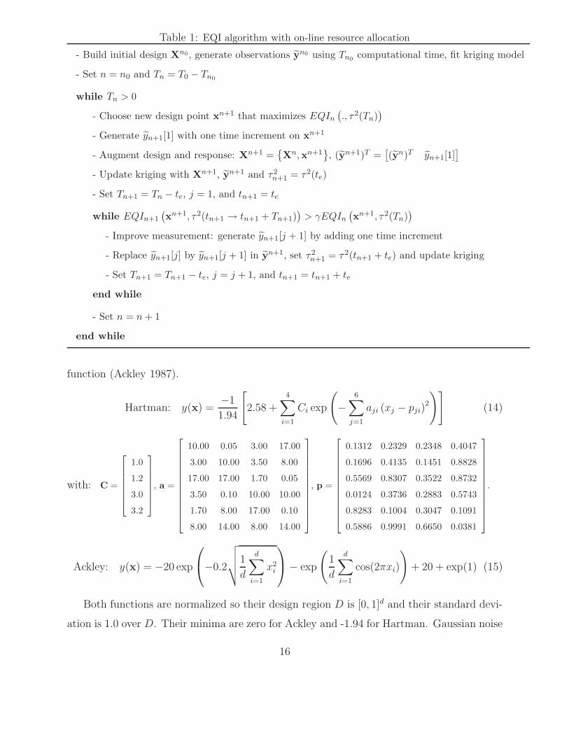
Table 1: EQI algorithm with on-line resource allocation

- Build initial design Xn0, generate observations yn0 using Tn0 computational time, fit kriging model

- Set n = n0 and Tn = T0 − Tn0

while Tn > 0

- Choose new design point xn+1 that maximizes EQIn

(., τ2(Tn)

)

- Generate yn+1[1] with one time increment on xn+1

- Augment design and response: Xn+1 ={Xn,xn+1

}, (yn+1)T =

[(yn)T yn+1[1]

]

- Update kriging with Xn+1, yn+1 and τ2n+1 = τ2(te)

- Set Tn+1 = Tn − te, j = 1, and tn+1 = te

while EQIn+1

(xn+1, τ2(tn+1 → tn+1 + Tn+1)

)> γEQIn

(xn+1, τ2(Tn)

)

- Improve measurement: generate yn+1[j + 1] by adding one time increment

- Replace yn+1[j] by yn+1[j + 1] in yn+1, set τ2n+1 = τ2(tn+1 + te) and update kriging

- Set Tn+1 = Tn+1 − te, j = j + 1, and tn+1 = tn+1 + te

end while

- Set n = n + 1

end while

function (Ackley 1987).

Hartman: y(x) =−1

1.94

[2.58 +

4∑

i=1

Ci exp

(−

6∑

j=1

aji (xj − pji)2

)](14)

with: C =

1.0

1.2

3.0

3.2

, a =

10.00 0.05 3.00 17.00

3.00 10.00 3.50 8.00

17.00 17.00 1.70 0.05

3.50 0.10 10.00 10.00

1.70 8.00 17.00 0.10

8.00 14.00 8.00 14.00

, p =

0.1312 0.2329 0.2348 0.4047

0.1696 0.4135 0.1451 0.8828

0.5569 0.8307 0.3522 0.8732

0.0124 0.3736 0.2883 0.5743

0.8283 0.1004 0.3047 0.1091

0.5886 0.9991 0.6650 0.0381

.

Ackley: y(x) = −20 exp

−0.2

√√√√1

d

d∑

i=1

x2i

− exp

(1

d

d∑

i=1

cos(2πxi)

)+ 20 + exp(1) (15)

Both functions are normalized so their design region D is [0, 1]d and their standard devi-

ation is 1.0 over D. Their minima are zero for Ackley and -1.94 for Hartman. Gaussian noise

16

ǫ ∼ N (0, 10τ 2) is added to the analytical functions. An ordinary kriging model (constant

trend) with Matern 5/2 anisotropic covariance function is used for both functions.

In order to model a tunable fidelity framework while allowing a fair comparison between

methods, each noisy measurement yi is taken as the average of several function evaluations

as described in Section 2.3. For the AEI procedure, which is designed for homoscedastic

noise, ten time steps are used for each observation, so the noise variance is τ 2. For the EQI

procedure, the noise variance potentially varies between 10τ 2 and 10τ 2/T0.

For both methods, the initial design sets are chosen as LHS designs with maximin cri-

terion, and are generated using ten time steps for each observation. The total optimization

budget is chosen to be equal to two times the budget needed to generate the initial design

set. Two versions of EQI are tested, with β = 0.5 (decision based on kriging mean only) and

with β = 0.9; the criteria are referred to as EQI.50 and EQI.90, respectively.

Several budgets, noise levels and initial design sizes are tested. The different configura-

tions are summarized in Table 2. The noise level τ can be compared to objective function

standard deviation (SD), which is one for both functions. With τ = 0.2, the optimization

problem can be considered as very noisy. The total budget is deliberately chosen to be very

small since it may correspond to typical situations in real-life applications.

For each configuration, 40 initial designs and observations are generated to account for

randomness in the LHS designs and the observations. The kriging parameters are estimated

only at the initial step, using the R package DiceKriging (Roustant, Ginsbourger and Deville

2011), so all the methods use the same models. Sequential parameter re-estimation is not

done here (even though it might result in better precision) so the algorithms can be compared

in terms of kriging variance or quantile.

Table 2: Summary of the test problem configurations

Function Initial design size n0 Budget T0 τ

Ackley 25 points 500 steps 0.05

Ackley 50 points 1000 steps 0.2

Hartman 60 points 1200 steps 0.2

The current minimizer forAEI or EQI.90 is x∗ = argmin1≤i≤nqn(xi), and argmin1≤i≤nmn(xi)

for EQI.50 or EI. The optimization performances are compared based on y(x∗) (actual value

17

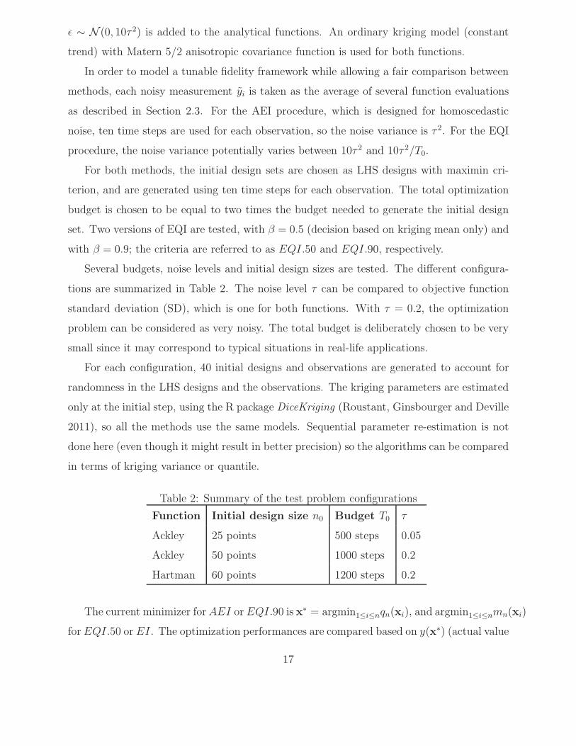
at x∗) and sn(x∗) (kriging SD), which are represented using boxplots on Figure 3.

1)

0

0.5

1

1.5

2

2.5

3

3.5

4

EI AEI EQI50 EQI90

y

0.01

0.02

0.03

0.04

0.05

0.06

0.07

0.08

EI AEI EQI50 EQI90

Kriging SD

2)0.5

1

1.5

2

2.5

3

EI AEI EQI50 EQI90

y

0.03

0.04

0.05

0.06

0.07

0.08

0.09

EI AEI EQI50 EQI90

Kriging SD

3)

−1.9

−1.85

−1.8

−1.75

EI AEI EQI50 EQI90

y

0.03

0.04

0.05

0.06

0.07

0.08

0.09

0.1

0.11

0.12

0.13

EI AEI EQI50 EQI90

Kriging SD

Figure 3: Boxplots of actual value (y) and kriging standard deviation (sn) at x∗ for the

different methods on 1) the Ackley function with τ = 0.05 and 500 steps, 2) the Ackley

function with τ = 0.2 and 1000 steps, 3) the Hartman function τ = 0.2 and 1200 steps.

For the Ackley function, with τ = 0.05, EQI outperforms AEI in terms of actual value and

kriging uncertainty at x∗. The choice of β = 0.5 provides the best results. With τ = 0.2, AEI

provides the best results in terms of optimization (y(x∗)). However, sn(x∗) is significantly

lower for EQI.90 than for the other methods, which illustrates the tendency of this method

to reduce uncertainty at the expense of exploration.

For the Hartman function, EQI slightly outperforms the two other methods in terms of

y(x∗). In terms of kriging uncertainty, EI and AEI are clearly less efficient than EQI. The

18

difference between the strategies β = 0.5 and β = 0.9 appear clearly; indeed, with β = 0.5,

the choice of the best design is made on the kriging mean only; on the other hand, with

β = 0.9, observations with high uncertainty are penalized so that sn(x∗) is always small.

Table 3 shows the average number of distinct measurements and the average number

of time steps at x∗. Even though EI and AEI use uniform allocation, their values are not

constant because some measurements are repeated (i.e. criteria are maximal at existing

measurements during optimization). For instance, the first row and last column of the table

indicates that for EI, there is on average four repeated measurements at x∗.

For the small budget and small noise on the Ackley function, the online allocation of

Section 6.2 resulted with more measurements than for AEI and EI. Here, online allocation

was used to improve exploration by having more measurement locations and resulted in

better performance in terms of y(x∗) (see Figure 3). On the contrary, for the large budget

and large noise, it resulted in accurate measurements at x∗ to the detriment of exploration.

For the Hartman function, the number of measurements is almost equivalent for all methods.

It is interesting to note that for the Ackley function with τ = 0.05 and the Hartman

function, the average number of time steps at x∗ is smaller for EQI than for EI and AEI

but sn(x∗) is also smaller (Figure 3), which is counter-intuitive. For EQI, the small sn(x∗)

is obtained because the measurements form a cluster around x∗.

Table 3: Computational time allocation during optimization

Configuration Nb of distinct measurements Time steps at x∗

(Function, Initial design, Budget, τ) EQI.50 EQI.90 AEI EI EQI.50 EQI.90 AEI EI

Ackley, 25 points, 500 steps, 0.05 76 70 45 44 6 6 43 40

Ackley, 50 points, 1000 steps, 0.2 72 63 87 98 21 64 15 11

Hartman, 60 points, 1200 steps, 0.2 130 118 117 103 5 8 23 38

7.2 Application to a 2D benchmark from nuclear criticality safety assessments

In this section, the optimization algorithm is applied to the problem of safety assessment

of a nuclear system involving fissile materials. The benchmark system used is an interim

storage of dry PuO2 powder into a regular array of storage tubes. The criticality safety

of this system is evaluated through the neutron multiplication factor (called k-effective or

19

keff), which models the nuclear chain reaction trend: keff > 1 implies an increasing neutron

production leading to an uncontrolled chain reaction, and keff < 1 is the safety state required

for fuel storage.

The neutron multiplication factor depends on many parameters such as the composition

of fissile materials, operation conditions, geometry, etc. For a given set of parameters, the

value of keff can be evaluated using the MORET stochastic simulator (Fernex, Heulers,

Jacquet, Miss and Richet 2005), which is based on Markov Chain Monte-Carlo (MCMC)

simulation techniques. The precision of the evaluation depends on the amount of simulated

particles (neutrons), which is tunable by the user.

When assessing the safety of a system, one has to ensure that, given a set of admissible

values D for the parameters x, there are no physical conditions under which the keff can reach

the critical value of one. The search for the worst combination of parameters x defines a noisy

optimization problem which is often challenging in practice, due to the high computational

expense of the simulator. An efficient resolution technique for this problem is particularly

crucial since this optimization may be done numerous times.

In this article, we focus on the maximization of keff with respect to two parameters, the

other possible inputs being fixed to their most penalizing values (based on expert knowledge):

- d.puo2, the powder density, with original range [0.5, 4] g.cm−3, rescaled to [0, 1],

- d.water, the density of water between storage tubes, with range [0, 1], which accounts

for the possible flooding of the storage (leading to an interstitial moderation of the neutrons

interacting from a storage tube to another one).

Hence, to agree with previous notations, we set: x = (d.puo2, d.water), and y(x) =

−keff(x). Simulation time is assumed to be proportional to the number of neutrons simulated

(the entry cost of a new simulation being neglected). Since the simulator is based on Monte-

Carlo, the variance of the keff estimate is exactly inversely proportional to the number of

neutrons. The variance slightly varies with input parameters, but this dependence can be

considered negligible here.

For practical considerations, the optimization space D is discretized in a 75 × 75 grid,

and for each new measurement the EQI maximization is performed by an exhaustive search

on the grid. The incremental time step te is defined by the simulation of 4000 particles,

which takes about half a minute on a 3 GHz CPU. The response noise standard deviation

20

can take values between 5.67 × 10−2 (one time step) and 4.01 × 10−3 (200 time steps).

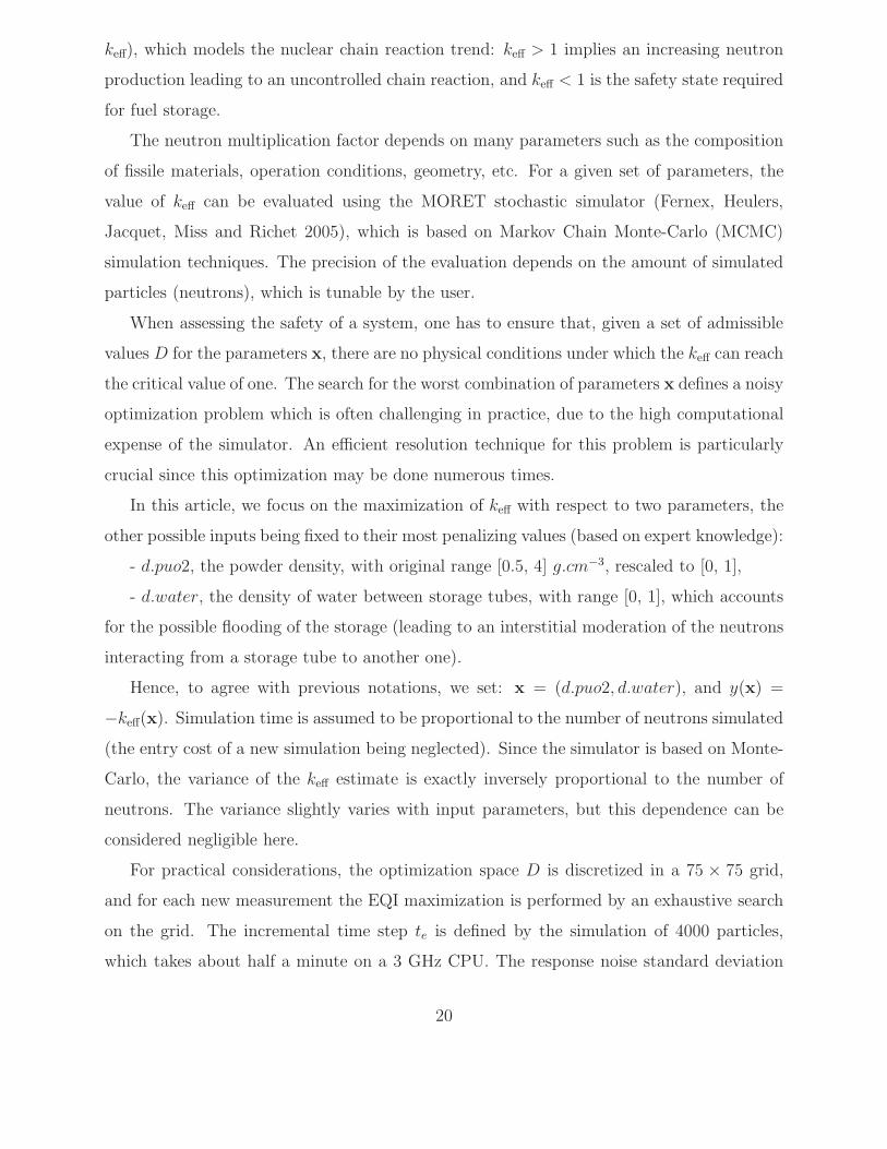
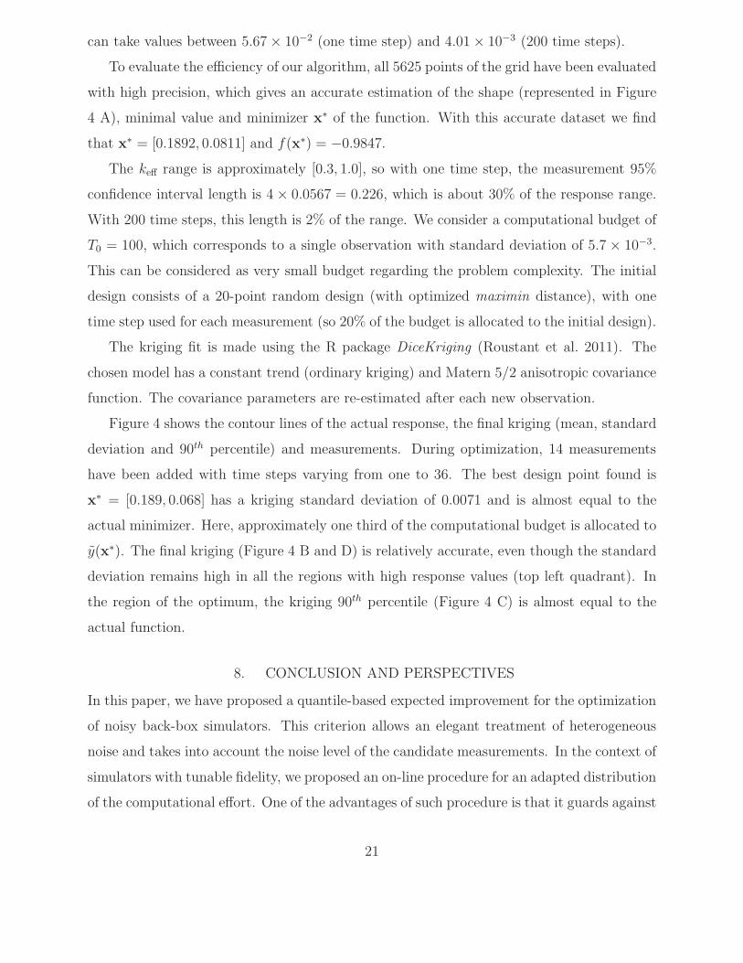
To evaluate the efficiency of our algorithm, all 5625 points of the grid have been evaluated

with high precision, which gives an accurate estimation of the shape (represented in Figure

4 A), minimal value and minimizer x∗ of the function. With this accurate dataset we find

that x∗ = [0.1892, 0.0811] and f(x∗) = −0.9847.

The keff range is approximately [0.3, 1.0], so with one time step, the measurement 95%

confidence interval length is 4 × 0.0567 = 0.226, which is about 30% of the response range.

With 200 time steps, this length is 2% of the range. We consider a computational budget of

T0 = 100, which corresponds to a single observation with standard deviation of 5.7 × 10−3.

This can be considered as very small budget regarding the problem complexity. The initial

design consists of a 20-point random design (with optimized maximin distance), with one

time step used for each measurement (so 20% of the budget is allocated to the initial design).

The kriging fit is made using the R package DiceKriging (Roustant et al. 2011). The

chosen model has a constant trend (ordinary kriging) and Matern 5/2 anisotropic covariance

function. The covariance parameters are re-estimated after each new observation.

Figure 4 shows the contour lines of the actual response, the final kriging (mean, standard

deviation and 90th percentile) and measurements. During optimization, 14 measurements

have been added with time steps varying from one to 36. The best design point found is

x∗ = [0.189, 0.068] has a kriging standard deviation of 0.0071 and is almost equal to the

actual minimizer. Here, approximately one third of the computational budget is allocated to

y(x∗). The final kriging (Figure 4 B and D) is relatively accurate, even though the standard

deviation remains high in all the regions with high response values (top left quadrant). In

the region of the optimum, the kriging 90th percentile (Figure 4 C) is almost equal to the

actual function.

8. CONCLUSION AND PERSPECTIVES

In this paper, we have proposed a quantile-based expected improvement for the optimization

of noisy back-box simulators. This criterion allows an elegant treatment of heterogeneous

noise and takes into account the noise level of the candidate measurements. In the context of

simulators with tunable fidelity, we proposed an on-line procedure for an adapted distribution

of the computational effort. One of the advantages of such procedure is that it guards against

21

A) Actual response

0 0.5 10

0.2

0.4

0.6

0.8

1

−1

−0.8

−0.6

−0.4

B) Kriging mean

0 0.5 10

0.2

0.4

0.6

0.8

1

−1

−0.8

−0.6

−0.4

D) Kriging SD

0 0.5 10

0.2

0.4

0.6

0.8

1

0

0.02

0.04

0.06

0.08

0.1

0.12C) Kriging quantile

0 0.5 10

0.2

0.4

0.6

0.8

1

−1

−0.8

−0.6

−0.4

Figure 4: Optimization results for a T = 100 budget. The x-axes correspond to d.PuO2, the

y-axes to d.water. Triangles represent the inital measurements and circles the added ones;

the markers are proportional to computational time.

the allocation of too much time to poor designs, and focuses more effort on the best ones.

Another remarkable property of this algorithm is that, unlike EGO, it takes into account the

limited computational budget. Indeed, the algorithm is more exploratory when there is much

budget left, and favors a more local search when resources are scarce. The online allocation

optimization algorithm was first compared to existing methods on two analytical benchmark

functions and was found to be very competitive. Finally, it was applied to an original

application in nuclear criticality safety, the Monte Carlo criticality simulator MORET5.

The algorithm showed promising results, using coarse measurements for exploration and

accurate measurements at best designs. Future work may include a deeper comparison of

the EQI to other criteria for point selection on an extended benchmark of test functions,

analysis of the effect of on-line allocation compared to a uniform allocation strategy, and an

22

adaptation of the algorithm in the case of correlated errors.

9. ACKNOWLEDGEMENTS

This work was partially supported by French National Research Agency (ANR) through

COSINUS program (project OMD2 ANR-08-COSI-007).

10. SUPPLEMENTARY MATERIAL

Equivalent measurement for two noisy observations at the same point: Proof of equiv-

alence between including two independant noisy observations at the same point in the

kriging equations and including a single equivalent observation. (pdf file)

REFERENCES

Ackley, D. (1987), A connectionist machine for genetic hillclimbing Kluwer Boston Inc.,

Hingham, MA.

Dixon, L., and Szego, G. (1978), Towards Global Optimisation 2 North-Holland.

Emery, X. (2009), “The kriging update equations and their application to the selection of

neighboring data,” Computational Geosciences, 13(3), 269–280.

Fedorov, V., and Hackl, P. (1997), Model-oriented design of experiments, Springer.

Fernex, F., Heulers, L., Jacquet, O., Miss, J., and Richet, Y. (2005), The MORET 4B Monte

Carlo code - New features to treat complex criticality systems,, in M&C International

Conference on Mathematics and Computation Supercomputing, Reactor Physics and

Nuclear and Biological Application, Avignon, France.

Forrester, A., Bressloff, N., and Keane, A. (2006), “Optimization using surrogate models

and partially converged computational fluid dynamics simulations,” Proceedings of the

Royal Society A, 462(2071), 2177.

Forrester, A., Keane, A., and Bressloff, N. (2006), “Design and Analysis of “Noisy” Computer

Experiments,” AIAA journal, 44(10), 2331.

23

Forrester, A., Sobester, A., and Keane, A. (2007), “Multi-fidelity optimization via surrogate

modelling,” Proceedings of the Royal Society A: Mathematical, Physical and Engineering

Science, 463(2088), 3251.

Gablonsky, J., and Kelley, C. (2001), “A locally-biased form of the DIRECT algorithm,”

Journal of Global Optimization, 21(1), 27–37.

Gano, S., Renaud, J., Martin, J., and Simpson, T. (2006), “Update strategies for kriging

models used in variable fidelity optimization,” Structural and Multidisciplinary Opti-

mization, 32(4), 287–298.

Ginsbourger, D., and Le Riche, R. (2010), “Towards GP-based optimization with finite

time horizon,” in mODa 9 Advances in Model-Oriented Design and Analysis, eds.

A. Giovagnoli, A. C. Atkinson, B. Torsney, and C. May, Contributions to Statistics

Physica-Verlag HD, pp. 89–96.

Gramacy, R., and Lee, H. (2010a), “Cases for the nugget in modeling computer experiments,”

Statistics and Computing, pp. 1–10.

Gramacy, R., and Lee, H. (2010b), “Optimization under unknown constraints,” Arxiv

preprint arXiv:1004.4027, .

Gramacy, R., and Polson, N. (2011), “Particle learning of Gaussian process models for

sequential design and optimization,” Journal of Computational and Graphical Statistics,

20(1), 102–118.

Huang, D., Allen, T., Notz, W., and Zeng, N. (2006), “Global optimization of stochastic

black-box systems via sequential kriging meta-models,” Journal of Global Optimization,

34(3), 441–466.

Humphrey, D., and Wilson, J. (2000), “A revised simplex search procedure for stochastic sim-

ulation response surface optimization,” INFORMS Journal on Computing, 12(4), 272–

283.

Jones, D., Schonlau, M., and Welch, W. (1998), “Efficient global optimization of expensive

black-box functions,” Journal of Global Optimization, 13(4), 455–492.

24

Kennedy, M., and O’Hagan, A. (2000), “Predicting the output from a complex computer

code when fast approximations are available,” Biometrika, 87(1), 1.

Mockus, J. (1988), Bayesian Approach to Global Optimization Kluwer academic publishers.

Qian, P., and Wu, C. (2008), “Bayesian hierarchical modeling for integrating low-accuracy

and high-accuracy experiments,” Technometrics, 50(2), 192–204.

Rasmussen, C., and Williams, C. (2006), Gaussian processes for machine learning Springer.

Roustant, O., Ginsbourger, D., and Deville, Y. (2011), DiceKriging: Kriging methods for

computer experiments. R package version 1.3.2.

Schonlau, M., Welch, W., and Jones, D. (1998), “Global versus local search in constrained

optimization of computer models,” Lecture Notes-Monograph Series, pp. 11–25.

APPENDIX: ONE-STEP AHEAD CONDITIONAL DISTRIBUTIONS OF THE MEAN,

VARIANCE AND QUANTILE PROCESSES

Let xn+1 be the point to be visited at the (n + 1)th step, τ 2n+1 and Yn+1 = Y (xn+1) + εn+1

the corresponding noise variance and noisy response, respectively. We will now discuss the

properties of the Kriging mean and variance at step n + 1 seen from step n.

Let Mn+1(x) := E[Y (x)|An, Yn+1] be the kriging mean function at the (n+ 1)th step and

S2n+1(x) := V ar[Y (x)|An, Yn+1] the corresponding conditional variance.

Seen from step n, both of them are ex ante random processes since they are depending on

the not yet observed measurement Yn+1. We will now prove that they are in fact Gaussian

Processes |An, as well as the associated quantile Qn+1(x) = Mn+1(x) + Φ−1(β)Sn+1(x).

The key results are that the kriging predictor is linear in the observations, and that the

kriging variance is independent of them, as can be seen from (3) and (4). Writing

Mn+1(x) =

(n∑

j=1

λn+1,j(x)Yj

)+ λn+1,n+1(x)(Y (xn+1) + εn+1), (16)

where

(λn+1,.(x)) :=

(kn+1(x)T +

(1 − kn+1(x)T (Kn+1 + ∆n+1)−11n+1)

1Tn+1(Kn+1 + ∆n+1)−11n+1

1Tn+1

)(Kn+1 + ∆n+1)

−1,

25

it appears that Mn+1 is a GP |An, with the following conditional mean and covariance kernel:

E[Mn+1(x)|An] =

n∑

j=1

λn+1,j(x)yi + λn+1,n+1(x)mn(x) and (17)

Cov[Mn+1(x),Mn+1(x′)|An] = λn+1,n+1(x)λn+1,n+1(x

′)(s2n(xn+1) + τ 2

n+1). (18)

Using the fact that Qn+1(x) = Mn+1(x)+Φ−1(β)Sn+1(x), we observe that seen from the nth

step, Qn+1(.) is a GP as sum of a GP and a deterministic process conditional on An. Finally:

E[Qn+1(x)|An] =

n∑

j=1

λn+1,j(x)yi + λn+1,n+1(x)mn(x) + Φ−1(β)sn+1(x),(19)

Cov[Qn+1(x), Qn+1(x′)|An] = λn+1,n+1(x)λn+1,n+1(x

′)(s2

n(xn+1) + τ 2n+1

), (20)

and the values used in the EQI are:

mQn+1 = E[Qn+1(xn+1)|An] (21)

s2Qn+1

= V ar[Qn+1(x

n+1)|An

]=(λn+1,n+1(x

n+1))2 (

s2n(xn+1) + τ 2

n+1

)(22)

Now, we show that we can write mQn+1 and s2Qn+1

as a function of the kriging values at

step n. Indeed, as can be shown in the fashion of Emery (2009), the mean, variance and

weights of the kriging updated with an additional measurement yn+1 performed at xn+1 with

variance τ 2n+1 are equal to:

mn+1(x) = mn(x) +cn(x,xn+1)

s2n(xn+1) + τ 2

n+1

(yn+1 −mn

(xn+1

))(23)

s2n+1(x) = s2

n(x) − cn(x,xn+1)2

s2n(x

n+1) + τ 2n+1

(24)

λn+1(x) =

λn(x) − cn(x,xn+1)

s2n(xn+1)+τ2

n+1λn(xn+1)

cn(x,xn+1)

s2n(xn+1)+τ2

n+1

(25)

where cn is the kriging covariance, equal (for ordinary kriging) to:

cn(x,x′) = k(x,x′) − kn(x)TK−1n kn(x′) +

(1 − kn(x)K−1n 1n)

(1 − 1T

nK−1n kn(x′)

)

1TnK−1

n 1n

(26)

Then, noting that cn(x,x) = s2n(x), and that setting yn+1 = mn(xn+1) implies mn+1(x) =

mn(x), (21) and (22) simplify to:

mQn+1 = mn(xn+1) + Φ−1(β)

√τ 2n+1 × s2

n(xn+1)

s2n(x

n+1) + τ 2n+1

(27)

s2Qn+1

=[s2

n(xn+1)]2

s2n(xn+1) + τ 2

n+1

(28)

26