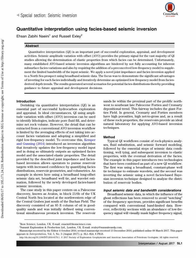
Quantitative interpretation using facies-based seismic inversion

Ehsan Zabihi Naeini1 and Russell Exley2

Abstract

Quantitative interpretation (QI) is an important part of successful exploration, appraisal, and developmentactivities. Seismic amplitude variation with offset (AVO) provides the primary signal for the vast majority of QIstudies allowing the determination of elastic properties from which facies can be determined. Unfortunately,many established AVO-based seismic inversion algorithms are hindered by not fully accounting for inherentsubsurface facies variations and also by requiring the addition of a preconceived low-frequency model to supple-ment the limited bandwidth of the input seismic. We apply a novel joint impedance and facies inversion appliedto a North Sea prospect using broadband seismic data. The focus was to demonstrate the significant advantagesof inverting for each facies individually and iteratively determine an optimized low-frequency model from facies-derived depth trends. The results generated several scenarios for potential facies distributions thereby providingguidance to future appraisal and development decisions.

IntroductionDerisking via quantitative interpretation (QI) is an

essential part of successful hydrocarbon explorationand appraisal. In ideal circumstances, QI using ampli-tude variation with offset (AVO) inversion can be usedto identify lithologies, indicate pore fluid fill, and deter-mine net rock volume. However, the detail that can beextracted from a conventional AVO inversion workflowis limited by the averaging effects of not taking into ac-count facies variations and adopting a simplified andrigid low-frequency model. To overcome this, Kemperand Gunning (2014) introduced an inversion algorithmthat iteratively updates the low-frequency model inputand in doing so ultimately outputs an optimized faciesmodel and the associated elastic properties. The detailprovided by the described joint impedance and facies-based inversion allows operators to pursue reservoirtargets with increased confidence by quantifying faciesdistributions, reservoir geometries, and volumetrics. Anexample is shown here using a broadband long-offsetseismic data set, broadband well tie, and wavelet esti-mation, followed by the newly developed facies-basedseismic inversion.

The case study in this paper centers on a Paleocenediscovery, known as Avalon, in block 21/6b of the UKCentral North Sea located at the northwestern edge ofthe Central Graben just south of the Buchan Field. Thediscovery consisted of an 85 ft column of oil in good-quality sands and was initially defined using conven-tional simultaneous prestack inversion. The reservoir

sands lie within the proximal part of the prolific north-west to southeast late Paleocene Forties and Cromartydepositional trend. This fairway includes the giant For-ties Field. In general, Cromarty and Forties membershave high porosities, high net-to-gross and, as a resultof these rock properties, the reservoirs provide an idealnatural laboratory for applying AVO-based inversiontechniques.

MethodTypical QI workflows consist of rock-physics analy-

ses, fluid substitution, and seismic forward modeling,followed by the essential steps of seismic data condi-tioning, well tying, and subsequent inversion to elasticproperties, with the eventual derivation of the facies.The example in this paper introduces two technologiesthat have been combined as part of a new QI workflow.The first was using a broadband, constant-phase welltie technique to estimate wavelets, and the second wasinverting the seismic using a novel facies-based Baye-sian inversion technique designed to analyze the distri-bution of reservoir bodies.

Input seismic data and bandwidth considerationsBroadband seismic data, in which the influence of the

ghost reflections has been removed to avoid “notching”of the frequency spectrum, provides significant benefitscompared with conventional band-limited data. How-ever, reflectivity sections with an abundance of low-fre-quency signal will visually mask higher frequency signal,

1Ikon Science, London, UK. E-mail: enaeini@ikonscience.com.2Summit Exploration & Production Ltd., London, UK. E-mail: rexley@summiteandp.com.Manuscript received by the Editor 4 October 2016; revised manuscript received 13 December 2016; published online 09 March 2017. This paper

appears in Interpretation, Vol. 5, No. 3 (August 2017); p. SL1–SL8, 8 FIGS.http://dx.doi.org/10.1190/INT-2016-0178.1. © 2017 Society of Exploration Geophysicists and American Association of Petroleum Geologists. All rights reserved.

t

Special section: Seismic inversion

Interpretation / August 2017 SL1Interpretation / August 2017 SL1

Dow

nloa

ded

06/0

5/17

to 1

95.1

71.2

4.21

0. R

edis

trib

utio

n su

bjec

t to

SEG

lice

nse

or c

opyr

ight

; see

Ter

ms

of U

se a

t http

://lib

rary

.seg

.org

/

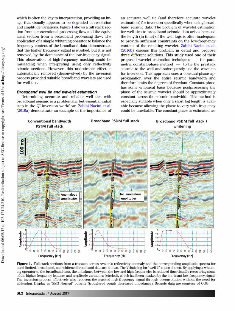
which is often the key to interpretation, providing an im-age that visually appears to be degraded in resolutionand amplitude variations. Figure 1 shows a full stack sec-tion from a conventional processing flow and the equiv-alent section from a broadband processing flow. Theapplication of a simple whitening operator to balance thefrequency content of the broadband data demonstratesthat the higher frequency signal is masked, but it is notremoved, by the dominance of the low-frequency signal.This observation of high-frequency masking could bemisleading when interpreting using only reflectivityseismic sections. However, this undesirable effect isautomatically removed (deconvolved) by the inversionprocess provided suitable broadband wavelets are usedfor well ties.

Broadband well tie and wavelet estimationDetermining accurate and reliable well ties with

broadband seismic is a problematic but essential initialstep in the QI inversion workflow. Zabihi Naeini et al.(2016a) demonstrate an example of the importance of

an accurate well tie (and therefore accurate waveletestimation) for inversion specifically when using broad-band seismic data. The problem of wavelet estimationfor well ties to broadband seismic data arises becausethe length (in time) of the well logs is often inadequateto provide sufficient constraints on the low-frequencycontent of the resulting wavelet. Zabihi Naeini et al.(2016b) discuss this problem in detail and proposethree different solutions. This study used one of theirproposed wavelet estimation techniques — the para-metric constant-phase method — to tie the prestackseismic to the well and subsequently use the waveletsfor inversion. This approach uses a constant-phase ap-proximation over the entire seismic bandwidth andtherefore limits the degrees of freedom. Constant phasehas some empirical basis because postprocessing thephase of the seismic wavelet should be approximatelyconstant across the seismic bandwidth. This method isespecially suitable when only a short log length is avail-able because allowing the phase to vary with frequencycould be unreliable. The constant phase is estimated us-

Figure 1. Full-stack sections from a transect across Avalon’s reflectivity anomaly and the corresponding amplitude spectra forband-limited, broadband, and whitened broadband data are shown. The Vshale log for “well 2” is also shown. By applying a whiten-ing operator to the broadband data, the imbalance between the low and high frequencies is reduced thus visually recovering someof the higher frequency features and amplitude variations (circled), which had been masked by the dominant low-frequency signal.The inversion process effectively also recovers the masked high-frequency signal through deconvolution without the need forwhitening. Display in “SEG Normal” polarity (trough/red equals decreased impedance). Seismic data are courtesy of CGG.

SL2 Interpretation / August 2017

Dow

nloa

ded

06/0

5/17

to 1

95.1

71.2

4.21

0. R

edis

trib

utio

n su

bjec

t to

SEG

lice

nse

or c

opyr

ight

; see

Ter

ms

of U

se a

t http

://lib

rary

.seg

.org

/

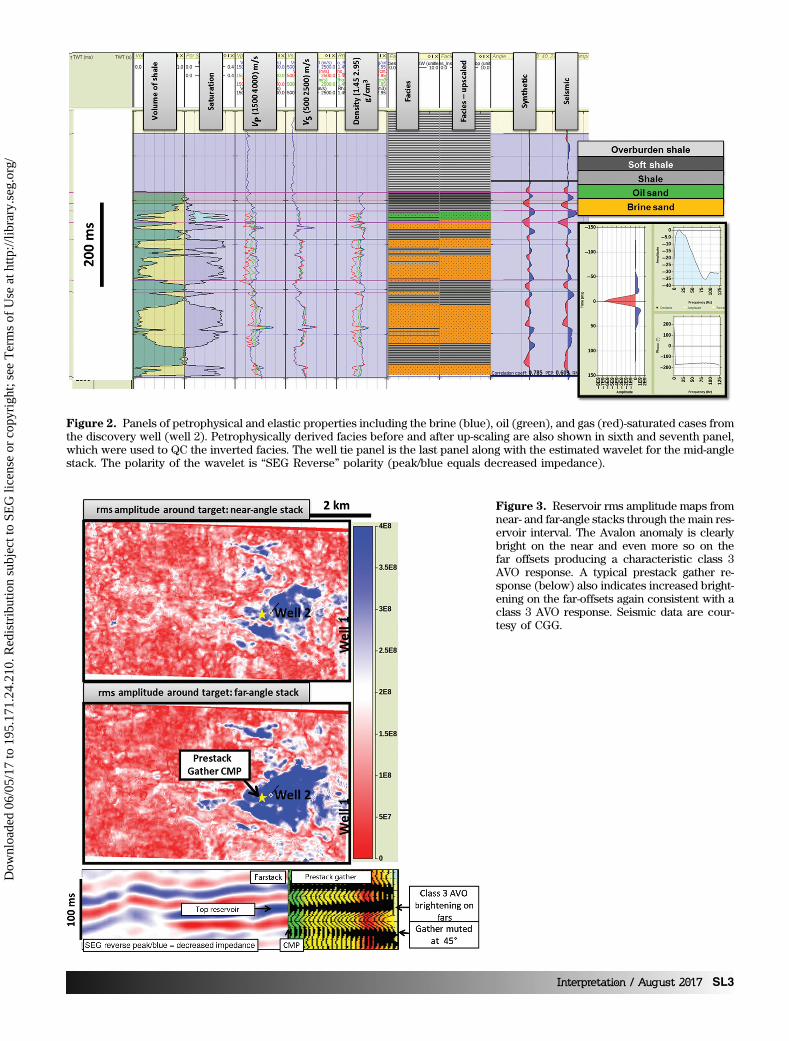
Figure 2. Panels of petrophysical and elastic properties including the brine (blue), oil (green), and gas (red)-saturated cases fromthe discovery well (well 2). Petrophysically derived facies before and after up-scaling are also shown in sixth and seventh panel,which were used to QC the inverted facies. The well tie panel is the last panel along with the estimated wavelet for the mid-anglestack. The polarity of the wavelet is “SEG Reverse” polarity (peak/blue equals decreased impedance).

Figure 3. Reservoir rms amplitude maps fromnear- and far-angle stacks through the main res-ervoir interval. The Avalon anomaly is clearlybright on the near and even more so on thefar offsets producing a characteristic class 3AVO response. A typical prestack gather re-sponse (below) also indicates increased bright-ening on the far-offsets again consistent with aclass 3 AVO response. Seismic data are cour-tesy of CGG.

Interpretation / August 2017 SL3

Dow

nloa

ded

06/0

5/17

to 1

95.1

71.2

4.21

0. R

edis

trib

utio

n su

bjec

t to

SEG

lice

nse

or c

opyr

ight

; see

Ter

ms

of U

se a

t http

://lib

rary

.seg

.org

/

ing a least-squares-based method over a long but taperedinterval of seismic data to derive a stable amplitude spec-trum using multiple traces around available wells.

Facies-based seismic inversionFacies-based seismic inversion, in which the low-

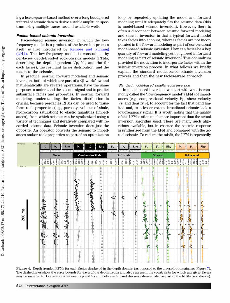
frequency model is a product of the inversion processitself, is first introduced by Kemper and Gunning(2014). The low-frequency model is constrained byper-facies depth-trended rock-physics models (RPMs;describing the depth-dependent Vp, Vs, and rho foreach facies), the resultant facies distribution, and thematch to the seismic.

In practice, seismic forward modeling and seismicinversion, both of which are part of a QI workflow andmathematically are reverse operations, have the samepurpose: to understand the seismic signal and to predictsubsurface facies and properties. In seismic forwardmodeling, understanding the facies distribution iscrucial, because per-facies RPMs can be used to trans-form rock properties (e.g., porosity, volume of shale,hydrocarbon saturation) to elastic quantities (imped-ances), from which seismic can be synthesized using avariety of techniques and iteratively compared with re-corded seismic data. Seismic inversion does just theopposite: An operator converts the seismic to imped-ances and/or rock properties as part of an optimization

loop by repeatedly updating the model and forwardmodeling until it adequately fits the seismic data (thisis model-based seismic inversion). However, there isoften a disconnect between seismic forward modelingand seismic inversion in that a typical forward modeltakes facies into account, whereas facies are not incor-porated in the forward modeling as part of conventionalmodel-based seismic inversion. How can facies be a keyquantity of forward modeling yet be ignored in forwardmodeling as part of seismic inversion? This conundrumprovided the motivation to incorporate facies within theseismic inversion process. In what follows we brieflyexplain the standard model-based seismic inversionprocess and then the new facies-aware approach.

Standard model-based simultaneous inversionIn model-based inversion, we start with what is com-

monly called the “low-frequency model” (LFM) of imped-ances (e.g., compressional velocity Vp, shear velocityVs, and density ρ), to account for the fact that band lim-ited and, to a lesser extent, broadband seismic lack alow-frequency signal. It is worth noting that the qualityof this LFM is oftenmuchmore important than the actualinversion algorithm used. There are many such algo-rithms available, but in essence the seismic responseis synthesized from the LFM and compared with the ac-tual seismic. To reduce the misfit, the LFM is repeatedly

Figure 4. Depth-trended RPMs for each facies displayed in the depth domain (as opposed to the crossplot domain; see Figure 7).The dashed lines show the error bounds for each of the depth trends and also represent the constraints for which any given faciesmay be inverted to. Correlations between Vp and Vs and between Vp and rho were derived also as part of the RPMs (not shown).

SL4 Interpretation / August 2017

Dow

nloa

ded

06/0

5/17

to 1

95.1

71.2

4.21

0. R

edis

trib

utio

n su

bjec

t to

SEG

lice

nse

or c

opyr

ight

; see

Ter

ms

of U

se a

t http

://lib

rary

.seg

.org

/

updated, seismic resynthesized (using forward model-ing), and recompared. Once the misfit is minimized, theprocess stops and the last model of impedances is theinversion result. Facies are not considered at any pointin this process.

The problem with the above process is in the con-struction of the initial LFM, the most important inputto this process. The starting model should have a gentlyvarying vertical profile of sand impedance values inwhich sand is present (typically hardening because ofcompaction), and the same for other facies. But priorto the inversion, the location of the various facies isof course unknown; hence, it is not possible to assignthe correct initial impedance value to the LFM at anygiven point. In practice, we end up with a compromiseof impedance values (e.g., average impedance of differ-ent facies) unrepresentative of any particular facies,which degrades the inversion result.

The problem of facies variations is particularly evi-dent when building the LFM by interpolation of wellimpedance profiles along interpreted seismic horizons(the typical form of LFM construction). At one well, wemay have sand of a particular seismo-stratigraphic age,and in another well, we may have shale of the same age.Interpolation between these two wells produces com-promised, neither-sand-nor-shale impedance values inthe LFM and the subsequent seismic inversion cannotcorrect this error of low-frequency input bias as theseismic lacks low-frequency signal.

A new approach: Facies-aware model-based inversionTo improve the construction of the LFM, we input mul-

tiple, simple LFMs, one for each expected facies (i.e., weoverspecify the low-frequency information). In its simplestform,we plot impedance log data as a function of depth be-low an appropriate datum restricted to a particular facies,and then we fit a compaction curve to that data, completewith an assessment of uncertainty. In three dimensions,wecan take thehorizon representing thedatum,and “hang”the compaction curve off that horizon at all trace locations.

In this new approach, the inversion derives models ofinitial impedances (from the seismic) and then determinesthe facies during each iteration of the optimization loop.The facies result depends on the last set of impedance re-sults, but here we focus on how the impedance results(inverted from the seismic data) depend on the last faciesresult (of the previous iteration). For this step, an LFM ofimpedances is required; this is reconstructed at each iter-ation from the various per-facies LFMs as follows:

1) Start with an empty LFM.2) Where the last, most up-to-date facies model indi-

cates there is sand, copy the sand into the LFM, par-tially populating the LFM.

3) Repeat for the other facies until the LFM is entirelypopulated.

The final LFM is therefore not a static input as instandard model-based simultaneous inversion, but it

is the seismically driven output of the new inversionsystem, which incorporates known facies. Therefore,the main outputs of the inversion are the elastic proper-ties and facies. Kemper and Gunning (2014) describethe mechanics of this new algorithm more fully.

North Sea case studyIn this study, the input seismic was conventionally

acquired but broadband processed, which consistedof two important processing steps. First, a preimaging3D source- and receiver-side deghosting technique(Wang et al., 2013), for broadening the bandwidth ofthe conventionally acquired towed streamer data, wasused to remove the frequency notches caused by ghost

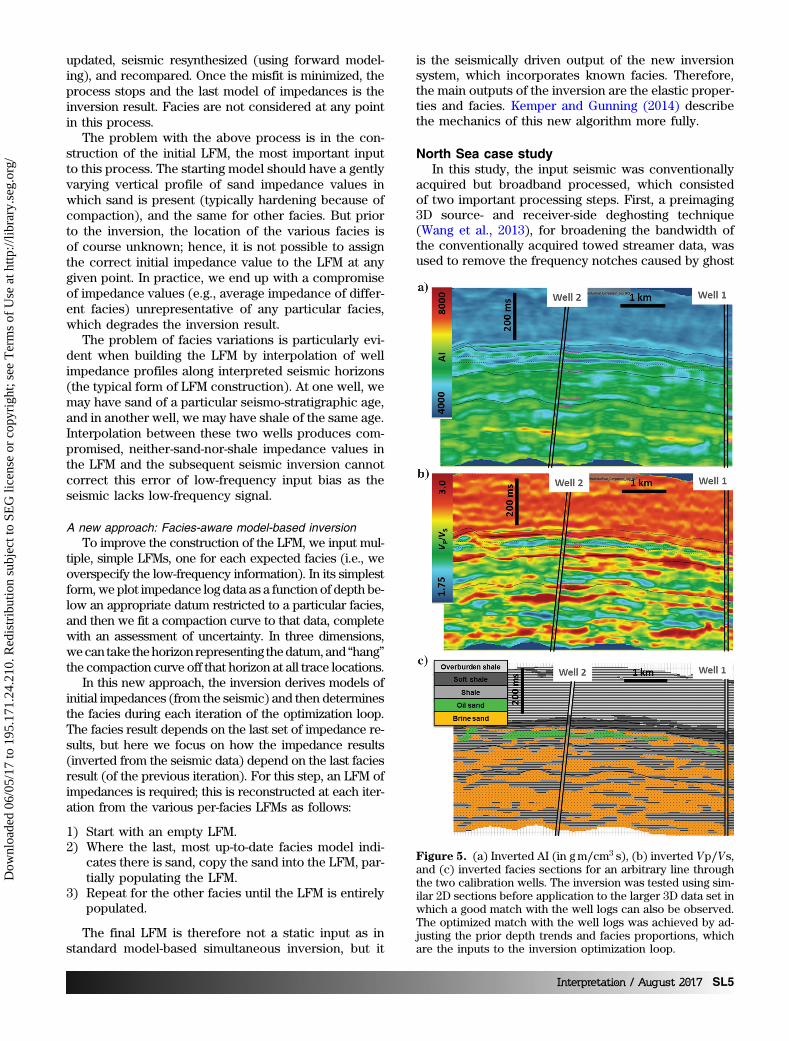
Figure 5. (a) Inverted AI (in gm∕cm3 s), (b) inverted Vp∕Vs,and (c) inverted facies sections for an arbitrary line throughthe two calibration wells. The inversion was tested using sim-ilar 2D sections before application to the larger 3D data set inwhich a good match with the well logs can also be observed.The optimized match with the well logs was achieved by ad-justing the prior depth trends and facies proportions, whichare the inputs to the inversion optimization loop.

Interpretation / August 2017 SL5

Dow

nloa

ded

06/0

5/17

to 1

95.1

71.2

4.21

0. R

edis

trib

utio

n su

bjec

t to

SEG

lice

nse

or c

opyr

ight

; see

Ter

ms

of U

se a

t http

://lib

rary

.seg

.org

/

wavelet interference. Second, the processing workflowincluded a multilayer, nonlinear, slope tomography(Guillaume et al., 2013) to derive the velocity modelfor imaging and Kirchhoff prestack depth migration(PSDM) before stretching the data back to the time do-main. Using such broadband seismic data increases thelow- and high-frequency signal, thereby enhancing theresolution (Zabihi Naeini et al., 2015). Improved lowfrequencies within the seismic are especially importantfor seismic inversion because they reduce the depend-ency on the initial low-frequency information.

Figure 2 shows the well tie panel and the estimatedwavelet, using the aforementioned constant-phasemethod, for the mid-angle stack. One can observe rea-sonable low-frequency decay on the amplitude spectrumobtained as part of the broadband wavelet estimationtechnique by using multitaper spectral smoothing andaveraging over many traces around the well. The welltie workflow included a blind QC in which the waveletwas estimated at one well and used to tie the secondwell. After completing this process, a good-quality welltie can be observed with a crosscorrelation coefficient of0.78 and a phase error of approximately 10°. Similar qual-ity well ties were also achieved for the other angle stacksand at the other well in this study.

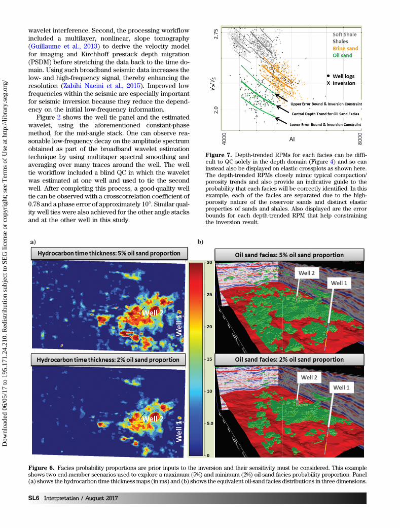
Figure 7. Depth-trended RPMs for each facies can be diffi-cult to QC solely in the depth domain (Figure 4) and so caninstead also be displayed on elastic crossplots as shown here.The depth-trended RPMs closely mimic typical compaction/porosity trends and also provide an indicative guide to theprobability that each facies will be correctly identified. In thisexample, each of the facies are separated due to the high-porosity nature of the reservoir sands and distinct elasticproperties of sands and shales. Also displayed are the errorbounds for each depth-trended RPM that help constrainingthe inversion result.

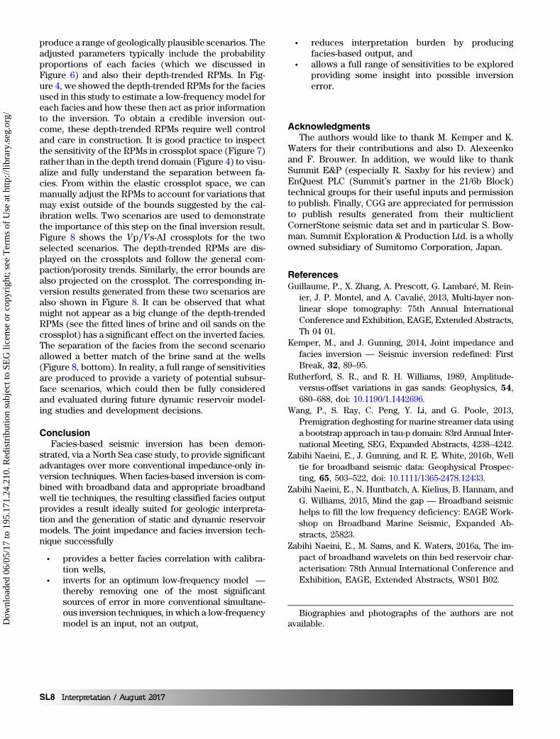
Figure 6. Facies probability proportions are prior inputs to the inversion and their sensitivity must be considered. This exampleshows two end-member scenarios used to explore a maximum (5%) and minimum (2%) oil-sand facies probability proportion. Panel(a) shows the hydrocarbon time thicknessmaps (in ms) and (b) shows the equivalent oil-sand facies distributions in three dimensions.

SL6 Interpretation / August 2017

Dow

nloa

ded

06/0

5/17

to 1

95.1

71.2

4.21

0. R

edis

trib

utio

n su

bjec

t to

SEG

lice

nse

or c

opyr

ight

; see

Ter

ms

of U

se a

t http

://lib

rary

.seg

.org

/

Initial rock-physics and forward-modeling studies re-vealed that the Avalon discovery exhibited a “textbook”class 3 AVO (Rutherford and Williams, 1989) anomalyfrom the top reservoir reflector. Figure 3 shows a typ-ical prestack gather and resulting poststack rms ampli-tude maps from around the Avalon discovery for thenear and far partial angle stacks. The main reservoiranomaly is evident around well 2.

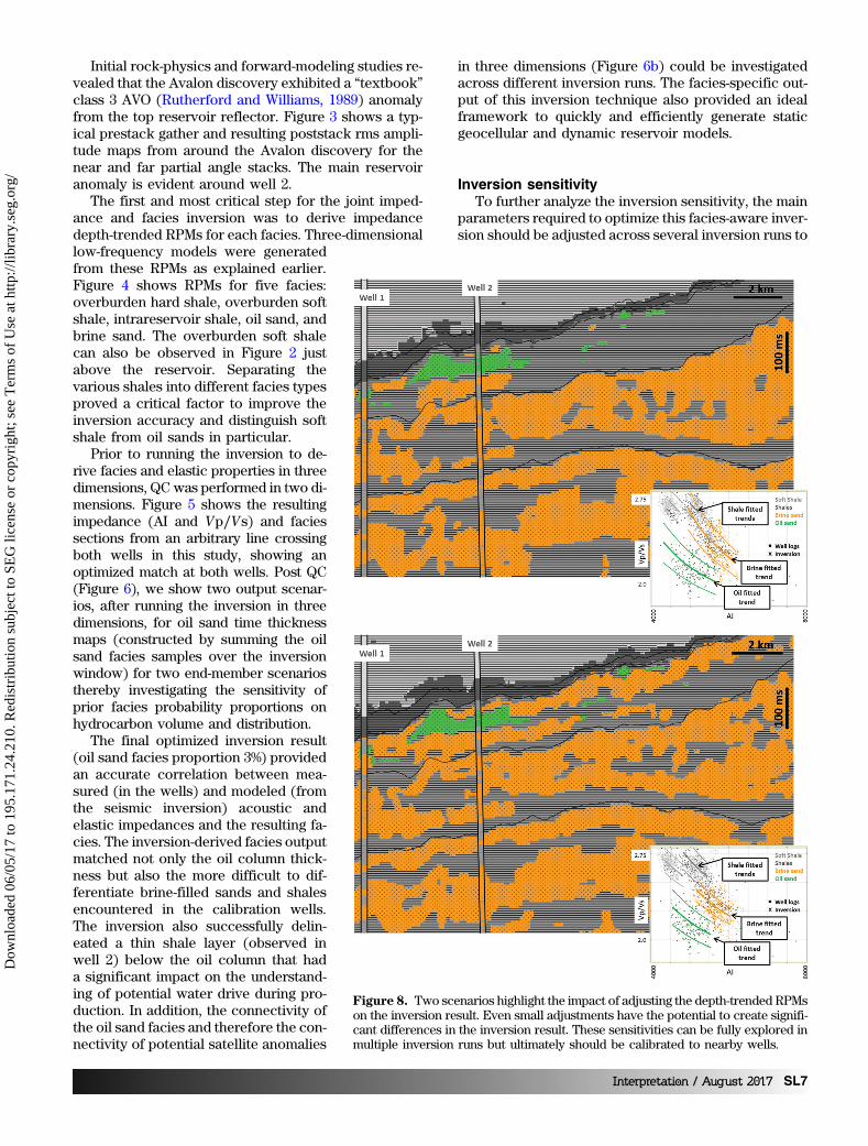
The first and most critical step for the joint imped-ance and facies inversion was to derive impedancedepth-trended RPMs for each facies. Three-dimensionallow-frequency models were generatedfrom these RPMs as explained earlier.Figure 4 shows RPMs for five facies:overburden hard shale, overburden softshale, intrareservoir shale, oil sand, andbrine sand. The overburden soft shalecan also be observed in Figure 2 justabove the reservoir. Separating thevarious shales into different facies typesproved a critical factor to improve theinversion accuracy and distinguish softshale from oil sands in particular.

Prior to running the inversion to de-rive facies and elastic properties in threedimensions, QCwas performed in two di-mensions. Figure 5 shows the resultingimpedance (AI and Vp∕Vs) and faciessections from an arbitrary line crossingboth wells in this study, showing anoptimized match at both wells. Post QC(Figure 6), we show two output scenar-ios, after running the inversion in threedimensions, for oil sand time thicknessmaps (constructed by summing the oilsand facies samples over the inversionwindow) for two end-member scenariosthereby investigating the sensitivity ofprior facies probability proportions onhydrocarbon volume and distribution.

The final optimized inversion result(oil sand facies proportion 3%) providedan accurate correlation between mea-sured (in the wells) and modeled (fromthe seismic inversion) acoustic andelastic impedances and the resulting fa-cies. The inversion-derived facies outputmatched not only the oil column thick-ness but also the more difficult to dif-ferentiate brine-filled sands and shalesencountered in the calibration wells.The inversion also successfully delin-eated a thin shale layer (observed inwell 2) below the oil column that hada significant impact on the understand-ing of potential water drive during pro-duction. In addition, the connectivity ofthe oil sand facies and therefore the con-nectivity of potential satellite anomalies

in three dimensions (Figure 6b) could be investigatedacross different inversion runs. The facies-specific out-put of this inversion technique also provided an idealframework to quickly and efficiently generate staticgeocellular and dynamic reservoir models.

Inversion sensitivityTo further analyze the inversion sensitivity, the main

parameters required to optimize this facies-aware inver-sion should be adjusted across several inversion runs to

Figure 8. Two scenarios highlight the impact of adjusting the depth-trended RPMson the inversion result. Even small adjustments have the potential to create signifi-cant differences in the inversion result. These sensitivities can be fully explored inmultiple inversion runs but ultimately should be calibrated to nearby wells.

Interpretation / August 2017 SL7

Dow

nloa

ded

06/0

5/17

to 1

95.1

71.2

4.21

0. R

edis

trib

utio

n su

bjec

t to

SEG

lice

nse

or c

opyr

ight

; see

Ter

ms

of U

se a

t http

://lib

rary

.seg

.org

/

produce a range of geologically plausible scenarios. Theadjusted parameters typically include the probabilityproportions of each facies (which we discussed inFigure 6) and also their depth-trended RPMs. In Fig-ure 4, we showed the depth-trended RPMs for the faciesused in this study to estimate a low-frequency model foreach facies and how these then act as prior informationto the inversion. To obtain a credible inversion out-come, these depth-trended RPMs require well controland care in construction. It is good practice to inspectthe sensitivity of the RPMs in crossplot space (Figure 7)rather than in the depth trend domain (Figure 4) to visu-alize and fully understand the separation between fa-cies. From within the elastic crossplot space, we canmanually adjust the RPMs to account for variations thatmay exist outside of the bounds suggested by the cal-ibration wells. Two scenarios are used to demonstratethe importance of this step on the final inversion result.Figure 8 shows the Vp∕Vs-AI crossplots for the twoselected scenarios. The depth-trended RPMs are dis-played on the crossplots and follow the general com-paction/porosity trends. Similarly, the error bounds arealso projected on the crossplot. The corresponding in-version results generated from these two scenarios arealso shown in Figure 8. It can be observed that whatmight not appear as a big change of the depth-trendedRPMs (see the fitted lines of brine and oil sands on thecrossplot) has a significant effect on the inverted facies.The separation of the facies from the second scenarioallowed a better match of the brine sand at the wells(Figure 8, bottom). In reality, a full range of sensitivitiesare produced to provide a variety of potential subsur-face scenarios, which could then be fully consideredand evaluated during future dynamic reservoir model-ing studies and development decisions.

ConclusionFacies-based seismic inversion has been demon-

strated, via a North Sea case study, to provide significantadvantages over more conventional impedance-only in-version techniques. When facies-based inversion is com-bined with broadband data and appropriate broadbandwell tie techniques, the resulting classified facies outputprovides a result ideally suited for geologic interpreta-tion and the generation of static and dynamic reservoirmodels. The joint impedance and facies inversion tech-nique successfully

• provides a better facies correlation with calibra-tion wells,

• inverts for an optimum low-frequency model —

thereby removing one of the most significantsources of error in more conventional simultane-ous inversion techniques, in which a low-frequencymodel is an input, not an output,

• reduces interpretation burden by producingfacies-based output, and

• allows a full range of sensitivities to be exploredproviding some insight into possible inversionerror.

AcknowledgmentsThe authors would like to thank M. Kemper and K.

Waters for their contributions and also D. Alexeenkoand F. Brouwer. In addition, we would like to thankSummit E&P (especially R. Saxby for his review) andEnQuest PLC (Summit’s partner in the 21/6b Block)technical groups for their useful inputs and permissionto publish. Finally, CGG are appreciated for permissionto publish results generated from their multiclientCornerStone seismic data set and in particular S. Bow-man. Summit Exploration & Production Ltd. is a whollyowned subsidiary of Sumitomo Corporation, Japan.

ReferencesGuillaume, P., X. Zhang, A. Prescott, G. Lambaré, M. Rein-

ier, J. P. Montel, and A. Cavalié, 2013, Multi-layer non-linear slope tomography: 75th Annual InternationalConference and Exhibition, EAGE, Extended Abstracts,Th 04 01.

Kemper, M., and J. Gunning, 2014, Joint impedance andfacies inversion — Seismic inversion redefined: FirstBreak, 32, 89–95.

Rutherford, S. R., and R. H. Williams, 1989, Amplitude-versus-offset variations in gas sands: Geophysics, 54,680–688, doi: 10.1190/1.1442696.

Wang, P., S. Ray, C. Peng, Y. Li, and G. Poole, 2013,Premigration deghosting for marine streamer data usinga bootstrap approach in tau-p domain: 83rd Annual Inter-national Meeting, SEG, Expanded Abstracts, 4238–4242.

Zabihi Naeini, E., J. Gunning, and R. E. White, 2016b, Welltie for broadband seismic data: Geophysical Prospec-ting, 65, 503–522, doi: 10.1111/1365-2478.12433.

Zabihi Naeini, E., N. Huntbatch, A. Kielius, B. Hannam, andG. Williams, 2015, Mind the gap — Broadband seismichelps to fill the low frequency deficiency: EAGE Work-shop on Broadband Marine Seismic, Expanded Ab-stracts, 25823.

Zabihi Naeini, E., M. Sams, and K. Waters, 2016a, The im-pact of broadband wavelets on thin bed reservoir char-acterisation: 78th Annual International Conference andExhibition, EAGE, Extended Abstracts, WS01 B02.

Biographies and photographs of the authors are notavailable.

SL8 Interpretation / August 2017

Dow

nloa

ded

06/0

5/17

to 1

95.1

71.2

4.21

0. R

edis

trib

utio

n su

bjec

t to

SEG

lice

nse

or c

opyr

ight

; see

Ter

ms

of U

se a

t http

://lib

rary

.seg

.org

/