Quantum Field Theory II

Lecture Notes

ETH Zurich, FS13

Prof. N. Beisert

c© 2013 Niklas Beisert, ETH Zurich

This document as well as its parts is protected by copyright.Reproduction of any part in any form without prior writtenconsent of the author is permissible only for private,scientific and non-commercial use.

Contents

0 Overview 40.1 Prerequisites . . . . . . . . . . . . . . . . . . . . . . . . . . . . . . . 50.2 Contents . . . . . . . . . . . . . . . . . . . . . . . . . . . . . . . . . 50.3 References . . . . . . . . . . . . . . . . . . . . . . . . . . . . . . . . 5

1 Path Integral for Quantum Mechanics 1.11.1 Motivation . . . . . . . . . . . . . . . . . . . . . . . . . . . . . . . . 1.11.2 Path Integral for Transition Amplitude . . . . . . . . . . . . . . . . 1.51.3 Free Particle . . . . . . . . . . . . . . . . . . . . . . . . . . . . . . . 1.101.4 Operator Insertions . . . . . . . . . . . . . . . . . . . . . . . . . . . 1.11

2 Path Integral for Fields 2.12.1 Time-Ordered Correlators . . . . . . . . . . . . . . . . . . . . . . . 2.12.2 Sources and Generating Functional . . . . . . . . . . . . . . . . . . 2.22.3 Fermionic Integrals . . . . . . . . . . . . . . . . . . . . . . . . . . . 2.62.4 Interactions . . . . . . . . . . . . . . . . . . . . . . . . . . . . . . . 2.92.5 Further Generating Functionals . . . . . . . . . . . . . . . . . . . . 2.14

3 Lie Algebra 3.13.1 Lie Groups . . . . . . . . . . . . . . . . . . . . . . . . . . . . . . . . 3.13.2 Lie Algebras . . . . . . . . . . . . . . . . . . . . . . . . . . . . . . . 3.23.3 Enveloping Algebras . . . . . . . . . . . . . . . . . . . . . . . . . . 3.53.4 Representations . . . . . . . . . . . . . . . . . . . . . . . . . . . . . 3.63.5 Invariants . . . . . . . . . . . . . . . . . . . . . . . . . . . . . . . . 3.103.6 Unitary and Other Algebras . . . . . . . . . . . . . . . . . . . . . . 3.13

4 Yang–Mills Theory 4.14.1 Classical Gauge Theory . . . . . . . . . . . . . . . . . . . . . . . . . 4.14.2 Abelian Quantisation Revisited . . . . . . . . . . . . . . . . . . . . 4.64.3 Yang–Mills Quantisation . . . . . . . . . . . . . . . . . . . . . . . . 4.94.4 Feynman Rules . . . . . . . . . . . . . . . . . . . . . . . . . . . . . 4.134.5 BRST Symmetry . . . . . . . . . . . . . . . . . . . . . . . . . . . . 4.16

5 Renormalisation 5.15.1 Dimensional Regularisation . . . . . . . . . . . . . . . . . . . . . . 5.15.2 Renormalisation . . . . . . . . . . . . . . . . . . . . . . . . . . . . . 5.55.3 Renormalisation Flow . . . . . . . . . . . . . . . . . . . . . . . . . . 5.13

6 Quantum Symmetries 6.16.1 Schwinger–Dyson Equations . . . . . . . . . . . . . . . . . . . . . . 6.16.2 Slavnov–Taylor Identities . . . . . . . . . . . . . . . . . . . . . . . . 6.36.3 Ward–Takahashi Identity . . . . . . . . . . . . . . . . . . . . . . . . 6.56.4 Anomalies . . . . . . . . . . . . . . . . . . . . . . . . . . . . . . . . 6.8

7 Spontaneous Symmetry Breaking 7.17.1 Breaking of Global Symmetries . . . . . . . . . . . . . . . . . . . . 7.1

3

7.2 Breaking of Gauge Symmetries . . . . . . . . . . . . . . . . . . . . 7.57.3 Electroweak Model . . . . . . . . . . . . . . . . . . . . . . . . . . . 7.9

4

Quantum Field Theory II Chapter 0ETH Zurich, FS13 Prof. N. Beisert

26. 05. 2013

0 Overview

After having learned the basic concepts of Quantum Field Theory in QFT I, wecan now go on to complete the foundations of QFT in QFT II. The aim of thislecture course is to be able to formulate the Standard Model of Particle Physicsand perform calculations in it. We shall cover the following topics:

• path integral• non-abelian gauge theory• renormalisation• symmetries• spontaneous symmetry breaking

More concretely, the topics can be explained as follows:

Path Integral. In QFT I we have applied the canonical quantisation frameworkto fields. The path integral is an alternative framework for performing equivalentcomputations. In many situations it is more direct, more efficient or simply moreconvenient to use. It is however not built upon the common intuition of quantummechanics.

Non-Abelian Gauge Theory. We have already seen how to formulate thevector field for use in electrodynamics. The vector field for chromodynamics issimilar, but it adds the important concept of self-interactions which makes thefield have a very different physics. The underlying model is called non-abeliangauge theory or Yang–Mills theory.

Renormalisation. We will take a fresh look at renormalisation, in particularconcerning the consistency of gauge theory and the global features ofrenormalisation transformations.

Symmetries. We will consider how symmetries work in the path integralframework. This will also give us some awareness of quantum violations ofsymmetry, so-called anomalies.

Spontaneous Symmetry Breaking. The electroweak interactions aremediated by massive vector particles. Naive they lead to non-renormalisablemodels, but by considering spontaneous symmetry breaking one can accommodatethem in gauge theories.

5

0.1 Prerequisites

• Quantum Field Theory I (concepts, start from scratch)• classical and quantum mechanics• electrodynamics, mathematical methods in physics

0.2 Contents

1. Path Integral for Quantum Mechanics (3 lectures)2. Path Integral for Fields (7 lectures)3. Lie Algebra (5 lectures)4. Yang–Mills Theory (6 lectures)5. Renormalisation (6 lectures)6. Quantum Symmetries (4 lectures)7. Spontaneous Symmetry Breaking (5 lectures)

Indicated are the approximate number of 45-minute lectures. Altogether, thecourse consists of 37 lectures which includes one overview lecture.

0.3 References

There are many text books and lecture notes on quantum field theory. Here is aselection of well-known ones:

• M. E. Peskin, D. V. Schroeder, “An Introduction to Quantum Field Theory”,Westview Press (1995)• C. Itzykson, J.-B. Zuber, “Quantum Field Theory”, McGraw-Hill (1980)• P. Ramond, “Field Theory: A Modern Primer”, Westview Press (1990)• M. Srendnicki, “Quantum Field Theory”, Cambridge University Press (2007)• M. Kaku, “Quantum Field Theory”, Oxford University Press (1993)• online: M. Gaberdiel, A. Gehrmann-De Ridder, “Quantum Field Theory II”,

lecture notes,http://www.itp.phys.ethz.ch/research/qftstrings/archive/11FSQFT2

6

Quantum Field Theory II Chapter 1ETH Zurich, FS13 Prof. N. Beisert

17. 12. 2013

1 Path Integral for Quantum Mechanics

We start the lecture course by introducing the path integral in the simple settingof quantum mechanics in canonical quantisation.

1.1 Motivation

The path integral is framework to formulate quantum theories. It was developedmainly by Dirac (1933) and Feynman (1948). It is particularly useful forrelativistic quantum field theory.

Why? In QFT I we have relied on canonical quantisation to formulate aquantum theory of relativistic fields. During the first half of that course, we haveencountered and overcome several difficulties in quantising scalar, spinor andvector fields.

• Canonical quantisation is intrinsically not relativistically covariant due to thespecialisation of time. Nevertheless, at the end of the day, results turned outcovariant as they should. In between, we had to manipulate some intransparentexpressions.• Gauge fixing the massless vector field was not exactly fun.• Canonical quantisation is based on non-commuting field operators. The operator

algebra makes manipulations rather tedious.• Moreover one has to deal with ordering ambiguities when quantising a classical

expression.• Despite their final simplicity, deriving Feynman rules was a long effort.• We can treat interacting models perturbatively, but it is hard to formulate what

finite or strong coupling means.

The path integral method avoids many of the above problems:

• It does not single out a particular time or relativistic frame in any way. A priori,it is a fully covariant framework.• It uses methods of functional analysis rather than operator algebra. The

fundamental quantities are perfectly commuting objects (or sometimeanti-commuting Grassmann numbers).• It is based directly on the classical action functional. Operator ordering issues do

not have to be considered (although there is an equivalent of operator ordering).• Gauge fixing for massless vector fields has a few complications which are

conveniently treated in the path integral framework.• Feynman rules can be derived directly and conveniently.• The path integral can be formulated well for finite or strong coupling, and some

information can sometimes be extracted (yet the methods of calculation areusually to the perturbative regime).

1.1

• It is a different formulation and interpretation of quantum theories.

Why Not? In fact, one could directly use the path integral to formulate aquantum theory without first performing canonical quantisation. There arehowever a few shortcoming of the path integral which are good reasons tounderstand the canonical framework:

• The notion of states is not as evident in the path integral.• Similarly, operators and their algebras are not natural concepts of the path

integral.• Therefore, the central feature of unitarity remains obscure in the path integral.• Canonical quantisation of fields connects immediately to the conventional

treatment of quantum mechanics.

Multiple Slits. But what is the path integral? It is a method to compute theinterference of quantum mechanical waves by considering all trajectories.

A standard way to illustrate the path integral is to consider multiple-slitinterference patterns: Consider a source which emits particles or waves to a screenwhere they will be detected. Suppose the particles have a well-defined de Brogliewavelength λ. We then insert hard obstacles into the path and observe theinterference pattern on the screen.

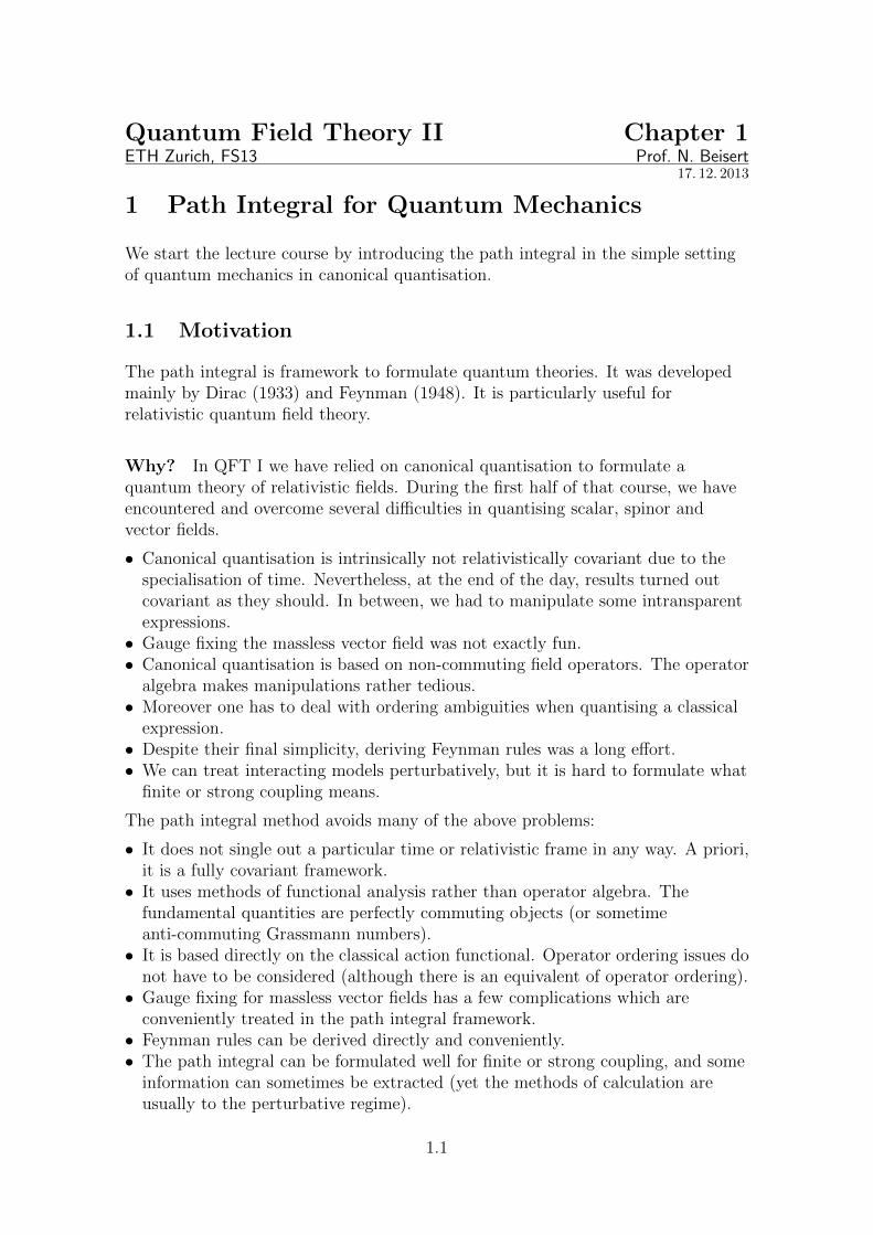
Suppose we first put an obstacle with a single slit.

(1.1)

A sufficiently small slit (compared to λ) would act as a new point-like source, andwe would observe no structures on the screen.1

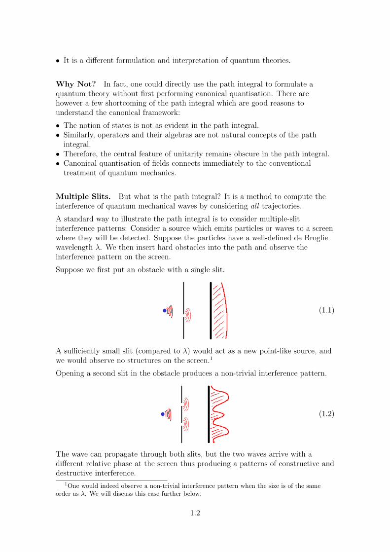
Opening a second slit in the obstacle produces a non-trivial interference pattern.

(1.2)

The wave can propagate through both slits, but the two waves arrive with adifferent relative phase at the screen thus producing a patterns of constructive anddestructive interference.

1One would indeed observe a non-trivial interference pattern when the size is of the sameorder as λ. We will discuss this case further below.

1.2

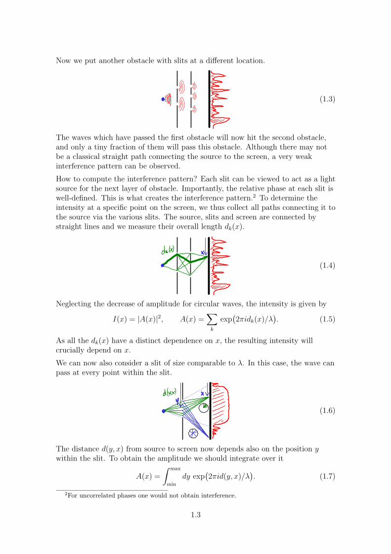
Now we put another obstacle with slits at a different location.

(1.3)

The waves which have passed the first obstacle will now hit the second obstacle,and only a tiny fraction of them will pass this obstacle. Although there may notbe a classical straight path connecting the source to the screen, a very weakinterference pattern can be observed.

How to compute the interference pattern? Each slit can be viewed to act as a lightsource for the next layer of obstacle. Importantly, the relative phase at each slit iswell-defined. This is what creates the interference pattern.2 To determine theintensity at a specific point on the screen, we thus collect all paths connecting it tothe source via the various slits. The source, slits and screen are connected bystraight lines and we measure their overall length dk(x).

(1.4)

Neglecting the decrease of amplitude for circular waves, the intensity is given by

I(x) = |A(x)|2, A(x) =∑k

exp(2πidk(x)/λ

). (1.5)

As all the dk(x) have a distinct dependence on x, the resulting intensity willcrucially depend on x.

We can now also consider a slit of size comparable to λ. In this case, the wave canpass at every point within the slit.

(1.6)

The distance d(y, x) from source to screen now depends also on the position ywithin the slit. To obtain the amplitude we should integrate over it

A(x) =

∫ max

min

dy exp(2πid(y, x)/λ

). (1.7)

2For uncorrelated phases one would not obtain interference.

1.3

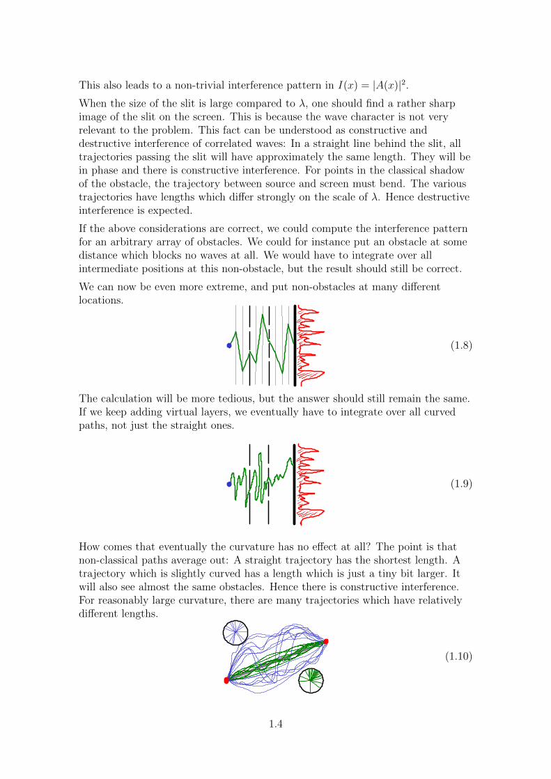
This also leads to a non-trivial interference pattern in I(x) = |A(x)|2.

When the size of the slit is large compared to λ, one should find a rather sharpimage of the slit on the screen. This is because the wave character is not veryrelevant to the problem. This fact can be understood as constructive anddestructive interference of correlated waves: In a straight line behind the slit, alltrajectories passing the slit will have approximately the same length. They will bein phase and there is constructive interference. For points in the classical shadowof the obstacle, the trajectory between source and screen must bend. The varioustrajectories have lengths which differ strongly on the scale of λ. Hence destructiveinterference is expected.

If the above considerations are correct, we could compute the interference patternfor an arbitrary array of obstacles. We could for instance put an obstacle at somedistance which blocks no waves at all. We would have to integrate over allintermediate positions at this non-obstacle, but the result should still be correct.

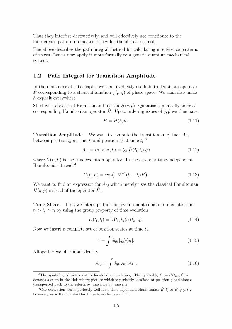
We can now be even more extreme, and put non-obstacles at many differentlocations.

(1.8)

The calculation will be more tedious, but the answer should still remain the same.If we keep adding virtual layers, we eventually have to integrate over all curvedpaths, not just the straight ones.

(1.9)

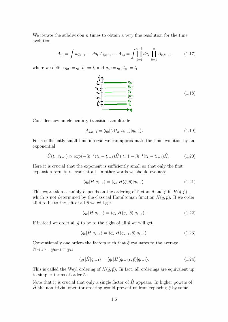
How comes that eventually the curvature has no effect at all? The point is thatnon-classical paths average out: A straight trajectory has the shortest length. Atrajectory which is slightly curved has a length which is just a tiny bit larger. Itwill also see almost the same obstacles. Hence there is constructive interference.For reasonably large curvature, there are many trajectories which have relativelydifferent lengths.

(1.10)

1.4

Thus they interfere destructively, and will effectively not contribute to theinterference pattern no matter if they hit the obstacle or not.

The above describes the path integral method for calculating interference patternsof waves. Let us now apply it more formally to a generic quantum mechanicalsystem.

1.2 Path Integral for Transition Amplitude

In the remainder of this chapter we shall explicitly use hats to denote an operatorF corresponding to a classical function f(p, q) of phase space. We shall also make~ explicit everywhere.

Start with a classical Hamiltonian function H(q, p). Quantise canonically to get acorresponding Hamiltonian operator H. Up to ordering issues of q, p we thus have

H = H(q, p). (1.11)

Transition Amplitude. We want to compute the transition amplitude Af,i

between position qi at time ti and position qf at time tf3

Af,i = 〈qf , tf |qi, ti〉 = 〈qf |U(tf , ti)|qi〉 (1.12)

where U(tf , ti) is the time evolution operator. In the case of a time-independentHamiltonian it reads4

U(tf , ti) = exp(−i~−1(tf − ti)H

). (1.13)

We want to find an expression for Af,i which merely uses the classical Hamiltonian

H(q, p) instead of the operator H.

Time Slices. First we interrupt the time evolution at some intermediate timetf > tk > ti by using the group property of time evolution

U(tf , ti) = U(tf , tk)U(tk, ti). (1.14)

Now we insert a complete set of position states at time tk

1 =

∫dqk |qk〉〈qk|. (1.15)

Altogether we obtain an identity

Af,i =

∫dqk Af,kAk,i. (1.16)

3The symbol |q〉 denotes a state localised at position q. The symbol |q, t〉 := U(tref , t)|q〉denotes a state in the Heisenberg picture which is perfectly localised at position q and time ttransported back to the reference time slice at time tref .

4Our derivation works perfectly well for a time-dependent Hamiltonian H(t) or H(q, p, t),however, we will not make this time-dependence explicit.

1.5

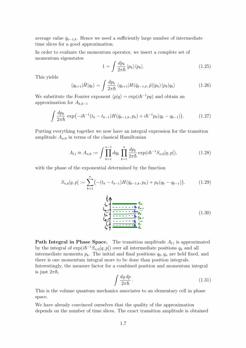
We iterate the subdivision n times to obtain a very fine resolution for the timeevolution

Af,i =

∫dqn−1 . . . dq1Af,n−1 . . . A1,i =

∫ n−1∏k=1

dqk

n∏k=1

Ak,k−1, (1.17)

where we define q0 := qi, t0 := ti and qn := qf , tn := tf .

(1.18)

Consider now an elementary transition amplitude

Ak,k−1 = 〈qk|U(tk, tk−1)|qk−1〉. (1.19)

For a sufficiently small time interval we can approximate the time evolution by anexponential

U(tk, tk−1) ' exp(−i~−1(tk − tk−1)H

)' 1− i~−1(tk − tk−1)H. (1.20)

Here it is crucial that the exponent is sufficiently small so that only the firstexpansion term is relevant at all. In other words we should evaluate

〈qk|H|qk−1〉 = 〈qk|H(q, p)|qk−1〉. (1.21)

This expression certainly depends on the ordering of factors q and p in H(q, p)which is not determined by the classical Hamiltonian function H(q, p). If we orderall q to be to the left of all p we will get

〈qk|H|qk−1〉 = 〈qk|H(qk, p)|qk−1〉. (1.22)

If instead we order all q to be to the right of all p we will get

〈qk|H|qk−1〉 = 〈qk|H(qk−1, p)|qk−1〉. (1.23)

Conventionally one orders the factors such that q evaluates to the averageqk−1,k := 1

2qk−1 + 1

2qk

〈qk|H|qk−1〉 = 〈qk|H(qk−1,k, p)|qk−1〉. (1.24)

This is called the Weyl ordering of H(q, p). In fact, all orderings are equivalent upto simpler terms of order ~.

Note that it is crucial that only a single factor of H appears. In higher powers ofH the non-trivial operator ordering would prevent us from replacing q by some

1.6

average value qk−1,k. Hence we need a sufficiently large number of intermediatetime slices for a good approximation.

In order to evaluate the momentum operator, we insert a complete set ofmomentum eigenstates

1 =

∫dpk2π~|pk〉〈pk|. (1.25)

This yields

〈qk+1|H|qk〉 =

∫dpk2π~〈qk+1|H(qk−1,k, p)|pk〉〈pk|qk〉 (1.26)

We substitute the Fourier exponent 〈p|q〉 = exp(i~−1pq) and obtain anapproximation for Ak,k−1∫

dpk2π~

exp(−i~−1(tk − tk−1)H(qk−1,k, pk) + i~−1pk(qk − qk−1)

). (1.27)

Putting everything together we now have an integral expression for the transitionamplitude An,0 in terms of the classical Hamiltonian

Af,i ≈ An,0 :=

∫ n−1∏k=1

dqk

n∏k=1

dpk2π~

exp(i~−1Sn,0[q, p]), (1.28)

with the phase of the exponential determined by the function

Sn,0[q, p] :=n∑k=1

(−(tk − tk−1)H(qk−1,k, pk) + pk(qk − qk−1)

). (1.29)

(1.30)

Path Integral in Phase Space. The transition amplitude Af,i is approximatedby the integral of exp(i~−1Sn,0[q, p]) over all intermediate positions qk and allintermediate momenta pk. The initial and final positions q0, qn are held fixed, andthere is one momentum integral more to be done than position integrals.Interestingly, the measure factor for a combined position and momentum integralis just 2π~, ∫

dq dp

2π~. (1.31)

This is the volume quantum mechanics associates to an elementary cell in phasespace.

We have already convinced ourselves that the quality of the approximationdepends on the number of time slices. The exact transition amplitude is obtained

1.7

by formally taking the limit of infinitely many time slices at infinitesimal intervals.We abbreviate the limit by the so-called path integral

Af,i =

∫DqDp exp(i~−1Sf,i[q, p]), (1.32)

where the phase is now given as a functional of the path

Sf,i[q, p] =

∫ tf

ti

dt(p(t)q(t)−H(q(t), p(t))

)=

∫ f

i

(pdq −Hdt) . (1.33)

This path integral “integrates” over all paths (q(t), p(t)).

Comparing to the above discrete version, the term dt pq ≈ pk(qk − qk−1) isresponsible for shifting the time slice forward, whereas the Hamiltonian governsthe evolution of the wave function.

The expression we obtained for the phase factor Sf,i[q, p] is exciting, it is preciselythe action in phase space. Note that the associated Euler–Lagrange equations

0 =δS

δq(t)= −p(t)− ∂H

∂q(t) , 0 =

δS

δp(t)= +q(t)− ∂H

∂p(t) , (1.34)

are just the Hamiltonian equations of motion.

Here the principle of extremal action for a classical path finds a justification: Theaction determines a complex phase Sf,i[q, p]/~ for each path (q(t), p(t)) in phasespace. Unless the action is extremal, the phase will vary substantially from onepath to a neighbouring one. On average such paths will cancel out from the pathintegral. Conversely, a path which extremises the action, has a stationary actionfor all neighbouring paths. These paths will dominate the path integral classically.When quantum corrections are taking into account, the allowable paths can wigglearound the classical trajectory slightly, on the order of ~.

The path integral for the transition amplitude Af,i, keeps the initial and finalpositions fixed

q(ti) = qi, q(tf) = qf , (1.35)

whereas the momenta p(ti) and p(tf) are free. The path integral can also computeother quantities where the boundary conditions are specified differently.

Note that the integration measures Dq and Dp typically hide some factors whichare hard to express explicitly. Usually such factors can be ignored during acalculation, and are only reproduced in the end by demanding appropriatenormalisation.

Finally, we must point out that the path integral may not be well-defined in amathematical sense, especially because the integrand is highly oscillating.Nevertheless, it is reasonably safe to use the path integral in physics by formallymanipulating it by the usual rules and inserting suitable regulators such as ±iε.

Path Integral in Position Space. The above path integral is based on theHamiltonian formulation where time has a distinguished role. For common

1.8

physical systems we can transform the path integral back to the originalLagrangian framework.

We merely need to assume that the Hamiltonian is quadratic in the momenta p

H(q, p) =p2

2M(q)+ pK(q) + V (q). (1.36)

For common physical models this is the case. For example, a classical particle ofmass m in a potential V (q) would have M(q) = m and K(q) = 0.

Notice that the exponent depends at most quadratically on each momentum. Thisallows to integrate all momenta out using the Gaussian integral5∫ +∞

−∞dp exp

(−1

2ap2 + bp+ c

)=√

2π/a exp(b2/2a+ c). (1.37)

We obtain an expression for the transition amplitude

An,0 =

∫ n−1∏k=1

dqk

n∏k=1

√M(qk−1,k)

2π~i(tk − tk−1)exp(i~−1Sn,0[q]), (1.38)

which depends on

Sn,0[q] =n∑k=1

(tk − tk−1)

[− V (qk−1,k)

+ 12M(qk−1,k)

(qk − qk−1

tk − tk−1

−K(qk−1,k)

)2 ]. (1.39)

Now the exact path integral for the transition amplitude reads

Af,i =

∫Dq exp(i~−1Sf,i[q]), (1.40)

where the phase is given by the conventional action for a particle

Sf,i[q] =

∫ n

0

dt(

12M(q)(q −K(q))2 − V (q)

). (1.41)

Evidently, this action is classically equivalent to the above action in Hamiltonianform. Here we see that both classical actions yield the same path integral, and aretherefore quantum equivalent. This is a special case, and quantum equivalence isnot to be expected for two equivalent classical actions.

Note that the measure factor hidden in Dq is substantially more complicatedcompared to the combination DqDp. In fact, it depends on the mass term M(q).For a standard classical particle M(q) = m is independent of q and hence theintegration measure amounts to some constant overall factor.

5The formula is applicable as long as a has a positive real part, however small it may be. Inour case, a is purely imaginary, but by the usual assumptions of causality allow to attribute asmall real positive part to a.

1.9

We have finally obtained an expression for the quantum transition amplitude Af,i

which is based just on the classical action in the Lagrangian formulation. There isno need to translate to the Hamiltonian framework at any point of the calculation.In fact, we can generally use the path integral to define transition amplitudes orother quantum mechanical expressions. Note that the precise discretisation of theaction S[q], i.e. how to represent each instance of q(t) and q(t), can influence thevalue of the path integral. This effect is equivalent to the choice of operatororderings. We will discuss these ambiguities further below.

1.3 Free Particle

Let us discuss a simple example, the free non-relativistic particle. We have derivedtwo expressions for the path integral.

Phase Space. The free particles is defined by the Hamiltonian

H(q, p) =p2

2m. (1.42)

The discretised action in phase space therefore reads

Sn,0[q, p] :=n∑k=1

(−(tk − tk−1)p2

k/2m+ pk(qk − qk−1)). (1.43)

We observe that each variable qk appears only in a product with either pk or pk+1.The integral over qk therefore yields the delta-function δ(pk+1 − pk) whichtrivialises one of the momentum integrals. Altogether we find

An,0 =

∫ n−1∏k=1

dqk

n∏k=1

dpk2π~

exp(i~−1Sn,0[q, p]),

=

∫dp

2π~exp(i~−1

(−(tn − t0)p2/2m+ p(qn − q0)

))=

√m

2π~i(tn − t0)exp

(im(qn − q0)2

2~(tn − t0)

). (1.44)

This is the correct transition amplitude Af,i for a free non-relativistic particle.Actually the number of intermediate steps n does not matter here because of thesimplicity of the problem; usually the limit n→∞ is required.

Position Space. Alternatively, we can start with the classical discretised action

Sn,0[q] = 12m

n∑k=1

(qk − qk−1)2

tk − tk−1

. (1.45)

It turns out that every integral over a qk in

An,0 =

∫ n−1∏k=1

dqk

n∏k=1

√m

2π~i(tk − tk−1)exp(i~−1Sn,0[q]), (1.46)

1.10

simply eliminates the set of variables (qk, tk) from their sequences without leavinga gap in the above expression. Eventually, we thus find

An,0 =

√m

2π~i(tn − t0)exp

(im(qn − q0)2

2~(tn − t0)

). (1.47)

Gladly the two results agree.

1.4 Operator Insertions

We have found a way to express the transition amplitude 〈qf , tf |qi, ti〉 in terms of apath integral.

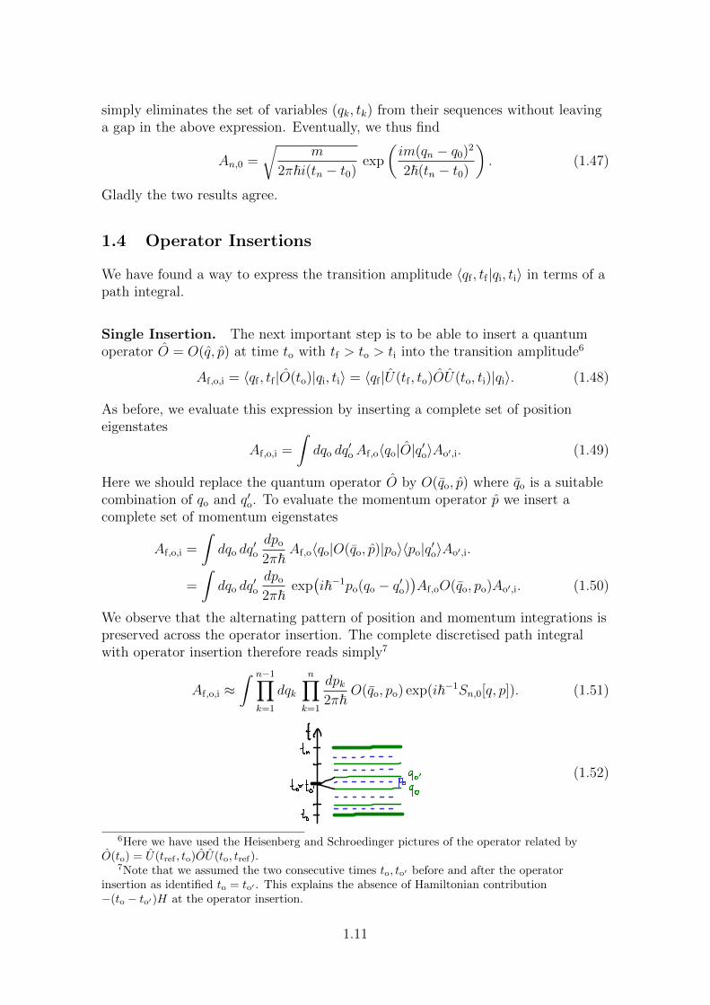
Single Insertion. The next important step is to be able to insert a quantumoperator O = O(q, p) at time to with tf > to > ti into the transition amplitude6

Af,o,i = 〈qf , tf |O(to)|qi, ti〉 = 〈qf |U(tf , to)OU(to, ti)|qi〉. (1.48)

As before, we evaluate this expression by inserting a complete set of positioneigenstates

Af,o,i =

∫dqo dq

′oAf,o〈qo|O|q′o〉Ao′,i. (1.49)

Here we should replace the quantum operator O by O(qo, p) where qo is a suitablecombination of qo and q′o. To evaluate the momentum operator p we insert acomplete set of momentum eigenstates

Af,o,i =

∫dqo dq

′o

dpo

2π~Af,o〈qo|O(qo, p)|po〉〈po|q′o〉Ao′,i.

=

∫dqo dq

′o

dpo

2π~exp(i~−1po(qo − q′o)

)Af,oO(qo, po)Ao′,i. (1.50)

We observe that the alternating pattern of position and momentum integrations ispreserved across the operator insertion. The complete discretised path integralwith operator insertion therefore reads simply7

Af,o,i ≈∫ n−1∏

k=1

dqk

n∏k=1

dpk2π~

O(qo, po) exp(i~−1Sn,0[q, p]). (1.51)

(1.52)

6Here we have used the Heisenberg and Schroedinger pictures of the operator related byO(to) = U(tref , to)OU(to, tref).

7Note that we assumed the two consecutive times to, to′ before and after the operatorinsertion as identified to = to′ . This explains the absence of Hamiltonian contribution−(to − to′)H at the operator insertion.

1.11

As a continuous path integral it takes the form

Af,o,i =

∫DqDpO(q(to), p(to)) exp(i~−1Sf,i[q, p]). (1.53)

Time Ordering. It should now be evident how to insert multiple operators intothe path integral. Suppose we have n operators Ok at times tk, respectively, withtf > tn > . . . > t2 > t1 > ti. We insert them into the transition amplitude andobtain a path integral with n operator insertions

〈qf , tf |On . . . O2O1|qi, ti〉.

=

∫DqDpO1(t1)O2(t2) . . . On(tn) exp(i~−1Sf,i[q, p]). (1.54)

It is crucial that all the operators are in proper time order. Only then all the timeevolution operators U(tk, tk−1) will shift time forward as in the above derivation ofthe path integral.

Conversely, a set of operators insertions in the path integral corresponds to atime-ordered product of quantum operators inserted into the transition amplitude∫

DqDp

n∏k=1

Ok(tk) exp(i~−1Sf,i[q, p]).

= 〈qf , tf |T(O1O2 . . . On)|qi, ti〉. (1.55)

This relation holds even for an arbitrary ordering of operator times tk. Hence thepath integral performs time-ordering automatically.8

In some sense, the time ordering enters by the very definition of the path integral:There is precisely one position for each time, the trajectory strictly moves forwardin time, there cannot be loops in time. This ordering of times is forced upon theoperator insertions.

Equal-Time Commutators. The strict built-in ordering of times makescommutation relations between the operators irrelevant. The only operator algebrawe can possibly consider is at equal times. Let us therefore understand how torealise the fundamental commutation relation

[q, p] = i~. (1.56)

We would like to insert the operator O = [q, p] into the path integral.Unfortunately, there is no classical equivalent O(q, p) to O except for the numberi~, but that would amount to postulation rather than derivation.

The trick is to separate the times slightly:9

O(t) = q(t)p(t− ε)− p(t+ ε)q(t). (1.57)

8To compute expectation values of quantum operators which are not in proper time orderwith the path integral is more laborious, but could be handled manually.

9In fact, the product q(t)p(t) at equal times is ill-defined in the continuous path integral sincethe insertion q(t)p(t+ δt) is discontinuous at δt = 0 (by precisely i~).

1.12

The intrinsic time ordering then puts the operators into their desired order. Infact, the discretised path integral knows about the ordering problem and does noteven permit ambiguous orderings of positions and momenta: The positionvariables qk were defined at times tk. The associated momenta pk, however, are notlocated at tk, but rather between tk and tk−1. This fact is most evident in theexpression for the discretised action

Sn,0[q, p] :=n∑k=1

(−(tk − tk−1)H(qk−1,k, pk) + pk(qk − qk−1)

). (1.58)

The above operator is therefore discretised as follows

O = qkpk − pk+1qk. (1.59)

We insert the operator into the discretised path integral for the transitionamplitude 〈qf , tf |O|qi, ti〉 of free non-relativistic particle. We can perform mostintegrations trivially as before∫

dpk2π~

dqkdpk+1

2π~qk(pk − pk+1)

· exp(− i

2~−1m−1

((tn − tk)p2

k+1 + (tk − t0)p2k

))· exp

(i~−1(pk+1qn − pkq0)

)exp(i~−1(pk − pk+1)qk

). (1.60)

We then convert the factor qk to a differential operator acting on the latterexponent, and perform the integral over qk as a delta function∫

dpk2π~

dpk+1 (pk − pk+1)

· exp(− i

2~−1m−1

((tn − tk)p2

k+1 + (tk − t0)p2k

))· exp

(i~−1(pk+1qn − pkq0)

)(−i~ ∂

∂pkδ(pk+1 − pk)

). (1.61)

Now the only thing that protects the factor (pk − pk−1) from vanishing by means ofthe delta function δ(pk − pk−1) is the derivative ∂/∂pk. We therefore perform apartial integration and let the derivative act on the remainder of the integrand.Unless it hits the factor (pk − pk−1), the integral must vanish, hence∫

dpk2π~

dpk+1 δ(pk+1 − pk)(i~

∂

∂pk(pk − pk+1)

)· exp

(i~−1

(−(tn − t0)p2

k/2m+ pk(qn − q0)))

= i~∫

dp

2π~exp(i~−1

(−(tn − t0)p2/2m+ p(qn − q0)

)). (1.62)

This is precisely i~ times the transition amplitude An,0. Hence we learn from thepath integral that

〈qf , tf |[q, p]|qi, ti〉 = i~〈qf , tf |qi, ti〉, (1.63)

which is fully consistent with canonical quantisation.

1.13

This result shows (once again) that quantisation of a classical operator O(q, p)depends crucially on the discretisation O(qk−1,k, pk). The precise choice of qk−1,k,whether to use qk−1, qk, their arithmetic mean or something else, has a similareffect as operator ordering in the canonical framework. However, since thecanonical commutator [q, p] = i~ is simple enough, one can always add appropriateterms of O(~) to O(q, p) to make any given discretisation O(qk−1,k, pk) correspond

to the desired quantum operator O.

1.14

Quantum Field Theory II Chapter 2ETH Zurich, FS13 Prof. N. Beisert

22. 10. 2014

2 Path Integral for Fields

2.1 Time-Ordered Correlators

We know how to express a quantum mechanical transition amplitude with the pathintegral. This generalises straight-forwardly to fields (we set ~ = 1 for convenience)

〈Ψf , tf |T(O1 . . . On)|Ψi, ti〉

=

∫DΨ O1[Ψ ] . . . On[Ψ ] exp(iSf,i[Ψ ]). (2.1)

Here Ψi,f are the spatial fields at the initial and final time slices, whereas Ψ is afield in spacetime which interpolates between the fields Ψi = Ψ(ti) and Ψf = Ψ(tf).The action can be written as an integral over the Lagrangian (density)

Sf,i[Ψ ] :=

∫ tf

ti

dt L[Ψ(t)] =

∫ f

i

dDxL(Ψ(x), ∂µΨ(x)). (2.2)

This expression is almost covariant, but it still makes reference to two particulartime slices. Moreover, we are usually not so much interested in transitionamplitudes between particular field configurations, but rather in time-orderedcorrelators

〈O1 . . . On〉 := 〈0|T(O1 . . . On)|0〉. (2.3)

To solve these problems, we can apply a trick we have learned in QFT I: A genericstate such as |Ψi, ti〉 can be expected to have some overlap with the ground state|0〉. Letting the state evolve for some time while adding some friction (let the timehave a small imaginary component) makes the state decay to its lowest-energycontribution, i.e. the ground state.

We therefore take the limit tf,i → ±∞(1− iε) and obtain a familiar expression forthe time-order correlator

〈O1 . . . On〉 =

∫DΨ O1[Ψ ] . . . On[Ψ ] exp(iS[Ψ ])∫

DΨ exp(iS[Ψ ]). (2.4)

Here the path integrals integrate over fields Ψ defined for all of spacetime, and theaction is the integral of the Lagrangian density over all of spacetime

S[Ψ ] =

∫dDxL(Ψ(x), ∂µΨ(x)). (2.5)

The term in the denominator accounts for the overlap of the initial and final stateswith the ground state. It evidently takes care of proper normalisation 〈1〉 = 1.

2.1

Even more, it conveniently eliminates any constant factor in the integrationmeasure DΨ allowing us to be somewhat sloppy in defining the latter.

As discussed in QFT I, the slight tilting of the time axis into the complex planeselects Feynman propagators as Green functions. When we keep this in mind, wedo not to consider the tilting anymore. The path integral expression fortime-ordered1 time-ordered correlators is thus perfectly relativistic.

The main application of the path integral in quantum field theory is to computetime-ordered vacuum expectation values. It may also be used to compute differentquantities by specifying alternative boundary conditions for the integration overfields Ψ .

2.2 Sources and Generating Functional

In principle, we can now compute correlators such as

〈Ψ(x)Ψ(y)〉 =

∫DΨ Ψ(x)Ψ(y) exp(iS[Ψ ])∫

DΨ exp(iS[Ψ ]). (2.6)

In a free theory it amounts to a Gaussian integral with prefactors. The evaluationis complicated by the fact that derivatives of Ψ appear in the action, and it is notimmediately clear how to apply the standard methods to put additional factorsfrom of the Gaussian exponent. Therefore, the integral should be discretised whichoften leads to a involved combinatorics.

Sources. Gladly there is a standard trick to insert factors in front of theexponential factor using source terms. We define the generating functional Z[J ]

Z[J ] :=

∫DΨ exp

(iS[Ψ ] + iSsrc[Ψ, J ]

)(2.7)

as a standard path integral but with an additional source term in the action2

Ssrc[Ψ, J ] :=

∫dDxΨ(x)J(x). (2.8)

This source term has the simple property that a functional derivative w.r.t. thesource J(x) produces precisely the field Ψ(x) at the same location

δSsrc[Ψ, J ]

δJ(x)=

∫dDy Ψ(y)δD(x− y) = Ψ(x). (2.9)

When the source action is in the exponent, the functional derivative brings downone power of Ψ without altering the exponent

−iδδJ(x)

exp(iSsrc[Ψ, J ]

)= Ψ(x) exp

(iSsrc[Ψ, J ]

). (2.10)

1Here time ordering can be interpreted as causality since fields commute outside the light-cone.2The field J(x) is the same source field as discussed in QFT I in connection to propagators.

2.2

Moreover, the source field does not appear in the original action. Hence, functionalderivatives of Z[J ] w.r.t. the source insert factors of Ψ(x) into the path integral

Ψ(x) ' −iδδJ(x)

. (2.11)

For example, we express two insertions as a double functional derivative of Z[J ]

−iδδJ(x)

−iδδJ(y)

Z[J ] =

∫DΨ Ψ(x)Ψ(y) exp(iS[Ψ ] + iSsrc[Ψ, J ]). (2.12)

Now we still need to get rid of the source term in the exponent by setting J = 0.The time-ordered two-point correlator with proper normalisation term finally takesthe form

〈Ψ(x)Ψ(y)〉 = Z[J ]−1 −iδδJ(x)

−iδδJ(y)

Z[J ]

∣∣∣∣J=0

. (2.13)

Free Scalar Field. Now we can formally write any time-ordered correlators, buthow to compute them in practice? We can only expect to obtain an exactexpression for free fields. Therefore consider the scalar field. The action withsource term reads

S[φ] + Ssrc[φ, j] =

∫dDx

(−1

2(∂φ)2 − 1

2m2φ2 + jφ

). (2.14)

By partial integration we can make all the derivatives act on a single field

S[φ] + Ssrc[φ, j] =

∫dDx

(12φ(∂2 −m2)φ+ φj

). (2.15)

This is a Gaussian integral can be performed by shifting the integration variable φ.A complication is that the kernel of the Gaussian function is the derivativeoperator (−∂2 +m2), and result of the integral depends on its inverse. We havealready determined its inverse in QFT I, it is the propagator GF(x− y) satisfying3

(−∂2 +m2)GF(x− y) = δD(x− y). (2.16)

Hence we shift the field

φ(x) = φ(x) +

∫dDy GF(x− y)j(y). (2.17)

and substitute it into the action

S[φ] + Ssrc[φ, j] =

∫dDx 1

2φ(x)(∂2 −m2)φ(x) +W [j].

W [j] =

∫dDx dDy 1

2j(x)GF(x− y)j(y). (2.18)

3Due to the tilting of the time axis into the complex plane, we have to choose the Feynmanpropagator.

2.3

As φ and j are now well-separated, we can now perform the integral over φ.Moreover, the integration measure does not change Dφ = Dφ when the integrationvariable is shifted. Up to the overall constant Z[0] we thus get

Z[j] = Z[0] exp(iW [j]

). (2.19)

A derivation in momentum space is somewhat simpler because the Gaussian kernelis automatically diagonal. The momentum-space version of W [j] is4

W [j] =

∫dDp

12j(p)j(−p)

p2 +m2 − iε=

∫dDp

12|j(p)|2

p2 +m2 − iε. (2.20)

Formally, the prefactor reads5

Z[0] ∼ 1√det(−∂2 +m2 − iε)

. (2.21)

Wick’s Theorem. Let us now compute 〈Ψ(x)Ψ(y)〉. We perform two functionalderivatives6

−iδδJ(y)

−iδδJ(x)

Z[J ]

=−iδδJ(y)

∫dDz GF(x− z)J(z)Z[J ]

= − iGF(x− y)Z[J ]

+

∫dDz dDz′GF(x− z)J(z)GF(y − z′)J(z′)Z[J ] . (2.22)

Now divide by Z[J ] and set J = 0 to obtain the correlator

〈φ(x)φ(y)〉 = −iGF(x− y). (2.23)

This is precisely the expected result.

We can also perform the exercise with more than two fields. The result agrees withWick’s theorem. In fact the form of Z[J ] as the exponent of W [J ] which is aquadratic monomial of J can be viewed as the functional formulation of Wick’stheorem:

• The first derivative knocks down a linear term δW/δJ from the quadraticexponent.• Subsequent derivatives can knock further linear terms δW/δJ from the

exponent. They can also hit the remaining J in some δW/δJ leaving behind aFeynman propagator −iGF(xk − xl).4The factor of 1/2 compensates the double-counting of |j(p)| = |j(−p)|.5This statement is more or less tautological in QFT since the determinant of an operator is

commonly defined via a Gaussian integral. Here, Z[0] is a constant (independent of the otherfields) and can therefore be ignored.

6There are two equivalent factors of J in the exponent of Z[J ], so the functional derivativeacting on them produces a factor of 2 to be cancelled by the prefactor of 1/2.

2.4

• Any linear term δW/δJ that remains after the functional derivatives cause theexpression to vanish when J = 0.• As every exponent requires two functional derivatives, all fields φ(xk) must be

Wick contracted to some other field.• The product rule of derivatives take care of the sum of all combinations.• Setting J = 0 in the end corresponds to the time-ordered correlator; it removes

all non-trivial normal ordered terms.

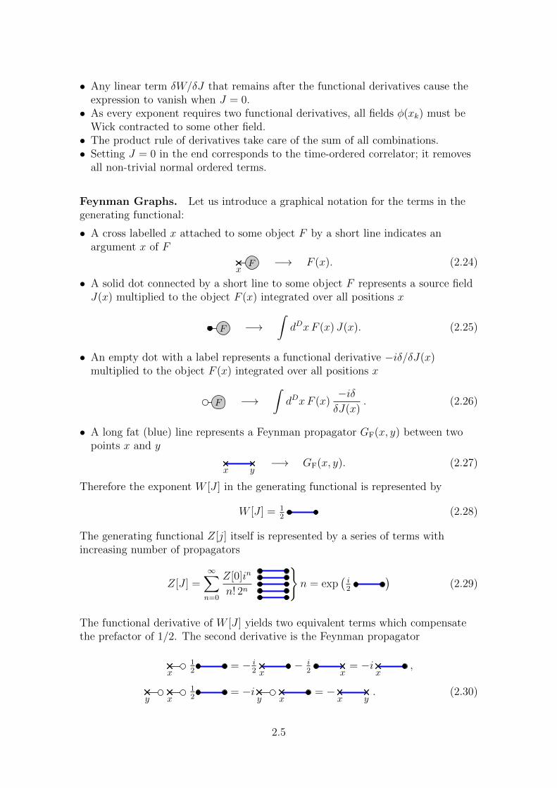
Feynman Graphs. Let us introduce a graphical notation for the terms in thegenerating functional:

• A cross labelled x attached to some object F by a short line indicates anargument x of F

xF −→ F (x). (2.24)

• A solid dot connected by a short line to some object F represents a source fieldJ(x) multiplied to the object F (x) integrated over all positions x

F −→∫dDxF (x) J(x). (2.25)

• An empty dot with a label represents a functional derivative −iδ/δJ(x)multiplied to the object F (x) integrated over all positions x

F −→∫dDxF (x)

−iδδJ(x)

. (2.26)

• A long fat (blue) line represents a Feynman propagator GF(x, y) between twopoints x and y

x y−→ GF(x, y). (2.27)

Therefore the exponent W [J ] in the generating functional is represented by

W [J ] = 12

(2.28)

The generating functional Z[j] itself is represented by a series of terms withincreasing number of propagators

Z[J ] =∞∑n=0

Z[0]in

n! 2n

n = exp

(i2

)(2.29)

The functional derivative of W [J ] yields two equivalent terms which compensatethe prefactor of 1/2. The second derivative is the Feynman propagator

x12

= − i2 x

− i2 x

= −ix

,

y x12

= −iy x

= −x y

. (2.30)

2.5

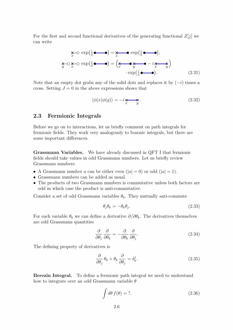
For the first and second functional derivatives of the generating functional Z[j] wecan write

xexp(i2

)=x

exp(i2

),

y xexp(i2

)=(x y

− ix y

)· exp

(i2

). (2.31)

Note that an empty dot grabs any of the solid dots and replaces it by (−i) times across. Setting J = 0 in the above expressions shows that

〈φ(x)φ(y)〉 = −ix y

. (2.32)

2.3 Fermionic Integrals

Before we go on to interactions, let us briefly comment on path integrals forfermionic fields. They work very analogously to bosonic integrals, but there aresome important differences.

Grassmann Variables. We have already discussed in QFT I that fermionicfields should take values in odd Grassmann numbers. Let us briefly reviewGrassmann numbers:

• A Grassmann number a can be either even (|a| = 0) or odd (|a| = 1).• Grassmann numbers can be added as usual.• The products of two Grassmann numbers is commutative unless both factors are

odd in which case the product is anti-commutative.

Consider a set of odd Grassmann variables θk. They mutually anti-commute

θjθk = −θkθj. (2.33)

For each variable θk we can define a derivative ∂/∂θk. The derivatives themselvesare odd Grassmann quantities

∂

∂θj

∂

∂θk= − ∂

∂θk

∂

∂θj. (2.34)

The defining property of derivatives is

∂

∂θjθk + θk

∂

∂θj= δjk. (2.35)

Berezin Integral. To define a fermionic path integral we need to understandhow to integrate over an odd Grassmann variable θ∫

dθ f(θ) = ?. (2.36)

2.6

It makes sense to demand that the integral of a total derivative vanishes∫dθ

∂

∂θf(θ) = 0. (2.37)

Now due to anti-commutativity θ2 = 0 and hence a generic function f(θ) can beexpanded as f(θ) = f0 + θf1 with two coefficient f0 and f1. We substitute this intothe integral of a total derivative

0 =

∫dθ

∂

∂θ(f0 + θf1) =

∫dθ f1. (2.38)

It tells us that the integral of a constant must vanish. We can now integrate ageneric function ∫

dθ (f0 + θf1) =

(∫dθ θ

)f1. (2.39)

The integral∫dθ θ is some undetermined factor, we can define it as 1. The curious

result is that integration of odd Grassmann variables is equivalent todifferentiation7 ∫

dθ f(θ) =∂

∂θf(θ). (2.40)

The so-called Berezin integral over odd Grassmann variables behaves in manyother respects like the standard bosonic integral. For the path integral in quantumfield theory, the most important issues are Fourier integrals, delta functions andGaussian integrals. Let us consider these now:

Delta Functions. We can convince ourselves that the defining property of thedelta function ∫

dθ δ(θ − α)f(θ) = f(α) (2.41)

is solved trivially by8

δ(θ) = θ. (2.42)

Under variable transformations this delta function behaves as

δ(φ(θ)) =∂φ

∂θδ(θ − θ0). (2.43)

This is analogous to the transformation of the bosonic delta function except thatthe Jacobian of the transformation multiplies the delta function (and no absolutevalues are taken).

Fourier Integrals. A plain Fourier integral produces a delta function as usual∫dθ exp(cθα) =

∫dθ(1 + cθα

)= cα = cδ(α). (2.44)

Note that the coefficient c of the exponent can be an arbitrary (Grassmann even)number.

7This implies that the integration measure dθ has the dimension of ∂/∂θ or 1/θ.8Note that the order of terms in δ(θ − α) does matter since δ(α− θ) = −δ(θ − α).

2.7

Gaussian Integrals. To define a Gaussian integral, we need at least twoGrassmann odd variables, otherwise the quadratic exponent would vanish byconstruction. For the simplest Gaussian integral we obtain∫

dθ2 dθ1 exp(aθ1θ2) = a. (2.45)

To make this more reminiscent of a usual n-dimensional Gaussian integral let usintroduce a 2× 2 matrix A

A =

(0 +a−a 0

). (2.46)

The result can be expressed as∫dnθ exp(1

2θTAθ) ∼

√det(A) . (2.47)

This result in fact applies to general fermionic Gaussian integrals defined in termsof an n× n anti-symmetric matrix A.9 This expression is very similar to thebosonic n-dimensional Gaussian integral for a symmetric matrix S∫

dnx exp(−12xTSx) ∼ 1√

det(S). (2.48)

The crucial difference is that the determinant of the matrix appears with positiverather than negative exponent. Moreover, the matrix A does not need to fulfil anypositivity requirements since the odd integral is always well-defined.

Complex Gaussian Integrals. For complex fields one usually encounterscomplex Gaussian integrals. One may decompose them into real Gaussian integralsof twice the dimension. For a odd integration variables one finds∫

dnθ dnθ exp(θMθ) ∼ det(M), (2.49)

whereas the corresponding integral for even variables reads∫dnx dnx exp(−xMx) ∼ 1

det(M), (2.50)

In the latter bosonic case, the matrix M should obey some positivity constraints tomake the integral convergent, whereas the fermionic integral is indifferent to thesignature of M .

Summary. Altogether, when dealing with bosonic and fermionic fields we mustpay attention to

• the ordering of fields (and pick up appropriate sign factors for reordering),• the ordering of derivatives and integration measures,• the exponents of factors associated to integrals.

Otherwise the procedures are much the same. For example, completion of a squareis the essential step to solve Gaussian integrals for free fields.

9A fermionic Gaussian integral requires an even number of integration variables n because thedeterminant of an odd-dimensional anti-symmetric matrix is zero.

2.8

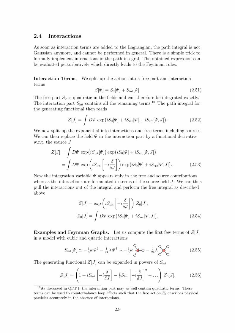
2.4 Interactions

As soon as interaction terms are added to the Lagrangian, the path integral is notGaussian anymore, and cannot be performed in general. There is a simple trick toformally implement interactions in the path integral. The obtained expression canbe evaluated perturbatively which directly leads to the Feynman rules.

Interaction Terms. We split up the action into a free part and interactionterms

S[Ψ ] = S0[Ψ ] + Sint[Ψ ]. (2.51)

The free part S0 is quadratic in the fields and can therefore be integrated exactly.The interaction part Sint contains all the remaining terms.10 The path integral forthe generating functional then reads

Z[J ] =

∫DΨ exp

(iS0[Ψ ] + iSint[Ψ ] + iSsrc[Ψ, J ]

). (2.52)

We now split up the exponential into interactions and free terms including sources.We can then replace the field Ψ in the interaction part by a functional derivativew.r.t. the source J

Z[J ] =

∫DΨ exp

(iSint[Ψ ]

)exp(iS0[Ψ ] + iSsrc[Ψ, J ]

)=

∫DΨ exp

(iSint

[−i δδJ

])exp(iS0[Ψ ] + iSsrc[Ψ, J ]

). (2.53)

Now the integration variable Ψ appears only in the free and source contributionswhereas the interactions are formulated in terms of the source field J . We can thuspull the interactions out of the integral and perform the free integral as describedabove

Z[J ] = exp

(iSint

[−i δδJ

])Z0[J ],

Z0[J ] =

∫DΨ exp

(iS0[Ψ ] + iSsrc[Ψ, J ]

). (2.54)

Examples and Feynman Graphs. Let us compute the first few terms of Z[J ]in a model with cubic and quartic interactions

Sint[Ψ ] ' −16κΨ 3 − 1

24λΨ 4 ∼ −1

6κ − 1

24λ . (2.55)

The generating functional Z[J ] can be expanded in powers of Sint

Z[J ] =

(1 + iSint

[−i δδJ

]− 1

2Sint

[−i δδJ

]2

+ . . .

)Z0[J ]. (2.56)

10As discussed in QFT I, the interaction part may as well contain quadratic terms. Theseterms can be used to counterbalance loop effects such that the free action S0 describes physicalparticles accurately in the absence of interactions.

2.9

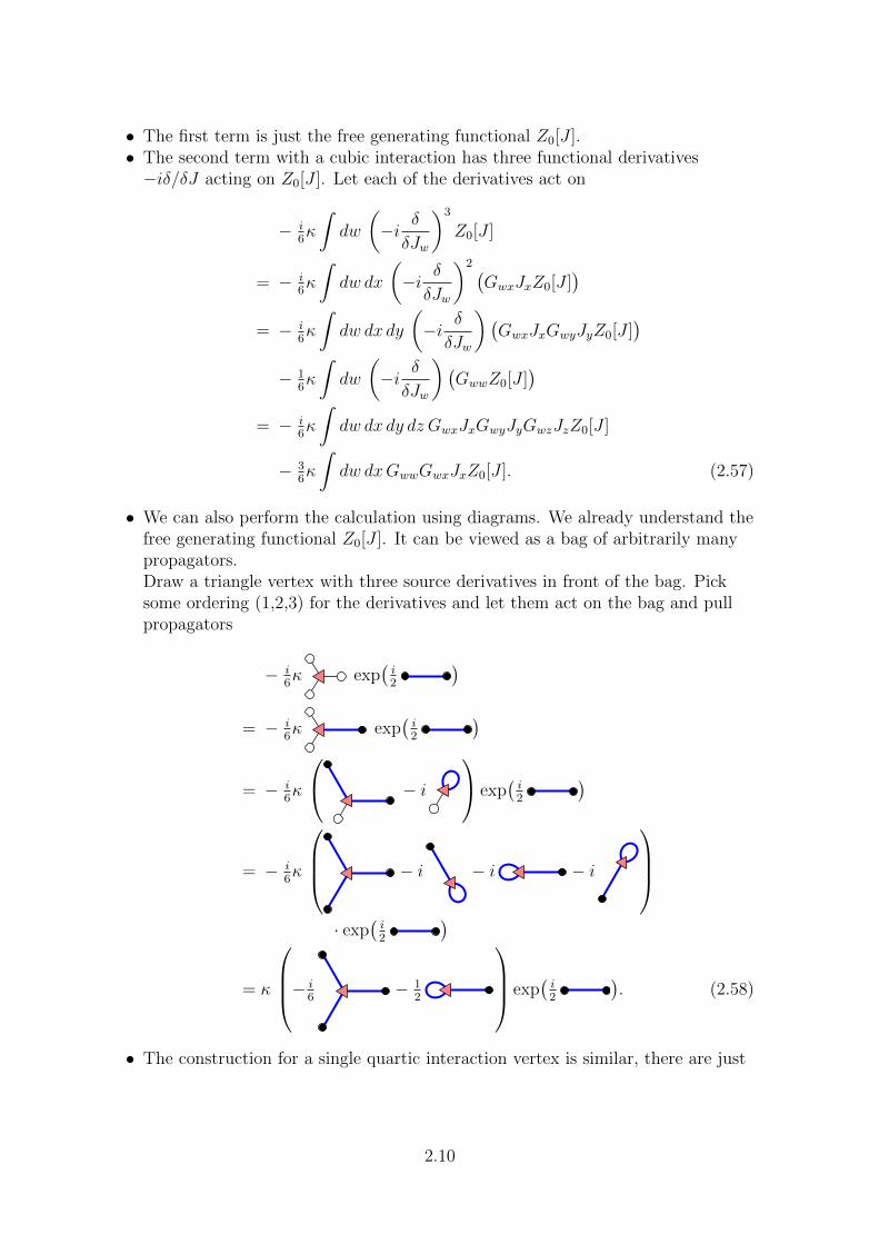
• The first term is just the free generating functional Z0[J ].• The second term with a cubic interaction has three functional derivatives−iδ/δJ acting on Z0[J ]. Let each of the derivatives act on

− i6κ

∫dw

(−i δ

δJw

)3

Z0[J ]

= − i6κ

∫dw dx

(−i δ

δJw

)2 (GwxJxZ0[J ]

)= − i

6κ

∫dw dx dy

(−i δ

δJw

)(GwxJxGwyJyZ0[J ]

)− 1

6κ

∫dw

(−i δ

δJw

)(GwwZ0[J ]

)= − i

6κ

∫dw dx dy dz GwxJxGwyJyGwzJzZ0[J ]

− 36κ

∫dw dxGwwGwxJxZ0[J ]. (2.57)

• We can also perform the calculation using diagrams. We already understand thefree generating functional Z0[J ]. It can be viewed as a bag of arbitrarily manypropagators.Draw a triangle vertex with three source derivatives in front of the bag. Picksome ordering (1,2,3) for the derivatives and let them act on the bag and pullpropagators

− i6κ exp

(i2

)= − i

6κ exp

(i2

)= − i

6κ

− i

exp(i2

)

= − i6κ

− i − i − i

· exp

(i2

)= κ

− i6

− 12

exp(i2

). (2.58)

• The construction for a single quartic interaction vertex is similar, there are just

2.10

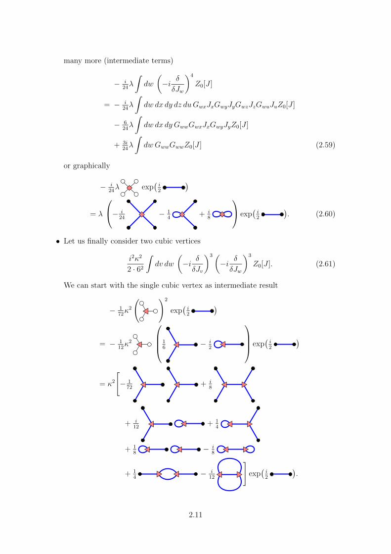
many more (intermediate terms)

− i24λ

∫dw

(−i δ

δJw

)4

Z0[J ]

= − i24λ

∫dw dx dy dz duGwxJxGwyJyGwzJzGwuJuZ0[J ]

− 624λ

∫dw dx dy GwwGwxJxGwyJyZ0[J ]

+ 3i24λ

∫dwGwwGwwZ0[J ] (2.59)

or graphically

− i24λ exp

(i2

)= λ

− i24

− 14

+ i8

exp(i2

). (2.60)

• Let us finally consider two cubic vertices

i2κ2

2 · 62

∫dv dw

(−i δδJv

)3(−i δ

δJw

)3

Z0[J ]. (2.61)

We can start with the single cubic vertex as intermediate result

− 172κ2

( )2

exp(i2

)

= − 112κ2

16

− i2

exp(i2

)

= κ2

[− 1

72+ i

8

+ i12

+ 14

+ 18

− i8

+ 14

− i12

]exp(i2

).

2.11

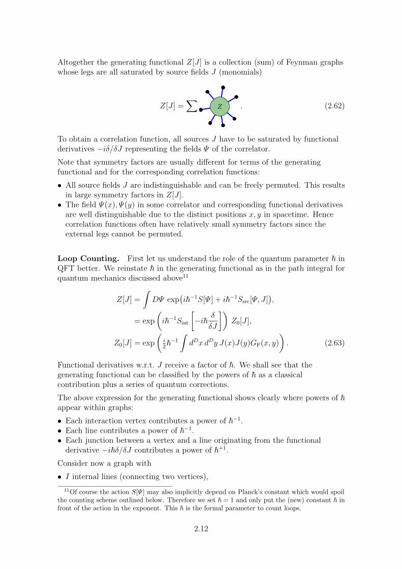
Altogether the generating functional Z[J ] is a collection (sum) of Feynman graphswhose legs are all saturated by source fields J (monomials)

Z[J ] =∑

Z . (2.62)

To obtain a correlation function, all sources J have to be saturated by functionalderivatives −iδ/δJ representing the fields Ψ of the correlator.

Note that symmetry factors are usually different for terms of the generatingfunctional and for the corresponding correlation functions:

• All source fields J are indistinguishable and can be freely permuted. This resultsin large symmetry factors in Z[J ].• The field Ψ(x), Ψ(y) in some correlator and corresponding functional derivatives

are well distinguishable due to the distinct positions x, y in spacetime. Hencecorrelation functions often have relatively small symmetry factors since theexternal legs cannot be permuted.

Loop Counting. First let us understand the role of the quantum parameter ~ inQFT better. We reinstate ~ in the generating functional as in the path integral forquantum mechanics discussed above11

Z[J ] =

∫DΨ exp

(i~−1S[Ψ ] + i~−1Ssrc[Ψ, J ]

),

= exp

(i~−1Sint

[−i~ δ

δJ

])Z0[J ],

Z0[J ] = exp

(i2~−1

∫dDx dDy J(x)J(y)GF(x, y)

). (2.63)

Functional derivatives w.r.t. J receive a factor of ~. We shall see that thegenerating functional can be classified by the powers of ~ as a classicalcontribution plus a series of quantum corrections.

The above expression for the generating functional shows clearly where powers of ~appear within graphs:

• Each interaction vertex contributes a power of ~−1.• Each line contributes a power of ~−1.• Each junction between a vertex and a line originating from the functional

derivative −i~δ/δJ contributes a power of ~+1.

Consider now a graph with

• I internal lines (connecting two vertices),

11Of course the action S[Ψ ] may also implicitly depend on Planck’s constant which would spoilthe counting scheme outlined below. Therefore we set ~ = 1 and only put the (new) constant ~ infront of the action in the exponent. This ~ is the formal parameter to count loops.

2.12

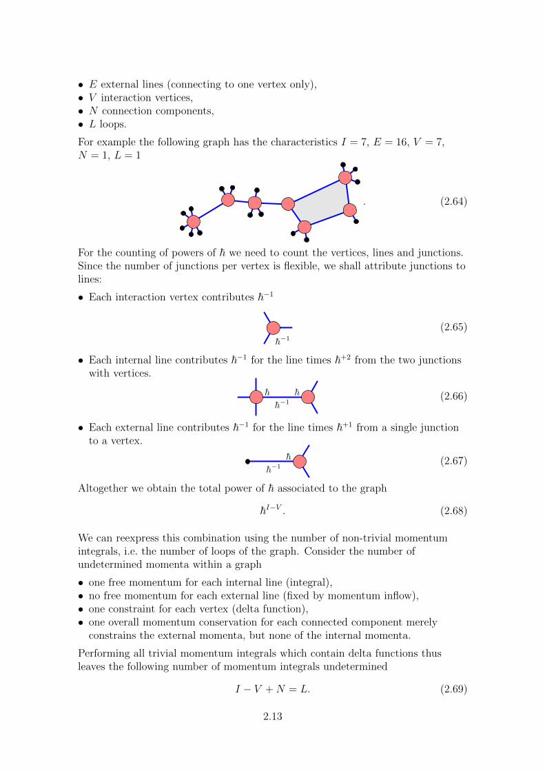
• E external lines (connecting to one vertex only),• V interaction vertices,• N connection components,• L loops.

For example the following graph has the characteristics I = 7, E = 16, V = 7,N = 1, L = 1

. (2.64)

For the counting of powers of ~ we need to count the vertices, lines and junctions.Since the number of junctions per vertex is flexible, we shall attribute junctions tolines:

• Each interaction vertex contributes ~−1

h−1(2.65)

• Each internal line contributes ~−1 for the line times ~+2 from the two junctionswith vertices.

h h

h−1(2.66)

• Each external line contributes ~−1 for the line times ~+1 from a single junctionto a vertex.

h

h−1(2.67)

Altogether we obtain the total power of ~ associated to the graph

~I−V . (2.68)

We can reexpress this combination using the number of non-trivial momentumintegrals, i.e. the number of loops of the graph. Consider the number ofundetermined momenta within a graph

• one free momentum for each internal line (integral),• no free momentum for each external line (fixed by momentum inflow),• one constraint for each vertex (delta function),• one overall momentum conservation for each connected component merely

constrains the external momenta, but none of the internal momenta.

Performing all trivial momentum integrals which contain delta functions thusleaves the following number of momentum integrals undetermined

I − V +N = L. (2.69)

2.13

This combination is the number L of non-trivial momentum integrals, i.e. thenumber of loops of the graph.

Altogether the powers of ~ now read

~I−V = ~L−N . (2.70)

This means that each momentum loop is suppressed by one power of ~. Theleading contribution at L = 0 is considered to represent classical physics. Moreoverthe number of connection components N plays a role. We shall soon return to thisresult.

2.5 Further Generating Functionals

Besides the generating functional Z[J ] there are further useful generatingfunctionals which are somewhat simpler to handle and evaluate. These summarise

• W [J ] connected graphs,• T [J ] connected tree graphs,• G[Ψ ] one-particle irreducible graphs.

Connected Graphs. The connected generating functional W [J ] is defined asthe logarithm of Z[J ] 12

W [J ] = −i~ logZ[J ], Z[J ] = exp(i~−1W [J ]). (2.71)

Just like any other generating functional, W [J ] can be represented in terms of asum over Feynman graphs. The difference w.r.t. Z[J ] is that W [J ] encodesprecisely all connected Feynman graphs. It is nice to have a formal description ofthis simpler set of graphs because it allows to reproduce all disconnected graphs.

How can this relationship be proved? It is a simple consequence of the symmetryfactors of disconnected Feynman graphs. The symmetry factor is the product of

• the symmetry factors of the connected components and• a factor of 1/n! for n equivalent connected components.

More explicitly, consider a disconnected graph Γ consisting of connected subgraphsΓk with multiplicity nk. The contribution to Z[J ] reads13

Γ [J ]

S[Γ ]=∏k

1

nk!

(Γk[J ]

S[Γk]

)nk

∈ Z[J ]. (2.72)

Here S[Γ ] denotes the symmetry factor associated to the graph Γ . The above termactually arises as one term in the multinomial and exponential

Γ

S[Γ ]∈ 1

n!

(∑k

ΓkS[Γk]

)n∈ exp

(∑k

ΓkS[Γk]

). (2.73)

12This is a pretty general relationship for generating functionals of graphs which also holds indifferent contexts.

13Here, the symbol X ∈ Y is means “X is a term of the polynomial Y ”.

2.14

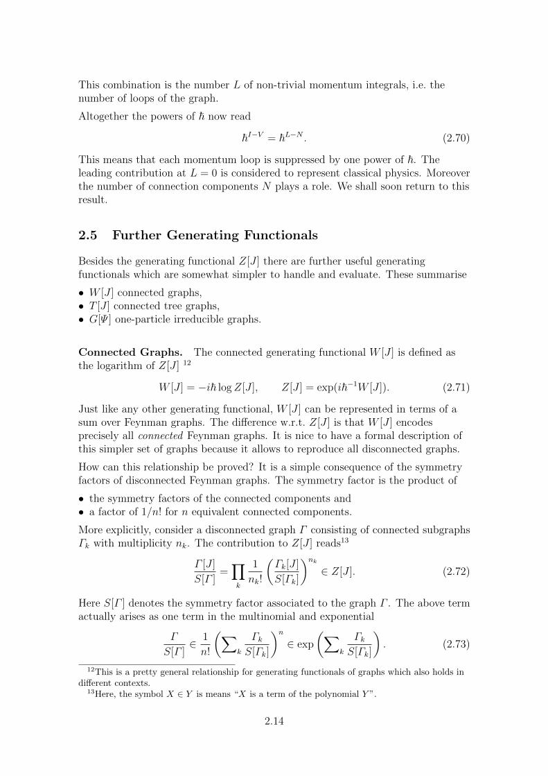
This means that exponentiating the sum of all connected graphs with appropriatesymmetry factors yields the sum of all connected and disconnected graphs withprecisely the right symmetry factors. In terms of graphs we can write Z[J ] interms of W [J ] as

Z = 1 + i W − 1

2W W − i

6W W W + . . .

= exp(i W

). (2.74)

Tree Graphs. There is a generating functional for the leading classicalcontributions. This turns out to generate precisely the tree graphs, i.e. thosewithout momentum loops.

The leading classical contributions are the most relevant contributions when ~ isvery small. The quantum constant appears as the inverse power ~−1 as a prefactorto the action in the exponent

Z[J ] =

∫DΨ exp

(i~−1S[Ψ ] + i~−1Ssrc[Ψ, J ]

). (2.75)

In the path integral this causes a strongly oscillating integrand. All contributionscancel out almost perfectly unless the exponent is stationary

δS[Ψ ]

δΨ(x)+δSsrc[Ψ, J ]

δΨ(x)=δS[Ψ ]

δΨ(x)+ J(x) = 0. (2.76)

Let us assume that there is a single stationary contribution for each source fieldconfiguration J 14 which we shall denote by Ψ = Ψ [J ]. At small ~ the path integralis dominated by this contribution (up to some irrelevant prefactor)

Z[J ] ≈ exp(i~−1T [J ]

), (2.77)

where we have introduced the functional T [J ] for the leading contribution to theexponent

T [J ] := S[Ψ [J ]] +

∫dDx J(x)Ψ [J ](x). (2.78)

What can we say about T [J ]?

First of all T [J ] is defined as the leading classical contribution to W [J ].

T [J ] = lim~→0

W [J ]. (2.79)

As such T [J ] generates a subclass of the connected graphs.

Furthermore, we have learned that the contributions to Z[J ] depend on ~ as ~L−N .For connected graphs N = 1, and therefore the graphs in W [J ] scale as ~L. Thelimit ~→ 0 then restricts to graph with L = 0, i.e. the graphs in T [J ] have no

14At least formally and perturbatively we can make this assumption.

2.15

momentum loops. Therefore T [J ] generates precisely the subclass of connectedtree graphs within Z[J ] or W [J ].

Another important observation is that T [J ] formally is the Legendretransformation of the action S[Ψ ]: The source J is defined as the functionalderivative of S[Ψ ]

J(x) = − δS[Ψ ]

δΨ(x). (2.80)

Moreover, T [J ] equals S[Ψ ] plus a term J · Ψ evaluated at the inverse Ψ = Ψ [J ] ofthe above relation.

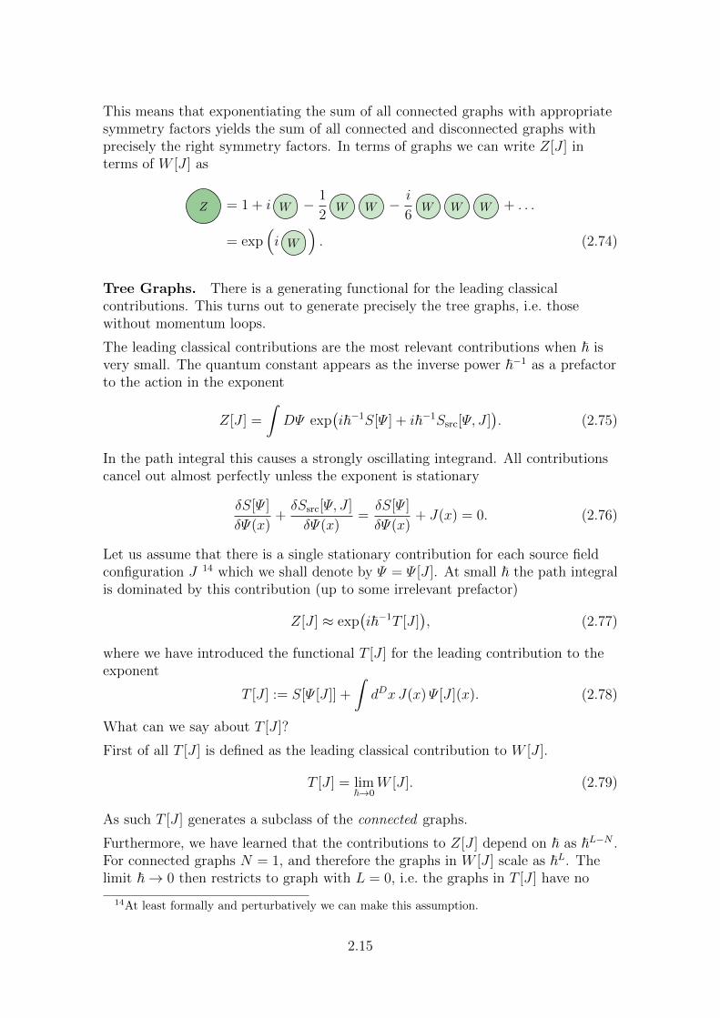
Putting the above insights together, we conclude that the Legendre transformationof some generating functional S[Ψ ] is a functional T [J ] which generates connectedtrees from the lines and vertices encoded by S0[Ψ ] and Sint[Ψ ], respectively

T [J ] = Si + 12

Si Si + 12

Si Si Si

+ 12

Si Si Si Si + 16

Si Si

Si

Si

+ . . . (2.81)

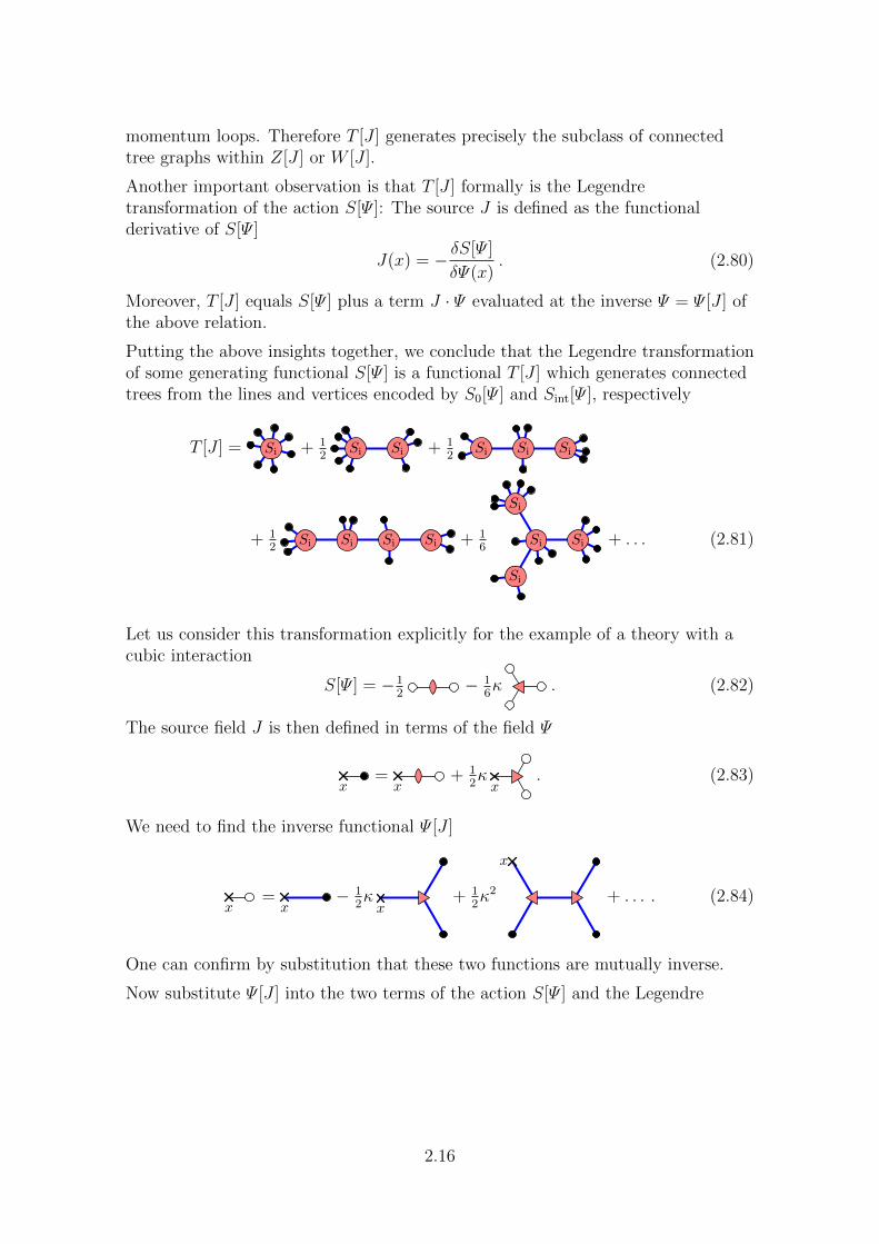
Let us consider this transformation explicitly for the example of a theory with acubic interaction

S[Ψ ] = −12

− 16κ . (2.82)

The source field J is then defined in terms of the field Ψ

x=x

+ 12κx

. (2.83)

We need to find the inverse functional Ψ [J ]

x=x

− 12κx

+ 12κ2

x

+ . . . . (2.84)

One can confirm by substitution that these two functions are mutually inverse.

Now substitute Ψ [J ] into the two terms of the action S[Ψ ] and the Legendre

2.16

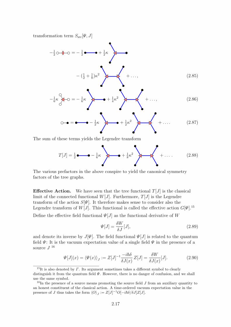
transformation term Ssrc[Ψ, J ]

−12

=− 12

+ 12κ

− (12

+ 18)κ2 + . . . , (2.85)

−16κ =− 1

6κ + 1

4κ2 + . . . , (2.86)

= − 12κ + 1

2κ2 + . . . . (2.87)

The sum of these terms yields the Legendre transform

T [J ] = 12

− 16κ + 1

8κ2 + . . . . (2.88)

The various prefactors in the above conspire to yield the canonical symmetryfactors of the tree graphs.

Effective Action. We have seen that the tree functional T [J ] is the classicallimit of the connected functional W [J ]. Furthermore, T [J ] is the Legendretransform of the action S[Ψ ]. It therefore makes sense to consider also theLegendre transform of W [J ]. This functional is called the effective action G[Ψ ].15

Define the effective field functional Ψ [J ] as the functional derivative of W

Ψ [J ] =δW

δJ[J ], (2.89)

and denote its inverse by J [Ψ ]. The field functional Ψ [J ] is related to the quantumfield Ψ : It is the vacuum expectation value of a single field Ψ in the presence of asource J 16

Ψ [J ](x) = 〈Ψ(x)〉J := Z[J ]−1 −i~δδJ(x)

Z[J ] =δW

δJ(x)[J ]. (2.90)

15It is also denoted by Γ . Its argument sometimes takes a different symbol to clearlydistinguish it from the quantum field Ψ . However, there is no danger of confusion, and we shalluse the same symbol.

16In the presence of a source means promoting the source field J from an auxiliary quantity toan honest constituent of the classical action. A time-ordered vacuum expectation value in thepresence of J thus takes the form 〈O〉J := Z[J ]−1O[−i~δ/δJ ]Z[J ].

2.17

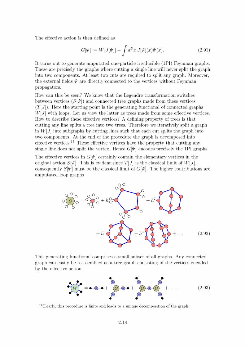
The effective action is then defined as

G[Ψ ] := W [J [Ψ ]]−∫dDx J [Ψ ](x)Ψ(x). (2.91)

It turns out to generate amputated one-particle irreducible (1PI) Feynman graphs.These are precisely the graphs where cutting a single line will never split the graphinto two components. At least two cuts are required to split any graph. Moreover,the external fields Ψ are directly connected to the vertices without Feynmanpropagators.

How can this be seen? We know that the Legendre transformation switchesbetween vertices (S[Ψ ]) and connected tree graphs made from these vertices(T [J ]). Here the starting point is the generating functional of connected graphsW [J ] with loops. Let us view the latter as trees made from some effective vertices.How to describe these effective vertices? A defining property of trees is thatcutting any line splits a tree into two trees. Therefore we iteratively split a graphin W [J ] into subgraphs by cutting lines such that each cut splits the graph intotwo components. At the end of the procedure the graph is decomposed intoeffective vertices.17 These effective vertices have the property that cutting anysingle line does not split the vertex. Hence G[Ψ ] encodes precisely the 1PI graphs.

The effective vertices in G[Ψ ] certainly contain the elementary vertices in theoriginal action S[Ψ ]. This is evident since T [J ] is the classical limit of W [J ],consequently S[Ψ ] must be the classical limit of G[Ψ ]. The higher contributions areamputated loop graphs

G = + ~ + ~2

+ ~3 + ~3 + . . . (2.92)

This generating functional comprises a small subset of all graphs. Any connectedgraph can easily be reassembled as a tree graph consisting of the vertices encodedby the effective action

W = ∗ + G ∗∗

∗+ G G∗∗

∗

∗

∗+ . . . . (2.93)

17Clearly, this procedure is finite and leads to a unique decomposition of the graph.

2.18

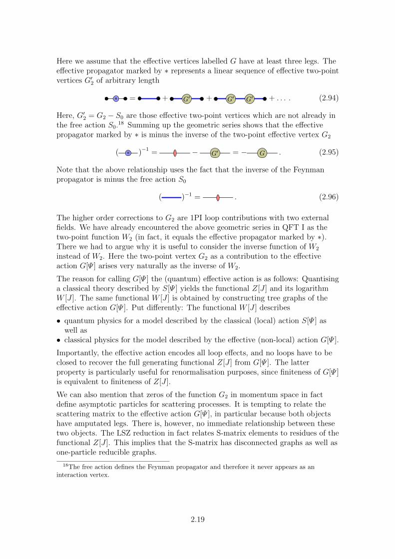
Here we assume that the effective vertices labelled G have at least three legs. Theeffective propagator marked by ∗ represents a linear sequence of effective two-pointvertices G′2 of arbitrary length

∗ = + G′ + G′ G′ + . . . . (2.94)

Here, G′2 = G2 − S0 are those effective two-point vertices which are not already inthe free action S0.18 Summing up the geometric series shows that the effectivepropagator marked by ∗ is minus the inverse of the two-point effective vertex G2

( ∗ )−1 = − G′ = − G . (2.95)

Note that the above relationship uses the fact that the inverse of the Feynmanpropagator is minus the free action S0

( )−1 = . (2.96)

The higher order corrections to G2 are 1PI loop contributions with two externalfields. We have already encountered the above geometric series in QFT I as thetwo-point function W2 (in fact, it equals the effective propagator marked by ∗).There we had to argue why it is useful to consider the inverse function of W2

instead of W2. Here the two-point vertex G2 as a contribution to the effectiveaction G[Ψ ] arises very naturally as the inverse of W2.

The reason for calling G[Ψ ] the (quantum) effective action is as follows: Quantisinga classical theory described by S[Ψ ] yields the functional Z[J ] and its logarithmW [J ]. The same functional W [J ] is obtained by constructing tree graphs of theeffective action G[Ψ ]. Put differently: The functional W [J ] describes

• quantum physics for a model described by the classical (local) action S[Ψ ] aswell as• classical physics for the model described by the effective (non-local) action G[Ψ ].

Importantly, the effective action encodes all loop effects, and no loops have to beclosed to recover the full generating functional Z[J ] from G[Ψ ]. The latterproperty is particularly useful for renormalisation purposes, since finiteness of G[Ψ ]is equivalent to finiteness of Z[J ].

We can also mention that zeros of the function G2 in momentum space in factdefine asymptotic particles for scattering processes. It is tempting to relate thescattering matrix to the effective action G[Ψ ], in particular because both objectshave amputated legs. There is, however, no immediate relationship between thesetwo objects. The LSZ reduction in fact relates S-matrix elements to residues of thefunctional Z[J ]. This implies that the S-matrix has disconnected graphs as well asone-particle reducible graphs.

18The free action defines the Feynman propagator and therefore it never appears as aninteraction vertex.

2.19

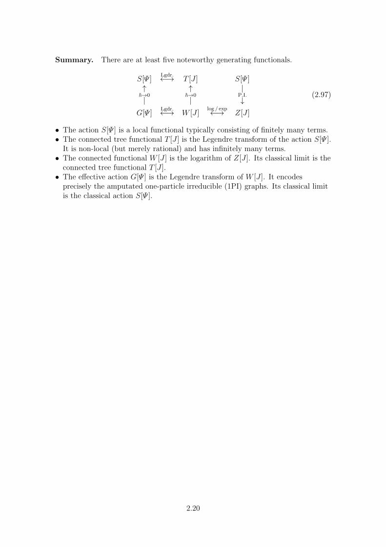
Summary. There are at least five noteworthy generating functionals.

S[Ψ ]Lgdr.←→ T [J ] S[Ψ ]

↑ ↑ |~→0 ~→0 P.I.| | ↓

G[Ψ ]Lgdr.←→ W [J ]

log / exp←→ Z[J ]

(2.97)

• The action S[Ψ ] is a local functional typically consisting of finitely many terms.• The connected tree functional T [J ] is the Legendre transform of the action S[Ψ ].

It is non-local (but merely rational) and has infinitely many terms.• The connected functional W [J ] is the logarithm of Z[J ]. Its classical limit is the

connected tree functional T [J ].• The effective action G[Ψ ] is the Legendre transform of W [J ]. It encodes

precisely the amputated one-particle irreducible (1PI) graphs. Its classical limitis the classical action S[Ψ ].

2.20

Quantum Field Theory II Chapter 3ETH Zurich, FS13 Prof. N. Beisert

16. 05. 2013

3 Lie Algebra

Symmetries are ubiquitous in physics. Mathematically they are described by theconcept of groups. They can be discrete (such as lattice symmetries in condensedmatter physics) or continuous (such as the spacetime symmetries in quantum fieldtheory). The latter are known as Lie groups. Lie groups play an important role inquantum field theory, where they serve as global spacetime and flavoursymmetries. Furthermore they prominently appear as local gauge symmetries inYang–Mills theory which is a generalisation of electrodynamics.1

3.1 Lie Groups

Yang–Mills theory is often explained in terms of N ×N unitarity matrices. Thelatter form a Lie group. Let us therefore discuss Lie groups, Lie algebras,enveloping algebras and their relationship.

Definition. A Lie group G is a group that is also a smooth manifold. The groupmultiplication G×G→ G must be a smooth map.

Example. The set of unitary matrices evidently defines a (compact) smoothmanifold, and it is a group with a smooth composition rule.

Lie groups can be distinguished by several useful properties:

• They can be simple, semi-simple or composite.• They can be real or complex (as a manifold).• They can be compact or non-compact (as a manifold).• They can be simply connected, connected or disconnected (as a manifold).• They can be finite or infinite-dimensional (as a manifold).

Composition. Simple Lie groups serve as fundamental building blocks for moregeneral Lie groups:

• A simple Lie group is a connected non-abelian Lie group which does not havenon-trivial connected normal sub-groups.2 Since only normal subgroups H of Gcan be used to define quotient spaces G/H with a group structure, simplicityessentially means that the group cannot be reduced to a smaller group.• A semi-simple Lie group is a direct product of simple Lie groups.• Composite Lie groups are direct or non-direct products of simple or abelian Lie

groups.

1As a motivation, it makes sense to get familiar with classical Yang–Mills theory at thebeginning of the next chapter before considering the more abstract topics of Lie groups in thischapter.

2A one-dimensional abelian Lie group is sometimes considered to be simple.

3.1

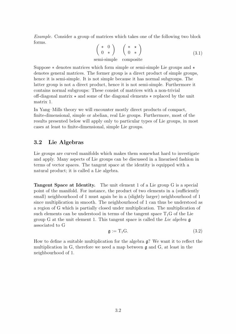
Example. Consider a group of matrices which takes one of the following two blockforms. (

∗ 00 ∗

) (∗ ?0 ∗

)semi-simple composite

(3.1)

Suppose ∗ denotes matrices which form simple or semi-simple Lie groups and ?denotes general matrices. The former group is a direct product of simple groups,hence it is semi-simple. It is not simple because it has normal subgroups. Thelatter group is not a direct product, hence it is not semi-simple. Furthermore itcontains normal subgroups: These consist of matrices with a non-trivialoff-diagonal matrix ? and some of the diagonal elements ∗ replaced by the unitmatrix 1.

In Yang–Mills theory we will encounter mostly direct products of compact,finite-dimensional, simple or abelian, real Lie groups. Furthermore, most of theresults presented below will apply only to particular types of Lie groups, in mostcases at least to finite-dimensional, simple Lie groups.

3.2 Lie Algebras

Lie groups are curved manifolds which makes them somewhat hard to investigateand apply. Many aspects of Lie groups can be discussed in a linearised fashion interms of vector spaces. The tangent space at the identity is equipped with anatural product; it is called a Lie algebra.

Tangent Space at Identity. The unit element 1 of a Lie group G is a specialpoint of the manifold. For instance, the product of two elements in a (sufficientlysmall) neighbourhood of 1 must again be in a (slightly larger) neighbourhood of 1since multiplication in smooth. The neighbourhood of 1 can thus be understood asa region of G which is partially closed under multiplication. The multiplication ofsuch elements can be understood in terms of the tangent space T1G of the Liegroup G at the unit element 1. This tangent space is called the Lie algebra gassociated to G

g := T1G. (3.2)

How to define a suitable multiplication for the algebra g? We want it to reflect themultiplication in G, therefore we need a map between g and G, at least in theneighbourhood of 1.

3.2

Exponential Map. Define a smooth map exp from a neighbourhood of 0 in g toa neighbourhood of 1 in G 3 such that4

exp(0) = 1, d exp(0) = id, exp(na) = exp(a)n. (3.3)

This map is called the exponential map. We can construct the exponential map asthe limit5

exp(a) = limn→∞

(1 +

a

n

)n. (3.4)

Here 1 + a/n is understood as an element of the Lie group in the neighbourhood of1 and raising it to some power is achieved by group multiplication. Evidently, thedefinition makes sense only for sufficiently large n, hence the limit.

Multiplication. The exponential map allows to pull back the groupmultiplication to the Lie algebra. Define a smooth map m : g× g→ g (moreprecisely on some neighbourhoods of 0 in g) such that

exp(a) exp(b) = exp(m(a, b)

). (3.5)

Now it is clear that m(a, 0) = m(0, a) = x hence

m(a, b) = a+ b+O(a)O(b). (3.6)

We see that the pull back is approximated by vector addition. Addition is anatural operation for vector spaces, and the result is evident from smoothnessproperties. This composition law is therefore not very interesting since it tellsnothing about multiplication in the underlying Lie group.

Let us therefore understand the deviation from linearity. We write explicitly theterms quadratic and of higher orders in a, b as

m(a, b) = a+ b+m2(a, b) +m≥3(a, b). (3.7)

From the above discussion we know that m2 must be bilinear. We furthermoreknow that m(a, a) = 2a. This implies that m2(a, a) = 0. Together with bilinearitywe conclude that m2 is anti-symmetric

0 = m2(a+ b, a+ b)−m2(a, a)−m2(b, b) = m2(a, b) +m2(b, a). (3.8)

3It can be extended to the whole Lie algebra g and the connected component G0 of the Liegroup G which includes the identity element 1.

4For a map f between two manifolds f : A→ B, its derivative df at a point a is a linear mapbetween the corresponding tangent spaces df(a) : TaA→ Tf(a)B. In this case the derivatived exp is defined as the identity map id on T0g = g = T1G.

5This is commonly achieved by transport via a particular vector field.

3.3

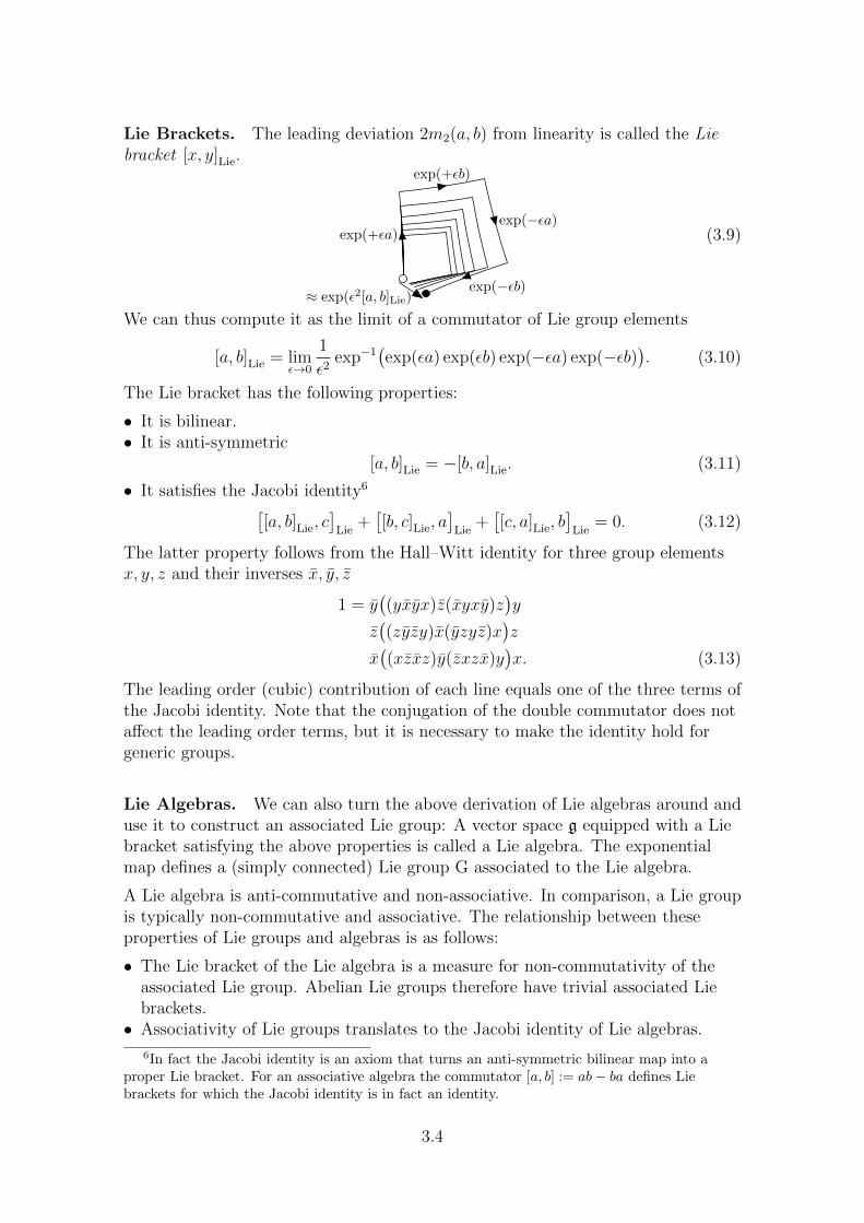
Lie Brackets. The leading deviation 2m2(a, b) from linearity is called the Liebracket [x, y]Lie.

exp(+εa)

exp(+εb)

exp(−εa)

exp(−εb)≈ exp(ε2[a, b]Lie)

(3.9)

We can thus compute it as the limit of a commutator of Lie group elements

[a, b]Lie = limε→0

1

ε2exp−1

(exp(εa) exp(εb) exp(−εa) exp(−εb)

). (3.10)

The Lie bracket has the following properties:

• It is bilinear.• It is anti-symmetric

[a, b]Lie = −[b, a]Lie. (3.11)

• It satisfies the Jacobi identity6[[a, b]Lie, c

]Lie

+[[b, c]Lie, a

]Lie

+[[c, a]Lie, b

]Lie

= 0. (3.12)

The latter property follows from the Hall–Witt identity for three group elementsx, y, z and their inverses x, y, z

1 = y((yxyx)z(xyxy)z

)y

z((zyzy)x(yzyz)x

)z

x((xzxz)y(zxzx)y

)x. (3.13)

The leading order (cubic) contribution of each line equals one of the three terms ofthe Jacobi identity. Note that the conjugation of the double commutator does notaffect the leading order terms, but it is necessary to make the identity hold forgeneric groups.

Lie Algebras. We can also turn the above derivation of Lie algebras around anduse it to construct an associated Lie group: A vector space g equipped with a Liebracket satisfying the above properties is called a Lie algebra. The exponentialmap defines a (simply connected) Lie group G associated to the Lie algebra.

A Lie algebra is anti-commutative and non-associative. In comparison, a Lie groupis typically non-commutative and associative. The relationship between theseproperties of Lie groups and algebras is as follows:

• The Lie bracket of the Lie algebra is a measure for non-commutativity of theassociated Lie group. Abelian Lie groups therefore have trivial associated Liebrackets.• Associativity of Lie groups translates to the Jacobi identity of Lie algebras.

6In fact the Jacobi identity is an axiom that turns an anti-symmetric bilinear map into aproper Lie bracket. For an associative algebra the commutator [a, b] := ab− ba defines Liebrackets for which the Jacobi identity is in fact an identity.

3.4

3.3 Enveloping Algebras

In quantum physics, we are not only interested in Lie algebra elements and theirLie brackets, but we would also like to be able to take associative products of them.

Definition. There is a useful concept to embed a Lie algebra into a (much)bigger associative algebra with unit element. This is the (universal) envelopingalgebra U(g) of a Lie algebra g. Its elements are ordered polynomials of theelements of the Lie algebra g. For example, if a, b, c ∈ g then the monomialsabc, acb, baac, . . ., as well as their linear combinations, are elements of U(g). Theproduct of two monomials X, Y is defined by their concatenation,

X · Y = XY (3.14)

Moreover, the Lie brackets are encoded in the enveloping algebra by identifyingthem with commutators, i.e. for all a, b ∈ g

[a, b]Lie ≡ [a, b] = ab− ba. (3.15)

To make this identification compatible with products we must also demand thefollowing: If [a, b]Lie = c then for any X, Y ∈ U(g)

XabY −XbaY ≡ XcY. (3.16)

Therefore the enveloping algebra can be defined as the space

U(g) =∞⊕n=0

g⊗n/ (

[·, ·] ≡ [·, ·]Lie

). (3.17)

Since the identification of commutators effectively removes all asymmetries withinmonomials (by shifting them to shorter monomials), we can also write the vectorspace of the enveloping algebra as a symmetric tensor product

U(g) '∞⊕n=0

gn. (3.18)

Properties. The enveloping algebra U(g) clearly includes the Lie algebra g asthe linear polynomials. Furthermore, it (more precisely its completion) alsoincludes the associated Lie group G since the exponential map acts within U(g)

exp(X) = limn→∞

(1 +

X

n

)n=∞∑n=0

1

n!Xn. (3.19)

In that sense the enveloping algebra U(g) contains a Lie algebra g, the associatedLie group G as well as many other elements which belong to neither of the two.7

7In physics these three terms are sometimes confused. In those cases it is safe to assume theenveloping algebra.

3.5

3.4 Representations

Let us now introduce some basic elements of Lie theory, in particular those whichwill be relevant to Yang–Mills theory. Fields have particular transformationproperties under gauge transformations. Mathematically, their transformationrules are described by representations.

Definition. A representation R of a Lie group G is a map from the group toendomorphisms of some vector space V (operators, linear maps or matrices actingon the space)

R : G→ End(V). (3.20)

The representation must reflect the composition law of G by operator composition(matrix multiplication), i.e. for all h, k, l ∈ G

hk = l =⇒ R(h)R(k) = R(l). (3.21)

The operator R(h) is called a representation of the element h.

The definition of a representation R of a Lie algebra g is analogous. It is a linearmap from the algebra to endomorphisms of some space V

R : g→ End(V). (3.22)

The representation must reflect the Lie bracket of g as a commutator[A,B] := AB −BA of operators, i.e. for all a, b, c ∈ g

[a, b]Lie = c =⇒ [R(a), R(b)] = R(c). (3.23)

The representation of Lie brackets in terms of commutators is compatible withtheir properties: The commutator is evidently bilinear, anti-symmetric, and itobeys the Jacobi identity.

Finally, the enveloping algebra U(g) has representations as well

R : U(g)→ End(V). (3.24)

They must obey the multiplication rule for all X, Y, Z ∈ U(g)

XY = Z =⇒ R(X)R(Y ) = R(Z). (3.25)

This rule is the same as for Lie groups, hence we will not specify this caseexplicitly in what follows.

By focusing on the unit element, it is clear that every representation of G has anassociated representation of g. The converse does not exactly hold due to potentialglobal issues of the group G.8 For example, only a discrete subset of therepresentation of g = u(1) = R lift to representations of G = U(1) = S1 becausethe latter must respect the fact that rotations by 2π are trivial. Finally,representations of g trivially lift to U(g).

8It should hold when G is simply connected.

3.6

The space V is called a representation space or a module of the group, algebra orenveloping algebra (in physics it is sometimes also sloppily called a representation).The dimension DR of the representation R is defined as the dimension of V

DR = dimR := dimV. (3.26)

Adjoint and Trivial Representations. A distinguished representation of anyLie algebra g is the adjoint representation on the Lie algebra itself

ad : g→ End(g), ad(a)b = [a, b]Lie. (3.27)

The Jacobi identity ensures that ad is a proper representation since it guaranteesthat for any a, b ∈ g

ad([a, b]Lie

)= [ad(a), ad(b)]. (3.28)

This becomes clear once applied to some c ∈ g and using anti-symmetry of the Liebrackets

ad([a, b]Lie)c =[[a, b]Lie, c

]Lie,

− ad(a) ad(b)c = −[a, [b, c]Lie

]Lie

=[[b, c]Lie, a

]Lie,

+ ad(b) ad(a)c = +[b, [a, c]Lie

]Lie

=[[c, a]Lie, b

]Lie. (3.29)

The vector fields always transform in the adjoint representation of the gauge group.

The adjoint representation for the Lie group (and equivalently for the envelopingalgebra) reads9

Ad : G→ End(g), Ad(h)b = hbh−1. (3.30)

Another representation which exists in any Lie algebra is the trivial one (typicallydefined on a one-dimensional space V). For a ∈ g and h ∈ G

triv(a) = 0, triv(h) = id . (3.31)

Finally, there always exists a representation on the enveloping algebra since itnaturally contains the Lie algebra and group

env : g,G→ End(U(g)), env(h)X = hX. env(a)X = aX, (3.32)

This representation is useful for formal reasons, since in some sense it is maximaland contains all other representations.

Sums and Tensor Products. Representations can be combined to form biggerrepresentations. There are two main operations: direct sums and tensor products.In Yang–Mills theory these operations correspond to collections and products offields.

9Here the product b′ = hbh−1 of group and algebra elements can be understood in terms ofthe group product h(1 + εb)h−1 = (1 + εb′) with the middle factor in the neighbourhood of 1.

3.7

Suppose R1, R2 are two representations of a Lie group, Lie algebra or anenveloping algebra on the spaces V1,V2. The direct sum R1⊕2 of tworepresentations R1, R2 on the space V1⊕2 = V1 ⊕ V2 is defined as the blockdiagonal matrix acting on the space (V1,V2)

R1⊕2 =

(R1 00 R2

). (3.33)

Tensor product representations R1⊗2 of an element of the group (or envelopingalgebra) on the space V1⊗2 = V1 ⊗ V2 are defined as

R1⊗2(h) = R1(h)⊗R2(h), (3.34)

The definition for a Lie algebra element is slightly different

R1⊗2(a) = R1(a)⊗ id + id⊗R2(a). (3.35)

Evidently, all three definitions of R satisfy the axioms of representations providedthat R1, R2 are proper representations.

Tensor products of two or more identical representations R are special since theirtensor product naturally decomposes into certain symmetric components. Forexample, for the tensor product V⊗ V of two identical spaces V we can define apermutation operator P ∈ End(V⊗ V)

P (v1 ⊗ v2) := v2 ⊗ v1. (3.36)

It can be used to construct two projectors P± onto the symmetric andanti-symmetric subspaces V± of V⊗ V

P± = 12(id± P ), (3.37)

where id is the identity acting on V⊗V. Now the definitions of the tensor productrepresentation R⊗R commute with the permutation operator P , and hence alsowith the projectors P±. Therefore it will act as a direct sum of representation R±

on the subspaces V±

R⊗R = R+ ⊕R−, R± = P±(R⊗R)P±. (3.38)

For more than two identical representations, tensor products will split into severalcomponents with particular permutation symmetries determined byrepresentations of the discrete permutation group.10

Properties. The structure of a representation can have various properties:

• It can be reducible or irreducible (simple). An irreducible representation has noproper sub-representation. It is also called irrep for short.

10A useful tool in this respect are Young tableaux/diagrams, see below.

3.8

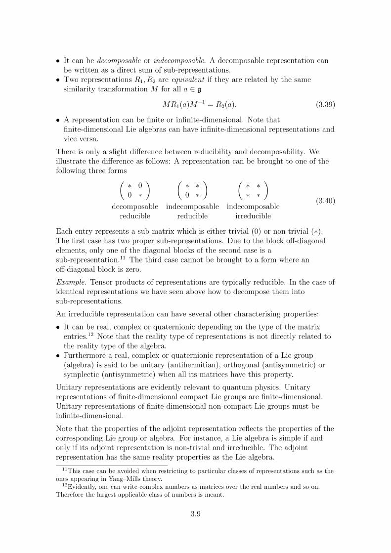
• It can be decomposable or indecomposable. A decomposable representation canbe written as a direct sum of sub-representations.• Two representations R1, R2 are equivalent if they are related by the same

similarity transformation M for all a ∈ g

MR1(a)M−1 = R2(a). (3.39)

• A representation can be finite or infinite-dimensional. Note thatfinite-dimensional Lie algebras can have infinite-dimensional representations andvice versa.

There is only a slight difference between reducibility and decomposability. Weillustrate the difference as follows: A representation can be brought to one of thefollowing three forms(

∗ 00 ∗

) (∗ ∗0 ∗

) (∗ ∗∗ ∗

)decomposable indecomposable indecomposable

reducible reducible irreducible

(3.40)

Each entry represents a sub-matrix which is either trivial (0) or non-trivial (∗).The first case has two proper sub-representations. Due to the block off-diagonalelements, only one of the diagonal blocks of the second case is asub-representation.11 The third case cannot be brought to a form where anoff-diagonal block is zero.

Example. Tensor products of representations are typically reducible. In the case ofidentical representations we have seen above how to decompose them intosub-representations.

An irreducible representation can have several other characterising properties:

• It can be real, complex or quaternionic depending on the type of the matrixentries.12 Note that the reality type of representations is not directly related tothe reality type of the algebra.• Furthermore a real, complex or quaternionic representation of a Lie group

(algebra) is said to be unitary (antihermitian), orthogonal (antisymmetric) orsymplectic (antisymmetric) when all its matrices have this property.

Unitary representations are evidently relevant to quantum physics. Unitaryrepresentations of finite-dimensional compact Lie groups are finite-dimensional.Unitary representations of finite-dimensional non-compact Lie groups must beinfinite-dimensional.

Note that the properties of the adjoint representation reflects the properties of thecorresponding Lie group or algebra. For instance, a Lie algebra is simple if andonly if its adjoint representation is non-trivial and irreducible. The adjointrepresentation has the same reality properties as the Lie algebra.

11This case can be avoided when restricting to particular classes of representations such as theones appearing in Yang–Mills theory.

12Evidently, one can write complex numbers as matrices over the real numbers and so on.Therefore the largest applicable class of numbers is meant.

3.9

3.5 Invariants

Lie algebras have several invariant objects which serve various important purposes.For instance the quadratic form provides a natural metric for the Lie algebramanifold. Consequently, it can be used to translate between vectors and covectors.In the Yang–Mills theory, they are not only important for defining Feynmanpropagators, but also relevant for consistency issues such as anomalies of gaugesymmetry.

Invariant Elements. Consider a simple (finite-dimensional) Lie algebra g. Upto rescaling it has a unique invariant symmetric bilinear form K ∈ (g∗)2, knownas the Killing form. Symmetry and invariance means that for all a, b, c ∈ g

K(a, b) = K(b, a), K([c, a]Lie, b) +K(a, [c, b]Lie) = 0. (3.41)

This form can be constructed easily using some representation R, for exampleusing the adjoint representations R = ad

TrR(a)R(b) ∼ K(a, b). (3.42)

The Killing form of a semi-simple Lie algebra is invertible. Therefore there is acorresponding invariant element C2 ∈ g2 called the Casimir invariant. Thought ofas a matrix, it is the inverse of the Killing form K. It obeys the invarianceproperty for all a ∈ g (

ad(a)⊗ id + id⊗ ad(a))C2 = 0. (3.43)

The quadratic invariant can also be viewed as a quadratic element of theenveloping algebra U(g). The invariance property implies that it is in the centre ofU(g), i.e. it commutes with all X ∈ U(g)

C2X = XC2. (3.44)

Therefore an irreducible representation of C2 is necessarily proportional to theidentity operator

R(C2) ∼ idR . (3.45)

For example, for g = su(2) the Casimir invariant C2 is the total spin operator.

For most Lie algebras, there are analogous invariant polynomials Cn ∈ gn ofhigher degree n. Which ones of these higher invariant exists depends on the Liealgebra. The quadratic invariant exists for every simple Lie algebra.

There is a curious relationship between the invariants of g and the topology of theassociated (connected, universal covering) Lie group G: In terms of cohomology,the group manifold is equivalent to a product of odd-dimensional spheres

G '∏k

S2nk−1. (3.46)

For every independent invariant of degree nk there is a sphere of dimension2nk − 1.13

13This well-known result of Lie groups is again not immediately relevant for our course.

3.10

Structure Constants. For non-abelian gauge theories it is convenient to choosesome basis Ta for a Lie algebra g. The elements Ta are called generators of g. Inquantum physics, the basis is typically chosen to be imaginary

a = iaaTa. (3.47)

One the one hand, this choice usually makes the representation of Ta hermitianwhich is convenient because it guarantees real eigenvalues. On the other hand, itintroduces several unnecessary factors of i. For instance, a group element h istypically parametrised via the exponential map as

h = exp(iaaTa). (3.48)

Now that we have a basis, we can expand the Lie brackets in terms of the structureconstants fab

c

[Ta, Tb]Lie = ifabcTc. (3.49)

For a real algebra, the structure constants fabc must be real.

Furthermore we expand the invariant bilinear form in this basis as

K(Ta, Tb) = kab. (3.50)

For a real, compact, simple Lie algebra, the matrix kab is positive-definite. By asuitable choice of (orthonormal) basis Ta we can adjust kab to be the unit matrix

kab = δab. (3.51)

It is convenient to make this assumption, but for the time being we shall keep thenotation kab and introduce its inverse kab.

For semi-simple Lie algebras the matrix kab is non-degenerate. It can be used toraise and lower indices. For instance we can uniformise the indices of the structureconstants

fabc = fabdkdc. (3.52)

These structure constants are totally anti-symmetric in all three indices

fabc = −fbac = −facb. (3.53)

Antisymmetry of the former two indices follows by definition. Antisymmetry of thelatter indices follows from invariance of K

0 = K([Tc, Ta]Lie, Tb) +K(Ta, [Tc, Tb]Lie) = ifcab + ifcba (3.54)

Now we can also consider a representation TRa of the basis Ta, namely

TRa = R(Ta). (3.55)

Evidently the matrices TRa obey the commutator identity

[TRa , TRb ] = ifab

cTRc . (3.56)

A special case is the adjoint representation

(T ada )Tb = [Ta, Tb]Lie = ifab

cTc. (3.57)

Therefore, the adjoint representation T ada is a matrix whose elements are the

structure constants(T ad

a )bc = ifab

c. (3.58)

3.11

Constants for Representations. We have seen above that the invariantelements obey identities for representations which hold up certain factors ofproportionality. These factors can be used to characterise representations. Theyalso appear as characteristic quantities in computations of Feynman diagrams. Letus therefore discuss them in more detail.

For an irreducible representation R we know that the trace of two representationmatrices yields the Killing form

TrTRa TRb = BRkab. (3.59)

The factor of proportionality BR depends on the particular representation R. Italso depends on the normalisation as we shall discuss later. For the adjointrepresentation we can write this relation in terms of structure constants

− facdfbdc = Badkab. (3.60)

An irreducible representation of the quadratic Casimir invariantC2 := kabTaTb ∈ U(g) now takes the form

R(C2) = kabTRa TRb = CR

2 idR . (3.61)

The eigenvalue CR2 is a characteristic quantity of the irreducible representation R.

For example, the constant Cj2 for a spin-j representation of su(2) evidently is

proportional to j(j + 1).

By taking the trace of the above identity we can establish a relationship betweenthe constants BR and CR

2

CR2 Tr idR = kab TrTRa T

Rb = BRkabkab. (3.62)

Now Tr idR = DR is the dimension of the representation R. Furthermorekabkab = Tr idad = Dad = dim g is the dimension of the algebra. We thus have therelation

DadBR = DRCR2 . (3.63)

Therefore all the constants BR can be determined in terms of the constants CR2 . In

particular, for the adjoint representation it implies the equality of the twoconstants

Bad = Cad2 . (3.64)

This can also be seen directly

Cad2 δec = (kabT ad

a T adb )c

f = −kabfacdfbde = Badkcfkfe. (3.65)

Also the higher invariants Cn have characterising eigenvalues CRn on irreducible

representations RR(Cn) = CR

n id . (3.66)

Note that there is some arbitrariness in the definition of the above constants BR

and CRn . We can simultaneously rescale all generators Ta and the structure

constants fabc by a common factor of α

(T ′)a = αTa, (f ′)abc = αfab

c. (3.67)

3.12

This transformation does not change any of the above relations. However, theconstants related to the invariants must rescale with a factor of α2

(B′)R = α2BR, (C ′2)R = α2CR2 . (3.68)

This result shows that there is no universal definition for the BR and CR2 .

However, fixing one of them, fixes all the others.

Moreover, we are in principle free to rescale the definition of the structureconstants [Ta, Tb]Lie ∼ fab

cTc and of the invariants kab, B and Cn. This would addfurther arbitrariness to their definitions.

3.6 Unitary and Other Algebras

Finite-dimensional simple Lie algebras have been classified. Let us review theclassification and then discuss the unitary algebras is more detail.

Classification. Finite-dimensional, complex, simple Lie groups have beenclassified: There are four infinite families an, bn, cn and dn. They are related to thethree main classes of matrix algebras

type matrix algebra symbol matrix group namean sl(n+ 1) special linearbn so(2n+ 1) orthogonal (odd)cn sp(2n) symplecticdn so(2n) orthogonal (even)

(3.69)

Here, the index of the algebras denotes their rank, a characteristic number forsimple Lie algebras.

The matrix algebras have particular properties which are stable under takingcommutators

• The commutator of two N ×N matrices is traceless. Hence, traceless matricesform the special linear Lie algebra sl(N)

A ∈ sl(N) : TrA = 0. (3.70)

• Anti-symmetric N ×N matrices w.r.t. an invertible symmetric metric M (e.g.M = 1) close under taking commutators. Therefore they form the orthogonalLie algebra so(N)

A ∈ so(N) : AT = −MAM−1, MT = M. (3.71)

• Anti-symmetric N ×N matrices with respect to an invertible anti-symmetricmetric E close under taking commutators. They form the symplectic Lie algebrasp(N)

A ∈ sp(N) : AT = −EAE−1, ET = −E. (3.72)

3.13

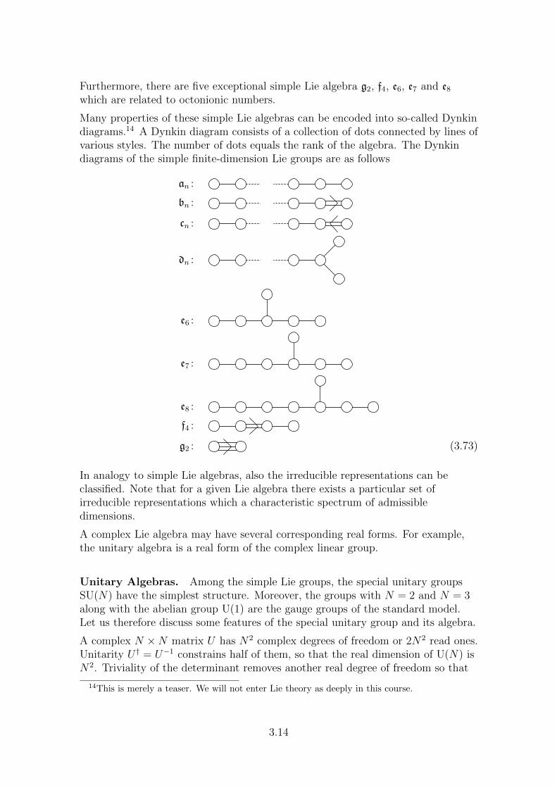
Furthermore, there are five exceptional simple Lie algebra g2, f4, e6, e7 and e8

which are related to octonionic numbers.

Many properties of these simple Lie algebras can be encoded into so-called Dynkindiagrams.14 A Dynkin diagram consists of a collection of dots connected by lines ofvarious styles. The number of dots equals the rank of the algebra. The Dynkindiagrams of the simple finite-dimension Lie groups are as follows

an :

bn :

cn :

dn :

e6 :

e7 :

e8 :

f4 :

g2 : (3.73)

In analogy to simple Lie algebras, also the irreducible representations can beclassified. Note that for a given Lie algebra there exists a particular set ofirreducible representations which a characteristic spectrum of admissibledimensions.

A complex Lie algebra may have several corresponding real forms. For example,the unitary algebra is a real form of the complex linear group.

Unitary Algebras. Among the simple Lie groups, the special unitary groupsSU(N) have the simplest structure. Moreover, the groups with N = 2 and N = 3along with the abelian group U(1) are the gauge groups of the standard model.Let us therefore discuss some features of the special unitary group and its algebra.

A complex N ×N matrix U has N2 complex degrees of freedom or 2N2 read ones.Unitarity U † = U−1 constrains half of them, so that the real dimension of U(N) isN2. Triviality of the determinant removes another real degree of freedom so that

14This is merely a teaser. We will not enter Lie theory as deeply in this course.

3.14

the dimension of SU(N) is N2 − 1.

Dad = N2 − 1. (3.74)

The corresponding Lie algebra su(N) is the commutator algebra of tracelessanti-hermitian matrices A. Correspondingly, they have N2 − 1 real degrees offreedom.

Since the Lie group and algebra are both formulated in terms of matrices, we knowthat

G, g ⊂ End(CN). (3.75)

Therefore it is straight-forward to construct an N -dimensional representation, theso-called defining or fundamental representation (with v ∈ CN)

def(A)v = Av, def(U)v = Uv, Ddef = N. (3.76)

There is in fact another N -dimensional representation, the conjugate definingrepresentation

def(A)v = A∗v = −ATv, def(U)v = U∗v, Ddef = N. (3.77)

The adjoint representation is a representation on the (N2 − 1)-dimensional space g15

ad(A)B = [A,B], Ad(U)B = UBU−1. (3.78)

So we know that the unitary algebras have at least four (irreducible)representations: trivial, adjoint, defining and conjugate defining. Tensor productsof these lead to infinitely many more irreducible representations.

Tensor Product Representations. Let us consider tensor products of thedefining representations.

We have already seen that tensor products of identical representations aredecomposable into various symmetric components. The tensor product of twooriginal defining representations can thus be written as

def ⊗ def = sym⊕ alt. (3.79)

Here sym and alt denote the symmetric and anti-symmetric or alternatingcomponents of the full tensor product. For the unitary algebras theserepresentations turn out to be irreducible.

The same applies to the tensor product of two conjugate defining representations,

def ⊗ def = sym⊕ alt. (3.80)

15It is sometime tempting to confuse the defining with the adjoint representation since bothcan be formulated simply in terms of the N ×N matrix A. The distinction becomes clearer whenviewing the representation space g as a (N2 − 1)-dimensional vector space rather than a subspaceof matrices.

3.15

Here sym and alt denote the conjugate representations of sym and alt, respectively.

The tensor product of mixed defining representations turns out to decompose intoirreps as well

def ⊗ def = ad⊕ triv. (3.81)

This decomposition does not follow from general arguments such as the tensorproducts of identical representations. It is a characteristic feature of the unitaryalgebras su(N).

Finite-dimensional irreps of the unitary algebras su(N) have been classified andtheir tensor products are well understood. A useful tool in this regard are Youngdiagrams (or tableaux) and Dynkin labels.16

Young diagrams are heaps of boxes. They describe certain symmetrisation classesor equivalently representations of the symmetric group. A single box correspondsto the defining representation. The conjugate fundamental representationcorresponds to a vertical stack of N − 1 boxes. The adjoint representation adds asingle box to the right of the topmost box. The trivial representation has no boxwritten as a dot. For example, for N = 5

def = , def = , ad = , triv = •. (3.82)

Horizontal stacks of boxes correspond to symmetrisation; vertical stackscorrespond to anti-symmetrisation. For example, the above decomposition of thetensor products of two defining representations can be expressed as follows

⊗ = ⊕ ,

⊗ = ⊕ ,

⊗ = ⊕ •. (3.83)

Young tableaux are useful tools to work with representations of su(N). Forinstance, there are rules for computing the dimension of irreps and rules for thedecomposition of tensor products.

Dynkin labels are a rewriting of the shape of Young tableaux in terms of a set ofinteger numbers, e.g. for N = 5

def = [1000], def = [0001], ad = [1001]. (3.84)

Each of these numbers is associated to one of the dots of the Dynkin diagram forthe Lie algebra.

[abcd] ≡a b c d

. (3.85)

Therefore the classification in terms of Dynkin labels applies to all simple Liealgebras, and not just to su(N).

16This topic is far beyond the scope of this course, but a very nice topic of group theory andcombinatorics, so let us give a flavour.

3.16

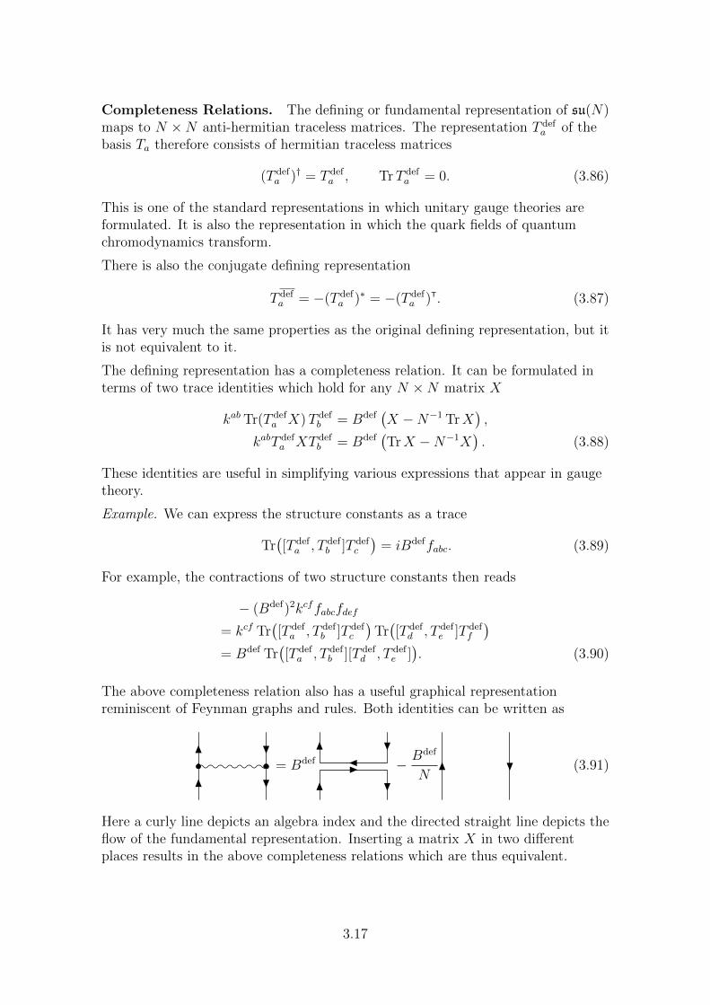
Completeness Relations. The defining or fundamental representation of su(N)maps to N ×N anti-hermitian traceless matrices. The representation T def

a of thebasis Ta therefore consists of hermitian traceless matrices

(T defa )† = T def

a , TrT defa = 0. (3.86)

This is one of the standard representations in which unitary gauge theories areformulated. It is also the representation in which the quark fields of quantumchromodynamics transform.

There is also the conjugate defining representation

T defa = −(T def

a )∗ = −(T defa )T. (3.87)

It has very much the same properties as the original defining representation, but itis not equivalent to it.

The defining representation has a completeness relation. It can be formulated interms of two trace identities which hold for any N ×N matrix X

kab Tr(T defa X)T def

b = Bdef(X −N−1 TrX

),

kabT defa XT def

b = Bdef(TrX −N−1X

). (3.88)

These identities are useful in simplifying various expressions that appear in gaugetheory.

Example. We can express the structure constants as a trace

Tr([T defa , T def

b ]T defc

)= iBdeffabc. (3.89)

For example, the contractions of two structure constants then reads

− (Bdef)2kcffabcfdef

= kcf Tr([T defa , T def

b ]T defc

)Tr([T defd , T def

e ]T deff

)= Bdef Tr

([T defa , T def

b ][T defd , T def

e ]). (3.90)

The above completeness relation also has a useful graphical representationreminiscent of Feynman graphs and rules. Both identities can be written as

= Bdef − Bdef

N(3.91)

Here a curly line depicts an algebra index and the directed straight line depicts theflow of the fundamental representation. Inserting a matrix X in two differentplaces results in the above completeness relations which are thus equivalent.

3.17

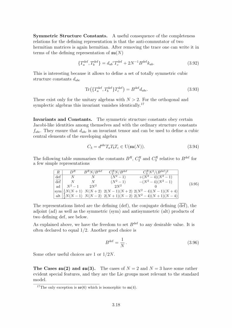
Symmetric Structure Constants. A useful consequence of the completenessrelations for the defining representation is that the anti-commutator of twohermitian matrices is again hermitian. After removing the trace one can write it interms of the defining representation of su(N)

T defa , T def

b = dabcT defc + 2N−1Bdefkab. (3.92)

This is interesting because it allows to define a set of totally symmetric cubicstructure constants dabc

Tr(T def

a , T defb T def

c

)= Bdefdabc. (3.93)

These exist only for the unitary algebras with N > 2. For the orthogonal andsymplectic algebras this invariant vanishes identically.17

Invariants and Constants. The symmetric structure constants obey certainJacobi-like identities among themselves and with the ordinary structure constantsfabc. They ensure that dabc is an invariant tensor and can be used to define a cubiccentral elements of the enveloping algebra

C3 = dabcTaTbTc ∈ U(su(N)). (3.94)

The following table summarises the constants BR, CR2 and CR

3 relative to Bdef fora few simple representations

R DR BRN/Bdef CR2 N/Bdef CR3 N

2/(Bdef)2

def N N (N2 − 1) +(N2 − 4)(N2 − 1)

def N N (N2 − 1) −(N2 − 4)(N2 − 1)ad N2 − 1 2N2 2N2 0

sym 12N(N + 1) N(N + 2) 2(N − 1)(N + 2) 2(N2 − 4)(N − 1)(N + 4)

alt 12N(N − 1) N(N − 2) 2(N + 1)(N − 2) 2(N2 − 4)(N + 1)(N − 4)

(3.95)

The representations listed are the defining (def), the conjugate defining (def), theadjoint (ad) as well as the symmetric (sym) and antisymmetric (alt) products oftwo defining def, see below.

As explained above, we have the freedom to set Bdef to any desirable value. It isoften declared to equal 1/2. Another good choice is

Bdef =1

N. (3.96)

Some other useful choices are 1 or 1/2N .

The Cases su(2) and su(3). The cases of N = 2 and N = 3 have some ratherevident special features, and they are the Lie groups most relevant to the standardmodel.

17The only exception is so(6) which is isomorphic to su(4).

3.18

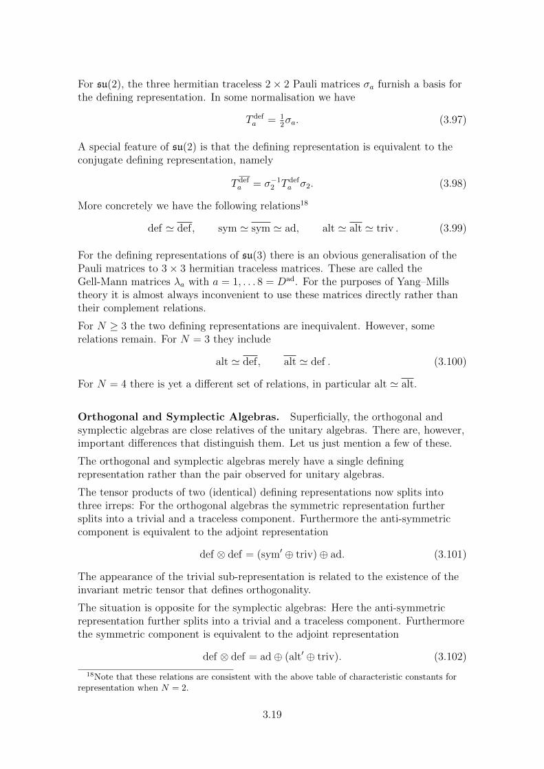
For su(2), the three hermitian traceless 2× 2 Pauli matrices σa furnish a basis forthe defining representation. In some normalisation we have

T defa = 1

2σa. (3.97)

A special feature of su(2) is that the defining representation is equivalent to theconjugate defining representation, namely

T defa = σ−1

2 T defa σ2. (3.98)

More concretely we have the following relations18

def ' def, sym ' sym ' ad, alt ' alt ' triv . (3.99)

For the defining representations of su(3) there is an obvious generalisation of thePauli matrices to 3× 3 hermitian traceless matrices. These are called theGell-Mann matrices λa with a = 1, . . . 8 = Dad. For the purposes of Yang–Millstheory it is almost always inconvenient to use these matrices directly rather thantheir complement relations.

For N ≥ 3 the two defining representations are inequivalent. However, somerelations remain. For N = 3 they include

alt ' def, alt ' def . (3.100)

For N = 4 there is yet a different set of relations, in particular alt ' alt.

Orthogonal and Symplectic Algebras. Superficially, the orthogonal andsymplectic algebras are close relatives of the unitary algebras. There are, however,important differences that distinguish them. Let us just mention a few of these.

The orthogonal and symplectic algebras merely have a single definingrepresentation rather than the pair observed for unitary algebras.

The tensor products of two (identical) defining representations now splits intothree irreps: For the orthogonal algebras the symmetric representation furthersplits into a trivial and a traceless component. Furthermore the anti-symmetriccomponent is equivalent to the adjoint representation

def ⊗ def = (sym′ ⊕ triv)⊕ ad. (3.101)

The appearance of the trivial sub-representation is related to the existence of theinvariant metric tensor that defines orthogonality.

The situation is opposite for the symplectic algebras: Here the anti-symmetricrepresentation further splits into a trivial and a traceless component. Furthermorethe symmetric component is equivalent to the adjoint representation

def ⊗ def = ad⊕ (alt′ ⊕ triv). (3.102)

18Note that these relations are consistent with the above table of characteristic constants forrepresentation when N = 2.

3.19

The appearance of the trivial sub-representation is related to the existence of theinvariant tensor that defines the symplectic structure.

Most of the properties, relations and tools of unitary algebras generalise in someway to the orthogonal and symplectic algebras. Usually they will be somewhatmore elaborate than their basic unitary counterparts.

3.20

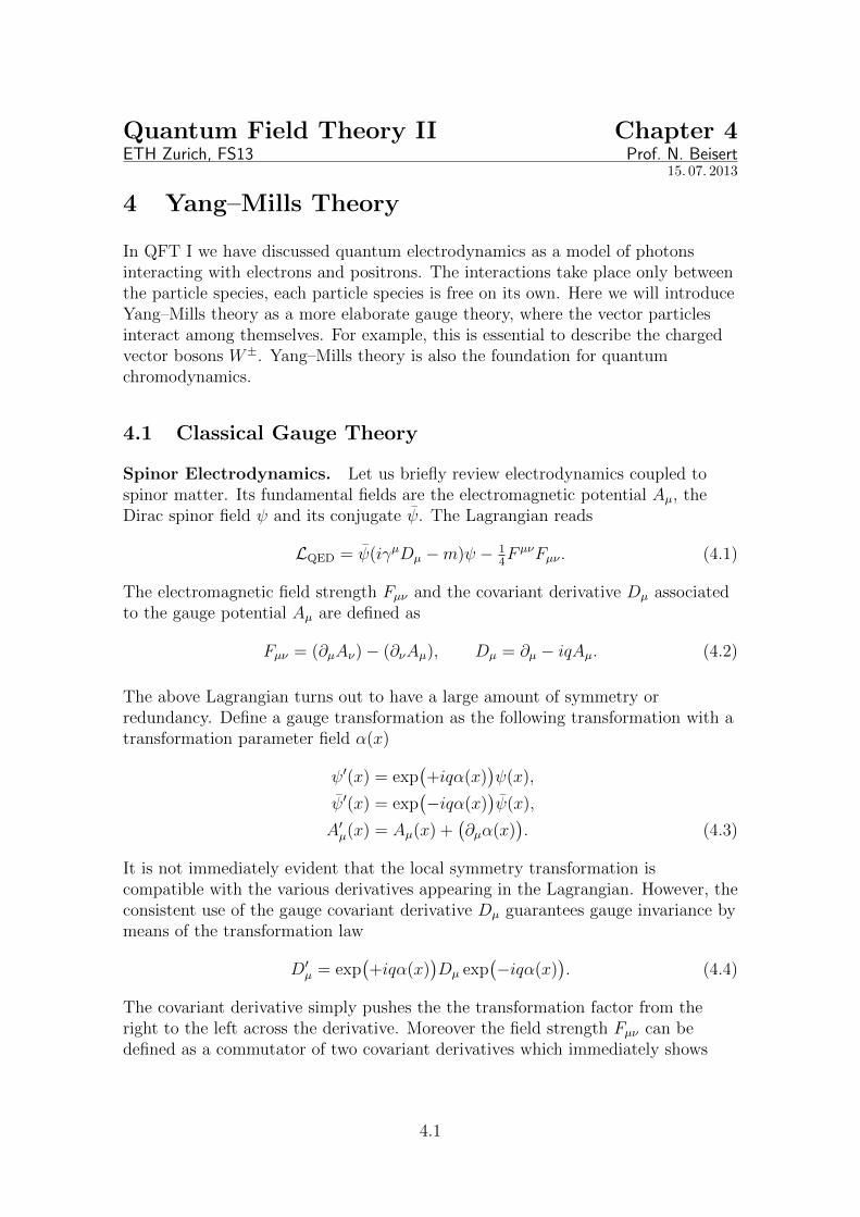
Quantum Field Theory II Chapter 4ETH Zurich, FS13 Prof. N. Beisert

15. 07. 2013

4 Yang–Mills Theory

In QFT I we have discussed quantum electrodynamics as a model of photonsinteracting with electrons and positrons. The interactions take place only betweenthe particle species, each particle species is free on its own. Here we will introduceYang–Mills theory as a more elaborate gauge theory, where the vector particlesinteract among themselves. For example, this is essential to describe the chargedvector bosons W±. Yang–Mills theory is also the foundation for quantumchromodynamics.

4.1 Classical Gauge Theory

Spinor Electrodynamics. Let us briefly review electrodynamics coupled tospinor matter. Its fundamental fields are the electromagnetic potential Aµ, theDirac spinor field ψ and its conjugate ψ. The Lagrangian reads

LQED = ψ(iγµDµ −m)ψ − 14F µνFµν . (4.1)

The electromagnetic field strength Fµν and the covariant derivative Dµ associatedto the gauge potential Aµ are defined as

Fµν = (∂µAν)− (∂νAµ), Dµ = ∂µ − iqAµ. (4.2)

The above Lagrangian turns out to have a large amount of symmetry orredundancy. Define a gauge transformation as the following transformation with atransformation parameter field α(x)

ψ′(x) = exp(+iqα(x)

)ψ(x),

ψ′(x) = exp(−iqα(x)

)ψ(x),

A′µ(x) = Aµ(x) +(∂µα(x)

). (4.3)

It is not immediately evident that the local symmetry transformation iscompatible with the various derivatives appearing in the Lagrangian. However, theconsistent use of the gauge covariant derivative Dµ guarantees gauge invariance bymeans of the transformation law

D′µ = exp(+iqα(x)

)Dµ exp

(−iqα(x)

). (4.4)

The covariant derivative simply pushes the the transformation factor from theright to the left across the derivative. Moreover the field strength Fµν can bedefined as a commutator of two covariant derivatives which immediately shows

4.1

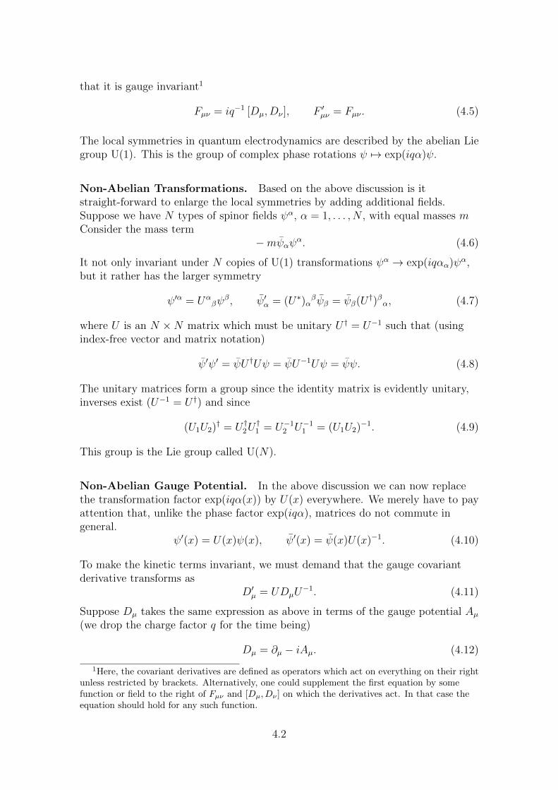
that it is gauge invariant1

Fµν = iq−1 [Dµ, Dν ], F ′µν = Fµν . (4.5)

The local symmetries in quantum electrodynamics are described by the abelian Liegroup U(1). This is the group of complex phase rotations ψ 7→ exp(iqα)ψ.

Non-Abelian Transformations. Based on the above discussion is itstraight-forward to enlarge the local symmetries by adding additional fields.Suppose we have N types of spinor fields ψα, α = 1, . . . , N , with equal masses mConsider the mass term

−mψαψα. (4.6)

It not only invariant under N copies of U(1) transformations ψα → exp(iqαα)ψα,but it rather has the larger symmetry

ψ′α = Uαβψ

β, ψ′α = (U∗)αβψβ = ψβ(U †)βα, (4.7)

where U is an N ×N matrix which must be unitary U † = U−1 such that (usingindex-free vector and matrix notation)

ψ′ψ′ = ψU †Uψ = ψU−1Uψ = ψψ. (4.8)

The unitary matrices form a group since the identity matrix is evidently unitary,inverses exist (U−1 = U †) and since

(U1U2)† = U †2U†1 = U−1

2 U−11 = (U1U2)−1. (4.9)

This group is the Lie group called U(N).

Non-Abelian Gauge Potential. In the above discussion we can now replacethe transformation factor exp(iqα(x)) by U(x) everywhere. We merely have to payattention that, unlike the phase factor exp(iqα), matrices do not commute ingeneral.

ψ′(x) = U(x)ψ(x), ψ′(x) = ψ(x)U(x)−1. (4.10)

To make the kinetic terms invariant, we must demand that the gauge covariantderivative transforms as

D′µ = UDµU−1. (4.11)

Suppose Dµ takes the same expression as above in terms of the gauge potential Aµ(we drop the charge factor q for the time being)

Dµ = ∂µ − iAµ. (4.12)

1Here, the covariant derivatives are defined as operators which act on everything on their rightunless restricted by brackets. Alternatively, one could supplement the first equation by somefunction or field to the right of Fµν and [Dµ, Dν ] on which the derivatives act. In that case theequation should hold for any such function.

4.2

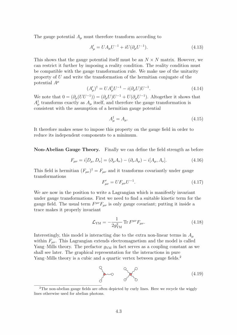
The gauge potential Aµ must therefore transform according to

A′µ = UAµU−1 + iU(∂µU

−1). (4.13)

This shows that the gauge potential itself must be an N ×N matrix. However, wecan restrict it further by imposing a reality condition. The reality condition mustbe compatible with the gauge transformation rule. We make use of the unitarityproperty of U and write the transformation of the hermitian conjugate of thepotential Aµ

(A′µ)† = UA†µU−1 − i(∂µU)U−1. (4.14)

We note that 0 = (∂µ(UU−1)) = (∂µU)U−1 + U(∂µU−1). Altogether it shows that

A†µ transforms exactly as Aµ itself, and therefore the gauge transformation isconsistent with the assumption of a hermitian gauge potential

A†µ = Aµ. (4.15)

It therefore makes sense to impose this property on the gauge field in order toreduce its independent components to a minimum.

Non-Abelian Gauge Theory. Finally we can define the field strength as before

Fµν = i[Dµ, Dν ] = (∂µAν)− (∂νAµ)− i[Aµ, Aν ]. (4.16)

This field is hermitian (Fµν)† = Fµν and it transforms covariantly under gauge

transformationsF ′µν = UFµνU

−1. (4.17)

We are now in the position to write a Lagrangian which is manifestly invariantunder gauge transformations. First we need to find a suitable kinetic term for thegauge field. The usual term F µνFµν is only gauge covariant; putting it inside atrace makes it properly invariant

LYM = − 1

2g2YM

TrF µνFµν . (4.18)

Interestingly, this model is interacting due to the extra non-linear terms in Aµwithin Fµν . This Lagrangian extends electromagnetism and the model is calledYang–Mills theory. The prefactor gYM in fact serves as a coupling constant as weshall see later. The graphical representation for the interactions in pureYang–Mills theory is a cubic and a quartic vertex between gauge fields.2

(4.19)

2The non-abelian gauge fields are often depicted by curly lines. Here we recycle the wigglylines otherwise used for abelian photons.

4.3

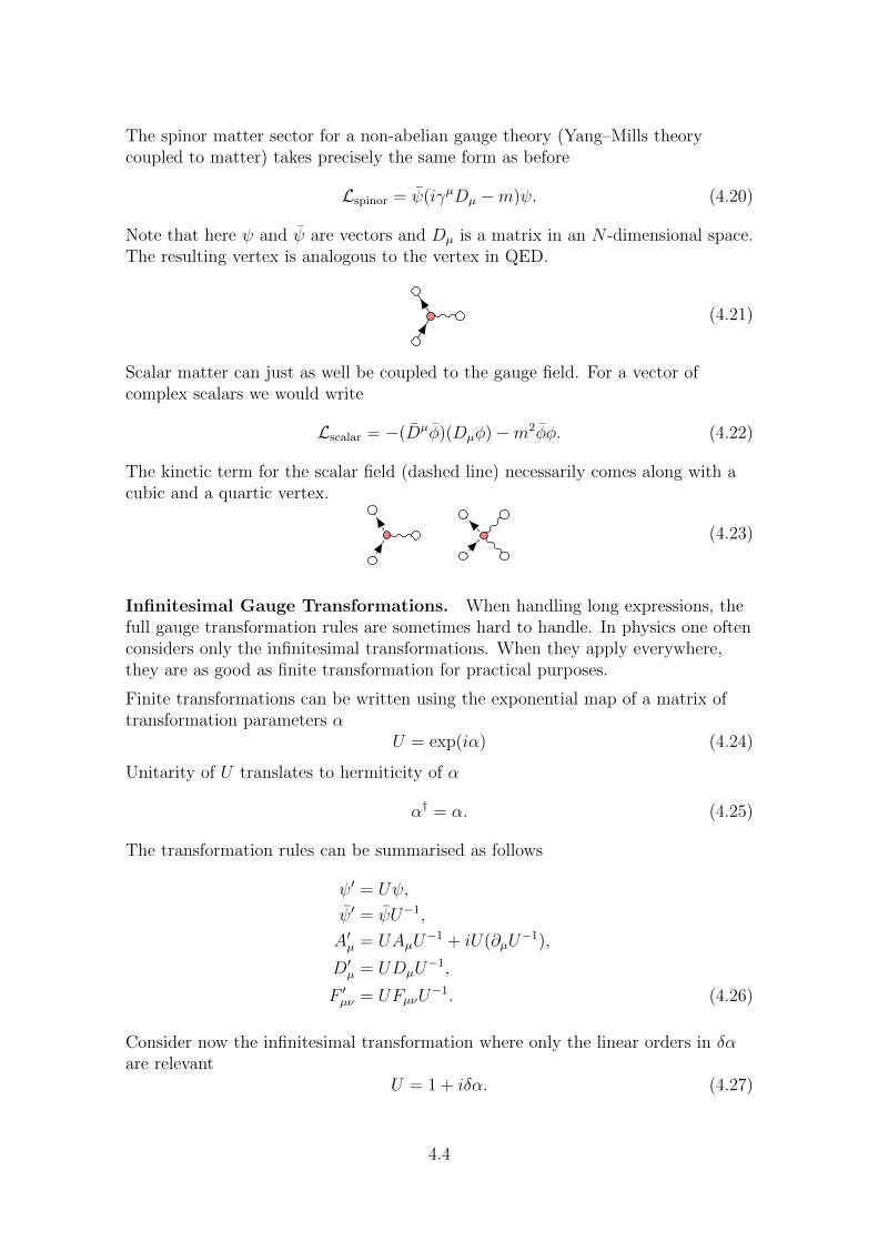
The spinor matter sector for a non-abelian gauge theory (Yang–Mills theorycoupled to matter) takes precisely the same form as before

Lspinor = ψ(iγµDµ −m)ψ. (4.20)

Note that here ψ and ψ are vectors and Dµ is a matrix in an N -dimensional space.The resulting vertex is analogous to the vertex in QED.

(4.21)

Scalar matter can just as well be coupled to the gauge field. For a vector ofcomplex scalars we would write

Lscalar = −(Dµφ)(Dµφ)−m2φφ. (4.22)

The kinetic term for the scalar field (dashed line) necessarily comes along with acubic and a quartic vertex.

(4.23)

Infinitesimal Gauge Transformations. When handling long expressions, thefull gauge transformation rules are sometimes hard to handle. In physics one oftenconsiders only the infinitesimal transformations. When they apply everywhere,they are as good as finite transformation for practical purposes.

Finite transformations can be written using the exponential map of a matrix oftransformation parameters α

U = exp(iα) (4.24)

Unitarity of U translates to hermiticity of α

α† = α. (4.25)

The transformation rules can be summarised as follows

ψ′ = Uψ,

ψ′ = ψU−1,

A′µ = UAµU−1 + iU(∂µU

−1),

D′µ = UDµU−1,

F ′µν = UFµνU−1. (4.26)

Consider now the infinitesimal transformation where only the linear orders in δαare relevant

U = 1 + iδα. (4.27)

4.4

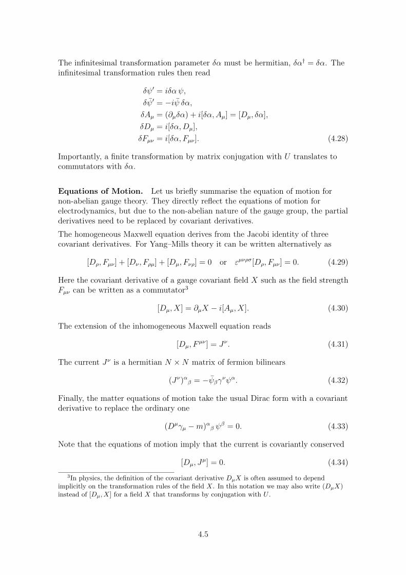
The infinitesimal transformation parameter δα must be hermitian, δα† = δα. Theinfinitesimal transformation rules then read

δψ′ = iδα ψ,

δψ′ = −iψ δα,δAµ = (∂µδα) + i[δα,Aµ] = [Dµ, δα],

δDµ = i[δα,Dµ],

δFµν = i[δα, Fµν ]. (4.28)

Importantly, a finite transformation by matrix conjugation with U translates tocommutators with δα.

Equations of Motion. Let us briefly summarise the equation of motion fornon-abelian gauge theory. They directly reflect the equations of motion forelectrodynamics, but due to the non-abelian nature of the gauge group, the partialderivatives need to be replaced by covariant derivatives.

The homogeneous Maxwell equation derives from the Jacobi identity of threecovariant derivatives. For Yang–Mills theory it can be written alternatively as

[Dρ, Fµν ] + [Dν , Fρµ] + [Dµ, Fνρ] = 0 or εµνρσ[Dρ, Fµν ] = 0. (4.29)

Here the covariant derivative of a gauge covariant field X such as the field strengthFµν can be written as a commutator3

[Dµ, X] = ∂µX − i[Aµ, X]. (4.30)

The extension of the inhomogeneous Maxwell equation reads

[Dµ, Fµν ] = Jν . (4.31)

The current Jν is a hermitian N ×N matrix of fermion bilinears

(Jν)αβ = −ψβγνψα. (4.32)

Finally, the matter equations of motion take the usual Dirac form with a covariantderivative to replace the ordinary one

(Dµγµ −m)αβ ψβ = 0. (4.33)

Note that the equations of motion imply that the current is covariantly conserved

[Dµ, Jµ] = 0. (4.34)

3In physics, the definition of the covariant derivative DµX is often assumed to dependimplicitly on the transformation rules of the field X. In this notation we may also write (DµX)instead of [Dµ, X] for a field X that transforms by conjugation with U .

4.5

4.2 Abelian Quantisation Revisited

Before we can quantise the Yang–Mills theory, we should first discuss the pathintegral formulation of electrodynamics. In QFT I, we have noticed that gaugeinvariance makes the naive vector field propagator ill-defined. The solution was tobreak gauge invariance by adding a gauge fixing term. We will now consider howto achieve this in the path integral formulation.

Naive Path Integral. Consider the action for the electromagnetic field withsources 4

SEM[A, J ] =

∫d4x

(−1

4F µνFµν − JµAµ

). (4.35)

The action is invariant under gauge transformations

SEM[A′, J ] = SEM[A, J ], (4.36)

provided that the source field is conserved,

∂µJµ = 0. (4.37)

Naively, the path integral reads

Z[J ] =

∫DA exp(iSEM[A, J ]). (4.38)

Gauge invariance of the action implies that the integrand of the path integral isconstant along all gauge-equivalent field configurations A

Z[J ] =

∫DA exp(iSEM[A, J ])

=

(∫Dα

)·∫D[A] exp(iSEM) =∞. (4.39)

Since these gauge orbits are infinite-dimensional spaces, the path integral willformally not converge.5 In other words, the path integral over the gauge potentialA is badly over-counting the admissible field configurations. We would like todivide out the divergent integral

∫Dα over gauge orbits, and keep just the integral∫

D[A] over gauge equivalence classes, but a priori we do not understand how todo it in practice.

4The sources can be an external field or represent couplings to matter fields such asJµ = ψγµψ. The latter is conserved provided that the field ψ obeys the equation of motion.Strictly speaking, coupling to charged scalar fields is not of this form due to the terms quadraticin gauge fields. Nevertheless, scalar fields can be added to the action without complications aslong as the latter remains gauge invariant.

5One may of course argue that the path integral diverges anyway, but this type of divergencecan be considered worse.

4.6

Gauge Fixing. Ideally, we should count each physical configuration only once.To this end we introduce a gauge fixing condition G[A](x) = 0 where G is somefunctional that vanishes for one point in the gauge orbit. For example, we coulduse the functional map G[A](x) = ∂µAµ(x) which enforces the Lorenz gauge.6 Infact, we will use a slightly more general gauge7

G[A,Ω](x) = ∂µAµ(x)−Ω(x). (4.40)

where Ω(x) is some function that defines the gauge. This generalisation is usefulsince we have already seen in QFT I that ∂µAµ does not identically vanish in thequantum theory.

We would like to restrict the path integral by inserting a delta functional ∆∫DA∆[G[A,Ω]] exp(iSEM[A, J ]). (4.41)

However, this insertion has the undesirable feature that it is not evidently relatedto the original formulation of Z[J ]. Furthermore, the result depends on thefunctional derivative of G at 0.8

Instead, let us consider the identity9

1 =

∫Dα∆[G[A′, Ω]] Detx,y

(δG[A′, Ω](x)

δα(y)

), (4.42)

where A′ is the gauge potential A transformed by the field α

A′µ = Aµ + (∂µα). (4.43)

A convenient feature of the above gauge-fixing functional map G is that itsfunctional derivative in the determinant is independent of A, Ω and α. It simplyreads

δG[A′, Ω](x)

δα(y)= ∂2δ(x− y). (4.44)

Hence we can write the identity as

1 = Det(∂2)

∫Dα∆[G[A′, Ω]]. (4.45)

The trick used by Faddeev and Popov is to insert the identity into the originalpath integral for the electromagnetic field

Z[J ] = Det(∂2)

∫DαDA∆[G[A′, Ω]] exp(iSEM[A, J ]). (4.46)

6This condition almost fixes the gauge up to some residual gauge transformations which areacceptable.

7Other gauges are acceptable as well, but the following discussion may have to be adapted.8This is the analog of the reparametrisation rule for delta functions

δ(f(x)) = δ(x− x0)/|f ′(x0)| where f(x0) = 0.9The functional determinant is approximated by an ordinary determinant when the

coordinates x and y are discretised.

4.7

We now perform a reparametrisation of the integration variable A to transform A′

to A. This reparametrisation is both a shift and a gauge transformation, henceDA and SEM[A, J ] remain unchanged

Z[J ] = Det(∂2)

(∫Dα

)∫DA∆[G[A,Ω]] exp(iSEM[A, J ]). (4.47)

We have now separated the path integral over gauge fixed potential A from adivergent prefactor which does not depend on A.

Averaging. Now we must somehow implement the gauge-fixing delta functionalin the path integral. One option would be to solve for one component of Aµ, e.g.A0. Doing so would violate Lorentz invariance. Preserving Lorentz symmetry isone of the aims of the path integral formalism.

An alternative is to employ another trick, and integrate out Ω with a Gaussianpotential

SΩ[Ω] = − 1

2ξ

∫d4xΩ2,

∫DΩ exp(iSΩ[Ω]) = const. . (4.48)

Since Z[J ] only formally depends on Ω this merely introduces another constantfactor into the original path integral

Z[J ] ∼∫DΩDA∆[G[A,Ω]] exp(iSEM[A, J ] + iSΩ[Ω]). (4.49)

We now use the delta functional to perform the path integral over Ω and obtain

Z[J ] ∼∫DA exp(iSEM[A, J ] + iSgf [A]) (4.50)

with an additional contribution to the action

Sgf [A] = − 1

2ξ

∫d4x (∂·A)2. (4.51)

Discussion. Finally, we have recovered the Lagrangian of the electromagneticfield with the standard Lorenz gauge fixing term. Up to some infinite but constantprefactors the new path integral is equal to the original path integral

Z[J ] =

∫DA exp(iSEM[A, J ])

= const. ·∫DA exp(iSEM[A, J ] + iSgf [A]). (4.52)

Since all constant prefactor drop out of correlation function, we can use the actionwith gauge fixing term as the starting point for quantising electrodynamics.

4.8

Note, however, that the path integrals are only equivalent when the source field Jis conserved. Therefore, only correlation functions of gauge invariant combinationsof the fields are meaningful in the gauge fixed form.10

We have used a modified Lorentz gauge condition ∂·A = Ω where Ω is an auxiliarydynamical field. This field is governed by a free Lagrangian without derivativeterms which essentially force it (quantum mechanically close) to zero. There is noneed to impose the gauge condition.

The resulting Feynman propagator for the vector field in momentum space is

(GF)µν(p) =ηµν − (1− ξ)pµpν/p2

p2 − iε. (4.53)

Note that this propagator does not respect the Lorenz gauge exactly since ∂·A incorrelators yields the propagator

pν(GF)µν(p) =ξpµ

p2 − iε(4.54)

which does not vanish identically. This is an effect of the generalised Lorenz gauge.In practice, the non-vanishing does not matter since the other side of thepropagator usually couples to the source Jµ which is conserved, pµJ

µ(p) = 0.

4.3 Yang–Mills Quantisation

We are now prepared to apply to the path integral quantisation to the vector fieldsof Yang–Mills theory. Here some further complications arise due to the non-abeliannature of the gauge group. These lead to the introduction of further fields.

Some Puzzles. If we are over-confident we could now postulate the Feynmanrules for Yang–Mills theory. When reading them off from a straight-forwardnon-abelian generalisation of the above gauge fixed action,

Z[J ] = const. ·∫DA exp(iSYM[A, J ] + iSgf [A]). (4.55)

we run into some problems. These can be seen in several ways:

We can consider the process of two matter particles annihilating into two vectorparticles

= + + (4.56)

In the abelian process the resulting photons automatically have only physicalpolarisation vectors. This turns out not to hold in the non-abelian generalisation,

10Of course we may also compute more general correlation functions, but these are potentiallyunrelated to the original path integral and thus meaningless.

4.9

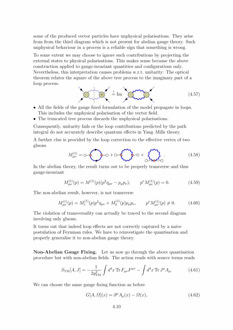
some of the produced vector particles have unphysical polarisations. They arisefrom from the third diagram which is not present for abelian gauge theory. Suchunphysical behaviour in a process is a reliable sign that something is wrong.

To some extent we may choose to ignore such contributions by projecting theexternal states to physical polarisations. This makes sense because the aboveconstruction applied to gauge-invariant quantities and configurations only.Nevertheless, this interpretation causes problems w.r.t. unitarity: The opticaltheorem relates the square of the above tree process to the imaginary part of aloop process.

∗ ?= Im (4.57)

• All the fields of the gauge fixed formulation of the model propagate in loops.This includes the unphysical polarisation of the vector field.• The truncated tree process discards the unphysical polarisations.

Consequently, unitarity fails or the loop contributions predicted by the pathintegral do not accurately describe quantum effects in Yang–Mills theory.

A further clue is provided by the loop correction to the effective vertex of twogluons

M (1)µν = + + . (4.58)

In the abelian theory, the result turns out to be properly transverse and thusgauge-invariant

M (1)µν (p) = M (1)(p)(p2ηµν − pµpν), pνM (1)

µν (p) = 0. (4.59)

The non-abelian result, however, is not transverse

M (1)µν (p) = M

(1)1 (p)p2ηµν +M

(1)2 (p)pµpν , pνM (1)

µν (p) 6= 0. (4.60)

The violation of transversality can actually be traced to the second diagraminvolving only gluons.

It turns out that indeed loop effects are not correctly captured by a naivepostulation of Feynman rules. We have to reinvestigate the quantisation andproperly generalise it to non-abelian gauge theory.

Non-Abelian Gauge Fixing. Let us now go through the above quantisationprocedure but with non-abelian fields. The action reads with source terms reads

SYM[A, J ] = − 1

2g2YM

∫d4xTrFµνF

µν −∫d4xTr JµAµ. (4.61)

We can choose the same gauge fixing function as before

G[A,Ω](x) = ∂µAµ(x)−Ω(x), (4.62)

4.10

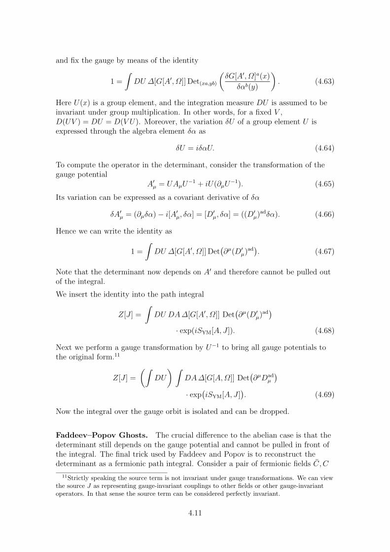
and fix the gauge by means of the identity

1 =

∫DU ∆[G[A′, Ω]] Det(xa,yb)

(δG[A′, Ω]a(x)

δαb(y)

). (4.63)

Here U(x) is a group element, and the integration measure DU is assumed to beinvariant under group multiplication. In other words, for a fixed V ,D(UV ) = DU = D(V U). Moreover, the variation δU of a group element U isexpressed through the algebra element δα as

δU = iδαU. (4.64)

To compute the operator in the determinant, consider the transformation of thegauge potential

A′µ = UAµU−1 + iU(∂µU

−1). (4.65)

Its variation can be expressed as a covariant derivative of δα

δA′µ = (∂µδα)− i[A′µ, δα] = [D′µ, δα] = ((D′µ)adδα). (4.66)

Hence we can write the identity as

1 =

∫DU ∆[G[A′, Ω]] Det

(∂µ(D′µ)ad

). (4.67)

Note that the determinant now depends on A′ and therefore cannot be pulled outof the integral.

We insert the identity into the path integral

Z[J ] =

∫DU DA∆[G[A′, Ω]] Det

(∂µ(D′µ)ad

)· exp(iSYM[A, J ]). (4.68)

Next we perform a gauge transformation by U−1 to bring all gauge potentials tothe original form.11

Z[J ] =

(∫DU

) ∫DA∆[G[A,Ω]] Det

(∂µDad

µ

)· exp

(iSYM[A, J ]

). (4.69)

Now the integral over the gauge orbit is isolated and can be dropped.

Faddeev–Popov Ghosts. The crucial difference to the abelian case is that thedeterminant still depends on the gauge potential and cannot be pulled in front ofthe integral. The final trick used by Faddeev and Popov is to reconstruct thedeterminant as a fermionic path integral. Consider a pair of fermionic fields C, C

11Strictly speaking the source term is not invariant under gauge transformations. We can viewthe source J as representing gauge-invariant couplings to other fields or other gauge-invariantoperators. In that sense the source term can be considered perfectly invariant.

4.11

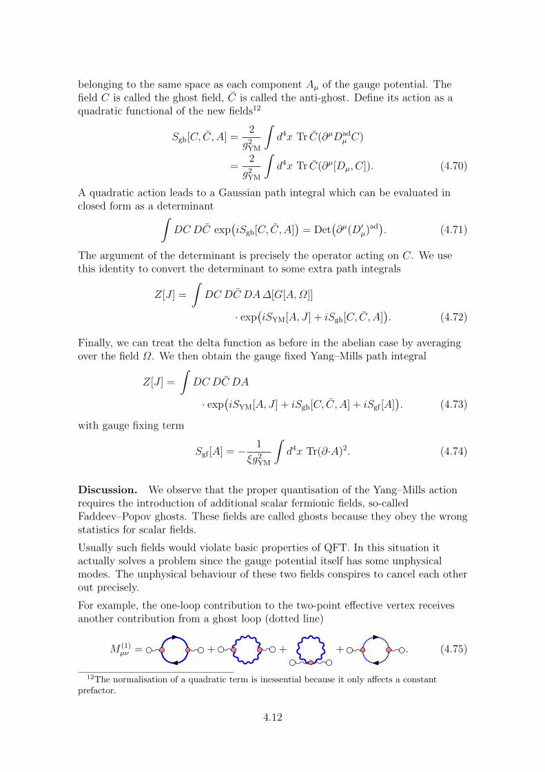
belonging to the same space as each component Aµ of the gauge potential. Thefield C is called the ghost field, C is called the anti-ghost. Define its action as aquadratic functional of the new fields12

Sgh[C, C, A] =2

g2YM

∫d4x Tr C(∂µDad

µ C)

=2

g2YM

∫d4x Tr C(∂µ[Dµ, C]). (4.70)

A quadratic action leads to a Gaussian path integral which can be evaluated inclosed form as a determinant∫

DC DC exp(iSgh[C, C, A]

)= Det

(∂µ(D′µ)ad

). (4.71)

The argument of the determinant is precisely the operator acting on C. We usethis identity to convert the determinant to some extra path integrals

Z[J ] =

∫DC DC DA∆[G[A,Ω]]

· exp(iSYM[A, J ] + iSgh[C, C, A]

). (4.72)

Finally, we can treat the delta function as before in the abelian case by averagingover the field Ω. We then obtain the gauge fixed Yang–Mills path integral

Z[J ] =

∫DC DC DA

· exp(iSYM[A, J ] + iSgh[C, C, A] + iSgf [A]

). (4.73)

with gauge fixing term

Sgf [A] = − 1

ξg2YM

∫d4x Tr(∂·A)2. (4.74)

Discussion. We observe that the proper quantisation of the Yang–Mills actionrequires the introduction of additional scalar fermionic fields, so-calledFaddeev–Popov ghosts. These fields are called ghosts because they obey the wrongstatistics for scalar fields.

Usually such fields would violate basic properties of QFT. In this situation itactually solves a problem since the gauge potential itself has some unphysicalmodes. The unphysical behaviour of these two fields conspires to cancel each otherout precisely.

For example, the one-loop contribution to the two-point effective vertex receivesanother contribution from a ghost loop (dotted line)

M (1)µν = + + + . (4.75)

12The normalisation of a quadratic term is inessential because it only affects a constantprefactor.

4.12

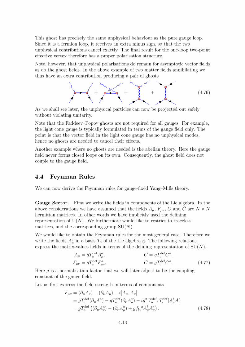
This ghost has precisely the same unphysical behaviour as the pure gauge loop.Since it is a fermion loop, it receives an extra minus sign, so that the twounphysical contributions cancel exactly. The final result for the one-loop two-pointeffective vertex therefore has a proper polarisation structure.

Note, however, that unphysical polarisations do remain for asymptotic vector fieldsas do the ghost fields. In the above example of two matter fields annihilating wethus have an extra contribution producing a pair of ghosts

+ + + (4.76)

As we shall see later, the unphysical particles can now be projected out safelywithout violating unitarity.

Note that the Faddeev–Popov ghosts are not required for all gauges. For example,the light cone gauge is typically formulated in terms of the gauge field only. Thepoint is that the vector field in the light cone gauge has no unphysical modes,hence no ghosts are needed to cancel their effects.

Another example where no ghosts are needed is the abelian theory. Here the gaugefield never forms closed loops on its own. Consequently, the ghost field does notcouple to the gauge field.

4.4 Feynman Rules

We can now derive the Feynman rules for gauge-fixed Yang–Mills theory.

Gauge Sector. First we write the fields in components of the Lie algebra. In theabove considerations we have assumed that the fields Aµ, Fµν , C and C are N ×Nhermitian matrices. In other words we have implicitly used the definingrepresentation of U(N). We furthermore would like to restrict to tracelessmatrices, and the corresponding group SU(N).

We would like to obtain the Feynman rules for the most general case. Therefore wewrite the fields Aaµ in a basis Ta of the Lie algebra g. The following relationsexpress the matrix-values fields in terms of the defining representation of SU(N).

Aµ = gT defa Aaµ, C = gT def

a Ca,

Fµν = gT defa F a

µν , C = gT defa Ca. (4.77)

Here g is a normalisation factor that we will later adjust to be the couplingconstant of the gauge field.

Let us first express the field strength in terms of components

Fµν = (∂µAν)− (∂νAµ)− i[Aµ, Aν ]= gT def

a (∂µAaν)− gT def

a (∂νAaµ)− ig2[T def

b , T defc ]AbµA

cν

= gT defa

((∂µA

aν)− (∂νA

aµ) + gfbc

aAbµAcν

). (4.78)

4.13

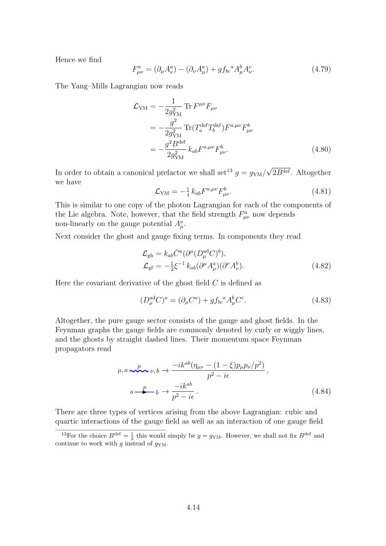
Hence we findF aµν = (∂µA

aν)− (∂νA

aµ) + gfbc

aAbµAcν . (4.79)

The Yang–Mills Lagrangian now reads

LYM = − 1

2g2YM

TrF µνFµν

= − g2

2g2YM

Tr(T defa T def

b )F a,µνF bµν

= −g2Bdef

2g2YM

kabFa,µνF b

µν . (4.80)

In order to obtain a canonical prefactor we shall set13 g = gYM/√

2Bdef . Altogetherwe have

LYM = −14kabF

a,µνF bµν . (4.81)

This is similar to one copy of the photon Lagrangian for each of the components ofthe Lie algebra. Note, however, that the field strength F a

µν now dependsnon-linearly on the gauge potential Aaµ.

Next consider the ghost and gauge fixing terms. In components they read

Lgh = kabCa(∂µ(Dad

µ C)b),

Lgf = −12ξ−1 kab(∂

µAaµ)(∂νAbν). (4.82)

Here the covariant derivative of the ghost field C is defined as

(Dadµ C)a = (∂µC

a) + gfbcaAbµC

c. (4.83)

Altogether, the pure gauge sector consists of the gauge and ghost fields. In theFeynman graphs the gauge fields are commonly denoted by curly or wiggly lines,and the ghosts by straight dashed lines. Their momentum space Feynmanpropagators read

µ, a ν, bp → −ik

ab(ηµν − (1− ξ)pµpν/p2)

p2 − iε,

a bp → −ikab

p2 − iε. (4.84)

There are three types of vertices arising from the above Lagrangian: cubic andquartic interactions of the gauge field as well as an interaction of one gauge field

13For the choice Bdef = 12 this would simply be g = gYM. However, we shall not fix Bdef and

continue to work with g instead of gYM.

4.14

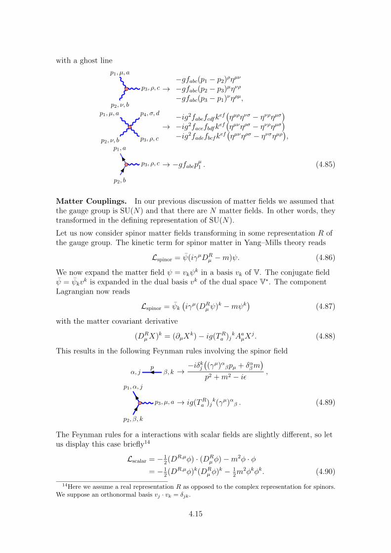
with a ghost line

p3, ρ, c

p1, µ, a

p2, ν, b

→−gfabc(p1 − p2)ρηµν

−gfabc(p2 − p3)µηνρ

−gfabc(p3 − p1)νηρµ,

p3, ρ, c

p4, σ, dp1, µ, a

p2, ν, b

→−ig2fabefcdfk

ef(ηµρηνσ − ηνρηµσ

)−ig2facefbdfk

ef(ηµνηρσ − ηνρηµσ

)−ig2fadefbcfk

ef(ηµνηρσ − ηνσηµρ

),

p3, ρ, c

p1, a

p2, b

→ −gfabcpµ1 . (4.85)

Matter Couplings. In our previous discussion of matter fields we assumed thatthe gauge group is SU(N) and that there are N matter fields. In other words, theytransformed in the defining representation of SU(N).

Let us now consider spinor matter fields transforming in some representation R ofthe gauge group. The kinetic term for spinor matter in Yang–Mills theory reads

Lspinor = ψ(iγµDRµ −m)ψ. (4.86)

We now expand the matter field ψ = vkψk in a basis vk of V. The conjugate field

ψ = ψkvk is expanded in the dual basis vk of the dual space V∗. The component

Lagrangian now reads

Lspinor = ψk(iγµ(DR

µψ)k −mψk)

(4.87)

with the matter covariant derivative

(DRµX)k = (∂µX

k)− ig(TRa )jkAaµX

j. (4.88)

This results in the following Feynman rules involving the spinor field

α, j β, kp →

−iδkj((γµ)αβpµ + δαβm

)p2 +m2 − iε

,

p3, µ, a

p1, α, j

p2, β, k

→ ig(TRa )jk(γµ)αβ . (4.89)

The Feynman rules for a interactions with scalar fields are slightly different, so letus display this case briefly14

Lscalar = −12(DR,µφ) · (DR

µ φ)−m2φ · φ= −1

2(DR,µφ)k(DR

µ φ)k − 12m2φkφk. (4.90)

14Here we assume a real representation R as opposed to the complex representation for spinors.We suppose an orthonormal basis vj · vk = δjk.

4.15

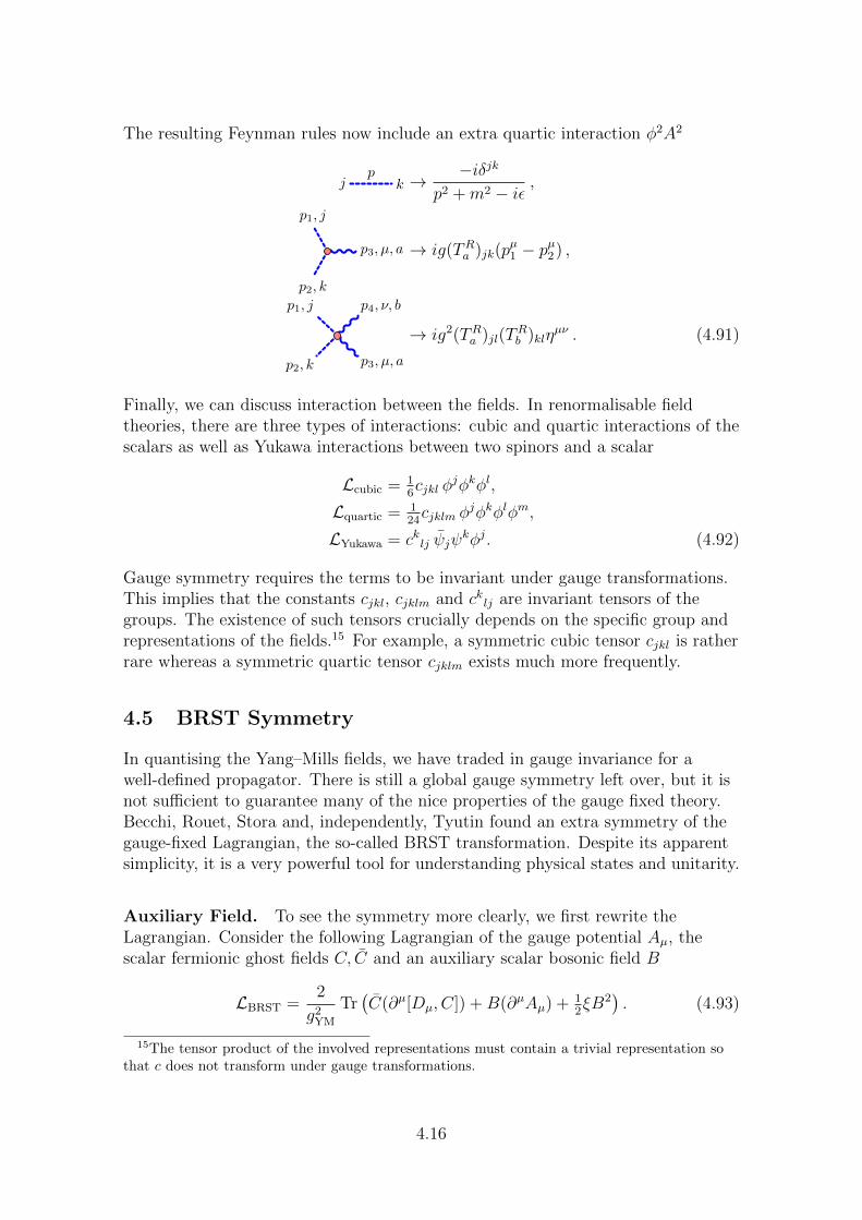
The resulting Feynman rules now include an extra quartic interaction φ2A2

j kp → −iδjk

p2 +m2 − iε,

p3, µ, a

p1, j

p2, k

→ ig(TRa )jk(pµ1 − p

µ2) ,

p3, µ, a

p4, ν, bp1, j

p2, k

→ ig2(TRa )jl(TRb )klη

µν . (4.91)

Finally, we can discuss interaction between the fields. In renormalisable fieldtheories, there are three types of interactions: cubic and quartic interactions of thescalars as well as Yukawa interactions between two spinors and a scalar

Lcubic = 16cjkl φ

jφkφl,

Lquartic = 124cjklm φ

jφkφlφm,

LYukawa = cklj ψjψkφj. (4.92)

Gauge symmetry requires the terms to be invariant under gauge transformations.This implies that the constants cjkl, cjklm and cklj are invariant tensors of thegroups. The existence of such tensors crucially depends on the specific group andrepresentations of the fields.15 For example, a symmetric cubic tensor cjkl is ratherrare whereas a symmetric quartic tensor cjklm exists much more frequently.

4.5 BRST Symmetry

In quantising the Yang–Mills fields, we have traded in gauge invariance for awell-defined propagator. There is still a global gauge symmetry left over, but it isnot sufficient to guarantee many of the nice properties of the gauge fixed theory.Becchi, Rouet, Stora and, independently, Tyutin found an extra symmetry of thegauge-fixed Lagrangian, the so-called BRST transformation. Despite its apparentsimplicity, it is a very powerful tool for understanding physical states and unitarity.

Auxiliary Field. To see the symmetry more clearly, we first rewrite theLagrangian. Consider the following Lagrangian of the gauge potential Aµ, thescalar fermionic ghost fields C, C and an auxiliary scalar bosonic field B

LBRST =2

g2YM

Tr(C(∂µ[Dµ, C]) +B(∂µAµ) + 1

2ξB2

). (4.93)

15The tensor product of the involved representations must contain a trivial representation sothat c does not transform under gauge transformations.

4.16

The field B is free and can be integrated out exactly by replacing it by its saddlepoint solution B = −ξ−1∂µAµ. This yields precisely the gauge-fixing and ghostterms

LBRST '2

g2YM

Tr(C(∂µ[Dµ, C])− 1

2ξ−1(∂µAµ)2

). (4.94)

BRST Transformation. The BRST transformation is defined as the followingvariation of the fields

δAµ = δε[Dµ, C],

δC = iδεCC = − i2δεC,C,

δC = −δεB,δB = 0. (4.95)

Note that the transformation parameter δε must be a fermionic number in order tomatch the statistics on both sides of the equation. It is straight-forward to confirmthat the Lagrangian is invariant under the BRST transformation

δLBRST = 0. (4.96)

Likewise, the Yang–Mills Lagrangian LYM is invariant since the BRSTtransformation on the ordinary fields is a plain gauge transformation withtransformation parameter εC.

Let us write the BRST transformation as a fermionic operator Q such that

δ = δεQ. (4.97)

This BRST operator has the important property that it is nilpotent

Q2 = 0, (4.98)

as can be verified easily by acting with Q2 on all fields. In fact we can write theBRST Lagrangian as a BRST variation of some other function KBRST

LBRST = QKBRST, KBRST =2

g2YM

Tr(−C(∂µAµ)− 1

2ξCB

). (4.99)

It is then evident that QLBRST = Q2KBRST = 0. The Yang–Mills Lagrangian, onthe other hand, cannot be written as a BRST variation of something, since thegauge field strength Fµν is never produced by the action of Q

LYM 6= QKYM. (4.100)

Another new symmetry is the ghost number Ngh. It counts the number of ghostsC minus the number of anti-ghosts C. The gauge and auxiliary fields carry noghost number.

4.17

BRST Cohomology. The BRST operator Q squares to zero, Q2 = 0, in closeanalogy to the exterior derivative d. Such operators define a cohomology whichoften encodes some important information. For example, the de Rham cohomologyof the exterior derivative probes the global topology of differentiable manifolds.The BRST cohomology turns out to describe physical states and operators.

Suppose we go back to canonical quantisation with a Hilbert space H. The BRSTsymmetry leads to an associated operator Q acting on H. There are two types ofdistinguished states:

• Closed states are annihilated by Q

Q|Ψ〉 = 0 ↔ |Ψ〉 ∈ Hcl. (4.101)

• Exact states are in the image of Q

|Ψ〉 = Q|Ω〉 for some |Ω〉 ∈ H ↔ |Ψ〉 ∈ Hex. (4.102)

By construction exact states are also closed, but not necessarily vice versa,Hex ⊂ Hcl. The BRST cohomology Hphys is defined as the quotient space

Hphys = Hcl/Hex. (4.103)

This space (restricted to ghost number zero) turns out to define the physicalstates. In other words, physical states are defined as equivalence classes |Ψ〉+QHof states in the original Hilbert space

|Ψ〉 ' |Ψ〉+Q|Ω〉 with Q|Ψ〉 = 0. (4.104)

We have postulated that the BRST cohomology (of ghost number zero) definesphysical states. This makes sense only if physical answers depend on equivalenceclasses but not on their representatives. The discussion is similar to thecorresponding discussion of equivalence classes of the vector field in QFT I.

The key insight is that the BRST operator is hermitian

Q† = Q. (4.105)

This implies that exact states |Ψ〉 = Q|Ω〉 have zero overlap with closed states |Φ〉

〈Φ|Ψ〉 = 〈Φ|Q|Ω〉 = 〈Φ|Q†|Ω〉 = 0. (4.106)

Therefore the scalar product is independent of the representative|Ψ ′〉 = |Ψ〉+Q|Ω〉 of an equivalence class

〈Φ|Ψ ′〉 = 〈Φ|Ψ〉+ 〈Φ|Q|Ω〉 = 〈Φ|Ψ〉. (4.107)

One-Particle States. Evidently, we should choose a vacuum state |0〉 in theBRST cohomology. As we will not define the vacuum state explicitly, we cannotdiscuss its BRST properties in detail.

Next, let us confirm that single-particle states in the BRST cohomology are indeedthe physical excitations of a vector field:

4.18

• The BRST operator maps C to B. Hence the anti-ghost field C is not closed.16

• In momentum space Aµ(p) is mapped to pµC(p).17 Thus one of the four modesof Aµ is not closed.• The image of C is the field B. Hence B is exact. Moreover, the equations of

motion identify the auxiliary field B(p) with pµAµ(p). Therefore one of the fourmodes of Aµ is exact on shell. It is different from the mode which is not closedsince exact states are closed by construction.• The image of Aµ is the ghost field. Therefore the ghost field C is exact.• The two remaining polarisation modes of the field Aµ are closed and but not

exact.

We observe that the anti-ghost C and one of the modes of Aµ are not closed andtherefore not physical. Furthermore the ghost C and another mode of Aµ are exactand therefore equivalent to the trivial state in Hphys. The two remaining modes ofAµ are physical because they are closed but not exact. These are precisely the twohelicity modes of the massless vector field.

We conclude that the cohomology for one-particle particles describes correctly theset of physical particles. The discussion for higher number of particles is not asstraight-forward due to non-linear effects.

S-Matrix Consistency. A related issue is unitarity of the physical scatteringmatrix. The BRST operator is a symmetry; therefore it commutes with theHamiltonian and with the S-matrix18

[Q,S] = 0. (4.108)

Consider some physical initial state |Ψ〉. It is scattered to a final state S|Ψ〉 whichis closed

QS|Ψ〉 = SQ|Ψ〉 = 0. (4.109)

As expected, changing the representative of the initial state changes therepresentative of the final state

S|Ψ ′〉 = S|Ψ〉+ SQ|Ω〉 = S|Ψ〉+QS|Ω〉. (4.110)

We can now consider unitarity of the S-matrix

S†S = 1. (4.111)

The optical theorem is the formulation of this statement in terms of the matrixelements of S. We enclose the unitarity statement in physical states

〈Φ|S†S|Ψ〉 = 〈Φ|Ψ〉. (4.112)

At this point we should insert the decomposition of unity between the S-matrices.A priori we should insert the unit operator on the full Hilbert space H. Using our

16And it evidently cannot be made closed in any linear combination of single-particle states.17For the discussion of single-particle states we ignore the terms non-linear in the fields.18Also the ghost number operators Ngh is a symmetry.

4.19

scalar product this is non-trivial since we know that the space Hex is null. Its dualwithin H is the quotient space H/Hcl.

19 The decomposition thus has be writtenusing some map ∗ which interchanges Hex with H/Hcl and leaves the residualphysical space Hcl/Hex = Hphys invariant

1 =∑Ω

|Ω∗〉〈Ω|

=∑

Ω physical

|Ω〉〈Ω|+∑

Ω exact

|Ω∗〉〈Ω|+∑

Ω exact

|Ω〉〈Ω∗|. (4.113)

This somewhat unusual decomposition of unity is very convenient since all theexact states are cancelled by either 〈Φ|S† or S|Ψ〉.20 The optical theorem can thusbe expressed as

〈Φ|S†S|Ψ〉 =∑

Ω physical

〈Φ|S†|Ω〉〈Ω|S|Ψ〉 = 〈Φ|Ψ〉. (4.114)

In the optical theorem one is therefore free restrict the sum to physicalintermediate states. However, one can also perform the sum over all intermediatestates including unphysical ones. The result was shown to be the same, thereforethe contributions from unphysical modes of the gauge field must cancel exactlyagainst the contributions from ghost fields. The applicability of the fullintermediate Hilbert space is crucial since unphysical gauge and ghost fieldspropagate within loops.

In conclusion, it is consistent to restrict the S-matrix to physical external states,even though loop amplitudes are computed using all the fields.

Independence of Gauge-Fixing. Finally, let us consider the relevance of thegauge fixing terms of the Lagrangian. We have already seen that LBRST is exact,LBRST = KBRST, while LYM is physical. Both terms contribute to the Hamiltonianand therefore they govern the time-evolution and scattering of states.

Consider a physical state |Ψ〉 and act with LBRST. It can be written as

LBRST|Ψ〉 = (QKBRST)|Ψ〉 = Q(KBRST|Ψ〉). (4.115)

It shows that whenever the gauge fixing term is applied to a physical state, theresult must be an exact state which is equivalent to the zero state.

This sketch of an argument demonstrates that the precise formulation of the gaugefixing does not influence the correlators of physical states. In particular allphysical correlators are independent of the parameter ξ of the Lorenz gauge.

19This is because there is exactly one exact state for every non-closed equivalence class.20Alternatively one can argue that every contribution of an exact state from one S-matrix is

cancelled by the other.

4.20

Quantum Field Theory II Chapter 5ETH Zurich, FS13 Prof. N. Beisert

19. 05. 2013

5 Renormalisation

We have touched upon loop effects, divergences and regularisation andrenormalisation at the very end of QFT I. Here we will present a broadlyapplicable regulator, apply the renormalisation to gauge theory and discuss theeffects of changing the renormalisation scale.

5.1 Dimensional Regularisation

In QFT I we have used a plain momentum cutoff to regularise some divergent loopintegrals. It served its purpose, but it is hard to define consistently for allconceivable processes, it breaks Poincare symmetry and it violates gaugesymmetry.

A modern regulator without these shortcomings is dimensional regularisation. It isbased on the fact that the degree of divergence of loop contributions stronglydepends on the dimension D of spacetime. For a sufficiently large D, every graphdevelops UV divergences (from integrating over large momenta) whereas for smallD some graphs can have IR divergences (from integrating over small or light-likemomenta). The idea of dimensional regularisation is to assume the number ofspacetime dimensions D to be a continuous (real or complex) parameter. Here, thedivergences appear as poles in D at integer values.

Basic Integral. The basic integral to consider in dimensional regularisation is

In(X) =

∫−idD`(2π)D

1

(`2 +X − iε)n. (5.1)

For convenience, we first Wick rotate the integral

In(X) =

∫dD`E

(2π)D1

(`2E +X − iε)n

. (5.2)

Now the integrand is spherically symmetric, therefore we transform to sphericalcoordinates

In(X) = Vol(SD−1)

∫ ∞0

d`E

(2π)D`D−1

E

(`2E +X − iε)n

. (5.3)

The volume of a (D − 1) sphere equals Vol(SD−1) = 2πD/2/Γ(D/2). Theremaining radial integral after a change of variables `2

E = z is a Beta function

1

2

∫ ∞0

dz

(2π)DzD/2−1

(z +X − iε)n=

Γ(D/2) Γ(n−D/2)

2(2π)D Γ(n) (X − iε)n−D/2. (5.4)

5.1

Altogether the integral reads

In(X) =Γ(n−D/2)

(4π)D/2 Γ(n)

1

(X − iε)n−D/2. (5.5)

The resulting expression has the nice feature that it is defined not only for integerD, but also for continuous values of the dimensionality of spacetime. We may thususe the above formula as the definition of the integral for continuous D.1 We haveseen in QFT I that all integrals arising from Feynman diagrams can be broughtinto this form. Hence the above formula defines an extrapolation of arbitraryFeynman diagrams to non-integer dimensions.

We observe an important feature: The Gamma function in the numerator haspoles for even integers D ≥ 2n. Indeed, the integral has a UV divergence whenD ≥ 2n.2 However, for non-integer values of D, the function is perfectly finite. Soindeed we can use a continuous number of spacetime dimensions D as a regulatorfor the integral. For four-dimensional theories, a convenient choice is to take Dslightly below 4 3

D = 4− 2ε. (5.6)

Dimensional regularisation provides a finite result for arbitrary Feynman integralsat arbitrary number of loops (as long as D is not rational). Moreover it does notneed to introduce a preferred point or direction which would violate Poincaresymmetry.

Vectors and Spinors. For models with spin, we will have to deal with vectorsin the numerator of the integral, for example4

Iµn (X) =

∫−idD`(2π)D

`µ

(`2 +X − iε)n= 0 ,

Iµνn (X) =

∫−idD`(2π)D

`µ`ν

(`2 +X − iε)n. (5.7)

Evidently, the first integral vanishes because the integrand is an anti-symmetricfunction. An alternative derivation uses Lorentz symmetry: The result musttransform as a vector. However, there is no vector at our disposal after the integralis done. Hence the result must vanish. The second integral can be performed by asimilar trick: The only Lorentz-invariant bi-vector is the metric tensor ηµν , so theintegral must be proportional to it. To find the factor of proportionality, take the

1This does not imply that the formula is morally correct or unique. It is merely a convenientand smooth interpolation between integer dimensions.

2In fact, the integral diverges also for odd D, so a pole in D is a sufficient condition for adivergent integral, but not a necessary one. For instance, in odd dimensions, poles typically occuronly at even loop orders.

3A factor of 2 for ε conveniently cancels a factor of 1/2 which is often associated to D.4Note that ε as the deviation from D = 4 and in the iε prescription for propagators is clearly

distinct. Nevertheless we will use the same symbol for both objects.

5.2

trace with ηµν . This yields

Iµνn (X) =ηµν

DηρσI

ρσn (X) =

ηµν

D

(In−1(X)−XIn(X)

)=

Γ(n− 1−D/2)

2(4π)D/2 Γ(n)

ηµν

(X − iε)n−1−D/2 . (5.8)

Note that one has to pay attention to the dimensionality of vectors and matrices.For consistency all vectors should be defined in D = 4− 2ε dimensions. Likewisethe Minkowski metric must be defined in D = 4− 2ε dimensions, which impliesthat its trace equals D,5

δµµ = ηµνηµν = D = 4− 2ε. (5.9)

Although, the difference between D and 4 is small, it can be important in the caseof divergences which contribute factors of 1/(D − 4).

Furthermore, spinor models are formulated in terms of Dirac gamma matrices.Their Clifford algebra depends on the number of spacetime dimensions, and forconsistency, this should also equal D. The spinor representation growsexponentially with D, so for evaluating a trivial trace we must set

Tr 1 = 2D/2. (5.10)

Everything else must be derived strictly from the Clifford algebra relation

γµ, γν = −2ηµν . (5.11)

For instance, some of the bracketing identities generalise as

γµγµ = 12γµ, γµ = −D,

γµγνγµ = γµ, γνγµ − γνγµγµ = (D − 2)γν . (5.12)

A complication of dimensional regularisation is that there is no universalgeneralisation of the totally antisymmetric tensor εµνρσ in continuous dimensionsD. For spinors it means that the additional gamma matrix γ5 does not existimmediately. This shortcoming is related to important physical effects such asanomalies of quantum symmetries. A cure to this problem is to formally introducean antisymmetric tensor εµνρσ with6

ε0123 = +1. (5.13)

The resulting matrix γ5 is then similar to the usual γ5 in four dimensions, but ithas slightly different algebraic properties, which become relevant in connection todivergences.

5At the end of the day, the external momentum vectors will be defined in exactly fourdimensions, which may lead to some confusion.

6Strictly speaking this requires D ≥ 4, but we may assume ε < 0.

5.3

Introduction of a Scale. Let us consider a simple QFT model in dimensionalregularisation. For example, the Lagrangian of a scalar with a quartic interactionreads

L = −12(∂φ)2 − 1

2m2φ2 − 1

24λφ4. (5.14)

Consider now the mass dimension. For D = 4, φ,m, ∂ all have unit massdimension and λ is a dimensionless quantity. All terms in the Lagrangian havemass dimension 4 so that the action is properly dimensionless.

In dimensional regularisation there are two choices to obtain a dimensionlessaction S =

∫dDxL:

• We can keep the dimension of all involved quantities fixed. Then we have tomultiply the Lagrangian by some overall dimensionful factor

L = µ−2ε(−1

2(∂φ)2 − 1

2m2φ2 − 1

24λφ4). (5.15)

Here µ is some regularisation constant with unit mass dimension.• The alternative is to adjust the mass dimension of the field φ to 1− ε. Then the

kinetic terms have the desired mass dimension 4− 2ε. The interaction term,however, has mass dimension 4− 4ε. We can compensate it either by attributinga mass dimension 2ε to λ, or by factoring out this mass dimension and keeping λdimensionless

L = −12(∂φ)2 − 1

2m2φ2 − 1

24µ2ελφ4. (5.16)

Note that both choices are equivalent up to a rescaling of the field φ by µε.

In the first choice, µ−2ε is an overall prefactor of the action. It acts like Planck’sconstant 1/~ which we have already observed to count loops in Feynman graphs.A contribution at L loops therefore comes along with a factor of

λL µ2εL. (5.17)

This is in fact the only place where the new scale can appear. The dependence onµ therefore is always very mild since its exponent ε is always very small. It islogarithmic rather than polynomial.

Expansion. Consider the standard massive scalar bubble integral

I =

=µ2ε

2

∫−idD`(2π)D

1

`2 +m2 − iε1

(p− `)2 +m2 − iε

=µ2ε

2

∫ 1

0

dz

∫−idD`(2π)D

1

(`2 + zzp2 +m2 − iε)2 . (5.18)

In the second step we have combined the denominators and shifted the integrationvariable to centre the integrand. The integral has the desired form and we use thedimensionally regulated expression

I =Γ(ε)

32π2

∫ 1

0

dz

(zzp2 +m2 − iε

4πµ2

)−ε. (5.19)

5.4

Next we expand the integrand in ε 7

I =1

32π2

∫ 1

0

dz

(1

ε− γE − log

zzp2 +m2 − iε4πµ2

+O(ε)

). (5.20)

We have performed the relevant parts of this integral in QFT I, here we obtain

I = − 1

16π2

√p2 + 4m2 − iε

−p2arctan

√−p2

p2 + 4m2 − iε

+1

32π2

(1

ε− γE + log(4π) + 2− log

m2

µ2

)+O(ε) . (5.21)

The dimensional regularisation agrees with the cut-off scheme up to terms of orderε and up to some constant shifts. The constant shifts can actually be absorbed byan appropriate change of the renormalisation scale µ. Alternatively, they can becancelled directly by counterterms. One of these shift terms is a pole at ε = 0which indicates the divergence in D = 4. Such poles are typical for dimensionalregularisation.

We have terminated the expansion at ε0. This makes sense since we are mainlyinterested in the physics in D = 4. What about the terms at positive orders of ε?Are they relevant? Yes and no!

• Some of the sub-leading terms in ε are required even at D = 4. This is the casewhenever there are divergences in the Feynman diagram that can undo thesuppression of O(ε) terms.• The higher-order terms in ε typically have a more complicated structure which is

reminiscent of higher-loop contributions. In fact they compete with higher-loopterms and all terms are necessary to construct a consistent final result.• After all divergences have been removed, we will eventually set ε = 0 and thus

drop these terms.• Note that setting ε = 0 too early may discard some essential terms from the final

answer and make it inconsistent. For example, the external states in a scatteringprocess are usually defined in D = 4. However, this may lead to violations ofunitarity since it is conceivable that the corresponding integrals over the phasespace of intermediate particles diverge. In those cases, the difference between asimplified phase space with D = 4 and the actual phase space with D = 4− 2εmay be important.

5.2 Renormalisation

Dimensional regularisation makes Feynman integrals finite at the cost ofintroducing a regularisation parameter ε and a regularisation scale µ. Thephysically relevant model is at ε = 0, but we cannot send ε to zero as typicalresults have some singularity at ε = 0. We first need to remove these singularitiesby redefining the parameters and fields of the model. This allows to remove the

7Integration and expansion do not necessarily always commute, but here it is not a problem.

5.5

regulator by sending ε→ 0 and recover physically meaningful results. The crucialquestion is whether this so-called renormalisation procedure can render allobservables finite at the same time.

Counterterms. Consider the dimensionally regulated massive scalar bubbleintegral

I = . . .+1

32π2

(1

ε− γE + log(4π) + 2− log

m2

µ2

)+O(ε) . (5.22)

In a scalar field theory with quartic interactions it can arise as the one-loopcorrection to the quartic interaction. When cubic interactions are included it alsoserves as a one-loop correction to the cubic interaction and to the kinetic term,specifically to the mass.

These three correction terms have a simple pole at ε = 0. We can remove thedivergences by adding counterterms for the quartic interaction, the cubicinteraction and the mass. Specifically, a suitable redefinition of the quarticcoupling constant λ is8

λ′MS = λ+ 3λ2 1

32π2ε+O(λ3). (5.23)

This counterterm removes precisely the 1/ε term in the above integral. Effectively,it changes the regularised integral to the subtracted integral IMS = I − 1/32π2ε

IMS = . . .+1

32π2

(−γE + log(4π) + 2− log

m2

µ2

)+O(ε) . (5.24)

In terms of diagrams the divergent loop has a counterterm that makes it perfectlyfinite

+1

3= . (5.25)

This result can be generalised to a method of constructing minimal countertermsproportional to pole term 1/ε. In the dimensionally regularised integrals thisremoves all corresponding poles 1/ε and makes them finite. The method is calledthe minimal subtraction (MS) scheme. At one loop it can be convenientlyimplemented at the level of regularised integrals by simply discarding the 1/εterms.

Inspection of many cases makes obvious that each pole 1/ε is accompanied by anEuler constant −γE and a logarithm log(4π). Importantly they all arise in theuniversal combination 1/ε− γE + log(4π). It is therefore convenient to modify thescheme to that counterterms are proportional to this combination.

λ′MS

= λ+ 3λ2 1/ε− γE + log(4π)

32π2+O(λ3). (5.26)

8λ′MS is the bare coupling constant appearing in the Lagrangian and λ is the renormalisedcoupling.

5.6

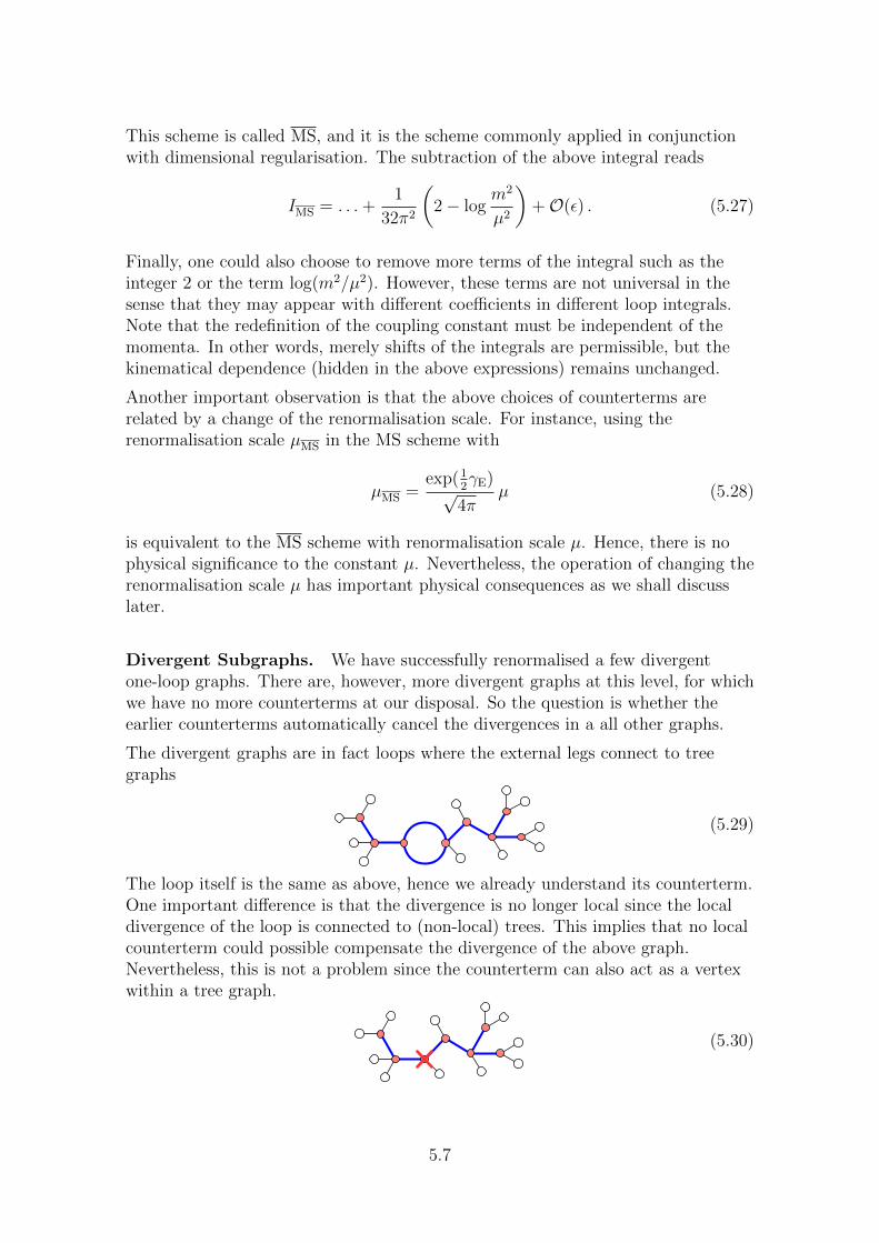
This scheme is called MS, and it is the scheme commonly applied in conjunctionwith dimensional regularisation. The subtraction of the above integral reads

IMS = . . .+1

32π2

(2− log

m2

µ2

)+O(ε) . (5.27)

Finally, one could also choose to remove more terms of the integral such as theinteger 2 or the term log(m2/µ2). However, these terms are not universal in thesense that they may appear with different coefficients in different loop integrals.Note that the redefinition of the coupling constant must be independent of themomenta. In other words, merely shifts of the integrals are permissible, but thekinematical dependence (hidden in the above expressions) remains unchanged.

Another important observation is that the above choices of counterterms arerelated by a change of the renormalisation scale. For instance, using therenormalisation scale µMS in the MS scheme with

µMS =exp(1

2γE)

√4π

µ (5.28)

is equivalent to the MS scheme with renormalisation scale µ. Hence, there is nophysical significance to the constant µ. Nevertheless, the operation of changing therenormalisation scale µ has important physical consequences as we shall discusslater.

Divergent Subgraphs. We have successfully renormalised a few divergentone-loop graphs. There are, however, more divergent graphs at this level, for whichwe have no more counterterms at our disposal. So the question is whether theearlier counterterms automatically cancel the divergences in a all other graphs.

The divergent graphs are in fact loops where the external legs connect to treegraphs

(5.29)

The loop itself is the same as above, hence we already understand its counterterm.One important difference is that the divergence is no longer local since the localdivergence of the loop is connected to (non-local) trees. This implies that no localcounterterm could possible compensate the divergence of the above graph.Nevertheless, this is not a problem since the counterterm can also act as a vertexwithin a tree graph.

(5.30)

5.7

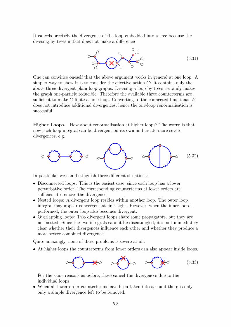
It cancels precisely the divergence of the loop embedded into a tree because thedressing by trees in fact does not make a difference

(5.31)

One can convince oneself that the above argument works in general at one loop. Asimpler way to show it is to consider the effective action G: It contains only theabove three divergent plain loop graphs. Dressing a loop by trees certainly makesthe graph one-particle reducible. Therefore the available three counterterms aresufficient to make G finite at one loop. Converting to the connected functional Wdoes not introduce additional divergences, hence the one-loop renormalisation issuccessful.

Higher Loops. How about renormalisation at higher loops? The worry is thatnow each loop integral can be divergent on its own and create more severedivergences, e.g.

(5.32)

In particular we can distinguish three different situations:

• Disconnected loops: This is the easiest case, since each loop has a lowerperturbative order. The corresponding counterterms at lower orders aresufficient to remove the divergence.• Nested loops: A divergent loop resides within another loop. The outer loop

integral may appear convergent at first sight. However, when the inner loop isperformed, the outer loop also becomes divergent.• Overlapping loops: Two divergent loops share some propagators, but they are

not nested. Since the two integrals cannot be disentangled, it is not immediatelyclear whether their divergences influence each other and whether they produce amore severe combined divergence.

Quite amazingly, none of these problems is severe at all:

• At higher loops the counterterms from lower orders can also appear inside loops.

(5.33)

For the same reasons as before, these cancel the divergences due to theindividual loops.• When all lower-order counterterms have been taken into account there is only

only a simple divergence left to be removed.

5.8

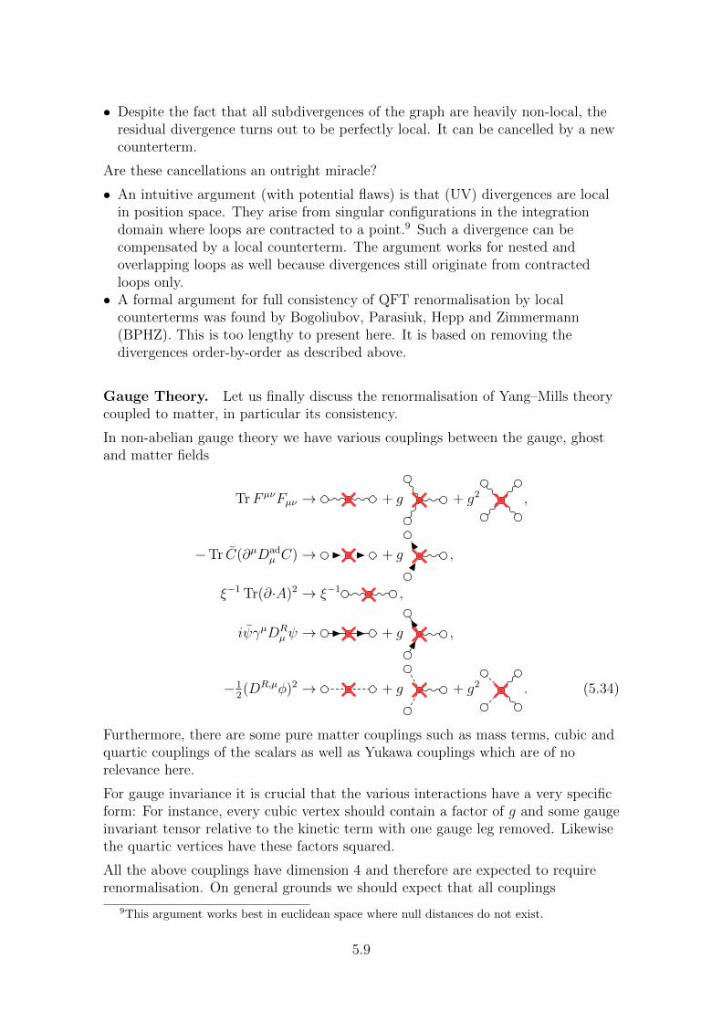
• Despite the fact that all subdivergences of the graph are heavily non-local, theresidual divergence turns out to be perfectly local. It can be cancelled by a newcounterterm.

Are these cancellations an outright miracle?

• An intuitive argument (with potential flaws) is that (UV) divergences are localin position space. They arise from singular configurations in the integrationdomain where loops are contracted to a point.9 Such a divergence can becompensated by a local counterterm. The argument works for nested andoverlapping loops as well because divergences still originate from contractedloops only.• A formal argument for full consistency of QFT renormalisation by local

counterterms was found by Bogoliubov, Parasiuk, Hepp and Zimmermann(BPHZ). This is too lengthy to present here. It is based on removing thedivergences order-by-order as described above.

Gauge Theory. Let us finally discuss the renormalisation of Yang–Mills theorycoupled to matter, in particular its consistency.

In non-abelian gauge theory we have various couplings between the gauge, ghostand matter fields

TrF µνFµν → + g + g2 ,

−Tr C(∂µDadµ C)→ + g ,

ξ−1 Tr(∂·A)2 → ξ−1 ,

iψγµDRµψ → + g ,

−12(DR,µφ)2 → + g + g2 . (5.34)

Furthermore, there are some pure matter couplings such as mass terms, cubic andquartic couplings of the scalars as well as Yukawa couplings which are of norelevance here.

For gauge invariance it is crucial that the various interactions have a very specificform: For instance, every cubic vertex should contain a factor of g and some gaugeinvariant tensor relative to the kinetic term with one gauge leg removed. Likewisethe quartic vertices have these factors squared.

All the above couplings have dimension 4 and therefore are expected to requirerenormalisation. On general grounds we should expect that all couplings

9This argument works best in euclidean space where null distances do not exist.

5.9

renormalise independently. It is conceivable that each graph may have acounterterm with an individual coefficient. This would be troublesome for tworeasons:

• At leading order all the gauge couplings were determined by a universal constantg and the discrete choice of representation. Renormalisation would introduce anindividually tunable constant for each type of field, and thus reduce thepredictive power of the model.• Gauge invariance would break down which in turn would break renormalisability

of the vector field.

Does gauge invariance survive renormalisation?

Gladly, it turns out that the above vertices renormalise coherently. The reason issymmetry. Although we had to break gauge symmetry to quantise the theory,there are two parts left.

• Manifest global symmetry under the gauge group: This symmetry ensures thatall vertices are governed by invariant tensors of the gauge group. Moreover, therelative coefficients are fixed by the Ward–Takahashi identity which is thequantum analog of the conservation of Noether currents. Therefore the couplingg acts as a universal renormalised gauge coupling constant.• BRST symmetry: This symmetry ensures that the ghosts and the unphysical

polarisations of the vector field are equivalent up to signs which make theiroverall contribution cancel exactly.

The above 5 classes of terms therefore lead to 6 independent renormalisationcoefficients:

• One renormalisation coefficient for each line.• In total one relative renormalisation coefficient for the elements in each line.

They are interpreted as follows:

• One coefficient to renormalise the kinetic term of each type of field, namely thegauge, ghost, spinor and scalar fields. These are all independent and they haveno physical relevance on their own. Nevertheless, they are important coefficientswhich contribute to each graph via the external legs.• One coefficient to (potentially) renormalise the constant ξ.• One coefficient to renormalise the gauge coupling g.

One-Loop Renormalisation in Yang–Mills Theory. Let us discuss therenormalisation of the Yang–Mills coupling g. In order to extract it, we need toconsider the kinetic term and the cubic coupling of gauge fields. For simplicity, we

5.10

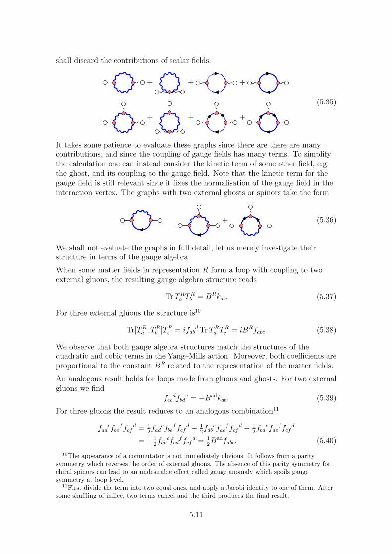
shall discard the contributions of scalar fields.

+ + +

+ + +

(5.35)

It takes some patience to evaluate these graphs since there are there are manycontributions, and since the coupling of gauge fields has many terms. To simplifythe calculation one can instead consider the kinetic term of some other field, e.g.the ghost, and its coupling to the gauge field. Note that the kinetic term for thegauge field is still relevant since it fixes the normalisation of the gauge field in theinteraction vertex. The graphs with two external ghosts or spinors take the form

+ (5.36)

We shall not evaluate the graphs in full detail, let us merely investigate theirstructure in terms of the gauge algebra.

When some matter fields in representation R form a loop with coupling to twoexternal gluons, the resulting gauge algebra structure reads

TrTRa TRb = BRkab. (5.37)

For three external gluons the structure is10

Tr[TRa , TRb ]TRc = ifab

d TrTRd TRc = iBRfabc. (5.38)

We observe that both gauge algebra structures match the structures of thequadratic and cubic terms in the Yang–Mills action. Moreover, both coefficients areproportional to the constant BR related to the representation of the matter fields.

An analogous result holds for loops made from gluons and ghosts. For two externalgluons we find

facdfbd

c = −Badkab. (5.39)

For three gluons the result reduces to an analogous combination11

fadefbe

ffcfd = 1

2fad

efbeffcf

d − 12fdb

efaeffcf

d − 12fba

efdeffcf

d

= −12fab

efedffcf

d = 12Badfabc. (5.40)

10The appearance of a commutator is not immediately obvious. It follows from a paritysymmetry which reverses the order of external gluons. The absence of this parity symmetry forchiral spinors can lead to an undesirable effect called gauge anomaly which spoils gaugesymmetry at loop level.

11First divide the term into two equal ones, and apply a Jacobi identity to one of them. Aftersome shuffling of indice, two terms cancel and the third produces the final result.

5.11

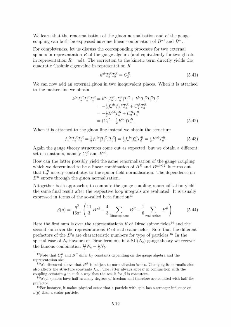
We learn that the renormalisation of the gluon normalisation and of the gaugecoupling can both be expressed as some linear combination of Bad and BR.

For completeness, let us discuss the corresponding processes for two externalspinors in representation R of the gauge algebra (and equivalently for two ghostsin representation R = ad). The correction to the kinetic term directly yields thequadratic Casimir eigenvalue in representation R

kabTRa TRb = CR

2 . (5.41)

We can now add an external gluon in two inequivalent places. When it is attachedto the matter line we obtain

kbcTRb TRa T

Rc = kbc[TRb , T

Ra ]TRc + kbcTRa T

Rb T

Rc

= −12fadcfdc

eTRe + CR2 T

Ra

= −12BadTRa + CR

2 TRa

= (CR2 − 1

2Bad)TRa . (5.42)

When it is attached to the gluon line instead we obtain the structure

fabcTRb T

Rc = 1

2fabc[TRb , T

Rc ] = i

2fabcfdbcT

Rd = i

2BadTRa . (5.43)

Again the gauge theory structures come out as expected, but we obtain a differentset of constants, namely CR

2 and Bad.

How can the latter possibly yield the same renormalisation of the gauge couplingwhich we determined to be a linear combination of BR and Bad?12 It turns outthat CR

2 merely contributes to the spinor field normalisation. The dependence onBR enters through the gluon normalisation.

Altogether both approaches to compute the gauge coupling renormalisation yieldthe same final result after the respective loop integrals are evaluated. It is usuallyexpressed in terms of the so-called beta function13

β(g) =g3

16π2

(11

3Bad − 4

3

∑Dirac spinors

BR − 1

6

∑real scalars

BR

). (5.44)

Here the first sum is over the representations R of Dirac spinor fields14 and thesecond sum over the representations R of real scalar fields. Note that the differentprefactors of the B’s are characteristic numbers for type of particles.15 In thespecial case of Nf flavours of Dirac fermions in a SU(Nc) gauge theory we recoverthe famous combination 11

3Nc − 4

3Nf .

12Note that CR2 and BR differ by constants depending on the gauge algebra and therepresentation size.

13We discussed above that BR is subject to normalisation issues. Changing its normalisationalso affects the structure constants fabc. The latter always appear in conjunction with thecoupling constant g in such a way that the result for β is consistent.

14Weyl spinors have half as many degrees of freedom and therefore are counted with half theprefactor.

15For instance, it makes physical sense that a particle with spin has a stronger influence onβ(g) than a scalar particle.

5.12

5.3 Renormalisation Flow

Physical results should not depend on the arbitrary choice of regularisation andrenormalisation scheme. However, we have already seen that the parameters ofquantum field theory models must be adjusted to the choice of renormalisationscheme in order to obtain the desired result.

Here we shall discuss the dependence of the parameters and the results on therenormalisation scheme. In particular, we have seen that the various schemesintroduce a renormalisation scale which consequently appears as a new parameterfor all results. We shall therefore discuss the dependence on it, called therenormalisation (group) flow, along with its implications for the coupling constants.

Callan–Symanzik Equation. Let us consider a simple quantum field theoryfor a single massless field φ with a single dimensionless coupling constant λ and aregularisation scale µ.16 For example, the latter can be a momentum cutoff scaleor the scale parameter of dimensional regularisation. We shall be interested inn-point correlation functions Gn in momentum space which depend on themomenta pk, as well as λ and µ

Gn(pk, λ, µ). (5.45)

Suppose we change the renormalisation scale by some amount. Then we should beable to compensate the change of any physical variable by a change of the couplingconstant and the renormalisation of the n external fields17

∂Gn

∂µ+∂λ

∂µ

∂Gn

∂λ− n

φ

∂φ

∂µGn = 0. (5.46)

It is called the Callan–Symanzik equation. It completely determines thedependence on the renormalisation scale µ and thus makes it an irrelevantparameter since every physical quantity can be computed at arbitrary µ.

The Callan–Symanzik equation has the general form(µ∂

∂µ+ β(λ)

∂

∂λ+ nγ(λ)

)Gn(pk, λ, µ) = 0. (5.47)

where we have introduced the conventional functions β(λ) and γ(λ)

β(λ) = µδλ

δµ, γ(λ) = −µ

φ

δφ

δµ. (5.48)

These dimensionless functions are universally defined for the QFT model at handindependently of the particular observable one may be interested in. Therefore

16The following discussion applies just as well for several fields with several coupling constants.Masses and dimensionful coupling constants are also welcome, but require a generaliseddiscussion in terms of conformal properties.

17This follows, for instance, from performing the rescaling in the path integral formulation ofthe generating functional.

5.13

they cannot depend on the external momenta, and since they are dimensionlessthey must depend only on λ which is the only universal dimensionless parameter ofthe model.

A useful alternative form of the Callan–Symanzik equation follows by a commonrescaling of all the momenta, fields and the renormalisation scale. Such a rescalingis trivial since there are no other scales involved in the calculation(∑

kpk

∂

∂pk− nd+ µ

∂

∂µ

)Gn = 0. (5.49)

Here d represents the canonical mass dimension of the field φ(p). Combine thiswith the Callan–Symanzik equation yields the equation(∑

kpk

∂

∂pk− β(λ)

∂

∂λ− n

(d+ γ(λ)

))Gn = 0 (5.50)

This form is useful since it tells that changing the scale of all external momenta isequivalent to

• a change of the coupling strength λ together with a• rescaling the external fields according to a deformed mass dimension d+ γ(λ).

This has some crucial physical consequences:

• The strength of the coupling constant depends on the scale of the externalmomenta. This effect is called a running coupling, and it is governed by the betafunction β(λ).• The mass dimension of the field φ effectively departs from its canonical value d

to d+ γ(λ) when interactions are turned on. This coefficient γ(λ) is called theanomalous dimension of the field φ. It is governed by renormalisation of thekinetic term, also known as wave-function renormalisation.• The running of the coupling constant can also be interpreted as an anomalous

dimension of the coupling constant. The coupling constant develops an effectivemass dimension once interactions are turned on. This effect is calleddimensional transmutation. It follows from the Callan–Symanzik equation whichessentially relates the coupling constant to the renormalisation scale, andtherefore allows us to remove the coupling constant λ in favour of the scale µ.• The anomalous dimensions of the fields and the coupling constants are directly

related to the UV divergences in QFT: They would never arise in a naivetreatment of QFT without regularisation and renormalisation. One could arguethat, since anomalous dimensions are indeed physical phenomena, a naivetreatment of QFT ends up producing infinities in response to this conflict.

Running Coupling. The Callan–Symanzik equation is particularly strong andeasiest to interpret for a two-point function G2 which depends on a singlemomentum scale p only. Equivalently we can consider a higher-point function Gfor a particular momentum configuration which is governed by a single overallmomentum scale p. The Callan–Symanzik equation thus reads(

p∂

∂p− β(λ)

∂

∂λ− nd− nγ(λ)

)G(p, λ, µ) = 0. (5.51)

5.14

Let us introduce the running coupling function λ(z, λ) with z = p/µ which isdefined by a differential equation and an initial condition(

p∂

∂p− β(λ)

∂

∂λ

)λ(p/µ, λ) = 0, λ(1, λ) = λ. (5.52)

Furthermore we make an ansatz depending on the running coupling and withappropriate overall scaling

G(p, λ, µ) = pndG(p/µ, λ(p/µ, λ)

). (5.53)

It simplifies the Callan–Symanzik equation as follows(z∂

∂z− nγ

(λ(z, λ)

))G(z, λ) = 0, (5.54)

where λ(z, λ) is the inverse function of λ(z, λ). This equation is now easy enoughto solve as

G(z, λ) = exp

(∫ z

1

dz′

z′nγ(λ(z′, λ)

))F (λ) (5.55)

with a function F (λ) to be determined by the dynamics of the QFT.

The running coupling constant λ depends on the (relative) momentum scale p/µ.However, since several particles are involved in each interaction, which momentumdoes p refer to? The momentum dependence can be interpreted in several ways:

• The elementary interaction of QED involves a single photon line. One couldargue that p is an (approximate) measure of the virtuality of this photon. Forexample, consider Z± production at a particle collider with intermediatephotons. Its virtuality (centre-of-mass energy) in the electroweak regime (100GeV) determines the effective coupling strength of the electromagnetic field.Here the effective fine structure constant is significantly different than foreveryday electromagnetic processes.In non-abelian gauge theories, the association of energy to a specific particle isnot as straight-forward since the cubic gauge vertex makes no distinctionbetween the three contributing gluons.• More accurately, the above equations hold when all the momenta involved in the

process are rescaled by exactly the same amount. Here the equations predict theshift of the coupling due to the scaling factor.• To understand the precise dependence on all involved momenta, one must

calculate the actual loop integrals.

Dimensional Regularisation. Suppose we compute some correlation functionin the dimensional regularisation scheme. The bare result G in terms of the barecoupling constant λ is expressed as G(pk, λ, µ, ε).

Now in dimensional regularisation the renormalisation scale µ appears in a verypredictable fashion: Up to some potential rescalings it only appears in thecombination λµ2ε. This combination has a non-trivial mass dimension which we

5.15

should compensate by some appropriate powers of the momenta pk. Moreover theoverall mass dimension of G is nd. We can thus write the most general result inthe following form18

G(p, λ, µ, ε) = pndF (λ(µ/p)2ε, ε). (5.56)

This function obeys the Callan–Symanzik equation with the parameters

β(λ) = −2ε λ, γ(λ) = 0. (5.57)

The non-zero beta function tells us that the coupling constant has an effectivemass dimension which tends to zero when the regulator ε is removed. The crucialpoint is that we cannot yet remove the regulator since the bare result G typicallyhas a pole at ε = 0. This calls for renormalisation

Gn(pk, λ, µ, ε) = N(λ)nGn(pk, λ(λ), µ, ε) (5.58)

The renormalised result Gn is now finite with divergences hidden in the fieldrenormalisation N(λ) and coupling constant renormalisation λ(λ).

Assuming that the Callan–Symanzik equation holds in terms of the originalvariables, the Callan–Symanzik equation also holds for the renormalised variableswith the renormalised functions

β(λ(λ)) = β(λ)∂λ

∂λ(λ),

γ(λ(λ)) = γ(λ) +β(λ)

N(λ)

∂N

∂λ(λ). (5.59)

Renormalisation therefore preserves the Callan–Symanzik equation with deformedparameters.

Suppose in dimensional regularisation the renormalisation functions take thefollowing generic form with poles at ε = 0

λ = λ+ λ2(b1/ε+ b2 + . . .) + . . . ,

λ = λ− λ2(b1/ε+ b2 + . . .) + . . . ,

N(λ) = 1 + λ(c1/ε+ c2 + . . .) + . . . . (5.60)

Substituting these into the above expressions we obtain perfectly regularexpressions for β and γ at ε→ 0

β(λ) = −2ελ− 2λ2(b1 + b2ε+ . . .) + . . . ,

γ(λ) = −2λ(c1 + c2ε+ . . .) + . . . . (5.61)

Taking the limit ε→ 0, we find the renormalised expressions

β(λ)→ −2b1λ2 + . . . , γ(λ)→ −2c1λ+ . . . . (5.62)

18For simplicity we shall not distinguish between the individual momenta pk and simply referto them by p. Additional individual momenta can be interpreted as additional scalar parameterswhich play no role for our considerations.

5.16

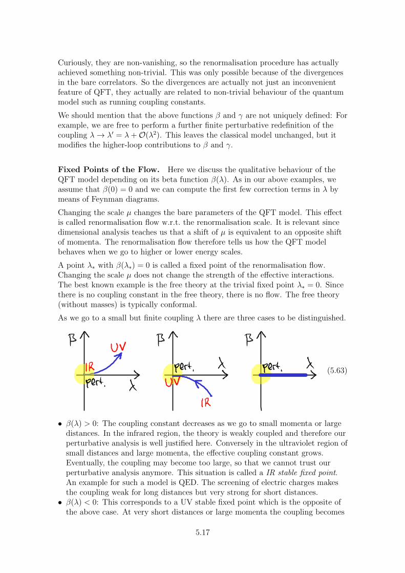
Curiously, they are non-vanishing, so the renormalisation procedure has actuallyachieved something non-trivial. This was only possible because of the divergencesin the bare correlators. So the divergences are actually not just an inconvenientfeature of QFT, they actually are related to non-trivial behaviour of the quantummodel such as running coupling constants.

We should mention that the above functions β and γ are not uniquely defined: Forexample, we are free to perform a further finite perturbative redefinition of thecoupling λ→ λ′ = λ+O(λ2). This leaves the classical model unchanged, but itmodifies the higher-loop contributions to β and γ.

Fixed Points of the Flow. Here we discuss the qualitative behaviour of theQFT model depending on its beta function β(λ). As in our above examples, weassume that β(0) = 0 and we can compute the first few correction terms in λ bymeans of Feynman diagrams.

Changing the scale µ changes the bare parameters of the QFT model. This effectis called renormalisation flow w.r.t. the renormalisation scale. It is relevant sincedimensional analysis teaches us that a shift of µ is equivalent to an opposite shiftof momenta. The renormalisation flow therefore tells us how the QFT modelbehaves when we go to higher or lower energy scales.

A point λ∗ with β(λ∗) = 0 is called a fixed point of the renormalisation flow.Changing the scale µ does not change the strength of the effective interactions.The best known example is the free theory at the trivial fixed point λ∗ = 0. Sincethere is no coupling constant in the free theory, there is no flow. The free theory(without masses) is typically conformal.

As we go to a small but finite coupling λ there are three cases to be distinguished.

(5.63)

• β(λ) > 0: The coupling constant decreases as we go to small momenta or largedistances. In the infrared region, the theory is weakly coupled and therefore ourperturbative analysis is well justified here. Conversely in the ultraviolet region ofsmall distances and large momenta, the effective coupling constant grows.Eventually, the coupling may become too large, so that we cannot trust ourperturbative analysis anymore. This situation is called a IR stable fixed point.An example for such a model is QED. The screening of electric charges makesthe coupling weak for long distances but very strong for short distances.• β(λ) < 0: This corresponds to a UV stable fixed point which is the opposite of

the above case. At very short distances or large momenta the coupling becomes

5.17

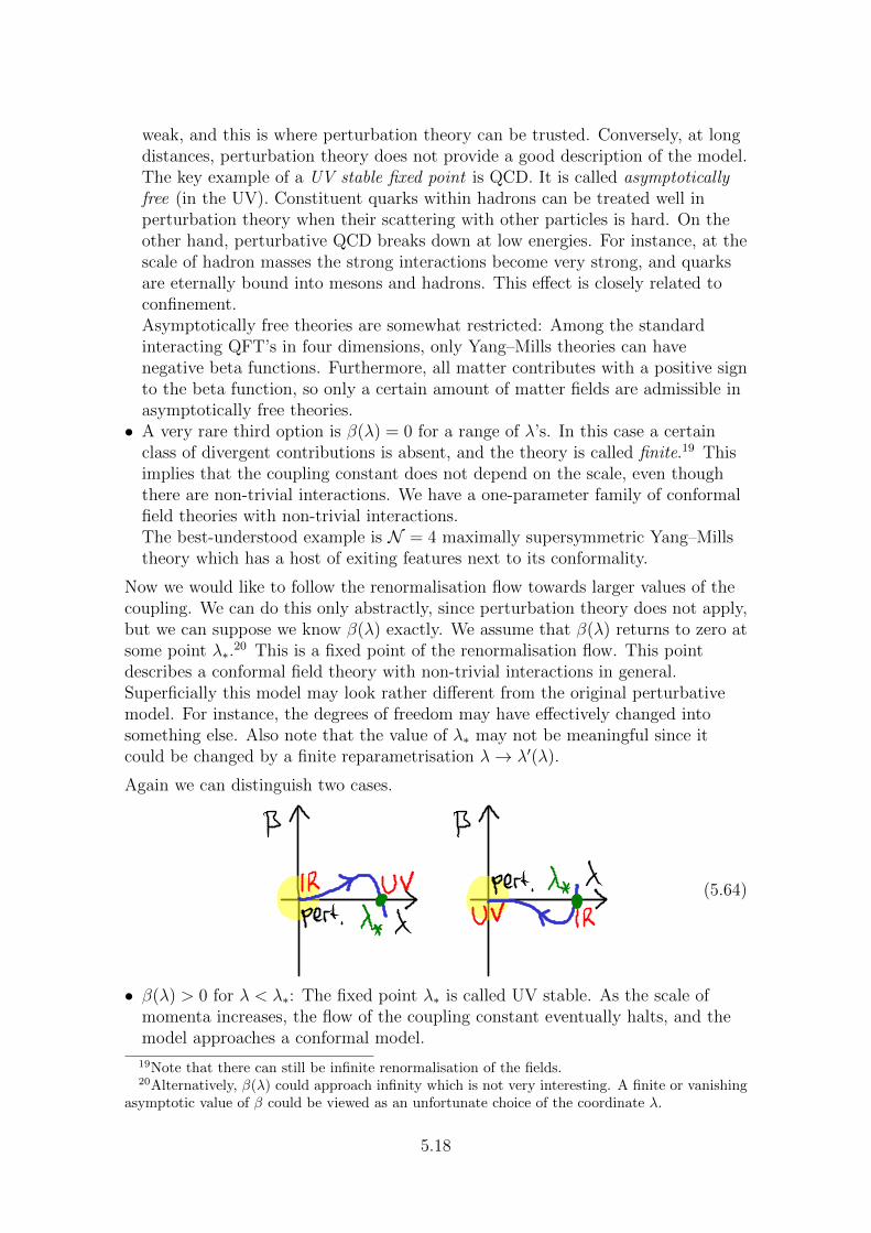
weak, and this is where perturbation theory can be trusted. Conversely, at longdistances, perturbation theory does not provide a good description of the model.The key example of a UV stable fixed point is QCD. It is called asymptoticallyfree (in the UV). Constituent quarks within hadrons can be treated well inperturbation theory when their scattering with other particles is hard. On theother hand, perturbative QCD breaks down at low energies. For instance, at thescale of hadron masses the strong interactions become very strong, and quarksare eternally bound into mesons and hadrons. This effect is closely related toconfinement.Asymptotically free theories are somewhat restricted: Among the standardinteracting QFT’s in four dimensions, only Yang–Mills theories can havenegative beta functions. Furthermore, all matter contributes with a positive signto the beta function, so only a certain amount of matter fields are admissible inasymptotically free theories.• A very rare third option is β(λ) = 0 for a range of λ’s. In this case a certain

class of divergent contributions is absent, and the theory is called finite.19 Thisimplies that the coupling constant does not depend on the scale, even thoughthere are non-trivial interactions. We have a one-parameter family of conformalfield theories with non-trivial interactions.The best-understood example is N = 4 maximally supersymmetric Yang–Millstheory which has a host of exiting features next to its conformality.

Now we would like to follow the renormalisation flow towards larger values of thecoupling. We can do this only abstractly, since perturbation theory does not apply,but we can suppose we know β(λ) exactly. We assume that β(λ) returns to zero atsome point λ∗.

20 This is a fixed point of the renormalisation flow. This pointdescribes a conformal field theory with non-trivial interactions in general.Superficially this model may look rather different from the original perturbativemodel. For instance, the degrees of freedom may have effectively changed intosomething else. Also note that the value of λ∗ may not be meaningful since itcould be changed by a finite reparametrisation λ→ λ′(λ).

Again we can distinguish two cases.

(5.64)

• β(λ) > 0 for λ < λ∗: The fixed point λ∗ is called UV stable. As the scale ofmomenta increases, the flow of the coupling constant eventually halts, and themodel approaches a conformal model.

19Note that there can still be infinite renormalisation of the fields.20Alternatively, β(λ) could approach infinity which is not very interesting. A finite or vanishing

asymptotic value of β could be viewed as an unfortunate choice of the coordinate λ.

5.18

• β(λ) < 0 for λ < λ∗: This fixed point λ∗ is called IR stable. As we go to largerdistances, we approach a conformal model.

In these cases, the renormalisation flow interpolates between two conformaltheories, one in the IR, the other in the UV. For correlation function this impliesscaling laws for short and for long distances. The scaling laws are different sincethe models are distinct CFT’s. One of them is a free field theory, the other one istypically a highly non-local field theory.

5.19

Quantum Field Theory II Chapter 6ETH Zurich, FS13 Prof. N. Beisert

11. 08. 2013

6 Quantum Symmetries

Symmetries are crucial for quantum field theories since they provide stability inthe renormalisation process. In particular, symmetries reduce the gauge field totwo polarisation modes.

Here we discuss the notion of symmetries at quantum level in the path integralframework. We derive a couple of identities which are analogues of Noether’stheorem for QFT.

6.1 Schwinger–Dyson Equations

Before we consider quantum symmetries, let us discuss the equation of motion atquantum level.

Equations of Motion. Quantum fields obey the equations of motion. In thepath integral they originate from an integrand which is a total derivative

0 =

∫DΨ

δ

δΨ(x)exp(iS[Ψ ] + iSsrc[Ψ, J ]

)= i

∫DΨ

(δS

δΨ(x)+ J(x)

)exp(iS[Ψ ] + iSsrc[Ψ, J ]

). (6.1)

The first term in the brackets generates the Euler–Lagrange equations, the secondone is usually removed by setting J = 0 in the end. In terms of the generatingfunctional this identity is known as the Schwinger–Dyson equation

δS

δΨ(x)

[−i δδJ

]Z[J ] = −J(x)Z[J ]. (6.2)

For example this implies the expectation value of the classical equation of motionto hold

〈δS[Ψ ]/δΨ(x)〉 = 0. (6.3)

In the presence of some other operator(s) O[Ψ ] in the correlator some more care isneeded because the functional derivatives in the operator can remove the source Jbefore it is set to zero

〈O[Ψ ] δS/δΨ(x)〉 = Z[J ]−1O

[−i δδJ

]δS

δΨ(x)

[−i δδJ

]Z[J ]

∣∣∣∣J=0

= − Z[J ]−1O

[−i δδJ

]J(x)Z[J ]

∣∣∣∣J=0

= iZ[J ]−1 δO

δΨ(x)

[−i δδJ

]Z[J ]

∣∣∣∣J=0

= i〈δO/δΨ(x)〉. (6.4)

6.1

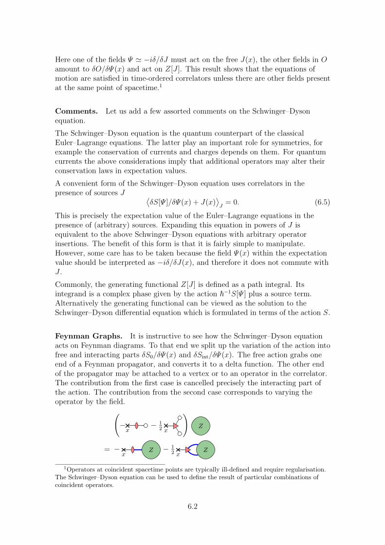
Here one of the fields Ψ ' −iδ/δJ must act on the free J(x), the other fields in Oamount to δO/δΨ(x) and act on Z[J ]. This result shows that the equations ofmotion are satisfied in time-ordered correlators unless there are other fields presentat the same point of spacetime.1

Comments. Let us add a few assorted comments on the Schwinger–Dysonequation.

The Schwinger–Dyson equation is the quantum counterpart of the classicalEuler–Lagrange equations. The latter play an important role for symmetries, forexample the conservation of currents and charges depends on them. For quantumcurrents the above considerations imply that additional operators may alter theirconservation laws in expectation values.

A convenient form of the Schwinger–Dyson equation uses correlators in thepresence of sources J ⟨

δS[Ψ ]/δΨ(x) + J(x)⟩J

= 0. (6.5)

This is precisely the expectation value of the Euler–Lagrange equations in thepresence of (arbitrary) sources. Expanding this equation in powers of J isequivalent to the above Schwinger–Dyson equations with arbitrary operatorinsertions. The benefit of this form is that it is fairly simple to manipulate.However, some care has to be taken because the field Ψ(x) within the expectationvalue should be interpreted as −iδ/δJ(x), and therefore it does not commute withJ .

Commonly, the generating functional Z[J ] is defined as a path integral. Itsintegrand is a complex phase given by the action ~−1S[Ψ ] plus a source term.Alternatively the generating functional can be viewed as the solution to theSchwinger–Dyson differential equation which is formulated in terms of the action S.

Feynman Graphs. It is instructive to see how the Schwinger–Dyson equationacts on Feynman diagrams. To that end we split up the variation of the action intofree and interacting parts δS0/δΨ(x) and δSint/δΨ(x). The free action grabs oneend of a Feynman propagator, and converts it to a delta function. The other endof the propagator may be attached to a vertex or to an operator in the correlator.The contribution from the first case is cancelled precisely the interacting part ofthe action. The contribution from the second case corresponds to varying theoperator by the field.(

−x

− 12 x

)Z

= − Zx

− 12 Zx

1Operators at coincident spacetime points are typically ill-defined and require regularisation.The Schwinger–Dyson equation can be used to define the result of particular combinations ofcoincident operators.

6.2

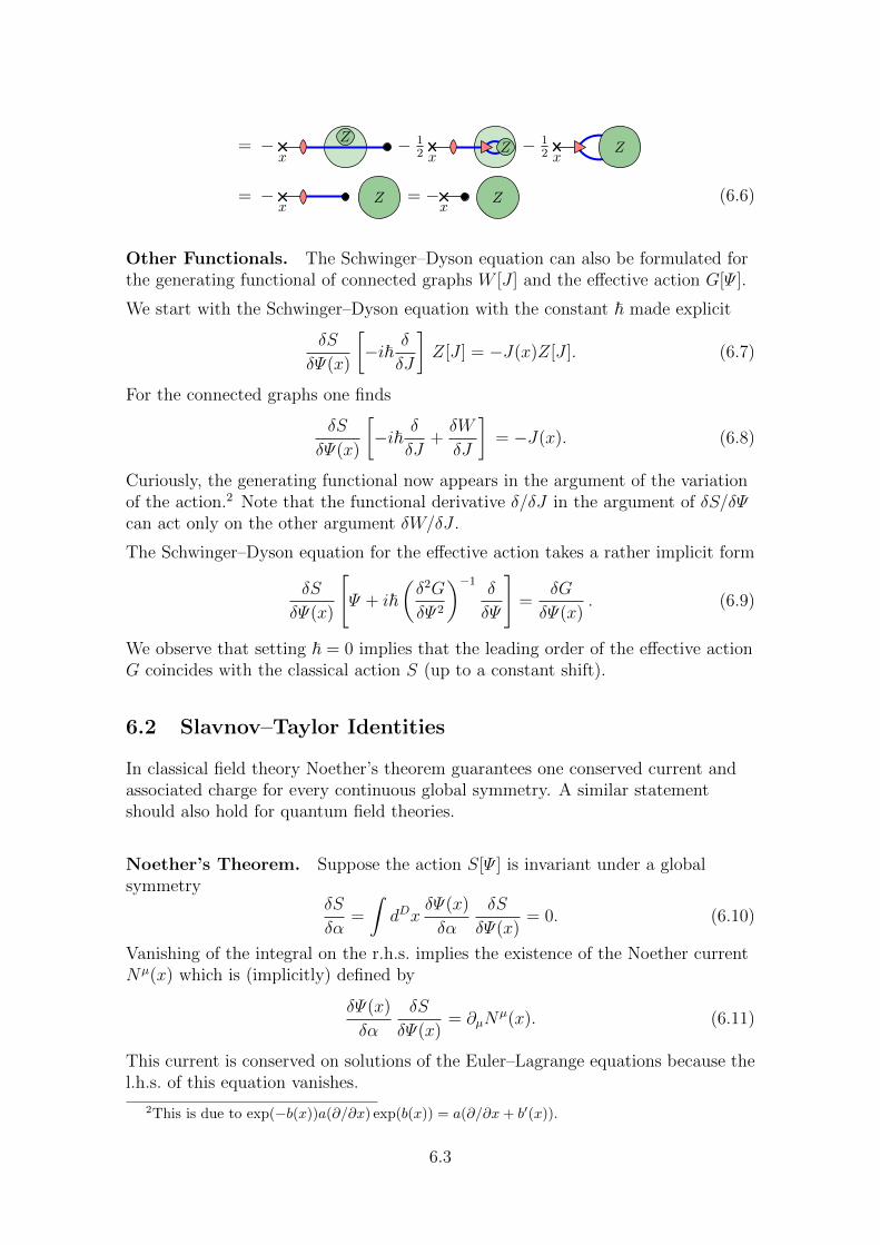
= − Z

x− 1

2 Zx

− 12 Zx

= −x

Z = −x

Z (6.6)

Other Functionals. The Schwinger–Dyson equation can also be formulated forthe generating functional of connected graphs W [J ] and the effective action G[Ψ ].

We start with the Schwinger–Dyson equation with the constant ~ made explicit

δS

δΨ(x)

[−i~ δ

δJ

]Z[J ] = −J(x)Z[J ]. (6.7)

For the connected graphs one finds

δS

δΨ(x)

[−i~ δ

δJ+δW

δJ

]= −J(x). (6.8)

Curiously, the generating functional now appears in the argument of the variationof the action.2 Note that the functional derivative δ/δJ in the argument of δS/δΨcan act only on the other argument δW/δJ .

The Schwinger–Dyson equation for the effective action takes a rather implicit form

δS

δΨ(x)

[Ψ + i~

(δ2G

δΨ 2

)−1δ

δΨ

]=

δG

δΨ(x). (6.9)

We observe that setting ~ = 0 implies that the leading order of the effective actionG coincides with the classical action S (up to a constant shift).

6.2 Slavnov–Taylor Identities

In classical field theory Noether’s theorem guarantees one conserved current andassociated charge for every continuous global symmetry. A similar statementshould also hold for quantum field theories.

Noether’s Theorem. Suppose the action S[Ψ ] is invariant under a globalsymmetry

δS

δα=

∫dDx

δΨ(x)

δα

δS

δΨ(x)= 0. (6.10)

Vanishing of the integral on the r.h.s. implies the existence of the Noether currentNµ(x) which is (implicitly) defined by

δΨ(x)

δα

δS

δΨ(x)= ∂µN

µ(x). (6.11)

This current is conserved on solutions of the Euler–Lagrange equations because thel.h.s. of this equation vanishes.

2This is due to exp(−b(x))a(∂/∂x) exp(b(x)) = a(∂/∂x+ b′(x)).

6.3

Generating Functional. We have already derived the quantum analog of theEuler–Lagrange equation, namely the Schwinger–Dyson equation3

δS

δΨ(x)

[−i δδJ

]Z[J ] = −J(x)Z[J ]. (6.12)

Multiplying this identity by the field variation we find(δΨ(x)

δα

δS

δΨ(x)

)[−i δδJ

]Z[J ] = −δΨ(x)

δα

[−i δδJ

]J(x)Z[J ]. (6.13)

We substitute the Noether current to obtain the Slavnov–Taylor equation

∂µNµ

[−i δδJ

](x)Z[J ] = −δΨ(x)

δα

[−i δδJ

] (J(x)Z[J ]

). (6.14)

In the integral form the Noether current drops out∫dDx

δΨ(x)

δα

[−i δδJ

] (J(x)Z[J ]

)= 0. (6.15)

The content of the above statements is clearer when expanded in powers of J .Their expansion coefficients are identities between quantum correlation functions.For instance, the leading order of the differential form is the classical conservationlaw of the expectation value ⟨

∂·N(x)⟩

= 0. (6.16)

The term at first order yields in differential form reads⟨Ψ(y) ∂µN

µ(x)⟩

= iδD(x− y)⟨δΨ(x)/δα

⟩. (6.17)

Here, the current is conserved unless there is another field at coincident location.Note that the extra term equals the symmetry variation of the other field.Therefore, one can view the current divergence ∂·N(x) to be a symmetry generatorlocalised at x.4

After integration over x we find the global field variation⟨δΨ(y)/δα

⟩= 0. (6.18)

In words it tells us that the expectation value of the change of Ψ vanishes. This isobvious since the transformed field Ψ ′ is related to Ψ by symmetry.

The same holds at second order⟨(δΨ(y)/δα)Ψ(z)

⟩+⟨Ψ(y)(δΨ(z)/δα)

⟩= 0 (6.19)

telling that the expectation value of the change of the product Ψ(y)Ψ(z) vanishes.

3Recall that a functional F [−iδ/δJ ] acting on Z[J ] should be interpreted as the functionalF [Ψ ] within a quantum correlator 〈. . .〉J .

4This is somewhat analogous to the Noether charge acting as a symmetry generator in thecanonical framework.

6.4

Correlators with Sources. Altogether these relationships are no big surprises.In fact it makes sense to write the Slavnov–Taylor equation in terms of a correlatorin the presence of sources⟨

∂µNµ(x) + J(x) (δΨ(x)/δα)

⟩J

= 0. (6.20)

The argument of the correlator is just the classical conservation of the Noethercurrent when sources are included. The pleasant feature of this equation is thatadditional fields can be introduced into the correlator by means of the sources.

Example. Consider the interacting complex scalar field with Lagrangian

L = −∂µφ∗∂µφ−m2φ∗φ− 14λ(φ∗φ)2. (6.21)

Rotation of the fields by a phase δφ = iδα φ, δφ∗ = −iδα φ∗ is a continuous globalsymmetry. We define the associated Noether current via

iφ ∂2φ∗ − iφ∗∂2φ = ∂µNµ ⇒ Nµ = iφ ∂µφ∗ − iφ∗∂µφ. (6.22)

We can now write the above Slavnov–Taylor equation in terms of a correlator withsources ⟨

∂µNµ(x)

⟩j,j∗

= −i⟨φ(x)j(x)− φ∗(x)j∗(x)

⟩j,j∗. (6.23)

Disabling the sources leads to the classical conservation law for the expectationvalue ⟨

∂µNµ(x)

⟩= 0. (6.24)

However, the conservation law is deformed when additional fields are inserted intothe correlator via φ = −iδ/δj⟨

∂µNµ(x)φ(y)

⟩= −δD(x− y)

⟨φ(y)

⟩. (6.25)

Integration over x yields the statement that the expectation value of a chargedquantity vanishes ⟨

φ(y)⟩

= 0. (6.26)

For insertion of two fields we find

〈∂µNµ(x)φ(y)φ∗(z)〉 = −(δD(x− y)− δD(x− z))〈φ(y)φ∗(z)〉. (6.27)

Note that this identity holds exactly even in the presence of interactions. Here theintegration over x yields a trivial statement. In other words, the symmetry permitsa non-trivial expectation value of the uncharged correlator

⟨φ(y)φ∗(z)

⟩.

6.3 Ward–Takahashi Identity

QED is a gauge theory with one abelian gauge symmetry. In the quantisationprocess we have broken Gauge invariance, but a global U(1) invariance remains.The Slavnov–Taylor identity for the latter is called Ward–Takahashi identity. Itguarantees consistent renormalisation of the coupling constant (charges).

6.5

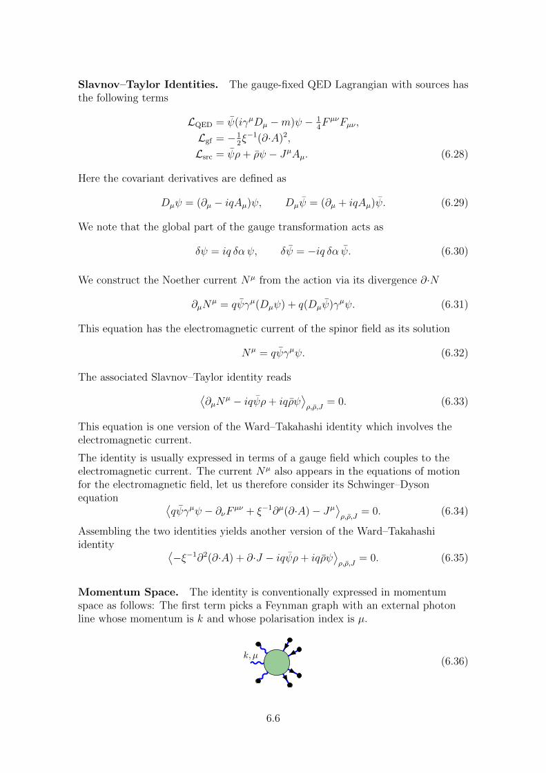
Slavnov–Taylor Identities. The gauge-fixed QED Lagrangian with sources hasthe following terms

LQED = ψ(iγµDµ −m)ψ − 14F µνFµν ,

Lgf = −12ξ−1(∂·A)2,

Lsrc = ψρ+ ρψ − JµAµ. (6.28)

Here the covariant derivatives are defined as

Dµψ = (∂µ − iqAµ)ψ, Dµψ = (∂µ + iqAµ)ψ. (6.29)

We note that the global part of the gauge transformation acts as

δψ = iq δα ψ, δψ = −iq δα ψ. (6.30)

We construct the Noether current Nµ from the action via its divergence ∂·N

∂µNµ = qψγµ(Dµψ) + q(Dµψ)γµψ. (6.31)

This equation has the electromagnetic current of the spinor field as its solution

Nµ = qψγµψ. (6.32)

The associated Slavnov–Taylor identity reads⟨∂µN

µ − iqψρ+ iqρψ⟩ρ,ρ,J

= 0. (6.33)

This equation is one version of the Ward–Takahashi identity which involves theelectromagnetic current.

The identity is usually expressed in terms of a gauge field which couples to theelectromagnetic current. The current Nµ also appears in the equations of motionfor the electromagnetic field, let us therefore consider its Schwinger–Dysonequation ⟨

qψγµψ − ∂νF µν + ξ−1∂µ(∂·A)− Jµ⟩ρ,ρ,J

= 0. (6.34)

Assembling the two identities yields another version of the Ward–Takahashiidentity ⟨

−ξ−1∂2(∂·A) + ∂·J − iqψρ+ iqρψ⟩ρ,ρ,J

= 0. (6.35)

Momentum Space. The identity is conventionally expressed in momentumspace as follows: The first term picks a Feynman graph with an external photonline whose momentum is k and whose polarisation index is µ.

k, µ(6.36)

6.6

It multiplies the graph by ξ−1k2kµ. The external photon line connects to theremainder of the graph by the propagator

GµνF (k) =

ηµν − (1− ξ)kµkν/k2

k2 − iε. (6.37)

Multiplied by the prefactor we obtain

ξ−1k2kµGµνF (k) = kν . (6.38)

This means we actually consider a graph with one amputated photon line whosepolarisation vector is contracted with k. Now there are two options:

k, µ

k, µ(6.39)

• The other side of the photon propagator is connected to a source J , i.e. weconsider a plain photon propagator (disconnected from the remainder of thegraph). In this case we obtain ∂·J which cancels precisely the correspondingterm in the Ward–Takahashi identity. This part of the identity is somewhattrivial as it concerns only a plain photon propagator.• Otherwise, the photon line connects to a non-trivial (sub)graph. The remaining

two terms involving spinors and sources must cancel this graph. They pick aspinor line of a graph with one fewer photon line. They shift the spinormomentum by k, and they multiply the graph by the charge ±q of the particle.The sum over all external spinor lines should then precisely cancel the sum overall photon insertions as explained above.

kµ∑

photon

k, µ=∑

matter

(±q)

p+ k

(6.40)

Propagator and Vertex. Let us consider two examples, a photon propagatorand a spinor-photon vertex:

We have already seen that the plain photon propagator GµνF (k) satisfies the

identity, and it absorbs the term ∂·J completely. How about the loop correctionMµν(k)? Consider the graph ξ−1k2kµM

µν(k) with one external photon lineamputated and contracted with its own momentum. As there are no externalspinor lines, this graph must vanish exactly. We learn that the loop corrections tothe propagator must be exactly transversal

Mµν(k) ∼ ηµν − kµkν/k2. (6.41)

The only violation of transversality originates from the gauge fixing term in theplain propagator. This identity our earlier claim in the context of introduction ofghost fields.

6.7

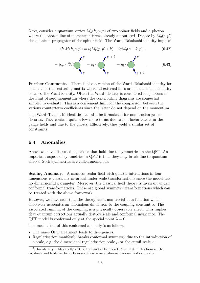
Next, consider a quantum vertex Mµ(k, p, p′) of two spinor fields and a photonwhere the photon line of momentum k was already amputated. Denote by M0(p, p′)the quantum propagator of the spinor field. The Ward–Takahashi identity implies5

− ik·M(k, p, p′) = iqM0(p, p′ + k)− iqM0(p+ k, p′). (6.42)

− ikµ · k, µ

p

p′

= iq ·

p

p′ + k

− iq ·

p+ k

p′

. (6.43)

Further Comments. There is also a version of the Ward–Takahashi identity forelements of the scattering matrix where all external lines are on-shell. This identityis called the Ward identity. Often the Ward identity is considered for photons inthe limit of zero momentum where the contributing diagrams are somewhatsimpler to evaluate. This is a convenient limit for the comparison between thevarious counterterm coefficients since the latter do not depend on the momentum.

The Ward–Takahashi identities can also be formulated for non-abelian gaugetheories. They contain quite a few more terms due to non-linear effects in thegauge fields and due to the ghosts. Effectively, they yield a similar set ofconstraints.

6.4 Anomalies

Above we have discussed equations that hold due to symmetries in the QFT. Animportant aspect of symmetries in QFT is that they may break due to quantumeffects. Such symmetries are called anomalous.

Scaling Anomaly. A massless scalar field with quartic interactions in fourdimensions is classically invariant under scale transformations since the model hasno dimensionful parameter. Moreover, the classical field theory is invariant underconformal transformations. These are global symmetry transformations which canbe treated with the above framework.

However, we have seen that the theory has a non-trivial beta function whicheffectively associates an anomalous dimension to the coupling constant λ. Theassociated running of the coupling is a physically observable effect. This impliesthat quantum corrections actually destroy scale and conformal invariance. TheQFT model is conformal only at the special point λ = 0.

The mechanism of this conformal anomaly is as follows:

• The naive QFT treatment leads to divergences.• Regularisation manifestly breaks conformal symmetry due to the introduction of

a scale, e.g. the dimensional regularisation scale µ or the cutoff scale Λ.

5This identity holds exactly at tree level and at loop level. Note that in this form all theconstants and fields are bare. However, there is an analogous renormalised expression.

6.8

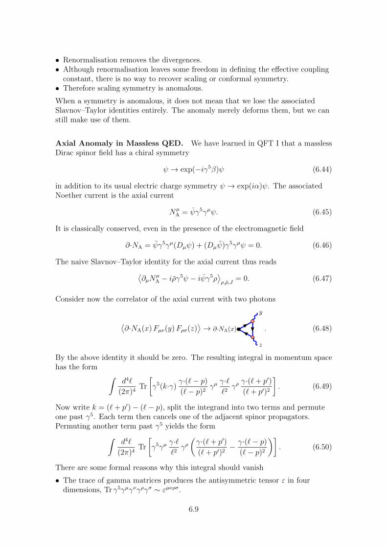
• Renormalisation removes the divergences.• Although renormalisation leaves some freedom in defining the effective coupling

constant, there is no way to recover scaling or conformal symmetry.• Therefore scaling symmetry is anomalous.

When a symmetry is anomalous, it does not mean that we lose the associatedSlavnov–Taylor identities entirely. The anomaly merely deforms them, but we canstill make use of them.

Axial Anomaly in Massless QED. We have learned in QFT I that a masslessDirac spinor field has a chiral symmetry

ψ → exp(−iγ5β)ψ (6.44)

in addition to its usual electric charge symmetry ψ → exp(iα)ψ. The associatedNoether current is the axial current

NµA = ψγ5γµψ. (6.45)

It is classically conserved, even in the presence of the electromagnetic field

∂·NA = ψγ5γµ(Dµψ) + (Dµψ)γ5γµψ = 0. (6.46)

The naive Slavnov–Taylor identity for the axial current thus reads⟨∂µN

µA − iργ

5ψ − iψγ5ρ⟩ρ,ρ,J

= 0. (6.47)

Consider now the correlator of the axial current with two photons

⟨∂·NA(x)Fµν(y)Fρσ(z)

⟩→ ∂·NA(x)

y

z

. (6.48)

By the above identity it should be zero. The resulting integral in momentum spacehas the form ∫

d4`

(2π)4Tr

[γ5(k·γ)

γ·(`− p)(`− p)2

γµγ·``2

γργ·(`+ p′)

(`+ p′)2

]. (6.49)

Now write k = (`+ p′)− (`− p), split the integrand into two terms and permuteone past γ5. Each term then cancels one of the adjacent spinor propagators.Permuting another term past γ5 yields the form∫

d4`

(2π)4Tr

[γ5γµ

γ·``2

γρ(γ·(`+ p′)

(`+ p′)2− γ·(`− p)

(`− p)2

)]. (6.50)

There are some formal reasons why this integral should vanish

• The trace of gamma matrices produces the antisymmetric tensor ε in fourdimensions, Tr γ5γµγνγργσ ∼ εµνρσ.

6.9

• The two resulting integrals should depend on either p or p′ but not on both.• Altogether there are only three vectors or indices at our disposal: µ, ρ and p orp′. There is nothing to act as the fourth index of ε.• Furthermore, there is another copy of the same integral with the photon lines

exchanged. This appears to cancel against the above integral due to statistics.

This conclusion is however too naive: One must pay attention to the fact that theabove integral is divergent. Subtracting two divergent integrals is an ambiguousoperation. The result may in principle be adjusted to any desired value, be it zero,finite or infinite. Nevertheless, the result for the overall integral is finite and ityields a well-defined, non-zero quantity proportional to εµνρσpρp

′σ.

The pitfall in the above considerations depends on the regularisation scheme:

• In a cutoff regularisation scheme, one has to pay attention to the boundary ofthe integration region. In particular, the evaluation of integrals involves a shift.Since the original integral is linearly divergent, such a shift may well result in afinite difference.• In dimensional regularisation the mistake was to assume that γ5 anti-commutes

with all γµ. First of all γ5 is a strictly 4-dimensional concept. One can still definean antisymmetric product of 4 gamma matrices which imitates the behaviour ofγ5. However, there are discrepancies at O(ε). For instance, it anticommuteswith 4 gamma matrices but it commutes with the remaining (−2ε) ones.

γ5γµ 6= −γµγ5. (6.51)

The resulting factor of ε is then cancelled by a factor of 1/ε from a divergentloop integral.

Curiously, a careful evaluation in either of the two schemes yields the same result.It can be summarised in the anomalous Slavnov–Taylor identity known as theAdler–Bell–Jackiw identity⟨

∂µAµ − iργ5ψ − iψγ5ρ− q2(4π)−2 εµνρσFµνFρσ

⟩ρ,ρ,J

= 0. (6.52)

Note that the additional term has the expected structure εµνρσpρp′σ which is

perfectly local. Adler and Bardeen showed that this identity is exact, there are nofurther corrections from higher loop orders.

Comments. Anomalies are an exciting topic of quantum field theory related totopological issues of spacetime and gauge groups. It is treated in more detail in thecourse on advanced field theory. Let us nevertheless make a few more remarks:

Gauge fields can also be coupled to the axial current. In fact, the electroweaksector of the standard model relies on such couplings. The presence of an axialanomaly would be disastrous since it would violate gauge invariance. Gladly, allsuch anomalies cancel in the standard model due to a particular arrangement ofspinor fields. This is called anomaly cancellation and it represents one of theconsistency requirements of QFT on the particle spectrum.

Note that the coupling of a chiral spinor to a gauge field effectively is acombination of vector and axial vector currents. Hence, chiral spinor fields are the

6.10

origin of the so-called chiral anomaly. The chiral anomaly for quarks can beobserved in meson decay.

Anomalies are universal statements of QFT. They state that certain symmetriesare incompatible with the quantisation procedure. An anomaly can only occur fornon-manifest symmetries which are not respected by the regulator. When theregulator is removed after renormalisation, some of these non-manifest symmetriesmay turn out intact if the renormalisation parameters are chosen appropriately. Ifthere is no way to recover the symmetry using local counterterms, the symmetry isanomalous.

The amount by which the symmetry is broken is a universal statementindependent of the regularisation scheme. An anomalous Slavnov–Taylor identityis often one-loop exact.

Note that even though anomalies are universal, some details may depend on theimplementation. Some anomalies refer to pairs of symmetries which cannot berealised simultaneously. The renormalisation process can be adjusted to preserveone symmetry at the cost of the other. Alternatively the other symmetry can bepreserved with suitable counterterms. A third option is to break both symmetries.For example, the axial current can be made to be exactly conserved, but only atthe cost of an anomaly for the vector current. The latter is highly undesirablesince it would definitely break gauge invariance. Therefore, one usually makes surethat the vector current is non-anomalous.

6.11

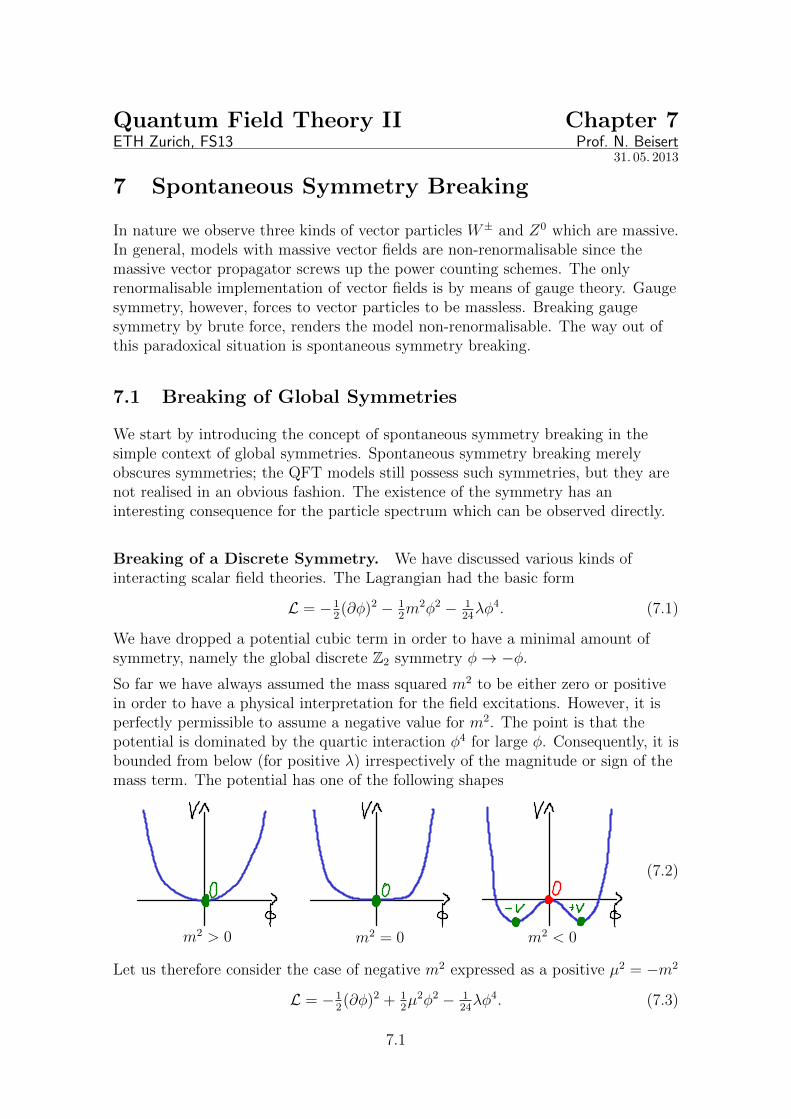
Quantum Field Theory II Chapter 7ETH Zurich, FS13 Prof. N. Beisert

31. 05. 2013

7 Spontaneous Symmetry Breaking

In nature we observe three kinds of vector particles W± and Z0 which are massive.In general, models with massive vector fields are non-renormalisable since themassive vector propagator screws up the power counting schemes. The onlyrenormalisable implementation of vector fields is by means of gauge theory. Gaugesymmetry, however, forces to vector particles to be massless. Breaking gaugesymmetry by brute force, renders the model non-renormalisable. The way out ofthis paradoxical situation is spontaneous symmetry breaking.

7.1 Breaking of Global Symmetries

We start by introducing the concept of spontaneous symmetry breaking in thesimple context of global symmetries. Spontaneous symmetry breaking merelyobscures symmetries; the QFT models still possess such symmetries, but they arenot realised in an obvious fashion. The existence of the symmetry has aninteresting consequence for the particle spectrum which can be observed directly.

Breaking of a Discrete Symmetry. We have discussed various kinds ofinteracting scalar field theories. The Lagrangian had the basic form

L = −12(∂φ)2 − 1

2m2φ2 − 1

24λφ4. (7.1)

We have dropped a potential cubic term in order to have a minimal amount ofsymmetry, namely the global discrete Z2 symmetry φ→ −φ.

So far we have always assumed the mass squared m2 to be either zero or positivein order to have a physical interpretation for the field excitations. However, it isperfectly permissible to assume a negative value for m2. The point is that thepotential is dominated by the quartic interaction φ4 for large φ. Consequently, it isbounded from below (for positive λ) irrespectively of the magnitude or sign of themass term. The potential has one of the following shapes

m2 > 0 m2 = 0 m2 < 0

(7.2)

Let us therefore consider the case of negative m2 expressed as a positive µ2 = −m2

L = −12(∂φ)2 + 1

2µ2φ2 − 1

24λφ4. (7.3)

7.1

Evidently, the expansion of the field around a classical value φ = 0 leads toundesirable tachyonic excitations. In other words, φ = 0 is a stationary point ofthe potential; it is however not a local minimum, but rather a local maximum.1

Since the potential is bounded from below, the must be a minimum somewherearound which we can quantise the model. In fact, there are two local minima at

φ = ±v, v =√

6µ2/λ . (7.4)

The constant field φ(x) = ±v is a solution to the equation of motion. We cantherefore expand the field φ around this solution

φ(x) = ±v + η(x), (7.5)

where η serves as the quantum field. The expectation value of the quantum field inthe vacuum is defined to be zero, hence v is the vacuum expectation value of φ(x)

〈φ(x)〉 = ±v. (7.6)

We obtain a new Lagrangian in the new field η

L = −12(∂η)2 + 3µ4/2λ− µ2η2 ∓

√λµ2/6 η3 − 1

24λη4. (7.7)

This is again a Lagrangian in the same class of scalar field theories. Let us discussthe terms that arise:

• The derivative term and the quartic interactions have not changed.• The constant term does not actually play a role, we can disregard it.• The term linear in η receives two contributions which cancel exactly. This is the

condition of the minimum.• We obtain a regular mass term with mass m =

√2µ.

• There is a new cubic term with coefficient fixed by the quartic coupling andmass term.

The cubic term evidently violates the Z2 symmetry η → −η, but altogether theoriginal symmetry is still present in the somewhat obscure form

η → ∓2v − η. (7.8)

This symmetry survives quantisation, but it is not compatible with the vacuumexpectation value of the fields. The symmetry is said to be spontaneously broken.

The model has two possible ground state configurations φ = ±v, Both are globalminima of the potential. Which one should we choose as the ground state? Thereis no criterion to prefer one state over the other. This is the generic situation forspontaneous symmetry breaking: Since symmetry does not leave the ground stateinvariant, it must map it to some other state. This state has equivalent properties

1In fact, a local maximum is troublesome only due to perturbation theory. When we turn offthe interactions, the potential all of a sudden becomes unbounded from below. In other words,perturbation theory tries to expand around a tachyonic model. If somehow the interacting theorycould be treated non-perturbatively, the expansion point φ = 0 could be suitable as well.

7.2

and therefore is also a ground state. Hence, spontaneous symmetry breakingimplies degeneracy of the ground state. Which one of the two we choose makes nodifference since all physics is the same for both states.2 We can thus setφ(x) = +v + η(x) without prejudice.3

Breaking of a Continuous Symmetry. Next, consider a generalisation of theabove model to N scalar fields Φa with a global O(N) symmetry

L = −12(∂Φ)2 + 1

2µ2Φ2 − 1

8λ(Φ2)2. (7.9)

The potential has a local maximum at Φ = 0, and a family of global minima at thespherical surface defined by

Φ2 = v2, v =√

2µ2/λ . (7.10)

As discussed above, all of these points are related by O(N) symmetry and aretherefore equivalent. Without prejudice we can choose any representative, e.g.

Φ0 = (0, . . . , 0, v). (7.11)

We thus introduce the quantum fields η and φa with a = 1, . . . , N − 1

Φa(x) =

φa(x) for a = 1, . . . , N − 1,

v + η(x) for a = N.(7.12)

Substitution in the Lagrangian yields the terms

L = − 12(∂φ)2 − 1

8λ(φ2)2

− 12(∂η)2 − µ2η2 −

√λµ2/2 η3 − 1

8λη4

+ µ4/2λ−√λµ2/2φ2η − 1

4λφ2η2. (7.13)

It describes a scalar field with mass m =√

2µ and N − 1 massless scalar fieldswhich interact in a particular pattern. It has a manifest O(N − 1) symmetry of thescalars φa which enlarges to the original O(N) symmetry in a non-evident fashion.

The fact that there are N − 1 massless fields is remarkable. It is a consequence ofGoldstone’s theorem.

Goldstone’s Theorem. Goldstone’s theorem asserts that for everyspontaneously broken continuous global symmetry there is one massless particlewith the same quantum numbers. For ordinary symmetries the particle is a scalar,called the Goldstone boson.

One can understand the statement at the level of the Lagrangian of a model ofscalar fields Φa:

2One could also consider linear combinations of ground states. In our situation, however, themixing is strongly discouraged because transitions between the ground states have infinite energy.

3Fixing one of the ground states may appear paradoxical in the path integral framework: Itsums over all field configurations which appears to include all ground states, so how can wespecialise to one? In fact we should specify some boundary conditions for the fields. The vacuumexpectation value is thus implemented as the field value in asymptotic regions of spacetime.

7.3

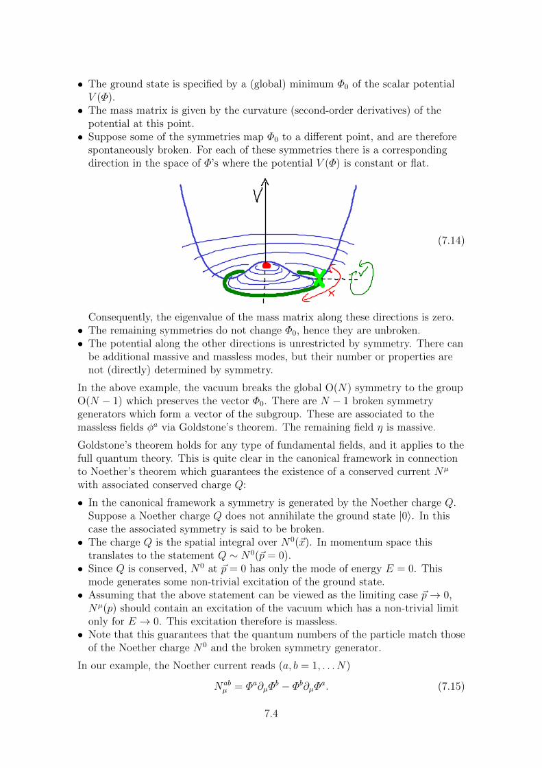
• The ground state is specified by a (global) minimum Φ0 of the scalar potentialV (Φ).• The mass matrix is given by the curvature (second-order derivatives) of the

potential at this point.• Suppose some of the symmetries map Φ0 to a different point, and are therefore

spontaneously broken. For each of these symmetries there is a correspondingdirection in the space of Φ’s where the potential V (Φ) is constant or flat.

(7.14)

Consequently, the eigenvalue of the mass matrix along these directions is zero.• The remaining symmetries do not change Φ0, hence they are unbroken.• The potential along the other directions is unrestricted by symmetry. There can

be additional massive and massless modes, but their number or properties arenot (directly) determined by symmetry.

In the above example, the vacuum breaks the global O(N) symmetry to the groupO(N − 1) which preserves the vector Φ0. There are N − 1 broken symmetrygenerators which form a vector of the subgroup. These are associated to themassless fields φa via Goldstone’s theorem. The remaining field η is massive.

Goldstone’s theorem holds for any type of fundamental fields, and it applies to thefull quantum theory. This is quite clear in the canonical framework in connectionto Noether’s theorem which guarantees the existence of a conserved current Nµ

with associated conserved charge Q:

• In the canonical framework a symmetry is generated by the Noether charge Q.Suppose a Noether charge Q does not annihilate the ground state |0〉. In thiscase the associated symmetry is said to be broken.• The charge Q is the spatial integral over N0(~x). In momentum space this

translates to the statement Q ∼ N0(~p = 0).• Since Q is conserved, N0 at ~p = 0 has only the mode of energy E = 0. This

mode generates some non-trivial excitation of the ground state.• Assuming that the above statement can be viewed as the limiting case ~p→ 0,Nµ(p) should contain an excitation of the vacuum which has a non-trivial limitonly for E → 0. This excitation therefore is massless.• Note that this guarantees that the quantum numbers of the particle match those

of the Noether charge N0 and the broken symmetry generator.

In our example, the Noether current reads (a, b = 1, . . . N)

Nabµ = Φa∂µΦ

b − Φb∂µΦa. (7.15)

7.4

Expressed in terms of the new fields we find (a, b = 1, . . . N − 1)

Nabµ = φa∂µφ

b − φb∂µφa, NNaµ = v∂µφ

a + η∂µφa − φa∂µη. (7.16)

We note that for the latter N − 1 currents, there is a contribution linear in thefields. These currents NNa

µ indeed create (and annihilate) the massless particles φa

from the ground state |0〉. Conversely, the unbroken currents Nabµ are quadratic in

the fields and always consist of one creation and one annihilation operator, so theypreserve the particle number.

There are also situations where Noether’s theorem is less obvious. For example, inQCD it can be used to argue for the lightest pseudoscalar mesons. QCD is atheory of spinor and gauge fields. It is strongly coupled at the nuclear scale whichis substantially higher than the fundamental quark masses. At nuclear scales, itmakes sense to approximate the quark masses by zero. Then the quark fields havean (approximate) axial symmetry. Suppose the axial symmetry is spontaneouslybroken (by a scalar expectation value of quark bilinears). This would lead to theexistence of massless pseudoscalar mesons. However, since axial symmetry is notexact in the presence of fermion masses, one would expect the pseudoscalar mesonsto have a reasonably small mass as well. This is the case for the pions which onecould consider as the pseudo-Goldstone bosons of a spontaneously and explicitlybroken axial SU(2) flavour symmetry relating the up and down quarks.

7.2 Breaking of Gauge Symmetries

The picture changes again when the spontaneously broken symmetry belong to alocal symmetry. The coupling of currents to gauge fields leads to massive vectorfields instead of Goldstone bosons.

Higgs Mechanism. The above model for N = 2 is equivalent to a complexscalar field φ, φ∗ We couple it to the electromagnetic field to obtain scalar QED,but we assume that the mass term has the opposite sign

LSQED = −(Dµφ)∗(Dµφ) + µ2φ∗φ− 14λ(φ∗φ)2 − 1

4F µνFµν . (7.17)

The covariant derivative is defined as Dµφ = ∂µφ− iqAµφ.

Here the ground state solution is specified by a point on a circle in the complexplane

φ∗φ = 12v2, v =

√4µ2/λ, (7.18)

We could go ahead as before and introduce a shifted quantum field

φ(x) =1√2

(v + η(x) + iρ(x)

). (7.19)

This would lead to the same form of Lagrangian as above with the exception of thekinetic term which yields

−(Dµφ)∗(Dµφ) = − 12(∂η)2 − 1

2(∂ρ)2 − 1

2q2v2A2 + qvAµ∂

µρ

+ interactions. (7.20)

7.5

As it stands this is not a very pleasant form due to the quadratic coupling betweenthe gauge field Aµ and the scalar field ρ. We must first diagonalise by shifting thegauge field appropriately

Aµ(x) = Vµ(x) + (qv)−1∂µρ(x). (7.21)

This shift changes the kinetic terms in the Lagrangian substantially

− (Dµφ)∗(Dµφ) = −12(∂η)2 − 1

2q2v2V 2 + interactions. (7.22)

Note that the kinetic term for the field ρ has cancelled out exactly. What remainsis one scalar field η and a mass term for the vector field with mass m = qv.

This is the Higgs effect:4 The coupling of the gauge field to a conserved current ofa spontaneously broken symmetry lends the gauge field a mass. Moreover, one ofthe scalar fields is absorbed completely by this process.

There is an alternative parametrisation of the fields which makes the abovestatement more obvious. The crucial observation is that the abovereparametrisation of the gauge field is a gauge transformation. We thus split thecomplex scalar field into absolute value and complex phase

φ(x) =1√2

(v + η(x)

)exp(iα(x)

). (7.23)

By means of a gauge transformation we can remove the phase from the field φwithout changing any of the terms in the Lagrangian

φ(x) =1√2

(v + η(x)

). (7.24)

It appears as though one degree of freedom is lost. However, it is compensated bythe loss of gauge symmetry since the field φ is now real and must not be rotated inthe complex plane. Gauge symmetry effectively removes one degree of freedomfrom the gauge field. In that sense, we have merely transferred the complex phaseof φ into the field Aµ which henceforth should be considered a vector field Vµrather than a gauge field. The resulting Lagrangian reads

LSQED = − 12(∂η)2 − 1

4v2λη2

− 12(∂µV ν)(∂µVν) + 1

2(∂·V )2 − 1

2q2v2V 2

+ 116v4λ− 1

4λvη3 − 1

16λη4 − q2vV 2η − 1

2q2V 2η2. (7.25)

We thus obtain a scalar field η with mass√v2λ/2 and a vector field Vµ with mass

qv. The scalar field interacts with itself and with the square of the vector field.

The Lagrangian has a very special form: Altogether it has 2 mass terms and 5interaction terms (the coefficient of ηVµ∂

µη is zero). Using the Z2 symmetryη → −2v − η these numbers reduce to 4 coefficients. However, there are only threeparameters v, q and λ, so there is one constraint among the set of conceivableparameters. This feature is owed to the gauge symmetry in the originalformulation of the Lagrangian. It will be crucial for a successful renormalisation.

4In October 2013 we will learn which names of the set Anderson, Brout, Englert, Guralnik,Hagen, Higgs, Kibble and ’t Hooft we should “officially” associate to the effect.

7.6

Comments. Above we have presented an example of the Higgs mechanism foran abelian gauge symmetry. The Higgs mechanism works analogously for anon-abelian gauge symmetry: For each broken generator of the gauge group, theassociated gauge field acquires a mass. Goldstone bosons never appear for brokengauge symmetries.

The configuration of massive scalar fields very much depends on the particularmodel. In principle, spontaneous symmetry breaking can be achieved withoutadditional massive scalar fields. For example, sigma models on group manifoldsand coset spaces thereof are particular implementations. However, these modelstypically have non-polynomial interactions and therefore are non-renormalisable.Spontaneous symmetry breaking in models with polynomial interactions requiresthe presence of at least one massive scalar field.5 In that sense, the Higgsmechanism implies a massive scalar field, the so-called Higgs particle.

Note that the number of independent particle modes is preserved by the Higgsmechanism: We start with some scalar fields and some massless vector fields. Foreach broken generator of the gauge algebra one of the scalar fields disappears infavour of a massive vector field. A massless vector field has two on-shell degrees offreedom whereas a massive one has three. The additional degree of freedomoriginates from the scalar field; the gauge field eats a scalar field to becomemassive.6

Renormalisation. We could now proceed and quantise the above Lagrangian.The model includes a massive vector field whose propagator is

Gµν(p) =ηµν + pµpν/m2

p2 +m2. (7.26)

The trouble with this massive vector field propagator is that for large momenta pit approaches a finite value rather than decaying quadratically. This makes the UVbehaviour far worse than for an ordinary gauge field. Moreover, the appearance ofthe inverse of the mass spoils power counting. This generically renders the modelnon-renormalisable.

Now the above Lagrangian is very special, and the UV divergences in fact cancelsuch that the model remains renormalisable. This nice behaviour evidently is dueto gauge symmetry in the original model: One could argue that the model withspontaneous symmetry breaking is really just the same as the model where gaugesymmetry is intact; the choice of the ground state should make no differenceconcerning renormalisability.

More practically one can argue that renormalisability is a question of the UV.When momenta are reasonably large, the mass terms are insignificant, it does notmatter whether µ2 is positive or negative.

5In the above examples, this is the “magnitude” direction of the scalar potential.6In fact, the scalar origin of the additional mode for the massive vector can be observed at

very high energies: There the masses of particles are largely irrelevant and the massive vectordecomposes into a massless vector and a scalar.

7.7

A rigorous approach to show renormalisability explicitly is given by the so-calledRξ gauges. It is analogous to gauge fixing by the Faddeev–Popov method. Let ustherefore discuss this method.

We return to the first parametrisation of the complex scalar field φ as

φ(x) =1√2

(v + η(x) + iρ(x)

). (7.27)

The momentum terms therefore read

−(Dµφ)∗(Dµφ) = − 12(∂η)2 − 1

2(∂ρ)2 − 1

2q2v2A2 + qvAµ∂

µρ

+ interactions. (7.28)

Now we need to take care of the off-diagonal quadratic term between A and ρ.Above we have used a gauge transformation to remove it. Here this is achieved byadding an extra term to the gauge fixing functional G[A,Ω]

G = ∂µAµ −Ω − ξqvρ. (7.29)

Next we insert a delta functional together with a compensating functionaldeterminant into the path integral∫

Dα det(δG′/δα)∆[G′]. (7.30)

We then eliminate the delta functional by integrating over the auxiliary field Ωwith Gaussian weight SΩ = −1

2ξ−1

∫d4xΩ2. This leads to a gauge fixing term

Lgf = −12ξ−1(∂·A)2 − 1

2ξq2v2ρ2 + qv∂µAµρ. (7.31)

The argument of the functional determinant is given by the gauge variation of G

δG = ∂2δα− ξq2v(v + η)δα. (7.32)

As opposed to the case of plain QED, this does depend on the fields, and thereforecannot be disregarded. As for the non-abelian gauge field, we replace thefunctional determinant by the introduction of the fermionic ghost fields C, C.Their Lagrangian reads

Lgh = C(∂2 − ξq2v2 − ξq2vη)C. (7.33)

Collecting the various Lagrangians, we find the kinetic terms

L = LSQED + Lgf + Lgh

= − 12(∂µAν)(∂µAν) + 1

2(1− ξ−1)(∂·A)2 − 1

2q2v2A2

− 12(∂η)2 − 1

4λv2η2

− 12(∂ρ)2 − 1

2ξq2v2ρ2 − ∂µC∂µC − ξq2v2CC

+ interactions. (7.34)

The gauge field needs further scrutiny, let us write its propagator

Gµν(p) =1

p2 + q2v2

(ηµν − (1− ξ) pµpν

p2 + ξq2v2

). (7.35)

This propagator has several interesting features:

7.8

• For large momenta it decays quadratically.• No mass scale appears in the denominator on its own.• For ξ →∞ it approaches the propagator of a massive vector field.• The 3 transverse modes have mass qv.• The longitudinal mode has mass

√ξqv as can be seen from the expression

pµGµν(p) = − ξpν

p2 + ξq2v2. (7.36)

This means we have the following particles:

• a massive vector particle Aµ of mass qv.

• a scalar Higgs particle η with mass√λ/2v,

• the longitudinal mode of Aµ of mass√ξqv.

• a scalar particle ρ of mass√ξqv,

• a pair of ghost and anti-ghost particles C, C of mass√ξqv,

The former two are the physical particles of the model. The latter four areunphysical excitations, two bosons and two fermions, all with the same mass. Justas in the case of Faddeev–Popov gauge fixing, their contributions conspire tocancel out from all physical processes.

Moreover it can be shown that all physical processes are independent of the gaugefixing parameter ξ. Several particular values of ξ are relevant:

• In the limit of ξ →∞ we recover the second parametrisation of the Lagrangiandiscussed above. In that case all the additional unphysical excitations becomeinfinitely massive and decouple from physics. In the limit ξ →∞ the model isperfectly unitary. However, the standard massive vector field renders the theorysuperficially non-renormalisable.• For finite values of ξ the model is perfectly renormalisable. However, it contains

4 additional excitation modes which are partially non-unitary. Unitarity isrecovered only in the sector of physical states. The discussion is analogous tothe case of unbroken gauge symmetry.• The value ξ = 1 is convenient for computations since the unphysical particles

have the same mass as the vector field, and since the vector field propagator hasa plain constant numerator.

7.3 Electroweak Model

At the very end of this course, we discuss the Glashow–Weinberg–Salam model ofthe electroweak interactions along with its symmetry breaking mechanism.

Electroweak Interactions. A basic process of the electroweak interactions isbeta decay in which a neutron decays into a proton, an electron and ananti-neutrino

n→ p+ + e− + ν. (7.37)

7.9

At the level of constituent quarks the process can be understood as the transitionof a down into an up quark

d−1/3 → u+2/3 + e− + ν. (7.38)

These are four fundamental fields, so the interaction should somehow be modelledby the electroweak theory. However, an interaction of 4 spinor fields has massdimension at least 6 and consequently leads to a non-renormalisable model.

The resolution to this problem is to couple two pairs of spinors by an intermediatefield W−

d−1/3 → u+2/3 +W− → u+2/3 + e− + ν. (7.39)

Some characteristics of this interaction are as follows:

• For low energies, the decay is largely independent of the involved particlemomenta. This implies that the intermediate particle is very massive, so that itsintermediate propagator is practically constant.• The interactions between spinors and the field W± are via the vector and the

axial couplings. The coupling for both types of interactions turns out to beequal leading to maximal violation of parity in these processes.• A renormalisable coupling to a vector field requires a gauge theory. Since the

intermediate particles are massive, gauge symmetry must be spontaneouslybroken.• The intermediate particle W− is electrically charged, therefore the electroweak

gauge group must be non-abelian. In fact, it is SU(2)× U(1) where the U(1)factor is required to obtain electromagnetism after symmetry breaking.7

Let us first discuss the symmetry breaking mechanism, and then turn to thequarks and leptons as spinor matter particles.

Spontaneous Symmetry Breaking. The electroweak theory is based on thegauge group SU(2)×U(1). We denote the associated gauge potentials by the 2× 2traceless matrix Wµ and the field Bµ acting as a 2× 2 matrix proportional tounity. The coupling constants for these groups are denoted by g and g′,respectively. We define the corresponding field strengths as

Wµν = ∂µWν − ∂νWµ − ig[Wµ,Wν ], (7.40)

Bµν = ∂µBν − ∂νBµ. (7.41)

The contribution to the Lagrangian reads

Lgauge = −12

TrW µνWµν − 14BµνBµν . (7.42)

Spontaneous symmetry breaking is achieved by a doublet of complex scalar fieldsdenoted by H. It transforms in the (iso)spin-1

2representation of SU(2) and has a

(hyper)charge of 12

of U(1). Hence, the covariant derivative of H is defined as

DµH = ∂µH − igWµH − i2g′BµH. (7.43)

7The U(1) of electromagnetism is not identical to the U(1) factor of the electroweak theorysince the latter does not couple to the charged vector fields.

7.10

We design the scalar potential to have a global minimum at |H|2 = 12v2. The

scalar contribution to the Lagrangian therefore reads

Lscalar = −(DµH)†(DµH)− 12λ(H†H − 1

2v2)2. (7.44)

We discuss spontaneous symmetry breaking, we will use the unitary gauge becauseit describes the physics most immediately. Therefore we use the SU(2) gaugesymmetry to rotate the scalar field to the configuration

H(x) =1√2

(0

v + η(x)

), (7.45)

where η(x) is a real field called the Higgs field. Let us furthermore parametrise theSU(2) gauge field as

W =1

2

(+W 0

√2W+

√2W− −W 0

). (7.46)

We can now extract the masses for the various fields by extracting the quadraticcontributions to the Lagrangian

L = − 12W−,µνW+

µν − 14W 0,µνW 0

µν − 14BµνBµν

− 14g2v2W−·W+ − 1

8v2(gW 0 − g′B)2

− 12(∂η)2 − 1

2λv2η2 + interactions. (7.47)

Now we observe mixing between the fields W 0 and B. This can be resolved by arotation of the basis of gauge fields8(

AZ0

)=

1√g2 + g′2

(g g′

−g′ g

)(BW 0

). (7.48)

The coupling constants are commonly parametrised using the Weinberg angle θW

g = gEW cos θW, g′ = gEW sin θW. (7.49)

After the rotation we find

L = − 12W−,µνW+

µν − 14Z0,µνZ0

µν − 14F µνFµν

− 14g2v2W−·W+ − 1

8v2g2

EW(Z0)2

− 12(∂η)2 − 1

2λv2η2 + interactions. (7.50)

Now the mass terms are easily read off

mW = 12gEW cos(θW) v, mZ = 1

2gEW v, mη =

√λ v. (7.51)

The field A remains massless.

The masslessness of A is due to the fact that a U(1) subgroup of the gaugesymmetry is unbroken. This subgroup is a mixture of the original U(1) and one

8The orthogonality of the transformation preserves the structure of the derivative terms.

7.11

component of the SU(2). It represents the electromagnetic field. It makes sense toinspect the covariant derivative of the Higgs field

gW + 12g′B =

gEW

2

(cos(2θW)Z0

√2 cos(θW)W+

√2 cos(θW)W− Z0

)+gEW

2sin(2θW)

(1 00 0

)A. (7.52)

This tells us two things:

• The (lower) component of the scalar field representing the Higgs particle isuncharged. The (upper) component which has been gauged away has charge+1.9

H =

(H+

H0

). (7.53)

• In general, the electromagnetic charge is the sum of one component of the SU(2)isospin (in our choice of vacuum it is measured by 1

2σ3 for a isospin 1

2

representation) and of the hypercharge.• The coupling strength of the electromagnetic field is given by

q = 12gEW sin(2θW). (7.54)

Fermions and Masses. A peculiar feature of the electroweak interactions forthe fermionic matter fields is that they are chiral; they are not invariant underspacetime parity transformations. Chiral couplings of spinors to a vector field aremodelled by the axial current ψγ5γµψ instead of the more familiar vector currentψγµψ. The matrix γ5 receives an extra sign under parity transformations becauseit is based on the totally antisymmetric tensor εµνρσ.

Superficially one could combine vector and axial couplings. In nature, however, itwas found that the vector and axial couplings have exactly the same strength.This finding is in line with theory: Couplings to vector fields should arise only bymeans of some covariant derivative. In other words, the form of the Dirac equationtypically predicts vector couplings. However, we can split up the Dirac spinor intotwo chiral spinors,

ψ = ψL + ψR, ψL/R = 12(1± γ5)ψ. (7.55)

9These statements are independent of the choice of ground state for the field H. The latterdefines which components of the gauge group correspond to the electromagnetic field. The Higgsfield must be uncharged, since otherwise its vacuum expectation value would attribute anelectromagnetic charge to the ground state thus breaking the symmetry.

7.12

Then the derivative terms for the two components decouple entirely10 11

iψγµ∂µψ = iψLγµ∂µψL + iψRγ

µ∂µψR. (7.56)

If we let the left and right components transform in different representations of thegauge group, we naturally obtain chiral couplings

iψLγµDL

µψL + iψRγµDR

µψR

= ψγµ(i∂µ + 1

2gAaµ(T L

a + TRa ))ψ + 1

2gAaµψγ

5γµ(TRa − T L

a )ψ. (7.57)

Since the choice of representation in compact groups is typically discrete, there areonly discrete choices for the vector and axial couplings. For example, when one ofthe representations is trivial, the vector and axial couplings have equal magnitude.

In the electroweak model, the representations for the spinor fields follow aparticular pattern: The left-handed components transform in isospin-1

2

representations of SU(2) which unite two types of fields: electrons and neutrinos aswell as up and down quarks. Conversely, the right-handed components form (two)singlets. The U(1) hypercharges are arranged such that the electromagneticcharges fit the observed values. The following tables list the representations of theparticles in terms of third component of isospin I3, hypercharge Y as well asmultiplicity in terms of colour within QCD

field I3 Y C

LL =

(νL

eL

) (+1

2

−12

)−1

21

QL =

(uL

dL

) (+1

2

−12

)+1

63

field I3 Y C

νR 0 0 1

eR 0 −1 1

uR 0 +23

3

dR 0 −13

3

(7.58)

We shall consider only the first of the three generations of spinor fields. The othertwo families have analogous properties in all aspects that we will discuss.

An interesting result of symmetry breaking is that while the coupling to all vectorfields of SU(2)× U(1) violates parity strongly, the coupling to the resultingelectromagnetic field is via the usual vector current ψγµψ. This may appearsurprising, but it is a consequence of current conservation: After symmetrybreaking, the spinor fields are massive (see below) which violates conservation ofthe axial currents, but a remaining gauge symmetry can only couple to conservedcurrents.

10Note that the complex conjugate of a right-handed spinor is left-handed. Therefore, everymodel can be represented by left-handed spinors only. The maximal symmetry acting on N Diracspinors therefore is U(2N). However, in many models this group splits into U(N)L ×U(N)R(left/right or vector/axial) by mass terms or other interactions. For example in the standardmodel, the complex conjugate of a right-handed quark transforming as a 3 of SU(3) is aleft-handed quark transforming in the conjugate representation 3 of SU(3). The latter is differentfrom what is commonly called the left-handed quarks which transform as a 3 of SU(3).

11In dimensional regularisation it is difficult to represent γ5, and it should be avoided in thekinetic terms. A single chiral spinor should be supplemented by a spinor of opposite chiralitywhich does not interact with any other field. In that way all matrices γ5 can be shifted to theinteractions.

7.13

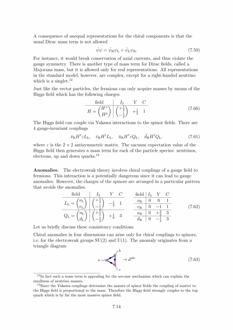
A consequence of unequal representations for the chiral components is that theusual Dirac mass term is not allowed

ψψ = ψRψL + ψLψR. (7.59)

For instance, it would break conservation of axial currents, and thus violate thegauge symmetry. There is another type of mass term for Dirac fields, called aMajorana mass, but it is allowed only for real representations. All representationsin the standard model, however, are complex, except for a right-handed neutrinowhich is a singlet.12

Just like the vector particles, the fermions can only acquire masses by means of theHiggs field which has the following charges:

field I3 Y C

H =

(H+

H0

) (+1

2

−12

)+1

21

(7.60)

The Higgs field can couple via Yukawa interactions to the spinor fields. There are4 gauge-invariant couplings

νRHTεLL, eRH

†LL, uRHTεQL, dRH

†QL, (7.61)

where ε is the 2× 2 antisymmetric matrix. The vacuum expectation value of theHiggs field then generates a mass term for each of the particle species: neutrinos,electrons, up and down quarks.13

Anomalies. The electroweak theory involves chiral couplings of a gauge field tofermions. This interaction is a potentially dangerous since it can lead to gaugeanomalies. However, the charges of the spinors are arranged in a particular patternthat avoids the anomalies.

field I3 Y C

LL =

(νL

eL

) (+1

2

−12

)−1

21

QL =

(uL

dL

) (+1

2

−12

)+1

63

field I3 Y C

νR 0 0 1

eR 0 −1 1

uR 0 +23

3

dR 0 −13

3

(7.62)

Let us briefly discuss these consistency conditions.

Chiral anomalies in four dimensions can arise only for chiral couplings to spinors,i.e. for the electroweak groups SU(2) and U(1). The anomaly originates from atriangle diagram

a

b

c

→ dabc (7.63)

12In fact such a mass term is appealing for the see-saw mechanism which can explain thesmallness of neutrino masses.

13Since the Yukawa couplings determine the masses of spinor fields the coupling of matter tothe Higgs field is proportional to the mass. Therefore the Higgs field strongly couples to the topquark which is by far the most massive spinor field.

7.14

which is proportional to some symmetric structure dabc of the three involved gaugefields. However, there is no anomaly for SU(2) alone because there is no symmetricstructure constants dabc in this group. The symmetric structure dabc trivially existsonly for the abelian group U(1). Moreover, there are anomalies for combinedgroups. Here, one of indices of dabc belongs to U(1), the other two to thesymmetric invariant form kbc. These mixed anomalies can arise for U(1)× SU(2)and for U(1)× SU(3). Finally, there a mixed anomaly between U(1) and gravity. Ifany of these anomalies is realised, one of the involved gauge symmetries would bebadly broken in the quantum theory.

Consider first the pure U(1) anomaly. We have to sum over all spinors propagatingin the loop. At each coupling a factor of the hypercharge is inserted. Hence theoverall contribution to the anomaly is proportional to

AU(1) ∼ TrL Y3 − TrR Y

3. (7.64)

This combination surprisingly equals zero

2 · 1(−12)3 + 2 · 3(+1

6)3 − (0)3 − (−1)3 − 3(+2

3)3 − 3(−1

3)3 = 0. (7.65)

The next anomaly mixes U(1) and SU(2). Only the left-handed lepton and quarkdoublets couple to SU(2), and they couple with the same strength. The thirdcoupling is the hypercharge, hence the anomaly is proportional to

AU(1)×SU(2) ∼ TrL Y (7.66)

Here we find zero(−1

2) + 3(−1

2) = 0. (7.67)

There is a mixed anomaly of U(1) and the SU(3) of quantum chromodynamics.This one involves only the quarks. Since the quarks all transform in the samefundamental representation, we only need to sum over the hypercharges

AU(1)×SU(3) ∼ TrQ,L Y − TrQ,R Y. (7.68)

Again, this combination equals zero

2(+16)− (+2

3)− (−1

3) = 0. (7.69)

Finally, there is a potential mixed gravitational anomaly. Gravity is not part ofthe electroweak theory or the standard model, so we need no pay attention to thisanomaly. Nevertheless, let us investigate it. Gravity couples to all particles withequal strength, so here we find

AU(1)×gravity ∼ TrL Y − TrR Y. (7.70)

This equals

2(−12) + 2 · 3(−1

2)− (0)− (−1)− 3(+2

3)− 3(−1

3) = 0. (7.71)

7.15

It is interesting to observe that there is no gravitational anomaly. Hence, theelectroweak theory can be consistently coupled to non-trivial gravitationalbackgrounds or even to quantum gravity (as far as that makes sense on its own).

The anomaly cancellations are rather curious. They could be interpreted in severalways:

• The structure of the standard model is actually constrained much more than itmay seem at first sight. In particular, the fact that there are three colours forthe strong nuclear interactions does play a significant role.14

• The standard model may be embedded into some theory with a larger symmetrygroup at higher energies, a so-called grand unified theory, where the anomalycancellations are more evident.

14In fact, the required invariance of Yukawa couplings implies several anomaly cancellations.Therefore, the cancellation of mixed anomalies are a consequence of the quarks and leptons beingmassive.

7.16