Embed Size (px)
Citation preview

QUANTUM MECHANICAL COMPUTATION OF BILLIARD SYSTEMS WITH
ARBITRARY SHAPES
INCI ERHAN
DECEMBER 2003
QUANTUM MECHANICAL COMPUTATION OF BILLIARD SYSTEMS WITH
ARBITRARY SHAPES
A THESIS SUBMITTED TO
THE GRADUATE SCHOOL OF NATURAL AND APPLIED SCIENCES
OF
THE MIDDLE EAST TECHNICAL UNIVERSITY
BY
INCI ERHAN
IN PARTIAL FULFILLMENT OF THE REQUIREMENTS FOR THE DEGREE OF
DOCTOR OF PHILOSOPHY
IN
THE DEPARTMENT OF MATHEMATICS
DECEMBER 2003
Approval of the Graduate School of Natural and Applied Sciences
Prof. Dr. Canan OZGEN
Director
I certify that this thesis satisfies all the requirements as a thesis for the degree of
Doctor of Philosophy.
Prof. Dr. Safak ALPAY
Head of Department
This is to certify that we have read this thesis and that in our opinion it is fully
adequate, in scope and quality, as a thesis for the degree of Doctor of Philosophy.
Prof. Dr. Hasan TASELI
Supervisor
Examining Committee Members
Prof. Dr. Hasan TASELI
Prof. Dr. Munevver TEZER
Prof. Dr. Marat AKHMET
Assoc. Prof. Dr. Hakan TARMAN
Assoc. Prof. Dr. N. Abdulbaki BAYKARA
Abstract
QUANTUM MECHANICAL COMPUTATION OF
BILLIARD SYSTEMS WITH ARBITRARY SHAPES
Inci Erhan
Ph.D., Department of Mathematics
Supervisor: Prof. Dr. Hasan TASELI
December 2003, 88 pages
An expansion method for the stationary Schrodinger equation of a particle moving
freely in an arbitrary axisymmetric three dimensional region defined by an analytic
function is introduced. The region is transformed into the unit ball by means of co-
ordinate substitution. As a result the Schrodinger equation is considerably changed.
The wavefunction is expanded into a series of spherical harmonics, thus, reducing
the transformed partial differential equation to an infinite system of coupled ordi-
nary differential equations. A Fourier-Bessel expansion of the solution vector in terms
of Bessel functions with real orders is employed, resulting in a generalized matrix
eigenvalue problem.
The method is applied to two particular examples. The first example is a pro-
late spheroidal billiard which is also treated by using an alternative method. The
numerical results obtained by both methods are compared. The second example is a
billiard family depending on a parameter. Numerical results concerning the second
example include the statistical analysis of the eigenvalues.
Keywords: Billiard Systems, Schrodinger Equation, Eigenfunction Expansion, Eigen-
value Problem, Spherical Harmonics
iii

Oz
KEYFI SEKILLI BILARDO SISTEMLERININ KUANTUM
MEKANIKSEL HESAPLAMALARI
Inci Erhan
Doktora, Matematik Bolumu
Tez Yoneticisi: Prof. Dr. Hasan TASELI
Aralık 2003, 88 sayfa
Analitik bir fonksiyon ile tanımlanan ve donel simetrisi olan keyfi bir uc boyutlu
bolgede, serbest hareket eden bir parcacıgın Schrodinger denklemi icin acılım yontemi
verilmektedir. Bir koordinat donusumu vasıtası ile bolge birim kureye donusturul-
mektedir. Bunun sonucunda, Schrodinger denklemi de onemli olcude degisiklige
ugramaktadır. Dalga fonksiyonu kuresel harmonikler cinsinden seriye acılmaktadır
ve boylece, degismis olan kısmi diferansiyel denklemi sonsuz boyutlu bir diferan-
siyel denklem sistemine indirgemektedir. Cozum vektoru icin reel mertebeli Bessel
fonksiyonları cinsinden Fourier-Bessel acılimları kullanilmaktadır ve denklem sistemi
genellestirilmis bir matris ozdeger problemine donusturulmektedir.
Yontem iki ozel ornege uygulanmaktadır. Birinci ornek “prolate spheroid” sek-
lindeki bilardo sistemidir ve ayni anda alternatif bir yontemle daha incelenmektedir.
Her iki yontemle elde edilen sayısal sonuclar karsılastırılmaktadır. Ikinci ornek bir
parametreye baglı bir bilardo ailesidir. Bu ornege ait sayısal sonuclar ozdegerlerin
istatistiksel analizini de icermektedir.
Anahtar Kelimeler: Bilardo Sistemleri, Schrodinger Denklemi, Ozfonksiyon Acı
lımı, Ozdeger Problemi, Kuresel Harmonikler
iv

To my lovely Selin,
v
Acknowledgments
I would like to express my sincere gratitude to my supervisor, Prof. Dr. Hasan
TASELI, for his precious guidance and encouragement throughout the research and
also for his friendly attitude. I would like to thank Prof. Dr. Munevver Tezer,
Assoc. Prof. Dr. N. A. Baki Baykara, Assoc. Prof. Dr. Hakan Tarman and Prof.
Dr. Marat Akhmet for their valuable suggestions. I also thank Christine Bockmann,
Arkadi Pikovsky and all the members of the Institute of Numerical Mathematics and
the Department of Nonlinear Dynamics in Potsdam University. I would also like to
express my thanks to the members of TUBITAK-BAYG for the grant which gave
me the possibility to join the study group in Potsdam University and especially to
Ayse Atas for her helps.
I offer my special thanks to my mother Gulten Muftuoglu, my father Fehmi Muf-
tuoglu for their love throughout my whole life. I especially thank my husband Adem
Tarık Erhan for his precious love, and encouragement during my long period of
study. I also thank my mother-in-law Necla Erhan who helped me by taking care of
my daughter during the period of preparing and writing the thesis.
I thank all the members of the Department of Mathematics and my friends for their
suggestions.
Last, but not least, I deeply thank my friend Omur Ugur for his helps during the
period of writing this thesis.
vi
Table of Contents
Abstract . . . . . . . . . . . . . . . . . . . . . . . . . . . . . . . . . . . . . . . . . . . . . . . . . . . . . iii
Oz . . . . . . . . . . . . . . . . . . . . . . . . . . . . . . . . . . . . . . . . . . . . . . . . . . . . . . . . . . . . . iv
Acknowledgments . . . . . . . . . . . . . . . . . . . . . . . . . . . . . . . . . . . . . . . . . . . vi
Table of Contents . . . . . . . . . . . . . . . . . . . . . . . . . . . . . . . . . . . . . . . . . . vii
CHAPTER
1 INTRODUCTION . . . . . . . . . . . . . . . . . . . . . . . . . . . . . . . . . . . . . . . . . 1
1.1 Billiard systems in classical and quantum mechanics . . . . . . . . . . 2
1.2 Statistical Properties of the Energy Spectra of Quantum Systems and
Random Matrix Theory . . . . . . . . . . . . . . . . . . . . . . . . . 5
1.3 Mathematical Model of a Quantum Billiard System Defined by a
Shape Function . . . . . . . . . . . . . . . . . . . . . . . . . . . . . . 7
2 Development of a Method for Solving Three-Dimensional
Billiards . . . . . . . . . . . . . . . . . . . . . . . . . . . . . . . . . . . . . . . . . . . . . . . . . . . 10
2.1 The Shape Function and the New Coordinates . . . . . . . . . . . . . 10
2.2 An Eigenfunction Expansion for the Transformed Equation . . . . . . 14
2.3 Reduction to a System of Ordinary Differential Equations . . . . . . . 18
vii

2.4 Transformation of the Boundary and Square Integrability Conditions 21
2.5 The Special Case of Spherical Billiard and the Truncated System of
ODEs . . . . . . . . . . . . . . . . . . . . . . . . . . . . . . . . . . . 22
2.6 Investigation of the Coefficient Matrices . . . . . . . . . . . . . . . . 26
2.7 Truncated Solution in One Dimensional Subspace . . . . . . . . . . . 29
2.8 Reduction of the System to a Matrix Eigenvalue Problem . . . . . . . 31
3 Two Examples: Prolate Spheroid and a Parameter-
Depending Billiard . . . . . . . . . . . . . . . . . . . . . . . . . . . . . . . . . . . . . . . 38
3.1 Prolate Spheroidal Billiard: Solution by the Method of Chapter 2 . . 38
3.2 Prolate Spheroidal Billiard: Solution by the Method of Moszkowski . 42
3.3 A Billiard Family Depending on a Parameter: Classical and Quantum
Mechanics . . . . . . . . . . . . . . . . . . . . . . . . . . . . . . . . . 48
4 Numerical Results and Discussion . . . . . . . . . . . . . . . . . . . . . 56
4.1 Numerical Results for the Prolate Spheroidal Billiard . . . . . . . . . 56
4.2 Numerical Results for the δ-billiard . . . . . . . . . . . . . . . . . . . 66
4.3 Statistical analysis of the spectra . . . . . . . . . . . . . . . . . . . . 74
5 Conclusion . . . . . . . . . . . . . . . . . . . . . . . . . . . . . . . . . . . . . . . . . . . . . . . . 80
References . . . . . . . . . . . . . . . . . . . . . . . . . . . . . . . . . . . . . . . . . . . . . . . . . . . 82
Vita . . . . . . . . . . . . . . . . . . . . . . . . . . . . . . . . . . . . . . . . . . . . . . . . . . . . . . . . . . . 88
viii
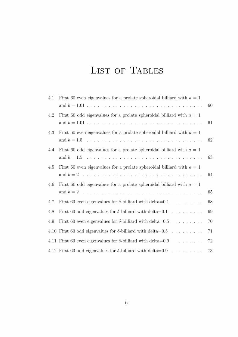
List of Tables
4.1 First 60 even eigenvalues for a prolate spheroidal billiard with a = 1
and b = 1.01 . . . . . . . . . . . . . . . . . . . . . . . . . . . . . . . . 60
4.2 First 60 odd eigenvalues for a prolate spheroidal billiard with a = 1
and b = 1.01 . . . . . . . . . . . . . . . . . . . . . . . . . . . . . . . . 61
4.3 First 60 even eigenvalues for a prolate spheroidal billiard with a = 1
and b = 1.5 . . . . . . . . . . . . . . . . . . . . . . . . . . . . . . . . 62
4.4 First 60 odd eigenvalues for a prolate spheroidal billiard with a = 1
and b = 1.5 . . . . . . . . . . . . . . . . . . . . . . . . . . . . . . . . 63
4.5 First 60 even eigenvalues for a prolate spheroidal billiard with a = 1
and b = 2 . . . . . . . . . . . . . . . . . . . . . . . . . . . . . . . . . 64
4.6 First 60 odd eigenvalues for a prolate spheroidal billiard with a = 1
and b = 2 . . . . . . . . . . . . . . . . . . . . . . . . . . . . . . . . . 65
4.7 First 60 even eigenvalues for δ-billiard with delta=0.1 . . . . . . . . 68
4.8 First 60 odd eigenvalues for δ-billiard with delta=0.1 . . . . . . . . . 69
4.9 First 60 even eigenvalues for δ-billiard with delta=0.5 . . . . . . . . 70
4.10 First 60 odd eigenvalues for δ-billiard with delta=0.5 . . . . . . . . . 71
4.11 First 60 even eigenvalues for δ-billiard with delta=0.9 . . . . . . . . 72
4.12 First 60 odd eigenvalues for δ-billiard with delta=0.9 . . . . . . . . . 73
ix
List of Figures
1.1 Two-Dimensional Region Generating an Axisymmetric Billiard . . . . 8
1.2 Three-Dimensional Axisymmetric Billiard. . . . . . . . . . . . . . . . 9
3.1 Prolate spheroid x2 + y2 +z2
(1.01)2≤ 1 . . . . . . . . . . . . . . . . . 41
3.2 Prolate spheroid x2 + y2 +z2
(1.5)2≤ 1 . . . . . . . . . . . . . . . . . . 41
3.3 Prolate spheroid x2 + y2 +z2
22≤ 1 . . . . . . . . . . . . . . . . . . . . 41
3.4 Classical Motion in Two-Dimensional Billiard . . . . . . . . . . . . . 49
3.5 Two-Dimensional δ-billiard with δ = 0.1 . . . . . . . . . . . . . . . . 50
3.6 Two-Dimensional δ-billiard with δ = 0.5 . . . . . . . . . . . . . . . . 50
3.7 Two-Dimensional δ-billiard with δ = 0.9 . . . . . . . . . . . . . . . . 50
3.8 Phase space of δ-billiard with δ = 0.1 . . . . . . . . . . . . . . . . . . 54
3.9 Phase space of δ-billiard with δ = 0.5 . . . . . . . . . . . . . . . . . . 54
3.10 Phase space of δ-billiard with δ = 0.9 . . . . . . . . . . . . . . . . . . 54
3.11 Three-Dimensional δ-billiard with δ = 0.1 . . . . . . . . . . . . . . . . 55
3.12 Three-Dimensional δ-billiard with δ = 0.5 . . . . . . . . . . . . . . . . 55
3.13 Three-Dimensional δ-billiard with δ = 0.9 . . . . . . . . . . . . . . . . 55
4.1 Nearest-Neighbor Spacing Histogram for even eigenvalues of the bil-
liard with δ=0.1. Solid line-Poisson distribution. Dashed line-GOE
distribution . . . . . . . . . . . . . . . . . . . . . . . . . . . . . . . . 77
x
4.2 Nearest-Neighbor Spacing Histogram for odd eigenvalues of the bil-
liard with δ=0.1. Solid line-Poisson distribution. Dashed line-GOE
distribution . . . . . . . . . . . . . . . . . . . . . . . . . . . . . . . . 77
4.3 Nearest-Neighbor Spacing Histogram for even eigenvalues of the bil-
liard with δ=0.5. Solid line-Poisson distribution. Dashed line- Brody
distribution with ν = 0.5 . . . . . . . . . . . . . . . . . . . . . . . . . 78
4.4 Nearest-Neighbor Spacing Histogram for odd eigenvalues of the bil-
liard with δ=0.5. Solid line-Poisson distribution. Dashed line- Brody
distribution with ν = 0.5 . . . . . . . . . . . . . . . . . . . . . . . . . 78
4.5 Nearest-Neighbor Spacing Histogram for even eigenvalues of the bil-
liard with δ=0.9. Solid line-Poisson distribution. Dashed line- Brody
distribution with ν = 0.9 . . . . . . . . . . . . . . . . . . . . . . . . . 79
4.6 Nearest-Neighbor Spacing Histogram for odd eigenvalues of the bil-
liard with δ=0.9. Solid line-Poisson distribution. Dashed line- Brody
distribution with ν = 0.9 . . . . . . . . . . . . . . . . . . . . . . . . . 79
xi
Chapter 1
INTRODUCTION
Investigation of quantum mechanical systems whose classical counterparts are chaotic
systems has received considerable interest in the last few decades. In classical me-
chanics, chaos is characterized by exponential instability with respect to the initial
conditions. The reason why such an exponentially unstable system is called chaotic
is that the motion is unpredictable. However, it took a long time trying to answer
the question how chaos in a classical system shows itself in the corresponding quan-
tum mechanical system. Unfortunately, this question still remains unanswered in the
sense of a rigorous theoretical analysis. On the other hand, numerical investigations
have given some very encouraging results.
In 1973 Percival [37] conjectured that the energy spectrum of a quantum system
whose classical analog is irregular (i.e., chaotic) is more sensitive to slowly changing
or fixed perturbations than those of a quantum system with regular (i.e., non chaotic)
classical counterpart. Pomphrey [38] showed that the idea worked well with the so
called Henon-Heiles potential.
Later, in order to shed more light on the relationship between classically chaotic
systems and their quantum analogs, scientists started to study the ”billiard” systems.
The billiard problems, that is, problems of free motion in a closed finite domain are
amongst the oldest problems in quantum mechanics, which have recently started
regaining remarkable interest [21, 42]. This is primarily due to the fact that these
simple systems, with only few exceptions, exhibit chaotic properties. In fact, de-
pending on the shape of the billiard, the motion of the particle inside can show a
rich variety of behaviors going from most regular to most chaotic.
1
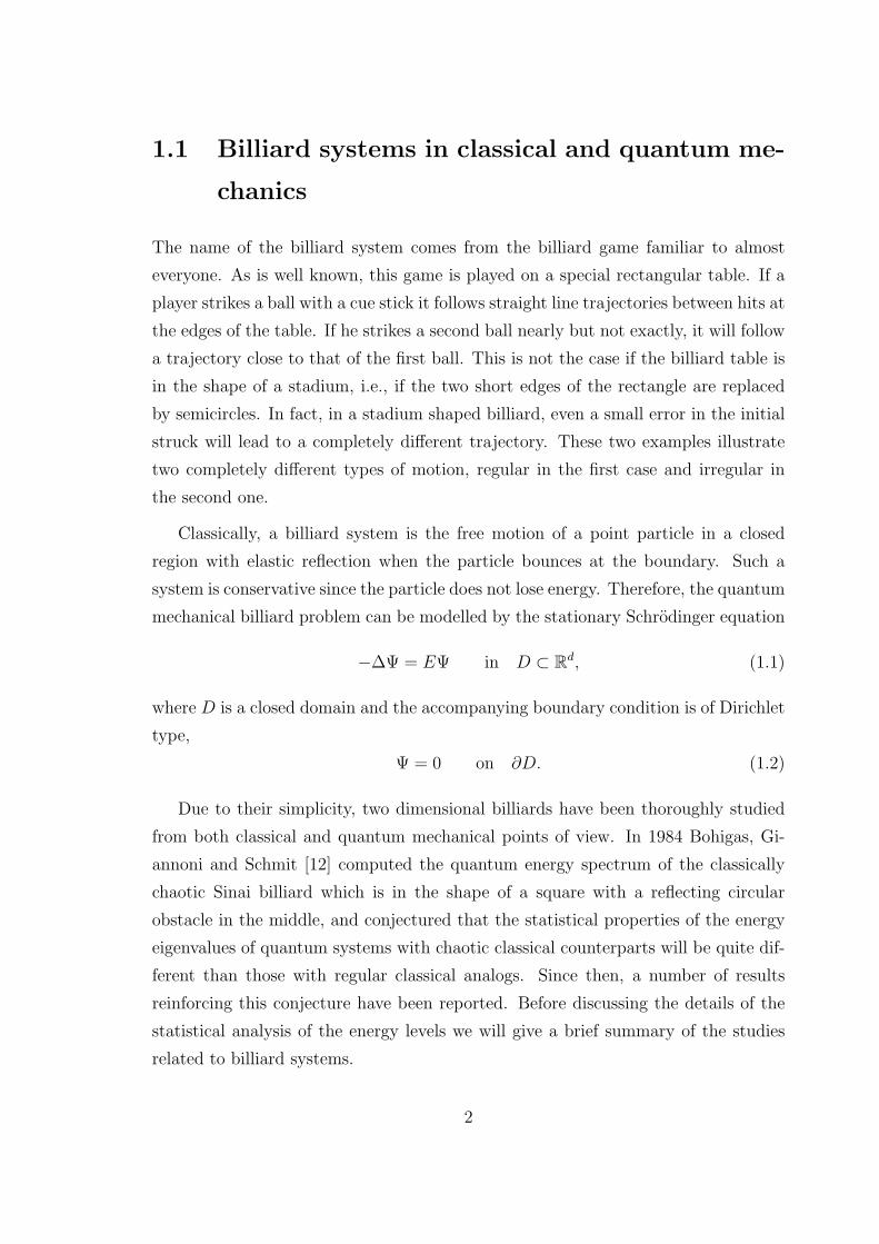
1.1 Billiard systems in classical and quantum me-
chanics
The name of the billiard system comes from the billiard game familiar to almost
everyone. As is well known, this game is played on a special rectangular table. If a
player strikes a ball with a cue stick it follows straight line trajectories between hits at
the edges of the table. If he strikes a second ball nearly but not exactly, it will follow
a trajectory close to that of the first ball. This is not the case if the billiard table is
in the shape of a stadium, i.e., if the two short edges of the rectangle are replaced
by semicircles. In fact, in a stadium shaped billiard, even a small error in the initial
struck will lead to a completely different trajectory. These two examples illustrate
two completely different types of motion, regular in the first case and irregular in
the second one.
Classically, a billiard system is the free motion of a point particle in a closed
region with elastic reflection when the particle bounces at the boundary. Such a
system is conservative since the particle does not lose energy. Therefore, the quantum
mechanical billiard problem can be modelled by the stationary Schrodinger equation
−∆Ψ = EΨ in D ⊂ Rd, (1.1)
where D is a closed domain and the accompanying boundary condition is of Dirichlet
type,
Ψ = 0 on ∂D. (1.2)
Due to their simplicity, two dimensional billiards have been thoroughly studied
from both classical and quantum mechanical points of view. In 1984 Bohigas, Gi-
annoni and Schmit [12] computed the quantum energy spectrum of the classically
chaotic Sinai billiard which is in the shape of a square with a reflecting circular
obstacle in the middle, and conjectured that the statistical properties of the energy
eigenvalues of quantum systems with chaotic classical counterparts will be quite dif-
ferent than those with regular classical analogs. Since then, a number of results
reinforcing this conjecture have been reported. Before discussing the details of the
statistical analysis of the energy levels we will give a brief summary of the studies
related to billiard systems.
2
Energy level statistics of the rectangular billiards have been given by Berry and
Tabor [10]. Spectral properties of the aforementioned stadium billiard , also called
Bunimovich stadium after the Russian scientist Bunimovich, have also been stud-
ied [13, 14]. Classical mechanics of an alternative stadium, the so called elliptical
stadium in which the semicircles in the stadium are replaced by semi-ellipses, has
been investigated recently [32]. Robnik has designed a family of plane billiards de-
fined by the conformal map of the unit disc in a complex plane w as follows,
B = {w | w = z + λz2, | z |≤ 1}, 0 ≤ λ ≤ 1
2(1.3)
Depending on values of λ, the shape of the billiard B varies from a circle to a
cardioid. Robnik studied this billiard family from both classical [43] and quantum
point of view [44, 41]. In another work by Backer and Steiner [4] the statistical
analysis of the energy spectra of the quantum cardioid billiard has been presented.
Perhaps one of the most popular billiard systems is the Sinai billiard. This system is
known to be classically chaotic and a detailed study of the corresponding quantum
mechanical system can be found in [12, 8]. Sieber and Steiner considered the motion
in a hyperbola billiard defined as follows,
B = {(x, y) | x ≥ 0, y ≥ 0, y ≤ 1
x}. (1.4)
They report that the hyperbola billiard is classically chaotic [45] and analyzed the
statistical properties of the energy spectra of the quantum hyperbola [46]. Another
one-parameter family of billiard systems has been studied recently both as classical
and quantum mechanical system. The boundary of this family has been defined by
the curve
y(x) = ±(1− | x |δ), x ∈ [−1, 1], 1 ≤ δ ≤ ∞, (1.5)
where the parameter δ determines the shape of the billiard. For δ=2 the shape of the
billiard is lemon-like, hence the billiard family has been called generalized parabolic
lemon shaped billiard [30]. Some results about quantum polygon billiard problem [27]
and rhombus billiard [17] has also been obtained. A survey on two dimensional
billiards can be found in [62]. Much less has been done on three-dimensional billiard
systems. There are only few results concerning the generalized three dimensional
stadium [36], three-dimensional Sinai billiard [39, 40] and conical billiard [28, 29].
3
The Schrodinger equation (1.1) is not exactly solvable unless the boundary of the
billiard is constant in some coordinate system. However, in order to perform a reli-
able statistical analysis one needs to compute hundreds of energy levels. Therefore
the use of efficient numerical methods gains a lot of significance. One of the most
practical methods is the boundary element method [24, 6]. This method uses integral
equation representation and discretization of the boundary which results in a homo-
geneous algebraic linear system. The zeros of the determinant give the eigenvalues.
This method has been widely used but has recently been shown to have problems if
the billiard is non-convex [26]. Another method is the point matching (collocation)
method, which uses an expansion of the wave function in suitable basis functions
and then forces this expansion to be zero on the discretized boundary [19, 20]. This
method has also a drawback as it can not be relied upon for accurate spectra. The
conformal mapping method is an elegant and efficient method which solves the bil-
liard problem by finding a suitable conformal mapping to transform the billiard to
the unit disc [41]. Unfortunately, the method can be applied only to two dimensional
billiards for which a conformal map can be found. The recently proposed constraint
operator method solves the billiard problem by using an enlarged billiard on which
the Schrodinger equation is exactly solvable and then ”cuts away” the unwanted part
of that billiard to obtain the original one [33]. It is interesting from both mathemati-
cal and physical points of view because it can represent the Hamiltonian of a chaotic
billiard by the eigenfunctions of a regular one. The method reduces the Schrodinger
equation to a matrix eigenvalue problem. A similar method, using an expansion
in eigenfunctions of square billiard has been proposed recently [25]. The scaling
method for computation of highly exited states of billiards [57] and the Korringa-
Kohn-Rostoker method [8] are also worth mentioning here. In some recent studies
two-dimensional quantum billiards have been studied experimentally by means of
microwave cavities [22, 47] and highly excited energy levels have been obtained in
this manner.
4
1.2 Statistical Properties of the Energy Spectra of
Quantum Systems and Random Matrix The-
ory
The pioneering work of Berry and Tabor [10] and the work of Bohigas, Giannoni
and Schmit [12] led to an enormous interest in the Random Matrix Theory (RMT)
developed by Wigner, Dyson, Mehta and others in 1950-1960. The most detailed
and complete monograph about RMT is the second enlarged edition of “Random
Matrices” written by Mehta [34].
The quantum mechanical system is represented by its Hamiltonian operator which
in turn can be represented by a Hermitian matrix. For billiard systems this matrix
is real symmetric and is invariant under orthogonal transformations. More precisely,
let H be the real symmetric matrix representation of the Hamiltonian operator in
any arbitrary basis. Then the matrix H′ defined by
H′ = OHOT (1.6)
is also real and symmetric, where O is an orthogonal matrix. If the system is regular
and the basis is suitably chosen, then the matrix H is diagonal. In this case the
eigenvalues of the system are not correlated. Denote the ordered eigenvalues by
E1 ≤ E2 ≤ E3 ≤ . . . ≤ EN ≤ . . ., and the spacings between them by si = Ei+1 −Ei,
i = 1, 2, 3, . . ., then it can be shown that the probability distribution function for
these spacings, the so-called Nearest Neighbor Spacing Distribution(NNSD) has the
form
p(s) = e−s. (1.7)
This is the well known Poisson distribution function. Hence, the NNSD of regular
systems is expected to be Poissonian. If the quantum system is not regular, then
the matrix H belongs to the Gaussian Orthogonal Ensemble(GOE) in RMT. Two
other ensembles: Gaussian Unitary(GUE) and Gaussian Symplectic(GSE) have to
be mentioned here, but none of them will be used in this work, so we will not discuss
them. The NNSD for the eigenvalues of matrices from the GOE can be obtained
from the joint probability density function by long integration and has the following
5
form
p(s) =π
2se−
π4s2
. (1.8)
Most classical billiards are neither completely regular nor completely chaotic. In
such systems, called generic, both types of motion co-exist. The NNSD of the energy
levels of generic systems is neither Poissonian nor like that of the GOE. Several
theoretical models have been developed for this class of systems. The first model
was introduced by Brody [50],
p(s) = (ν + 1)aνsν exp(−aνs
ν+1) (1.9)
where
aν =
[Γ
(ν + 2
ν + 1
)]ν+1
. (1.10)
For ν = 0, the Brody distribution reduces to Poissonian and for ν = 1 the NNSD of
the GOE is obtained. Another approach is that of Izrailev [23], who proposed the
following distribution,
p(s) = Asν exp
[−π2
16νs2 −
(C − ν
2
) π
2s
](1.11)
where the constants A and C can be obtained using normalization conditions. The
distribution becomes Poissonian for ν = 0, and it coincides with the NNSD of the
GOE for ν = 1. The derivation of the above distributions and some other theoretical
models interpolating between the Poisson and GOE cases can be found in a recent
monograph by Stockmann [48].
Other frequently used statistics are the Dyson-Mehta or spectral rigidity statistics
∆3 and the number variance Σ2. Definition and derivation of these statistics can be
found in [34] and [48], but will not be discussed here.
One of the two examples considered in this study is the integrable prolate sphe-
roidal billiard, the other is a generic billiard depending on a parameter. As it will be
shown in chapter 4, the NNSD of the numerically calculated spectra for the prolate
spheroid agrees with Poisson distribution (1.7), while for the second generic billiard
the NNSD is similar to Brody’s model (1.9). Unfortunately, due to computational
difficulties in evaluating the matrix elements of the Hamiltonian of the system, the
statistical analysis has been performed using a relatively small number of spacings,
however the resulting distribution properties have shown good agreement with the
predictions of Random Matrix Theory.
6
1.3 Mathematical Model of a Quantum Billiard
System Defined by a Shape Function
In this study we propose a numerical method for solving a quite general class of
axisymmetric three dimensional billiard systems obtained by rotating a closed finite
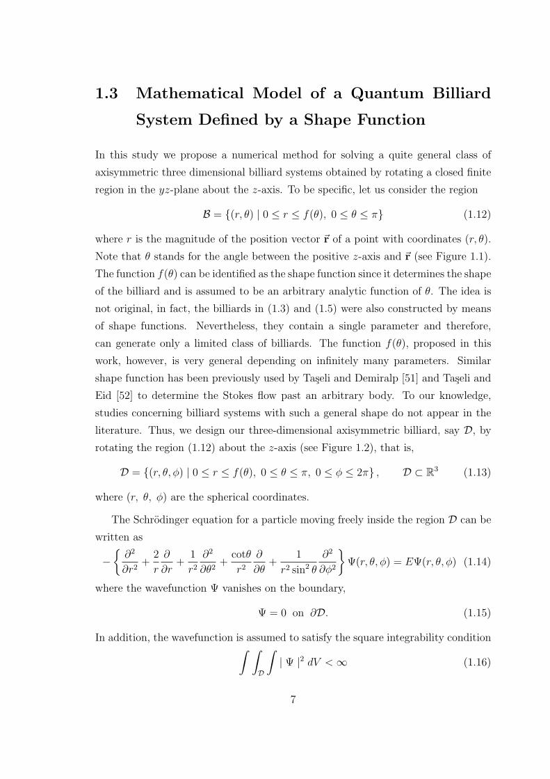
region in the yz-plane about the z-axis. To be specific, let us consider the region
B = {(r, θ) | 0 ≤ r ≤ f(θ), 0 ≤ θ ≤ π} (1.12)
where r is the magnitude of the position vector ~r of a point with coordinates (r, θ).
Note that θ stands for the angle between the positive z-axis and ~r (see Figure 1.1).
The function f(θ) can be identified as the shape function since it determines the shape
of the billiard and is assumed to be an arbitrary analytic function of θ. The idea is
not original, in fact, the billiards in (1.3) and (1.5) were also constructed by means
of shape functions. Nevertheless, they contain a single parameter and therefore,
can generate only a limited class of billiards. The function f(θ), proposed in this
work, however, is very general depending on infinitely many parameters. Similar
shape function has been previously used by Taseli and Demiralp [51] and Taseli and
Eid [52] to determine the Stokes flow past an arbitrary body. To our knowledge,
studies concerning billiard systems with such a general shape do not appear in the
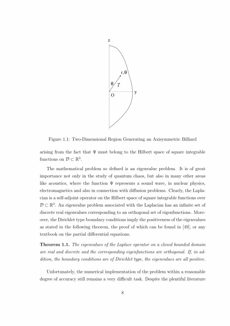
literature. Thus, we design our three-dimensional axisymmetric billiard, say D, by
rotating the region (1.12) about the z-axis (see Figure 1.2), that is,
D = {(r, θ, φ) | 0 ≤ r ≤ f(θ), 0 ≤ θ ≤ π, 0 ≤ φ ≤ 2π} , D ⊂ R3 (1.13)
where (r, θ, φ) are the spherical coordinates.
The Schrodinger equation for a particle moving freely inside the region D can be
written as
−{
∂2
∂r2+
2
r
∂
∂r+
1
r2
∂2
∂θ2+
cotθ
r2
∂
∂θ+
1
r2 sin2 θ
∂2
∂φ2
}Ψ(r, θ, φ) = EΨ(r, θ, φ) (1.14)
where the wavefunction Ψ vanishes on the boundary,
Ψ = 0 on ∂D. (1.15)
In addition, the wavefunction is assumed to satisfy the square integrability condition∫ ∫
D
∫| Ψ |2 dV < ∞ (1.16)
7
y
z
r
r,
θ
θ
O
Figure 1.1: Two-Dimensional Region Generating an Axisymmetric Billiard
arising from the fact that Ψ must belong to the Hilbert space of square integrable
functions on D ⊂ R3.
The mathematical problem so defined is an eigenvalue problem. It is of great
importance not only in the study of quantum chaos, but also in many other areas
like acoustics, where the function Ψ represents a sound wave, in nuclear physics,
electromagnetics and also in connection with diffusion problems. Clearly, the Lapla-
cian is a self-adjoint operator on the Hilbert space of square integrable functions over
D ⊂ R3. An eigenvalue problem associated with the Laplacian has an infinite set of
discrete real eigenvalues corresponding to an orthogonal set of eigenfunctions. More-
over, the Dirichlet type boundary conditions imply the positiveness of the eigenvalues
as stated in the following theorem, the proof of which can be found in [49], or any
textbook on the partial differential equations.
Theorem 1.1. The eigenvalues of the Laplace operator on a closed bounded domain
are real and discrete and the corresponding eigenfunctions are orthogonal. If, in ad-
dition, the boundary conditions are of Dirichlet type, the eigenvalues are all positive.
Unfortunately, the numerical implementation of the problem within a reasonable
degree of accuracy still remains a very difficult task. Despite the plentiful literature
8
Figure 1.2: Three-Dimensional Axisymmetric Billiard.
about its numerical treatment in two dimensions, results on the three-dimensional
case are only few. This is mainly due to the fact that solving three-dimensional
problems by means of the aforementioned methods is much more difficult than solving
two-dimensional ones. Moreover, some of the methods are applicable only in two
dimensions.
Therefore, the main objective of this study is to develop a method to deal nu-
merically with the problem (1.14)-(1.16). However, it will be made clear in the
forthcoming chapters that this thesis seems to be interesting from two different as-
pects. In other words, it has applications in both mathematics and physics. First,
it provides a numerical method for a quite general class of eigenvalue problems. Se-
cond, the general form of the shape function f(θ) makes it possible to design a wide
variety of three-dimensional billiards and investigate them not only as quantum but
also as classical systems.
9
Chapter 2
Development of a Method for
Solving Three-Dimensional
Billiards
2.1 The Shape Function and the New Coordinates
In this section we introduce a coordinate transformation which transforms the region
under consideration into the unit ball.
Consider again the billiard
D = {(r, θ, φ) | 0 ≤ r ≤ f(θ), 0 ≤ θ ≤ π, 0 ≤ φ ≤ 2π} (2.1)
where (r, θ, φ) are the usual spherical coordinates related to the rectangular coordi-
nates by x = r sin θ cos φ, y = r sin θ sin φ and z = r cos θ. The analyticity of f(θ)
suggests proposing a shape function of the form
f(θ) = 1 +∞∑
k=1
αk cosk θ, αk ∈ R (2.2)
where αk’s are regarded as the shape parameters. Note that, 1 ≤ f(θ) < ∞ must
hold for all θ ∈ [0, π] in order to have a bounded geometrical region. By means
of the flexible parameters αk introduced in (2.2), it is possible to deal with various
billiards including prolate and oblate spheroids, the three-dimensional version of the
cardioid billiard mentioned in Section 1.1 and many others. Furthermore, even very
10
simple choices of f(θ) like finite sums containing only few terms can generate plenty
of shapes. Note also that the particular case, in which αk = 0 for all k ∈ Z+,
corresponds to the exactly solvable spherical billiard.
We introduce the new coordinates
ξ =r
f(θ), ξ ∈ [0, 1]
η = cos θ, η ∈ [−1, 1](2.3)
where the third coordinate φ remains unchanged. The region D is now transformed
into
D = {(ξ, η, φ) | 0 ≤ ξ ≤ 1, −1 ≤ η ≤ 1, 0 ≤ φ ≤ 2π} , (2.4)
which is a unit ball. Partial derivative operators involved in the Schrodinger equation
take very complicated forms such that
∂
∂r=
1
F (η)
∂
∂ξ,
∂2
∂r2=
1
[F (η)]2∂2
∂ξ2,
∂
∂θ=
√1− η2
[F ′(η)
F (η)ξ
∂
∂ξ− ∂
∂η
]
and
∂2
∂θ2= (1− η2)
[F ′(η)]2
[F (η)]2ξ2 ∂2
∂ξ2− 2(1− η2)
F ′(η)
F (η)ξ
∂2
∂ξ∂η
−(1− η2)F ′′(η)F (η)− ηF ′(η)F (η)− 2(1− η2) [F ′(η)]2
[F (η)]2ξ
∂
∂ξ
+(1− η2)∂2
∂η2− η
∂
∂η
(2.5)
where the function F (η),
F (η) = 1 +∞∑
k=1
αkηk. (2.6)
is the shape function written in terms of the new variable η. Obviously, the coor-
dinate system (ξ, η, φ) is quite an unusual one, which is not orthogonal. This fact,
unfortunately, has some very unpleasant consequences as will be seen later. Never-
theless, in almost all studies summarized in Section 1.1 concerning quantum billiard
problems even in two dimensions, serious difficulties of one kind or other have been
encountered.
Let us recall our mathematical problem consisting of the Schrodinger equation
and the additional conditions in (1.14)-(1.16). We employ the substitutions in (2.3)
11
and partial derivatives in (2.5) to transform the Schrodinger equation to a new partial
differential equation. Thus, we get
−{[
1
F 2+ (1− η2)
(F ′)2
F 4
]∂2
∂ξ2− 2(1− η2)
F ′
F 3
1
ξ
∂2
∂ξ∂η
+
[2
F 2+
2(1− η2) (F ′)2 − (1− η2)F ′′F + 2ηF ′FF 4
]1
ξ
∂
∂ξ
+1
F 2ξ2
[(1− η2)
∂2
∂η2− 2η
∂
∂η− 1
1− η2
∂2
∂φ2
]}Ψ(ξ, η, φ) = EΨ(ξ, η, φ)
which becomes
−{[
F 2 + (1− η2) (F ′)2] ∂2
∂ξ2− 2(1− η2)F ′F
1
ξ
∂2
∂ξ∂η
+[2F 2 + 2(1− η2) (F ′)2 − (1− η2)F ′′F + 2ηF ′F
] 1
ξ
∂
∂ξ
+F 2
ξ2
[(1− η2)
∂2
∂η2− 2η
∂
∂η− 1
1− η2
∂2
∂φ2
]}Ψ(ξ, η, φ) = EF 4Ψ(ξ, η, φ)
(2.7)
upon multiplication of both sides by F 4, where we have dropped the η-dependance
of the shape function F (η) for simplicity. The resulting partial differential equation
cannot be treated by the method of separation of variables. In fact, it is completely
different from the original one, since the shape function has been inserted into it. As a
result, shape effects are now characterized mainly by the partial differential equation.
However, this new equation will be solved in the standardized region (2.4), i.e., in
the unit ball. It seems that an expansion method for the wavefunction will be more
appropriate.
The Jacobian determinant of the transformation (2.3) is
∂(ξ, η, φ)
∂(r, θ, φ)=
∣∣∣∣∣∣∣∣
1f(θ)
−r f ′(θ)f2(θ)
0
0 − sin θ 0
0 0 1
∣∣∣∣∣∣∣∣= −sin θ
f(θ)
leading to a square integrability condition of the form∫ 2π
0
∫ 1
−1
∫ 1
0
|Ψ(ξ, η, φ)|2 ξ2 [F (η)]3 dξdηdφ < ∞. (2.8)
12
over the new region. As is shown, this square integrability condition contains the
unspecified shape function as a weight. More precisely, (2.8) implies that the wave-
function must belong to the Hilbert space of square integrable functions over D under
the weight ξ2 [F (η)]3. Thus, to find a suitable expansion basis becomes a very dif-
ficult task. However, from the definition of F (η), it follows that 1 ≤ F (η) for all
η ∈ [−1, 1], and therefore,
∫ 2π
0
∫ 1
−1
∫ 1
0
|Ψ(ξ, η, φ)|2 ξ2dξdηdφ ≤∫ 2π
0
∫ 1
−1
∫ 1
0
|Ψ(ξ, η, φ)|2 ξ2 [F (η)]3 dξdηdφ
(2.9)
implying the boundedness of the integral
∫ 2π
0
∫ 1
−1
|Ψ(ξ, η, φ)|2 dηdφ < ∞, (2.10)
for every fixed ξ ∈ (0, 1]. In what follows, (2.10) suggests that Ψ(ξ, η, φ) can also
be regarded as a square integrable function over the region [−1, 1]× [0, 2π] with the
unit weight for a fixed ξ. In fact, this region represents a sphere of radius ξ defined
by
Dξ = {(ξ, η, φ)|ξ = c,−1 ≤ η ≤ 1, 0 ≤ φ ≤ 2π} (2.11)
where ξ is assumed to be constant.
Let us now consider the differential operator
T = (1− η2)∂2
∂η2− 2η
∂
∂η− 1
1− η2
∂2
∂φ2(2.12)
appearing on the last term of the left hand side of (2.7). The eigenvalue problem
related to this operator, i.e.,
T y = λy (2.13)
generates the orthogonal sequence of the spherical harmonics defined as [15]
Y nm(η, φ) = P |n|
m (η)einφ (2.14)
corresponding to the eigenvalues λ = −m(m + 1), where the indices range over
−m ≤ n ≤ m, 0 ≤ m ≤ ∞. Here the functions P|n|m (η) are the associated Legendre
functions of the first kind. As a matter of fact, (2.13) has also solutions of the form
Q|n|m (η)einφ, where the Q
|n|m (η) denote the associated Legendre functions of the second
13
kind. However, these functions are not bounded at η = ±1, and, therefore, they are
not suitable as an expansion basis for our problem.
We now give the following theorems which complete the analysis related to the
choice of an expansion basis.
Theorem 2.1. The system of spherical harmonics {Y nm}, where m = 0, 1, . . .∞,
−m ≤ n ≤ m is complete.
Theorem 2.2. Every function, square integrable over a sphere can be expanded in
terms of spherical harmonics.
The proofs of Theorems 2.1 and 2.2 can be found in [15] or [56].
2.2 An Eigenfunction Expansion for the Trans-
formed Equation
In this section, we propose an expansion in spherical harmonics for the wavefunction
Ψ(ξ, η, φ) and insert this expansion into the transformed equation. The discussion
of the previous section demonstrates the advantage of using such an expansion, for,
it is clear that this expansion will replace the differential operator in (2.12) by its
eigenvalues. Thus, we assume
Ψ(ξ, η, φ) =∞∑
m=0
m∑n=−m
χnm(ξ)P |n|
m (η)einφ
where the χnm(ξ) denote the Fourier coefficient functions. It is more appropriate for
our analysis to rewrite this expansion as
Ψ(ξ, η, φ) =∞∑
m=0
{Φ0
m(ξ)P 0m(η) +
m∑n=1
[Φnm(ξ) cos nφ + ψn
m(ξ) sin nφ] P nm(η)
}(2.15)
where now the expansion coefficients are the Φnm and ψn
m. Theorems 2.1 and 2.2
together with the condition (2.10) imply that this expansion converges in the mean
to the function Ψ(ξ, η, φ) for every fixed ξ ∈ (0, 1], provided that the Φnm(ξ) and
14
ψnm(ξ) are the Fourier coefficients defined by
Φ0m(ξ) =
1
4π
2
(2m + 1)
∫ 2π
0
∫ 1
−1
Ψ(ξ, η, φ)P 0m(η)dηdφ
Φnm(ξ) =
1
2π
2
(2m + 1)
(m + n)!
(m− n)!
∫ 2π
0
∫ 1
−1
Ψ(ξ, η, φ)P nm(η) cos nφdηdφ
and
ψnm(ξ) =
1
2π
2
(2m + 1)
(m + n)!
(m− n)!
∫ 2π
0
∫ 1
−1
Ψ(ξ, η, φ)P nm(η) sin nφdηdφ
(2.16)
respectively, for n = 1, 2, . . . , m and m = 0, 1, 2, . . . ,∞.
Before proceeding, let us have a closer look at the shape function F (η). From
a computational point of view, the power series representation of F (η) should be
truncated. Therefore, we use the truncated shape function, say G(η),
G(η) = 1 +K∑
k=1
αkηk. (2.17)
instead of the original shape function unless F (η) is already defined by a finite sum.
Note that,
F (η) = limK→∞
G(η).
In what follows, we will replace the function F (η) in the equation (2.7) by G(η).
Remark 1. In order to have a “numerically” convergent algorithm it is important
that the power series describing F (η) converges very rapidly, i.e., the coefficients
αk form a rapidly decreasing sequence, Otherwise, one must take a large truncation
order K which will cause long computing time, large memory and may even lead to
a divergent algorithm. ♦We shall make the following definitions for the sake of brevity
G0(η) := [G(η)]2
G1(η) := [G(η)]2 + (1− η2) [G′(η)]2
G2(η) := 2ηG′(η)G(η)
G3(η) := (1− η2)G′′(η)G(η).
(2.18)
It follows easily from the definition of G(η) that all the functions Gi(η) where i =
0, 1, 2, 3, are polynomials of degree 2K in η. We employ (2.18) and (2.12) to rewrite
15
equation (2.7) as
−{G1(η)
∂2
∂ξ2+ [2G1(η) + G2(η)− G3(η)]
1
ξ
∂
∂ξ− (1− η2)
ξηG2(η)
∂2
∂ξ∂η
+G0(η)
ξ2T
}Ψ(ξ, η, φ) = E [G0(η)]2 Ψ(ξ, η, φ).
(2.19)
Substituting the expansion (2.15) in equation (2.19) and using (2.13) we obtain
−∞∑
m=0
m∑n=0
{G1(η)P n
m(η)d2
dξ2Φn
m(ξ) + [2G1(η) + G2(η)− G3(η)]1
ξ
d
dξΦn
m(ξ)
−G2(η)
η(1− η2)
d
dηP n
m(η)1
ξ
d
dξΦn
m(ξ)−m(m + 1) G0(η)P nm(η)
1
ξ2Φn
m(ξ)
}cos nφ
−∞∑
m=0
m∑n=1
{G1(η)P n
m(η)d2
dξ2ψn
m(ξ) + [2G1(η) + G2(η)− G3(η)]1
ξ
d
dξψn
m(ξ)
−G2(η)
η(1− η2)
d
dηP n
m(η)1
ξ
d
dξψn
m(ξ)−m(m + 1) G0(η)P nm(η)
1
ξ2ψn
m(ξ)
}sin nφ
= E
∞∑m=0
{[G0(η)]2
m∑n=0
P nm(η)Φn
m(ξ) cos nφ +m∑
n=1
P nm(η)ψn
m(ξ) sin nφ
}.
(2.20)
The range of the index n of the inner sums involved in this equation depends on
the index m of the outer sums, otherwise one could easily get rid of one summation
using the orthogonality of the trigonometric functions over [0, 2π]. On the other
hand, notice that, one can reorder the two double sums as∞∑
n=0
∞∑m=n
and∞∑
n=1
∞∑m=n
respectively, bearing in mind the relation between the indices n and m. Then we
multiply (2.20) by cos nφ for n = 0, 1, . . . and by sin nφ for n = 1, 2, . . . and integrate
with respect to φ over [0, 2π]. This yields
−∞∑
m=n
{G1(η)P n
m(η)d2
dξ2Φn
m(ξ) + [2G1(η) + G2(η)− G3(η)] P nm(η)
1
ξ
d
dξΦn
m(ξ)
−G2(η)
η(1− η2)
d
dηP n
m(η)1
ξ
d
dξΦn
m(ξ)−m(m + 1) G0(η)P nm(η)
1
ξ2Φn
m(ξ)
}
= E
∞∑m=n
[G0(η)]2 P nm(η)Φn
m(ξ)
(2.21)
16
for n = 0, 1, 2, . . . and
−∞∑
m=n
{G1(η)P n
m(η)d2
dξ2ψn
m(ξ) + [2G1(η) + G2(η)− G3(η)] P nm(η)
1
ξ
d
dξψn
m(ξ)
−G2(η)
η(1− η2)
d
dηP n
m(η)1
ξ
d
dξψn
m(ξ)−m(m + 1) G0(η)P nm(η)
1
ξ2ψn
m(ξ)
}
= E
∞∑m=n
[G0(η)]2 P nm(η)ψn
m(ξ)
(2.22)
for n = 1, 2, . . . in the virtue of the orthogonality of the trigonometric functions.
The two equation sets (2.21) and (2.22) for the Fourier coefficient functions Φnm
and ψnm are independent of each other. This is a result of the axial symmetry of the
region which allows a separation of the expansion (2.15) into two parts containing
even and odd eigenfunctions in φ. Moreover (2.21) and (2.22) are identical for each
n ∈ Z+, i.e., Φnm(ξ) = ψn
m(ξ) for n ∈ Z+. Hereafter, we consider only the equations
for Φnm(ξ). By means of the differential-difference relation [1]
(1− η2)∂
∂ηP n
m(η) = (m + 1)ηP nm(η)− (m− n + 1)P n
m+1(η)
it is possible to get rid of the derivative of P nm(η) and obtain
−∞∑
m=n
{G1(η)P n
m(η)d2
dξ2Φn
m(ξ) + [G1(η)−mG2(η)− G3(η)] P nm(η)
1
ξ
d
dξΦn
m(ξ)
+G2(η)
η(m− n + 1)P n
m+1(η)1
ξ
d
dξΦn
m(ξ)−m(m + 1)G0(η)P nm(η)
1
ξ2Φn
m(ξ)
}
= E
∞∑m=n
[G0(η)]2 P nm(η)Φn
m(ξ)
(2.23)
for every n = 0, 1, 2, . . .. In our further analysis we will treat equation (2.23) for a
fixed n keeping in mind that n = 0, 1, ....
17
2.3 Reduction to a System of Ordinary Differen-
tial Equations
An eigenfunction expansion of the type (2.15) makes it possible to reduce a partial
differential equation to a system of ordinary differential equations [54, 16]. The
technical details of such a reduction, which leads to an infinite system of coupled
ordinary differential equations for the functions Φnm(ξ) will be introduced in this
section.
Let us consider the η-dependent expressions in equation (2.23). The polynomials
Gi(η) involved in these expressions can be written as
Gi(η) =2K∑
k=0
gi,kηk (2.24)
for i = 0, 1, 2, 3. Rewriting the truncated shape function G(η) in the form G(η) =K∑
k=0
αkηk, where α0 = 1 and using the definitions of Gi(η) given in (2.18), we compute
the coefficients gi,k as
g0,k =k∑
t=0
αtαk−t k = 0, 1, . . . , 2K
g1,k =k∑
t=0
αtαk−t + (t + 1)(k − t + 1)αt+1αk−t+1 k = 0, 1
g1,k =k∑
t=0
αtαk−t + (t + 1)(k − t + 1)αt+1αk−t+1
−k−2∑t=0
(t + 1)(k − t− 1)αt+1αk−t−1 k = 2, 3, . . . , 2K − 2
g1,k =k∑
t=0
αtαk−t −k−2∑t=0
(t + 1)(k − t− 1)αt+1αk−t−1 k = 2K − 1, 2K
g2,0 = 0
g2,k = 2k∑
t=0
(k − t + 1)αtαk−t+1 k = 1, 2, . . . , 2K
18
g3,k =k∑
t=0
(k − t + 1)(k − t + 2)αtαk−t+2 k = 0, 1
g3,k =k∑
t=0
(k − t + 1)(k − t + 2)αtαk−t+2
−k−2∑t=0
(k − t− 1)(k − t)αtαk−t k = 2, 3, . . . , 2K − 2
g3,k = −k−2∑t=0
(k − t− 1)(k − t)αtαk−t k = 2K − 1, 2K
(2.25)
where clearly α0 = 1 and αr = 0 for all r = K+1, K+2, . . . , 2K. The right-hand-side
of (2.23) contains [G0(η)]2, which can be explicitly written as
[G0(η)]2 =4K∑
k=0
g4,kηk, g4,k =
k∑t=0
g0,tg0,k−t, k = 0, 1, . . . , 4K. (2.26)
Now, using (2.24) and (2.26), we rewrite equation (2.23) in the form
−∞∑
m=n
{[2K∑
k=0
g1,kηkP n
m(η)
]d2
dξ2Φn
m(ξ)
+
[2K∑
k=0
(2g1,k −mg2,k − g3,k) ηkP nm(η) + (m− n + 1)
2K−1∑
k=0
g2,k+1ηkP n
m+1(η)
]1
ξ
d
dξΦn
m(ξ)
−m(m + 1)
[2K∑
k=0
g0,kηkP n
m(η)
]1
ξ2Φn
m(ξ)
}= E
∞∑m=n
{[4K∑
k=0
g4,kηkP n
m(η)
]Φn
m(ξ)
}
(2.27)
The product ηkP nm(η) can be expanded into a series of P n
l (η),
ηkP nm(η) =
∞∑
l=n
γ(n)l,m,kP
nl (η), (2.28)
where
γ(n)m,l,k =
∫ 1
−1
ηkP nm(η)P n
l (η)dη. (2.29)
Evaluation of the coefficients γ(n)l,m,k is much easier than it looks, thanks to the recur-
rence relation of the associated Legendre functions [7],
ηP nm(η) =
m− n + 1
2m + 1P n
m+1 +m + n
2m + 1P n
m−1. (2.30)
Clearly, the computation of γ(n)l,m,0 is sufficient to obtain all the other coefficients γ
(n)l,m,k
up to any desired degree k. The orthogonality relation of the associated Legendre
19
functions on the other hand, determines γ(n)l,m,0 as
γ(n)l,m,0 =
∫ 1
−1
P nm(η)P n
l (η)dη =2
(2m + 1)
(m + n)!
(m− n)!δl,m (2.31)
where δl,m stands for Kronecker’s delta. We employ (2.28) and define the matrices
An :=[an
l,m
], Bn :=
[bnl,m
], Cn :=
[cnl,m
]and Dn :=
[dn
l,m
]with entries
anl,m =
2K∑
k=0
g1,kγ(n)l,m,k
bnl,m =
2K∑
k=0
(2g1,k −mg2,k − g3,k) γ(n)l,m,k + (m− n + 1)
2K−1∑
k=0
g2,k+1γ(n)l,m+1,k
cnl,m = m(m + 1)
2K∑
k=0
g0,kγ(n)l,m,k
dnl,m =
4K∑
k=0
g4,kγ(n)l,m,k
(2.32)
where n is fixed. Notice that in the definition of the matrices, the superscript “n” is
used merely as a notation and cannot mean the power. Thus, equation (2.27) turns
out to be
∞∑
l=n
{ ∞∑m=n
[an
l,m
d2
dξ2Φn
m(ξ) + bnl,m
1
ξ
d
dξΦn
m(ξ)− cnl,m
1
ξ2Φn
m(ξ) + Ednl,mΦn
m(ξ)
]}P n
l (η) = 0.
Since the set{P n
n (η), P nn+1(η), P n
n+2(η), . . .}
is linearly independent for a fixed n, we
must have
∞∑m=n
[an
l,m
d2
dξ2Φn
m(ξ) + bnl,m
1
ξ
d
dξΦn
m(ξ)− cnl,m
1
ξ2Φn
m(ξ) + Ednl,mΦn
m(ξ)
]= 0, (2.33)
for each l = n, n + 1, . . ., and fixed n. That is, we obtain an infinite system of cou-
pled ordinary differential equations for the determination of the coefficient functions
Φnn(ξ), Φn
n+1(ξ), . . .. In matrix-vector form the system is written as
{An d2
dξ2+ Bn 1
ξ
d
dξ−Cn 1
ξ2
}Φn = −EDnΦn (2.34)
where Φn stands for the vector
Φn =[Φn
n(ξ), Φnn+1(ξ), Φ
nn+2(ξ), . . .
]T. (2.35)
20
This vector differential equation cannot have an exact analytical solution unless the
matrices An, Bn, Cn and Dn are diagonal. Then the ordinary differential equations
(ODEs) will be uncoupled, i.e., they will be independent of each other. Unfortu-
nately, this happens only in the special case of the spherical billiard which will be
discussed in detail later.
For a complete reformulation of the problem, we need to redefine the boundary
and square integrability conditions in accordance with the vector differential equation
just obtained.
2.4 Transformation of the Boundary and Square
Integrability Conditions
In the previous section, we have discussed how the transformation (2.3) changes
the form of the equation (1.14). In addition, we have asserted an expansion for
the wavefunction into the complete set of spherical harmonics which has reduced
the partial differential equation under consideration to a system of coupled ordinary
differential equations. What remains to be investigated is how the transformation
changes the boundary and square integrability conditions. Let us first deal with the
boundary condition (1.15). Upon substitution of the expansion (2.15) it becomes
∞∑m=0
{Φ0
m(1)P 0m(η) +
m∑n=1
P nm(η) [Φn
m(1) cos nφ + ψnm(1) sin nφ]
}= 0 (2.36)
where η ∈ [−1, 1] and φ ∈ [0, 2π]. This immediately gives
Φnm(1) = 0, ψn
m(1) = 0 (2.37)
for all n = 0, 1, . . . ,m and m = 0, 1, . . . since the spherical harmonics are linearly
independent. Recall that, for purposes of determination of an expansion basis, we
have used the fact that the wavefunction satisfies a square integrability condition of
the form (2.9). Now substitute (2.15) in (2.9) and deduce that
∫ 2π
0
∫ 1
−1
∫ 1
0
∣∣∣∣∣∞∑
m=0
m∑n=0
P nm(η)Φn
m(ξ) cos nφ+∞∑
m=0
m∑n=1
P nm(η)ψn
m(ξ) sin nφ
∣∣∣∣∣
2
ξ2dξdηdφ < ∞
21
which is equivalent to
∫ 2π
0
∫ 1
−1
∫ 1
0
∞∑m=0
∞∑
l=0
{m∑
n=0
m∑t=0
Φnm(ξ)Φt
l(ξ)Pnm(η)P t
l (η) cos nφ cos tφ
+m∑
n=0
m∑t=1
Φnm(ξ)ψt
l (ξ)Pnm(η)P t
l (η) cos nφ sin tφ
+m∑
n=1
m∑t=1
ψnm(ξ)ψt
l (ξ)Pnm(η)P t
l (η) sin nφ sin tφ
}ξ2dξdηdφ < ∞.
Interchanging formally the summation and integration with respect to φ and using
the orthogonality of trigonometric functions we obtain
∫ 1
−1
∫ 1
0
∞∑m=0
∞∑
l=0
{m∑
n=0
Φnm(ξ)Φn
l (ξ)P nm(η)P n
l (η)
+m∑
n=1
ψnm(ξ)ψn
l (ξ)P nm(η)P n
l (η)
}ξ2dξdη < ∞.
Similarly, the orthogonality of the associated Legendre functions implies that
∫ 1
0
∞∑m=0
{m∑
n=0
(Φnm(ξ))2 +
m∑n=1
(ψnm(ξ))2
}ξ2dξ < ∞. (2.38)
A necessary condition for (2.38) is
∫ 1
0
∞∑m=0
m∑n=0
(Φnm(ξ))2ξ2dξ < ∞ (2.39)
from which ∫ 1
0
ξ2 |Φnm(ξ)|2 dξ < ∞ (2.40)
is easily concluded for n = 0, 1, . . . m and m = 0, 1, 2, . . ..
2.5 The Special Case of Spherical Billiard and the
Truncated System of ODEs
In this section we discuss a special case in which the axisymmetric billiard under con-
sideration reduces into a ball of unit radius. This billiard is usually called “spherical
22
billiard”. In this case, the shape function is simply F (η) = G(η) = 1. Therefore, the
entries of the coefficient matrices are defined by
anl,m = γ
(n)l,m,0, bn
l,m = 2γ(n)l,m,0, cn
l,m = m(m + 1)γ(n)l,m,0, dn
l,m = γ(n)l,m,0
which immediately tells us that they should satisfy the relations
Bn = 2An, Cn = MnAn, Dn = An
where
Mn = diag {n(n + 1), (n + 1)(n + 2), (n + 2)(n + 3), . . .} .
The definition of γ(n)l,m,0 on the other hand, implies that the matrix An is diagonal,
that is,
An = diag{
γ(n)n,n,0, γ
(n)n+1,n,0, γ
(n)n+2,n,0, . . .
}.
Note that, this matrix is nonsingular, since none of its diagonal entries is zero. Hence,
the vector differential equation for the spherical billiard upon multiplication of both
sides by the inverse of An becomes
{I
d2
dξ2+ 2I
1
ξ
d
dξ−Mn 1
ξ2
}Φn = −EΦn (2.41)
where I denotes the identity matrix. Thus, we have a system of uncoupled ODEs for
every fixed n. The functions Φnm(ξ) satisfy the boundary conditions
Φnm(1) = 0 for m = n, n + 1, n + 2, . . . (2.42)
and the square integrability conditions
∫ 1
0
|Φnm(ξ)|2 ξ2dξ for m = n, n + 1, n + 2, . . . . (2.43)
Observe that, the system in (2.41) can be completely characterized by the single
differential equation
{d2
dξ2+ 2
1
ξ
d
dξ−m(m + 1)
1
ξ2
}Φn
m(ξ) = −EΦnm(ξ) (2.44)
where m takes the values n, n + 1, n + 2, . . .. The general solution of this equation is
known to be
Φnm(ξ) = c1jm(
√Eξ) + c2j−m(
√Eξ)
23
where jν(x) denote the so-called spherical Bessel function defined by [1]
jν(x) =
√2
πxJν+ 1
2(x)
in which Jµ(x) is the usual Bessel function of the first kind of order µ. The square
integrability condition does not hold for the second solution j−m(√
Eξ), which is
rejected. Therefore, we must take
Φnm(ξ) = jm(
√Eξ).
On the other hand, the boundary condition implies that,
Φnm(1) = jm(
√E) = 0,
determining the eigenvalues,
Em,p = λ2m,p for m = n, n + 1, . . . and p = 1, 2, . . .
where λm,p stands for the p-th positive zero of jm, or equivalently of Jm+ 12.
The spherical billiard is the only exactly solvable billiard amongst the axisym-
metric billiards defined by the general shape function F (η). Therefore, we seek for
approximate solutions of the system (2.34) in finite-dimensional subspaces. More
specifically, we assume that the index m varies from 0 to some M < ∞. Then we
haveM∑
m=n
[an
l,m
d2
dξ2Φn
m(ξ) + bnl,m
1
ξ
d
dξΦn
m(ξ)− cnl,m
1
ξ2Φn
m(ξ) + Ednl,mΦn
m(ξ)
]= 0, (2.45)
for l = n, n + 1, . . . , M , where n is fixed. In this case the range of the index n is also
[0,M ]. An important point to bear in mind is that the dimension of the truncated
system (2.45) is not the same for each n. In fact, it decreases as n varies from 0 to
M and we have M + 1 equations for n = 0, M equations for n = 1 and finally one
equation for n = M . It is also convenient to apply shifting transformations of the
formi = l − n + 1, i = 1, 2, . . . ,M + 1− n
j = m− n + 1, j = 1, 2, . . . ,M + 1− n,(2.46)
for the entries of the coefficient matrices and the vector Φn, which give the usual
indexing of these entries. Letting N = M + 1− n we obtain the system
N∑j=1
[an
i,j
d2
dξ2Φn
j (ξ) + bni,j
1
ξ
d
dξΦn
j (ξ)− cni,j
1
ξ2Φn
j (ξ) + Edni,jΦ
nj (ξ)
]= 0 (2.47)
24
where i = 1, 2, . . . , N and
ani,j := an
l,m
bni,j := bn
l,m
cni,j := cn
l,m
dni,j := dn
l,m
Φnj := Φn
m.
(2.48)
Explicitly, we have the following truncated system of ODEs
Ln1,1 Ln
1,2 · · · Ln1,N
Ln2,1 Ln
2,2 · · · Ln2,N
......
. . ....
LnN,1 Ln
N,2 · · · LnN,N
Φn1
Φn2
...
ΦnN
= −E
dn1,1 dn
1,2 · · · dn1,N
dn2,1 dn
2,2 · · · dn2,N
......
. . ....
dnN,1 dn
N,2 · · · dnN,N
Φn1
Φn2
...
ΦnN
(2.49)
where Lni,j is a differential operator of the form
Lni,j = an
i,j
d2
dξ2+ bn
i,j
1
ξ
d
dξ− cn
i,j
1
ξ2(2.50)
for i, j = 1, 2, . . . , N and fixed n. The functions Φni satisfy the boundary conditions
Φni (1) = 0 i = 1, 2, . . . , N (2.51)
and the square integrability conditions∫ 1
0
|Φni (ξ)|2 ξ2dξ i = 1, 2, . . . , N. (2.52)
Remark 2. It is evident from (2.30) that,
γ(n)l,m,k =
m− n + 1
2m + 1γ
(n)l,m+1,k−1 +
m + n
2m + 1γ
(n)l,m−1,k−1. (2.53)
The largest degree k of the γ(n)l,m,k required for evaluation of the matrices (2.32) is 4K.
Hence, for each k = 0, 1, . . . 4K the following arrays must be computed,
γ(n)−1,−1,k γ
(n)−1,0,k γ
(n)−1,1,k γ
(n)−1,2,k · · · γ
(n)−1,M+4K−k,k
γ(n)0,−1,k γ
(n)0,0,k γ
(n)0,1,k γ
(n)0,2,k · · · γ
(n)0,M+4K−k,k
γ(n)1,−1,k γ
(n)1,0,k γ
(n)1,1,k γ
(n)1,2,k · · · γ
(n)1,M+4K−k,k
γ(n)2,−1,k γ
(n)2,0,k γ
(n)2,1,k γ
(n)2,2,k · · · γ
(n)2,M+4K−k,k
......
......
. . ....
γ(n)M+4K−k,−1,k γ
(n)M+4K−k,0,k γ
(n)M+4K−k,1,k γ
(n)M+4K−k,2,k · · · γ
(n)M+4K−k,M+4K−k,k
where M is the dimension of the finite-dimensional subspace on which the problem
will be solved. ♦
25
2.6 Investigation of the Coefficient Matrices
Further development of the method will be performed after a detailed investigation
of the coefficient matrices. Their entries have been defined in (2.32) in terms of the
coefficients gi,k and the elements of the three-dimensional array γ(n)l,m,k. This form is
well suited for rapid computer calculation. However, to study the properties of these
matrices, we use their interpretations in terms of the truncated shape function itself,
anl,m =
∫ 1
−1
{[G(η)]2 + (1− η2) [G′(η)]
2}
P nl (η)P n
m(η)dη (2.54)
bnl,m =
∫ 1
−1
{2 [G(η)]2 + 2(1− η2) [G′(η)]
2+ 2ηG′(η)G(η)
− (1− η2)G′′(η)G(η)}
P nl (η)P n
m(η)dη
− 2
∫ 1
−1
(1− η2)G′(η)G(η)P nl (η)
d
dηP n
m(η)dη (2.55)
cnl,m = m(m + 1)
∫ 1
−1
[G(η)]2 P nl (η)P n
m(η)dη (2.56)
and
dnl,m =
∫ 1
−1
[G(η)]4 P nl (η)P n
m(η)dη (2.57)
where l,m = n, n+1, . . . and n is fixed. Some important properties of the coefficient
matrices will be stated and proved now.
Proposition 2.1. The matrices An,Dn and the matrix Cn1 :=
[(c1)
nl,m
]defined by
(c1)nl,m =
∫ 1
−1
[G(η)]2 P nl (η)P n
m(η)dη, (2.58)
are symmetric positive definite.
Proof. The symmetry follows easily from the definitions (2.54), (2.57) and (2.58).
Consider the quadratic forms QA, QD and QC related to the matrices An, Dn and
Cn1 respectively,
QA = xTAnx (2.59)
QD = xTDnx (2.60)
QC = xTCn1x (2.61)
26
where x is a nonzero vector. The definitions (2.54), (2.57) and (2.58) imply
QA =∞∑
l=n
∞∑m=n
xlxm
∫ 1
−1
[{G(η)]2 + (1− η2) [G′(η)]
2}
P nl (η)P n
m(η)dη,
QD =∞∑
l=n
∞∑m=n
xlxm
∫ 1
−1
[G(η)]4 P nl (η)P n
m(η)dη
QC =∞∑
l=n
∞∑m=n
xlxm
∫ 1
−1
[G(η)]2 P nl (η)P n
m(η)dη
(2.62)
Define the function h(η) as
h(η) =∞∑
m=n
xmP nm(η) (2.63)
and use it to rewrite (2.62) in the form
QA =
∫ 1
−1
[h(η)]2{
[G(η)]2 + (1− η2) [G′(η)]2}
dη,
QD =
∫ 1
−1
[h(η)]2 [G(η)]4 dη
QC =
∫ 1
−1
[h(η)]2 [G(η)]2 dη.
(2.64)
Clearly, all the integrals in (2.64) are positive, for, the integrand functions are non-
negative and not identically zero. Hence, the matrices An and Dn and Cn1 are positive
definite.
Proposition 2.2. The matrix Bn can be written as Bn = 2An + BnP + Bn
S, where
BnP is symmetric positive semidefinite matrix and Bn
S is a skew-symmetric matrix.
Proof. Observe that
− d
dη
{(1− η2)G′(η)G(η)
}
= 2ηG′(η)G(η)− (1− η2)G′′(η)G(η)− (1− η2) [G′(η)]2.
Now, add and subtract the term
∫ 1
−1
(1− η2) [G′(η)]2P n
l (η)P nm(η)dη to the right hand
27
side of (2.55)
bnl,m =
∫ 1
−1
{2 [G(η)]2 + 2(1− η2) [G′(η)]
2}
P nl (η)P n
m(η)dη
+
∫ 1
−1
(1− η2) [G′(η)]2P n
l (η)P nm(η)dη
−∫ 1
−1
d
dη
[(1− η2)G′(η)G(η)
]P n
m(η)P nl (η)dη
− 2
∫ 1
−1
(1− η2)G′(η)G(η)P nl (η)
d
dηP n
m(η)dη
(2.65)
The first integral in (2.65) is exactly 2anl,m. Denote the second integral by (bP )n
l,m
and the sum of the last two by (bS)nl,m, where (bP )n
l,m and (bS)nl,m are regarded as the
entries of the matrices BnP and Bn
S respectively. Positive semidefiniteness of BnP can
be easily proven using the method of the proof of Proposition 2.1. The quadratic
form xTBnPx ≥ 0 and the equality holds only in the case G(η)=constant, which
corresponds to the exactly solvable case of a spherical billiard, where we actually
have Bn = 2An. Consider now
(bS)nl,m = −
∫ 1
−1
d
dη
[(1− η2)G′(η)G(η)
]P n
m(η)P nl (η)
− 2
∫ 1
−1
(1− η2)G′(η)G(η)P nl (η)
d
dηP n
m(η)dη.
(2.66)
With
U = P nl (η)P n
m(η) dU ={[P n
l (η)]′ P nm(η) + [P n
m(η)]′ P nl (η)
}dη
dV = ddη
[(1− η2)G′(η)G(η)] dη V = [(1− η2)G′(η)G(η)]
(2.67)
we apply integration by parts to evaluate the first integral
(bS)nl,m = − (1− η2)G′(η)G(η)P n
l (η)P nm(η)
∣∣1−1
+
∫ 1
−1
(1− η2)G′(η)G(η){[P n
l (η)]′ P nm(η) + [P n
m(η)]′ P nl (η)
}dη
− 2
∫ 1
−1
(1− η2)G′(η)G(η) [P nm(η)]′ P n
l (η)dη.
(2.68)
28
From the last equation the entries of BnS are found to be
(bS)nl,m =
∫ 1
−1
(1− η)2G′(η)G(η){[P n
l (η)]′ P nm(η)− [P n
m(η)]′ P nl (η)
}dη (2.69)
so that the matrix is obviously skew-symmetric. Hence, the proof is complete.
Remark 3. Notice that Propositions 2.1 and 2.2 hold also for the shifted matrices
An, Bn, Cn and Dn. ♦
2.7 Truncated Solution in One Dimensional Sub-
space
As a first approximation, we deal with the truncated solution of the problem in one-
dimensional subspace. In other words, we assume M=0, or equivalently, N=1. Then
the system in (2.47) reduces to a single differential equation of the form
ad2Φ0
1(ξ)
dξ2+ b
1
ξ
dΦ01(ξ)
dξ− c
1
ξ2Φ0
1(ξ) + EdΦ01(ξ) = 0 (2.70)
where the accompanying boundary condition reads as
Φ01(1) = 0, (2.71)
and the square integrability condition is
∫ 1
0
ξ2 | Φ01(ξ) |2 dξ < ∞. (2.72)
Here we have set
a = a01,1, b = b0
1,1 c = c01,1, d = d0
1,1. (2.73)
The coefficient a is, in fact, a leading principal submatrix of dimension 1 of the
matrix A0. By Proposition 2.1, a must be positive. Similarly, by Proposition 2.2,
b = 2a + bP + bS, where bP = (bP )01,1 ≥ 0 and bS = (bS)0
1,1 = 0 implies 2 ≤ b
a≤ 3.
On the other hand, by Proposition 2.1, c ≥ 0 andd
a> 0. Upon dividing both sides
by a we get,
d2Φ01(ξ)
dξ2+
b
a
1
ξ
dΦ01(ξ)
dξ− c
a
1
ξ2Φ0
1(ξ) + Ed
aΦ0
1(ξ) = 0. (2.74)
29
We propose a solution Φ01(ξ) of the form
Φ01(ξ) = ξµZ(ξ) (2.75)
where µ ∈ R. It can be easily shown that the function Z(ξ) satisfies the differential
equation
d2Z(ξ)
dξ2+
[2µ +
b
a
]1
ξ
dZ(ξ)
dξ+
[µ(µ− 1) + µ
b
a− c
a
]1
ξ2Z(ξ) + E
d
aZ(ξ) = 0, (2.76)
the boundary condition
Z(1) = 0, (2.77)
and the square integrability condition∫ 1
0
ξ2+2µ | Z(ξ) |2 dξ < ∞. (2.78)
Define now
µ =1
2
(1− b
a
)ν =
õ2 +
c
a
and note that −1 ≤ µ ≤ −12
and also that 0 < ν. The linear transformation
x = λξ, where λ =
√E
d
a> 0,
on the independent variable ξ yields the equation
d2Z(x)
dx2+
1
x
dZ(x)
dx+
(1− ν2
x2
)Z(x) = 0, (2.79)
the boundary condition
Z(λ) = 0 (2.80)
and the square integrability condition
∫ λ
0
x2+2µ | Z(x) |2 dx < ∞. (2.81)
The equation (2.79) can be recognized as the Bessel’s differential equation, the ge-
neral solution of which is given by
Z(x) = c1Jν(x) + c2J−ν(x). (2.82)
Since the order ν is positive and moreover ν =
õ2 +
c
a≥ |µ|, Jν(x) satifies the
condition (2.81), while the second solution J−ν(x) does not, and, is thus rejected.
30
Finally, the boundary condition (2.80) requires Jν
(√E d
a
)= 0 and the eigenvalues
E are obtained as
Ep =a
dλ2
p, p = 1, 2, . . .
where λp’s are the positive roots of the equation Jν(λ) = 0.
2.8 Reduction of the System to a Matrix Eigen-
value Problem
The exact solution of the truncated system in one-dimensional subspace can be used
as a hint while searching for solutions in finite-dimensional subspaces of dimension
N > 1. In other words, it is expected that the coefficient functions Φnm(ξ) in the
eigenfunction expansion (2.15) will be represented in terms of Bessel functions, more
precisely, in terms of Fourier-Bessel expansions. Unfortunately, the orders of the
Bessel functions are closely related to the parameters αk defining the shape function,
which is one unpleasant consequence of using the non-orthogonal coordinates (2.3)
and inserting the shape function into the Schrodinger equation.
Recall that the coefficient matrix An is positive definite by Proposition 2.1. Then
according to the Cholesky decomposition theorem [58], An = LLT where L is a lower
triangular matrix with positive diagonal entries. Let
Zn(ξ) = LT Φn(ξ). (2.83)
This immediately implies that Zn(ξ) satisfies the vector differential equation
−{L
d2
dξ2+ BnL−T 1
ξ
d
dξ− CnL−T 1
ξ2
}Zn = EDnL−TZn (2.84)
the boundary condition
Zn(1) = [Zn1 1, Zn
2 (1), . . . , ZnN(1)]T = 0 (2.85)
and the square integrability condition
∫ 1
0
|Zni (ξ)|2 ξ2dξ for i = 1, 2, . . . , N. (2.86)
31
Note that the existence of L−T is guaranteed by the positive definiteness of An.
Multiplying both sides of (2.84) by L−1, we obtain
−{
Id2
dξ2+ Qn 1
ξ
d
dξ−Rn 1
ξ2
}Zn = ETnZn (2.87)
where the matrices Qn :=[qni,j
], Rn :=
[rni,j
]and Tn :=
[tni,j
]are defined by
Qn = L−1BnL−T
Rn = L−1CnL−T
Tn = L−1DnL−T
(2.88)
and I denotes the identity matrix. In scalar form (2.87) becomes
−N∑
j=1
{δi,j
d2
dξ2+ qn
i,j
1
ξ
d
dξ− rn
i,j
1
ξ2
}Zn
j = E
N∑j=1
tni,jZnj (2.89)
where i = 1, 2, . . . , N and n is fixed. The differential operators Hni,j
Hni,j = δi,j
d2
dξ2+ qn
i,j
1
ξ
d
dξ− rn
i,j
1
ξ2(2.90)
for i, j = 1, 2, . . . , N and fixed n can be employed now to write (2.89) in matrix form
as well
−
Hn1,1 · · · Hn
1,N
Hn2,1 · · · Hn
2,N...
. . ....
HnN,1 · · · Hn
N,N
Zn1
Zn2
...
ZnN
= E
tn1,1 · · · tn1,N
tn2,1 · · · tn2,N...
. . ....
tnN,1 · · · tnN,N
Zn1
Zn2
...
ZnN
. (2.91)
The following propositions are needed for further analysis.
Proposition 2.3. The diagonal entries of the matrix Qn satisfy 2 ≤ qni,i ≤ 3 for all
i = 1, 2, . . . N .
Proof. By Proposition 2.2, the matrix Qn is in the form Qn = 2I + QnP + Qn
S, where
QnP = L−1Bn
PL−T is a symmetric positive semidefinite matrix and QnS = L−1Bn
SL−T
is a skew-symmetric matrix. Positive semidefiniteness of QnP is easily seen from
xTL−1BnPL−Tx = yT Bn
Py ≥ 0
32
by taking y = L−Tx, for every x 6= 0. On the other hand,
QnS
T = (L−1BnSL
−T )T = −L−1BnSL
−T = −QnS
shows that QnS is skew-symmetric. Then qn
i,i satisfies
qni,i = 2 + (qP )n
i,i ≥ 2
where (qP )ni,i ≥ 0, since Qn
P is positive semidefinite. Recall now the definition of Cn1
given in Proposition 2.1 and note that An = BnP + Cn
1 , consequently,
I = QnP + L−1Cn
1L−T .
Thus, 0 ≤ (qP )ni,i ≤ 1, since the matrix L−1Cn
1L−T is also positive definite. Hence,
2 ≤ qni,i ≤ 3
easily follows for each i = 1, 2, . . . , N .
Proposition 2.4. The diagonal entries of the matrix Rn are nonnegative.
Proof. Since
Rn = L−1CnL−T
then its diagonal entries are expressible as
rni,i = (i + n− 1)(i + n)(r1)
ni,i
where (r1)ni,i are the entries of the matrix Rn
1 = L−1C1
nL−T . This matrix is positive
definite, therefore, the diagonal entries of Rn are all positive except r01,1 which is 0.
Thus, they are nonnegative.
We assume that the solutions Zni of (2.91) are of the form
Zni (ξ) = ξµn
i Xni (ξ), for all i = 1, 2, . . . N (2.92)
where
µni =
1
2
(1− qn
i,i
), for all i = 1, 2, . . . , N (2.93)
It follows from Proposition 2.3 that −1 < µni ≤ −1
2for all i = 1, 2, . . . , N . Define
νni =
√(µn
i )2 + rni,i for all i = 1, 2, . . . N, (2.94)
33
and observe that νni is real and positive by Proposition 2.4. Then we calculate
Hni,iξ
µni Xn
i (ξ) = ξµni
{d2
dξ2+
1
ξ
d
dξ− (νn
i )2
ξ2
}Xn
i (ξ) (2.95)
and also
Hni,jξ
µnj Xn
j (ξ) = ξµnj
{qni,j
1
ξ
d
dξ+
[µn
j qni,j − rn
i,j
] 1
ξ2
}Xn
j (ξ). (2.96)
Consider now the equation{
d2
dξ2+
1
ξ
d
dξ+
(λ2 − (νn
i )2
ξ2
)}Xn
i (ξ) = 0
and observe that it has two linearly independent solutions, namely, Bessel functions
of the first kind J±νni(λξ). The definition (2.94) of the order νn
i implies νni ≥| µn
i |,hence νn
i ≥ 12
and −νni < −1. The boundary conditions (2.85) satisfied by the Xn
i (ξ)
are of the form
Xni (1) = 0 (2.97)
while the square integrability conditions (2.86) read as
∫ 1
0
ξ2+2µni |Xn
i (ξ)|2 dξ < ∞ (2.98)
for every i = 1, 2, . . . , N . Thus, the functions Xni (ξ) must be square integrable over
the interval [0, 1] with respect to the weight function w(ξ) = ξ2+2µni . On the other
hand, 0 ≤ 2 + 2µni ≤ 1, therefore, we have
∫ 1
0
ξ |Xni (ξ)|2 dξ ≤
∫ 1
0
ξ2+2µni |Xn
i (ξ)|2 dξ < ∞. (2.99)
In other words, the Xni (ξ) can be regarded as square integrable functions over [0, 1]
under the weight w(ξ) = ξ. The set{Jνn
i(λi,1ξ), Jνn
i(λi,2ξ), Jνn
i(λi,3ξ), . . .
}forms a
basis for this space, provided that νni ≥ −1
2and λi,p are the positive zeros of Jνn
i.
This suggests expanding each of the functions Xni (ξ) into a Fourier-Bessel expansion
in terms of Jνni, that is, we propose
Xni (ξ) =
∞∑p=1
xni,pJνn
i(λi,pξ) (2.100)
where the xni,p are the Fourier coefficients. Moreover,
Xni (1) =
∞∑p=1
xni,pJνn
i(λi,p) = 0
34
that is, the expansion (2.100) satisfies the boundary condition. It is obvious that
Hni,iξ
µni Xn
i (ξ) = ξµni
∞∑p=1
(−λ2i,p)x
ni,pJνn
i(λi,pξ) (2.101)
for every i = 1, 2, . . . , N . The differential expression (2.96) on the other hand, upon
substitution of the expansion (2.100) becomes
Hni,jξ
µnj Xn
j (ξ) = ξµnj(qni,jµ
nj − rn
i,j
) 1
ξ2
∞∑p=1
xnj,pJνn
j(λj,pξ)
+ ξµnj qn
i,j
1
ξ
∞∑p=1
xnj,p
d
dξJνn
j(λj,pξ)
= ξµjsni,j
1
ξ2
∞∑p=1
xnj,pJνn
j(λj,pξ)− ξµn
j λj,pqni,j
1
ξ
∞∑p=1
xnj,pJνn
j +1(λj,pξ)
(2.102)
where the difference-differential relation
d
dξJν(λξ) =
ν
ξJν(λξ)− λJν+1(λξ)
avoids the derivatived
dξJνn
j(λj,pξ) and the matrix Sn :=
[sn
i,j
]defined by
sni,j = qn
i,j(µnj + νn
j )− rni,j
shortens the expression. For computational purposes, we must truncate the expan-
sion (2.100), so, we take p = 1, 2, . . . , P . Now, we use (2.101) and (2.102) to rewrite
the system (2.89) as
−N∑
j=1,j 6=i
{P∑
p=1
ξµnj
[sn
i,j
1
ξ2Jνn
j(λj,pξ)x
nj,p − qn
i,j
1
ξJνn
j +1(λj,pξ)
]xn
j,p
}
−P∑
p=1
[(−λ2
i,p)ξµn
i Jνni(λi,pξ)x
ni,p
]= −E
N∑j=1
P∑p=1
[tni,jξ
µnj Jνn
j(λj,pξ)x
nj,p
]
(2.103)
for i = 1, 2, . . . , N and fixed n. Last, we multiply the i-th equation in (2.103) by
ξ1−µni Jνn
i(λi,s) where s = 1, 2, . . . P and i = 1, 2, . . . , N and integrate over [0, 1]. The
orthogonality relation of the Bessel functions,
∫ 1
0
ξJνnt(λt,pξ)Jνn
t(λt,sξ)dξ =
[Jνn
t +1(λt,p)]2
2δp,s (2.104)
35
implies that
N∑j=1
P∑p=1
{λ2
i,s
2
[Jνn
i +1(λi,s)]2
δp,sδi,j
−[sn
i,j
∫ 1
0
ξµnj −µn
i −1Jνni(λi,sξ)Jνn
j(λj,pξ)dξ
− qni,jλj,k
∫ 1
0
ξµnj −µn
i Jνni(λi,sξ)Jνn
j +1(λj,pξ)dξ
](1− δi,j)
}xn
j,p
= E
N∑j=1
P∑p=1
[tni,j
∫ 1
0
ξµnj −µn
i +1Jνni(λi,sξ)Jνn
j(λj,pξ)dξ
]xn
j,p
(2.105)
for every i = 1, 2, . . . N and s = 1, 2, . . . P . In fact, we have replaced every operator
Hni,j by its matrix representation, say Hn
i,j :=[hn
i,j,p,s
], in the basis set {ξµn
i Jνni(λi,p)}P
p=1.
By using the notation
I(ρ, ν, σ, α, β) =
∫ 1
0
ξρJν(αξ)Jσ(βξ)dξ (2.106)
for the integrals involved in (2.105) it can be easily seen that
hni,j,p,s =
λ2i,s
2
[Jνn
i +1(λi,s)]2
δp,s if i = j
−sni,jI(µn
j − µni − 1, νn
i , νnj , λi,s, λj,p)
+qni,jλj,kI(µn
j − µni , ν
ni , νn
j + 1, λi,s, λj,p) if i 6= j
(2.107)
Consider now the right-hand-side of (2.105). If we define the matrices Wni,j :=[
wni,j,p,s
]as
wni,j,p,s =
tni,i2
[Jνn
i +1(λi,s)]2
δp,s if i = j
tni,jI(µnj − µn
i + 1, νni , νn
j , λi,s, λj,p) if i 6= j
(2.108)
and the vectors xni as
xni =
[xn
i,1, xni,2, . . . , (x
ni,P
]T
36

then (2.91) becomes
Hn1,1 · · · Hn
1,N
Hn2,1 · · · Hn
2,N...
. . ....
HnN,1 · · · Hn
N,N
xn1
xn2
...
xnN
= E
Wn1,1 · · · Wn
1,N
Wn2,1 · · · Wn
2,N...
. . ....
WnN,1 · · · Wn
N,N
xn1
xn2
...
xnN
. (2.109)
The transformations
t = (i− 1)P + s t = 1, 2, . . . NP
r = (j − 1)P + p r = 1, 2, . . . NP(2.110)
on the indices can be employed to write block matrices and the block vector in (2.109)
in the usual matrix and vector forms. More precisely, we set
hnt,r = hn
i,j,p,s
wnt,r = wn
i,j,p,s
xnr = xn
j,p
(2.111)
so that (2.109) becomes
Hnxn = EWnxn (2.112)
Hence, we have finally transformed the Schrodinger equation to a generalized eigen-
value problem. As a matter of fact, it is expected that the matrices involved in
(2.112) are symmetric and moreover that, the matrix Wn is positive definite. How-
ever, the non-orthogonal transformation (2.3) destroys these properties. Thus, we
need to compute of the whole matrices Hn and Wn.
Unfortunately, the integrals (2.106) involved in the definitions of Hn and Wn
cannot be evaluated analytically by means of recurrence relations of the Bessel func-
tions. This is the second and more serious drawback of the method. Theoretically,
these integrals have been proven to be proper and finite. On the other hand, their
numerical computation is a very difficult task. The detailed discussion about this
subject is given in Chapter 4.
37
Chapter 3
Two Examples: Prolate Spheroid
and a Parameter-Depending
Billiard
3.1 Prolate Spheroidal Billiard: Solution by the
Method of Chapter 2
As a first application of the method, we consider the three dimensional billiard
obtained by rotating an ellipse
y2
a2+
z2
b2= 1, with 0 < a ≤ b (3.1)
in the yz-plane about the z-axis. The solid region formed in this way is called prolate
spheroid and in Cartesian coordinates can be written as
D =
{(x, y, z) | x2 + y2
a2+
z2
b2≤ 1
}(3.2)
where b2 > a2, while in spherical coordinates takes the form
D =
{(r, θ, φ) | 0 ≤ r ≤ a√
1− β cos2 θ, 0 ≤ θ ≤ π, 0 ≤ φ ≤ 2π
}(3.3)
with β = 1 − a2
b2. Obviously, 0 ≤ β < 1 and the particular case β = 0 corresponds
to a ball with radius a. The shape function
f(θ) =a√
1− β cos2 θ
38
can be expanded into a power series in powers of cos θ using the Binomial theorem
a√1− β cos2 θ
= a + 2a∞∑
k=1
βk
4k
Γ(2k)
Γ(k)Γ(k − 1)cos2k θ (3.4)
for consistency with the general form (2.2). Therefore, the function F (η) becomes
F (η) = a + 2a∞∑
k=1
βk
4k
Γ(2k)
Γ(k)Γ(k − 1)η2k (3.5)
consequently, the truncated shape function G(η) is
G(η) = a + 2aK∑
k=1
βk
4k
Γ(2k)
Γ(k)Γ(k − 1)η2k. (3.6)
The symmetric structure of D with respect to the xy-plane, or equivalently with
respect to η = 0 verifies the lack of odd powers of η in (3.6) where clearly α2k+1 = 0
and α2k = 2aβk
4k
Γ(2k)
Γ(k)Γ(k − 1)for all k = 1, 2, . . . K. Recall that, the definitions of
the coefficient matrices An, Bn, Cn and Dn have been based on the coefficients γ(n)l,m,k
of the expansion
ηkP nm(η) =
∞∑
l=n
γ(n)l,m,kP
nl (η)
and the coefficients gi,k of the polynomials Gi where i=0,1,2,3. The shape function
G(η) describing the prolate spheroid contains only even powers of η, hence, the
polynomials Gi have the same structure. The product G′(η)G(η) on the other hand,
includes only odd powers of η. The polynomial part of the associated Legendre
function
P nm(η) =
(1− η2
)n2
dnPm(η)
dηn,
that is,dnPm(η)
dηn, contains only even or only odd powers of η in accordance with its
degree. Therefore, the expansions
η2kP nm(η) =
∞∑
l=n
γ(n)l,m,2kP
nl (η)
involved in the definitions in the coefficient matrices of the prolate spheroid have
nonvanishing coefficients γ(n)l,m,2k whenever l and m are both even or odd. Similarly,
the coefficients γ(n)l,m+1,2k−1 of the expansions
η2k−1P nm+1(η) =
∞∑
l=n
γ(n)l,m+1,2k−1P
nl (η)
39
taking place in the definition of Bn are nonzero if l is even and m + 1 is odd or l is
odd and m + 1 is even. Thus, all the matrices An, Bn, Cn, and Dn possess a special
structure, that is,
x 0 x 0 x · · ·0 x 0 x 0 · · ·x 0 x 0 x · · ·0 x 0 x 0 · · ·x 0 x 0 x · · ·...
......
......
. . .
(3.7)
where x denotes the nonzero entries. This suggests the separate treatment of the
even and odd eigenfunctions in η. Recall that we have already taken only the even
eigenfunctions in φ. In fact, we have split the expansion (2.15) as
Ψ(ξ, η, φ) =∞∑
m=0
m∑n=0
Φnm(ξ)P n
m(η) cos nφ +∞∑
m=0
m∑n=1
ψnm(ξ)P n
m(η) sin nφ
and have considered only the first part, say Ψ(ξ, η, φ)e. Now, we decompose Ψ(ξ, η, φ)e
as
Ψ(ξ, η, φ)e =∞∑
m=0
m∑n=0
Φn2m(ξ)P n
2m(η) cos nφ +∞∑
m=0
m∑n=0
Φn2m+1(ξ)P
n2m+1(η) cos nφ (3.8)
where the first sum contains even eigenfunctions in η and the second one odd eigen-
functions in η. In numerical computations we deal with the two parts of (3.8) in-
dependently and obtain two different sets of eigenvalues. This procedure is not
necessary from mathematical point of view, however, the statistical analysis must be
performed on eigenvalue sets that are not correlated, therefore, each symmetry class
needs individual investigation.
In what follows, we employ our method to calculate the spectrum of three par-
ticular prolate spheroids with a = 1, b = 1.01, a = 1, b = 1.5 and a = 1, b = 2 (see
Figures 3.1, 3.2, 3.3).
40
Figure 3.1: Prolate spheroid x2 + y2 +z2
(1.01)2≤ 1
Figure 3.2: Prolate spheroid x2 + y2 +z2
(1.5)2≤ 1
Figure 3.3: Prolate spheroid x2 + y2 +z2
22≤ 1
41
The corresponding values of the parameter β are computed as β = 0.17, β =
0.5556, β = 0.75 respectively. Numerical results and detailed discussion of the
algorithms and computer softwares are presented in Chapter 4. Precision of the
method has been checked by comparing the results with those obtained by using an
alternative method introduced in the next section.
3.2 Prolate Spheroidal Billiard: Solution by the
Method of Moszkowski
In this section we give an elegant and powerful method developed by Moszkowski [35]
and used by Ayant and Arvieu [2, 3] for solving the Schrodinger equation of a particle
enclosed in a prolate spheroidal box. The method is very efficient, therefore, can be
relied upon for comparison purposes. However, it works only for prolate spheroids.
Let D be the prolate spheroid defined in (3.2). The Schrodinger equation in
Cartesian coordinates for a particle moving freely in D is
−∆Ψ(x, y, z) = −{
∂2
∂x2+
∂2
∂y2+
∂2
∂z2
}Ψ(x, y, z) = EΨ(x, y, z) (3.9)
where the wavefunction Ψ(x, y, z) vanishes on ∂D and satisfies the square integra-
bility condition ∫ ∫
D
∫| Ψ |2 dV < ∞ (3.10)
as usual. The coordinate transformation
x′ =R
ax, y′ =
R
ay, z′ =
R
bz (3.11)
where3
R2=
2
a2+
1
b2(3.12)
transforms the prolate spheroid into a ball of radius R. Denote the Laplace operator
in terms of the coordinates x′, y′, and z′ by ∆′ and observe that
∆ = ∆′ + c
(∆′ − 3
∂2
∂z′ 2
)(3.13)
42
where c =b2 − a2
a2 + 2b2. Rewrite (3.13) as ∆ = H0 +H1, where H0 = ∆′ can be regarded
as an exactly solvable Hamiltonian operator, and
H1 = c
(∆′ − 3
∂2
∂z′ 2
)(3.14)
as a perturbation term. Since the region has been transformed into a ball, it is
more appropriate to use spherical coordinates x′ = r sin θ cos φ, y′ = r sin θ sin φ and
z′ = r cos θ. Letting also η = cos θ for convenience, we can transform the operator
H1 into
H1 = c
{∆′′ − 3
[η2 ∂2
∂r2+
1− η2
r
∂
∂r+ 2
η(1− η2)
r
∂2
∂r∂η
+(1− η2)2
r2
∂2
∂η2− 3η
1− η2
r2
∂
∂η
]} (3.15)
where ∆′′ denotes the Laplace operator in coordinates (r, η, φ). The eigenvalues of the
unperturbed Hamiltonian H0 are known to be −λ2m,p, m = n, n + 1, . . ., p = 1, 2, . . .,
where λm,p is the p-th positive zero of the equation
Jm+ 12(λR) = 0 (3.16)
and correspond to the normalized eigenfunctions
Ψ(r, η, φ)n,m,p = N nm,pjm(λm,pr)Y
nm(η, φ) (3.17)
where the Y nm(η, φ) are the Spherical harmonics, defined by (2.14). Here the jm
denote the spherical Bessel functions [1]
jm(ξ) =
(π
2ξ
) 12
Jm+ 12(ξ).
and
N nm,p =
{1√2π
√(m + n)!
(2m + 1)(m− n)!Jm+ 3
2(λm,p)
}−1
the normalization constant. Then the wavefunction can be expanded in terms of the
eigenfunctions of the unperturbed Hamiltonian
Ψ(r, η, φ) =∞∑
m=0
{m∑
n=0
∞∑p=1
anm,pN n
m,pPnm(η)
1√rJm+ 1
2(λm,pr) cos nφ
+m∑
n=1
∞∑p=1
bnm,pN n
m,pPnm(η)
1√rJm+ 1
2(λm,pr) sin nφ
} (3.18)
43
where the anm,p and bn
m,p denote the Fourier coefficients. The two symmetries of the
region, namely, the axial symmetry and the symmetry with respect to xy-plane allow
decomposition of (3.18) into 4 parts as
Ψ(r, η, φ) =∞∑
m=0
m∑n=0
∞∑p=1
an2m,pN n
2m,pPn2m(η)
1√rJ2m+ 1
2(λ2m,pr) cos nφ
+∞∑
m=0
m∑n=0
∞∑
k=1
an2m+1,pN n
2m+1,pPn2m+1(η)
1√rJ2m+ 3
2(λ2m+1,pr) cos nφ
+∞∑
m=0
m∑n=1
∞∑p=1
bn2m,pN n
2m,pPn2m(η)
1√rJ2m+ 1
2(λ2m,pr) sin nφ
+∞∑
m=0
m∑n=1
∞∑p=1
bn2m+1,pN n
2m+1,pPn2m+1(η)
1√rJ2m+ 3
2(λ2m+1,pr) sin nφ
(3.19)
where each part can be treated separately. By employing the relations [1]
ηP nm(η) =
1
(2m + 1)
[(m + 1)P n
m+1(η) + (m− n + 1)P nm−1(η)
]
(1− η2)d
dηP n
m(η) =1
(2m + 1)
[(m + 1)(m + n)P n
m−1(η)−m(m− n + 1)P nm+1(η)
]
1
ξJν(ξ) =
1
2ν[Jν−1(ξ) + Jν+1(ξ)]
d
dξJν(ξ) =
1
2[Jν−1(ξ)− Jν+1(ξ)]
(3.20)
between the associated Legendre functions and the Bessel functions, the expression
H1Pnm(η)
1√rJm+ 1
2(λm,kr) cos nφ
= c
{−λ2
m,pPnm(η)
1√rJm+ 1
2(λm,pr)− 3λ2
m,p×
[(m− n + 1)(m− n + 2)
(2m + 1)(2m + 3)P n
m+2(η)1√rJm+ 5
2(λm,pr)
−2m2 − 2n2 + 2m− 1
(2m− 1)(2m + 3)P n
m(η)1√rJm+ 1
2(λm,pr)
+(m + n)(m + n− 1)
(2m + 1)(2m− 1)P n
m−2(η)1√rJm− 3
2(λm,pr)
]}cos nφ
(3.21)
can be derived after a long computation and will be used to appraise the matrix
44
elements of the operator H1. We now substitute the first part of the expansion
(3.18) in the equation
− [H0 +H1] Ψ(r, η, φ) = EΨ(r, η, φ)
and use (3.21) which result in
∞∑m=0
m∑n=0
∞∑p=1
an2m,p
{(1 + c) λ2
2m,pN n2m,pP
n2m(η)
1√rJ2m+ 1
2(λ2m,pr)
+3cλ22m,p×
[(2m− n + 1)(2m− n + 2)
(4m + 1)(4m + 3)N n
2m,pPn2m+2(η)
1√rJ2m+ 5
2(λ2m,pr)
−8m2 − 2n2 + 4m− 1
(4m− 1)(4m + 3)N n
2m,pPn2m(η)
1√rJ2m+ 1
2(λ2m,pr)
+(2m + n)(2m + n− 1)
(4m + 1)(4m− 1)N n
2m,pPn2m−2(η)
1√rJ2m− 3
2(λ2m,pr)
]}cos nφ
= E
∞∑m=0
m∑n=0
∞∑p=1
an2m,pN n
2m,pPn2m(η)
1√rJ2m+ 1
2(λ2m,pr) cos nφ.
(3.22)
Recalling the truncation order notations adopted in Chapter 2, that is M and P ,
we truncate the infinite series in (3.22) so that, m = 0, 1, . . . ,M , n = 0, 1, . . .m and
p = 1, 2, . . . , P . The double sumM∑
m=0
m∑n=0
can be reordered asM∑
n=0
M∑m=n
as it has
been done in Section 2.2, which permits the removal ofM∑
n=0
implied by the linear
45
independence of cos nφ. Then (3.22) yields M + 1 equations of the form
M∑m=n
P∑p=1
an2m,p
{(1 + c) λ2
2m,pN n2m,pP
n2m(η)
1√rJ2m+ 1
2(λ2m,pr)
+3cλ22m,p×
[(2m− n + 1)(2m− n + 2)
(4m + 1)(4m + 3)N n
2m,pPn2m+2(η)
1√rJ2m+ 5
2(λ2m,pr)
−8m2 − 2n2 + 4m− 1
(4m− 1)(4m + 3)N n
2m,pPn2m(η)
1√rJ2m+ 1
2(λ2m,pr)
+(2m + n)(2m + n− 1)
(4m + 1)(4m− 1)N n
2m,pPn2m−2(η)
1√rJ2m− 3
2(λ2m,pr)
]}
= E
M∑m=n
P∑p=1
an2m,pN n
2m,pPn2m(η)
1√rJ2m+ 1
2(λ2m,pr)
(3.23)
corresponding to each n = 0, 1, . . .M . Now, we multiply (3.23) by
N2l,sPn2l(η)
1√rJ2l+ 1
2(λ2l,sr), l = n, n + 1, . . . , M s = 1, 2, . . . , P
and integrate over the region [−1, 1] × [0, R] with respect to the weight function
w(r) = r2 which givesM∑
m=n
P∑p=1
[hl,m,s,p − E] an2m,p = 0 (3.24)
for each l = n, n+1, . . . M and s = 1, 2, . . . P where n is assumed to be fixed. Recall
also that n = 0, 1, . . . M , that is, (3.24) will be solved M + 1 times. Making use of
the identities (3.20) and the integral [59]
∫ R
0
rJν(αr)Jν(βr)dr =R
α2 − β2[αJν+1(αR)Jν(βR)− βJν(αR)Jν+1(βR)]
46
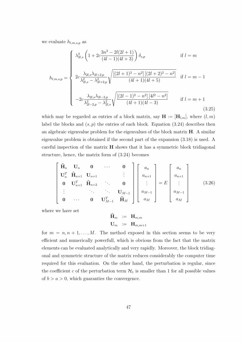
we evaluate hl,m,s,p as
hl,m,s,p =
λ22l,s
(1 + 2c
3n2 − 2l(2l + 1)
(4l − 1)(4l + 3)
)δs,p if l = m
2cλ2l,sλ2l+2,p
λ22l,s − λ2
2l+2,p
√[(2l + 1)2 − n2] [(2l + 2)2 − n2]
(4l + 1)(4l + 5)if l = m− 1
−2cλ2l,sλ2l−2,p
λ22l−2,p − λ2
2l,s
√[(2l − 1)2 − n2] [4l2 − n2]
(4l + 1)(4l − 3)if l = m + 1
(3.25)
which may be regarded as entries of a block matrix, say H := [Hl,m], where (l, m)
label the blocks and (s, p) the entries of each block. Equation (3.24) describes then
an algebraic eigenvalue problem for the eigenvalues of the block matrix H. A similar
eigenvalue problem is obtained if the second part of the expansion (3.18) is used. A
careful inspection of the matrix H shows that it has a symmetric block tridiagonal
structure, hence, the matrix form of (3.24) becomes
Hn Un 0 · · · 0
UTn Hn+1 Un+1
...
0 UTn+1 Hn+2
. . . 0...
. . . . . . UM−1
0 · · · 0 UTM−1 HM
an
an+1
...
aM−1
aM
= E
an
an+1
...
aM−1
aM
(3.26)
where we have setHm := Hm,m
Um := Hm,m+1
for m = n, n + 1, . . . , M . The method exposed in this section seems to be very
efficient and numerically powerfull, which is obvious from the fact that the matrix
elements can be evaluated analytically and very rapidly. Moreover, the block tridiag-
onal and symmetric structure of the matrix reduces considerably the computer time
required for this evaluation. On the other hand, the perturbation is regular, since
the coefficient c of the perturbation term H1 is smaller than 1 for all possible values
of b > a > 0, which guaranties the convergence.
47
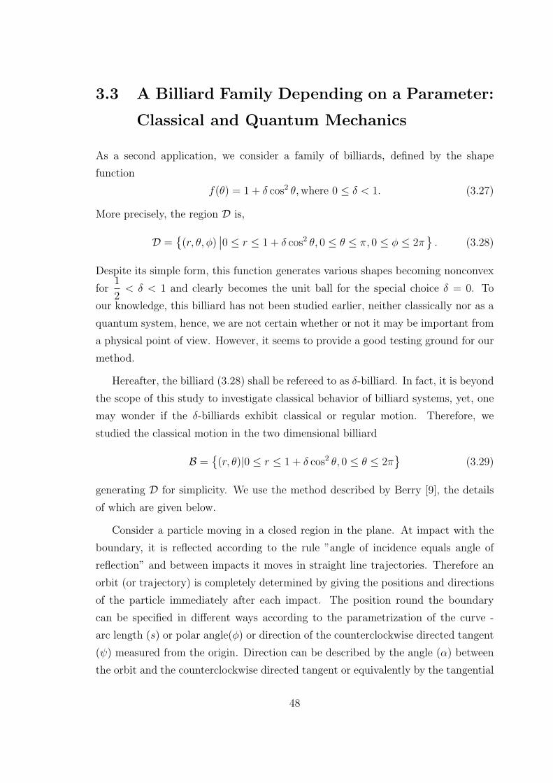
3.3 A Billiard Family Depending on a Parameter:
Classical and Quantum Mechanics
As a second application, we consider a family of billiards, defined by the shape
function
f(θ) = 1 + δ cos2 θ, where 0 ≤ δ < 1. (3.27)
More precisely, the region D is,
D ={(r, θ, φ)
∣∣0 ≤ r ≤ 1 + δ cos2 θ, 0 ≤ θ ≤ π, 0 ≤ φ ≤ 2π}
. (3.28)
Despite its simple form, this function generates various shapes becoming nonconvex
for1
2< δ < 1 and clearly becomes the unit ball for the special choice δ = 0. To
our knowledge, this billiard has not been studied earlier, neither classically nor as a
quantum system, hence, we are not certain whether or not it may be important from
a physical point of view. However, it seems to provide a good testing ground for our
method.
Hereafter, the billiard (3.28) shall be refereed to as δ-billiard. In fact, it is beyond
the scope of this study to investigate classical behavior of billiard systems, yet, one
may wonder if the δ-billiards exhibit classical or regular motion. Therefore, we
studied the classical motion in the two dimensional billiard
B ={(r, θ)|0 ≤ r ≤ 1 + δ cos2 θ, 0 ≤ θ ≤ 2π
}(3.29)
generating D for simplicity. We use the method described by Berry [9], the details
of which are given below.
Consider a particle moving in a closed region in the plane. At impact with the
boundary, it is reflected according to the rule ”angle of incidence equals angle of
reflection” and between impacts it moves in straight line trajectories. Therefore an
orbit (or trajectory) is completely determined by giving the positions and directions
of the particle immediately after each impact. The position round the boundary
can be specified in different ways according to the parametrization of the curve -
arc length (s) or polar angle(φ) or direction of the counterclockwise directed tangent
(ψ) measured from the origin. Direction can be described by the angle (α) between
the orbit and the counterclockwise directed tangent or equivalently by the tangential
48
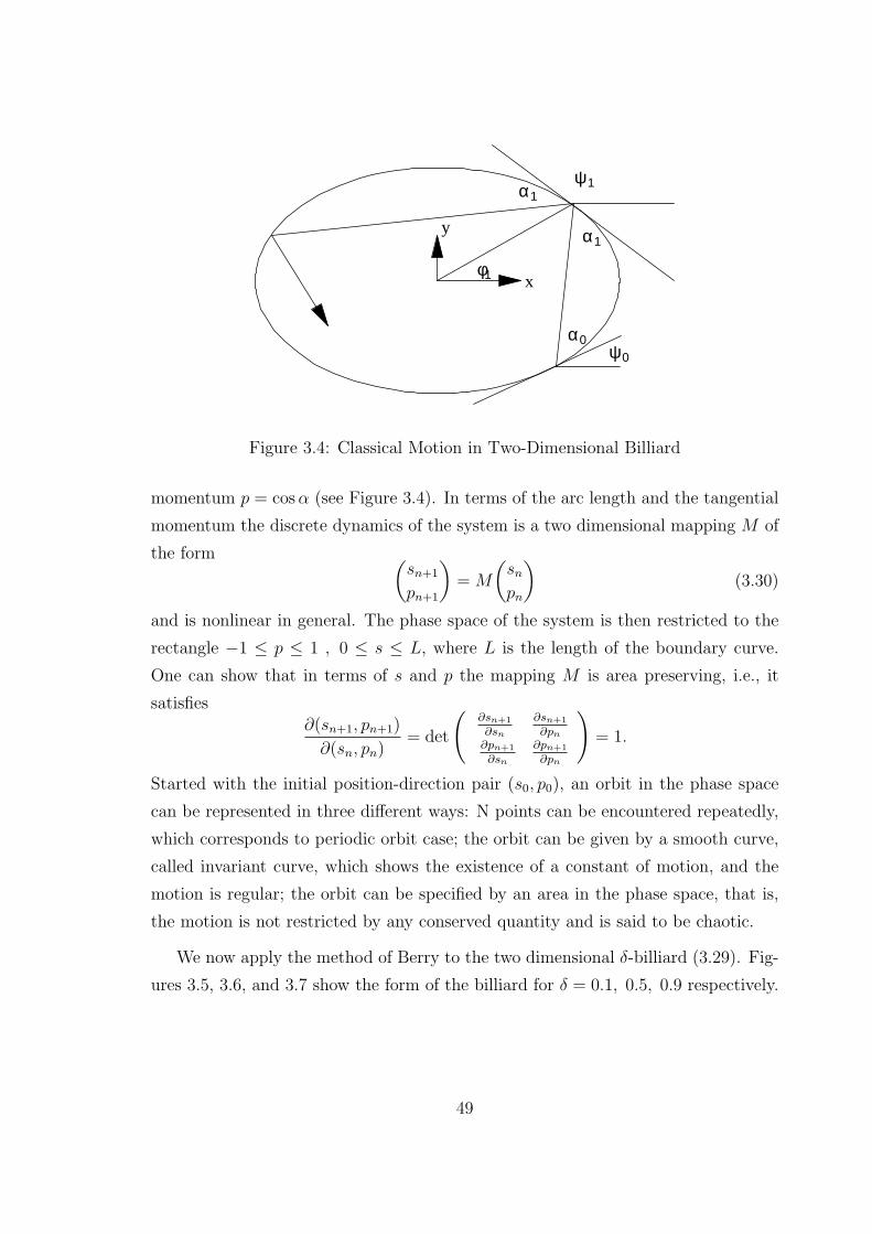
α1
α1ψ1
xφ1
y
ψ0
α0
Figure 3.4: Classical Motion in Two-Dimensional Billiard
momentum p = cos α (see Figure 3.4). In terms of the arc length and the tangential
momentum the discrete dynamics of the system is a two dimensional mapping M of
the form (sn+1
pn+1
)= M
(sn
pn
)(3.30)
and is nonlinear in general. The phase space of the system is then restricted to the
rectangle −1 ≤ p ≤ 1 , 0 ≤ s ≤ L, where L is the length of the boundary curve.
One can show that in terms of s and p the mapping M is area preserving, i.e., it
satisfies∂(sn+1, pn+1)
∂(sn, pn)= det
(∂sn+1
∂sn
∂sn+1
∂pn
∂pn+1
∂sn
∂pn+1
∂pn
)= 1.
Started with the initial position-direction pair (s0, p0), an orbit in the phase space
can be represented in three different ways: N points can be encountered repeatedly,
which corresponds to periodic orbit case; the orbit can be given by a smooth curve,
called invariant curve, which shows the existence of a constant of motion, and the
motion is regular; the orbit can be specified by an area in the phase space, that is,
the motion is not restricted by any conserved quantity and is said to be chaotic.
We now apply the method of Berry to the two dimensional δ-billiard (3.29). Fig-
ures 3.5, 3.6, and 3.7 show the form of the billiard for δ = 0.1, 0.5, 0.9 respectively.
49
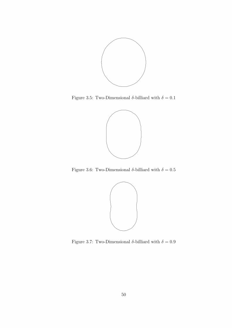
Figure 3.5: Two-Dimensional δ-billiard with δ = 0.1
Figure 3.6: Two-Dimensional δ-billiard with δ = 0.5
Figure 3.7: Two-Dimensional δ-billiard with δ = 0.9
50
The billiard mapping M can be constructed by means of the following relations
between the arc length s of the curve measured from the origin, the turning angle ψ
(angle between the forward tangent and the positive x-axis), the polar angle φ and
the angle α between forward tangent and the orbit. Observe that as a function of
the polar angle φ, the boundary curve can be written as r = 1+δ sin2 φ, so that then
the arc length s can be computed from
s =
∫ φ
0
[(r′(t))2 + r2(t)
]1/2dt.
On the other hand, the relation between the turning angle and the arc length is
known to be
ψ =π
2+
∫ φ
0
κ(t)[(r′(t))2 + r2(t)
]1/2dt
where κ(t) is the local curvature. It can be seen from Figure 3.4 that the slope
of the trajectory between two bounces isy(φ1)− y(φ0)
x(φ1)− x(φ0)and is also expressible as
tan(ψ0 + α0). Since
x(φ) = r(φ) cos φ = (1 + δ sin2 φ) cos φ
y(φ) = r(φ) sin φ = (1 + δ sin2 φ) sin φ
we obtainr(φ1) sin φ1 − r(φ0) sin φ0
r(φ1) cos φ1 − r(φ0) cos φ0
=sin(ψ0 + α0)
cos(ψ0 + α0).
This relation can be simplified as
r(φ1) sin(φ1 − ψ0 − α0) = r(φ0) sin(φ0 − ψ0 − α0)
Figure 3.4 shows that the slope of the orbit through two consecutive bounces can be
also given by tan(ψ1 − α1). Hence, we have
tan(ψ0 + α0) = tan(ψ1 − α1).
We express the curvature
κ(φ) =|2(r′(φ))2 + r2(φ)− r(φ)r′′(φ)|
((r′(φ))2 + r2(φ))3/2
of the boundary curve as a function of the polar angle and employ these relations to
construct the following algorithm for computing successive bounces.
51
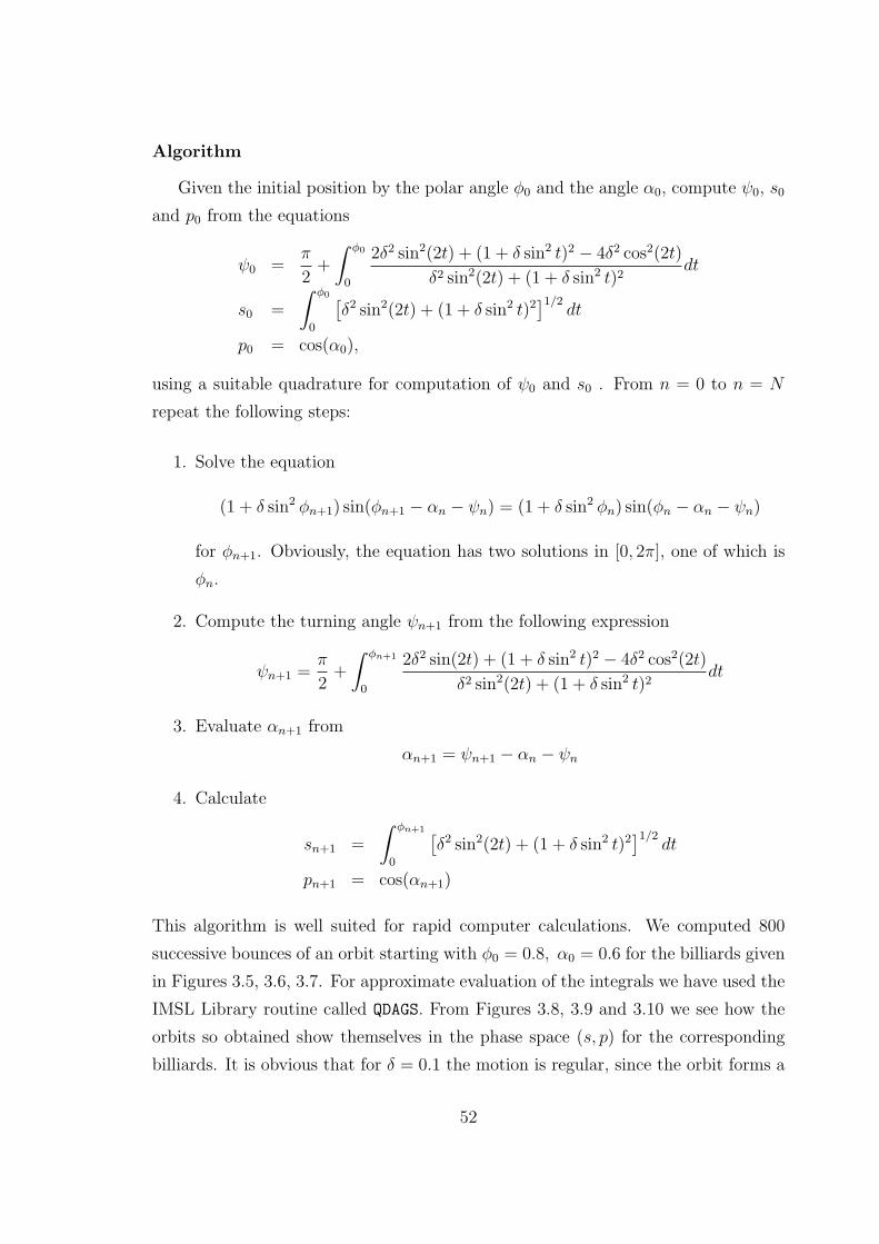
Algorithm
Given the initial position by the polar angle φ0 and the angle α0, compute ψ0, s0
and p0 from the equations
ψ0 =π
2+
∫ φ0
0
2δ2 sin2(2t) + (1 + δ sin2 t)2 − 4δ2 cos2(2t)
δ2 sin2(2t) + (1 + δ sin2 t)2dt
s0 =
∫ φ0
0
[δ2 sin2(2t) + (1 + δ sin2 t)2
]1/2dt
p0 = cos(α0),
using a suitable quadrature for computation of ψ0 and s0 . From n = 0 to n = N
repeat the following steps:
1. Solve the equation
(1 + δ sin2 φn+1) sin(φn+1 − αn − ψn) = (1 + δ sin2 φn) sin(φn − αn − ψn)
for φn+1. Obviously, the equation has two solutions in [0, 2π], one of which is
φn.
2. Compute the turning angle ψn+1 from the following expression
ψn+1 =π
2+
∫ φn+1
0
2δ2 sin(2t) + (1 + δ sin2 t)2 − 4δ2 cos2(2t)
δ2 sin2(2t) + (1 + δ sin2 t)2dt
3. Evaluate αn+1 from
αn+1 = ψn+1 − αn − ψn
4. Calculate
sn+1 =
∫ φn+1
0
[δ2 sin2(2t) + (1 + δ sin2 t)2
]1/2dt
pn+1 = cos(αn+1)
This algorithm is well suited for rapid computer calculations. We computed 800
successive bounces of an orbit starting with φ0 = 0.8, α0 = 0.6 for the billiards given
in Figures 3.5, 3.6, 3.7. For approximate evaluation of the integrals we have used the
IMSL Library routine called QDAGS. From Figures 3.8, 3.9 and 3.10 we see how the
orbits so obtained show themselves in the phase space (s, p) for the corresponding
billiards. It is obvious that for δ = 0.1 the motion is regular, since the orbit forms a
52
curve in the phase space, for δ = 0.5 and δ = 0.9 the orbit is represented by an area
which indicates the presence of a chaotic motion.
Next, consider the three-dimensional quantum δ-billiards (3.28) for the same
values of the parameter δ, i.e., δ = 0.1, 0.5, 0.9 (see Figures 3.11,3.12,3.13). The
shape function in terms of the transformed variable η, becomes simply
F (η) = 1 + δη2 (3.31)
so that the truncated shape function G(η) is exactly F (η). The derivatives of F (η)
can be easily computed and the entries of the coefficient matrices read as,
ani,j = γ
(n)i+n−1,j+n−1,0 + 2δ(1 + 2δ)γ
(n)i+n−1,j+n−1,2 − 3δγ
(n)i+n−1,j+n−1,4
bni,j = 2(1− δ)γ
(n)i+n−1,j+n−1,0 + 2δ(5− 3δ)γ
(n)i+n−1,j+n−1,2
−4(j + n− 1)(j + n)δ[γ
(n)i+n−1,j+n−1,2 + δγ
(n)i+n−1,j+n−1,4
]
+4jδ[γ
(n)i+n−1,j+n,1 + δγ
(n)i+n−1,j+n,3
]
cni,j = (j + n− 1)(j + n)
[γ
(n)i+n−1,j+n−1,0 + 2δγ
(n)i+n−1,j+n−1,2 + δ2γ
(n)i+n−1,j+n−1,4
]
dni,j = γ
(n)i+n−1,j+n−1,0 + 4δγ
(n)i+n−1,j+n−1,2 + 6δ2γ
(n)i+n−1,j+n−1,4
+4δ3γ(ni+n−1,j+n−1,6 + δ4γ
(n)i+n−1,j+n−1,8.
(3.32)
The three dimensional δ-billiard is also symmetric with respect to the xy-plane,
equivalently, with respect to η = 0, therefore, eigenvalues corresponding to even and
odd eigenfunctions in η must be calculated separately. We have obtained 6 particular
spectra, namely, eigenvalues related to the even and odd eigenfunctions in η, for δ-
billiards with δ = 0.1, 0.5, and 0.9. We have also plotted the Nearest Neighbor
Spacing Histograms for these eigenvalue sets and observed good agreement with the
theoretical models. The results and a detailed discussion can be found in Chapter 4.
53
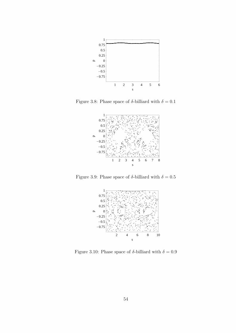
1 2 3 4 5 6s
-0.75
-0.5
-0.25
0
0.25
0.5
0.75
1
p
Figure 3.8: Phase space of δ-billiard with δ = 0.1
1 2 3 4 5 6 7 8s
-0.75
-0.5
-0.25
0
0.25
0.5
0.75
1
p
Figure 3.9: Phase space of δ-billiard with δ = 0.5
2 4 6 8 10s
-0.75
-0.5
-0.25
0
0.25
0.5
0.75
1
p
Figure 3.10: Phase space of δ-billiard with δ = 0.9
54
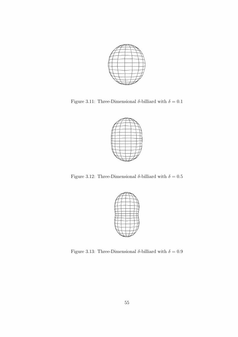
Figure 3.11: Three-Dimensional δ-billiard with δ = 0.1
Figure 3.12: Three-Dimensional δ-billiard with δ = 0.5
Figure 3.13: Three-Dimensional δ-billiard with δ = 0.9
55
Chapter 4
Numerical Results and
Discussion
In this chapter we present the results and discuss in detail the numerical methods,
algorithms and computer softwares necessary to perform the numerical implementa-
tions.
4.1 Numerical Results for the Prolate Spheroidal
Billiard
The results related to the first example introduced in Chapter 3, namely, the prolate
spheroid are shown in this section. They include six different sets of eigenvalues.
More precisely, we consider three particular sets of values for the parameters a and
b. Each set provides two classes of spectra which have been computed using both
our method and that of Moszkowski. They can be listed as:
• 1. Eigenvalues corresponding to eigenfunctions even in η and even in φ for a
prolate spheroid with a = 1, b = 1.01 (Table 4.1).
• 2. Eigenvalues corresponding to eigenfunctions odd in η and even in φ for a
prolate spheroid with a = 1, b = 1.01 (Table 4.2).
• 3. Eigenvalues corresponding to eigenfunctions even in η and even in φ for a
prolate spheroid with a = 1, b = 1.5 (Table 4.3).
56
• 4. Eigenvalues corresponding to eigenfunctions odd in η and even in φ for a
prolate spheroid with a = 1, b = 1.5 (Table 4.4).
• 5. Eigenvalues corresponding to eigenfunctions even in η and even in φ for a
prolate spheroid with a = 1, b = 2 (Table 4.5).
• 6. Eigenvalues corresponding to eigenfunctions odd in η and even in φ for a
prolate spheroid with a = 1, b = 2 (Table 4.6).
We have employed two different types of software, namely, Fortran and Math-
ematica [61]. The method of Moszkowski needs the zeros of the spherical Bessel
functions which have been computed using the Mathematica package BesselZeros
and stored in a data file. This data is required to evaluate the entries of the sym-
metric matrix H given in (3.26). A Fortran program performs this evaluation within
a desired precision and then calls two EISPACK routines to find the eigenvalues of
the matrix. The first routine, called TRED2 reduces H to a tridiagonal form, and
the second one, called TQL2 computes the eigenvalues of the resulting matrix. We
have observed that the method is very efficient in the sense of computing time and
numerical performance.
The numerical implementation of our method is much more complicated. In order
to follow up the procedure and reduce the size of the memory, we executed each step
of the method in an individual computer program. First, a Fortran program evaluates
and stores the coefficients γ(n)i,j,k. A second Fortran program computes and stores the
coefficient matrices An, Bn, Cn and Dn. Then this data is used in a Mathematica
program which performs the Cholesky decomposition of An and consequently gives
the matrices Qn, Rn and Tn, the numbers µni , the orders νn
i of the Bessel functions
and their zeros λi,s. Another Fortran program evaluates the integrals I(ρ, µ, a, σ, b)
and the matrices H and W. The last Fortran program calls the EISPACK routine
QZIT, based on the QZ-factorization method for computation of the eigenvalues of
the generalized eigenvalue problem
Hx = EWx. (4.1)
Truncation orders of the shape function have been taken as K = 8, K = 16
and K = 20 for the cases a = 1, b = 1.01, a = 1, b = 1.5 and a = 1, b = 2
57
respectively. This choice has been done after checking the precision of the eigenvalues
obtained by taking two consecutive values of K. To be specific, we have observed
that the significant digits in the computed eigenvalues do not increase by taking
K = 9 in the first case, K = 17 in the second, and K = 21 in the last case.
Thus, for each particular prolate spheroid, we obtained the eigenvalues corresponding
eigenfunctions even and odd in η. Hereafter they shall be refereed to as “even” and
“odd” eigenvalues for brevity. Truncation order M has been taken as 16 for each case
and both the methods, while the truncation order P varies in accordance with M .
Thus, we have solved the problem (4.1) 16 times. More specifically, we have taken
n = 0 and P = 20; n = 1 and P = 19, . . ., n = 16 and P = 4. On the other hand,
we have determined a minimum precision requirement, which has been achieved for
all eigenvalues in the following ranges:
• a = 1, b = 1.01 even eigenvalues in the range 0 − 375; odd eigenvalues in the
range 0− 375
• a = 1, b = 1.5 even eigenvalues in the range 0 − 220; odd eigenvalues in the
range 0− 220
• a = 1, b = 2 even eigenvalues in the range 0−155; odd eigenvalues in the range
0− 155.
Thus, we have observed that it actually suffices to take n = 12, since for larger
values of n the resulting eigenvalues are out of the given ranges. The convergence
rates have been routinely checked one more time, by comparing the results obtained
for two consecutive values of the truncation order M . The tables clearly show that
the accuracy is 7 digits in the case a = 1, b = 1.01, 4 digits in the case a = 1,
b = 1.5 and 3 digits for a = 1, b = 2. The poor convergence in the last case is a
consequence of the “large” value of β = 0.75. In this last example, the significance
of the choice of the shape function clearly shows itself. In fact, the truncation order
K = 20 implies |F (η)−G(η)| ≈ 10−4, i.e., this is a “bad” approximation. On the
other hand, increase of K yields other problems, like large memory requirements.
Furthermore, recalling that the shape function F (η) has been defined as
F (η) = 1 +∞∑
k=1
αkηk
58
it is also worth mentioning here that it is necessary to have∑∞
k=1 αkηk < 1 in
order that the perturbation is regular. For this reason, we have not treated prolate
spheroids with larger values of β. However, in the study of billiard systems the shape
of the billiard is of importance but not its volume, therefore, this additional condition
on the shape function does not restrict the variety of the billiards too much.
The most “expensive” part of the algorithm is the approximate calculation of the
integrals
I(ρ, ν, σ, α, β) =
∫ 1
0
ξρJν(αξ)Jσ(βξ)dξ
and in fact, it takes nearly the whole computing time. We have used the formula [31]
∫ 1
0
ξρJν(αξ)Jσ(βξ)dξ =ανβσ
2ν+σΓ(ν + 1)Γ(σ + 1)×
∞∑i=0
(−1)i(α/2)2i2F1(−i,−ν + i; σ + 1; β2
α2 )
i!(ρ + ν + σ + 2i + 1)(ν + 1)i
(4.2)
where 2F1 denotes the Hypergeometric function and (ν + 1)i the Pochammer’s sym-
bol. The series has been proven to be convergent for β/α < 1. However, for large
values of α and β the convergence is very slow, so that, the formula (4.2) is meaning-
less. Moreover, the convergence rate of the series cannot be improved by means of
some known methods. Therefore, for large α and β, a suitable quadrature seems to
be more appropriate. One can then take advantage of some standard routines avail-
able elsewhere to evaluate the Bessel functions for small variables and asymptotic
expansions for large variables [59]. For the eigenvalue ranges considered in this work,
relatively small values of α and β have been needed, so, we have applied the formula
(4.2), yet, even in this case we have performed a suitable scaling on the terms of the
series to get better results.
Next, we give the tabulated eigenvalues. In all the tables E(1) denotes eigenvalues
obtained using our method, and E(2) denotes eigenvalues obtained using the method
of Moszkowski.
59
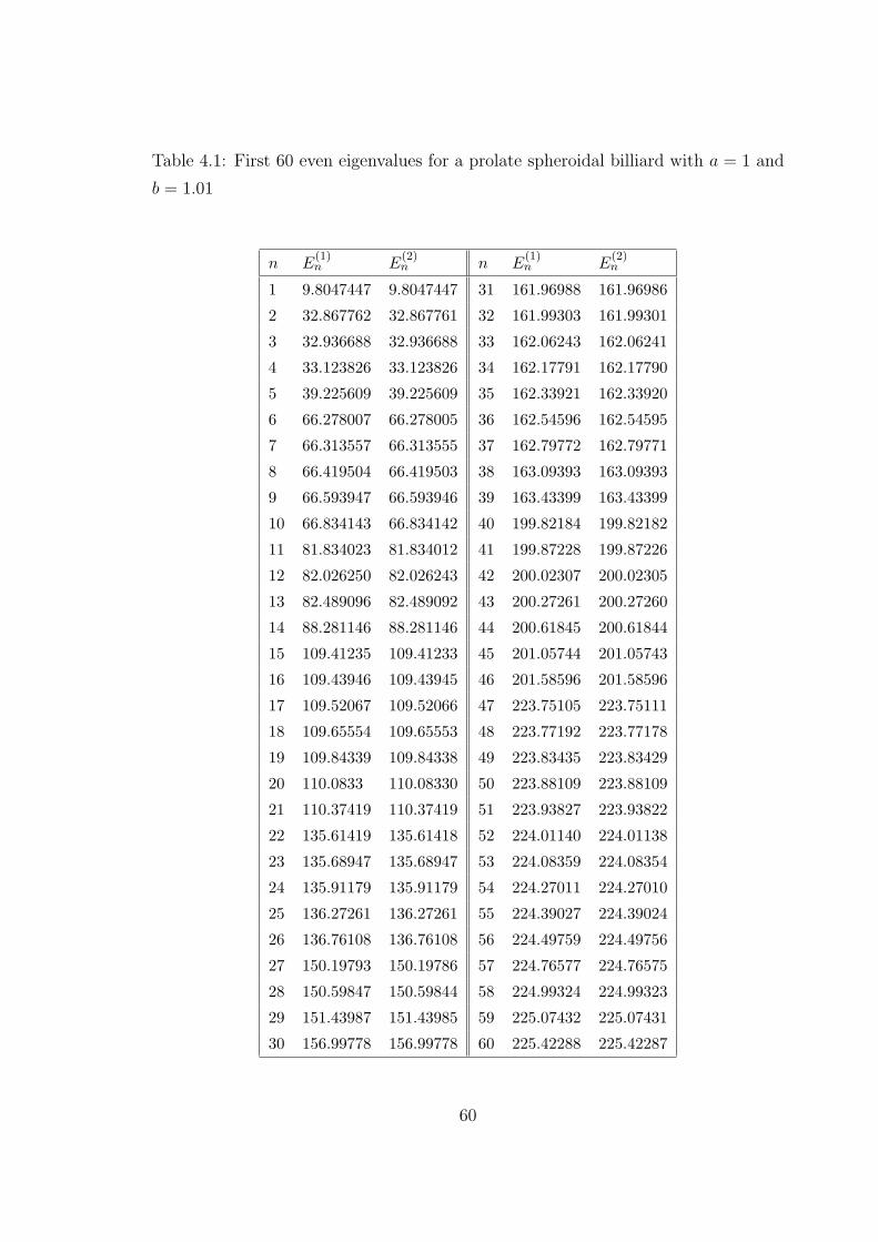
Table 4.1: First 60 even eigenvalues for a prolate spheroidal billiard with a = 1 and
b = 1.01
n E(1)n E
(2)n n E
(1)n E
(2)n
1 9.8047447 9.8047447 31 161.96988 161.96986
2 32.867762 32.867761 32 161.99303 161.99301
3 32.936688 32.936688 33 162.06243 162.06241
4 33.123826 33.123826 34 162.17791 162.17790
5 39.225609 39.225609 35 162.33921 162.33920
6 66.278007 66.278005 36 162.54596 162.54595
7 66.313557 66.313555 37 162.79772 162.79771
8 66.419504 66.419503 38 163.09393 163.09393
9 66.593947 66.593946 39 163.43399 163.43399
10 66.834143 66.834142 40 199.82184 199.82182
11 81.834023 81.834012 41 199.87228 199.87226
12 82.026250 82.026243 42 200.02307 200.02305
13 82.489096 82.489092 43 200.27261 200.27260
14 88.281146 88.281146 44 200.61845 200.61844
15 109.41235 109.41233 45 201.05744 201.05743
16 109.43946 109.43945 46 201.58596 201.58596
17 109.52067 109.52066 47 223.75105 223.75111
18 109.65554 109.65553 48 223.77192 223.77178
19 109.84339 109.84338 49 223.83435 223.83429
20 110.0833 110.08330 50 223.88109 223.88109
21 110.37419 110.37419 51 223.93827 223.93822
22 135.61419 135.61418 52 224.01140 224.01138
23 135.68947 135.68947 53 224.08359 224.08354
24 135.91179 135.91179 54 224.27011 224.27010
25 136.27261 136.27261 55 224.39027 224.39024
26 136.76108 136.76108 56 224.49759 224.49756
27 150.19793 150.19786 57 224.76577 224.76575
28 150.59847 150.59844 58 224.99324 224.99323
29 151.43987 151.43985 59 225.07432 225.07431
30 156.99778 156.99778 60 225.42288 225.42287
60
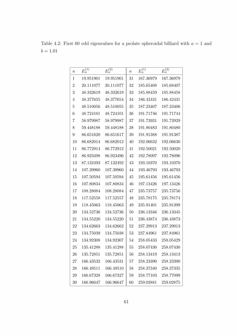
Table 4.2: First 60 odd eigenvalues for a prolate spheroidal billiard with a = 1 and
b = 1.01
n E(1)n E
(2)n n E
(1)n E
(2)n
1 19.951901 19.951901 31 167.36979 167.36979
2 20.111077 20.111077 32 185.65408 185.68407
3 48.332619 48.332619 33 185.88459 185.88458
4 48.377655 48.377654 34 186.42431 186.42431
5 48.510056 48.510055 35 187.23407 187.23406
6 48.724101 48.724101 36 191.71746 191.71744
7 58.979987 58.979987 37 191.73931 191.73929
8 59.448188 59.448188 38 191.80483 191.80480
9 86.651620 86.651617 39 191.91388 191.91387
10 86.682014 86.682012 40 192.06632 192.06630
11 86.772914 86.772912 41 192.50021 192.50020
12 86.923498 86.923496 42 192.78097 192.78096
13 87.132493 87.132492 43 193.10370 193.10370
14 107.39960 107.39960 44 193.46793 193.46793
15 107.50594 107.50594 45 195.61456 195.61456
16 107.80834 107.80834 46 197.13426 197.13426
17 108.28084 108.28084 47 235.73757 235.73756
18 117.52558 117.52557 48 235.78175 235.78174
19 118.45063 118.45063 49 235.91401 235.91399
20 134.52736 134.52736 50 236.13346 236.13345
21 134.55220 134.55220 51 236.43874 236.43873
22 134.62663 134.62662 52 237.29913 237.29913
23 134.75039 134.75038 53 237.84961 237.84961
24 134.92308 134.92307 54 258.05433 258.05429
25 135.41288 135.41288 55 258.07430 258.07430
26 135.72851 135.72851 56 258.13419 258.13413
27 166.43532 166.43531 57 258.23390 258.23390
28 166.49511 166.49510 58 258.37340 258.37335
29 166.67328 166.67327 59 258.77103 258.77099
30 166.96647 166.96647 60 259.02881 259.02875
61
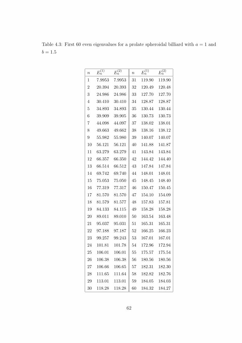
Table 4.3: First 60 even eigenvalues for a prolate spheroidal billiard with a = 1 and
b = 1.5
n E(1)n E
(2)n n E
(1)n E
(2)n
1 7.9953 7.9953 31 119.90 119.90
2 20.394 20.393 32 120.49 120.48
3 24.986 24.986 33 127.70 127.70
4 30.410 30.410 34 128.87 128.87
5 34.893 34.893 35 130.44 130.44
6 39.909 39.905 36 130.73 130.73
7 44.098 44.097 37 138.02 138.01
8 49.663 49.662 38 138.16 138.12
9 55.982 55.980 39 140.07 140.07
10 56.121 56.121 40 141.88 141.87
11 63.279 63.279 41 143.84 143.84
12 66.357 66.350 42 144.42 144.40
13 66.514 66.512 43 147.84 147.84
14 69.742 69.740 44 148.01 148.01
15 75.053 75.050 45 148.45 148.40
16 77.319 77.317 46 150.47 150.45
17 81.570 81.570 47 154.10 154.09
18 81.579 81.577 48 157.83 157.81
19 84.133 84.115 49 158.28 158.28
20 89.011 89.010 50 163.54 163.48
21 95.037 95.031 51 165.31 165.31
22 97.188 97.187 52 166.25 166.23
23 99.257 99.243 53 167.01 167.01
24 101.81 101.78 54 172.96 172.94
25 106.01 106.01 55 175.57 175.54
26 106.38 106.38 56 180.56 180.56
27 106.66 106.65 57 182.31 182.30
28 111.65 111.64 58 182.82 182.76
29 113.01 113.01 59 184.05 184.03
30 118.28 118.28 60 184.32 184.27
62
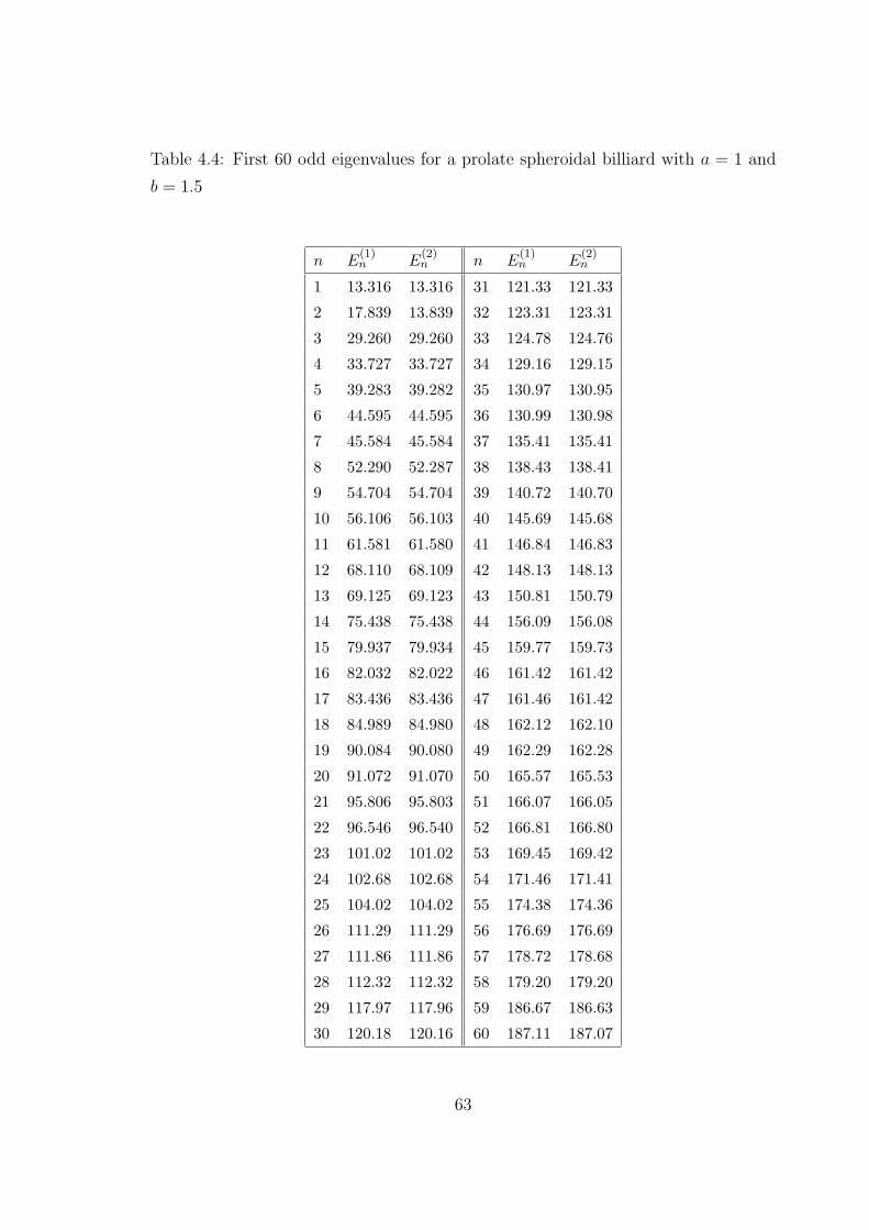
Table 4.4: First 60 odd eigenvalues for a prolate spheroidal billiard with a = 1 and
b = 1.5
n E(1)n E
(2)n n E
(1)n E
(2)n
1 13.316 13.316 31 121.33 121.33
2 17.839 13.839 32 123.31 123.31
3 29.260 29.260 33 124.78 124.76
4 33.727 33.727 34 129.16 129.15
5 39.283 39.282 35 130.97 130.95
6 44.595 44.595 36 130.99 130.98
7 45.584 45.584 37 135.41 135.41
8 52.290 52.287 38 138.43 138.41
9 54.704 54.704 39 140.72 140.70
10 56.106 56.103 40 145.69 145.68
11 61.581 61.580 41 146.84 146.83
12 68.110 68.109 42 148.13 148.13
13 69.125 69.123 43 150.81 150.79
14 75.438 75.438 44 156.09 156.08
15 79.937 79.934 45 159.77 159.73
16 82.032 82.022 46 161.42 161.42
17 83.436 83.436 47 161.46 161.42
18 84.989 84.980 48 162.12 162.10
19 90.084 90.080 49 162.29 162.28
20 91.072 91.070 50 165.57 165.53
21 95.806 95.803 51 166.07 166.05
22 96.546 96.540 52 166.81 166.80
23 101.02 101.02 53 169.45 169.42
24 102.68 102.68 54 171.46 171.41
25 104.02 104.02 55 174.38 174.36
26 111.29 111.29 56 176.69 176.69
27 111.86 111.86 57 178.72 178.68
28 112.32 112.32 58 179.20 179.20
29 117.97 117.96 59 186.67 186.63
30 120.18 120.16 60 187.11 187.07
63
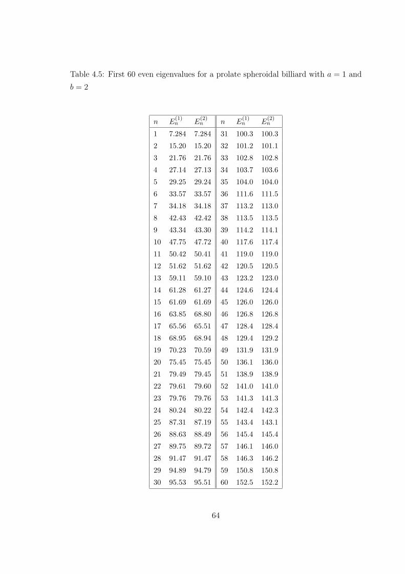
Table 4.5: First 60 even eigenvalues for a prolate spheroidal billiard with a = 1 and
b = 2
n E(1)n E
(2)n n E
(1)n E
(2)n
1 7.284 7.284 31 100.3 100.3
2 15.20 15.20 32 101.2 101.1
3 21.76 21.76 33 102.8 102.8
4 27.14 27.13 34 103.7 103.6
5 29.25 29.24 35 104.0 104.0
6 33.57 33.57 36 111.6 111.5
7 34.18 34.18 37 113.2 113.0
8 42.43 42.42 38 113.5 113.5
9 43.34 43.30 39 114.2 114.1
10 47.75 47.72 40 117.6 117.4
11 50.42 50.41 41 119.0 119.0
12 51.62 51.62 42 120.5 120.5
13 59.11 59.10 43 123.2 123.0
14 61.28 61.27 44 124.6 124.4
15 61.69 61.69 45 126.0 126.0
16 63.85 68.80 46 126.8 126.8
17 65.56 65.51 47 128.4 128.4
18 68.95 68.94 48 129.4 129.2
19 70.23 70.59 49 131.9 131.9
20 75.45 75.45 50 136.1 136.0
21 79.49 79.45 51 138.9 138.9
22 79.61 79.60 52 141.0 141.0
23 79.76 79.76 53 141.3 141.3
24 80.24 80.22 54 142.4 142.3
25 87.31 87.19 55 143.4 143.1
26 88.63 88.49 56 145.4 145.4
27 89.75 89.72 57 146.1 146.0
28 91.47 91.47 58 146.3 146.2
29 94.89 94.79 59 150.8 150.8
30 95.53 95.51 60 152.5 152.2
64
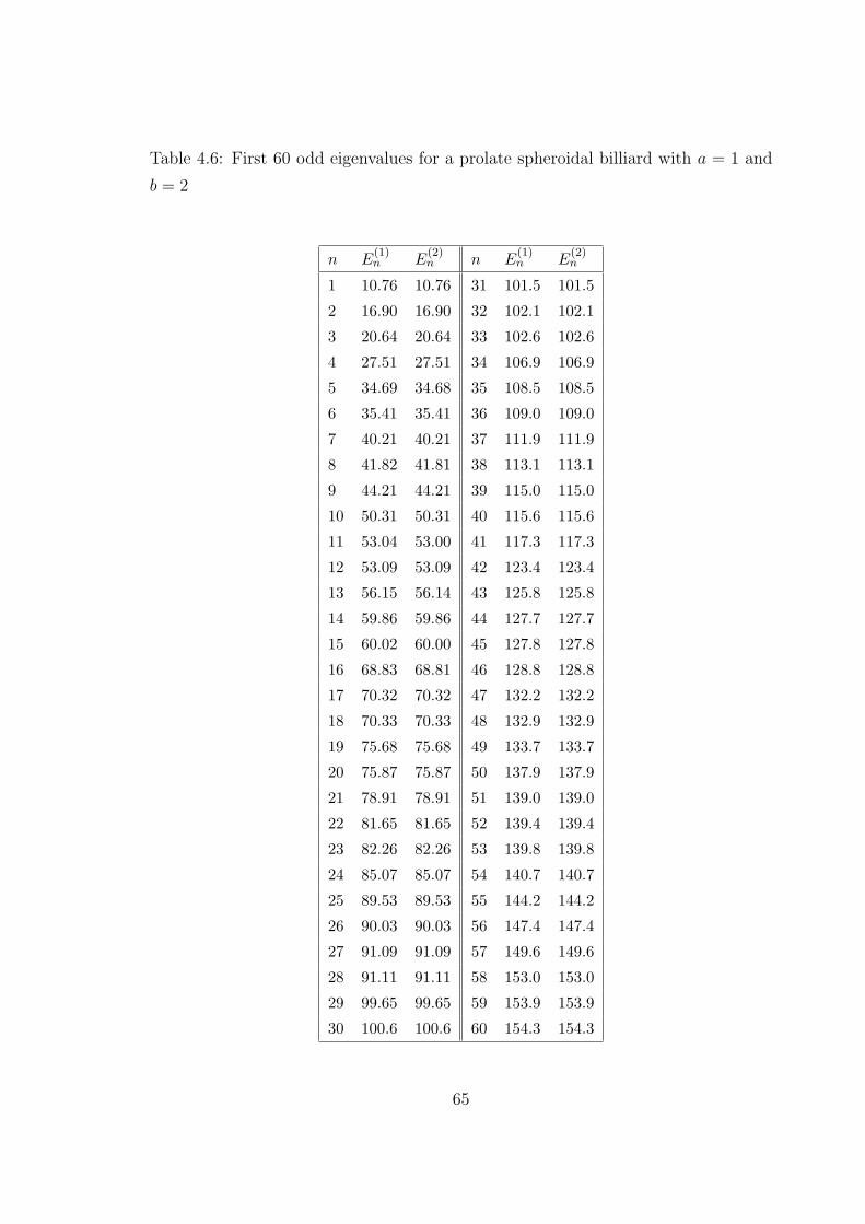
Table 4.6: First 60 odd eigenvalues for a prolate spheroidal billiard with a = 1 and
b = 2
n E(1)n E
(2)n n E
(1)n E
(2)n
1 10.76 10.76 31 101.5 101.5
2 16.90 16.90 32 102.1 102.1
3 20.64 20.64 33 102.6 102.6
4 27.51 27.51 34 106.9 106.9
5 34.69 34.68 35 108.5 108.5
6 35.41 35.41 36 109.0 109.0
7 40.21 40.21 37 111.9 111.9
8 41.82 41.81 38 113.1 113.1
9 44.21 44.21 39 115.0 115.0
10 50.31 50.31 40 115.6 115.6
11 53.04 53.00 41 117.3 117.3
12 53.09 53.09 42 123.4 123.4
13 56.15 56.14 43 125.8 125.8
14 59.86 59.86 44 127.7 127.7
15 60.02 60.00 45 127.8 127.8
16 68.83 68.81 46 128.8 128.8
17 70.32 70.32 47 132.2 132.2
18 70.33 70.33 48 132.9 132.9
19 75.68 75.68 49 133.7 133.7
20 75.87 75.87 50 137.9 137.9
21 78.91 78.91 51 139.0 139.0
22 81.65 81.65 52 139.4 139.4
23 82.26 82.26 53 139.8 139.8
24 85.07 85.07 54 140.7 140.7
25 89.53 89.53 55 144.2 144.2
26 90.03 90.03 56 147.4 147.4
27 91.09 91.09 57 149.6 149.6
28 91.11 91.11 58 153.0 153.0
29 99.65 99.65 59 153.9 153.9
30 100.6 100.6 60 154.3 154.3
65
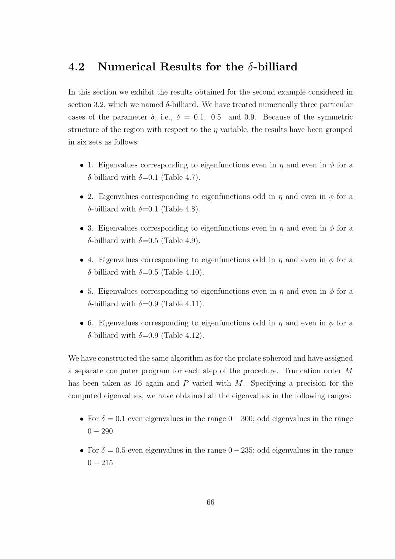
4.2 Numerical Results for the δ-billiard
In this section we exhibit the results obtained for the second example considered in
section 3.2, which we named δ-billiard. We have treated numerically three particular
cases of the parameter δ, i.e., δ = 0.1, 0.5 and 0.9. Because of the symmetric
structure of the region with respect to the η variable, the results have been grouped
in six sets as follows:
• 1. Eigenvalues corresponding to eigenfunctions even in η and even in φ for a
δ-billiard with δ=0.1 (Table 4.7).
• 2. Eigenvalues corresponding to eigenfunctions odd in η and even in φ for a
δ-billiard with δ=0.1 (Table 4.8).
• 3. Eigenvalues corresponding to eigenfunctions even in η and even in φ for a
δ-billiard with δ=0.5 (Table 4.9).
• 4. Eigenvalues corresponding to eigenfunctions odd in η and even in φ for a
δ-billiard with δ=0.5 (Table 4.10).
• 5. Eigenvalues corresponding to eigenfunctions even in η and even in φ for a
δ-billiard with δ=0.9 (Table 4.11).
• 6. Eigenvalues corresponding to eigenfunctions odd in η and even in φ for a
δ-billiard with δ=0.9 (Table 4.12).
We have constructed the same algorithm as for the prolate spheroid and have assigned
a separate computer program for each step of the procedure. Truncation order M
has been taken as 16 again and P varied with M . Specifying a precision for the
computed eigenvalues, we have obtained all the eigenvalues in the following ranges:
• For δ = 0.1 even eigenvalues in the range 0− 300; odd eigenvalues in the range
0− 290
• For δ = 0.5 even eigenvalues in the range 0− 235; odd eigenvalues in the range
0− 215
66
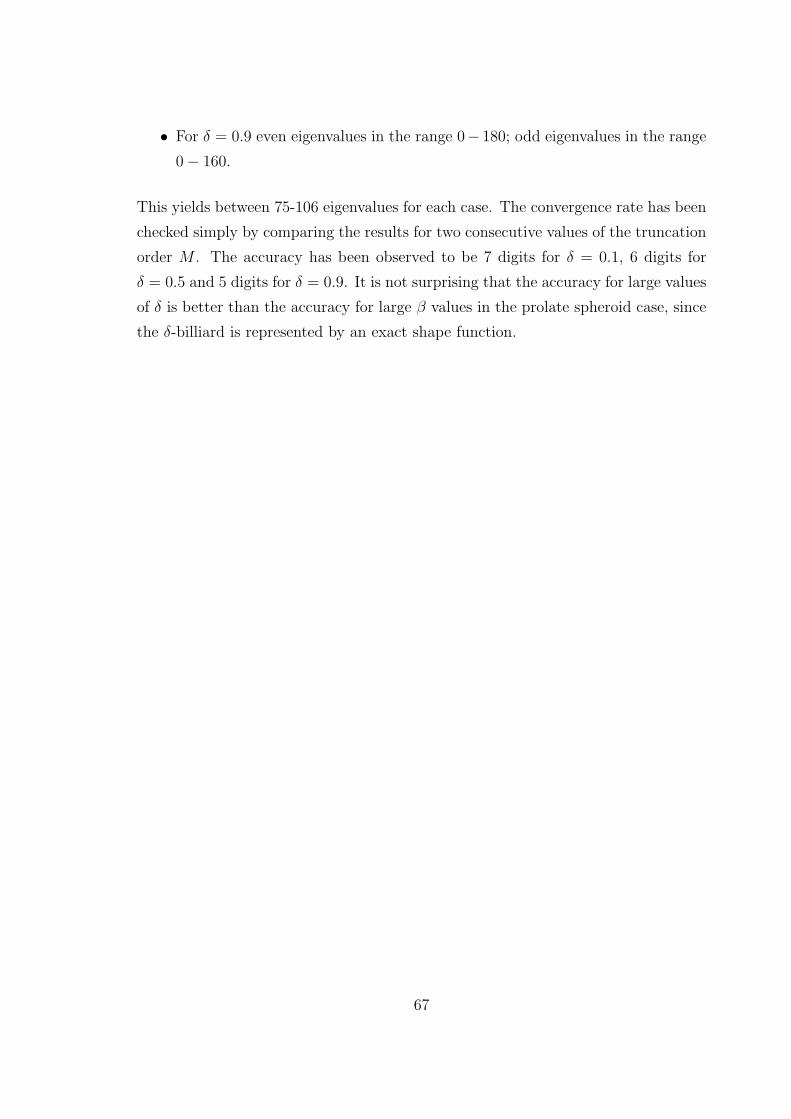
• For δ = 0.9 even eigenvalues in the range 0− 180; odd eigenvalues in the range
0− 160.
This yields between 75-106 eigenvalues for each case. The convergence rate has been
checked simply by comparing the results for two consecutive values of the truncation
order M . The accuracy has been observed to be 7 digits for δ = 0.1, 6 digits for
δ = 0.5 and 5 digits for δ = 0.9. It is not surprising that the accuracy for large values
of δ is better than the accuracy for large β values in the prolate spheroid case, since
the δ-billiard is represented by an exact shape function.
67
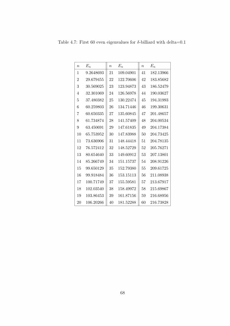
Table 4.7: First 60 even eigenvalues for δ-billiard with delta=0.1
n En n En n En
1 9.2648693 21 109.04901 41 182.13966
2 29.679455 22 122.70606 42 183.85682
3 30.569025 23 123.94873 43 186.52479
4 32.301069 24 126.56978 44 190.03627
5 37.480382 25 130.22474 45 194.31993
6 60.259803 26 134.71446 46 199.30631
7 60.650335 27 135.60845 47 201.48657
8 61.734874 28 141.57409 48 204.00534
9 63.450691 29 147.61835 49 204.17384
10 65.753952 30 147.83988 50 204.73425
11 73.636906 31 148.44418 51 204.78135
12 76.572412 32 148.52729 52 205.76271
13 80.654640 33 149.60912 53 207.13801
14 85.266749 34 151.15737 54 208.91226
15 99.650129 35 152.79380 55 209.61725
16 99.918484 36 153.15113 56 211.08938
17 100.71749 37 155.59581 57 213.67917
18 102.03540 38 158.49972 58 215.69867
19 103.86453 39 161.87156 59 216.68956
20 106.20266 40 181.52288 60 216.73828
68
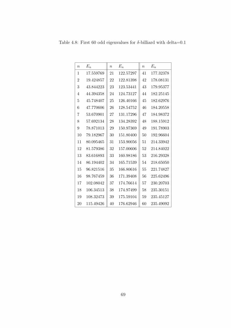
Table 4.8: First 60 odd eigenvalues for δ-billiard with delta=0.1
n En n En n En
1 17.559769 21 122.57297 41 177.32378
2 19.424857 22 122.81398 42 178.08131
3 43.844223 23 123.53441 43 179.95377
4 44.394358 24 124.73127 44 182.25145
5 45.748407 25 126.40166 45 182.62976
6 47.770606 26 128.54752 46 184.20558
7 53.670901 27 131.17296 47 184.98372
8 57.692134 28 134.28392 48 188.15912
9 78.871013 29 150.97369 49 191.78903
10 79.182967 30 151.80400 50 192.96604
11 80.095465 31 153.90056 51 214.33942
12 81.579386 32 157.00606 52 214.84022
13 83.616893 33 160.98186 53 216.29328
14 86.194402 34 165.71539 54 218.65050
15 96.821516 35 166.80616 55 221.74827
16 98.767459 36 171.39408 56 225.62496
17 102.08042 37 174.76614 57 230.20703
18 106.34513 38 174.97499 58 235.30151
19 108.32473 39 175.59104 59 235.45127
20 115.49426 40 176.62946 60 235.49092
69

Table 4.9: First 60 even eigenvalues for δ-billiard with delta=0.5
n En n En n En
1 7.63575 21 87.5637 41 138.057
2 19.9003 22 90.5275 42 138.766
3 22.8837 23 96.5736 43 139.999
4 29.1090 24 99.1163 44 140.435
5 32.6498 25 101.907 45 140.625
6 40.4220 26 102.310 46 140.900
7 42.3942 27 102.901 47 142.910
8 46.0214 28 104.310 48 146.518
9 51.0549 29 106.808 49 149.079
10 51.7918 30 109.750 50 154.247
11 59.8284 31 112.445 51 154.383
12 61.0811 32 115.087 52 155.271
13 67.7435 33 118.767 53 162.552
14 69.0006 34 119.767 54 164.716
15 71.4522 35 121.279 55 164.945
16 74.3095 36 124.331 56 168.682
17 76.0218 37 126.662 57 168.841
18 76.7052 38 127.649 58 169.138
19 80.2864 39 131.369 59 171.490
20 82.0830 40 134.833 60 174.826
70
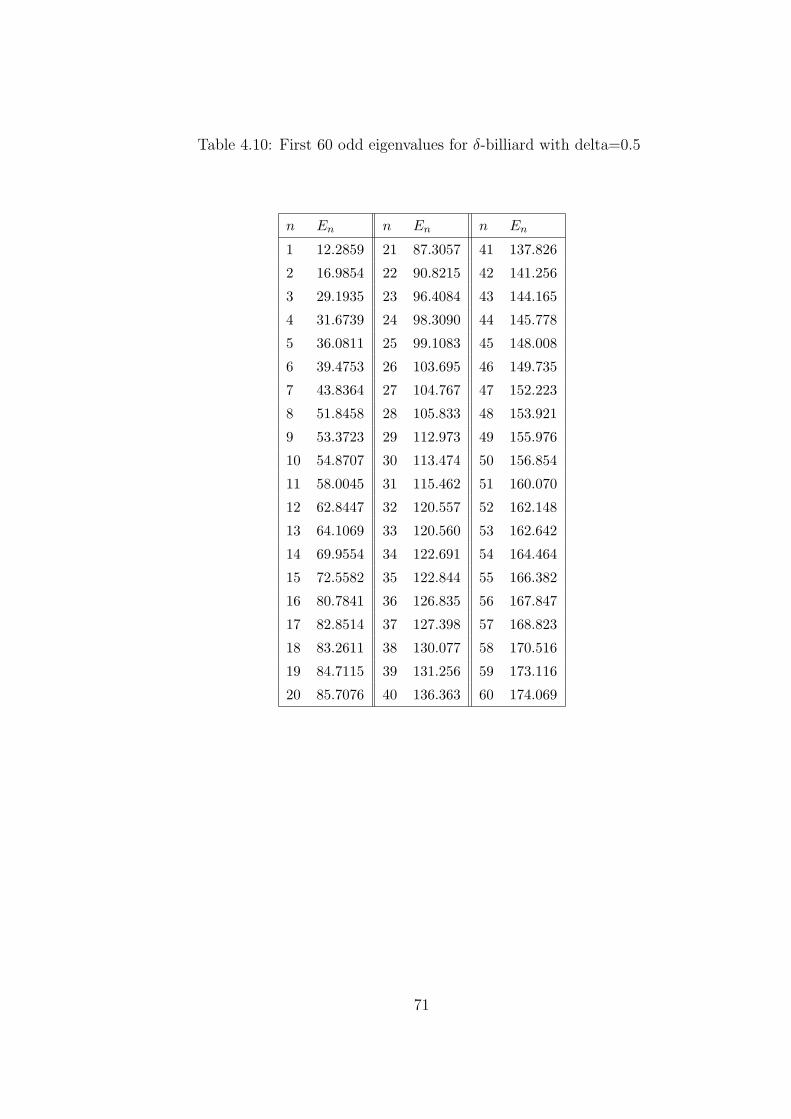
Table 4.10: First 60 odd eigenvalues for δ-billiard with delta=0.5
n En n En n En
1 12.2859 21 87.3057 41 137.826
2 16.9854 22 90.8215 42 141.256
3 29.1935 23 96.4084 43 144.165
4 31.6739 24 98.3090 44 145.778
5 36.0811 25 99.1083 45 148.008
6 39.4753 26 103.695 46 149.735
7 43.8364 27 104.767 47 152.223
8 51.8458 28 105.833 48 153.921
9 53.3723 29 112.973 49 155.976
10 54.8707 30 113.474 50 156.854
11 58.0045 31 115.462 51 160.070
12 62.8447 32 120.557 52 162.148
13 64.1069 33 120.560 53 162.642
14 69.9554 34 122.691 54 164.464
15 72.5582 35 122.844 55 166.382
16 80.7841 36 126.835 56 167.847
17 82.8514 37 127.398 57 168.823
18 83.2611 38 130.077 58 170.516
19 84.7115 39 131.256 59 173.116
20 85.7076 40 136.363 60 174.069
71
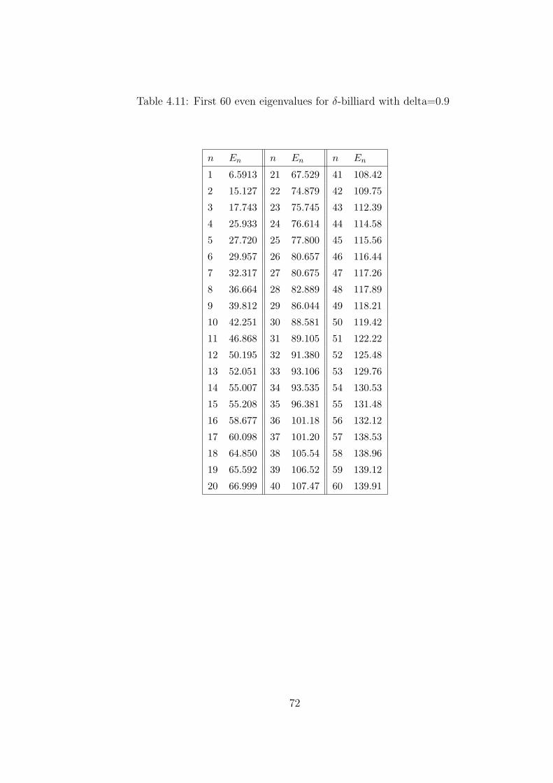
Table 4.11: First 60 even eigenvalues for δ-billiard with delta=0.9
n En n En n En
1 6.5913 21 67.529 41 108.42
2 15.127 22 74.879 42 109.75
3 17.743 23 75.745 43 112.39
4 25.933 24 76.614 44 114.58
5 27.720 25 77.800 45 115.56
6 29.957 26 80.657 46 116.44
7 32.317 27 80.675 47 117.26
8 36.664 28 82.889 48 117.89
9 39.812 29 86.044 49 118.21
10 42.251 30 88.581 50 119.42
11 46.868 31 89.105 51 122.22
12 50.195 32 91.380 52 125.48
13 52.051 33 93.106 53 129.76
14 55.007 34 93.535 54 130.53
15 55.208 35 96.381 55 131.48
16 58.677 36 101.18 56 132.12
17 60.098 37 101.20 57 138.53
18 64.850 38 105.54 58 138.96
19 65.592 39 106.52 59 139.12
20 66.999 40 107.47 60 139.91
72
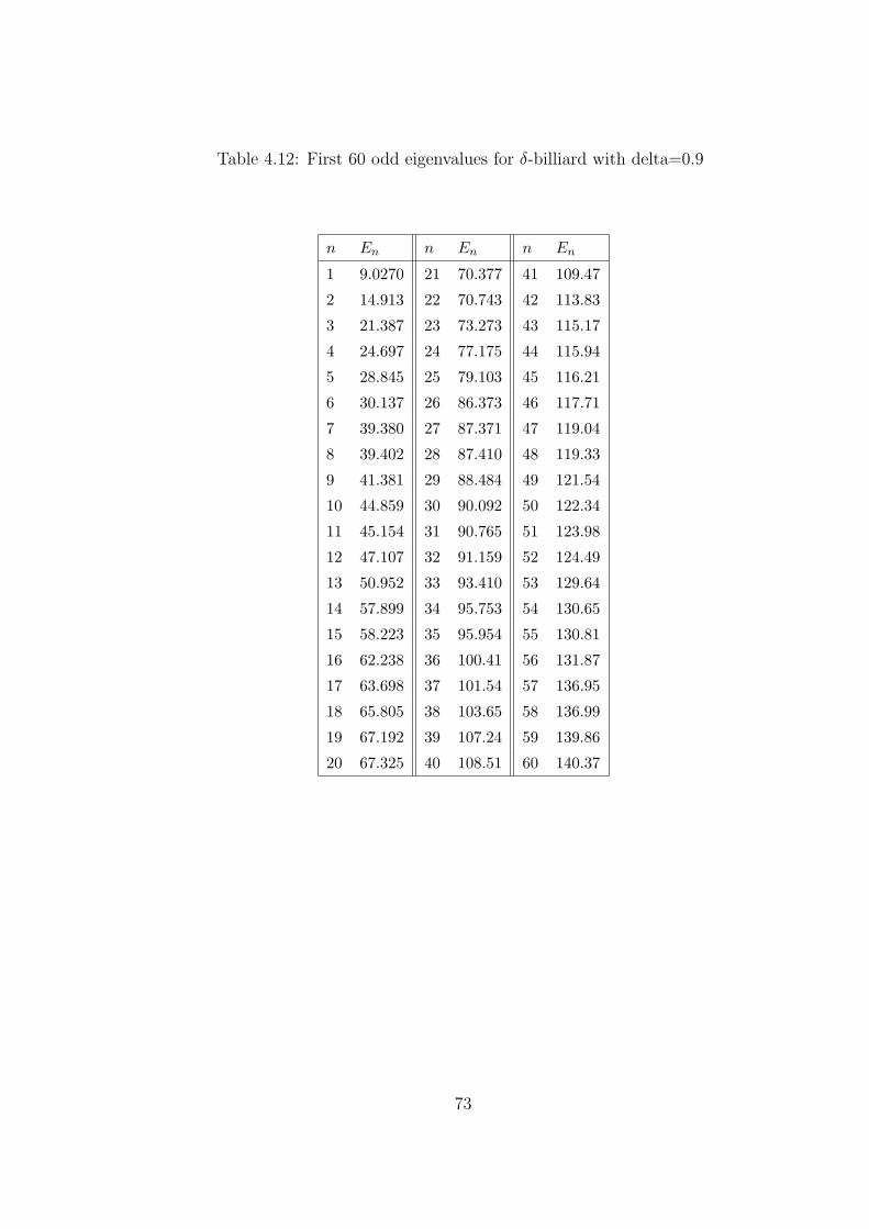
Table 4.12: First 60 odd eigenvalues for δ-billiard with delta=0.9
n En n En n En
1 9.0270 21 70.377 41 109.47
2 14.913 22 70.743 42 113.83
3 21.387 23 73.273 43 115.17
4 24.697 24 77.175 44 115.94
5 28.845 25 79.103 45 116.21
6 30.137 26 86.373 46 117.71
7 39.380 27 87.371 47 119.04
8 39.402 28 87.410 48 119.33
9 41.381 29 88.484 49 121.54
10 44.859 30 90.092 50 122.34
11 45.154 31 90.765 51 123.98
12 47.107 32 91.159 52 124.49
13 50.952 33 93.410 53 129.64
14 57.899 34 95.753 54 130.65
15 58.223 35 95.954 55 130.81
16 62.238 36 100.41 56 131.87
17 63.698 37 101.54 57 136.95
18 65.805 38 103.65 58 136.99
19 67.192 39 107.24 59 139.86
20 67.325 40 108.51 60 140.37
73
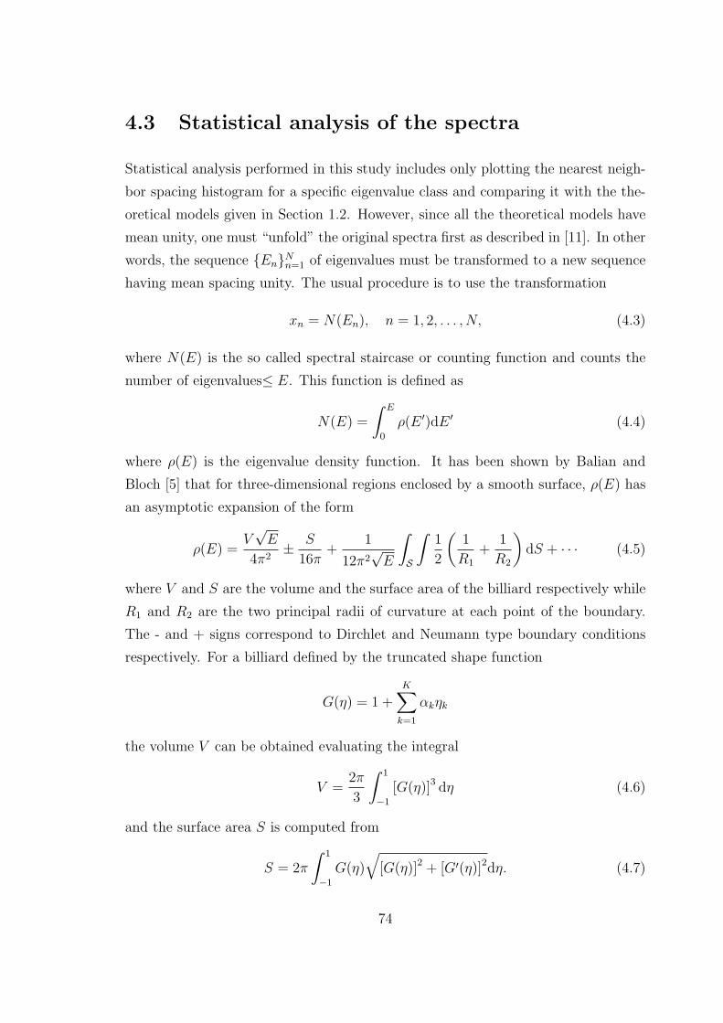
4.3 Statistical analysis of the spectra
Statistical analysis performed in this study includes only plotting the nearest neigh-
bor spacing histogram for a specific eigenvalue class and comparing it with the the-
oretical models given in Section 1.2. However, since all the theoretical models have
mean unity, one must “unfold” the original spectra first as described in [11]. In other
words, the sequence {En}Nn=1 of eigenvalues must be transformed to a new sequence
having mean spacing unity. The usual procedure is to use the transformation
xn = N(En), n = 1, 2, . . . , N, (4.3)
where N(E) is the so called spectral staircase or counting function and counts the
number of eigenvalues≤ E. This function is defined as
N(E) =
∫ E
0
ρ(E ′)dE ′ (4.4)
where ρ(E) is the eigenvalue density function. It has been shown by Balian and
Bloch [5] that for three-dimensional regions enclosed by a smooth surface, ρ(E) has
an asymptotic expansion of the form
ρ(E) =V√
E
4π2± S
16π+
1
12π2√
E
∫
S
∫1
2
(1
R1
+1
R2
)dS + · · · (4.5)
where V and S are the volume and the surface area of the billiard respectively while
R1 and R2 are the two principal radii of curvature at each point of the boundary.
The - and + signs correspond to Dirchlet and Neumann type boundary conditions
respectively. For a billiard defined by the truncated shape function
G(η) = 1 +K∑
k=1
αkηk
the volume V can be obtained evaluating the integral
V =2π
3
∫ 1
−1
[G(η)]3 dη (4.6)
and the surface area S is computed from
S = 2π
∫ 1
−1
G(η)
√[G(η)]2 + [G′(η)]2dη. (4.7)
74
The two principal radii of curvature can be obtained using the first and second
fundamental forms of the boundary surface, (see [55] for details), so that, the integral
term in (4.5) becomes
−π
{G(−1) + G(1) +
∫ 1
−1
G(η)dη
}
+π
∫ 1
−1
(1− η2){G′′(η)G(η)− [G′(η)]2
}− ηG′(η)G(η)
[G(η)]2 + [G′(η)]2dη.
(4.8)
It must be pointed out that the eigenvalue sets obtained for each case represent actu-
ally 1/4-th of the total number of eigenvalues in the corresponding interval. This is
due to the fact that we have separated the eigenfunctions according to their symme-
tries. This separation is necessary for the statistical analysis, since the degeneracies
implied by the symmetries must be avoided.
In what follows, we transformed the eigenvalue sequence {En}Nn=1 to the sequence
{xn}Nn=1 by means of the transformation
xn = N(En) =1
4
{V E
3/2n
6π2− SEn
16π+
KE1/2n
6π2
}. (4.9)
The values of V , S and K have been evaluated numerically using Mathematica. Then
we have calculated the spacing sn = xn+1 − xn and have observed that the mean
s of the sequence (sn) is s ≈ 1 in each case. Figures 4.1-4.5 show the distribution
of the sequence (sn) for each eigenvalue set computed for the δ-billiard, that is, the
so-called Nearest Neighbor Spacing (NNS) Histograms. In each Figure, the graph of
the Poisson distribution
p(s) = e−s
is plotted. In the first two figures the NNS histograms of even and odd eigenvalues
of the δ-billiard with δ=0.1 are given. The graph of the probability distribution
function of the Gaussian Orthogonal Ensemble,
p(s) =π
2se−
π4s2
is also plotted for comparison. The resemblance between the Poisson distribution
function and the histograms is remarkable for both cases. Recall that the two dimen-
sional cross-sectional billiard with δ = 0.1 exhibited regular motion. In the Figures
75
4.3 and 4.4 the NNS histograms of even and odd eigenvalues of the δ-billiard with
δ=0.5 are given. The Brody distribution
p(s) = (ν + 1)aνsν exp(−aνs
ν+1), (4.10)
where
aν =
[Γ
(ν + 2
ν + 1
)]ν+1
. (4.11)
and ν = 0.5 is also plotted and obviously, the agreement between the histogram and
the Brody model is quite good. NNS histograms for the even and odd eigenvalues of
the δ-billiard with δ = 0.9 are given in Figures 4.5 and 4.6 respectively. The graph
of Brody model with ν = 0.9 is also given for comparison. The similarity of the last
two histograms and the Brody distribution is also noticeable.
Despite the relatively small number of eigenvalues included in the histograms, we
have observed good agreement with the theoretical models. Thus, we expect that
increasing the number of the eigenvalues we will get much better statistical results.
However, the main purpose of this work is the development of the method rather
than the statistical investigation, therefore, we do not further extend our statistical
analysis.
76
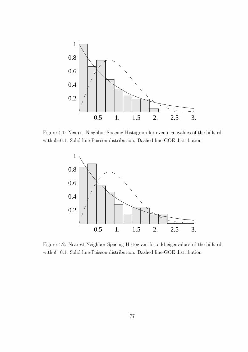
0.5 1. 1.5 2. 2.5 3.
0.2
0.4
0.6
0.8
1
Figure 4.1: Nearest-Neighbor Spacing Histogram for even eigenvalues of the billiard
with δ=0.1. Solid line-Poisson distribution. Dashed line-GOE distribution
0.5 1. 1.5 2. 2.5 3.
0.2
0.4
0.6
0.8
1
Figure 4.2: Nearest-Neighbor Spacing Histogram for odd eigenvalues of the billiard
with δ=0.1. Solid line-Poisson distribution. Dashed line-GOE distribution
77
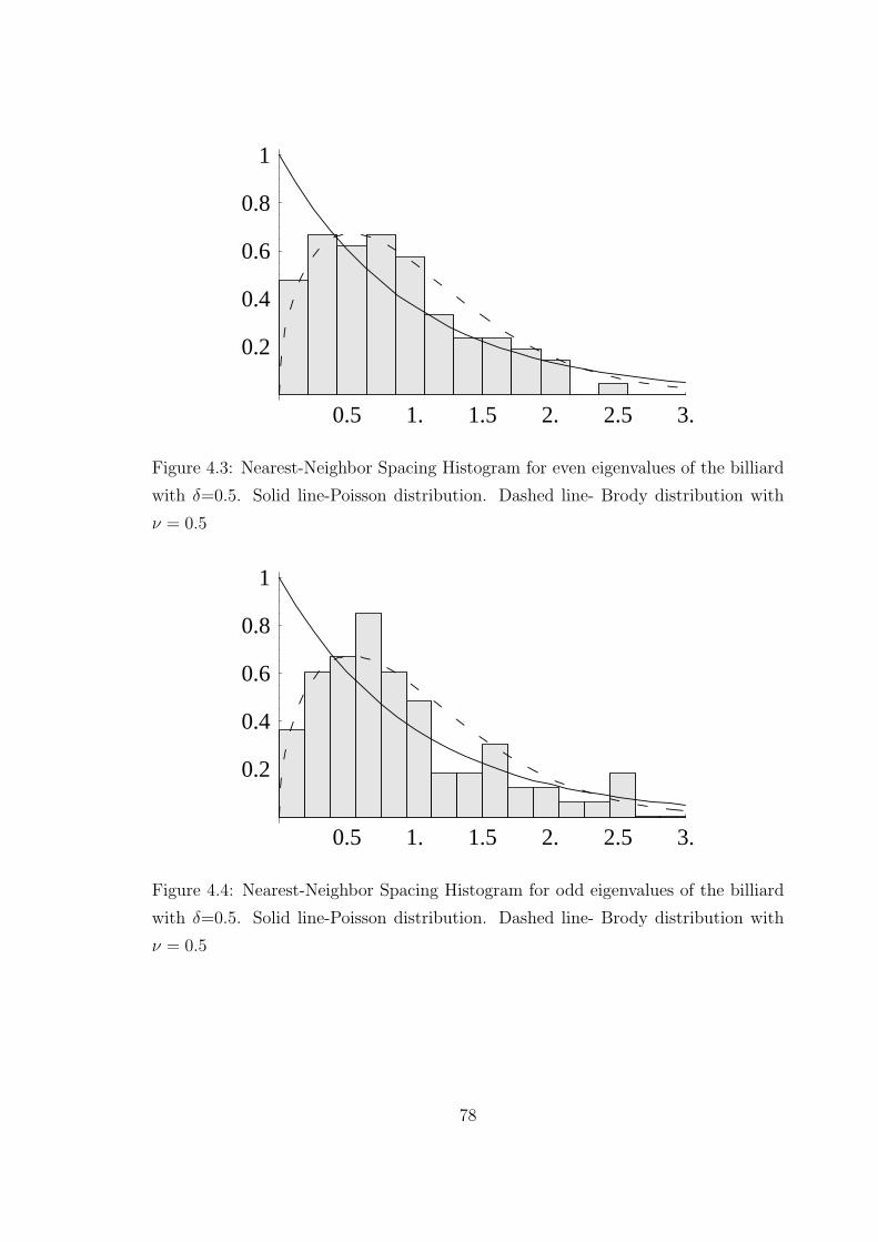
0.5 1. 1.5 2. 2.5 3.
0.2
0.4
0.6
0.8
1
Figure 4.3: Nearest-Neighbor Spacing Histogram for even eigenvalues of the billiard
with δ=0.5. Solid line-Poisson distribution. Dashed line- Brody distribution with
ν = 0.5
0.5 1. 1.5 2. 2.5 3.
0.2
0.4
0.6
0.8
1
Figure 4.4: Nearest-Neighbor Spacing Histogram for odd eigenvalues of the billiard
with δ=0.5. Solid line-Poisson distribution. Dashed line- Brody distribution with
ν = 0.5
78
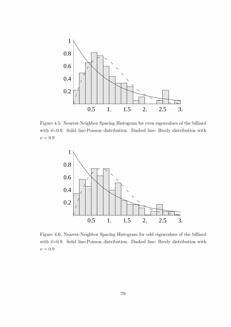
0.5 1. 1.5 2. 2.5 3.
0.2
0.4
0.6
0.8
1
Figure 4.5: Nearest-Neighbor Spacing Histogram for even eigenvalues of the billiard
with δ=0.9. Solid line-Poisson distribution. Dashed line- Brody distribution with
ν = 0.9
0.5 1. 1.5 2. 2.5 3.
0.2
0.4
0.6
0.8
1
Figure 4.6: Nearest-Neighbor Spacing Histogram for odd eigenvalues of the billiard
with δ=0.9. Solid line-Poisson distribution. Dashed line- Brody distribution with
ν = 0.9
79
Chapter 5
Conclusion
In this thesis we have presented a numerical method for computation of the eigenval-
ues of the Schrodinger equation for a particle moving freely in a closed axisymmetric
three-dimensional region. In the theory of partial differential equations, this is an
eigenvalue problem for the eigenvalues and eigenfunctions of the self-adjoint Laplace
operator subject to some additional conditions. The method employs an unusual
non-orthogonal coordinate transformation leading to an expansion in terms of Bessel
functions with real orders. Therefore, it seems to be interesting from mathematical
point of view. In fact, the expansions in Bessel functions with real orders is not
as common a tool as the expansions in terms of Bessel functions with integral or
half-an-odd integral orders.
The method is also interesting from classical and quantum mechanical points of
view, more precisely, in the study of quantum chaos, since it deals with quite gen-
eral three-dimensional billiard systems. Unlike the boundary element or collocation
methods resulting in a nonlinear problem, our method ends up with a generalized
matrix eigenvalue problem, which is more appropriate in quantum mechanics. A
similar matrix eigenvalue problem is obtained if the problem is treated with the
constraint operator method [33] for example, however, this method represents the
wavefunction of a chaotic billiard in terms of the eigenfunctions of a regular billiard.
The expansion basis of our method is closely related to the shape of the billiard,
which seems more natural.
The method has one very serious drawback. It requires computation of integrals
of products of Bessel functions of real orders, which is a very difficult numerical task.
80
In this study, computation of such integrals has been done by using a method which
is not numerically efficient, for, it is very “expensive” in the sense of computing time.
Therefore, this problem needs to be reconsidered. Moreover, for each new parameter
the integrals must be computed again. For this reason, the use of an expansion basis
of spherical Bessel functions may seem to be more appropriate. Then, it would be
sufficient to compute the integrals needed to evaluate the matrix elements once, and
use them for each new parameter. Although not reported here, we have tried such a
basis during the period of preparing the thesis. However, we have observed that the
accuracy of the eigenvalues computed in this way is less than the accuracy obtained
using the basis presented here. It must be pointed out that, despite its drawbacks,
the accuracy of our method is quite good compared with the results reported in the
literature.
The second numerical example considered in this thesis is a billiard family de-
pending on a parameter. This billiard has not been investigated before. However,
related statistical results, seem to be very interesting and we expect that they may
attract the attention of people studying chaos in classical and quantum systems.
81
References
[1] M. Abramowitz and I. A. Stegun. Handbook of Mathematical Functions. Dover,
New York, 1970.
[2] Y. Ayant and R. Arvieu. Semiclassical study of particle motion in two-
dimensional and three-dimensional elliptical boxes:i. J. Phys. A. Math. Gen.,
20:397–409, 1987.
[3] Y. Ayant and R. Arvieu. Semiclassical study of particle motion in two-
dimensional and three-dimensional elliptical boxes:ii. J. Phys. A. Math. Gen.,
20:1115–1136, 1987.
[4] A. Backer and F. Steiner. Spectral statistics in the quantized cardioid billiard.
Phys. Rev. E, 52:2463–2472, 1995.
[5] R. Balian and C. Block. Distribution of eigenfrequences for the wave function
in a finite domain i three-dimensional problem with smooth boundary surface.
Annals of Physics, 60:401–447, 1970.
[6] P. K. Banerjee. The Boundary Element Method in Engineering. McGraw-Hill,
New York, 1994.
[7] H. Bateman. Higher Transcendental Functions I. Robert E. Krieger Publishing
Company Malabar, Florida, 1953.
[8] M. V. Berry. Quantizing a classically ergodic system: Sinai‘s billiard and the
kkr method. Ann. Phys., 131:163–216, 1981.
[9] M. V. Berry. Regularity and chaos in classical mechanics, illustrated by three
deformations of a circular billiard. Eur. J. Phys., 2:91–102, 1981.
82
[10] M. V. Berry and M. Tabor. Level clustering in regular spectrum. Proc. R. Soc.
Lond. A, 356:375–395, 1977.
[11] O. Bohigas. Random matrix theories and chaotic dynamics. In M. J. Giannoni,
A. Voros, and J. Zinn-Justin, editors, Chaos and Quantum Physics, Proceedings
of the Les Houches Summer School 1989: Session LII, pages 87–199. North-
Holland, Amsterdam, 1991.
[12] O. Bohigas, M. J. Giannoni, and C. Schmit. Characterization of chaotic quan-
tum spectra and universality of level fluctuation laws. Phys. Rev. Lett., 52:1–4,
1984.
[13] O. Bohigas, M. J. Giannoni, and C. Schmit. Spectral properties of the laplacian
and random matrix theory. J. Physique. Lett., 45:L1015–L1022, 1984.
[14] G. Cassati and T. Prosen. The quantum mechanics of chaotic billiards. Physica
D, 131:293–310, 1999.
[15] R. Courant and D. Hilbert. Methods of Mathematical Physics. New York,
Interscience Publisher, 1962.
[16] R. Dutt, R. Gangopadhyaya, and U. P. Sukhatme. Noncentral potentials and
spherical harmonics using supersymmetry and shape invariance. Am. J. Phys.,
65:400–403, 1997.
[17] B. Gremaud and S. R. Jain. Spacing distribution for rhombus billiards. J. Phys.
A: Math. Gen., 31:L637–L643, 1998.
[18] F. Haake. Quantum Signatures of Chaos 2nd. ed. Springer-Verlag, Berlin, 2000.
[19] E. J. Heller. Bound-state eigenfunctions of classically chaotic hamiltonian sys-
tems: scars of periodic orbits. Phys. Rev. Lett., 53:1515–1518, 1984.
[20] E. J. Heller. Wavepacket dynamics and quantum chaology. In M. J. Giannoni,
A. Voros, and J. Zinn-Justin, editors, Chaos and Quantum Physics, Proceedings
of the Les Houches Summer School 1989: Session LII, pages 547–664. North-
Holland, Amsterdam, 1991.
83
[21] E. J. Heller, P. W. O’Connor, and J. Gehlen. The eigenfunctions of classically
chaotic systems. Physica Scripta, 40:354–359, 1989.
[22] Y. Hlushchuk and L. Sirko et all. Experimental investigation of a regime of
wigner ergodicity in microwave rough billiard. Phys. Rev. E, 64:art. no. 046208,
2001.
[23] F. M. Izrailev. Quantum localization and statistics of quasienergy spectrum in
a classically chaotic system. Phys. Lett. A, 134:13–18, 1988.
[24] R. D. Riddell Jr. Numerical solution of the helmholtz equation for two-
dimensional polygonal regions. J. Comput.Phys., 31:42–59, 1979.
[25] D. L. Kaufmann, I. Kosztin, and K. Schulten. Expansion method for stationary
states of quantum billiards. American Journal of Physics, 67:133–141, 1999.
[26] B. Li and M. Robnik. Spectral properties of high-lying chaotic eigenstates. J.
Phys. A: Math. Gen., 27:5509–5523, 1994.
[27] R. L. Liboff. The polygon quantum billiard problem. J. Math. Phys., 35:596–
607, 1994.
[28] R. L. Liboff. Conical quantum billiard. Lett. Math. Phys., 42:389–391, 1997.
[29] R. L. Liboff. Conical quantum billiard revisited. Quarterly of Applied Mathe-
matics, 59:343–351, 2001.
[30] V. Lopac, I. Mrkonjic, and D. Radic. Classical and quantum chaos in the
generalized parabolic lemon-shaped billiard. Phys. Rev. E, 59:303–311, 1999.
[31] Y. D. Luke. Integrals of Bessel Functions. McGraw-Hill, New York, 1962.
[32] R. Markarian, S. O. Kampshort, and S. P. Carvalho. Chaotic properties of the
elliptical stadium. Commun. Math. Phys., 174:661–679, 1996.
[33] D. A. McGrew and W. Bauer. Constraint operator solution to quantum billiard
problem. Phys. Rev. E, 54:5809–5818, 1996.
[34] M. L. Mehta. Random Matrices 2.nd enlarged ed. Acad. Press, New York, 1991.
84
[35] Steven A. Moszkowski. Particle states in spheroidal nuclei. Phys Rev., 99:803–
809, 1955.
[36] T. Papenbrock. Numerical study of a three-dimensional generalized stadium
billiard. Phys. Rev. E, 61:4626–4628, 2000.
[37] I. C. Percival. Regular and irregular spectra. J. Phys. B: Atom. Molec. Phys.,
6:L229–L232, 1973.
[38] N. Pomphrey. Numerical identification of regular and irregular spectra. J. Phys.
B: Atom. Molec. Phys., 7:1909–1915, 1974.
[39] H. Primak and U. Smilansky. Quantization of the three-dimensional sinai bil-
liard. Phys. Rev. Lett., 74:4831–4834, 1995.
[40] H. Primak and U. Smilansky. The quantum three-dimensional sinai billiard- a
semiclassical analysis. Phys. Rep., 327:1–107, 2000.
[41] T. Prosen and M. Robnik. Energy level statistics in the transition region between
integrability and chaos. J. Phys. A: Math. Gen., 26:2371–2387, 1993.
[42] P. J. Richens and M. V. Berry. Pseudointegrable systems in classical and quan-
tum mechanics. Physica 2D, 2:495–512, 1981.
[43] M. Robnik. Classical dynamics of a family of billiards with analytic boundaries.
J. Phys. A: Math. Gen., 16:3971–3986, 1983.
[44] M. Robnik. Quantising a generic family of billiards with analytic boundaries.
J. Phys. A: Math. Gen., 17:1049–1074, 19834.
[45] M. Sieber and F. Steiner. Classical and quantum mechanics of a strongly chaotic
billiard system. Physica D, 44:248–266, 1990.
[46] M. Sieber and F. Steiner. Quantum chaos in the hyperbola billiard. Physics
Letters A, 148:415–420, 1990.
[47] L. Sirko and P. M. Koch. Practical tests with irregular and regular finite spectra
of a proposed statistical measure for quantum chaos. Phys. Rev. E, 54:R21–R24,
1996.
85
[48] H. J. Stockmann. Quantum Chaos: An Introduction. Cambridge Univ. Press,
1999.
[49] W. A. Strauss. Partial Differential Equations An Introduction. John Wiley,
1992.
[50] J. Flores et al. T. A. Brody, P. A. Mello. Doorway states and nuclear spectrum
statistics. Lett. Nuovo Cimento, 7:707–712, 1973.
[51] H. Taseli and M. Demiralp. A new approach to the classical stokes flow problem:
Part i metodology and first-order analytical results. J. Comput. Appl. Math.,
78:213–232, 1997.
[52] H. Taseli and R. Eid. A new approach to the classical stokes flow problem:
Part ii series solutions and higher-order applications. J. Comput. Appl. Math.,
78:233–254, 1997.
[53] H. Taseli and A. Zafer. Bessel basis with applications: N-dimensional isotropic
polynomial oscillators. Int. J. Quantum Chem., 63:935–947, 1996.
[54] H. Taseli, Inci M. Erhan, and O. Ugur. An eigenfunction expansion for the
schrodinger equation with arbitrary non-central potentials. J. Math. Chem.,
32:323–338, 2002.
[55] C. Tezer. Lecture notes on differential geometry. web page:
www.math.metu.edu.tr \ rauf\.
[56] A. N. Tikhonov and A. A. Samarskii. Equations in Mathematical Physics, 2.nd
Translated Edition. Pergamon Press, 1963.
[57] E. Vergini and M. Saraceno. Calculation by scaling of highly excited states of
billiards. Phys. Rev. E, 52:2204–2207, 1995.
[58] D. S. Watkins. Fundamentals of Matrix Computations. New York, Wiley, 1991.
[59] G. N. Watson. A Treatise on the Theory of Bessel Functions. Cambridge Univ.
Press, 1944.
[60] Maciej Wojtkowski. Principles for the design of billiards with non-vanishing
lyapunov exponents. Comm. Math. Phys., 105:391–414, 1986.
86

[61] S. Wolfram. The Mathematica Book, 3rd ed. Wolfram Media, 1996.
[62] Karol Zyczkowski. Classical and quantum billiards: Integrable, nonintegrable
and pseudo-integrable. Acta Phys. Polonica B., 23:245–270, 1992.
87
Vita
Inci (Muftuoglu) Erhan was born in Rousse-Bulgaria, on 9 April, 1971. She
completed her primary, secondary and high school education in Rousse.
She started her undergraduate studies at the Department of Mathematics, Mar-
mara University in 1990 and took her B.S. degree in 1994. In the same year, she
became research assistant at the Department of Mathematics, Marmara University,
and started her graduate studies. Inci Erhan received her M.Sc. degree in Math-
ematics in 1996, with a thesis entitled ”A Basis Operator Expansion Method for
Quantum Mechanical Systems with Yukawa Potential”. She started her Ph.D stud-
ies in 1997 at the Middle East Technical University. In 2000 Inci Erhan received a
grant from TUBITAK, The Scientific and Technical Research Council of Turkey and
joined the study group of Christine Bockmann in Potsdam University, Germany for
a period of 9 months.
88


![Title Fault-Tolerant Quantum Computation on Logical Cluster ......quantum computation under imperfect gate operations, namely fault-tolerant quantum computation [11, 12]. The main](https://img.pdfslide.net/doc/110x75/60f3fd58ff2b1f2547000d7a/title-fault-tolerant-quantum-computation-on-logical-cluster-quantum-computation.jpg)