Quantum Variational Autoencoder

Amir Khoshaman∗,1 Walter Vinci∗,1 Brandon Denis,1 Evgeny

Andriyash,1 Hossein Sadeghi,1 and Mohammad H. Amin1, 2

1D-Wave Systems Inc., 3033 Beta Avenue, Burnaby BC Canada V5G 4M92Department of Physics, Simon Fraser University, Burnaby, BC Canada V5A 1S6

Variational autoencoders (VAEs) are powerful generative models with the salient ability to per-form inference. Here, we introduce a quantum variational autoencoder (QVAE): a VAE whoselatent generative process is implemented as a quantum Boltzmann machine (QBM). We show thatour model can be trained end-to-end by maximizing a well-defined loss-function: a “quantum” lower-bound to a variational approximation of the log-likelihood. We use quantum Monte Carlo (QMC)simulations to train and evaluate the performance of QVAEs. To achieve the best performance, wefirst create a VAE platform with discrete latent space generated by a restricted Boltzmann machine(RBM). Our model achieves state-of-the-art performance on the MNIST dataset when comparedagainst similar approaches that only involve discrete variables in the generative process. We con-sider QVAEs with a smaller number of latent units to be able to perform QMC simulations, whichare computationally expensive. We show that QVAEs can be trained effectively in regimes wherequantum effects are relevant despite training via the quantum bound. Our findings open the way tothe use of quantum computers to train QVAEs to achieve competitive performance for generativemodels. Placing a QBM in the latent space of a VAE leverages the full potential of current andnext-generation quantum computers as sampling devices.

I. INTRODUCTION

While rooted in fundamental ideas that date backdecades ago [1, 2], deep-learning algorithms [3, 4] haveonly recently started to revolutionize the way informa-tion is collected, analyzed, and interpreted in almost ev-ery intellectual endeavor [5]. This is made possible bythe computational power of modern dedicated processingunits (such as GPUs). The most remarkable progress hasbeen made in the field of supervised learning [6], whichrequires a labeled dataset. There has also been a surgeof interest in the development of unsupervised learningwith unlabeled data [4, 7, 8]. One notable challenge inunsupervised learning is the computational complexity oftraining most models [9].

It is reasonable to hope that some of the computationaltasks required to perform both supervised and unsuper-vised learning could be significantly accelerated by theuse of quantum processing units (QPU). Indeed, there arealready quantum algorithms that can accelerate machinelearning tasks [10–13]. Interestingly, machine learning al-gorithms have been used in quantum-control techniquesto improve fidelity and coherence [14–16]. This naturalinterplay between machine learning and quantum com-putation is stimulating a rapid growth of a new researchfield known as quantum machine learning [17–21].

A full implementation of quantum machine-learningalgorithms requires the construction of fault-tolerantQPUs, which is still challenging [22–24]. However, theremarkable recent development of gate-model processorswith a few dozen qubits [25, 26] and quantum anneal-ers with a few thousand qubits [27, 28] has triggered an

∗Both authors contributed equally to this work.

interest in developing quantum machine-learning algo-rithms that can be practically tested on current and near-future quantum devices. Early attempts to use smallgate-model devices for machine learning use techniquessimilar to those developed in the context of quantumapproximate optimization algorithms (QAOA) [29] andvariational quantum algorithms (VQA) [26, 30] to per-form quantum heuristic optimization as a subroutine forsmall unsupervised tasks such as clustering [31]. The useof quantum annealing devices for machine-learning tasksis perhaps more established and relies on the ability ofquantum annealers to perform both optimization [32–34]and sampling [35–38].

As optimizers, quantum annealers have been used toperform supervised tasks such as classification [39–42].As samplers, they have been used to train RBMs, andare thus well-suited to perform unsupervised tasks suchas training deep probabilistic models [43–46]. In Ref. [47],a D-Wave quantum annealer was used to train a deep net-work of stacked RBMs to classify a coarse-grained versionof the MNIST dataset [48]. Quantum annealers have alsobeen used to train fully visible Boltzmann machines onsmall synthetic datasets [49, 50]. While mostly used inconjunction with traditional RBMs, quantum annealingshould find a more natural application in the training ofQBM [51].

A clear disadvantage of such early approaches is theneed to consider datasets with a small number of in-put units, which prevents a clear route towards practi-cal applications of quantum annealing with current andnext-generation devices. A first attempt towards thisend was presented in Ref. [52], with the introduction ofa quantum-assisted Helmholtz machine (QAHM). How-ever, training QAHM is based on the wake-sleep algo-rithm [8], which does not have a well-defined loss func-tion in the wake and sleep phases of training. Moreover,

arX

iv:1

802.

0577

9v2

[qu

ant-

ph]

12

Jan

2019

2

the gradients do not correctly propagate in the networksbetween the two phases. Because of these shortcom-ings, QAHM generates blurry images and training doesnot scale to standard machine-learning datasets such asMNIST.

Our approach is to use variational auto-encoders(VAEs), a class of generative models that provide an ef-ficient inference mechanism [53, 54]. We show how toimplement a quantum VAE (QVAE), i.e., a VAE withdiscrete variables (DVAE) [55] whose generative processis realized by a QBM. QBMs were introduced in Ref. [51],and can be trained by minimizing a quantum lower boundto the true log-likelihood. We show that QVAEs canbe effectively trained by sampling from the QBM withcontinuous-time quantum Monte Carlo (CT-QMC). Wedemonstrate that QVAEs have performance on par withconventional DVAEs equipped with traditional RBMs,despite being trained via an additional bound to the like-lihood.

QVAEs share some similarities with QAHMs, such asthe presence of both an inference (encoder) and a gener-ation (decoder) network. However, they have the advan-tage of a well-defined loss function with fully propagatinggradients that can be efficiently trained via backpropaga-tion. This allows to achieve state-of-the-art performance(for models with only discrete units) on standard datasetssuch as MNIST by training (classical) DVAEs with largeRBMs. Training QVAEs with a large number of latentunits is impractical with CT-QMC, but can be be accel-erated with quantum annealers. Our work thus opensa path to practical machine learning applications withcurrent and next-generation quantum annealers.

The QVAEs we introduce in this work are gener-ative models with a classical autoencoding structureand a quantum generative process. This is in contrastwith the quantum autoencoders (QAEs) introduced inRefs. [56, 57]. QAEs have a quantum autoencoding struc-ture (realized via quantum circuits), and can be used forquantum and classical data compression, but lack a gen-erative structure.

The structure of the paper is as follows. In Sec. II weprovide a general discussion of generative models with la-tent variables, which include VAEs as a special case. Wethen introduce the basics of VAEs with continuous latentvariables in Sec. III. Sec. IV discusses the generalizationof VAEs to discrete latent variables and presents our ex-perimental results with RBMs implemented in the latentspace. In Sec. V we introduce QVAEs and present ourresults. We conclude in Sec. VI and give further technicaland methodological details in the Appendices.

II. GENERATIVE MODELS WITH LATENTVARIABLES

Let X = {xd}Nd=1 represents a training set of N inde-pendent and identically distributed samples coming froman unknown data distribution, pdata(X) (for instance, the

distribution of the pixels of a set of images). Generativemodels are probabilistic models that minimize the “dis-tance” between the model distribution, pθ(X), and thedata distribution, pdata(X), where θ denotes the param-eters of the model. Generative models can be categorizedin several ways, but for the purpose of this paper we fo-cus on the distinction between models with latent (unob-served) variables and fully-visible models with no latentvariables. Examples of the former include generative ad-versarial networks (GAN) [58], VAEs [53], and RBMs,whereas some important examples of the latter includeNADE [59], MADE [60], pixelRNNs, and pixelCNNs [61].

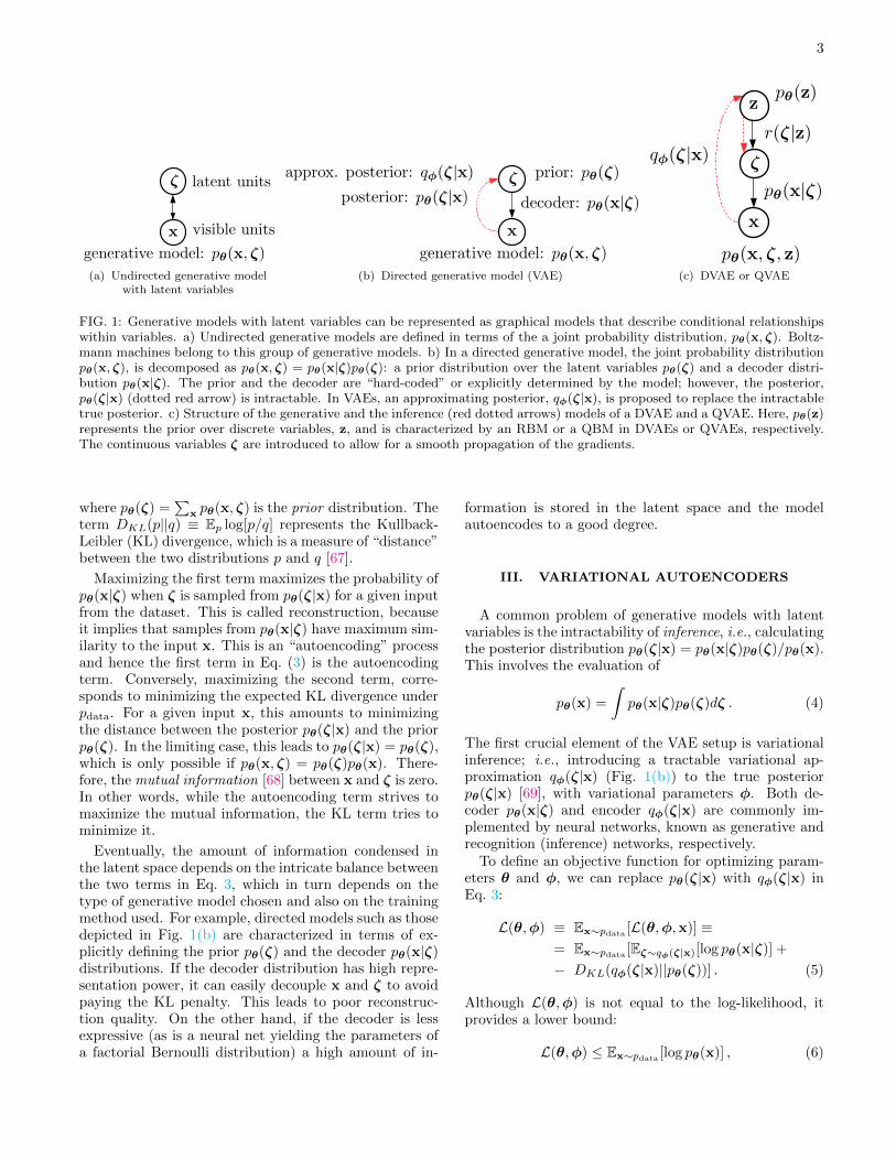
The conditional relationships among the visible units,x, and latent units, ζ, determine the joint probabilitydistribution, pθ(x, ζ), of a generative model and can berepresented in terms of either undirected (Fig. 1(a)) ordirected (Fig. 1(b)) graphs. Unlike fully visible mod-els, generative models with latent variables can poten-tially learn and encode in the latent space useful rep-resentations of the data. This is an appealing propertythat can be exploited to improve other tasks such as su-pervised and semi-supervised learning (i.e., when only afraction of the input data is labeled) [62] with substan-tial practicality in image search [63], speech analysis [64],genomics [65], drug design [66], and so on.

Training a generative model is commonly done viamaximum likelihood (ML) approach, in which optimalmodel parameters θ∗ are obtained by maximizing thelikelihood of the dataset:∑

x

pdata(x) log pθ(x) = Ex∼pdata [log pθ(x)] , (1)

where pθ(x) =∑

ζ pθ(x, ζ) is the marginal probability

distribution of the visible units and Ex∼pdata [. . . ] meansthe expectation value over x sampled from pdata(x).

To better understand the behavior of generative mod-els with latent variables, we now write Ex∼pdata [log pθ(x)]in a more insightful form. First, note that log pθ(x) =Eζ∼pθ(ζ|x)[log pθ(x)], since pθ(x) is independent of ζ.The quantity pθ(ζ|x) is called the posterior distribution,since it represents the probability of the latent variablesafter an observation x has been made (see Fig. 1(b)).Also, since we have pθ(x) = pθ(x, ζ)/pθ(ζ|x), we canwrite:

Ex∼pdata [log pθ(x)] =

= Ex∼pdata

[Eζ∼pθ(ζ|x)

[log

pθ(x, ζ)

pθ(ζ|x)

]]. (2)

By noticing that pθ(ζ,x) = pθ(ζ)pθ(x|ζ) and rearrang-ing Eq. 2, we have:

Ex∼pdata [log pθ(x)] = Ex∼pdata

[Eζ∼pθ(ζ|x)[log pθ(x|ζ)]

−Eζ∼pθ(ζ|x)

[log

pθ(ζ|x)

pθ(ζ)︸ ︷︷ ︸DKL(pθ(ζ|x)||pθ(ζ))

]], (3)

3

(a) Undirected generative modelwith latent variables

(b) Directed generative model (VAE) (c) DVAE or QVAE

FIG. 1: Generative models with latent variables can be represented as graphical models that describe conditional relationshipswithin variables. a) Undirected generative models are defined in terms of the a joint probability distribution, pθ(x, ζ). Boltz-mann machines belong to this group of generative models. b) In a directed generative model, the joint probability distributionpθ(x, ζ), is decomposed as pθ(x, ζ) = pθ(x|ζ)pθ(ζ): a prior distribution over the latent variables pθ(ζ) and a decoder distri-bution pθ(x|ζ). The prior and the decoder are “hard-coded” or explicitly determined by the model; however, the posterior,pθ(ζ|x) (dotted red arrow) is intractable. In VAEs, an approximating posterior, qφ(ζ|x), is proposed to replace the intractabletrue posterior. c) Structure of the generative and the inference (red dotted arrows) models of a DVAE and a QVAE. Here, pθ(z)represents the prior over discrete variables, z, and is characterized by an RBM or a QBM in DVAEs or QVAEs, respectively.The continuous variables ζ are introduced to allow for a smooth propagation of the gradients.

where pθ(ζ) =∑

x pθ(x, ζ) is the prior distribution. Theterm DKL(p||q) ≡ Ep log[p/q] represents the Kullback-Leibler (KL) divergence, which is a measure of “distance”between the two distributions p and q [67].

Maximizing the first term maximizes the probability ofpθ(x|ζ) when ζ is sampled from pθ(ζ|x) for a given inputfrom the dataset. This is called reconstruction, becauseit implies that samples from pθ(x|ζ) have maximum sim-ilarity to the input x. This is an “autoencoding” processand hence the first term in Eq. (3) is the autoencodingterm. Conversely, maximizing the second term, corre-sponds to minimizing the expected KL divergence underpdata. For a given input x, this amounts to minimizingthe distance between the posterior pθ(ζ|x) and the priorpθ(ζ). In the limiting case, this leads to pθ(ζ|x) = pθ(ζ),which is only possible if pθ(x, ζ) = pθ(ζ)pθ(x). There-fore, the mutual information [68] between x and ζ is zero.In other words, while the autoencoding term strives tomaximize the mutual information, the KL term tries tominimize it.

Eventually, the amount of information condensed inthe latent space depends on the intricate balance betweenthe two terms in Eq. 3, which in turn depends on thetype of generative model chosen and also on the trainingmethod used. For example, directed models such as thosedepicted in Fig. 1(b) are characterized in terms of ex-plicitly defining the prior pθ(ζ) and the decoder pθ(x|ζ)distributions. If the decoder distribution has high repre-sentation power, it can easily decouple x and ζ to avoidpaying the KL penalty. This leads to poor reconstruc-tion quality. On the other hand, if the decoder is lessexpressive (as is a neural net yielding the parameters ofa factorial Bernoulli distribution) a high amount of in-

formation is stored in the latent space and the modelautoencodes to a good degree.

III. VARIATIONAL AUTOENCODERS

A common problem of generative models with latentvariables is the intractability of inference, i.e., calculatingthe posterior distribution pθ(ζ|x) = pθ(x|ζ)pθ(ζ)/pθ(x).This involves the evaluation of

pθ(x) =

∫pθ(x|ζ)pθ(ζ)dζ . (4)

The first crucial element of the VAE setup is variationalinference; i.e., introducing a tractable variational ap-proximation qφ(ζ|x) (Fig. 1(b)) to the true posteriorpθ(ζ|x) [69], with variational parameters φ. Both de-coder pθ(x|ζ) and encoder qφ(ζ|x) are commonly im-plemented by neural networks, known as generative andrecognition (inference) networks, respectively.

To define an objective function for optimizing param-eters θ and φ, we can replace pθ(ζ|x) with qφ(ζ|x) inEq. 3:

L(θ,φ) ≡ Ex∼pdata [L(θ,φ,x)] ≡= Ex∼pdata [Eζ∼qφ(ζ|x)[log pθ(x|ζ)] +

− DKL(qφ(ζ|x)||pθ(ζ))] . (5)

Although L(θ,φ) is not equal to the log-likelihood, itprovides a lower bound:

L(θ,φ) ≤ Ex∼pdata [log pθ(x)] , (6)

4

as we show below. Because of this important property,L(θ,φ) is called the evidence (variational) lower bound(ELBO). To prove Eq. 6, we note from Eq. 5 that

L(θ,φ,x) = Eζ∼qφ(ζ|x)

[log pθ(x|ζ)− log

qφ(ζ|x)

pθ(ζ)

]=

= Eζ∼qφ(ζ|x)

[log

pθ(x, ζ)

qφ(ζ|x)

](7)

where we have used pθ(x, ζ) = pθ(ζ)pθ(x|ζ). Eq. 7 is acompact way of expressing the ELBO, which will be usedlater. One may further use pθ(x, ζ) = pθ(x)pθ(ζ|x) toobtain yet another way of writing the ELBO:

L(θ,φ,x) = log pθ(x)− Eζ∼qφ(ζ|x)

[log

qφ(ζ|x)

pθ(ζ|x)

]= log pθ(x)−DKL(qφ(ζ|x)||pθ(ζ|x))]. (8)

Since KL divergence is always non-negative, we obtain

L(θ,φ,x) ≤ log pθ(x), (9)

which immediately gives Eq. 6.It is evident from Eq. 8 that the difference between

the ELBO and the true log-likelihood, i.e., the tightnessof the bound, depends on the distance between the ap-proximate and true posteriors. Maximizing the ELBO,therefore, increases the log-likelihood and decreases thedistance between the two posterior distributions at thesame time. Success in minimizing the bound between thelog-likelihood and ELBO depends on the flexibility andrepresentational power of qφ(ζ|x). However, increasingthe representational power of qφ(ζ|x) does not guaranteesuccess in encoding the information in the latent space.In other words, the widespread problem [70–74] of “ig-noring the latent code” in VAEs is not completely anartifact of choosing a family of approximating posteriordistributions with limited representational power. As wediscussed before, it is rather an intrinsic feature of gen-erative models with latent variables due to the clash ofthe two terms in the objective function defined in Eq. 3.

A. The reparameterization trick

The objective function in Eq. 7 contains expectationvalues of functions of the latent variables ζ under the pos-terior distribution qφ(ζ|x). To train the model, we needto calculate the derivatives of these terms with respectto θ and φ. However, evaluating the derivatives withrespect to φ is problematic because the expectations ofEq. 7 are estimated using samples that are generated ac-cording to a probability distribution that depends on φ.A naive solution to the problem of calculating ∂φ of theexpected value of an arbitrary function Eζ∼qφ [f(ζ)], is touse the identity ∂φqφ = qφ∂φ log qφ, to write

∂φEζ∼qφ [f(ζ)] = Eζ∼qφ [f(ζ)∂φ log qφ] . (10)

Here, for simplicity we assumed that f does not dependon φ. This approach is known as the REINFORCE. How-ever, the expectation of Eq. 10 has high variance and re-quires intricate variance-reduction mechanisms to be ofpractical use [75].

A better approach is to write the random variable ζas a deterministic function of the distribution parame-ters φ and of an additional auxiliary random variable ρ.The latter is given by a probability distribution p(ρ) thatdoes not depend on φ. This reparameterization, ζ(φ,ρ),can be used to write Eζ∼qφ [f(ζ)] = Eρ∼p(ρ)[f(ζ(φ,ρ))].Therefore, we can move the derivative inside the expec-tation with no difficulty:

∂φEζ∼qφ [f(ζ)] = Eρ∼p(ρ) [∂φf(ζ(φ,ρ))] . (11)

This is called the reparameterization trick [53] and ismostly responsible for the recent success and prolifera-tion of VAEs. When applied to Eq. 7, we have:

L(θ,φ,x) = Eζ∼qφ(ζ|x)

[log

pθ(x, ζ)

qφ(ζ|x)

]= Eρ∼p(ρ)

[log

pθ(x, ζ(φ,ρ))

qφ(ζ(φ,ρ)|x)

], (12)

where we have suppressed the inclusion of x in the ar-guments of the reparameterized ζ to keep the notationuncluttered.

It is now important to find a function ζ(φ,ρ) such thatρ becomes φ-independent. Let us define a function F

ρ ≡ Fφ(ζ). (13)

The probability distributions p(ρ) and qφ(ζ|x) shouldsatisfy p(ρ)dρ = qφ(ζ|x)dζ, therefore

p(ρ) =qφ(ζ|x)

dρ/dζ=

qφ(ζ|x)

dFφ(ζ)/dζ. (14)

To have p(ρ) independent of φ we need

Fφ(ζ) =

∫ ζ

0

qφ(ζ′|x)dζ′. (15)

Now, by choosing Fφ to be the cumulative distributionfunction (CDF) of qφ(ζ|x), p(ρ) becomes a uniform dis-tribution U(0, 1) for ρ ∈ [0, 1]. We can thus write

ζ(φ,ρ) = F−1φ (ρ) . (16)

To derive Eq. 16, we have implicitly assumed that thelatent variables are continuous and that the posteriorfactorizes: qφ(ζ|x) =

∏l qφ(ζl|x). It is possible to ex-

tend the reparameterization trick to include discrete la-tent variables (see next section) and more complicatedapproximate posteriors (see Appendix C).

5

IV. VAE WITH DISCRETE LATENT SPACE

Most of the VAEs studied so far have continuous latentspaces due to the difficulty of propagating derivativesthrough discrete variables. Nonetheless, discrete stochas-tic units are indispensable to representing distributions insupervised and unsupervised learning, attention models,language modeling and reinforcement learning [76]. Somenoteworthy examples include application of discrete unitsin learning distinct semantic classes [62] and in semisu-pervised generation [77] to learn more meaningful hier-archical VAEs. In Ref. [78], when the latent space iscomposed of discrete variables, the representations learnto disentangle content and style information of images inan unsupervised fashion.

Due to the non-differentiability of discrete stochasticunits, several methods that involve variational inferenceuse the REINFORCE method, Eq. 10, from the rein-forcement learning literature [75, 79, 80]. However, thesemethods yield noisy estimates of gradients that need tobe mitigated using several variance reduction techniquessuch as finding appropriate control variates. Another ap-proach involves using biased derivatives for the Bernoullivariables [81]. There are also two approaches that ex-tend the reparameterization trick to discrete variables.Refs. [76, 82] concurrently came up with a relaxationof categorical discrete units into continuous variables byadding Gumbel noise to the logits inside a softmax func-tion, with a temperature hyper-parameter. The soft-max function transforms into a non-differentiable argmaxfunction obtaining unbiased samples in the limit of zerotemperature. However, in this limit the training stopssince variables become truly discrete. Therefore, an an-nealing schedule is used for the temperature throughoutthe training to obtain less noisy, yet biased, estimates ofgradients [76].

Here we follow the approach proposed in [55], whichyields reparameterizable and unbiased estimates of gradi-ents. As discussed in the previous section, the generativeprocess in a VAE involves sampling a set of continuousvariables ζ ∼ pθ(ζ). To implement a DVAE, we assumethe prior distribution is now defined on a set of discretevariables z ∼ pθ(z), with z ∈ {0, 1}L. Once again we useθ to denote collective parameters of the generative sideof the model. To propagate the gradients through thediscrete variables, we keep the variables ζ as an auxiliaryset of continuous variables [55]. The full prior is chosenas follows (Fig. 1(c)) :

pθ(ζ, z) ≡ r(ζ|z)pθ(z) ≡

(L∏l=1

r(ζl|zl)

)pθ(z) . (17)

The newly introduced term r(ζ|z) acts as a smoothingprobability distribution that enables the implementationof the reparameterization trick. The structure of theDVAE is completed by considering a particular form forthe approximating posterior and marginal distributions

(Fig. 1(c)):

qφ(ζ, z|x) ≡ r(ζ|z)qφ(z|x)

pθ(x|ζ, z) ≡ pθ(x|ζ) , (18)

where for now we assume qφ(z|x) =∏l qφ(zl|x) is a prod-

uct of Bernoulli probabilities for the discrete variable zl(see again Appendix C for the case where hierarchies arepresent in the posterior). With the above choice, theELBO bound can be written as

L(θ,φ,x) = Eqφ(ζ|x)[log pθ(x|ζ)] +

− DKL(qφ(z|x)||pθ(z)) , (19)

where qφ(ζ|x) is the approximate posterior marginalizedover the discrete variables. In the equation above wehave used the fact that the KL term does not explic-itly depend on ζ while the autoencoding term does notexplicitly depend on z.

A. The reparameterization trick for DVAE

We can apply the inverse CDF reparameterizationtrick, Eq. 16, to the autoencoding term in Eq. 19 if wechoose the function r(ζ|z) such that the CDF of the ap-proximating posterior marginalized over the discrete vari-ables

F(ζ) ≡∫ ζ

0

qφ(ζ′|x)dζ′ (20)

can be inverted:

Eqφ(ζ|x)[log pθ(x|ζ)] = Eρ∼U [log pθ(x|F−1(ρ)] . (21)

An appropriate choice for r(ζl|zl) is, for example, thespike-and-exponential transformation:

r(ζl|zl = 0) = δ(ζl)

r(ζl|zl = 1) =

{β eβζl

eβ−1, if 0 < ζl ≤ 1

0, otherwise .(22)

For this distribution we can write:

Fl(ζl) =

∫ ζl

0

qφ(ζ ′l |x)dζ ′l =

∫ ζl

0

∑zl=0,1

qφ(zl|x)r(ζ ′l |zl)dζ ′l .

(23)Using Eq. 22 with Bernoulli distribution qφ(zl=1|x) = qland qφ(zl=0|x) = 1−ql, we find

ρl = qleβζl − 1

eβ − 1+ (1− ql) , (24)

which can be easily inverted to obtain ζl

ζl(ρl, ql) =1

βlog

[(max(ρl+ql−1, 0)

ql

)(eβ−1) + 1

].

(25)

6

The virtue of the spike-and-exponential smoothing distri-bution is that zl can be deterministically obtained fromζl and thus ρl:

zl(ρl, ql) = sign(ζl(ρl, ql)) = Θ(ρl+ql−1) , (26)

which follows from Eqs 22 and 25. This property is cru-cial to apply the reparameterization trick to the KL term,as shown below, and evaluating its derivatives as shownin Appendix D.

For later convenience, we note that the KL term canbe written as the difference between an entropy term,H(qφ(z|x)), and a cross-entropy term, H(qφ(z|x), pθ(z)):

DKL(qφ(z|x)||pθ(z)) = Eqφ [log qφ]︸ ︷︷ ︸−H(qφ)

−Eqφ [log pθ]︸ ︷︷ ︸−H(qφ,pθ)

.

Herein, for simplicity, we use qφ and pθ in place of qφ(z|x)and pθ(z), respectively, in unambiguous cases. UsingEq. 26, the reparameterization trick can be applied tothe entropy term:

H(qφ) ≡ −Ez∼qφ [log qφ] = −Eρ∼U [log qφ(z(ρ,φ)|x)],

(27)

where we have explicitly shown the dependence ofz on ρ and φ. Note that in the simple case ofa factorial Bernoulli distribution, we do not needto use the reparameterization trick and can usethe analytic form of the entropy; i.e., H(qφ) =

−∑Ll=1 (ql log ql + (1− ql) log(1− ql)) (see Appendix B

for more details). Similarly, applying the reparameteri-zation trick to the cross-entropy leads to:

−H(qφ, pθ) ≡ Ez∼qφ [log pθ] = Eρ∼U [log pθ(z(ρ,φ))] .(28)

It is a common practice to use hierarchical distribu-tions to achieve more powerful approximating posteriors.Briefly, the latent variables are compartmentalized intoseveral groups, and the probability density function ofeach group depends on the values of the latent variablesin the preceding groups; i.e., qφ(zl|ζm<l,x). This createsa more powerful approximating posterior able to repre-sent more complex correlations between latent variables,as compared to a simple factorial distribution. See Ap-pendix C for more details.

B. DVAE with Boltzmann machines

Boltzmann machines are probabilistic models ableto represent complex multi-modal probability distribu-tions [83], and are thus attractive candidates for the la-tent space of a VAE. This approach is also appealing withregards to the machine-learning application of quantumcomputers. The probability distribution realized by an

RBM is

pθ(z) ≡ e−Eθ(z)/Zθ , Zθ ≡∑z

e−Eθ(z) ,

Eθ(z) =∑l

zlhl +∑l<m

Wlmzlzm, h,W ∈ {θ}. (29)

The negative cross entropy term −H(qφ, pθ) =Ez∼qφ [log pθ] is the log-likelihood of z sampled from theapproximating posterior z ∼ qφ(z|x) under the model pθ.After reparameterization, we have

H(qφ, pθ) = −Eρ∼U [log pθ(z(ρ,φ))]

= Eρ∼U [Eθ(z(ρ,φ))] + logZθ. (30)

Gradients can thus be computed as usual as the differencebetween a positive and negative phase, in which the latteris computed via Boltzmann sampling from the BM:

∂H(qφ, pθ) = Eρ∼U [∂Eθ(z(ρ,φ))]− Ez∼pθ [∂Eθ(z)] .(31)

Notice that the positive phase (the first term above)involves the expectation over the approximating poste-rior, but it is explicitly written in terms of the discretevariables z(ρ,φ). We thus need to calculate the deriva-tives through these variables. We discuss the computa-tion of the positive phase in the most general case inAppendix D.

C. Experimental results with DVAE

In this section, we show that the DVAE model intro-duced in Sec. IV achieves state-of-the-art performance,for variational inference models with only latent vari-ables, on the MNIST dataset [48]. We perform experi-ments with restricted Boltzmann machines, in which thehidden and visible units are placed at the two sides ofa bipartite graph. Notice that in a DVAE setup, all theunits of the (classical) RBM are latent variables (thereis technically no distinction between visible and hiddenunits as for standalone RBMs). We still use an RBMto exploit its bipartite structure enabling efficient Gibbsblock-sampling. This allows us to train DVAEs withRBMs with up to 256 units per layer.

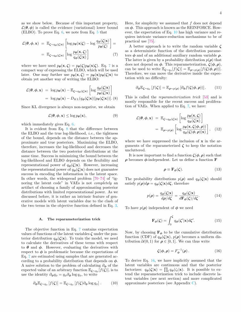
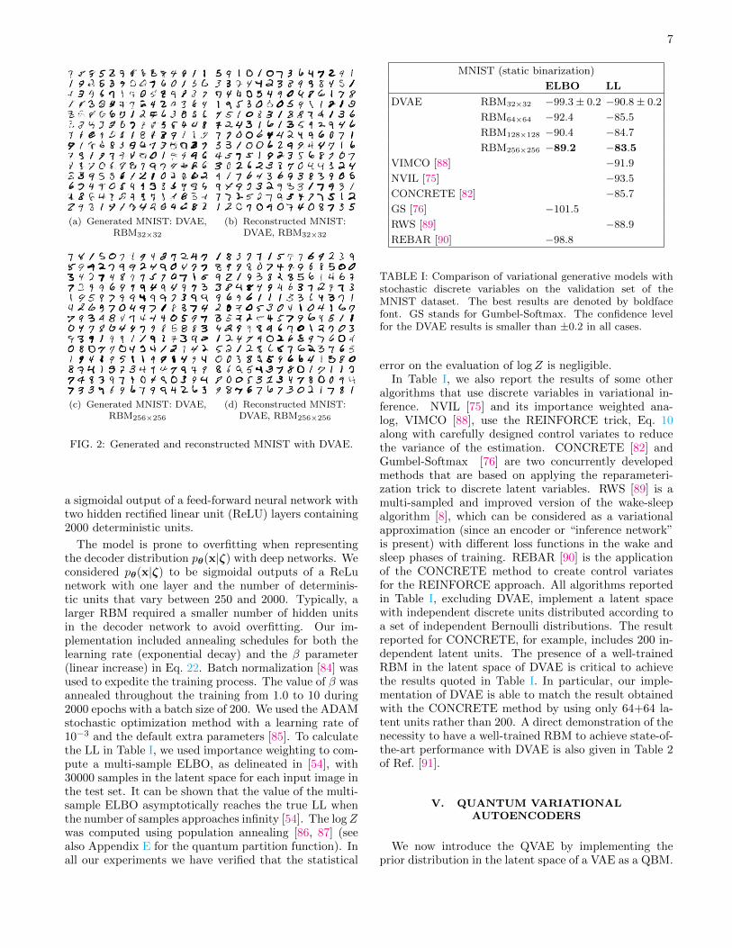
Figure 2 shows generated and reconstructed MNISTdigits for a DVAE with RBMs with 32 and 256 unitsper layer. In Table I, we report the best results for theELBO and log-likelihood (LL) we obtained with RBMs of32, 64, 128, and 256 units per layer. For 256 units, we ob-tained an LL of −83.5±0.2, with the reported error beinga conservative estimate of our statistical uncertainty. Inall cases, the negative phase of the RBMs was estimatedusing persistent contrastive divergence (PCD), with 1000chains and 200 block-Gibbs updates per gradient evalua-tion. We have chosen an approximating posterior with 8levels of hierarchies (the number of units that each levelof hierarchy represents is the total number of latent unitsdivided by 8); each Bernoulli probability qφ(zl|ζm<l,x) is

7

(a) Generated MNIST: DVAE,RBM32×32

(b) Reconstructed MNIST:DVAE, RBM32×32

(c) Generated MNIST: DVAE,RBM256×256

(d) Reconstructed MNIST:DVAE, RBM256×256

FIG. 2: Generated and reconstructed MNIST with DVAE.

a sigmoidal output of a feed-forward neural network withtwo hidden rectified linear unit (ReLU) layers containing2000 deterministic units.

The model is prone to overfitting when representingthe decoder distribution pθ(x|ζ) with deep networks. Weconsidered pθ(x|ζ) to be sigmoidal outputs of a ReLunetwork with one layer and the number of determinis-tic units that vary between 250 and 2000. Typically, alarger RBM required a smaller number of hidden unitsin the decoder network to avoid overfitting. Our im-plementation included annealing schedules for both thelearning rate (exponential decay) and the β parameter(linear increase) in Eq. 22. Batch normalization [84] wasused to expedite the training process. The value of β wasannealed throughout the training from 1.0 to 10 during2000 epochs with a batch size of 200. We used the ADAMstochastic optimization method with a learning rate of10−3 and the default extra parameters [85]. To calculatethe LL in Table I, we used importance weighting to com-pute a multi-sample ELBO, as delineated in [54], with30000 samples in the latent space for each input image inthe test set. It can be shown that the value of the multi-sample ELBO asymptotically reaches the true LL whenthe number of samples approaches infinity [54]. The logZwas computed using population annealing [86, 87] (seealso Appendix E for the quantum partition function). Inall our experiments we have verified that the statistical

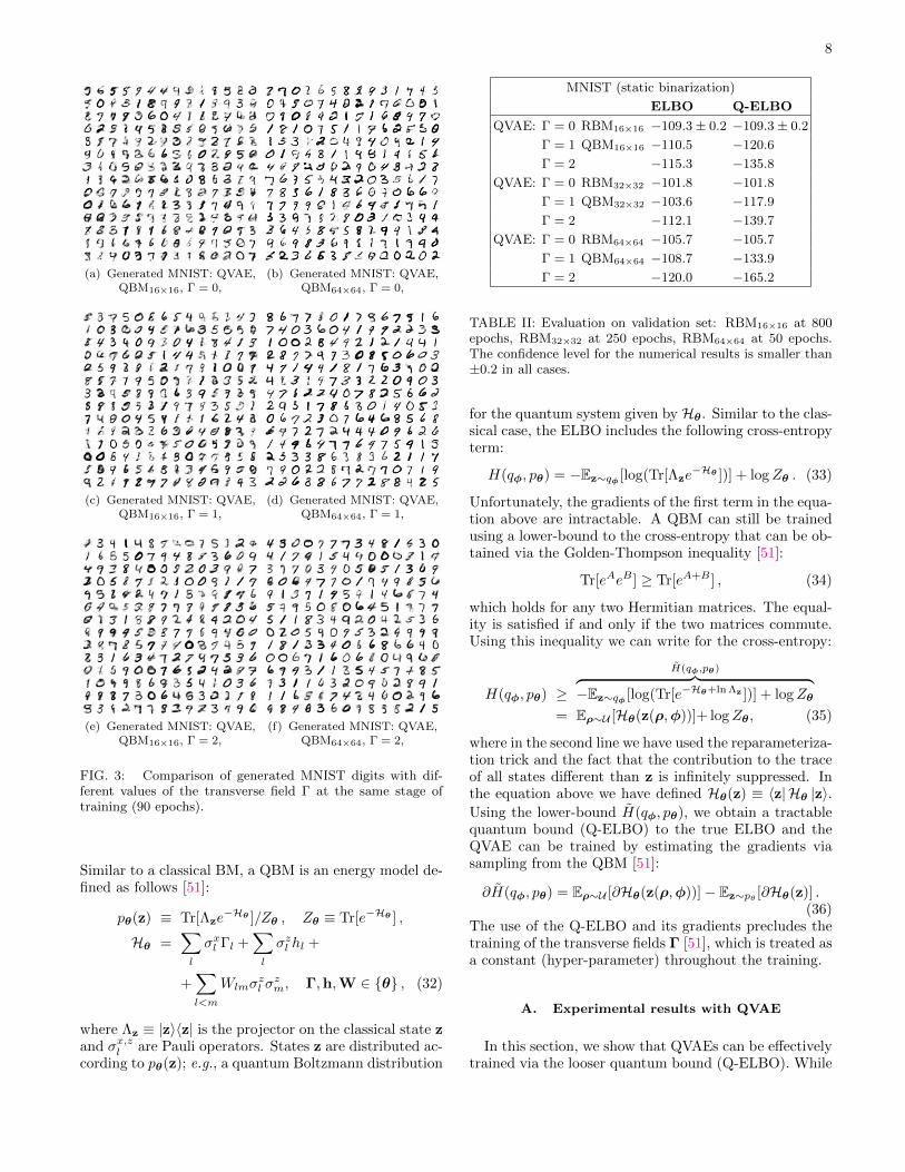
MNIST (static binarization)

ELBO LL

DVAE RBM32×32 −99.3± 0.2 −90.8± 0.2

RBM64×64 −92.4 −85.5

RBM128×128 −90.4 −84.7

RBM256×256 −89.2 −83.5VIMCO [88] −91.9

NVIL [75] −93.5

CONCRETE [82] −85.7

GS [76] −101.5

RWS [89] −88.9

REBAR [90] −98.8

TABLE I: Comparison of variational generative models withstochastic discrete variables on the validation set of theMNIST dataset. The best results are denoted by boldfacefont. GS stands for Gumbel-Softmax. The confidence levelfor the DVAE results is smaller than ±0.2 in all cases.

error on the evaluation of logZ is negligible.In Table I, we also report the results of some other

algorithms that use discrete variables in variational in-ference. NVIL [75] and its importance weighted ana-log, VIMCO [88], use the REINFORCE trick, Eq. 10along with carefully designed control variates to reducethe variance of the estimation. CONCRETE [82] andGumbel-Softmax [76] are two concurrently developedmethods that are based on applying the reparameteri-zation trick to discrete latent variables. RWS [89] is amulti-sampled and improved version of the wake-sleepalgorithm [8], which can be considered as a variationalapproximation (since an encoder or “inference network”is present) with different loss functions in the wake andsleep phases of training. REBAR [90] is the applicationof the CONCRETE method to create control variatesfor the REINFORCE approach. All algorithms reportedin Table I, excluding DVAE, implement a latent spacewith independent discrete units distributed according toa set of independent Bernoulli distributions. The resultreported for CONCRETE, for example, includes 200 in-dependent latent units. The presence of a well-trainedRBM in the latent space of DVAE is critical to achievethe results quoted in Table I. In particular, our imple-mentation of DVAE is able to match the result obtainedwith the CONCRETE method by using only 64+64 la-tent units rather than 200. A direct demonstration of thenecessity to have a well-trained RBM to achieve state-of-the-art performance with DVAE is also given in Table 2of Ref. [91].

V. QUANTUM VARIATIONALAUTOENCODERS

We now introduce the QVAE by implementing theprior distribution in the latent space of a VAE as a QBM.

8

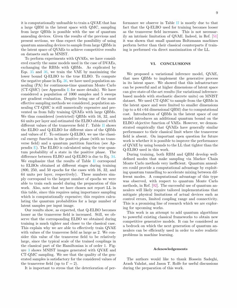
(a) Generated MNIST: QVAE,QBM16×16, Γ = 0,

(b) Generated MNIST: QVAE,QBM64×64, Γ = 0,

(c) Generated MNIST: QVAE,QBM16×16, Γ = 1,

(d) Generated MNIST: QVAE,QBM64×64, Γ = 1,

(e) Generated MNIST: QVAE,QBM16×16, Γ = 2,

(f) Generated MNIST: QVAE,QBM64×64, Γ = 2,

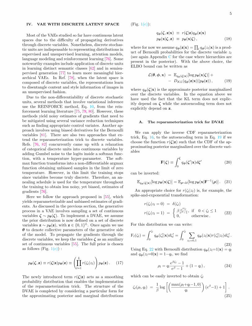
FIG. 3: Comparison of generated MNIST digits with dif-ferent values of the transverse field Γ at the same stage oftraining (90 epochs).

Similar to a classical BM, a QBM is an energy model de-fined as follows [51]:

pθ(z) ≡ Tr[Λze−Hθ ]/Zθ , Zθ ≡ Tr[e−Hθ ] ,

Hθ =∑l

σxl Γl +∑l

σzl hl +

+∑l<m

Wlmσzl σ

zm, Γ,h,W ∈ {θ} , (32)

where Λz ≡ |z〉〈z| is the projector on the classical state zand σx,zl are Pauli operators. States z are distributed ac-cording to pθ(z); e.g., a quantum Boltzmann distribution

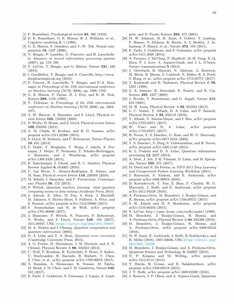
MNIST (static binarization)

ELBO Q-ELBO

QVAE: Γ = 0 RBM16×16 −109.3± 0.2 −109.3± 0.2

Γ = 1 QBM16×16 −110.5 −120.6

Γ = 2 −115.3 −135.8

QVAE: Γ = 0 RBM32×32 −101.8 −101.8

Γ = 1 QBM32×32 −103.6 −117.9

Γ = 2 −112.1 −139.7

QVAE: Γ = 0 RBM64×64 −105.7 −105.7

Γ = 1 QBM64×64 −108.7 −133.9

Γ = 2 −120.0 −165.2

TABLE II: Evaluation on validation set: RBM16×16 at 800epochs, RBM32×32 at 250 epochs, RBM64×64 at 50 epochs.The confidence level for the numerical results is smaller than±0.2 in all cases.

for the quantum system given by Hθ. Similar to the clas-sical case, the ELBO includes the following cross-entropyterm:

H(qφ, pθ) = −Ez∼qφ [log(Tr[Λze−Hθ ])] + logZθ . (33)

Unfortunately, the gradients of the first term in the equa-tion above are intractable. A QBM can still be trainedusing a lower-bound to the cross-entropy that can be ob-tained via the Golden-Thompson inequality [51]:

Tr[eAeB ] ≥ Tr[eA+B ] , (34)

which holds for any two Hermitian matrices. The equal-ity is satisfied if and only if the two matrices commute.Using this inequality we can write for the cross-entropy:

H(qφ, pθ) ≥

H(qφ,pθ)︷ ︸︸ ︷−Ez∼qφ [log(Tr[e−Hθ+ln Λz ])] + logZθ

= Eρ∼U [Hθ(z(ρ,φ))]+ logZθ, (35)

where in the second line we have used the reparameteriza-tion trick and the fact that the contribution to the traceof all states different than z is infinitely suppressed. Inthe equation above we have defined Hθ(z) ≡ 〈z|Hθ |z〉.Using the lower-bound H(qφ, pθ), we obtain a tractablequantum bound (Q-ELBO) to the true ELBO and theQVAE can be trained by estimating the gradients viasampling from the QBM [51]:

∂H(qφ, pθ) = Eρ∼U [∂Hθ(z(ρ,φ))]− Ez∼pθ [∂Hθ(z)] .(36)

The use of the Q-ELBO and its gradients precludes thetraining of the transverse fields Γ [51], which is treated asa constant (hyper-parameter) throughout the training.

A. Experimental results with QVAE

In this section, we show that QVAEs can be effectivelytrained via the looser quantum bound (Q-ELBO). While

9

it is computationally unfeasible to train a QVAE that hasa large QBM in the latent space with QMC, samplingfrom large QBMs is possible with the use of quantumannealing devices. Given the results of the previous andpresent sections, we thus expect the possibility of usingquantum annealing devices to sample from large QBMs inthe latent space of QVAEs to achieve competitive resultson datasets such as MNIST.

To perform experiments with QVAEs, we have consid-ered exactly the same models used in the case of DVAEs,exchanging the RBMs with QBMs. As explicated byEqs. 35 and 36, we train the VAE by maximizing thelower bound Q-ELBO to the true ELBO. To computethe negative phase in Eq. 36, we have used population an-nealing (PA) for continuous-time quantum Monte Carlo(CT-QMC) (see Appendix E for more details). We haveconsidered a population of 1000 samples and 5 sweepsper gradient evaluation. Despite being one of the mosteffective sampling methods we considered, population an-nealing CT-QMC is still numerically expensive and pre-vented us from fully training QVAEs with large QBMs.We thus considered (restricted) QBMs with 16, 32, and64 units per layer and estimated the ELBO obtained withdifferent values of the transverse field Γ. Table II showsthe ELBO and Q-ELBO for different sizes of the QBMsand values of Γ. To estimate Q-ELBO, we use the classi-cal energy function in the positive phase (with no trans-verse field) and a quantum partition function (see Ap-pendix E). The ELBO is calculated using the true quan-tum probability of a state in the positive phase. Thedifference between ELBO and Q-ELBO is due to Eq. 34.We emphasize that the results of Table II correspondto ELBOs obtained at different stages during training(800, 250, and 50 epochs for the cases with 16, 32, and64 units per layer, respectively). These numbers sim-ply correspond to the largest number of epochs we wereable to train each model during the preparation of thiswork. Also, note that we have chosen not report LL inthis table, since this requires using importance samplingwhich is computationally expensive; this requires calcu-lating the quantum probabilities for a large number oflatent samples per input image.

Our results show, as expected, that Q-ELBO becomeslooser as the transverse field is increased. Still, we ob-serve that the corresponding ELBO we obtained duringtraining is much tighter and closer to the classical case.This explain why we are able to effectively train QVAEwith values of the transverse field as large as 2. We con-sider this value of the transverse field to be relativelylarge, since the typical scale of the trained couplings inthe classical part of the Hamiltonian is of order 1. Fig-ure 3 shows MNIST images generated with QVAE andCT-QMC sampling. We see that the quality of the gen-erated samples is satisfactory for the considered values ofthe transverse field (up to Γ = 2).

It is important to stress that the deterioration of per-

formance we observe in Table II is mostly due to thatfact that the Q-ELBO used for training becomes looseras the transverse field increases. This is not necessar-ily an intrinsic limitation of QVAE. Indeed, in Ref. [51]it was shown that small quantum Boltzmann machinesperform better than their classical counterparts if train-ing is performed via direct maximization of the LL.

VI. CONCLUSIONS

We proposed a variational inference model, QVAE,that uses QBMs to implement the generative processin its latent space. We showed that this infrastructurecan be powerful and at higher dimensions of latent spacecan give state-of-the-art results (for variational inference-based models with stochastic discrete units) on MNISTdataset. We used CT-QMC to sample from the QBMs inthe latent space and were limited to smaller dimensions(up to a 64×64 dimensional QBM) due to computationalcost. Introduction of QBMs in the latent space of ourmodel introduces an additional quantum bound on theELBO objective function of VAEs. However, we demon-strated empirically that QVAEs have generally similarperformance to their classical limit where the transversefield is absent. On important open question for futurework is whether it is possible to improve the performanceof QVAE by using bounds to the LL that tighter than theQ-ELBO used in this work.

During training, both RBM and QBM develop well-defined modes that make sampling via Markov ChainMonte Carlo methods very inefficient. Quantum anneal-ers could provide a computational advantage by exploit-ing quantum tunnelling to accelerate mixing between dif-ferent modes. A computational advantage of this typewas observed, with respect to quantum Monte Carlomethods, in Ref. [92]. The successful use of quantum an-nealers will likely require tailored implementations thatmitigate physical limitations of actual devices such ascontrol errors, limited coupling range and connectivity.This is a promising line of research which we are explor-ing for upcoming works.

This work is an attempt to add quantum algorithmsto powerful existing classical frameworks to obtain newcompetitive generative models. It can be considered asa bedrock on which the next generation of quantum an-nealers can be efficiently used in order to solve realisticproblems in machine learning.

Acknowledgements

The authors would like to thank Hossein Sadeghi,Arash Vahdat, and Jason T. Rolfe for useful discussionsduring the preparation of this work.

10

[1] F. Rosenblatt, Psychological review 65, 386 (1958).[2] D. E. Rumelhart, G. E. Hinton, R. J. Williams, et al.,

Cognitive modeling 5, 1 (1988).[3] G. E. Hinton, S. Osindero, and Y.-W. Teh, Neural com-

putation 18, 1527 (2006).[4] Y. Bengio, P. Lamblin, D. Popovici, and H. Larochelle,

in Advances in neural information processing systems(2007), pp. 153–160.

[5] Y. LeCun, Y. Bengio, and G. Hinton, Nature 521, 436(2015).

[6] I. Goodfellow, Y. Bengio, and A. Courville, http://www.deeplearningbook.org (2016).

[7] P. Vincent, H. Larochelle, Y. Bengio, and P.-A. Man-zagol, in Proceedings of the 25th international conferenceon Machine learning (ACM, 2008), pp. 1096–1103.

[8] G. E. Hinton, P. Dayan, B. J. Frey, and R. M. Neal,Science 268, 1158 (1995).

[9] T. Tieleman, in Proceedings of the 25th internationalconference on Machine learning (ACM, 2008), pp. 1064–1071.

[10] A. W. Harrow, A. Hassidim, and S. Lloyd, Physical re-view letters 103, 150502 (2009).

[11] N. Wiebe, D. Braun, and S. Lloyd, Physical review letters109, 050505 (2012).

[12] A. M. Childs, R. Kothari, and R. D. Somma, arXivpreprint arXiv:1511.02306 (2015).

[13] S. Lloyd, M. Mohseni, and P. Rebentrost, Nature Physics10, 631 (2014).

[14] F. Dolde, V. Bergholm, Y. Wang, I. Jakobi, S. Pez-zagna, J. Meijer, P. Neumann, T. Schulte-Herbruggen,J. Biamonte, and J. Wrachtrup, arXiv preprintarXiv:1309.4430 (2013).

[15] E. Zahedinejad, J. Ghosh, and B. C. Sanders, PhysicalReview Applied 6, 054005 (2016).

[16] U. Las Heras, U. Alvarez-Rodriguez, E. Solano, andM. Sanz, Physical review letters 116, 230504 (2016).

[17] M. Schuld, I. Sinayskiy, and F. Petruccione, Contempo-rary Physics 56, 172 (2015).

[18] P. Wittek, Quantum machine learning: what quantumcomputing means to data mining (Academic Press, 2014).

[19] J. Adcock, E. Allen, M. Day, S. Frick, J. Hinchliff,M. Johnson, S. Morley-Short, S. Pallister, A. Price, andS. Stanisic, arXiv preprint arXiv:1512.02900 (2015).

[20] S. Arunachalam and R. de Wolf, arXiv preprintarXiv:1701.06806 (2017).

[21] J. Biamonte, P. Wittek, N. Pancotti, P. Rebentrost,N. Wiebe, and S. Lloyd, Nature 549, 195 (2017),1611.09347, URL https://arxiv.org/abs/1611.09347.

[22] M. A. Nielsen and I. Chuang, Quantum computation andquantum information (2002).

[23] D. A. Lidar and T. A. Brun, Quantum error correction(Cambridge University Press, 2013).

[24] A. G. Fowler, M. Mariantoni, J. M. Martinis, and A. N.Cleland, Physical Review A 86, 032324 (2012).

[25] C. Neill, P. Roushan, K. Kechedzhi, S. Boixo, S. Isakov,V. Smelyanskiy, R. Barends, B. Burkett, Y. Chen,Z. Chen, et al., arXiv preprint arXiv:1709.06678 (2017).

[26] A. Kandala, A. Mezzacapo, K. Temme, M. Takita,M. Brink, J. M. Chow, and J. M. Gambetta, Nature 549,242 (2017).

[27] E. Farhi, J. Goldstone, S. Gutmann, J. Lapan, A. Lund-

gren, and D. Preda, Science 292, 472 (2001).[28] M. W. Johnson, M. H. Amin, S. Gildert, T. Lanting,

F. Hamze, N. Dickson, R. Harris, A. J. Berkley, J. Jo-hansson, P. Bunyk, et al., Nature 473, 194 (2011).

[29] E. Farhi, J. Goldstone, and S. Gutmann, arXiv preprintarXiv:1411.4028 (2014).

[30] A. Peruzzo, J. McClean, P. Shadbolt, M.-H. Yung, X.-Q.Zhou, P. J. Love, A. Aspuru-Guzik, and J. L. O’brien,Nature communications 5 (2014).

[31] J. Otterbach, R. Manenti, N. Alidoust, A. Bestwick,M. Block, B. Bloom, S. Caldwell, N. Didier, E. S. Fried,S. Hong, et al., arXiv preprint arXiv:1712.05771 (2017).

[32] T. Kadowaki and H. Nishimori, Physical Review E 58,5355 (1998).

[33] G. E. Santoro, R. Martonak, E. Tosatti, and R. Car,Science 295, 2427 (2002).

[34] J. Brooke, T. Rosenbaum, and G. Aeppli, Nature 413,610 (2001).

[35] M. H. Amin, Physical Review A 92, 052323 (2015).[36] L. C. Venuti, T. Albash, D. A. Lidar, and P. Zanardi,

Physical Review A 93, 032118 (2016).[37] T. Albash, V. Martin-Mayor, and I. Hen, arXiv preprint

arXiv:1703.03871 (2017).[38] W. Vinci and D. A. Lidar, arXiv preprint

arXiv:1710.07871 (2017).[39] H. Neven, V. S. Denchev, G. Rose, and W. G. Macready,

arXiv preprint arXiv:0811.0416 (2008).[40] V. S. Denchev, N. Ding, S. Vishwanathan, and H. Neven,

arXiv preprint arXiv:1205.1148 (2012).[41] K. L. Pudenz and D. A. Lidar, Quantum information

processing 12, 2027 (2013).[42] A. Mott, J. Job, J.-R. Vlimant, D. Lidar, and M. Spirop-

ulu, Nature 550, 375 (2017).[43] M. Denil and N. De Freitas, in NIPS 2011 Deep Learning

and Unsupervised Feature Learning Workshop (2011).[44] J. Raymond, S. Yarkoni, and E. Andriyash, arXiv

preprint arXiv:1606.00919 (2016).[45] D. Korenkevych, Y. Xue, Z. Bian, F. Chudak, W. G.

Macready, J. Rolfe, and E. Andriyash, arXiv preprintarXiv:1611.04528 (2016).

[46] A. Perdomo-Ortiz, M. Benedetti, J. Realpe-Gomez, andR. Biswas, arXiv preprint arXiv:1708.09757 (2017).

[47] S. H. Adachi and M. P. Henderson, arXiv preprintarXiv:1510.06356 (2015).

[48] Y. LeCun, http://yann. lecun. com/exdb/mnist/ (1998).[49] M. Benedetti, J. Realpe-Gomez, R. Biswas, and

A. Perdomo-Ortiz, Physical Review A 94, 022308 (2016).[50] M. Benedetti, J. Realpe-Gomez, R. Biswas, and

A. Perdomo-Ortiz, arXiv preprint arXiv:1609.02542(2016).

[51] M. H. Amin, E. Andriyash, J. Rolfe, B. Kulchytskyy, andR. Melko (2016), 1601.02036, URL https://arxiv.org/

abs/1601.02036.[52] M. Benedetti, J. Realpe-Gomez, and A. Perdomo-Ortiz,

Quantum Science and Technology 3, 034007 (2018).[53] D. P. Kingma and M. Welling, arXiv preprint

arXiv:1312.6114 (2013).[54] Y. Burda, R. Grosse, and R. Salakhutdinov, arXiv

preprint arXiv:1509.00519 (2015).[55] J. T. Rolfe, arXiv preprint arXiv:1609.02200 (2016).[56] J. Romero, J. P. Olson, and A. Aspuru-Guzik, Quantum

11

Science and Technology 2, 045001 (2017).[57] K. H. Wan, O. Dahlsten, H. Kristjansson, R. Gardner,

and M. Kim, npj Quantum Information 3, 36 (2017).[58] I. J. Goodfellow, J. Pouget-Abadie, M. Mirza, B. Xu,

D. Warde-Farley, S. Ozair, A. Courville, and Y. Bengio,arXiv:1406.2661 [cs, stat] (2014), arXiv: 1406.2661, URLhttp://arxiv.org/abs/1406.2661.

[59] B. Uria, M.-A. Cote, K. Gregor, I. Murray, andH. Larochelle, Journal of Machine Learning Research 17,1 (2016).

[60] M. Germain, K. Gregor, I. Murray, and H. Larochelle,in Proceedings of the 32nd International Conference onMachine Learning (ICML-15) (2015), pp. 881–889.

[61] A. v. d. Oord, N. Kalchbrenner, and K. Kavukcuoglu,arXiv preprint arXiv:1601.06759 (2016).

[62] D. P. Kingma, S. Mohamed, D. J. Rezende, andM. Welling, in Advances in Neural Information Process-ing Systems (2014), pp. 3581–3589.

[63] R. Fergus, Y. Weiss, and A. Torralba, in Advances inneural information processing systems (2009), pp. 522–530.

[64] Y. Liu and K. Kirchhoff, in INTERSPEECH (2013), pp.1840–1843.

[65] M. Shi and B. Zhang, Bioinformatics 27, 3017 (2011).[66] H. Chen and Z. Zhang, PloS one 8, e62975 (2013).[67] C. M. Bishop, Pattern Recognition and Machine Learning

(Springer, New York, 2011), 1st ed., ISBN 978-0-387-31073-2.

[68] T. M. Cover and J. A. Thomas, Elements of informationtheory, Wiley series in telecommunications (Wiley, NewYork, 1991), ISBN 978-0-471-06259-2.

[69] M. D. Hoffman, D. M. Blei, C. Wang, and J. Paisley, TheJournal of Machine Learning Research 14, 1303 (2013).

[70] X. Chen, D. P. Kingma, T. Salimans, Y. Duan, P. Dhari-wal, J. Schulman, I. Sutskever, and P. Abbeel, arXivpreprint arXiv:1611.02731 (2016).

[71] S. Zhao, J. Song, and S. Ermon, arXiv preprintarXiv:1706.02262 (2017).

[72] S. Yeung, A. Kannan, Y. Dauphin, and L. Fei-Fei, arXivpreprint arXiv:1706.03643 (2017).

[73] J. M. Tomczak and M. Welling, arXiv preprintarXiv:1705.07120 (2017).

[74] S. Zhao, J. Song, and S. Ermon, arXiv preprintarXiv:1702.08658 (2017).

[75] A. Mnih and K. Gregor, arXiv preprint arXiv:1402.0030(2014).

[76] E. Jang, S. Gu, and B. Poole, arXiv preprintarXiv:1611.01144 (2016).

[77] L. Maaløe, M. Fraccaro, and O. Winther, arXiv preprintarXiv:1704.00637 (2017).

[78] A. Makhzani and B. Frey, arXiv preprintarXiv:1706.00531 (2017).

[79] J. Paisley, D. Blei, and M. Jordan, arXiv preprintarXiv:1206.6430 (2012).

[80] S. Gu, S. Levine, I. Sutskever, and A. Mnih, arXivpreprint arXiv:1511.05176 (2015).

[81] Y. Bengio, N. Leonard, and A. Courville, arXiv preprintarXiv:1308.3432 (2013).

[82] C. J. Maddison, A. Mnih, and Y. W. Teh, arXiv preprintarXiv:1611.00712 (2016).

[83] D. H. Ackley, G. E. Hinton, and T. J. Sejnowski, Cogni-tive science 9, 147 (1985).

[84] S. Ioffe and C. Szegedy, in International Conference onMachine Learning (2015), pp. 448–456.

[85] D. Kingma and J. Ba, arXiv preprint arXiv:1412.6980(2014).

[86] K. Hukushima and Y. Iba, in AIP Conference Proceed-ings (AIP, 2003), vol. 690, pp. 200–206.

[87] J. Machta, Physical Review E 82, 026704 (2010).[88] A. Mnih and D. Rezende, in International Conference on

Machine Learning (2016), pp. 2188–2196.[89] J. Bornschein and Y. Bengio, arXiv preprint

arXiv:1406.2751 (2014).[90] G. Tucker, A. Mnih, C. J. Maddison, J. Lawson, and

J. Sohl-Dickstein, in Advances in Neural InformationProcessing Systems (2017), pp. 2624–2633.

[91] A. H. Khoshaman and M. H. Amin, arXiv preprintarXiv:1805.07349 (2018).

[92] E. Andriyash and M. H. Amin, arXiv preprintarXiv:1703.09277 (2017).

[93] H. Rieger and N. Kawashima, The European PhysicalJournal B-Condensed Matter and Complex Systems 9,233 (1999).

Appendix A: VAE with Guassian variables

In its simplest version, a VAE’s prior and approximateposterior are a product of normal distributions (bothwith diagonal covariance matrix) chosen as follows:

pθ(ζ) = N (ζ; 0,1) ≡L∏l=1

N (ζl; 0, 1)

qφ(ζ|x) = N (ζ;µ,σ) ≡L∏l=1

N (ζl;µl, σl) ,

where the prior is independent of the parameters θ andthe means and variances µ and σ2 are functions of theinputs x and of the parameters φ; the dependence on φis sometimes left implicit when the variable indices areshown. The mean and variance are usually the outputs ofa deep neural network. The diagonal Guassians allow foran easy implementation of the reparameterization trick:

ρl ∼ N (ζl; 0, 1), ζl = µl + σlρ ⇒ ζl ∼ N (ζl;µl, σl) .

The KL divergence is the sum of two simple Guassianintegrals DKL(qφ(ζ|x)||pθ(ζ)) = −H(qφ) +H(qφ, pθ):

H(qφ) = −∫qφ(ζ) log qφ(ζ)dζ =

=1

2

L∑l=1

(log(2π) + 1 + log(σ2l ))

H(qφ, pθ) = −∫qφ(ζ) log pθ(ζ)dζ =

= −1

2

L∑l=1

(log(2π) + µ2l + σ2

l ) . (A1)

The only term that requires the reparamaterization trickto obtain a low-variance estimate of the gradient is thenthe autoencoding term:

Eqφ(ζ|x)[log pθ(x|ζ)] ≡ Eρ[log pθ(x|µ + σρ)] . (A2)

12

Appendix B: DVAE with Bernoulli variables

The simplest DVAE can be implemented by assumingthat the prior and the approximating posterior are bothproducts of Bernoulli distributions

pθ(zl = 1) = pl

qφ(zl = 1|x) = ql ,

where the Bernoulli probabilities ql are functions of theinputs x and of the parameters φ and are the outputs ofa deep feed-forward network. We have already presentedthe following expression for the entropy in Sec. IV A:

H(qφ) ≡ −Ez∼qφ [log qφ] =

= −L∑l=1

(ql log ql + (1− ql) log(1− ql)) . (B1)

The cross-entropy can be derived similarly:

H(qφ, pθ) ≡ −Ez∼qφ [log pθ] =

= −L∑l=1

(ql log pl + (1− ql) log(1− pl)) . (B2)

Similar to the fully Guassian case of the previous section,the only term that requires the reparameterization trickto obtain a low-variance estimate of the gradient is theautoencoding term as in Eq. 21 of the main text.

Appendix C: Hierarchical approximating posterior

Explain-away effects [6] introduce complicated depen-dencies in the approximating posterior qφ(ζ|x), whichcannot be fully captured by products of independent dis-tributions as we have considered so far. More powerfulvariational approximations of the posterior can be con-sidered by including hierarchical structures. In the caseof DVAEs, a hierarchical approximating posterior maybe chosen as follows:

qφ(zl, ζl|x) = r(ζl|zl)qφ(zl|ζm<l,x) . (C1)

A multivariate generalization of the reparameterizationtrick can be introduced by considering the conditional-marginal CDF defined as follows:

Fl(ζm≤l) =

∫ ζl

0

qφ(ζ ′l |ζm<l,x)dζ ′l , (C2)

where in the expression above we assume the ζm6=l arekept fixed. Thanks to the hierarchical structure of theapproximating posterior, the Fl(ζm≤l) functions are for-mally the same functions of ζl and ql as in the casewithout hierarchies. The dependence of the functionsFl(ζm≤l) on the continuous variables ζm<l is encoded inthe functions qφ(z, ζ|x):

Fl(ζm≤l) = Fl(ζl, ql(ζm<l)) . (C3)

The reparameterization trick is again applied thanks to:

ρl ∼ U , ζl = F−1l (ρm≤l) ⇒ ζl ∼ qφ(ζl|x) .

The KL divergence is:

DKL(qφ(z, ζ|x)||pθ(z, ζ)) =

=

L∑l=1

DKL(qφ(zl|ζm<l,x))||pθ(zl)) =

=

L∑l=1

Eqφ [zl log ql + (1− zl) log(1− ql)] +

− Eqφ [log pθ(z)] .

Notice that, due to the hierarchical structure of the ap-proximating posterior, the expectations above cannotbe performed analytically and must be statistically es-timated with the use of the reparameterization trick.

Appendix D: Computing the derivatives

As shown in the previous section, the KL divergencegenerally includes a term that depends explicitly on thediscrete variables zl. When computing the gradients forback-propagation, we must account for the dependenceof the discrete variables on the φ parameters through thevarious hierarchical terms of the approximating posterior.Remembering that zl = Θ(ρl+ql−1) and using the chainrule, we have:

∂zl = ∂qlzl∂φql = δ(ρl + ql − 1)∂ql . (D1)

The gradient of the expectation over ρ of a generic func-tion of z can then be calculated as follows:

∂φEρ[f(z)] = Eρ[∂φf(z)] =

L∑l=1

Eρ∼U [∂zlf(z)∂qlzl∂φql] =

=

L∑l=1

Eρk 6=l [∂zlf(z)∂φql]ρl=1−ql⇒ zl=0 =

=

L∑l=1

Eρ[∂zlf(z)1− zl1− ql

∂φql] =

=

L∑l=1

Eρ[∂zlf(z)(zl − 1)∂φ log(1− ql)] ,

where, to go from the second to the third row, we havereinstated the expectation over ρl by noticing that ql doesnot depend on ρl and that the condition zl = 0 may beautomatically enforced with the factor 1− zl. The term1 − ql accounts for the fact that zl = 0 with probability1−ql. This term is necessary to account for the statisticaldependence of zl, and thus of f(z), on variables zm<l thatcome before in the hierarchy. The equation derived aboveis useful to compute the derivatives of the positive phase

13

in the case of a hierarchical posterior and an RBM or aQRBM as priors:

∂Eρ [log pθ(z)] = Eρ[∂Eθ(z)]− Epθ [∂Eθ(z)] , (D2)

with

f(z) = Eθ(z) or Hθ(z) . (D3)

Appendix E: Population-annealed continuous-timequantum Monte Carlo

To sample from the quantum distribution Eq. 32 we usea continuous-time quantum Monte Carlo algorithm [93]together with a population annealing sampling heuris-tic [86, 87].

The CT-QMC algorithm is based on the representationof the quantum system with the Hamiltonian Eq. 32 interms of a classical system with an additional dimensionof size M called imaginary time. The classical configura-tion z is replaced with M configurations za, a = 1, . . . ,Mthat are coupled to each other in a periodic manner. Thequantum partition function Zθ = Tr[e−Hθ ] can be writ-ten as:

Zθ '∑{za}

exp

logΓ

M

∑i,a

1− zai za+1i

2− 1

M

M∑a=1

H0(za)

.

(E1)Here H0 is the classical energy H0(z) =

∑l zlhl +∑

l<mWlmzlzm and periodicity along imaginary time im-

plies zM+1 ≡ z1.CT-QMC defines a Metropolis-type transition opera-

tor acting on extended configurations Tθ : za → za′. Weuse cluster updates [93] where clusters may grow onlyalong the imaginary time direction. These updates sat-isfy detailed balance conditions for the distribution

pθ(za) = e−Eq(za)−Ecl(za)/Zθ

Eq(za) = − log

Γ

M

∑i,a

1− zai za+1i

2

Ecl(za) =

1

M

M∑a=1

H0(za). (E2)

Equilibrium samples from Eq. E2 allow us to computethe gradient of the bound on the log-likelihood in Eq. 36as

Epθ(z)[∂Hθ(z)] = Epθ(za)[∂Hθ(z1)] . (E3)

To obtain approximate samples from Eq. E2, we use PA,which also gives an estimate of the quantum partitionfunction [86, 87]. We choose a linear schedule in thespace of parameters θt = tθ, t ∈ [0, 1] and anneal anensemble of N particles zan, n = 1, . . . , N with periodicresampling.

Finally, we must evaluate the quantum cross-entropyEq. 33, which involves computing probabilities of clas-sical configuration z under the quantum distributionpθ(z) ≡ Tr[Λze

−Hθ ]. This is done by noticing that

Tr[Λze−Hθ ] = 〈z|e−Hθ |z〉 '

'∑

{za,a=2..M}

exp {−Eq(za)− Ecl(za)− Eboundary(za)} ,

Eboundary(za) = − logΓ

M

∑i

2− ziz2i − zizMi2

. (E4)

Thus, to obtain pθ(z), we must compute the partitionfunction 〈z|e−Hθ |z〉 of a “clamped” system, where thefirst slice of imaginary time is fixed z1 ≡ z and we in-tegrate out the rest of the slices taking into account theexternal field acting on slices 2 and M .