Embed Size (px)
DESCRIPTION
The Quarterly Bulletin explores topics on monetary and financial stability and includes regular commentary on market developments and UK monetary policy operations. Some articles present analysis on current economic and financial issues, and policy implications. Other articles enhance the Bank’s public accountability by explaining the institutional structure of the Bank and the various policy instruments that are used to meet its objectives.
Citation preview
Quarterly Bulletin2012 Q2 | Volume 52 No. 2

Quarterly Bulletin2012 Q2 | Volume 52 No. 2
Executive summary
Recent economic and financial developments (pages 99–112)Markets and operations. The Markets and operations article reviews developments in financialmarkets covering the period between the previous Bulletin and 31 May 2012. Financial marketsentiment worsened markedly over this period amid a renewed focus in financial markets on thechallenges facing the euro area. These concerns led to flight into government bonds of thosecountries considered to be relatively safe and falls in the prices of assets considered most risky.Against this backdrop, the euro depreciated, accounting for most of sterling’s appreciation over thereview period. Debt issuance by banks slowed, while gross issuance by non-financial corporatesremained stronger than in recent years. The article also describes recent changes to intradayliquidity provision by the Bank of England in the CREST system and development of a StandardisedCredit Support Annex to be used in over-the-counter derivatives transactions.
Research and analysis (pages 113–58)How has the risk to inflation from inflation expectations evolved? (by Rashmi Harimohan). For much of the past four years, CPI inflation has been persistently above the 2% target set by theGovernment. Between 2010 and 2011 H1, the Monetary Policy Committee (MPC) becameincreasingly concerned that a continued period of above-target inflation might lead to inflationexpectations becoming less well anchored by monetary policy. If inflation expectations were tobecome less well anchored, changes in price-setting or wage-setting behaviour, or both, may leadinflation itself to become more persistent. But since reaching a peak of 5.2% in September 2011,inflation fell to 3% in April 2012 and this has been accompanied by declines in some measures ofinflation expectations. This article looks at a range of indicators to assess how the risk to inflationfrom inflation expectations has evolved, by applying the framework previously set out in the2011 Q2 Quarterly Bulletin. The article concludes that the upside risk from inflation expectationsmay have receded a little relative to Autumn 2011. The evidence suggests that the upside risk fromlonger-term expectations has not crystallised while the upside risk from shorter-term expectationshas receded a little. There are also few signs that past elevated inflation expectations have pushedup wages. But while companies’ inflation expectations have fallen over the past few months, it ishard to say for sure whether or not past inflation expectations have pushed up inflation throughchanges in price-setting behaviour.
Public attitudes to monetary policy and satisfaction with the Bank (by Rashmi Harimohan andRosey Jeffery). The Bank of England’s success in achieving its monetary policy objectives will depend,in part, on the public’s awareness and understanding of monetary policy. In order to gauge theextent of this understanding, the Bank conducts a regular survey of households’ attitudes tomonetary policy and satisfaction with the Bank. This article presents the results from the latestsurveys. The results suggest that the public’s awareness and understanding of the setting of interestrates has changed little since the survey began in 1999. But the February 2012 survey indicates thatthe MPC’s asset purchase programme, commonly referred to as quantitative easing (QE), is less wellunderstood. Since the onset of the financial crisis, satisfaction with the way in which the Bank has
set interest rates to control inflation has fallen. A number of factors may have affected satisfaction,including concerns about the economic outlook. Public satisfaction with the Bank remains positive,although it has been more volatile over the past few quarters than previously observed.
Using changes in auction maturity sectors to help identify the impact of QE on gilt yields(by Ryan Banerjee, Sebastiano Daros, David Latto and Nick McLaren). Between March 2009 andMay 2012, the Bank of England’s large-scale asset purchases — also referred to as quantitative easing(QE) — have totalled £325 billion. There are a number of channels through which these assetpurchases feed through to spending and inflation in the economy, but the first leg of many of thosechannels is the impact of asset purchases on gilt yields. Identifying the impact of QE on gilt yieldshas, however, become increasingly difficult as MPC announcements about the amount of assets theBank intends to purchase are now widely anticipated by financial markets, based on economic newsand data releases. The article in this edition tries to overcome this identification problem by usingthree ‘natural experiments’ associated with operational changes that contained news about thedistribution of future gilt purchases (that is, those in March 2009, August 2009 and February 2012).This approach can be used to identify one of the channels through which QE affects gilt yields —known as the local supply channel. The results in this article show that the local supply channel issignificant and is estimated to account for around a half of the reduction in gilt yields due to QE.And the strength of this channel has remained broadly constant since QE was introduced in 2009.
UK labour productivity since the onset of the crisis — an international and historical perspective(by Abigail Hughes and Jumana Saleheen). Measured labour productivity in the United Kingdom hasbeen persistently weak since the 2008/09 recession. Understanding whether this has arisen becauseof a demand shortfall or whether it has been accompanied by a fall in underlying productivity (andhence the supply potential of the economy), is a central issue for policymakers. This articlecompares the United Kingdom’s productivity experience following this recession to that of otheradvanced economies, and to historic episodes of financial crisis. It finds that persistently weaklabour productivity is not a feature of previous financial crises, but has been a feature of the recentcrisis for a number of economies including the United Kingdom. An examination of productivityperformance by industrial sector reveals that the weakness in the United Kingdom is concentrated inthe energy and service sectors.
Considering the continuity of payments for customers in a bank’s recovery or resolution(by Emma Carter). Payment systems (such as Bacs and Cheque and Credit Clearing) play a crucialrole in the economy. They are the systems that allow payments to be made between differentparties via their banks. When a bank is operating under normal conditions, these payments generallyflow seamlessly between banks’ customers. But when a bank gets into financial difficulty or evenfails, maintaining the ability for customers to make and receive payments is critical for the financialstability of the economy. During past bank resolutions the impact on continuity of payments forcustomers has been minimised. To ensure that this continues to be the case in the future, the Bankof England has been working with the payment schemes and the banks to consider challenges thatpayment systems may face during future bank recovery or resolution processes. This articlehighlights some areas where changes could be made so that payments schemes and banks, inconjunction with the authorities, are best prepared for future recovery and resolution scenarios.
Report (pages 159–63)A review of the work of the London Foreign Exchange Joint Standing Committee in 2011.This edition also includes a review of the work of the London Foreign Exchange Joint StandingCommittee during 2011. The Committee was established in 1973, under the auspices of the Bank of England, as a forum for bankers and brokers to discuss broad market issues.
Research work published by the Bank is intended to contribute to debate, and does notnecessarily reflect the views of the Bank or of MPC members.
Recent economic and financial developments
Markets and operations 100Box Asset purchases 102Box Operations within the Sterling Monetary Framework and other market operations 106
Research and analysis
How has the risk to inflation from inflation expectations evolved? 114
Public attitudes to monetary policy and satisfaction with the Bank 124Box How to find out more about quantitative easing 127
Using changes in auction maturity sectors to help identify the impact of QE on gilt yields 129Box The rationale behind the changes in gilt auction maturity sectors 132Box Estimating the local supply surprise for February 2012 134
UK labour productivity since the onset of the crisis — an international and historical perspective 138Box Is the productivity puzzle evident elsewhere? 144
Considering the continuity of payments for customers in a bank’s recovery or resolution 147Box The Bank of England’s role in payments 149Box The Special Resolution Regime objectives and tools 151
Summaries of recent Bank of England working papers 154 – Non-rational expectations and the transmission mechanism 154 – Misperceptions, heterogeneous expectations and macroeconomic dynamics 155 – Forecasting UK GDP growth, inflation and interest rates under structural change:
a comparison of models with time-varying parameters 156 – Neutral technology shocks and employment dynamics: results based on an RBC
identification scheme 157 – Fixed interest rates over finite horizons 158
Report
A review of the work of the London Foreign Exchange Joint Standing Committee in 2011 160
Speeches
Bank of England speeches 166
Appendices
Contents of recent Quarterly Bulletins 174
Bank of England publications 176
Contents

The contents page, with links to the articles in PDF, is available atwww.bankofengland.co.uk/publications/Pages/quarterlybulletin/default.aspx
Author of articles can be contacted [email protected]
The speeches contained in the Bulletin can be found atwww.bankofengland.co.uk/publications/Pages/speeches/default.aspx
Except where otherwise stated, the source of the data used in charts and tables is the Bank of England or the Office for National Statistics (ONS). All data, apart from financialmarkets data, are seasonally adjusted.

Recent economic andfinancial developments
Quarterly Bulletin Recent economic and financial developments 99
100 Quarterly Bulletin 2012 Q2
Sterling financial markets
OverviewFinancial market sentiment deteriorated markedly over thereview period amid renewed concerns about the vulnerabilitiesassociated with the indebtedness and competitiveness ofseveral euro-area economies. Concerns had intensified afterinconclusive Greek elections on 6 May reignited fears of adisorderly resolution of euro-area tensions and as a result ofincreased investor worries about the resilience of certain euro-area banking systems.
The deterioration in financial market sentiment led to falls inthe prices of assets considered most risky, and flows intogovernment bonds of countries considered to be relativelysafe. Yields on bonds issued by Germany, the United Statesand the United Kingdom fell to historically low levels. Bycontrast the yields on sovereign bonds of euro-area economiesperceived by markets to be particularly vulnerable roseconsiderably. Against this backdrop, the euro depreciated.This accounted for most of sterling’s appreciation over thereview period.
Debt issuance by banks slowed as measures of longer-termfunding costs increased. In contrast, gross issuance by non-financial corporates remained stronger than in recentyears.
After the end of the review period, the Bank announced that itwould activate the Extended Collateral Term Repo Facilitylaunched in December 2011 as a contingency liquidity facilitydesigned to respond to actual or prospective market-widestress of an exceptional nature.(2) And the Governor of theBank of England announced that the Bank and the Treasury areworking together on a ‘funding for lending’ scheme that wouldprovide funding to banks for an extended period of severalyears, at rates below current market rates and linked to theperformance of banks in sustaining or expanding their lendingto the UK non-financial sector during the present period ofheightened uncertainty.(3)
Monetary policy and short-term interest ratesThe Bank of England’s Monetary Policy Committee (MPC)maintained Bank Rate at 0.5% throughout the review period.In early May, the Bank completed the extra asset purchasesannounced by the MPC in February 2012, taking the stock ofpurchased assets to £325 billion. The MPC voted to maintainthe size of its asset purchase programme at this level at eachof its meetings during the review period. The asset purchaseprogramme is described in the box on pages 102–03.
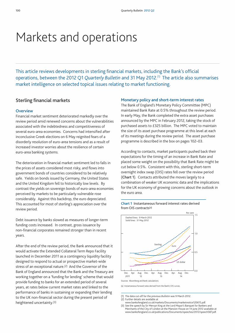
According to contacts, market participants pushed back theirexpectations for the timing of an increase in Bank Rate andplaced some weight on the possibility that Bank Rate might becut below 0.5%. Consistent with this, sterling short-termovernight index swap (OIS) rates fell over the review period(Chart 1). Contacts attributed the moves largely to acombination of weaker UK economic data and the implicationsfor the UK economy of growing concerns about the outlook inthe euro area.
This article reviews developments in sterling financial markets, including the Bank’s officialoperations, between the 2012 Q1 Quarterly Bulletin and 31 May 2012.(1) The article also summarisesmarket intelligence on selected topical issues relating to market functioning.
Markets and operations
(1) The data cut-off for the previous Bulletin was 9 March 2012.(2) Further details are available at
www.bankofengland.co.uk/markets/Documents/marketnotice120615.pdf.(3) See the speech by Sir Mervyn King at the Lord Mayor’s Banquet for Bankers and
Merchants of the City of London at the Mansion House on 14 June 2012 available atwww.bankofengland.co.uk/publications/Documents/speeches/2012/speech587.pdf.
0.0
0.5
1.0
1.5
Dec. Apr. Aug. Dec. Apr. Aug. Dec. Apr. Aug. Dec.
US dollar
Sterling Euro
Dashed lines: 9 March 2012
Solid lines: 31 May 2012
Per cent
12 13 2011 14
Sources: Bloomberg and Bank calculations.
(a) Instantaneous forward rates derived from the Bank’s OIS curves.
Chart 1 Instantaneous forward interest rates derivedfrom OIS contracts(a)
Recent economic and financial developments Markets and operations 101
A Reuters poll released at the end of the review period showedthat a majority of the economists surveyed did not expect the MPC to expand the stock of asset purchases beyond £325 billion. The same poll continued to indicate that themedian expectation was for no increase in Bank Rate over theperiod covered by the survey, which ended in 2013 Q4.
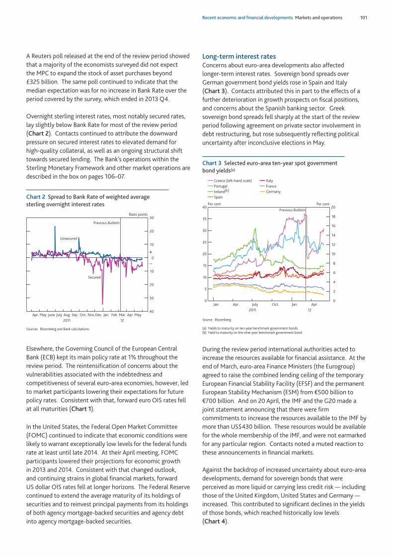
Overnight sterling interest rates, most notably secured rates,lay slightly below Bank Rate for most of the review period(Chart 2). Contacts continued to attribute the downwardpressure on secured interest rates to elevated demand forhigh-quality collateral, as well as an ongoing structural shifttowards secured lending. The Bank’s operations within theSterling Monetary Framework and other market operations aredescribed in the box on pages 106–07.
Elsewhere, the Governing Council of the European CentralBank (ECB) kept its main policy rate at 1% throughout thereview period. The reintensification of concerns about thevulnerabilities associated with the indebtedness andcompetitiveness of several euro-area economies, however, ledto market participants lowering their expectations for futurepolicy rates. Consistent with that, forward euro OIS rates fellat all maturities (Chart 1).
In the United States, the Federal Open Market Committee(FOMC) continued to indicate that economic conditions werelikely to warrant exceptionally low levels for the federal fundsrate at least until late 2014. At their April meeting, FOMCparticipants lowered their projections for economic growth in 2013 and 2014. Consistent with that changed outlook, and continuing strains in global financial markets, forward US dollar OIS rates fell at longer horizons. The Federal Reservecontinued to extend the average maturity of its holdings ofsecurities and to reinvest principal payments from its holdingsof both agency mortgage-backed securities and agency debtinto agency mortgage-backed securities.
Long-term interest ratesConcerns about euro-area developments also affected longer-term interest rates. Sovereign bond spreads overGerman government bond yields rose in Spain and Italy (Chart 3). Contacts attributed this in part to the effects of afurther deterioration in growth prospects on fiscal positions,and concerns about the Spanish banking sector. Greeksovereign bond spreads fell sharply at the start of the reviewperiod following agreement on private sector involvement indebt restructuring, but rose subsequently reflecting politicaluncertainty after inconclusive elections in May.
During the review period international authorities acted toincrease the resources available for financial assistance. At theend of March, euro-area Finance Ministers (the Eurogroup)agreed to raise the combined lending ceiling of the temporaryEuropean Financial Stability Facility (EFSF) and the permanentEuropean Stability Mechanism (ESM) from €500 billion to€700 billion. And on 20 April, the IMF and the G20 made ajoint statement announcing that there were firmcommitments to increase the resources available to the IMF bymore than US$430 billion. These resources would be availablefor the whole membership of the IMF, and were not earmarkedfor any particular region. Contacts noted a muted reaction tothese announcements in financial markets.
Against the backdrop of increased uncertainty about euro-areadevelopments, demand for sovereign bonds that wereperceived as more liquid or carrying less credit risk — includingthose of the United Kingdom, United States and Germany —increased. This contributed to significant declines in the yieldsof those bonds, which reached historically low levels (Chart 4).
0
2
4
6
8
10
12
14
16
18
20
0
5
10
15
20
25
30
35
40
Jan. Apr. July Oct. Jan. Apr.
Per centPer cent
Previous Bulletin
2011 12
Portugal
Ireland(b)
Spain
Italy
France
Germany
Greece (left-hand scale)
Source: Bloomberg.
(a) Yields to maturity on ten-year benchmark government bonds.(b) Yield to maturity on the nine-year benchmark government bond.
Chart 3 Selected euro-area ten-year spot governmentbond yields(a)
40
30
20
10
0
10
20
30
Apr. May June July Aug. Sep. Oct. Nov. Dec. Jan. Feb. Mar. Apr. May
Basis points
2011 12
Secured
Unsecured
Previous Bulletin
+
–
Sources: Bloomberg and Bank calculations.
Chart 2 Spread to Bank Rate of weighted averagesterling overnight interest rates
102 Quarterly Bulletin 2012 Q2
Asset purchases(1)
During the review period, the Bank completed the purchases of gilts mandated by the Monetary Policy Committee (MPC) in February 2012 to increase the size of the programme from£275 billion to £325 billion.(2) The MPC voted to maintain thesize of the asset purchase programme, financed by theissuance of central bank reserves, at £325 billion at each of itsmeetings during the review period.
Purchases of high-quality private sector assets financed by theissuance of Treasury bills and the Debt Management Office’s(DMO’s) cash management operations continued, in line withthe arrangements announced on 29 January 2009.(3)
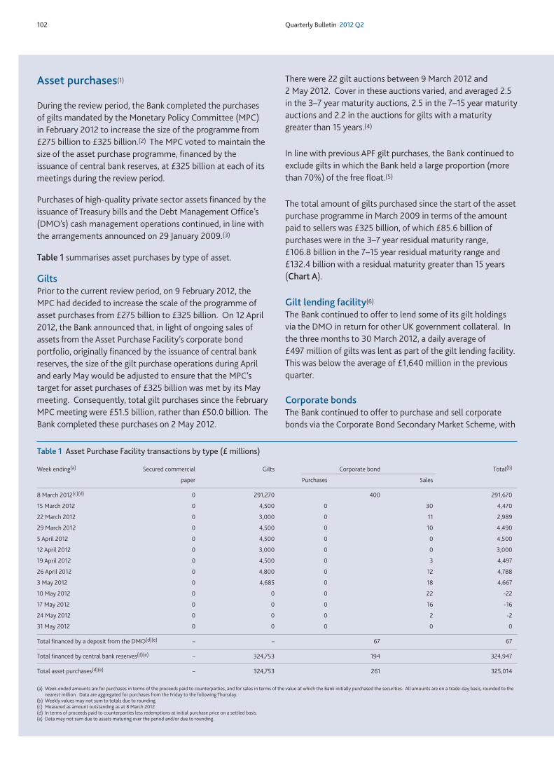
Table 1 summarises asset purchases by type of asset.
GiltsPrior to the current review period, on 9 February 2012, theMPC had decided to increase the scale of the programme ofasset purchases from £275 billion to £325 billion. On 12 April2012, the Bank announced that, in light of ongoing sales ofassets from the Asset Purchase Facility’s corporate bondportfolio, originally financed by the issuance of central bankreserves, the size of the gilt purchase operations during Apriland early May would be adjusted to ensure that the MPC’starget for asset purchases of £325 billion was met by its Maymeeting. Consequently, total gilt purchases since the FebruaryMPC meeting were £51.5 billion, rather than £50.0 billion. TheBank completed these purchases on 2 May 2012.
There were 22 gilt auctions between 9 March 2012 and 2 May 2012. Cover in these auctions varied, and averaged 2.5in the 3–7 year maturity auctions, 2.5 in the 7–15 year maturityauctions and 2.2 in the auctions for gilts with a maturitygreater than 15 years.(4)
In line with previous APF gilt purchases, the Bank continued toexclude gilts in which the Bank held a large proportion (morethan 70%) of the free float.(5)
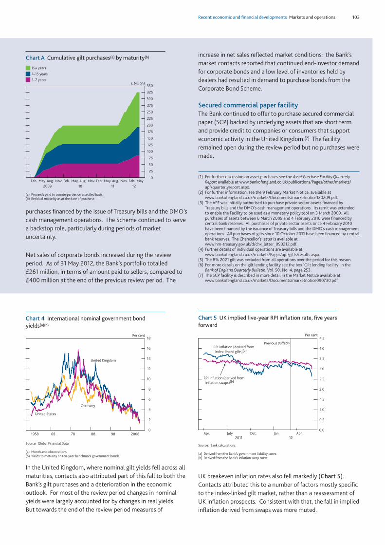
The total amount of gilts purchased since the start of the assetpurchase programme in March 2009 in terms of the amountpaid to sellers was £325 billion, of which £85.6 billion ofpurchases were in the 3–7 year residual maturity range, £106.8 billion in the 7–15 year residual maturity range and£132.4 billion with a residual maturity greater than 15 years(Chart A).
Gilt lending facility(6)
The Bank continued to offer to lend some of its gilt holdingsvia the DMO in return for other UK government collateral. Inthe three months to 30 March 2012, a daily average of £497 million of gilts was lent as part of the gilt lending facility.This was below the average of £1,640 million in the previousquarter.
Corporate bondsThe Bank continued to offer to purchase and sell corporatebonds via the Corporate Bond Secondary Market Scheme, with
Table 1 Asset Purchase Facility transactions by type (£ millions)
Week ending(a) Secured commercial Gilts Corporate bond Total(b)
paper Purchases Sales
8 March 2012(c)(d) 0 291,270 400 291,670
15 March 2012 0 4,500 0 30 4,470
22 March 2012 0 3,000 0 11 2,989
29 March 2012 0 4,500 0 10 4,490
5 April 2012 0 4,500 0 0 4,500
12 April 2012 0 3,000 0 0 3,000
19 April 2012 0 4,500 0 3 4,497
26 April 2012 0 4,800 0 12 4,788
3 May 2012 0 4,685 0 18 4,667
10 May 2012 0 0 0 22 -22
17 May 2012 0 0 0 16 -16
24 May 2012 0 0 0 2 -2
31 May 2012 0 0 0 0 0
Total financed by a deposit from the DMO(d)(e) – – 67 67
Total financed by central bank reserves(d)(e) – 324,753 194 324,947
Total asset purchases(d)(e) – 324,753 261 325,014
(a) Week-ended amounts are for purchases in terms of the proceeds paid to counterparties, and for sales in terms of the value at which the Bank initially purchased the securities. All amounts are on a trade-day basis, rounded to thenearest million. Data are aggregated for purchases from the Friday to the following Thursday.
(b) Weekly values may not sum to totals due to rounding.(c) Measured as amount outstanding as at 8 March 2012.(d) In terms of proceeds paid to counterparties less redemptions at initial purchase price on a settled basis.(e) Data may not sum due to assets maturing over the period and/or due to rounding.
Recent economic and financial developments Markets and operations 103
In the United Kingdom, where nominal gilt yields fell across allmaturities, contacts also attributed part of this fall to both theBank’s gilt purchases and a deterioration in the economicoutlook. For most of the review period changes in nominalyields were largely accounted for by changes in real yields. But towards the end of the review period measures of
UK breakeven inflation rates also fell markedly (Chart 5).Contacts attributed this to a number of factors mostly specificto the index-linked gilt market, rather than a reassessment ofUK inflation prospects. Consistent with that, the fall in impliedinflation derived from swaps was more muted.
0
2
4
6
8
10
12
14
16
18
1958 68 78 88 98 2008
Germany
United Kingdom
United States
Per cent
Source: Global Financial Data.
(a) Month-end observations.(b) Yields to maturity on ten-year benchmark government bonds.
Chart 4 International nominal government bondyields(a)(b)
0.0
0.5
1.0
1.5
2.0
2.5
3.0
3.5
4.0
4.5
Apr. July Oct. Jan. Apr.
Per cent
Previous Bulletin
2011 12
RPI inflation (derived from
index-linked gilts)(a)
RPI inflation (derived from
inflation swaps)(b)
Source: Bank calculations.
(a) Derived from the Bank’s government liability curve.(b) Derived from the Bank’s inflation swap curve.
Chart 5 UK implied five-year RPI inflation rate, five yearsforward
purchases financed by the issue of Treasury bills and the DMO’scash management operations. The Scheme continued to servea backstop role, particularly during periods of marketuncertainty.
Net sales of corporate bonds increased during the reviewperiod. As of 31 May 2012, the Bank’s portfolio totalled £261 million, in terms of amount paid to sellers, compared to£400 million at the end of the previous review period. The
increase in net sales reflected market conditions: the Bank’smarket contacts reported that continued end-investor demandfor corporate bonds and a low level of inventories held bydealers had resulted in demand to purchase bonds from theCorporate Bond Scheme.
Secured commercial paper facilityThe Bank continued to offer to purchase secured commercialpaper (SCP) backed by underlying assets that are short termand provide credit to companies or consumers that supporteconomic activity in the United Kingdom.(7) The facilityremained open during the review period but no purchases weremade.
0
25
50
75
100
125
150
175
200
225
250
275
300
325
350
Feb. May Aug. Nov. Feb. May Aug. Nov. Feb. May Aug. Nov. Feb. May
15+ years
7–15 years
3–7 years£ billions
2009 10 11 12
(a) Proceeds paid to counterparties on a settled basis.(b) Residual maturity as at the date of purchase.
Chart A Cumulative gilt purchases(a) by maturity(b)
(1) For further discussion on asset purchases see the Asset Purchase Facility QuarterlyReport available at www.bankofengland.co.uk/publications/Pages/other/markets/apf/quarterlyreport.aspx.
(2) For further information, see the 9 February Market Notice, available atwww.bankofengland.co.uk/markets/Documents/marketnotice120209.pdf.
(3) The APF was initially authorised to purchase private sector assets financed by Treasury bills and the DMO’s cash management operations. Its remit was extended to enable the Facility to be used as a monetary policy tool on 3 March 2009. Allpurchases of assets between 6 March 2009 and 4 February 2010 were financed bycentral bank reserves. All purchases of private sector assets since 4 February 2010have been financed by the issuance of Treasury bills and the DMO’s cash managementoperations. All purchases of gilts since 10 October 2011 have been financed by centralbank reserves. The Chancellor’s letter is available at www.hm-treasury.gov.uk/d/chx_letter_090212.pdf.
(4) Further details of individual operations are available atwww.bankofengland.co.uk/markets/Pages/apf/gilts/results.aspx.
(5) The 8% 2021 gilt was excluded from all operations over the period for this reason.(6) For more details on the gilt lending facility see the box ‘Gilt lending facility’ in the
Bank of England Quarterly Bulletin, Vol. 50, No. 4, page 253.(7) The SCP facility is described in more detail in the Market Notice available at
www.bankofengland.co.uk/markets/Documents/marketnotice090730.pdf.
104 Quarterly Bulletin 2012 Q2
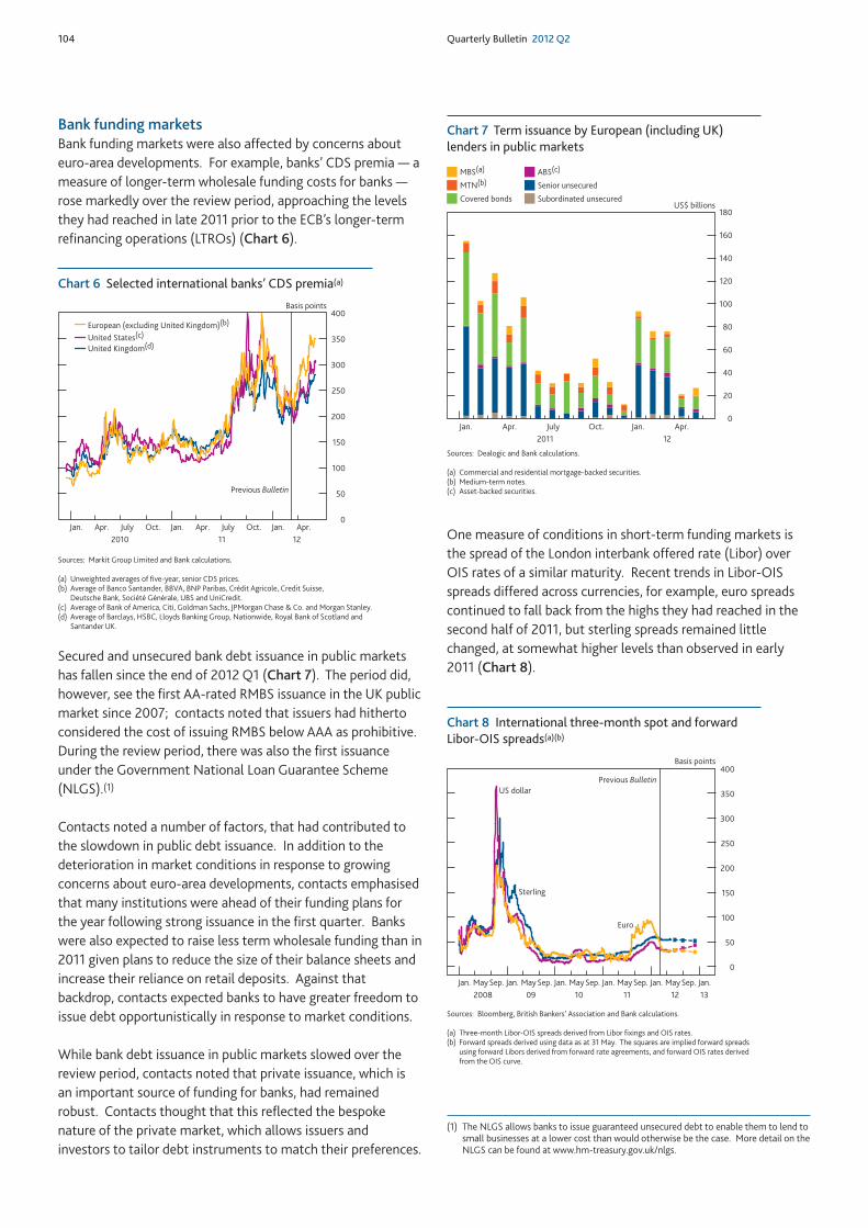
Bank funding marketsBank funding markets were also affected by concerns abouteuro-area developments. For example, banks’ CDS premia — ameasure of longer-term wholesale funding costs for banks —rose markedly over the review period, approaching the levelsthey had reached in late 2011 prior to the ECB’s longer-termrefinancing operations (LTROs) (Chart 6).
Secured and unsecured bank debt issuance in public marketshas fallen since the end of 2012 Q1 (Chart 7). The period did,however, see the first AA-rated RMBS issuance in the UK publicmarket since 2007; contacts noted that issuers had hithertoconsidered the cost of issuing RMBS below AAA as prohibitive.During the review period, there was also the first issuanceunder the Government National Loan Guarantee Scheme(NLGS).(1)
Contacts noted a number of factors, that had contributed tothe slowdown in public debt issuance. In addition to thedeterioration in market conditions in response to growingconcerns about euro-area developments, contacts emphasisedthat many institutions were ahead of their funding plans forthe year following strong issuance in the first quarter. Bankswere also expected to raise less term wholesale funding than in2011 given plans to reduce the size of their balance sheets andincrease their reliance on retail deposits. Against thatbackdrop, contacts expected banks to have greater freedom toissue debt opportunistically in response to market conditions.
While bank debt issuance in public markets slowed over thereview period, contacts noted that private issuance, which isan important source of funding for banks, had remainedrobust. Contacts thought that this reflected the bespokenature of the private market, which allows issuers andinvestors to tailor debt instruments to match their preferences.
One measure of conditions in short-term funding markets isthe spread of the London interbank offered rate (Libor) overOIS rates of a similar maturity. Recent trends in Libor-OISspreads differed across currencies, for example, euro spreadscontinued to fall back from the highs they had reached in thesecond half of 2011, but sterling spreads remained littlechanged, at somewhat higher levels than observed in early2011 (Chart 8).
0
50
100
150
200
250
300
350
400
Jan. Apr. July Oct. Jan. Apr. July Oct. Jan. Apr.
Basis points
2010 11 12
Previous Bulletin
United Kingdom(d) United States(c) European (excluding United Kingdom)(b)
Sources: Markit Group Limited and Bank calculations.
(a) Unweighted averages of five-year, senior CDS prices.(b) Average of Banco Santander, BBVA, BNP Paribas, Crédit Agricole, Credit Suisse,
Deutsche Bank, Société Générale, UBS and UniCredit.(c) Average of Bank of America, Citi, Goldman Sachs, JPMorgan Chase & Co. and Morgan Stanley.(d) Average of Barclays, HSBC, Lloyds Banking Group, Nationwide, Royal Bank of Scotland and
Santander UK.
Chart 6 Selected international banks’ CDS premia(a)
0
20
40
60
80
100
120
140
160
180
Jan. Apr. July Oct. Jan. Apr.
Subordinated unsecured
2011 12
US$ billions
MBS(a)
MTN(b)
Covered bonds
ABS(c)
Senior unsecured
Sources: Dealogic and Bank calculations.
(a) Commercial and residential mortgage-backed securities.(b) Medium-term notes.(c) Asset-backed securities.
Chart 7 Term issuance by European (including UK)lenders in public markets
(1) The NLGS allows banks to issue guaranteed unsecured debt to enable them to lend tosmall businesses at a lower cost than would otherwise be the case. More detail on theNLGS can be found at www.hm-treasury.gov.uk/nlgs.
0
50
100
150
200
250
300
350
400
Jan. May Sep. Jan. May Sep. Jan. May Sep. Jan. May Sep. Jan. May Sep. Jan.
Sterling
US dollar
Euro
Basis points
2008
Previous Bulletin
12 1309 10 11
Sources: Bloomberg, British Bankers’ Association and Bank calculations.
(a) Three-month Libor-OIS spreads derived from Libor fixings and OIS rates.(b) Forward spreads derived using data as at 31 May. The squares are implied forward spreads
using forward Libors derived from forward rate agreements, and forward OIS rates derivedfrom the OIS curve.
Chart 8 International three-month spot and forwardLibor-OIS spreads(a)(b)
Recent economic and financial developments Markets and operations 105
Contacts cited a number of possible explanations for thedivergence between sterling and euro Libor-OIS spreads. Inparticular, contacts pointed to the impact of the ECB’s twoLTROs, which had markedly increased the supply of euros inthe market. But the subdued volume of interbank lending inthe sterling market was also thought to be a factor. Inaddition, pricing in foreign exchange swap markets impliedthat banks that could borrow in either euro or sterling facedsimilar short-term unsecured funding costs in either currency.Nonetheless, contacts recognised that these factors may notprovide a full explanation for the persistently elevated level ofsterling Libor-OIS spreads.
On 15 June 2012, after the end of the review period, the Bank announced that it would activate the Extended CollateralTerm Repo Facility, providing sterling liquidity with a term ofsix months against collateral pre-positioned for use in theBank’s Discount Window Facility. The minimum bid rate inthese auctions would be a spread to Bank Rate of 25 basis points. The first operation would be held on 20 June 2012.(1) Immediately following the announcement,forward sterling Libor-OIS spreads fell.
Conditions in short-term US dollar funding markets forEuropean banks improved a little further: the differencebetween the cost of raising US dollar funding by borrowing ineuro and swapping via the foreign exchange market and thecost of direct US dollar borrowing fell by 10 basis points.
During the review period, credit rating agencies downgraded anumber of bank ratings. Many of these downgrades were partof Moody’s previously announced banking sector review. Theimmediate response in financial markets was relatively muted.Contacts thought this in part reflected the fact that Moody’sreviews had been pre-announced, banks had taken mitigatingactions and that some investors and asset managers wereexpected to respond to the downgrades by adapting theirinternal ratings criteria.
At the end of the review period, Moody’s review of banks withglobal capital market operations, which included several UK and US banks, had not been concluded.
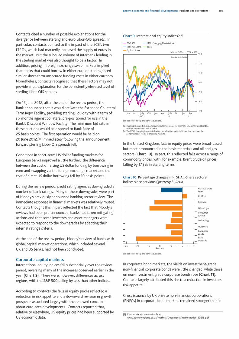
Corporate capital marketsInternational equity indices fell substantially over the reviewperiod, reversing many of the increases observed earlier in theyear (Chart 9). There were, however, differences acrossregions, with the S&P 500 falling by less than other indices.
According to contacts the falls in equity prices reflected areduction in risk appetite and a downward revision in growthprospects associated largely with the renewed concerns about euro-area developments. Contacts reported that,relative to elsewhere, US equity prices had been supported byUS economic data.
In the United Kingdom, falls in equity prices were broad-based,but most pronounced in the basic materials and oil and gassectors (Chart 10). In part, this reflected falls across a range ofcommodity prices, with, for example, Brent crude oil pricesfalling by 17.3% in sterling terms.
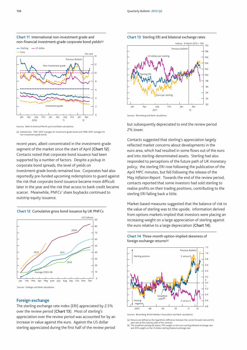
In corporate bond markets, the yields on investment-gradenon-financial corporate bonds were little changed, while thoseon non-investment grade corporate bonds rose (Chart 11).Contacts largely attributed this rise to a reduction in investors’risk appetite.
Gross issuance by UK private non-financial corporations(PNFCs) in corporate bond markets remained stronger than in
25 20 15 10 5 0 5
Consumer
goods
Technology
Basic
materials
Industrials
Consumer
services
Oil and gas
Utilities
Financials
FTSE All-Share
index
Per cent+–
Sources: Bloomberg and Bank calculations.
Chart 10 Percentage changes in FTSE All-Share sectoralindices since previous Quarterly Bulletin
Chart 9 International equity indices(a)(b)
70
80
90
100
110
120
130
Jan. Apr. July Oct. Jan. Apr. July Oct. Jan. Apr.
S&P 500
Topix
DJ Euro Stoxx
MSCI Emerging Markets index
FTSE All-Share
2010
Previous Bulletin
Indices: 9 March 2012 = 100
11 12
Sources: Bloomberg and Bank calculations.
(a) Indices are quoted in domestic currency terms, except for the MSCI Emerging Markets index,which is quoted in US dollar terms.
(b) The MSCI Emerging Markets index is a capitalisation-weighted index that monitors theperformance of stocks in emerging markets.
(1) Further details are available atwww.bankofengland.co.uk/markets/Documents/marketnotice120615.pdf.
106 Quarterly Bulletin 2012 Q2
Operations within the Sterling MonetaryFramework and other market operations
The level of central bank reserves continued to be determinedby (i) the stock of reserves injected via the Asset PurchaseFacility (APF), (ii) the level of reserves supplied by long-termrepo open market operations (OMOs) and (iii) the net impactof other sterling (‘autonomous factor’) flows across the Bank’sbalance sheet. This box describes the Bank’s operations withinthe Sterling Monetary Framework over the review period, andother market operations. The box on pages 102–03 providesmore detail on the APF.
Operational Standing FacilitiesSince 5 March 2009, the rate paid on the Operational StandingDeposit Facility has been zero, while all reserves accountbalances have been remunerated at Bank Rate. Reflecting this,average use of the deposit facility was £0 million in each of themaintenance periods under review. Average use of the lendingfacility was also £0 million throughout the period.
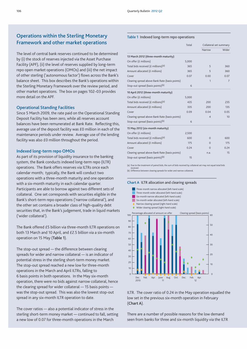
Indexed long-term repo OMOsAs part of its provision of liquidity insurance to the bankingsystem, the Bank conducts indexed long-term repo (ILTR)operations. The Bank offers reserves via ILTRs once eachcalendar month; typically, the Bank will conduct twooperations with a three-month maturity and one operationwith a six-month maturity in each calendar quarter.Participants are able to borrow against two different sets ofcollateral. One set corresponds with securities eligible in theBank’s short-term repo operations (‘narrow collateral’), andthe other set contains a broader class of high-quality debtsecurities that, in the Bank’s judgement, trade in liquid markets(‘wider collateral’).
The Bank offered £5 billion via three-month ILTR operations onboth 13 March and 10 April, and £2.5 billion via a six-monthoperation on 15 May (Table 1).
The stop-out spread — the difference between clearingspreads for wider and narrow collateral — is an indicator ofpotential stress in the sterling short-term money market. The stop-out spread reached a new low for three-monthoperations in the March and April ILTRs, falling to 6 basis points in both operations. In the May six-monthoperation, there were no bids against narrow collateral, hencethe clearing spread for wider collateral — 15 basis points —was the stop-out spread. This was also the lowest stop-outspread in any six-month ILTR operation to date.
The cover ratios — also a potential indicator of stress in thesterling short-term money market — continued to fall, settinga new low of 0.07 for three-month operations in the March
ILTR. The cover ratio of 0.24 in the May operation equalled thelow set in the previous six-month operation in February (Chart A).
There are a number of possible reasons for the low demandseen from banks for three and six-month liquidity via the ILTR
Table 1 Indexed long-term repo operations
Total Collateral set summary
Narrow Wider
13 March 2012 (three-month maturity)
On offer (£ millions) 5,000
Total bids received (£ millions)(a) 365 5 360
Amount allocated (£ millions) 365 5 360
Cover 0.07 0.00 0.07
Clearing spread above Bank Rate (basis points) 1 7
Stop-out spread (basis points)(b) 6
10 April 2012 (three-month maturity)
On offer (£ millions) 5,000
Total bids received (£ millions)(a) 435 200 235
Amount allocated (£ millions) 335 200 135
Cover 0.09 0.04 0.05
Clearing spread above Bank Rate (basis points) 4 10
Stop-out spread (basis points)(b) 6
15 May 2012 (six-month maturity)
On offer (£ millions) 2,500
Total bids received (£ millions)(a) 600 0 600
Amount allocated (£ millions) 175 0 175
Cover 0.24 0 0.24
Clearing spread above Bank Rate (basis points) n.a. 15
Stop-out spread (basis points)(b) 15
(a) Due to the treatment of paired bids, the sum of bids received by collateral set may not equal total bidsreceived.
(b) Difference between clearing spreads for wider and narrow collateral.
0
10
20
30
40
50
60
0
10
20
30
40
50
60
70
80
90
100
Dec. Feb. Apr. June Aug. Oct. Dec. Feb. Apr.
Three-month narrow allocated (left-hand scale)
Three-month wider allocated (left-hand scale)
Six-month narrow allocated (left-hand scale)
Six-month wider allocated (left-hand scale)
Narrow clearing spread (right-hand scale)
Wider clearing spread (right-hand scale)
Percentage allocated of amount on offer Clearing spread (basis points)
2010 11 12
Chart A ILTR allocation and clearing spreads
Recent economic and financial developments Markets and operations 107
operations. First, short-term secured market interest ratesremain below Bank Rate, making repo markets a potentiallycheaper source of liquidity. Second, the APF asset purchaseprogramme and the ECB’s three-year longer-term refinancingoperations (LTROs) supplied liquidity to the banking system,which may have reduced the need for counterparties to usethe ILTR operations to meet their short-term liquidity needs.
Reserves provided via ILTRs during the review period weremore than offset by the maturity of loans provided in previousILTR operations. Consequently, the stock of liquidity providedthrough these operations declined.
Discount Window FacilityThe Discount Window Facility (DWF) provides liquidityinsurance to the banking system by allowing eligible banks to borrow gilts against a wide range of collateral. On 3 April 2012, the Bank announced that the average dailyamount outstanding in the DWF between 1 October and 31 December 2011, lent with a maturity of 30 days or less, was£0 million. The Bank also announced that the average dailyamount outstanding in the DWF between 1 October and 31 December 2010, lent with a maturity of more than 30 days,was £0 million.
The Bank encourages banks to pre-position collateral forpotential use in the DWF, so that there would not be a need toassess the collateral at short notice in the event of a suddenand unexpected request to borrow from the DWF. The Bankreported that banks had pre-positioned collateral with a totallendable value of around £160 billion in the DWF as of 29 March 2012.(1)
Extended Collateral Term Repo FacilityThe Extended Collateral Term Repo Facility is a contingentliquidity facility, designed to mitigate risks to financial stabilityarising from a market-wide shortage of short-term sterlingliquidity.(2) As of 31 May 2012, no operations under the Facilityhad been announced.
Other operationsUS dollar repo operationsOn 11 May 2010, the Bank reintroduced weekly fixed-ratetenders with a seven-day maturity to offer US dollar liquidity,in co-ordination with other central banks, in response torenewed strains in the short-term funding market for US dollars. As of 31 May 2012, there had been no use of theBank’s facility.
On 30 November 2011, the Bank announced, in co-ordinationwith the Bank of Canada, the Bank of Japan, the ECB, the Swiss National Bank, and the Federal Reserve, that theauthorisation of the existing temporary US dollar swap
arrangements had been extended to 1 February 2013, that 84-day US dollar tenders would continue until this time, and that seven-day operations would continue until furthernotice. It also announced that the central banks had agreed tolower the pricing on the US dollar swap arrangements by 50 basis points to the US dollar overnight index swap rate plus50 basis points. As a contingency measure, the six centralbanks agreed to establish a network of temporary bilateralliquidity swap arrangements that will be available until 1 February 2013.
Bank of England balance sheet: capital portfolioThe Bank holds an investment portfolio that is approximatelythe same size as its capital and reserves (net of equityholdings, for example in the Bank for InternationalSettlements, and the Bank’s physical assets) and aggregatecash ratio deposits. The portfolio consists of sterling-denominated securities. Securities purchased by theBank for this portfolio are normally held to maturity;nevertheless sales may be made from time to time, reflectingfor example, risk management, liquidity management orchanges in investment policy.
The portfolio currently includes around £3.5 billion of gilts and£0.4 billion of other debt securities. Over the review period,gilt purchases were made in accordance with the quarterlyannouncements on 3 January and 2 April 2012.
(1) See the speech by Paul Fisher, ‘Liquidity support from the Bank of England: theDiscount Window Facility’, 29 March 2012, available atwww.bankofengland.co.uk/publications/Documents/speeches/2012/speech561.pdf.
(2) Further details are available atwww.bankofengland.co.uk/markets/Pages/money/ectr/index.aspx.
108 Quarterly Bulletin 2012 Q2
recent years, albeit concentrated in the investment-gradesegment of the market since the start of April (Chart 12).Contacts noted that corporate bond issuance had beensupported by a number of factors. Despite a pickup incorporate bond spreads, the level of yields on investment-grade bonds remained low. Corporates had alsoreportedly pre-funded upcoming redemptions to guard againstthe risk that corporate bond issuance became more difficultlater in the year and the risk that access to bank credit becamescarcer. Meanwhile, PNFCs’ share buybacks continued tooutstrip equity issuance.
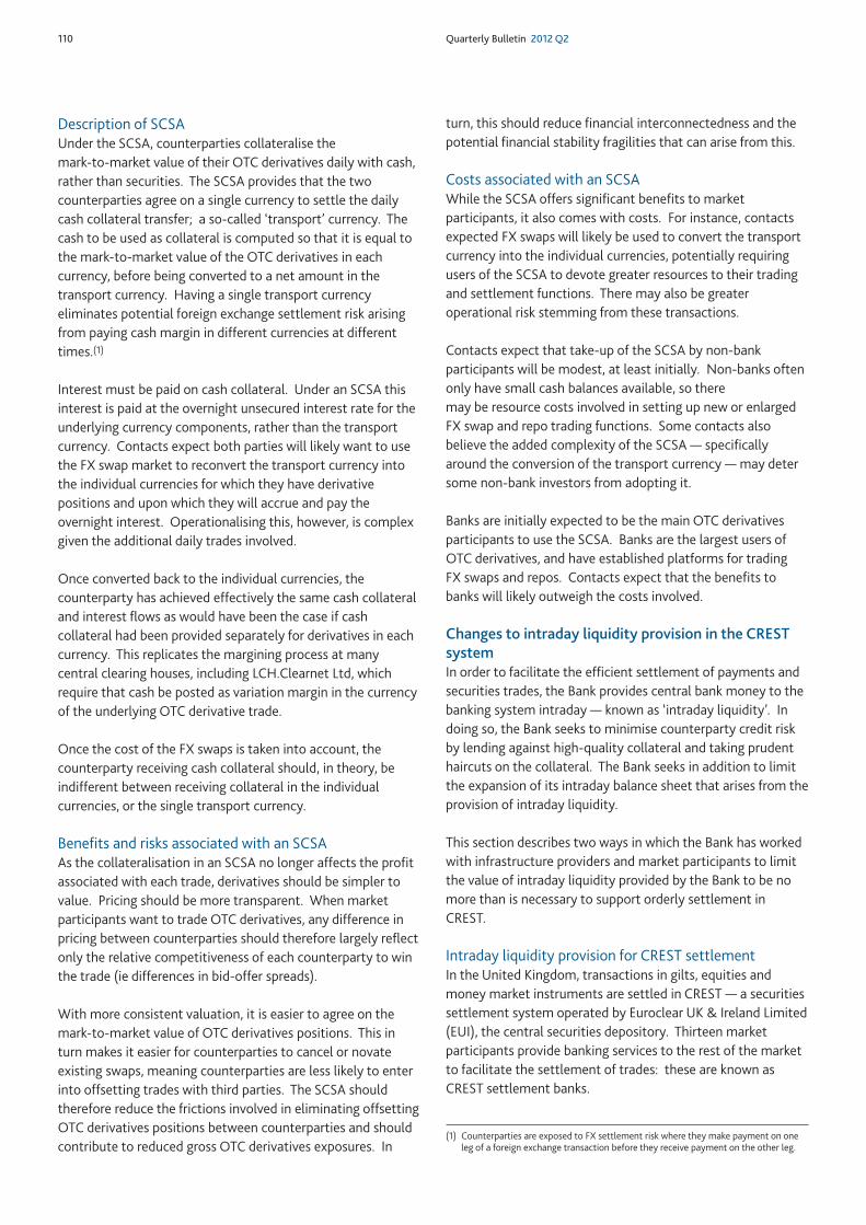
Foreign exchangeThe sterling exchange rate index (ERI) appreciated by 2.5%over the review period (Chart 13). Most of sterling’sappreciation over the review period was accounted for by anincrease in value against the euro. Against the US dollarsterling appreciated during the first half of the review period
but subsequently depreciated to end the review period 2% lower.
Contacts suggested that sterling’s appreciation largelyreflected market concerns about developments in the euro area, which had resulted in some flows out of the euroand into sterling-denominated assets. Sterling had alsoresponded to perceptions of the future path of UK monetarypolicy; the sterling ERI rose following the publication of theApril MPC minutes, but fell following the release of the May Inflation Report. Towards the end of the review period,contacts reported that some investors had sold sterling torealise profits on their trading positions, contributing to thesterling ERI falling back a little.
Market-based measures suggested that the balance of risk tothe value of sterling was to the upside; information derivedfrom options markets implied that investors were placing anincreasing weight on a large appreciation of sterling againstthe euro relative to a large depreciation (Chart 14).
90
92
94
96
98
100
102
104
106
108
110
Jan. Apr. July Oct. Jan. Apr.
Indices: 9 March 2012 = 100
Previous Bulletin
2011 12
US dollars per sterling
Euro per sterling
Sterling ERI
Sources: Bloomberg and Bank calculations.
Chart 13 Sterling ERI and bilateral exchange rates
0.8
0.6
0.4
0.2
0.0
0.2
0.4
0.6
0.8
1.0
1.2
08 09 10 11 122007
Sterling positive
Sterling
negative
Previous Bulletin
£ versus €
Simplified £ERI(b)
£ versus $
+
–
Sources: Bloomberg, British Bankers’ Association and Bank calculations.
(a) Returns are defined as the logarithmic difference between the current forward rate and thespot rate at the maturity date of the contract.
(b) The simplified sterling ERI places 70% weight on the euro-sterling bilateral exchange rateand 30% weight on the US dollar-sterling bilateral exchange rate.
Chart 14 Three-month option-implied skewness offoreign exchange returns(a)
0
10
20
30
40
50
60
70
80
90
Jan. Feb. Mar. Apr. May June July Aug. Sep. Oct. Nov. Dec.
US$ billions
2009
Average 2003–08
2010
2011 2012
Sources: Dealogic and Bank calculations.
Chart 12 Cumulative gross bond issuance by UK PNFCs
0
2
4
6
8
10
12
14
Jan. Apr. July Oct. Jan. Apr. July Oct. Jan. Apr.
Non-investment grade
Investment grade
2010 11 12
Per cent
Previous Bulletin
US dollar
Euro
Sterling
Sources: Bank of America/Merrill Lynch and Bank calculations.
(a) Dashed lines: 1997–2007 averages for investment-grade bonds and 1998–2007 averages fornon-investment grade bonds.
Chart 11 International non-investment grade andnon-financial investment-grade corporate bond yields(a)

Recent economic and financial developments Markets and operations 109
Developments in market structure
This section describes two recent developments in marketstructure. First, it describes the development of StandardisedCredit Support Annexes used in over-the-counter derivativestransactions, using market intelligence gathered from a widerange of contacts. And second, it describes recent changes tointraday liquidity provision by the Bank of England in theCREST system.
Standardised Credit Support AnnexesCredit Support Annexes (CSAs) relate to derivatives contractsthat are agreed and settled bilaterally between twocounterparties (rather than via an exchange or tradingplatform). Such over-the-counter (OTC) derivatives make upthe majority of derivatives trades between banks and end-users, such as corporates and asset managers.
Over time, the value of a derivative trade will change as, forexample, market prices change. This creates a so-called mark-to-market gain or loss and exposes the counterpartywith a positive mark-to-market position to counterparty creditrisk. Such counterparty credit risk is usually managed viacollateralisation of the mark-to-market position.(1) Thisrequires regular flows of collateral between the twocounterparties depending on how the mark-to-market positionchanges — this is known as margining.
The rules around collateralising OTC derivatives are set outwithin the CSA which forms part of the International Swapsand Derivatives Association (ISDA) Master Agreement definingthe trading relationship between two counterparties. Theprimary purpose of CSAs is to mitigate counterparty credit risk,through collateralisation. This section describes CSAs, and theremaining challenges a Standardised CSA (SCSA) is designed toaddress.
Role of CSAsCSAs outline:
• The type of collateral that each counterparty can provide assecurity to cover the net mark-to-market position of OTCderivatives.
• How frequently positions are margined.• Whether thresholds exist for calling additional margin
collateral.
Contacts note that there are a wide variety of CSAs inexistence because they are negotiated bilaterally betweenindividual counterparties and are tailored to suit specificrequirements; often particular to the time the CSA wasagreed.(2) In many cases, CSAs give the counterparty that hasa negative mark-to-market value the option to choose whichcollateral to deliver from a defined list of several types ofcollateral.
Challenges with current CSAsCounterparties are not indifferent when it comes to whatcollateral they receive. Consequently, the range of collateraldefined in the CSA can affect the valuation of OTC derivatives.For example, when a bank trades an interest rate swap with aclient it will normally enter into an offsetting trade in theinterbank market, to hedge its market risk. This offsettingtrade would also usually be subject to a collateralisationagreement. If the interest rate swap has positive mark-to-market value for the bank, the client will have toprovide collateral as set out in the CSA. The bank can typicallyuse the collateral it receives from the client to collateralise theoffsetting trade, which should have a negative mark-to-marketvalue.
If the collateral on the two trades match, the bank has noadditional costs of trading. But if the CSA allows the client topost collateral that the bank cannot use to collateralise itsoffsetting trade, the bank would need to use repo and/or FX swap markets to convert the collateral received into thecollateral it is allowed to deliver.(3) This can change the bank’sexpected profit and loss, and hence the value of the swap.
Where optionality to provide different types of collateral existsit creates uncertainty about the future profit and loss. Thisuncertainty is most significant where there is an option toprovide collateral in different currencies. Estimating the valueof this optionality is very complex. It involves forecasting theexpected future mark-to-market value of the swap, whichcollateral will likely be delivered at different points in time, andthe estimated future costs of converting collateral in repoand/or FX swap markets.
According to contacts, some banks have tried to address thisproblem by charging clients for this collateral option. Butdifferences in assumptions and pricing methodology meanthat OTC derivatives with different CSAs are not always pricedconsistently by market participants. This can lead to disputesabout the valuation of derivatives, and consequently make itmore difficult to cancel a trade or find an external party to‘step in’ and take the client’s place at an agreed price — so-called ‘novation’. Where counterparties cannot agree avalue to cancel or novate existing derivatives, they may tradenew, offsetting swaps with other counterparties instead. Thisincreases the interconnectedness of the financial system.
A formal industry initiative to deal with the valuation problemscreated by collateral optionality is under way through ISDA’sproposed SCSA.
(1) ISDA undertakes an annual survey providing information on the use of collateral in theOTC derivatives market. Surveys can be found at www2.isda.org/functional-areas/research/surveys/margin-surveys.
(2) CSAs are not always symmetric; in some cases, only one of the counterparties isrequired to post collateral on positions that are out-of-the-money, so-called one-wayCSAs.
(3) Alternatively, the bank could use other CSA-eligible collateral it has available on itsbalance sheet. But this has an opportunity cost, as that collateral cannot therefore beused for other purposes.
Description of SCSAUnder the SCSA, counterparties collateralise the mark-to-market value of their OTC derivatives daily with cash,rather than securities. The SCSA provides that the twocounterparties agree on a single currency to settle the dailycash collateral transfer; a so-called ‘transport’ currency. Thecash to be used as collateral is computed so that it is equal tothe mark-to-market value of the OTC derivatives in eachcurrency, before being converted to a net amount in thetransport currency. Having a single transport currencyeliminates potential foreign exchange settlement risk arisingfrom paying cash margin in different currencies at differenttimes.(1)
Interest must be paid on cash collateral. Under an SCSA thisinterest is paid at the overnight unsecured interest rate for theunderlying currency components, rather than the transportcurrency. Contacts expect both parties will likely want to usethe FX swap market to reconvert the transport currency intothe individual currencies for which they have derivativepositions and upon which they will accrue and pay theovernight interest. Operationalising this, however, is complexgiven the additional daily trades involved.
Once converted back to the individual currencies, thecounterparty has achieved effectively the same cash collateraland interest flows as would have been the case if cashcollateral had been provided separately for derivatives in eachcurrency. This replicates the margining process at manycentral clearing houses, including LCH.Clearnet Ltd, whichrequire that cash be posted as variation margin in the currencyof the underlying OTC derivative trade.
Once the cost of the FX swaps is taken into account, thecounterparty receiving cash collateral should, in theory, beindifferent between receiving collateral in the individualcurrencies, or the single transport currency.
Benefits and risks associated with an SCSAAs the collateralisation in an SCSA no longer affects the profitassociated with each trade, derivatives should be simpler tovalue. Pricing should be more transparent. When marketparticipants want to trade OTC derivatives, any difference inpricing between counterparties should therefore largely reflectonly the relative competitiveness of each counterparty to winthe trade (ie differences in bid-offer spreads).
With more consistent valuation, it is easier to agree on themark-to-market value of OTC derivatives positions. This inturn makes it easier for counterparties to cancel or novateexisting swaps, meaning counterparties are less likely to enterinto offsetting trades with third parties. The SCSA shouldtherefore reduce the frictions involved in eliminating offsettingOTC derivatives positions between counterparties and shouldcontribute to reduced gross OTC derivatives exposures. In
turn, this should reduce financial interconnectedness and thepotential financial stability fragilities that can arise from this.
Costs associated with an SCSAWhile the SCSA offers significant benefits to marketparticipants, it also comes with costs. For instance, contactsexpected FX swaps will likely be used to convert the transportcurrency into the individual currencies, potentially requiringusers of the SCSA to devote greater resources to their tradingand settlement functions. There may also be greateroperational risk stemming from these transactions.
Contacts expect that take-up of the SCSA by non-bankparticipants will be modest, at least initially. Non-banks oftenonly have small cash balances available, so there may be resource costs involved in setting up new or enlargedFX swap and repo trading functions. Some contacts alsobelieve the added complexity of the SCSA — specificallyaround the conversion of the transport currency — may detersome non-bank investors from adopting it.
Banks are initially expected to be the main OTC derivativesparticipants to use the SCSA. Banks are the largest users ofOTC derivatives, and have established platforms for trading FX swaps and repos. Contacts expect that the benefits tobanks will likely outweigh the costs involved.
Changes to intraday liquidity provision in the CRESTsystemIn order to facilitate the efficient settlement of payments andsecurities trades, the Bank provides central bank money to thebanking system intraday — known as ‘intraday liquidity’. Indoing so, the Bank seeks to minimise counterparty credit riskby lending against high-quality collateral and taking prudenthaircuts on the collateral. The Bank seeks in addition to limitthe expansion of its intraday balance sheet that arises from theprovision of intraday liquidity.
This section describes two ways in which the Bank has workedwith infrastructure providers and market participants to limitthe value of intraday liquidity provided by the Bank to be nomore than is necessary to support orderly settlement in CREST.
Intraday liquidity provision for CREST settlementIn the United Kingdom, transactions in gilts, equities andmoney market instruments are settled in CREST — a securitiessettlement system operated by Euroclear UK & Ireland Limited(EUI), the central securities depository. Thirteen marketparticipants provide banking services to the rest of the marketto facilitate the settlement of trades: these are known asCREST settlement banks.
110 Quarterly Bulletin 2012 Q2
(1) Counterparties are exposed to FX settlement risk where they make payment on oneleg of a foreign exchange transaction before they receive payment on the other leg.
Recent economic and financial developments Markets and operations 111
Since 2001, CREST settlement has operated on a simultaneousdelivery versus payment (DvP) basis. This means that when aCREST member settles a securities purchase, a simultaneoustransfer of central bank money is made from the purchasingmember’s settlement bank to the selling member’s settlementbank. A CREST settlement bank must have access to centralbank money in CREST intraday, in order to honour thepayment leg of DvP purchase transactions entered into by thatsettlement bank’s clients.
Settlement banks can use central bank money from theirreserves accounts at the Bank to meet these intraday CRESTliquidity needs. Where additional central bank money isrequired in order to settle large DvP payment obligations, theBank is willing to provide intraday liquidity to settlementbanks, in pursuit of its financial stability objective.
The provision of intraday liquidity exposes the Bank tocounterparty credit risk. While intraday liquidity iscollateralised by high-quality assets with prudent haircuts,there is always a residual risk that market prices would movesignificantly at times of stress and the Bank may not be able torecover the full value of a loan in a timely manner in the eventof a counterparty default; this would complicate the Bank’smanagement of its balance sheet.(1)
Such risks are small, but as they are not zero it is prudent forthe Bank to limit the creation of intraday liquidity to no morethan the amount that is required to support orderlysettlement.
Removing the automated oversupply of intraday liquidityThe first way in which intraday liquidity provision is beingoptimised is a recent change to the technical design of theCREST system.
In order to support the settlement of high-value transactionssuch as Delivery by Value (DBV) — a collateralised cashlending and borrowing product in CREST — a mechanism toautomate intraday liquidity provision was introduced in 2001with the launch of DvP settlement in CREST. This mechanism,known as ‘Auto Collateralising Repo’ (ACR), is triggeredautomatically by the CREST system, providing the necessaryadditional intraday liquidity to settlement banks in real time tofund the cash settlement leg of a DvP transaction. The ACRmechanism ensures that this intraday liquidity is provided via arepo against eligible collateral and is subject to Bankhaircuts.(2)
Until 23 April 2012, the ACR mechanism was triggeredautomatically even when the purchasing client’s settlementbank already had sufficient liquidity wholly or partly to fundthe purchase. Consequently, this supply-driven mechanismconsistently generated substantially more liquidity inaggregate than was needed to support settlement needs,leading to a greater expansion of the Bank’s intraday balancesheet than was necessary.
Technical enhancements launched by EUI on 23 April 2012mean that the ACR mechanism now only generates intradayliquidity on a demand-driven basis. This change means thatintraday liquidity is only provided when a settlement bankwould otherwise have insufficient funds to settle thetransaction. The oversupply of intraday liquidity inherent inthe previous model can therefore no longer occur.
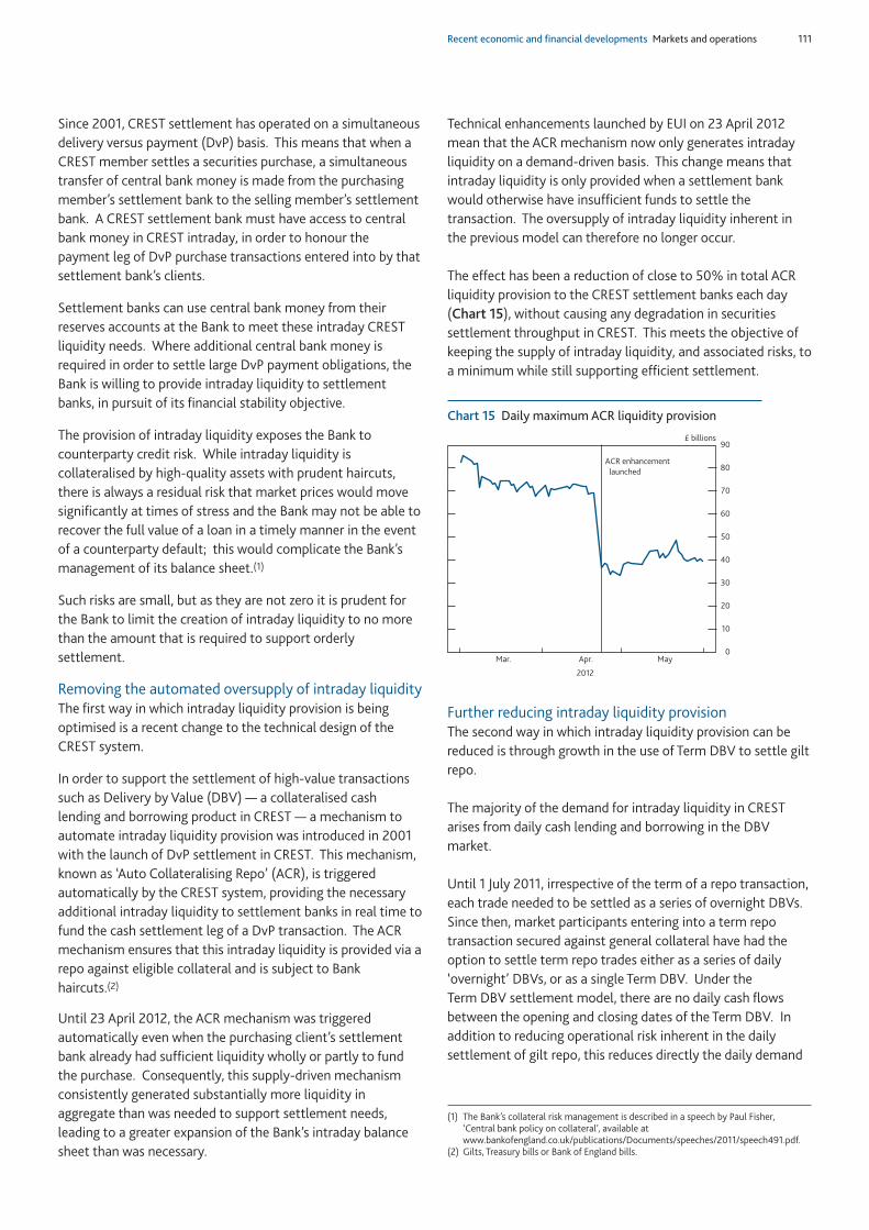
The effect has been a reduction of close to 50% in total ACRliquidity provision to the CREST settlement banks each day(Chart 15), without causing any degradation in securitiessettlement throughput in CREST. This meets the objective ofkeeping the supply of intraday liquidity, and associated risks, toa minimum while still supporting efficient settlement.
Further reducing intraday liquidity provisionThe second way in which intraday liquidity provision can bereduced is through growth in the use of Term DBV to settle giltrepo.
The majority of the demand for intraday liquidity in CRESTarises from daily cash lending and borrowing in the DBVmarket.
Until 1 July 2011, irrespective of the term of a repo transaction,each trade needed to be settled as a series of overnight DBVs.Since then, market participants entering into a term repotransaction secured against general collateral have had theoption to settle term repo trades either as a series of daily‘overnight’ DBVs, or as a single Term DBV. Under the Term DBV settlement model, there are no daily cash flowsbetween the opening and closing dates of the Term DBV. Inaddition to reducing operational risk inherent in the dailysettlement of gilt repo, this reduces directly the daily demand
(1) The Bank’s collateral risk management is described in a speech by Paul Fisher, ‘Central bank policy on collateral’, available atwww.bankofengland.co.uk/publications/Documents/speeches/2011/speech491.pdf.
(2) Gilts, Treasury bills or Bank of England bills.
0
10
20
30
40
50
60
70
80
90
Mar. Apr. May
£ billions
2012
ACR enhancement
launched
Chart 15 Daily maximum ACR liquidity provision

112 Quarterly Bulletin 2012 Q2
for intraday liquidity (supplied in practice by ACR), comparedwith the settlement of daily unwinds and re-inputs under theovernight DBV settlement model.(1)
At end-May 2012, approximately 4% of total DBV settlementvalue in CREST was Term DBV (the remainder being overnightDBV). This suggests that many genuinely term transactionsare still being settled as overnight DBVs. Market intelligencesuggests an impediment to greater use of Term DBV is that atpresent no central counterparty service provider can centrally
clear the transactions. LCH.Clearnet Ltd is working with itsclients and with EUI to schedule the development of a newcentrally cleared Term DBV product. It is expected that theuse of Term DBV could rise further when the new product isintroduced.
Given the risk-reduction benefits of widespread marketadoption of Term DBV, the Bank is supportive of furthergrowth in the use of this method of settlement and the stepsthat will facilitate this outcome.(2)
(1) The ‘Markets and operations’ article in the 2011 Q3 Quarterly Bulletin described theintroduction of the CREST ‘Term DBV’ service in July 2011 (pages 197–98).
(2) See the speech by Chris Salmon on 5 July 2011, ‘The case for more CHAPS settlementbanks’, available atwww.bankofengland.co.uk/publications/Documents/speeches/2011/speech508.pdf,and the Market Notice, available atwww.bankofengland.co.uk/markets/Documents/marketnotice110615.pdf.

Research and analysis
Quarterly Bulletin Research and analysis 113
114 Quarterly Bulletin 2012 Q2
Introduction
Inflation, as measured by the consumer prices index (CPI), hasbeen more than 1 percentage point above the 2% target set bythe Government for much of the past four years. That largelyreflects the temporary effects of a range of factors: rising foodand energy prices, changes in the standard rate of VAT andhigher import prices following the substantial depreciation insterling.
As inflation rose between 2010 and 2011 H1, the MonetaryPolicy Committee (MPC) became increasingly concerned thata continued period of above-target inflation might prompthouseholds, companies and financial market participants toexpect inflation to persist above the target. That mighthappen if individuals believed that the MPC had become more tolerant of deviations of inflation from target in the near term. Or if they had doubts about the ability, orwillingness, of the MPC to return inflation to target in themedium term. Either would suggest that expectations ofinflation had become less well anchored by the monetarypolicy framework. If inflation expectations were to becomeless well anchored, changes in price-setting or wage-settingbehaviour, or both, may lead inflation itself to become morepersistent. As a result, during 2011, the MPC judged there wasan upside risk to inflation from inflation expectations.
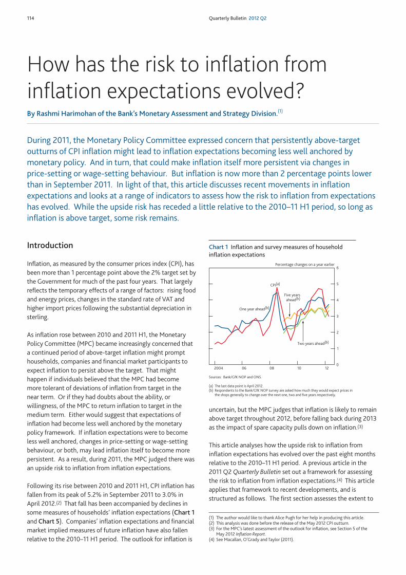
Following its rise between 2010 and 2011 H1, CPI inflation hasfallen from its peak of 5.2% in September 2011 to 3.0% inApril 2012.(2) That fall has been accompanied by declines insome measures of households’ inflation expectations (Chart 1and Chart 5). Companies’ inflation expectations and financialmarket implied measures of future inflation have also fallenrelative to the 2010–11 H1 period. The outlook for inflation is
uncertain, but the MPC judges that inflation is likely to remainabove target throughout 2012, before falling back during 2013as the impact of spare capacity pulls down on inflation.(3)
This article analyses how the upside risk to inflation frominflation expectations has evolved over the past eight monthsrelative to the 2010–11 H1 period. A previous article in the2011 Q2 Quarterly Bulletin set out a framework for assessingthe risk to inflation from inflation expectations.(4) This articleapplies that framework to recent developments, and isstructured as follows. The first section assesses the extent to
During 2011, the Monetary Policy Committee expressed concern that persistently above-targetoutturns of CPI inflation might lead to inflation expectations becoming less well anchored bymonetary policy. And in turn, that could make inflation itself more persistent via changes in price-setting or wage-setting behaviour. But inflation is now more than 2 percentage points lowerthan in September 2011. In light of that, this article discusses recent movements in inflationexpectations and looks at a range of indicators to assess how the risk to inflation from expectationshas evolved. While the upside risk has receded a little relative to the 2010–11 H1 period, so long asinflation is above target, some risk remains.
How has the risk to inflation frominflation expectations evolved?By Rashmi Harimohan of the Bank’s Monetary Assessment and Strategy Division.(1)
(1) The author would like to thank Alice Pugh for her help in producing this article. (2) This analysis was done before the release of the May 2012 CPI outturn. (3) For the MPC’s latest assessment of the outlook for inflation, see Section 5 of the
May 2012 Inflation Report.(4) See Macallan, O’Grady and Taylor (2011).
0
1
2
3
4
5
6
2004 06 08 10 12
One year ahead(b)
Two years ahead(b)
Five years
ahead(b)
CPI(a)
Percentage changes on a year earlier
Chart 1 Inflation and survey measures of householdinflation expectations
Sources: Bank/GfK NOP and ONS.
(a) The last data point is April 2012.(b) Respondents to the Bank/GfK NOP survey are asked how much they would expect prices in
the shops generally to change over the next one, two and five years respectively.
Research and analysis Risk to inflation from inflation expectations 115
which long-term and short-term expectations remain wellanchored. The second section evaluates the latest evidence onthe extent to which inflation expectations have affected wageand price-setting behaviour. The final section concludes.
Assessing the extent to which expectationsremain anchored
Inflation expectations could become less well anchored in twoways. First, households, companies and financial marketparticipants may become less confident in the ability, orwillingness, of the MPC to bring inflation back to target in themedium to long term. Second, they may perceive the MPC tohave become more tolerant of deviations in inflation fromtarget in the near term, and, therefore, expect inflation toreturn towards the target more slowly. The former would besignalled by changes in longer-term expectations, and thelatter would be reflected in shorter-term measures. Thissection therefore reviews movements in both longer-term andshorter-term expectations over the past eight months toassess how the upside risk to inflation from inflationexpectations has evolved relative to 2010–11 H1.
Longer-term expectationsIf inflation expectations were to become less well anchored tothe inflation target in the longer term, then this might becomeevident in at least one of three ways: the level of inflationexpectations might deviate from target; inflation expectationsmight become more responsive to developments in the
economy; and uncertainty around expected future inflationmight increase.
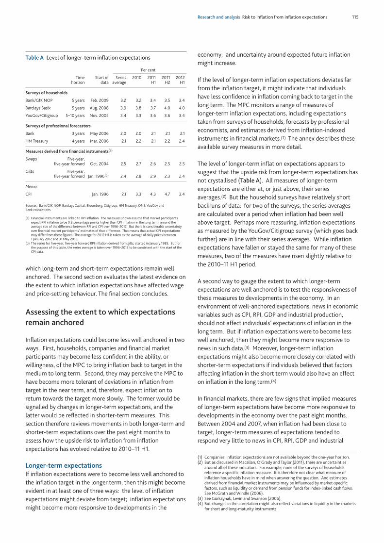
If the level of longer-term inflation expectations deviates farfrom the inflation target, it might indicate that individualshave less confidence in inflation coming back to target in thelong term. The MPC monitors a range of measures of longer-term inflation expectations, including expectationstaken from surveys of households, forecasts by professionaleconomists, and estimates derived from inflation-indexedinstruments in financial markets.(1) The annex describes theseavailable survey measures in more detail.
The level of longer-term inflation expectations appears tosuggest that the upside risk from longer-term expectations hasnot crystallised (Table A). All measures of longer-termexpectations are either at, or just above, their seriesaverages.(2) But the household surveys have relatively shortbackruns of data: for two of the surveys, the series averagesare calculated over a period when inflation had been wellabove target. Perhaps more reassuring, inflation expectationsas measured by the YouGov/Citigroup survey (which goes backfurther) are in line with their series averages. While inflationexpectations have fallen or stayed the same for many of thesemeasures, two of the measures have risen slightly relative tothe 2010–11 H1 period.
A second way to gauge the extent to which longer-termexpectations are well anchored is to test the responsiveness ofthese measures to developments in the economy. In anenvironment of well-anchored expectations, news in economicvariables such as CPI, RPI, GDP and industrial production,should not affect individuals’ expectations of inflation in thelong term. But if inflation expectations were to become lesswell anchored, then they might become more responsive tonews in such data.(3) Moreover, longer-term inflationexpectations might also become more closely correlated withshorter-term expectations if individuals believed that factorsaffecting inflation in the short term would also have an effecton inflation in the long term.(4)
In financial markets, there are few signs that implied measuresof longer-term expectations have become more responsive todevelopments in the economy over the past eight months.Between 2004 and 2007, when inflation had been close totarget, longer-term measures of expectations tended torespond very little to news in CPI, RPI, GDP and industrial
Table A Level of longer-term inflation expectations
Per cent
Time Start of Series 2010 2011 2011 2012horizon data average H1 H2 H1
Surveys of households
Bank/GfK NOP 5 years Feb. 2009 3.2 3.2 3.4 3.5 3.4
Barclays Basix 5 years Aug. 2008 3.9 3.8 3.7 4.0 4.0
YouGov/Citigroup 5–10 years Nov. 2005 3.4 3.3 3.6 3.6 3.4
Surveys of professional forecasters
Bank 3 years May 2006 2.0 2.0 2.1 2.1 2.1
HM Treasury 4 years Mar. 2006 2.1 2.2 2.1 2.2 2.4
Measures derived from financial instruments(a)
Swaps Five-year, five-year forward Oct. 2004 2.5 2.7 2.6 2.5 2.5
Gilts Five-year,five-year forward Jan. 1996(b) 2.4 2.8 2.9 2.3 2.4
Memo:
CPI Jan. 1996 2.1 3.3 4.3 4.7 3.4
Sources: Bank/GfK NOP, Barclays Capital, Bloomberg, Citigroup, HM Treasury, ONS, YouGov and Bank calculations.
(a) Financial instruments are linked to RPI inflation. The measures shown assume that market participantsexpect RPI inflation to be 0.8 percentage points higher than CPI inflation in the long term, around theaverage size of the difference between RPI and CPI over 1996–2012. But there is considerable uncertaintyover financial market participants’ estimates of that difference. That means that actual CPI expectationsmay differ from these figures. The average for 2012 H1 is taken as the average of daily prices between1 January 2012 and 31 May 2012.
(b) The series for five-year, five-year forward RPI inflation derived from gilts, started in January 1985. But for the purpose of this table, the series average is taken over 1996–2012 to be consistent with the start of theCPI data.
(1) Companies’ inflation expectations are not available beyond the one-year horizon.(2) But as discussed in Macallan, O’Grady and Taylor (2011), there are uncertainties
around all of these indicators. For example, none of the surveys of householdsreference a specific inflation measure. It is therefore not clear what measure ofinflation households have in mind when answering the question. And estimatesderived from financial market instruments may be influenced by market-specificfactors, such as liquidity or demand from pension funds for index-linked cash flows.See McGrath and Windle (2006).
(3) See Gürkaynak, Levin and Swanson (2006).(4) But changes in the correlation might also reflect variations in liquidity in the markets
for short and long-maturity instruments.
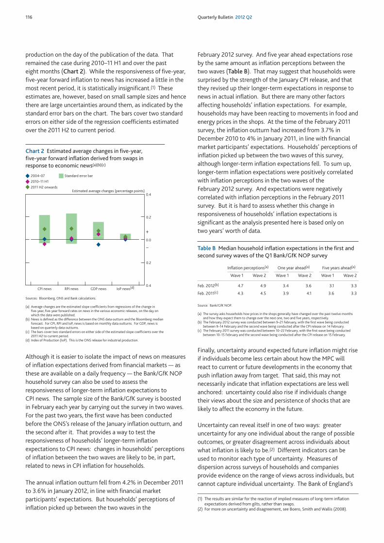
116 Quarterly Bulletin 2012 Q2
production on the day of the publication of the data. Thatremained the case during 2010–11 H1 and over the pasteight months (Chart 2). While the responsiveness of five-year,five-year forward inflation to news has increased a little in themost recent period, it is statistically insignificant.(1) Theseestimates are, however, based on small sample sizes and hencethere are large uncertainties around them, as indicated by thestandard error bars on the chart. The bars cover two standarderrors on either side of the regression coefficients estimatedover the 2011 H2 to current period.
Although it is easier to isolate the impact of news on measuresof inflation expectations derived from financial markets — asthese are available on a daily frequency — the Bank/GfK NOPhousehold survey can also be used to assess theresponsiveness of longer-term inflation expectations toCPI news. The sample size of the Bank/GfK survey is boostedin February each year by carrying out the survey in two waves.For the past two years, the first wave has been conductedbefore the ONS’s release of the January inflation outturn, andthe second after it. That provides a way to test theresponsiveness of households’ longer-term inflationexpectations to CPI news: changes in households’ perceptionsof inflation between the two waves are likely to be, in part,related to news in CPI inflation for households.
The annual inflation outturn fell from 4.2% in December 2011to 3.6% in January 2012, in line with financial marketparticipants’ expectations. But households’ perceptions ofinflation picked up between the two waves in the
February 2012 survey. And five year ahead expectations roseby the same amount as inflation perceptions between the two waves (Table B). That may suggest that households weresurprised by the strength of the January CPI release, and thatthey revised up their longer-term expectations in response tonews in actual inflation. But there are many other factorsaffecting households’ inflation expectations. For example,households may have been reacting to movements in food andenergy prices in the shops. At the time of the February 2011survey, the inflation outturn had increased from 3.7% inDecember 2010 to 4% in January 2011, in line with financialmarket participants’ expectations. Households’ perceptions ofinflation picked up between the two waves of this survey,although longer-term inflation expectations fell. To sum up,longer-term inflation expectations were positively correlatedwith inflation perceptions in the two waves of theFebruary 2012 survey. And expectations were negativelycorrelated with inflation perceptions in the February 2011survey. But it is hard to assess whether this change inresponsiveness of households’ inflation expectations issignificant as the analysis presented here is based only on two years’ worth of data.
Finally, uncertainty around expected future inflation might riseif individuals become less certain about how the MPC willreact to current or future developments in the economy thatpush inflation away from target. That said, this may notnecessarily indicate that inflation expectations are less wellanchored: uncertainty could also rise if individuals changetheir views about the size and persistence of shocks that arelikely to affect the economy in the future.
Uncertainty can reveal itself in one of two ways: greateruncertainty for any one individual about the range of possibleoutcomes, or greater disagreement across individuals aboutwhat inflation is likely to be.(2) Different indicators can beused to monitor each type of uncertainty. Measures ofdispersion across surveys of households and companiesprovide evidence on the range of views across individuals, butcannot capture individual uncertainty. The Bank of England’s
(1) The results are similar for the reaction of implied measures of long-term inflationexpectations derived from gilts, rather than swaps.
(2) For more on uncertainty and disagreement, see Boero, Smith and Wallis (2008).
0.4
0.2
0.0
0.2
0.4
CPI news RPI news GDP news IoP news(d)
2004–07
2010–11 H1
2011 H2 onwardsEstimated average changes (percentage points)
+
–
Standard error bar
Chart 2 Estimated average changes in five-year, five-year forward inflation derived from swaps inresponse to economic news(a)(b)(c)
Sources: Bloomberg, ONS and Bank calculations.
(a) Average changes are the estimated slope coefficients from regressions of the change in five-year, five-year forward rates on news in the various economic releases, on the day onwhich the data were published.
(b) News is defined as the difference between the ONS data outturn and the Bloomberg medianforecast. For CPI, RPI and IoP, news is based on monthly data outturns. For GDP, news isbased on quarterly data outturns.
(c) The bars cover two standard errors on either side of the estimated slope coefficients over the2011 H2 to current period.
(d) Index of Production (IoP). This is the ONS release for industrial production.
Table B Median household inflation expectations in the first andsecond survey waves of the Q1 Bank/GfK NOP survey
Inflation perceptions(a) One year ahead(a) Five years ahead(a)
Wave 1 Wave 2 Wave 1 Wave 2 Wave 1 Wave 2
Feb. 2012(b) 4.7 4.9 3.4 3.6 3.1 3.3
Feb. 2011(c) 4.3 4.5 3.9 4.1 3.6 3.3
Source: Bank/GfK NOP.
(a) The survey asks households how prices in the shops generally have changed over the past twelve monthsand how they expect them to change over the next one, two and five years, respectively.
(b) The February 2012 survey was conducted between 9–21 February, with the first wave being conductedbetween 9–14 February and the second wave being conducted after the CPI release on 14 February.
(c) The February 2011 survey was conducted between 10–22 February, with the first wave being conductedbetween 10–15 February and the second wave being conducted after the CPI release on 15 February.
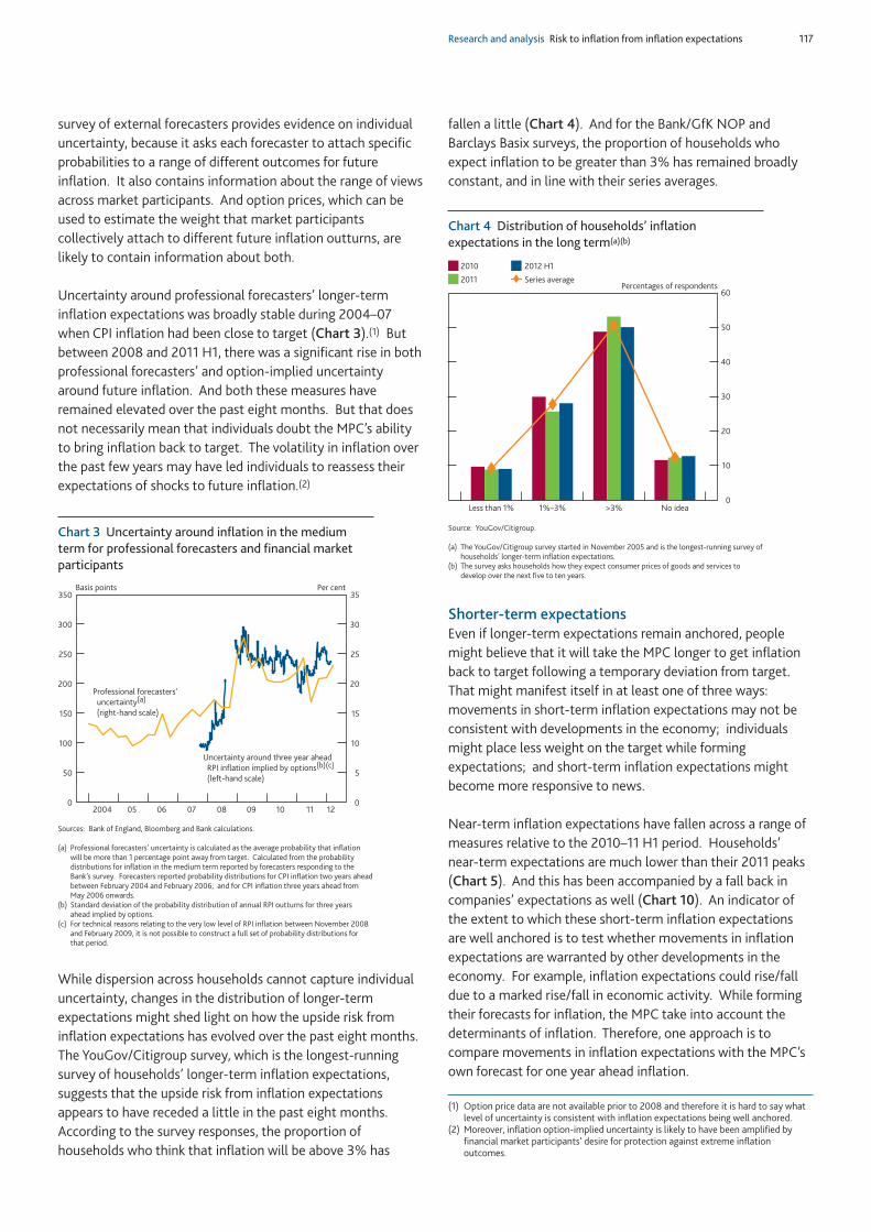
Research and analysis Risk to inflation from inflation expectations 117
survey of external forecasters provides evidence on individualuncertainty, because it asks each forecaster to attach specificprobabilities to a range of different outcomes for futureinflation. It also contains information about the range of viewsacross market participants. And option prices, which can beused to estimate the weight that market participantscollectively attach to different future inflation outturns, arelikely to contain information about both.
Uncertainty around professional forecasters’ longer-terminflation expectations was broadly stable during 2004–07when CPI inflation had been close to target (Chart 3).(1) Butbetween 2008 and 2011 H1, there was a significant rise in bothprofessional forecasters’ and option-implied uncertaintyaround future inflation. And both these measures haveremained elevated over the past eight months. But that doesnot necessarily mean that individuals doubt the MPC’s abilityto bring inflation back to target. The volatility in inflation overthe past few years may have led individuals to reassess theirexpectations of shocks to future inflation.(2)
While dispersion across households cannot capture individualuncertainty, changes in the distribution of longer-termexpectations might shed light on how the upside risk frominflation expectations has evolved over the past eight months.The YouGov/Citigroup survey, which is the longest-runningsurvey of households’ longer-term inflation expectations,suggests that the upside risk from inflation expectationsappears to have receded a little in the past eight months.According to the survey responses, the proportion ofhouseholds who think that inflation will be above 3% has
fallen a little (Chart 4). And for the Bank/GfK NOP andBarclays Basix surveys, the proportion of households whoexpect inflation to be greater than 3% has remained broadlyconstant, and in line with their series averages.
Shorter-term expectationsEven if longer-term expectations remain anchored, peoplemight believe that it will take the MPC longer to get inflationback to target following a temporary deviation from target.That might manifest itself in at least one of three ways:movements in short-term inflation expectations may not beconsistent with developments in the economy; individualsmight place less weight on the target while formingexpectations; and short-term inflation expectations mightbecome more responsive to news.
Near-term inflation expectations have fallen across a range ofmeasures relative to the 2010–11 H1 period. Households’near-term expectations are much lower than their 2011 peaks(Chart 5). And this has been accompanied by a fall back incompanies’ expectations as well (Chart 10). An indicator ofthe extent to which these short-term inflation expectationsare well anchored is to test whether movements in inflationexpectations are warranted by other developments in theeconomy. For example, inflation expectations could rise/falldue to a marked rise/fall in economic activity. While formingtheir forecasts for inflation, the MPC take into account thedeterminants of inflation. Therefore, one approach is tocompare movements in inflation expectations with the MPC’sown forecast for one year ahead inflation.
0
50
100
150
200
250
300
350
0
10
20
30
2004 05 06 07 08 09 10 11 12
Per cent Basis points
Professional forecasters’
uncertainty(a)
(right-hand scale)
Uncertainty around three year ahead
RPI inflation implied by options(b)(c)
(left-hand scale)
35
25
15
5
Chart 3 Uncertainty around inflation in the mediumterm for professional forecasters and financial marketparticipants
Sources: Bank of England, Bloomberg and Bank calculations.
(a) Professional forecasters’ uncertainty is calculated as the average probability that inflationwill be more than 1 percentage point away from target. Calculated from the probabilitydistributions for inflation in the medium term reported by forecasters responding to theBank’s survey. Forecasters reported probability distributions for CPI inflation two years aheadbetween February 2004 and February 2006; and for CPI inflation three years ahead fromMay 2006 onwards.
(b) Standard deviation of the probability distribution of annual RPI outturns for three yearsahead implied by options.
(c) For technical reasons relating to the very low level of RPI inflation between November 2008and February 2009, it is not possible to construct a full set of probability distributions forthat period.
0
10
20
30
40
50
60
Less than 1% 1%–3% >3% No idea
2010
2011
2012 H1
Series averagePercentages of respondents
Chart 4 Distribution of households’ inflationexpectations in the long term(a)(b)
Source: YouGov/Citigroup.
(a) The YouGov/Citigroup survey started in November 2005 and is the longest-running survey ofhouseholds’ longer-term inflation expectations.
(b) The survey asks households how they expect consumer prices of goods and services todevelop over the next five to ten years.
(1) Option price data are not available prior to 2008 and therefore it is hard to say whatlevel of uncertainty is consistent with inflation expectations being well anchored.
(2) Moreover, inflation option-implied uncertainty is likely to have been amplified byfinancial market participants’ desire for protection against extreme inflationoutcomes.
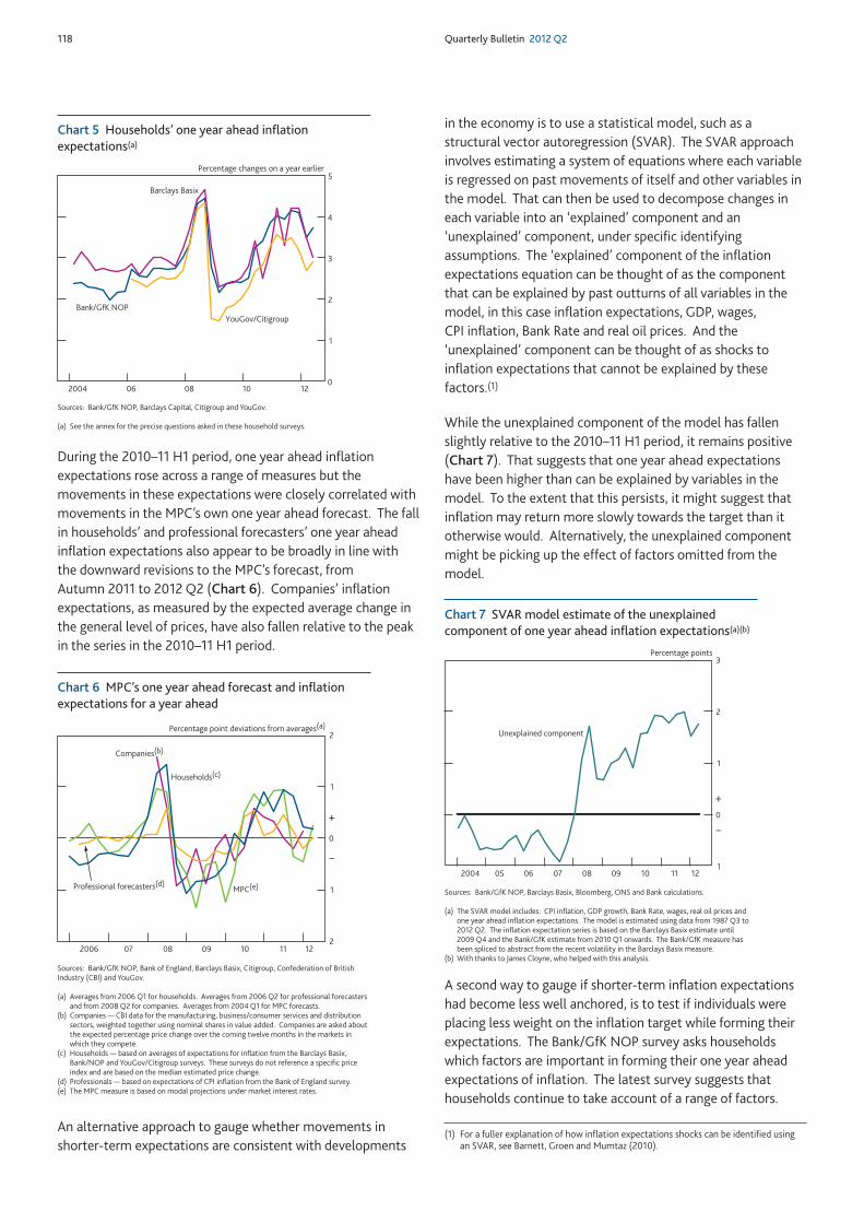
118 Quarterly Bulletin 2012 Q2
During the 2010–11 H1 period, one year ahead inflationexpectations rose across a range of measures but themovements in these expectations were closely correlated withmovements in the MPC’s own one year ahead forecast. The fallin households’ and professional forecasters’ one year aheadinflation expectations also appear to be broadly in line withthe downward revisions to the MPC’s forecast, fromAutumn 2011 to 2012 Q2 (Chart 6). Companies’ inflationexpectations, as measured by the expected average change inthe general level of prices, have also fallen relative to the peakin the series in the 2010–11 H1 period.
An alternative approach to gauge whether movements inshorter-term expectations are consistent with developments
in the economy is to use a statistical model, such as astructural vector autoregression (SVAR). The SVAR approachinvolves estimating a system of equations where each variableis regressed on past movements of itself and other variables inthe model. That can then be used to decompose changes ineach variable into an ‘explained’ component and an‘unexplained’ component, under specific identifyingassumptions. The ‘explained’ component of the inflationexpectations equation can be thought of as the componentthat can be explained by past outturns of all variables in themodel, in this case inflation expectations, GDP, wages,CPI inflation, Bank Rate and real oil prices. And the‘unexplained’ component can be thought of as shocks toinflation expectations that cannot be explained by thesefactors.(1)
While the unexplained component of the model has fallenslightly relative to the 2010–11 H1 period, it remains positive(Chart 7). That suggests that one year ahead expectationshave been higher than can be explained by variables in themodel. To the extent that this persists, it might suggest thatinflation may return more slowly towards the target than itotherwise would. Alternatively, the unexplained componentmight be picking up the effect of factors omitted from themodel.
A second way to gauge if shorter-term inflation expectationshad become less well anchored, is to test if individuals wereplacing less weight on the inflation target while forming theirexpectations. The Bank/GfK NOP survey asks householdswhich factors are important in forming their one year aheadexpectations of inflation. The latest survey suggests thathouseholds continue to take account of a range of factors.
2
1
0
1
2
2006 07 08 09 10 11 12
Percentage point deviations from averages(a)
Companies(b)
Professional forecasters(d)MPC(e)
Households(c)
+
–
Chart 6 MPC’s one year ahead forecast and inflationexpectations for a year ahead
Sources: Bank/GfK NOP, Bank of England, Barclays Basix, Citigroup, Confederation of BritishIndustry (CBI) and YouGov.
(a) Averages from 2006 Q1 for households. Averages from 2006 Q2 for professional forecastersand from 2008 Q2 for companies. Averages from 2004 Q1 for MPC forecasts.
(b) Companies — CBI data for the manufacturing, business/consumer services and distributionsectors, weighted together using nominal shares in value added. Companies are asked aboutthe expected percentage price change over the coming twelve months in the markets inwhich they compete.
(c) Households — based on averages of expectations for inflation from the Barclays Basix,Bank/NOP and YouGov/Citigroup surveys. These surveys do not reference a specific priceindex and are based on the median estimated price change.
(d) Professionals — based on expectations of CPI inflation from the Bank of England survey.(e) The MPC measure is based on modal projections under market interest rates.
1
0
1
2
3
2004 05 06 07 08 09 10 11 12
Unexplained component
Percentage points
+
–
Chart 7 SVAR model estimate of the unexplainedcomponent of one year ahead inflation expectations(a)(b)
Sources: Bank/GfK NOP, Barclays Basix, Bloomberg, ONS and Bank calculations.
(a) The SVAR model includes: CPI inflation, GDP growth, Bank Rate, wages, real oil prices andone year ahead inflation expectations. The model is estimated using data from 1987 Q3 to2012 Q2. The inflation expectation series is based on the Barclays Basix estimate until2009 Q4 and the Bank/GfK estimate from 2010 Q1 onwards. The Bank/GfK measure hasbeen spliced to abstract from the recent volatility in the Barclays Basix measure.
(b) With thanks to James Cloyne, who helped with this analysis.
(1) For a fuller explanation of how inflation expectations shocks can be identified usingan SVAR, see Barnett, Groen and Mumtaz (2010).
0
1
2
3
4
5
2004 06 08 10 12
Bank/GfK NOP
Barclays Basix
YouGov/Citigroup
Percentage changes on a year earlier
Chart 5 Households’ one year ahead inflationexpectations(a)
Sources: Bank/GfK NOP, Barclays Capital, Citigroup and YouGov.
(a) See the annex for the precise questions asked in these household surveys.
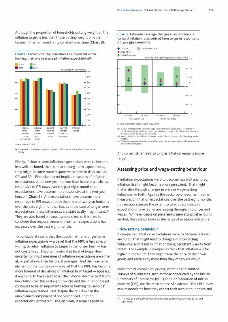
Research and analysis Risk to inflation from inflation expectations 119
Although the proportion of households putting weight on theinflation target is less than those putting weight on otherfactors, it has remained fairly constant over time (Chart 8).
Finally, if shorter-term inflation expectations were to becomeless well anchored, then, similar to long-term expectations,they might become more responsive to news in data such asCPI and RPI. Financial market implied measures of inflationexpectations at the one-year horizon have become a little lessresponsive to CPI news over the past eight months butexpectations have become more responsive at the two-yearhorizon (Chart 9). And expectations have become moreresponsive to RPI news at both the one and two-year horizonsover the past eight months. But, as in the case of longer-termexpectations, these differences are statistically insignificant.(1)
They are also based on small sample sizes, so it is hard toconclude that responsiveness of near-term expectations hasincreased over the past eight months.
To conclude, it seems that the upside risk from longer-terminflation expectations — a belief that the MPC is less able, orwilling, to return inflation to target in the longer term — hasnot crystallised. Despite the elevated level of longer-termuncertainty, most measures of inflation expectations are eitherat, or just above, their historical averages. And the near-termelement of the upside risk — a belief that the MPC has becomemore tolerant of deviations of inflation from target — appears,if anything, to have receded a little. Shorter-term expectationshave fallen over the past eight months and the inflation targetcontinues to be an important factor in forming households’inflation expectations. But despite the tick down in theunexplained component of one year ahead inflationexpectations, estimated using an SVAR, it remains positive.
And some risk remains so long as inflation remains abovetarget.
Assessing price and wage-setting behaviour
If inflation expectations were to become less well anchored,inflation itself might become more persistent. That mightmaterialise through changes in price or wage-settingbehaviour, or both. Against the backdrop of declines in somemeasures of inflation expectations over the past eight months,this section assesses the extent to which past inflationexpectations have fed, or are feeding through, into prices andwages. While evidence on price and wage-setting behaviour islimited, this section looks at the range of available indicators.
Price-setting behaviourIf companies’ inflation expectations were to become less wellanchored, that might lead to changes in price-settingbehaviour, and result in inflation being persistently away fromtarget. For example, if companies think that inflation will behigher in the future, they might raise the price of their owngoods and services by more than they otherwise would.
Indicators of companies’ pricing intentions are limited.Surveys of businesses, such as those conducted by the BritishChambers of Commerce (BCC) and Confederation of BritishIndustry (CBI), are the main source of evidence. The CBI surveyasks respondents how they expect their own output prices and
0
10
20
30
40
50
60
70
80
90
100
2009
2010
2011
2012Percentages of respondents
Inflation
in the
previous
one to
six months
Inflation
in the
previous
year or
before
Current
level of
interest
rates
Current
strength
of the UK
economy
Inflation
target
Chart 8 Factors cited by households as important whenforming their one year ahead inflation expectations(a)
Source: Bank/GfK NOP.
(a) Respondents could select more than one option. The question is only asked in the extendedsurvey.
0.4
0.0
0.4
CPI news RPI news CPI news RPI news
Estimated average changes (percentage points)
One year ahead Two years ahead
2004–07
2010–11 H1
2011 H2 onwards
+
–
0.2
0.6
0.2
0.6
Standard error bar
Chart 9 Estimated average changes in instantaneousforward inflation rates derived from swaps in response toCPI and RPI news(a)(b)(c)
Sources: Bloomberg, ONS and Bank calculations.
(a) Average changes are the estimated slope coefficients from regressions of the change ininstantaneous forward inflation rates at each horizon on news in the CPI and RPI releases, onthe day on which the data were published.
(b) News is defined as the difference between the ONS data outturn and the Bloomberg medianforecast.
(c) The bars cover two standard errors on either side of the estimated slope coefficients over the2011 H2 to current period.
(1) The results are broadly similar when looking at the responsiveness to IoP and GDP news.
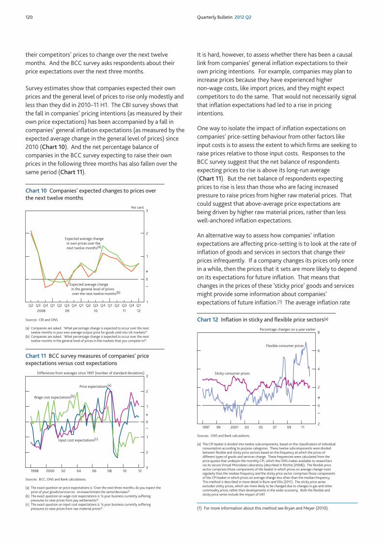
120 Quarterly Bulletin 2012 Q2
their competitors’ prices to change over the next twelvemonths. And the BCC survey asks respondents about theirprice expectations over the next three months.
Survey estimates show that companies expected their ownprices and the general level of prices to rise only modestly andless than they did in 2010–11 H1. The CBI survey shows thatthe fall in companies’ pricing intentions (as measured by theirown price expectations) has been accompanied by a fall incompanies’ general inflation expectations (as measured by theexpected average change in the general level of prices) since2010 (Chart 10). And the net percentage balance ofcompanies in the BCC survey expecting to raise their ownprices in the following three months has also fallen over thesame period (Chart 11).
It is hard, however, to assess whether there has been a causallink from companies’ general inflation expectations to theirown pricing intentions. For example, companies may plan toincrease prices because they have experienced higher non-wage costs, like import prices, and they might expectcompetitors to do the same. That would not necessarily signalthat inflation expectations had led to a rise in pricingintentions.
One way to isolate the impact of inflation expectations oncompanies’ price-setting behaviour from other factors likeinput costs is to assess the extent to which firms are seeking toraise prices relative to those input costs. Responses to the BCC survey suggest that the net balance of respondentsexpecting prices to rise is above its long-run average(Chart 11). But the net balance of respondents expectingprices to rise is less than those who are facing increasedpressure to raise prices from higher raw material prices. Thatcould suggest that above-average price expectations are being driven by higher raw material prices, rather than less well-anchored inflation expectations.
An alternative way to assess how companies’ inflationexpectations are affecting price-setting is to look at the rate ofinflation of goods and services in sectors that change theirprices infrequently. If a company changes its prices only oncein a while, then the prices that it sets are more likely to dependon its expectations for future inflation. That means thatchanges in the prices of these ‘sticky price’ goods and servicesmight provide some information about companies’expectations of future inflation.(1) The average inflation rate
3
2
1
0
1
2
3
1998 2000 02 04 06 08 10 12
Price expectations(a)
Input cost expectations(c)
Wage cost expectations(b)
Differences from averages since 1997 (number of standard deviations)
+
–
Chart 11 BCC survey measures of companies’ priceexpectations versus cost expectations
Sources: BCC, ONS and Bank calculations.
(a) The exact question on price expectations is ‘Over the next three months, do you expect theprice of your goods/services to: increase/remain the same/decrease?’.
(b) The exact question on wage cost expectations is ‘Is your business currently sufferingpressures to raise prices from pay settlements?’.
(c) The exact question on input cost expectations is ‘Is your business currently sufferingpressures to raise prices from raw material prices?’.
1
0
1
2
3
Q2
2008
Q2
09
Q2
10
Q2
11
Per cent
Expected average change
in own prices over the
next twelve months(a)
Expected average change
in the general level of prices
over the next twelve months(b)
+
–
Q4 Q4 Q4 Q4
12
Q3 Q3 Q3 Q3Q1 Q1 Q1 Q1
Chart 10 Companies’ expected changes to prices overthe next twelve months
Sources: CBI and ONS.
(a) Companies are asked: ‘What percentage change is expected to occur over the nexttwelve months in your own average output price for goods sold into UK markets?’.
(b) Companies are asked: ‘What percentage change is expected to occur over the nexttwelve months in the general level of prices in the markets that you compete in?’.
(1) For more information about this method see Bryan and Meyer (2010).
2
0
2
4
6
8
1997 99 2001 03 05 07 09 11
Percentage changes on a year earlier
Sticky consumer prices
Flexible consumer prices
+
–
Chart 12 Inflation in sticky and flexible price sectors(a)
Sources: ONS and Bank calculations.
(a) The CPI basket is divided into twelve subcomponents, based on the classification of individualconsumption according to purpose categories. These twelve subcomponents were dividedbetween flexible and sticky price sectors based on the frequency at which the prices ofdifferent types of goods and services change. These frequencies were calculated from theprice quotes that underpin the monthly CPI, which the ONS makes available to researchersvia its secure Virtual Microdata Laboratory (described in Ritchie (2008)). The flexible pricesector comprises those components of the basket in which prices on average change moreregularly than the median frequency and the sticky price sector comprises those componentsof the CPI basket in which prices on average change less often than the median frequency.This method is described in more detail in Bunn and Ellis (2011). The sticky price seriesexcludes utility prices, which are more likely to be changed due to changes in gas and othercommodity prices rather than developments in the wider economy. Both the flexible andsticky price series include the impact of VAT.
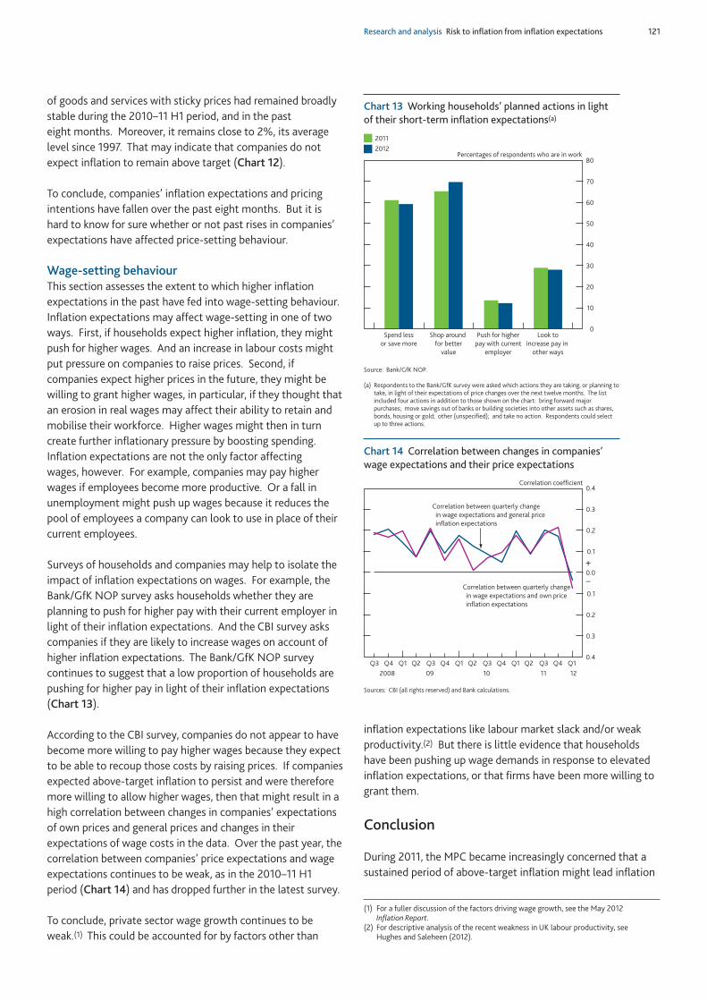
Research and analysis Risk to inflation from inflation expectations 121
of goods and services with sticky prices had remained broadlystable during the 2010–11 H1 period, and in the past eight months. Moreover, it remains close to 2%, its averagelevel since 1997. That may indicate that companies do notexpect inflation to remain above target (Chart 12).
To conclude, companies’ inflation expectations and pricingintentions have fallen over the past eight months. But it ishard to know for sure whether or not past rises in companies’expectations have affected price-setting behaviour.
Wage-setting behaviourThis section assesses the extent to which higher inflationexpectations in the past have fed into wage-setting behaviour.Inflation expectations may affect wage-setting in one of twoways. First, if households expect higher inflation, they mightpush for higher wages. And an increase in labour costs mightput pressure on companies to raise prices. Second, ifcompanies expect higher prices in the future, they might bewilling to grant higher wages, in particular, if they thought thatan erosion in real wages may affect their ability to retain andmobilise their workforce. Higher wages might then in turncreate further inflationary pressure by boosting spending.Inflation expectations are not the only factor affecting wages, however. For example, companies may pay higherwages if employees become more productive. Or a fall inunemployment might push up wages because it reduces thepool of employees a company can look to use in place of theircurrent employees.
Surveys of households and companies may help to isolate theimpact of inflation expectations on wages. For example, theBank/GfK NOP survey asks households whether they areplanning to push for higher pay with their current employer inlight of their inflation expectations. And the CBI survey askscompanies if they are likely to increase wages on account ofhigher inflation expectations. The Bank/GfK NOP surveycontinues to suggest that a low proportion of households arepushing for higher pay in light of their inflation expectations(Chart 13).
According to the CBI survey, companies do not appear to havebecome more willing to pay higher wages because they expectto be able to recoup those costs by raising prices. If companiesexpected above-target inflation to persist and were thereforemore willing to allow higher wages, then that might result in ahigh correlation between changes in companies’ expectationsof own prices and general prices and changes in theirexpectations of wage costs in the data. Over the past year, thecorrelation between companies’ price expectations and wageexpectations continues to be weak, as in the 2010–11 H1period (Chart 14) and has dropped further in the latest survey.
To conclude, private sector wage growth continues to beweak.(1) This could be accounted for by factors other than
inflation expectations like labour market slack and/or weakproductivity.(2) But there is little evidence that householdshave been pushing up wage demands in response to elevatedinflation expectations, or that firms have been more willing togrant them.
Conclusion
During 2011, the MPC became increasingly concerned that asustained period of above-target inflation might lead inflation
(1) For a fuller discussion of the factors driving wage growth, see the May 2012 Inflation Report.
(2) For descriptive analysis of the recent weakness in UK labour productivity, see Hughes and Saleheen (2012).
0.4
0.3
0.2
0.1
0.0
0.1
0.2
0.3
0.4
Correlation between quarterly change
in wage expectations and general price
inflation expectations
Correlation between quarterly change
in wage expectations and own price
inflation expectations
Correlation coefficient
Q2 Q2 Q2 Q4 Q4 Q4 Q4Q3 Q3 Q3 Q3Q1 Q1 Q1 Q1
2008 09 10 11 12
+
–
Chart 14 Correlation between changes in companies’wage expectations and their price expectations
Sources: CBI (all rights reserved) and Bank calculations.
0
10
20
30
40
50
60
70
80Percentages of respondents who are in work
2011
2012
Spend less
or save more
Shop around
for better
value
Push for higher
pay with current
employer
Look to
increase pay in
other ways
Chart 13 Working households’ planned actions in lightof their short-term inflation expectations(a)
Source: Bank/GfK NOP.
(a) Respondents to the Bank/GfK survey were asked which actions they are taking, or planning totake, in light of their expectations of price changes over the next twelve months. The listincluded four actions in addition to those shown on the chart: bring forward majorpurchases; move savings out of banks or building societies into other assets such as shares,bonds, housing or gold; other (unspecified); and take no action. Respondents could selectup to three actions.
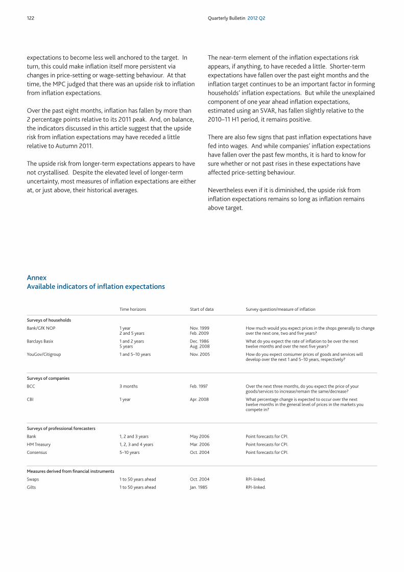
122 Quarterly Bulletin 2012 Q2
AnnexAvailable indicators of inflation expectations
Time horizons Start of data Survey question/measure of inflation
Surveys of households
Bank/GfK NOP 1 year Nov. 1999 How much would you expect prices in the shops generally to change 2 and 5 years Feb. 2009 over the next one, two and five years?
Barclays Basix 1 and 2 years Dec. 1986 What do you expect the rate of inflation to be over the next 5 years Aug. 2008 twelve months and over the next five years?
YouGov/Citigroup 1 and 5–10 years Nov. 2005 How do you expect consumer prices of goods and services will develop over the next 1 and 5–10 years, respectively?
Surveys of companies
BCC 3 months Feb. 1997 Over the next three months, do you expect the price of your goods/services to increase/remain the same/decrease?
CBI 1 year Apr. 2008 What percentage change is expected to occur over the next twelve months in the general level of prices in the markets youcompete in?
Surveys of professional forecasters
Bank 1, 2 and 3 years May 2006 Point forecasts for CPI.
HM Treasury 1, 2, 3 and 4 years Mar. 2006 Point forecasts for CPI.
Consensus 5–10 years Oct. 2004 Point forecasts for CPI.
Measures derived from financial instruments
Swaps 1 to 50 years ahead Oct. 2004 RPI-linked.
Gilts 1 to 50 years ahead Jan. 1985 RPI-linked.
expectations to become less well anchored to the target. Inturn, this could make inflation itself more persistent viachanges in price-setting or wage-setting behaviour. At thattime, the MPC judged that there was an upside risk to inflationfrom inflation expectations.
Over the past eight months, inflation has fallen by more than2 percentage points relative to its 2011 peak. And, on balance,the indicators discussed in this article suggest that the upsiderisk from inflation expectations may have receded a littlerelative to Autumn 2011.
The upside risk from longer-term expectations appears to havenot crystallised. Despite the elevated level of longer-termuncertainty, most measures of inflation expectations are eitherat, or just above, their historical averages.
The near-term element of the inflation expectations riskappears, if anything, to have receded a little. Shorter-termexpectations have fallen over the past eight months and theinflation target continues to be an important factor in forminghouseholds’ inflation expectations. But while the unexplainedcomponent of one year ahead inflation expectations,estimated using an SVAR, has fallen slightly relative to the2010–11 H1 period, it remains positive.
There are also few signs that past inflation expectations havefed into wages. And while companies’ inflation expectationshave fallen over the past few months, it is hard to know forsure whether or not past rises in these expectations haveaffected price-setting behaviour.
Nevertheless even if it is diminished, the upside risk frominflation expectations remains so long as inflation remainsabove target.

Research and analysis Risk to inflation from inflation expectations 123
References
Barnett, A, Groen, J and Mumtaz, H (2010), ‘Time-varying inflationexpectations and economic fluctuations in the United Kingdom: astructural VAR analysis’, Bank of England Working Paper No. 392.
Boero, B, Smith, J and Wallis, K (2008), ‘Uncertainty anddisagreement in economic prediction: the Bank of England survey ofexternal forecasters’, The Economic Journal, Vol. 118, Issue 530, pages 1,107–27.
Bryan, M and Meyer, B (2010), ‘Are some prices in the CPI moreforward looking than others? We think so’, Federal Reserve Bank ofCleveland Economic Commentary No. 2010/2.
Bunn, P and Ellis, C (2011), ‘How do individual UK consumer pricesbehave?’, Bank of England Working Paper No. 438.
Gürkaynak, R, Levin, A and Swanson, E (2006), ‘Does inflationtargeting anchor long-run inflation expectations? Evidence fromlong-term bond yields in the US, UK and Sweden’, Federal ReserveBank of San Francisco Working Paper No. 2006–09.
Hughes, A and Saleheen, J (2012), ‘UK labour productivity since theonset of the crisis — an international and historical perspective’, Bank of England Quarterly Bulletin, Vol. 52, No. 2, pages 138–46.
Macallan, C, O’Grady, T and Taylor, T (2011), ‘Assessing the risk toinflation from inflation expectations’, Bank of England QuarterlyBulletin, Vol. 51, No. 2, pages 100–10.
McGrath, G and Windle, R (2006), ‘Recent developments in sterlinginflation-linked markets’, Bank of England Quarterly Bulletin, Vol. 46,No. 4, pages 386–96.
Ritchie, F (2008), ‘Secure access to confidential microdata: fouryears of the Virtual Microdata Laboratory’, Economic and LabourMarket Review, Vol. 2, No. 5, pages 29–34.
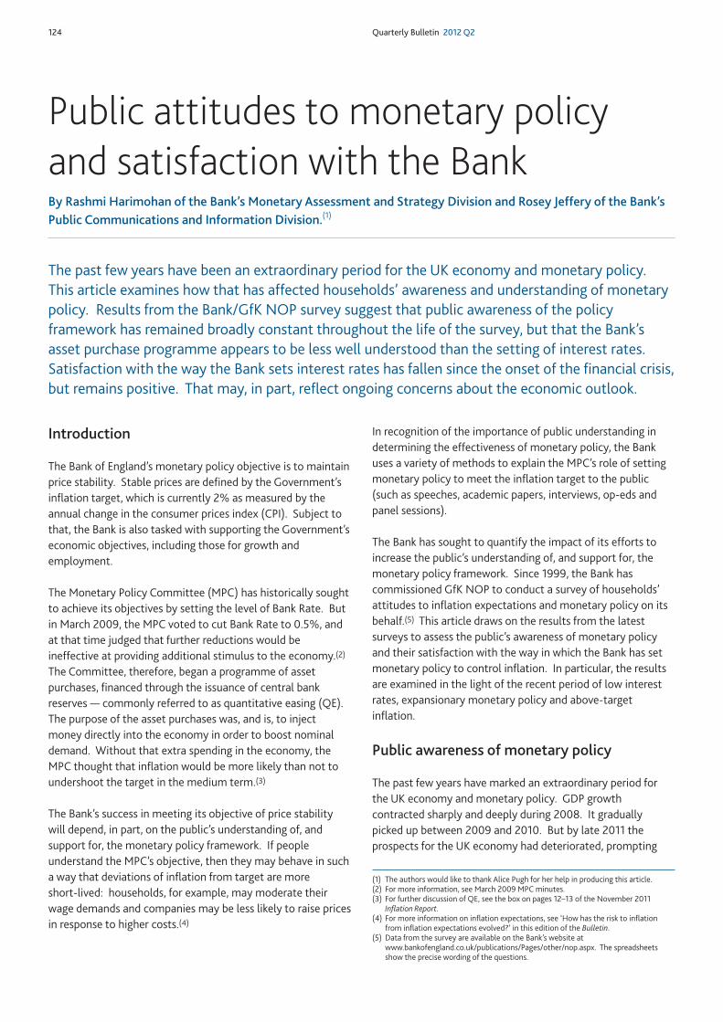
124 Quarterly Bulletin 2012 Q2
Introduction
The Bank of England’s monetary policy objective is to maintainprice stability. Stable prices are defined by the Government’sinflation target, which is currently 2% as measured by theannual change in the consumer prices index (CPI). Subject tothat, the Bank is also tasked with supporting the Government’seconomic objectives, including those for growth andemployment.
The Monetary Policy Committee (MPC) has historically soughtto achieve its objectives by setting the level of Bank Rate. Butin March 2009, the MPC voted to cut Bank Rate to 0.5%, andat that time judged that further reductions would beineffective at providing additional stimulus to the economy.(2)
The Committee, therefore, began a programme of assetpurchases, financed through the issuance of central bankreserves — commonly referred to as quantitative easing (QE).The purpose of the asset purchases was, and is, to injectmoney directly into the economy in order to boost nominaldemand. Without that extra spending in the economy, theMPC thought that inflation would be more likely than not toundershoot the target in the medium term.(3)
The Bank’s success in meeting its objective of price stabilitywill depend, in part, on the public’s understanding of, andsupport for, the monetary policy framework. If peopleunderstand the MPC’s objective, then they may behave in sucha way that deviations of inflation from target are more short-lived: households, for example, may moderate theirwage demands and companies may be less likely to raise pricesin response to higher costs.(4)
In recognition of the importance of public understanding indetermining the effectiveness of monetary policy, the Bankuses a variety of methods to explain the MPC’s role of settingmonetary policy to meet the inflation target to the public(such as speeches, academic papers, interviews, op-eds andpanel sessions).
The Bank has sought to quantify the impact of its efforts toincrease the public’s understanding of, and support for, themonetary policy framework. Since 1999, the Bank hascommissioned GfK NOP to conduct a survey of households’attitudes to inflation expectations and monetary policy on itsbehalf.(5) This article draws on the results from the latestsurveys to assess the public’s awareness of monetary policyand their satisfaction with the way in which the Bank has setmonetary policy to control inflation. In particular, the resultsare examined in the light of the recent period of low interestrates, expansionary monetary policy and above-targetinflation.
Public awareness of monetary policy
The past few years have marked an extraordinary period forthe UK economy and monetary policy. GDP growthcontracted sharply and deeply during 2008. It graduallypicked up between 2009 and 2010. But by late 2011 theprospects for the UK economy had deteriorated, prompting
The past few years have been an extraordinary period for the UK economy and monetary policy.This article examines how that has affected households’ awareness and understanding of monetarypolicy. Results from the Bank/GfK NOP survey suggest that public awareness of the policyframework has remained broadly constant throughout the life of the survey, but that the Bank’sasset purchase programme appears to be less well understood than the setting of interest rates.Satisfaction with the way the Bank sets interest rates has fallen since the onset of the financial crisis,but remains positive. That may, in part, reflect ongoing concerns about the economic outlook.
Public attitudes to monetary policy and satisfaction with the BankBy Rashmi Harimohan of the Bank’s Monetary Assessment and Strategy Division and Rosey Jeffery of the Bank’sPublic Communications and Information Division.(1)
(1) The authors would like to thank Alice Pugh for her help in producing this article.(2) For more information, see March 2009 MPC minutes.(3) For further discussion of QE, see the box on pages 12–13 of the November 2011
Inflation Report.(4) For more information on inflation expectations, see ‘How has the risk to inflation
from inflation expectations evolved?’ in this edition of the Bulletin.(5) Data from the survey are available on the Bank’s website at
www.bankofengland.co.uk/publications/Pages/other/nop.aspx. The spreadsheetsshow the precise wording of the questions.
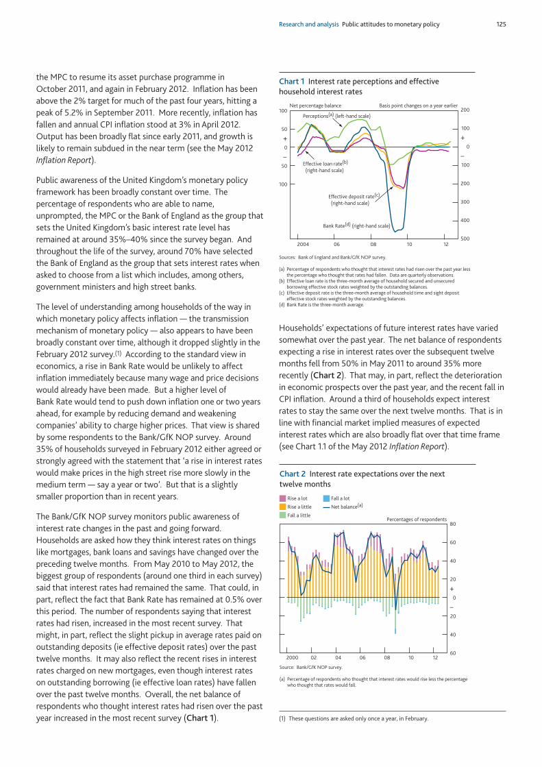
Research and analysis Public attitudes to monetary policy 125
the MPC to resume its asset purchase programme in October 2011, and again in February 2012. Inflation has beenabove the 2% target for much of the past four years, hitting apeak of 5.2% in September 2011. More recently, inflation hasfallen and annual CPI inflation stood at 3% in April 2012.Output has been broadly flat since early 2011, and growth islikely to remain subdued in the near term (see the May 2012 Inflation Report).
Public awareness of the United Kingdom’s monetary policyframework has been broadly constant over time. Thepercentage of respondents who are able to name,unprompted, the MPC or the Bank of England as the group thatsets the United Kingdom’s basic interest rate level hasremained at around 35%–40% since the survey began. Andthroughout the life of the survey, around 70% have selectedthe Bank of England as the group that sets interest rates whenasked to choose from a list which includes, among others,government ministers and high street banks.
The level of understanding among households of the way inwhich monetary policy affects inflation — the transmissionmechanism of monetary policy — also appears to have beenbroadly constant over time, although it dropped slightly in theFebruary 2012 survey.(1) According to the standard view ineconomics, a rise in Bank Rate would be unlikely to affectinflation immediately because many wage and price decisionswould already have been made. But a higher level of Bank Rate would tend to push down inflation one or two yearsahead, for example by reducing demand and weakeningcompanies’ ability to charge higher prices. That view is sharedby some respondents to the Bank/GfK NOP survey. Around35% of households surveyed in February 2012 either agreed orstrongly agreed with the statement that ‘a rise in interest rateswould make prices in the high street rise more slowly in themedium term — say a year or two’. But that is a slightlysmaller proportion than in recent years.
The Bank/GfK NOP survey monitors public awareness ofinterest rate changes in the past and going forward.Households are asked how they think interest rates on thingslike mortgages, bank loans and savings have changed over thepreceding twelve months. From May 2010 to May 2012, thebiggest group of respondents (around one third in each survey)said that interest rates had remained the same. That could, inpart, reflect the fact that Bank Rate has remained at 0.5% overthis period. The number of respondents saying that interestrates had risen, increased in the most recent survey. Thatmight, in part, reflect the slight pickup in average rates paid onoutstanding deposits (ie effective deposit rates) over the pasttwelve months. It may also reflect the recent rises in interestrates charged on new mortgages, even though interest rateson outstanding borrowing (ie effective loan rates) have fallenover the past twelve months. Overall, the net balance ofrespondents who thought interest rates had risen over the pastyear increased in the most recent survey (Chart 1).
Households’ expectations of future interest rates have variedsomewhat over the past year. The net balance of respondentsexpecting a rise in interest rates over the subsequent twelvemonths fell from 50% in May 2011 to around 35% morerecently (Chart 2). That may, in part, reflect the deteriorationin economic prospects over the past year, and the recent fall inCPI inflation. Around a third of households expect interestrates to stay the same over the next twelve months. That is inline with financial market implied measures of expectedinterest rates which are also broadly flat over that time frame(see Chart 1.1 of the May 2012 Inflation Report).
100
50
0
50
100
500
400
300
200
100
0
100
200
2004 06 08 10 12
Basis point changes on a year earlier Net percentage balance
Bank Rate(d) (right-hand scale)
Perceptions(a) (left-hand scale)
Effective deposit rate(c)
(right-hand scale)
Effective loan rate(b)
(right-hand scale)
+
–
+
–
Sources: Bank of England and Bank/GfK NOP survey.
(a) Percentage of respondents who thought that interest rates had risen over the past year lessthe percentage who thought that rates had fallen. Data are quarterly observations.
(b) Effective loan rate is the three-month average of household secured and unsecuredborrowing effective stock rates weighted by the outstanding balances.
(c) Effective deposit rate is the three-month average of household time and sight depositeffective stock rates weighted by the outstanding balances.
(d) Bank Rate is the three-month average.
Chart 1 Interest rate perceptions and effectivehousehold interest rates
(1) These questions are asked only once a year, in February.
60
40
20
0
20
40
60
80
2000 02 04 06 08 10 12
Rise a little
Rise a lot
Fall a little
Fall a lot
Net balance(a)
Percentages of respondents
+
–
Source: Bank/GfK NOP survey.
(a) Percentage of respondents who thought that interest rates would rise less the percentagewho thought that rates would fall.
Chart 2 Interest rate expectations over the nexttwelve months
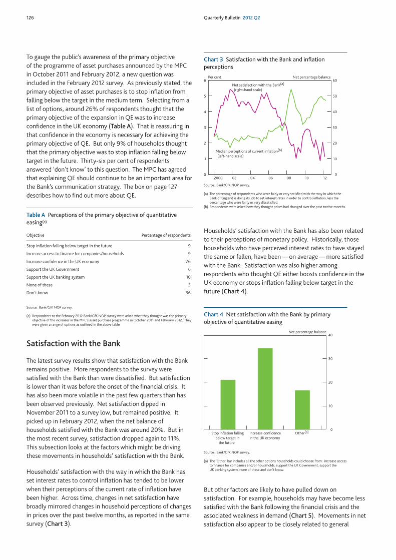
126 Quarterly Bulletin 2012 Q2
To gauge the public’s awareness of the primary objective of the programme of asset purchases announced by the MPCin October 2011 and February 2012, a new question wasincluded in the February 2012 survey. As previously stated, theprimary objective of asset purchases is to stop inflation fromfalling below the target in the medium term. Selecting from alist of options, around 26% of respondents thought that theprimary objective of the expansion in QE was to increaseconfidence in the UK economy (Table A). That is reassuring inthat confidence in the economy is necessary for achieving theprimary objective of QE. But only 9% of households thoughtthat the primary objective was to stop inflation falling belowtarget in the future. Thirty-six per cent of respondentsanswered ‘don’t know’ to this question. The MPC has agreedthat explaining QE should continue to be an important area forthe Bank’s communication strategy. The box on page 127describes how to find out more about QE.
Satisfaction with the Bank
The latest survey results show that satisfaction with the Bankremains positive. More respondents to the survey weresatisfied with the Bank than were dissatisfied. But satisfactionis lower than it was before the onset of the financial crisis. Ithas also been more volatile in the past few quarters than hasbeen observed previously. Net satisfaction dipped inNovember 2011 to a survey low, but remained positive. Itpicked up in February 2012, when the net balance ofhouseholds satisfied with the Bank was around 20%. But inthe most recent survey, satisfaction dropped again to 11%.This subsection looks at the factors which might be drivingthese movements in households’ satisfaction with the Bank.
Households’ satisfaction with the way in which the Bank hasset interest rates to control inflation has tended to be lowerwhen their perceptions of the current rate of inflation havebeen higher. Across time, changes in net satisfaction havebroadly mirrored changes in household perceptions of changesin prices over the past twelve months, as reported in the samesurvey (Chart 3).
Households’ satisfaction with the Bank has also been relatedto their perceptions of monetary policy. Historically, thosehouseholds who have perceived interest rates to have stayedthe same or fallen, have been — on average — more satisfiedwith the Bank. Satisfaction was also higher amongrespondents who thought QE either boosts confidence in theUK economy or stops inflation falling below target in thefuture (Chart 4).
But other factors are likely to have pulled down onsatisfaction. For example, households may have become lesssatisfied with the Bank following the financial crisis and theassociated weakness in demand (Chart 5). Movements in netsatisfaction also appear to be closely related to general
0
10
20
30
40
Stop inflation falling
below target in
the future
Increase confidence
in the UK economy
Other(a)
Net percentage balance
Source: Bank/GfK NOP survey.
(a) The ‘Other’ bar includes all the other options households could choose from: increase accessto finance for companies and/or households, support the UK Government, support the UK banking system, none of these and don’t know.
Chart 4 Net satisfaction with the Bank by primaryobjective of quantitative easing
Table A Perceptions of the primary objective of quantitativeeasing(a)
Objective Percentage of respondents
Stop inflation falling below target in the future 9
Increase access to finance for companies/households 9
Increase confidence in the UK economy 26
Support the UK Government 6
Support the UK banking system 10
None of these 5
Don’t know 36
Source: Bank/GfK NOP survey.
(a) Respondents to the February 2012 Bank/GfK NOP survey were asked what they thought was the primaryobjective of the increases in the MPC’s asset purchase programme in October 2011 and February 2012. Theywere given a range of options as outlined in the above table.
0
1
2
3
4
5
6
0
10
20
30
40
50
60
2000 02 04 06 08 10 12
Net satisfaction with the Bank(a)
(right-hand scale)
Net percentage balance Per cent
Median perceptions of current inflation(b)
(left-hand scale)
Source: Bank/GfK NOP survey.
(a) The percentage of respondents who were fairly or very satisfied with the way in which theBank of England is doing its job to set interest rates in order to control inflation, less thepercentage who were fairly or very dissatisfied.
(b) Respondents were asked how they thought prices had changed over the past twelve months.
Chart 3 Satisfaction with the Bank and inflationperceptions
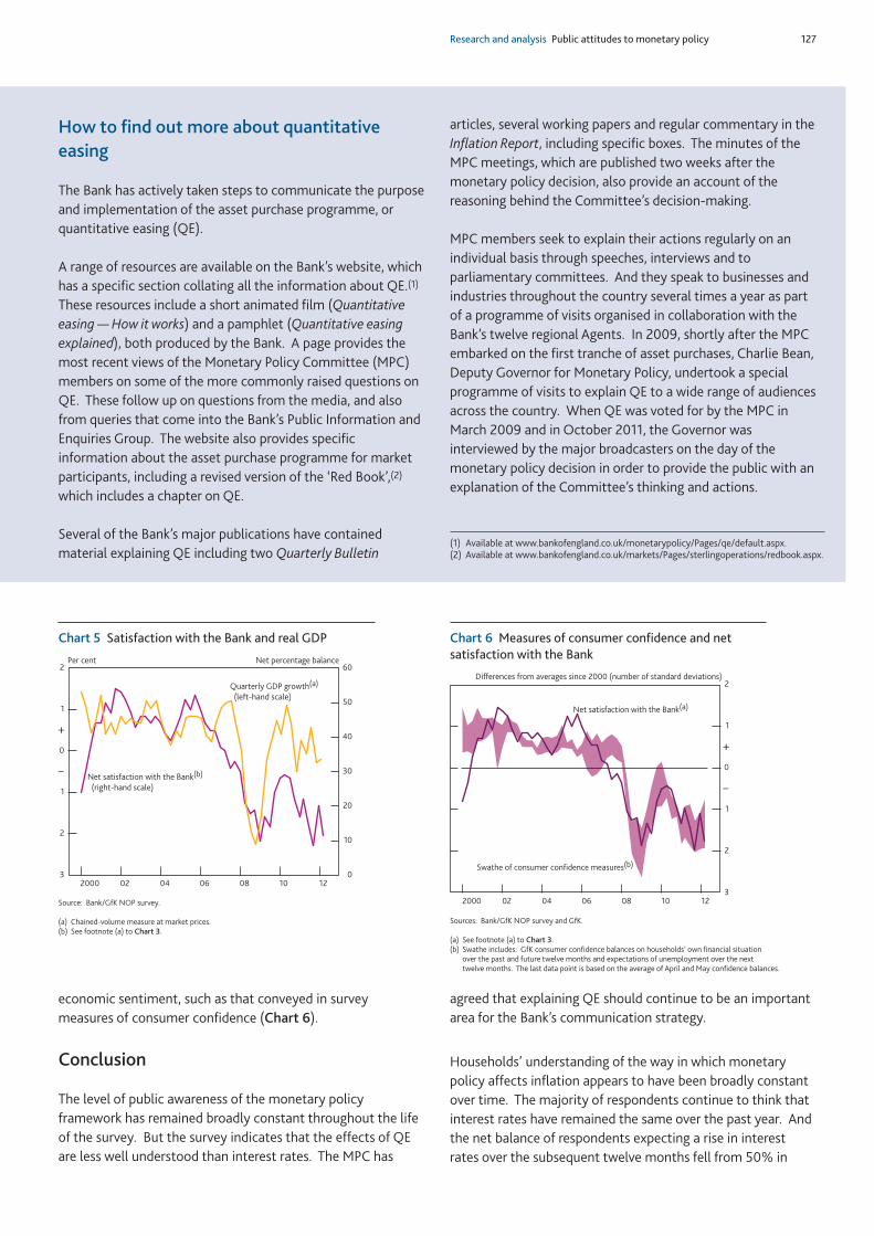
Research and analysis Public attitudes to monetary policy 127
economic sentiment, such as that conveyed in surveymeasures of consumer confidence (Chart 6).
Conclusion
The level of public awareness of the monetary policyframework has remained broadly constant throughout the lifeof the survey. But the survey indicates that the effects of QEare less well understood than interest rates. The MPC has
agreed that explaining QE should continue to be an importantarea for the Bank’s communication strategy.
Households’ understanding of the way in which monetarypolicy affects inflation appears to have been broadly constantover time. The majority of respondents continue to think thatinterest rates have remained the same over the past year. Andthe net balance of respondents expecting a rise in interestrates over the subsequent twelve months fell from 50% in
3
2
1
0
1
2
2000 02 04 06 08 10 12
Net satisfaction with the Bank(a)
Differences from averages since 2000 (number of standard deviations)
Swathe of consumer confidence measures(b)
+
–
Sources: Bank/GfK NOP survey and GfK.
(a) See footnote (a) to Chart 3.(b) Swathe includes: GfK consumer confidence balances on households’ own financial situation
over the past and future twelve months and expectations of unemployment over the next twelve months. The last data point is based on the average of April and May confidence balances.
Chart 6 Measures of consumer confidence and netsatisfaction with the Bank
3
2
1
0
1
2
0
10
20
30
40
50
60
2000 02 04 06 08 10 12
Net satisfaction with the Bank(b)
(right-hand scale)
Net percentage balance Per cent
Quarterly GDP growth(a)
(left-hand scale)
+
–
Source: Bank/GfK NOP survey.
(a) Chained-volume measure at market prices. (b) See footnote (a) to Chart 3.
Chart 5 Satisfaction with the Bank and real GDP
How to find out more about quantitativeeasing
The Bank has actively taken steps to communicate the purposeand implementation of the asset purchase programme, orquantitative easing (QE).
A range of resources are available on the Bank’s website, whichhas a specific section collating all the information about QE.(1)
These resources include a short animated film (Quantitativeeasing — How it works) and a pamphlet (Quantitative easingexplained), both produced by the Bank. A page provides themost recent views of the Monetary Policy Committee (MPC)members on some of the more commonly raised questions onQE. These follow up on questions from the media, and alsofrom queries that come into the Bank’s Public Information andEnquiries Group. The website also provides specificinformation about the asset purchase programme for marketparticipants, including a revised version of the ‘Red Book’,(2)
which includes a chapter on QE.
Several of the Bank’s major publications have containedmaterial explaining QE including two Quarterly Bulletin
articles, several working papers and regular commentary in theInflation Report, including specific boxes. The minutes of theMPC meetings, which are published two weeks after themonetary policy decision, also provide an account of thereasoning behind the Committee’s decision-making.
MPC members seek to explain their actions regularly on anindividual basis through speeches, interviews and toparliamentary committees. And they speak to businesses andindustries throughout the country several times a year as partof a programme of visits organised in collaboration with theBank’s twelve regional Agents. In 2009, shortly after the MPCembarked on the first tranche of asset purchases, Charlie Bean,Deputy Governor for Monetary Policy, undertook a specialprogramme of visits to explain QE to a wide range of audiencesacross the country. When QE was voted for by the MPC inMarch 2009 and in October 2011, the Governor wasinterviewed by the major broadcasters on the day of themonetary policy decision in order to provide the public with anexplanation of the Committee’s thinking and actions.
(1) Available at www.bankofengland.co.uk/monetarypolicy/Pages/qe/default.aspx.(2) Available at www.bankofengland.co.uk/markets/Pages/sterlingoperations/redbook.aspx.

128 Quarterly Bulletin 2012 Q2
May 2011 to around 35% more recently. A similar proportionof households expect interest rates to stay the same over thenext twelve months. That is in line with financial marketimplied measures of expected interest rates.
Satisfaction with the way in which the Bank has set interestrates to control inflation has fallen since the financial crisis, but
remains positive. It has also been more volatile in the past fewquarters than has been observed previously. Following asurvey low for satisfaction in November 2011, the net balancepicked up in February 2012, but dipped again in May 2012.That may, in part, reflect ongoing concerns about theeconomic outlook.
Research and analysis The impact of QE on gilt yields 129
In March 2009, the Bank of England announced that itwould begin a programme of large-scale asset purchasesfinanced using central bank money; a policy widely referredto as quantitative easing (QE). By May 2012 the Bank’spurchases totalled £325 billion, almost exclusively in UKgovernment bonds (gilts). The aim of asset purchases isconceptually the same as a cut in Bank Rate: to stimulatenominal spending in order to meet the 2% inflation target inthe medium term.
There are a number of channels through which asset purchasesmight affect spending and inflation.(2) The first leg of many ofthese channels is the impact of asset purchases on gilt yields:purchases by the Bank increase the price of gilts and thereforelower their yields. But identifying this impact on yields hasbecome increasingly difficult as financial markets have begunto anticipate future purchases. This article uses a novelapproach to isolate part of the impact of QE on gilt yields, byusing ‘natural experiments’ associated with operationalchanges that contained news about the distribution of futuregilt purchases.
Given that financial markets are forward looking, the majorityof the impact of asset purchases on gilt yields is likely to occurwhen expectations of purchases are formed — rather thanwhen the purchases are actually made.(3) Therefore changes ingilt yields will be observed when there is ‘news’ that changesexpectations about future purchases.
When QE was first introduced, the policy was unfamiliar tofinancial market participants. So it is likely that theirexpectations of the size of asset purchases were formedprimarily from Monetary Policy Committee (MPC)announcements about the planned amount of QE purchases.Therefore these initial announcements contained significantnews and so could be used to estimate the effect of QE ongilt yields.
Over time, however, gilt market participants have learned howthe MPC’s QE decisions depend on the United Kingdom’seconomic outlook. Expectations of gilt purchases aretherefore increasingly formed when economic news and dataare released, that is, in advance of the MPC announcementitself. Subsequent MPC announcements have thus containedless news about gilt purchases, making it harder to identify theimpact of QE on gilt yields from the immediate marketreaction to these announcements. Just as with changes inBank Rate, expectations of policy changes which are alreadywidely anticipated will have little market impact when they areactually announced.
Using the information contained in economic news and data releases, financial markets have widelyanticipated recent Monetary Policy Committee announcements about the amount of assets theBank of England intends to purchase as part of its quantitative easing (QE) policy. This makes itincreasingly difficult to identify the impact of QE on gilt yields. This article uses three ‘naturalexperiments’ associated with operational changes to the distribution of gilt purchases — in March 2009, August 2009 and February 2012 — to help overcome this identification problem. Itfinds that the ‘local supply’ channel, which can be identified using these events, can explain aroundhalf of the total impact of QE on gilt yields. The estimates of this effect are broadly similar acrossthe three events; so the strength of this channel of QE does not appear to have changedsignificantly since gilt purchases were introduced in early 2009.
Using changes in auction maturitysectors to help identify the impact ofQE on gilt yieldsBy Ryan Banerjee, David Latto and Nick McLaren of the Bank’s Macro Financial Analysis Division and Sebastiano Daros of the Bank’s Sterling Markets Division.(1)
(1) The authors would like to thank Michael Chin and Zhuoshi Liu for their help inproducing this article.
(2) For a more detailed discussion see the previous Quarterly Bulletin article by Joyce,Tong and Woods (2011).
(3) Forthcoming work by Daines, Joyce and Tong (2012) finds that there may have been some impact on yields at the time of purchases during the early stages of QE purchases in 2009. But the majority of the impact was observed when purchaseswere announced.
130 Quarterly Bulletin 2012 Q2
This article tries to overcome this identification problem byusing the reaction of gilt yields to market notices whichcontained operational changes to the distribution of giltpurchases that were largely unanticipated. These notices areunlikely to have changed the total amount of gilt purchasesmarket participants were expecting the Bank to make in thefuture. But the notices did have implications for how theseexpected purchases were likely to be spread across differentgroups of gilts. Therefore these events can be used todetermine how each gilt’s yield changes given a change in theamount of that gilt that is expected to be purchased. Althoughthis does not capture all of the effects of QE on gilt yields, itcan help to identify a part of the effect. Furthermore, becausethe timings of these notices (in March 2009, August 2009 andFebruary 2012) span the period of QE purchases, they can alsobe used to determine if the strength of this effect has changedover time.
The first section of this article outlines the channels throughwhich asset purchases affect gilt yields, and discusses which ofthese can be identified using these natural experiments. Thesecond section explains how the news in the operationalmarket notices can be quantified. The third section uses aregression approach to investigate the link between thismeasure of news and the change in yields, to help quantify thispart of the impact of QE. The fourth section puts the resultsinto context by comparing them to other work on QE for theUnited Kingdom and the United States. The final sectionconcludes.
Channels from QE to gilt yields
This section outlines the links between QE and gilt yields,and then explains which of these channels can be identifiedusing the operational market notice events. The link betweenQE and gilt yields is usually explained by the following effects:
• Local supply: if some investors do not view gilts of differentmaturities as perfect substitutes (for example, someinvestors will strongly prefer to hold longer-maturity assetsto match their long-dated liabilities) then central bankpurchases expected in a specific maturity range can reducethe remaining supply of gilts expected to be available toprivate sector participants, driving up prices and loweringyields in that part of the yield curve.(1)
• Duration:(2) if the marginal investor in the market dislikesthe risk associated with holding long-maturity assets, thenmarket prices will contain a ‘term premium’ which will, inpart, compensate the holder for bearing this ‘duration risk’.Purchases of long-maturity assets, such as long-dated gilts,by the central bank will reduce the aggregate amount of thisduration risk remaining in the private market. This reducesthe compensation required for investors to hold theremaining bonds. As a result each gilt’s term premium will
fall, with the extent of the fall increasing with the maturityof the gilt.
• Interest rate signalling: QE announcements may conveyinformation about the central bank’s view of the economyand so the likely future path of Bank Rate. This news aboutthe path of short-term interest rates would be expected to have a larger impact on shorter-maturity gilts thanlonger-maturity gilts.
• Liquidity: the presence of the central bank in the gilt marketas a buyer may provide a ‘backstop’ which improves marketfunctioning and increases liquidity. This reduces the cost oftrading bonds, and so will reduce the ‘illiquidity premium’demanded to compensate investors for holding theremaining bonds.
As noted, the market notices contained news about the wayexpected purchases would be distributed across different gilts.This would have changed expectations of both the local supplyof gilts and the aggregate amount of duration risk remaining inthe private market. It is unlikely, however, that the marketnotices would have signalled anything about the path ofBank Rate; and given the size and depth of the gilt market, it isalso unlikely that overall market liquidity would have changedgreatly. This suggests the market notices might be useful inhelping to identify local supply and duration effects.
But while it is possible to estimate the local supply effects, it isnot possible to identify the duration effects. The difficulty isthat market notices were released on the same day as MPCannouncements about the total planned amount of assetpurchases. It is possible to take this into account whenestimating the local supply effects. But these announcementsmay also have been interpreted as signalling a change to theexpected path of Bank Rate, for instance that interest rateswould remain lower for a longer period. Such signalling effectscannot be distinguished from the effect of the announcementson duration risk. This is because both of these effects varymonotonically depending on the maturity of the gilt: durationrisk effects are smoothly increasing with maturity and interestrate signalling effects are smoothly decreasing with maturity.So it is difficult to distinguish the variation due to each effect.Fortunately, it is possible to control for the joint effect of thesechannels, so the market notice announcements can still beused to isolate the local supply effects.
(1) In theory, these differences may be short-lived if other market participants withoutsuch preferences are able to exploit arbitrage opportunities across bonds of differentmaturities. But if there are some constraints on arbitrageurs’ ability to bear risk, thenthese differences can persist.
(2) Duration is a measure of the remaining maturity of a bond which also takes intoaccount the time profile of coupon payments associated with the bond. For atheoretical model incorporating this channel, see Vayanos and Vila (2009).
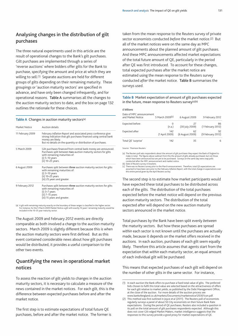
Research and analysis The impact of QE on gilt yields 131
Analysing changes in the distribution of giltpurchases
The three natural experiments used in this article are the result of operational changes to the Bank’s gilt purchases. Gilt purchases are implemented through a series of ‘reverse auctions’ where bidders offer gilts for the Bank topurchase, specifying the amount and price at which they arewilling to sell.(1) Separate auctions are held for differentgroups of gilts depending on their remaining maturity. Thesegroupings or ‘auction maturity sectors’ are specified inadvance, and have only been changed infrequently, and foroperational reasons. Table A summarises all the changes tothe auction maturity sectors to date, and the box on page 132outlines the rationale for these choices.
The August 2009 and February 2012 events are directlycomparable as both involved a change to the auction maturitysectors. March 2009 is slightly different because this is whenthe auction maturity sectors were first defined. But as thisevent contained considerable news about how gilt purchaseswould be distributed, it provides a useful comparison to theother two events.
Quantifying the news in operational marketnotices
To assess the reaction of gilt yields to changes in the auctionmaturity sectors, it is necessary to calculate a measure of thenews contained in the market notices. For each gilt, this is thedifference between expected purchases before and after themarket notice.
The first step is to estimate expectations of total future QEpurchases, before and after the market notice. The former is
taken from the mean response to the Reuters survey of privatesector economists conducted before the market notice.(2) Butall of the market notices were on the same day as MPCannouncements about the planned amount of gilt purchases.And these MPC announcements affected market expectationsof the total future amount of QE, particularly in the periodafter QE was first introduced. To account for these changes,total expected purchases after the market notice areestimated using the mean response to the Reuters surveyconducted after the market notice. Table B summarises thesurveys used.
The second step is to estimate how market participants wouldhave expected these total purchases to be distributed acrosseach of the gilts. The distribution of the total purchasesexpected before the market notice will depend on the previousauction maturity sectors. The distribution of the totalexpected after will depend on the new auction maturitysectors announced in the market notice.
Total purchases by the Bank have been split evenly betweenthe maturity sectors. But how these purchases are spreadwithin each sector is not known until the purchases are actuallymade, because it depends on the market offers received in theauctions. In each auction, purchases of each gilt seem equallylikely. Therefore this article assumes that agents start from theexpectation that within each maturity sector, an equal amountof each individual gilt will be purchased.
This means that expected purchases of each gilt will depend onthe number of other gilts in the same sector. For instance,
(1) In each auction the Bank offers to purchase a fixed total value of gilts. The preferredbids chosen to fulfil this total value are selected based on the attractiveness of offersfor each gilt relative to market yields, as published by the Debt Management Office,at the close of the auction. For more details of the auction process seewww.bankofengland.co.uk/markets/Documents/marketnotice120301con.pdf.
(2) This method was first outlined in Joyce et al (2011). The Reuters poll of economistsregularly surveys a panel of about 50 City economists on their future Bank Rateexpectations. During the period of QE purchases, Reuters also included a question inits poll on the total amount of gilt purchases respondents expected. Although thisdoes not cover Gilt-edged Market Makers, market intelligence suggests that theresponses to this survey provide a good proxy for market expectations of QE.
Table A Changes in auction maturity sectors(a)
Market Notice Auction details
11 February 2009 February Inflation Report and associated press conference give strong indication that gilt purchases financed using central bank money are likely. But no details on the quantity or distribution of purchases.
5 March 2009 Gilt purchases financed from central bank money are announced.Purchases split between two auction maturity sectors for gilts with remaining maturities of:(i) 5–10 years (ii) 10–25 years.
6 August 2009 Purchases split between three auction maturity sectors for gilts with remaining maturities of: (i) 3–10 years (ii) 10–25 years (iii) 25 years and greater.
9 February 2012 Purchases split between three auction maturity sectors for gilts with remaining maturities of: (i) 3–7 years (ii) 7–15 years (iii) 15 years and greater.
(a) A gilt with remaining maturity exactly on the boundary of these ranges is classified in the higher sector.For instance, for the 5 March 2009 Market Notice a gilt with exactly 10 years’ remaining maturity would beincluded in the 10–25 year maturity sector.
Table B Market expectation of amount of gilt purchases expectedin the future, mean response to Reuters survey(a)(b)
£ billions
Date of MPC announcementand Market Notice 5 March 2009(c) 6 August 2009 9 February 2012
Expected before 0 27 86(n.a.) (30 July 2009) (1 February 2012)
Expected after 142 62 92(1 April 2009) (6 August 2009) (9 February 2012)
Total QE ‘surprise’ 142 35 6
Source: Thomson Reuters.
(a) The Reuters poll asks respondents about the amount of gilt purchases they expect the Bank of England tomake in total. The figures above subtract from this the amount of gilts already purchased, but not thosewhich have been announced but are yet to be purchased. Surveys on the same day were snap pollsconducted after the MPC announcement and market notice.
(b) Date of Reuters survey in brackets.(c) There was no Reuters survey prior to the March announcement. Therefore, total QE expectations are
assumed to have been zero prior to the February Inflation Report, with the total change in expectations overthis entire period given by the April Reuters survey.
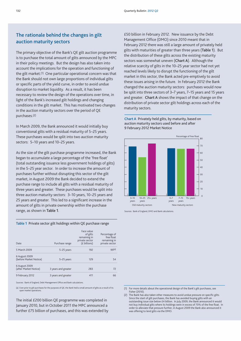
132 Quarterly Bulletin 2012 Q2
The rationale behind the changes in giltauction maturity sectors
The primary objective of the Bank’s QE gilt auction programmeis to purchase the total amount of gilts announced by the MPCin their policy meetings. But the design has also taken intoaccount the implications for the operation and functioning ofthe gilt market.(1) One particular operational concern was thatthe Bank should not own large proportions of individual giltsor specific parts of the yield curve, in order to avoid unduedisruption to market liquidity. As a result, it has beennecessary to review the design of the operations over time, inlight of the Bank’s increased gilt holdings and changingconditions in the gilt market. This has motivated two changesin the auction maturity sectors over the period of QEpurchases.(2)
In March 2009, the Bank announced it would initially buyconventional gilts with a residual maturity of 5–25 years.These purchases would be split into two auction maturitysectors: 5–10 years and 10–25 years.
As the size of the gilt purchase programme increased, the Bankbegan to accumulate a large percentage of the ‘free float’(total outstanding issuance less government holdings of gilts)in the 5–25 year sector. In order to increase the amount ofpurchases further without disrupting this sector of the giltmarket, in August 2009 the Bank decided to extend thepurchase range to include all gilts with a residual maturity ofthree years and greater. These purchases would be split intothree auction maturity sectors: 3–10 years, 10–25 years and25 years and greater. This led to a significant increase in theamount of gilts in private ownership within the purchaserange, as shown in Table 1.
The initial £200 billion QE programme was completed inJanuary 2010, but in October 2011 the MPC announced afurther £75 billion of purchases, and this was extended by
£50 billion in February 2012. New issuance by the DebtManagement Office (DMO) since 2010 meant that inFebruary 2012 there was still a large amount of privately heldgilts with maturities of greater than three years (Table 1). Butthe distribution of these gilts across the existing maturitysectors was somewhat uneven (Chart A). Although therelative scarcity of gilts in the 10–25 year sector had not yetreached levels likely to disrupt the functioning of the giltmarket in this sector, the Bank acted pre-emptively to avoidthese issues arising in the future. In February 2012 the Bankchanged the auction maturity sectors: purchases would nowbe split into three sectors of 3–7 years, 7–15 years and 15 yearsand greater. Chart A shows the impact of that change on thedistribution of private sector gilt holdings across each of thematurity sectors.
0
10
20
30
40
50
60
70
80Percentage of free float
3–10
years
25+ years 15+ years
Old maturity sectors New maturity sectors
10–25
years
3–7
years
7–15
years
Chart A Privately held gilts, by maturity, based onauction maturity sectors used before and after 9 February 2012 Market Notice
Sources: Bank of England, DMO and Bank calculations.
(1) For more details about the operational design of the Bank’s gilt purchases, seeFisher (2010).
(2) The Bank has also taken other measures to avoid undue pressure on specific gilts.Since the start of gilt purchases, the Bank has avoided buying gilts with anoutstanding issue size below £4 billion. In July 2009, the Bank announced it wouldnot buy individual gilts where its holdings were in excess of 70% of the free float. Inorder to alleviate that pressure further, in August 2009 the Bank also announced itwas offering to lend gilts via the DMO.
Table 1 Private sector gilt holdings within QE purchase range
Face value of gilts Percentage of
remaining in free floatprivate sector remaining in
Date Purchase range (£ billions) private sector
5 March 2009 5–25 years 192 99(a)
6 August 2009 (before Market Notice) 5–25 years 129 54
6 August 2009 (after Market Notice) 3 years and greater 283 72
9 February 2012 3 years and greater 411 66
Sources: Bank of England, Debt Management Office and Bank calculations.
(a) Even prior to gilt purchases for the purposes of QE, the Bank held a small amount of gilts as a result of itsopen market operations.
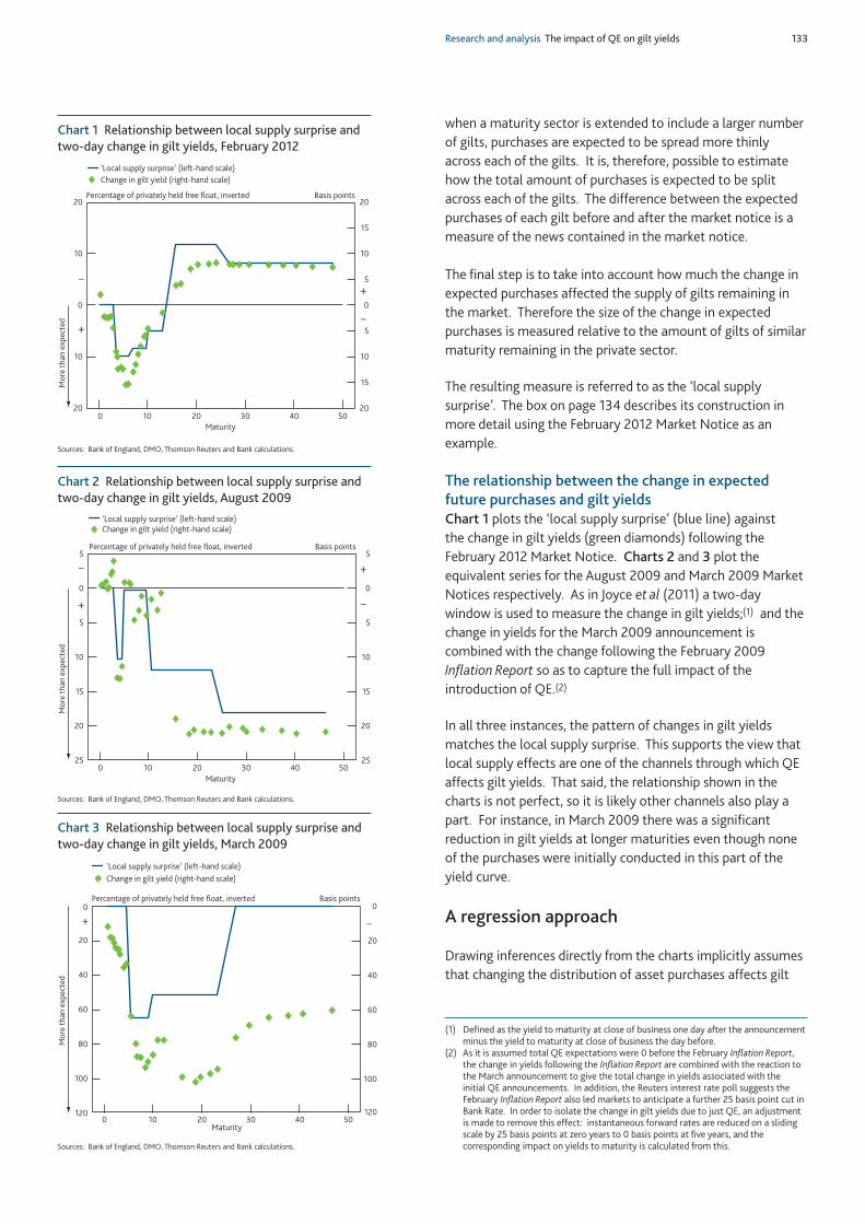
Research and analysis The impact of QE on gilt yields 133
when a maturity sector is extended to include a larger numberof gilts, purchases are expected to be spread more thinlyacross each of the gilts. It is, therefore, possible to estimatehow the total amount of purchases is expected to be splitacross each of the gilts. The difference between the expectedpurchases of each gilt before and after the market notice is ameasure of the news contained in the market notice.
The final step is to take into account how much the change inexpected purchases affected the supply of gilts remaining inthe market. Therefore the size of the change in expectedpurchases is measured relative to the amount of gilts of similarmaturity remaining in the private sector.
The resulting measure is referred to as the ‘local supplysurprise’. The box on page 134 describes its construction inmore detail using the February 2012 Market Notice as anexample.
The relationship between the change in expectedfuture purchases and gilt yieldsChart 1 plots the ‘local supply surprise’ (blue line) against the change in gilt yields (green diamonds) following theFebruary 2012 Market Notice. Charts 2 and 3 plot theequivalent series for the August 2009 and March 2009 MarketNotices respectively. As in Joyce et al (2011) a two-daywindow is used to measure the change in gilt yields;(1) and thechange in yields for the March 2009 announcement iscombined with the change following the February 2009Inflation Report so as to capture the full impact of theintroduction of QE.(2)
In all three instances, the pattern of changes in gilt yieldsmatches the local supply surprise. This supports the view thatlocal supply effects are one of the channels through which QEaffects gilt yields. That said, the relationship shown in thecharts is not perfect, so it is likely other channels also play apart. For instance, in March 2009 there was a significantreduction in gilt yields at longer maturities even though noneof the purchases were initially conducted in this part of theyield curve.
A regression approach
Drawing inferences directly from the charts implicitly assumesthat changing the distribution of asset purchases affects gilt
(1) Defined as the yield to maturity at close of business one day after the announcementminus the yield to maturity at close of business the day before.
(2) As it is assumed total QE expectations were 0 before the February Inflation Report,the change in yields following the Inflation Report are combined with the reaction tothe March announcement to give the total change in yields associated with the initial QE announcements. In addition, the Reuters interest rate poll suggests theFebruary Inflation Report also led markets to anticipate a further 25 basis point cut in Bank Rate. In order to isolate the change in gilt yields due to just QE, an adjustmentis made to remove this effect: instantaneous forward rates are reduced on a slidingscale by 25 basis points at zero years to 0 basis points at five years, and thecorresponding impact on yields to maturity is calculated from this.
20
15
10
5
0
5
10
15
20 20
10
0
10
20 0 10 20 30 40 50
Mo
re t
han
exp
ecte
d
‘Local supply surprise’ (left-hand scale)
Change in gilt yield (right-hand scale)
Basis points Percentage of privately held free float, inverted
Maturity
+
–
_
+
Chart 1 Relationship between local supply surprise andtwo-day change in gilt yields, February 2012
Sources: Bank of England, DMO, Thomson Reuters and Bank calculations.
25
20
15
10
5
0
5 5
0
5
10
15
20
25 0 10 20 30 40 50
‘Local supply surprise’ (left-hand scale)Change in gilt yield (right-hand scale)
Basis points Percentage of privately held free float, inverted
Maturity
–
+
+
–
Mo
re t
han
exp
ecte
d
Chart 2 Relationship between local supply surprise andtwo-day change in gilt yields, August 2009
Sources: Bank of England, DMO, Thomson Reuters and Bank calculations.
120
100
80
60
40
20
0 0
20
40
60
80
100
120 0 10 20 30 40 50
‘Local supply surprise’ (left-hand scale)
Basis points Percentage of privately held free float, inverted
Maturity
Change in gilt yield (right-hand scale)
_+
Mo
re t
han
exp
ecte
d
Chart 3 Relationship between local supply surprise andtwo-day change in gilt yields, March 2009
Sources: Bank of England, DMO, Thomson Reuters and Bank calculations.
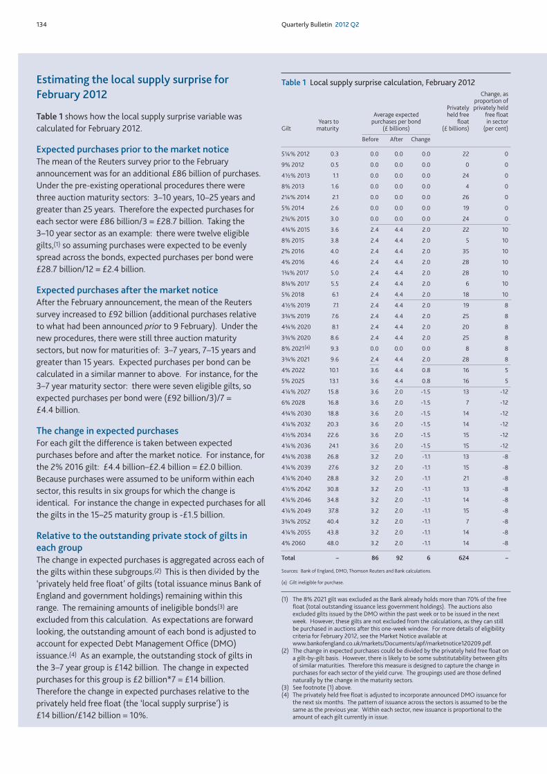
134 Quarterly Bulletin 2012 Q2
Estimating the local supply surprise forFebruary 2012
Table 1 shows how the local supply surprise variable wascalculated for February 2012.
Expected purchases prior to the market noticeThe mean of the Reuters survey prior to the Februaryannouncement was for an additional £86 billion of purchases.Under the pre-existing operational procedures there werethree auction maturity sectors: 3–10 years, 10–25 years andgreater than 25 years. Therefore the expected purchases foreach sector were £86 billion/3 = £28.7 billion. Taking the 3–10 year sector as an example: there were twelve eligiblegilts,(1) so assuming purchases were expected to be evenlyspread across the bonds, expected purchases per bond were £28.7 billion/12 = £2.4 billion.
Expected purchases after the market noticeAfter the February announcement, the mean of the Reuterssurvey increased to £92 billion (additional purchases relativeto what had been announced prior to 9 February). Under thenew procedures, there were still three auction maturitysectors, but now for maturities of: 3–7 years, 7–15 years andgreater than 15 years. Expected purchases per bond can becalculated in a similar manner to above. For instance, for the3–7 year maturity sector: there were seven eligible gilts, soexpected purchases per bond were (£92 billion/3)/7 = £4.4 billion.
The change in expected purchases For each gilt the difference is taken between expectedpurchases before and after the market notice. For instance, forthe 2% 2016 gilt: £4.4 billion–£2.4 billion = £2.0 billion.Because purchases were assumed to be uniform within eachsector, this results in six groups for which the change isidentical. For instance the change in expected purchases for allthe gilts in the 15–25 maturity group is -£1.5 billion.
Relative to the outstanding private stock of gilts ineach groupThe change in expected purchases is aggregated across each ofthe gilts within these subgroups.(2) This is then divided by the‘privately held free float’ of gilts (total issuance minus Bank ofEngland and government holdings) remaining within thisrange. The remaining amounts of ineligible bonds(3) areexcluded from this calculation. As expectations are forwardlooking, the outstanding amount of each bond is adjusted toaccount for expected Debt Management Office (DMO)issuance.(4) As an example, the outstanding stock of gilts inthe 3–7 year group is £142 billion. The change in expectedpurchases for this group is £2 billion*7 = £14 billion.Therefore the change in expected purchases relative to theprivately held free float (the ‘local supply surprise’) is£14 billion/£142 billion = 10%.
(1) The 8% 2021 gilt was excluded as the Bank already holds more than 70% of the freefloat (total outstanding issuance less government holdings). The auctions alsoexcluded gilts issued by the DMO within the past week or to be issued in the nextweek. However, these gilts are not excluded from the calculations, as they can stillbe purchased in auctions after this one-week window. For more details of eligibilitycriteria for February 2012, see the Market Notice available atwww.bankofengland.co.uk/markets/Documents/apf/marketnotice120209.pdf.
(2) The change in expected purchases could be divided by the privately held free float ona gilt-by-gilt basis. However, there is likely to be some substitutability between giltsof similar maturities. Therefore this measure is designed to capture the change inpurchases for each sector of the yield curve. The groupings used are those definednaturally by the change in the maturity sectors.
(3) See footnote (1) above.(4) The privately held free float is adjusted to incorporate announced DMO issuance for
the next six months. The pattern of issuance across the sectors is assumed to be thesame as the previous year. Within each sector, new issuance is proportional to theamount of each gilt currently in issue.
Table 1 Local supply surprise calculation, February 2012Change, as
proportion ofPrivately privately held
Average expected held free free floatYears to purchases per bond float in sector
Gilt maturity (£ billions) (£ billions) (per cent)
Before After Change
5¼% 2012 0.3 0.0 0.0 0.0 22 0
9% 2012 0.5 0.0 0.0 0.0 0 0
4½% 2013 1.1 0.0 0.0 0.0 24 0
8% 2013 1.6 0.0 0.0 0.0 4 0
2¼% 2014 2.1 0.0 0.0 0.0 26 0
5% 2014 2.6 0.0 0.0 0.0 19 0
2¾% 2015 3.0 0.0 0.0 0.0 24 0
4¾% 2015 3.6 2.4 4.4 2.0 22 10
8% 2015 3.8 2.4 4.4 2.0 5 10
2% 2016 4.0 2.4 4.4 2.0 35 10
4% 2016 4.6 2.4 4.4 2.0 28 10
1¾% 2017 5.0 2.4 4.4 2.0 28 10
8¾% 2017 5.5 2.4 4.4 2.0 6 10
5% 2018 6.1 2.4 4.4 2.0 18 10
4½% 2019 7.1 2.4 4.4 2.0 19 8
3¾% 2019 7.6 2.4 4.4 2.0 25 8
4¾% 2020 8.1 2.4 4.4 2.0 20 8
3¾% 2020 8.6 2.4 4.4 2.0 25 8
8% 2021(a) 9.3 0.0 0.0 0.0 8 8
3¾% 2021 9.6 2.4 4.4 2.0 28 8
4% 2022 10.1 3.6 4.4 0.8 16 5
5% 2025 13.1 3.6 4.4 0.8 16 5
4¼% 2027 15.8 3.6 2.0 -1.5 13 -12
6% 2028 16.8 3.6 2.0 -1.5 7 -12
4¾% 2030 18.8 3.6 2.0 -1.5 14 -12
4¼% 2032 20.3 3.6 2.0 -1.5 14 -12
4½% 2034 22.6 3.6 2.0 -1.5 15 -12
4¼% 2036 24.1 3.6 2.0 -1.5 15 -12
4¾% 2038 26.8 3.2 2.0 -1.1 13 -8
4¼% 2039 27.6 3.2 2.0 -1.1 15 -8
4¼% 2040 28.8 3.2 2.0 -1.1 21 -8
4½% 2042 30.8 3.2 2.0 -1.1 13 -8
4¼% 2046 34.8 3.2 2.0 -1.1 14 -8
4¼% 2049 37.8 3.2 2.0 -1.1 15 -8
3¾% 2052 40.4 3.2 2.0 -1.1 7 -8
4¼% 2055 43.8 3.2 2.0 -1.1 14 -8
4% 2060 48.0 3.2 2.0 -1.1 14 -8
Total – 86 92 6 624 –
Sources: Bank of England, DMO, Thomson Reuters and Bank calculations.
(a) Gilt ineligible for purchase.
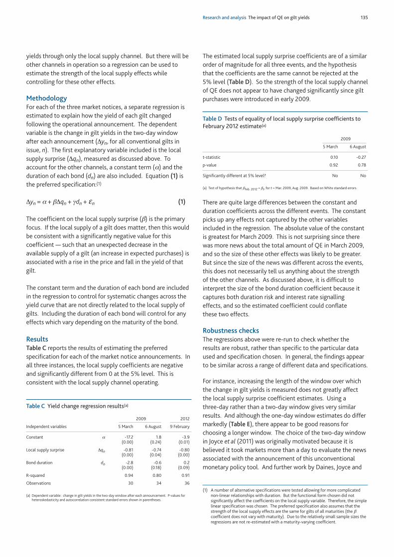
Research and analysis The impact of QE on gilt yields 135
yields through only the local supply channel. But there will beother channels in operation so a regression can be used toestimate the strength of the local supply effects whilecontrolling for these other effects.
MethodologyFor each of the three market notices, a separate regression isestimated to explain how the yield of each gilt changedfollowing the operational announcement. The dependentvariable is the change in gilt yields in the two-day windowafter each announcement (Δyn, for all conventional gilts inissue, n). The first explanatory variable included is the localsupply surprise (Δqn), measured as discussed above. Toaccount for the other channels, a constant term (α) and theduration of each bond (dn) are also included. Equation (1) isthe preferred specification:(1)
Δyn = α + βΔqn + γdn + εn (1)
The coefficient on the local supply surprise (β) is the primaryfocus. If the local supply of a gilt does matter, then this wouldbe consistent with a significantly negative value for thiscoefficient — such that an unexpected decrease in theavailable supply of a gilt (an increase in expected purchases) isassociated with a rise in the price and fall in the yield of thatgilt.
The constant term and the duration of each bond are includedin the regression to control for systematic changes across theyield curve that are not directly related to the local supply ofgilts. Including the duration of each bond will control for anyeffects which vary depending on the maturity of the bond.
ResultsTable C reports the results of estimating the preferredspecification for each of the market notice announcements. Inall three instances, the local supply coefficients are negativeand significantly different from 0 at the 5% level. This isconsistent with the local supply channel operating.
The estimated local supply surprise coefficients are of a similarorder of magnitude for all three events, and the hypothesisthat the coefficients are the same cannot be rejected at the5% level (Table D). So the strength of the local supply channelof QE does not appear to have changed significantly since giltpurchases were introduced in early 2009.
There are quite large differences between the constant andduration coefficients across the different events. The constantpicks up any effects not captured by the other variablesincluded in the regression. The absolute value of the constantis greatest for March 2009. This is not surprising since therewas more news about the total amount of QE in March 2009,and so the size of these other effects was likely to be greater.But since the size of the news was different across the events,this does not necessarily tell us anything about the strengthof the other channels. As discussed above, it is difficult tointerpret the size of the bond duration coefficient because itcaptures both duration risk and interest rate signallingeffects, and so the estimated coefficient could conflatethese two effects.
Robustness checksThe regressions above were re-run to check whether theresults are robust, rather than specific to the particular dataused and specification chosen. In general, the findings appearto be similar across a range of different data and specifications.
For instance, increasing the length of the window over whichthe change in gilt yields is measured does not greatly affectthe local supply surprise coefficient estimates. Using athree-day rather than a two-day window gives very similarresults. And although the one-day window estimates do differmarkedly (Table E), there appear to be good reasons forchoosing a longer window. The choice of the two-day windowin Joyce et al (2011) was originally motivated because it isbelieved it took markets more than a day to evaluate the newsassociated with the announcement of this unconventionalmonetary policy tool. And further work by Daines, Joyce and
(1) A number of alternative specifications were tested allowing for more complicatednon-linear relationships with duration. But the functional form chosen did notsignificantly affect the coefficients on the local supply variable. Therefore, the simplelinear specification was chosen. The preferred specification also assumes that thestrength of the local supply effects are the same for gilts of all maturities (the βcoefficient does not vary with maturity). Due to the relatively small sample sizes theregressions are not re-estimated with a maturity-varying coefficient.
Table C Yield change regression results(a)
2009 2012
Independent variables 5 March 6 August 9 February
Constant α -17.2 1.8 -3.9(0.00) (0.24) (0.01)
Local supply surprise Δqn -0.81 -0.74 -0.80(0.00) (0.04) (0.00)
Bond duration dn -2.8 -0.6 0.2(0.00) (0.18) (0.09)
R-squared 0.94 0.80 0.91
Observations 30 34 36
(a) Dependent variable: change in gilt yields in the two-day window after each announcement. P-values forheteroskedasticity and autocorrelation consistent standard errors shown in parentheses.
Table D Tests of equality of local supply surprise coefficients toFebruary 2012 estimate(a)
2009
5 March 6 August
t-statistic 0.10 -0.27
p-value 0.92 0.78
Significantly different at 5% level? No No
(a) Test of hypothesis that βFeb. 2012 = βt, for t = Mar. 2009, Aug. 2009. Based on White standard errors.
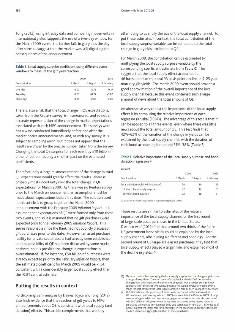
136 Quarterly Bulletin 2012 Q2
Tong (2012), using intraday data and comparing movements ininternational yields, supports the use of a two-day window forthe March 2009 event; the further falls in gilt yields the dayafter seem to suggest that the market was still digesting theconsequences of the announcement.
There is also a risk that the total change in QE expectations,taken from the Reuters survey, is mismeasured, and so not anaccurate representation of the change in market expectationsassociated with each MPC announcement. The surveys werenot always conducted immediately before and after themarket notice announcements, and, as with any survey, it issubject to sampling error. But it does not appear that theresults are driven by the precise number taken from the survey.Changing the total QE surprise for each event by £10 billion ineither direction has only a small impact on the estimatedcoefficients.
Therefore, only a large mismeasurement of the change in totalQE expectations would greatly affect the results. There isprobably most uncertainty over the total change in QEexpectations for March 2009. As there was no Reuters surveyprior to the March announcement, an assumption must bemade about expectations before this date. The solution usedin this article is to group together the March 2009announcement with the February 2009 Inflation Report. It isassumed that expectations of QE were formed only from thesetwo events, and so it is assumed that no gilt purchases wereexpected prior to the February 2009 Inflation Report. Thisseems reasonable since the Bank had not publicly discussedgilt purchases prior to this date. However, an asset purchasefacility for private sector assets had already been establishedand the possibility of QE had been discussed by some marketanalysts; so it is possible the change in expectations isoverestimated. If, for instance, £50 billion of purchases werealready expected prior to the February Inflation Report, thenthe estimated coefficient for March 2009 would be -1.24;consistent with a considerably larger local supply effect thanthe -0.81 central estimate.
Putting the results in context
Forthcoming Bank analysis by Daines, Joyce and Tong (2012)also finds evidence that the reaction of gilt yields to MPCannouncements about QE is consistent with local supply (andduration) effects. This article complements that work by
attempting to quantify the size of the local supply channel. Toput these estimates in context, the total contribution of thelocal supply surprise variable can be compared to the totalchange in gilt yields attributed to QE.
For March 2009, the contribution can be estimated bymultiplying the local supply surprise variable by thecorresponding coefficient estimate from Table C. Thissuggests that the local supply effect accounted for46 basis points of the total 93 basis point decline in 5–25 yearmaturity gilt yields. The March 2009 event should provide agood approximation of the overall importance of the localsupply channel because this event contained such a largeamount of news about the total amount of QE.(1)
An alternative way to test the importance of the local supplyeffect is by computing the relative importance of eachregressor (Kruskal (1987)). The advantage of this test is that itcan be applied to all three events, even where there was littlenews about the total amount of QE. This test finds that42%–62% of the variation of the change in yields can beexplained by the local supply channel, with the duration ofeach bond accounting for around 31%–38% (Table F).
These results are similar to estimates of the relativeimportance of the local supply channel for the first round of large-scale asset purchases in the United States. D’Amico et al (2012) find that around two thirds of the fall inUS government bond yields could be explained by the localsupply channel, albeit using a different methodology. For thesecond round of US large-scale asset purchases, they find thatlocal supply effects played a larger role, and explained most ofthe decline in yields.(2)
(1) This exercise involves averaging the local supply surprise and the change in yields overa range of maturities. The exercise is informative for March 2009 because thechanges over this range are all in the same direction. But a similar exercise is notappropriate for the other two events, because this would involve averaging over arange for part of which the local supply surprise is zero or even in opposite directions.
(2) US$300 billion of US government bonds were purchased in the first round ofUS purchases, commencing in March 2009 and completed in October 2009. A largeamount of agency debt and agency mortgage-backed securities was also purchased.US$600 billion of US government bonds were purchased in the second round ofpurchases, announced in November 2010 and completed in June 2011. D’Amico et al(2012) suggest the larger role for local supply in the second round reflects the moremodest impact on aggregate duration of these purchases.
Table F Relative importance of the local supply surprise and bondduration regressors(a)
Per cent
2009 2012
Event window 5 March 6 August 9 February
Total variation explained (R-squared) 94 80 92
of which, local supply surprise 62 42 61
of which, bond duration 32 38 31
(a) Based on the relative importance of regressor test (Kruskal (1987)).
Table E Local supply surprise coefficient using different eventwindows to measure the gilt yield reaction
2009 2012
Event window 5 March 6 August 9 February
One-day 0.02 -0.76 -0.37
Two-day -0.81 -0.74 -0.80
Three-day -0.85 -0.86 -0.82
Research and analysis The impact of QE on gilt yields 137
The above analysis suggests that the local supply channel is animportant mechanism which may explain around half of theimpact of QE on gilt yields. Therefore the natural experimentsapproach is useful for identifying a considerable portion of theeffect of QE, and so some weight can be attached to theresults which suggest that the strength of this channel has notchanged since 2009.
The other channels from QE to gilt yields have not beenseparately identified, so it is not possible to draw conclusionsabout how they may have changed. Furthermore, the impacton gilt yields is only the first leg of the transmission tospending and inflation. Therefore, even though the strength ofthe local supply channel does not appear to have changed, theanalysis in this article cannot necessarily be used to drawconclusions about the wider economic effects of QE.
Conclusion
Estimating the impact of QE on gilt yields has becomeincreasingly difficult as MPC announcements about theamount of assets the Bank intends to purchase are now widely
anticipated by financial market participants, based oneconomic news and data releases. To overcome this problem,this article uses a novel way of identifying part of the impact ofQE on gilt yields, using natural experiments associated withchanges in the auction maturity sectors used for giltpurchases.
The reaction of gilt yields to these market notices closelymatches the news they contained about the way in whichfuture purchases were expected to be distributed across giltsof different maturities. This is consistent with an importantrole for the local supply channel. The regression estimates inthis article suggest this channel can account for around half ofthe reduction in gilt yields due to QE, so the approach used inthis article is useful for identifying a considerable portion ofthe impact of QE on gilt yields.
The estimated strength of the local supply channel is broadlysimilar across the three market notice events. These eventsspan the period of QE purchases, so the strength of thisparticular channel does not appear to have changedsignificantly since QE was introduced in early 2009.
References
D’Amico, S, English, W, López-Salido, D and Nelson, E (2012), ‘TheFederal Reserve’s large-scale asset purchase programs: rationale andeffects’, Federal Reserve Board Working Paper, forthcoming.
Daines, M, Joyce, M and Tong, M (2012), ‘QE and the gilt market: adisaggregated analysis’, Bank of England Working Paper, forthcoming.
Fisher, P (2010), ‘An unconventional journey: The Bank of England’sasset purchase programme’, available atwww.bankofengland.co.uk/publications/Documents/speeches/2010/speech453.pdf.
Joyce, M, Lasaosa, A, Stevens, I and Tong, M (2011), ‘The financialmarket impact of quantitative easing in the United Kingdom’,International Journal of Central Banking, Vol. 7, No. 3, pages 113–61.
Joyce, M, Tong, M and Woods, R (2011), ‘The United Kingdom’squantitative easing policy: design, operation and impact’, Bank ofEngland Quarterly Bulletin, Vol. 51, No. 3, pages 200–12.
Kruskal, W (1987), ‘Relative importance by averaging over orderings’,The American Statistician, Vol. 41, No. 1, pages 6–10.
Vayanos, D and Vila, J-L (2009), ‘A preferred-habitat model of theterm structure of interest rates’, NBER Working Paper No. 15487.
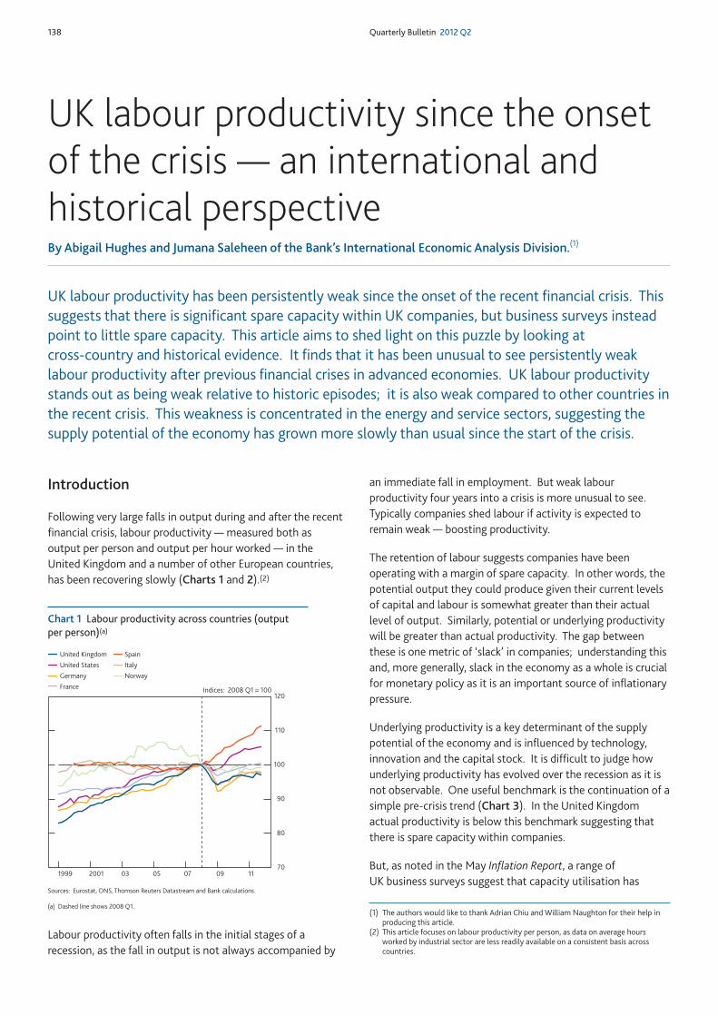
138 Quarterly Bulletin 2012 Q2
Introduction
Following very large falls in output during and after the recentfinancial crisis, labour productivity — measured both asoutput per person and output per hour worked — in theUnited Kingdom and a number of other European countries,has been recovering slowly (Charts 1 and 2).(2)
Labour productivity often falls in the initial stages of arecession, as the fall in output is not always accompanied by
an immediate fall in employment. But weak labourproductivity four years into a crisis is more unusual to see.Typically companies shed labour if activity is expected toremain weak — boosting productivity.
The retention of labour suggests companies have beenoperating with a margin of spare capacity. In other words, thepotential output they could produce given their current levelsof capital and labour is somewhat greater than their actuallevel of output. Similarly, potential or underlying productivitywill be greater than actual productivity. The gap betweenthese is one metric of ‘slack’ in companies; understanding thisand, more generally, slack in the economy as a whole is crucialfor monetary policy as it is an important source of inflationarypressure.
Underlying productivity is a key determinant of the supplypotential of the economy and is influenced by technology,innovation and the capital stock. It is difficult to judge howunderlying productivity has evolved over the recession as it isnot observable. One useful benchmark is the continuation of asimple pre-crisis trend (Chart 3). In the United Kingdomactual productivity is below this benchmark suggesting thatthere is spare capacity within companies.
But, as noted in the May Inflation Report, a range ofUK business surveys suggest that capacity utilisation has
UK labour productivity has been persistently weak since the onset of the recent financial crisis. Thissuggests that there is significant spare capacity within UK companies, but business surveys insteadpoint to little spare capacity. This article aims to shed light on this puzzle by looking atcross-country and historical evidence. It finds that it has been unusual to see persistently weaklabour productivity after previous financial crises in advanced economies. UK labour productivitystands out as being weak relative to historic episodes; it is also weak compared to other countries inthe recent crisis. This weakness is concentrated in the energy and service sectors, suggesting thesupply potential of the economy has grown more slowly than usual since the start of the crisis.
UK labour productivity since the onsetof the crisis — an international andhistorical perspectiveBy Abigail Hughes and Jumana Saleheen of the Bank’s International Economic Analysis Division.(1)
(1) The authors would like to thank Adrian Chiu and William Naughton for their help inproducing this article.
(2) This article focuses on labour productivity per person, as data on average hoursworked by industrial sector are less readily available on a consistent basis acrosscountries.
Chart 1 Labour productivity across countries (outputper person)(a)
70
80
90
100
110
120
1999 2001 03 05 07 09 11
Norway
United States
Spain
Germany
Italy
United Kingdom
FranceIndices: 2008 Q1 = 100
Sources: Eurostat, ONS, Thomson Reuters Datastream and Bank calculations.
(a) Dashed line shows 2008 Q1.
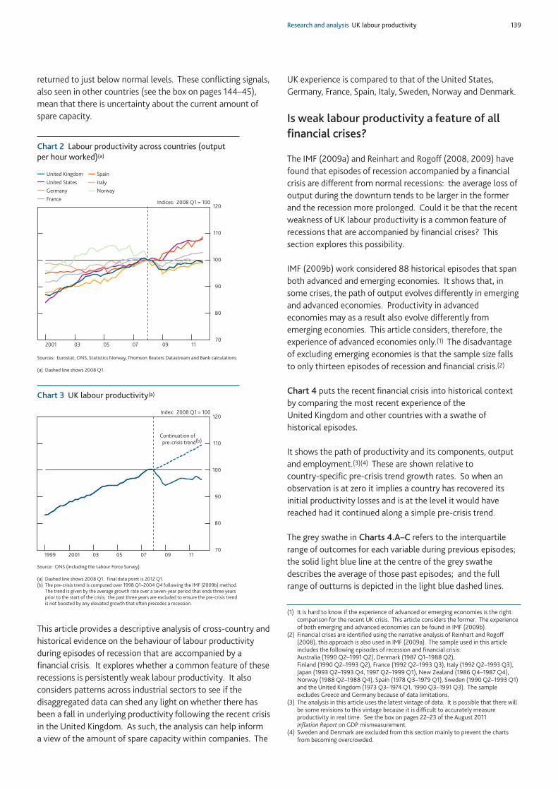
Research and analysis UK labour productivity 139
returned to just below normal levels. These conflicting signals,also seen in other countries (see the box on pages 144–45),mean that there is uncertainty about the current amount ofspare capacity.
This article provides a descriptive analysis of cross-country andhistorical evidence on the behaviour of labour productivityduring episodes of recession that are accompanied by afinancial crisis. It explores whether a common feature of theserecessions is persistently weak labour productivity. It alsoconsiders patterns across industrial sectors to see if thedisaggregated data can shed any light on whether there hasbeen a fall in underlying productivity following the recent crisisin the United Kingdom. As such, the analysis can help informa view of the amount of spare capacity within companies. The
UK experience is compared to that of the United States,Germany, France, Spain, Italy, Sweden, Norway and Denmark.
Is weak labour productivity a feature of allfinancial crises?
The IMF (2009a) and Reinhart and Rogoff (2008, 2009) havefound that episodes of recession accompanied by a financialcrisis are different from normal recessions: the average loss ofoutput during the downturn tends to be larger in the formerand the recession more prolonged. Could it be that the recentweakness of UK labour productivity is a common feature ofrecessions that are accompanied by financial crises? Thissection explores this possibility.
IMF (2009b) work considered 88 historical episodes that spanboth advanced and emerging economies. It shows that, insome crises, the path of output evolves differently in emergingand advanced economies. Productivity in advancedeconomies may as a result also evolve differently fromemerging economies. This article considers, therefore, theexperience of advanced economies only.(1) The disadvantageof excluding emerging economies is that the sample size fallsto only thirteen episodes of recession and financial crisis.(2)
Chart 4 puts the recent financial crisis into historical contextby comparing the most recent experience of theUnited Kingdom and other countries with a swathe ofhistorical episodes.
It shows the path of productivity and its components, outputand employment.(3)(4) These are shown relative tocountry-specific pre-crisis trend growth rates. So when anobservation is at zero it implies a country has recovered itsinitial productivity losses and is at the level it would havereached had it continued along a simple pre-crisis trend.
The grey swathe in Charts 4.A–C refers to the interquartilerange of outcomes for each variable during previous episodes;the solid light blue line at the centre of the grey swathedescribes the average of those past episodes; and the fullrange of outturns is depicted in the light blue dashed lines.
Chart 2 Labour productivity across countries (outputper hour worked)(a)
70
80
90
100
110
120
2001 03 05 07 09 11
Indices: 2008 Q1 = 100
Norway
United States
Spain
Germany
Italy
United Kingdom
France
Sources: Eurostat, ONS, Statistics Norway, Thomson Reuters Datastream and Bank calculations.
(a) Dashed line shows 2008 Q1.
Chart 3 UK labour productivity(a)
70
80
90
100
110
120
1999 2001 03 05 07 09 11
Index: 2008 Q1 = 100
Continuation of
pre-crisis trend(b)
Source: ONS (including the Labour Force Survey).
(a) Dashed line shows 2008 Q1. Final data point is 2012 Q1.(b) The pre-crisis trend is computed over 1998 Q1–2004 Q4 following the IMF (2009b) method.
The trend is given by the average growth rate over a seven-year period that ends three yearsprior to the start of the crisis; the past three years are excluded to ensure the pre-crisis trendis not boosted by any elevated growth that often precedes a recession.
(1) It is hard to know if the experience of advanced or emerging economies is the rightcomparison for the recent UK crisis. This article considers the former. The experienceof both emerging and advanced economies can be found in IMF (2009b).
(2) Financial crises are identified using the narrative analysis of Reinhart and Rogoff(2008), this approach is also used in IMF (2009a). The sample used in this articleincludes the following episodes of recession and financial crisis:Australia (1990 Q2–1991 Q2), Denmark (1987 Q1–1988 Q2),Finland (1990 Q2–1993 Q2), France (1992 Q2–1993 Q3), Italy (1992 Q2–1993 Q3),Japan (1993 Q2–1993 Q4, 1997 Q2–1999 Q1), New Zealand (1986 Q4–1987 Q4),Norway (1988 Q2–1988 Q4), Spain (1978 Q3–1979 Q1), Sweden (1990 Q2–1993 Q1)and the United Kingdom (1973 Q3–1974 Q1, 1990 Q3–1991 Q3). The sampleexcludes Greece and Germany because of data limitations.
(3) The analysis in this article uses the latest vintage of data. It is possible that there willbe some revisions to this vintage because it is difficult to accurately measureproductivity in real time. See the box on pages 22–23 of the August 2011Inflation Report on GDP mismeasurement.
(4) Sweden and Denmark are excluded from this section mainly to prevent the chartsfrom becoming overcrowded.
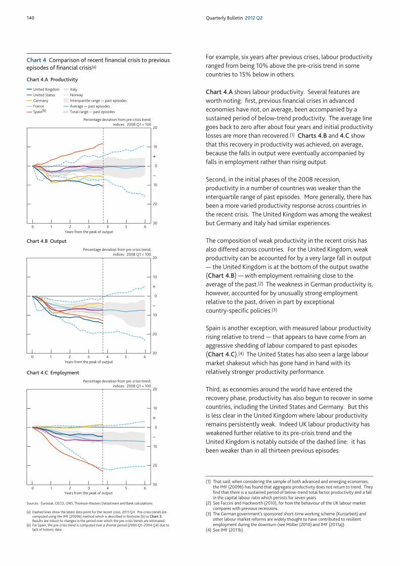
140 Quarterly Bulletin 2012 Q2
For example, six years after previous crises, labour productivityranged from being 10% above the pre-crisis trend in somecountries to 15% below in others.
Chart 4.A shows labour productivity. Several features areworth noting: first, previous financial crises in advancedeconomies have not, on average, been accompanied by asustained period of below-trend productivity. The average linegoes back to zero after about four years and initial productivitylosses are more than recovered.(1) Charts 4.B and 4.C showthat this recovery in productivity was achieved, on average,because the falls in output were eventually accompanied byfalls in employment rather than rising output.
Second, in the initial phases of the 2008 recession,productivity in a number of countries was weaker than theinterquartile range of past episodes. More generally, there hasbeen a more varied productivity response across countries inthe recent crisis. The United Kingdom was among the weakestbut Germany and Italy had similar experiences.
The composition of weak productivity in the recent crisis hasalso differed across countries. For the United Kingdom, weakproductivity can be accounted for by a very large fall in output— the United Kingdom is at the bottom of the output swathe(Chart 4.B) — with employment remaining close to theaverage of the past.(2) The weakness in German productivity is,however, accounted for by unusually strong employmentrelative to the past, driven in part by exceptionalcountry-specific policies.(3)
Spain is another exception, with measured labour productivityrising relative to trend — that appears to have come from anaggressive shedding of labour compared to past episodes(Chart 4.C).(4) The United States has also seen a large labourmarket shakeout which has gone hand in hand with itsrelatively stronger productivity performance.
Third, as economies around the world have entered therecovery phase, productivity has also begun to recover in somecountries, including the United States and Germany. But thisis less clear in the United Kingdom where labour productivityremains persistently weak. Indeed UK labour productivity hasweakened further relative to its pre-crisis trend and theUnited Kingdom is notably outside of the dashed line: it hasbeen weaker than in all thirteen previous episodes.
(1) That said, when considering the sample of both advanced and emerging economies,the IMF (2009b) has found that aggregate productivity does not return to trend. Theyfind that there is a sustained period of below-trend total factor productivity and a fallin the capital labour ratio which persists for seven years.
(2) See Faccini and Hackworth (2010), for how the behaviour of the UK labour marketcompares with previous recessions.
(3) The German government’s sponsored short-time working scheme (Kurzarbeit) andother labour market reforms are widely thought to have contributed to resilientemployment during the downturn (see Möller (2010) and IMF (2011a)).
(4) See IMF (2011b).
30
20
10
0
10
20
0 1 2 3 4 5 6
Interquartile range — past episodes
Total range — past episodes
Average — past episodes
Percentage deviation from pre-crisis trend;
indices: 2008 Q1 = 100
+
–
NorwayUnited States
Spain(b)
Germany
France
United Kingdom Italy
Years from the peak of output
Chart 4 Comparison of recent financial crisis to previousepisodes of financial crisis(a)
Chart 4.A Productivity
30
20
10
0
10
20
0 1 2 3 4 5 6
+
–
Percentage deviation from pre-crisis trend;
indices: 2008 Q1 = 100
Years from the peak of output
Chart 4.B Output
30
20
10
0
10
20
0 1 2 3 4 5 6
+
–
Percentage deviation from pre-crisis trend;
indices: 2008 Q1 = 100
Years from the peak of output
Sources: Eurostat, OECD, ONS, Thomson Reuters Datastream and Bank calculations.
(a) Dashed lines show the latest data point for the recent crisis, 2011 Q4. Pre-crisis trends arecomputed using the IMF (2009b) method which is described in footnote (b) to Chart 3.Results are robust to changes in the period over which the pre-crisis trends are estimated.
(b) For Spain, the pre-crisis trend is computed over a shorter period (2000 Q1–2004 Q4) due tolack of historic data.
Chart 4.C Employment
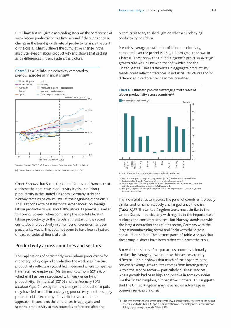
Research and analysis UK labour productivity 141
But Chart 4.A will give a misleading steer on the persistence ofweak labour productivity this time around if there has been achange in the trend growth rate of productivity since the startof the crisis. Chart 5 shows the cumulative change in theabsolute level of labour productivity and shows that settingaside differences in trends alters the picture.
Chart 5 shows that Spain, the United States and France are ator above their pre-crisis productivity levels. But labourproductivity in the United Kingdom, Germany, Italy andNorway remains below its level at the beginning of the crisis.This is at odds with past historical experiences: on averagelabour productivity was about 10% above its pre-crisis level atthis point. So even when comparing the absolute level oflabour productivity to their levels at the start of the recentcrisis, labour productivity in a number of countries has beenpersistently weak. This does not seem to have been a featureof past episodes of financial crisis.
Productivity across countries and sectors
The implications of persistently weak labour productivity formonetary policy depend on whether the weakness in actualproductivity reflects a cyclical fall in demand where companieshave retained employees (Martin and Rowthorn (2012)), orwhether it has been associated with weak underlyingproductivity. Benito et al (2010) and the February 2012Inflation Report investigate how changes to production inputsmay have led to a fall in underlying productivity and the supplypotential of the economy. This article uses a differentapproach; it considers the differences in aggregate andsectoral productivity across countries before and after the
recent crisis to try to shed light on whether underlyingproductivity has fallen.
Pre-crisis average growth rates of labour productivity,computed over the period 1998 Q1–2004 Q4, are shown inChart 6. These show the United Kingdom’s pre-crisis averagegrowth rate was in line with that of Sweden and theUnited States. These differences in aggregate productivitytrends could reflect differences in industrial structures and/ordifferences in sectoral trends across countries.
The industrial structure across the panel of countries is broadlysimilar and remains relatively unchanged since the crisis(Table A).(1) The United Kingdom looks most similar to theUnited States — particularly with regards to the importance ofbusiness and consumer services. But Norway stands out withthe largest extraction and utilities sector, Germany with thelargest manufacturing sector and Spain with the largestconstruction sector. The bottom panel of Table A shows thatthese output shares have been rather stable over the crisis.
But while the shares of output across countries is broadlysimilar, the average growth rates within sectors are verydifferent. Table B shows that much of the disparity in thepre-crisis average growth rates comes from heterogeneitywithin the service sector — particularly business services,where growth had been high and positive in some countrieslike the United Kingdom, but negative in others. This suggeststhat the United Kingdom may have had an advantage inbusiness services pre-crisis.
80
90
100
110
120
130
0 1 2 3 4 5 6
Indices: 2008 Q1 = 100
Interquartile range — past episodes
Total range — past episodes
Average — past episodes
NorwayUnited States
Spain
Germany
France
United Kingdom Italy
Years from the peak of output
Sources: Eurostat, OECD, ONS, Thomson Reuters Datastream and Bank calculations.
(a) Dashed lines show latest available data point for the recent crisis, 2011 Q4.
Chart 5 Level of labour productivity compared toprevious episodes of financial crisis(a)
0.5
0.0
0.5
1.0
1.5
2.0
2.5
3.0
Un
ited
Kin
gdo
m
Un
ited
Sta
tes(b
)
Ger
man
y
Fran
ce
Ital
y
Sp
ain
(c)
Sw
eden
No
rway
Den
mar
k
Pre-crisis (1998 Q1–2004 Q4)Per cent
+
–
Sources: Bureau of Economic Analysis, Eurostat and Bank calculations.
(a) Pre-crisis averages are computed using the IMF (2009b) method which is described infootnote (b) to Chart 3. Results are robust to choice of sample period.
(b) US average is computed using annual data from 1998–2004 to ensure trends are comparablewith the sectoral breakdown reported in Tables A and B.
(c) For Spain, the pre-crisis average is computed over a shorter period (2001 Q1–2004 Q4) dueto lack of historic data.
Chart 6 Estimated pre-crisis average growth rates oflabour productivity across countries(a)
(1) The employment shares across industry follow a broadly similar pattern to the outputshares reported in Table A. Spain is an exception where employment in constructionfell by 4 percentage points to 9% in 2010.
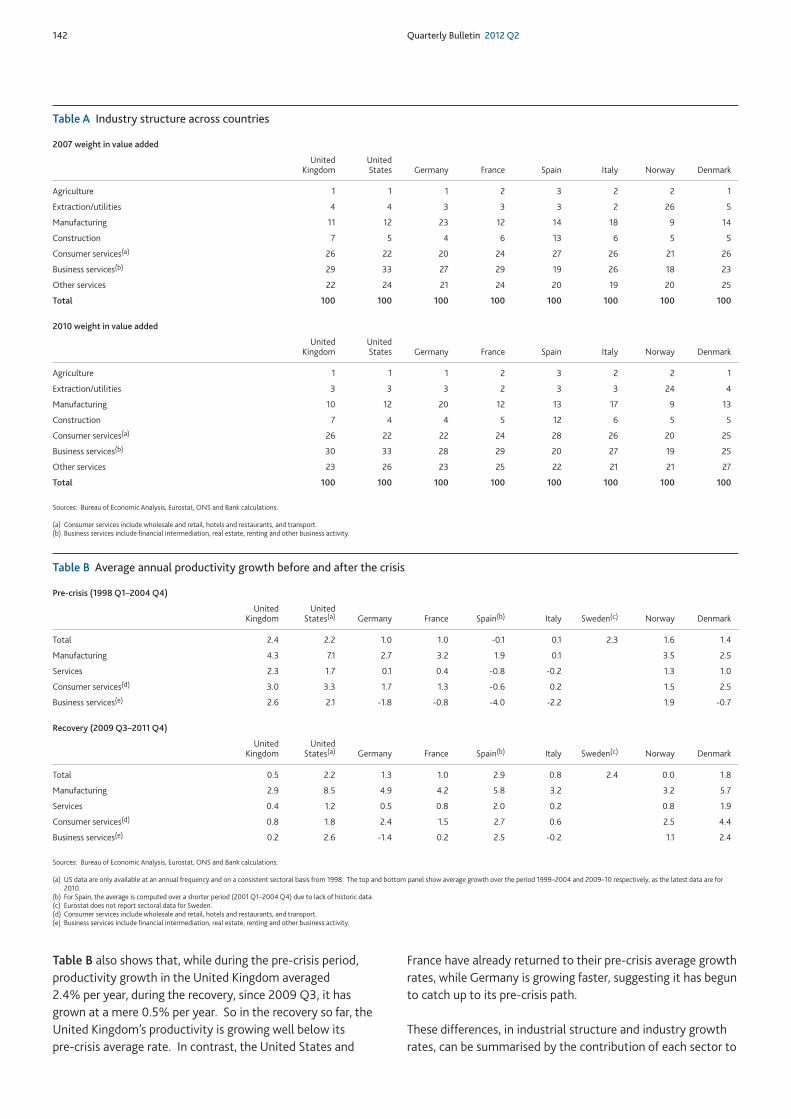
142 Quarterly Bulletin 2012 Q2
Table B also shows that, while during the pre-crisis period,productivity growth in the United Kingdom averaged2.4% per year, during the recovery, since 2009 Q3, it hasgrown at a mere 0.5% per year. So in the recovery so far, theUnited Kingdom’s productivity is growing well below itspre-crisis average rate. In contrast, the United States and
France have already returned to their pre-crisis average growthrates, while Germany is growing faster, suggesting it has begunto catch up to its pre-crisis path.
These differences, in industrial structure and industry growthrates, can be summarised by the contribution of each sector to
Table B Average annual productivity growth before and after the crisis
Pre-crisis (1998 Q1–2004 Q4)
United UnitedKingdom States(a) Germany France Spain(b) Italy Sweden(c) Norway Denmark
Total 2.4 2.2 1.0 1.0 -0.1 0.1 2.3 1.6 1.4
Manufacturing 4.3 7.1 2.7 3.2 1.9 0.1 3.5 2.5
Services 2.3 1.7 0.1 0.4 -0.8 -0.2 1.3 1.0
Consumer services(d) 3.0 3.3 1.7 1.3 -0.6 0.2 1.5 2.5
Business services(e) 2.6 2.1 -1.8 -0.8 -4.0 -2.2 1.9 -0.7
Recovery (2009 Q3–2011 Q4)
United UnitedKingdom States(a) Germany France Spain(b) Italy Sweden(c) Norway Denmark
Total 0.5 2.2 1.3 1.0 2.9 0.8 2.4 0.0 1.8
Manufacturing 2.9 8.5 4.9 4.2 5.8 3.2 3.2 5.7
Services 0.4 1.2 0.5 0.8 2.0 0.2 0.8 1.9
Consumer services(d) 0.8 1.8 2.4 1.5 2.7 0.6 2.5 4.4
Business services(e) 0.2 2.6 -1.4 0.2 2.5 -0.2 1.1 2.4
Sources: Bureau of Economic Analysis, Eurostat, ONS and Bank calculations.
(a) US data are only available at an annual frequency and on a consistent sectoral basis from 1998. The top and bottom panel show average growth over the period 1999–2004 and 2009–10 respectively, as the latest data are for2010.
(b) For Spain, the average is computed over a shorter period (2001 Q1–2004 Q4) due to lack of historic data.(c) Eurostat does not report sectoral data for Sweden.(d) Consumer services include wholesale and retail, hotels and restaurants, and transport.(e) Business services include financial intermediation, real estate, renting and other business activity.
Table A Industry structure across countries
2007 weight in value added
United UnitedKingdom States Germany France Spain Italy Norway Denmark
Agriculture 1 1 1 2 3 2 2 1
Extraction/utilities 4 4 3 3 3 2 26 5
Manufacturing 11 12 23 12 14 18 9 14
Construction 7 5 4 6 13 6 5 5
Consumer services(a) 26 22 20 24 27 26 21 26
Business services(b) 29 33 27 29 19 26 18 23
Other services 22 24 21 24 20 19 20 25
Total 100 100 100 100 100 100 100 100
2010 weight in value added
United UnitedKingdom States Germany France Spain Italy Norway Denmark
Agriculture 1 1 1 2 3 2 2 1
Extraction/utilities 3 3 3 2 3 3 24 4
Manufacturing 10 12 20 12 13 17 9 13
Construction 7 4 4 5 12 6 5 5
Consumer services(a) 26 22 22 24 28 26 20 25
Business services(b) 30 33 28 29 20 27 19 25
Other services 23 26 23 25 22 21 21 27
Total 100 100 100 100 100 100 100 100
Sources: Bureau of Economic Analysis, Eurostat, ONS and Bank calculations.
(a) Consumer services include wholesale and retail, hotels and restaurants, and transport.(b) Business services include financial intermediation, real estate, renting and other business activity.
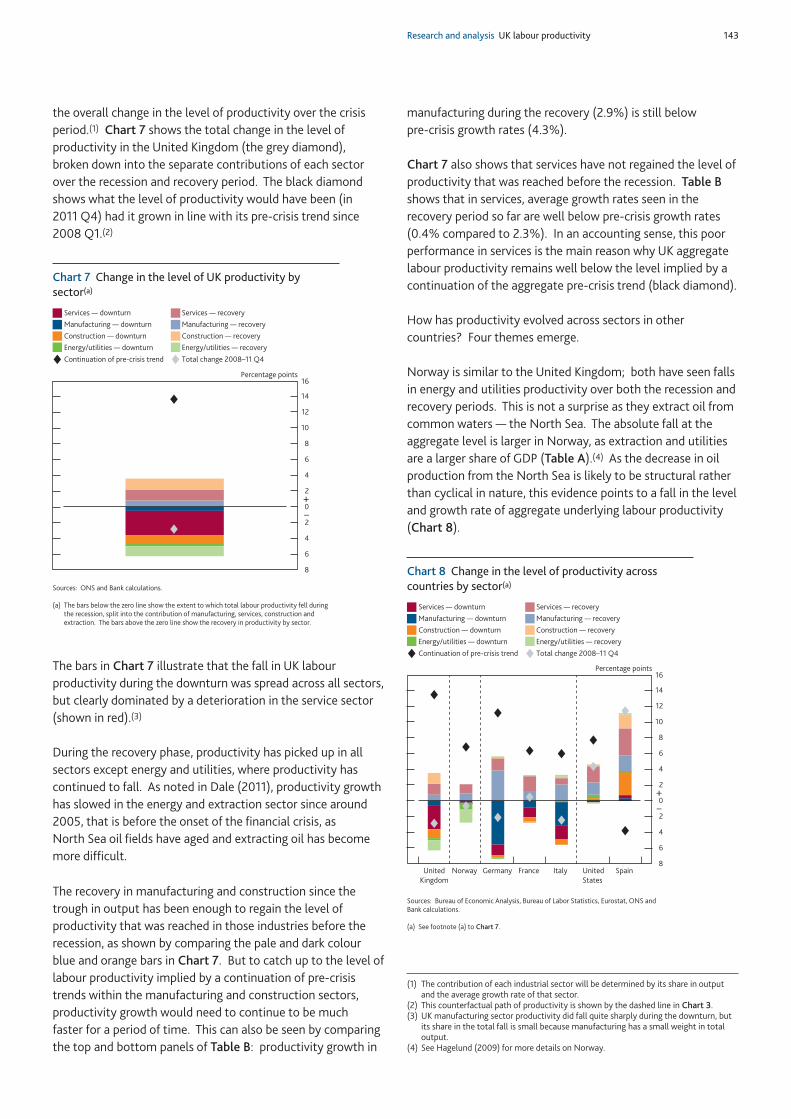
Research and analysis UK labour productivity 143
the overall change in the level of productivity over the crisisperiod.(1) Chart 7 shows the total change in the level ofproductivity in the United Kingdom (the grey diamond),broken down into the separate contributions of each sectorover the recession and recovery period. The black diamondshows what the level of productivity would have been (in2011 Q4) had it grown in line with its pre-crisis trend since2008 Q1.(2)
The bars in Chart 7 illustrate that the fall in UK labourproductivity during the downturn was spread across all sectors,but clearly dominated by a deterioration in the service sector(shown in red).(3)
During the recovery phase, productivity has picked up in allsectors except energy and utilities, where productivity hascontinued to fall. As noted in Dale (2011), productivity growthhas slowed in the energy and extraction sector since around2005, that is before the onset of the financial crisis, asNorth Sea oil fields have aged and extracting oil has becomemore difficult.
The recovery in manufacturing and construction since thetrough in output has been enough to regain the level ofproductivity that was reached in those industries before therecession, as shown by comparing the pale and dark colourblue and orange bars in Chart 7. But to catch up to the level oflabour productivity implied by a continuation of pre-crisistrends within the manufacturing and construction sectors,productivity growth would need to continue to be muchfaster for a period of time. This can also be seen by comparingthe top and bottom panels of Table B: productivity growth in
manufacturing during the recovery (2.9%) is still belowpre-crisis growth rates (4.3%).
Chart 7 also shows that services have not regained the level ofproductivity that was reached before the recession. Table Bshows that in services, average growth rates seen in therecovery period so far are well below pre-crisis growth rates(0.4% compared to 2.3%). In an accounting sense, this poorperformance in services is the main reason why UK aggregatelabour productivity remains well below the level implied by acontinuation of the aggregate pre-crisis trend (black diamond).
How has productivity evolved across sectors in othercountries? Four themes emerge.
Norway is similar to the United Kingdom; both have seen fallsin energy and utilities productivity over both the recession andrecovery periods. This is not a surprise as they extract oil fromcommon waters — the North Sea. The absolute fall at theaggregate level is larger in Norway, as extraction and utilitiesare a larger share of GDP (Table A).(4) As the decrease in oilproduction from the North Sea is likely to be structural ratherthan cyclical in nature, this evidence points to a fall in the leveland growth rate of aggregate underlying labour productivity(Chart 8).
8
6
4
2
0
2
4
6
8
10
12
14
Percentage points
+
–
Manufacturing — downturn
Services — downturn
Construction — downturn
Energy/utilities — downturn
Manufacturing — recovery
Services — recovery
Construction — recovery
Energy/utilities — recovery
Total change 2008–11 Q4Continuation of pre-crisis trend
16
Sources: ONS and Bank calculations.
(a) The bars below the zero line show the extent to which total labour productivity fell duringthe recession, split into the contribution of manufacturing, services, construction andextraction. The bars above the zero line show the recovery in productivity by sector.
Chart 7 Change in the level of UK productivity bysector(a)
UnitedKingdom
Norway Germany France Italy UnitedStates
Spain 8
6
4
2
0
2
4
6
8
10
12
14
Percentage points
+
–
Manufacturing — downturn
Services — downturn
Construction — downturn
Energy/utilities — downturn
Manufacturing — recovery
Services — recovery
Construction — recovery
Energy/utilities — recovery
Total change 2008–11 Q4Continuation of pre-crisis trend
16
Sources: Bureau of Economic Analysis, Bureau of Labor Statistics, Eurostat, ONS andBank calculations.
(a) See footnote (a) to Chart 7.
Chart 8 Change in the level of productivity acrosscountries by sector(a)
(1) The contribution of each industrial sector will be determined by its share in outputand the average growth rate of that sector.
(2) This counterfactual path of productivity is shown by the dashed line in Chart 3.(3) UK manufacturing sector productivity did fall quite sharply during the downturn, but
its share in the total fall is small because manufacturing has a small weight in totaloutput.
(4) See Hagelund (2009) for more details on Norway.
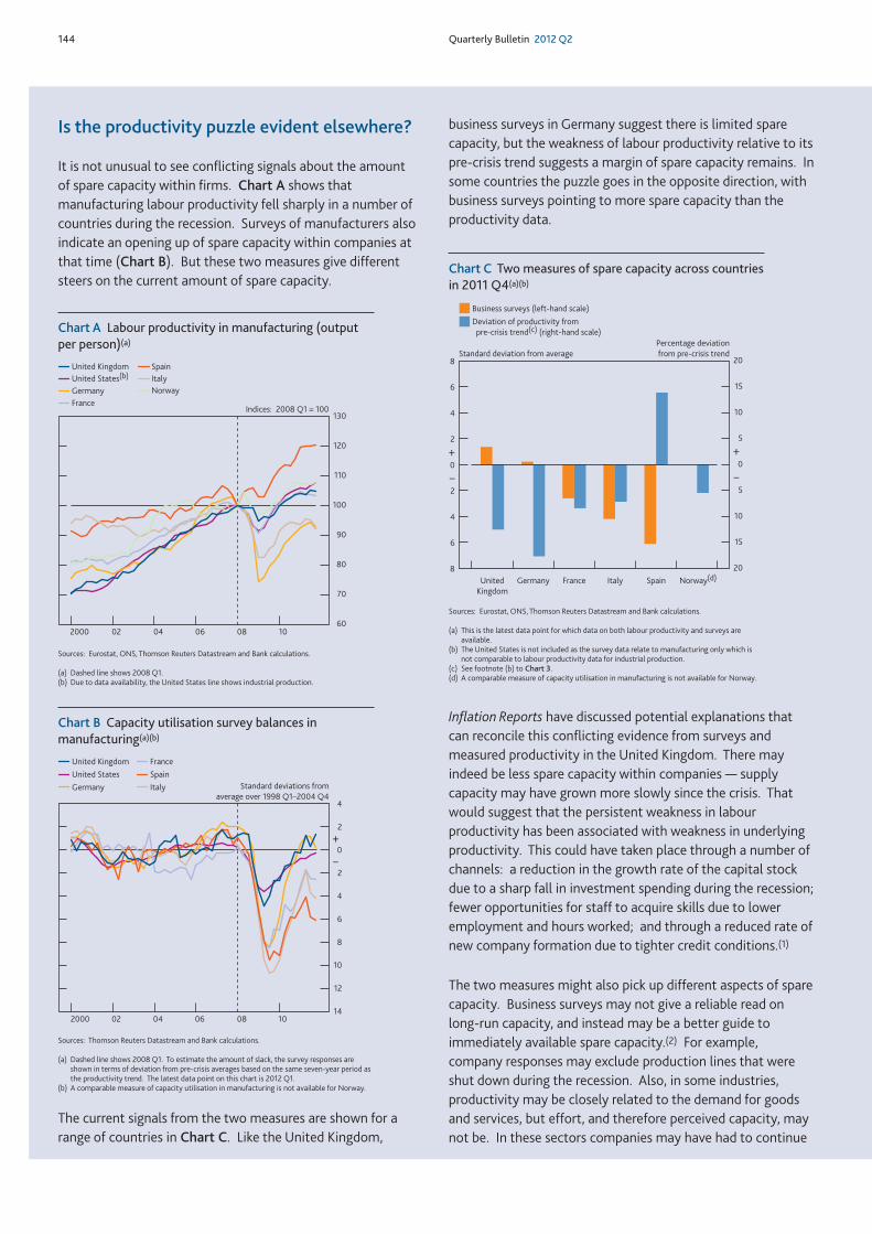
144 Quarterly Bulletin 2012 Q2
Is the productivity puzzle evident elsewhere?
It is not unusual to see conflicting signals about the amountof spare capacity within firms. Chart A shows thatmanufacturing labour productivity fell sharply in a number ofcountries during the recession. Surveys of manufacturers alsoindicate an opening up of spare capacity within companies atthat time (Chart B). But these two measures give differentsteers on the current amount of spare capacity.
The current signals from the two measures are shown for arange of countries in Chart C. Like the United Kingdom,
business surveys in Germany suggest there is limited sparecapacity, but the weakness of labour productivity relative to itspre-crisis trend suggests a margin of spare capacity remains. Insome countries the puzzle goes in the opposite direction, withbusiness surveys pointing to more spare capacity than theproductivity data.
Inflation Reports have discussed potential explanations thatcan reconcile this conflicting evidence from surveys andmeasured productivity in the United Kingdom. There mayindeed be less spare capacity within companies — supplycapacity may have grown more slowly since the crisis. Thatwould suggest that the persistent weakness in labourproductivity has been associated with weakness in underlyingproductivity. This could have taken place through a number ofchannels: a reduction in the growth rate of the capital stockdue to a sharp fall in investment spending during the recession;fewer opportunities for staff to acquire skills due to loweremployment and hours worked; and through a reduced rate ofnew company formation due to tighter credit conditions.(1)
The two measures might also pick up different aspects of sparecapacity. Business surveys may not give a reliable read onlong-run capacity, and instead may be a better guide toimmediately available spare capacity.(2) For example,company responses may exclude production lines that wereshut down during the recession. Also, in some industries,productivity may be closely related to the demand for goodsand services, but effort, and therefore perceived capacity, maynot be. In these sectors companies may have had to continue
14
12
8
6
4
2
0
2
4
2000 02 04 06 08 10
Standard deviations from
average over 1998 Q1–2004 Q4
10
+
–
FranceUnited Kingdom
Germany
Spain
Italy
United States
Sources: Thomson Reuters Datastream and Bank calculations.
(a) Dashed line shows 2008 Q1. To estimate the amount of slack, the survey responses areshown in terms of deviation from pre-crisis averages based on the same seven-year period asthe productivity trend. The latest data point on this chart is 2012 Q1.
(b) A comparable measure of capacity utilisation in manufacturing is not available for Norway.
Chart B Capacity utilisation survey balances inmanufacturing(a)(b)
60
70
80
90
100
110
120
130
2000 02 04 06 08 10
Indices: 2008 Q1 = 100
Norway
France
United Kingdom
Germany
Spain
ItalyUnited States(b)
Sources: Eurostat, ONS, Thomson Reuters Datastream and Bank calculations.
(a) Dashed line shows 2008 Q1.(b) Due to data availability, the United States line shows industrial production.
Chart A Labour productivity in manufacturing (outputper person)(a)
20
15
10
5
0
5
10
15
20
8
6
4
2
0
2
4
6
8
United
Kingdom
Germany France Italy Spain Norway(d)
Business surveys (left-hand scale)
Deviation of productivity from
pre-crisis trend(c) (right-hand scale)
Percentage deviation
from pre-crisis trendStandard deviation from average
+
–
+
–
Sources: Eurostat, ONS, Thomson Reuters Datastream and Bank calculations.
(a) This is the latest data point for which data on both labour productivity and surveys areavailable.
(b) The United States is not included as the survey data relate to manufacturing only which isnot comparable to labour productivity data for industrial production.
(c) See footnote (b) to Chart 3.(d) A comparable measure of capacity utilisation in manufacturing is not available for Norway.
Chart C Two measures of spare capacity across countriesin 2011 Q4(a)(b)
Research and analysis UK labour productivity 145
In contrast to the United Kingdom, the falls in productivity inGermany, France and Italy are concentrated in manufacturing.Over the recovery, manufacturing productivity has grownfaster in these countries than in the United Kingdom, whichexplains why they have started to reclaim some of their lostground.
In the service sector, before the crisis, average productivitygrowth rates in the United Kingdom were high, particularly inbusiness services. But growth has been weak during therecovery. It is difficult to explain this weakness as a cyclicalpattern: the fall in services output was greater here thanelsewhere, which might otherwise have suggested a strongerrecovery. It is possible that the financial nature of the crisishas reduced underlying labour productivity in business andfinancial services. But the challenge to this view is why suchweakness is not evident in the United States, where thefinancial crisis originated and where the business servicessector is just as big as it is in the United Kingdom.
In the United States and Spain, productivity has continued togrow since the onset of the crisis as companies have shedlabour at a faster rate than output has fallen. Thediametrically opposite behaviour of labour productivity in theUnited Kingdom and the United States is of particular interest.These two countries have a similar industrial structure, butcompanies in each have reacted very differently in the extentto which they have shed or retained labour.
Conclusion
The behaviour of labour productivity in the United Kingdomhas been puzzling: it has been persistently weak, suggestingthat as demand has remained weak there has been much morespare capacity in companies than implied by business surveys.
Persistently weak labour productivity is not a feature of pastepisodes of financial crisis, although it does seem to becommon across countries after the recent financial crisis.
Before the crisis, the United Kingdom had seen the fastestaverage rate of productivity growth in our sample. Thisperformance has worsened considerably since the crisis startedand average rates of productivity in the United Kingdom havebeen one of the slowest in our sample.
It is too early to say whether the level and growth rate ofUK labour productivity will remain weak, or whether, whendemand recovers, productivity will return to the higher ratesseen during the pre-crisis period. Cross-country, cross-sectoranalysis shows the weakness to be concentrated in the energyand service sectors. The energy sector trends are more likelyto be structural rather than cyclical and so point to a possiblefall in underlying productivity. While there is no hard evidencethat low productivity in the service sector is structural, the lowgrowth rates witnessed in the post-crisis period have been somuch weaker than the pre-crisis average rates for so long thatit is hard to ignore the possibility that underlying productivityin this sector may have slowed.
Overall, these findings are consistent with the Monetary PolicyCommittee’s judgement in the May 2011 Inflation Report(page 55) that underlying productivity growth is likely to havebeen weaker than usual since the start of the crisis, althoughthere is considerable uncertainty in any evaluation ofunderlying productivity growth. It is, however, likely that,alongside substantial spare capacity within the labour market,a margin of spare capacity remains within companies.
to work their factors of production, even as output has fallen.As an example, estate agents may be working intensively eventhough the volume of business has declined, because it hasbecome harder to match buyers and sellers in a thin market. Ifthis were the case, labour productivity could recover whendemand recovers, even though the survey responses indicatelittle spare capacity. Similarly, if companies have held on toemployees during the recession because they have felt it
would be too costly to fire and then rehire skilled staff whendemand recovers, productivity growth could rise quite sharplyif output growth picks up, although it might also pick up ifcompanies decide to let surplus staff go.
(1) For evidence on each of these channels see Disney, Haskel and Heden (2003), and theNovember 2011 and February 2012 Inflation Reports.
(2) Also, it is not straightforward to map the qualitative information that is collected inthe surveys into quantitative measures of spare capacity. See Cunningham (1997).

146 Quarterly Bulletin 2012 Q2
References
Benito, A, Neiss, K, Price, S and Rachel, Ł (2010), ‘The impact of thefinancial crisis on supply’, Bank of England Quarterly Bulletin, Vol. 50,No. 2, pages 104–14.
Cunningham, A (1997), ‘Quantifying survey data’, Bank of EnglandQuarterly Bulletin, August, pages 292–300.
Dale, S (2011), ‘Productivity and monetary policy’, available atwww.bankofengland.co.uk/publications/Documents/speeches/2011/speech519.pdf.
Disney, R, Haskel, J and Heden, Y (2003), ‘Restructuring andproductivity growth in UK manufacturing’, Economic Journal, Vol. 113,Issue 489, pages 666–94.
Faccini, R and Hackworth, C (2010), ‘Changes in output,employment and wages during recessions in the United Kingdom’,Bank of England Quarterly Bulletin, Vol. 50, No. 1, pages 43–50.
Hagelund, K (2009), ‘Productivity growth in Norway 1948–2008’,Norges Bank Report, 2/2009.
IMF (2009a), ‘From recession to recovery: how soon and howstrong?’, World Economic Outlook, April, Chapter 3, pages 103–38.
IMF (2009b), ‘What’s the damage? Medium term output dynamicsafter financial crises’, World Economic Outlook, October, Chapter 4,pages 121–51.
IMF (2011a), ‘Germany — Staff Report for the 2011 Article IVConsultation’, IMF Country Report No. 11/168, July.
IMF (2011b), ‘Spain — Staff Report for the 2011 Article IVConsultation’, IMF Country Report No. 11/215, July.
Martin, B and Rowthorn, R (2012), ‘Is the British economy supplyconstrained?’, Centre for Business Research, University of Cambridge.
Möller, J (2010), ‘Germany’s job miracle in the world recession —shock-absorbing institutions in the manufacturing sector’, AppliedEconomics Quarterly, Vol. 61, pages 9–28.
Reinhart, C and Rogoff, K (2008), ‘Is the 2007 US sub-primefinancial crisis so different? An international historical comparison’,American Economic Review, Vol. 98, No. 2, pages 339–44.
Reinhart, C and Rogoff, K (2009), This time is different: eightcenturies of financial folly, Princeton University Press.
Research and analysis Payments in a bank’s recovery or resolution 147
Introduction
A payment is the transfer of money from one individual orbusiness to another. Payments are crucial to the efficientfunctioning of the economy. They are essential for individualsto receive their salary and pay their bills, for businesses to buyand sell goods and services, and for the Government to receivetaxes and make welfare payments.
The systems that facilitate payments(3) are a key componentof the United Kingdom’s financial infrastructure, ensuring thatbank(4) customers’ payment instructions result in paymentsreaching the intended destination on time. They are thereforeimportant to maintaining financial stability and confidence inthe banking system. Payment schemes, such as Bacs andCheque & Credit Clearing Company (C&CCC), are responsiblefor system governance and rules for participation.
When banks are operating under normal financial conditions,payments flow seamlessly between participants in the bankingsystem. But when a bank is recovering from a period of stressit may need to take specific actions to retain access to thepayment schemes while it recovers (so that its customers cancontinue to make and receive payments). A recovering bankmay be able to take these actions itself. But when a bank fails,and is taken into ‘resolution’, it is the authorities(5) that willtake action to ensure the failed bank’s customers can continue,or resume, their payments activity with minimal disruption.
This is critical to support financial stability because if a failedbank’s customers were unable to receive their salaries and paytheir bills for a prolonged period of time, this could impact the wider economy and cause a loss in confidence in thebanking system. The Bank of England is the resolutionauthority(6) and as such leads and manages the resolutionprocess for such firms (see the box on page 151) includingaspects on payments.
Bank recovery and resolution methods used in the past haveresulted in little or no disruption to payments. But thelandscape for bank recovery and resolutions is evolving and itis important that in future these processes do not result inundue disruption to payments. Following the publication ofthe Financial Stability Board’s(7) (2011) ‘Key attributes ofeffective resolution regimes for financial institutions’, theauthorities will be thinking about developments to the United Kingdom’s resolution planning which could potentiallyimpact plans for payment operations in resolution scenarios.
The robustness of payments infrastructure, and the associated ability of payments to flowseamlessly, is an important contributor to financial stability. The United Kingdom’s paymentsinfrastructure has historically proved to be efficient and robust. But, in a situation where a bank is indifficulty or fails, the need to ensure that customers can continue to make and receive paymentsmay become challenging. This article draws together and discusses some of the issues in the waythat UK payments and payment schemes work in stressed scenarios. It highlights some possibleenhancements which could help to achieve minimal disruption to payment flows in the event that abank gets into difficulty or fails — a subject the authorities, payment schemes and banks have beenaddressing in recent months. It looks at elements of recovery and resolution planning from thespecific perspective of retail payments.(2)
Considering the continuity ofpayments for customers in a bank’srecovery or resolutionBy Emma Carter of the Bank’s Customer Banking Division.(1)
(1) The author would like to thank Andrew Forrest for his help in producing this article. (2) It is not intended to represent in any way a comprehensive analysis or assessment of
any other aspect of recovery and resolution plans or resolution planning. (3) Interbank payment systems are arrangements designed to facilitate or control the
transfer of money between financial institutions who participate in the arrangements.(4) This article refers to all credit institutions as banks. (5) In this article ‘authorities’ refers to one or more of HM Treasury, the Financial Services
Authority and the Bank of England.(6) See Davies and Dobler (2011).(7) The Financial Stability Board was established to co-ordinate internationally the work
of national authorities and international standard setters and to develop andpromote the implementation of effective regulatory, supervisory and other financial sector policies in the interest of financial stability.
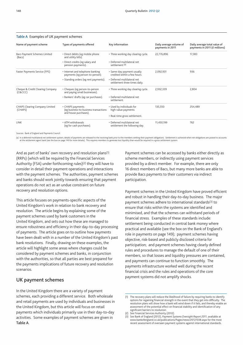
148 Quarterly Bulletin 2012 Q2
And as part of banks’ own recovery and resolution plans(1)
(RRPs) (which will be required by the Financial ServicesAuthority (FSA) under forthcoming rules)(2) they will have toconsider in detail their payment operations and interactionswith the payment schemes. The authorities, payment schemesand banks should work jointly towards ensuring that paymentoperations do not act as an undue constraint on futurerecovery and resolution options.
This article focuses on payments-specific aspects of the United Kingdom’s work in relation to bank recovery andresolution. The article begins by explaining some of thepayment schemes used by bank customers in the United Kingdom, and sets out how these are managed toensure robustness and efficiency in their day-to-day processingof payments. The article goes on to outline how paymentshave been dealt with in a number of the United Kingdom’s pastbank resolutions. Finally, drawing on these examples, thearticle will highlight some areas where changes could beconsidered by payment schemes and banks, in conjunctionwith the authorities, so that all parties are best prepared forthe payments implications of future recovery and resolutionscenarios.
UK payment schemes
In the United Kingdom there are a variety of paymentschemes, each providing a different service. Both wholesaleand retail payments are used by individuals and businesses inthe United Kingdom, but this article will focus on retailpayments which individuals primarily use in their day-to-dayactivities. Some examples of payment schemes are given inTable A.
Payment schemes can be accessed by banks either directly asscheme members, or indirectly using payment servicesprovided by a direct member. For example, there are only 16 direct members of Bacs, but many more banks are able toprovide Bacs payments to their customers via indirectparticipation.
Payment schemes in the United Kingdom have proved efficientand robust in handling their day-to-day business. The majorpayment schemes adhere to international standards(3) toensure that risks within the systems are identified andminimised, and that the schemes can withstand periods offinancial stress. Examples of these standards include:settlement being conducted in central bank money wherepractical and available (see the box on the Bank of England’srole in payments on page 149); payment schemes havingobjective, risk-based and publicly disclosed criteria forparticipation; and payment schemes having clearly definedrules and procedures to manage the default of one of theirmembers, so that losses and liquidity pressures are contained,and payments can continue to function smoothly. Thepayments infrastructure worked well during the recentfinancial crisis and the rules and operations of the corepayment systems did not amplify shocks.
(1) The recovery plans will reduce the likelihood of failure by requiring banks to identifyoptions for regaining financial strength in the event that they get into difficulty. Theresolution plans will show how a bank will wind down if it fails, and thereby enable anassessment of the potential effect on financial stability and identification of anysignificant barriers to resolution.
(2) See Financial Services Authority (2012). (3) See Bank of England (2012), Payment Systems Oversight Report 2011, available at
www.bankofengland.co.uk/publications/Pages/news/2012/038.aspx for the mostrecent assessment of overseen payment systems against international standards.
Table A Examples of UK payment schemes
Name of payment scheme Types of payments offered Key information Daily average volume of Daily average total value of payments in 2011 payments in 2011 (£ millions)
Bacs Payment Schemes Limited • Direct debits (eg mobile phone • Three working day clearing cycle. 22,776,896 17,383(Bacs) and utility bills).
• Direct credits (eg salary and • Deferred multilateral netpension payments). settlement.(a)
Faster Payments Service (FPS) • Internet and telephone banking • Same-day payment usually 2,092,931 936payments (eg person-to-person). credited within a few hours.
• Standing orders (eg rent payments). • Deferred multilateral netsettlement three times daily.
Cheque & Credit Clearing Company • Cheques (eg person-to-person • Three working day clearing cycle. 2,932,339 2,804(C&CCC) and paying small businesses).
• Bankers’ drafts (eg car purchases). • Deferred multilateral net settlement.
CHAPS Clearing Company Limited • CHAPS payments • Used by individuals for 135,550 254,489(CHAPS) (eg business-to-business transactions high-value payments.
and house purchases).• Real-time gross settlement.
LINK • ATM withdrawals • Deferred multilateral net 11,450,199 762(eg for cash purchases). settlement the following day.
Sources: Bank of England and Payments Council.
(a) In a deferred multilateral net settlement system, details of payments are released to the receiving bank prior to the members settling their payment obligations. Settlement is achieved when net obligations are posted to accountsat the settlement agent bank (see the box on page 149 for more details). This requires members to generate less liquidity than would be required in a gross settlement system.
Research and analysis Payments in a bank’s recovery or resolution 149
The United Kingdom’s existing payment schemes were notbuilt with bank recovery and resolution scenarios in mind.Therefore, schemes and banks may like to consider the impactthat these challenging scenarios may have on their operations.The ultimate goal is that disruption to payments is minimisedduring a bank’s recovery or resolution process, and thatpayments infrastructure and operations do not present barriersto the execution of any bank resolution method.
Considering retail payments in past bankresolutions
During a bank resolution, the ability of customers to continue,or resume, making and receiving payments is important tomaintaining financial stability (this includes retaining access totheir insured deposits).(1) The Bank has been involved in anumber of resolutions in recent years, both before and afterthe creation of the Special Resolution Regime (SRR) in 2009.
In all past resolutions the authorities have worked towardsthere being little or no disruption to the payment activities ofthe failed banks’ retail customers. One way that continuity ofpayments was achieved was by keeping the whole of a bankrunning as one entity. For example, in the case of Northern Rock, HM Treasury took the bank into temporarypublic ownership in February 2008. It remained solvent andcould continue to meet its payment obligations. It couldtherefore continue to provide banking services, including
payments, to its customers in exactly the same way as it didbefore. From a payments perspective, a resolution methodwhich keeps a bank together as one whole entity is the leastcomplicated option. This is still an option within the SRR. Forexample, by taking a whole bank into temporary publicownership, although this exposes public funds to the greatestrisk, and therefore the failure of a bank would need to pose aserious threat to financial stability in order for this option to beselected. Alternatively, a whole bank could be transferred to aprivate sector purchaser or to a bridge bank.(2)
In the case of Northern Rock, the bank was subsequently split in January 2010 into two entities: Northern Rock plc (a savings and mortgage bank) and Northern Rock (AssetManagement) plc (an asset management vehicle providing forthe orderly wind-down of the remaining business). Followingthis split, Northern Rock plc was able to continue to providepayment services to its customers as it acquired the ‘old’Northern Rock’s payment scheme membership and indirectparticipation relationships via a statutory Transfer Order,(3)
which stated the terms for separation. One of the payment
(1) For more information on the Financial Services Compensation Scheme insurancecoverage, see www.fscs.org.uk/what-we-cover/about-us/.
(2) A bridge bank is a subsidiary company set up by the Bank of England specifically tofacilitate a transfer of property, rights and obligations under the UK SpecialResolution Regime. It is wholly owned by the Bank of England, and authorised by theFSA to perform whatever regulated activities are required of it (such as takingdeposits).
(3) ‘The Northern Rock plc Transfer Order 2009’, available atwww.legislation.gov.uk/uksi/2009/3226/contents/made.
The Bank of England’s role in payments
The Bank has a variety of roles in relation to payments largelystemming from its objective to support financial stability:
• The Bank acts as settlement agent for members of CHAPS,Bacs, Faster Payments, LINK(1) and C&CCC. This means thatit provides accounts to payment scheme members to enablethem to settle their payment obligations between oneanother. These accounts are held in the Bank’s real-timegross settlement system (which provides for the immediatesettlement of payments with finality). Settling using moneyheld at the central bank is less risky than settling usingmoney held at a commercial bank as central bank money isthe ultimate risk-free settlement asset.
• The Bank oversees systemically important paymentsystems(2) under the statutory framework set out in Part 5 ofthe Banking Act 2009.(3) It assesses the risks that eachsystem could pose to financial stability and identifies areaswhere action should be taken to reduce risks (for furtherdetails see Bank of England (2012), Payment SystemsOversight Report 2011).
• The Bank requires payment scheme access itself in order toprovide banking services to its own customers (includingother central banks and UK Government departments), so itis also an operational user of some of the schemes.
• The Bank attends meetings of the Payments Council Board(the organisation which sets strategy for UK payments). Itparticipates in these meetings as an observer only and doesnot vote on decisions. It also has representation on theboards of relevant payment schemes.
• The Bank of England is the resolution authority for UK-incorporated firms authorised by the FSA to acceptdeposits. It decides which resolution tool to use andmanages its implementation.(4) The Bank and the FSA areworking together with individual banks on developing banks’recovery and resolution plans.
(1) Not all LINK members are able to hold a settlement account at the Bank as some arenot banks.
(2) Currently these are CHAPS, Bacs, Faster Payments and others outside the remit ofthis article (CLS, payments arrangements embedded in CREST, LCH.Clearnet and ICE Clear Europe).
(3) Banking Act 2009, Part 5, available at www.legislation.gov.uk/ukpga/2009/1/part/5. (4) With the exception of taking a bank into temporary public ownership which is the
decision of HM Treasury.
150 Quarterly Bulletin 2012 Q2
scheme memberships that it acquired was for Bacs, whichwould normally require an entity to have a minimum creditrating history in order to be eligible. As a new entity, Northern Rock plc did not have any credit rating history and sothe Transfer Order included a temporary waiver of Bacs’minimum credit rating membership criterion.
Another example of a successful resolution during whichdisruption for customers was closely managed was that ofSouthsea Mortgage and Investment Company Limited in June 2011. In this instance, the Bank Insolvency Procedure(BIP) was used since it was judged that the failure of the bankwould not have a systemic impact on the financial system.Southsea customers were paid their insured deposits (up to£85,000) automatically by the Financial ServicesCompensation Scheme (FSCS) via cheque soon after theresolution. They could then pay this into an alternative bankaccount, or open another account for this purpose. It wasappropriate to use the BIP tool in the case of Southsea as itwas a small bank which was not in the business of providingcurrent accounts, meaning that the remaining industry playerscould easily absorb its customers, and there was not a largenumber of people needing to contact their employers andservice providers to change their payment instructions.Disruption for Southsea’s customers was thus effectivelymanaged and the impact on the wider economy wascontained.
A resolution can become more complicated when the SRRtransfer tools are used to transfer part of a bank to a privatesector purchaser or bridge bank (see the box on page 151).When using the transfer tools to conduct a partial banktransfer it is still a priority to ensure the continuity ofpayments for customers. In the case of the DunfermlineBuilding Society resolution in March 2009, a private sectorpurchaser, Nationwide Building Society, acquired core parts ofthe business. A further portion was transferred to a small Bank of England bridge bank (this was later sold to Nationwidein July 2009) and the remainder of Dunfermline’s business wasplaced into the Building Society Special AdministrationProcedure. Nationwide acquired Dunfermline’s infrastructureand staff needed to run the business it had taken on, by virtueof the Bank’s property transfer instrument.(1) Nationwidecould then manage its newly acquired bank accounts usingDunfermline’s existing banking platform, meaning thatbanking services continued to operate normally for customers.Some payment services required by the bridge bank were alsoprovided by Nationwide so that customers of the bridge bankreceived continuity of service also.
Reflecting on use of the SRR
Although resolutions to date have been successfullyconducted with minimal impact on the continuity of customerpayments, these experiences can still be useful when
considering improvements and how to deal with morecomplicated scenarios in the future.
There are a number of variables which could increase thecomplexity and risk involved in the continuity of payments in afuture bank resolution. Some examples of these are:
• When using the transfer tools it may not always be possibleto find a sole private sector purchaser willing to buy themajority of the business. A bank may therefore need to besplit up into multiple parts for sale.
• A private sector purchaser may not always be a bank thathas existing access to the payment schemes (for example, itmay be an entity which did not previously provide a retailbanking business).
• A failing bank may be a direct member in the paymentschemes providing payment services to indirect participantbanks that are not scheme members themselves. Theseindirect participants may depend upon the failing bank tomake their customers’ payments and therefore there wouldalso be an impact on these indirect participant banks (andtheir customers) in the event of the direct member’s failure.
• It may not be possible to use the BIP tool on a large bank.Challenges to banking continuity may arise as there wouldbe more customers requiring FSCS payout and potentiallyrequiring new bank accounts to be opened. This could leadto capacity constraints on the FSCS and the remaining banksabsorbing the failed bank’s customers. The decision to usethe BIP tool would depend on the ability to pay out and forcustomers to resume their banking activities within areasonable amount of time.
Factors such as these may make a resolution more complex,and the provision of payments with minimal disruption moredifficult to achieve. It is therefore important that banks,payment schemes and authorities are well prepared for alleventualities in advance.
Preparing for future bank recovery andresolution scenarios
In 2011, the Bank led a Financial Stability Board (FSB)workstream looking at barriers to recovery and resolution inpayment operations. The Bank consulted with banks andpayment schemes in the United Kingdom in order tounderstand the issues from various perspectives. Discussionshighlighted some areas for further work and put forward somesuggestions for improvements in order to overcome existing
(1) A property transfer instrument is a legal instrument made by the Bank of Englandunder the Banking Act 2009, and has the legal effect of transferring property, rightsor liabilities of a failed bank to another entity.
Research and analysis Payments in a bank’s recovery or resolution 151
barriers to recovery and resolution stemming from payments.The group’s recommendations fed into the FSB report on ‘Key attributes of effective resolution regimes for financialinstitutions’.
The FSA’s future guidance and rules for RRPs will require banksto consider any payments issues that could hinder their abilityto recover or be resolved in an orderly manner. This work willinclude thinking about how they access the payment schemesand what they would be able to do to ensure that this access ismaintained without increasing risk for other payment schememembers, or any direct member providing them with paymentservices. It will also include, in a resolution context,
considering the potential need to split up their business lineswhile avoiding severe disruption to payments. This will beparticularly relevant for large banks which may have numerous business lines and legal entities sharing the samepayment scheme membership and pools of liquidity. Theremainder of this article sets out some of the issues and ideasthat were discussed during the workstream and relatedconsultations.
Retaining payment scheme membershipIt is helpful for payment schemes to understand how theirrules and processes may play out during the recovery orresolution of a member bank. For example, a minimum credit
The Special Resolution Regime objectives andtools
Following the financial crisis of 2008, the Banking Act 2009created the Special Resolution Regime (SRR) which gave theauthorities a permanent framework for dealing with distressedbanks. The SRR has a number of objectives:
• to protect and enhance the stability of the financial systemsof the United Kingdom;
• to protect and enhance public confidence in the stability ofthe banking systems of the United Kingdom;
• to protect depositors;• to protect public funds; and• to avoid interfering with property rights in contravention
of a Convention Right (within the meaning of the Human Rights Act 1998).(1)
Achieving the continuity of customer payments soon afterresolution is necessary in order to meet the SRR objectives forall banks providing a current account service.
The SRR created a set of statutory resolution tools. The use ofthese tools will be triggered following a decision by the FSAthat certain conditions are met. These conditions are, broadly,that:
i. the bank is failing, or is likely to fail, to satisfy the thresholdconditions for authorisation; and
ii. having regard to timing and other relevant circumstances, itis not reasonably likely that action will be taken that willenable the bank to satisfy threshold conditions.
It is the Bank’s responsibility to select from the SRR toolsavailable. The tools allow the authorities to:
• apply to place a bank into the Bank Insolvency Procedure(BIP) which is designed to allow rapid payout to customerswho are insured by the Financial Services Compensation
Scheme, or to facilitate the transfer of eligible accounts toanother bank;
• transfer all or part of a bank to a private sector purchaser;• transfer all or part of a bank to a bridge bank, pending a
future sale;• apply for the use of the Bank Administration Procedure to
deal with a part of a bank that is not transferred. This differsfrom a BIP as the bank administrator is obliged to ensurethat the residual bank continues to provide services to theprivate sector purchaser and/or bridge bank until newarrangements are in place; and
• place a bank into temporary public ownership if it is HM Treasury’s decision to do so. This is not the first toolconsidered for use as it uses taxpayer funds to recapitalisethe bank.
The Bank has managed two resolutions under the SRR to date:Dunfermline Building Society in March 2009, using both thetransfer tools and the Building Society Special AdministrationProcedure; and Southsea Mortgage and Investment CompanyLimited in June 2011, using the BIP tool. Since the introductionof the SRR, the high-level actions the authorities can takewhen resolving a bank have been refined and set out publiclyso that all parties are able to plan for resolution moreprecisely.
The UK Government (alongside the other G20 governments)has signed up to the Financial Stability Board’s ‘Key attributesof effective resolution regimes for financial institutions’. Theobjective of these attributes is to allow the authorities toresolve banks in an orderly manner without taxpayer exposureto loss from solvency support. The implementation of thesewould include the introduction of a new resolution tool to‘bail-in’ a failing bank — that is, to recapitalise it throughsubjecting creditors to loss and converting their debt claims toequity.
(1) Banking Act 2009, Part 1, Section 4, available atwww.legislation.gov.uk/ukpga/2009/1/section/4.
152 Quarterly Bulletin 2012 Q2
rating criterion for payment scheme membership is a usefulmeasure for judging and controlling the level of risk that amember may bring to the system. Nevertheless, if a memberis financially stressed but still a potentially viable bank and istaking recovery actions, it would not be desirable for it to bemechanistically excluded from a payment scheme due to acredit rating downgrade.
Payment schemes have made progress in this area byconsidering ways that a member whose credit rating has beendowngraded could retain access without increasing risk forother members. For example, by requiring an affectedmember to increase its provision of collateral to cover its netdebit position (the amount it is in debt to other members atany time) in full; an arrangement that was implemented inBacs in 2011. By clearly outlining such a requirement inscheme rules, members are able to plan in advance for theirpotential collateral requirements (and incorporate this intotheir RRPs) so that they are best prepared to meet theseadditional requirements. Measures to allow a member indifficulty to minimise the additional risk that it could bring tothe system supports the member’s recovery while containingthe risk to other scheme members and hence reducing thechance of contagion.
Acquiring payment scheme membershipIt might be necessary for a new entity to take on paymentscheme membership quickly if it acquires part of a failing orfailed bank, in order to ensure continuity of customerpayments. This was necessary in the event of the partialtransfer of Dunfermline’s business to Nationwide. However,the new entity could be a bridge bank or a private sectorpurchaser which for some reason does not immediately meetscheme membership eligibility requirements. In business asusual, payment schemes have robust application and checkingprocesses for potential new members to protect the integrityof the scheme. These processes can be lengthy and could actas a barrier to the recovery or resolution of a member bank. Itis for this reason that the Bank’s property transfer powersexplicitly allow for a transferee to be treated ‘for any purpose,as the same person as the transferor’.(1) Therefore, if the Banktransfers payment scheme membership to a bridge bank orprivate sector purchaser they would take on the failed bank’sexisting payment scheme membership and would not need toapply as a new member. Such a transfer will not, of course,increase risk to the payment scheme or its members as thetransferee will, in all cases, be an appropriately authorisedentity, and the scheme’s existing protections and requirementswill continue to apply to that transferee as scheme member,just as they applied to the failed bank as a member. TheBanking Act ‘Code of Practice’(2) explicitly requires theauthorities to seek to ensure that any transferee which takeson direct payment scheme membership is suitable to do so.By transferring payment scheme membership to an acquiringentity the acquirer has a grace period to allow it to obtain a
credit rating or otherwise demonstrate to the scheme itscreditworthiness.
Ensuring continuity of indirect membershipsMany banks will access payment schemes indirectly via a directmember providing payment services. Payment schemes andbanks therefore need to be aware of these interlinkages duringthe recovery or resolution of either a direct or indirectmember. Challenges may arise when an indirect participantgets into difficulty and the direct member providing it accesstakes unexpected action to protect itself, or when a directmember providing indirect participants with access goes intoresolution. The former scenario was observed in the lead up tothe failure of Lehman Brothers Holdings Inc.(3) when its banksacross the world became less willing to grant intraday liquiditywith which to make its payments. The banks started to applyadditional conditions to reduce their exposures, includingrequiring Lehman to lodge more collateral. Lehman was notprepared to meet this call for additional collateral, and the actof doing so was therefore a drain on its liquid asset pool. Thiscontributed materially to the speed of its demise. HadLehman been prepared for the actions these banks would take,it may have been better able to cope with the need to providethe additional collateral. Despite the somewhat differentcontext of an investment bank using the wholesale markets tofund its activities, this case study demonstrates the scope forunexpected actions by payment counterparties to complicatea bank’s situation when it is in difficulty.
There are actions that can be considered by direct membersand indirect participants to prepare for recovery and resolutionscenarios. These might include:
• Indirect participants who are large (either by size or paymentflows) could join the payment schemes directly. The Bankhas been encouraging this in CHAPS.(4)
• Smaller indirect members, for whom indirect participation isthe only viable option, could ensure that the contracts thatthey have in place with the direct member provide themwith assurance about the continuity of service that they willreceive in response to certain events. This would includesetting out the circumstances in which additional collateralmight be requested from the indirect participant, and onwhat grounds the relationship could be terminated and withwhat notice period.
• Although the costs and benefits would have to be assessed,it might be useful for indirect participants to consider havinga contingency arrangement in place for payment schemeaccess via an alternative direct member.
(1) Section 36(1)(b) of the Banking Act 2009.(2) See ‘Banking Act 2009 Special Resolution Regime: Code of Practice’, November.(3) See Ball et al (2011).(4) See Salmon (2011).
Research and analysis Payments in a bank’s recovery or resolution 153
These relationships need to be carefully managed so that thelevel of risk is minimised for all parties involved.
Banks’ internal management of informationIt would be beneficial for banks to be able to segregate FSCS-insured and uninsured deposits in the event of theirresolution. This would go further than the single customerview that banks already have in place which provides a singleaggregate overview of the compensation amount payable toeach depositor in the event that a bank fails. Developing thiswould be helpful as it may in some instances enable a failedbank’s customers to access and make payments with theirinsured deposits sooner following resolution, while ensuringthat uninsured deposits are not used. This could involve banksneeding to do some developmental work on their own bankingplatforms in order that such segregation is achievable.
A bank’s management information on payment flows is criticalin the event that it goes into recovery or resolution. Forexample, in resolution it would be important for a bridge bankor private sector purchaser acquiring part of a failing or failedbank’s business to understand the payments made andreceived by that part of the business so that it is able to quicklyascertain and fulfil its financial obligations in the paymentschemes. Banks may be required to consider this as part oftheir RRPs.
Conclusion
Minimising disruption to payments during a bank’s recovery orresolution is critical to maintaining financial stability. Without
payments, bank customers would not be able to carry outeveryday financial transactions such as receiving their salaryand paying their bills. This could cause a loss of confidencewhich could spread to the wider banking system. To ensurethat disruption is minimised, the Bank has been working withthe payment schemes and banks to consider the challengesassociated with payment systems and operations when a bankis in a recovery or resolution process.
Some of the payment schemes have already implementedspecific provisions enabling a member in recovery to retainscheme access without increasing the risk for other members.The Bank has also engaged in discussions with the schemes toexplain the process for membership to transfer from a failedbank to an acquiring entity, if necessary, as part of a member’s resolution. Banks may also want to consider howthey can segregate insured and uninsured deposits in the eventof their resolution, and whether any improvements can bemade to their management information on payment flows.Payment schemes and banks have both considered theimplications of indirect participation in the payment schemes,and how the additional risks it might present in recovery andresolution scenarios could be minimised. Banks shouldultimately be able to incorporate any specific actions into their RRPs.
With appropriate preparation, all parties should feel confidentthat there would be minimal disruption to payments in theevent that a bank gets into difficulty or fails. This should bethe case regardless of the nature of the bank, or the recoveryor resolution actions taken.
References
Ball, A, Denbee, E, Manning, M and Wetherilt, A (2011), ‘Intradayliquidity: risk and regulation’, Bank of England Financial StabilityPaper No. 11.
Bank of England (2012), Payment Systems Oversight Report 2011,April.
Davies, G and Dobler, M (2011), ‘Bank resolution and safeguardingthe creditors left behind’, Bank of England Quarterly Bulletin, Vol. 51,No. 3, pages 213–23.
Financial Services Authority (2012), ‘Recovery and resolution plan(RRP) update’, 10 May, available atwww.fsa.gov.uk/library/communication/pr/2012/052.shtml.
Financial Stability Board (2011), ‘Key attributes of effectiveresolution regimes for financial institutions’, October.
Salmon, C (2011), ‘The case for more CHAPS settlement banks’,available at www.bankofengland.co.uk/publications/Documents/speeches/2011/speech508.pdf.
154 Quarterly Bulletin 2012 Q2
Models are important tools that economists use to help themunderstand the behaviour of the economy. Manymacroeconomic models assume that the decisions ofhouseholds and firms should depend on their expectation offuture events. For example, a household’s saving decision islikely to be influenced by an assessment of the income that isexpected to be earned in the future. And the price a firmdecides to set for its product is likely to depend on its view ofthe costs of production that it will incur over the period until itnext resets its price. An important assumption for suchmodels is how households and firms form their expectations offuture earning and costs. The dominant assumption inmacroeconomics is that expectations are formed in a way thatis ‘rational’ (or ‘model consistent’). An implication is thatexpectations are correct on average and that the differencebetween expected and actual outturns is unpredictable. Inother words, households and firms do not make persistentmistakes when predicting future earnings or costs.
The rational expectations assumption is a very strong one,implying that households and firms have a lot of informationabout the structure of the economy. This has led economistsand policymakers to examine the effects of alternative ‘non-rational’ expectations assumptions. Relative to thebenchmark assumption of rational expectations, models thatinclude non-rational expectations face two challenges. Thefirst is the need to specify the mechanism through whichexpectations are generated. The second is how to capture theway that expectations of future earnings and costs affect thedecisions that households and firms make about their currentsavings and pricing.
This paper is concerned with the second challenge. There aretwo main alternatives to modelling decision making whenexpectations are non-rational. To see the difference betweenthese, suppose, as an example, that a household makes adecision over how much to save and how much to spend. Thedecision depends on the household’s expectations of futureearnings: higher future earnings allow the household toborrow to finance higher spending today. There are two waysto characterise how the household decides how much tospend and save.
The first approach relies on the consumption ‘Euler equation’,which states that the household’s current consumption shoulddepend on the expected level of consumption next period andthe real interest rate. Other things equal, a higher real interestrate will encourage households to consume less and savemore. This approach to non-rational expectations thereforeassumes that household consumption is determined by theEuler equation, but with a non-rational expectation of futureconsumption. The second approach is to characterise thehousehold’s consumption decision in terms of the household’sexpectations of its entire lifetime income. Other things equal, the higher the household’s expected lifetime income,the higher the household’s current consumption. In thisapproach, consumption is therefore determined by non-rational expectations of lifetime income. We call this the ‘long-horizon’ approach.
Under rational expectations, the ‘Euler equation’ and ‘long-horizon’ approaches give identical answers: thehousehold’s consumption is the same in both cases. But undernon-rational expectations, the predictions for consumptioncan be different. The purpose of this paper is to investigatehow significant these differences may be. To do so, we build amodel of household and firm behaviour under threeassumptions: rational expectations, non-rational ‘Eulerequation’ expectations and non-rational ‘long-horizon’expectations. We then compare the behaviour of key variablesfor these variants of the model.
We find that when households and firms have expectationsthat are close to rational expectations, there is little differencebetween the behaviour of the ‘Euler equation’ and ‘long-horizon’ versions of the model. This means that theproperties of key variables such as consumption and inflation— for example, in response to a change in the interest rate setby the monetary policy maker — are very similar, regardless ofthe assumptions we make about expectations. But whenhouseholds and firms use expectations that are further awayfrom rational expectations, the differences between theproperties of the ‘Euler equation’ and ‘long-horizon’ versionsbecome larger. This key result has implications for economicmodel builders. For cases in which households and firms haveexpectations of future income and costs that are very differentfrom rational expectations of those variables, the modelbuilder should choose the approach carefully.
Non-rational expectations and the transmission mechanism
Summary of Working Paper no. 448 Richard Harrison and Tim Taylor
Research and analysis Working paper summaries 155
An important question for economic policy makers is theextent to which the expectations of key decision makers in theeconomy affect — and are affected by — economic outturns.In particular, it is possible that mistaken beliefs about thebehaviour of the economy can influence the behaviour ofhouseholds and firms in a self-fulfilling manner. For example,a belief that inflation will be more persistent could influenceprice-setting behaviour so that actual inflation turns out to bemore persistent. Such a feedback could reinforce the initialbelief causing more households and firms to believe thatinflation will be persistent.
This type of mechanism is illustrated in the following quotefrom the Bank of England’s February 2008 Inflation Report: ‘If households’ and businesses’ medium-term inflationexpectations are heavily influenced by their recent experience,then repeated above-target outturns may cause them to placeweight on the assumption that inflation will be persistentlyabove [the inflation target of] 2%. If those expectations were built into higher wages and prices, that would raise medium-term inflationary pressures.’
To investigate this phenomenon, we build a smallmacroeconomic model in which the decisions of householdsand firms depend on their expectations for future income andcosts, so that spending and price-setting decisions depend onexpectations extending into the distant future. We assume
that, to form their expectations, households and firms haveaccess to a small set of alternative ‘predictors’. Thesepredictors are simple forecasting equations for relevantvariables (for example, future inflation could be forecast byinputting recent observations for inflation into a simpleequation). Households and firms choose between thesepredictors based on their recent forecasting performance. So apredictor that has forecast (say) inflation very well over thepast few quarters will tend to be used more than a predictorwith a worse forecasting record.
This ‘dynamic predictor selection’ creates the possibility of afeedback process between beliefs about the behaviour of theeconomy and its actual behaviour. We find that it isstraightforward to generate this type of effect in our modelunder the assumption that households and firms choosebetween two predictors. The first predictor has very goodproperties when used by all households and firms. Itsforecasting performance is close to the best possible predictor(the ‘rational expectation’). The second predictor is a‘misperceptions predictor’ which embodies a mistaken beliefthat inflation is more persistent. When we simulate themodel, we are able to generate occasional periods of high,volatile and persistent inflation. This occurs when (random)shocks generate enough persistence in the inflation rateobserved by households and firms to lead more of them tochoose expectations based on the misperceptions predictor.
Misperceptions, heterogeneous expectations andmacroeconomic dynamics
Summary of Working Paper no. 449 Richard Harrison and Tim Taylor
156 Quarterly Bulletin 2012 Q2
In recent years, a number of papers have applied econometricmodels that allow for changes in model parameters. Ingeneral, this literature has examined and investigated how the properties of key macroeconomic variables have changedover the past three decades. So the underlying econometricmodels in these studies have therefore been used in adescriptive role.
The aim of this paper, instead, is to consider if thesesophisticated models can offer gains in a forecasting context— specifically, GDP growth, CPI inflation and the short-terminterest rate relative to simpler econometric models thatassume fixed parameters. We consider 24 forecasting models that differ along two dimensions. First, they model the time-variation in parameters in different ways and allowfor either gradual or abrupt shifts. Second, some of themodels incorporate more economic information than othersand include a larger number of explanatory variables in anefficient manner while still allowing for time-varyingparameters.
We estimate these models at every quarter from 1976 Q1 to2007 Q4. At each point in time we use the estimates of eachmodel to forecast GDP, CPI inflation and the short-terminterest rate. We then construct the average squared deviationof these forecasts from the observed value relative to forecastsfrom a simple benchmark model.
A comparison of this statistic across the 24 forecasting modelsindicates that allowing for time-varying parameters can leadto gains in forecasting. In particular, models that incorporate agradual change in parameters and also include a large set ofexplanatory variables do particularly well as far as the inflationforecast is concerned, recording gains (over the benchmark)which are significant from a statistical point of view. Modelsthat include this extra information also appear to be useful inforecasting interest rates. Models that incorporate moreabrupt changes in parameters can do well when forecastingGDP growth. This feature also appears to surface during thefinancial crisis of 2008–09 when this type of parametervariation proves helpful in predicting the large contraction inGDP growth.
Forecasting UK GDP growth, inflation and interest rates understructural change: a comparison of models with time-varyingparameters
Summary of Working Paper no. 450 Alina Barnett, Haroon Mumtaz and Konstantinos Theodoridis
Research and analysis Working paper summaries 157
Estimating the impact of changes in technology on theeconomy is one of the key aims of recent empirical research.And policymakers are equally interested, because in order todetermine the appropriate stance of monetary policy it isessential to know what shocks are hitting the economy, andwhat their impact will be. The consensus from this literature isthat the estimated impact can depend quite heavily on theway changes or shocks to technology are measured.
This paper contributes to this strand of the literature byproposing an improved procedure for measuring shocks totechnology. In particular, we use information from atheoretical model of the business cycle which embeds labourmarket frictions to disentangle changes in technology fromother shocks hitting the economy.
The estimation method comprises the following steps. First,we use the theoretical model characterised by search andmatching frictions in the labour market to gauge the impact ofthe technology shock on vacancies, labour market tightnessand other key macroeconomic aggregates. Second, we imposethe predicted movements in these variables on US data, whichhas been the subject of many studies in the past. This is donevia an empirical model referred to as a vector autoregression(VAR) where each included variable depends on the past valuesof all variables in the model. By using restrictions implied byeconomic theory, we can identify different types of shock, thus
making the model a ‘structural’ VAR (an SVAR). Therestrictions that we use are on the signs of impacts overparticular time horizons. The SVAR is then used to estimatethe response of key macroeconomic variables to technologyshocks. The resulting responses of key macroeconomicvariables provide us an approximation of the variables’responses to a change in technology in the United States.
Our main results are as follows. A positive shock totechnology which affects labour productivity acts to increaseGDP, investment, consumption and employment. This shockexplains around 30% to 60% of the variation in each of thesevariables. This result is robust to a number of differentconfigurations of the benchmark model and transformationsof the data, such as controlling for long cycles in the data,choosing different time lags in the VAR, splitting the sampleperiod, using alternative measures of labour market variables,and extending the length of sign restrictions on the SVAR.
One innovation is that we extend the benchmark model toallow the variance of the technology shock to change overtime. We find that this shock played an important role indriving the volatility of US output during the 1970s and the1980s. In particular, the volatility of technology declined since the early 1990s, which could explain the declinedmacroeconomic volatility over the same period, as highlightedin related studies.
Neutral technology shocks and employment dynamics: results based on an RBC identification scheme
Summary of Working Paper no. 453 Haroon Mumtaz and Francesco Zanetti
158 Quarterly Bulletin 2012 Q2
Two natural questions to ask about monetary policy are ‘what would happen to inflation if interest rates were a bithigher than forecast?’ and ‘what are the implications ofinterest rates not changing for some period of time?’.Satisfactory quantitative answers to both of these questionsare, perhaps surprisingly, hard to come by. With many widelyused forecasting models, this is not a problem. For example,the commonly used vector autoregression (VAR) — a systemof equations explaining a set of interrelated variables — wouldallow us to simply impose a path for one of the variables withno practical consequences. But for policy we need to have aproper economic understanding, and one way of acquiring that is via a ‘structural’ model, which a VAR is not. Moreover,modern economics recognises the importance of forward-looking behaviour and expectations. Models wherethe forward-looking behaviour of agents helps explain thedynamic evolution of all variables in a coherent, equilibriumway are known as rational expectations (RE) models. Using an RE model to answer the questions just posed requires aforecaster to solve a number of quite difficult conceptualproblems.
Using a general equilibrium RE model it is difficult to formalisehow a higher (or indeed a fixed) interest rate is achieved. Thisis because such models are usually solved incorporating amonetary policy rule. These rules are conditional, and react tovariables policymakers care about. Often, they are versions ofthe well-known Taylor rule that feeds back from inflation andgrowth. Departing from these rules to induce interest ratesthat are different from those already implied is hard tomanage, and even if the technical problems are overcome itcan be that the results sometimes seem perverse. Essentially,we cannot just ‘fix’ interest rates, as we can with VARs. In astructural model we have to have a coherent explanation ofwhy interest rates follow the path they do (rather than what isimplied by the policy rule embedded in the model). And theproblem is compounded by the fact that behaviour in themodel depends on what agents expect to happen after thefixed-rate path ends.
But the questions we began with are good ones that needreasonable answers. This paper explores a number of potentialresolutions to modelling partially fixed interest rates in acommon framework. These include imposing a sequence ofanticipated or unanticipated interest rate ‘shocks’ that deliverthe desired path, using a shock for each period the path isfixed, which seems a natural way to handle things.Unfortunately, when the strengths and weaknesses of differentexisting methods are compared they are all found wanting,either because they imply excessively volatile orcounterintuitive forecasts. So a new approach is developedthat restores more normal behaviour; but at the cost ofintroducing a new problem.
The new approach takes as a starting point that permanentlyfixed interest rates imply a well-defined trade-off betweeninflation and output growth, but do not imply any particularlevel of inflation. This is a well-known problem but (as weshow) does not automatically apply in finite horizon problems,the case relevant for policymakers who publish fixed interestrate forecasts. Although at first sight the approach may seemsomewhat perverse, the paper shows how to make sure it doesapply for such problems. It can again be done by settingshocks, but using one more than the number of periods therate is fixed; or by using a rule that specifically targets theinterest rate, again for one period longer than the fixed-rateperiod. This restores intuitively sensible paths; but at the costof introducing an equilibrium selection problem. This arisesbecause when we use more shocks than we ‘need’ to fix rates,there are an infinity of well-behaved solutions that theforecaster must choose between. Equivalently, there are aninfinity of rules we could use. A degree of arbitrariness in theselected solution is then inevitable. This is not as bad as itseems, though, as some paths are more ‘sensible’ than others(eg a path that is close to that implied by a Taylor rule).Nevertheless, the paper concludes that there is no easysolution to the finite horizon problem, and any answer to thequestions we started with must inevitably be stronglycaveated.
Fixed interest rates over finite horizons
Summary of Working Paper no. 454 Andrew P Blake

Report
Quarterly Bulletin Report 159
160 Quarterly Bulletin 2012 Q2
Introduction
The London Foreign Exchange Joint Standing Committee(FXJSC — ‘the Committee’) was established in 1973, under theauspices of the Bank of England, as a forum for banks andbrokers to discuss broad market issues. The Committeecomprises senior staff from many of the major banks operatingin the wholesale foreign exchange (FX) market in London,representatives from brokers, trade associations including theWholesale Markets Brokers’ Association, the Association ofCorporate Treasurers — representing corporate users of theforeign exchange market, the British Bankers’ Association andthe Financial Services Authority. A list of the members of theCommittee as at end-2011, and a high-level organogram, canbe found at the end of this article. The Committee held sixmeetings during 2011.
Ongoing developments in the regulatory landscape, both inEurope and the United States, were a key theme of the FXJSC2011 meetings. Presentations by the European Commissionand the Global Financial Markets Association FX Divisionprovided the Committee with an overview of regulatoryinitiatives for over-the-counter derivatives and outlined howthe FX industry had engaged with the relevant authorities.Guest speakers included senior staff from Saxo Bank, whodiscussed the impact of the proposed regulatory changes onnon-wholesale FX markets; and from Traiana, who focused onthe post-trade market segment.
In 2011 a working group was launched under the auspices ofthe FXJSC to review developments in electronic trading andpropose best-practice recommendations. These werediscussed by the Committee and incorporated into the latestversion of the Non-Investment Products (NIPs) Code followingtheir approval.
Non-Investment Products Code
The NIPs Code is a voluntary code of good market practicedrawn up by market practitioners covering the FX market inthe United Kingdom as well as the markets for wholesale
bullion and wholesale deposits. The Code is published by theFXJSC, with contributions from the FXJSC operations and legalsubgroups, the Sterling Money Markets Liaison Group and theManagement Committee of the London Bullion MarketAssociation for the relevant sections. An updated version ofthe Code was published in November 2011(1) to include newsections on electronic trading and capacity and volumemanagement. The Code also included expanded text onstandard settlement instructions (SSIs) and updatedcontingency arrangements in the event of disruption in thesterling wholesale deposit market.
Work of the FXJSC operations subgroup
The operations subgroup was established in 2002. Itsmembers are operational managers from many major banksactive in the London wholesale FX market as well asrepresentatives from service providers and trade associations.
In 2011, the operations subgroup sponsored a variety ofworkstreams feeding into the 2011 NIPs Code update. Inparticular the group worked on enhancing the best-practicestandards for SSIs and, as part of a wider industry groupfacilitated by CLS, produced guidelines on operational capacityand transaction volume management. The FX novationprotocol workstream, in conjunction with the New YorkForeign Exchange Committee’s operations managers workinggroup, was concluded in the second half of the year.
The operations subgroup has also continued to strengthen itsco-operation with other international committees by jointmembership of some of its working groups and regular liaisonconference calls, as well as a joint meeting in October.
Work of the FXJSC legal subgroup
The legal subgroup was established in 2004 with some fifteenprofessional members providing in-house legal counsel for
This article reviews the work undertaken by the London Foreign Exchange Joint Standing Committeeduring 2011.
A review of the work of the London Foreign Exchange Joint Standing Committee in 2011
(1) The NIPs Code can be accessed at:www.bankofengland.co.uk/markets/Documents/forex/fxjsc/nipscode1111.pdf.
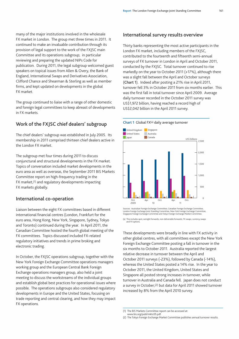
Report The London Foreign Exchange Joint Standing Committee 161
many of the major institutions involved in the wholesaleFX market in London. The group met three times in 2011. Itcontinued to make an invaluable contribution through itsprovision of legal support to the work of the FXJSC mainCommittee and its operations subgroup; in particularreviewing and preparing the updated NIPs Code forpublication. During 2011, the legal subgroup welcomed guestspeakers on topical issues from Allen & Overy, the Bank ofEngland, International Swaps and Derivatives Association,Clifford Chance and Shearman & Sterling as well as memberfirms, and kept updated on developments in the globalFX market.
The group continued to liaise with a range of other domesticand foreign legal committees to keep abreast of developmentsin FX markets.
Work of the FXJSC chief dealers’ subgroup
The chief dealers’ subgroup was established in July 2005. Itsmembership in 2011 comprised thirteen chief dealers active inthe London FX market.
The subgroup met four times during 2011 to discussconjunctural and structural developments in the FX market.Topics of conversation included market developments in theeuro area as well as overseas, the September 2011 BIS MarketsCommittee report on high-frequency trading in theFX market,(1) and regulatory developments impactingFX markets globally.
International co-operation
Liaison between the eight FX committees based in differentinternational financial centres (London, Frankfurt for theeuro area, Hong Kong, New York, Singapore, Sydney, Tokyoand Toronto) continued during the year. In April 2011, theCanadian Committee hosted the fourth global meeting of theFX committees. Topics discussed included FX-relatedregulatory initiatives and trends in prime broking andelectronic trading.
In October, the FXJSC operations subgroup, together with theNew York Foreign Exchange Committee operations managersworking group and the European Central Bank ForeignExchange operations managers group, also held a jointmeeting to discuss the workstreams of the individual groupsand establish global best practices for operational issues wherepossible. The operations subgroups also considered regulatorydevelopments in Europe and the United States, focusing ontrade reporting and central clearing, and how they may impactFX operations.
International survey results overview
Thirty banks representing the most active participants in theLondon FX market, including members of the FXJSC,contributed to the fourteenth and fifteenth semi-annualsurveys of FX turnover in London in April and October 2011,conducted by the FXJSC. Total turnover continued to risemarkedly on the year to October 2011 (+17%), although therewas a slight fall between the April and October surveys(Chart 1). Indeed after posting a 21% rise in April 2011,turnover fell 3% in October 2011 from six months earlier. Thiswas the first fall in total turnover since April 2009. Averagedaily turnover recorded in the October 2011 survey wasUS$1,972 billion, having reached a record high ofUS$2,042 billion in the April 2011 survey.
These developments were broadly in line with FX activity inother global centres, with all committees except the New YorkForeign Exchange Committee posting a fall in turnover in thesix months to October 2011. Australia reported the largestrelative decrease in turnover between the April andOctober 2011 surveys (-23%), followed by Canada (-14%),whereas the United States posted a 14% rise. In the year toOctober 2011, the United Kingdom, United States andSingapore all posted strong increases in turnover, whileturnover in Australia and Canada fell. Japan does not conducta survey in October,(2) but data for April 2011 showed turnoverincreased by 8% from the April 2010 survey.
(1) The BIS Markets Committee report can be accessed at:www.bis.org/publ/mktc05.pdf.
(2) The Tokyo Foreign Exchange Market Committee publishes annual turnover results.
Chart 1 Global FX(a) daily average turnover
0
500
1,000
1,500
2,000
2,500
Oct. Apr. Oct. Apr. Oct.
United Kingdom
United States
Japan
Singapore
Australia
CanadaUS$ billions
2009 10 11
Sources: Australian Foreign Exchange Committee, Canadian Foreign Exchange Committee,London Foreign Exchange Joint Standing Committee, New York Foreign Exchange Committee,Singapore Foreign Exchange Committee and Tokyo Foreign Exchange Market Committee.
(a) This includes spot, outright forwards, non-deliverable forwards, FX swaps, currency swapsand FX options.
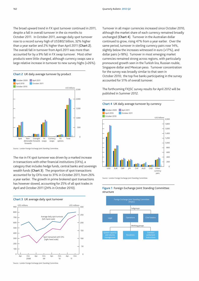
162 Quarterly Bulletin 2012 Q2
The broad upward trend in FX spot turnover continued in 2011,despite a fall in overall turnover in the six months toOctober 2011. In October 2011, average daily spot turnoverrose to a record survey high of US$802 billion, 32% higherthan a year earlier and 2% higher than April 2011 (Chart 2).The overall fall in turnover from April 2011 was more thanaccounted for by a 9% fall in FX swap turnover. Most otherproducts were little changed, although currency swaps saw alarge relative increase in turnover to new survey highs (+26%).
The rise in FX spot turnover was driven by a marked increasein transactions with other financial institutions (OFIs), acategory that includes hedge funds, central banks and sovereignwealth funds (Chart 3). The proportion of spot transactionsaccounted for by OFIs rose to 31% in October 2011, from 26%a year earlier. The growth in prime brokered spot transactionshas however slowed, accounting for 25% of all spot trades inApril and October 2011 (24% in October 2010).
Turnover in all major currencies increased since October 2010,although the market share of each currency remained broadlyunchanged (Chart 4). Turnover in the Australian dollarcontinued to grow, rising 47% from a year earlier. Over thesame period, turnover in sterling currency pairs rose 14%,slightly below the increases witnessed in euro (+17%), anddollar pairs (+18%). Turnover in most emerging marketcurrencies remained strong across regions, with particularlypronounced growth seen in the Turkish lira, Russian rouble,Singapore dollar and Mexican peso. Turnover concentrationfor the survey was broadly similar to that seen inOctober 2010; the top five banks participating in the surveyaccounted for 51% of overall turnover.
The forthcoming FXJSC survey results for April 2012 will bepublished in Summer 2012.
Chart 2 UK daily average turnover by product
0
500
1,000
1,500
2,000
2,500
Spot Non-
deliverable
forwards
Outright
forwards
FX
swaps
Currency
swaps
FX
options
Total
October 2009
April 2010
October 2010
April 2011
October 2011
US$ billions
Source: London Foreign Exchange Joint Standing Committee.
0
50
100
150
200
250
300
0
100
200
300
400
500
600
700
800
900
Apr. Oct. Apr. Oct. Apr. Oct. Apr. Oct.
2008 09 10 11
US$ millions US$ millions
Average daily spot turnover (left-hand scale)
Spot transacted with OFIs
(right-hand scale)
Source: London Foreign Exchange Joint Standing Committee.
Chart 3 UK average daily spot turnover
Chart 4 UK daily average turnover by currency
0
200
400
600
800
1,000
1,200
1,400
1,600
1,800
2,000US$ billions
October 2009
April 2010
October 2010
April 2011
October 2011
USD EUR GBP JPY CHF AUD CAD Othercurrency
pairs
Source: London Foreign Exchange Joint Standing Committee.
Legal Operations Chief dealers
System capacityand volume
management
Foreign Exchange Joint Standing Committee
(FXJSC)
NovationsStandard
settlement
instructions
Subgroups
Working groups
Figure 1 Foreign Exchange Joint Standing Committee:structure

Report The London Foreign Exchange Joint Standing Committee 163
Members of the London Foreign Exchange Joint StandingCommittee as at December 2011
Name Firm/organisation
Brian Welch Association of Corporate Treasurers
Christopher Bae Bank of America Merrill Lynch
Rob Loewy Bank of China
Richard Gill Bank of New York Mellon
Mike Bagguley Barclays
Eric Auld BNP Paribas
Andrew Rogan British Bankers’ Association
James Bindler Citi
Alan Bozian CLS Bank
Vincent Leclercq Crédit Agricole CIB
Martin Wiedmann Credit Suisse
Zar Amrolia Deutsche Bank
Heather Pilley Financial Services Authority
Phil Weisberg FXAll
Nick Burgin Goldman Sachs
Frederic Boillereau HSBC
John Nixon ICAP
Troy Rohrbaugh JPMorgan Chase
Roger Hawes Royal Bank of Scotland
James Potter Tullett Prebon
Alex McDonald Wholesale Markets Brokers’ Association
Graeme Munro JPMorgan Chase, Chair, operations subgroup
Nick Cox BlackRock, Chair, FX investor subgroup
Michael Cross (Chair) Bank of England
Elizabeth Wrigley Bank of England
Grigoria Christodoulou, Jack Garrett-Jones and Sumita Ghosh (Secretariat) Bank of England
Members of the London Foreign Exchange Joint StandingCommittee operations subgroup as at December 2011
Name Firm/organisation
Nigel Brigden Association of Foreign Banks
Michael Douglas Bank of America Merrill Lynch
Barry Harrison Bank of England
Pamela Bald Bank of New York Mellon
Duncan Lord Barclays
Andrew Rogan British Bankers’ Association
Leigh Meyer Citi
Phil Kenworthy CLS Services
Andreas Gaus Credit Suisse
Nick Doddy Deutsche Bank
Catherine Plant Goldman Sachs
Mike Neale HSBC
Anna Box ISDA
Andrew Harvey Morgan Stanley
Stephen Nankivell Nomura
Jeremy Hill Royal Bank of Scotland
Ian Cowell State Street
Joe Halberstadt SWIFT
Jane Collins Thomson Reuters
Daniel Haid UBS
Graeme Munro (Chair) JPMorgan Chase
Grigoria Christodoulou, Jack Garrett-Jones, Sumita Ghosh and Richard Hailston (Secretariat) Bank of England
Members of the London Foreign Exchange Joint StandingCommittee chief dealers’ subgroup as at December 2011
Name Firm/organisation
Ryuichi Takami Bank of Tokyo-Mitsubishi UFJ
Bob de Groot BNP Paribas
Bernie Kipping Commonwealth Bank of America
Danny Wise Credit Suisse
Angus Greig Deutsche Bank
Jon Pierce Goldman Sachs
Stuart Scott HSBC
Richard Usher JPMorgan Chase
Ed Monaghan Royal Bank of Canada
Roger Hawes Royal Bank of Scotland
Chris Freeman State Street
Niall O’Riordan UBS
Martin Mallett (Chair) Bank of England
James O’Connor Bank of England
Members of the London Foreign Exchange Joint StandingCommittee legal subgroup as at December 2011
Name Firm/organisation
Gaynor Wood Bank of America
Richard Haynes Citi
Simon Goldsworthy Deutsche Bank
Carl Husselman Deutsche Bank
Anne Moore-Williams Financial Services Authority
Dan Parker Goldman Sachs
Mehboob Lakhany HSBC
Christian Bettley HSBC
Patrick Palmer JPMorgan Chase
Barra Little Morgan Stanley
Alex Bouchier Royal Bank of Scotland
Alistair Cleverly Standard Chartered
Martin Oakley Thomson Reuters
Chris Allen (Chair) Barclays
Jacqueline Joyston-Bechal (Secretariat) Bank of England
Tables of membership at end-2011


Quarterly Bulletin Speeches 165
Speeches
166 Quarterly Bulletin 2012 Q2
A short summary of speeches and ad hoc papers made by Bank personnel since publication of the previous Bulletin arelisted below.
Costly capital and the risk of rare disastersBen Broadbent, Monetary Policy Committee member,May 2012.
www.bankofengland.co.uk/publications/Documents/speeches/2012/speech581.pdf
In a speech delivered at Bloomberg in London, Ben Broadbentargued that investors’ fears about downside risks and thepossibility of an extreme economic outcome had driven a risein the premium for risky investment, however it is financed.This will have particularly marked effects on hurdle rates forirreversible, sunk-cost investments that are necessary toimprove productivity. Therefore, he suggested that thosefears, in turn, have affected the growth of UK activity.However, if those fears of downside risks were to recede, thiscould have pretty powerful effects on output — potential aswell as actual — in a positive direction. He concluded bysaying that were the (still unlikely) worst-case risks in theeuro area to be realised, then our own monetary policy wouldagain play its part in mitigating the impact. That said, heacknowledged that these interventions have their limits.
Monetary policy and the damaged economy David Miles, Monetary Policy Committee member, May 2012.
www.bankofengland.co.uk/publications/Documents/speeches/2012/speech576.pdf
In this speech, delivered at the Society of Business EconomistsAnnual Conference, Professor Miles explained why he believedthere was a case for making monetary policy moreexpansionary, even when inflation had surprised repeatedly onthe upside. He argued that inflation inertia could be explainedby two factors: lower (but still substantial) spare capacity inthe economy; and a lower impact of spare capacity oninflation. The weakened link between spare capacity andinflation meant that the costs and benefits of bringing inflationback to target faster or slower have changed. On the one side,a lot of spare capacity would be needed to reduce inflationquickly — and this meant that capital would be used less andunemployment would be higher, which would be costly interms of welfare. On the other side, stimulating demandwould put less pressure on inflation. In addition, theeconomy’s capacity risked falling the longer output remainedbelow potential. Professor Miles concluded that these reasonsmade an exceptionally expansionary monetary policyappropriate.
What is the FPC for?Alastair Clark, Financial Policy Committee member, May 2012.
www.bankofengland.co.uk/publications/Documents/speeches/2012/speech575.pdf
In this speech, Alastair Clark discussed the objectives andinstruments of the Financial Policy Committee (FPC). Alastairnoted that the objective of the FPC — protecting andenhancing the resilience of the financial system — was meantto help avoid crises, not to manage them: it was a fireprevention officer, not the fire brigade. Delivering thismacroprudential objective would be challenging; there was nouniversally accepted definition of financial stability, still lessagreement on how to translate financial stability into a targetfor policymakers. And there were also possible tensions withother areas of public policy, in particular the objective of tryingto promote economic growth. Alastair highlighted that usingpolicy instruments for macroprudential purposes andcalibrating their impact was now, and was likely to remain,partly a matter of experiment. There was relatively littleempirical evidence on the effect which most potentially usefulinstruments had on financial stability.
The future of UK banking — challenges ahead for promoting astable sectorAndrew Bailey, Executive Director, May 2012.
www.bankofengland.co.uk/publications/Documents/speeches/2012/speech574.pdf
In this speech, Andrew Bailey discussed the current conditionsfacing retail banks from a prudential perspective. Andrewspoke about the pressures on interest margins, and contrastedthis with previous recessions where more of the pressure camefrom loan losses in the context of higher nominal interestrates.
Andrew also spoke about the risks UK banks face from theeuro area and the importance of continuing to developcontingency plans in the event of countries leaving the area.UK banks should take actions to maintain adequate capitalagainst foreseeable risks, but it is important that inencouraging such actions, the authorities do not createunnecessary uncertainty.
Andrew ended by arguing that the public should be told whatthey pay for the services they receive from banks. So-called‘free in-credit banking’ creates an illusion which does notmatch the reality.
Bank of England speeches
Quarterly Bulletin Speeches 167
Pension funds and quantitative easingCharlie Bean, Deputy Governor, May 2012.
www.bankofengland.co.uk/publications/Documents/speeches/2012/speech573.pdf
In a speech to the National Association of Pension Funds’ LocalAuthority Conference, Deputy Governor Charlie Beandiscussed the impact on pension funds of factors such as thefall in equity prices after the collapse of Lehman Brothers andthe fall in long-term interest rates, in part as a result ofquantitative easing (QE). Bearing in mind that QE raises theprices of other assets as well as depressing gilt yields, he foundthat the path of the deficit for a pension fund starting 2007 inbalance, would have been broadly the same with and withoutQE. For a fund that was initially underfunded by 30%,however, QE would have widened the deficit by about10 percentage points. Consequently the impact of QE dependscritically on the initial position of the fund. He also noted thata variety of factors were likely to keep gilt yields low for sometime yet.
Articles on the framework for macroprudential policy Paul Tucker, Deputy Governor, March-May 2012.
www.bankofengland.co.uk/publications/Documents/speeches/2012/speech580.pdf (Co-authored with Andreas Dombret)
www.bankofengland.co.uk/publications/Documents/speeches/2012/speech578.pdf
www.bankofengland.co.uk/publications/Documents/speeches/2012/speech562.pdf
In these three articles (two published in the Financial Times andone in the Eurofi High Level Newsletter), Paul Tucker set outthe need for countries to have a macroprudential policyframework. Though central banks around the world broadlydelivered price stability in the run-up to the crisis, the financialsystem expanded rapidly without check. The consequenceshave been dreadful.
While international work is under way to strengthenmicro-regulatory regimes, any reforms will eventually beovertaken by structural change or by bursts of misplacedexuberance. Policymakers will need a rich macroprudentialtoolkit, with room temporarily to adjust regulatoryrequirements to head off future threats to the resilience of thefinancial system.
Mr Tucker stressed that, within the EU, national flexibility andregional differentiation are important. Credit cycles are notalways synchronised. National macroprudential policies couldbe particularly useful within the euro area, where one settingfor monetary policy is not always guaranteed to suit financialconditions everywhere.
Currency in search of confidenceRobert Jenkins, Financial Policy Committee member, May 2012.
www.bankofengland.co.uk/publications/Documents/speeches/2012/speech572.pdf
In this article, published in The Times, Robert Jenkinshighlighted how a lack of confidence in the viability of theeurozone has brought risks associated with cross-borderlending to the fore. Robert noted that the creation of theeuro area was supposed to eliminate cross-border risk forlending within it, but that current concerns threatened toundermine this principle. While banks can plan for andmanage cross-border risks in the long run by growing localdeposits to match local loans, Robert noted that in theshort run they may instead seek to cut, or at least limit,local loans — and thus exacerbate local deleveraging.
On counterparty riskAndrew Haldane, Executive Director for Financial Stability,May 2012.
www.bankofengland.co.uk/publications/Documents/speeches/2012/speech571.pdf
In this paper, Andrew Haldane examined the vulnerability offinancial structures to counterparty concerns. Sketching amodel of financial structure of the unsecured money market,Andrew demonstrated that management of counterpartycredit risk was inadequate during the financial crisis. Andrewidentified three possible solutions that have been proposed tomitigate such risks in the future: improved network visibility tounderstand credit chains; the clearing of transactions centrallyto improve transparency and reduce intra-financial systemdebt; and building protection against counterparty defaultthrough higher capital and margining requirements. Takentogether, there is an enormous amount still to be done beforecounterparty risk is properly recognised and managed. Thegood news is that the technological frontier of counterpartyrisk management is being pushed out by financial firms, centralcounterparties and systemic risk regulators.
Bank executives: now we have your attention…Robert Jenkins, Financial Policy Committee member,May 2012.
www.bankofengland.co.uk/publications/Documents/speeches/2012/speech570.pdf
In this article, published in Financial News, Robert Jenkinscalled on bank shareholders to direct their protests at bankBoards by calling for the use of risk-adjusted performancemetrics that are more closely aligned with shareholder value.The focus on short-term return on equity over recent years
168 Quarterly Bulletin 2012 Q2
created incentives to increase returns — which many banksmanaged some of the time — and to reduce equity — whichmany banks did all of the time; this had resulted in short-termgains for employees at the expense of long-term shareholdervalue. Robert also noted that the higher cost of capital facingsome banks is not necessarily the result of rising capitalrequirements but more to do with the market’s new-foundunderstanding of the risks that banks run and the prospectiveremoval of government subsidies and safety nets.
Basel II proved to be inadequate, so are the new rules really‘too severe’?Robert Jenkins, Financial Policy Committee member, May 2012.
www.bankofengland.co.uk/publications/Documents/speeches/2012/speech569.pdf
In this article, published in The Independent, Robert Jenkinshighlighted how the Basel II capital regulations provedinadequate to ensure that banks held enough capital tosupport a given level of risk. Sovereign debt and seniortranches of collateralised debt obligations are cited asexamples of bank exposures that proved to be a lot riskier thanimplied by the Basel framework. Robert concluded that ‘timewill tell’ whether the strengthening of bank capital regulationsunder Basel III will prove sufficient and that it is surely prudentto err on the side of caution rather than assuming that bankersor regulators can predict the future with certainty.
Resolution: a progress reportPaul Tucker, Deputy Governor, May 2012.
www.bankofengland.co.uk/publications/Documents/speeches/2012/speech568.pdf
In this speech, Paul Tucker, Chair of the Financial StabilityBoard’s Resolution Steering Group, provided a progress report on global planning for resolution regimes aimed ataddressing the problem of ‘too big to fail’. Progress in this area was not optional: if risks in banking were notincorporated into the yields of bonds issued by banks, theywould end up being reflected in higher sovereign borrowingcosts. Specific strategies were needed to resolve complexsystemically important financial institutions (SIFIs). If therewas enough debt issued by the firm’s holding company, onesuch strategy could be to write off the equity and parts of thedebt, converting some of the residual debt into equity. In that case, a SIFI could be recapitalised through ‘bail-in’ without the complexity of separating its business lines. Some authorities were working on how to operationalise thisstrategy. In other circumstances, where a giant commercialbank was funded by insured deposits, the resolution strategymight revolve around using the resources of the relevantdeposit insurers. In all cases, the necessary tools had to be in
the statutory resolution regime. The forthcoming EU directivewas crucial to this.
What we know now: the BoE’s past 15 years Charlie Bean, Deputy Governor, May 2012.
www.bankofengland.co.uk/publications/Documents/speeches/2012/speech577.pdf
In this article, Deputy Governor Charlie Bean examined thelessons for monetary policy from the MPC’s first fifteen years.First, hitting the inflation target did not guarantee economicstability. The answer, though, was not to jettison the inflationtarget but rather to utilise regulatory tools of the sortconsidered by the Bank’s new Financial Policy Committee.Second, it was easier than expected to enter unchartedterritory. During the first decade of the MPC, there seemedlittle danger of Bank Rate approaching zero, let alone of theMPC resorting to quantitative easing. The financial crisischanged that. Third, a long period of abnormal monetarypolicy settings had undesirable distributional side effects andcould strain support for a central bank’s actions. But thehighly stimulatory policy stance should help return theeconomy to an even keel, which was the best medicine for all.
The 2012 BBC Today Programme LectureSir Mervyn King, Governor, May 2012.
www.bankofengland.co.uk/publications/Documents/speeches/2012/speech567.pdf
In his radio speech, the first by a Bank of England Governorsince Montagu Norman in 1939, the Governor reflected onthree questions: what went wrong in the run-up to thefinancial crisis; the lessons learnt; and the reforms needed toprevent future crises.
The Governor began by noting the period of steady growth,and low and stable unemployment and inflation, in the yearspreceding the crisis. Though overall growth had beensustainable, fragilities had built up in the banking system, anissue the Bank raised repeatedly — though perhaps notforcefully enough — in its publications. Fuelled by an implicittaxpayer guarantee, banks became highly leveraged and toobig to fail. The resulting lack of confidence in the bankingsystem prompted significant injections of central bankliquidity and government recapitalisation of two of theUnited Kingdom’s largest banks.
The Governor reflected on the lessons learnt from the crisis.Three areas of reform would be important. First, bankregulation, where the Financial Policy Committee would guardagainst the big risks to the financial system. Second, enactinga resolution mechanism would ensure that badly run banksfailed safely, without causing damage to depositors. Third,
Quarterly Bulletin Speeches 169
restructuring the banking system by enacting the proposalsmade by the Independent Commission on Banking to separateessential banking services from riskier trading activities.Regulation, resolution and restructuring of the banks were thethree Rs of a new approach to make banking, and so theUK economy, safer. They would be central to the work of theBank of England.
The Governor concluded by emphasising the importance oflooking to the future, and to the economic possibilities for thegrandchildren of today’s generation. To give them theprospect of economic stability, it was vital to reform thethree Rs of the financial system. There was a historicopportunity, and a duty, to do that.
Shadow banking: thoughts for a possible policy agendaPaul Tucker, Deputy Governor, April 2012.
www.bankofengland.co.uk/publications/Documents/speeches/2012/speech566.pdf
In this speech, Paul Tucker set out a possible ten-point policyagenda to address risks to stability from shadow banking. Theobjective should not be to curb non-bank finance, but torecognise where intermediation is banking in substance or inthe systemic risks it creates. Shadow banking that wassponsored or operated by banks should be consolidated on tobanks’ balance sheets. Committed credit lines to financialcompanies should attract a high liquidity charge. Reformswere needed to improve the resilience of money market funds.Other lending businesses that were materially financed byshort-term debt should be subject to bank-type regulation.Only banks should be able to use client moneys andunencumbered assets to finance their own business to amaterial extent. Reforms were needed in securities lendingand repo markets. A trade repository could improvetransparency. The authorities should also be able to step inand set and vary minimum haircut and margin levels.
Financial arms racesAndrew Haldane, Executive Director for Financial Stability,April 2012.
www.bankofengland.co.uk/publications/Documents/speeches/2012/speech565.pdf
In this speech, Andrew Haldane noted that competitive battlesfor dominance in many fields led to arms races and negativeexternalities. Andrew discussed three examples of arms racesin the financial sector: races for return, races for speed andraces for safety. The race for returns on capital led to bankssignificantly increasing their leverage, leading to a riskyequilibrium and sowing the seeds of the financial crisis. Theincreasing dominance of so-called high-frequency trading wasa race for speed and led to a huge increase in order
cancellations, order congestion and periods of dramaticdisappearance of liquidity. Post-crisis, the race for safety ledto a greater proportion of banks’ refinancing done on a securedbasis, increasing asset encumbrance. At high levels of assetencumbrance the financial system as a whole may be riskier asit is more susceptible to procyclical swings in the underlyingvalue of bank balance sheets. Competitive races can generateunhealthy outcomes for the system as a whole. In financethese tragedies of the commons are, if anything, more likelythan in other fields. Macroprudential policy, in the United Kingdom executed via the Financial Policy Committee,has been set up precisely to deal with these systemicphenomena.
Credit conditions for firms: stability and monetary policyPaul Tucker, Deputy Governor, April 2012.
www.bankofengland.co.uk/publications/Documents/speeches/2012/speech564.pdf
In this speech, Paul Tucker addressed some issues facingbusinesses as the economy rebalances and the financialsystem rebuilds. Bank lending conditions were likely to remaintight for some time. Some larger companies were not heavilyreliant on bank finance given access to internal funds and tocapital markets. They could support smaller firms throughdirect lending or by setting up programmes to allow suppliersto borrow against unpaid invoices. The revival of oldinstruments such as bankers’ acceptances, or innovationscreating new instruments, could also support bank lending tobusiness. The Monetary Policy Committee would continue tosupport demand so long as that was consistent with bringinginflation back to the 2% target in the medium term.Underlying growth was probably better than headline numberswould suggest. Inflation was likely to fall back more slowlythan had been expected, which was potentially problematic.
Liquidity support from the Bank of England: the DiscountWindow FacilityPaul Fisher, Executive Director for Markets, March 2012.
www.bankofengland.co.uk/publications/Documents/speeches/2012/speech561.pdf
Since the start of the crisis in 2007, the Bank has reformed andredesigned much of its Sterling Monetary Framework. One ofthe most significant changes to the Bank’s arrangements forthe provision of liquidity support was the introduction of aDiscount Window Facility (DWF) in 2008. In this speech,Paul Fisher explained the principles underpinning the design ofthe DWF, as well as recent developments. Those includedencouraging banks to ‘pre-position’ collateral — so that it neednot be assessed at short notice in the event of a sudden andunexpected need to borrow. By March 2012, £265 billion hadbeen pre-positioned, giving a drawing capacity of £160 billion.
170 Quarterly Bulletin 2012 Q2
Paul expected that amount to increase further over time. Paulalso described the Bank’s new Extended Collateral Term RepoFacility, introduced in December 2011 as a contingentoperation, which could provide liquidity against illiquidcollateral pre-positioned in the DWF, through a market-wideauction.
Why is their recovery better than ours? (Even though neitheris good enough)Adam Posen, Monetary Policy Committee member, March 2012.
www.bankofengland.co.uk/publications/Documents/speeches/2012/speech560.pdf
In this speech, Dr Posen explained the superior recovery in theUnited States to that of the United Kingdom from the globalfinancial crisis so far. He noted that the two economiessuffered similar shocks and pursued similar monetaryresponses. The respective responses of net trade andautomatic stabilisers only add to the gap in GDP to beexplained. Dr Posen pointed to the stronger privateinvestment and consumption recovery in the United Statesand argued that the former can be explained by lesseravailability and greater misallocation of bank credit in theUK economy as well as its greater exposure to the euro area.He put the difference in consumption performance to greaterfiscal austerity in the United Kingdom and a greater impact ofenergy costs on UK households. The relative inflationperformance can be explained by one-off price-level shocks inthe United Kingdom, so inflation expectations continue to bewell anchored in both economies. Most of these differencesare likely to diminish, but the relative inefficiency of theUnited Kingdom’s allocation of capital to business remains aconcern.
Government debt and unconventional monetary policyDavid Miles, Monetary Policy Committee member, March 2012.
www.bankofengland.co.uk/publications/Documents/speeches/2012/speech559.pdf
In this speech, David Miles outlined why he feels concernsabout the monetisation of government debt by central banksare misplaced. In the United Kingdom, those concerns havebecome more acute over the past few years as public debt hasincreased, and as the Bank of England has purchased asignificant amount of government debt. Professor Milesargued that the purchases of government bonds were notundertaken to finance the Government’s fiscal deficits. Rather,they were undertaken in order to loosen monetary policy andoffset recessionary forces that might otherwise have created alasting depression which could have generated deflation.Other major central banks have carried out similar balance
sheet expansions in response to the impact of the financialcrisis. Professor Miles noted that the tricky task ahead forthose central banks is to know for how long to keep monetarypolicy exceptionally expansionary; not because of anypractical difficulties in unwinding asset purchases, but becauseof the much more fundamental and timeless challenge ofassessing the outlook for the economy and judging theappropriate monetary stance.
Crisis and crash: lessons for regulationMichael Cohrs, Financial Policy Committee member, March 2012.
www.bankofengland.co.uk/publications/Documents/speeches/2012/speech558.pdf
This speech outlined the lessons for regulators from thefinancial crisis of 2008, for which Michael Cohrs had afront-row seat, as the (then) co-head of corporate andinvestment banking at Deutsche Bank. Michael suggested itwas clear (in hindsight) that the premise of ‘efficient’ marketbehaviour, the structure of the banking industry, and theregulatory framework, were unsuitable prior to 2008. Oneparticular failure of regulation was that there was no singleinstitution mandated with the responsibility, and powers, tomonitor the system as a whole, identify potentiallydestabilising trends, and respond to them with concertedactions. The changes to financial sector regulation in theUnited Kingdom, proposed in June 2010, gave thisresponsibility to the Financial Policy Committee (FPC), whichwas currently in interim form. Michael noted that the prize forthe FPC fulfilling its mandate — focusing on protecting andenhancing the resilience of the UK financial system — wouldbe huge, given the sizable and persistent impact of financialcrises on real activity.
Rebalancing the supply side of the UK economy: what; how;and issues for monetary policySpencer Dale, Executive Director and Chief Economist, March 2012.
www.bankofengland.co.uk/publications/Documents/speeches/2012/speech554.pdf
In a speech to mark the centenary of the Department ofEconomics at the University of Aberystwyth, Spencer Dalediscussed the imperative of rebalancing the supply side of theUK economy, and explained two reasons why this processposes significant challenges for UK monetary policy.
The first policy challenge Spencer Dale highlighted was thatrebalancing can be associated with a slowing in the growth ofthe supply capacity of the economy, including via adetachment of the long-term unemployed from the labourmarket. While Mr Dale was convinced that the substantial
Quarterly Bulletin Speeches 171
loosening of monetary policy over recent years was necessaryto prevent an even deeper recession, the second challenge henoted was that this loosening may also serve to blunt some ofthe incentives driving the rebalancing of the economy. Itencourages people to spend more and save less, and delays thereallocation of capital and labour to more productive uses.This leaves monetary policy makers facing a delicate trade-offbetween short-term support and stifling longer-term change.
Spencer Dale also explained that the Monetary PolicyCommittee (MPC) has recently begun to use a new forecastingplatform to produce inflation projections, consisting of arelatively simple central organising model and a surroundingsuite of alternative models. Mr Dale stressed that theintroduction of this platform did not, in itself, imply anychanges to the MPC’s forecasts or how they set policy.
DeleveragingBen Broadbent, Monetary Policy Committee member, March 2012.
www.bankofengland.co.uk/publications/Documents/speeches/2012/speech553.pdf
In this speech, Ben Broadbent considered what the build-up ofdebt by UK firms and households prior to the financial crisiscan tell us about the prospects for a sustainable recovery, thekey risks currently facing the economy, and the implicationsfor policymakers. He argued that non-financial domesticleverage does not need to return to some historical ‘norm’,because UK firms and households accumulated assets as wellas liabilities before the crisis, in response to the decline in reallong-term interest rates. Furthermore, there is no empiricalevidence that links relative levels of debt to output growth. Hesuggested that an alternative explanation for the severe creditcrunch was the spillover effects from the losses UK bankssustained on non-UK assets. The prospects of a sustainablerecovery are therefore more closely tied to developments inthe UK banking sector than the domestic non-financial sector.This means that a withdrawal of monetary accommodationcould begin even if domestic debt to income ratios remain wellabove historical averages.


Quarterly Bulletin Appendices 173
Appendices
174 Quarterly Bulletin 2012 Q2
The articles and speeches that have been published recently in the Quarterly Bulletin are listed below. Articles from May 1994 onwards are available on the Bank’s website at:
www.bankofengland.co.uk/publications/Pages/quarterlybulletin/default.aspx.
Articles and speechesSpeeches are indicated by (S)
2007 Q4– Household debt and spending: results from the 2007 NMG
Research survey– The macroeconomic impact of higher energy prices on the
UK economy– Decomposing corporate bond spreads– The foreign exchange and over-the-counter derivatives
markets in the United Kingdom– The Governor’s speech in Northern Ireland (S)– Current monetary policy issues (S)– The global economy and UK inflation (S)– Trends in European labour markets and preferences over
unemployment and inflation (S)– Fear, unemployment and migration (S)– Risk, uncertainty and monetary policy (S)– New markets and new demands: challenges for central
banks in the wholesale market infrastructure (S)– A tale of two shocks: global challenges for UK monetary
policy (S)
2008 Q1– Capital inflows into EMEs since the millennium: risks and
the potential impact of a reversal– Recent developments in portfolio insurance– The Agents’ scores: a review– The impact of low-cost economies on UK import prices– The Society of Business Economists’ survey on MPC
communications– The Governor’s speech in Bristol (S)– The impact of the financial market disruption on the
UK economy (S)– The return of the credit cycle: old lessons in new markets (S)– Money and credit: banking and the macroeconomy (S)– Financial markets and household consumption (S)
2008 Q2– Public attitudes to inflation and interest rates– Recent advances in extracting policy-relevant information
from market interest rates– How do mark-ups vary with demand?– On the sources of macroeconomic stability
– A review of the work of the London Foreign Exchange Joint Standing Committee in 2007
– Sovereign wealth funds and global imbalances (S)– Monetary policy and the financial system (S)– Inflation and the global economy (S)– Does sterling still matter for monetary policy? (S)– Strengthening regimes for controlling liquidity risk: some
lessons from the recent turmoil (S)– Inflation, expectations and monetary policy (S)
2008 Q3– Market expectations of future Bank Rate– Globalisation, import prices and inflation: how reliable are
the ‘tailwinds’?– How has globalisation affected inflation dynamics in the
United Kingdom?– The economics of global output gap measures– Banking and the Bank of England (S)– The Governor’s speech at the Mansion House (S)– A tale of two cycles (S)– The financial cycle and the UK economy (S)– The credit crisis: lessons from a protracted ‘peacetime’ (S)– Financial innovation: what have we learnt? (S)– Global inflation: how big a threat? (S)– Remarks on ‘Making monetary policy by committee’ (S)
2008 Q4– The financial position of British households: evidence from
the 2008 NMG Research survey– Understanding dwellings investment– Price-setting behaviour in the United Kingdom– Monetary Policy Roundtable
2009 Q1– Price-setting behaviour in the United Kingdom: a microdata
approach– Deflation
2009 Q2– Quantitative easing– Public attitudes to inflation and monetary policy– The economics and estimation of negative equity– A review of the work of the London Foreign Exchange Joint
Standing Committee in 2008
2009 Q3– Global imbalances and the financial crisis– Household saving– Interpreting recent movements in sterling– What can be said about the rise and fall in oil prices?
Contents of recent Quarterly Bulletins
Quarterly Bulletin Appendices 175
– Bank of England Systemic Risk Survey– Monetary Policy Roundtable
2009 Q4– The financial position of British households: evidence from
the 2009 NMG survey– Accounting for the stability of the UK terms of trade– Recent developments in pay settlements
2010 Q1– Interpreting equity price movements since the start of the
financial crisis– The Bank’s balance sheet during the crisis– Changes in output, employment and wages during
recessions in the United Kingdom– Monetary Policy Roundtable
2010 Q2– Collateral risk management at the Bank of England– The impact of the financial crisis on supply– Public attitudes to inflation and monetary policy– A review of the work of the London Foreign Exchange Joint
Standing Committee in 2009
2010 Q3– Understanding the price of new lending to households– Interpreting the world trade collapse– What can we learn from surveys of business expectations?– Residential property auction prices– Chief Economists’ Workshop: state-of-the-art modelling for
central banks– Monetary Policy Roundtable
2010 Q4– The history of the Quarterly Bulletin– Index of articles 1960–2010– The UK recession in context — what do three centuries of
data tell us?– The Bank’s money market framework– Managing the circulation of banknotes– Understanding the weakness of bank lending– Evolution of the UK banking system– The financial position of British households: evidence from
the 2010 NMG Consulting survey– The foreign exchange and over-the-counter interest rate
derivatives markets in the United Kingdom– Global finance after the crisis
2011 Q1– Understanding the recent weakness in broad money growth– Understanding labour force participation in the
United Kingdom– Global imbalances: the perspective of the Bank of England– China’s changing growth pattern– Monetary Policy Roundtable
2011 Q2– Assessing the risk to inflation from inflation expectations– International evidence on inflation expectations during
Sustained Off-Target Inflation episodes– Public attitudes to monetary policy and satisfaction with
the Bank– The use of foreign exchange markets by non-banks– Housing equity withdrawal since the financial crisis– Using internet search data as economic indicators– A review of the work of the London Foreign Exchange Joint
Standing Committee in 2010
2011 Q3– The United Kingdom’s quantitative easing policy: design,
operation and impact– Bank resolution and safeguarding the creditors left behind– Developments in the global securities lending market– Measuring financial sector output and its contribution to
UK GDP– The Money Market Liaison Group Sterling Money Market
Survey– Monetary Policy Roundtable
2011 Q4– Understanding recent developments in UK external trade– The financial position of British households: evidence from
the 2011 NMG Consulting survey– Going public: UK companies’ use of capital markets– Trading models and liquidity provision in OTC derivatives
markets
2012 Q1– What might be driving the need to rebalance in the
United Kingdom?– Agents’ Special Surveys since the start of the financial crisis– What can the oil futures curve tell us about the outlook for
oil prices?– Quantitative easing and other unconventional monetary
policies: Bank of England conference summary– The Bank of England’s Special Liquidity Scheme– Monetary Policy Roundtable
2012 Q2– How has the risk to inflation from inflation expectations
evolved?– Public attitudes to monetary policy and satisfaction with
the Bank– Using changes in auction maturity sectors to help identify
the impact of QE on gilt yields– UK labour productivity since the onset of the crisis — an
international and historical perspective– Considering the continuity of payments for customers in a
bank’s recovery or resolution– A review of the work of the London Foreign Exchange Joint
Standing Committee in 2011
176 Quarterly Bulletin 2012 Q2
The Bank of England publishes information on all aspects of its work in many formats. Listed below are some of themain Bank of England publications. For a full list, please referto our website:
www.bankofengland.co.uk/publications/Pages/default.aspx.
Working papers
An up-to-date list of working papers is maintained on the Bank of England’s website at:
www.bankofengland.co.uk/publications/Pages/workingpapers/default.aspx
where abstracts of all papers may be found. Papers publishedsince January 1997 are available in full, in portable documentformat (PDF).
No. 440 Time-varying volatility, precautionary saving andmonetary policy (October 2011)Michael Hatcher
No. 441 An estimated DSGE model: explaining variation interm premia (December 2011)Martin M Andreasen
No. 442 The impact of QE on the UK economy — somesupportive monetarist arithmetic (January 2012)Jonathan Bridges and Ryland Thomas
No. 443 Assessing the economy-wide effects of quantitativeeasing (January 2012)George Kapetanios, Haroon Mumtaz, Ibrahim Stevens andKonstantinos Theodoridis
No. 444 Asset purchase policy at the effective lower boundfor interest rates (January 2012)Richard Harrison
No. 445 Does macropru leak? Evidence from a UK policyexperiment (January 2012)Shekhar Aiyar, Charles W Calomiris and Tomasz Wieladek
No. 446 The business cycle implications of banks’ maturitytransformation (March 2012)Martin M Andreasen, Marcelo Ferman and Pawel Zabczyk
No. 447 Implicit intraday interest rate in the UK unsecuredovernight money market (March 2012)Marius Jurgilas and Filip Žikeš
No. 448 Non-rational expectations and the transmissionmechanism (May 2012)Richard Harrison and Tim Taylor
No. 449 Misperceptions, heterogeneous expectations andmacroeconomic dynamics (May 2012)Richard Harrison and Tim Taylor
No. 450 Forecasting UK GDP growth, inflation and interestrates under structural change: a comparison of models withtime-varying parameters (May 2012)Alina Barnett, Haroon Mumtaz and Konstantinos Theodoridis
No. 453 Neutral technology shocks and employmentdynamics: results based on an RBC identification scheme (May 2012)Haroon Mumtaz and Francesco Zanetti
No. 454 Fixed interest rates over finite horizons (May 2012)Andrew P Blake
External MPC Unit discussion papers
The MPC Unit discussion paper series reports on researchcarried out by, or under supervision of, the external membersof the Monetary Policy Committee. Papers are available fromthe Bank’s website at:
www.bankofengland.co.uk/publications/Pages/externalmpcpapers/default.aspx.
The following papers have been published recently:
No. 34 How flexible can inflation targeting be and still work?(October 2011)Adam Posen and Ken Kuttner
No. 35 Demographics, house prices and mortgage design(March 2012)David Miles
Monetary and Financial Statistics
Monetary and Financial Statistics (Bankstats) contains detailedinformation on money and lending, monetary and financialinstitutions’ balance sheets, banks’ income and expenditure,analyses of bank deposits and lending, external business ofbanks, public sector debt, money markets, issues of securities,financial derivatives, interest and exchange rates, explanatorynotes to tables and occasional related articles.
Bank of England publications
Quarterly Bulletin Appendices 177
Bankstats is published on a monthly basis, free of charge, onthe Bank’s website at:
www.bankofengland.co.uk/statistics/Pages/bankstats/default.aspx.
Further details are available from: Leslie Lambert, Monetaryand Financial Statistics Division, Bank of England: telephone 020 7601 4544; fax 020 7601 3208; email [email protected].
Articles that have been published in recent issues of Monetary and Financial Statistics can also be found on theBank’s website at:
www.bankofengland.co.uk/statistics/Pages/ms/articles.aspx.
Financial Stability Report
The Financial Stability Report is published twice a year underthe guidance of the interim Financial Policy Committee (FPC).It covers the Committee’s assessment of the outlook for thestability and resilience of the financial sector at the time ofpreparation of the Report, and the policy actions it advises toreduce and mitigate risks to stability. The Bank of Englandintends this publication to be read by those who areresponsible for, or have interest in, maintaining and promotingfinancial stability at a national or international level. It is ofespecial interest to policymakers in the United Kingdom andabroad; international financial institutions; academics;journalists; market infrastructure providers; and financialmarket participants. It is available at a charge, fromPublications Group, Bank of England, Threadneedle Street,London, EC2R 8AH and on the Bank’s website at:
www.bankofengland.co.uk/publications/Pages/fsr/default.aspx.
Payment Systems Oversight Report
The Payment Systems Oversight Report provides an account ofhow the Bank is discharging its responsibility for oversight ofrecognised UK payment systems. Published annually, theOversight Report identifies the most significant paymentsystem risks to financial stability and assesses progress inreducing these risks. Copies are available on the Bank’swebsite at:
www.bankofengland.co.uk/publications/Pages/psor/default.aspx.
Handbooks in central banking
The series of Handbooks in central banking provide concise,balanced and accessible overviews of key central bankingtopics. The Handbooks have been developed from studymaterials, research and training carried out by the Bank’sCentre for Central Banking Studies (CCBS). The Handbooks aretherefore targeted primarily at central bankers, but are likely tobe of interest to all those interested in the various technicaland analytical aspects of central banking. The Handbook seriesalso includes ‘Technical Handbooks’ which are aimed more atspecialist readers and often contain more methodologicalmaterial than the Handbooks, incorporating the experiencesand expertise of the author(s) on topics that address theproblems encountered by central bankers in their day-to-daywork. All the Handbooks are available via the Bank’s websiteat:
www.bankofengland.co.uk/education/Pages/ccbs/handbooks/default.aspx.
The framework for the Bank of England’soperations in the sterling money markets (the ‘Red Book’)
The ‘Red Book’ describes the Bank of England’s framework forits operations in the sterling money markets, which is designedto implement the interest rate decisions of the MonetaryPolicy Committee while meeting the liquidity needs, and socontributing to the stability of, the banking system as a whole.It also sets out the Bank’s specific objectives for theframework, and how it delivers those objectives. Theframework was introduced in May 2006. The ‘Red Book’ isavailable at:
www.bankofengland.co.uk/markets/Documents/money/publications/redbookjune2012.pdf.
The Bank of England Quarterly Model
The Bank of England Quarterly Model, published in January 2005, contains details of the new macroeconomicmodel developed for use in preparing the Monetary PolicyCommittee’s quarterly economic projections, together with acommentary on the motivation for the new model and theeconomic modelling approaches underlying it.
www.bankofengland.co.uk/publications/Pages/other/beqm/default.aspx.
178 Quarterly Bulletin 2012 Q2
Cost-benefit analysis of monetary andfinancial statistics
The handbook describes a cost-benefit analysis (CBA)framework that has been developed within the Bank to ensurea fair balance between the benefits derived from good-qualitystatistics and the costs that are borne by reporting banks.Although CBA is a well-established approach in other contexts,it has not often been applied to statistical provision, sotechniques have had to be adapted for application to theBank’s monetary and financial statistics. The handbook alsodiscusses how the application of CBA has enabled cuts in boththe amount and the complexity of information that is requiredfrom reporting banks.
www.bankofengland.co.uk/statistics/Pages/about/cba.aspx.
Credit Conditions Survey
As part of its mission to maintain monetary stability andfinancial stability, the Bank needs to understand trends anddevelopments in credit conditions. This survey for bank andnon-bank lenders is an input to this work. Lenders are askedabout the past three months and the coming three months.The survey covers secured and unsecured lending tohouseholds and small businesses; and lending to non-financialcorporations, and to non-bank financial firms. Copies areavailable on the Bank’s website at:
www.bankofengland.co.uk/publications/Pages/other/monetary/creditconditions.aspx.
Trends in Lending
This quarterly publication presents the Bank of England’sassessment of the latest trends in lending to the UK economy.The report draws mainly on long-established official datasources, such as the existing monetary and financial statisticscollected by the Bank of England. These data have beensupplemented by the results of a new collection, establishedby the Bank in late 2008, to provide more timely data coveringaspects of lending to the UK corporate and household sectors.The report also draws on intelligence gathered by the Bank’snetwork of Agents and from market contacts, as well as theresults of other surveys. Copies are available on the Bank’swebsite at:
www.bankofengland.co.uk/publications/Pages/other/monetary/trendsinlending.aspx.
Quarterly Bulletin
The Quarterly Bulletin provides regular commentary on marketdevelopments and UK monetary policy operations. It alsocontains research and analysis and reports on a wide range oftopical economic and financial issues, both domestic andinternational. The Quarterly Bulletin is available at:
www.bankofengland.co.uk/publications/Pages/quarterlybulletin/default.aspx.
Inflation Report
The Bank’s quarterly Inflation Report sets out the detailedeconomic analysis and inflation projections on which theBank’s Monetary Policy Committee bases its interest ratedecisions, and presents an assessment of the prospects for UK inflation. The Inflation Report is available at:
www.bankofengland.co.uk/publications/Pages/inflationreport/default.aspx.
The Report starts with an overview of economic developments;this is followed by five sections:
• analysis of money and asset prices;• analysis of demand;• analysis of output and supply;• analysis of costs and prices; and• assessment of the medium-term inflation prospects and
risks.
Publication dates
Copies of the Quarterly Bulletin, Inflation Report and FinancialStability Report can be bought separately, or as combinedpackages for a discounted rate. Current prices are shownoverleaf. Publication dates for 2012 are as follows:
Quarterly Bulletin Inflation ReportQ1 27 March February 15 FebruaryQ2 20 June May 16 MayQ3 13 September August 8 AugustQ4 18 December November 14 November
Financial Stability Report29 June29 November
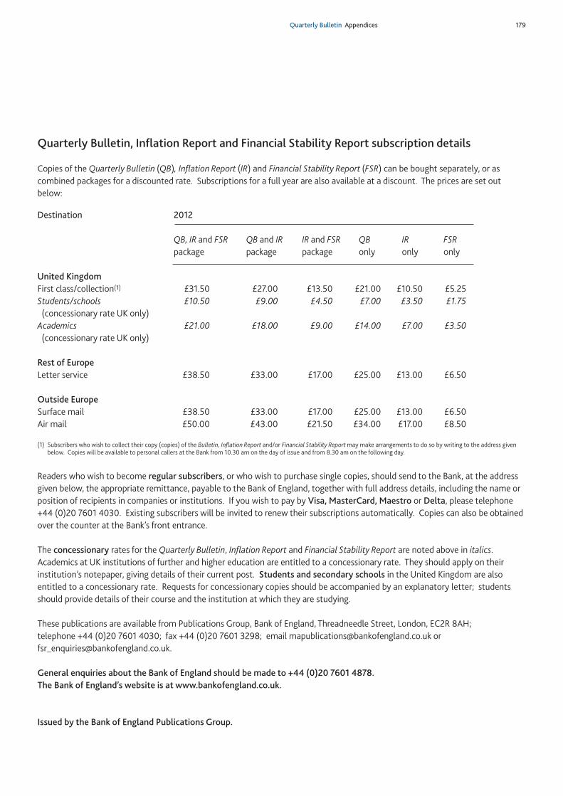
Quarterly Bulletin Appendices 179
Quarterly Bulletin, Inflation Report and Financial Stability Report subscription details
Copies of the Quarterly Bulletin (QB), Inflation Report (IR) and Financial Stability Report (FSR) can be bought separately, or ascombined packages for a discounted rate. Subscriptions for a full year are also available at a discount. The prices are set outbelow:
Destination 2012
QB, IR and FSR QB and IR IR and FSR QB IR FSRpackage package package only only only
United KingdomFirst class/collection(1) £31.50 £27.00 £13.50 £21.00 £10.50 £5.25Students/schools £10.50 £9.00 £4.50 £7.00 £3.50 £1.75(concessionary rate UK only)
Academics £21.00 £18.00 £9.00 £14.00 £7.00 £3.50(concessionary rate UK only)
Rest of EuropeLetter service £38.50 £33.00 £17.00 £25.00 £13.00 £6.50
Outside EuropeSurface mail £38.50 £33.00 £17.00 £25.00 £13.00 £6.50Air mail £50.00 £43.00 £21.50 £34.00 £17.00 £8.50
(1) Subscribers who wish to collect their copy (copies) of the Bulletin, Inflation Report and/or Financial Stability Report may make arrangements to do so by writing to the address givenbelow. Copies will be available to personal callers at the Bank from 10.30 am on the day of issue and from 8.30 am on the following day.
Readers who wish to become regular subscribers, or who wish to purchase single copies, should send to the Bank, at the addressgiven below, the appropriate remittance, payable to the Bank of England, together with full address details, including the name orposition of recipients in companies or institutions. If you wish to pay by Visa, MasterCard, Maestro or Delta, please telephone +44 (0)20 7601 4030. Existing subscribers will be invited to renew their subscriptions automatically. Copies can also be obtainedover the counter at the Bank’s front entrance.
The concessionary rates for the Quarterly Bulletin, Inflation Report and Financial Stability Report are noted above in italics.Academics at UK institutions of further and higher education are entitled to a concessionary rate. They should apply on theirinstitution’s notepaper, giving details of their current post. Students and secondary schools in the United Kingdom are alsoentitled to a concessionary rate. Requests for concessionary copies should be accompanied by an explanatory letter; studentsshould provide details of their course and the institution at which they are studying.
These publications are available from Publications Group, Bank of England, Threadneedle Street, London, EC2R 8AH; telephone +44 (0)20 7601 4030; fax +44 (0)20 7601 3298; email [email protected] [email protected].
General enquiries about the Bank of England should be made to +44 (0)20 7601 4878.The Bank of England’s website is at www.bankofengland.co.uk.
Issued by the Bank of England Publications Group.

© Bank of England 2012ISSN 0005-5166Printed by Park Communications Limited