Embed Size (px)
DESCRIPTION
The Quarterly Bulletin explores topics on monetary and financial stability and includes regular commentary on market developments and UK monetary policy operations. Some articles present analysis on current economic and financial issues, and policy implications. Other articles enhance the Bank’s public accountability by explaining the institutional structure of the Bank and the various policy instruments that are used to meet its objectives.
Citation preview
Quarterly Bulletin2015 Q2 | Volume 55 No. 2

Quarterly Bulletin2015 Q2 | Volume 55 No. 2
Topical articles
Mapping the UK financial system 114Box The subsectors of the financial system 122
Banking sector interconnectedness: what is it, how can we measure it and why does it matter? 130
The prudential regulation of insurers under Solvency II 139Box Transitioning to a ‘going-concern’ regime 144
A bank within a bank: how a commercial bank’s treasury function affects the interest rates set for loans and deposits 153Box Impact of economic and regulatory developments on FTP 159
Do inflation expectations currently pose a risk to inflation? 165Box What do financial market measures of inflation expectations tell us? 172Box Public attitudes to monetary policy and satisfaction with the Bank 179
Innovations in the Bank’s provision of liquidity insurance via Indexed Long-Term Repo (ILTR) operations 181
Recent economic and financial developments
Markets and operations 190
Report
A review of the work of the London Foreign Exchange Joint Standing Committee in 2014 198
Summaries of working papers
Summaries of recent Bank of England working papers 204– Can a data-rich environment help identify the sources of model misspecification? 204– Forecasting with VAR models: fat tails and stochastic volatility 205– Banks are not intermediaries of loanable funds — and why this matters 206
Appendices
Contents of recent Quarterly Bulletins 208
Bank of England publications 210
Contents

The contents page, with links to the articles in PDF, is available atwww.bankofengland.co.uk/publications/Pages/quarterlybulletin/default.aspx
Author of articles can be contacted [email protected]
Except where otherwise stated, the source of the data used in charts and tables is the Bank of England or the Office for National Statistics (ONS). All data, apart from financialmarkets data, are seasonally adjusted.
Research work published by the Bank is intended to contribute to debate, and does notnecessarily reflect the views of the Bank or members of the MPC, FPC or the PRA Board.

Topical articles
Quarterly Bulletin Topical articles 113
114 Quarterly Bulletin 2015 Q2
• The United Kingdom’s financial system is large and has grown rapidly in recent decades.Understanding its structure is an important starting point for a wide range of policy questions.
• One way into this is through the balance sheets of financial firms. This article paints a picture ofthe financial system by exploring those balance sheets, first using data currently available andthen looking ahead to new avenues of research that should further improve our understanding.
Mapping the UK financial system
By Oliver Burrows and Katie Low of the Bank’s Macro-financial Risks Division and Fergus Cumming of the Bank’sMonetary Assessment and Strategy Division.(1)
(1) The authors would like to thank David Matthews (ONS) and Iren Levina for their help in producing this article.
Overview
£220bnGeneral
insurance companies
£270bnFinance
companies
£400bnBank of England
£320bnSecuritisation
SPVs
£250bnUK other
banks
£160bnCentral
counterparties
£90bnExchange-traded
funds
£90bnInvestment
trusts
£90bnPrivateequity
Otherunauthorised
funds
Banks Non-banks
Liabilities
Assets
Liabilities
Assets
£3,570bn
Major UK internationalbanks
£1,160bn
Major UK domestic banks
£460bn
RoWotherbanks
£1,730bn
Rest of the world (RoW)investment banks
£1,430bn
Pension funds
£1,610bn
Life insurancecompanies
£700bn
Unit trusts
£670bn
Hedge funds
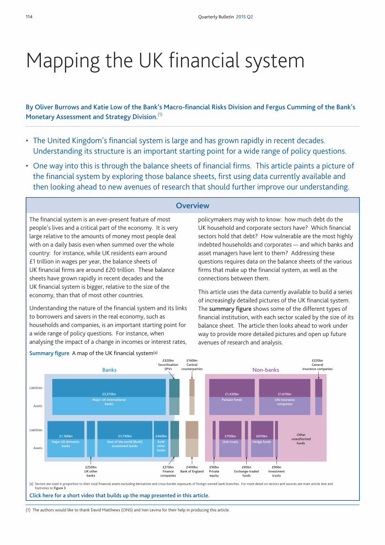
Summary figure A map of the UK financial system(a)
The financial system is an ever-present feature of mostpeople’s lives and a critical part of the economy. It is verylarge relative to the amounts of money most people dealwith on a daily basis even when summed over the wholecountry: for instance, while UK residents earn around£1 trillion in wages per year, the balance sheets ofUK financial firms are around £20 trillion. These balancesheets have grown rapidly in recent decades and theUK financial system is bigger, relative to the size of theeconomy, than that of most other countries.
Understanding the nature of the financial system and its linksto borrowers and savers in the real economy, such ashouseholds and companies, is an important starting point fora wide range of policy questions. For instance, whenanalysing the impact of a change in incomes or interest rates,
policymakers may wish to know: how much debt do theUK household and corporate sectors have? Which financialsectors hold that debt? How vulnerable are the most highlyindebted households and corporates — and which banks andasset managers have lent to them? Addressing thesequestions requires data on the balance sheets of the variousfirms that make up the financial system, as well as theconnections between them.
This article uses the data currently available to build a seriesof increasingly detailed pictures of the UK financial system.The summary figure shows some of the different types offinancial institution, with each sector scaled by the size of itsbalance sheet. The article then looks ahead to work underway to provide more detailed pictures and open up futureavenues of research and analysis.
(a) Sectors are sized in proportion to their total financial assets excluding derivatives and cross-border exposures of foreign-owned bank branches. For more detail on sectors and sources see main article text andfootnotes to Figure 3.
Click here for a short video that builds up the map presented in this article.
Topical articles Mapping the UK financial system 115
The financial system is an ever-present feature of mostpeople’s lives and a critical part of the economy. Financialinstitutions are important for the provision of financialservices. They facilitate the wage payments companies maketo staff and the transactions households make when they usecredit and debit cards to buy goods and services; provide loansto households and companies to allow some to consume andinvest today, while managing savings for tomorrow on behalfof others; and provide insurance against all sorts of adverseoutcomes, from ships sinking to pets needing medical care.
This article paints a picture of the financial system by exploringthe balance sheets of firms in the financial sector. A detailedpicture of UK balance sheets is a starting point for answering awide range of policy questions. For instance, when analysingthe impact of a change in income or interest rates,policymakers may wish to know: how much debt do theUK household and corporate sectors have? Which financialsectors hold that debt? Addressing these questions requiresdata on the balance sheets of the various sectors that togethermake up the financial system, as well as the connectionsbetween those sectors. Going further, policymakers might ask:how vulnerable are the most highly indebted households andcorporates? And which banks and asset managers have lent tothem? These questions require data on firm-level balancesheets and firm-level interconnections. This article uses thedata currently available to build a series of increasinglydetailed pictures of the UK financial system. It then looksahead to work under way to provide more detailed picturesand open up future avenues of research and analysis.
The first section of this article briefly sets the scene bydescribing how the sizes of financial systems compare acrosscountries and across time. The second section describes thehigh-level functions of a financial sector and presents a scaled‘map’ of the financial balance sheets of the UK economy, splitinto various financial and non-financial sectors. The thirdsection illustrates the distribution of financial assets withinsectors, highlighting the need to understand where features ofa sector are common across all firms versus instances in whichthe differences within sectors are as important as thesimilarities. The final section outlines ongoing work betweenthe Bank and the Office for National Statistics (ONS) toexpand the standard National Accounts to encompass moredetail within the financial sector, more availability ofanonymised microdata and collection of ‘who-to-whom’ datato allow better mapping of the connections between sectors.A short video builds up the map of the financial systempresented in this article.(1)
Setting the scene: how big is the UK financialsystem?
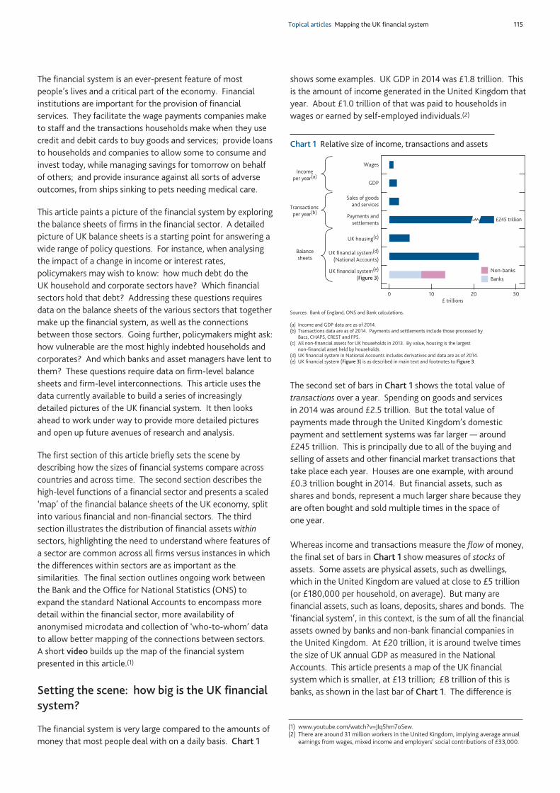
The financial system is very large compared to the amounts ofmoney that most people deal with on a daily basis. Chart 1
shows some examples. UK GDP in 2014 was £1.8 trillion. Thisis the amount of income generated in the United Kingdom thatyear. About £1.0 trillion of that was paid to households inwages or earned by self-employed individuals.(2)
The second set of bars in Chart 1 shows the total value oftransactions over a year. Spending on goods and servicesin 2014 was around £2.5 trillion. But the total value ofpayments made through the United Kingdom’s domesticpayment and settlement systems was far larger — around£245 trillion. This is principally due to all of the buying andselling of assets and other financial market transactions thattake place each year. Houses are one example, with around£0.3 trillion bought in 2014. But financial assets, such asshares and bonds, represent a much larger share because theyare often bought and sold multiple times in the space ofone year.
Whereas income and transactions measure the flow of money,the final set of bars in Chart 1 show measures of stocks ofassets. Some assets are physical assets, such as dwellings,which in the United Kingdom are valued at close to £5 trillion(or £180,000 per household, on average). But many arefinancial assets, such as loans, deposits, shares and bonds. The‘financial system’, in this context, is the sum of all the financialassets owned by banks and non-bank financial companies inthe United Kingdom. At £20 trillion, it is around twelve timesthe size of UK annual GDP as measured in the NationalAccounts. This article presents a map of the UK financialsystem which is smaller, at £13 trillion; £8 trillion of this isbanks, as shown in the last bar of Chart 1. The difference is
(1) www.youtube.com/watch?v=Jlq5hm7oSew.(2) There are around 31 million workers in the United Kingdom, implying average annual
earnings from wages, mixed income and employers’ social contributions of £33,000.
UK financial system(e)
(Figure 3)
UK financial system(d)
(National Accounts)
UK housing(c)
Payments andsettlements
Sales of goodsand services
GDP
WagesIncome
per year(a)
Transactions per year(b)
Balancesheets
0 10 20 30£ trillions
£245 trillion
Non-banks
Banks
Sources: Bank of England, ONS and Bank calculations.
(a) Income and GDP data are as of 2014.(b) Transactions data are as of 2014. Payments and settlements include those processed by
Bacs, CHAPS, CREST and FPS.(c) All non-financial assets for UK households in 2013. By value, housing is the largest
non-financial asset held by households.(d) UK financial system in National Accounts includes derivatives and data are as of 2014.(e) UK financial system (Figure 3) is as described in main text and footnotes to Figure 3.
Chart 1 Relative size of income, transactions and assets
116 Quarterly Bulletin 2015 Q2
due to a number of design choices, principally the exclusion ofderivatives, described later in the article.
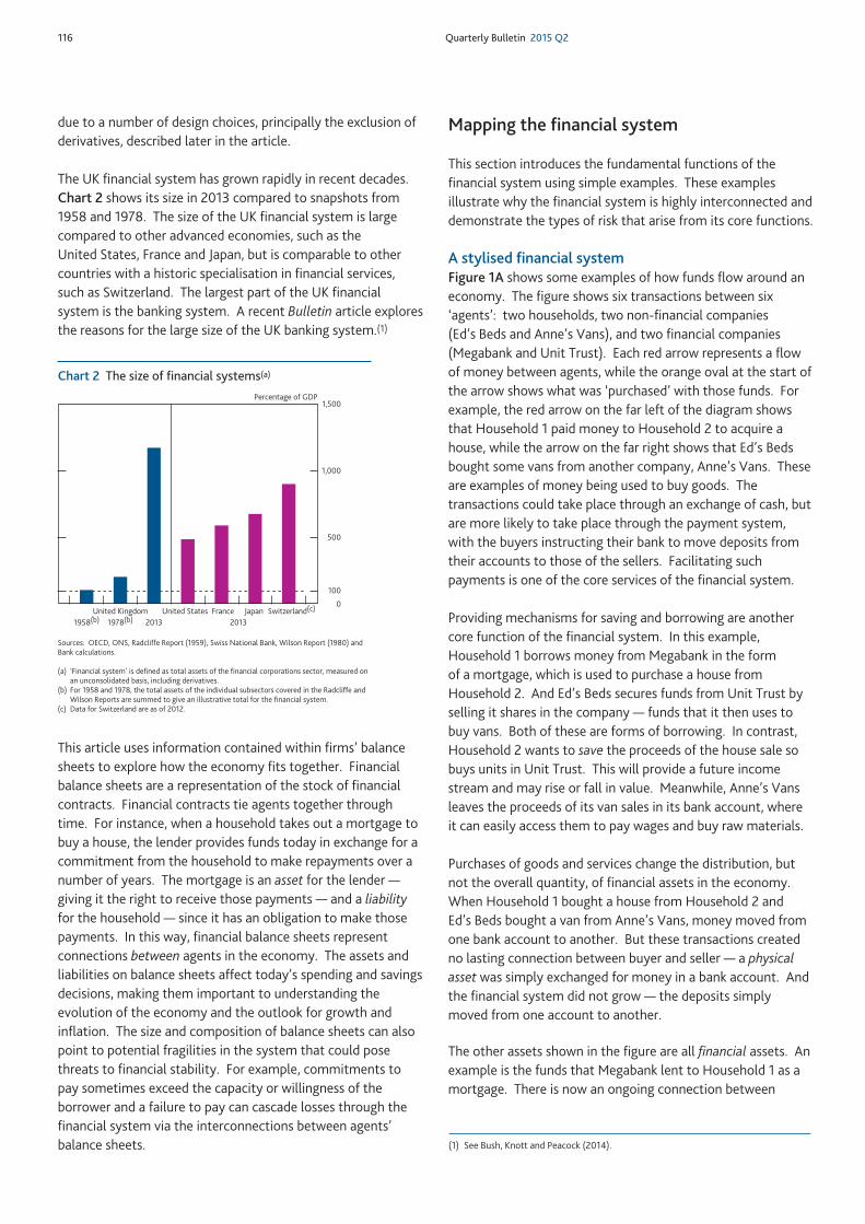
The UK financial system has grown rapidly in recent decades.Chart 2 shows its size in 2013 compared to snapshots from1958 and 1978. The size of the UK financial system is largecompared to other advanced economies, such as theUnited States, France and Japan, but is comparable to othercountries with a historic specialisation in financial services,such as Switzerland. The largest part of the UK financialsystem is the banking system. A recent Bulletin article exploresthe reasons for the large size of the UK banking system.(1)
This article uses information contained within firms’ balancesheets to explore how the economy fits together. Financialbalance sheets are a representation of the stock of financialcontracts. Financial contracts tie agents together throughtime. For instance, when a household takes out a mortgage tobuy a house, the lender provides funds today in exchange for acommitment from the household to make repayments over anumber of years. The mortgage is an asset for the lender —giving it the right to receive those payments — and a liabilityfor the household — since it has an obligation to make thosepayments. In this way, financial balance sheets representconnections between agents in the economy. The assets andliabilities on balance sheets affect today’s spending and savingsdecisions, making them important to understanding theevolution of the economy and the outlook for growth andinflation. The size and composition of balance sheets can alsopoint to potential fragilities in the system that could posethreats to financial stability. For example, commitments topay sometimes exceed the capacity or willingness of theborrower and a failure to pay can cascade losses through thefinancial system via the interconnections between agents’balance sheets.
Mapping the financial system
This section introduces the fundamental functions of thefinancial system using simple examples. These examplesillustrate why the financial system is highly interconnected anddemonstrate the types of risk that arise from its core functions.
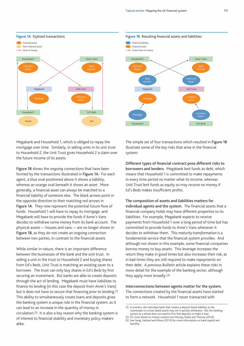
A stylised financial system Figure 1A shows some examples of how funds flow around aneconomy. The figure shows six transactions between six‘agents’: two households, two non-financial companies(Ed’s Beds and Anne’s Vans), and two financial companies(Megabank and Unit Trust). Each red arrow represents a flowof money between agents, while the orange oval at the start ofthe arrow shows what was ‘purchased’ with those funds. Forexample, the red arrow on the far left of the diagram showsthat Household 1 paid money to Household 2 to acquire ahouse, while the arrow on the far right shows that Ed’s Bedsbought some vans from another company, Anne’s Vans. Theseare examples of money being used to buy goods. Thetransactions could take place through an exchange of cash, butare more likely to take place through the payment system,with the buyers instructing their bank to move deposits fromtheir accounts to those of the sellers. Facilitating suchpayments is one of the core services of the financial system.
Providing mechanisms for saving and borrowing are anothercore function of the financial system. In this example,Household 1 borrows money from Megabank in the formof a mortgage, which is used to purchase a house fromHousehold 2. And Ed’s Beds secures funds from Unit Trust byselling it shares in the company — funds that it then uses tobuy vans. Both of these are forms of borrowing. In contrast,Household 2 wants to save the proceeds of the house sale sobuys units in Unit Trust. This will provide a future incomestream and may rise or fall in value. Meanwhile, Anne’s Vansleaves the proceeds of its van sales in its bank account, whereit can easily access them to pay wages and buy raw materials.
Purchases of goods and services change the distribution, butnot the overall quantity, of financial assets in the economy.When Household 1 bought a house from Household 2 andEd’s Beds bought a van from Anne’s Vans, money moved fromone bank account to another. But these transactions createdno lasting connection between buyer and seller — a physicalasset was simply exchanged for money in a bank account. Andthe financial system did not grow — the deposits simplymoved from one account to another.
The other assets shown in the figure are all financial assets. Anexample is the funds that Megabank lent to Household 1 as amortgage. There is now an ongoing connection between
0
500
1,000
1,500
Switzerland(c)JapanFranceUnited States20131978(b)1958(b) 2013
Percentage of GDP
100
United Kingdom
Sources: OECD, ONS, Radcliffe Report (1959), Swiss National Bank, Wilson Report (1980) andBank calculations.
(a) ‘Financial system’ is defined as total assets of the financial corporations sector, measured onan unconsolidated basis, including derivatives.
(b) For 1958 and 1978, the total assets of the individual subsectors covered in the Radcliffe andWilson Reports are summed to give an illustrative total for the financial system.
(c) Data for Switzerland are as of 2012.
Chart 2 The size of financial systems(a)
(1) See Bush, Knott and Peacock (2014).
Topical articles Mapping the UK financial system 117
Megabank and Household 1, which is obliged to repay themortgage over time. Similarly, in selling units in its unit trustto Household 2, the Unit Trust gives Household 2 a claim overthe future income of its assets.
Figure 1B shows the ongoing connections that have beenformed by the transactions illustrated in Figure 1A. For eachagent, a blue oval positioned above it shows a liability,whereas an orange oval beneath it shows an asset. Moregenerally, a financial asset can always be matched to afinancial liability of someone else. The black arrows point inthe opposite direction to their matching red arrows inFigure 1A. They now represent the potential future flow offunds: Household 1 will have to repay its mortgage, andMegabank will have to provide the funds if Anne’s Vansdecides to withdraw some money from its bank account. Thephysical assets — houses and vans — are no longer shown inFigure 1B, as they do not create an ongoing connectionbetween two parties, in contrast to the financial assets.
While similar in nature, there is an important differencebetween the businesses of the bank and the unit trust. Inselling a unit in the trust to Household 2 and buying sharesfrom Ed’s Beds, Unit Trust is matching an existing saver to aborrower. The trust can only buy shares in Ed’s Beds by firstsecuring an investment. But banks are able to create depositsthrough the act of lending. Megabank must have liabilities tofinance its lending (in this case the deposit from Anne’s Vans)but it does not have to secure that financing prior to lending.(1)
This ability to simultaneously create loans and deposits givesthe banking system a unique role in the financial system, as itcan lead to an increase in the quantity of money incirculation.(2) It is also a key reason why the banking system isof interest to financial stability and monetary policy makersalike.
The simple set of four transactions which resulted in Figure 1Billustrate some of the key risks that arise in the financialsystem:
Different types of financial contract pose different risks toborrowers and lenders. Megabank lent funds as debt, whichmeans that Household 1 is committed to make repaymentsin every time period no matter what its income, whereasUnit Trust lent funds as equity so may receive no money ifEd’s Beds makes insufficient profits.
The composition of assets and liabilities matters forindividual agents and the system. The financial assets that afinancial company holds may have different properties to itsliabilities. For example, Megabank expects to receivepayments from Household 1 over a long period of time but hascommitted to provide funds to Anne’s Vans whenever itdecides to withdraw them. This maturity transformation is afundamental service that the financial system provides. Andalthough not shown in this example, some financial companiesborrow money to buy assets. This leverage increases thereturn they make in good times but also increases their risk, asin bad times they are still required to make repayments ontheir debt. A previous Bulletin article explains these risks inmore detail for the example of the banking sector, althoughthey apply more broadly.(3)
Interconnections between agents matter for the system.The connections created by the financial assets have startedto form a network. Household 1 never transacted with
Financial asset
Non-financial asset
Flow of money
Household 1
House
Household 2
Unit trustshares
Megabank
Mortgage
Unit Trust
Companyshares
Ed’s Beds
Van
Anne’s Vans
Bankaccount
Figure 1A Stylised transactions
Financial liability
Financial asset
Future flow of money
Unit trustshares
Companyshares
Unit trustshares
Bankaccount
Household 1
Household 2
Megabank
Mortgage
Unit Trust
Ed’s Beds
Anne’s Vans
Mortgage Companyshares
Bankaccount
Figure 1B Resulting financial assets and liabilities
(1) In practice, the individual bank that creates a deposit (bank liability) as thecounterpart to a loan (bank asset) may see it quickly withdrawn. But the bankingsystem as a whole does not need to first find deposits to make a loan.
(2) For more detail on money creation see McLeay, Radia and Thomas (2014).(3) See Farag, Harland and Nixon (2013) for more information on bank capital and
liquidity.
118 Quarterly Bulletin 2015 Q2
Anne’s Vans but both are connected to Megabank so that,in theory, the safety of Anne’s Vans’ asset is connected toHousehold 1’s ability to repay Megabank.(1) As moreconnections are added, agents in the economy become evermore interconnected without ever dealing directly with eachother. An accompanying article in this edition of the Bulletindiscusses interconnectedness in more detail, focusing on thebanking sector.(2)
Mapping out the stocks of financial assets and liabilitiestherefore helps to answer the questions about risks andvulnerabilities that were posed in the introduction.
Drawing the map to scaleFigure 1B showed four stylised contracts. In the rest of thisarticle, the figure will be expanded to cover all of the financialassets and liabilities in the UK economy. They will be shownto scale to illustrate how large different parts of the financialsystem are. To do this, it will be necessary to simplify thefigure in a number of ways. First, as more agents are added,they will be grouped by type. For example, instead of showingeach of the 27 million households in the United Kingdom, themap will show one aggregated household sector, comprisingthe assets and liabilities of all UK households. Second,Figure 1B showed examples in which each agent in the realeconomy (the households and companies) had either financialassets or liabilities. In reality, many have both — but thefigure will continue to be drawn with the financial assets ofthose in the real economy shown at the top and their liabilitiesshown at the bottom of the figure. Finally, the black arrowswill not be drawn in. The final section of this article considersan example of what the map might look like if thesesimplifying choices were not made. It also describes ongoingwork between the ONS and Bank of England to collectsufficient detailed data to draw such a map.
Since 1987, the ONS has published data on the financialbalance sheets of the UK economy each year (within theNational Accounts, known as the ‘Blue Book’).(3) The ONSorganises the economy into seven sectors: non-financialcorporations (NFCs); government;(4) households;(5) monetaryfinancial institutions (MFIs); insurance companies and pensionfunds (ICPFs); other financial institutions (OFIs); and the restof the world (RoW).(6) Assets and liabilities for RoW areincluded where one party to the contract is a non-residententity. All such non-resident entities are collected togetherinto a single balance sheet (for example, a UK bank lending toa company overseas is counted as a RoW liability, while anoverseas bank lending to a UK company is counted as a RoWasset).(7) Returning to the agents in Figure 1B, Megabankwould be classified within MFIs while Unit Trust would sitwithin OFIs.
Figure 2 shows the scaled financial balance sheets of theUK economy using ONS data for 2014. Each sector is
represented by a pair of boxes with an area that is inproportion to its total financial assets and liabilities.(8) Thevalues of non-financial assets owned by the real economy,such as houses or vans, are shown as additional boxes at thetop of the figure. Substantial amounts of wealth are held innon-financial assets: the stock of UK housing (the largestnon-financial asset owned by households) is worth about£5 trillion and NFCs own about £1.9 trillion of capital stock.
A map of the financial systemFigure 2 contains some useful information on the size andcomposition of the UK financial system. Moreover, becausethe data come from the National Accounts, the data in themap are consistent with the activity captured elsewhere inthose accounts, such as GDP, consumption and investment inphysical capital. For many questions in economics, this levelof detail is sufficient. But for some questions, including manythat relate to the Bank’s policy goals, more detail can berequired.
The Bank of England has committees charged withmaintaining monetary stability (the Monetary PolicyCommittee (MPC)) and financial stability (the Financial PolicyCommittee (FPC)). In addition, the Prudential RegulationAuthority (PRA) Board oversees the PRA’s role in promotingthe safety and soundness of firms it regulates, and protectingpolicyholders of insurance contracts. The informationrequired by all three bodies to meet their objectives is likely toextend beyond the data contained in the National Accounts.As an example, in looking for vulnerabilities in theUnited Kingdom’s external balance sheet that mightexacerbate the risks around the current account deficit, theDecember 2014 Financial Stability Report emphasised the needfor greater detail than is available in the National Accounts.This has been an active area of research recently.(9)
(1) In practice, for individuals and smaller businesses, deposits in the United Kingdom ofup to £85,000 are protected by the Financial Services Compensation Scheme.
(2) See Liu, Quiet and Roth (2015) in this edition of the Bulletin.(3) National Accounts have been published each year since 1952 but balance sheets were
not included until later. From 1978 the Central Statistical Office started to produceregular information on UK financial balance sheets in its publications. Sporadicattempts to estimate the stock of assets (financial and non-financial) started muchearlier, with the Domesday Book perhaps the best-known example. Piketty (2014)gives a brief history of economists’ attempts to measure national accounts includingstock information (see ‘National Accounts: an evolving social construct’, pages 55–59). Pozsar et al (2010) is a recent example of visually representing howparts of the financial system fit together.
(4) Includes central and local government.(5) This ONS sector also includes non-profit institutions serving households.(6) The current standards for ONS National Accounts are known as ESA 2010. NFCs are
also split into public and private (here meaning those owned by the state or not)though public NFCs are of negligible size in practice.
(7) In a closed economy, the total size of financial assets would be equal to the total sizeof financial liabilities. For an open economy, by including these ‘RoW’ assets andliabilities, the National Accounts maintain this identity: that total assets andliabilities are equal.
(8) Financial institutions typically do not have substantial non-financial assets so thatthey have financial assets of roughly the same size as their liabilities. Assets do notequal liabilities exactly, however, due to the difference between the book value ofequity and the market value of equity, for example.
(9) See Box 2 on pages 29–31 of the December 2014 Financial Stability Report;www.bankofengland.co.uk/publications/Documents/fsr/2014/fsrfull1412.pdf.

Topical articles Mapping the UK financial system 119
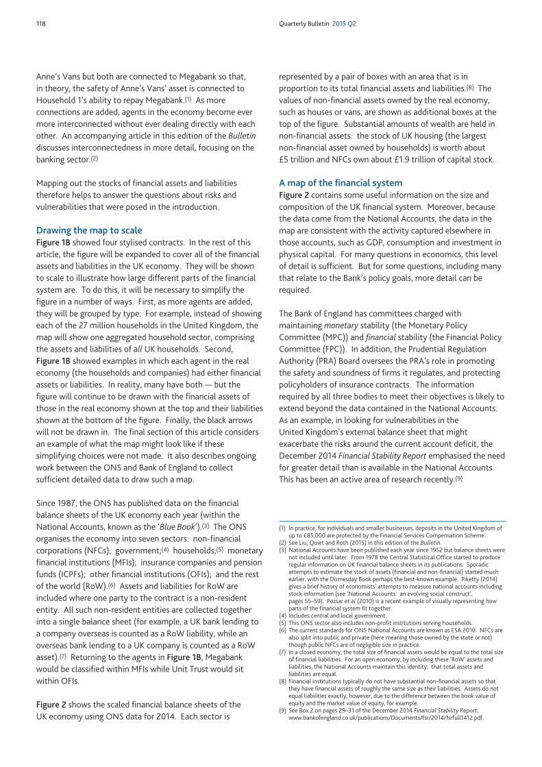
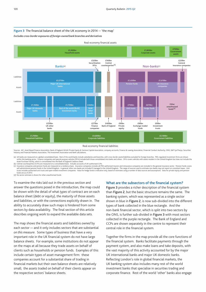
To this end, Figure 3 presents a ‘map’ of the financial system.The RoW sector and real-economy physical assets have beenstripped out. The length of each box is now directlyproportional to the size of the sector’s assets or liabilities.Sectors within the financial system are shown at double heightas the map shows both their assets and liabilities. Thenon-bank financial sector has been separated into a number ofmeaningfully distinct subsectors such as pension funds, hedgefunds and life insurance companies. The map is drawn at alevel of detail at which it is reasonable to compare institutionswithin each financial sector and to aggregate their balancesheets to give a single representative balance sheet for thatsector. For instance, it makes sense to think of all unit trustsas having some features in common, whereas in the NationalAccounts OFI sector, unit trusts are aggregated up alongsidecentral counterparties, which perform a completely separatefunction. Similarly, the MFI sector has been split into differenttypes of banking business, paying particular attention towhether they are UK or foreign-owned, which is an importantdistinction in particular for many regulatory and financialstability issues.
Figure 3 includes some important design choices, to helpfocus on the flow of funds within the UK financial system.First, it excludes derivatives. Derivatives are important for theprovision of some services, are a significant proportion ofsome firms’ balance sheets and lead to importantinterconnections within the financial system, particularlybetween banks. But their contingent nature, together with thepractice of a small number of financial firms holding verylarge, offsetting positions that cancel out to small netpositions, means that it is not sensible to directly compare
their size to other financial assets. Second, it excludes theforeign assets and liabilities of foreign branches. Thissignificantly reduces the size of the ‘RoW other banks’ sector.While important for those banks and some policy purposes, itis useful to remove these assets and liabilities here to focus onthe United Kingdom.
A further way in which Figure 3 differs to Figure 2 is that thebanking system is illustrated on a consolidated basis, capturingthe global activity of UK-based institutions.(1) This is differentto the residency basis of the National Accounts but can bemore useful for answering some questions related to financialstability.(2) But this choice comes at a cost — the accounts areno longer consistent with other measures of UK activity. Italso means that for a small proportion of assets (liabilities),the corresponding liability (asset) is no longer shown.
Figure 3 is not the only way to dissect the financial system butit is one that makes sense based on current structures andanalysis of the financial system. Other decompositions couldbe drawn as the financial structure of the economy changesand more information becomes available. The initial attemptsto collect information on the UK financial system as part ofthe Radcliffe Report (1959), and later the Wilson Report(1980), serve as a reminder that our data and analysis need toevolve in line with the financial landscape.(3)
£7,800 billionRest of the world assets(c)
£4,800 billionHousehold non-financial assets(b)
£1,900 billionCorporate non-financial assets(b)
£5,900 billionHousehold assets
£1,800 billionCorporate assets
£1,700 billionHousehold liabilities
£4,600 billionCorporate liabilities
£2,100 billionGovernment liabilities
£7,200 billionMFI liabilities
£7,400 billionMFI assets
£3,800 billionICPF liabilities
£4,500 billionOFI liabilities
£3,700 billionICPF assets
£4,000 billionOFI assets£7,400 billion
Rest of the world liabilities(c)
£970 billionGovernment
non-financial assets(b)
£700 billionGovernment
assets
Source: ONS.
(a) Figure shows financial assets excluding derivatives. MFI refers to monetary financial institutions, ICPF refers to insurance companies and pension funds and OFI refers to other financial institutions. Financial assets may not beequal to financial liabilities for individual companies, and hence sectors. This is due primarily to excluding non-financial assets, using market values for equity and the exclusion of derivatives. The coloured dashed lines indicatethe balancing value for sectors.
(b) Values for non-financial assets are as of 2013. Non-financial assets of financial sectors are not shown in the figure.(c) Rest of the world assets and liabilities are included where one party to a contract is not a resident in the United Kingdom. See main text for more details.
Figure 2 The balance sheet of the UK economy in 2014 — using National Accounts data(a)
(1) A further difference is that large investment firms that are regulated by the PRA havebeen grouped with banks in Figure 3 whereas they would fall under OFIs in Figure 2.
(2) The National Accounts seek to capture the economic activity of agents resident in theUnited Kingdom, regardless of the nationality of their ultimate owner. For example,this leads them to capture the balance sheets of foreign-owned, UK-resident bankbranches; but not UK-owned, foreign-resident bank branches.
(3) See Davies et al (2010) for discussion on the evolution of the UK banking system.
120 Quarterly Bulletin 2015 Q2
To examine the risks laid out in the previous section andanswer the questions posed in the introduction, the map couldbe shown with the detail of what types of contract are on eachbalance sheet (debt or equity), the maturity of those assetsand liabilities, or with the connections explicitly drawn in. Theability to accurately draw such maps is hindered from somesectors by data availability. The final section of this articledescribes ongoing work to expand the available data sets.
The map shows the financial assets and liabilities owned byeach sector — and it only includes sectors that are substantialon this measure. Some types of business that have a veryimportant role in the UK financial system do not have largebalance sheets. For example, some institutions do not appearon the maps at all because they trade assets on behalf ofclients such as households or pension funds. Examples of thisinclude certain types of asset management firm: thesecompanies account for a substantial share of trading infinancial markets but their own balance sheets are relativelysmall; the assets traded on behalf of their clients appear onthe respective sectors’ balance sheets.
What are the subsectors of the financial system?Figure 3 provides a richer description of the financial systemthan Figure 2, but the basic structure remains the same. Thebanking system, which was represented as a single sectorshown in blue in Figure 2, is now sub-divided into the differenttypes of bank collected in the blue rectangle. And thenon-bank financial sector, which is split into two sectors bythe ONS, is further sub-divided in Figure 3 with most sectorscollected in the purple rectangle. The Bank of England andCCPs are shown separately in the centre to represent theircentral role in the financial system.
Together the firms in the map provide all the core functions ofthe financial system. Banks facilitate payments through thepayment system, and also make loans and take deposits, withthe vast majority of this activity accounted for by the majorUK international banks and major UK domestic banks.Reflecting London’s role in global financial markets, theUK banking system also includes many rest of the worldinvestment banks that specialise in securities trading andcorporate finance. Rest of the world ‘other’ banks also engage
£220bnGeneral
insurance companies
£270bnFinance
companies
£1,800bnCorporate assets
£700bnGovernment
assets
£400bnBank of England
£320bnSecuritisation
SPVs
£1,700bnHousehold liabilities
£4,600bnCorporate liabilities
£2,100bnGovernment liabilities
£250bnUK other
banks
£160bnCentral
counterparties(b)
£90bnExchange-traded
funds
£90bnInvestment
trusts
£90bnPrivateequity
Otherunauthorised
funds(d)
Real-economy financial assets
Real-economy financial liabilities
Banks(a) Non-banks(c)
Liabilities
Assets
Liabilities
Assets
£5,900bnHousehold assets
£3,570bn
Major UK internationalbanks
£1,160bn
Major UK domestic banks
£460bn
RoWotherbanks
£1,730bn
Rest of the world (RoW)investment banks
£1,430bn
Pension funds
£1,610bn
Life insurancecompanies
£700bn
Unit trusts
£670bn
Hedge funds
Excludes cross-border exposures of foreign-owned bank branches and derivatives
Sources: AIC, Asset Based Finance Association, Bank of England, British Private Equity & Venture Capital Association, company accounts, Finance & Leasing Association, Financial Conduct Authority, ONS, S&P SynThesys, SecuritiesIndustry and Financial Markets Association, The Investment Association and Bank calculations.
(a) UK banks are measured on a global consolidated basis. Rest of the world banks include subsidiaries and branches, with cross-border assets/liabilities excluded for foreign branches. PRA-regulated investment firms are shownwithin the banking sector. Finance companies and special purpose vehicles (SPVs) include both those consolidated into banks and others. SPVs covers vehicles with assets resident in the United Kingdom but does not include theAsset Purchase Facility, which is consolidated into the Bank of England’s balance sheet.
(b) Central counterparties (CCPs) are measured on a consolidated basis. Includes accounts of UK-authorised CCPs.(c) Insurance companies and pension funds are measured on a residency basis. Insurance companies includes all PRA-authorised insurers and reinsurance companies are included in the general insurance sector. Pension funds covers
self-administered pension funds in the United Kingdom. In general, other non-banks are included if managed in the United Kingdom. The range of sources used to estimate non-banks may not report on consistent bases. Unittrusts includes authorised unit trusts and open-ended investment companies. Value for hedge funds is indicative only, based on estimates using a number of data sources and assumptions. Data for private equity and pensionfunds are as of 2013.
(d) No sector estimate is shown for other unauthorised funds.
Figure 3 The financial balance sheet of the UK economy in 2014 — ‘the map’
Topical articles Mapping the UK financial system 121
in these kinds of activities but tend to interact less with theUK real economy.
Turning to non-bank financial institutions, fund managers offerinvestment products and services for savers, on whose behalfthey lend money in the form of debt or equity to borrowers.Unit trusts are one example, but they sit alongside pensionfunds, hedge funds and other collective investment schemes.Finally, the map shows insurers: life insurance companiesprovide long-term savings products, typically involvingprovision for retirement. General insurers, meanwhile, provideinsurance against particular events, such as a car being stolenor a pet needing veterinary care. The box on pages 122–24explains all of the different types of financial institution thatfeature in the map in more detail.
How representative are the aggregatesectors?
Analysing sectors using disaggregate analysisIn Figure 3, institutions have been assigned to sectorsdepending on the defining characteristics of their business.Understanding the characteristics of each of these sectors andtheir aggregate financial balance sheet is important forassessing both the risks they face and the risks they pose tothe rest of the financial system. But availability of underlyingindividual entity data also allows analysis of whether sectoraggregates give a good approximation of a representativebalance sheet of a representative company or the total risk ofthe sector. There could, for example, be a set of vulnerable
institutions or individuals that pose a broader risk to financialstability than can be seen from the aggregate data for thatsector alone.
For this reason, more detailed analyses often concern howmetrics are distributed across a sector. For example, theJune 2014 Financial Stability Report focused on the distributionof debt across households rather than aggregate indebtedness.The FPC was concerned that an increase in the number ofhighly indebted households could lead to an economy thatwould be more vulnerable in the face of shocks.
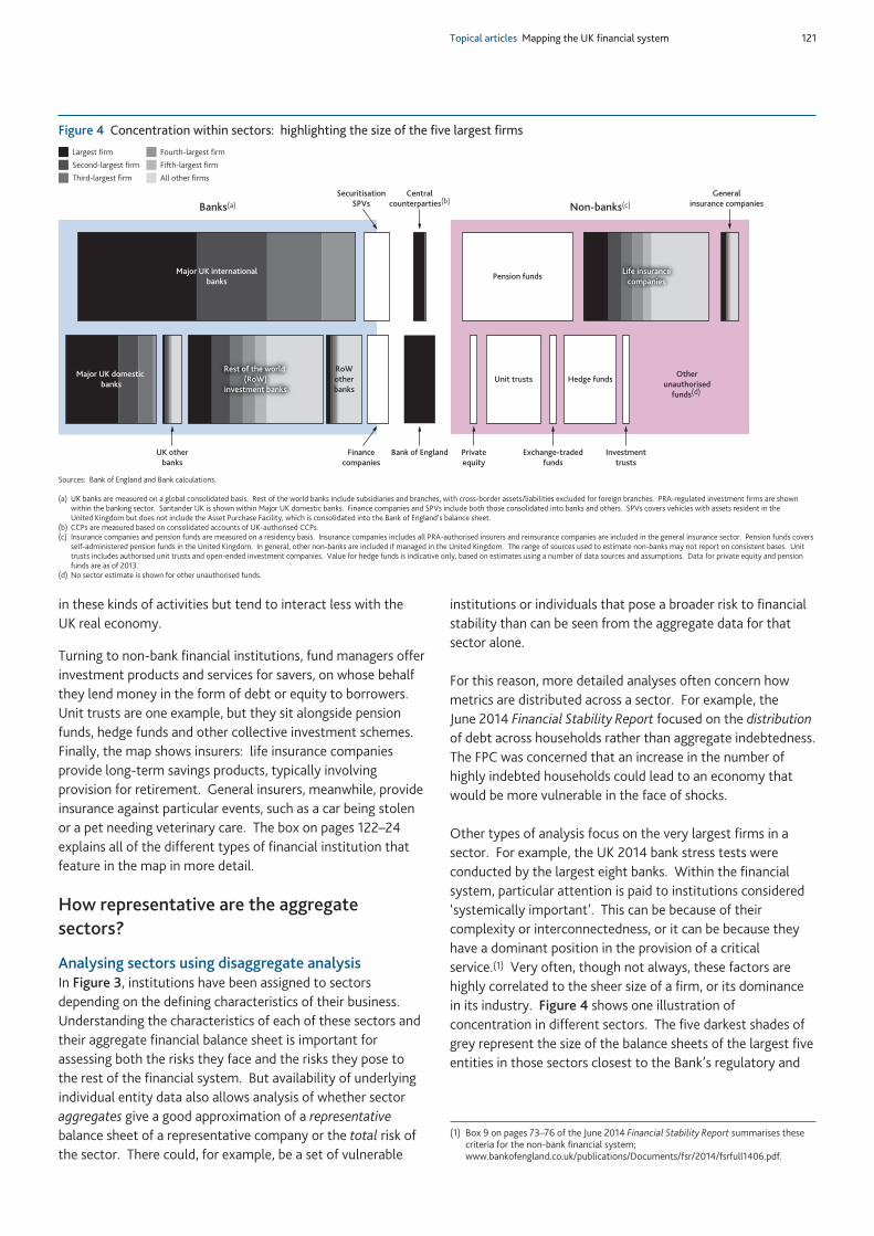
Other types of analysis focus on the very largest firms in asector. For example, the UK 2014 bank stress tests wereconducted by the largest eight banks. Within the financialsystem, particular attention is paid to institutions considered‘systemically important’. This can be because of theircomplexity or interconnectedness, or it can be because theyhave a dominant position in the provision of a criticalservice.(1) Very often, though not always, these factors arehighly correlated to the sheer size of a firm, or its dominancein its industry. Figure 4 shows one illustration ofconcentration in different sectors. The five darkest shades ofgrey represent the size of the balance sheets of the largest fiveentities in those sectors closest to the Bank’s regulatory and
(1) Box 9 on pages 73–76 of the June 2014 Financial Stability Report summarises thesecriteria for the non-bank financial system;www.bankofengland.co.uk/publications/Documents/fsr/2014/fsrfull1406.pdf.
Generalinsurance companies
Financecompanies
Major UK internationalbanks
Bank of England
Major UK domestic banks
RoWotherbanks
SecuritisationSPVs
UK otherbanks
Centralcounterparties(b)
Exchange-tradedfunds
Investmenttrusts
Privateequity
Pension funds
Unit trusts Hedge funds
Banks(a) Non-banks(c)
Largest firm
Second-largest firm
Third-largest firm
Fourth-largest firm
Fifth-largest firm
All other firms
Otherunauthorised
funds(d)
Rest of the world (RoW)
investment banks
Life insurancecompanies
Sources: Bank of England and Bank calculations.
(a) UK banks are measured on a global consolidated basis. Rest of the world banks include subsidiaries and branches, with cross-border assets/liabilities excluded for foreign branches. PRA-regulated investment firms are shownwithin the banking sector. Santander UK is shown within Major UK domestic banks. Finance companies and SPVs include both those consolidated into banks and others. SPVs covers vehicles with assets resident in theUnited Kingdom but does not include the Asset Purchase Facility, which is consolidated into the Bank of England’s balance sheet.
(b) CCPs are measured based on consolidated accounts of UK-authorised CCPs.(c) Insurance companies and pension funds are measured on a residency basis. Insurance companies includes all PRA-authorised insurers and reinsurance companies are included in the general insurance sector. Pension funds covers
self-administered pension funds in the United Kingdom. In general, other non-banks are included if managed in the United Kingdom. The range of sources used to estimate non-banks may not report on consistent bases. Unittrusts includes authorised unit trusts and open-ended investment companies. Value for hedge funds is indicative only, based on estimates using a number of data sources and assumptions. Data for private equity and pensionfunds are as of 2013.
(d) No sector estimate is shown for other unauthorised funds.
Figure 4 Concentration within sectors: highlighting the size of the five largest firms
122 Quarterly Bulletin 2015 Q2
The subsectors of the financial system
This box provides more detail on the different types offinancial institution shown in the map of the UK financialsystem (Figure 3). Some of these institutions are fairlycomplex, so for further details the box links to other sourcesof information.
Banks(1)Banks provide some of the core services of a financial system,including holding deposits, providing payment services andlending to households and companies. The UK banking sectoris large compared to other developed countries andparticularly international in nature: both in terms of the scaleof foreign bank activity in the United Kingdom and the scale ofthe international operations of UK-owned banks. A recentQuarterly Bulletin article explains that this is partly due toLondon’s history as a financial centre and considers theimplications of such a large banking sector for financialstability.(2)
Figure 3 separates the sector into different types of bank.The UK-owned banks are split into three groups. Theeight lenders in the United Kingdom that took part in the2014 stress-testing exercise make up the first two groups,distinguished by the extent of their overseas business: themajor UK international banks and the major UK domesticbanks.(3) All other UK-owned banks (both retail andinvestment banks) and building societies are in the groupUK other banks.(4)
The subsidiaries and branches of overseas banks are split intotwo groups. Investment banks operate in capital markets,either to help companies and governments raise funds, or tomanage risks for clients.(5) This sector includes PRA‘designated firms’ — institutions that do not accept depositsbut which are still prudentially regulated by the PRA. Otherbranches and subsidiaries of overseas banks operating in theUnited Kingdom are shown as RoW other banks. Manyinternational banks have branches operating in London, whichis an international financial centre, but actually do littlebusiness with UK clients. Because the focus here is on theUK financial system, the exposures to non-residents ofbranches operating in the United Kingdom have been excludedfrom this map. This is an important design decision. If theywere included, they would be substantially larger.
Semi-banking sectorsTwo types of institution are illustrated as sitting on the borderof banking: securitisation special purpose vehicles (SPVs) andfinance companies. They are illustrated in this way becausethey are often, though not always, owned by banks.
Like banks, finance companies lend money to the realeconomy. And many finance companies are owned by banks.But finance companies themselves are not banks as they donot use customer deposits to finance the loans they make.
One common way that finance companies and banks fundtheir lending activities is via the process of securitisation,explained in more detail in Balluck (2015). Securitisationinvolves selling a bundle of loans to a separate entity calledan SPV, which holds these loans as its assets. The SPV thenissues debt securities to outside investors, where the interestand principle payments are covered by the cash flows from theoriginal loans. In this way, the risk associated with the loanscan be transferred to other investors and traded on asecondary market in the form of debt securities.
Non-bank sectorsAsset managers provide a wide range of savings products.Some products, such as pensions and life insurance, areprimarily aimed at helping households plan for theirretirement (the top row of the non-banks box). Otherproducts, shown on the bottom row of the non-banks box, aremore general, and might be marketed to various types ofinvestor. They can take a range of structures and risk profiles.
Life insurance companies sell products that promisepayments to the holder over a long time horizon, usually withuncertainty over when, or for how long, those payments willbe made. Much of households’ long-term savings are on thebalance sheets of life insurers in the form of pension savings orannuities.(6)
Other pension savings, such as those accrued through privatesector pension schemes, are held on the balance sheets ofself-administered pension funds, which invest those savingsso that the fund can honour its commitments.
General insurance companies typically sell products, such asmotor insurance, which promise compensation payments tothe holder in the event of an adverse occurrence, such as a caraccident. Insurance contracts allow households andcompanies to manage their risks: in return for makingrelatively small, predictable payments they are able to avoid
(1) As with Figure 2, ‘bank’ is used as a simple title and includes building societies. Asdescribed in the text, the blue box includes some institutions that are not strictlybanks. The Bank of England is itself a bank and is discussed at the end of this section.
(2) See Bush, Knott and Peacock (2014).(3) The first grouping is Barclays, HSBC, Royal Bank of Scotland and Standard Chartered.
The second is the Co-operative Bank, Lloyds Banking Group, Nationwide andSantander UK. Note that ‘major UK domestic banks’ is used as a simple label but thesector includes a building society (Nationwide) and a foreign-owned bank(Santander UK).
(4) Credit unions are excluded from the map.(5) See Balluck (2015) for a more in-depth description of what investment banks do.(6) There is also often uncertainty over the amount that will be paid out. Many life
insurance policies are savings products where the payout is dependent on investmentperformance.
Topical articles Mapping the UK financial system 123
larger, unpredictable costs. This category includes reinsurers,which sell insurance to the insurance industry.(1)
The rest of the non-bank sector is composed mostly of formsof collective investment schemes.(2) These are funds whichpool the money of many savers and use those to buy assetssuch as shares and bonds. Savers that have invested in thefund are entitled to a proportional share of the assets held bythe fund. Funds differ along a number of dimensions,including whether they are suited to holding liquid or illiquidassets and the types of risk they can take:
(a) Unit trusts, which are open-ended funds, are the mostcommon type of collective investment scheme. When anew investor joins an open-ended fund, the size of thefund increases and the manager uses the additional fundsto purchase more assets for the fund. When an investorsells their share then the size of the fund is reduced.Open-ended funds are usually managed by investmentfirms but the unit shares are owned by the savers, not theinvestment firms. Their open-ended nature makes themsuited to investments in highly liquid financial assets, suchas some classes of equities and bonds, which can be easilybought and sold.
(b) Investment trusts, which are closed-ended funds, are‘closed’ because the number of units is fixed — if aninvestor wants to join the fund then they must buy theirshare from an existing investor. The units can trade on anexchange. (That is, there is a secondary market in theunits in the trust.) Not only can no units be added, butnone can be redeemed — such funds are not allowed topay out capital, only the dividends on the assets they own.Closed-ended funds can be suited to investments in lessliquid assets, such as commercial property, where it isharder to quickly sell assets in order to meet investors’desire to sell positions.
(c) Exchange-traded funds (ETFs) combine some of thefeatures of open and closed-ended funds. ETFs areopen-ended funds but the units can be traded on anexchange — a saver who wishes to cash in their holdingcan sell their share to another saver. Only largeinstitutional investors can create or redeem units inthe fund.(3)
Many unit trusts, investment trusts and ETFs are marketed toretail investors. In order to do so, they must meet conductregulations on the types of risk they can take and the types ofasset in which they can invest. This leads to many such fundsrefraining from borrowing money to enhance returns in theirinvestment strategies. Hedge funds, private equity funds andunauthorised funds are typically marketed at sophisticated
investors and professional institutions and so are not subjectto the same strict conduct regulation. This allows them topursue a broader range of investment strategies.
(a) Hedge funds are similar to open-ended funds in thatinvestors can normally redeem their capital at fairly shortnotice. By marketing largely to institutions andsophisticated investors, hedge funds have historically beensubject to lighter regulation than other more mainstreaminvestment vehicles and are more likely to invest incomplex asset classes and use borrowed money toenhance returns (and exacerbate losses). While the hedgefunds captured in the map are managed from theUnited Kingdom, the funds themselves are typicallydomiciled overseas.
(b) Private equity funds differ markedly from the othercollective investment schemes because they buycontrolling stakes in firms with the intention of providingnot just capital for such a firm, but also managementinput in the running of the firm.(4) Given the illiquidnature of such investments, they are usually structured asclosed-ended funds with a finite lifetime. In purchasingcompanies to manage, such as manufacturing and servicesfirms, private equity funds often use borrowed money.Because the debt is secured against the target company, itshows up on that company’s balance sheet, rather thanthat of the fund.
(c) Other unauthorised funds include unregulated collectiveinvestment schemes and non-mainstream pooledinvestments, which are not subject to the rules that applyto retail-oriented investment funds. Such schemes haverestrictions around marketing to retail customers. Bytheir very nature, it is difficult to ascertain the size ofthese funds and no sector estimate is shown in Figure 3.
Financial system plumbingFinally, central counterparties (CCPs) and theBank of England play an important role in the plumbing of thefinancial system and so are placed in the centre of the map.CCPs reduce bilateral counterparty credit risk exposures in themarkets in which they operate by effectively placingthemselves between the buyer and seller of an original trade.In doing so, they take on a financial asset with one party
(1) See Breckenridge, Farquharson and Hendon (2014) for more on the business modelsof insurers.
(2) In general, the map tries to capture funds managed from the United Kingdom, even ifthey are registered in other jurisdictions.
(3) This means that ETFs are less likely than investment trusts to trade at a discount orsurplus to the value of the underlying assets as an institutional investor would belikely to redeem or create units respectively if this were the case.
(4) Includes venture capital funds, which invest in younger businesses and start-ups.See Gregory (2013) for more on private equity funds.
and an equal and opposite liability to another.(1) TheBank of England is itself a bank and has its own balance sheet.Through its monetary, microprudential and macroprudentialpolicies it influences the size and composition of othersectors’ balance sheets. And its role in overseeing theUnited Kingdom’s systemically important payment systems
gives it a central role in the financial system. The importanceof these roles is not obvious from the size of its balancesheet.(2)
(1) See Rehlon and Nixon (2013) and Cumming and Noss (2013) for more on CCPs.(2) The Bank of England also operates the Real-Time Gross Settlement (RTGS) system.
124 Quarterly Bulletin 2015 Q2
policy functions. For example, the largest five life insurersaccount for half of the sector.
The banking system in the United Kingdom is particularlyconcentrated. Partly because of their size andinterconnectedness, four UK-owned banks are on theFinancial Stability Board’s list of global systemically importantbanks, which requires them to have more capital (which canabsorb losses when economic conditions deteriorate).Non-bank financial sectors are less concentrated. The largeinsurers and pension funds are extremely large in absoluteterms, but there are many medium-sized firms in both sectors.And collective investment funds tend to be more evenlydistributed. The sectors drawn in the centre of the map, thecentral bank and CCPs, are important to the financial systembeyond the size of their balance sheets but they are also, bytheir very nature, highly concentrated.
Case study: funding the non-financial corporate sectorThe difference between aggregate and individual balancesheets can be highlighted by looking at the heterogeneity ofthe non-financial corporate sector. There are around1.3 million non-financial firms in the United Kingdom witharound £1,300 billion of publicly traded equity, £350 billionof publicly traded bonds and £400 billion of loans fromUK-resident banks. But the vast majority of the sector’sfinancial contracts are accounted for by the largest 1% offirms. Around 800,000 firms have no external financing atall and only a few hundred have publicly traded bonds.
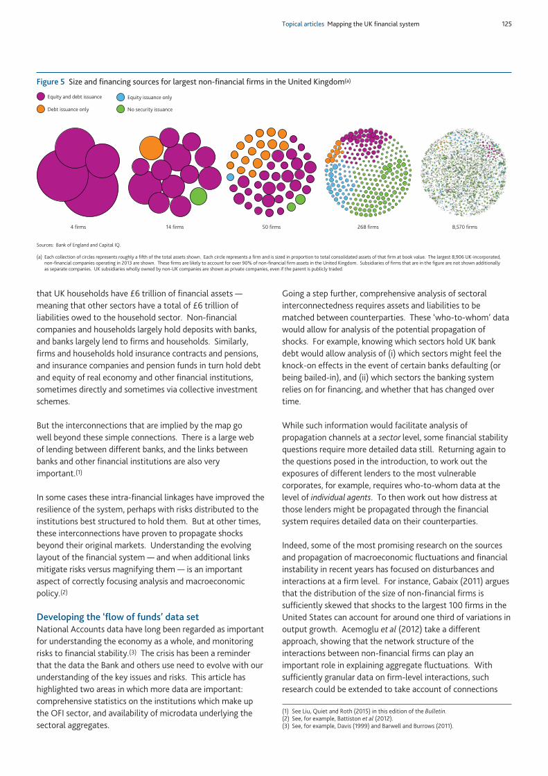
Figure 5 shows the largest non-financial firms in theUnited Kingdom. It shows less than 1% of companies (fewerthan 10,000 companies), but they likely account for over 90%of the total assets of all non-financial companies. Eachcollection of circles represents approximately one fifth of thetotal assets of the companies and each firm is represented bya circle sized proportionally to its assets. A small number ofvery large firms make up most of the aggregate balance sheetof the UK corporate sector. For example, the four largest firmshave total assets of roughly the same size as the nextfourteen.
Non-financial companies finance themselves in different ways:some (typically larger) firms have access to capital markets —they can issue debt (corporate bonds) or shares. Theremainder do not issue securities, so rely on other sourcessuch as retained earnings or bank loans for their financing. The
colour of the circles in Figure 5 corresponds to how the firmsfinance themselves. Only around 400 firms have bondsoutstanding and around 1,300 have publicly traded equity.
The prices of equities and bonds are watched carefully forinformation about the prospects of companies. But thisanalysis shows that this represents only a very small share ofUK companies by some measures, and it may not beappropriate to infer prospects for the whole corporate sectorfrom these markets. This might be important for the MPC’soutlook for growth and inflation in particular. For this reason,the Bank uses a variety of information sources to monitorfirms of different sizes, including microdata sources, surveyslike the Credit Conditions Survey and the Bank’s Agencynetwork.(1)
One of the questions posed in the introduction of this articleasked how vulnerable the most highly indebted corporates are.Data on individual firms can shed light on this. For instance,there may be significant numbers of firms in particularindustries that are vulnerable to shocks to income or interestrates. While it is possible to detect this with statisticalanalysis of the individual balance sheets, it may not be at allapparent from the aggregate balance sheet of thenon-financial company sector, as the high indebtedness ofsome areas of the corporate sector may be averaged out bylow indebtedness elsewhere.
To answer the final question posed in the introduction —who has lent to these vulnerable firms — requires furtherextensions of the currently available data. This is picked upin the next section.
Looking ahead: how can the data sets beimproved
Mapping out the links between the sectors: who isindebted to whom?As emphasised earlier in the article, financial assets andliabilities represent connections. But the data needed tocharacterise accurately these interconnections betweensectors are not always available. The map shows, for instance,
(1) Indeed, the Bank’s Credit Conditions Survey has persistently reported differentconditions for firms by size and highlighted different conditions for differentindustries. See England et al (2015) for more information on the work of theBank’s Agents.
Topical articles Mapping the UK financial system 125
that UK households have £6 trillion of financial assets —meaning that other sectors have a total of £6 trillion ofliabilities owed to the household sector. Non-financialcompanies and households largely hold deposits with banks,and banks largely lend to firms and households. Similarly,firms and households hold insurance contracts and pensions,and insurance companies and pension funds in turn hold debtand equity of real economy and other financial institutions,sometimes directly and sometimes via collective investmentschemes.
But the interconnections that are implied by the map gowell beyond these simple connections. There is a large webof lending between different banks, and the links betweenbanks and other financial institutions are also veryimportant.(1)
In some cases these intra-financial linkages have improved theresilience of the system, perhaps with risks distributed to theinstitutions best structured to hold them. But at other times,these interconnections have proven to propagate shocksbeyond their original markets. Understanding the evolvinglayout of the financial system — and when additional linksmitigate risks versus magnifying them — is an importantaspect of correctly focusing analysis and macroeconomicpolicy.(2)
Developing the ‘flow of funds’ data setNational Accounts data have long been regarded as importantfor understanding the economy as a whole, and monitoringrisks to financial stability.(3) The crisis has been a reminderthat the data the Bank and others use need to evolve with ourunderstanding of the key issues and risks. This article hashighlighted two areas in which more data are important:comprehensive statistics on the institutions which make upthe OFI sector, and availability of microdata underlying thesectoral aggregates.
Going a step further, comprehensive analysis of sectoralinterconnectedness requires assets and liabilities to bematched between counterparties. These ‘who-to-whom’ datawould allow for analysis of the potential propagation ofshocks. For example, knowing which sectors hold UK bankdebt would allow analysis of (i) which sectors might feel theknock-on effects in the event of certain banks defaulting (orbeing bailed-in), and (ii) which sectors the banking systemrelies on for financing, and whether that has changed overtime.
While such information would facilitate analysis ofpropagation channels at a sector level, some financial stabilityquestions require more detailed data still. Returning again tothe questions posed in the introduction, to work out theexposures of different lenders to the most vulnerablecorporates, for example, requires who-to-whom data at thelevel of individual agents. To then work out how distress atthose lenders might be propagated through the financialsystem requires detailed data on their counterparties.
Indeed, some of the most promising research on the sourcesand propagation of macroeconomic fluctuations and financialinstability in recent years has focused on disturbances andinteractions at a firm level. For instance, Gabaix (2011) arguesthat the distribution of the size of non-financial firms issufficiently skewed that shocks to the largest 100 firms in theUnited States can account for around one third of variations inoutput growth. Acemoglu et al (2012) take a differentapproach, showing that the network structure of theinteractions between non-financial firms can play animportant role in explaining aggregate fluctuations. Withsufficiently granular data on firm-level interactions, suchresearch could be extended to take account of connections
Equity and debt issuance
Debt issuance only
4 firms 14 firms 50 firms 268 firms 8,570 firms
Equity issuance only
No security issuance
Sources: Bank of England and Capital IQ.
(a) Each collection of circles represents roughly a fifth of the total assets shown. Each circle represents a firm and is sized in proportion to total consolidated assets of that firm at book value. The largest 8,906 UK-incorporated,non-financial companies operating in 2013 are shown. These firms are likely to account for over 90% of non-financial firm assets in the United Kingdom. Subsidiaries of firms that are in the figure are not shown additionallyas separate companies. UK subsidiaries wholly owned by non-UK companies are shown as private companies, even if the parent is publicly traded.
Figure 5 Size and financing sources for largest non-financial firms in the United Kingdom(a)
(1) See Liu, Quiet and Roth (2015) in this edition of the Bulletin.(2) See, for example, Battiston et al (2012).(3) See, for example, Davis (1999) and Barwell and Burrows (2011).
126 Quarterly Bulletin 2015 Q2
between the real economy and the financial system. AndDelli Gatti et al (2010) build a theoretical model in which acredit network exists both between firms and between firmsand banks, showing that the structure of this network ofinterconnections does indeed affect aggregate fluctuations.Further improvements in our understanding of financialinstability may require further improvements in our data.
This article has focused on the stock of financial assets andliabilities, but the same principles apply to flow data. Thecomplexity of the financial system could be better understoodwith collection of more detail on the OFI sector, availability ofmicrodata, and knowledge of who is transacting with whom.Sectoral Financial Accounts, covering both stocks and flows,compiled with counterparty information are often referred toas ‘Flow of Funds’ data.
The Bank of England and ONS are working together to makethe changes necessary to improve official Flow of Fundsdata.(1) For example, initiatives already under way include:undertaking an assessment of counterparty informationcurrently contained within the National Accounts; updatingthe surveys used to collect financial data so that estimation ofwho-to-whom relationships can be improved;(2) checking andimproving the classification of all financial firms surveyed; andenhancing the use of administrative and regulatory data toinform estimates.(3) At a minimum, this work is expected todeliver better interconnections data at a sectoral level andsome disaggregation of the OFI sector shown in Figure 2 intodifferent types of institutions. But it is possible that it will beable to go a lot further and use the underlying firm-level datato provide data sets for analysing risks within sectors, or eventhe interconnections between firms.
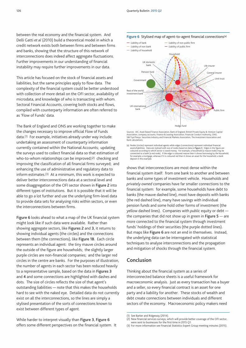
Figure 6 looks ahead to what a map of the UK financial systemmight look like if such data were available. Rather thanshowing aggregate sectors, like Figures 2 and 3, it returns toshowing individual agents (the circles) and the connectionsbetween them (the connections), like Figure 1B. Each circlerepresents an individual agent: the tiny mauve circles aroundthe outside of the figure are households; the slightly largerpurple circles are non-financial companies; and the larger redcircles in the centre are banks. For the purposes of illustration,the number of agents in each sector has been reduced heavilyto a representative sample, based on the data in Figures 3and 4 and some connections are highlighted with dashes anddots. The size of circles reflects the size of that agent’soutstanding liabilities — note that this makes the householdshard to see with the naked eye. Detailed data do not currentlyexist on all the interconnections, so the lines are simply astylised presentation of the sorts of connections known toexist between different types of agent.
While harder to interpret visually than Figure 3, Figure 6offers some different perspectives on the financial system. It
shows that interconnections are most dense within thefinancial system itself: from one bank to another and betweenbanks and some types of investment vehicle. Households andprivately owned companies have far smaller connections to thefinancial system: for example, some households have debt tobanks (the mauve dashed line), most have deposits with banks(the red dashed line), many have savings with individualpension funds and some hold other forms of investment (theyellow dashed lines). Companies with public equity or debt —the companies that did not show up in green in Figure 5— aremore connected to the financial system through investmentfunds’ holdings of their securities (the purple dotted lines).But maps like Figure 6 are not an end in themselves. Instead,the underlying data can be interrogated with statisticaltechniques to analyse interconnections and the propagationand mitigation of shocks through the financial system.
Conclusion
Thinking about the financial system as a series ofinterconnected balance sheets is a useful framework formacroeconomic analysis. Just as every transaction has a buyerand a seller, so every financial contract is an asset for oneparty and a liability for another. These stocks of wealth anddebt create connections between individuals and differentsectors of the economy. Macroeconomic policy makers need
Sources: AIC, Asset Based Finance Association, Bank of England, British Private Equity & Venture CapitalAssociation, company accounts, Finance & Leasing Association, Financial Conduct Authority, ONS,S&P SynThesys, Securities Industry and Financial Markets Association, The Investment Association andBank calculations.
(a) Nodes (circles) represent individual agents while edges (connections) represent individual financialassets/liabilities. Data are stylised with size of nodes based on data in Figure 3. Edges in the figure arecoloured according to which sector is owed money. For example, a household (a mauve node) may beconnected to a bank (a red node). If the edge is coloured mauve then it shows borrowing by the household,for example a mortgage, whereas if it is coloured red then it shows an asset for the household, a bankdeposit in this example.
(1) See Barker and Ridgeway (2014).(2) New financial services surveys, which will provide better coverage of the OFI sector,
were sent to businesses for the first time in 2015 Q1. (3) For more information see Financial Statistics Expert Group meeting minutes (2015).
Liability of bank
Liability of non-bank
Liability of household
Liability of non-public firm
Liability of public firm
Household
UK internationalbank
Rest of the worldinvestment bank
UK domesticbank
General insurer
Life insurer
Unit trust
Hedge fund
Public firm
Pension fund
Government
Figure 6 Stylised map of agent-to-agent financial connections(a)

Topical articles Mapping the UK financial system 127
to consider both sides of these connections. The various mapsexplored in this article use different sources of information topiece together the constituent sectors of the economy and area useful way of understanding how the financial system fitstogether.
It is important for the Bank of England to understand thisstock of financial wealth and debt, and the interconnections itrepresents. This work builds on the National Accounts of theUnited Kingdom and its focus reflects three areas in whichanalysis must push beyond traditional sources of data.
First, the financial system is not an amorphous whole and it isimportant to understand the different structures of non-bankfinancial companies. Sectoral balance sheets were introducedinto international standards for National Accounts in 1968.Financial systems have changed since then and, as a countrywith an important non-bank financial sector, it is natural thatthe United Kingdom should consider how that can best beencompassed into standard reporting.
Second, it is imperative to understand how these subsectorsof the financial system are connected to each other and toother parts of the economy. The maps are a way to ensurethat such analysis is not done for each type of institution inisolation, but rather considers how they fit into theUK economy.
Third, underlying differences can be as important assimilarities when analysing sectors. Some risks arise because awhole sector moves with the same trend — for example, thehigh levels of leverage that built up in banking systems acrossthe world prior to the global financial crisis. But others arisewhere aggregate data might not point to a risk — where asmall group of highly indebted borrowers or pockets ofvulnerable lenders arise, for example. Some risks will only beidentified by looking at high-level trends; while others will bemissed with such an approach requiring work with moredisaggregate data. Adjusting the map to the correct scale andfocus, and having the data to be able to do so as needed, areimportant elements of policy analysis.
128 Quarterly Bulletin 2015 Q2
References
Acemoglu, D, Carvalho, V, Ozdaglar, A and Tahbaz-Salehi, A (2012), ‘The network origins of aggregate fluctuations’, Econometrica, Vol. 80,No. 5, pages 1,977–2,016.
Balluck, K (2015), ‘Investment banking: linkages to the real economy and the financial system’, Bank of England Quarterly Bulletin, Vol. 55,No. 1, pages 4–22, available at www.bankofengland.co.uk/publications/Documents/quarterlybulletin/2015/q101.pdf.
Barker, K and Ridgeway, A (2014), ‘National Accounts and balance of payments’, National Statistics Quality Review, Series 2, Report 2.
Barwell, R and Burrows, O (2011), ‘Growing fragilities? Balance sheets in The Great Moderation’, Bank of England Financial Stability PaperNo. 10, available at www.bankofengland.co.uk/research/Documents/fspapers/fs_paper10.pdf.
Battiston, S, Delli Gatti, D, Gallegati, M, Greenwald, B and Stiglitz, J E (2012), ‘Liaisons dangereuses: increasing connectivity, risk sharing, andsystemic risk’, Journal of Economic Dynamics and Control, Vol. 36, pages 1,121–41.
Breckenridge, J, Farquharson, J and Hendon, R (2014), ‘The role of business model analysis in the supervision of insurers’, Bank of EnglandQuarterly Bulletin, Vol. 54, No. 1, pages 49–57, available at www.bankofengland.co.uk/publications/Documents/quarterlybulletin/2014/qb14q105.pdf.
Bush, O, Knott, S and Peacock, C (2014), ‘Why is the UK banking system so big and is that a problem?’, Bank of England Quarterly Bulletin,Vol. 54, No. 4, pages 385–95, available at www.bankofengland.co.uk/publications/Documents/quarterlybulletin/2014/qb14q402.pdf.
Cumming, F and Noss, J (2013), ‘Assessing the adequacy of CCPs’ default resources’, Bank of England Financial Stability Paper No. 26, available at www.bankofengland.co.uk/research/Documents/fspapers/fs_paper26.pdf.
Davies, R, Katinaite, V, Manning, M and Richardson, P (2010), ‘Evolution of the UK banking system’, Bank of England Quarterly Bulletin,Vol. 50, No. 4, pages 321–32, available at www.bankofengland.co.uk/publications/Documents/quarterlybulletin/qb100407.pdf.
Davis, E P (1999), ‘Financial data needs for macroprudential surveillance — what are the key indicators of risks to domestic financial stability?’,Handbooks in Central Banking, Centre for Central Banking Studies, Bank of England, available atwww.bankofengland.co.uk/education/Documents/ccbs/ls/pdf/lshb02.pdf.
Delli Gatti, D, Gallegati, M, Greenwald, B, Russo, A and Stiglitz, J (2010), ‘The financial accelerator in an evolving credit network’, Journal of Economic Dynamics and Control, Vol. 34, Issue 9, pages 1,627–50.
England, D, Hebden, A, Henderson, T and Pattie, T (2015), ‘The Agencies and ‘One Bank’’, Bank of England Quarterly Bulletin, Vol. 55, No. 1,pages 47–55, available at www.bankofengland.co.uk/publications/Documents/quarterlybulletin/2015/q104.pdf.
Farag, M, Harland, D and Nixon, D (2013), ‘Bank capital and liquidity’, Bank of England Quarterly Bulletin, Vol. 53, No. 3, pages 201–15,available at www.bankofengland.co.uk/publications/Documents/quarterlybulletin/2013/qb130302.pdf.
Financial Statistics Expert Group (2015), January 22nd meeting minutes, available at www.ons.gov.uk/ons/guide-method/method-quality/specific/economy/national-accounts/changes-to-national-accounts/flow-of-funds--fof-/fseg-minutes-22-january-2015.doc.
Gabaix, X (2011), ‘The granular origins of aggregate fluctuations’, Econometrica, Vol. 79, No. 3, pages 733–72.
Gregory, D (2013), ‘Private equity and financial stability’, Bank of England Quarterly Bulletin, Vol. 53, No. 1, pages 38–47, available atwww.bankofengland.co.uk/publications/Documents/quarterlybulletin/2013/qb130104.pdf.
Liu, Z, Quiet, S and Roth, B (2015), ‘Banking sector interconnectedness: what is it, how can we measure it and why does it matter?’,Bank of England Quarterly Bulletin, Vol. 55, No. 2, pages 130–38, available atwww.bankofengland.co.uk/publications/Documents/quarterlybulletin/2015/q202.pdf.
McLeay, M, Radia, A and Thomas, R (2014), ‘Money creation in the modern economy’, Bank of England Quarterly Bulletin, Vol. 54, No. 1,pages 14–27, available at www.bankofengland.co.uk/publications/Documents/quarterlybulletin/2014/qb14q102.pdf.
Piketty, T, translated by Goldhammer, A (2014), Capital in the twenty-first century, The Belknap Press of Harvard University Press.

Topical articles Mapping the UK financial system 129
Pozsar, Z, Adrian, T, Ashcroft, A and Boesky, H (2010), ‘Shadow banking’, Federal Reserve Bank of New York Staff Report, No. 458.
Radcliffe Report (1959), ‘Committee on the working of the monetary system’, Cmnd 827, HMSO, London.
Rehlon, A and Nixon, D (2013), ‘Central counterparties: what are they, why do they matter and how does the Bank supervise them?’, Bank of England Quarterly Bulletin, Vol. 53, No. 2, pages 147–56,available at www.bankofengland.co.uk/publications/Documents/quarterlybulletin/2013/qb130206.pdf.
Williams, A and Martin, G (eds) (2002), Domesday Book: a complete translation, London.
Wilson Report (1980), ‘Committee to review the functioning of financial institutions’, Cmnd 7937, HMSO, London.
130 Quarterly Bulletin 2015 Q2
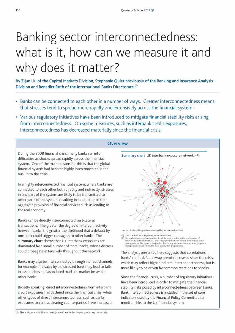
• Banks can be connected to each other in a number of ways. Greater interconnectedness meansthat stresses tend to spread more rapidly and extensively across the financial system.
• Various regulatory initiatives have been introduced to mitigate financial stability risks arisingfrom interconnectedness. On some measures, such as interbank credit exposures,interconnectedness has decreased materially since the financial crisis.
Banking sector interconnectedness:what is it, how can we measure it andwhy does it matter?By Zijun Liu of the Capital Markets Division, Stephanie Quiet previously of the Banking and Insurance AnalysisDivision and Benedict Roth of the International Banks Directorate.(1)
Overview
During the 2008 financial crisis, many banks ran intodifficulties as shocks spread rapidly across the financialsystem. One of the main reasons for this is that the globalfinancial system had become highly interconnected in therun-up to the crisis.
In a highly interconnected financial system, where banks areconnected to each other both directly and indirectly, stressesin one part of the system are likely to be transmitted toother parts of the system, resulting in a reduction in theaggregate provision of financial services such as lending tothe real economy.
Banks can be directly interconnected via bilateraltransactions. The greater the degree of interconnectivitybetween banks, the greater the likelihood that a default byone bank could trigger contagion to other banks. Thesummary chart shows that UK interbank exposures aredominated by a small number of ‘core’ banks, whose distresscould propagate extensively throughout the network.
Banks may also be interconnected through indirect channels:for example, fire sales by a distressed bank may lead to fallsin asset prices and associated mark-to-market losses forother banks.
Broadly speaking, direct interconnectedness from interbankcredit exposures has declined since the financial crisis, whileother types of direct interconnectedness, such as banks’exposures to central clearing counterparties, have increased.
The analysis presented here suggests that correlations inbanks’ credit default swap premia increased since the crisis,which may reflect higher indirect interconnectedness, but ismore likely to be driven by common reactions to shocks.
Since the financial crisis, a number of regulatory initiativeshave been introduced in order to mitigate the financialstability risks posed by interconnectedness between banks.Bank interconnectedness is included in the set of coreindicators used by the Financial Policy Committee tomonitor risks to the UK financial system.
Summary chart UK interbank exposure network(a)(b)
Sources: Prudential Regulation Authority (PRA) and Bank calculations.
(a) Data as at end-2013. Exposures are net of collateral.(b) Each node represents a bank and the size of the node is scaled by the total amount of
exposures to and from that bank. Each arrow points from one bank to another bank that ithas exposure to. The layout is designed so that for any two banks in the network, the greaterthe exposures between them, the more closely they are positioned.
(1) The authors would like to thank Jamie Coen for his help in producing this article.
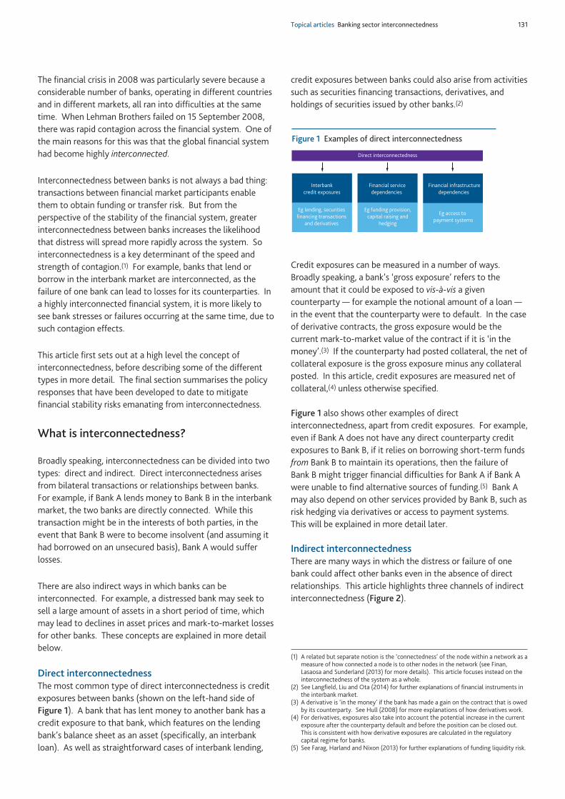
Topical articles Banking sector interconnectedness 131
The financial crisis in 2008 was particularly severe because aconsiderable number of banks, operating in different countriesand in different markets, all ran into difficulties at the sametime. When Lehman Brothers failed on 15 September 2008,there was rapid contagion across the financial system. One ofthe main reasons for this was that the global financial systemhad become highly interconnected.
Interconnectedness between banks is not always a bad thing:transactions between financial market participants enablethem to obtain funding or transfer risk. But from theperspective of the stability of the financial system, greaterinterconnectedness between banks increases the likelihoodthat distress will spread more rapidly across the system. Sointerconnectedness is a key determinant of the speed andstrength of contagion.(1) For example, banks that lend orborrow in the interbank market are interconnected, as thefailure of one bank can lead to losses for its counterparties. Ina highly interconnected financial system, it is more likely tosee bank stresses or failures occurring at the same time, due tosuch contagion effects.
This article first sets out at a high level the concept ofinterconnectedness, before describing some of the differenttypes in more detail. The final section summarises the policyresponses that have been developed to date to mitigatefinancial stability risks emanating from interconnectedness.
What is interconnectedness?
Broadly speaking, interconnectedness can be divided into twotypes: direct and indirect. Direct interconnectedness arisesfrom bilateral transactions or relationships between banks.For example, if Bank A lends money to Bank B in the interbankmarket, the two banks are directly connected. While thistransaction might be in the interests of both parties, in theevent that Bank B were to become insolvent (and assuming ithad borrowed on an unsecured basis), Bank A would sufferlosses.
There are also indirect ways in which banks can beinterconnected. For example, a distressed bank may seek tosell a large amount of assets in a short period of time, whichmay lead to declines in asset prices and mark-to-market lossesfor other banks. These concepts are explained in more detailbelow.
Direct interconnectednessThe most common type of direct interconnectedness is creditexposures between banks (shown on the left-hand side ofFigure 1). A bank that has lent money to another bank has acredit exposure to that bank, which features on the lendingbank’s balance sheet as an asset (specifically, an interbankloan). As well as straightforward cases of interbank lending,
credit exposures between banks could also arise from activitiessuch as securities financing transactions, derivatives, andholdings of securities issued by other banks.(2)
Credit exposures can be measured in a number of ways.Broadly speaking, a bank’s ‘gross exposure’ refers to theamount that it could be exposed to vis-à-vis a givencounterparty — for example the notional amount of a loan —in the event that the counterparty were to default. In the caseof derivative contracts, the gross exposure would be thecurrent mark-to-market value of the contract if it is ‘in themoney’.(3) If the counterparty had posted collateral, the net ofcollateral exposure is the gross exposure minus any collateralposted. In this article, credit exposures are measured net ofcollateral,(4) unless otherwise specified.
Figure 1 also shows other examples of directinterconnectedness, apart from credit exposures. For example,even if Bank A does not have any direct counterparty creditexposures to Bank B, if it relies on borrowing short-term fundsfrom Bank B to maintain its operations, then the failure ofBank B might trigger financial difficulties for Bank A if Bank Awere unable to find alternative sources of funding.(5) Bank Amay also depend on other services provided by Bank B, such asrisk hedging via derivatives or access to payment systems.This will be explained in more detail later.
Indirect interconnectednessThere are many ways in which the distress or failure of onebank could affect other banks even in the absence of directrelationships. This article highlights three channels of indirectinterconnectedness (Figure 2).
(1) A related but separate notion is the ‘connectedness’ of the node within a network as ameasure of how connected a node is to other nodes in the network (see Finan,Lasaosa and Sunderland (2013) for more details). This article focuses instead on theinterconnectedness of the system as a whole.
(2) See Langfield, Liu and Ota (2014) for further explanations of financial instruments inthe interbank market.
(3) A derivative is ‘in the money’ if the bank has made a gain on the contract that is owedby its counterparty. See Hull (2008) for more explanations of how derivatives work.
(4) For derivatives, exposures also take into account the potential increase in the currentexposure after the counterparty default and before the position can be closed out.This is consistent with how derivative exposures are calculated in the regulatorycapital regime for banks.
(5) See Farag, Harland and Nixon (2013) for further explanations of funding liquidity risk.
Assets
Direct interconnectedness
Interbankcredit exposures
Financial servicedependencies
Eg funding provision,capital raising and
hedging
Eg access to payment systems
Eg lending, securitiesfinancing transactions
and derivatives
Financial infrastructuredependencies
Figure 1 Examples of direct interconnectedness
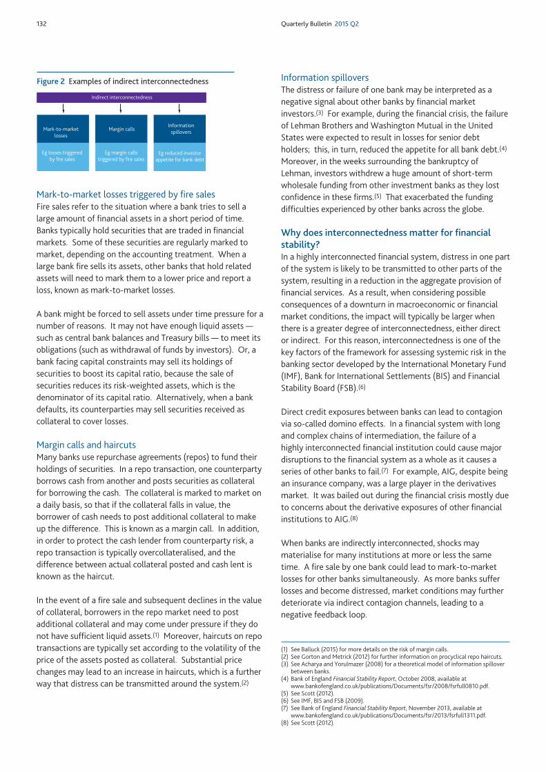
132 Quarterly Bulletin 2015 Q2
Mark-to-market losses triggered by fire salesFire sales refer to the situation where a bank tries to sell alarge amount of financial assets in a short period of time.Banks typically hold securities that are traded in financialmarkets. Some of these securities are regularly marked tomarket, depending on the accounting treatment. When alarge bank fire sells its assets, other banks that hold relatedassets will need to mark them to a lower price and report aloss, known as mark-to-market losses.
A bank might be forced to sell assets under time pressure for anumber of reasons. It may not have enough liquid assets —such as central bank balances and Treasury bills — to meet itsobligations (such as withdrawal of funds by investors). Or, abank facing capital constraints may sell its holdings ofsecurities to boost its capital ratio, because the sale ofsecurities reduces its risk-weighted assets, which is thedenominator of its capital ratio. Alternatively, when a bankdefaults, its counterparties may sell securities received ascollateral to cover losses.
Margin calls and haircuts Many banks use repurchase agreements (repos) to fund theirholdings of securities. In a repo transaction, one counterpartyborrows cash from another and posts securities as collateralfor borrowing the cash. The collateral is marked to market ona daily basis, so that if the collateral falls in value, theborrower of cash needs to post additional collateral to makeup the difference. This is known as a margin call. In addition,in order to protect the cash lender from counterparty risk, arepo transaction is typically overcollateralised, and thedifference between actual collateral posted and cash lent isknown as the haircut.
In the event of a fire sale and subsequent declines in the valueof collateral, borrowers in the repo market need to postadditional collateral and may come under pressure if they donot have sufficient liquid assets.(1) Moreover, haircuts on repotransactions are typically set according to the volatility of theprice of the assets posted as collateral. Substantial pricechanges may lead to an increase in haircuts, which is a furtherway that distress can be transmitted around the system.(2)
Information spillovers The distress or failure of one bank may be interpreted as anegative signal about other banks by financial marketinvestors.(3) For example, during the financial crisis, the failureof Lehman Brothers and Washington Mutual in the UnitedStates were expected to result in losses for senior debtholders; this, in turn, reduced the appetite for all bank debt.(4)
Moreover, in the weeks surrounding the bankruptcy ofLehman, investors withdrew a huge amount of short-termwholesale funding from other investment banks as they lostconfidence in these firms.(5) That exacerbated the fundingdifficulties experienced by other banks across the globe.
Why does interconnectedness matter for financialstability?In a highly interconnected financial system, distress in one partof the system is likely to be transmitted to other parts of thesystem, resulting in a reduction in the aggregate provision offinancial services. As a result, when considering possibleconsequences of a downturn in macroeconomic or financialmarket conditions, the impact will typically be larger whenthere is a greater degree of interconnectedness, either director indirect. For this reason, interconnectedness is one of thekey factors of the framework for assessing systemic risk in thebanking sector developed by the International Monetary Fund(IMF), Bank for International Settlements (BIS) and FinancialStability Board (FSB).(6)
Direct credit exposures between banks can lead to contagionvia so-called domino effects. In a financial system with longand complex chains of intermediation, the failure of ahighly interconnected financial institution could cause majordisruptions to the financial system as a whole as it causes aseries of other banks to fail.(7) For example, AIG, despite beingan insurance company, was a large player in the derivativesmarket. It was bailed out during the financial crisis mostly dueto concerns about the derivative exposures of other financialinstitutions to AIG.(8)
When banks are indirectly interconnected, shocks maymaterialise for many institutions at more or less the sametime. A fire sale by one bank could lead to mark-to-marketlosses for other banks simultaneously. As more banks sufferlosses and become distressed, market conditions may furtherdeteriorate via indirect contagion channels, leading to anegative feedback loop.
Assets
Indirect interconnectedness
Mark-to-marketlosses
Financial service and infrastructuredependencies
Margin callsInformation
spillovers
Eg losses triggeredby fire sales
Eg reduced investorappetite for bank debt
Eg margin callstriggered by fire sales
Figure 2 Examples of indirect interconnectedness
(1) See Balluck (2015) for more details on the risk of margin calls.(2) See Gorton and Metrick (2012) for further information on procyclical repo haircuts.(3) See Acharya and Yorulmazer (2008) for a theoretical model of information spillover
between banks.(4) Bank of England Financial Stability Report, October 2008, available at
www.bankofengland.co.uk/publications/Documents/fsr/2008/fsrfull0810.pdf.(5) See Scott (2012).(6) See IMF, BIS and FSB (2009).(7) See Bank of England Financial Stability Report, November 2013, available at
www.bankofengland.co.uk/publications/Documents/fsr/2013/fsrfull1311.pdf.(8) See Scott (2012).
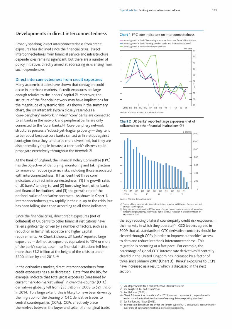
Topical articles Banking sector interconnectedness 133
Developments in direct interconnectedness
Broadly speaking, direct interconnectedness from creditexposures has declined since the financial crisis. Directinterconnectedness from financial service and infrastructuredependencies remains significant, but there are a number ofpolicy initiatives directly aimed at addressing risks arising fromsuch dependencies.
Direct interconnectedness from credit exposuresMany academic studies have shown that contagion couldoccur in interbank markets, if credit exposures are largeenough relative to the lenders’ capital.(1) Moreover, thestructure of the financial network may have implications forthe magnitude of systemic risks. As shown in the summarychart, the UK interbank system closely resembles a‘core-periphery’ network, in which ‘core’ banks are connectedto all banks in the network and peripheral banks are onlyconnected to the ‘core’ banks.(2) Core-periphery networkstructures possess a ‘robust-yet-fragile’ property — they tendto be robust because core banks can act as fire-stops againstcontagion since they tend to be more diversified, but they arealso potentially fragile because a core bank’s distress couldpropagate extensively throughout the network.(3)
At the Bank of England, the Financial Policy Committee (FPC)has the objective of identifying, monitoring and taking actionto remove or reduce systemic risks, including those associatedwith interconnectedness. It has identified three coreindicators on direct interconnectedness: (1) the growth ratesof UK banks’ lending to, and (2) borrowing from, other banksand financial institutions; and (3) the growth rate of thenotional value of derivative contracts. As shown in Chart 1,interconnectedness grew rapidly in the run-up to the crisis, buthas been falling since then according to all three indicators.
Since the financial crisis, direct credit exposures (net ofcollateral) of UK banks to other financial institutions havefallen significantly, driven by a number of factors, such as areduction in firms’ risk appetite and higher capitalrequirements. As Chart 2 shows, UK banks’ reported largeexposures — defined as exposures equivalent to 10% or moreof the bank’s capital base — to financial institutions fell frommore than £1.2 trillion at the height of the crisis to under£200 billion by end-2013.(4)
In the derivatives market, direct interconnectedness fromcredit exposures has also decreased. Data from the BIS, forexample, indicate that total gross exposures (measured bycurrent mark-to-market values) in over-the-counter (OTC)derivatives globally fell from $35 trillion in 2008 to $21 trillionin 2014. To a large extent, this is likely to have been driven bythe migration of the clearing of OTC derivative trades tocentral counterparties (CCPs). CCPs effectively placethemselves between the buyer and seller of an original trade,
thereby reducing bilateral counterparty credit risk exposures inthe markets in which they operate.(5) G20 leaders agreed in2009 that all standardised OTC derivative contracts should becleared through CCPs in order to improve authorities’ accessto data and reduce interbank interconnectedness. Thismigration is occurring at a fast pace. For example, thepercentage of global OTC interest rate derivatives(6) centrallycleared in the United Kingdom has increased by a factor ofthree since January 2007 (Chart 3). Banks’ exposures to CCPshave increased as a result, which is discussed in the nextsection.
30
20
10
0
10
20
30
40
50
60
2002 03 04 05 06 07 08 09 10 11 12 13 14
Annual growth in banks’ lending to other banks and financial institutionsAnnual growth in banks’ borrowing from other banks and financial institutions
Annual growth in notional derivative positions Per cent
+
–
Sources: Published accounts and Bank calculations.
Chart 1 FPC core indicators on interconnectedness
(1) See Upper (2010) for a comprehensive literature review.(2) See Langfield, Liu and Ota (2014).(3) See Haldane (2009).(4) Chart 2 does not include data after 2013 because they are not comparable with
earlier data due to the introduction of new regulatory reporting standards.(5) See Rehlon and Nixon (2013).(6) Interest rate derivatives are by far the largest type of OTC derivatives, accounting for
over 80% of outstanding notional derivatives positions.
0
200
400
600
800
1,000
1,200
1,400 £ billions
Q3 Q1 Q3 Q1 Q3 Q1 Q3 Q1 Q3 Q1Q3 Q1 Q32008 09 10 11 12 13
Sources: PRA and Bank calculations.
(a) Sum of all large exposures to financial institutions reported by UK banks. Exposures are netof credit risk mitigation.
(b) Only exposures equivalent to 10% or more of a given bank’s capital are reported, so declinesin reported exposures may be driven by higher capital, a reduction in the concentration ofexposures, or both.
Chart 2 UK banks’ reported large exposures (net ofcollateral) to other financial institutions(a)(b)
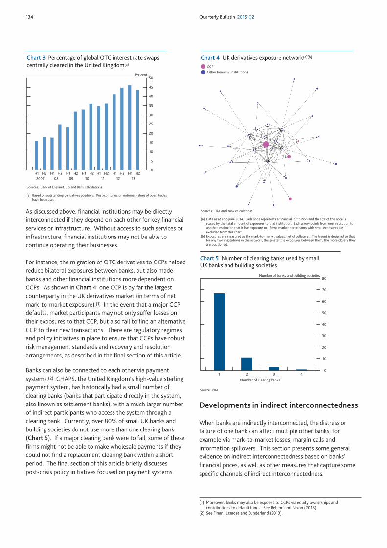
134 Quarterly Bulletin 2015 Q2
As discussed above, financial institutions may be directlyinterconnected if they depend on each other for key financialservices or infrastructure. Without access to such services orinfrastructure, financial institutions may not be able tocontinue operating their businesses.
For instance, the migration of OTC derivatives to CCPs helpedreduce bilateral exposures between banks, but also madebanks and other financial institutions more dependent onCCPs. As shown in Chart 4, one CCP is by far the largestcounterparty in the UK derivatives market (in terms of netmark-to-market exposure).(1) In the event that a major CCPdefaults, market participants may not only suffer losses ontheir exposures to that CCP, but also fail to find an alternativeCCP to clear new transactions. There are regulatory regimesand policy initiatives in place to ensure that CCPs have robustrisk management standards and recovery and resolutionarrangements, as described in the final section of this article.
Banks can also be connected to each other via paymentsystems.(2) CHAPS, the United Kingdom’s high-value sterlingpayment system, has historically had a small number ofclearing banks (banks that participate directly in the system,also known as settlement banks), with a much larger numberof indirect participants who access the system through aclearing bank. Currently, over 80% of small UK banks andbuilding societies do not use more than one clearing bank(Chart 5). If a major clearing bank were to fail, some of thesefirms might not be able to make wholesale payments if theycould not find a replacement clearing bank within a shortperiod. The final section of this article briefly discussespost-crisis policy initiatives focused on payment systems.
Developments in indirect interconnectedness
When banks are indirectly interconnected, the distress orfailure of one bank can affect multiple other banks, forexample via mark-to-market losses, margin calls andinformation spillovers. This section presents some generalevidence on indirect interconnectedness based on banks’financial prices, as well as other measures that capture somespecific channels of indirect interconnectedness.
0
5
10
15
20
25
30
35
40
45
50Per cent
H1 H2 H1 H2 H1 H2 H1 H2 H1 H2 H1 H2 H1 H22007 08 09 10 11 12 13
Sources: Bank of England, BIS and Bank calculations.
(a) Based on outstanding derivatives positions. Post-compression notional values of open tradeshave been used.
Chart 3 Percentage of global OTC interest rate swapscentrally cleared in the United Kingdom(a) CCP
Other financial institutions
Sources: PRA and Bank calculations.
(a) Data as at end-June 2014. Each node represents a financial institution and the size of the node isscaled by the total amount of exposures to that institution. Each arrow points from one institution toanother institution that it has exposure to. Some market participants with small exposures areexcluded from this chart.
(b) Exposures are measured as the mark-to-market values, net of collateral. The layout is designed so thatfor any two institutions in the network, the greater the exposures between them, the more closely theyare positioned.
Chart 4 UK derivatives exposure network(a)(b)
(1) Moreover, banks may also be exposed to CCPs via equity ownerships andcontributions to default funds. See Rehlon and Nixon (2013).
(2) See Finan, Lasaosa and Sunderland (2013).
0
10
20
30
40
50
60
70
80
1 2 3 4Number of clearing banks
Number of banks and building societies
Source: PRA.
Chart 5 Number of clearing banks used by smallUK banks and building societies
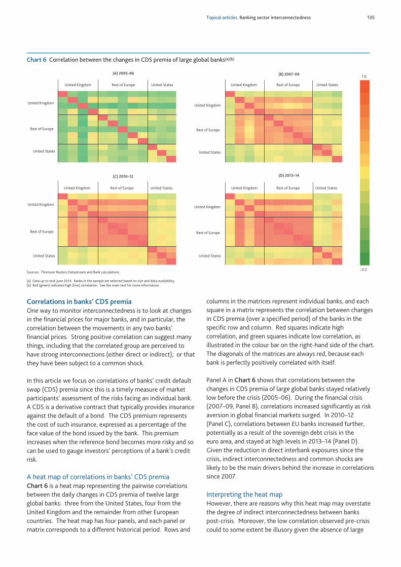
Topical articles Banking sector interconnectedness 135
Correlations in banks’ CDS premiaOne way to monitor interconnectedness is to look at changesin the financial prices for major banks, and in particular, thecorrelation between the movements in any two banks’financial prices. Strong positive correlation can suggest manythings, including that the correlated group are perceived tohave strong interconnections (either direct or indirect); or thatthey have been subject to a common shock.
In this article we focus on correlations of banks’ credit defaultswap (CDS) premia since this is a timely measure of marketparticipants’ assessment of the risks facing an individual bank.A CDS is a derivative contract that typically provides insuranceagainst the default of a bond. The CDS premium representsthe cost of such insurance, expressed as a percentage of theface value of the bond issued by the bank. This premiumincreases when the reference bond becomes more risky and socan be used to gauge investors’ perceptions of a bank’s creditrisk.
A heat map of correlations in banks’ CDS premiaChart 6 is a heat map representing the pairwise correlationsbetween the daily changes in CDS premia of twelve largeglobal banks: three from the United States, four from theUnited Kingdom and the remainder from other Europeancountries. The heat map has four panels, and each panel ormatrix corresponds to a different historical period. Rows and
columns in the matrices represent individual banks, and eachsquare in a matrix represents the correlation between changesin CDS premia (over a specified period) of the banks in thespecific row and column. Red squares indicate highcorrelation, and green squares indicate low correlation, asillustrated in the colour bar on the right-hand side of the chart.The diagonals of the matrices are always red, because eachbank is perfectly positively correlated with itself.
Panel A in Chart 6 shows that correlations between thechanges in CDS premia of large global banks stayed relativelylow before the crisis (2005–06). During the financial crisis(2007–09, Panel B), correlations increased significantly as riskaversion in global financial markets surged. In 2010–12(Panel C), correlations between EU banks increased further,potentially as a result of the sovereign debt crisis in theeuro area, and stayed at high levels in 2013–14 (Panel D).Given the reduction in direct interbank exposures since thecrisis, indirect interconnectedness and common shocks arelikely to be the main drivers behind the increase in correlationssince 2007.
Interpreting the heat mapHowever, there are reasons why this heat map may overstatethe degree of indirect interconnectedness between bankspost-crisis. Moreover, the low correlation observed pre-crisiscould to some extent be illusory given the absence of large
United States
Rest of Europe
United Kingdom
(B) 2007–09
(C) 2010–12 (D) 2013–14
United Kingdom Rest of Europe United States
(A) 2005–06
United States
Rest of Europe
United Kingdom
United Kingdom Rest of Europe United States
United States
Rest of Europe
United Kingdom
United Kingdom Rest of Europe United States
United States
Rest of Europe
United Kingdom
United Kingdom Rest of Europe United States
1.0
-0.2Sources: Thomson Reuters Datastream and Bank calculations.
(a) Data up to end-June 2014. Banks in the sample are selected based on size and data availability.(b) Red (green) indicates high (low) correlation. See the main text for more information.
Chart 6 Correlation between the changes in CDS premia of large global banks(a)(b)
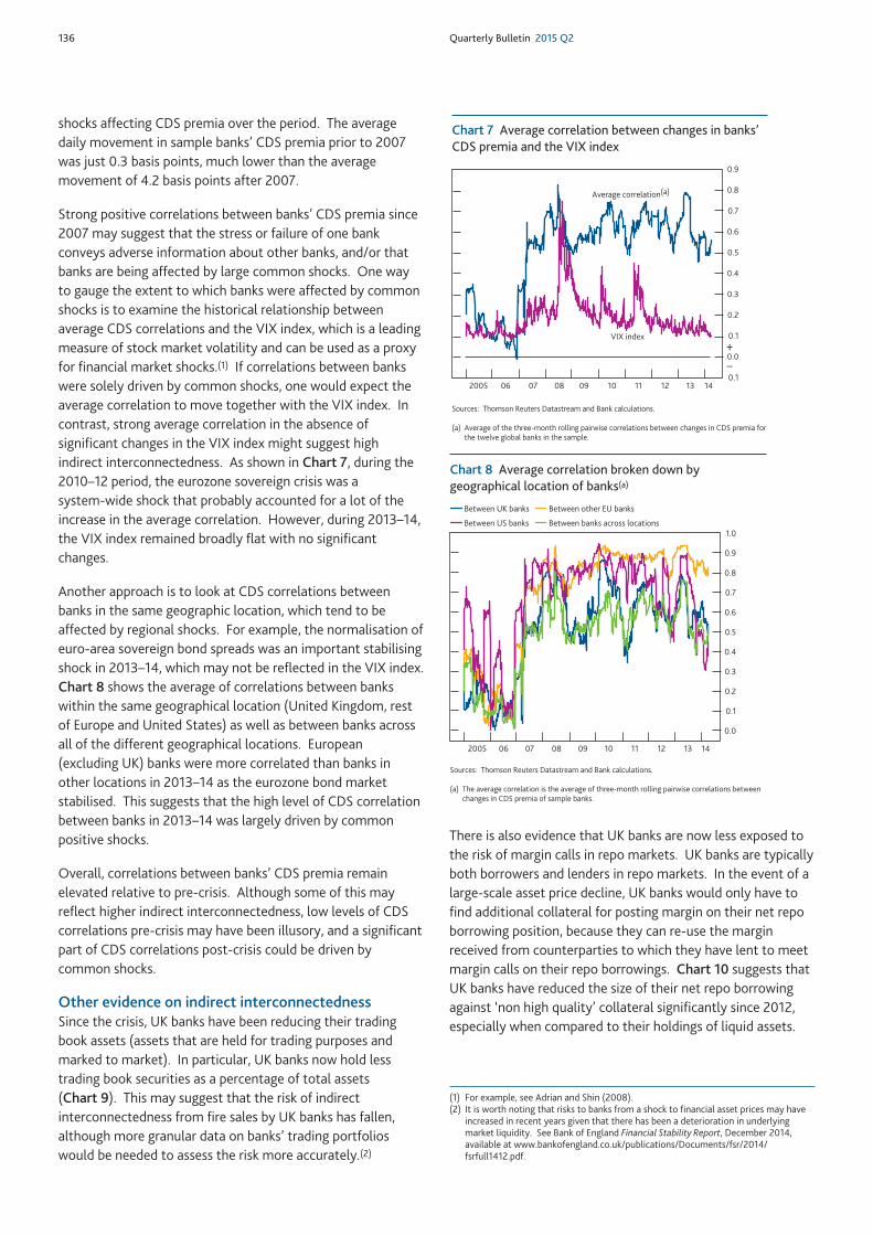
136 Quarterly Bulletin 2015 Q2
shocks affecting CDS premia over the period. The averagedaily movement in sample banks’ CDS premia prior to 2007was just 0.3 basis points, much lower than the averagemovement of 4.2 basis points after 2007.
Strong positive correlations between banks’ CDS premia since2007 may suggest that the stress or failure of one bankconveys adverse information about other banks, and/or thatbanks are being affected by large common shocks. One wayto gauge the extent to which banks were affected by commonshocks is to examine the historical relationship betweenaverage CDS correlations and the VIX index, which is a leadingmeasure of stock market volatility and can be used as a proxyfor financial market shocks.(1) If correlations between bankswere solely driven by common shocks, one would expect theaverage correlation to move together with the VIX index. Incontrast, strong average correlation in the absence ofsignificant changes in the VIX index might suggest highindirect interconnectedness. As shown in Chart 7, during the2010–12 period, the eurozone sovereign crisis was asystem-wide shock that probably accounted for a lot of theincrease in the average correlation. However, during 2013–14,the VIX index remained broadly flat with no significantchanges.
Another approach is to look at CDS correlations betweenbanks in the same geographic location, which tend to beaffected by regional shocks. For example, the normalisation ofeuro-area sovereign bond spreads was an important stabilisingshock in 2013–14, which may not be reflected in the VIX index.Chart 8 shows the average of correlations between bankswithin the same geographical location (United Kingdom, restof Europe and United States) as well as between banks acrossall of the different geographical locations. European(excluding UK) banks were more correlated than banks inother locations in 2013–14 as the eurozone bond marketstabilised. This suggests that the high level of CDS correlationbetween banks in 2013–14 was largely driven by commonpositive shocks.
Overall, correlations between banks’ CDS premia remainelevated relative to pre-crisis. Although some of this mayreflect higher indirect interconnectedness, low levels of CDScorrelations pre-crisis may have been illusory, and a significantpart of CDS correlations post-crisis could be driven bycommon shocks.
Other evidence on indirect interconnectednessSince the crisis, UK banks have been reducing their tradingbook assets (assets that are held for trading purposes andmarked to market). In particular, UK banks now hold lesstrading book securities as a percentage of total assets(Chart 9). This may suggest that the risk of indirectinterconnectedness from fire sales by UK banks has fallen,although more granular data on banks’ trading portfolioswould be needed to assess the risk more accurately.(2)
There is also evidence that UK banks are now less exposed tothe risk of margin calls in repo markets. UK banks are typicallyboth borrowers and lenders in repo markets. In the event of alarge-scale asset price decline, UK banks would only have tofind additional collateral for posting margin on their net repoborrowing position, because they can re-use the marginreceived from counterparties to which they have lent to meetmargin calls on their repo borrowings. Chart 10 suggests thatUK banks have reduced the size of their net repo borrowingagainst ‘non high quality’ collateral significantly since 2012,especially when compared to their holdings of liquid assets.
0.1
0.0
0.1
0.2
0.3
0.4
0.5
0.6
0.7
0.8
0.9
2005 06 07 08 09 10 11 12 13 14
Average correlation(a)
VIX index +
–
Sources: Thomson Reuters Datastream and Bank calculations.
(a) Average of the three-month rolling pairwise correlations between changes in CDS premia forthe twelve global banks in the sample.
Chart 7 Average correlation between changes in banks’CDS premia and the VIX index
(1) For example, see Adrian and Shin (2008).(2) It is worth noting that risks to banks from a shock to financial asset prices may have
increased in recent years given that there has been a deterioration in underlyingmarket liquidity. See Bank of England Financial Stability Report, December 2014,available at www.bankofengland.co.uk/publications/Documents/fsr/2014/fsrfull1412.pdf.
0.0
0.1
0.2
0.3
0.4
0.5
0.6
0.7
0.8
0.9
1.0
2005 06 07 08 09 10 11 12 13 14
Between UK banks Between other EU banks
Between US banks Between banks across locations
Sources: Thomson Reuters Datastream and Bank calculations.
(a) The average correlation is the average of three-month rolling pairwise correlations betweenchanges in CDS premia of sample banks.
Chart 8 Average correlation broken down bygeographical location of banks(a)
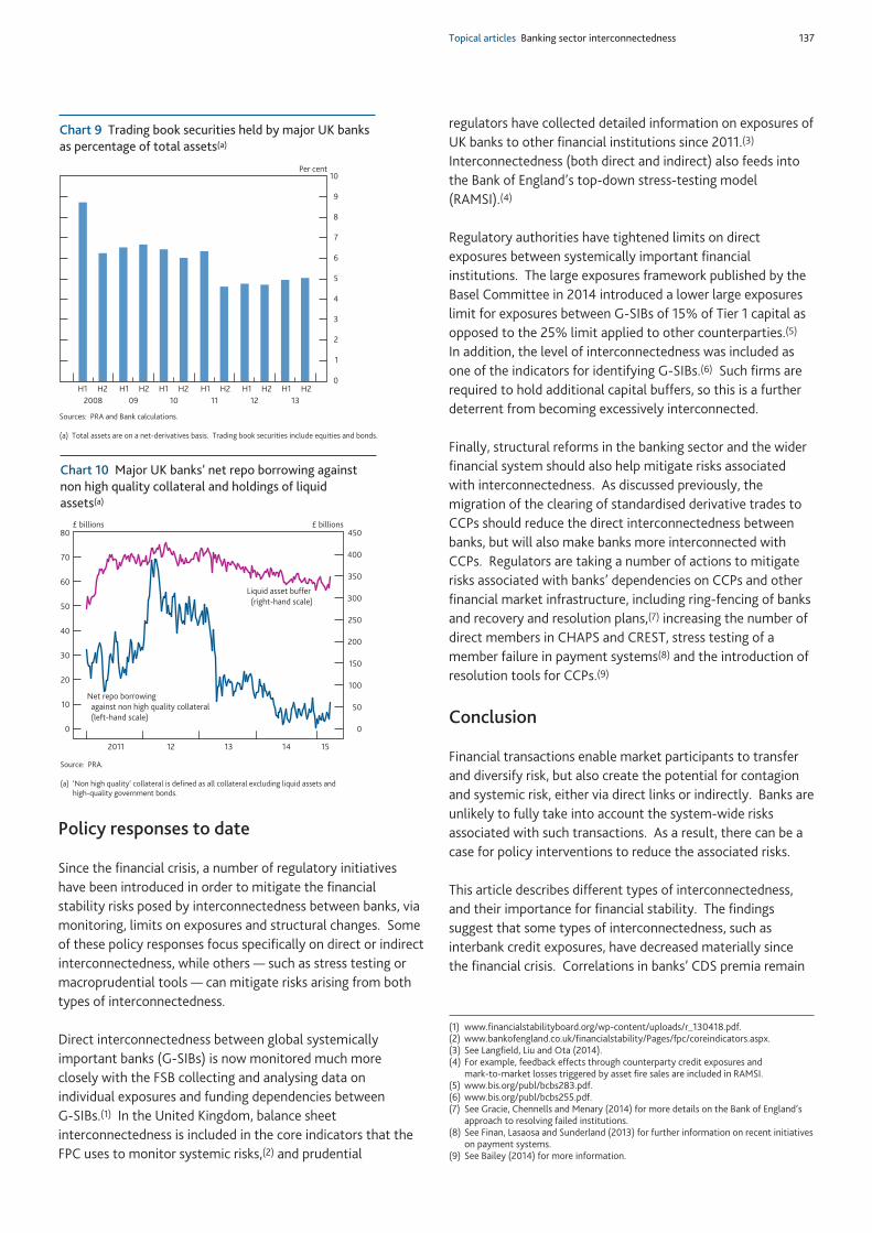
Topical articles Banking sector interconnectedness 137
Policy responses to date
Since the financial crisis, a number of regulatory initiativeshave been introduced in order to mitigate the financialstability risks posed by interconnectedness between banks, viamonitoring, limits on exposures and structural changes. Someof these policy responses focus specifically on direct or indirectinterconnectedness, while others — such as stress testing ormacroprudential tools — can mitigate risks arising from bothtypes of interconnectedness.
Direct interconnectedness between global systemicallyimportant banks (G-SIBs) is now monitored much moreclosely with the FSB collecting and analysing data onindividual exposures and funding dependencies betweenG-SIBs.(1) In the United Kingdom, balance sheetinterconnectedness is included in the core indicators that theFPC uses to monitor systemic risks,(2) and prudential
regulators have collected detailed information on exposures ofUK banks to other financial institutions since 2011.(3)
Interconnectedness (both direct and indirect) also feeds intothe Bank of England’s top-down stress-testing model(RAMSI).(4)
Regulatory authorities have tightened limits on directexposures between systemically important financialinstitutions. The large exposures framework published by theBasel Committee in 2014 introduced a lower large exposureslimit for exposures between G-SIBs of 15% of Tier 1 capital asopposed to the 25% limit applied to other counterparties.(5)
In addition, the level of interconnectedness was included asone of the indicators for identifying G-SIBs.(6) Such firms arerequired to hold additional capital buffers, so this is a furtherdeterrent from becoming excessively interconnected.
Finally, structural reforms in the banking sector and the widerfinancial system should also help mitigate risks associatedwith interconnectedness. As discussed previously, themigration of the clearing of standardised derivative trades toCCPs should reduce the direct interconnectedness betweenbanks, but will also make banks more interconnected withCCPs. Regulators are taking a number of actions to mitigaterisks associated with banks’ dependencies on CCPs and otherfinancial market infrastructure, including ring-fencing of banksand recovery and resolution plans,(7) increasing the number ofdirect members in CHAPS and CREST, stress testing of amember failure in payment systems(8) and the introduction ofresolution tools for CCPs.(9)
Conclusion
Financial transactions enable market participants to transferand diversify risk, but also create the potential for contagionand systemic risk, either via direct links or indirectly. Banks areunlikely to fully take into account the system-wide risksassociated with such transactions. As a result, there can be acase for policy interventions to reduce the associated risks.
This article describes different types of interconnectedness,and their importance for financial stability. The findingssuggest that some types of interconnectedness, such asinterbank credit exposures, have decreased materially sincethe financial crisis. Correlations in banks’ CDS premia remain
0
1
2
3
4
5
6
7
8
9
10
2008 09 10 11 12 13
Per cent
H1 H2 H1 H2 H1 H2 H1 H2 H1 H2 H1 H2
Sources: PRA and Bank calculations.
(a) Total assets are on a net-derivatives basis. Trading book securities include equities and bonds.
Chart 9 Trading book securities held by major UK banksas percentage of total assets(a)
0
50
100
150
200
250
300
350
400
450
0
10
20
30
40
50
60
70
80
2011 12 13 14 15
Net repo borrowing against non high quality collateral (left-hand scale)
Liquid asset buffer (right-hand scale)
£ billions £ billions
Source: PRA.
(a) ‘Non high quality’ collateral is defined as all collateral excluding liquid assets andhigh-quality government bonds.
Chart 10 Major UK banks’ net repo borrowing againstnon high quality collateral and holdings of liquidassets(a)
(1) www.financialstabilityboard.org/wp-content/uploads/r_130418.pdf. (2) www.bankofengland.co.uk/financialstability/Pages/fpc/coreindicators.aspx. (3) See Langfield, Liu and Ota (2014).(4) For example, feedback effects through counterparty credit exposures and
mark-to-market losses triggered by asset fire sales are included in RAMSI.(5) www.bis.org/publ/bcbs283.pdf. (6) www.bis.org/publ/bcbs255.pdf.(7) See Gracie, Chennells and Menary (2014) for more details on the Bank of England’s
approach to resolving failed institutions.(8) See Finan, Lasaosa and Sunderland (2013) for further information on recent initiatives
on payment systems.(9) See Bailey (2014) for more information.

138 Quarterly Bulletin 2015 Q2
elevated relative to pre-crisis, which may reflect higherindirect interconnectedness, but is more likely to be driven bycommon shocks.
This article has focused on interconnections between banks.The interconnectedness between banks and non-banks, as
well as between non-banks, is beyond the scope of this article,but is important for financial stability given the growingimportance of non-banks in the financial system. At present,sufficiently granular data to asses such risks is much morelimited.
References
Acharya, A and Yorulmazer, T (2008), ‘Information contagion and bank herding’, Journal of Money, Credit and Banking, Vol. 40, No. 1,pages 215–31.
Adrian, T and Shin, H (2008), ‘Liquidity and leverage’, Federal Reserve Bank of New York Staff Report No. 328.
Bailey, D (2014), ‘The Bank of England’s perspective on CCP risk management, recovery and resolution arrangements’, available atwww.bankofengland.co.uk/publications/Documents/speeches/2014/speech781.pdf.
Balluck, K (2015), ‘Investment banking: linkages to the real economy and the financial system’, Bank of England Quarterly Bulletin, Vol. 55,No. 1, pages 4–22, available at www.bankofengland.co.uk/publications/Documents/quarterlybulletin/2015/q101.pdf.
Farag, M, Harland, D and Nixon, D (2013), ‘Bank capital and liquidity’, Bank of England Quarterly Bulletin, Vol. 53. No. 3, pages 201–15,available at www.bankofengland.co.uk/publications/Documents/quarterlybulletin/2013/qb130302.pdf.
Finan, K, Lasaosa, A and Sunderland, J (2013), ‘Tiering in CHAPS’, Bank of England Quarterly Bulletin, Vol. 53, No. 4, pages 371–78, available atwww.bankofengland.co.uk/publications/Documents/quarterlybulletin/2013/qb130408.pdf.
Gorton, G and Metrick, A (2012), ‘Securitized banking and the run on repo’, Journal of Financial Economics, Vol. 104, No. 3, pages 425–51.
Gracie, A, Chennells, L and Menary, M (2014), ‘The Bank of England’s approach to resolving failed institutions’, Bank of England QuarterlyBulletin, Vol. 54, No. 4, pages 409–18, available at www.bankofengland.co.uk/publications/Documents/quarterlybulletin/2014/qb14q404.pdf.
Haldane, A (2009), ‘Rethinking the financial network’, available at www.bankofengland.co.uk/archive/Documents/historicpubs/speeches/2009/speech386.pdf.
Hull, J C (2008), Options, futures and other derivatives, 7th edition, Prentice-Hall.
IMF, BIS and FSB (2009), ‘Guidance to assess the systemic importance of financial institutions, markets and instruments: initial considerations’,report to G20 Finance Ministers and Governors.
Langfield, S, Liu, Z and Ota, T (2014), ‘Mapping the UK interbank system’, Bank of England Working Paper No. 516, available atwww.bankofengland.co.uk/research/Documents/workingpapers/2014/wp516.pdf.
Rehlon, A and Nixon, D (2013), ‘Central counterparties: what are they, why do they matter and how does the Bank supervise them?’, Bank ofEngland Quarterly Bulletin, Vol. 53, No. 2, pages 147–56, available at www.bankofengland.co.uk/publications/Documents/quarterlybulletin/2013/qb130206.pdf.
Scott, H S (2012), ‘Interconnectedness and contagion’, American Enterprise Institute Committee on Capital Market Regulation.
Upper, C (2010), ‘Simulation methods to assess the danger of contagion in interbank markets’, Journal of Financial Stability, Vol. 7, No. 3,pages 111–25.

Topical articles The prudential regulation of insurers under Solvency II 139
• Solvency II is a new regime for the prudential regulation of European insurance companies thatwill come into force on 1 January 2016.
• It will modernise the existing regulatory framework, with the objective of providing an enhancedand more consistent level of protection for policyholders across Europe.
• Solvency II introduces features to improve a firm’s understanding and management of its risks,which should result in improved resilience to shocks.
The prudential regulation of insurersunder Solvency IIBy Robin Swain and David Swallow of the Bank’s Prudential Policy Directorate.(1)
(1) The authors would like to thank Ishtiaq Faiz for his help in producing this article.
Overview
Insurance companies play a key role in the economy,allowing businesses and individuals to exchange the risk ofan uncertain and costly financial outcome for a fixed cost orpremium. The failure of a large insurance company coulddisrupt the broader provision of financial services, causingstress to spread throughout the financial system and realeconomy. Therefore, insurance companies need to besufficiently well-capitalised and prudently managed sothat they can withstand shocks.
European legislation for the prudential regulation ofinsurance companies has existed since the 1970s. There havebeen several limited reforms to this legislation but the latest,Solvency II, represents a fundamental modernisation ofEuropean insurance regulation. The main purpose ofSolvency II is to enhance the level of policyholder protectionacross Europe. The new regime should also improve theresilience of the insurance sector to shocks and so reduce theprobability of insurers failing.
Some of the key features that will be introduced are listed onthe summary table. Solvency II will require firms to identify,quantify and manage their risks on a forward-looking basis,while providing greater transparency to markets andsupervisors. The new regime will harmonise what has, overtime, become an increasingly fragmented regulatoryframework. A more harmonised framework should allowEuropean insurers to compete more effectively and reduceso-called ‘regulatory arbitrage’.
Due to the scale of reform, a number of measures are beingput in place to help firms manage the transition toSolvency II. In many respects, UK insurance companiesshould be better prepared for this transition as they alreadyneed to meet specific requirements under the currentUK regime that are based on similar principles to those ofSolvency II.
The Bank will monitor the effects of implementingSolvency II to ensure that gaps in the regulatory frameworkdo not emerge. It will also actively participate in futurepolicy debates as views and analysis develop further.
Click here for a short video that discusses some of the keytopics from this article.
Summary table Key features of Solvency II
Aspect of business or Change under Solvency IIsupervision
Accounting practices Market-consistent valuations introduced to provide firms with useful information for effective risk management.Quality of capital Enhanced to improve the ability of capital to absorb losses in times of financial difficulty.Capital requirements Forward-looking, risk-based capital requirements introduced to improve a firm’s resilience to financial shocks.Governance and risk Improved so that a firm should be better equipped to management requirements identify, manage and mitigate the risks that it is exposed to.Group supervision A rigorous, consistent approach to group supervision introduced to help supervisors understand all the risks that a firm within a group is exposed to.Market disclosures and Improved disclosures and reporting intended toreporting strengthen market discipline and to provide supervisors with better and more consistent information.
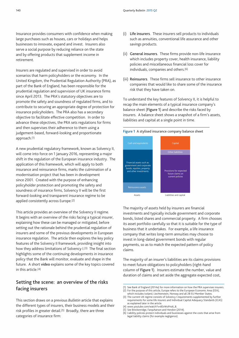
140 Quarterly Bulletin 2015 Q2
Insurance provides consumers with confidence when makinglarge purchases such as houses, cars or holidays and helpsbusinesses to innovate, expand and invest. Insurers alsoserve a social purpose by reducing reliance on the stateand by offering products that supplement income inretirement.
Insurers are regulated and supervised in order to avoidscenarios that harm policyholders or the economy. In theUnited Kingdom, the Prudential Regulation Authority (PRA), aspart of the Bank of England, has been responsible for theprudential regulation and supervision of UK insurance firmssince April 2013. The PRA’s statutory objectives are topromote the safety and soundness of regulated firms, and tocontribute to securing an appropriate degree of protection forinsurance policyholders. The PRA also has a secondaryobjective to facilitate effective competition. In order toadvance these objectives, the PRA sets regulations for firmsand then supervises their adherence to them using ajudgement-based, forward-looking and proportionateapproach.(1)
A new prudential regulatory framework, known as Solvency II,will come into force on 1 January 2016, representing a majorshift in the regulation of the European insurance industry. Theapplication of this framework, which will apply to bothinsurance and reinsurance firms, marks the culmination of amodernisation project that has been in developmentsince 2001. Created with the purpose of enhancingpolicyholder protection and promoting the safety andsoundness of insurance firms, Solvency II will be the firstforward-looking and transparent insurance regime to beapplied consistently across Europe.(2)
This article provides an overview of the Solvency II regime.It begins with an overview of the risks facing a typical insurer,explaining how these can be managed or mitigated, beforesetting out the rationale behind the prudential regulation ofinsurers and some of the previous developments in Europeaninsurance regulation. The article then explores the key policyfeatures of the Solvency II framework, providing insight intohow they address limitations of Solvency I.(3) The final sectionhighlights some of the continuing developments in insurancepolicy that the Bank will monitor, evaluate and shape in thefuture. A short video explains some of the key topics coveredin this article.(4)
Setting the scene: an overview of the risksfacing insurers
This section draws on a previous Bulletin article that explainsthe different types of insurers, their business models and theirrisk profiles in greater detail.(5) Broadly, there are threecategories of insurance firm:
(i) Life insurers. These insurers sell products to individualssuch as annuities, conventional life assurance and othersavings products.
(ii) General insurers. These firms provide non-life insurancewhich includes property cover, health insurance, liabilitypolicies and miscellaneous financial loss cover forindividuals, companies and others.(6)
(iii) Reinsurers. These firms sell insurance to other insurancecompanies that would like to share some of the insurancerisk that they have taken on.
To understand the key features of Solvency II, it is helpful torecap the main elements of a typical insurance company’sbalance sheet (Figure 1) and describe the risks faced byinsurers. A balance sheet shows a snapshot of a firm’s assets,liabilities and capital at a single point in time.
The majority of assets held by insurers are financialinvestments and typically include government and corporatebonds, listed shares and commercial property. A firm choosesits asset portfolio carefully so that it is suitable for the type ofbusiness that it undertakes. For example, a life insurancecompany that writes long-term annuities may choose toinvest in long-dated government bonds with regularpayments, so as to match the expected pattern of policyclaims.
The majority of an insurer’s liabilities are its claims provisionsto meet future obligations to policyholders (right-handcolumn of Figure 1). Insurers estimate the number, value andduration of claims and set aside the aggregate expected cost,
(1) See Bank of England (2014a) for more information on how the PRA supervises insurers.(2) For the purpose of this article, Europe refers to the European Economic Area (EEA),
which includes Iceland, Liechtenstein, Norway and all 28 EU Member States.(3) The current UK regime consists of Solvency I requirements supplemented by further
requirements for some life insurers and Individual Capital Adequacy Standards (ICAS)as explained later in the article.
(4) www.youtube.com/watch?v=8SrWoPns6_8.(5) See Breckenridge, Farquharson and Hendon (2014).(6) Liability policies protect individuals and businesses against the costs that arise from
legal liability claims (for example negligence).
Cash and equivalents
Financial assets such as:government and corporatebonds, equities, property
and other investments
Reinsurance assets
Capital
Other liabilities
Provisions for expectedfuture claims oncurrent policies
Liabilities and capitalAssets
Figure 1 A stylised insurance company balance sheet
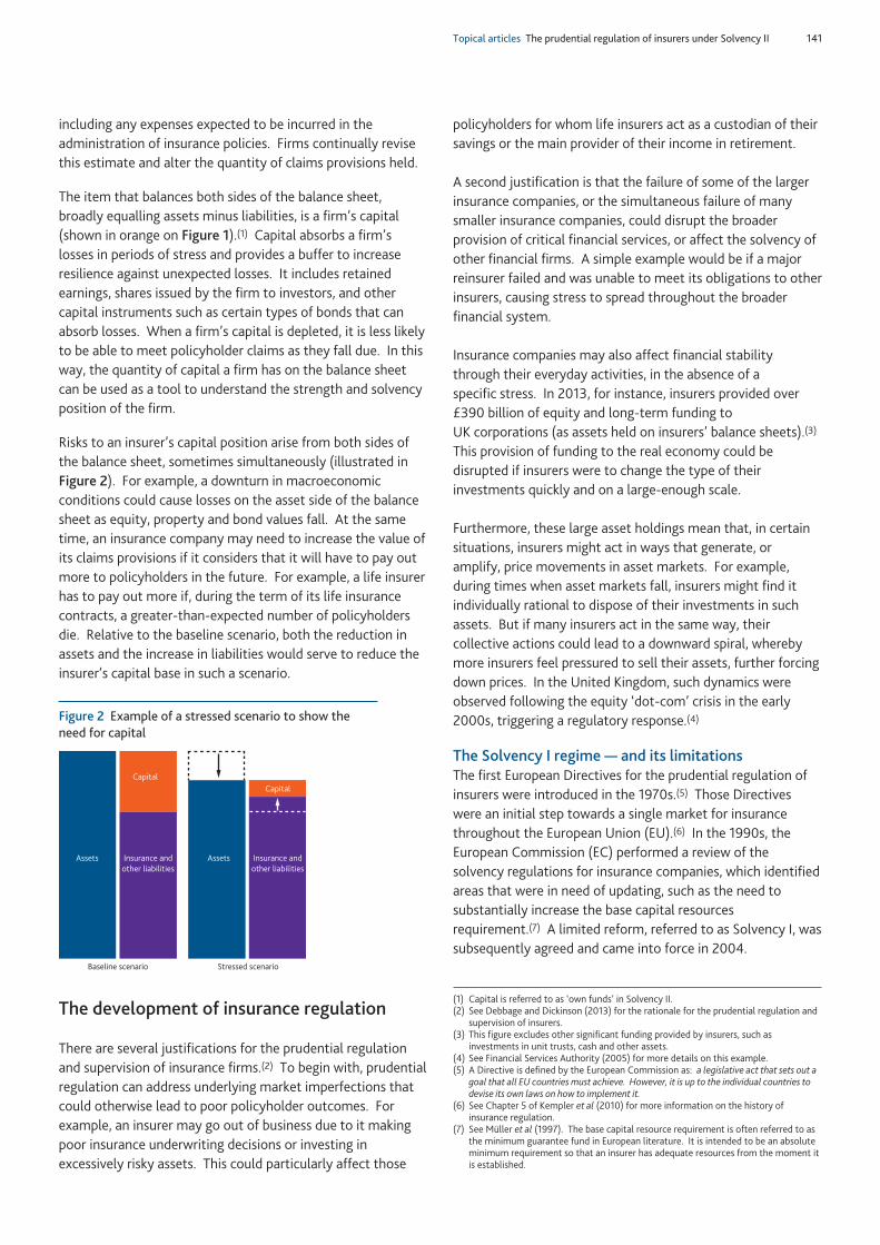
Topical articles The prudential regulation of insurers under Solvency II 141
including any expenses expected to be incurred in theadministration of insurance policies. Firms continually revisethis estimate and alter the quantity of claims provisions held.
The item that balances both sides of the balance sheet,broadly equalling assets minus liabilities, is a firm’s capital(shown in orange on Figure 1).(1) Capital absorbs a firm’slosses in periods of stress and provides a buffer to increaseresilience against unexpected losses. It includes retainedearnings, shares issued by the firm to investors, and othercapital instruments such as certain types of bonds that canabsorb losses. When a firm’s capital is depleted, it is less likelyto be able to meet policyholder claims as they fall due. In thisway, the quantity of capital a firm has on the balance sheetcan be used as a tool to understand the strength and solvencyposition of the firm.
Risks to an insurer’s capital position arise from both sides ofthe balance sheet, sometimes simultaneously (illustrated inFigure 2). For example, a downturn in macroeconomicconditions could cause losses on the asset side of the balancesheet as equity, property and bond values fall. At the sametime, an insurance company may need to increase the value ofits claims provisions if it considers that it will have to pay outmore to policyholders in the future. For example, a life insurerhas to pay out more if, during the term of its life insurancecontracts, a greater-than-expected number of policyholdersdie. Relative to the baseline scenario, both the reduction inassets and the increase in liabilities would serve to reduce theinsurer’s capital base in such a scenario.
The development of insurance regulation
There are several justifications for the prudential regulationand supervision of insurance firms.(2) To begin with, prudentialregulation can address underlying market imperfections thatcould otherwise lead to poor policyholder outcomes. Forexample, an insurer may go out of business due to it makingpoor insurance underwriting decisions or investing inexcessively risky assets. This could particularly affect those
policyholders for whom life insurers act as a custodian of theirsavings or the main provider of their income in retirement.
A second justification is that the failure of some of the largerinsurance companies, or the simultaneous failure of manysmaller insurance companies, could disrupt the broaderprovision of critical financial services, or affect the solvency ofother financial firms. A simple example would be if a majorreinsurer failed and was unable to meet its obligations to otherinsurers, causing stress to spread throughout the broaderfinancial system.
Insurance companies may also affect financial stabilitythrough their everyday activities, in the absence of aspecific stress. In 2013, for instance, insurers provided over£390 billion of equity and long-term funding toUK corporations (as assets held on insurers’ balance sheets).(3)
This provision of funding to the real economy could bedisrupted if insurers were to change the type of theirinvestments quickly and on a large-enough scale.
Furthermore, these large asset holdings mean that, in certainsituations, insurers might act in ways that generate, oramplify, price movements in asset markets. For example,during times when asset markets fall, insurers might find itindividually rational to dispose of their investments in suchassets. But if many insurers act in the same way, theircollective actions could lead to a downward spiral, wherebymore insurers feel pressured to sell their assets, further forcingdown prices. In the United Kingdom, such dynamics wereobserved following the equity ‘dot-com’ crisis in the early2000s, triggering a regulatory response.(4)
The Solvency I regime — and its limitationsThe first European Directives for the prudential regulation ofinsurers were introduced in the 1970s.(5) Those Directiveswere an initial step towards a single market for insurancethroughout the European Union (EU).(6) In the 1990s, theEuropean Commission (EC) performed a review of thesolvency regulations for insurance companies, which identifiedareas that were in need of updating, such as the need tosubstantially increase the base capital resourcesrequirement.(7) A limited reform, referred to as Solvency I, wassubsequently agreed and came into force in 2004.
(1) Capital is referred to as ‘own funds’ in Solvency II.(2) See Debbage and Dickinson (2013) for the rationale for the prudential regulation and
supervision of insurers.(3) This figure excludes other significant funding provided by insurers, such as
investments in unit trusts, cash and other assets.(4) See Financial Services Authority (2005) for more details on this example.(5) A Directive is defined by the European Commission as: a legislative act that sets out a
goal that all EU countries must achieve. However, it is up to the individual countries todevise its own laws on how to implement it.
(6) See Chapter 5 of Kempler et al (2010) for more information on the history ofinsurance regulation.
(7) See Müller et al (1997). The base capital resource requirement is often referred to asthe minimum guarantee fund in European literature. It is intended to be an absoluteminimum requirement so that an insurer has adequate resources from the moment itis established.
Assets
Stressed scenarioBaseline scenario
Capital
Insurance andother liabilities
Capital
Insurance andother liabilities
Assets
Figure 2 Example of a stressed scenario to show theneed for capital
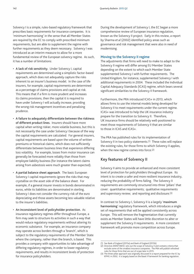
142 Quarterly Bulletin 2015 Q2
Solvency I is a simple, rules-based regulatory framework thatprescribes basic requirements for insurance companies. It is‘minimum harmonising’ in the sense that all Member Statesare required by the EC to comply with prescribed minimumrequirements, but are able to supplement the regime withfurther requirements as they deem necessary. Solvency I wasintroduced as an interim measure to allow for a morefundamental review of the European solvency regime. As such,it has a number of limitations:
• A lack of risk sensitivity. Under Solvency I, capitalrequirements are determined using a simplistic factor-basedapproach, which does not adequately capture the risksinherent to an insurer’s business model. In the case of lifeinsurers, for example, capital requirements are determinedas a percentage of claims provisions and capital at risk.This means that if a firm is more prudent and increasesits claims provisions, then the capital it is required tohave under Solvency I will actually increase, providingthe wrong risk management incentives and penalising prudence.
• A failure to adequately differentiate between the riskinessof different product lines. Insurers should have morecapital when writing riskier, more volatile business, but this isnot necessarily the case under Solvency I because of the waythe capital requirements are calculated. For general insurers,capital requirements are based upon the volume of writtenpremiums or historical claims, which does not sufficientlydifferentiate between business lines that experience differingloss volatility. For example, losses from motor insurance cangenerally be forecasted more reliably than those fromemployee liability business (for instance the latent claimsarising from asbestosis were much greater than expected).
• A partial balance sheet approach. The basic EuropeanSolvency I capital requirements ignore the risks that maycrystallise on the asset side of the balance sheet. Forexample, if a general insurer invests in bonds denominated ineuros, while its liabilities are denominated in sterling,Solvency I does not consider the currency risk of the eurodepreciating and those assets becoming less valuable relativeto the insurer’s liabilities.
• An inconsistent level of policyholder protection. Asinsurance regulatory regimes differ throughout Europe, afirm may seek to structure its activities in such a way thatwould reduce regulatory requirements without altering itseconomic substance. For example, an insurance companymay operate across borders through a ‘branch’, which issubject to the regulatory requirements of the Member Statewhere the company, rather than the branch, is based. Thisprovides a company with opportunities to take advantage ofdiffering regulatory regimes, in order to lower regulatoryrequirements, and results in inconsistent levels of protectionfor insurance policyholders.
During the development of Solvency I, the EC began a morecomprehensive review of European insurance regulation,known as the Solvency II project. Early in this review, a reportby Sharma et al (2002) identified policy areas such asgovernance and risk management that were also in need ofmodernising.
Moving to the Solvency II regimeThe adjustments that firms will need to make to adapt to theSolvency II regime will differ among EU Member Statesdepending on the extent to which each Member Statesupplemented Solvency I with further requirements. TheUnited Kingdom, for instance, supplemented Solvency I withadditional requirements in 2004. These included the IndividualCapital Adequacy Standards (ICAS) regime, which bears severalsignificant similarities to the Solvency II framework.
Furthermore, the PRA introduced ICAS+ in 2013, whichallows firms to use the internal models being developed forSolvency II to meet requirements under the current regime.ICAS+ was introduced to help the UK insurance industryprepare for the transition to Solvency II. Therefore,UK insurance firms should be relatively well-positioned tomeet those requirements of Solvency II that are similarto those in ICAS and ICAS+.
The PRA has published rules for its implementation ofSolvency II in two policy statements.(1) These rules will replacethe existing rules, for those firms to which Solvency II applies,when the new regime comes into force.(2)
Key features of Solvency II
Solvency II aims to provide an enhanced and more consistentlevel of protection for policyholders throughout Europe. Itsintent is to create a safer and more resilient insurance industry,reducing the probability of firms failing. The Solvency IIrequirements are commonly structured into three ‘pillars’ thatcover: quantitative requirements; qualitative requirementsand supervisory review; and reporting and disclosure.(3)
In contrast to Solvency I, Solvency II is a largely ‘maximumharmonising’ regulatory framework, which introduces a singleset of requirements that will be applied consistently acrossEurope. This will remove the fragmentation that currentlyexists as Member States will have little discretion to alter orsupplement the Solvency II requirements. A more consistentframework will promote more competition across Europe.
(1) See Bank of England (2015a) and Bank of England (2015b).(2) Directive 2009/138/EC sets out the scope of Solvency II and contains criteria that
exclude some of the smallest insurance companies. The PRA will publish refreshedrules for those firms that are out of scope later in 2015.
(3) The three-pillar approach was originally discussed in a report prepared for the EC byKPMG in 2002; it is largely based on the Basel II framework for banking regulation.

Topical articles The prudential regulation of insurers under Solvency II 143
Solvency II adopts a ‘total balance sheet’ approach: the risksto assets, liabilities and the interactions between them need tobe considered in setting capital requirements. Furthermore, itintroduces several key features, some of which seek to ensurethat firms identify, quantify and manage their risks on aproportionate and forward-looking basis. Other features willprovide greater transparency to markets and supervisors. Inparticular, Solvency II introduces:
• market-consistent valuation of assets and liabilities;
• enhanced quality of capital;
• a forward-looking and risk-based approach to setting capitalrequirements;
• improved governance and risk management requirements;
• a rigorous approach to group supervision; and
• strengthened market discipline through firm disclosures.
The rest of this section considers and explains each of thesefeatures in turn.
Market-consistent valuation of assets and liabilitiesSolvency II introduces a new basis of preparation for aninsurance company’s balance sheet (as shown in Figure 3),which is based on the principle of market-consistentvaluations. Essentially, this means that the value of assets andliabilities reflect the current value at which they could betraded in financial markets, rather than their originalaccounting value. In 2004, the United Kingdom introducedsimilar valuation methods as part of the ICAS framework.
A simple example illustrates the advantages of this approach.Suppose an insurer has invested £100 million in propertyassets but that, following a downturn in the property market,these assets could only be sold for £70 million. If changes in
value such as this are not reflected in asset prices on thebalance sheet, it may give a false impression of a firm’ssolvency and supervisors would be unable to assess accuratelythe safety and soundness of the insurer.
Different approaches are required to determinemarket-consistent values of an insurance company’s assetsand liabilities. Many assets are traded in sufficiently deep andliquid markets that provide readily available prices, which aregenerally taken to be market values. No such marketgenerally exists for insurance liabilities, which are specific tothe contract between the firm and the policyholder.(1)
Solvency II’s interpretation of the market value of insuranceliabilities requires insurers to forecast expected future liabilitycash flows and then discount them using risk-free interestrates of an appropriate maturity, to arrive at a ‘bestestimate’.(2) A ‘risk margin’ is added to this best estimate inorder to produce a market-consistent value.(3) This isexplained further in the box on page 144.
Market-consistent valuations are important as they ensurethat short-term asset price changes that may affect a firm’ssolvency are reflected on the balance sheet. However, aninsurer with long-term liabilities that holds long-term assetsto maturity, in order to pay policyholder claims, is lessaffected by such short-term price changes. The ‘matchingadjustment’ (which is explained in Annex 2) is intended toaddress this issue. It is being introduced as part of thelong-term guarantees (LTG) package of Solvency II, whichincludes a number of measures intended to make the newregime appropriate for the provision of long-term insuranceproducts.(4) Other LTG measures include:
• The ‘volatility adjustment’, which is a countercyclicalmeasure intended to prevent investment behaviours thatamplify asset price movements. Broadly, it is expected towork by reducing the value of liabilities (below thatcalculated using a risk-free discount rate) in stressedscenarios.
• An agreed method for the ‘extrapolation of the risk-freerate’ to determine long-term discount rates where there isno reliable market data.
• Transitional measures, which include the ‘transitionaldeduction from technical provisions’, which will help firmstransition to the new ‘going-concern’ regime. This isexplained in the box on page 144.
Market value of assets
Reinsurance assets(a)
Surplus capital
Risk margin
Best estimate of liabilities
Liabilities and capitalAssets
Regulatory capital(b)
(a) Reinsurance assets are calculated on a best-estimate basis.(b) This is qualifying capital that satisfies regulatory requirements.
Figure 3 Stylised example of an insurer’s balance sheetunder Solvency II
(1) Insurance liabilities are known as ‘technical provisions’ in Solvency II.(2) The ‘best estimate’ is a firm’s forecast of the cash flows that are most likely to occur,
rather than, for example, the forecast of the most profitable or most prudent scenarios.(3) This approach to determine the market-consistent valuation of insurance liabilities
applies to insurance liabilities that cannot be reliably replicated by the cash flows offinancial instruments with observable market values. Otherwise, the market value ofliabilities that can be replicated, such as the value of some guarantees in life insurancecontracts, should be determined from the market value of the replicating financialinstruments.
(4) This package was agreed as part of Directive 2014/51/EU.

144 Quarterly Bulletin 2015 Q2
Transitioning to a ‘going-concern’ regime
Solvency I can be considered as a ‘gone-concern’ regime. Afirm is required to calculate financial requirements under theassumption that it writes no new business in the future andthat it will ‘run-off’ its existing business over time.(1) The mainlimitation of this approach is that it is unrealistic to assumethat all insurance firms will simultaneously stop writing newbusiness.
Solvency II takes a different view of the insurance industry byconsidering firms as ‘going concerns’. Under this approach,insurers will determine their financial requirements under theassumption that they will continue to operate and write newbusiness for the foreseeable future. This assumption isconsistent with the nature of risk management in Solvency II,which requires firms to identify and manage risks on acontinuing and forward-looking basis. A going-concernapproach should improve policyholder protection and betterreflects the realities of insurance business.
The going-concern regime seeks to ensure that if a firm doesgo out of business, policyholder protection and continuity ofinsurance cover are sustained. To achieve this, Solvency IIintroduces the ‘risk margin’: a provision that increases thebest estimate of a firm’s insurance liabilities to produce amarket-consistent value (as shown in Figure 3). Therefore, therisk margin will enable an insurance company that cannotcontinue in business to transfer its commitments to anothercompany that is able to fulfil those obligations, therebyprotecting policyholders. The risk margin is fundamentallydifferent to the company-specific prudential margins requiredby Solvency I (explained in Annex 1) and will promoteconsistency and transparency across the industry.
Solvency II contains a number of transitional measures, whichare an important feature of the implementation of any new
regulatory regime. These measures should help firms adjust tothe new framework by limiting any disruption and addressingany unintended consequences of adjusting to Solvency II.Firms’ use of transitional measures will be publicly disclosedunder Solvency II, reinforcing transparency in the market andpromoting greater comparability between insurers acrossEurope.
The ‘transitional deduction from technical provisions’ is oneexample of a transitional measure in the LTG package.(2) Dueto the move to a going-concern regime, Solvency II willultimately require some firms to hold a greater quantity ofclaims provisions compared to the current regime. For firmswhere this is the case, and subject to supervisory approval,firms will be able to use this transitional measure to increasethe quantity of their provisions gradually over 16 years, fromthe current level to that required under Solvency II. Thetransitional deduction is subject to a safeguard so that a firm’soverall financial resources (claims provisions and capital) donot fall below what they are under the current regime. Thisensures that use of the transitional measure does not lead to adecrease in protection for policyholders.
Insurance contracts that were written before the applicationof Solvency II will expire over time. This will remove the needfor firms to bridge the entire gap in claims provisions betweenSolvency I and Solvency II. New business written after thecommencement of Solvency II should not need the benefits oftransitional measures because it should be compatible withthe full requirements of the new regime.
Enhanced quality of capitalEven if the quantity of capital held by an insurance firm isconsidered to be sufficient, if that capital is not of anappropriate quality then it may not be able to absorb losseseffectively. Recent thinking on the relative qualities ofcapital has been driven by the experience of the bankingsector in the financial crisis. It has become clear that agreater emphasis needs to be placed on the highest qualityof capital.
Solvency II classifies different forms of capital into three ‘tiers’which, broadly speaking, separate capital based on its abilityto absorb losses.(1) Tier 1 capital, such as common equity andretained earnings, is the highest quality of capital and must beable to absorb losses on a day-to-day, ‘going-concern’ basis.
Tier 2 capital, such as subordinated debt, is of a lower qualityand only needs to absorb losses on insolvency. Finally, Tier 3capital is the lowest quality of capital permitted and has onlylimited loss-absorbing capacity. It is unlikely that significantquantities of Tier 3 capital will be issued by firms underSolvency II.
Solvency II introduces significant measures to improve thequality of capital held by insurance firms, some of which areexplained in Figure 4.(2)
(1) Once entering the run-off process, a firm will continue to operate in order to meetthe obligations of existing contracts up until their expiration. This period couldextend for 30–40 years for those insurers that sell long-term policies, such as lifeinsurance.
(2) See HM Treasury (2015) for the Solvency II Directive’s provisions on this transitionalmeasure.
(1) While different to the tiers of Solvency II, the United Kingdom introduced tiers fordifferent quality capital instruments as an additional requirement to Solvency I.
(2) See Bank of England (2015a). PRA Supervisory Statement 3/15, ‘The quality of capitalinstruments’ is part of this policy statement and gives more information. The PRARulebook contains the relevant rules.

Topical articles The prudential regulation of insurers under Solvency II 145
While improving the quality of capital is fundamental toSolvency II, the framework recognises that insurers cannotchange all of their capital instruments to comply withSolvency II requirements overnight. For instance, many firmshave issued long-dated or perpetual capital instruments beforethe commencement of Solvency II. Transitional measureshave therefore been put in place, allowing firms up toten years to replace capital instruments that are not compliantwith Solvency II requirements.
Forward-looking, risk-based capital requirementsIn contrast to Solvency I, Solvency II introducesforward-looking, risk-based capital requirements that provideincentives for firms to improve their understanding of, and tomanage better, the risks that they face. Capital requirementsshould consider all risks to which firms are exposed. TheSolvency II capital requirements should improve the safetyand soundness of insurers across Europe.
Two capital requirements are being introduced by Solvency II:the solvency capital requirement (SCR) and the minimumcapital requirement (MCR). The SCR is the quantity of capitalthat is intended to provide protection against unexpectedlosses, over the following year, up to the statistical level of a‘1 in 200-year event’. This is a robust requirement that isdesigned so that insurers should be able to withstand all butthe most severe of shocks. The MCR denotes a level belowwhich policyholders would be exposed to an unacceptablelevel of risk. Together, the SCR and MCR act as trigger pointsin the ‘supervisory ladder of intervention’ introduced bySolvency II, shown in Figure 5.
The majority of firms will calculate their SCR using a ‘standardformula’ — a standardised calculation intended to capture therisk profile of most European insurance firms. First, firms needto identify risks, such as market and insurance underwritingrisks, which are relevant to their business. A prescribedcalculation methodology is then used to determine thequantity of capital required to cover these risks.
Alternatively, firms may use an internal model to calculate theSCR. An internal model must be tailored to the specific riskprofile of a firm and is subject to prior supervisory approval toverify that it is robust and fit for purpose. Several tests and
standards are set out in Solvency II, which an internal modelneeds to satisfy, in order to gain regulatory approval. Theseinclude the ‘use test’, as well as further standards such as thestatistical quality, calibration, validation and documentationof the model.
The use test will be used to verify that internal models areemployed not just to satisfy the regulatory requirement ofcalculating the SCR, but as a tool that is part of a firm’s wider,risk management and decision-making processes. Forexample, suppose a general insurer writes household andtravel insurance. If it then considered a change of strategy andadditionally wanted to start writing motor insurance, the firmshould use its internal model to assess the risks of thisdecision. The use test also will examine the extent to whichan internal model is used and understood by a firm’smanagement and Board.
Improved governance and risk managementrequirementsThe recognition of the importance of good governancepractices was fundamental to the development of Solvency II.It is a policy area that the United Kingdom has long identifiedas an important part of a framework for prudential regulation.The report by Sharma et al (2002) identified a causalrelationship between firms that fail and those that areinherently vulnerable due to ‘underlying managementweakness or operational weakness’. Good governancepractices and strong risk management are therefore essentialaspects of a prudential regulatory framework.
Individuals that run insurance companies should have clearlydefined responsibilities and are expected to behave withhonesty, integrity and competence in order to provide soundand prudent management. For this purpose, the PRA isintroducing the senior insurance managers regime.(1) Thisenhances the current ‘fit and proper’ requirements and isintended to ensure the accountability of senior managementin the insurance sector.
Capital in excess of capital requirements
Supervisory ladder of interventionCapital
SCR
MCR
As capital falls
Firm breaches solvency capital requirement (SCR): it must consider and action a plan to restore its capital position and/or reduce its risk profile. Distributions to investors are either cancelled or deferred. The SCR acts as an intervention point for supervisors to take action.
Firm breaches minimum capital requirement (MCR): regulatory action is taken and the firm must submit a plan for approval, explaining how it will restore capital above the MCR within three months. If the firm is unable to do so, its authorisation may be withdrawn.
Figure 5 Supervisory ladder of intervention
(1) See Bank of England (2015b) for more information.
Full flexibility over payments to investors For Tier 1 capital, there should be no mandatory payments to investors. Depending on the capital instrument, declared payments should either be cancelled or deferred if they would cause a breach of capital requirements.
Effective loss absorbency High-quality Tier 1 capital must be able to absorb losses effectively — either automatically or through a mechanism to absorb losses when defined ‘trigger points’ are breached.
Capital composition limits Solvency II requires insurers to have sufficient quantities of high-quality capital and limits the amount that can be covered by low-quality capital.
Duration of capital Capital must have a sufficient duration to be reliably able to absorb losses when needed. Solvency II introduces strict requirements for those forms of capital that are not permanent.
Figure 4 Improvements to the quality of capital under Solvency II

146 Quarterly Bulletin 2015 Q2
Solvency II requires insurers to take a comprehensive approachto considering their risks through the own risk and solvencyassessment (ORSA). Regulatory capital requirements may notadequately capture some risks which are difficult to quantifyaccurately, such as cyber risk (which can be both a risk to theinsurer and an insured risk). Furthermore, firms face risks thatspan the entirety of their business plan, such as the long-termeffects of climate change, changes in which are not necessarilysignificant over the one-year time horizon used in thecalibration of the SCR. By requiring a firm’s management toconsider risks such as these, the ORSA should help firms tounderstand and manage all the risks they are exposed to.
Under Solvency II, insurance companies will have greaterflexibility in their investment decisions, as the existing crude,quantitative limitations over asset choice and compositionlimits will be removed. The ‘prudent person principle’ is anapproach to regulation that places responsibility forinvestment decisions on a firm’s management. The PRA willthen form judgements on the ability of a firm’s managementto identify, manage and mitigate investment risks.
A rigorous approach to group supervisionSometimes, an insurance group will have a complex structurethat consists of a mixture of regulated and non-regulatedentities that may operate across many different regulatoryjurisdictions (Figure 6). As a result, the overall group may beexposed to some risks that are not obvious or captured whenconsidering an individual insurance firm within the group.
Two examples of such risks are the so-called ‘double gearing’and ‘leveraging’ of capital. Double gearing occurs when firmsuse the same capital resource more than once within a groupto meet capital requirements. Leveraging of capital refers to asituation where capital instruments are passed down a groupand artificially ‘upgraded’ in quality. This can occur if aholding company issues a Tier 2 debt instrument and thenpasses down the proceeds to an individual insurance entitywithin the group as Tier 1 equity.
Solvency II looks to improve on the current approach to groupsupervision, introduced by the Insurance Groups Directive(IGD),(1) through the introduction of a more rigorous approach.The IGD is based on the concept that group supervision shouldsupplement the supervision of individual insurance entities.This concept remains fundamental to Solvency II and helps toprovide a more complete view of where the risks to theprudential soundness of individual insurance companies liewithin a group. Group supervision under Solvency II is not anattempt to prudentially supervise every firm within a group,for example, an ‘offshore oil company’ (given as an example ofa non-regulated entity in Figure 6) would not be supervised bythe PRA.
A key aspect of group supervision is determining a group’scapital resources and capital requirements, for which there aretwo approaches. The first involves consolidating the variousgroup entities onto one balance sheet and then calculating thegroup capital resources and SCR. A second approach is tocalculate the capital resources and capital requirements for allindividual entities and then add the figures to obtain theoverall figures for the group. Importantly, both of thesemethods require that any double use or upgrading of capital iseliminated in the group calculation. Solvency II also containsadditional governance and reporting requirements to facilitategroup supervision.
Market discipline through firm disclosuresSolvency II introduces new reporting and disclosurerequirements for firms, with the aim of improving theavailability of information to the market. Firms will berequired to publish a solvency and financial condition report(SFCR) annually and disclose additional information privatelyto regulators. In the SFCR, firms need to clearly explainaspects of their approach to Solvency II, such as the use of aninternal model and any non-compliance with regulatorysolvency requirements. Solvency II sets out the disclosurerequirements for the SFCR such that the quality andstandardisation of firm disclosures should improve.(2) Theimproved reporting requirements will also provide supervisorswith better and more consistent information.
The higher quality and quantity of firm disclosures, in turn,should improve market participants’ understanding of aninsurer’s business model and risks, thereby strengtheningmarket discipline. For example, firms will be required todisclose any significant non-compliance with the SCR, toexplain the causes and consequences of this non-compliance,and to disclose any measures taken to resolve the breach.
US-regulated
EEA-regulated
Non-regulated
Ultimate worldwideholding company
Holding company(UK)
Reinsurer(France)
Bank(UK)
Insurer(UK)
Holding company(Germany)
Insurer(Italy)
Insurer(Germany)
Reinsurer(US)
Offshore oilcompany
Figure 6 Stylised example of a group structure
(1) See Directive 98/78/EC for more information.(2) The structure and content of the SFCR can be found in Commission Delegated
Regulation (EU) 2015/35 (2014).
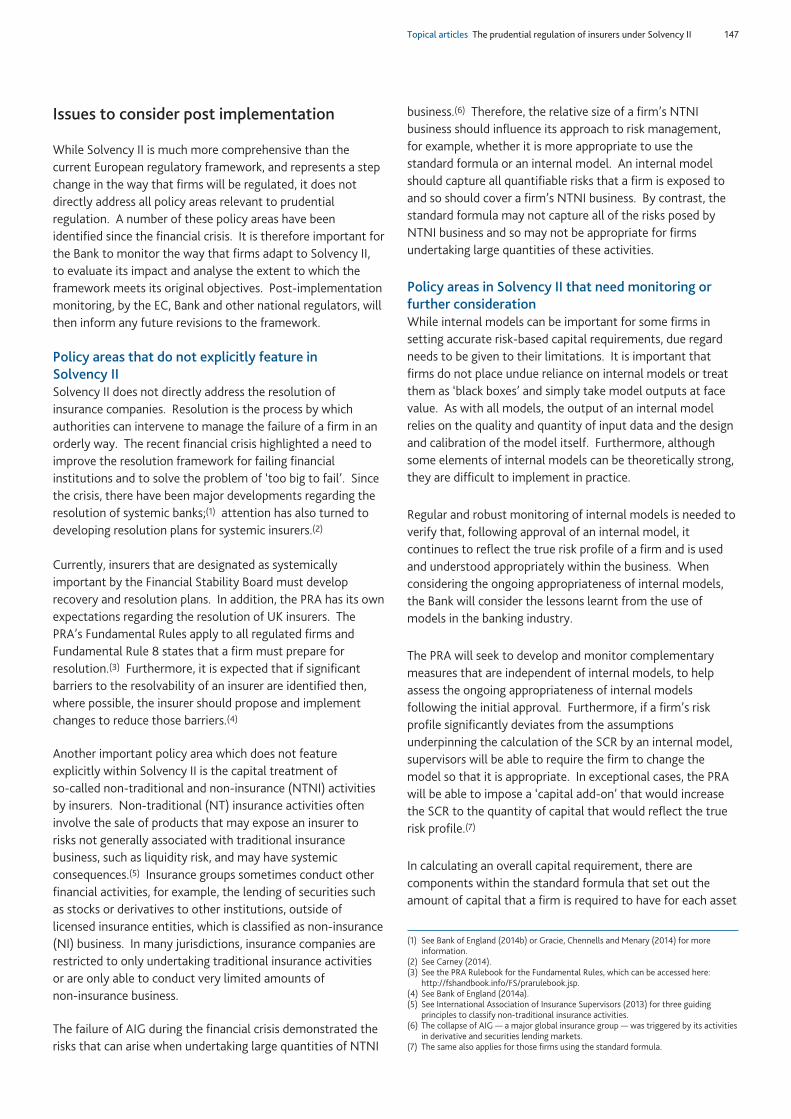
Topical articles The prudential regulation of insurers under Solvency II 147
Issues to consider post implementation
While Solvency II is much more comprehensive than thecurrent European regulatory framework, and represents a stepchange in the way that firms will be regulated, it does notdirectly address all policy areas relevant to prudentialregulation. A number of these policy areas have beenidentified since the financial crisis. It is therefore important forthe Bank to monitor the way that firms adapt to Solvency II,to evaluate its impact and analyse the extent to which theframework meets its original objectives. Post-implementationmonitoring, by the EC, Bank and other national regulators, willthen inform any future revisions to the framework.
Policy areas that do not explicitly feature inSolvency IISolvency II does not directly address the resolution ofinsurance companies. Resolution is the process by whichauthorities can intervene to manage the failure of a firm in anorderly way. The recent financial crisis highlighted a need toimprove the resolution framework for failing financialinstitutions and to solve the problem of ‘too big to fail’. Sincethe crisis, there have been major developments regarding theresolution of systemic banks;(1) attention has also turned todeveloping resolution plans for systemic insurers.(2)
Currently, insurers that are designated as systemicallyimportant by the Financial Stability Board must developrecovery and resolution plans. In addition, the PRA has its ownexpectations regarding the resolution of UK insurers. ThePRA’s Fundamental Rules apply to all regulated firms andFundamental Rule 8 states that a firm must prepare forresolution.(3) Furthermore, it is expected that if significantbarriers to the resolvability of an insurer are identified then,where possible, the insurer should propose and implementchanges to reduce those barriers.(4)
Another important policy area which does not featureexplicitly within Solvency II is the capital treatment ofso-called non-traditional and non-insurance (NTNI) activitiesby insurers. Non-traditional (NT) insurance activities ofteninvolve the sale of products that may expose an insurer torisks not generally associated with traditional insurancebusiness, such as liquidity risk, and may have systemicconsequences.(5) Insurance groups sometimes conduct otherfinancial activities, for example, the lending of securities suchas stocks or derivatives to other institutions, outside oflicensed insurance entities, which is classified as non-insurance(NI) business. In many jurisdictions, insurance companies arerestricted to only undertaking traditional insurance activitiesor are only able to conduct very limited amounts ofnon-insurance business.
The failure of AIG during the financial crisis demonstrated therisks that can arise when undertaking large quantities of NTNI
business.(6) Therefore, the relative size of a firm’s NTNIbusiness should influence its approach to risk management,for example, whether it is more appropriate to use thestandard formula or an internal model. An internal modelshould capture all quantifiable risks that a firm is exposed toand so should cover a firm’s NTNI business. By contrast, thestandard formula may not capture all of the risks posed byNTNI business and so may not be appropriate for firmsundertaking large quantities of these activities.
Policy areas in Solvency II that need monitoring orfurther consideration While internal models can be important for some firms insetting accurate risk-based capital requirements, due regardneeds to be given to their limitations. It is important thatfirms do not place undue reliance on internal models or treatthem as ‘black boxes’ and simply take model outputs at facevalue. As with all models, the output of an internal modelrelies on the quality and quantity of input data and the designand calibration of the model itself. Furthermore, althoughsome elements of internal models can be theoretically strong,they are difficult to implement in practice.
Regular and robust monitoring of internal models is needed toverify that, following approval of an internal model, itcontinues to reflect the true risk profile of a firm and is usedand understood appropriately within the business. Whenconsidering the ongoing appropriateness of internal models,the Bank will consider the lessons learnt from the use ofmodels in the banking industry.
The PRA will seek to develop and monitor complementarymeasures that are independent of internal models, to helpassess the ongoing appropriateness of internal modelsfollowing the initial approval. Furthermore, if a firm’s riskprofile significantly deviates from the assumptionsunderpinning the calculation of the SCR by an internal model,supervisors will be able to require the firm to change themodel so that it is appropriate. In exceptional cases, the PRAwill be able to impose a ‘capital add-on’ that would increasethe SCR to the quantity of capital that would reflect the truerisk profile.(7)
In calculating an overall capital requirement, there arecomponents within the standard formula that set out theamount of capital that a firm is required to have for each asset
(1) See Bank of England (2014b) or Gracie, Chennells and Menary (2014) for moreinformation.
(2) See Carney (2014).(3) See the PRA Rulebook for the Fundamental Rules, which can be accessed here:
http://fshandbook.info/FS/prarulebook.jsp.(4) See Bank of England (2014a).(5) See International Association of Insurance Supervisors (2013) for three guiding
principles to classify non-traditional insurance activities.(6) The collapse of AIG — a major global insurance group — was triggered by its activities
in derivative and securities lending markets.(7) The same also applies for those firms using the standard formula.
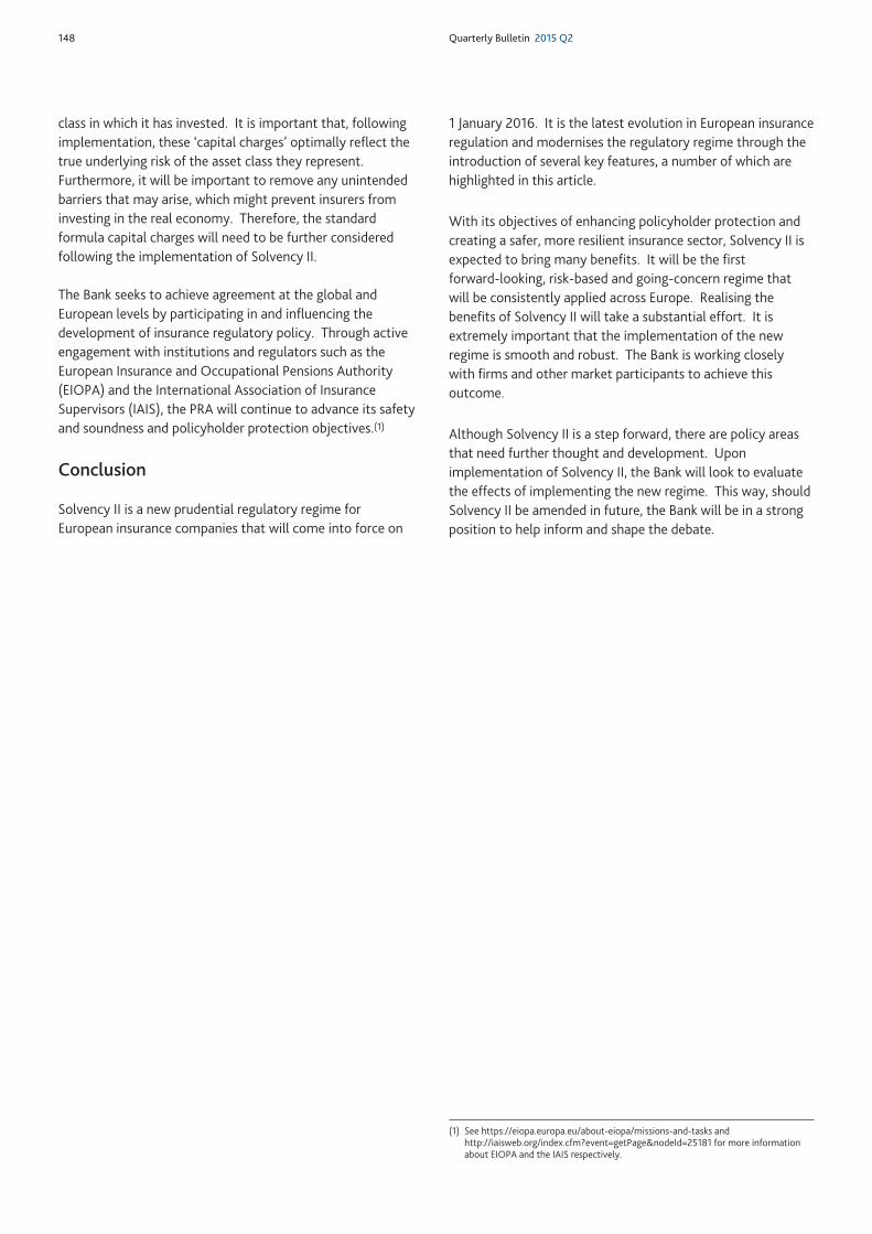
148 Quarterly Bulletin 2015 Q2
class in which it has invested. It is important that, followingimplementation, these ‘capital charges’ optimally reflect thetrue underlying risk of the asset class they represent.Furthermore, it will be important to remove any unintendedbarriers that may arise, which might prevent insurers frominvesting in the real economy. Therefore, the standardformula capital charges will need to be further consideredfollowing the implementation of Solvency II.
The Bank seeks to achieve agreement at the global andEuropean levels by participating in and influencing thedevelopment of insurance regulatory policy. Through activeengagement with institutions and regulators such as theEuropean Insurance and Occupational Pensions Authority(EIOPA) and the International Association of InsuranceSupervisors (IAIS), the PRA will continue to advance its safetyand soundness and policyholder protection objectives.(1)
Conclusion
Solvency II is a new prudential regulatory regime forEuropean insurance companies that will come into force on
1 January 2016. It is the latest evolution in European insuranceregulation and modernises the regulatory regime through theintroduction of several key features, a number of which arehighlighted in this article.
With its objectives of enhancing policyholder protection andcreating a safer, more resilient insurance sector, Solvency II isexpected to bring many benefits. It will be the firstforward-looking, risk-based and going-concern regime thatwill be consistently applied across Europe. Realising thebenefits of Solvency II will take a substantial effort. It isextremely important that the implementation of the newregime is smooth and robust. The Bank is working closelywith firms and other market participants to achieve thisoutcome.
Although Solvency II is a step forward, there are policy areasthat need further thought and development. Uponimplementation of Solvency II, the Bank will look to evaluatethe effects of implementing the new regime. This way, shouldSolvency II be amended in future, the Bank will be in a strongposition to help inform and shape the debate.
(1) See https://eiopa.europa.eu/about-eiopa/missions-and-tasks andhttp://iaisweb.org/index.cfm?event=getPage&nodeId=25181 for more informationabout EIOPA and the IAIS respectively.
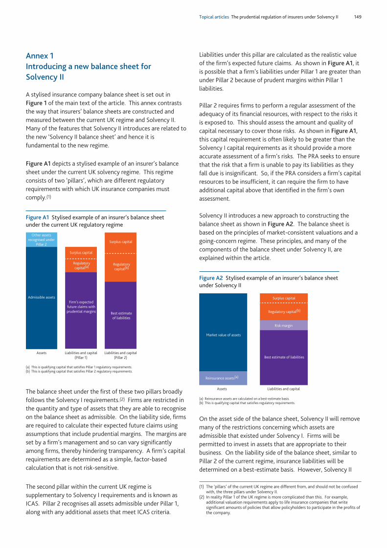
Topical articles The prudential regulation of insurers under Solvency II 149
Annex 1Introducing a new balance sheet forSolvency II
A stylised insurance company balance sheet is set out inFigure 1 of the main text of the article. This annex contraststhe way that insurers’ balance sheets are constructed andmeasured between the current UK regime and Solvency II.Many of the features that Solvency II introduces are related tothe new ‘Solvency II balance sheet’ and hence it isfundamental to the new regime.
Figure A1 depicts a stylised example of an insurer’s balancesheet under the current UK solvency regime. This regimeconsists of two ‘pillars’, which are different regulatoryrequirements with which UK insurance companies mustcomply.(1)
The balance sheet under the first of these two pillars broadlyfollows the Solvency I requirements.(2) Firms are restricted inthe quantity and type of assets that they are able to recogniseon the balance sheet as admissible. On the liability side, firmsare required to calculate their expected future claims usingassumptions that include prudential margins. The margins areset by a firm’s management and so can vary significantlyamong firms, thereby hindering transparency. A firm’s capitalrequirements are determined as a simple, factor-basedcalculation that is not risk-sensitive.
The second pillar within the current UK regime issupplementary to Solvency I requirements and is known asICAS. Pillar 2 recognises all assets admissible under Pillar 1,along with any additional assets that meet ICAS criteria.
Liabilities under this pillar are calculated as the realistic valueof the firm’s expected future claims. As shown in Figure A1, itis possible that a firm’s liabilities under Pillar 1 are greater thanunder Pillar 2 because of prudent margins within Pillar 1liabilities.
Pillar 2 requires firms to perform a regular assessment of theadequacy of its financial resources, with respect to the risks itis exposed to. This should assess the amount and quality ofcapital necessary to cover those risks. As shown in Figure A1,this capital requirement is often likely to be greater than theSolvency I capital requirements as it should provide a moreaccurate assessment of a firm’s risks. The PRA seeks to ensurethat the risk that a firm is unable to pay its liabilities as theyfall due is insignificant. So, if the PRA considers a firm’s capitalresources to be insufficient, it can require the firm to haveadditional capital above that identified in the firm’s ownassessment.
Solvency II introduces a new approach to constructing thebalance sheet as shown in Figure A2. The balance sheet isbased on the principles of market-consistent valuations and agoing-concern regime. These principles, and many of thecomponents of the balance sheet under Solvency II, areexplained within the article.
On the asset side of the balance sheet, Solvency II will removemany of the restrictions concerning which assets areadmissible that existed under Solvency I. Firms will bepermitted to invest in assets that are appropriate to theirbusiness. On the liability side of the balance sheet, similar toPillar 2 of the current regime, insurance liabilities will bedetermined on a best-estimate basis. However, Solvency II
Other assetsrecognised under
Pillar 2
Admissible assets
Surplus capital
Regulatorycapital(a)
Firm’s expectedfuture claims withprudential margins
Surplus capital
Regulatorycapital(b)
Best estimateof liabilities
Liabilities and capital(Pillar 1)
Liabilities and capital(Pillar 2)
Assets
(a) This is qualifying capital that satisfies Pillar 1 regulatory requirements.(b) This is qualifying capital that satisfies Pillar 2 regulatory requirements.
Figure A1 Stylised example of an insurer’s balance sheetunder the current UK regulatory regime
Market value of assets
Reinsurance assets(a)
Surplus capital
Risk margin
Best estimate of liabilities
Liabilities and capitalAssets
Regulatory capital(b)
(a) Reinsurance assets are calculated on a best-estimate basis.(b) This is qualifying capital that satisfies regulatory requirements.
Figure A2 Stylised example of an insurer’s balance sheetunder Solvency II
(1) The ‘pillars’ of the current UK regime are different from, and should not be confusedwith, the three pillars under Solvency II.
(2) In reality Pillar 1 of the UK regime is more complicated than this. For example,additional valuation requirements apply to life insurance companies that writesignificant amounts of policies that allow policyholders to participate in the profits ofthe company.

150 Quarterly Bulletin 2015 Q2
introduces a new component to the valuation of liabilities: a‘risk margin’. The risk margin is fundamental to Solvency IIbeing a market-consistent and a going-concern regime and isdiscussed in the box on page 144. Finally, Solvency IIintroduces forward-looking, risk-based capital requirements,which firms can calculate using a standard formula or internalmodel. In the example shown in Figure A2, the firm’s capitalis in excess of capital requirements.
Solvency II ushers in a single solvency assessment forEuropean insurers. The convergence in the preparation ofinsurers’ balance sheets across Europe will address thedisparate requirements that persisted under Solvency I. Thiswill lead to more consistent solvency reporting and a betterunderstanding of the risks faced by insurers.
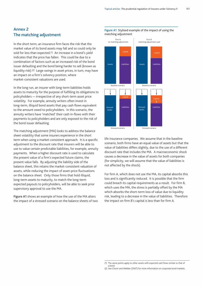
Topical articles The prudential regulation of insurers under Solvency II 151
Annex 2The matching adjustment
In the short term, an insurance firm faces the risk that themarket value of its bond assets may fall and so could only besold for less than expected.(1) An increase in a bond’s yieldindicates that the price has fallen. This could be due to acombination of factors such as an increased risk of the bondissuer defaulting and the bond being harder to sell (known asliquidity risk).(2) Large swings in asset prices, in turn, may havean impact on a firm’s solvency position, wheremarket-consistent valuations are used.
In the long run, an insurer with long-term liabilities holdsassets to maturity for the purpose of fulfilling its obligations topolicyholders — irrespective of any short-term asset pricevolatility. For example, annuity writers often invest inlong-term, illiquid bond assets that pay cash flows equivalentto the amount owed to policyholders. In this scenario, theannuity writers have ‘matched’ their cash in-flows with theirpayments to policyholders and are only exposed to the risk ofthe bond issuer defaulting.
The matching adjustment (MA) looks to address the balancesheet volatility that some insurers experience in the shortterm when using a market-consistent approach. It is a specificadjustment to the discount rate that insurers will be able touse to value certain predictable liabilities, for example, annuitypayments. When a higher discount rate is used to calculatethe present value of a firm’s expected future claims, thepresent value falls. By adjusting the liability side of thebalance sheet, this retains the market-consistent valuation ofassets, while reducing the impact of asset-price fluctuationson the balance sheet. Only those firms that hold illiquid,long-term assets to maturity, to match the long-termexpected payouts to policyholders, will be able to seek priorsupervisory approval to use the MA.
Figure A1 shows an example of how the use of the MA altersthe impact of a stressed scenario on the balance sheets of two
life insurance companies. We assume that in the baselinescenario, both firms have an equal value of assets but that thevalue of liabilities differs slightly, due to the use of a differentdiscount rate that includes the MA. A macroeconomic shockcauses a decrease in the value of assets for both companies(for simplicity, we will assume that the value of liabilities isnot affected by the shock).
For firm A, which does not use the MA, its capital absorbs thisloss and is significantly reduced. It is possible that the firmcould breach its capital requirements as a result. For firm B,which uses the MA, the stress is partially offset by the MAwhich absorbs the short-term loss of value due to liquidityrisk, leading to a decrease in the value of liabilities. Thereforethe impact on firm B’s capital is less than for firm A.
Firm A:no matching adjustment
Firm B:matching adjustment used
Baseline scenario
Stressed scenario
Baseline scenario
Stressed scenario
Assets
Capital
Liabilities
Capital
LiabilitiesAssets
Stressedassets
Stressedassets
CapitalCapital
Liabilities Liabilities
Figure A1 Stylised example of the impact of using thematching adjustment
(1) The same points apply to other assets with expected cash flows similar to that ofa bond.
(2) See Churm and Webber (2007) for more information on corporate bond markets.
152 Quarterly Bulletin 2015 Q2
References
Bank of England (2014a), ‘The PRA’s approach to insurance supervision’, available atwww.bankofengland.co.uk/publications/Documents/praapproach/insuranceappr1406.pdf.
Bank of England (2014b), ‘The Bank of England’s approach to resolution’, October, available atwww.bankofengland.co.uk/financialstability/Documents/resolution/apr231014.pdf.
Bank of England (2015a), ‘Solvency II: a new regime for insurers’, Prudential Regulation Authority Policy Statement PS2/15, March, available atwww.bankofengland.co.uk/pra/Documents/publications/ps/2015/ps215.pdf.
Bank of England (2015b), ‘Strengthening individual accountability in banking and insurance — responses to CP14/14 and CP26/14’, PrudentialRegulation Authority Policy Statement PS3/15, March, available at www.bankofengland.co.uk/pra/Documents/publications/ps/2015/ps315.pdf.
Breckenridge, J, Farquharson, J and Hendon, R (2014), ‘The role of business model analysis in the supervision of insurers’, Bank of EnglandQuarterly Bulletin, Vol. 54, No. 1, pages 49–57, available atwww.bankofengland.co.uk/publications/Documents/quarterlybulletin/2014/qb14q105.pdf.
Carney, M (2014), ‘Putting the right ideas into practice’, available atwww.bankofengland.co.uk/publications/Documents/speeches/2014/speech757.pdf.
Churm, R and Webber, L (2007), ‘Decomposing corporate bond spreads’, Bank of England Quarterly Bulletin, Vol. 47, No. 4, pages 533–41,available at www.bankofengland.co.uk/publications/Documents/quarterlybulletin/qb070403.pdf.
Commission Delegated Regulation (EU) 2015/35 (2014), ‘Supplementing Directive 2009/138/EC’, OJ L 12.
Conference of insurance supervisory services of the member states of the European Union — prepared under chairmanship of Dr HelmutMüller (1997), ‘Solvency of insurance undertakings’, available athttp://archive.eiopa.europa.eu/fileadmin/tx_dam/files/publications/reports/report_dt_9704.pdf.
Conference of insurance supervisory services of the member states of the European Union — prepared under chairmanship of Paul Sharma (2002), ‘Prudential supervision of insurance undertakings’, available atwww.ec.europa.eu/internal_market/insurance/docs/solvency/impactassess/annex-c02_en.pdf.
Debbage, S and Dickinson, S (2013), ‘The rationale for the prudential regulation and supervision of insurers’, Bank of EnglandQuarterly Bulletin, Vol. 53, No. 3, pages 216–22, available atwww.bankofengland.co.uk/publications/Documents/quarterlybulletin/2013/qb130303.pdf.
Directive 98/78/EC (1998), ‘The supplementary supervision of insurance undertakings in an insurance group’, OJ L 330/1.
Directive 2009/138/EC (2009), ‘The taking-up and pursuit of business of Insurance and Reinsurance’, OJ L 335.
Directive 2014/51/EU (2014), ‘Amending Directives 2003/71/EC and 2009/138/EC and Regulations (EC) No 1060/2009, (EU) No 1094/2010and (EU) No 1095/2010’, OJ L153/1.
Financial Services Authority (2005), ‘Insurance sector briefing: delivering the Tiner insurance reforms’, available atwww.fsa.gov.uk/pubs/other/tiner_insurance_report.pdf.
Gracie, A, Chennells, L and Menary, M (2014), ‘The Bank of England’s approach to resolving failed institutions’, Bank of EnglandQuarterly Bulletin, Vol. 54, No. 4, pages 409–18, available atwww.bankofengland.co.uk/publications/Documents/quarterlybulletin/2014/qb14q404.pdf.
HM Treasury (2015), ‘The Solvency II regulations 2015’, SI 2015/575.
International Association of Insurance Supervisors (2013), ‘Global systemically important insurers: policy measures’, available atwww.iaisweb.org/index.cfm?event=getPage&nodeId=25233.
Kempler, C, Flamée, M, Yang, C and Windels, P (2010), Global perspectives on insurance today, Palgrave Macmillan, Chapter 5.
KPMG (2002), ‘Study into the methodologies to assess the overall financial position of an insurance undertaking from the perspective ofprudential supervision’, available at www.ec.europa.eu/finance/insurance/docs/solvency/impactassess/annex-c01a_en.pdf.
Prudential Regulation Authority Rulebook, available at www.fshandbook.info/FS/prarulebook.jsp.
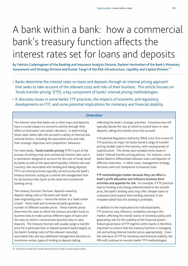
Topical articles A bank within a bank 153
• Banks determine the interest rates on loans and deposits through an internal pricing approachthat seeks to take account of the relevant costs and risks of their business. This article focuses on‘funds transfer pricing’ (FTP), a key component of banks’ internal pricing methodologies.
• It discusses issues in some banks’ FTP practices, the impacts of economic and regulatorydevelopments on FTP, and some potential implications for monetary and financial stability.
A bank within a bank: how a commercialbank’s treasury function affects theinterest rates set for loans and depositsBy Fabrizio Cadamagnani of the Banking and Insurance Analysis Division, Rashmi Harimohan of the Bank’s MonetaryAssessment and Strategy Division and Kumar Tangri of the Risk Infrastructure, Liquidity and Capital Division.(1)
(1) The authors would like to thank Steve Perry for his help in producing this article.
Overview
The interest rates that banks set on their loans and depositshave a crucial impact on economic activity through theireffect on borrowers’ and savers’ decisions. In determiningthese rates, banks take into account a variety of internal andexternal factors, including the associated costs and risks,their strategic objectives and competitors’ behaviour.
For most banks, ‘funds transfer pricing’ (FTP) is part of theprocess of setting retail and commercial interest rates and isa mechanism designed to account for the cost of funds facedby banks as well as the associated liquidity, interest rate andcurrency risks associated with lending and taking deposits.FTP is an internal process typically carried out by the bank’streasury function, acting as a central risk management hubfor all business lines (such as the retail and commercialbanking arms).
The treasury function ‘borrows’ deposits raised bydeposit-taking units of the bank and ‘lends’ toloan-originating units — hence the notion of a ‘bank withina bank’. Most retail and commercial banks generate anumber of different transfer prices. These transfer pricesdetermine the rates at which the treasury provides funds tobusiness lines to make various different types of loans andthe rates at which it remunerates business lines to raisedeposits. The treasury function will usually assign a transferprice for a particular loan or deposit product based largely onthe bank’s funding costs (of the relevant maturity),associated risks and any additional management decisions toincentivise certain types of lending or deposit-taking,
reflecting the bank’s strategic priorities. A business line willtypically decide the rate at which to extend loans or raisedeposits, taking the transfer price into account.
A Prudential Regulation Authority (PRA) cross-firm review ofFTP practices at major UK banks found a range of transferpricing models used in the industry, with varying levels ofsophistication. The review also revealed some issues inbanks’ internal transfer pricing policies. For instance, somebanks failed to differentiate between loans and deposits ofdifferent maturities. In other cases, management strategydecisions were not transparent to business lines.
FTP methodologies matter because they can affect abank’s profit allocation and influence business lines’activities and appetite for risk. For example, if FTP practiceslead to funding costs being underestimated in the transferprice, the bank’s lending units may offer cheaper loans tocustomers (and expand their lending volumes) in themistaken belief that this lending is profitable.
In addition to the implications for individual banks,FTP practices may influence competitor pricing in themarket, affecting the overall stance of monetary policy andgenerating risks for the stability of the financial system.Robust governance of FTP regimes within banks is thereforeimportant to ensure that the treasury function is managingrisk and setting internal transfer prices appropriately. Giventhe relevance of FTP for monetary and financial stability, thePRA will continue to monitor banks’ FTP methodologies.
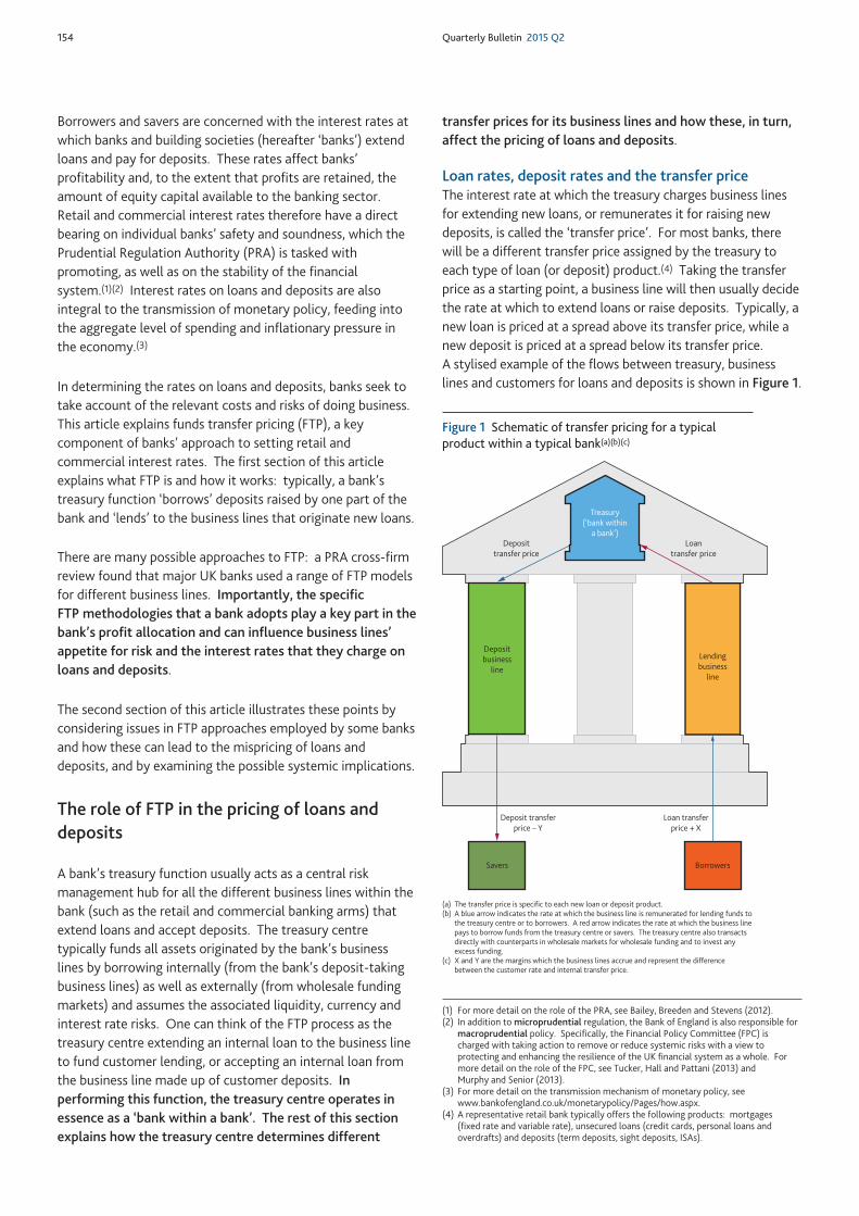
154 Quarterly Bulletin 2015 Q2
Borrowers and savers are concerned with the interest rates atwhich banks and building societies (hereafter ‘banks’) extendloans and pay for deposits. These rates affect banks’profitability and, to the extent that profits are retained, theamount of equity capital available to the banking sector.Retail and commercial interest rates therefore have a directbearing on individual banks’ safety and soundness, which thePrudential Regulation Authority (PRA) is tasked withpromoting, as well as on the stability of the financialsystem.(1)(2) Interest rates on loans and deposits are alsointegral to the transmission of monetary policy, feeding intothe aggregate level of spending and inflationary pressure inthe economy.(3)
In determining the rates on loans and deposits, banks seek totake account of the relevant costs and risks of doing business.This article explains funds transfer pricing (FTP), a keycomponent of banks’ approach to setting retail andcommercial interest rates. The first section of this articleexplains what FTP is and how it works: typically, a bank’streasury function ‘borrows’ deposits raised by one part of thebank and ‘lends’ to the business lines that originate new loans.
There are many possible approaches to FTP: a PRA cross-firmreview found that major UK banks used a range of FTP modelsfor different business lines. Importantly, the specificFTP methodologies that a bank adopts play a key part in thebank’s profit allocation and can influence business lines’appetite for risk and the interest rates that they charge onloans and deposits.
The second section of this article illustrates these points byconsidering issues in FTP approaches employed by some banksand how these can lead to the mispricing of loans anddeposits, and by examining the possible systemic implications.
The role of FTP in the pricing of loans anddeposits
A bank’s treasury function usually acts as a central riskmanagement hub for all the different business lines within thebank (such as the retail and commercial banking arms) thatextend loans and accept deposits. The treasury centretypically funds all assets originated by the bank’s businesslines by borrowing internally (from the bank’s deposit-takingbusiness lines) as well as externally (from wholesale fundingmarkets) and assumes the associated liquidity, currency andinterest rate risks. One can think of the FTP process as thetreasury centre extending an internal loan to the business lineto fund customer lending, or accepting an internal loan fromthe business line made up of customer deposits. Inperforming this function, the treasury centre operates inessence as a ‘bank within a bank’. The rest of this sectionexplains how the treasury centre determines different
transfer prices for its business lines and how these, in turn,affect the pricing of loans and deposits.
Loan rates, deposit rates and the transfer priceThe interest rate at which the treasury charges business linesfor extending new loans, or remunerates it for raising newdeposits, is called the ‘transfer price’. For most banks, therewill be a different transfer price assigned by the treasury toeach type of loan (or deposit) product.(4) Taking the transferprice as a starting point, a business line will then usually decidethe rate at which to extend loans or raise deposits. Typically, anew loan is priced at a spread above its transfer price, while anew deposit is priced at a spread below its transfer price.A stylised example of the flows between treasury, businesslines and customers for loans and deposits is shown in Figure 1.
Treasury(‘bank within
a bank’)
Depositbusiness
line
Lendingbusiness
line
BorrowersSavers
Deposittransfer price
Deposit transferprice – Y
Loantransfer price
Loan transferprice + X
Figure 1 Schematic of transfer pricing for a typicalproduct within a typical bank(a)(b)(c)
(a) The transfer price is specific to each new loan or deposit product.(b) A blue arrow indicates the rate at which the business line is remunerated for lending funds to
the treasury centre or to borrowers. A red arrow indicates the rate at which the business linepays to borrow funds from the treasury centre or savers. The treasury centre also transactsdirectly with counterparts in wholesale markets for wholesale funding and to invest anyexcess funding.
(c) X and Y are the margins which the business lines accrue and represent the differencebetween the customer rate and internal transfer price.
(1) For more detail on the role of the PRA, see Bailey, Breeden and Stevens (2012).(2) In addition to microprudential regulation, the Bank of England is also responsible for
macroprudential policy. Specifically, the Financial Policy Committee (FPC) ischarged with taking action to remove or reduce systemic risks with a view toprotecting and enhancing the resilience of the UK financial system as a whole. Formore detail on the role of the FPC, see Tucker, Hall and Pattani (2013) andMurphy and Senior (2013).
(3) For more detail on the transmission mechanism of monetary policy, seewww.bankofengland.co.uk/monetarypolicy/Pages/how.aspx.
(4) A representative retail bank typically offers the following products: mortgages(fixed rate and variable rate), unsecured loans (credit cards, personal loans andoverdrafts) and deposits (term deposits, sight deposits, ISAs).

Topical articles A bank within a bank 155
The spread above or below the transfer price reflects internaland external factors, such as other costs that the business linefaces, associated with lending and deposit activities; the rateof return that business lines would like to generate on theirloans and deposits, the bank’s strategic objectives andcompetitor behaviour.
Pricing loans versus depositsFor lending rates, the spread above the transfer price willinclude the costs associated with any expected loss on theloan, the capital charge associated with the loan and otherfactors such as the bank’s operating costs and margins (ormark-up). The expected loss represents the averageexpectation of loss associated with a loan and can be thoughtof as a combination of the likelihood that a borrower willdefault and the loss suffered by a bank if the default were tooccur. Estimates for expected losses are affected by theoutlook for the creditworthiness of borrowers and generaleconomic conditions. The capital charge represents the costof capital to cover losses that exceed banks’ centralexpectations. The amount of capital needed to coverunexpected losses will be affected by national andinternational regulation, including the Basel III minimumcapital requirements. Operating costs include the bank’s costsassociated with the origination and servicing of the loan suchas staff costs and other overheads. The margin, or mark-up,typically represents the amount lenders charge over theirmarginal costs to ensure that each loan extended generates anexpected rate of return.(1)
This is best understood by considering a stylised example forloan rates. In Figure 2, a bank’s business line pays a 2%transfer price to the treasury function but charges thecustomer 3.5% for a loan. The business line bears additionalcosts and risks associated with the loan of 1% in the form ofthe expected loss, capital charge and other operating costswhich are managed by the business line rather than centrallyby the treasury function. In this simple example, the businessline thus generates a 0.5% rate of return, or mark-up, on eachnew loan, that is the difference between the customer
rate (3.5%) and the transfer price (2%) and additionalcosts (1%).
The internal pricing of a deposit differs from that of a loansince a deposit is a source of funds for a bank. Unlike loans,where the customer-facing business line pays the treasurycentre an internal price to originate the loan, the business linereceives an internal rebate for acquiring deposit funding. Thisrebate reflects the value to the bank of deposits gathered. Inthe stylised example in Figure 2, a bank’s business line receivesa 2% transfer price from the treasury centre but pays thecustomer only 1% on the deposit. This spread reflects thecosts associated with raising deposits as well as the rate ofreturn the business line aims to generate on each new deposit.
Components of the transfer priceEach transfer price is determined by the way in which thetreasury centre manages the risk of business lines’transactions. Typically the treasury centre does so bymatching the maturity and interest rate profile of new lendingand funding, together with the currencies in which they aretransacted, to manage liquidity, interest rate and currencyrisks centrally within the bank.
For a given currency, the FTP process usually involves assigningto each loan or deposit product a curve that reflects itstransfer price at different maturities. The FTP curve usuallyreflects the bank’s cost of funding and any strategy decisions(known as ‘management overlays’) that the treasury centremay wish to apply to incentivise desired behaviour within thebusiness lines. The transfer price for a loan (or deposit) is thepoint on the FTP curve that reflects the loan’s maturity, withthe addition of the cost of holding a buffer of liquid assets.The rest of this section explains these different components ofa bank’s FTP curve in more detail.
While the marginal funding cost curve is usually applieduniversally to all products and business lines of the bank,the application of management overlays means that theFTP curve will typically be specific to each loan or depositproduct.
The marginal funding costBanks finance their lending activities with various sources offunding.(2) When a bank extends a new loan, it will considerthe cost of raising additional funding to finance the loan. Themarginal funding cost associated with the loan is thus a keydriver of the transfer price.
Typically in the transfer price for a new loan, the funding costis calculated on a maturity-matched basis to reflect liquidityrisk. The treasury centre also typically manages interest rate
(1) For more details, see Button, Pezzini and Rossiter (2010).(2) For more details, see Beau et al (2014).
Stylised example — loan
FTP
0.5%
0.5%
0.4%
0.1%
2.0%
Other costs
Mark-up
Capital charge
Expected loss
3.5% customer rate
Stylised example — deposit
FTP 2.0%
0.6% Other costs
0.4% Mark-down
1% customer rate
Figure 2 Stylised examples of loan and deposit pricing
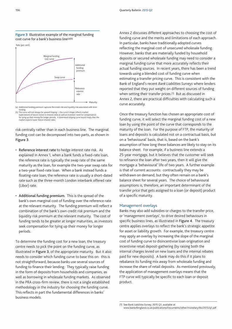
156 Quarterly Bulletin 2015 Q2
risk centrally rather than in each business line. The marginalfunding cost can be decomposed into two parts, as shown inFigure 3.
• Reference interest rate to hedge interest rate risk. Asexplained in Annex 1, when a bank funds a fixed-rate loan,the reference rate is typically the swap rate of the samematurity as the loan, for example the two-year swap rate fora two-year fixed-rate loan. When a bank instead funds afloating-rate loan, the reference rate is usually a short-datedrate such as the three-month London interbank offered rate(Libor) rate.
• Additional funding premium. This is the spread of thebank’s own marginal cost of funding over the reference rateat the relevant maturity. The funding premium will reflect acombination of the bank’s own credit risk premium and theliquidity risk premium at the relevant maturity. The cost offunding tends to be greater at longer maturities, as investorsseek compensation for tying up their money for longerperiods.
To determine the funding cost for a new loan, the treasurycentre needs to pick the point on the funding curve, asillustrated in Figure 3, of the appropriate maturity. But it alsoneeds to consider which funding curve to base this on: this isnot straightforward, because banks use several sources offunding to finance their lending. They typically raise fundingin the form of deposits from households and companies, aswell as borrowing in wholesale funding markets. As observedin the PRA cross-firm review, there is not a single establishedmethodology in the industry for choosing the funding curve.This reflects in part the fundamental differences in banks’business models.
Annex 2 discusses different approaches to choosing the cost offunding curve and the merits and limitations of each approach.In particular, banks have traditionally adopted curvesreflecting the marginal cost of unsecured wholesale funding.However, banks that are materially funded by householddeposits or secured wholesale funding may need to consider amarginal funding curve that more accurately reflects theiractual funding sources. In recent years, there has been a trendtowards using a blended cost of funding curve whenestimating a transfer pricing curve. This is consistent with theBank of England’s recent Bank Liabilities Surveys where lendersreported that they put weight on different sources of fundingwhen setting their transfer prices.(1) But as discussed inAnnex 2, there are practical difficulties with calculating such acurve accurately.
Once the treasury function has chosen an appropriate cost offunding curve, it will select the marginal funding cost of a newloan by using the point of the curve that corresponds to thematurity of the loan. For the purpose of FTP, the maturity ofloans and deposits is calculated not on a contractual basis, buton a ‘behavioural’ basis, that is, based on the bank’sassumption of how long these balances are likely to stay on itsbalance sheet. For example, if a business line extends a25-year mortgage, but it believes that the customer will seekto refinance the loan after two years, then it will give themortgage a ‘behavioural’ life of two years. A further exampleis that of current accounts: contractually they may bewithdrawn on demand, but they often remain on a bank’sbalance sheet for several years. The choice of behaviouralassumptions is, therefore, an important determinant of thetransfer price that gets assigned to a loan (or deposit) productof a specific maturity.
Management overlaysBanks may also add subsidies or charges to the transfer price,or ‘management overlays’, to drive desired behaviours inspecific business lines, as illustrated in Figure 4. The treasurycentre applies overlays to reflect the bank’s strategic appetitefor asset or liability growth. For example, the treasury centremay apply an overlay by increasing the slope of the marginalcost of funding curve to disincentivise loan origination andincentivise retail deposit-gathering (by raising both theinternal charges levied on new loans and the internal rebatespaid for new deposits). A bank may do this if it plans torebalance its funding mix away from wholesale funding andincrease the share of retail deposits. As mentioned previously,the application of management overlays means that theFTP curve will typically be specific to each loan or depositproduct.
Maturity
Rate (per cent)
Swap curve
Reference interest rate
Marginal funding cost curve
Additional funding premium
(a) Additional funding premium captures the credit risk and liquidity risk associated with termfunding.
(b) The curve will not always be upward sloping — the curve’s shape reflects marketexpectations of future moves in interest rates as well as investors’ need for compensationfor tying up their money for longer periods. A downward-sloping curve would imply that themarket expects lower future interest rates.
Figure 3 Illustrative example of the marginal fundingcost curve for a bank’s business line(a)(b)
(1) See Bank Liabilities Survey, 2015 Q1, available atwww.bankofengland.co.uk/publications/Documents/other/monetary/bls/2015/q1.pdf.
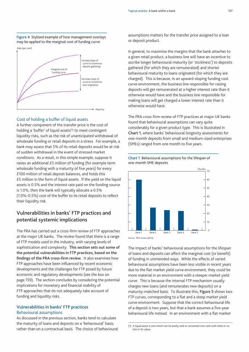
Topical articles A bank within a bank 157
Cost of holding a buffer of liquid assetsA further component of the transfer price is the cost ofholding a ‘buffer’ of liquid assets(1) to meet contingentliquidity risks, such as the risk of unanticipated withdrawal ofwholesale funding or retail deposits in a stress. For example, abank may assess that 5% of its retail deposits would be at riskof sudden withdrawal in the event of stressed marketconditions. As a result, in this simple example, suppose itraises an additional £5 million of funding (for example termwholesale funding with a maturity of five years) for every£100 million of retail deposit balances, and holds this£5 million in the form of liquid assets. If the yield on the liquidassets is 0.5% and the interest rate paid on the funding sourceis 1.0%, then the bank will typically allocate a 0.5%(1.0%–0.5%) cost of the buffer to its retail deposits to reflecttheir liquidity risk.
Vulnerabilities in banks’ FTP practices andpotential systemic implications
The PRA has carried out a cross-firm review of FTP approachesat the major UK banks. The review found that there is a rangeof FTP models used in the industry, with varying levels ofsophistication and complexity. This section sets out some ofthe potential vulnerabilities in FTP practices, based on thefindings of the PRA cross-firm review. It also examines howFTP approaches have been influenced by recent economicdevelopments and the challenges for FTP posed by futureeconomic and regulatory developments (see the box onpage 159). The section concludes by considering the potentialimplications for monetary and financial stability ofFTP approaches that do not adequately take account offunding and liquidity risks.
Vulnerabilities in banks’ FTP practicesBehavioural assumptionsAs discussed in the previous section, banks tend to calculatethe maturity of loans and deposits on a ‘behavioural’ basis,rather than on a contractual basis. The choice of behavioural
assumptions matters for the transfer price assigned to a loanor deposit product.
In general, to maximise the margins that the bank attaches toa given retail product, a business line will have an incentive toascribe longer behavioural maturity (or ‘stickiness’) to depositsgathered (for which they are remunerated) and shorterbehavioural maturity to loans originated (for which they arecharged). This is because, in an upward-sloping funding costcurve environment, the business line responsible for raisingdeposits will get remunerated at a higher interest rate than itotherwise would have and the business line responsible formaking loans will get charged a lower interest rate than itotherwise would have.
The PRA cross-firm review of FTP practices at major UK banksfound that behavioural assumptions can vary quiteconsiderably for a given product type. This is illustrated inChart 1, where banks’ behavioural longevity assessments forone-month deposits from small and medium-sized enterprises(SMEs) ranged from one month to five years.
The impact of banks’ behavioural assumptions for the lifespanof loans and deposits can affect the marginal cost (or benefit)of funding in unintended ways. While the effects of variedbehavioural assumptions have been less visible in recent yearsdue to the flat market yield curve environment, they could bemore material in an environment with a steeper market yieldcurve. This is because the internal FTP mechanism usuallycharges new loans (and remunerates new deposits) on amaturity-matched basis. To illustrate this, Figure 5 shows twoFTP curves, corresponding to a flat and a steep market yieldcurve environment. Suppose that the correct behavioural lifeof a deposit is two years, but that a bank assumes a five-yearbehavioural life instead. In an environment with a flat market
Increase slope of curve to incentivise deposit-gathering
Decrease slope of curve to incentivise loan origination
Marginal cost of funding curve
Maturity
Rate (per cent)
Figure 4 Stylised example of how management overlaysmay be applied to the marginal cost of funding curve
Bank 1 Bank 2 Bank 3 Bank 4 Bank 5
Months
0
10
20
30
40
50
60
70
Source: PRA review (2013).
Chart 1 Behavioural assumptions for the lifespan ofone-month SME deposits
(1) A liquid asset is one which can be easily sold or converted into cash with little or noloss in its value.
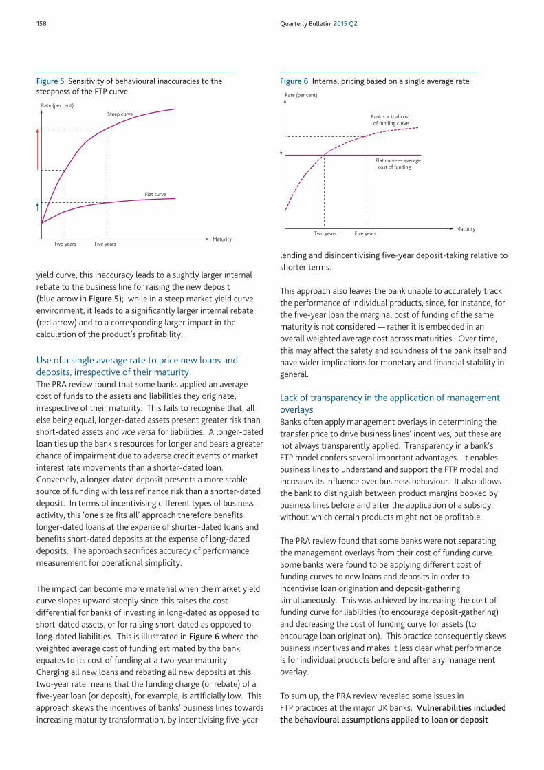
158 Quarterly Bulletin 2015 Q2
yield curve, this inaccuracy leads to a slightly larger internalrebate to the business line for raising the new deposit(blue arrow in Figure 5); while in a steep market yield curveenvironment, it leads to a significantly larger internal rebate(red arrow) and to a corresponding larger impact in thecalculation of the product’s profitability.
Use of a single average rate to price new loans anddeposits, irrespective of their maturityThe PRA review found that some banks applied an averagecost of funds to the assets and liabilities they originate,irrespective of their maturity. This fails to recognise that, allelse being equal, longer-dated assets present greater risk thanshort-dated assets and vice versa for liabilities. A longer-datedloan ties up the bank’s resources for longer and bears a greaterchance of impairment due to adverse credit events or marketinterest rate movements than a shorter-dated loan.Conversely, a longer-dated deposit presents a more stablesource of funding with less refinance risk than a shorter-dateddeposit. In terms of incentivising different types of businessactivity, this ‘one size fits all’ approach therefore benefitslonger-dated loans at the expense of shorter-dated loans andbenefits short-dated deposits at the expense of long-dateddeposits. The approach sacrifices accuracy of performancemeasurement for operational simplicity.
The impact can become more material when the market yieldcurve slopes upward steeply since this raises the costdifferential for banks of investing in long-dated as opposed toshort-dated assets, or for raising short-dated as opposed tolong-dated liabilities. This is illustrated in Figure 6 where theweighted average cost of funding estimated by the bankequates to its cost of funding at a two-year maturity.Charging all new loans and rebating all new deposits at thistwo-year rate means that the funding charge (or rebate) of afive-year loan (or deposit), for example, is artificially low. Thisapproach skews the incentives of banks’ business lines towardsincreasing maturity transformation, by incentivising five-year
lending and disincentivising five-year deposit-taking relative toshorter terms.
This approach also leaves the bank unable to accurately trackthe performance of individual products, since, for instance, forthe five-year loan the marginal cost of funding of the samematurity is not considered — rather it is embedded in anoverall weighted average cost across maturities. Over time,this may affect the safety and soundness of the bank itself andhave wider implications for monetary and financial stability ingeneral.
Lack of transparency in the application of managementoverlaysBanks often apply management overlays in determining thetransfer price to drive business lines’ incentives, but these arenot always transparently applied. Transparency in a bank’sFTP model confers several important advantages. It enablesbusiness lines to understand and support the FTP model andincreases its influence over business behaviour. It also allowsthe bank to distinguish between product margins booked bybusiness lines before and after the application of a subsidy,without which certain products might not be profitable.
The PRA review found that some banks were not separatingthe management overlays from their cost of funding curve.Some banks were found to be applying different cost offunding curves to new loans and deposits in order toincentivise loan origination and deposit-gatheringsimultaneously. This was achieved by increasing the cost offunding curve for liabilities (to encourage deposit-gathering)and decreasing the cost of funding curve for assets (toencourage loan origination). This practice consequently skewsbusiness incentives and makes it less clear what performanceis for individual products before and after any managementoverlay.
To sum up, the PRA review revealed some issues inFTP practices at the major UK banks. Vulnerabilities includedthe behavioural assumptions applied to loan or deposit
Five yearsTwo years
Steep curve
Flat curve
Maturity
Rate (per cent)
Figure 5 Sensitivity of behavioural inaccuracies to thesteepness of the FTP curve
Bank’s actual cost of funding curve
Flat curve — average cost of funding
Five yearsTwo yearsMaturity
Rate (per cent)
Figure 6 Internal pricing based on a single average rate
Topical articles A bank within a bank 159
Impact of economic and regulatorydevelopments on FTP
The recent financial crisis has had a major impact on banks’business models and their internal pricing methodologies. Thisbox examines how FTP practices have been affected byeconomic developments after the crisis, and how FTP practicesare likely to be affected by future economic and regulatorydevelopments.
Impact of post-crisis economic developmentsChanges in FTP methodologiesPrior to the crisis, some banks deemed funding to be readilyavailable and consequently did not adequately reflectliquidity and credit risk when pricing new loans and deposits.During the crisis, funding markets became less liquid, so bankshave started to include both an additional funding premiumand the cost of holding a liquid asset buffer in theirFTP methodologies. They have also had to consider a greaterrange of different funding curves when estimating theirtransfer price curve. This reflects a diversification in banks’sources of funding following the crisis.
Net interest marginThe economic environment after the crisis has also presentedchallenges for banks’ net interest margins — the differencebetween the interest charged on loans and paid on deposits.In response to the downturn, central banks widely reducedpolicy rates significantly; in the United Kingdom, Bank Rate fellsharply to a historical low of 0.5%. Prior to the crisis, bankstypically offered rates on new household deposits belowBank Rate. But the low-rate environment effectively placed alower bound (or ‘floor’) on the rates that banks offer on sightdeposits, since, if deposit rates were to become negative,depositors might withdraw their deposits and hold them ascash. As a result, the difference between Bank Rate and rateson sight deposits fell sharply and has been a source ofdownward pressure on banks’ net interest margins since thestart of the financial crisis. This pressure on banks’ net interestmargins may have led banks to make offsetting adjustments tomargins on other products, for example by raising the ratescharged on new loans or reducing rates on other (non-sightdeposit) savings products. However, if banks’ FTP models donot reflect the new environment, then individual business linesmay continue trading without adjusting rates, to the detrimentof the overall net interest margin. Appropriate governancearrangements are required to guard against this latter risk, sothat true product economics underpin business decisions.
Challenges from future regulatory and economicdevelopmentsRing-fencingIn the United Kingdom, the Independent Commission onBanking has set out proposals intended to insulate high street
banking businesses from riskier investment banking arms.Banks will have to put their UK retail banking business in aseparately capitalised subsidiary.(1) Similar reforms have beenpromoted in the European Union(2) and the United States.(3)
Among the key questions for banks is what the marginal costof funding should be for entities within and outside thisring-fence. Outside the ring fence, the marginal cost offunding curve might be based on wholesale secured andunsecured funding, whereas ring-fenced entities may need toconsider mainly retail and corporate deposits for theirmarginal funding. This could have implications for the waybanks estimate their marginal funding cost curves, particularlyfor banks that currently use a curve based on a single source offunding (see Annex 2).
Recovery and resolutionBanks are now required to have a plan in place that sets outhow they would wind-down in an orderly manner in the eventof resolution, reducing the impact on financial stability andrisks to the taxpayer.(4) One resulting issue is the possibleimpact on banks’ cost of capital and on ‘bail-inable’(5)
wholesale debt. The likely impact on debt funding costs willneed to be incorporated into banks’ transfer pricingmethodologies to ensure they are properly accounting for allcosts associated with their lending and deposit-takingactivities.
Impact of higher interest ratesAs the economy normalises, Bank Rate is likely to start torise.(6) The level of Bank Rate, and the shape of the marketyield curve, are likely to have implications for banks’profitability and how they manage their margins through FTP.
Among the key questions are the likely behaviour and pricingof sight deposits and current account balances, as depositorsare more incentivised to put their money to work in ahigher-rate environment. Migration of deposit balances awayfrom patterns established over the past five years may impactthe revenues which banks derive from them. FTP models mayneed to account for this potential change in the behaviour ofcustomer deposits.
(1) www.bankofengland.co.uk/publications/Pages/news/2014/125.aspx.(2) http://ec.europa.eu/finance/bank/structural-reform/index_en.htm.(3) www.federalreserve.gov/bankinforeg/volcker-rule/.(4) See PRA Policy Statement PS1/15, ‘Implementing the Bank Recovery and Resolution
Directive — response to CP13/14’, January 2015;www.bankofengland.co.uk/pra/Documents/publications/ps/2015/ps115.pdf.
(5) www.ecb.europa.eu/press/key/date/2013/html/sp130930.en.html.(6) But, as noted in the November 2014 Inflation Report, when Bank Rate does begin to
rise, the pace of rate increases is likely to be gradual, with Bank Rate probablyremaining below its historical average level for some time. Seewww.bankofengland.co.uk/publications/Documents/inflationreport/2014/ir14nov.pdf.
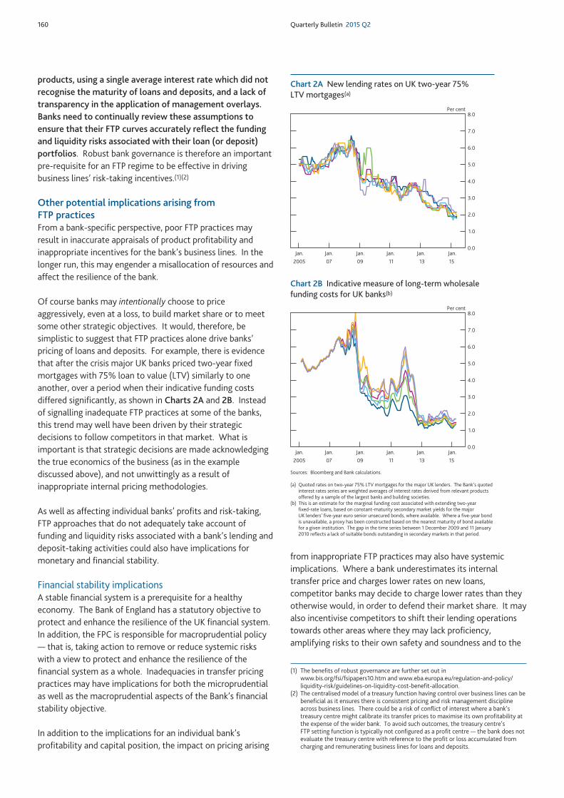
160 Quarterly Bulletin 2015 Q2
products, using a single average interest rate which did notrecognise the maturity of loans and deposits, and a lack oftransparency in the application of management overlays.Banks need to continually review these assumptions toensure that their FTP curves accurately reflect the fundingand liquidity risks associated with their loan (or deposit)portfolios. Robust bank governance is therefore an importantpre-requisite for an FTP regime to be effective in drivingbusiness lines’ risk-taking incentives.(1)(2)
Other potential implications arising fromFTP practicesFrom a bank-specific perspective, poor FTP practices mayresult in inaccurate appraisals of product profitability andinappropriate incentives for the bank’s business lines. In thelonger run, this may engender a misallocation of resources andaffect the resilience of the bank.
Of course banks may intentionally choose to priceaggressively, even at a loss, to build market share or to meetsome other strategic objectives. It would, therefore, besimplistic to suggest that FTP practices alone drive banks’pricing of loans and deposits. For example, there is evidencethat after the crisis major UK banks priced two-year fixedmortgages with 75% loan to value (LTV) similarly to oneanother, over a period when their indicative funding costsdiffered significantly, as shown in Charts 2A and 2B. Insteadof signalling inadequate FTP practices at some of the banks,this trend may well have been driven by their strategicdecisions to follow competitors in that market. What isimportant is that strategic decisions are made acknowledgingthe true economics of the business (as in the examplediscussed above), and not unwittingly as a result ofinappropriate internal pricing methodologies.
As well as affecting individual banks’ profits and risk-taking,FTP approaches that do not adequately take account offunding and liquidity risks associated with a bank’s lending anddeposit-taking activities could also have implications formonetary and financial stability.
Financial stability implicationsA stable financial system is a prerequisite for a healthyeconomy. The Bank of England has a statutory objective toprotect and enhance the resilience of the UK financial system.In addition, the FPC is responsible for macroprudential policy— that is, taking action to remove or reduce systemic riskswith a view to protect and enhance the resilience of thefinancial system as a whole. Inadequacies in transfer pricingpractices may have implications for both the microprudentialas well as the macroprudential aspects of the Bank’s financialstability objective.
In addition to the implications for an individual bank’sprofitability and capital position, the impact on pricing arising
from inappropriate FTP practices may also have systemicimplications. Where a bank underestimates its internaltransfer price and charges lower rates on new loans,competitor banks may decide to charge lower rates than theyotherwise would, in order to defend their market share. It mayalso incentivise competitors to shift their lending operationstowards other areas where they may lack proficiency,amplifying risks to their own safety and soundness and to the
(1) The benefits of robust governance are further set out inwww.bis.org/fsi/fsipapers10.htm and www.eba.europa.eu/regulation-and-policy/liquidity-risk/guidelines-on-liquidity-cost-benefit-allocation.
(2) The centralised model of a treasury function having control over business lines can bebeneficial as it ensures there is consistent pricing and risk management disciplineacross business lines. There could be a risk of conflict of interest where a bank’streasury centre might calibrate its transfer prices to maximise its own profitability atthe expense of the wider bank. To avoid such outcomes, the treasury centre’sFTP setting function is typically not configured as a profit centre — the bank does notevaluate the treasury centre with reference to the profit or loss accumulated fromcharging and remunerating business lines for loans and deposits.
0.0
1.0
2.0
3.0
4.0
5.0
6.0
7.0
8.0
Jan. Jan. Jan. Jan. Jan. Jan.
Per cent
2005 07 09 11 13 15
Chart 2A New lending rates on UK two-year 75%LTV mortgages(a)
0.0
1.0
2.0
3.0
4.0
5.0
6.0
7.0
8.0
Jan. Jan. Jan. Jan. Jan. Jan.
Per cent
2005 07 09 11 13 15
Sources: Bloomberg and Bank calculations.
(a) Quoted rates on two-year 75% LTV mortgages for the major UK lenders. The Bank’s quotedinterest rates series are weighted averages of interest rates derived from relevant productsoffered by a sample of the largest banks and building societies.
(b) This is an estimate for the marginal funding cost associated with extending two-yearfixed-rate loans, based on constant-maturity secondary market yields for the majorUK lenders’ five-year euro senior unsecured bonds, where available. Where a five-year bondis unavailable, a proxy has been constructed based on the nearest maturity of bond availablefor a given institution. The gap in the time series between 1 December 2009 and 11 January2010 reflects a lack of suitable bonds outstanding in secondary markets in that period.
Chart 2B Indicative measure of long-term wholesalefunding costs for UK banks(b)
Topical articles A bank within a bank 161
system as a whole. These behaviours could result in amisallocation of resources in the economy with an oversupplyof lending in certain markets. They could also haveimplications for the overall profitability and solvency of thebanking system.
Monetary policy implicationsThe Bank of England’s Monetary Policy Committee (MPC) hasa primary objective of delivering price stability, defined by theGovernment’s 2% CPI inflation target. The main instrumentof monetary policy is Bank Rate, the policy rate set by theMPC each month.(1) Bank Rate affects short-term marketinterest rates, which in turn influence a range of interest ratesset by commercial banks as well as asset prices and theexchange rate. These factors influence consumer and businessdemand and the aggregate level of spending and inflationarypressure in the economy.
Effective transmission of monetary policy depends on theextent to which changes in Bank Rate are passed through tomarket interest rates and the rates that banks charge on loansand pay on deposits. The extent of pass-through of Bank Rateto retail interest rates is largely determined by a range offactors such as banks’ overall funding costs, their strategicobjectives and their competitors’ behaviour. But it will alsodepend on whether the treasury functions in individual banksadequately pass on changes in Bank Rate, via internal transferpricing, to the different business lines.
As a result, bank FTP approaches can have implications for theoverall stance of monetary policy, by influencing the level ofspending and inflationary pressure in the economy. Where abank overestimates its internal transfer price and chargeshigher rates on new loans, its lending becomes less affordablefor households and companies. This can, in turn, lead to areduction in lending volumes in the economy. And if internaltransfer prices are underestimated, business lines might offercheaper, more affordable loans and originate more loans thanthey otherwise would have done. These effects would beexacerbated if competitor banks matched the pricing changes.And the more widespread these pricing changes, the greaterthe potential impact on the aggregate level of spending in theeconomy.
Conclusion
The rates that banks set on their loans and deposits have acrucial impact on economic activity through their effect onborrowers and savers’ decisions. Banks use FTP to helpdetermine these rates.
A PRA cross-firm review found that there are a range oftransfer pricing models used in the industry with varying levelsof sophistication, in part due to the range of banks’ businessmodels. The cross-firm review also revealed some potentialshortcomings of some banks’ FTP policies.
Internal FTP methodologies play a key part in profit allocationwithin a bank and influence business lines’ activities. Iffunding costs are underestimated, business lines may offercustomers cheaper loans and increase lending volumes in themistaken belief that they are profitable. If funding costs areoverestimated, business lines may mistakenly require highercustomer rates to remain profitable, making loans lesscompetitive and affordable and limiting volumes. In additionto the implications for individual banks, poor FTP practicesmay influence competitor pricing in the market, affecting thestance of overall monetary policy and generating risks for thestability of the financial system.
Of course banks may intentionally choose to priceaggressively, even at a loss, to build market share or to meetother strategic objectives. But it is important that suchdecisions are made acknowledging the true economics of thebusiness and that they are not made unwittingly as a result ofinappropriate internal pricing methodologies.
Robust governance of FTP regimes within banks is thereforeimportant to ensure that the treasury function is managingrisk and setting the internal transfer prices appropriately.Given the relevance of FTP for the Bank’s objectives, the PRAwill continue to monitor banks’ FTP methodologies, both on abank-specific and industry-wide basis.
(1) In March 2009 the MPC announced that in addition to setting Bank Rate, it wouldstart to inject money directly into the economy by purchasing financial assets —often known as quantitative easing. For more detail, please seewww.bankofengland.co.uk/monetarypolicy/Pages/qe/default.aspx.
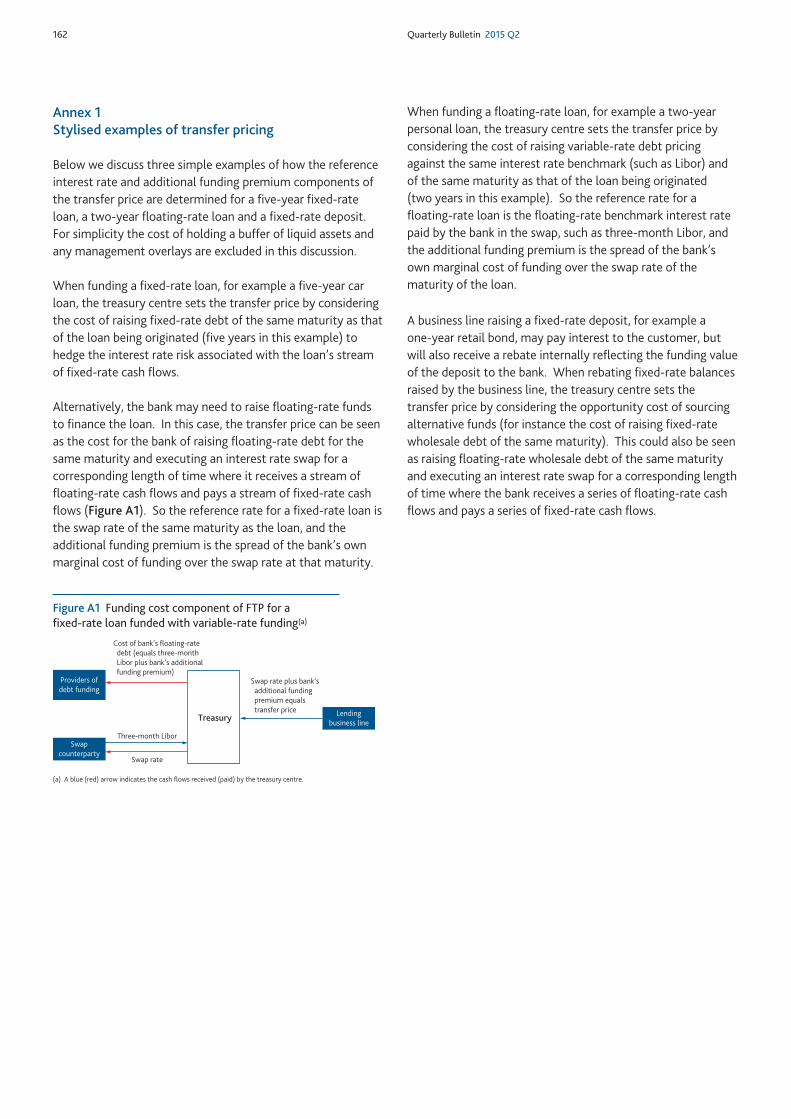
162 Quarterly Bulletin 2015 Q2
Annex 1Stylised examples of transfer pricing
Below we discuss three simple examples of how the referenceinterest rate and additional funding premium components ofthe transfer price are determined for a five-year fixed-rateloan, a two-year floating-rate loan and a fixed-rate deposit.For simplicity the cost of holding a buffer of liquid assets andany management overlays are excluded in this discussion.
When funding a fixed-rate loan, for example a five-year carloan, the treasury centre sets the transfer price by consideringthe cost of raising fixed-rate debt of the same maturity as thatof the loan being originated (five years in this example) tohedge the interest rate risk associated with the loan’s streamof fixed-rate cash flows.
Alternatively, the bank may need to raise floating-rate fundsto finance the loan. In this case, the transfer price can be seenas the cost for the bank of raising floating-rate debt for thesame maturity and executing an interest rate swap for acorresponding length of time where it receives a stream offloating-rate cash flows and pays a stream of fixed-rate cashflows (Figure A1). So the reference rate for a fixed-rate loan isthe swap rate of the same maturity as the loan, and theadditional funding premium is the spread of the bank’s ownmarginal cost of funding over the swap rate at that maturity.
When funding a floating-rate loan, for example a two-yearpersonal loan, the treasury centre sets the transfer price byconsidering the cost of raising variable-rate debt pricingagainst the same interest rate benchmark (such as Libor) andof the same maturity as that of the loan being originated(two years in this example). So the reference rate for afloating-rate loan is the floating-rate benchmark interest ratepaid by the bank in the swap, such as three-month Libor, andthe additional funding premium is the spread of the bank’sown marginal cost of funding over the swap rate of thematurity of the loan.
A business line raising a fixed-rate deposit, for example aone-year retail bond, may pay interest to the customer, butwill also receive a rebate internally reflecting the funding valueof the deposit to the bank. When rebating fixed-rate balancesraised by the business line, the treasury centre sets thetransfer price by considering the opportunity cost of sourcingalternative funds (for instance the cost of raising fixed-ratewholesale debt of the same maturity). This could also be seenas raising floating-rate wholesale debt of the same maturityand executing an interest rate swap for a corresponding lengthof time where the bank receives a series of floating-rate cashflows and pays a series of fixed-rate cash flows.
Cost of bank’s floating-rate debt (equals three-month Libor plus bank’s additional funding premium)
Providers ofdebt funding
Swapcounterparty
Treasury
Three-month Libor
Swap rate
Swap rate plus bank’s additional funding premium equals transfer price Lending
business line
Figure A1 Funding cost component of FTP for afixed-rate loan funded with variable-rate funding(a)
(a) A blue (red) arrow indicates the cash flows received (paid) by the treasury centre.
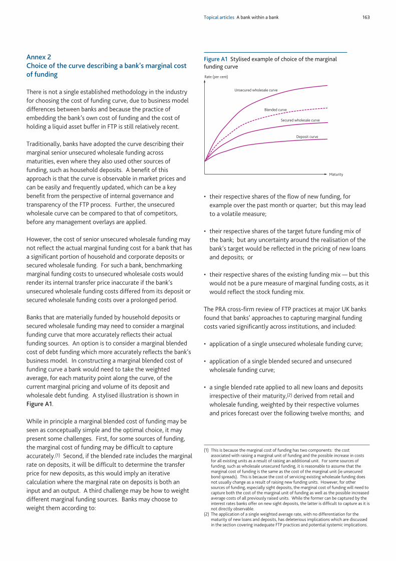
Topical articles A bank within a bank 163
Annex 2Choice of the curve describing a bank’s marginal costof funding
There is not a single established methodology in the industryfor choosing the cost of funding curve, due to business modeldifferences between banks and because the practice ofembedding the bank’s own cost of funding and the cost ofholding a liquid asset buffer in FTP is still relatively recent.
Traditionally, banks have adopted the curve describing theirmarginal senior unsecured wholesale funding acrossmaturities, even where they also used other sources offunding, such as household deposits. A benefit of thisapproach is that the curve is observable in market prices andcan be easily and frequently updated, which can be a keybenefit from the perspective of internal governance andtransparency of the FTP process. Further, the unsecuredwholesale curve can be compared to that of competitors,before any management overlays are applied.
However, the cost of senior unsecured wholesale funding maynot reflect the actual marginal funding cost for a bank that hasa significant portion of household and corporate deposits orsecured wholesale funding. For such a bank, benchmarkingmarginal funding costs to unsecured wholesale costs wouldrender its internal transfer price inaccurate if the bank’sunsecured wholesale funding costs differed from its deposit orsecured wholesale funding costs over a prolonged period.
Banks that are materially funded by household deposits orsecured wholesale funding may need to consider a marginalfunding curve that more accurately reflects their actualfunding sources. An option is to consider a marginal blendedcost of debt funding which more accurately reflects the bank’sbusiness model. In constructing a marginal blended cost offunding curve a bank would need to take the weightedaverage, for each maturity point along the curve, of thecurrent marginal pricing and volume of its deposit andwholesale debt funding. A stylised illustration is shown inFigure A1.
While in principle a marginal blended cost of funding may beseen as conceptually simple and the optimal choice, it maypresent some challenges. First, for some sources of funding,the marginal cost of funding may be difficult to captureaccurately.(1) Second, if the blended rate includes the marginalrate on deposits, it will be difficult to determine the transferprice for new deposits, as this would imply an iterativecalculation where the marginal rate on deposits is both aninput and an output. A third challenge may be how to weightdifferent marginal funding sources. Banks may choose toweight them according to:
• their respective shares of the flow of new funding, forexample over the past month or quarter; but this may leadto a volatile measure;
• their respective shares of the target future funding mix ofthe bank; but any uncertainty around the realisation of thebank’s target would be reflected in the pricing of new loansand deposits; or
• their respective shares of the existing funding mix — but thiswould not be a pure measure of marginal funding costs, as itwould reflect the stock funding mix.
The PRA cross-firm review of FTP practices at major UK banksfound that banks’ approaches to capturing marginal fundingcosts varied significantly across institutions, and included:
• application of a single unsecured wholesale funding curve;
• application of a single blended secured and unsecuredwholesale funding curve;
• a single blended rate applied to all new loans and depositsirrespective of their maturity,(2) derived from retail andwholesale funding, weighted by their respective volumesand prices forecast over the following twelve months; and
Deposit curve
Unsecured wholesale curve
Blended curve
Secured wholesale curve
Maturity
Rate (per cent)
Figure A1 Stylised example of choice of the marginalfunding curve
(1) This is because the marginal cost of funding has two components: the costassociated with raising a marginal unit of funding and the possible increase in costsfor all existing units as a result of raising an additional unit. For some sources offunding, such as wholesale unsecured funding, it is reasonable to assume that themarginal cost of funding is the same as the cost of the marginal unit (ie unsecuredbond spreads). This is because the cost of servicing existing wholesale funding doesnot usually change as a result of raising new funding units. However, for othersources of funding, especially sight deposits, the marginal cost of funding will need tocapture both the cost of the marginal unit of funding as well as the possible increasedaverage costs of all previously raised units. While the former can be captured by theinterest rates banks offer on new sight deposits, the latter is difficult to capture as it isnot directly observable.
(2) The application of a single weighted average rate, with no differentiation for thematurity of new loans and deposits, has deleterious implications which are discussedin the section covering inadequate FTP practices and potential systemic implications.

164 Quarterly Bulletin 2015 Q2
• a single blended rate applied to all new loans and depositsirrespective of their maturity, derived from retail, corporateand wholesale term funding costs, weighted against a targetfunding mix.
The trend towards using a blended cost of funding curve isconsistent with the latest Bank Liabilities Survey, where lendersreported that they put weight on different sources of fundingwhile setting their transfer prices.(1)
To sum up, banks’ different approaches to choosing thebenchmark funding curve reflect not only business model
differences but also the trade-off between practicality andaccuracy. Using the unsecured wholesale funding curve hasthe advantage that it is readily observable in market prices, akey benefit from the perspective of internal governance, eventhough it may not accurately reflect the actual marginal costof funding of the bank. Alternatively, using a blended marginalcost of funding would be more accurate, but thecorresponding curve may also be more complex to constructand less transparently anchored in market prices.
(1) See Bank Liabilities Survey, 2015 Q1, available atwww.bankofengland.co.uk/publications/Documents/other/monetary/bls/2015/q1.pdf.
References
Bailey, A, Breeden, S and Stevens, G (2012), ‘The Prudential Regulation Authority’, Bank of England Quarterly Bulletin, Vol. 52, No. 4,pages 354–62, available at www.bankofengland.co.uk/publications/Documents/quarterlybulletin/qb120405.pdf.
Beau, E, Hill, J, Hussain, T and Nixon, D (2014), ‘Bank funding costs: what are they, what determines them and why do they matter?’, Bank ofEngland Quarterly Bulletin, Vol. 54, No. 4, pages 370–84, available atwww.bankofengland.co.uk/publications/Documents/quarterlybulletin/2014/qb14q401.pdf.
Button, R, Pezzini, S and Rossiter, N (2010), ‘Understanding the price of new lending to households’, Bank of England Quarterly Bulletin,Vol. 50, No. 3, pages 172–82, available at www.bankofengland.co.uk/publications/Documents/quarterlybulletin/qb100301.pdf.
Murphy, E and Senior, S (2013), ‘Changes to the Bank of England’, Bank of England Quarterly Bulletin, Vol. 53, No. 1, pages 20–28, available atwww.bankofengland.co.uk/publications/Documents/quarterlybulletin/2013/qb130102.pdf.
Tucker, P, Hall, S and Pattani, A (2013), ‘Macroprudential policy at the Bank of England’, Bank of England Quarterly Bulletin, Vol. 53, No. 3,pages 192–200, available at www.bankofengland.co.uk/publications/Documents/quarterlybulletin/2013/qb130301.pdf.
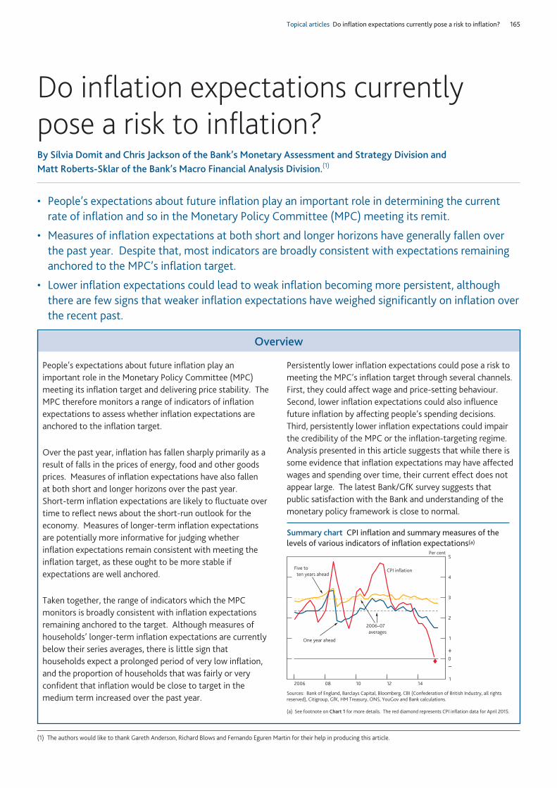
Topical articles Do inflation expectations currently pose a risk to inflation? 165
• People’s expectations about future inflation play an important role in determining the currentrate of inflation and so in the Monetary Policy Committee (MPC) meeting its remit.
• Measures of inflation expectations at both short and longer horizons have generally fallen overthe past year. Despite that, most indicators are broadly consistent with expectations remaininganchored to the MPC’s inflation target.
• Lower inflation expectations could lead to weak inflation becoming more persistent, althoughthere are few signs that weaker inflation expectations have weighed significantly on inflation overthe recent past.
Do inflation expectations currentlypose a risk to inflation?By Sílvia Domit and Chris Jackson of the Bank’s Monetary Assessment and Strategy Division and Matt Roberts-Sklar of the Bank’s Macro Financial Analysis Division.(1)
Overview
People’s expectations about future inflation play animportant role in the Monetary Policy Committee (MPC)meeting its inflation target and delivering price stability. TheMPC therefore monitors a range of indicators of inflationexpectations to assess whether inflation expectations areanchored to the inflation target.
Over the past year, inflation has fallen sharply primarily as aresult of falls in the prices of energy, food and other goodsprices. Measures of inflation expectations have also fallen at both short and longer horizons over the past year. Short-term inflation expectations are likely to fluctuate overtime to reflect news about the short-run outlook for theeconomy. Measures of longer-term inflation expectationsare potentially more informative for judging whetherinflation expectations remain consistent with meeting theinflation target, as these ought to be more stable ifexpectations are well anchored.
Taken together, the range of indicators which the MPCmonitors is broadly consistent with inflation expectationsremaining anchored to the target. Although measures ofhouseholds’ longer-term inflation expectations are currentlybelow their series averages, there is little sign thathouseholds expect a prolonged period of very low inflation,and the proportion of households that was fairly or veryconfident that inflation would be close to target in themedium term increased over the past year.
Persistently lower inflation expectations could pose a risk tomeeting the MPC’s inflation target through several channels.First, they could affect wage and price-setting behaviour.Second, lower inflation expectations could also influencefuture inflation by affecting people’s spending decisions.Third, persistently lower inflation expectations could impairthe credibility of the MPC or the inflation-targeting regime.Analysis presented in this article suggests that while there issome evidence that inflation expectations may have affectedwages and spending over time, their current effect does notappear large. The latest Bank/GfK survey suggests thatpublic satisfaction with the Bank and understanding of themonetary policy framework is close to normal.
1
0
1
2
3
4
5
2006 08 10 12 14
One year ahead
Five to ten years ahead
Per cent
2006–07 averages
CPI inflation
+
–
Summary chart CPI inflation and summary measures of thelevels of various indicators of inflation expectations(a)
Sources: Bank of England, Barclays Capital, Bloomberg, CBI (Confederation of British Industry, all rightsreserved), Citigroup, GfK, HM Treasury, ONS, YouGov and Bank calculations.
(a) See footnote on Chart 1 for more details. The red diamond represents CPI inflation data for April 2015.
(1) The authors would like to thank Gareth Anderson, Richard Blows and Fernando Eguren Martin for their help in producing this article.
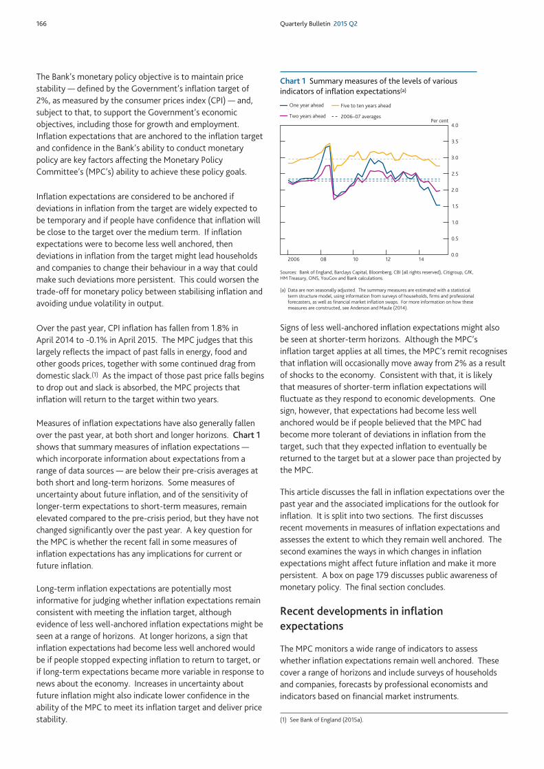
166 Quarterly Bulletin 2015 Q2
The Bank’s monetary policy objective is to maintain pricestability — defined by the Government’s inflation target of2%, as measured by the consumer prices index (CPI) — and,subject to that, to support the Government’s economicobjectives, including those for growth and employment.Inflation expectations that are anchored to the inflation targetand confidence in the Bank’s ability to conduct monetarypolicy are key factors affecting the Monetary PolicyCommittee’s (MPC’s) ability to achieve these policy goals.
Inflation expectations are considered to be anchored ifdeviations in inflation from the target are widely expected tobe temporary and if people have confidence that inflation willbe close to the target over the medium term. If inflationexpectations were to become less well anchored, thendeviations in inflation from the target might lead householdsand companies to change their behaviour in a way that couldmake such deviations more persistent. This could worsen thetrade-off for monetary policy between stabilising inflation andavoiding undue volatility in output.
Over the past year, CPI inflation has fallen from 1.8% in April 2014 to -0.1% in April 2015. The MPC judges that thislargely reflects the impact of past falls in energy, food andother goods prices, together with some continued drag fromdomestic slack.(1) As the impact of those past price falls beginsto drop out and slack is absorbed, the MPC projects thatinflation will return to the target within two years.
Measures of inflation expectations have also generally fallenover the past year, at both short and longer horizons. Chart 1shows that summary measures of inflation expectations —which incorporate information about expectations from arange of data sources — are below their pre-crisis averages atboth short and long-term horizons. Some measures ofuncertainty about future inflation, and of the sensitivity oflonger-term expectations to short-term measures, remainelevated compared to the pre-crisis period, but they have notchanged significantly over the past year. A key question forthe MPC is whether the recent fall in some measures ofinflation expectations has any implications for current orfuture inflation.
Long-term inflation expectations are potentially mostinformative for judging whether inflation expectations remainconsistent with meeting the inflation target, althoughevidence of less well-anchored inflation expectations might beseen at a range of horizons. At longer horizons, a sign thatinflation expectations had become less well anchored wouldbe if people stopped expecting inflation to return to target, orif long-term expectations became more variable in response tonews about the economy. Increases in uncertainty aboutfuture inflation might also indicate lower confidence in theability of the MPC to meet its inflation target and deliver pricestability.
Signs of less well-anchored inflation expectations might alsobe seen at shorter-term horizons. Although the MPC’sinflation target applies at all times, the MPC’s remit recognisesthat inflation will occasionally move away from 2% as a resultof shocks to the economy. Consistent with that, it is likelythat measures of shorter-term inflation expectations willfluctuate as they respond to economic developments. Onesign, however, that expectations had become less wellanchored would be if people believed that the MPC hadbecome more tolerant of deviations in inflation from thetarget, such that they expected inflation to eventually bereturned to the target but at a slower pace than projected bythe MPC.
This article discusses the fall in inflation expectations over thepast year and the associated implications for the outlook forinflation. It is split into two sections. The first discussesrecent movements in measures of inflation expectations andassesses the extent to which they remain well anchored. Thesecond examines the ways in which changes in inflationexpectations might affect future inflation and make it morepersistent. A box on page 179 discusses public awareness ofmonetary policy. The final section concludes.
Recent developments in inflationexpectations
The MPC monitors a wide range of indicators to assesswhether inflation expectations remain well anchored. Thesecover a range of horizons and include surveys of householdsand companies, forecasts by professional economists andindicators based on financial market instruments.
0.0
0.5
1.0
1.5
2.0
2.5
3.0
3.5
4.0
2006 08 10 12 14
One year ahead
Two years ahead
Five to ten years ahead
2006–07 averages Per cent
Sources: Bank of England, Barclays Capital, Bloomberg, CBI (all rights reserved), Citigroup, GfK,HM Treasury, ONS, YouGov and Bank calculations.
(a) Data are non seasonally adjusted. The summary measures are estimated with a statisticalterm structure model, using information from surveys of households, firms and professionalforecasters, as well as financial market inflation swaps. For more information on how thesemeasures are constructed, see Anderson and Maule (2014).
Chart 1 Summary measures of the levels of variousindicators of inflation expectations(a)
(1) See Bank of England (2015a).
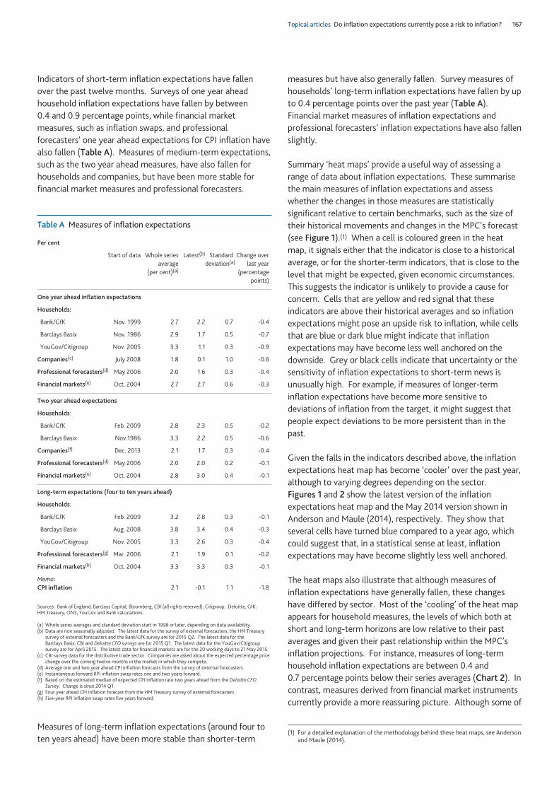
Topical articles Do inflation expectations currently pose a risk to inflation? 167
Indicators of short-term inflation expectations have fallen over the past twelve months. Surveys of one year aheadhousehold inflation expectations have fallen by between 0.4 and 0.9 percentage points, while financial marketmeasures, such as inflation swaps, and professionalforecasters’ one year ahead expectations for CPI inflation havealso fallen (Table A). Measures of medium-term expectations,such as the two year ahead measures, have also fallen forhouseholds and companies, but have been more stable forfinancial market measures and professional forecasters.
Measures of long-term inflation expectations (around four toten years ahead) have been more stable than shorter-term
measures but have also generally fallen. Survey measures ofhouseholds’ long-term inflation expectations have fallen by upto 0.4 percentage points over the past year (Table A).Financial market measures of inflation expectations andprofessional forecasters’ inflation expectations have also fallenslightly.
Summary ‘heat maps’ provide a useful way of assessing arange of data about inflation expectations. These summarisethe main measures of inflation expectations and assesswhether the changes in those measures are statisticallysignificant relative to certain benchmarks, such as the size oftheir historical movements and changes in the MPC’s forecast(see Figure 1).(1) When a cell is coloured green in the heatmap, it signals either that the indicator is close to a historicalaverage, or for the shorter-term indicators, that is close to thelevel that might be expected, given economic circumstances.This suggests the indicator is unlikely to provide a cause forconcern. Cells that are yellow and red signal that theseindicators are above their historical averages and so inflationexpectations might pose an upside risk to inflation, while cellsthat are blue or dark blue might indicate that inflationexpectations may have become less well anchored on thedownside. Grey or black cells indicate that uncertainty or thesensitivity of inflation expectations to short-term news isunusually high. For example, if measures of longer-terminflation expectations have become more sensitive todeviations of inflation from the target, it might suggest thatpeople expect deviations to be more persistent than in thepast.
Given the falls in the indicators described above, the inflationexpectations heat map has become ‘cooler’ over the past year,although to varying degrees depending on the sector. Figures 1 and 2 show the latest version of the inflationexpectations heat map and the May 2014 version shown inAnderson and Maule (2014), respectively. They show thatseveral cells have turned blue compared to a year ago, whichcould suggest that, in a statistical sense at least, inflationexpectations may have become slightly less well anchored.
The heat maps also illustrate that although measures ofinflation expectations have generally fallen, these changeshave differed by sector. Most of the ‘cooling’ of the heat mapappears for household measures, the levels of which both atshort and long-term horizons are low relative to their pastaverages and given their past relationship within the MPC’sinflation projections. For instance, measures of long-termhousehold inflation expectations are between 0.4 and 0.7 percentage points below their series averages (Chart 2). Incontrast, measures derived from financial market instrumentscurrently provide a more reassuring picture. Although some of
Table A Measures of inflation expectations
Per cent
Start of data Whole series Latest(b) Standard Change over average deviation(a) last year
(per cent)(a) (percentagepoints)
One year ahead inflation expectations
Households:
Bank/GfK Nov. 1999 2.7 2.2 0.7 -0.4
Barclays Basix Nov. 1986 2.9 1.7 0.5 -0.7
YouGov/Citigroup Nov. 2005 3.3 1.1 0.3 -0.9
Companies(c) July 2008 1.8 0.1 1.0 -0.6
Professional forecasters(d) May 2006 2.0 1.6 0.3 -0.4
Financial markets(e) Oct. 2004 2.7 2.7 0.6 -0.3
Two year ahead expectations
Households:
Bank/GfK Feb. 2009 2.8 2.3 0.5 -0.2
Barclays Basix Nov.1986 3.3 2.2 0.5 -0.6
Companies(f) Dec. 2013 2.1 1.7 0.3 -0.4
Professional forecasters(d) May 2006 2.0 2.0 0.2 -0.1
Financial markets(e) Oct. 2004 2.8 3.0 0.4 -0.1
Long-term expectations (four to ten years ahead)
Households:
Bank/GfK Feb. 2009 3.2 2.8 0.3 -0.1
Barclays Basix Aug. 2008 3.8 3.4 0.4 -0.3
YouGov/Citigroup Nov. 2005 3.3 2.6 0.3 -0.4
Professional forecasters(g) Mar. 2006 2.1 1.9 0.1 -0.2
Financial markets(h) Oct. 2004 3.3 3.3 0.3 -0.1
Memo:CPI inflation 2.1 -0.1 1.1 -1.8
Sources: Bank of England, Barclays Capital, Bloomberg, CBI (all rights reserved), Citigroup, Deloitte, GfK, HM Treasury, ONS, YouGov and Bank calculations.
(a) Whole series averages and standard deviation start in 1998 or later, depending on data availability.(b) Data are non seasonally adjusted. The latest data for the survey of external forecasters, the HM Treasury
survey of external forecasters and the Bank/GfK survey are for 2015 Q2. The latest data for the Barclays Basix, CBI and Deloitte CFO surveys are for 2015 Q1. The latest data for the YouGov/Citigroupsurvey are for April 2015. The latest data for financial markets are for the 20 working days to 21 May 2015.
(c) CBI survey data for the distributive trade sector. Companies are asked about the expected percentage pricechange over the coming twelve months in the market in which they compete.
(d) Average one and two year ahead CPI inflation forecasts from the survey of external forecasters.(e) Instantaneous forward RPI inflation swap rates one and two years forward. (f) Based on the estimated median of expected CPI inflation rate two years ahead from the Deloitte CFO
Survey. Change is since 2014 Q1. (g) Four year ahead CPI inflation forecast from the HM Treasury survey of external forecasters.(h) Five-year RPI inflation swap rates five years forward.
(1) For a detailed explanation of the methodology behind these heat maps, see Andersonand Maule (2014).
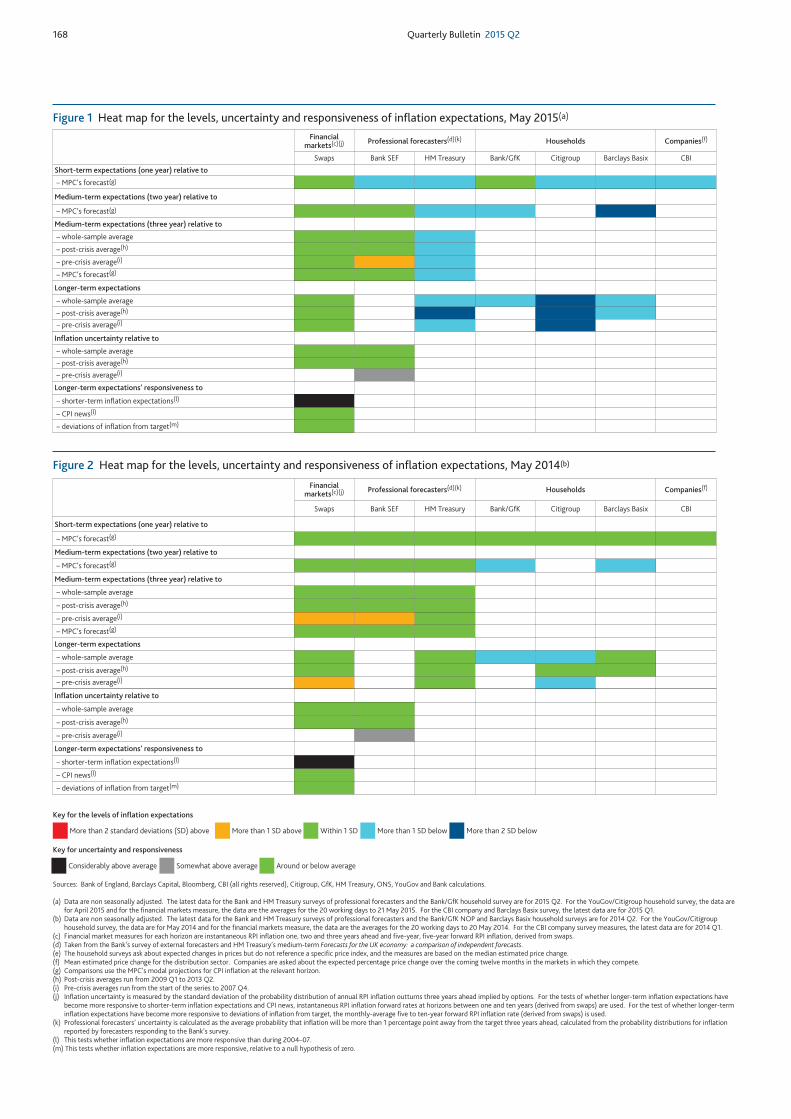
168 Quarterly Bulletin 2015 Q2
Financialmarkets(c)(j) Professional forecasters(d)(k) Households Companies(f)
Swaps Bank SEF HM Treasury Bank/GfK Citigroup Barclays Basix CBI
Short-term expectations (one year) relative to
– MPC’s forecast(g)
Medium-term expectations (two year) relative to
– MPC’s forecast(g)
Medium-term expectations (three year) relative to
– whole-sample average
– post-crisis average(h)
– pre-crisis average(i)
– MPC’s forecast(g)
Longer-term expectations
– whole-sample average
– post-crisis average(h)
– pre-crisis average(i)
Figure 1 Heat map for the levels, uncertainty and responsiveness of inflation expectations, May 2015(a)
Inflation uncertainty relative to
– whole-sample average
– post-crisis average(h)
– pre-crisis average(i)
Longer-term expectations’ responsiveness to
– shorter-term inflation expectations(l)
– CPI news(l)
– deviations of inflation from target(m)
Financialmarkets(c)(j) Professional forecasters(d)(k) Households Companies(f)
Swaps Bank SEF HM Treasury Bank/GfK Citigroup Barclays Basix CBI
Short-term expectations (one year) relative to
– MPC’s forecast(g)
Medium-term expectations (two year) relative to
– MPC’s forecast(g)
Medium-term expectations (three year) relative to
– whole-sample average
– post-crisis average(h)
– pre-crisis average(i)
– MPC’s forecast(g)
Longer-term expectations
– whole-sample average
– post-crisis average(h)
– pre-crisis average(i)
Figure 2 Heat map for the levels, uncertainty and responsiveness of inflation expectations, May 2014(b)
Inflation uncertainty relative to
– whole-sample average
– post-crisis average(h)
– pre-crisis average(i)
Longer-term expectations’ responsiveness to
– shorter-term inflation expectations(l)
– CPI news(l)
– deviations of inflation from target(m)
Sources: Bank of England, Barclays Capital, Bloomberg, CBI (all rights reserved), Citigroup, GfK, HM Treasury, ONS, YouGov and Bank calculations.
(a) Data are non seasonally adjusted. The latest data for the Bank and HM Treasury surveys of professional forecasters and the Bank/GfK household survey are for 2015 Q2. For the YouGov/Citigroup household survey, the data arefor April 2015 and for the financial markets measure, the data are the averages for the 20 working days to 21 May 2015. For the CBI company and Barclays Basix survey, the latest data are for 2015 Q1.
(b) Data are non seasonally adjusted. The latest data for the Bank and HM Treasury surveys of professional forecasters and the Bank/GfK NOP and Barclays Basix household surveys are for 2014 Q2. For the YouGov/Citigrouphousehold survey, the data are for May 2014 and for the financial markets measure, the data are the averages for the 20 working days to 20 May 2014. For the CBI company survey measures, the latest data are for 2014 Q1.
(c) Financial market measures for each horizon are instantaneous RPI inflation one, two and three years ahead and five-year, five-year forward RPI inflation, derived from swaps.(d) Taken from the Bank’s survey of external forecasters and HM Treasury’s medium-term Forecasts for the UK economy: a comparison of independent forecasts.(e) The household surveys ask about expected changes in prices but do not reference a specific price index, and the measures are based on the median estimated price change.(f) Mean estimated price change for the distribution sector. Companies are asked about the expected percentage price change over the coming twelve months in the markets in which they compete.(g) Comparisons use the MPC’s modal projections for CPI inflation at the relevant horizon.(h) Post-crisis averages run from 2009 Q1 to 2013 Q2.(i) Pre-crisis averages run from the start of the series to 2007 Q4.(j) Inflation uncertainty is measured by the standard deviation of the probability distribution of annual RPI inflation outturns three years ahead implied by options. For the tests of whether longer-term inflation expectations have
become more responsive to shorter-term inflation expectations and CPI news, instantaneous RPI inflation forward rates at horizons between one and ten years (derived from swaps) are used. For the test of whether longer-terminflation expectations have become more responsive to deviations of inflation from target, the monthly-average five to ten-year forward RPI inflation rate (derived from swaps) is used.
(k) Professional forecasters’ uncertainty is calculated as the average probability that inflation will be more than 1 percentage point away from the target three years ahead, calculated from the probability distributions for inflationreported by forecasters responding to the Bank’s survey.
(l) This tests whether inflation expectations are more responsive than during 2004–07.(m) This tests whether inflation expectations are more responsive, relative to a null hypothesis of zero.
More than 2 standard deviations (SD) above More than 1 SD above Within 1 SD
Key for the levels of inflation expectations
Considerably above average Somewhat above average Around or below average
More than 1 SD below More than 2 SD below
Key for uncertainty and responsiveness
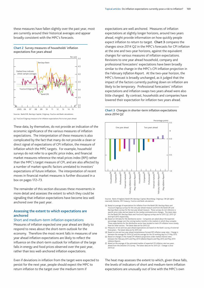
Topical articles Do inflation expectations currently pose a risk to inflation? 169
these measures have fallen slightly over the past year, mostare currently around their historical averages and appearbroadly consistent with the MPC’s forecasts.
These data, by themselves, do not provide an indication of theeconomic significance of the various measures of inflationexpectations. The interpretation of these measures is alsocomplicated by the fact that many do not provide a clean ordirect signal of expectations of CPI inflation, the measure ofinflation which the MPC targets. For example, householdsurveys do not refer to a specific price index, and financialmarket measures reference the retail prices index (RPI) ratherthan the MPC’s target measure of CPI, and are also affected bya number of market-specific factors unrelated to investors’expectations of future inflation. The interpretation of recentmoves in financial market measures is further discussed in abox on pages 172–73.
The remainder of this section discusses these movements inmore detail and assesses the extent to which they could besignalling that inflation expectations have become less wellanchored over the past year.
Assessing the extent to which expectations areanchoredShort and medium-term inflation expectationsMeasures of inflation expected one year ahead are likely torespond to news about the short-term outlook for theeconomy. Therefore the most recent falls in measures of oneyear ahead inflation expectations are likely to reflect theinfluence on the short-term outlook for inflation of the largefalls in energy and food prices observed over the past year,rather than less well-anchored inflation expectations.
Even if deviations in inflation from the target were expected topersist for the next year, people should expect the MPC toreturn inflation to the target over the medium term if
expectations are well anchored. Measures of inflationexpectations at slightly longer horizons, around two yearsahead, might provide information on how quickly peopleexpect inflation to return to target. Chart 3 compares thechanges since 2014 Q2 in the MPC’s forecasts for CPI inflationat the one and two-year horizons, against the equivalentchanges for various measures of inflation expectations.Revisions to one year ahead household, company andprofessional forecasters’ expectations have been broadlysimilar to the change in the MPC’s CPI inflation projection inthe February Inflation Report. At the two-year horizon, theMPC’s forecast is broadly unchanged, as it judged that theimpact of the factors currently pushing down on inflation arelikely to be temporary. Professional forecasters’ inflationexpectations and inflation swaps two years ahead were alsolittle changed. By contrast, households and companies havelowered their expectation for inflation two years ahead.
The heat map assesses the extent to which, given these falls,the levels of indicators of short and medium-term inflationexpectations are unusually out of line with the MPC’s own
2.0
2.5
3.0
3.5
4.0
4.5
5.0
2005 06 07 08 09 10 11 12 13 14 15
YouGov/Citigroup(a)
Bank/GfK
Barclays Basix
Per cent
Dashed lines indicate whole-sample averages
0.0
Sources: Bank/GfK, Barclays Capital, Citigroup, YouGov and Bank calculations.
(a) YouGov/Citigroup measure is for inflation expectations five to ten years ahead.
Chart 2 Survey measures of households’ inflationexpectations five years ahead
1.0
0.5
0.0
0.5
One year ahead
Two years ahead
Percentage points
+
–
Hou
seho
lds(a
)
Com
pani
es(b
)
Prof
essi
onal
s(c)
Fina
ncia
l mar
kets
(d)
Febr
uary
Infla
tion
Repo
rt(e
)
May
Infla
tion
Repo
rt(e
)
Hou
seho
lds(a
)
Com
pani
es(f
)
Prof
essi
onal
s(c)
Fina
ncia
l mar
kets
(d)
Febr
uary
Infla
tion
Repo
rt(e
)
May
Infla
tion
Repo
rt(e
)
Sources: Bank of England, Bank/GfK, Barclays Capital, Bloomberg, Citigroup, CBI (all rightsreserved), Deloitte, HM Treasury, YouGov and Bank calculations.
(a) Based on average of expectations for inflation from the Bank/GfK, Barclays Basix andYouGov/Citigroup surveys for the one year ahead measure and from the Bank/GfK andBarclays Basix surveys for the two year ahead measure. These surveys do not reference aspecific price index and are based on the median estimated price changes. The latest datafor the Bank/GfK, Barclays Basix and YouGov/Citigroup surveys are for 2015 Q2, 2015 Q1and April 2015 respectively.
(b) Based on CBI data for the distributive sector. Companies are asked about the expectedpercentage change over the coming twelve months in the markets in which they compete.These expectations for the distributive sector have tended to track CPI inflation more closelythan for other sectors. The latest data are for 2015 Q1.
(c) Measures of one and two year ahead expectations are based on the Bank’s survey of externalforecasters. The latest data are for 2015 Q2.
(d) Based on one and two year ahead instantaneous forward RPI inflation swap rates. Change isbetween the average for 2014 Q2 and the average for the 20 working days to 21 May 2015.
(e) Based on changes in the modal CPI inflation projections under market interest rates between the February 2015 and May 2014 Inflation Reports and May 2015 and May 2014Inflation Reports.
(f) Based on the average of the estimated median of expected CPI inflation rate two yearsahead from the Deloitte CFO Survey. The latest data are for 2015 Q1. Change is since 2014 Q1.
Chart 3 Changes in shorter-term inflation expectationssince 2014 Q2
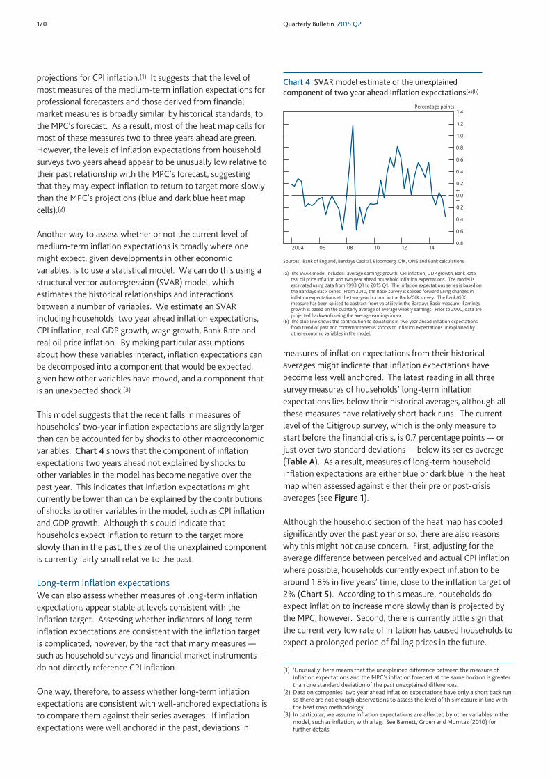
170 Quarterly Bulletin 2015 Q2
projections for CPI inflation.(1) It suggests that the level ofmost measures of the medium-term inflation expectations forprofessional forecasters and those derived from financialmarket measures is broadly similar, by historical standards, tothe MPC’s forecast. As a result, most of the heat map cells formost of these measures two to three years ahead are green.However, the levels of inflation expectations from householdsurveys two years ahead appear to be unusually low relative totheir past relationship with the MPC’s forecast, suggestingthat they may expect inflation to return to target more slowlythan the MPC’s projections (blue and dark blue heat mapcells).(2)
Another way to assess whether or not the current level ofmedium-term inflation expectations is broadly where onemight expect, given developments in other economicvariables, is to use a statistical model. We can do this using astructural vector autoregression (SVAR) model, whichestimates the historical relationships and interactions between a number of variables. We estimate an SVARincluding households’ two year ahead inflation expectations,CPI inflation, real GDP growth, wage growth, Bank Rate andreal oil price inflation. By making particular assumptionsabout how these variables interact, inflation expectations canbe decomposed into a component that would be expected,given how other variables have moved, and a component thatis an unexpected shock.(3)
This model suggests that the recent falls in measures ofhouseholds’ two-year inflation expectations are slightly largerthan can be accounted for by shocks to other macroeconomicvariables. Chart 4 shows that the component of inflationexpectations two years ahead not explained by shocks toother variables in the model has become negative over thepast year. This indicates that inflation expectations mightcurrently be lower than can be explained by the contributionsof shocks to other variables in the model, such as CPI inflationand GDP growth. Although this could indicate thathouseholds expect inflation to return to the target moreslowly than in the past, the size of the unexplained componentis currently fairly small relative to the past.
Long-term inflation expectationsWe can also assess whether measures of long-term inflationexpectations appear stable at levels consistent with theinflation target. Assessing whether indicators of long-terminflation expectations are consistent with the inflation targetis complicated, however, by the fact that many measures —such as household surveys and financial market instruments —do not directly reference CPI inflation.
One way, therefore, to assess whether long-term inflationexpectations are consistent with well-anchored expectations isto compare them against their series averages. If inflationexpectations were well anchored in the past, deviations in
measures of inflation expectations from their historicalaverages might indicate that inflation expectations havebecome less well anchored. The latest reading in all threesurvey measures of households’ long-term inflationexpectations lies below their historical averages, although allthese measures have relatively short back runs. The currentlevel of the Citigroup survey, which is the only measure tostart before the financial crisis, is 0.7 percentage points — orjust over two standard deviations — below its series average(Table A). As a result, measures of long-term householdinflation expectations are either blue or dark blue in the heatmap when assessed against either their pre or post-crisisaverages (see Figure 1).
Although the household section of the heat map has cooledsignificantly over the past year or so, there are also reasonswhy this might not cause concern. First, adjusting for theaverage difference between perceived and actual CPI inflationwhere possible, households currently expect inflation to bearound 1.8% in five years’ time, close to the inflation target of2% (Chart 5). According to this measure, households doexpect inflation to increase more slowly than is projected bythe MPC, however. Second, there is currently little sign thatthe current very low rate of inflation has caused households toexpect a prolonged period of falling prices in the future.
(1) ‘Unusually’ here means that the unexplained difference between the measure ofinflation expectations and the MPC’s inflation forecast at the same horizon is greaterthan one standard deviation of the past unexplained differences.
(2) Data on companies’ two year ahead inflation expectations have only a short back run,so there are not enough observations to assess the level of this measure in line withthe heat map methodology.
(3) In particular, we assume inflation expectations are affected by other variables in themodel, such as inflation, with a lag. See Barnett, Groen and Mumtaz (2010) forfurther details.
0.8
0.6
0.4
0.2
0.0
0.2
0.4
0.6
0.8
1.0
1.2
1.4
2004 06 08 10 12 14
Percentage points
+–
Sources: Bank of England, Barclays Capital, Bloomberg, GfK, ONS and Bank calculations.
(a) The SVAR model includes: average earnings growth, CPI inflation, GDP growth, Bank Rate,real oil price inflation and two year ahead household inflation expectations. The model isestimated using data from 1993 Q1 to 2015 Q1. The inflation expectations series is based onthe Barclays Basix series. From 2010, the Basix survey is spliced forward using changes ininflation expectations at the two-year horizon in the Bank/GfK survey. The Bank/GfKmeasure has been spliced to abstract from volatility in the Barclays Basix measure. Earningsgrowth is based on the quarterly average of average weekly earnings. Prior to 2000, data areprojected backwards using the average earnings index.
(b) The blue line shows the contribution to deviations in two year ahead inflation expectationsfrom trend of past and contemporaneous shocks to inflation expectations unexplained byother economic variables in the model.
Chart 4 SVAR model estimate of the unexplainedcomponent of two year ahead inflation expectations(a)(b)
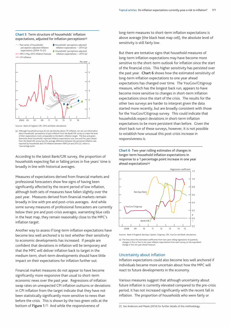
Topical articles Do inflation expectations currently pose a risk to inflation? 171
According to the latest Bank/GfK survey, the proportion ofhouseholds expecting flat or falling prices in five years’ time isbroadly in line with historical averages.
Measures of expectations derived from financial markets andprofessional forecasters show few signs of having beensignificantly affected by the recent period of low inflation,although both sets of measures have fallen slightly over thepast year. Measures derived from financial markets remainbroadly in line with pre and post-crisis averages. And whilesome survey measures of professional forecasters are currentlybelow their pre and post-crisis averages, warranting blue cellsin the heat map, they remain reasonably close to the MPC’sinflation target.
Another way to assess if long-term inflation expectations havebecome less well anchored is to test whether their sensitivityto economic developments has increased. If people areconfident that deviations in inflation will be temporary andthat the MPC will deliver inflation back to target in themedium term, short-term developments should have littleimpact on their expectations for inflation further out.
Financial market measures do not appear to have becomesignificantly more responsive than usual to short-termeconomic news over the past year. Regressions of inflationswap rates on unexpected CPI inflation outturns or deviationsin CPI inflation from the target indicate that they have notbeen statistically significantly more sensitive to news thanbefore the crisis. This is shown by the two green cells at thebottom of Figure 1.(1) And while the responsiveness of
long-term measures to short-term inflation expectations isabove average (the black heat map cell), the absolute level ofsensitivity is still fairly low.
But there are tentative signs that household measures of long-term inflation expectations may have become moresensitive to the short-term outlook for inflation since the startof the financial crisis. This higher sensitivity has persisted overthe past year. Chart 6 shows how the estimated sensitivity oflong-term inflation expectations to one year aheadexpectations has changed over time. The YouGov/Citigroupmeasure, which has the longest back run, appears to havebecome more sensitive to changes in short-term inflationexpectations since the start of the crisis. The results for theother two surveys are harder to interpret given the datastarted more recently, but are broadly consistent with thosefor the YouGov/Citigroup survey. This could indicate thathouseholds expect deviations in short-term inflationexpectations to be more persistent than before. Given theshort back run of these surveys, however, it is not possible to establish how unusual this post-crisis increase inresponsiveness is.
Uncertainty about inflationInflation expectations could also become less well anchored ifindividuals became more uncertain about how the MPC willreact to future developments in the economy.
Various measures suggest that although uncertainty aboutfuture inflation is currently elevated compared to the pre-crisisperiod, it has not increased significantly with the recent fall ininflation. The proportion of households who were fairly or
0
1
2
3
4
5
6
2003 05 07 09 11 13 15 17 19
Past series of households' perceptions-adjusted inflation expectations (2009–15 Q1)
Per cent
MPC’s May 2015 inflation forecastCPI inflation
Households’ perceptions-adjusted inflation expectations — 2014 Q2Households’ perceptions-adjusted inflation expectations — 2015 Q2
Sources: Bank of England, GfK, ONS and Bank calculations.
(a) Although household surveys do not ask directly about CPI inflation, we can use informationabout households’ perceptions of past inflation from the Bank/GfK survey to make the levelof their expectations more comparable to the Bank’s inflation target. The blue and greendiamonds show households’ reported inflation expectations one, two and five years aheadfrom the Bank/GfK survey less the average difference between the perceived inflation ratereported by households and CPI inflation between 1999 Q4 and 2015 Q1, which is 1 percentage point.
Chart 5 Term structure of households’ inflationexpectations, adjusted for inflation perceptions(a)
0.2
0.0
0.2
0.4
0.6
0.8
1.0
1.2
2008 09 10 11 12 13 14 15
YouGov/Citigroup
Bank/GfK
Barclays Basix
Regression coefficient
+
–
Sources: Bank of England, Barclays Capital, Citigroup, GfK, YouGov and Bank calculations.
(a) The lines show the estimated coefficients from two-year rolling regressions of quarterlychanges in five or five to ten-year inflation expectations from each survey on the equivalentchange in the one year ahead measure.
Chart 6 Two-year rolling estimates of changes in longer-term household inflation expectations inresponse to a 1 percentage point increase in one yearahead expectations(a)
(1) See Anderson and Maule (2014) for further details of this methodology.
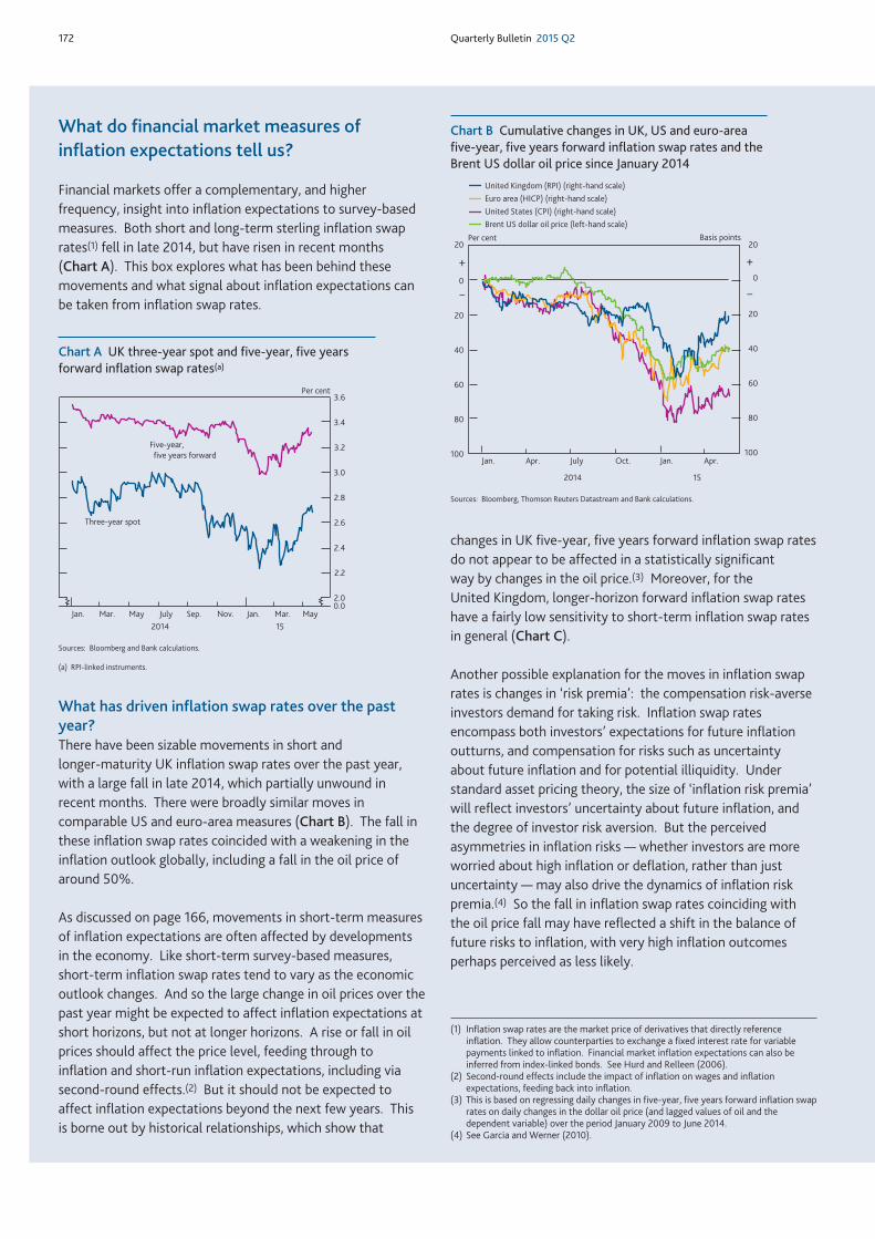
172 Quarterly Bulletin 2015 Q2
What do financial market measures ofinflation expectations tell us?
Financial markets offer a complementary, and higherfrequency, insight into inflation expectations to survey-basedmeasures. Both short and long-term sterling inflation swaprates(1) fell in late 2014, but have risen in recent months (Chart A). This box explores what has been behind thesemovements and what signal about inflation expectations canbe taken from inflation swap rates.
What has driven inflation swap rates over the pastyear?There have been sizable movements in short and longer-maturity UK inflation swap rates over the past year,with a large fall in late 2014, which partially unwound inrecent months. There were broadly similar moves incomparable US and euro-area measures (Chart B). The fall inthese inflation swap rates coincided with a weakening in theinflation outlook globally, including a fall in the oil price ofaround 50%.
As discussed on page 166, movements in short-term measuresof inflation expectations are often affected by developmentsin the economy. Like short-term survey-based measures,short-term inflation swap rates tend to vary as the economicoutlook changes. And so the large change in oil prices over thepast year might be expected to affect inflation expectations atshort horizons, but not at longer horizons. A rise or fall in oilprices should affect the price level, feeding through toinflation and short-run inflation expectations, including viasecond-round effects.(2) But it should not be expected toaffect inflation expectations beyond the next few years. Thisis borne out by historical relationships, which show that
changes in UK five-year, five years forward inflation swap ratesdo not appear to be affected in a statistically significant way by changes in the oil price.(3) Moreover, for the United Kingdom, longer-horizon forward inflation swap rateshave a fairly low sensitivity to short-term inflation swap ratesin general (Chart C).
Another possible explanation for the moves in inflation swaprates is changes in ‘risk premia’: the compensation risk-averseinvestors demand for taking risk. Inflation swap ratesencompass both investors’ expectations for future inflationoutturns, and compensation for risks such as uncertaintyabout future inflation and for potential illiquidity. Understandard asset pricing theory, the size of ‘inflation risk premia’will reflect investors’ uncertainty about future inflation, andthe degree of investor risk aversion. But the perceivedasymmetries in inflation risks — whether investors are moreworried about high inflation or deflation, rather than justuncertainty — may also drive the dynamics of inflation riskpremia.(4) So the fall in inflation swap rates coinciding withthe oil price fall may have reflected a shift in the balance offuture risks to inflation, with very high inflation outcomesperhaps perceived as less likely.
2.0
2.2
2.4
2.6
2.8
3.0
3.2
3.4
3.6
Jan. Mar. May July Sep. Nov. Jan. Mar. May
Three-year spot
Five-year, five years forward
Per cent
2014 15
0.0
Sources: Bloomberg and Bank calculations.
(a) RPI-linked instruments.
Chart A UK three-year spot and five-year, five yearsforward inflation swap rates(a)
United Kingdom (RPI) (right-hand scale)
United States (CPI) (right-hand scale) Euro area (HICP) (right-hand scale)
Brent US dollar oil price (left-hand scale)
100
80
60
40
20
0
20
100
80
60
40
20
0
20
Jan. Apr. July Oct. Jan. Apr.
Basis points Per cent
2014 15
+
–
+
–
Sources: Bloomberg, Thomson Reuters Datastream and Bank calculations.
Chart B Cumulative changes in UK, US and euro-areafive-year, five years forward inflation swap rates and theBrent US dollar oil price since January 2014
(1) Inflation swap rates are the market price of derivatives that directly referenceinflation. They allow counterparties to exchange a fixed interest rate for variablepayments linked to inflation. Financial market inflation expectations can also beinferred from index-linked bonds. See Hurd and Relleen (2006).
(2) Second-round effects include the impact of inflation on wages and inflationexpectations, feeding back into inflation.
(3) This is based on regressing daily changes in five-year, five years forward inflation swaprates on daily changes in the dollar oil price (and lagged values of oil and thedependent variable) over the period January 2009 to June 2014.
(4) See Garcia and Werner (2010).
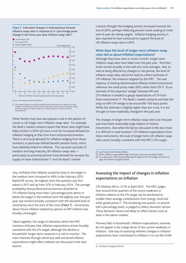
Topical articles Do inflation expectations currently pose a risk to inflation? 173
Other factors may have also played a role in the pattern ofmoves in UK longer-term inflation swap rates. For example,the Bank’s market contacts report that these rates might havefallen further in 2014 Q4 were it not for increased demand forinflation hedging at that time from institutional investors.There is structural demand for inflation hedging from theseinvestors, in particular defined benefit pension funds, whichhave liabilities linked to inflation. This can push up levels ofmedium and long-maturity UK inflation swap rates —particularly as potential pension fund demand far exceeds thesupply of index-linked bonds.(1) And the Bank’s market
contacts thought this hedging activity increased towards theend of 2014, perhaps reflecting pension funds seeking to meetend-of-year de-risking targets. Inflation hedging activity isalso reported to have continued to support the level of UK inflation swap rates in 2015.
What does the level of longer-term inflation swaprates tell us about inflation expectations?Although they have risen in recent months, longer-terminflation swap rates have fallen over the past year. And theirlevels remain broadly in line with pre-crisis averages. But, aswell as being affected by changes in risk premia, the level ofinflation swap rates cannot be read as a direct estimate of CPI inflation, the measure targeted by the MPC. The vastmajority of sterling-denominated inflation-linked instrumentsreference the retail prices index (RPI) rather than CPI.(2) So anestimate of the expected ‘wedge’ between RPI and CPI inflation is needed to gauge expectations of CPI fromthese instruments.(3) The Bank’s market contacts estimate thelong-run RPI-CPI wedge to be around 80–100 basis points.While this estimate is slightly higher than pre-crisis, it is notthought to have materially changed in the past year.
The changes in longer-term inflation swap rates over the pastyear have been reasonably large relative to historicmovements. But while the factors discussed in this box meanit is difficult to read investors’ CPI inflation expectations fromthese instruments, the level of longer-term UK inflation swaprates seems broadly consistent with the MPC’s 2% target.
0.00
0.05
0.10
0.15
0.20
0.25
0.30
0.35
0.40
0.45
0.50
4 5 6 7 8 9 10 11 12 13 14 15
United Kingdom (RPI)
United States (CPI) Euro area (HICP)
Horizon of inflation swap instantaneous forward rates (years)
Percentage points
Sources: Bloomberg and Bank calculations.
(a) The average changes are estimated using the slope coefficients from regressions of dailychanges in instantaneous inflation forward swap rates at each horizon on the daily change in the three-year spot inflation swap rate. Sample period is from January 2009 to December 2014.
Chart C Estimated changes in instantaneous forwardinflation swap rates in response to a 1 percentage pointchange in the three-year spot inflation swap rate(a)
(1) See McGrath and Windle (2006).(2) While inflation swaps referencing CPI do exist, they are not widely traded.(3) For a discussion of the factors affecting the long-run RPI-CPI wedge, see a box on
page 34 of Bank of England (2014).
very confident that inflation would be close to the target inthe medium term increased to 49% in the February 2015Bank/GfK survey, the highest since the question was firstasked in 2011 and up from 37% in February 2014. The averageprobability that professional economists attached to CPI inflation being more than 1 percentage point above orbelow the target in the medium term fell slightly over the pastyear, but remains broadly consistent with the elevated level ofuncertainty since the start of the crisis (Chart 7). Uncertaintyabout future inflation implied by options on RPI inflation wasbroadly unchanged.
Taken together, the range of indicators which the MPCmonitors indicates that inflation expectations remain broadlyconsistent with the 2% target, although the decline inhouseholds’ longer-term measures is a risk to monitor. Themain channels through which less well-anchored inflationexpectations might affect inflation are discussed in the nextsection.
Assessing the impact of changes in inflationexpectations on inflation
CPI inflation fell to -0.1% in April 2015. The MPC judges that around three quarters of the recent weakness in inflation relative to the 2% target can be attributed to smaller-than-average contributions from energy, food andother goods prices.(1) The remaining one quarter, or aroundhalf a percentage point, is judged to reflect domestic factors.These domestic factors are likely to reflect factors such asslack in the labour market.
Previous falls in households’ inflation expectations, however,do not appear to be a large driver of the current weakness ininflation. One way of assessing whether changes in inflationexpectations have contributed to inflation is to use the SVAR
(1) See Bank of England (2015a).
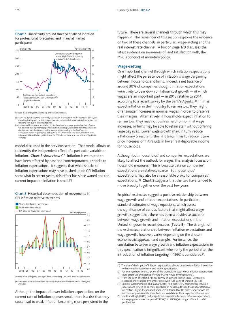
174 Quarterly Bulletin 2015 Q2
model discussed in the previous section. That model allows usto identify the independent effect of a particular variable oninflation. Chart 8 shows how CPI inflation is estimated tohave been affected by past and contemporaneous shocks toinflation expectations. It suggests that while shocks toinflation expectations may have pushed up on CPI inflationsomewhat in recent years, this effect has since waned and thecurrent impact on inflation is small.(1)
Although the impact of lower inflation expectations on thecurrent rate of inflation appears small, there is a risk that theycould lead to weak inflation becoming more persistent in the
future. There are several channels through which this mayhappen.(2) The remainder of this section explores the evidenceon two of these channels, in particular: wage-setting and thereal interest rate channel. A box on page 179 discusses thelatest evidence on awareness of, and satisfaction with, theMPC’s conduct of monetary policy.
Wage-settingOne important channel through which inflation expectationsmight affect the persistence of inflation is wage bargainingbetween households and firms. Indeed, a net balance ofaround 30% of companies thought inflation expectationswere likely to bear down on labour cost growth — of whichwages are an important part — in 2015 relative to 2014,according to a recent survey by the Bank’s Agents.(3) If firmsexpect inflation in their industry to remain low, they mightoffer smaller increases in nominal wages in order to preservetheir margins. Alternatively, if households expect inflation toremain low, they may not push as hard for nominal wageincreases, or firms may be able to retain staff without offeringlarge pay rises. Lower wage growth may, in turn, reduceinflationary pressure further if it leads firms to reduce futureprice increases or if it results in lower real disposable incomefor households.
Although both households’ and companies’ expectations arelikely to affect the outlook for wages, this analysis focuses onhousehold measures. This is because data on companies’expectations are relatively scarce. But households’expectations may also be a reasonable proxy for companies’expectations.(4) Chart 9 suggests that the two have tended tomove broadly together over the past few years.
Empirical estimates suggest a positive relationship betweenwage growth and inflation expectations. In particular,standard estimates of wage equations, which assess the significance of various factors that might affect wagegrowth, suggest that there has been a positive associationbetween wage growth and inflation expectations in the United Kingdom in recent decades (Table B). The strength ofthe estimated relationship between inflation expectations andwage growth, however, varies depending on the choseneconometric approach and sample. For instance, thecorrelation between wage growth and inflation expectations inthis specification is insignificant when only the period after theintroduction of inflation targeting in 1992 is considered.(5)
2.0
1.5
1.0
0.5
0.0
0.5
1.0
1.5
2.0
2.5
3.0
2004 05 06 07 08 09 10 11 12 13 14 15
Other economic shocks
Percentage points
+
–
Shocks to inflation expectations
CPI inflation deviations from trend
Sources: Bank of England, Barclays Capital, Bloomberg, GfK, ONS and Bank calculations.
(a) Deviations in CPI inflation from the model-implied trend over the period 1993 Q1 to 2015 Q1.
Chart 8 Historical decomposition of movements in CPI inflation relative to trend(a)
0
50
100
150
200
250
300
350
2004 05 06 07 08 09 10 11 12 13 14 150
5
10
15
20
25
30
35
Professional forecasters’ uncertainty around medium-term CPI inflation(b) (right-hand scale)
Uncertainty around three year ahead RPI inflation implied by options(a) (left-hand scale)
Basis points Percentage points
Sources: Bank of England, Bloomberg and Bank calculations.
(a) Standard deviation of the probability distribution of annual RPI inflation outturns three yearsahead implied by options. It is not possible to construct a full set of probability distributionsfor some days due to technical reasons.
(b) Professional forecasters’ uncertainty is calculated as the average probability that inflationwill be more than 1 percentage point away from the target, calculated from the probabilitydistributions for inflation reported by forecasters responding to the Bank’s survey.Forecasters’ reported probability distributions for CPI inflation two years ahead betweenFebruary 2004 and February 2006; and for CPI inflation three years ahead from May 2006onwards.
Chart 7 Uncertainty around three year ahead inflationfor professional forecasters and financial marketparticipants
(1) The size of the impact of inflation expectations shocks on current inflation is sensitiveto the identification scheme and model specification.
(2) For a comprehensive description of the channels through which inflation expectationscould affect the persistence of inflation, see Maule and Pugh (2013).
(3) From the Bank of England Agents’ survey on pay and labour costs. Companies’responses are weighted by number employed. See Bank of England (2015b).
(4) Coibion, Gorodnichenko and Kumar (2015) find that New Zealand firms’ inflationexpectations tended to be more like those of households than those of professionalforecasters. Bryan, Meyer and Parker (2014) found that US firms’ expectations arelike those of professionals when both are asked about their expected inflation rate.
(5) Maule and Pugh (2013) find a significant correlation between inflation expectationsand wage growth over the period 1993 Q1 to 2006 Q4, using a different modelspecification.
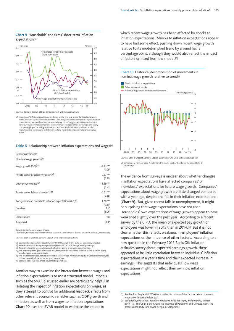
Topical articles Do inflation expectations currently pose a risk to inflation? 175
Another way to examine the interaction between wages andinflation expectations is to use a structural model. Modelssuch as the SVAR discussed earlier are particularly helpful inisolating the impact of inflation expectations on wages, asthey attempt to control for additional feedback effects fromother relevant economic variables such as GDP growth andinflation, as well as from wages to inflation expectations.Chart 10 uses the SVAR model to estimate the extent to
which recent wage growth has been affected by shocks toinflation expectations. Shocks to inflation expectations appearto have had some effect, pushing down recent wage growthrelative to its model-implied trend by around half apercentage point, although they would also reflect the impactof factors omitted from the model.(1)
The evidence from surveys is unclear about whether changesin inflation expectations have affected companies’ orindividuals’ expectations for future wage growth. Companies’expectations about wage growth are little changed comparedwith a year ago, despite the fall in their inflation expectations(Chart 9). But, given recent falls in unemployment, it mightbe surprising that wage expectations have not risen.Households’ own expectations of wage growth appear to haveweakened slightly over the past year. According to a recentsurvey by the CIPD, the mean of expected pay growth ofemployees was lower in 2015 than in 2014.(2) But it is notclear whether this reflects weakness in employees’ inflationexpectations or the influence of other factors. According to anew question in the February 2015 Bank/GfK inflationattitudes survey about expected earnings growth, thereappeared to be little correlation between individuals’ inflationexpectations in a year’s time and their expected increase inearnings. This suggests that individuals’ low wageexpectations might not reflect their own low inflationexpectations.
1.0
0.5
0.0
0.5
1.0
1.5
2.0
2.5
0.0
0.5
1.0
1.5
2.0
2.5
3.0
3.5
4.0
4.5
5.0
2008 09 10 11 12 13 14 15
Households’ inflation expectations (right-hand scale)
Firms’ wage expectations (right-hand scale)
Firms’ inflation expectations (left-hand scale)
Per centPer cent
+
–
Sources: Barclays Capital, CBI (all rights reserved) and Bank calculations.
(a) Households’ inflation expectations are based on the one year ahead Barclays Basix series.Firms’ inflation expectations are from the CBI surveys and reflect companies’ expectations ofprices twelve months ahead in their own industry. Firms’ wage expectations are from thesame survey and reflect companies’ expectations of changes in their own wages and salarycost per employee, including overtime and bonuses. Both CBI series are based on themanufacturing, services and distribution sectors, weighted using nominal shares in valueadded.
Chart 9 Households’ and firms’ short-term inflationexpectations(a)
Table B Relationship between inflation expectations and wages(a)
Dependent variable:
Nominal wage growth(b)
Wage growth (t–1)(b) -0.33***(0.09)
Private sector productivity growth(c) 0.37***(0.10)
Unemployment gap(d) -2.29***(0.41)
Private sector labour share (t–1)(e) -1.51***(0.38)
Two-year ahead household inflation expectations (t–1)(f) 1.28***(0.30)
Constant 1.65(1.06)
Observations 100
R-squared 0.45
Robust standard errors in parentheses. Three stars, two stars and one star denote statistical significance at the 1%, 5% and 10% levels, respectively.
Sources: Bank of England, Barclays Capital, ONS and Bank calculations.
(a) Estimated using quarterly data between 1990 Q1 and 2015 Q1. Data are seasonally adjusted.(b) Annualised quarter-on-quarter growth of private sector total average weekly earnings.(c) Annualised quarter-on-quarter growth of private sector gross value added per job.(d) The unemployment gap is defined as the unemployment rate minus the Bank staff's estimate of the
steady-state unemployment rate. (e) The private sector labour share is defined as total average weekly earnings by private sector employees,
divided by nominal market sector gross value added.(f) Barclays Basix two year ahead household expectations.
(1) See Bank of England (2015a) for a wider discussion of the factors behind the weakwage growth over the last year.
(2) See Employee outlook: focus on employee attitudes to pay and pensions, Winter2014–15. The CIPD is the Chartered Institute of Personnel and Development, theprofessional body for HR and people development.
8
6
4
2
0
2
4
Other economic shocks
Shocks to inflation expectations
Percentage points
2004 05 06 07 08 09 10 11 12 13 14 15
Nominal wage growth deviations from trend
+
–
Sources: Bank of England, Barclays Capital, Bloomberg, GfK, ONS and Bank calculations.
(a) Deviations in nominal wage growth from the model-implied trend over the period 1993 Q1to 2015 Q1.
Chart 10 Historical decomposition of movements innominal wage growth relative to trend(a)
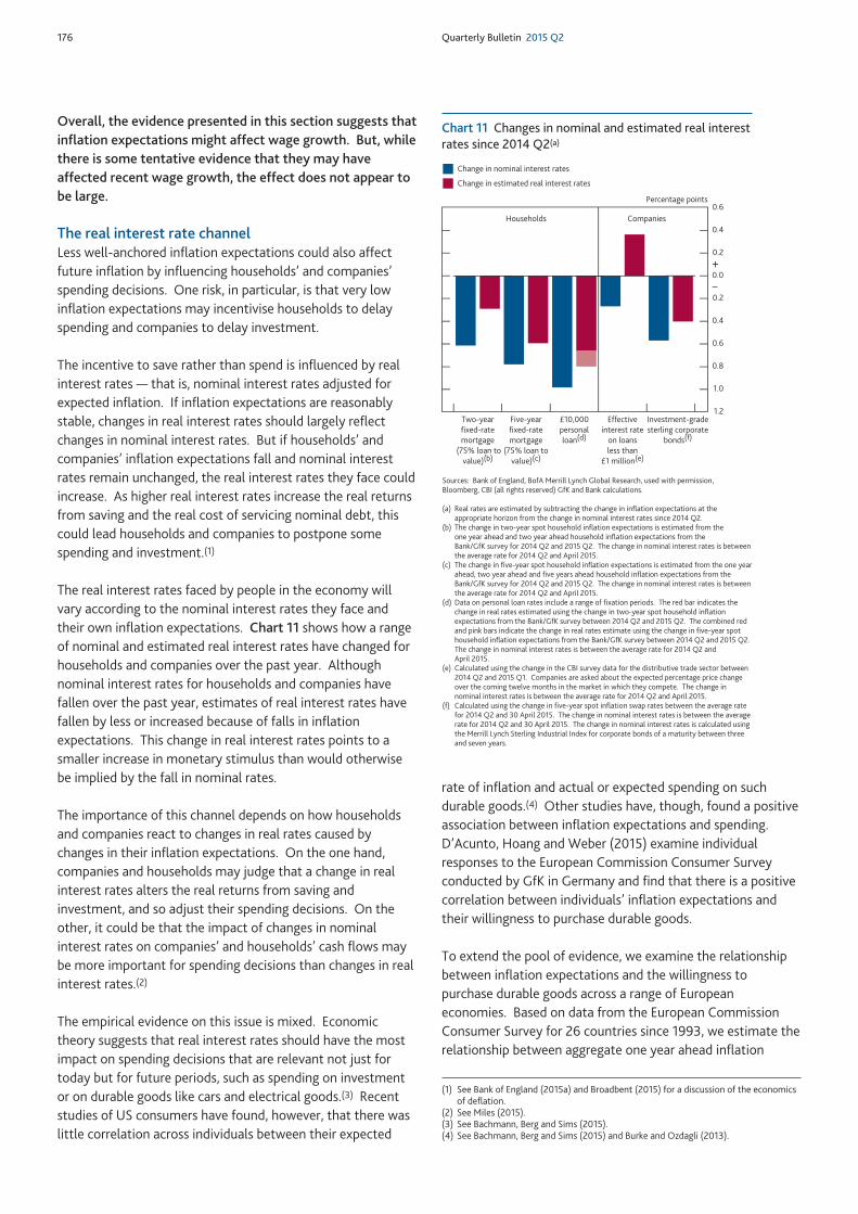
176 Quarterly Bulletin 2015 Q2
Overall, the evidence presented in this section suggests thatinflation expectations might affect wage growth. But, whilethere is some tentative evidence that they may haveaffected recent wage growth, the effect does not appear tobe large.
The real interest rate channelLess well-anchored inflation expectations could also affectfuture inflation by influencing households’ and companies’spending decisions. One risk, in particular, is that very lowinflation expectations may incentivise households to delayspending and companies to delay investment.
The incentive to save rather than spend is influenced by realinterest rates — that is, nominal interest rates adjusted forexpected inflation. If inflation expectations are reasonablystable, changes in real interest rates should largely reflectchanges in nominal interest rates. But if households’ andcompanies’ inflation expectations fall and nominal interestrates remain unchanged, the real interest rates they face couldincrease. As higher real interest rates increase the real returnsfrom saving and the real cost of servicing nominal debt, thiscould lead households and companies to postpone somespending and investment.(1)
The real interest rates faced by people in the economy willvary according to the nominal interest rates they face andtheir own inflation expectations. Chart 11 shows how a rangeof nominal and estimated real interest rates have changed forhouseholds and companies over the past year. Althoughnominal interest rates for households and companies havefallen over the past year, estimates of real interest rates havefallen by less or increased because of falls in inflationexpectations. This change in real interest rates points to asmaller increase in monetary stimulus than would otherwisebe implied by the fall in nominal rates.
The importance of this channel depends on how householdsand companies react to changes in real rates caused bychanges in their inflation expectations. On the one hand,companies and households may judge that a change in realinterest rates alters the real returns from saving andinvestment, and so adjust their spending decisions. On theother, it could be that the impact of changes in nominalinterest rates on companies’ and households’ cash flows maybe more important for spending decisions than changes in realinterest rates.(2)
The empirical evidence on this issue is mixed. Economictheory suggests that real interest rates should have the mostimpact on spending decisions that are relevant not just fortoday but for future periods, such as spending on investmentor on durable goods like cars and electrical goods.(3) Recentstudies of US consumers have found, however, that there waslittle correlation across individuals between their expected
rate of inflation and actual or expected spending on suchdurable goods.(4) Other studies have, though, found a positiveassociation between inflation expectations and spending.D’Acunto, Hoang and Weber (2015) examine individualresponses to the European Commission Consumer Surveyconducted by GfK in Germany and find that there is a positivecorrelation between individuals’ inflation expectations andtheir willingness to purchase durable goods.
To extend the pool of evidence, we examine the relationshipbetween inflation expectations and the willingness topurchase durable goods across a range of Europeaneconomies. Based on data from the European CommissionConsumer Survey for 26 countries since 1993, we estimate therelationship between aggregate one year ahead inflation
Percentage points
Change in nominal interest rates
Change in estimated real interest rates
Two-yearfixed-ratemortgage
(75% loan tovalue)(b)
Five-yearfixed-ratemortgage
(75% loan tovalue)(c)
£10,000personalloan(d)
Effectiveinterest rate
on loansless than
£1 million(e)
Investment-gradesterling corporate
bonds(f)
Households Companies
1.2
1.0
0.8
0.6
0.4
0.2
0.0
0.2
0.4
0.6
+
–
Sources: Bank of England, BofA Merrill Lynch Global Research, used with permission,Bloomberg, CBI (all rights reserved) GfK and Bank calculations.
(a) Real rates are estimated by subtracting the change in inflation expectations at theappropriate horizon from the change in nominal interest rates since 2014 Q2.
(b) The change in two-year spot household inflation expectations is estimated from the one year ahead and two year ahead household inflation expectations from the Bank/GfK survey for 2014 Q2 and 2015 Q2. The change in nominal interest rates is betweenthe average rate for 2014 Q2 and April 2015.
(c) The change in five-year spot household inflation expectations is estimated from the one yearahead, two year ahead and five years ahead household inflation expectations from theBank/GfK survey for 2014 Q2 and 2015 Q2. The change in nominal interest rates is betweenthe average rate for 2014 Q2 and April 2015.
(d) Data on personal loan rates include a range of fixation periods. The red bar indicates thechange in real rates estimated using the change in two-year spot household inflationexpectations from the Bank/GfK survey between 2014 Q2 and 2015 Q2. The combined redand pink bars indicate the change in real rates estimate using the change in five-year spothousehold inflation expectations from the Bank/GfK survey between 2014 Q2 and 2015 Q2.The change in nominal interest rates is between the average rate for 2014 Q2 and April 2015.
(e) Calculated using the change in the CBI survey data for the distributive trade sector between2014 Q2 and 2015 Q1. Companies are asked about the expected percentage price changeover the coming twelve months in the market in which they compete. The change innominal interest rates is between the average rate for 2014 Q2 and April 2015.
(f) Calculated using the change in five-year spot inflation swap rates between the average ratefor 2014 Q2 and 30 April 2015. The change in nominal interest rates is between the averagerate for 2014 Q2 and 30 April 2015. The change in nominal interest rates is calculated usingthe Merrill Lynch Sterling Industrial Index for corporate bonds of a maturity between threeand seven years.
Chart 11 Changes in nominal and estimated real interestrates since 2014 Q2(a)
(1) See Bank of England (2015a) and Broadbent (2015) for a discussion of the economicsof deflation.
(2) See Miles (2015).(3) See Bachmann, Berg and Sims (2015).(4) See Bachmann, Berg and Sims (2015) and Burke and Ozdagli (2013).
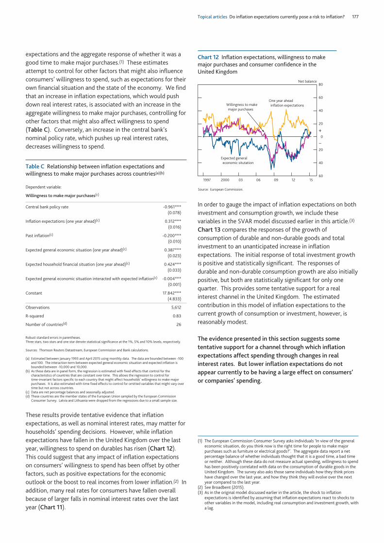
Topical articles Do inflation expectations currently pose a risk to inflation? 177
expectations and the aggregate response of whether it was agood time to make major purchases.(1) These estimatesattempt to control for other factors that might also influenceconsumers’ willingness to spend, such as expectations for theirown financial situation and the state of the economy. We findthat an increase in inflation expectations, which would pushdown real interest rates, is associated with an increase in theaggregate willingness to make major purchases, controlling forother factors that might also affect willingness to spend (Table C). Conversely, an increase in the central bank’snominal policy rate, which pushes up real interest rates,decreases willingness to spend.
These results provide tentative evidence that inflationexpectations, as well as nominal interest rates, may matter forhouseholds’ spending decisions. However, while inflationexpectations have fallen in the United Kingdom over the lastyear, willingness to spend on durables has risen (Chart 12).This could suggest that any impact of inflation expectationson consumers’ willingness to spend has been offset by otherfactors, such as positive expectations for the economicoutlook or the boost to real incomes from lower inflation.(2) Inaddition, many real rates for consumers have fallen overallbecause of larger falls in nominal interest rates over the lastyear (Chart 11).
In order to gauge the impact of inflation expectations on bothinvestment and consumption growth, we include thesevariables in the SVAR model discussed earlier in this article.(3)
Chart 13 compares the responses of the growth ofconsumption of durable and non-durable goods and totalinvestment to an unanticipated increase in inflationexpectations. The initial response of total investment growthis positive and statistically significant. The responses ofdurable and non-durable consumption growth are also initiallypositive, but both are statistically significant for only onequarter. This provides some tentative support for a realinterest channel in the United Kingdom. The estimatedcontribution in this model of inflation expectations to thecurrent growth of consumption or investment, however, isreasonably modest.
The evidence presented in this section suggests sometentative support for a channel through which inflationexpectations affect spending through changes in realinterest rates. But lower inflation expectations do notappear currently to be having a large effect on consumers’or companies’ spending.
Table C Relationship between inflation expectations andwillingness to make major purchases across countries(a)(b)
Dependent variable:
Willingness to make major purchases(c)
Central bank policy rate -0.961***(0.078)
Inflation expectations (one year ahead)(c) 0.312***(0.016)
Past inflation(c) -0.200***(0.010)
Expected general economic situation (one year ahead)(c) 0.387***(0.023)
Expected household financial situation (one year ahead)(c) 0.424***(0.033)
Expected general economic situation interacted with expected inflation(c) -0.004***(0.001)
Constant 17.842***(4.833)
Observations 5,612
R-squared 0.83
Number of countries(d) 26
Robust standard errors in parentheses.Three stars, two stars and one star denote statistical significance at the 1%, 5% and 10% levels, respectively.
Sources: Thomson Reuters Datastream, European Commission and Bank calculations.
(a) Estimated between January 1993 and April 2015 using monthly data. The data are bounded between -100and 100. The interaction term between expected general economic situation and expected inflation isbounded between -10,000 and 10,000.
(b) As these data are in panel form, the regression is estimated with fixed effects that control for thecharacteristics of countries that are constant over time. This allows the regression to control for time-invariant factors specific to each country that might affect households’ willingness to make majorpurchases. It is also estimated with time fixed effects to control for omitted variables that might vary overtime but not across countries.
(c) Data are net percentage balances and seasonally adjusted.(d) These countries are the member states of the European Union sampled by the European Commission
Consumer Survey. Latvia and Lithuania were dropped from the regressions due to a small sample size.
60
40
20
0
20
40
60
80
1997 2000 03 06 09 12 15
One year ahead inflation expectationsWillingness to make
major purchases
Expected general economic situtation
Net balance
+
–
Source: European Commission.
Chart 12 Inflation expectations, willingness to makemajor purchases and consumer confidence in the United Kingdom
(1) The European Commission Consumer Survey asks individuals ‘In view of the generaleconomic situation, do you think now is the right time for people to make majorpurchases such as furniture or electrical goods?’. The aggregate data report a netpercentage balance of whether individuals thought that it is a good time, a bad timeor neither. Although these data do not measure actual spending, willingness to spendhas been positively correlated with data on the consumption of durable goods in theUnited Kingdom. The survey also asks those same individuals how they think priceshave changed over the last year, and how they think they will evolve over the nextyear compared to the last year.
(2) See Broadbent (2015).(3) As in the original model discussed earlier in the article, the shock to inflation
expectations is identified by assuming that inflation expectations react to shocks toother variables in the model, including real consumption and investment growth, witha lag.
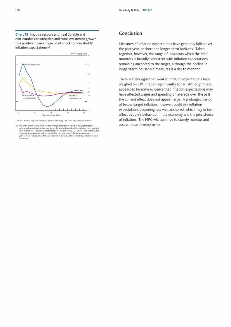
178 Quarterly Bulletin 2015 Q2
Conclusion
Measures of inflation expectations have generally fallen overthe past year, at short and longer-term horizons. Takentogether, however, the range of indicators which the MPCmonitors is broadly consistent with inflation expectationsremaining anchored to the target, although the decline inlonger-term household measures is a risk to monitor.
There are few signs that weaker inflation expectations haveweighed on CPI inflation significantly so far. Although thereappears to be some evidence that inflation expectations mayhave affected wages and spending on average over the past,the current effect does not appear large. A prolonged periodof below-target inflation, however, could risk inflationexpectations becoming less well anchored, which may in turnaffect people’s behaviour in the economy and the persistenceof inflation. The MPC will continue to closely monitor andassess these developments.
2
1
0
1
2
3
4
0 4 8 12 16
Durable consumption
Non-durable consumption
Total investment
Percentage points
Quarters after shock
+
–
Sources: Bank of England, Barclays Capital, Bloomberg, GfK, ONS and Bank calculations.
(a) This chart shows results from the same model described in Chart 4, but augmented toinclude real growth in the consumption of durable and non-durable goods and real growth intotal investment. The model is estimated over the period 1993 Q1 to 2014 Q4. It shows theimpact of a one-period shock to households’ two year ahead inflation expectations on year-on-year real growth in the consumption of durable and non-durable goods and in totalinvestment.
Chart 13 Impulse responses of real durable and non-durable consumption and total investment growthto a positive 1 percentage point shock to households’inflation expectations(a)
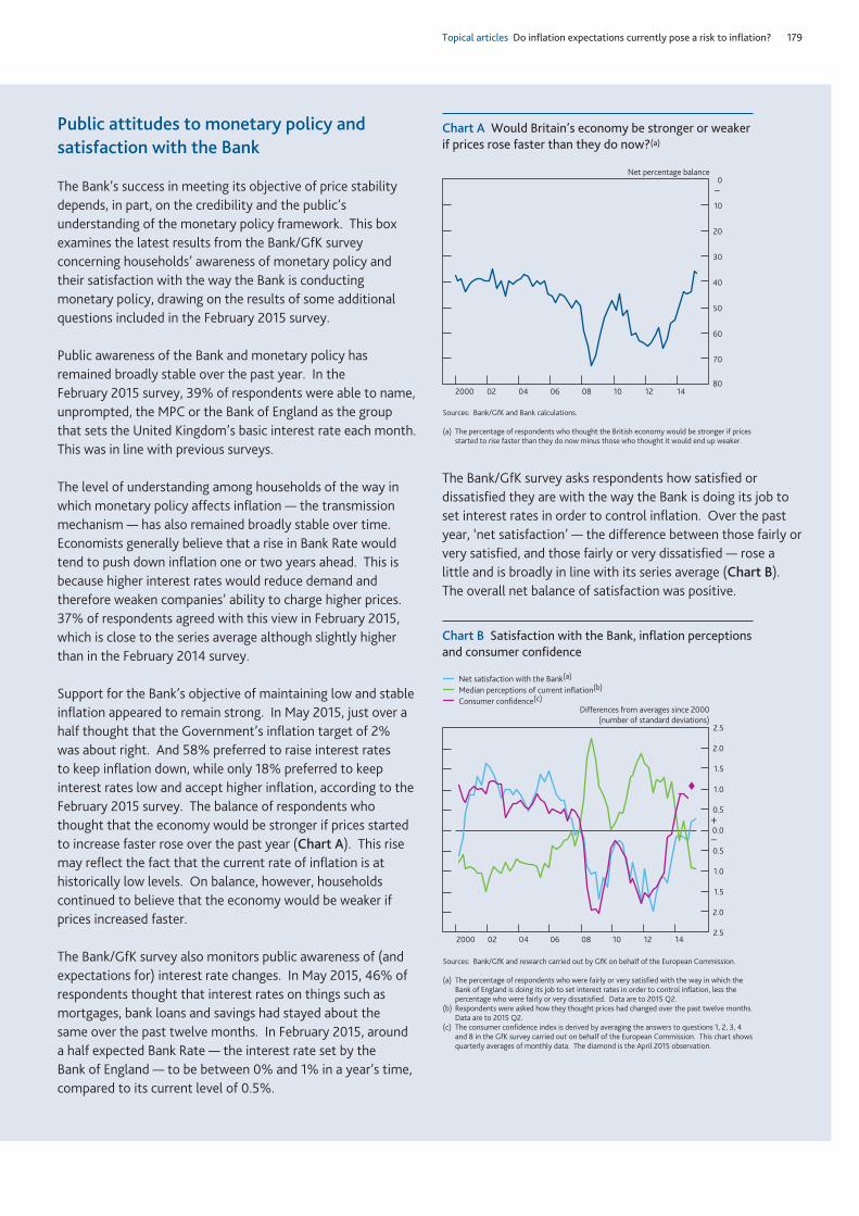
Topical articles Do inflation expectations currently pose a risk to inflation? 179
Public attitudes to monetary policy andsatisfaction with the Bank
The Bank’s success in meeting its objective of price stabilitydepends, in part, on the credibility and the public’sunderstanding of the monetary policy framework. This boxexamines the latest results from the Bank/GfK surveyconcerning households’ awareness of monetary policy andtheir satisfaction with the way the Bank is conductingmonetary policy, drawing on the results of some additionalquestions included in the February 2015 survey.
Public awareness of the Bank and monetary policy hasremained broadly stable over the past year. In the February 2015 survey, 39% of respondents were able to name,unprompted, the MPC or the Bank of England as the groupthat sets the United Kingdom’s basic interest rate each month.This was in line with previous surveys.
The level of understanding among households of the way inwhich monetary policy affects inflation — the transmissionmechanism — has also remained broadly stable over time.Economists generally believe that a rise in Bank Rate wouldtend to push down inflation one or two years ahead. This isbecause higher interest rates would reduce demand andtherefore weaken companies’ ability to charge higher prices.37% of respondents agreed with this view in February 2015,which is close to the series average although slightly higherthan in the February 2014 survey.
Support for the Bank’s objective of maintaining low and stableinflation appeared to remain strong. In May 2015, just over ahalf thought that the Government’s inflation target of 2% was about right. And 58% preferred to raise interest rates to keep inflation down, while only 18% preferred to keepinterest rates low and accept higher inflation, according to theFebruary 2015 survey. The balance of respondents whothought that the economy would be stronger if prices startedto increase faster rose over the past year (Chart A). This risemay reflect the fact that the current rate of inflation is athistorically low levels. On balance, however, householdscontinued to believe that the economy would be weaker ifprices increased faster.
The Bank/GfK survey also monitors public awareness of (andexpectations for) interest rate changes. In May 2015, 46% ofrespondents thought that interest rates on things such asmortgages, bank loans and savings had stayed about the same over the past twelve months. In February 2015, arounda half expected Bank Rate — the interest rate set by the Bank of England — to be between 0% and 1% in a year’s time,compared to its current level of 0.5%.
The Bank/GfK survey asks respondents how satisfied ordissatisfied they are with the way the Bank is doing its job toset interest rates in order to control inflation. Over the pastyear, ‘net satisfaction’ — the difference between those fairly orvery satisfied, and those fairly or very dissatisfied — rose alittle and is broadly in line with its series average (Chart B).The overall net balance of satisfaction was positive.
80
70
60
50
40
30
20
10
0
2000 02 04 06 08 10 12 14
Net percentage balance
–
Sources: Bank/GfK and Bank calculations.
(a) The percentage of respondents who thought the British economy would be stronger if pricesstarted to rise faster than they do now minus those who thought it would end up weaker.
Chart A Would Britain’s economy be stronger or weakerif prices rose faster than they do now?(a)
2.5
2.0
1.5
1.0
0.5
0.0
0.5
1.0
1.5
2.0
2.5
2000 02 04 06 08 10 12 14
Net satisfaction with the Bank(a) Median perceptions of current inflation(b)
Consumer confidence(c)Differences from averages since 2000
(number of standard deviations)
–
+
Sources: Bank/GfK and research carried out by GfK on behalf of the European Commission.
(a) The percentage of respondents who were fairly or very satisfied with the way in which theBank of England is doing its job to set interest rates in order to control inflation, less thepercentage who were fairly or very dissatisfied. Data are to 2015 Q2.
(b) Respondents were asked how they thought prices had changed over the past twelve months.Data are to 2015 Q2.
(c) The consumer confidence index is derived by averaging the answers to questions 1, 2, 3, 4and 8 in the GfK survey carried out on behalf of the European Commission. This chart showsquarterly averages of monthly data. The diamond is the April 2015 observation.
Chart B Satisfaction with the Bank, inflation perceptionsand consumer confidence

180 Quarterly Bulletin 2015 Q2
References
Anderson, G and Maule, B (2014), ‘Assessing the risk to inflation from inflation expectations’, Bank of England Quarterly Bulletin, Vol. 54, No. 2, pages 148–62, available at www.bankofengland.co.uk/publications/Documents/quarterlybulletin/2014/qb14q204.pdf.
Bachmann, R, Berg, T and Sims, E (2015), ‘Inflation expectations and readiness to spend: cross-sectional evidence’, American EconomicJournal: Economic Policy, Vol. 7, No. 1, pages 1–35.
Bank of England (2014), Inflation Report, February, available atwww.bankofengland.co.uk/publications/Documents/inflationreport/2014/ir14feb.pdf.
Bank of England (2015a), Inflation Report, May, available at www.bankofengland.co.uk/publications/Documents/inflationreport/2015/may.pdf.
Bank of England (2015b), Agents summary of business conditions, February, available atwww.bankofengland.co.uk/publications/Documents/agentssummary/2015/feb.pdf.
Barnett, A, Groen, J and Mumtaz, H (2010), ‘Time-varying inflation expectations and economic fluctuations in the United Kingdom: astructural VAR analysis’, Bank of England Working Paper No. 392, available atwww.bankofengland.co.uk/research/Documents/workingpapers/2010/wp392.pdf.
Broadbent, B (2015), ‘The economics of deflation’, available atwww.bankofengland.co.uk/publications/Documents/speeches/2015/speech813.pdf.
Bryan, M, Meyer, B and Parker, N (2014), ‘The inflation expectations of firms: what do they look like, are they accurate, and do they matter?’,Federal Reserve Bank of Atlanta Working Paper Series, No. 2014–27a.
Burke, M and Ozdagli, A (2013), ‘Household inflation expectations and consumer spending: evidence from panel data’, Federal Reserve Bank ofBoston Working Paper No. 13–25.
Coibion, O, Gorodnichenko, Y and Kumar, S (2015), ‘How do firms form their expectations? New survey evidence’, NBER Working Paper No. 21092.
D’Acunto, F, Hoang, D and Weber, M (2015), ‘Inflation expectations and consumption expenditure’, Chicago Booth Global Markets Working Paper Series.
Garcia, J A and Werner, T (2010), ‘Inflation risks and inflation risk premia’, European Central Bank Working Paper No. 1162.
Hurd, M and Relleen, J (2006), ‘New information from inflation swaps and index-linked bonds’, Bank of England Quarterly Bulletin, Spring,pages 24–34, available at www.bankofengland.co.uk/publications/Documents/quarterlybulletin/qb060101.pdf.
Maule, B and Pugh, A (2013), ‘Do inflation expectations currently pose a risk to the economy?’, Bank of England Quarterly Bulletin, Vol. 53, No. 2, pages 110–21, available at www.bankofengland.co.uk/publications/Documents/quarterlybulletin/2013/qb130202.pdf.
McGrath, G and Windle, R (2006), ‘Recent developments in sterling inflation-linked markets’, Bank of England Quarterly Bulletin, Vol. 46, No. 4, pages 386–96, available at www.bankofengland.co.uk/publications/Documents/quarterlybulletin/qb060402.pdf.
Miles, D (2015), ‘What can monetary policy do?’, available atwww.bankofengland.co.uk/publications/Documents/speeches/2015/speech791.pdf.
Topical articles Innovations in the Bank’s provision of liquidity insurance 181
• The Bank’s liquidity insurance facilities have been consistently improved since the onset of thefinancial crisis. The most innovative of these facilities is the Indexed Long-Term Repo (ILTR).
• In designing the ILTR, the Bank has drawn on lessons from auction theory. A key feature is thatthe provision of liquidity via the ILTR adjusts automatically to increases in demand caused byliquidity stresses in the financial system.
Innovations in the Bank’s provision ofliquidity insurance via IndexedLong-Term Repo (ILTR) operationsBy Tarkus Frost, Nick Govier and Tom Horn of the Bank’s Sterling Markets Division.(1)
Overview
The provision of liquidity insurance is a core function of theBank of England. It directly supports the Bank’s mission topromote the good of the people of the United Kingdom bymaintaining monetary and financial stability. The financialcrisis illustrated that, in times of stress, market participants’demand for liquidity insurance and the price they are willingto pay for it increases. The Bank, like other central banks,faced the challenge of needing to respond by providinglarge-scale liquidity insurance against a wide range ofcollateral.
Part of the Bank’s response included redesigning its existinglong-term repo operations, with the objective of increasingthe availability and flexibility of liquidity insurance provision.The operations now offer liquidity at longer maturitiesagainst the full range of Sterling Monetary Frameworkeligible collateral and at cheaper (auction-determined) rates.
Two automatic responses are now built into each IndexedLong-Term Repo (ILTR) operation. First, if the prices andquantities bid in the operation indicate that there are signs ofincreased stress on a particular set of collateral, a greaterproportion of the liquidity made available by the Bank is lentagainst that set. Second, the operation is no longer limitedto supplying a fixed quantity of liquidity. Instead, as thepattern of bids observed in the operation suggests a greateroverall demand, the total quantity of liquidity made availableis automatically increased. The allocation process achieves
this by maximising the combined ‘surplus’ of both producerand consumers as illustrated in the summary figure andexplained further in the annex.
Since the launch of the updated ILTR, demand for centralbank liquidity has been principally met with the reservessupplied by the Monetary Policy Committee’s assetpurchases, known as quantitative easing. However, asunconventional operations are wound down over time, theflexibility of the ILTR to respond to increased demand forliquidity, particularly in a market stress, is likely to prove avaluable addition to the Bank’s liquidity insurance toolkit.
Price
Quantity
Demand curve
Supply curve
Equilibrium quantity
Market price
Producer surplus
Consumer surplus
Summary figure The combined consumer and producersurplus
(1) The authors would like to thank Eleanor Broughton, David Elliott and Richard Gordonfor their help in producing this article, and are especially grateful to Professor PaulKlemperer who was instrumental in the design of the ILTR, and Dr Elizabeth Baldwinfor her help with the reforms.
182 Quarterly Bulletin 2015 Q2
The Bank of England’s mission is to promote the good of thepeople of the United Kingdom by maintaining monetary andfinancial stability. The Bank’s operations in the sterling moneymarkets, known as the Sterling Monetary Framework (SMF),serve that mission. They are designed to implement monetarypolicy and to support financial stability by acting as a backstopprovider of liquidity in order to reduce the cost of disruptionto critical financial services.
This article provides a brief overview of how the Bank’sprimary market-wide liquidity insurance tool, the IndexedLong-Term Repo (ILTR), has evolved from pre-crisis to thepresent day. It considers the liquidity risk that is a standardfeature of the banking system, and why central banks are wellplaced to act as backstop providers of liquidity. It thendescribes the steps that the Bank has taken to develop itsliquidity insurance operations, culminating in the reformsmade to the ILTR in February 2014. The article then goes onto demonstrate the two key features of the ILTR using anillustrative example.
Liquidity risk in the banking system
Banks, building societies and broker-dealers (henceforth‘banks’) are subject to liquidity risk: the risk that a materialpart of their funding is withdrawn before the assets they holdcan be realised at their true economic value. Liquidity risk is astandard feature of banking, and responsibility for managingnormal day-to-day fluctuations should fall to banksthemselves.
However, it is inefficient for banks to have to self-insureagainst extreme or ‘tail’ liquidity risks such as those caused bysudden market dysfunction. In such circumstances, centralbanks are well placed, as the monopoly suppliers of the mostliquid asset — central bank reserves — to act as backstopproviders of liquidity to solvent banks: so-called ‘liquidityinsurance’.
The Bank’s liquidity insurance facilities have been consistentlyimproved through a series of major reforms since the onset ofthe financial crisis. The most innovative of these facilities isthe Bank’s ILTR, a regular auction of central bank reserveswhich provides banks with an opportunity to obtain liquidityagainst a wide range of collateral.
In designing the ILTR the Bank has drawn on lessons fromauction theory. A key feature is that the provision of liquidityvia the ILTR adjusts automatically to increases in demand, forexample in the event of liquidity stresses in the financialsystem.
Evolution of the Bank’s liquidity insuranceprovision
Prior to the financial crisis, the Bank offered a limited amountof liquidity via monthly Long-Term Repo operations (LTRs) ata range of maturities. These fixed-size LTR auctions wereprimarily designed as a tool for the Bank to manage its balancesheet, by reducing the ‘churn’ of shorter-term liquiditysupplying operations used to implement monetary policy.The stock of lending via LTRs represented a relatively smallproportion of the overall quantity of liquidity supplied by theBank.
The auctions utilised a so-called ‘single-good’ auction format.Participants were able to bid to borrow central bank reservessecured against a single pool of highly liquid sovereign debtsecurities. A discriminatory pricing format was used, witheach successful bidder required to pay their bid price.Participants’ bids were ranked in descending order by price.Bids at the highest price were accepted first, followed by bidsat successively lower prices until all bids had been allocated infull, or the fixed total quantity of liquidity made available bythe Bank had been reached.
The first step towards the present ILTR operations was takentowards the end of 2007. In response to strains in fundingmarkets, demand for liquidity increased, particularly againstless liquid collateral. In response, the Bank announced asignificant expansion of its existing three-month Long-TermRepo operations, increasing the fixed total quantity of liquidityavailable and expanding the range of collateral accepted toinclude a wider range of less liquid, non-sovereign securitiesfor the first time.
These Extended Collateral Long-Term Repos (ELTRs) retainedthe same discriminatory price and single-good format used inthe earlier LTRs. However, in order to reflect the difference inliquidity between different types of collateral, a higherminimum bid rate was introduced for those participantswishing to borrow against the newly eligible, less liquidsecurities. As the crisis evolved, these ELTRs were offered ingreater size, at a greater frequency, and against a wider rangeof collateral. At their peak during January 2009, the stock ofoutstanding ELTRs reached £190 billion.
In June 2010 the ELTRs were replaced with ILTR operations, aspart of a move to make the eligibility of a broader range ofcollateral a permanent part of the SMF. Two ILTR auctionswith a three-month maturity and one with a six-monthmaturity were offered in each calendar quarter.
At this point a ‘multi-good’ auction format was adopted, withthe single pool of eligible collateral split into two distinct setsto better reflect their different liquidity characteristics — a
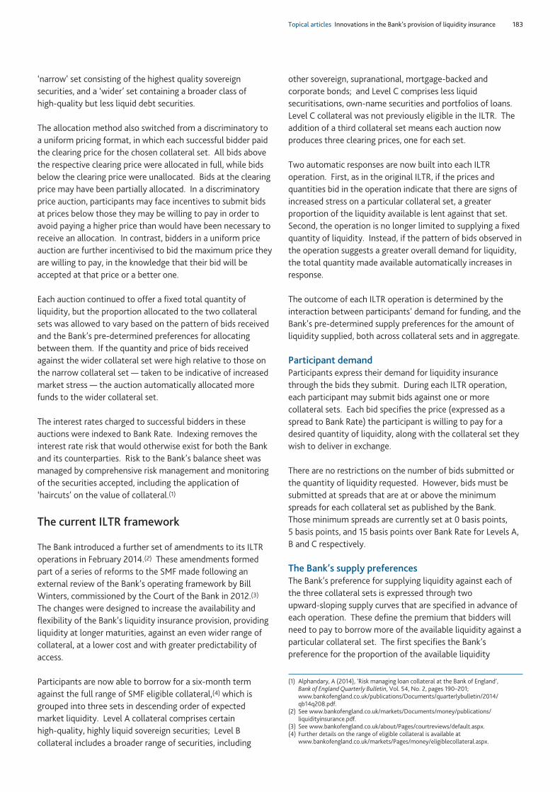
Topical articles Innovations in the Bank’s provision of liquidity insurance 183
‘narrow’ set consisting of the highest quality sovereignsecurities, and a ‘wider’ set containing a broader class ofhigh-quality but less liquid debt securities.
The allocation method also switched from a discriminatory toa uniform pricing format, in which each successful bidder paidthe clearing price for the chosen collateral set. All bids abovethe respective clearing price were allocated in full, while bidsbelow the clearing price were unallocated. Bids at the clearingprice may have been partially allocated. In a discriminatoryprice auction, participants may face incentives to submit bidsat prices below those they may be willing to pay in order toavoid paying a higher price than would have been necessary toreceive an allocation. In contrast, bidders in a uniform priceauction are further incentivised to bid the maximum price theyare willing to pay, in the knowledge that their bid will beaccepted at that price or a better one.
Each auction continued to offer a fixed total quantity ofliquidity, but the proportion allocated to the two collateralsets was allowed to vary based on the pattern of bids receivedand the Bank’s pre-determined preferences for allocatingbetween them. If the quantity and price of bids receivedagainst the wider collateral set were high relative to those onthe narrow collateral set — taken to be indicative of increasedmarket stress — the auction automatically allocated morefunds to the wider collateral set.
The interest rates charged to successful bidders in theseauctions were indexed to Bank Rate. Indexing removes theinterest rate risk that would otherwise exist for both the Bankand its counterparties. Risk to the Bank’s balance sheet wasmanaged by comprehensive risk management and monitoringof the securities accepted, including the application of‘haircuts’ on the value of collateral.(1)
The current ILTR framework
The Bank introduced a further set of amendments to its ILTRoperations in February 2014.(2) These amendments formedpart of a series of reforms to the SMF made following anexternal review of the Bank’s operating framework by BillWinters, commissioned by the Court of the Bank in 2012.(3)
The changes were designed to increase the availability andflexibility of the Bank’s liquidity insurance provision, providingliquidity at longer maturities, against an even wider range ofcollateral, at a lower cost and with greater predictability ofaccess.
Participants are now able to borrow for a six-month termagainst the full range of SMF eligible collateral,(4) which isgrouped into three sets in descending order of expectedmarket liquidity. Level A collateral comprises certainhigh-quality, highly liquid sovereign securities; Level Bcollateral includes a broader range of securities, including
other sovereign, supranational, mortgage-backed andcorporate bonds; and Level C comprises less liquidsecuritisations, own-name securities and portfolios of loans.Level C collateral was not previously eligible in the ILTR. Theaddition of a third collateral set means each auction nowproduces three clearing prices, one for each set.
Two automatic responses are now built into each ILTRoperation. First, as in the original ILTR, if the prices andquantities bid in the operation indicate that there are signs ofincreased stress on a particular collateral set, a greaterproportion of the liquidity available is lent against that set.Second, the operation is no longer limited to supplying a fixedquantity of liquidity. Instead, if the pattern of bids observed inthe operation suggests a greater overall demand for liquidity,the total quantity made available automatically increases inresponse.
The outcome of each ILTR operation is determined by theinteraction between participants’ demand for funding, and theBank’s pre-determined supply preferences for the amount ofliquidity supplied, both across collateral sets and in aggregate.
Participant demandParticipants express their demand for liquidity insurancethrough the bids they submit. During each ILTR operation,each participant may submit bids against one or morecollateral sets. Each bid specifies the price (expressed as aspread to Bank Rate) the participant is willing to pay for adesired quantity of liquidity, along with the collateral set theywish to deliver in exchange.
There are no restrictions on the number of bids submitted orthe quantity of liquidity requested. However, bids must besubmitted at spreads that are at or above the minimumspreads for each collateral set as published by the Bank.Those minimum spreads are currently set at 0 basis points,5 basis points, and 15 basis points over Bank Rate for Levels A,B and C respectively.
The Bank’s supply preferencesThe Bank’s preference for supplying liquidity against each ofthe three collateral sets is expressed through twoupward-sloping supply curves that are specified in advance ofeach operation. These define the premium that bidders willneed to pay to borrow more of the available liquidity against aparticular collateral set. The first specifies the Bank’spreference for the proportion of the available liquidity
(1) Alphandary, A (2014), ‘Risk managing loan collateral at the Bank of England’,Bank of England Quarterly Bulletin, Vol. 54, No. 2, pages 190–201;www.bankofengland.co.uk/publications/Documents/quarterlybulletin/2014/qb14q208.pdf.
(2) See www.bankofengland.co.uk/markets/Documents/money/publications/liquidityinsurance.pdf.
(3) See www.bankofengland.co.uk/about/Pages/courtreviews/default.aspx.(4) Further details on the range of eligible collateral is available at
www.bankofengland.co.uk/markets/Pages/money/eligiblecollateral.aspx.
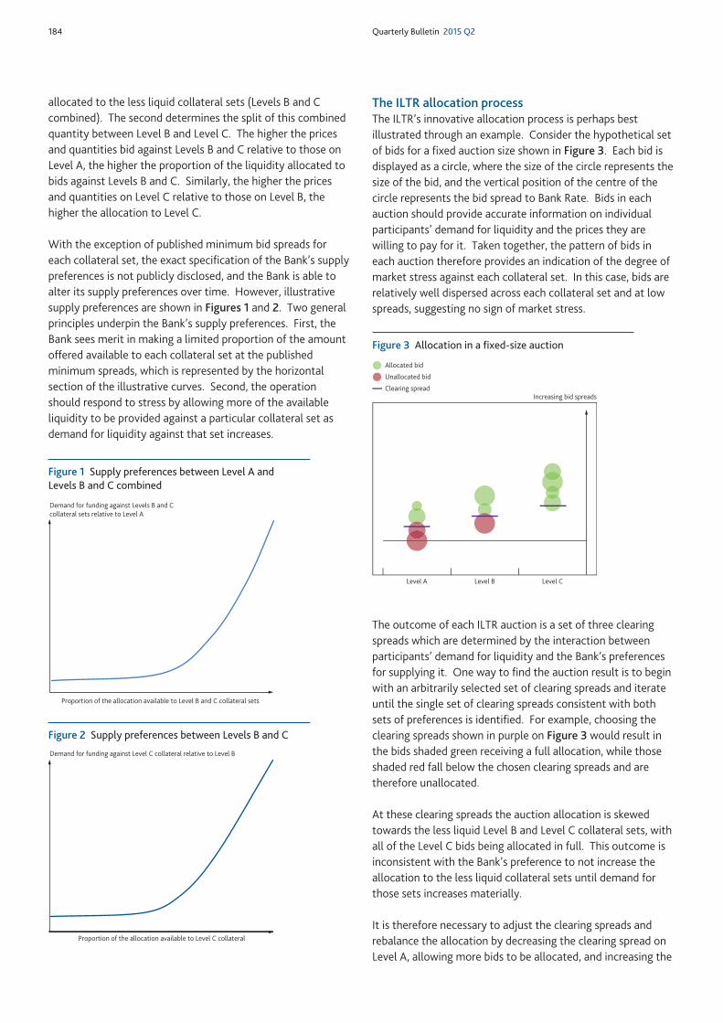
184 Quarterly Bulletin 2015 Q2
allocated to the less liquid collateral sets (Levels B and Ccombined). The second determines the split of this combinedquantity between Level B and Level C. The higher the pricesand quantities bid against Levels B and C relative to those onLevel A, the higher the proportion of the liquidity allocated tobids against Levels B and C. Similarly, the higher the pricesand quantities on Level C relative to those on Level B, thehigher the allocation to Level C.
With the exception of published minimum bid spreads foreach collateral set, the exact specification of the Bank’s supplypreferences is not publicly disclosed, and the Bank is able toalter its supply preferences over time. However, illustrativesupply preferences are shown in Figures 1 and 2. Two generalprinciples underpin the Bank’s supply preferences. First, theBank sees merit in making a limited proportion of the amountoffered available to each collateral set at the publishedminimum spreads, which is represented by the horizontalsection of the illustrative curves. Second, the operationshould respond to stress by allowing more of the availableliquidity to be provided against a particular collateral set asdemand for liquidity against that set increases.
The ILTR allocation processThe ILTR’s innovative allocation process is perhaps bestillustrated through an example. Consider the hypothetical setof bids for a fixed auction size shown in Figure 3. Each bid isdisplayed as a circle, where the size of the circle represents thesize of the bid, and the vertical position of the centre of thecircle represents the bid spread to Bank Rate. Bids in eachauction should provide accurate information on individualparticipants’ demand for liquidity and the prices they arewilling to pay for it. Taken together, the pattern of bids ineach auction therefore provides an indication of the degree ofmarket stress against each collateral set. In this case, bids arerelatively well dispersed across each collateral set and at lowspreads, suggesting no sign of market stress.
The outcome of each ILTR auction is a set of three clearingspreads which are determined by the interaction betweenparticipants’ demand for liquidity and the Bank’s preferencesfor supplying it. One way to find the auction result is to beginwith an arbitrarily selected set of clearing spreads and iterateuntil the single set of clearing spreads consistent with bothsets of preferences is identified. For example, choosing theclearing spreads shown in purple on Figure 3 would result inthe bids shaded green receiving a full allocation, while thoseshaded red fall below the chosen clearing spreads and aretherefore unallocated.
At these clearing spreads the auction allocation is skewedtowards the less liquid Level B and Level C collateral sets, withall of the Level C bids being allocated in full. This outcome isinconsistent with the Bank’s preference to not increase theallocation to the less liquid collateral sets until demand forthose sets increases materially.
It is therefore necessary to adjust the clearing spreads andrebalance the allocation by decreasing the clearing spread onLevel A, allowing more bids to be allocated, and increasing the
Demand for funding against Levels B and Ccollateral sets relative to Level A
Proportion of the allocation available to Level B and C collateral sets
Figure 1 Supply preferences between Level A andLevels B and C combined
Demand for funding against Level C collateral relative to Level B
Proportion of the allocation available to Level C collateral
Figure 2 Supply preferences between Levels B and C
Increasing bid spreads
Level A Level B Level C
Allocated bid
Unallocated bid
Clearing spread
Figure 3 Allocation in a fixed-size auction
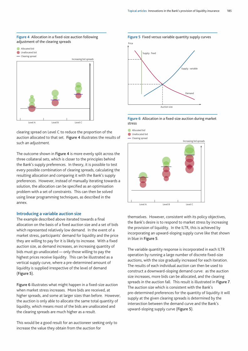
Topical articles Innovations in the Bank’s provision of liquidity insurance 185
clearing spread on Level C to reduce the proportion of theauction allocated to that set. Figure 4 illustrates the results ofsuch an adjustment.
The outcome shown in Figure 4 is more evenly split across thethree collateral sets, which is closer to the principles behindthe Bank’s supply preferences. In theory, it is possible to testevery possible combination of clearing spreads, calculating theresulting allocation and comparing it with the Bank’s supplypreferences. However, instead of manually iterating towards asolution, the allocation can be specified as an optimisationproblem with a set of constraints. This can then be solvedusing linear programming techniques, as described in theannex.
Introducing a variable auction sizeThe example described above iterated towards a finalallocation on the basis of a fixed auction size and a set of bidswhich represented relatively low demand. In the event of amarket stress, participants’ demand for liquidity and the pricethey are willing to pay for it is likely to increase. With a fixedauction size, as demand increases, an increasing quantity ofbids must go unallocated — only those willing to pay thehighest prices receive liquidity. This can be illustrated as avertical supply curve, where a pre-determined amount ofliquidity is supplied irrespective of the level of demand(Figure 5).
Figure 6 illustrates what might happen in a fixed-size auctionwhen market stress increases. More bids are received, athigher spreads, and some at larger sizes than before. However,the auction is only able to allocate the same total quantity ofliquidity, which means most of the bids are unallocated andthe clearing spreads are much higher as a result.
This would be a good result for an auctioneer seeking only toincrease the value they obtain from the auction for
themselves. However, consistent with its policy objectives,the Bank’s desire is to respond to market stress by increasingthe provision of liquidity. In the ILTR, this is achieved byincorporating an upward-sloping supply curve like that shownin blue in Figure 5.
The variable quantity response is incorporated in each ILTRoperation by running a large number of discrete fixed-sizeauctions, with the size gradually increased for each iteration.The results of each individual auction can then be used toconstruct a downward-sloping demand curve: as the auctionsize increases, more bids can be allocated, and the clearingspreads in the auction fall. This result is illustrated in Figure 7.The auction size which is consistent with the Bank’spre-determined preferences for the quantity of liquidity it willsupply at the given clearing spreads is determined by theintersection between the demand curve and the Bank’supward-sloping supply curve (Figure 5).
Increasing bid spreads
Level A Level B Level C
Allocated bid
Unallocated bid
Clearing spread
Figure 4 Allocation in a fixed-size auction followingadjustment of the clearing spreads
Increasing bid spreads
Level A Level B Level C
Allocated bid
Unallocated bid
Clearing spread
Figure 6 Allocation in a fixed-size auction during marketstress
Price
Auction size
Demand
Supply: fixed
Supply: variable
Figure 5 Fixed versus variable quantity supply curves
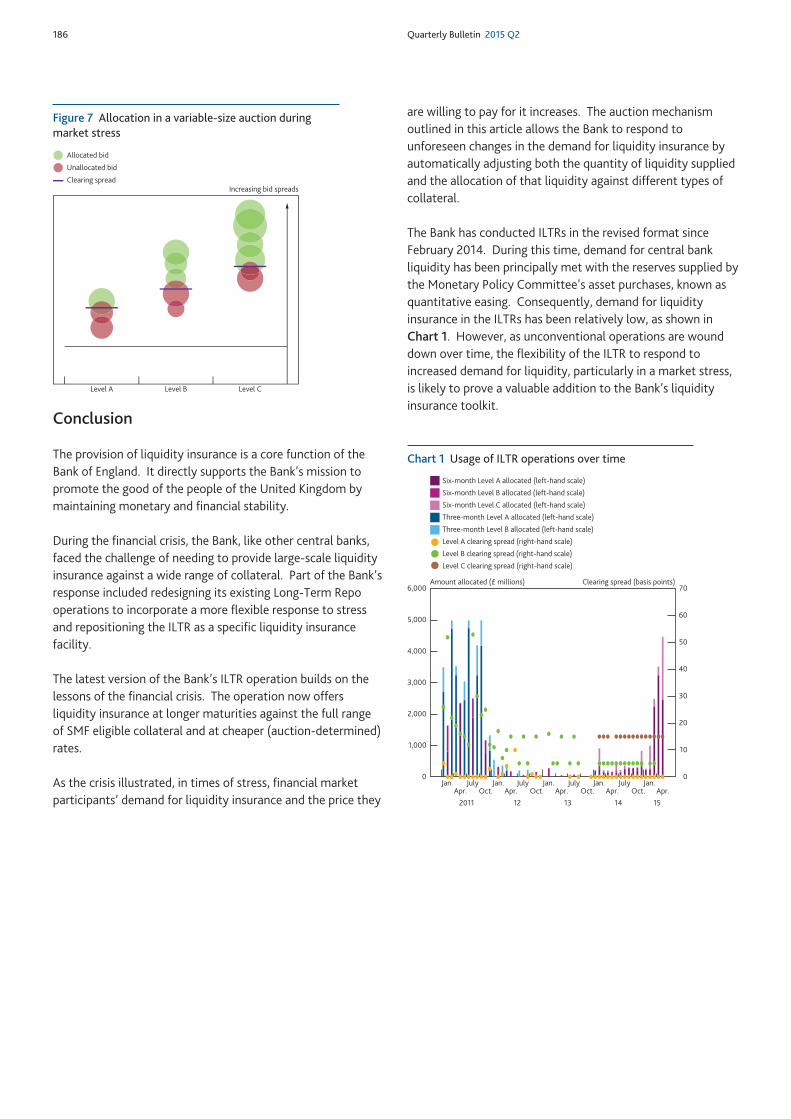
186 Quarterly Bulletin 2015 Q2
Conclusion
The provision of liquidity insurance is a core function of theBank of England. It directly supports the Bank’s mission topromote the good of the people of the United Kingdom bymaintaining monetary and financial stability.
During the financial crisis, the Bank, like other central banks,faced the challenge of needing to provide large-scale liquidityinsurance against a wide range of collateral. Part of the Bank’sresponse included redesigning its existing Long-Term Repooperations to incorporate a more flexible response to stressand repositioning the ILTR as a specific liquidity insurancefacility.
The latest version of the Bank’s ILTR operation builds on thelessons of the financial crisis. The operation now offersliquidity insurance at longer maturities against the full rangeof SMF eligible collateral and at cheaper (auction-determined)rates.
As the crisis illustrated, in times of stress, financial marketparticipants’ demand for liquidity insurance and the price they
are willing to pay for it increases. The auction mechanismoutlined in this article allows the Bank to respond tounforeseen changes in the demand for liquidity insurance byautomatically adjusting both the quantity of liquidity suppliedand the allocation of that liquidity against different types ofcollateral.
The Bank has conducted ILTRs in the revised format sinceFebruary 2014. During this time, demand for central bankliquidity has been principally met with the reserves supplied bythe Monetary Policy Committee’s asset purchases, known asquantitative easing. Consequently, demand for liquidityinsurance in the ILTRs has been relatively low, as shown inChart 1. However, as unconventional operations are wounddown over time, the flexibility of the ILTR to respond toincreased demand for liquidity, particularly in a market stress,is likely to prove a valuable addition to the Bank’s liquidityinsurance toolkit.
Increasing bid spreads
Level A Level B Level C
Allocated bid
Unallocated bid
Clearing spread
Figure 7 Allocation in a variable-size auction duringmarket stress
Jan.Apr.
JulyOct.
Jan.Apr.
JulyOct.
Jan.Apr.
Three-month Level A allocated (left-hand scale)
Three-month Level B allocated (left-hand scale)
Six-month Level A allocated (left-hand scale)
Six-month Level B allocated (left-hand scale)
Six-month Level C allocated (left-hand scale)
Level A clearing spread (right-hand scale)
Level B clearing spread (right-hand scale)
Level C clearing spread (right-hand scale)
Amount allocated (£ millions) Clearing spread (basis points)
0
1,000
2,000
3,000
4,000
5,000
6,000
0
10
20
30
40
50
60
70
2011 12 13 14 15
JulyOct.
Jan.Apr.
JulyOct.
Jan.Apr.
Chart 1 Usage of ILTR operations over time
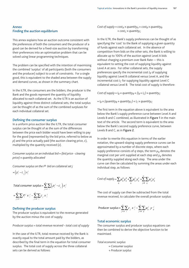
Topical articles Innovations in the Bank’s provision of liquidity insurance 187
AnnexFinding the auction equilibrium
This annex explains how an auction outcome consistent withthe preferences of both the consumers and the producer of agood can be derived for a fixed-size auction by transformingtheir preferences into an optimisation problem that can besolved using linear programming techniques.
The problem can be specified with the intention of maximisingthe combined ‘surplus’ of all participants (both the consumersand the producer) subject to a set of constraints. For a singlegood, this is equivalent to the shaded area between the supplyand demand curves, as shown in the summary chart.
In the ILTR, the consumers are the bidders, the producer is theBank and the goods represent the quantity of liquidityallocated to each collateral set. As the ILTR is an auction ofliquidity against three distinct collateral sets, the total surpluscan be thought of as the sum of the combined surpluses foreach individual collateral set.
Defining the consumer surplusIn a uniform price auction like the ILTR, the total consumersurplus can be thought of as the sum of the differencesbetween the price each bidder would have been willing to payfor the good (represented by the bid price, referred to below asp) and the price actually paid (the auction clearing price, c),multiplied by the quantity received (x).
Consumer surplus on an individual bid = (bid price - clearingprice) × quantity allocated
Consumer surplus on the ith bid on collateral set j
Defining the producer surplusThe producer surplus is equivalent to the revenue generatedby the auction minus the cost of supply.
Producer surplus = total revenue received – total cost of supply
In the case of the ILTR, total revenue received by the Bank isexactly equal to the total amount paid by the bidders, asdescribed by the final term in the equation for total consumersurplus. The total cost of supply across the three collateralsets can be derived as follows:
Cost of supply = costA × quantityA + costB × quantityB+ costC × quantityC
In the ILTR, the Bank’s supply preferences can be thought of asspecifying the ‘cost’ to the Bank of supplying a given quantityof funds against each collateral set. In the absence ofcompetition from bids on the other sets, the Bank is willing toallocate up to 100% of the auction against Level A bidswithout charging a premium over Bank Rate — this isequivalent to setting the cost of supplying liquidity againstLevel A at zero. For other collateral sets, the supplypreferences specify the incremental cost IB of supplyingliquidity against Level B collateral versus Level A, and theincremental cost IC for supplying liquidity against Level Ccollateral versus Level B. The total cost of supply is therefore:
Cost of supply = IB × quantityB + (IB + IC) × quantityC
= IB × (quantityB + quantityC) + IC × quantityC
The first term in the equation above is equivalent to the areabelow the Bank’s supply preference curve between Level A andLevels B and C combined, as illustrated in Figure 1 in the maintext of the article. The second term is equivalent to the areabelow the Bank’s second supply preference curve, betweenLevels B and C, as in Figure 2.
In order to rewrite this equation in terms of the earliernotation, the upward-sloping supply preference curves can beapproximated by a number of discrete steps, where eachsupply preference consists of q steps, the term µq denotes themarginal cost per unit supplied at each step and yq denotesthe quantity supplied along each step. The area under thecurve can then be calculated by summing the areas under eachindividual step, as follows:
The cost of supply can then be subtracted from the totalrevenue received, to calculate the overall producer surplus:
Total economic surplusThe consumer surplus and producer surplus equations canthen be combined to derive the objective function to bemaximised.
Total economic surplus = Consumer surplus + Producer surplus
Cost of supply
p c x
P c
Total consumer surplus = –
= x – x
ij
jij A
c
ij
ij
ij
ij A
c
j ij
ij A
c
∑∑
∑∑ ∑∑
( )=
= =
c yProducer surplus = x –j ij
ij A
c
qj
qj
qj B
c
∑∑ ∑∑ µ= =
y y yqB
qB
qqC
qC
qqj
qj B
C
qj∑ ∑ ∑∑µ µ µ= + =
=

188 Quarterly Bulletin 2015 Q2
Auction constraintsIn seeking to maximise the total economic surplus in the ILTR,it is necessary to adopt the following three constraints:
(i) The amount allocated to an individual bid must bebetween 0% and 100% of the bid amount. For bids abovethe clearing spread, the allocation is 100%. For bidsbelow the clearing spread, the allocation is 0%. For bidsat the clearing spread, the allocation can be between 0%and 100%, inclusive.
(ii) The amount allocated to each collateral set must notexceed the amount the Bank as auctioneer is willing tosupply to that collateral set, at the given spread.
(iii) The total amount allocated across all three collateral setsmust not exceed the auction size.
The final result of the linear programLinear programming techniques can be used to maximise theobjective function described above. This results in a set ofclearing spreads which can be used to determine theallocation to each individual bid based on a fixed-size auction.The variable quantity element of the ILTR is implemented byrunning a series of independent auctions at different fixedsizes, then selecting the single auction size which matches theBank’s supply preferences.
P c c y
P y
Total economic surplus =Consumer surplus + Producer surplus
= x – x + x –
= x –
ij
ij
j ij
ij A
c
ij A
c
j ij
qj
qj
qj B
c
ij A
c
ij
ij
ij A
c
qj
qj
qj B
c
∑∑∑∑ ∑∑∑∑
∑∑ ∑∑
µ
µ
== ==
= =

Recent economic andfinancial developments
Quarterly Bulletin Recent economic and financial developments 189
190 Quarterly Bulletin 2015 Q2
• Short-term UK interest rates fell over the review period. In part, that was thought to be due toweak data in the United States.
• UK rates rose at slightly longer maturities, however, partly reflecting the minutes of the AprilMonetary Policy Committee meeting, with contacts pointing to the description of themarket-implied pace of tightening as ‘exceptionally slow’.
• There were also significant rises in international long-term bond yields over the review period,amid materially higher volatility than in the recent past.
• Despite the volatility in long-term interest rates, there was limited spillover to risky assets.Corporate bond spreads ended the review period broadly flat overall, while equities edged alittle higher.
Overview
Short-term UK interest rates fell during the review period.Part of the downward move followed the UK generalelection, and contacts thought this may have been due tothe unexpected Conservative majority outcome. Sterlingand domestically focused UK equities rose on the electionresult. There was also some downward pressure onshort-term UK interest rates due to weaker-than-expecteddata in the United States and worries about the impact of apotential slowing there on the United Kingdom.
At slightly longer maturities, meanwhile, UK interest ratesincreased over the review period. Contacts pointed toMonetary Policy Committee communications, and inparticular the statement in the April minutes, that the paceof tightening implied by market interest rates was‘exceptionally slow’. This was thought to have contributedto the rise in medium-term interest rates. Some contactssuggested that the pace of tightening implied by marketrates may lie below market participants’ true expectations ofthe likely future path of policy.
The European Central Bank began purchasing sovereignbonds in its Public Sector Purchase Programme in March andvery short-term euro-area interest rates fell as a result ofrising liquidity in the banking system. Longer-term euro-areasovereign bond yields also declined over the first half of thereview period, but later rose sharply. The volatility in
sovereign bond markets was led by moves in German bundyields, but generated spillovers to other internationallong-term interest rates, including those of theUnited Kingdom and United States. Ten-year UK gilt yieldsincreased by 42 basis points overall, ending the period at2.2% — around the same level that prevailed inNovember 2014.
A number of factors were thought by contacts to havecontributed to the volatility. Contacts suggested that thepotential price effects of the programme were difficult topredict. In particular, they cited the fragmented nature ofthe euro-area sovereign bond market, with considerableheterogeneity of assets that might be purchased anduncertainty about the bond-buying approaches of thenational central banks that comprise the Eurosystem.Contacts also pointed to further technical drivers of thevolatility, related to the behaviour of hedge funds andparticular constraints on assets’ eligibility for the scheme,for example, which helped to amplify the moves.
Despite the elevated volatility in long-term governmentborrowing costs, there was little spillover to risky assetprices. Corporate bond spreads were broadly unchangedover the review period as a whole, while major equity indiceswere up a touch.
Markets and operations
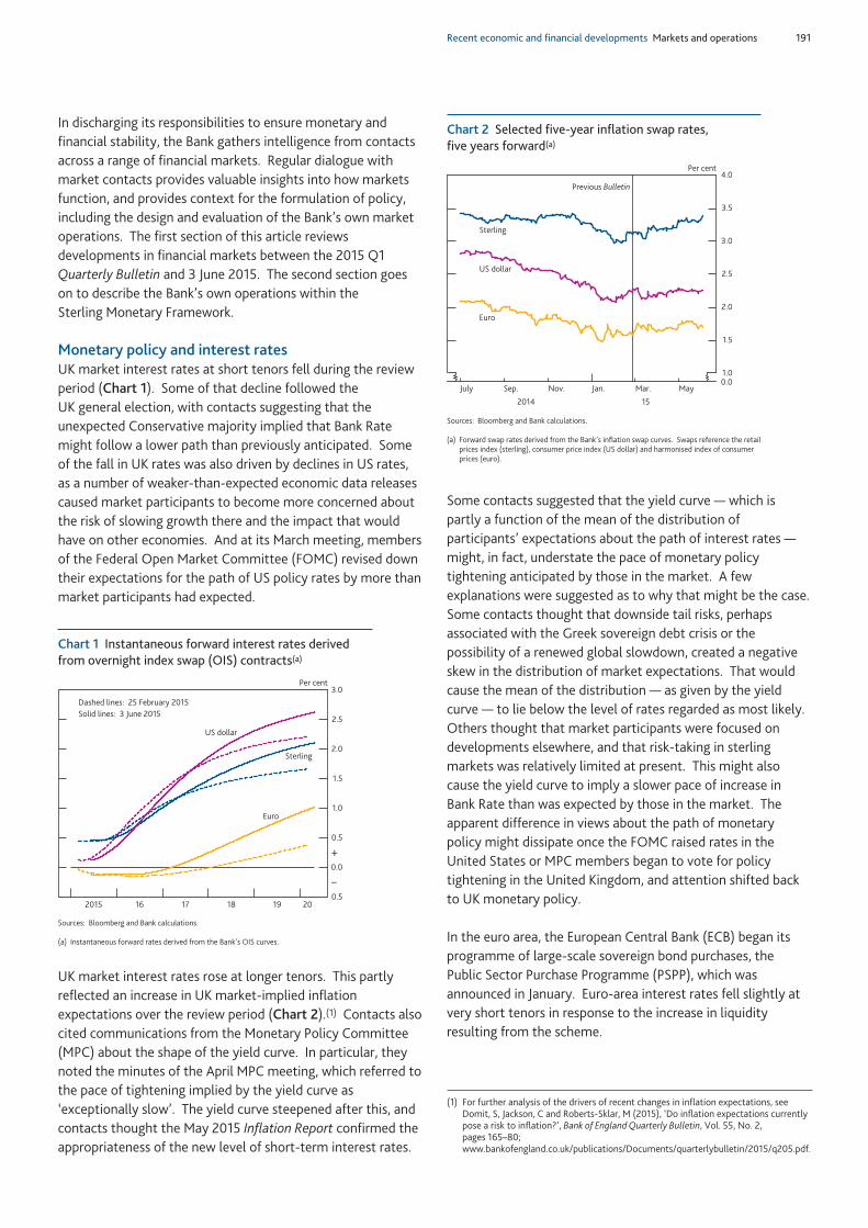
Recent economic and financial developments Markets and operations 191
In discharging its responsibilities to ensure monetary andfinancial stability, the Bank gathers intelligence from contactsacross a range of financial markets. Regular dialogue withmarket contacts provides valuable insights into how marketsfunction, and provides context for the formulation of policy,including the design and evaluation of the Bank’s own marketoperations. The first section of this article reviewsdevelopments in financial markets between the 2015 Q1Quarterly Bulletin and 3 June 2015. The second section goeson to describe the Bank’s own operations within theSterling Monetary Framework.
Monetary policy and interest ratesUK market interest rates at short tenors fell during the reviewperiod (Chart 1). Some of that decline followed theUK general election, with contacts suggesting that theunexpected Conservative majority implied that Bank Ratemight follow a lower path than previously anticipated. Someof the fall in UK rates was also driven by declines in US rates,as a number of weaker-than-expected economic data releasescaused market participants to become more concerned aboutthe risk of slowing growth there and the impact that wouldhave on other economies. And at its March meeting, membersof the Federal Open Market Committee (FOMC) revised downtheir expectations for the path of US policy rates by more thanmarket participants had expected.
UK market interest rates rose at longer tenors. This partlyreflected an increase in UK market-implied inflationexpectations over the review period (Chart 2).(1) Contacts alsocited communications from the Monetary Policy Committee(MPC) about the shape of the yield curve. In particular, theynoted the minutes of the April MPC meeting, which referred tothe pace of tightening implied by the yield curve as‘exceptionally slow’. The yield curve steepened after this, andcontacts thought the May 2015 Inflation Report confirmed theappropriateness of the new level of short-term interest rates.
Some contacts suggested that the yield curve — which ispartly a function of the mean of the distribution ofparticipants’ expectations about the path of interest rates —might, in fact, understate the pace of monetary policytightening anticipated by those in the market. A fewexplanations were suggested as to why that might be the case.Some contacts thought that downside tail risks, perhapsassociated with the Greek sovereign debt crisis or thepossibility of a renewed global slowdown, created a negativeskew in the distribution of market expectations. That wouldcause the mean of the distribution — as given by the yieldcurve — to lie below the level of rates regarded as most likely.Others thought that market participants were focused ondevelopments elsewhere, and that risk-taking in sterlingmarkets was relatively limited at present. This might alsocause the yield curve to imply a slower pace of increase inBank Rate than was expected by those in the market. Theapparent difference in views about the path of monetarypolicy might dissipate once the FOMC raised rates in theUnited States or MPC members began to vote for policytightening in the United Kingdom, and attention shifted backto UK monetary policy.
In the euro area, the European Central Bank (ECB) began itsprogramme of large-scale sovereign bond purchases, thePublic Sector Purchase Programme (PSPP), which wasannounced in January. Euro-area interest rates fell slightly atvery short tenors in response to the increase in liquidityresulting from the scheme.
+
–0.5
0.0
0.5
1.0
1.5
2.0
2.5
3.0
2015 16 17 18 19 20
Per cent
Dashed lines: 25 February 2015Solid lines: 3 June 2015
US dollar
Sterling
Euro
Sources: Bloomberg and Bank calculations.
(a) Instantaneous forward rates derived from the Bank’s OIS curves.
Chart 1 Instantaneous forward interest rates derivedfrom overnight index swap (OIS) contracts(a)
(1) For further analysis of the drivers of recent changes in inflation expectations, seeDomit, S, Jackson, C and Roberts-Sklar, M (2015), ‘Do inflation expectations currentlypose a risk to inflation?’, Bank of England Quarterly Bulletin, Vol. 55, No. 2,pages 165–80;www.bankofengland.co.uk/publications/Documents/quarterlybulletin/2015/q205.pdf.
1.0
1.5
2.0
2.5
3.0
3.5
4.0
Sterling
US dollar
Euro
July Sep. Nov. Jan. Mar. May
2014 15
Previous Bulletin
Per cent
0.0
Sources: Bloomberg and Bank calculations.
(a) Forward swap rates derived from the Bank’s inflation swap curves. Swaps reference the retailprices index (sterling), consumer price index (US dollar) and harmonised index of consumerprices (euro).
Chart 2 Selected five-year inflation swap rates,five years forward(a)
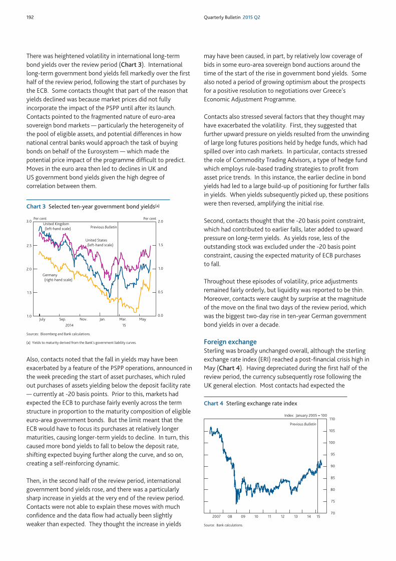
192 Quarterly Bulletin 2015 Q2
There was heightened volatility in international long-termbond yields over the review period (Chart 3). Internationallong-term government bond yields fell markedly over the firsthalf of the review period, following the start of purchases bythe ECB. Some contacts thought that part of the reason thatyields declined was because market prices did not fullyincorporate the impact of the PSPP until after its launch.Contacts pointed to the fragmented nature of euro-areasovereign bond markets — particularly the heterogeneity ofthe pool of eligible assets, and potential differences in hownational central banks would approach the task of buyingbonds on behalf of the Eurosystem — which made thepotential price impact of the programme difficult to predict.Moves in the euro area then led to declines in UK andUS government bond yields given the high degree ofcorrelation between them.
Also, contacts noted that the fall in yields may have beenexacerbated by a feature of the PSPP operations, announced inthe week preceding the start of asset purchases, which ruledout purchases of assets yielding below the deposit facility rate— currently at -20 basis points. Prior to this, markets hadexpected the ECB to purchase fairly evenly across the termstructure in proportion to the maturity composition of eligibleeuro-area government bonds. But the limit meant that theECB would have to focus its purchases at relatively longermaturities, causing longer-term yields to decline. In turn, thiscaused more bond yields to fall to below the deposit rate,shifting expected buying further along the curve, and so on,creating a self-reinforcing dynamic.
Then, in the second half of the review period, internationalgovernment bond yields rose, and there was a particularlysharp increase in yields at the very end of the review period.Contacts were not able to explain these moves with muchconfidence and the data flow had actually been slightlyweaker than expected. They thought the increase in yields
may have been caused, in part, by relatively low coverage ofbids in some euro-area sovereign bond auctions around thetime of the start of the rise in government bond yields. Somealso noted a period of growing optimism about the prospectsfor a positive resolution to negotiations over Greece’sEconomic Adjustment Programme.
Contacts also stressed several factors that they thought mayhave exacerbated the volatility. First, they suggested thatfurther upward pressure on yields resulted from the unwindingof large long futures positions held by hedge funds, which hadspilled over into cash markets. In particular, contacts stressedthe role of Commodity Trading Advisors, a type of hedge fundwhich employs rule-based trading strategies to profit fromasset price trends. In this instance, the earlier decline in bondyields had led to a large build-up of positioning for further fallsin yields. When yields subsequently picked up, these positionswere then reversed, amplifying the initial rise.
Second, contacts thought that the -20 basis point constraint,which had contributed to earlier falls, later added to upwardpressure on long-term yields. As yields rose, less of theoutstanding stock was excluded under the -20 basis pointconstraint, causing the expected maturity of ECB purchasesto fall.
Throughout these episodes of volatility, price adjustmentsremained fairly orderly, but liquidity was reported to be thin.Moreover, contacts were caught by surprise at the magnitudeof the move on the final two days of the review period, whichwas the biggest two-day rise in ten-year German governmentbond yields in over a decade.
Foreign exchangeSterling was broadly unchanged overall, although the sterlingexchange rate index (ERI) reached a post-financial crisis high inMay (Chart 4). Having depreciated during the first half of thereview period, the currency subsequently rose following theUK general election. Most contacts had expected the
Chart 3 Selected ten-year government bond yields(a)
1.0
1.5
2.0
2.5
3.0
0.0
0.5
1.0
1.5
2.0
July Sep. Nov. Jan. Mar. May
Germany (right-hand scale)
United Kingdom (left-hand scale)
United States (left-hand scale)
Per centPer cent
Previous Bulletin
2014 15
Sources: Bloomberg and Bank calculations.
(a) Yields to maturity derived from the Bank’s government liability curves.
Chart 4 Sterling exchange rate index
70
75
80
85
90
95
100
105
110
2007 08 09 10 11 12 13 14 15
Index: January 2005 = 100
Previous Bulletin
Source: Bank calculations.
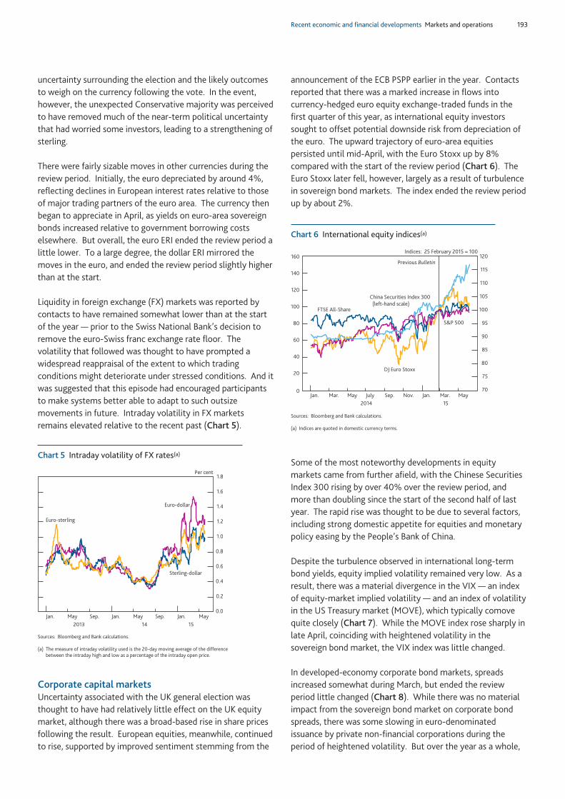
Recent economic and financial developments Markets and operations 193
uncertainty surrounding the election and the likely outcomesto weigh on the currency following the vote. In the event,however, the unexpected Conservative majority was perceivedto have removed much of the near-term political uncertaintythat had worried some investors, leading to a strengthening ofsterling.
There were fairly sizable moves in other currencies during thereview period. Initially, the euro depreciated by around 4%,reflecting declines in European interest rates relative to thoseof major trading partners of the euro area. The currency thenbegan to appreciate in April, as yields on euro-area sovereignbonds increased relative to government borrowing costselsewhere. But overall, the euro ERI ended the review period alittle lower. To a large degree, the dollar ERI mirrored themoves in the euro, and ended the review period slightly higherthan at the start.
Liquidity in foreign exchange (FX) markets was reported bycontacts to have remained somewhat lower than at the startof the year — prior to the Swiss National Bank’s decision toremove the euro-Swiss franc exchange rate floor. Thevolatility that followed was thought to have prompted awidespread reappraisal of the extent to which tradingconditions might deteriorate under stressed conditions. And itwas suggested that this episode had encouraged participantsto make systems better able to adapt to such outsizemovements in future. Intraday volatility in FX marketsremains elevated relative to the recent past (Chart 5).
Corporate capital marketsUncertainty associated with the UK general election wasthought to have had relatively little effect on the UK equitymarket, although there was a broad-based rise in share pricesfollowing the result. European equities, meanwhile, continuedto rise, supported by improved sentiment stemming from the
announcement of the ECB PSPP earlier in the year. Contactsreported that there was a marked increase in flows intocurrency-hedged euro equity exchange-traded funds in thefirst quarter of this year, as international equity investorssought to offset potential downside risk from depreciation ofthe euro. The upward trajectory of euro-area equitiespersisted until mid-April, with the Euro Stoxx up by 8%compared with the start of the review period (Chart 6). TheEuro Stoxx later fell, however, largely as a result of turbulencein sovereign bond markets. The index ended the review periodup by about 2%.
Some of the most noteworthy developments in equitymarkets came from further afield, with the Chinese SecuritiesIndex 300 rising by over 40% over the review period, andmore than doubling since the start of the second half of lastyear. The rapid rise was thought to be due to several factors,including strong domestic appetite for equities and monetarypolicy easing by the People’s Bank of China.
Despite the turbulence observed in international long-termbond yields, equity implied volatility remained very low. As aresult, there was a material divergence in the VIX — an indexof equity-market implied volatility — and an index of volatilityin the US Treasury market (MOVE), which typically comovequite closely (Chart 7). While the MOVE index rose sharply inlate April, coinciding with heightened volatility in thesovereign bond market, the VIX index was little changed.
In developed-economy corporate bond markets, spreadsincreased somewhat during March, but ended the reviewperiod little changed (Chart 8). While there was no materialimpact from the sovereign bond market on corporate bondspreads, there was some slowing in euro-denominatedissuance by private non-financial corporations during theperiod of heightened volatility. But over the year as a whole,
Chart 5 Intraday volatility of FX rates(a)
0.0
0.2
0.4
0.6
0.8
1.0
1.2
1.4
1.6
1.8
Jan. May Sep. Jan. May Sep. Jan. May
Per cent
2013 14 15
Euro-dollar
Sterling-dollar
Euro-sterling
Sources: Bloomberg and Bank calculations.
(a) The measure of intraday volatility used is the 20-day moving average of the differencebetween the intraday high and low as a percentage of the intraday open price.
Chart 6 International equity indices(a)
0
20
40
60
80
100
120
140
160
70
75
80
85
90
95
100
105
110
115
120
Jan. Mar. May July Sep. Nov. Jan. Mar. May
DJ Euro Stoxx
FTSE All-Share
S&P 500
China Securities Index 300 (left-hand scale)
2014
Previous Bulletin
Indices: 25 February 2015 = 100
15
Sources: Bloomberg and Bank calculations.
(a) Indices are quoted in domestic currency terms.
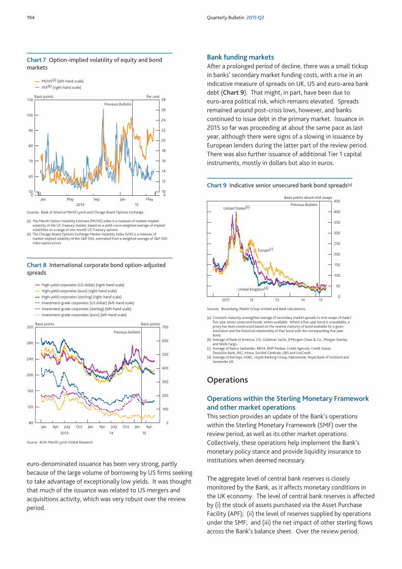
194 Quarterly Bulletin 2015 Q2
euro-denominated issuance has been very strong, partlybecause of the large volume of borrowing by US firms seekingto take advantage of exceptionally low yields. It was thoughtthat much of the issuance was related to US mergers andacquisitions activity, which was very robust over the reviewperiod.
Bank funding marketsAfter a prolonged period of decline, there was a small tickupin banks’ secondary market funding costs, with a rise in anindicative measure of spreads on UK, US and euro-area bankdebt (Chart 9). That might, in part, have been due toeuro-area political risk, which remains elevated. Spreadsremained around post-crisis lows, however, and bankscontinued to issue debt in the primary market. Issuance in2015 so far was proceeding at about the same pace as lastyear, although there were signs of a slowing in issuance byEuropean lenders during the latter part of the review period.There was also further issuance of additional Tier 1 capitalinstruments, mostly in dollars but also in euros.
Operations
Operations within the Sterling Monetary Frameworkand other market operationsThis section provides an update of the Bank’s operationswithin the Sterling Monetary Framework (SMF) over thereview period, as well as its other market operations.Collectively, these operations help implement the Bank’smonetary policy stance and provide liquidity insurance toinstitutions when deemed necessary.
The aggregate level of central bank reserves is closelymonitored by the Bank, as it affects monetary conditions inthe UK economy. The level of central bank reserves is affectedby (i) the stock of assets purchased via the Asset PurchaseFacility (APF); (ii) the level of reserves supplied by operationsunder the SMF; and (iii) the net impact of other sterling flowsacross the Bank’s balance sheet. Over the review period,
Chart 7 Option-implied volatility of equity and bondmarkets
50
60
70
80
90
100
110
10
12
14
16
18
20
22
24
26
28
Jan. May Sep. Jan. May
VIX(b) (right-hand scale)
MOVE(a) (left-hand scale)
Basis points Per cent
2014 15
Previous Bulletin
00
Sources: Bank of America Merrill Lynch and Chicago Board Options Exchange.
(a) The Merrill Option Volatility Estimate (MOVE) index is a measure of market-impliedvolatility of the US Treasury market, based on a yield-curve weighted average of impliedvolatilities on a range of one-month US Treasury options.
(b) The Chicago Board Options Exchange Market Volatility Index (VIX) is a measure ofmarket-implied volatility of the S&P 500, estimated from a weighted average of S&P 500index option prices.
Chart 8 International corporate bond option-adjustedspreads
80
120
160
200
240
280
320
0
100
200
300
400
500
600
700
Jan. Apr. July Oct. Jan. Apr. July Oct. Jan. Apr.
Basis points
High-yield corporates (US dollar) (right-hand scale)High-yield corporates (euro) (right-hand scale)High-yield corporates (sterling) (right-hand scale)Investment-grade corporates (US dollar) (left-hand scale)
Investment-grade corporates (euro) (left-hand scale)Investment-grade corporates (sterling) (left-hand scale)
Previous Bulletin
Basis points
2013 14 15
Source: BofA Merrill Lynch Global Research.
Chart 9 Indicative senior unsecured bank bond spreads(a)
Previous Bulletin
0
50
100
150
200
250
300
350
400
450
2011 12 13 14 15
Basis points above mid-swaps
United Kingdom(d)
United States(b)
Europe(c)
Sources: Bloomberg, Markit Group Limited and Bank calculations.
(a) Constant-maturity unweighted average of secondary market spreads to mid-swaps of banks’five-year senior unsecured bonds, where available. Where a five-year bond is unavailable, aproxy has been constructed based on the nearest maturity of bond available for a giveninstitution and the historical relationship of that bond with the corresponding five-yearbond.
(b) Average of Bank of America, Citi, Goldman Sachs, JPMorgan Chase & Co., Morgan Stanleyand Wells Fargo.
(c) Average of Banco Santander, BBVA, BNP Paribas, Crédit Agricole, Credit Suisse,Deutsche Bank, ING, Intesa, Société Générale, UBS and UniCredit.
(d) Average of Barclays, HSBC, Lloyds Banking Group, Nationwide, Royal Bank of Scotland andSantander UK.
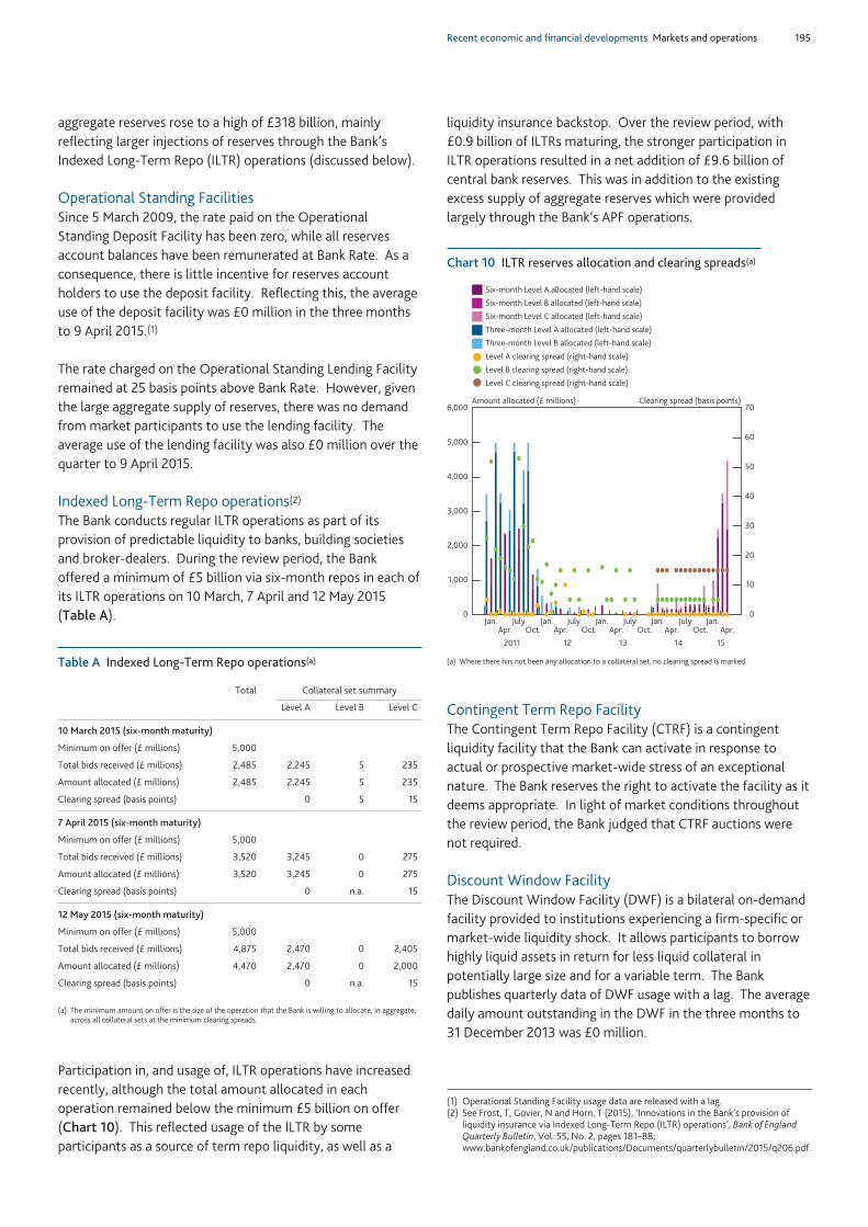
Recent economic and financial developments Markets and operations 195
aggregate reserves rose to a high of £318 billion, mainlyreflecting larger injections of reserves through the Bank’sIndexed Long-Term Repo (ILTR) operations (discussed below).
Operational Standing FacilitiesSince 5 March 2009, the rate paid on the OperationalStanding Deposit Facility has been zero, while all reservesaccount balances have been remunerated at Bank Rate. As aconsequence, there is little incentive for reserves accountholders to use the deposit facility. Reflecting this, the averageuse of the deposit facility was £0 million in the three monthsto 9 April 2015.(1)
The rate charged on the Operational Standing Lending Facilityremained at 25 basis points above Bank Rate. However, giventhe large aggregate supply of reserves, there was no demandfrom market participants to use the lending facility. Theaverage use of the lending facility was also £0 million over thequarter to 9 April 2015.
Indexed Long-Term Repo operations(2)
The Bank conducts regular ILTR operations as part of itsprovision of predictable liquidity to banks, building societiesand broker-dealers. During the review period, the Bankoffered a minimum of £5 billion via six-month repos in each ofits ILTR operations on 10 March, 7 April and 12 May 2015(Table A).
Participation in, and usage of, ILTR operations have increasedrecently, although the total amount allocated in eachoperation remained below the minimum £5 billion on offer(Chart 10). This reflected usage of the ILTR by someparticipants as a source of term repo liquidity, as well as a
liquidity insurance backstop. Over the review period, with£0.9 billion of ILTRs maturing, the stronger participation inILTR operations resulted in a net addition of £9.6 billion ofcentral bank reserves. This was in addition to the existingexcess supply of aggregate reserves which were providedlargely through the Bank’s APF operations.
Contingent Term Repo FacilityThe Contingent Term Repo Facility (CTRF) is a contingentliquidity facility that the Bank can activate in response toactual or prospective market-wide stress of an exceptionalnature. The Bank reserves the right to activate the facility as itdeems appropriate. In light of market conditions throughoutthe review period, the Bank judged that CTRF auctions werenot required.
Discount Window FacilityThe Discount Window Facility (DWF) is a bilateral on-demandfacility provided to institutions experiencing a firm-specific ormarket-wide liquidity shock. It allows participants to borrowhighly liquid assets in return for less liquid collateral inpotentially large size and for a variable term. The Bankpublishes quarterly data of DWF usage with a lag. The averagedaily amount outstanding in the DWF in the three months to31 December 2013 was £0 million.
(1) Operational Standing Facility usage data are released with a lag.(2) See Frost, T, Govier, N and Horn, T (2015), ‘Innovations in the Bank’s provision of
liquidity insurance via Indexed Long-Term Repo (ILTR) operations’, Bank of EnglandQuarterly Bulletin, Vol. 55, No. 2, pages 181–88;www.bankofengland.co.uk/publications/Documents/quarterlybulletin/2015/q206.pdf.
Table A Indexed Long-Term Repo operations(a)
Total Collateral set summary
Level A Level B Level C
10 March 2015 (six-month maturity)
Minimum on offer (£ millions) 5,000
Total bids received (£ millions) 2,485 2,245 5 235
Amount allocated (£ millions) 2,485 2,245 5 235
Clearing spread (basis points) 0 5 15
7 April 2015 (six-month maturity)
Minimum on offer (£ millions) 5,000
Total bids received (£ millions) 3,520 3,245 0 275
Amount allocated (£ millions) 3,520 3,245 0 275
Clearing spread (basis points) 0 n.a. 15
12 May 2015 (six-month maturity)
Minimum on offer (£ millions) 5,000
Total bids received (£ millions) 4,875 2,470 0 2,405
Amount allocated (£ millions) 4,470 2,470 0 2,000
Clearing spread (basis points) 0 n.a. 15
(a) The minimum amount on offer is the size of the operation that the Bank is willing to allocate, in aggregate,across all collateral sets at the minimum clearing spreads.
Chart 10 ILTR reserves allocation and clearing spreads(a)
Jan.Apr.
JulyOct.
Jan.Apr.
JulyOct.
Jan.Apr.
Three-month Level A allocated (left-hand scale)
Three-month Level B allocated (left-hand scale)
Six-month Level A allocated (left-hand scale)
Six-month Level B allocated (left-hand scale)
Six-month Level C allocated (left-hand scale)
Level A clearing spread (right-hand scale)
Level B clearing spread (right-hand scale)
Level C clearing spread (right-hand scale)
Amount allocated (£ millions) Clearing spread (basis points)
0
1,000
2,000
3,000
4,000
5,000
6,000
0
10
20
30
40
50
60
70
2011 12 13 14 15
JulyOct.
Jan.Apr.
JulyOct.
Jan.Apr.
(a) Where there has not been any allocation to a collateral set, no clearing spread is marked.
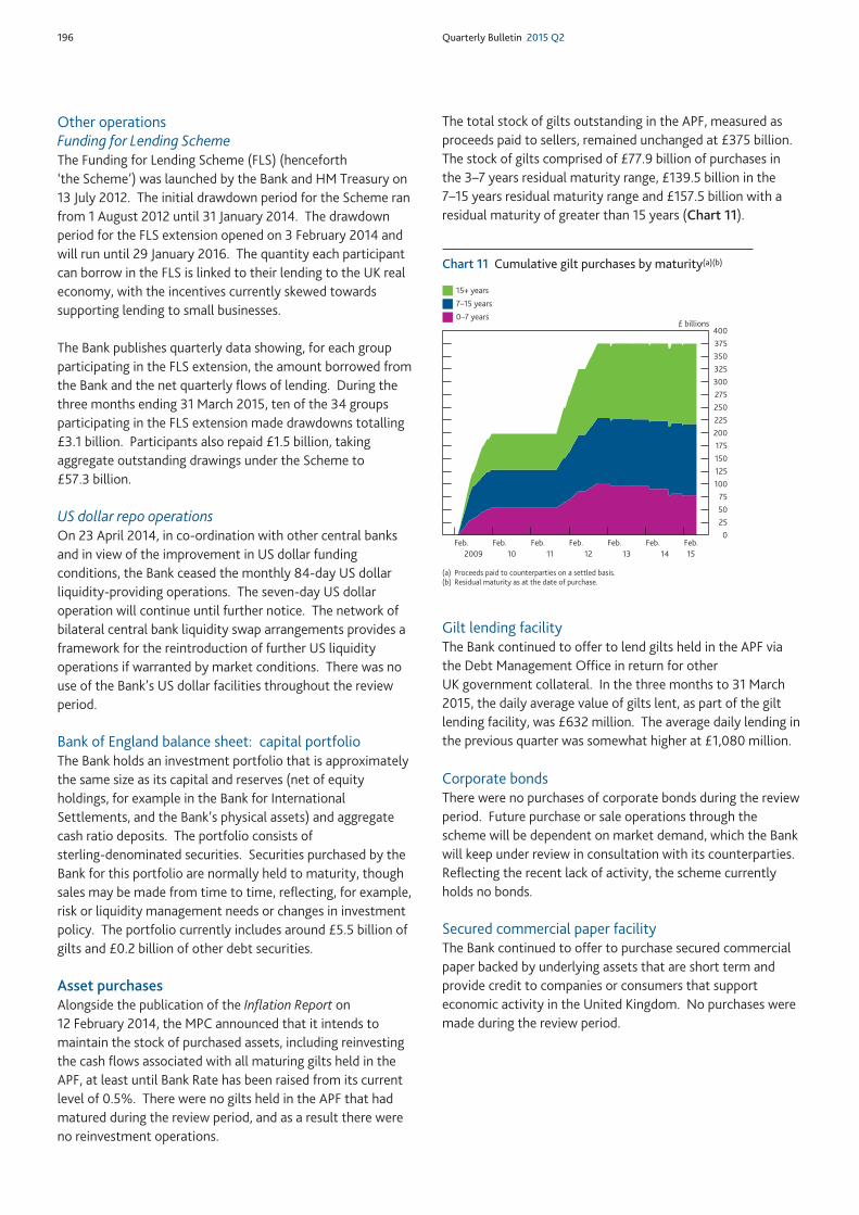
196 Quarterly Bulletin 2015 Q2
Other operationsFunding for Lending SchemeThe Funding for Lending Scheme (FLS) (henceforth‘the Scheme’) was launched by the Bank and HM Treasury on13 July 2012. The initial drawdown period for the Scheme ranfrom 1 August 2012 until 31 January 2014. The drawdownperiod for the FLS extension opened on 3 February 2014 andwill run until 29 January 2016. The quantity each participantcan borrow in the FLS is linked to their lending to the UK realeconomy, with the incentives currently skewed towardssupporting lending to small businesses.
The Bank publishes quarterly data showing, for each groupparticipating in the FLS extension, the amount borrowed fromthe Bank and the net quarterly flows of lending. During thethree months ending 31 March 2015, ten of the 34 groupsparticipating in the FLS extension made drawdowns totalling£3.1 billion. Participants also repaid £1.5 billion, takingaggregate outstanding drawings under the Scheme to£57.3 billion.
US dollar repo operationsOn 23 April 2014, in co-ordination with other central banksand in view of the improvement in US dollar fundingconditions, the Bank ceased the monthly 84-day US dollarliquidity-providing operations. The seven-day US dollaroperation will continue until further notice. The network ofbilateral central bank liquidity swap arrangements provides aframework for the reintroduction of further US liquidityoperations if warranted by market conditions. There was nouse of the Bank’s US dollar facilities throughout the reviewperiod.
Bank of England balance sheet: capital portfolioThe Bank holds an investment portfolio that is approximatelythe same size as its capital and reserves (net of equityholdings, for example in the Bank for InternationalSettlements, and the Bank’s physical assets) and aggregatecash ratio deposits. The portfolio consists ofsterling-denominated securities. Securities purchased by theBank for this portfolio are normally held to maturity, thoughsales may be made from time to time, reflecting, for example,risk or liquidity management needs or changes in investmentpolicy. The portfolio currently includes around £5.5 billion ofgilts and £0.2 billion of other debt securities.
Asset purchasesAlongside the publication of the Inflation Report on12 February 2014, the MPC announced that it intends tomaintain the stock of purchased assets, including reinvestingthe cash flows associated with all maturing gilts held in theAPF, at least until Bank Rate has been raised from its currentlevel of 0.5%. There were no gilts held in the APF that hadmatured during the review period, and as a result there wereno reinvestment operations.
The total stock of gilts outstanding in the APF, measured asproceeds paid to sellers, remained unchanged at £375 billion.The stock of gilts comprised of £77.9 billion of purchases inthe 3–7 years residual maturity range, £139.5 billion in the7–15 years residual maturity range and £157.5 billion with aresidual maturity of greater than 15 years (Chart 11).
Gilt lending facilityThe Bank continued to offer to lend gilts held in the APF viathe Debt Management Office in return for otherUK government collateral. In the three months to 31 March2015, the daily average value of gilts lent, as part of the giltlending facility, was £632 million. The average daily lending inthe previous quarter was somewhat higher at £1,080 million.
Corporate bondsThere were no purchases of corporate bonds during the reviewperiod. Future purchase or sale operations through thescheme will be dependent on market demand, which the Bankwill keep under review in consultation with its counterparties.Reflecting the recent lack of activity, the scheme currentlyholds no bonds.
Secured commercial paper facilityThe Bank continued to offer to purchase secured commercialpaper backed by underlying assets that are short term andprovide credit to companies or consumers that supporteconomic activity in the United Kingdom. No purchases weremade during the review period.
Chart 11 Cumulative gilt purchases by maturity(a)(b)
0255075
100125150175200225250275300325350375400
Feb. Feb. Feb. Feb. Feb. Feb. Feb.
15+ years
7–15 years
0–7 years£ billions
14131211102009 15
(a) Proceeds paid to counterparties on a settled basis.(b) Residual maturity as at the date of purchase.

Report
Quarterly Bulletin Report 197
198 Quarterly Bulletin 2015 Q2
Introduction
The London Foreign Exchange Joint Standing Committee(FXJSC — hereon, ‘the Committee’) was established in 1973,under the auspices of the Bank of England, as a forum forbanks and brokers to discuss broad market issues. TheCommittee comprises senior staff from many of the majorbanks operating in the wholesale foreign exchange (FX)market in London, representatives from brokers, tradeassociations including the Wholesale Markets Brokers’Association (WMBA), the Association of Corporate Treasurers(ACT) — representing corporate users of the FX market, theInvestment Association — representing UK investmentmanagers and the British Bankers’ Association (BBA). TheFinancial Conduct Authority (FCA) is also a member. A list ofthe members of the Committee as at end-2014 can befound at the end of this article. The Committee metsix times during 2014.
The Committee continued to focus on the main issuesimpacting the functioning of, and liquidity within, theFX market. The key items of discussion during 2014 were theFair and Effective Markets Review(1) (FEMR), and the FinancialStability Board’s (FSB’s) FX Benchmark consultation andrecommendations. The Committee continued to assess theimpact of both EU and international regulatory reforms onFX markets. The Committee also discussed drivers ofFX volatility during 2014, such as developments in emergingmarkets, the Scottish referendum and the implications ofsanctions on Russia on over-the-counter (OTC) transactions.
The Committee received presentations from a number ofguest speakers during the year. The Global Financial MarketsAssociation’s Global FX Division summarised the quantitativestudy they undertook on the OTC FX options market. A guestspeaker from Bluecrest Capital provided an overview of theirresearch into FX market liquidity trends. In addition the FCAgave a presentation on the revised Markets in FinancialInstruments Directive and Regulation (MiFID2), while a guestspeaker from Kingfisher plc provided a view of FX marketsfrom a corporate perspective.
Non-Investment Products (NIPs) Code
The NIPs Code is a voluntary code of good market practicedrawn up by market practitioners covering the FX market inthe United Kingdom as well as the markets for wholesalebullion and wholesale deposits. The Code is published by theFXJSC, with contributions from the FXJSC Operations andLegal subgroups, the Sterling Money Markets Liaison Groupand the Management Committee of the London BullionMarket Association for the relevant sections. The currentversion of the Code was published in November 2011.(2)
The FXJSC was one of eight FX committees in major financialcentres to endorse the ‘Global Preamble Codes of best marketpractice and shared global principles’,(3) which was finalised atthe annual meeting of the global FX committees in Tokyo,Japan in March 2015. The Preamble seeks to providehigh-level globally harmonised guidance and covers topicssuch as personal conduct, confidentiality and market conduct,and policies for execution practices reflecting a number of theFSB’s FX Benchmark recommendations.
The FXJSC is also awaiting the recommendations of FEMR andthe finalisation of the subordinate legislation for the EuropeanMarket Infrastructure Regulation (EMIR) and MiFID2 beforeconsidering publishing an update to the NIPs Code.
Work of the FXJSC operations subgroup
The operations subgroup was established in 2002. Itsmembers are operations managers from many major banksactive in the London wholesale FX market, as well asrepresentatives from service providers and trade associationsand also from the FCA. The group met six times in 2014.
This article reviews the work undertaken by the London Foreign Exchange Joint StandingCommittee during 2014.
A review of the work of the London Foreign Exchange Joint Standing Committee in 2014
(1) More information on the Fair and Effective Markets Review can be found at:www.bankofengland.co.uk/markets/Pages/fmreview.aspx.
(2) The NIPs Code can be accessed at: www.bankofengland.co.uk/markets/Documents/forex/fxjsc/nipscode1111.pdf.
(3) The Global Preamble can be accessed at: www.bankofengland.co.uk/markets/Documents/forex/fxjsc/globalpreamble.pdf.
Report The London Foreign Exchange Joint Standing Committee 199
During the year, the subgroup continued to discuss themesimpacting FX market operations, including developments infinancial regulations and technology. The subgroup receivedpresentations on MiFID2, and cyber security definitions andbest practice. CLS provided a summary of their FX settlementsurvey results and SWIFT introduced FX trade volume analysisthey had undertaken using their messaging data. Theoperations subgroup work plan for 2014 included topics suchas analysing synergies between FX turnover surveys, exploringways to improve EU trade reporting, and looking at ways toimprove post-trade risk management processes. On the lattertwo working groups, the subgroup agreed to contribute theirfinal findings and analysis completed in 2014 to otherinternational forums following similar issues, such as theGlobal Financial Markets Association.
Work of the FXJSC legal subgroup
The legal subgroup was established in 2004 and comprisesfifteen professionals providing in-house legal counsel for manyof the major institutions involved in the wholesale FX marketin London. The group met three times in 2014.
It continued to make an important contribution through itsprovision of legal support to the work of the FXJSC mainCommittee and its subgroups. During 2014, the legalsubgroup welcomed guest speakers from the InternationalSwaps and Derivatives Association and Allen & Overy onUkraine and Russian sanctions, as well as speakers frommember firms to discuss how regulatory change affects theFX market. The group also discussed developments in theglobal FX market including the ongoing FEMR work.
The legal subgroup continued to liaise with a range of otherforeign legal committees to keep abreast of developments inFX markets.
Work of the FXJSC buy-side subgroup
The buy-side subgroup met four times in 2014, following thesubgroup’s reconstitution in November 2013. The subgroupmembership includes representatives from the buy-sideinstitutions active in wholesale FX markets.
The subgroup discussed changes in market conditions,including FX market liquidity in domestic and emergingmarkets. Initiatives such as the FSB FX Benchmarkconsultation and FEMR were also discussed. The subgroupcontinued to consider the impact of a changing regulatoryenvironment on market conditions, including theimplementation of the EMIR.
Work of the FXJSC chief dealers’ subgroup
The chief dealers’ subgroup was established in July 2005. Thesubgroup did not meet in 2014 and has formally beendisbanded.
International co-operation
Liaison between the eight FX committees based in differentinternational financial centres (London, Frankfurt for theeuro area, Hong Kong, New York, Tokyo, Singapore, Sydneyand Toronto) continued during the year. In April 2014, theAustralian Foreign Exchange Committee hosted an annualglobal meeting of the FX committees.(1) Topics discussedincluded assessing changes in market structure and theevolving execution landscape, the FSB’s FX Benchmark work,FX industry codes of conduct and international regulatoryreform initiatives such as new EU trade reporting requirementsfor derivatives and US Swap Execution Facility regulations.
International survey results overview
Thirty banks representing the most active participants in theUK FX market contributed to the 20th and 21st FXJSCsemi-annual surveys of UK FX turnover in April andOctober 2014. Total UK turnover rose 19% in the year toOctober 2014, 11% higher than in April 2014. This is thehighest level of turnover since survey inception and 5% higherthan previous highs recorded in April 2013 (Chart 1).
This trend was broadly consistent with other global centres:total turnover across the six reporting centres rose 21%year-on-year in October 2014. In particular, Singaporeregistered the largest relative increase in turnover (up 40%),followed by the United States (up 34%), Canada (up 20%) andUnited Kingdom (up 19%). In contrast, turnover in Australiafell 11% and turnover in Tokyo was stable.
Average daily turnover in the majority of FX productsincreased in October 2014 (Chart 2). Average daily spotturnover in the United Kingdom rose to US$1,110 billion inOctober 2014, 44% higher than the previous year. This wasconsistent with a broad global increase in spot activity,including in the United States (up 48%). Conversely, FX swapturnover fell back in October 2014, to April 2013 levels,following a temporary increase to survey highs in April 2014.
The proportion of FX trades with ‘other financial institutions’(OFIs), including hedge funds, non-reporting banks, centralbanks and sovereign wealth funds continued to rise. Thisincrease was particularly prominent in FX spot markets, where
(1) Full minutes of the 2014 meeting can be found here: www.rba.gov.au/afxc/meetings/gfxc/2014/gfxc-minutes-20140411.html.
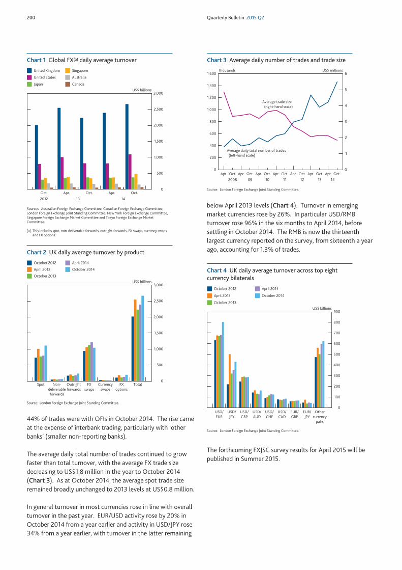
200 Quarterly Bulletin 2015 Q2
44% of trades were with OFIs in October 2014. The rise cameat the expense of interbank trading, particularly with ‘otherbanks’ (smaller non-reporting banks).
The average daily total number of trades continued to growfaster than total turnover, with the average FX trade sizedecreasing to US$1.8 million in the year to October 2014(Chart 3). As at October 2014, the average spot trade sizeremained broadly unchanged to 2013 levels at US$0.8 million.
In general turnover in most currencies rose in line with overallturnover in the past year. EUR/USD activity rose by 20% inOctober 2014 from a year earlier and activity in USD/JPY rose34% from a year earlier, with turnover in the latter remaining
below April 2013 levels (Chart 4). Turnover in emergingmarket currencies rose by 26%. In particular USD/RMBturnover rose 96% in the six months to April 2014, beforesettling in October 2014. The RMB is now the thirteenthlargest currency reported on the survey, from sixteenth a yearago, accounting for 1.3% of trades.
The forthcoming FXJSC survey results for April 2015 will bepublished in Summer 2015.
0
500
1,000
1,500
2,000
2,500
3,000
Oct. Apr. Oct. Apr. Oct.
United Kingdom Singapore
United States Australia
Japan CanadaUS$ billions
2012 13 14
Sources: Australian Foreign Exchange Committee, Canadian Foreign Exchange Committee,London Foreign Exchange Joint Standing Committee, New York Foreign Exchange Committee,Singapore Foreign Exchange Market Committee and Tokyo Foreign Exchange MarketCommittee.
(a) This includes spot, non-deliverable forwards, outright forwards, FX swaps, currency swapsand FX options.
Chart 1 Global FX(a) daily average turnover
0
1
2
3
4
5
6
0
200
400
600
800
1,000
1,200
1,400
1,600
Apr. Oct. Apr. Oct. Apr. Oct. Apr. Oct. Apr. Oct. Apr. Oct. Apr. Oct.
Average daily total number of trades (left-hand scale)
Average trade size (right-hand scale)
US$ millionsThousands
2008 11 121009 13 14
Source: London Foreign Exchange Joint Standing Committee.
Chart 3 Average daily number of trades and trade size
0
500
1,000
1,500
2,000
2,500
3,000
Spot Non-deliverableforwards
Outrightforwards
FXswaps
Currencyswaps
FXoptions
Total
US$ billionsOctober 2013
October 2012 April 2014
April 2013 October 2014
Source: London Foreign Exchange Joint Standing Committee.
Chart 2 UK daily average turnover by product
0
100
200
300
400
500
600
700
800
900
USD/EUR
USD/JPY
USD/GBP
USD/AUD
USD/CHF
USD/CAD
EUR/GBP
EUR/JPY
Othercurrency
pairs
US$ billionsOctober 2013
October 2012 April 2014
April 2013 October 2014
Source: London Foreign Exchange Joint Standing Committee.
Chart 4 UK daily average turnover across top eightcurrency bilaterals

Report The London Foreign Exchange Joint Standing Committee 201
Members of the London Foreign Exchange Joint Standing mainCommittee as at December 2014
Name Firm/organisation
Brian Welch Association of Corporate Treasurers
Christopher Bae Bank of America Merrill Lynch
Rob Loewy Bank of China
Richard Gill Bank of New York Mellon
Fujio Nishio Bank of Tokyo-Mitsubishi
Adrian McGowan Barclays
Eric Auld BNP Paribas
Andrew Rogan British Bankers’ Association
James Bindler Citigroup
David Puth CLS
Gil Mandelzis EBS BrokerTec
Heather Pilley Financial Conduct Authority
Tom Springbett Financial Conduct Authority
Frederic Boillereau HSBC
Troy Rohrbaugh JPMorgan Chase
Tim Carrington Royal Bank of Scotland
Richard Metcalfe The Investment Association
Phil Weisberg Thomson Reuters
James Potter Tullett Prebon
George Athanasopoulos UBS
Alex McDonald Wholesale Markets Brokers’ Association
Chris Allen Barclays, Chair, legal subgroup
Jacqueline Joyston-Bechal Bank of England, Secretariat, legal subgroup
Graeme Munro JPMorgan Chase, Chair, operations subgroup
Lisa Scott-Smith Millennium Global, Chair, FX buy-side subgroup
Michael Cross (Chair) Bank of England
Robert Spillett and Joanna West(Secretariat) Bank of England
Tables of membership at end-2014
Members of the London Foreign Exchange Joint StandingCommittee operations subgroup as at December 2014
Name Firm/organisation
Nigel Brigden Association of Foreign Banks
Sarah Mullen Bank of America Merrill Lynch
Louise Lee Bank of England
Pamela Bald Bank of New York Mellon
Duncan Lord Barclays
Andrew Rogan British Bankers’ Association
Leigh Meyer Citigroup
John Hagon CLS Services
Damian Brettkelly Deutsche Bank
Kasia Abendan Financial Conduct Authority
John Blythe Goldman Sachs
Trevor Evans HSBC
Graeme Munro (Chair) JPMorgan Chase
Stephen Nankivell Nomura
Isabelle Dennigan RBC
Richard Norman Royal Bank of Scotland
Ian Cowell State Street
Joe Halberstadt SWIFT
Nancy Riyad UBS
Jacqueline Joyston-Bechal Bank of England, Secretariat, legal subgroup
Robert Spillett, Joanna West andChristopher Hood (Secretariat) Bank of England
Members of the London Foreign Exchange Joint StandingCommittee legal subgroup as at December 2014
Name Firm/organisation
Jateen Shah Bank of America Merrill Lynch
Alan Brewer Barclays
Richard Haynes/Sharon Blackman Citigroup
Gaynor Wood CLS Services
Simon Goldsworthy/Charlotte Hannavy Deutsche Bank
David Harris Financial Conduct Authority
Dan Parker Goldman Sachs
Christian Bettley HSBC
Emma Rickett JPMorgan Chase
Barra Little Morgan Stanley
Joanna Wormell Royal Bank of Scotland
Alistair Cleverly/Kate Binions Standard Chartered
Richard Lamb/Sergey Likhosherstov UBS
Chris Allen (Chair) Barclays
Jacqueline Joyston-Bechal (Secretariat) Bank of England
Members of the London Foreign Exchange Joint StandingCommittee buy-side subgroup as at December 2014
Name Firm/organisation
Murray Steel AHL
Alexis Blair Aspect Capital
Lee Sanders AXA
Jatin Vara BlackRock
Marcus Browning Bluecrest Capital
David Bowen Goldman Sachs
Richard Purssell Insight
Lisa Scott-Smith (Chair) Millennium Global
Jonathan Griggs Rogge
Aadarsh Malde Tudor
John Dacosta Wellington
Michael Cross Bank of England
Robert Spillett (Secretariat) Bank of England
Jacqueline Joyston-Bechal Bank of England, Secretariat, legal subgroup


Summaries ofworking papers
Quarterly Bulletin Working papers 203

204 Quarterly Bulletin 2015 Q2
In recent years dynamic stochastic general equilibrium (DSGE)models have emerged as important tools for forecasting andpolicy analysis, thanks to their attractive theoretical featuresand their improved forecasting ability. These models arebased on clear theoretical principles that explain how theeconomy as a whole interacts and evolves over time (hence‘dynamic’) in the presence of random (‘stochastic’) shocks. Asthey become more widely used in policy applications,diagnosing their fit to the observed data becomes crucial.
The recent crisis has brought new relevance to this question;key causes of the crisis and its protraction, such as the housingmarket, financial markets, the labour market and the fiscalsector, are often very stylised or missing in most policy macro-models. In some cases this may be rightly so, if themodel can represent the data well without them. But ifinstead the model misses some crucial aspects of theeconomy’s dynamics, then we must expand the model toinclude those features. We therefore need tools to assesswhich of these channels and transmission mechanisms arerelevant at various points in the conjuncture. This paper aimsto make progress in this direction.
The proposal is to exploit a data-rich environment and focuson the interaction between a large number of macroeconomicvariables and the model to capture the likely sources andmagnitude of the model misspecification. If a model is well specified, then it should represent the data well and
off-model variables should not help predict the driving forces of the model, which are generally assumed to evolve inan exogenous fashion. Finding that variables that are notexplicitly in the model can help predict the model’s dynamicsis then an indication that some channels are missing. Forecast error variance decompositions, which indicate howmuch of the overall dynamics of the model’s variables isdriven by external off-model information, can help assess how large the misspecification is. By looking at whichvariables help predict the driving processes of the model, wecan also gather information about which specific channels aremissing.
The paper puts the proposed methodology to two tests. First,a ‘Monte Carlo’ experiment is undertaken in which theapproach is explored using artificial data sets generated withrandom variations from a known model. Second, it is appliedto US data up to 2011 using a widely used benchmark DSGEmodel. It emerges that, despite the richness of model’sstructure, the auxiliary off-model information can account fora sizable portion of the forecast error variance decompositionof its driving processes. The investment shock, which affectsthe transformation of consumption goods to installed capital,appears to be the most misspecified. It is possible to confirmthe conjecture that the investment-specific shock picks upunmodelled aspects of the financial markets and can be seenas a proxy for overall health of the financial system byextending the model to include financial frictions.
Can a data-rich environment help identify the sources of modelmisspecification?
Summary of Working Paper No. 527 Francesca Monti
Quarterly Bulletin Working papers 205
Modern macroeconomics incorporates the notion that thefundamental drivers of the business cycle are random ‘shocks’,which are then disseminated around the economy in waysdescribed by our models. Often, the occurrence of thoseshocks is assumed to be governed by Gaussian (or Normal)distributions. But this may be unrealistic.
Could empirical macroeconomic models with otherdistributions of shocks be able to better predict economicdownturns? Specifically, since the onset of the Great Recession and during the ensuing uncertaintysurrounding the political and economic environment, bothacademic and policy circles have paid increasing attention toextreme events. Many argue that recent events could hardlybe explained or predicted by models that are based on aGaussian shock structure, mainly because these models assignvirtually zero probability to the macroeconomic outcomesthat we have recently observed.
To address this criticism, the present paper develops a vectorautoregressive model (VAR) — statistical models consisting ofa system of dynamic linear regressions explaining a set ofvariables where the explanatory variables are in each case lagsof the whole set — which is aimed at providing a moreaccurate modelling of uncertainty. We aim to achieve this byadding two features to the standard VAR.
First, we explicitly account for extreme events by replacing theassumption that the statistical residuals follow a Normaldistribution with the assumption that they follow a Student’st distribution. A key property of Student’s t distribution is thatit assigns more probability mass to extreme events, such asthe meltdown of the financial system in 2008. Second, ourmodel also accounts for the fact that the economy may face apersistently high-volatility environment (such as the late1970s) followed by a relatively long period of low-volatilityenvironment (such as the 1990s).
To test whether our model can forecast more accuratelyrelative to more standard benchmark models, we use monthlydata on industrial production growth, the inflation rate, theshort-term interest rate and the S&P 500 return for theUnited States. The estimation results suggest that bothmodelling features provide increased forecast accuracy. Thefat tails assumption appears especially important over theGreat Recession. With benchmark VARs (using Normaldistributions) there was essentially no chance of observing theactual collapse of US industrial production (equal to -4.3%)observed in September 2008. According to our model, thisoutcome was much more likely to happen. Moreover, weprovide further evidence on a set of countries, which confirmsthe importance of providing a more realistic modelling ofuncertainty when making statistical forecasts.
Forecasting with VAR models: fat tails and stochastic volatility
Summary of Working Paper No. 528 Ching-Wai (Jeremy) Chiu, Haroon Mumtaz and Gabor Pinter
206 Quarterly Bulletin 2015 Q2
Since the Great Recession, banks have increasingly beenincorporated into macroeconomic models. However, thisliterature confronts many unresolved issues. This paper showsthat many of them are attributable to the use of theintermediation of loanable funds (ILF) model of banking. In theILF model, bank loans represent the intermediation of realsavings, or loanable funds, between non-bank savers and non-bank borrowers. But in the real world, the key function ofbanks is the provision of financing, or the creation of newmonetary purchasing power through loans, for a single agentthat is both borrower and depositor. The bank therefore createsits own funding, deposits, in the act of lending, in a transactionthat involves no intermediation whatsoever. Third parties areonly involved in that the borrower/depositor needs to be surethat others will accept his new deposit in payment for goods,services or assets. This is never in question, because bankdeposits are any modern economy’s dominant medium ofexchange.
Furthermore, if the loan is for physical investment purposes,this new lending and money is what triggers investment andtherefore, by the national accounts identity of saving andinvestment (for closed economies), saving. Saving is therefore aconsequence, not a cause, of such lending. Saving does notfinance investment, financing does. To argue otherwiseconfuses the respective macroeconomic roles of resources(saving) and debt-based money (financing).
The paper shows that this financing through money creation(FMC) description of the role of banks can be found in manypublications of the world’s leading central banks. What hasbeen much more challenging is the incorporation of the FMCview’s insights into dynamic stochastic general equilibrium(DSGE) models that can be used to study the role of banks in macroeconomic cycles. DSGE models are the workhorse of modern macroeconomics, and are a key tool in macroprudential policy analysis. They study the interactions ofmultiple economic agents that optimise their utility or profitobjectives over time, subject to budget constraints and randomshocks.
The key contribution of this paper is therefore the developmentof the essential ingredients of DSGE models with FMC banks,and a comparison of their predictions with those of otherwiseidentical DSGE models with ILF banks. The result of our modelcomparison exercise is that, compared to ILF models, andfollowing identical shocks to financial conditions that affect the
creditworthiness of bank borrowers, FMC models predictchanges in the size of bank balance sheets that are far larger,happen much faster, and have much greater effects on the realeconomy, while the adjustment process depends far less onchanges in lending spreads, the dominant adjustment channelin ILF models. Compared to ILF models, FMC models alsopredict procyclical rather than countercyclical bank leverage,and a significant role for quantity rationing of credit rather thanprice rationing during downturns. We show that thesepredictions of FMC models are much more in line with thestylised facts than those of ILF models.
The fundamental reason for these differences is that savings inthe ILF model of banking need to be accumulated through aprocess of either producing additional goods or foregoingconsumption of existing goods, a physical process that by itsvery nature is slow and continuous. On the other hand, FMCbanks that create purchasing power can technically do soinstantaneously and discontinuously, because the process doesnot involve physical goods, but rather the creation of moneythrough the simultaneous expansion of both sides of banks’balance sheets. While money is essential to facilitatingpurchases and sales of real resources outside the bankingsystem, it is not itself a physical resource, and can be created atnear zero cost. In other words, the ILF model is fundamentally amodel of banks as barter institutions, while the FMC model isfundamentally a model of banks as monetary institutions.
The fact that banks technically face no limits to increasing thestocks of loans and deposits instantaneously anddiscontinuously does not, of course, mean that they do not faceother limits to doing so. But the most important limit,especially during the boom periods of financial cycles when allbanks simultaneously decide to lend more, is their ownassessment of the implications of new lending for theirprofitability and solvency, rather than external constraints suchas loanable funds, or the availability of central bank reserves.
This finally takes us to the venerable deposit multiplier (DM)model of banking, which suggests that the availability of centralbank high-powered money imposes another limit to rapidchanges in the size of bank balance sheets. The DM modelhowever does not recognise that modern central banks targetinterest rates, and are committed to supplying as many reserves(and cash) as banks demand at that rate. The quantity ofreserves is therefore a consequence, not a cause, of lending andmoney creation.
Banks are not intermediaries of loanable funds — and why thismatters
Summary of Working Paper No. 529 Zoltan Jakab and Michael Kumhof

Quarterly Bulletin Appendices 207
Appendices
208 Quarterly Bulletin 2015 Q2
The articles that have been published recently in theQuarterly Bulletin are listed below. Articles fromDecember 1960 to Winter 2004 are available on theBank’s website at:
www.bankofengland.co.uk/archive/Pages/digitalcontent/historicpubs/quarterlybulletins.aspx.
Articles from Spring 2005 onwards are available at:
www.bankofengland.co.uk/publications/Pages/quarterlybulletin/default.aspx.
Articles
2011 Q3– The United Kingdom’s quantitative easing policy: design, operation and impact– Bank resolution and safeguarding the creditors left behind– Developments in the global securities lending market– Measuring financial sector output and its contribution to UK GDP– The Money Market Liaison Group Sterling Money Market Survey– Monetary Policy Roundtable
2011 Q4– Understanding recent developments in UK external trade– The financial position of British households: evidence from the 2011 NMG Consulting survey– Going public: UK companies’ use of capital markets– Trading models and liquidity provision in OTC derivatives markets
2012 Q1– What might be driving the need to rebalance in the United Kingdom?– Agents’ Special Surveys since the start of the financial crisis– What can the oil futures curve tell us about the outlook for oil prices?– Quantitative easing and other unconventional monetary policies: Bank of England conference summary– The Bank of England’s Special Liquidity Scheme– Monetary Policy Roundtable
2012 Q2– How has the risk to inflation from inflation expectations evolved?– Public attitudes to monetary policy and satisfaction with the Bank– Using changes in auction maturity sectors to help identify the impact of QE on gilt yields
– UK labour productivity since the onset of the crisis — an international and historical perspective– Considering the continuity of payments for customers in a bank’s recovery or resolution– A review of the work of the London Foreign Exchange Joint Standing Committee in 2011
2012 Q3– RAMSI: a top-down stress-testing model developed at the Bank of England– What accounts for the fall in UK ten-year government bond yields?– Option-implied probability distributions for future inflation– The Bank of England’s Real-Time Gross Settlement infrastructure– The distributional effects of asset purchases– Monetary Policy Roundtable
2012 Q4– The Funding for Lending Scheme– What can the money data tell us about the impact of QE?– Influences on household spending: evidence from the 2012 NMG Consulting survey– The role of designated market makers in the new trading landscape– The Prudential Regulation Authority
2013 Q1– Changes to the Bank of England– The profile of cash transfers between the Asset Purchase Facility and Her Majesty’s Treasury– Private equity and financial stability– Commercial property and financial stability– The Agents’ company visit scores– The Bank of England Bank Liabilities Survey– Monetary Policy Roundtable
2013 Q2– Macroeconomic uncertainty: what is it, how can we measure it and why does it matter?– Do inflation expectations currently pose a risk to the economy? – Public attitudes to monetary policy– Cross-border bank credit and global financial stability– The Old Lady of Threadneedle Street– Central counterparties: what are they, why do they matter and how does the Bank supervise them?– A review of the work of the London Foreign Exchange Joint Standing Committee in 2012
Contents of recent Quarterly Bulletins
Quarterly Bulletin Appendices 209
2013 Q3– Macroprudential policy at the Bank of England– Bank capital and liquidity– The rationale for the prudential regulation and supervision of insurers– Recent developments in the sterling overnight money market– Nowcasting world GDP and trade using global indicators– The Natural Rate Hypothesis: an idea past its sell-by date– Monetary Policy Roundtable
2013 Q4– SME forbearance and its implications for monetary and financial stability– Bringing down the Great Wall? Global implications of capital account liberalisation in China– Banknotes, local currencies and central bank objectives– Banks’ disclosure and financial stability– Understanding the MPC’s forecast performance since mid-2010– The financial position of British households: evidence from the 2013 NMG Consulting survey– What can company data tell us about financing and investment decisions?– Tiering in CHAPS– The foreign exchange and over-the-counter interest rate derivatives market in the United Kingdom– Qualitative easing: a new tool for the stabilisation of financial markets
2014 Q1– Money in the modern economy: an introduction– Money creation in the modern economy– The Court of the Bank of England– Dealing with a banking crisis: what lessons can be learned from Japan’s experience?– The role of business model analysis in the supervision of insurers– Nowcasting UK GDP growth– Curiosities from the vaults: a Bank miscellany– Monetary Policy Roundtable
2014 Q2– The UK productivity puzzle– The Bank of England as a bank– Credit spreads: capturing credit conditions facing households and firms– Assessing the risk to inflation from inflation expectations– Public attitudes to monetary policy– How have world shocks affected the UK economy?– How has the Liquidity Saving Mechanism reduced banks’ intraday liquidity costs in CHAPS?– Risk managing loan collateral at the Bank of England– Sterling Monetary Framework Annual Report 2013–14
– A review of the work of the London Foreign Exchange Joint Standing Committee in 2013
2014 Q3– Innovations in payment technologies and the emergence of digital currencies– The economics of digital currencies– How might macroprudential capital policy affect credit conditions?– Household debt and spending– Enhancing the resilience of the Bank of England’s Real-Time Gross Settlement infrastructure– Conference on Monetary and Financial Law– Monetary Policy Roundtable– Changes to the Bank’s weekly reporting regime
2014 Q4– Bank funding costs: what are they, what determines them and why do they matter?– Why is the UK banking system so big and is that a problem?– The interaction of the FPC and the MPC– The Bank of England’s approach to resolving failed institutions– The potential impact of higher interest rates on the household sector: evidence from the 2014 NMG Consulting survey
2015 Q1– Investment banking: linkages to the real economy and the financial system– Desperate adventurers and men of straw: the failure of City of Glasgow Bank and its enduring impact on the UK banking system– Capital in the 21st century– The Agencies and ‘One Bank’– Self-employment: what can we learn from recent developments?– Flora and fauna at the Bank of England– Big data and central banks
2015 Q2– Mapping the UK financial system– Banking sector interconnectedness: what is it, how can we measure it and why does it matter?– The prudential regulation of insurers under Solvency II– A bank within a bank: how a commercial bank’s treasury function affects the interest rates set for loans and deposits– Do inflation expectations currently pose a risk to inflation?– Innovations in the Bank’s provision of liquidity insurance via Indexed Long-Term Repo (ILTR) operations– A review of the work of the London Foreign Exchange Joint Standing Committee in 2014
210 Quarterly Bulletin 2015 Q2
The Bank of England publishes information on all aspects of its work in many formats. Listed below are some of themain Bank of England publications. For a full list, please referto our website:
www.bankofengland.co.uk/publications/Pages/default.aspx.
Working papers
An up-to-date list of working papers is maintained on the Bank of England’s website at:
www.bankofengland.co.uk/research/Pages/workingpapers/default.aspx
where abstracts of all papers may be found. Papers publishedsince January 1997 are available in full, in portable documentformat (PDF).
No. 518 Evaluating the robustness of UK term structuredecompositions using linear regression methods(December 2014)Sheheryar Malik and Andrew Meldrum
No. 519 Long-term unemployment and convexity in thePhillips curve (December 2014)Bradley Speigner
No. 520 A forecast evaluation of expected equity returnmeasures (January 2015) Michael Chin and Christopher Polk
No. 521 Do contractionary monetary policy shocks expandshadow banking? (January 2015)Benjamin Nelson, Gabor Pinter and Konstantinos Theodoridis
No. 522 Global liquidity, house prices and themacroeconomy: evidence from advanced and emergingeconomies (January 2015)Ambrogio Cesa-Bianchi, Luis F Cespedes and Alessandro Rebucci
No. 523 Interactions among high-frequency traders (February 2015)Evangelos Benos, James Brugler, Erik Hjalmarsson and Filip Zikes
No. 524 On a tight leash: does bank organisational structurematter for macroprudential spillovers? (February 2015)Piotr Danisewicz, Dennis Reinhardt and Rhiannon Sowerbutts
No. 525 Filtered historical simulation Value-at-Risk modelsand their competitors (March 2015)Pedro Gurrola-Perez and David Murphy
No. 526 A joint affine model of commodity futures and US Treasury yields (March 2015)Michael Chin and Zhuoshi Liu
No. 527 Can a data-rich environment help identify thesources of model misspecification? (March 2015)Francesca Monti
No. 528 Forecasting with VAR models: fat tails and stochasticvolatility (May 2015)Ching-Wai (Jeremy) Chiu, Haroon Mumtaz and Gabor Pinter
No. 529 Banks are not intermediaries of loanable funds — and why this matters (May 2015)Zoltan Jakab and Michael Kumhof
External MPC Unit discussion papers
The MPC Unit discussion paper series reports on researchcarried out by, or under supervision of, the external membersof the Monetary Policy Committee. Papers are available fromthe Bank’s website at:
www.bankofengland.co.uk/research/Pages/externalmpcpapers/default.aspx.
The following papers have been published recently:
No. 41 The relevance or otherwise of the central bank’sbalance sheet (January 2014)David Miles and Jochen Schanz
No. 42 What are the macroeconomic effects of assetpurchases? (April 2014)Martin Weale and Tomasz Wieladek
Monetary and Financial Statistics
Monetary and Financial Statistics (Bankstats) contains detailed information on money and lending, monetary andfinancial institutions’ balance sheets, banks’ income andexpenditure, analyses of bank deposits and lending, externalbusiness of banks, public sector debt, money markets, issues of securities, financial derivatives, interest and exchange rates, explanatory notes to tables and occasional relatedarticles.
Bankstats is published on a monthly basis, free of charge, onthe Bank’s website at:
www.bankofengland.co.uk/statistics/Pages/bankstats/default.aspx.
Bank of England publications
Quarterly Bulletin Appendices 211
Further details are available from the Statistics and RegulatoryData Division, Bank of England: telephone 020 7601 5432;email [email protected].
Articles that have been published in recent issues of Monetary and Financial Statistics can also be found on theBank’s website at:
www.bankofengland.co.uk/statistics/Pages/ms/articles.aspx.
Financial Stability Report
The Financial Stability Report is published twice a year underthe guidance of the Financial Policy Committee (FPC). Itcovers the Committee’s assessment of the outlook for thestability and resilience of the financial sector at the time ofpreparation of the Report, and the policy actions it advises toreduce and mitigate risks to stability. The Bank of Englandintends this publication to be read by those who areresponsible for, or have interest in, maintaining and promotingfinancial stability at a national or international level. It is ofespecial interest to policymakers in the United Kingdom andabroad; international financial institutions; academics;journalists; market infrastructure providers; and financialmarket participants. The Financial Stability Report is availableat:
www.bankofengland.co.uk/publications/Pages/fsr/default.aspx.
Handbooks in central banking
The series of Handbooks in central banking provide concise,balanced and accessible overviews of key central bankingtopics. The Handbooks have been developed from studymaterials, research and training carried out by the Bank’sCentre for Central Banking Studies (CCBS). The Handbooksare therefore targeted primarily at central bankers, but arelikely to be of interest to all those interested in the varioustechnical and analytical aspects of central banking. TheHandbook series also includes ‘Technical Handbooks’ which areaimed more at specialist readers and often contain moremethodological material than the Handbooks, incorporatingthe experiences and expertise of the author(s) on topics thataddress the problems encountered by central bankers in theirday-to-day work. All the Handbooks are available via theBank’s website at:
www.bankofengland.co.uk/education/Pages/ccbs/handbooks/default.aspx.
The Bank of England’s Sterling MonetaryFramework (the ‘Red Book’)
The ‘Red Book’ describes the Bank of England’s framework forits operations in the sterling money markets, which is designedto implement the interest rate decisions of the MonetaryPolicy Committee while meeting the liquidity needs, and socontributing to the stability of, the banking system as a whole.It also sets out the Bank’s specific objectives for theframework, and how it delivers those objectives. Theframework was introduced in May 2006. The ‘Red Book’ isavailable at:
www.bankofengland.co.uk/markets/Documents/money/publications/redbook.pdf.
Cost-benefit analysis of monetary andfinancial statistics
The handbook describes a cost-benefit analysis (CBA)framework that has been developed within the Bank to ensurea fair balance between the benefits derived from good-qualitystatistics and the costs that are borne by reporting banks.Although CBA is a well-established approach in othercontexts, it has not often been applied to statistical provision,so techniques have had to be adapted for application to theBank’s monetary and financial statistics. The handbook alsodiscusses how the application of CBA has enabled cuts in boththe amount and the complexity of information that is requiredfrom reporting banks.
www.bankofengland.co.uk/statistics/Pages/about/cba.aspx.
Credit Conditions Survey
As part of its mission to maintain monetary stability andfinancial stability, the Bank needs to understand trends anddevelopments in credit conditions. This survey for bank andnon-bank lenders is an input to this work. Lenders are askedabout the past three months and the coming three months.The survey covers secured and unsecured lending tohouseholds and small businesses; and lending to non-financialcorporations, and to non-bank financial firms. Copies areavailable on the Bank’s website at:
www.bankofengland.co.uk/publications/Pages/other/monetary/creditconditions.aspx.

212 Quarterly Bulletin 2015 Q2
Trends in Lending
This quarterly publication presents the Bank’s assessment ofthe latest trends in lending to the UK economy. This reportdraws mainly on long-established official data sources, such asthe existing monetary and financial statistics collected by theBank that cover all monetary financial institutions, and otherdata collections established since the start of the financialcrisis. These data are supplemented by discussions betweenthe major UK lenders and Bank staff, giving staff a betterunderstanding of the business developments driving thefigures and this intelligence is reflected in the report. Thereport also draws on intelligence gathered by the Bank’snetwork of Agents and from market contacts, as well as theresults of other surveys. Copies are available on the Bank’swebsite at:
www.bankofengland.co.uk/publications/Pages/other/monetary/trendsinlending.aspx.
Quarterly Bulletin
The Quarterly Bulletin explores topical issues relating to theBank’s core purposes of monetary and financial stability.Some articles present analysis on current economic andfinancial issues, and policy implications. Other articlesenhance the Bank’s public accountability by explaining theinstitutional structure of the Bank and the various policyinstruments that are used to meet its objectives. TheQuarterly Bulletin is available at:
www.bankofengland.co.uk/publications/Pages/quarterlybulletin/default.aspx.
Inflation Report
The Bank’s quarterly Inflation Report sets out the detailedeconomic analysis and inflation projections on which theBank’s Monetary Policy Committee bases its interest ratedecisions, and presents an assessment of the prospects for UK inflation. The Inflation Report is available at:
www.bankofengland.co.uk/publications/Pages/inflationreport/default.aspx.
The Report starts with an overview of economicdevelopments; this is followed by five sections:
• analysis of money and asset prices;• analysis of demand;• analysis of output and supply;• analysis of costs and prices; and• assessment of the medium-term inflation prospects and risks.
Publication dates
Publication dates for 2015 are as follows:
Quarterly Bulletin Inflation ReportQ1 12 March February 12 FebruaryQ2 18 June May 13 MayQ3 18 September August 6 AugustQ4 15 December November 5 November


© Bank of England 2015ISSN 0005-5166Printed by Park Communications Limited