Query-Aware Locality-Sensitive Hashing for ApproximateNearest Neighbor Search

Qiang Huang,Jianlin Feng,Yikai Zhang

School of SoftwareSun Yat-sen University

Guangzhou, China

huangq2011@gmail.comfengjlin@mail.sysu.edu.cnecho evenop@yahoo.com

Qiong FangSchool of Software

EngineeringSouth China University of

TechnologyGuangzhou, China

sefangq@scut.edu.cn

Wilfred NgDepartment of ComputerScience and EngineeringHong Kong University ofScience and Technology

Hong Kong, China

wilfred@cse.ust.hk

ABSTRACTLocality-Sensitive Hashing (LSH) and its variants are thewell-known indexing schemes for the c-Approximate NearestNeighbor (c-ANN) search problem in high-dimensional Eu-clidean space. Traditionally, LSH functions are constructedin a query-oblivious manner in the sense that buckets arepartitioned before any query arrives. However, objects closerto a query may be partitioned into different buckets, which isundesirable. Due to the use of query-oblivious bucket parti-tion, the state-of-the-art LSH schemes for external memory,namely C2LSH and LSB-Forest, only work with approxima-tion ratio of integer c ≥ 2.

In this paper, we introduce a novel concept of query-awarebucket partition which uses a given query as the “anchor”for bucket partition. Accordingly, a query-aware LSH func-tion is a random projection coupled with query-aware bucketpartition, which removes random shift required by tradi-tional query-oblivious LSH functions. Notably, query-awarebucket partition can be easily implemented so that queryperformance is guaranteed. We propose a novel query-awareLSH scheme named QALSH for c-ANN search over exter-nal memory. Our theoretical studies show that QALSHenjoys a guarantee on query quality. The use of query-aware LSH function enables QALSH to work with any ap-proximation ratio c > 1. Extensive experiments show thatQALSH outperforms C2LSH and LSB-Forest, especially inhigh-dimensional space. Specifically, by using a ratio c < 2,QALSH can achieve much better query quality.

1. INTRODUCTIONThe problem of Nearest Neighbor (NN) search in Eu-

clidean space has wide applications, such as image and videodatabases, information retrieval, and data mining. In manyapplications, data objects are typically represented as Eu-

This work is licensed under the Creative Commons Attribution-NonCommercial-NoDerivatives 4.0 International License. To view a copyof this license, visit http://creativecommons.org/licenses/by-nc-nd/4.0/. Forany use beyond those covered by this license, obtain permission by emailinginfo@vldb.org.Proceedings of the VLDB Endowment, Vol. 9, No. 1Copyright 2015 VLDB Endowment 2150-8097/15/09.

clidean vectors (or points). For example, in image searchapplications, images can be naturally mapped into high-dimensional feature vectors with one dimension per pixel.

To bypass the difficulty of finding exact query answersin high-dimensional space, the approximate version of theproblem, called the c-Approximate Nearest Neighbor (c-ANN) search, has attracted extensive studies [13, 10, 3, 7,15, 4]. For a given approximation ratio c (c > 1) and a queryobject q, c-ANN search returns the object within distance ctimes the distance of q to its exact nearest neighbor. Sincethe approximation ratio c is an upper bound, a smaller cmeans a better guarantee of query quality.

Locality-Sensitive Hashing (LSH) [7, 2] and its variants[12, 15, 4] are the well-known indexing schemes for c-ANNsearch in high-dimensional space. The seminal work on LSHscheme for Euclidean space was first presented by Datar etal.[2], which is named E2LSH1 later. E2LSH constructs LSHfunctions based on p-stable distributions. For Euclideanspace, 2-stable distribution, i.e., standard normal distribu-tion N (0, 1), is used in E2LSH and its variants, such asEntropy-LSH [12], LSB-Forest [15] and C2LSH [4].

Under an LSH function for Euclidean space, the probabil-ity of collision (or simply collision probability) between twoobjects decreases monotonically as their Euclidean distanceincreases. An LSH function of E2LSH has the basic formas follows: h~a,b(o) =

⌊~a·~o+bw

⌋. Such an LSH function parti-

tions an object into a bucket in the following manner: firstit projects object o along the random line identified by ~a(or simply the random line ~a), and then gives the projection~a · ~o a random shift of b, and finally uses the floor functionto locate the interval of width w in which the shifted pro-jection falls. The interval is simply taken as the bucket ofobject o. In this approach, bucket partition is carried outbefore any query arrives, and hence it is said to be query-oblivious. Accordingly, the corresponding LSH function iscalled a query-oblivious LSH function. An illustration ofquery-oblivious bucket partition is given in Figure 1, wherethe random line is segmented into buckets [0, w), [−w, 0),[w, 2w), [−2w,−w), and so on. Due to the use of the floorfunction, here the origin (i.e., 0) of the random line can beviewed as the “anchor” for locating the boundary of eachinterval. Query-oblivious bucket partition has the advan-tage of leaving the overhead of bucket partition to the pre-

1http://www.mit.edu/~andoni/LSH

1

𝒂

𝐰

𝟎

𝒂

𝟎

𝐰 𝟐

𝒉(𝒒)𝒉(𝒐𝟏) 𝒉(𝒐𝟐)

𝒉(𝒒)𝒉(𝒐𝟏) 𝒉(𝒐𝟐)

Figure 1: Query-Oblivious Bucket Partition

𝒂

𝐰

𝟎

𝒂

𝟎

𝐰 𝟐

𝒉(𝒒)𝒉(𝒐𝟏) 𝒉(𝒐𝟐)

𝒉(𝒒)𝒉(𝒐𝟏) 𝒉(𝒐𝟐)

𝐰 𝟐

Figure 2: Query-Aware Bucket Partition

processing step. However, query-oblivious bucket partitionmay lead to some undesirable situation, i.e., objects closerto a query may be partitioned into different buckets. Forexample, as shown in Figure 1, although o1 is closer to qthan o2, o1 and q are segmented into different buckets.

The basic form of h~a,b(o) has been used by the variants ofE2LSH, such as Entropy-LSH and C2LSH. In LSB-Forest,even though the LSH functions (h~a,b(o) = ~a · ~o + b) onlyexplicitly involve random projection and random shift, itsencoding hash values by Z-order also implicitly use the ori-gin as the “anchor”. Random shift along the random lineis a prerequisite for the query-oblivious hash functions tobe locality-sensitive. In a word, the state-of-the-art LSHschemes for external memory, namely C2LSH and LSB-Forest,are both built on query-oblivious bucket partition. As ana-lyzed in Section 5.1, due to the use of query-oblivious bucketpartition, C2LSH and LSB-Forest only work with integerc ≥ 2 for c-ANN search, which is limited for applicationsthat prefer a ratio as strong as c < 2.

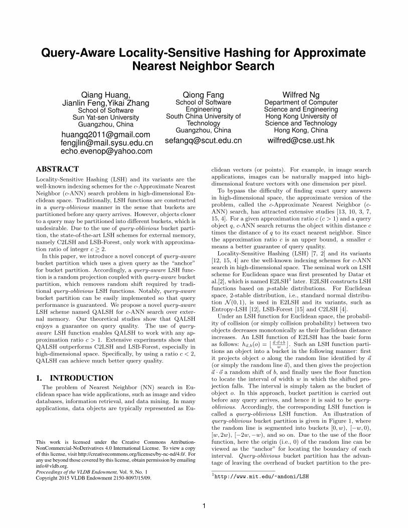
Motivated by the limitations of query-oblivious bucketpartition, we propose a novel concept of query-aware bucketpartition and develop novel query-aware LSH functions ac-cordingly. Given a pre-specified bucket width w, a hashfunction h~a(o) = ~a · ~o first projects object o along the ran-dom line ~a as before. When a query q arrives, we computethe projection of q (i.e., h~a(q)) and take the query projection(or simply the query) as the “anchor” for bucket partition.Specifically, the interval [h~a(q)− w

2, h~a(q)+ w

2], i.e., a bucket

of width w centered at h~a(q) (or simply at q), is first im-posed along the random line ~a. And if necessary, we canimpose buckets with any larger bucket width, in the samemanner of using the query as the “anchor”. This approachof bucket partition is said to be query-aware. In Section 3,we show that the hash function h~a(o) coupled with query-aware bucket partition is indeed locality-sensitive, and henceis called a query-aware LSH function. An example of query-aware bucket partition is illustrated in Figure 2, where h(q)evenly splits the buckets into two half-buckets of width w

2.

By applying the query-aware bucket partition, o1 and q arepartitioned into the same bucket, the undesirable situationillustrated in Figure 1 is then avoided.

Notice that random shift is not necessary for query-awarebucket partition. Thus, compared to query-oblivious LSHfunctions, query-aware LSH functions are simpler to com-pute. However, we need to dynamically do query-awarebucket partition. Given a query-aware LSH function h~a(o) =~a ·~o, in the pre-processing step, we compute the projectionsof all the data objects along the random line, and indexall the data projections by a B+-tree. When a query ob-

ject q arrives, we compute the query projection and usethe B+-tree to locate objects falling in the interval [h~a(q)−w2, h~a(q) + w

2]. And if required by our search algorithm, we

can gradually locate data objects even farther away fromthe query, just like performing a B+-tree range search. Inother words, we do not need to physically partition the wholerandom line at all. Therefore, the overhead of query-awarebucket partition is affordable.

Based on query-aware LSH functions, we propose a novelQuery-Aware LSH scheme called QALSH for c-ANN searchin high-dimensional Euclidean space. Interestingly, as ana-lyzed in Section 5.1, query-aware bucket partition enablesQALSH to work with any c > 1. In this paper, we alsodevelop a novel approach to setting the bucket width w au-tomatically, as shown in Section 5.3. In contrast, the state-of-the-art query-oblivious LSH schemes depend on manuallysetting w. For example, both E2LSH and LSB-Forest man-ually set w = 4.0, while C2LSH manually sets w = 1.0.

In summary, we introduce a novel concept of query-awarebucket partition and develop novel query-aware LSH func-tions accordingly. We propose a novel query-aware LSHscheme QALSH for high-dimensional c-ANN search over ex-ternal memory. QALSH works with any approximation ra-tio c > 1 and enjoys a theoretical guarantee on query qual-ity. QALSH also solves the problem of c-approximate k-nearest neighbors (c-k-ANN) search. Extensive experimentson four real datasets show that in high-dimensional Eu-clidean space QALSH outperforms C2LSH and LSB-Forestwhich also have guarantee on query quality.

The rest of this paper is organized as follows. We firstdiscuss preliminaries in Section 2. Then we introduce thequery-aware LSH family in Section 3. The QALSH scheme ispresented in Section 4 and its theoretical analysis is given inSection 5. Experimental studies are presented in Section 6.Related work is discussed in Section 7. Finally, we concludeour work in Section 8.

2. PRELIMINARIES

2.1 Problem SettingLet D be a database of n data objects in d-dimensional

Euclidean space Rd and let ‖o1, o2‖ denote the Euclideandistance between two objects o1 and o2. Given a queryobject q in Rd and an approximation ratio c (c > 1), c-ANN search is to find an object o ∈ D such that ‖o, q‖ ≤c‖o∗, q‖, where o∗ is the exact NN of q in D. Similarly, c-k-ANN is to find k objects oi ∈ D (1 ≤ i ≤ k) such that‖oi, q‖ ≤ c‖o∗i , q‖, where o∗i is the exact i-th NN of q in D.

2.2 Query-Oblivious LSH FamilyA family of LSH functions is able to partition “closer” ob-

jects into the same bucket with an accordingly higher prob-ability. If two objects o and q are partitioned into the samebucket by a hash function h, we say o and q collide under h.Formally, an LSH function family (or simply an LSH family)in Euclidean space is defined as:

Definition 1. Given a search radius r and approximationratio c, an LSH function family H = {h : Rd → U} is saidto be (r, cr, p1, p2)-sensitive, if, for any o, q ∈ Rd we have

• if ‖o, q‖ ≤ r, then PrH [o and q collide under h] ≥ p1;

• if ‖o, q‖ > cr, then PrH [o and q collide under h] ≤ p2.

2

where c > 1 and p1 > p2. For ease of reference, p1 andp2 are called positively-colliding probability and negatively-colliding probability, respectively.

A query-oblivious LSH family is an LSH family H ={h : Rd → Z} where each hash function h exploits query-oblivious bucket partition, i.e., buckets in the hash table ofh are statically determined before any query arrives. Nor-mally, for a query-oblivious LSH function h, two objects oand q collide under h means h(o) = h(q), where h(o) identi-fies the bucket of o. A typical query-oblivious LSH functionis formally defined as follows [2].

h~a,b(o) =

⌊~a · ~o+ b

w

⌋, (1)

where ~o is a d-dimensional Euclidean vector representingobject o, ~a is a d-dimensional random vector with each en-try drawn independently from standard normal distributionN (0, 1). w is the pre-specified bucket width, and b is a realnumber uniformly drawn from [0, w).

For two objects o1 and o2, and a uniformly randomly cho-sen hash function h~a,b, let s = ‖o1, o2‖, and then their col-lision probability is computed as follows [2]:

ξ(s) = Pr~a,b[h~a,b(o1) = h~a,b(o2)]=

∫ w0

1sf2( t

s)(1− t

w) dt

(2)

where f2(x) = 2√2πe−

x2

2 . For a fixed w, ξ(s) decreases

monotonically as s increases. With ξ1 = ξ(r) and ξ2 = ξ(cr),the family of hash functions h~a,b is (r, cr, ξ1, ξ2)-sensitive.Specifically, if we set r = 1 and cr = c, we have Lemma 1 asfollows [2] :

Lemma 1. The query-oblivious LSH family identified byEquation 1 is (1, c, ξ1, ξ2)-sensitive, where ξ1 = ξ(1) andξ2 = ξ(c).

3. QUERY-AWARE LSH FAMILYIn this section we first introduce the concept of query-

aware LSH functions. Then we make a computational com-parison of positively- and negatively-colliding probabilitiesbetween query-oblivious and query-aware LSH families. Fi-nally, we show that query-aware LSH family is able to sup-port virtual rehashing in a simple and quick manner.

3.1 (1, c, p1, p2)-sensitive LSH FamilyConstructing LSH functions in a query-aware manner con-

sists of two steps: random projection and query-aware bucketpartition. Formally, a query-aware hash function h~a(o) :Rd → R maps a d-dimensional object ~o to a number alongthe real line identified by a random vector ~a, whose entriesare drawn independently from N (0, 1). For a fixed ~a, thecorresponding hash function h~a(o) is defined as follows:

h~a(o) = ~a · ~o (3)

For all the data objects, their projections along the ran-dom line ~a are computed in the pre-processing step. Whena query object q arrives, we obtain the query projection bycomputing h~a(q). Then, we use the query as the “anchor”to locate the anchor bucket with width w (defined by h~a(·)),i.e., the interval [h~a(q) − w

2, h~a(q) + w

2]. If the projection

of an object o (i.e., h~a(o)), falls in the anchor bucket withwidth w, i.e., |h~a(o) − h~a(q)| ≤ w

2, we say o collides with q

under h~a.

We now show that the family of hash functions h~a(o) cou-pled with query-aware bucket partition is locality-sensitive.In this sense, each h~a(o) in the family is said to be a query-aware LSH function. For objects o and q, let s = ‖o, q‖.Due to the stability of standard normal distribution N (0, 1),we have that (~a · ~o − ~a · ~q) is distributed as sX, whereX is a random variable drawn from N (0, 1) [2]. Let ϕ(x)be the probability density function (PDF) of N (0, 1), i.e.,

ϕ(x) = 1√2πe−

x2

2 . The collision probability between o and

q under h~a is computed as follows:

p(s) = Pr~a[|h~a(o)− h~a(q)| ≤ w2

] = Pr[|sX| ≤ w2

]

= Pr[− w2s≤ X ≤ w

2s] =

∫ w2s− w

2sϕ(x) dx

(4)

Accordingly, we have Lemma 2 as follows:

Lemma 2. The query-aware hash family of all the hashfunctions h~a(o) that are identified by Equation 3 and coupledwith query-aware bucket partition is (1, c, p1, p2)-sensitive,where p1 = p(1) and p2 = p(c).

Proof. Referring to Equation 4 , a simple calculationshows that p(s) = 1 − 2norm(− w

2s), where norm(x) =∫ x

−∞ ϕ(t) dt. Note that norm(x) is simply the cumulative

distribution function (CDF) ofN (0, 1), which increases mono-tonically as x increases. For a fixed w, norm(− w

2s) in-

creases monotonically as s increases, and hence p(s) de-creases monotonically as s increases. Therefore, accordingto Definition 1, the query-aware hash family identified byEquation 3, is (1, c, p1, p2)-sensitive, where p1 = p(1) andp2 = p(c), respectively.

3.2 Comparison of Colliding ProbabilitiesThe effectiveness of an (r, cr, p1, p2)-sensitive hash family

depends on the difference between the positively-collidingprobability and negatively-colliding probability, i.e., (p1 −p2), since the difference measures the degree that positively-colliding data objects of a query q can be discriminatedfrom negatively-colliding ones. We now show that the novelquery-aware hash family leads to larger (p1−p2) under typi-cal settings of bucket width w. For query-aware LSH family,from the proof of Lemma 2, we have p1 = 1 − 2norm(−w

2)

and p2 = 1 − 2norm(− w2c

). For query-oblivious LSH fam-

ily, we have ξ1 = 1− 2norm(−w)− 2√2πw

(1− e−(w2/2)) and

ξ2 = 1− 2norm(−w/c)− 2√2πw/c

(1− e−(w2/2c2)) [2].

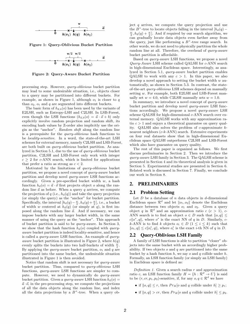
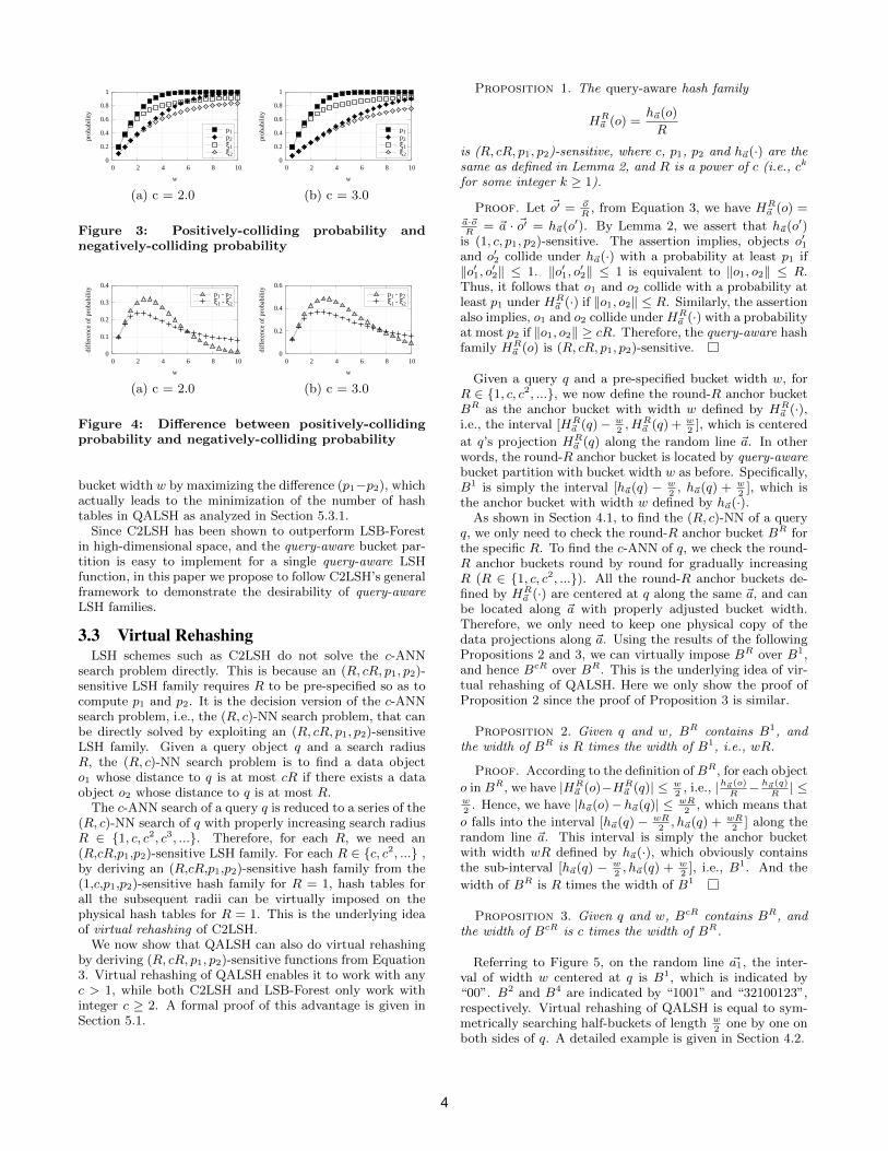
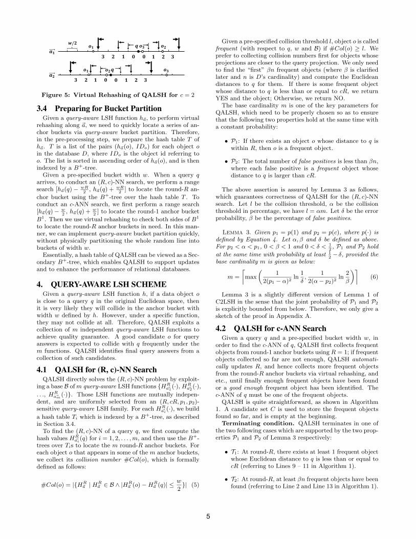
Bucket width w is a critical parameter of an LSH function.While E2LSH and LSB-Forest manually set w = 4.0, C2LSHmanually sets w = 1.0. For w in the range [0, 10], startingfrom 0.5 and with a step of 0.5, we show the variations of thecolliding probabilities p1, p2, ξ1, and ξ2 for two different cvalues in Figure 3. We find that all the colliding probabilitiesmonotonically increase as w increases, and get very close to 1as w gets close to 10. In addition, p1 and p2 are consistentlylarger than ξ1 and ξ2, respectively. Thus, we also showthe two differences (p1 − p2) and (ξ1 − ξ2) with respect tow in Figure 4. We have two interesting observations: (1)(p1−p2) is larger than (ξ1−ξ2) under typical bucket widths,namely w = 4.0 and w = 1.0. (2) Both (p1 − p2) and(ξ1−ξ2) tend to have maximum values in the w range [0, 10].Observation (1) indicates that our novel query-aware LSHfamily can be used to improve the performance of query-oblivious LSH schemes such as C2LSH by leveraging a larger(p1 − p2). Observation (2) inspires us to automatically set

3

0

0.2

0.4

0.6

0.8

1

0 2 4 6 8 10

pro

bab

ilit

y

w

p1p2

ξ1ξ2

(a) c = 2.0

0

0.2

0.4

0.6

0.8

1

0 2 4 6 8 10

pro

bab

ilit

y

w

p1p2

ξ1ξ2

(b) c = 3.0

Figure 3: Positively-colliding probability andnegatively-colliding probability

0

0.1

0.2

0.3

0.4

0 2 4 6 8 10

dif

fere

nce

of

pro

bab

ilit

y

w

p1 - p2ξ1 - ξ2

(a) c = 2.0

0

0.2

0.4

0.6

0 2 4 6 8 10

dif

fere

nce

of

pro

bab

ilit

y

w

p1 - p2ξ1 - ξ2

(b) c = 3.0

Figure 4: Difference between positively-collidingprobability and negatively-colliding probability

bucket width w by maximizing the difference (p1−p2), whichactually leads to the minimization of the number of hashtables in QALSH as analyzed in Section 5.3.1.

Since C2LSH has been shown to outperform LSB-Forestin high-dimensional space, and the query-aware bucket par-tition is easy to implement for a single query-aware LSHfunction, in this paper we propose to follow C2LSH’s generalframework to demonstrate the desirability of query-awareLSH families.

3.3 Virtual RehashingLSH schemes such as C2LSH do not solve the c-ANN

search problem directly. This is because an (R, cR, p1, p2)-sensitive LSH family requires R to be pre-specified so as tocompute p1 and p2. It is the decision version of the c-ANNsearch problem, i.e., the (R, c)-NN search problem, that canbe directly solved by exploiting an (R, cR, p1, p2)-sensitiveLSH family. Given a query object q and a search radiusR, the (R, c)-NN search problem is to find a data objecto1 whose distance to q is at most cR if there exists a dataobject o2 whose distance to q is at most R.

The c-ANN search of a query q is reduced to a series of the(R, c)-NN search of q with properly increasing search radiusR ∈ {1, c, c2, c3, ...}. Therefore, for each R, we need an(R,cR,p1,p2)-sensitive LSH family. For each R ∈ {c, c2, ...} ,by deriving an (R,cR,p1,p2)-sensitive hash family from the(1,c,p1,p2)-sensitive hash family for R = 1, hash tables forall the subsequent radii can be virtually imposed on thephysical hash tables for R = 1. This is the underlying ideaof virtual rehashing of C2LSH.

We now show that QALSH can also do virtual rehashingby deriving (R, cR, p1, p2)-sensitive functions from Equation3. Virtual rehashing of QALSH enables it to work with anyc > 1, while both C2LSH and LSB-Forest only work withinteger c ≥ 2. A formal proof of this advantage is given inSection 5.1.

Proposition 1. The query-aware hash family

HR~a (o) =

h~a(o)

R

is (R, cR, p1, p2)-sensitive, where c, p1, p2 and h~a(·) are thesame as defined in Lemma 2, and R is a power of c (i.e., ck

for some integer k ≥ 1).

Proof. Let ~o′ = ~oR

, from Equation 3, we have HR~a (o) =

~a·~oR

= ~a · ~o′ = h~a(o′). By Lemma 2, we assert that h~a(o′)is (1, c, p1, p2)-sensitive. The assertion implies, objects o′1and o′2 collide under h~a(·) with a probability at least p1 if‖o′1, o′2‖ ≤ 1. ‖o′1, o′2‖ ≤ 1 is equivalent to ‖o1, o2‖ ≤ R.Thus, it follows that o1 and o2 collide with a probability atleast p1 under HR

~a (·) if ‖o1, o2‖ ≤ R. Similarly, the assertionalso implies, o1 and o2 collide underHR

~a (·) with a probabilityat most p2 if ‖o1, o2‖ ≥ cR. Therefore, the query-aware hashfamily HR

~a (o) is (R, cR, p1, p2)-sensitive.

Given a query q and a pre-specified bucket width w, forR ∈ {1, c, c2, ...}, we now define the round-R anchor bucketBR as the anchor bucket with width w defined by HR

~a (·),i.e., the interval [HR

~a (q)− w2, HR

~a (q) + w2

], which is centered

at q’s projection HR~a (q) along the random line ~a. In other

words, the round-R anchor bucket is located by query-awarebucket partition with bucket width w as before. Specifically,B1 is simply the interval [h~a(q) − w

2, h~a(q) + w

2], which is

the anchor bucket with width w defined by h~a(·).As shown in Section 4.1, to find the (R, c)-NN of a query

q, we only need to check the round-R anchor bucket BR forthe specific R. To find the c-ANN of q, we check the round-R anchor buckets round by round for gradually increasingR (R ∈ {1, c, c2, ...}). All the round-R anchor buckets de-fined by HR

~a (·) are centered at q along the same ~a, and canbe located along ~a with properly adjusted bucket width.Therefore, we only need to keep one physical copy of thedata projections along ~a. Using the results of the followingPropositions 2 and 3, we can virtually impose BR over B1,and hence BcR over BR. This is the underlying idea of vir-tual rehashing of QALSH. Here we only show the proof ofProposition 2 since the proof of Proposition 3 is similar.

Proposition 2. Given q and w, BR contains B1, andthe width of BR is R times the width of B1, i.e., wR.

Proof. According to the definition of BR, for each object

o in BR, we have |HR~a (o)−HR

~a (q)| ≤ w2

, i.e., |h~a(o)R− h~a(q)

R| ≤

w2

. Hence, we have |h~a(o)−h~a(q)| ≤ wR2

, which means that

o falls into the interval [h~a(q) − wR2, h~a(q) + wR

2] along the

random line ~a. This interval is simply the anchor bucketwith width wR defined by h~a(·), which obviously containsthe sub-interval [h~a(q) − w

2, h~a(q) + w

2], i.e., B1. And the

width of BR is R times the width of B1

Proposition 3. Given q and w, BcR contains BR, andthe width of BcR is c times the width of BR.

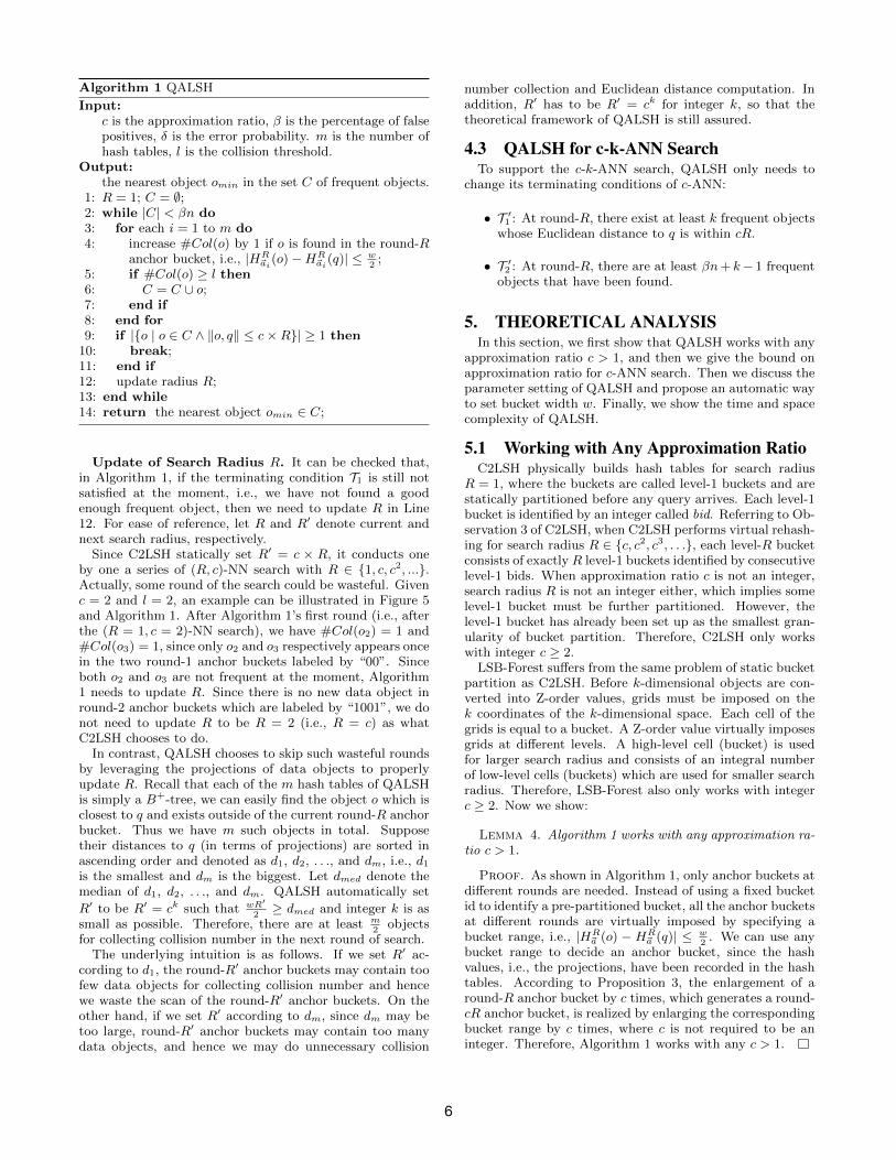
Referring to Figure 5, on the random line ~a1, the inter-val of width w centered at q is B1, which is indicated by“00”. B2 and B4 are indicated by “1001” and “32100123”,respectively. Virtual rehashing of QALSH is equal to sym-metrically searching half-buckets of length w

2one by one on

both sides of q. A detailed example is given in Section 4.2.

4

1

𝒂𝟏

𝒂𝟐

𝒐𝟐𝒒 𝒐𝟑𝒐𝟏

𝒐𝟐𝒒 𝒐𝟑𝒐𝟏

𝟎 𝟏 𝟑𝟐𝟑 𝟏𝟐

𝟎 𝟏 𝟑𝟐𝟑 𝟏𝟐

𝟎

𝟎

𝒘/𝟐

Figure 5: Virtual Rehashing of QALSH for c = 2

3.4 Preparing for Bucket PartitionGiven a query-aware LSH function h~a, to perform virtual

rehashing along ~a, we need to quickly locate a series of an-chor buckets via query-aware bucket partition. Therefore,in the pre-processing step, we prepare the hash table T ofh~a. T is a list of the pairs (h~a(o), IDo) for each object oin the database D, where IDo is the object id referring too. The list is sorted in ascending order of h~a(o), and is thenindexed by a B+-tree.

Given a pre-specified bucket width w. When a query qarrives, to conduct an (R, c)-NN search, we perform a rangesearch [h~a(q)− wR

2, h~a(q) + wR

2] to locate the round-R an-

chor bucket using the B+-tree over the hash table T . Toconduct an c-ANN search, we first perform a range search[h~a(q)− w

2, h~a(q) + w

2] to locate the round-1 anchor bucket

B1. Then we use virtual rehashing to check both sides of B1

to locate the round-R anchor buckets in need. In this man-ner, we can implement query-aware bucket partition quickly,without physically partitioning the whole random line intobuckets of width w.

Essentially, a hash table of QALSH can be viewed as a Sec-ondary B+-tree, which enables QALSH to support updatesand to enhance the performance of relational databases.

4. QUERY-AWARE LSH SCHEMEGiven a query-aware LSH function h, if a data object o

is close to a query q in the original Euclidean space, thenit is very likely they will collide in the anchor bucket withwidth w defined by h. However, under a specific function,they may not collide at all. Therefore, QALSH exploits acollection of m independent query-aware LSH functions toachieve quality guarantee. A good candidate o for queryanswers is expected to collide with q frequently under them functions. QALSH identifies final query answers from acollection of such candidates.

4.1 QALSH for (R, c)-NN SearchQALSH directly solves the (R, c)-NN problem by exploit-

ing a base B ofm query-aware LSH functions {HR~a1

(·), HR~a2

(·),. . ., HR

~am(·)}. Those LSH functions are mutually indepen-

dent, and are uniformly selected from an (R, cR, p1, p2)-sensitive query-aware LSH family. For each HR

~ai(·), we build

a hash table Ti which is indexed by a B+-tree, as describedin Section 3.4.

To find the (R, c)-NN of a query q, we first compute thehash values HR

~ai(q) for i = 1, 2, . . . ,m, and then use the B+-

trees over Tis to locate the m round-R anchor buckets. Foreach object o that appears in some of the m anchor buckets,we collect its collision number #Col(o), which is formallydefined as follows:

#Col(o) = |{HR~a | HR

~a ∈ B ∧ |HR~a (o)−HR

~a (q)| ≤ w

2}| (5)

Given a pre-specified collision threshold l, object o is calledfrequent (with respect to q, w and B) if #Col(o) ≥ l. Weprefer to collecting collision numbers first for objects whoseprojections are closer to the query projection. We only needto find the “first” βn frequent objects (where β is clarifiedlater and n is D’s cardinality) and compute the Euclideandistances to q for them. If there is some frequent objectwhose distance to q is less than or equal to cR, we returnYES and the object; Otherwise, we return NO.

The base cardinality m is one of the key parameters forQALSH, which need to be properly chosen so as to ensurethat the following two properties hold at the same time witha constant probability:

• P1: If there exists an object o whose distance to q iswithin R, then o is a frequent object.

• P2: The total number of false positives is less than βn,where each false positive is a frequent object whosedistance to q is larger than cR.

The above assertion is assured by Lemma 3 as follows,which guarantees correctness of QALSH for the (R, c)-NNsearch. Let l be the collision threshold, α be the collisionthreshold in percentage, we have l = αm. Let δ be the errorprobability, β be the percentage of false positives.

Lemma 3. Given p1 = p(1) and p2 = p(c), where p(·) isdefined by Equation 4. Let α, β and δ be defined as above.For p2 < α < p1, 0 < β < 1 and 0 < δ < 1

2, P1 and P2 hold

at the same time with probability at least 12− δ, provided the

base cardinality m is given as below:

m =

⌈max

(1

2(p1 − α)2ln

1

δ,

1

2(α− p2)2ln

2

β

)⌉(6)

Lemma 3 is a slightly different version of Lemma 1 ofC2LSH in the sense that the joint probability of P1 and P2

is explicitly bounded from below. Therefore, we only give asketch of the proof in Appendix A.

4.2 QALSH for c-ANN SearchGiven a query q and a pre-specified bucket width w, in

order to find the c-ANN of q, QALSH first collects frequentobjects from round-1 anchor buckets using R = 1; if frequentobjects collected so far are not enough, QALSH automati-cally updates R, and hence collects more frequent objectsfrom the round-R anchor buckets via virtual rehashing, andetc., until finally enough frequent objects have been foundor a good enough frequent object has been identified. Thec-ANN of q must be one of the frequent objects.

QALSH is quite straightforward, as shown in Algorithm1. A candidate set C is used to store the frequent objectsfound so far, and is empty at the beginning.

Terminating condition. QALSH terminates in one ofthe two following cases which are supported by the two prop-erties P1 and P2 of Lemma 3 respectively:

• T1: At round-R, there exists at least 1 frequent objectwhose Euclidean distance to q is less than or equal tocR (referring to Lines 9 – 11 in Algorithm 1).

• T2: At round-R, at least βn frequent objects have beenfound (referring to Line 2 and Line 13 in Algorithm 1).

5

Algorithm 1 QALSH

Input:c is the approximation ratio, β is the percentage of falsepositives, δ is the error probability. m is the number ofhash tables, l is the collision threshold.

Output:the nearest object omin in the set C of frequent objects.

1: R = 1; C = ∅;2: while |C| < βn do3: for each i = 1 to m do4: increase #Col(o) by 1 if o is found in the round-R

anchor bucket, i.e., |HR~ai

(o)−HR~ai

(q)| ≤ w2

;5: if #Col(o) ≥ l then6: C = C ∪ o;7: end if8: end for9: if |{o | o ∈ C ∧ ‖o, q‖ ≤ c×R}| ≥ 1 then

10: break;11: end if12: update radius R;13: end while14: return the nearest object omin ∈ C;

Update of Search Radius R. It can be checked that,in Algorithm 1, if the terminating condition T1 is still notsatisfied at the moment, i.e., we have not found a goodenough frequent object, then we need to update R in Line12. For ease of reference, let R and R′ denote current andnext search radius, respectively.

Since C2LSH statically set R′ = c × R, it conducts oneby one a series of (R, c)-NN search with R ∈ {1, c, c2, ...}.Actually, some round of the search could be wasteful. Givenc = 2 and l = 2, an example can be illustrated in Figure 5and Algorithm 1. After Algorithm 1’s first round (i.e., afterthe (R = 1, c = 2)-NN search), we have #Col(o2) = 1 and#Col(o3) = 1, since only o2 and o3 respectively appears oncein the two round-1 anchor buckets labeled by “00”. Sinceboth o2 and o3 are not frequent at the moment, Algorithm1 needs to update R. Since there is no new data object inround-2 anchor buckets which are labeled by “1001”, we donot need to update R to be R = 2 (i.e., R = c) as whatC2LSH chooses to do.

In contrast, QALSH chooses to skip such wasteful roundsby leveraging the projections of data objects to properlyupdate R. Recall that each of the m hash tables of QALSHis simply a B+-tree, we can easily find the object o which isclosest to q and exists outside of the current round-R anchorbucket. Thus we have m such objects in total. Supposetheir distances to q (in terms of projections) are sorted inascending order and denoted as d1, d2, . . ., and dm, i.e., d1is the smallest and dm is the biggest. Let dmed denote themedian of d1, d2, . . ., and dm. QALSH automatically set

R′ to be R′ = ck such that wR′

2≥ dmed and integer k is as

small as possible. Therefore, there are at least m2

objectsfor collecting collision number in the next round of search.

The underlying intuition is as follows. If we set R′ ac-cording to d1, the round-R′ anchor buckets may contain toofew data objects for collecting collision number and hencewe waste the scan of the round-R′ anchor buckets. On theother hand, if we set R′ according to dm, since dm may betoo large, round-R′ anchor buckets may contain too manydata objects, and hence we may do unnecessary collision

number collection and Euclidean distance computation. Inaddition, R′ has to be R′ = ck for integer k, so that thetheoretical framework of QALSH is still assured.

4.3 QALSH for c-k-ANN SearchTo support the c-k-ANN search, QALSH only needs to

change its terminating conditions of c-ANN:

• T ′1 : At round-R, there exist at least k frequent objectswhose Euclidean distance to q is within cR.

• T ′2 : At round-R, there are at least βn+ k− 1 frequentobjects that have been found.

5. THEORETICAL ANALYSISIn this section, we first show that QALSH works with any

approximation ratio c > 1, and then we give the bound onapproximation ratio for c-ANN search. Then we discuss theparameter setting of QALSH and propose an automatic wayto set bucket width w. Finally, we show the time and spacecomplexity of QALSH.

5.1 Working with Any Approximation RatioC2LSH physically builds hash tables for search radius

R = 1, where the buckets are called level-1 buckets and arestatically partitioned before any query arrives. Each level-1bucket is identified by an integer called bid. Referring to Ob-servation 3 of C2LSH, when C2LSH performs virtual rehash-ing for search radius R ∈ {c, c2, c3, . . .}, each level-R bucketconsists of exactly R level-1 buckets identified by consecutivelevel-1 bids. When approximation ratio c is not an integer,search radius R is not an integer either, which implies somelevel-1 bucket must be further partitioned. However, thelevel-1 bucket has already been set up as the smallest gran-ularity of bucket partition. Therefore, C2LSH only workswith integer c ≥ 2.

LSB-Forest suffers from the same problem of static bucketpartition as C2LSH. Before k-dimensional objects are con-verted into Z-order values, grids must be imposed on thek coordinates of the k-dimensional space. Each cell of thegrids is equal to a bucket. A Z-order value virtually imposesgrids at different levels. A high-level cell (bucket) is usedfor larger search radius and consists of an integral numberof low-level cells (buckets) which are used for smaller searchradius. Therefore, LSB-Forest also only works with integerc ≥ 2. Now we show:

Lemma 4. Algorithm 1 works with any approximation ra-tio c > 1.

Proof. As shown in Algorithm 1, only anchor buckets atdifferent rounds are needed. Instead of using a fixed bucketid to identify a pre-partitioned bucket, all the anchor bucketsat different rounds are virtually imposed by specifying abucket range, i.e., |HR

~a (o) − HR~a (q)| ≤ w

2. We can use any

bucket range to decide an anchor bucket, since the hashvalues, i.e., the projections, have been recorded in the hashtables. According to Proposition 3, the enlargement of around-R anchor bucket by c times, which generates a round-cR anchor bucket, is realized by enlarging the correspondingbucket range by c times, where c is not required to be aninteger. Therefore, Algorithm 1 works with any c > 1.

6

5.2 Bound on Approximation RatioFor c-ANN search, we now present the bound on approx-

imation ratio for Algorithm 1.

Theorem 1. Algorithm 1 returns a c2-approximate NNwith probability at least 1

2− δ.

Since both QALSH and C2LSH use the technique of vir-tual rehashing, this theorem is a stronger version of Theorem1 of C2LSH in the sense that the probability in this theo-rem is explicitly bounded from below. This theorem simplyfollows from the combination of Theorem 1 of C2LSH andLemma 3 of QALSH.

5.3 Parameter SettingsThe accuracy of QALSH is controlled by error probability

δ, approximation ratio c and false positive percentage β,where δ, c and β are constants specified by users. δ controlsthe success rate of any LSH-based method for c-ANN search.In this paper, we set δ = 1

e. A smaller c means a higher

accuracy. Intuitively, a bigger β allows C2LSH and QALSHto check more frequent objects, and hence enables them toachieve a better search quality, with higher costs in terms ofrandom I/Os. Similar to C2LSH, QALSH sets β = 100/nto restrict the number of random I/Os.

We now consider the base cardinality m, collision thresh-old percentage α and collision threshold l. Referring to

Equation 6 of Lemma 3, let m1 =⌈

12(p1−α)2

ln 1δ

⌉and m2 =⌈

12(α−p2)2

ln 2β

⌉, we have m = max(m1,m2). Since p2 <

α < p1, m1 increases monotonically with α and m2 de-creases monotonically with α. Since m = max(m1,m2), mis smallest when m1 = m2. Then, α can be determined by:

α =η · p1 + p2

1 + η, where η =

√ln 2

β

ln 1δ

(7)

Replacing α in m1 by Equation 7, we have:

m =

(√

ln 2β

+√

ln 1δ

)22(p1 − p2)2

(8)

After setting the values of m and α, we compute the in-teger collision threshold l as follows:

l = dαme (9)

The base cardinality m is simply the number of hash ta-bles in QALSH. A small m leads to small time and spaceoverhead in QALSH, as shown in Section 5.4. However, mmust be set to satisfy the requirement of Lemma 3 for qual-ity guarantee. It follows from Equation 8 that m decreasesmonotonically with the difference (p1−p2) for fixed δ and β.From Section 3.2, we know there is a value of w in the range[0, 10] to maximize (p1 − p2). Both E2LSH and LSB-Forestmanually set bucket width w = 4.0, while C2LSH manuallyset w = 1.0. In the next section, we propose to automati-cally decide w so as to minimize the base cardinality m.

5.3.1 Automatically Setting w by Minimizing mThe strategy of minimizing m is to select the value of w

that maximizes the difference (p1 − p2). Formally, we haveLemma 5 to minimize m.

Lemma 5. Suppose δ and β are user-specified constants,for any approximation ratio c > 1, the base cardinality m ofQALSH is minimized by setting

w =

√8c2 ln c

c2 − 1(10)

Proof. Let µ(w) = p1 − p2. From Equation 4, we have:

µ(w) = p1 − p2=

∫ w2−w

2

1√2πe−

t2

2 dt−∫ w

2c− w

2c

1√2πe−

t2

2 dt

= 2√2π

∫ w2−∞ e

− t2

2 dt− 2√2π

∫ w2c−∞ e

− t2

2 dt

Using the basic techniques of calculus, we take the deriva-tive and obtain the following equation:

µ′(w) = 1√2π

(e−w2

8 − 1c· e−

w2

8c2 )

Let µ′(w) = 0. Since w > 0 and c > 1, we have the

expression w∗ =√

8c2 ln cc2−1

. When 0 < w < w∗, µ′(w) > 0

and when w > w∗, µ′(w) < 0. Thus, µ(w) monotonically in-creases with w for 0 < w < w∗, and monotonically decreaseswith w for w > w∗. Therefore, µ(w) = p1 − p2 achieves itsmaximum value when w = w∗. From Equation 8, m de-creases monotonically with the difference (p1 − p2) since βand δ are constants. Thus, m achieves its minimum valuewhen w = w∗. Since Equation 8 is derived from Lemma 3,the minimum value of m satisfies the quality guarantee.

5.4 Time and Space ComplexitySince we set β = 100

n, βn is constant. From Equations 8

and 9, we have m = O(logn) and l = O(logn), respectively.The time cost of QALSH consists of four parts: First,

computing the projection of a query for m hash tables costsmd = O(d logn); Second, locating the m round-1 anchorbuckets in B+-tree costs m logn = O((logn)2); Third, inthe worst case, finding the frequent objects as candidatesneeds to do collision counting for all the n objects over eachhash table, which costs ln = O(n logn); Finally, calculatingEuclidean distance for candidates costs βnd = O(d). There-fore, the time complexity of QALSH is O(d logn+(logn)2 +n logn+ d) = O(d logn+ n logn).

The space complexity of QALSH consists of two parts:the space of dataset O(nd) and the space of index mn =O(n logn) for m hash tables which store n data objects’id and projection. Thus, the total space consumption ofQALSH is O(nd+ n logn).

6. EXPERIMENTSIn this section, we study the performance of QALSH using

four real datasets. Since QALSH has quality guarantee andis designed for external memory, we take two state-of-the-art schemes of the same kind as the benchmark, namely,LSB-Forest and C2LSH.

6.1 Experiment Setup

6.1.1 Benchmark Methods

• LSB-Forest. LSB-Forest uses a set of L LSB-Trees toachieve quality guarantee, which has a success probabil-ity at least 1

2− 1

e. LSB-Forest requires 2L buffer pages

for c-ANN search. Since LSB-Forest has been shown to

7

outperform iDistance [8] and MEDRANK [3], they areomitted for comparison here.

• C2LSH. C2LSH is most related to QALSH. It requires abuffer of 2m pages for c-ANN search, where m is the num-ber of hash tables used in C2LSH. We consider C2LSHwith l as the collision threshold, as only under this case ithas quality guarantee.

Our method is implemented in C++. All methods arecompiled with gcc 4.8 with -O3. All experiments were doneon a PC with Intel Core i7-2670M 2.20GHz CPU, 8 GBmemory and 1 TB hard disk, running Linux 3.11.

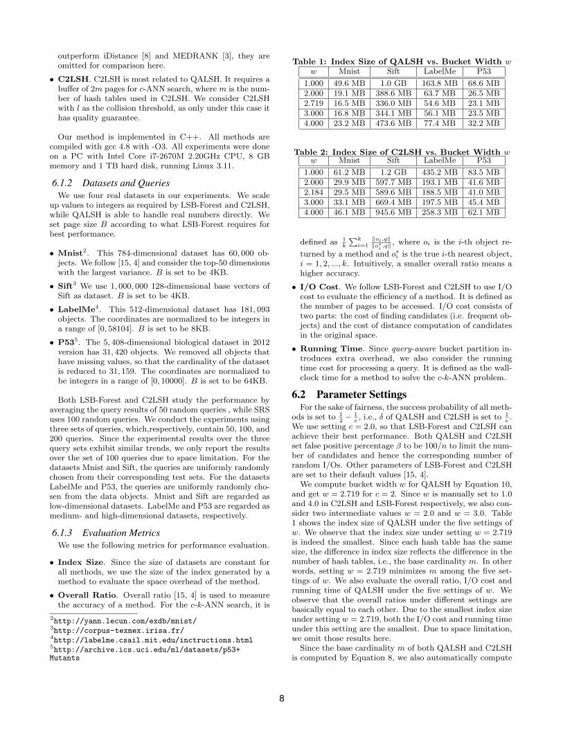
6.1.2 Datasets and QueriesWe use four real datasets in our experiments. We scale

up values to integers as required by LSB-Forest and C2LSH,while QALSH is able to handle real numbers directly. Weset page size B according to what LSB-Forest requires forbest performance.

• Mnist2. This 784-dimensional dataset has 60, 000 ob-jects. We follow [15, 4] and consider the top-50 dimensionswith the largest variance. B is set to be 4KB.

• Sift3 We use 1, 000, 000 128-dimensional base vectors ofSift as dataset. B is set to be 4KB.

• LabelMe4. This 512-dimensional dataset has 181, 093objects. The coordinates are normalized to be integers ina range of [0, 58104]. B is set to be 8KB.

• P535. The 5, 408-dimensional biological dataset in 2012version has 31, 420 objects. We removed all objects thathave missing values, so that the cardinality of the datasetis reduced to 31, 159. The coordinates are normalized tobe integers in a range of [0, 10000]. B is set to be 64KB.

Both LSB-Forest and C2LSH study the performance byaveraging the query results of 50 random queries , while SRSuses 100 random queries. We conduct the experiments usingthree sets of queries, which,respectively, contain 50, 100, and200 queries. Since the experimental results over the threequery sets exhibit similar trends, we only report the resultsover the set of 100 queries due to space limitation. For thedatasets Mnist and Sift, the queries are uniformly randomlychosen from their corresponding test sets. For the datasetsLabelMe and P53, the queries are uniformly randomly cho-sen from the data objects. Mnist and Sift are regarded aslow-dimensional datasets. LabelMe and P53 are regarded asmedium- and high-dimensional datasets, respectively.

6.1.3 Evaluation MetricsWe use the following metrics for performance evaluation.

• Index Size. Since the size of datasets are constant forall methods, we use the size of the index generated by amethod to evaluate the space overhead of the method.

• Overall Ratio. Overall ratio [15, 4] is used to measurethe accuracy of a method. For the c-k-ANN search, it is

2http://yann.lecun.com/exdb/mnist/3http://corpus-texmex.irisa.fr/4http://labelme.csail.mit.edu/inctructions.html5http://archive.ics.uci.edu/ml/datasets/p53+Mutants

Table 1: Index Size of QALSH vs. Bucket Width ww Mnist Sift LabelMe P53

1.000 49.6 MB 1.0 GB 163.8 MB 68.6 MB2.000 19.1 MB 388.6 MB 63.7 MB 26.5 MB2.719 16.5 MB 336.0 MB 54.6 MB 23.1 MB3.000 16.8 MB 344.1 MB 56.1 MB 23.5 MB4.000 23.2 MB 473.6 MB 77.4 MB 32.2 MB

Table 2: Index Size of C2LSH vs. Bucket Width ww Mnist Sift LabelMe P53

1.000 61.2 MB 1.2 GB 435.2 MB 83.5 MB2.000 29.9 MB 597.7 MB 193.1 MB 41.6 MB2.184 29.5 MB 589.6 MB 188.5 MB 41.0 MB3.000 33.1 MB 669.4 MB 197.5 MB 45.4 MB4.000 46.1 MB 945.6 MB 258.3 MB 62.1 MB

defined as 1k

∑ki=1

‖oi,q‖‖o∗i ,q‖

, where oi is the i-th object re-

turned by a method and o∗i is the true i-th nearest object,i = 1, 2, ..., k. Intuitively, a smaller overall ratio means ahigher accuracy.

• I/O Cost. We follow LSB-Forest and C2LSH to use I/Ocost to evaluate the efficiency of a method. It is defined asthe number of pages to be accessed. I/O cost consists oftwo parts: the cost of finding candidates (i.e. frequent ob-jects) and the cost of distance computation of candidatesin the original space.

• Running Time. Since query-aware bucket partition in-troduces extra overhead, we also consider the runningtime cost for processing a query. It is defined as the wall-clock time for a method to solve the c-k-ANN problem.

6.2 Parameter SettingsFor the sake of fairness, the success probability of all meth-

ods is set to 12− 1

e, i.e., δ of QALSH and C2LSH is set to 1

e.

We use setting c = 2.0, so that LSB-Forest and C2LSH canachieve their best performance. Both QALSH and C2LSHset false positive percentage β to be 100/n to limit the num-ber of candidates and hence the corresponding number ofrandom I/Os. Other parameters of LSB-Forest and C2LSHare set to their default values [15, 4].

We compute bucket width w for QALSH by Equation 10,and get w = 2.719 for c = 2. Since w is manually set to 1.0and 4.0 in C2LSH and LSB-Forest respectively, we also con-sider two intermediate values w = 2.0 and w = 3.0. Table1 shows the index size of QALSH under the five settings ofw. We observe that the index size under setting w = 2.719is indeed the smallest. Since each hash table has the samesize, the difference in index size reflects the difference in thenumber of hash tables, i.e., the base cardinality m. In otherwords, setting w = 2.719 minimizes m among the five set-tings of w. We also evaluate the overall ratio, I/O cost andrunning time of QALSH under the five settings of w. Weobserve that the overall ratios under different settings arebasically equal to each other. Due to the smallest index sizeunder setting w = 2.719, both the I/O cost and running timeunder this setting are the smallest. Due to space limitation,we omit those results here.

Since the base cardinality m of both QALSH and C2LSHis computed by Equation 8, we also automatically compute

8

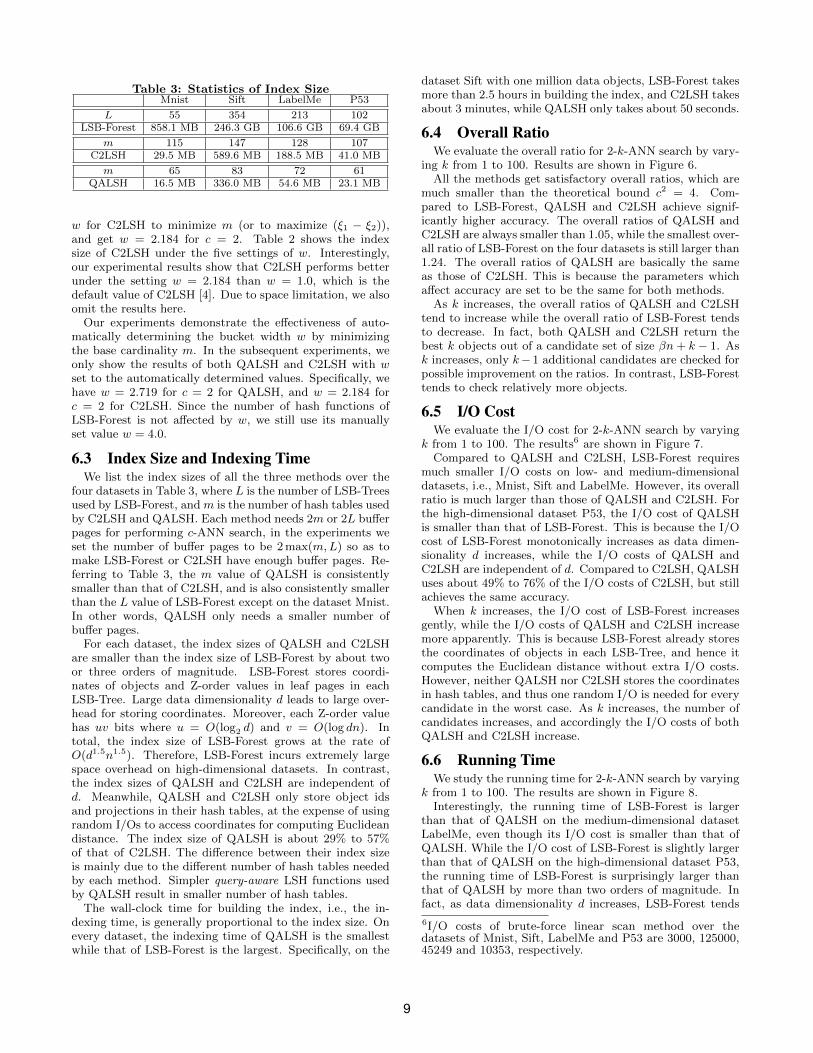
Table 3: Statistics of Index SizeMnist Sift LabelMe P53

L 55 354 213 102LSB-Forest 858.1 MB 246.3 GB 106.6 GB 69.4 GB

m 115 147 128 107C2LSH 29.5 MB 589.6 MB 188.5 MB 41.0 MB

m 65 83 72 61QALSH 16.5 MB 336.0 MB 54.6 MB 23.1 MB

w for C2LSH to minimize m (or to maximize (ξ1 − ξ2)),and get w = 2.184 for c = 2. Table 2 shows the indexsize of C2LSH under the five settings of w. Interestingly,our experimental results show that C2LSH performs betterunder the setting w = 2.184 than w = 1.0, which is thedefault value of C2LSH [4]. Due to space limitation, we alsoomit the results here.

Our experiments demonstrate the effectiveness of auto-matically determining the bucket width w by minimizingthe base cardinality m. In the subsequent experiments, weonly show the results of both QALSH and C2LSH with wset to the automatically determined values. Specifically, wehave w = 2.719 for c = 2 for QALSH, and w = 2.184 forc = 2 for C2LSH. Since the number of hash functions ofLSB-Forest is not affected by w, we still use its manuallyset value w = 4.0.

6.3 Index Size and Indexing TimeWe list the index sizes of all the three methods over the

four datasets in Table 3, where L is the number of LSB-Treesused by LSB-Forest, andm is the number of hash tables usedby C2LSH and QALSH. Each method needs 2m or 2L bufferpages for performing c-ANN search, in the experiments weset the number of buffer pages to be 2 max(m,L) so as tomake LSB-Forest or C2LSH have enough buffer pages. Re-ferring to Table 3, the m value of QALSH is consistentlysmaller than that of C2LSH, and is also consistently smallerthan the L value of LSB-Forest except on the dataset Mnist.In other words, QALSH only needs a smaller number ofbuffer pages.

For each dataset, the index sizes of QALSH and C2LSHare smaller than the index size of LSB-Forest by about twoor three orders of magnitude. LSB-Forest stores coordi-nates of objects and Z-order values in leaf pages in eachLSB-Tree. Large data dimensionality d leads to large over-head for storing coordinates. Moreover, each Z-order valuehas uv bits where u = O(log2 d) and v = O(log dn). Intotal, the index size of LSB-Forest grows at the rate ofO(d1.5n1.5). Therefore, LSB-Forest incurs extremely largespace overhead on high-dimensional datasets. In contrast,the index sizes of QALSH and C2LSH are independent ofd. Meanwhile, QALSH and C2LSH only store object idsand projections in their hash tables, at the expense of usingrandom I/Os to access coordinates for computing Euclideandistance. The index size of QALSH is about 29% to 57%of that of C2LSH. The difference between their index sizeis mainly due to the different number of hash tables neededby each method. Simpler query-aware LSH functions usedby QALSH result in smaller number of hash tables.

The wall-clock time for building the index, i.e., the in-dexing time, is generally proportional to the index size. Onevery dataset, the indexing time of QALSH is the smallestwhile that of LSB-Forest is the largest. Specifically, on the

dataset Sift with one million data objects, LSB-Forest takesmore than 2.5 hours in building the index, and C2LSH takesabout 3 minutes, while QALSH only takes about 50 seconds.

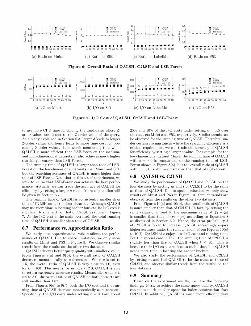
6.4 Overall RatioWe evaluate the overall ratio for 2-k-ANN search by vary-

ing k from 1 to 100. Results are shown in Figure 6.All the methods get satisfactory overall ratios, which are

much smaller than the theoretical bound c2 = 4. Com-pared to LSB-Forest, QALSH and C2LSH achieve signif-icantly higher accuracy. The overall ratios of QALSH andC2LSH are always smaller than 1.05, while the smallest over-all ratio of LSB-Forest on the four datasets is still larger than1.24. The overall ratios of QALSH are basically the sameas those of C2LSH. This is because the parameters whichaffect accuracy are set to be the same for both methods.

As k increases, the overall ratios of QALSH and C2LSHtend to increase while the overall ratio of LSB-Forest tendsto decrease. In fact, both QALSH and C2LSH return thebest k objects out of a candidate set of size βn+ k − 1. Ask increases, only k− 1 additional candidates are checked forpossible improvement on the ratios. In contrast, LSB-Foresttends to check relatively more objects.

6.5 I/O CostWe evaluate the I/O cost for 2-k-ANN search by varying

k from 1 to 100. The results6 are shown in Figure 7.Compared to QALSH and C2LSH, LSB-Forest requires

much smaller I/O costs on low- and medium-dimensionaldatasets, i.e., Mnist, Sift and LabelMe. However, its overallratio is much larger than those of QALSH and C2LSH. Forthe high-dimensional dataset P53, the I/O cost of QALSHis smaller than that of LSB-Forest. This is because the I/Ocost of LSB-Forest monotonically increases as data dimen-sionality d increases, while the I/O costs of QALSH andC2LSH are independent of d. Compared to C2LSH, QALSHuses about 49% to 76% of the I/O costs of C2LSH, but stillachieves the same accuracy.

When k increases, the I/O cost of LSB-Forest increasesgently, while the I/O costs of QALSH and C2LSH increasemore apparently. This is because LSB-Forest already storesthe coordinates of objects in each LSB-Tree, and hence itcomputes the Euclidean distance without extra I/O costs.However, neither QALSH nor C2LSH stores the coordinatesin hash tables, and thus one random I/O is needed for everycandidate in the worst case. As k increases, the number ofcandidates increases, and accordingly the I/O costs of bothQALSH and C2LSH increase.

6.6 Running TimeWe study the running time for 2-k-ANN search by varying

k from 1 to 100. The results are shown in Figure 8.Interestingly, the running time of LSB-Forest is larger

than that of QALSH on the medium-dimensional datasetLabelMe, even though its I/O cost is smaller than that ofQALSH. While the I/O cost of LSB-Forest is slightly largerthan that of QALSH on the high-dimensional dataset P53,the running time of LSB-Forest is surprisingly larger thanthat of QALSH by more than two orders of magnitude. Infact, as data dimensionality d increases, LSB-Forest tends

6I/O costs of brute-force linear scan method over thedatasets of Mnist, Sift, LabelMe and P53 are 3000, 125000,45249 and 10353, respectively.

9

1

1.2

1.4

1.6

1 10 20 30 40 50 60 70 80 90 100

Overa

ll R

ati

o

k

QALSH

C2LSH

LSB-Forest

(a) Ratio on Mnist

1

1.2

1.4

1.6

1 10 20 30 40 50 60 70 80 90 100

Overa

ll R

ati

o

k

QALSH

C2LSH

LSB-Forest

(b) Ratio on Sift

1

1.1

1.2

1.3

1.4

1.5

1 10 20 30 40 50 60 70 80 90 100

Overa

ll R

ati

o

k

QALSH

C2LSH

LSB-Forest

(c) Ratio on LabelMe

1

1.1

1.2

1.3

1.4

1 10 20 30 40 50 60 70 80 90 100

Overa

ll R

ati

o

k

QALSH

C2LSH

LSB-Forest

(d) Ratio on P53

Figure 6: Overall Ratio of QALSH, C2LSH and LSB-Forest

100

1000

10000

1 10 20 30 40 50 60 70 80 90 100

I/O

Cost

k

QALSH

C2LSH

LSB-Forest

(a) I/O on Mnist

1000

10000

100000

1 10 20 30 40 50 60 70 80 90 100

I/O

Cost

k

QALSH

C2LSH

LSB-Forest

(b) I/O on Sift

0

2000

4000

6000

1 10 20 30 40 50 60 70 80 90 100

I/O

Cost

k

QALSH

C2LSH

LSB-Forest

(c) I/O on LabelMe

0

300

600

900

1 10 20 30 40 50 60 70 80 90 100

I/O

Cost

k

QALSH

C2LSH

LSB-Forest

(d) I/O on P53

Figure 7: I/O Cost of QALSH, C2LSH and LSB-Forest

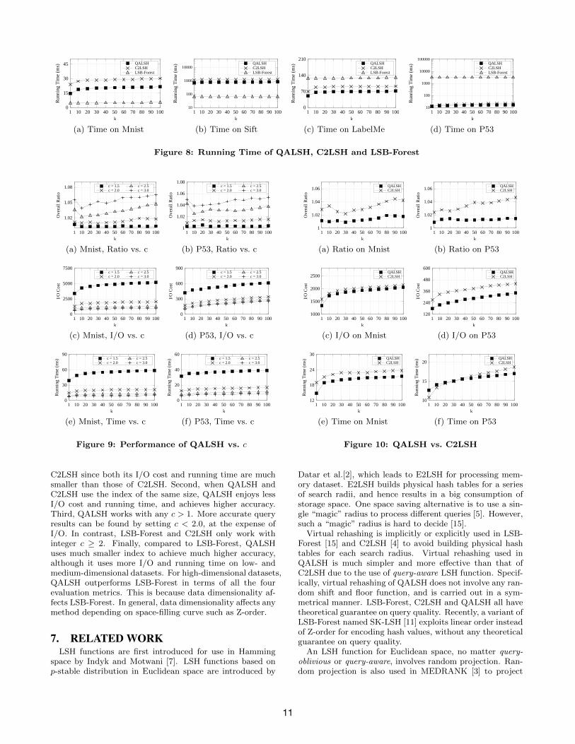
to use more CPU time for finding the candidates whose Z-order values are closest to the Z-order value of the query.As already explained in Section 6.3, larger d leads to longerZ-order values and hence leads to more time cost for pro-cessing Z-order values. It is worth mentioning that whileQALSH is more efficient than LSB-forest on the medium-and high-dimensional datasets, it also achieves much highersearching accuracy than LSB-Forest.

The running time of QALSH is larger than that of LSB-Forest on the low-dimensional datasets, i.e., Mnist and Sift,but the searching accuracy of QALSH is much higher thanthat of LSB-Forest. Note that in this set of experiments, weset c to 2.0 so that LSB-Forest can achieve the best perfor-mance. Actually, we can trade the accuracy of QALSH forefficiency by setting a larger c value. More explanation willbe given in Section 6.7.

The running time of QALSH is consistently smaller thanthat of C2LSH on all the four datasets. Although QALSHmay use more time in locating anchor buckets, its I/O cost issignificantly smaller than that of C2LSH as shown in Figure7. As the I/O cost is the main overhead, the total runningtime of QALSH is smaller than that of C2LSH.

6.7 Performance vs. Approximation RatioWe study how approximation ratio c affects the perfor-

mance of QALSH. Due to space limitation, we only showresults on Mnist and P53 in Figure 9. We observe similartrends from the results on the other two datasets.

QALSH achieves better query quality with smaller c value.From Figures 9(a) and 9(b), the overall ratio of QALSHdecreases monotonically as c decreases. When c is set to1.5, the overall ratio of QALSH is very close to 1.0, evenfor k = 100. This means, by using c < 2.0, QALSH is ableto return extremely accurate results. Meanwhile, when c isset to 3.0, the overall ratios of QALSH on both datasets arestill smaller than 1.07.

From Figures 9(c) to 9(f), both the I/O cost and the run-ning time of QALSH decrease monotonically as c increases.Specifically, the I/O costs under setting c = 3.0 are about

25% and 50% of the I/O costs under setting c = 1.5 overthe datasets Mnist and P53, respectively. Similar trends canbe observed for the running time of QALSH. Therefore, un-der certain circumstances where the searching efficiency is acritical requirement, we can trade the accuracy of QALSHfor efficiency by setting a larger c value. For example, for thelow-dimensional dataset Mnist, the running time of QALSHwith c = 3.0 is comparable to the running time of LSB-Forest shown in Figure 8(a), but the overall ratio of QALSHwith c = 3.0 is still much smaller than that of LSB-Forest.

6.8 QALSH vs. C2LSHWe study the performance of QALSH and C2LSH on the

four datasets by setting m and l of C2LSH to be the sameas those of QALSH. Due to space limitation, we only showresults on Mnist and P53 in Figure 10. Similar trends areobserved from the results on the other two datasets.

From Figures 10(a) and 10(b), the overall ratio of QALSHis much smaller than that of C2LSH. In fact, by setting thesame values of m and β, the maximum value of (ξ1 − ξ2)is smaller than that of (p1 − p2) according to Equation 8as discussed in Section 3.2. Hence, the error probability δof C2LSH is forced to increase. QALSH accordingly enjoyshigher accuracy under the same m and l. From Figures 10(c)to 10(f), QALSH also enjoys less I/O cost and running time.For the special case in P53, the running time of C2LSH isslightly less than that of QALSH when k ≤ 30. This isbecause their I/O costs are close to each other, but QALSHneeds more time in locating the anchor buckets.

We also study the performance of QALSH and C2LSHby setting m and l of QALSH to be the same as those ofC2LSH, and observe similar trends from the results on thefour datasets.

6.9 SummaryBased on the experiment results, we have the following

findings. First, to achieve the same query quality, QALSHconsumes much smaller space for index construction thanC2LSH. In addition, QALSH is much more efficient than

10

0

15

30

45

1 10 20 30 40 50 60 70 80 90 100

Runnin

g T

ime

(ms)

k

QALSHC2LSHLSB-Forest

(a) Time on Mnist

10

100

1000

10000

1 10 20 30 40 50 60 70 80 90 100

Runnin

g T

ime

(ms)

k

QALSHC2LSHLSB-Forest

(b) Time on Sift

0

70

140

210

1 10 20 30 40 50 60 70 80 90 100

Runnin

g T

ime

(ms)

k

QALSHC2LSHLSB-Forest

(c) Time on LabelMe

10

100

1000

10000

100000

1 10 20 30 40 50 60 70 80 90 100

Runnin

g T

ime

(ms)

k

QALSHC2LSHLSB-Forest

(d) Time on P53

Figure 8: Running Time of QALSH, C2LSH and LSB-Forest

1.02

1.05

1.08

1 10 20 30 40 50 60 70 80 90 100

Overa

ll R

ati

o

k

c = 1.5

c = 2.0

c = 2.5

c = 3.0

(a) Mnist, Ratio vs. c

1

1.02

1.04

1.06

1.08

1 10 20 30 40 50 60 70 80 90 100

Overa

ll R

ati

o

k

c = 1.5

c = 2.0

c = 2.5

c = 3.0

(b) P53, Ratio vs. c

0

2500

5000

7500

1 10 20 30 40 50 60 70 80 90 100

I/O

Cost

k

c = 1.5

c = 2.0

c = 2.5

c = 3.0

(c) Mnist, I/O vs. c

0

300

600

900

1 10 20 30 40 50 60 70 80 90 100

I/O

Cost

k

c = 1.5

c = 2.0

c = 2.5

c = 3.0

(d) P53, I/O vs. c

0

30

60

90

1 10 20 30 40 50 60 70 80 90 100

Runnin

g T

ime

(ms)

k

c = 1.5c = 2.0

c = 2.5c = 3.0

(e) Mnist, Time vs. c

0

20

40

60

1 10 20 30 40 50 60 70 80 90 100

Runnin

g T

ime

(ms)

k

c = 1.5c = 2.0

c = 2.5c = 3.0

(f) P53, Time vs. c

Figure 9: Performance of QALSH vs. c

C2LSH since both its I/O cost and running time are muchsmaller than those of C2LSH. Second, when QALSH andC2LSH use the index of the same size, QALSH enjoys lessI/O cost and running time, and achieves higher accuracy.Third, QALSH works with any c > 1. More accurate queryresults can be found by setting c < 2.0, at the expense ofI/O. In contrast, LSB-Forest and C2LSH only work withinteger c ≥ 2. Finally, compared to LSB-Forest, QALSHuses much smaller index to achieve much higher accuracy,although it uses more I/O and running time on low- andmedium-dimensional datasets. For high-dimensional datasets,QALSH outperforms LSB-Forest in terms of all the fourevaluation metrics. This is because data dimensionality af-fects LSB-Forest. In general, data dimensionality affects anymethod depending on space-filling curve such as Z-order.

7. RELATED WORKLSH functions are first introduced for use in Hamming

space by Indyk and Motwani [7]. LSH functions based onp-stable distribution in Euclidean space are introduced by

1

1.02

1.04

1.06

1 10 20 30 40 50 60 70 80 90 100

Overa

ll R

ati

o

k

QALSH

C2LSH

(a) Ratio on Mnist

1

1.02

1.04

1.06

1 10 20 30 40 50 60 70 80 90 100

Overa

ll R

ati

o

k

QALSH

C2LSH

(b) Ratio on P53

1000

1500

2000

2500

1 10 20 30 40 50 60 70 80 90 100

I/O

Cost

k

QALSH

C2LSH

(c) I/O on Mnist

120

240

360

480

600

1 10 20 30 40 50 60 70 80 90 100

I/O

Cost

k

QALSH

C2LSH

(d) I/O on P53

12

18

24

30

1 10 20 30 40 50 60 70 80 90 100

Runnin

g T

ime

(ms)

k

QALSHC2LSH

(e) Time on Mnist

10

15

20

1 10 20 30 40 50 60 70 80 90 100

Runnin

g T

ime

(ms)

k

QALSHC2LSH

(f) Time on P53

Figure 10: QALSH vs. C2LSH

Datar et al.[2], which leads to E2LSH for processing mem-ory dataset. E2LSH builds physical hash tables for a seriesof search radii, and hence results in a big consumption ofstorage space. One space saving alternative is to use a sin-gle “magic” radius to process different queries [5]. However,such a “magic” radius is hard to decide [15].

Virtual rehashing is implicitly or explicitly used in LSB-Forest [15] and C2LSH [4] to avoid building physical hashtables for each search radius. Virtual rehashing used inQALSH is much simpler and more effective than that ofC2LSH due to the use of query-aware LSH function. Specif-ically, virtual rehashing of QALSH does not involve any ran-dom shift and floor function, and is carried out in a sym-metrical manner. LSB-Forest, C2LSH and QALSH all havetheoretical guarantee on query quality. Recently, a variant ofLSB-Forest named SK-LSH [11] exploits linear order insteadof Z-order for encoding hash values, without any theoreticalguarantee on query quality.

An LSH function for Euclidean space, no matter query-oblivious or query-aware, involves random projection. Ran-dom projection is also used in MEDRANK [3] to project

11

objects over a set of m random lines. However, MEDRANKdoes not segment a random line into buckets. An objectthat is found closest to a query along at least m

2random

lines, is reported as the c-ANN of the query. The medianthreshold of m

2is generalized by collision threshold for find-

ing frequent objects in both C2LSH and QALSH. A clas-sic result on random projection is the Johnson-LindenstrassLemma [9], which states that by projecting objects in d-dimensional Euclidean space along m random lines, the dis-tance in the original d-dimensions can be approximately pre-served in the m-dimensions. In a recent work on LSH formemory dataset in Euclidean space, Andoni et al.[1] proposeto replace random projection (i.e., data-oblivious projection)by data-aware projection. However, the LSH scheme is stillquery-oblivious. Recently, Sun et al.[14] introduce anotherprojection-based method named SRS. SRS uses only 6 ran-dom projections to convert high-dimensional data objectsinto low-dimensional ones so that they can be indexed bya single R-tree. While C2LSH has better overall ratio thanSRS, SRS uses a rather small index and also incurs muchless I/O cost. Since SRS exploits only 6 to 10 random pro-jections, it is natural to expect one is able to perform severalgroups of such projections. However, it is not clear whichgroup of projections in SRS would lead to the best over-all ratio. Intuitively, SRS is less stable than C2LSH andQALSH, since SRS is based on less than 10 projections butC2LSH and QALSH take advantage of more projections.

8. CONCLUSIONSIn this paper, we introduce a novel concept of query-aware

LSH function and accordingly propose a novel LSH schemeQALSH for c-ANN search in high-dimensional Euclideanspace. A query-aware LSH function is a random projectioncoupled with query-aware bucket partition. The functionneeds no random shift that is a prerequisite of traditionalLSH functions. Query-aware LSH functions also enablesQALSH to work with any approximation ratio c > 1. Incontrast, the state-of-the-art LSH schemes such as C2LSHand LSB-Forest only work with integer c ≥ 2. Our theoret-ical analysis shows that QALSH achieves a quality guaran-tee for the c-ANN search. We also propose an automaticway to decide the bucket width w used in QALSH. Ex-perimental results on four real datasets demonstrate thatQALSH outperforms C2LSH and LSB-Forest, especially inhigh-dimensional space.

9. ACKNOWLEDGMENTSThis work is partially supported by China NSF Grant

60970043, HKUST FSGRF13EG22 and FSGRF14EG31. Wethank Wei Wang (UNSW) for his insightful comments.

10. REFERENCES[1] A. Andoni, P. Indyk, H. L. Nguyen, and

I. Razenshteyn. Beyond locality-sensitive hashing. InSODA, pages 1018–1028, 2014.

[2] M. Datar, N. Immorlica, P. Indyk, and V. S. Mirrokni.Locality-sensitive hashing scheme based on p-stabledistributions. In SoCG, pages 253–262, 2004.

[3] R. Fagin, R. Kumar, and D. Sivakumar. Efficientsimilarity search and classification via rankaggregation. In ACM SIGMOD, pages 301–312, 2003.

[4] J. Gan, J. Feng, Q. Fang, and W. Ng.Locality-sensitive hashing scheme based on dynamiccollision counting. In SIGMOD, pages 541–552, 2012.

[5] A. Gionis, P. Indyk, R. Motwani, et al. Similaritysearch in high dimensions via hashing. In VLDB,volume 99, pages 518–529. VLDB Endowment, 1999.

[6] W. Hoeffding. Probability inequalities for sums ofbounded random variables. Journal of the AmericanStatistical Association, 58(301):13–30, 1963.

[7] P. Indyk and R. Motwani. Approximate nearestneighbors: towards removing the curse ofdimensionality. In ACM STOC, pages 604–613, 1998.

[8] H. Jagadish, B. C. Ooi, K.-L. Tan, C. Yu, andR. Zhang. idistance: an adaptive b+-tree basedindexing method for nearest neighbor search. ACMTODS, 30(2):364–397, 2005.

[9] W. Johnson and J. Lindenstrauss. Extensions oflipshitz mapping into hilbert space. ContemporaryMathematics, 26:189–206, 1984.

[10] J. M. Kleinberg. Two algorithms for nearest-neighborsearch in high dimensions. In ACM STOC, pages599–608, 1997.

[11] Y. Liu, J. Cui, Z. Huang, H. Li, and H. T. Shen.Sk-lsh: An efficient index structure for approximatenearest neighbor search. VLDB, 7(9), 2014.

[12] R. Panigrahy. Entropy based nearest neighbor searchin high dimensions. In ACM-SIAM SODA, pages1186–1195, 2006.

[13] H. Samet. Foundations of multidimensional andmetric data structures. Morgan Kaufmann, 2006.

[14] Y. Sun, W. Wang, J. Qin, Y. Zhang, and X. Lin. Srs:Solving c-approximate nearest neighbor queries inhigh dimensional euclidean space with a tiny index.VLDB, 8(1), 2014.

[15] Y. Tao, K. Yi, C. Sheng, and P. Kalnis. Efficient andaccurate nearest neighbor and closest pair search inhigh-dimensional space. ACM TODS, 35(3):20, 2010.

APPENDIXA. PROOF OF LEMMA 3

Proof. Before bounding Pr[P1 ∩ P2] from below andhence proving Lemma 3, we have to prove lower boundson P1 and P2.

We now show some details of proving Pr[P1] ≥ 1 − δ.Let S1 = {o | ‖o− q‖ ≤ R}. For ∀o ∈ S1, Pr[P1] =Pr[#Col(o) ≥ αm] =

∑mi=dαme C

imp

i(1− p)m−i, where p =

Pr[|HR~aj

(o) −HR~aj

(q)| ≤ w2

] ≥ p1 > α, j = 1, 2, ...,m. Then

by following the same reasoning based on Hoeffding’s In-equality [6] from Lemma 1 of C2LSH, we have Pr[P1] ≥1− δ, when m =

⌈max

(1

2(p1−α)2ln 1

δ, 12(α−p2)2

ln 2β

)⌉.

Similarly, using the same m, we have Pr[P2] > 12.

For the (R, c)-NN search, since QALSH terminates wheneither P1 or P2 holds, we have Pr[P1∪P2] = 1. We also havethe formula: Pr[P1 ∪P2] = Pr[P1] + Pr[P2]− Pr[P1 ∩P2].Therefore, we can bound Pr[P1∩P2] from below as follows:

Pr[P1 ∩ P2] = Pr[P1] + Pr[P2]− Pr[P1 ∪ P2]≥ 1− δ + 1

2− 1 = 1

2− δ

And hence Lemma 3 is proved.

12