Query Optimization

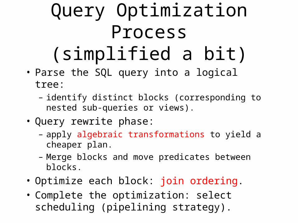
Query Optimization Process(simplified a bit)

• Parse the SQL query into a logical tree:– identify distinct blocks (corresponding to nested sub-

queries or views).

• Query rewrite phase:– apply algebraic transformations to yield a cheaper plan.

– Merge blocks and move predicates between blocks.

• Optimize each block: join ordering.• Complete the optimization: select scheduling

(pipelining strategy).

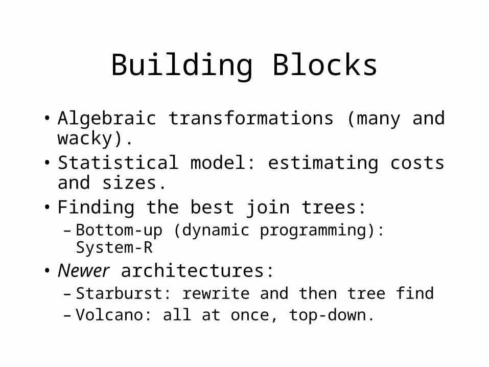
Building Blocks

• Algebraic transformations (many and wacky).

• Statistical model: estimating costs and sizes.• Finding the best join trees:

– Bottom-up (dynamic programming): System-R

• Newer architectures:– Starburst: rewrite and then tree find– Volcano: all at once, top-down.

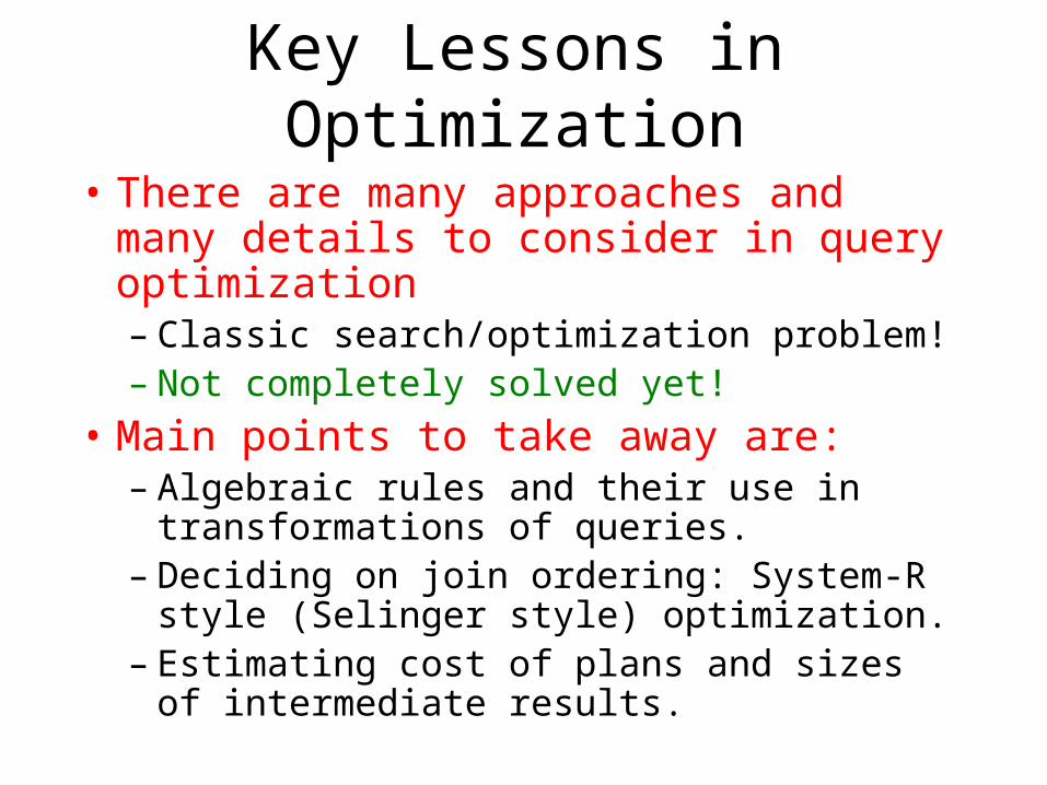
Key Lessons in Optimization

• There are many approaches and many details to consider in query optimization– Classic search/optimization problem!– Not completely solved yet!

• Main points to take away are:– Algebraic rules and their use in transformations

of queries.– Deciding on join ordering: System-R style

(Selinger style) optimization.– Estimating cost of plans and sizes of

intermediate results.

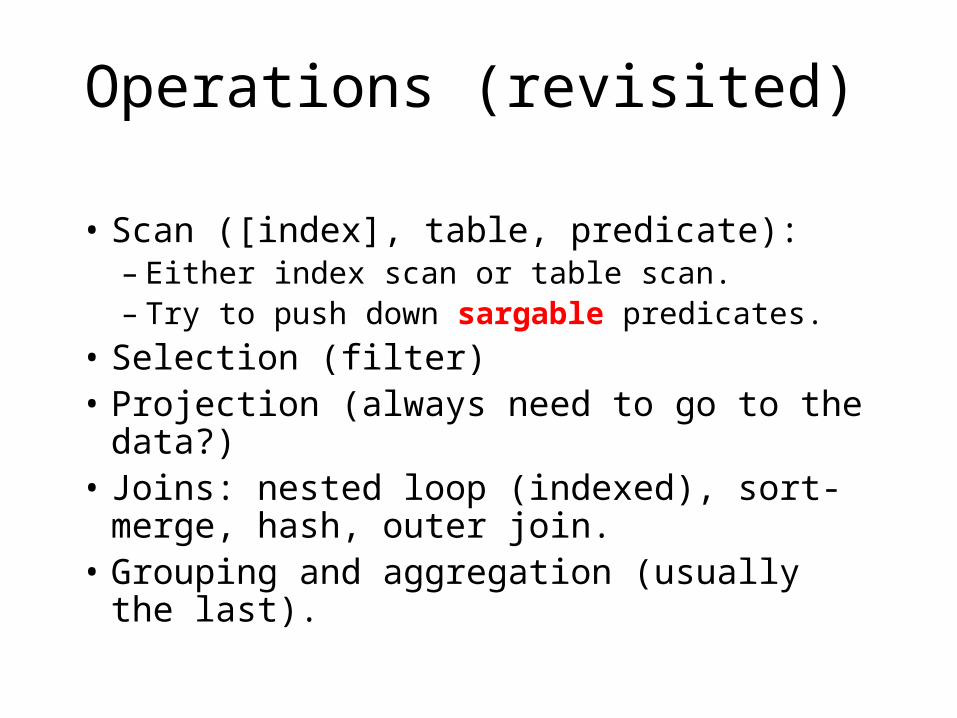
Operations (revisited)

• Scan ([index], table, predicate):– Either index scan or table scan.– Try to push down sargable predicates.

• Selection (filter)• Projection (always need to go to the data?)• Joins: nested loop (indexed), sort-merge,

hash, outer join.• Grouping and aggregation (usually the last).

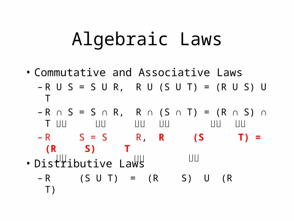
Algebraic Laws

• Commutative and Associative Laws– R U S = S U R, R U (S U T) = (R U S) U T– R ∩ S = S ∩ R, R ∩ (S ∩ T) = (R ∩ S) ∩ T– R S = S R, R (S T) = (R S) T

• Distributive Laws– R (S U T) = (R S) U (R T)

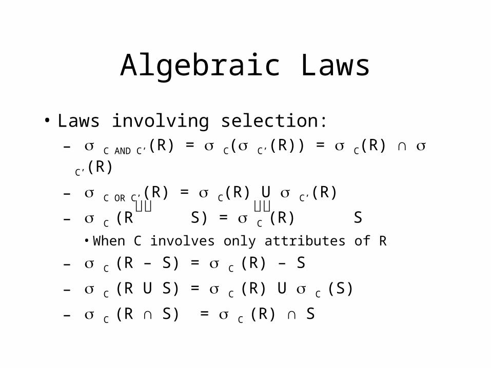
Algebraic Laws

• Laws involving selection:– C AND C’(R) = C( C’(R)) = C(R) ∩ C’(R)

– C OR C’(R) = C(R) U C’(R)

– C (R S) = C (R) S • When C involves only attributes of R

– C (R – S) = C (R) – S

– C (R U S) = C (R) U C (S)

– C (R ∩ S) = C (R) ∩ S

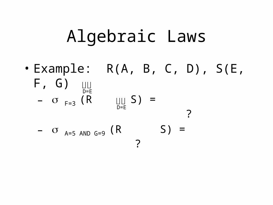
Algebraic Laws

• Example: R(A, B, C, D), S(E, F, G)– F=3 (R S) = ?

– A=5 AND G=9 (R S) = ?

D=E

D=E

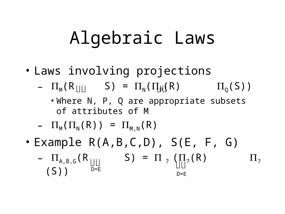
Algebraic Laws

• Laws involving projections– M(R S) = N(P(R) Q(S))

• Where N, P, Q are appropriate subsets of attributes of M

– M(N(R)) = M,N(R)

• Example R(A,B,C,D), S(E, F, G)– A,B,G(R S) = ? (?(R) ?(S))

D=ED=E

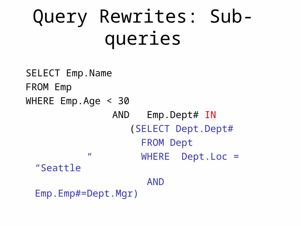
Query Rewrites: Sub-queries

SELECT Emp.Name

FROM Emp

WHERE Emp.Age < 30

AND Emp.Dept# IN

(SELECT Dept.Dept#

FROM Dept

WHERE Dept.Loc = “Seattle”

AND Emp.Emp#=Dept.Mgr)

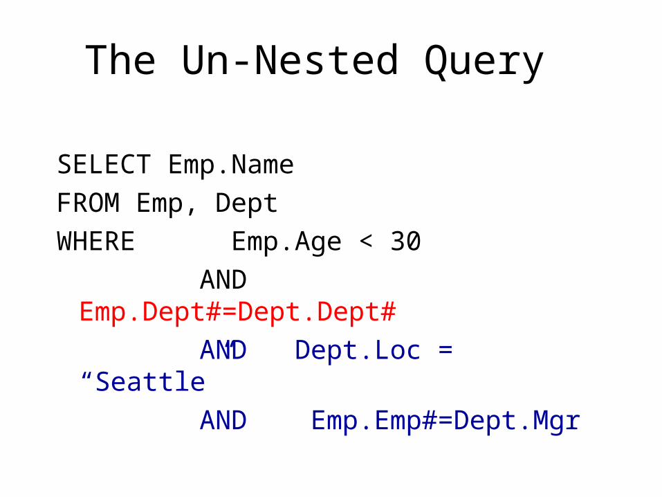
The Un-Nested Query

SELECT Emp.Name

FROM Emp, Dept

WHERE Emp.Age < 30

AND Emp.Dept#=Dept.Dept#

AND Dept.Loc = “Seattle”

AND Emp.Emp#=Dept.Mgr

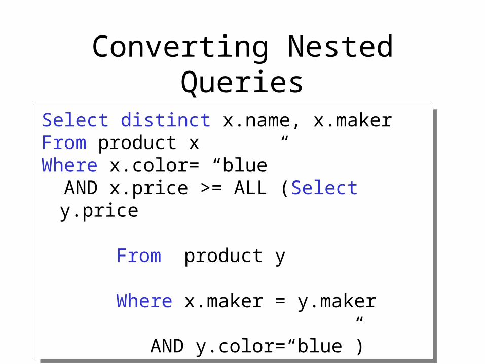
Converting Nested Queries

Select distinct x.name, x.makerFrom product xWhere x.color= “blue” AND x.price >= ALL (Select y.price From product y Where x.maker = y.maker AND y.color=“blue”)

Select distinct x.name, x.makerFrom product xWhere x.color= “blue” AND x.price >= ALL (Select y.price From product y Where x.maker = y.maker AND y.color=“blue”)

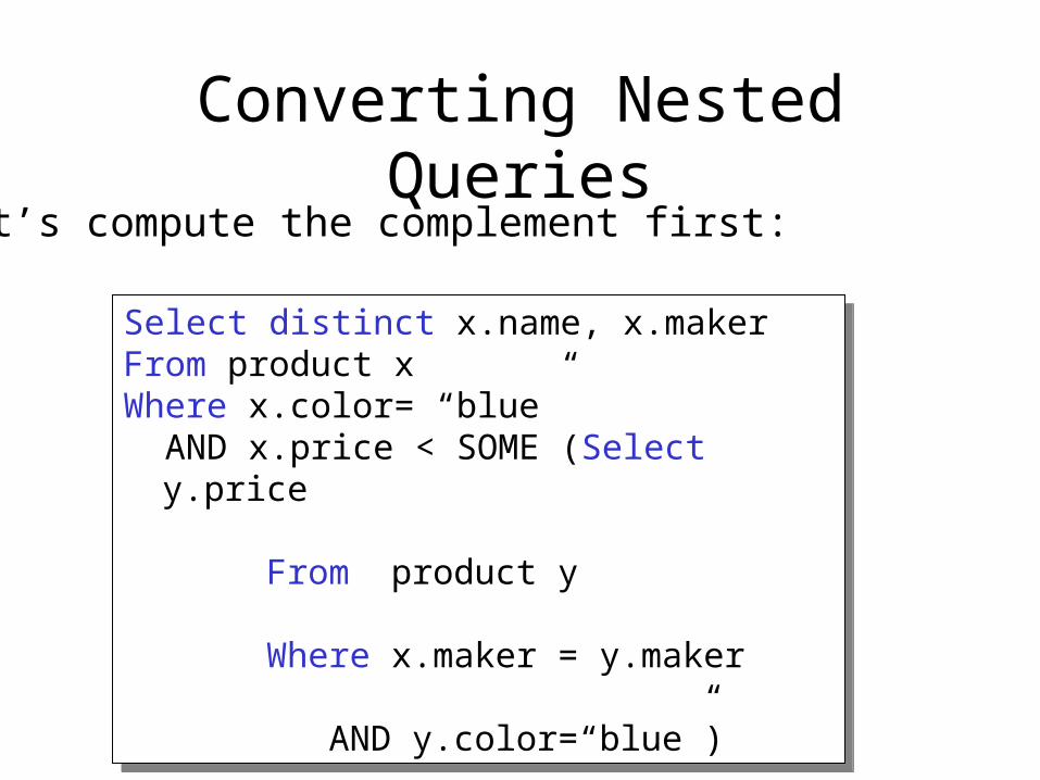
Converting Nested Queries

Select distinct x.name, x.makerFrom product xWhere x.color= “blue” AND x.price < SOME (Select y.price From product y Where x.maker = y.maker AND y.color=“blue”)

Select distinct x.name, x.makerFrom product xWhere x.color= “blue” AND x.price < SOME (Select y.price From product y Where x.maker = y.maker AND y.color=“blue”)

Let’s compute the complement first:

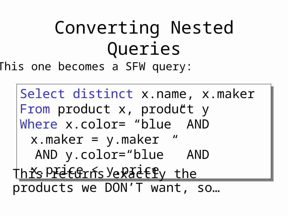
Converting Nested Queries

Select distinct x.name, x.makerFrom product x, product yWhere x.color= “blue” AND x.maker =

y.maker AND y.color=“blue” AND x.price < y.price

Select distinct x.name, x.makerFrom product x, product yWhere x.color= “blue” AND x.maker =

y.maker AND y.color=“blue” AND x.price < y.price

This one becomes a SFW query:

This returns exactly the products we DON’T want, so…

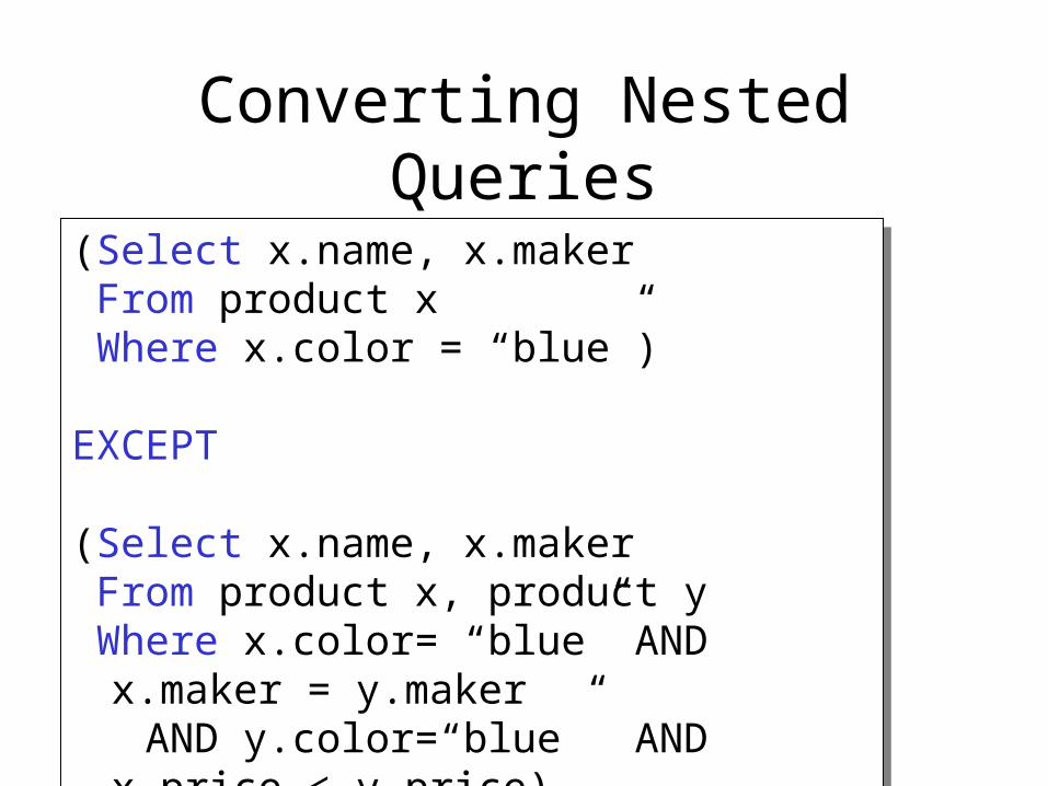
Converting Nested Queries

(Select x.name, x.maker From product x Where x.color = “blue”)

EXCEPT

(Select x.name, x.maker From product x, product y Where x.color= “blue” AND x.maker = y.maker AND y.color=“blue” AND x.price < y.price)

(Select x.name, x.maker From product x Where x.color = “blue”)

EXCEPT

(Select x.name, x.maker From product x, product y Where x.color= “blue” AND x.maker = y.maker AND y.color=“blue” AND x.price < y.price)

Semi-Joins, Magic Sets

Semi-Joins, Magic Sets

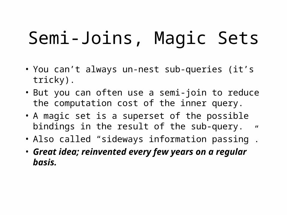
• You can’t always un-nest sub-queries (it’s tricky).• But you can often use a semi-join to reduce the

computation cost of the inner query.• A magic set is a superset of the possible bindings

in the result of the sub-query.• Also called “sideways information passing”.• Great idea; reinvented every few years on a

regular basis.

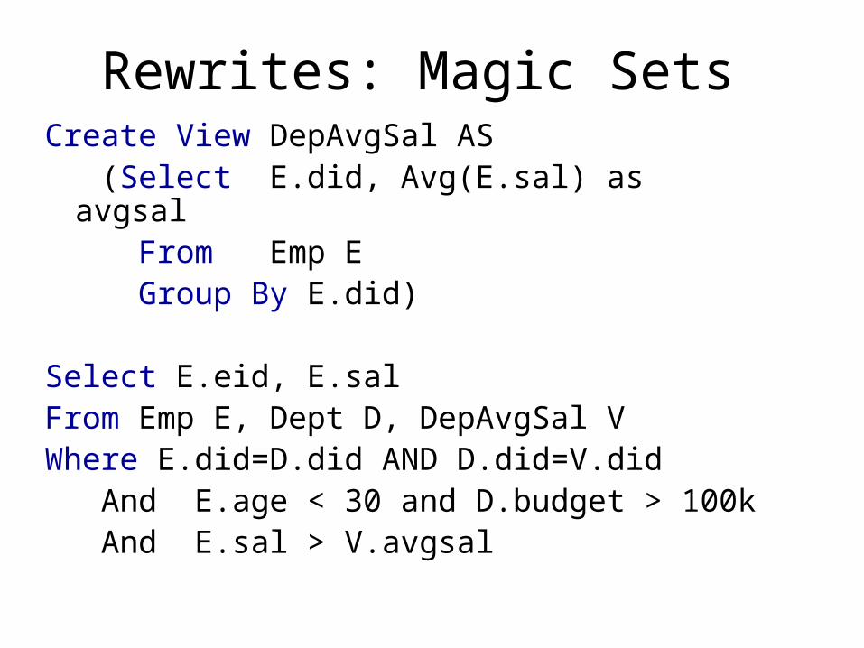
Rewrites: Magic SetsCreate View DepAvgSal AS (Select E.did, Avg(E.sal) as avgsal From Emp E Group By E.did)

Select E.eid, E.salFrom Emp E, Dept D, DepAvgSal VWhere E.did=D.did AND D.did=V.did And E.age < 30 and D.budget > 100k And E.sal > V.avgsal

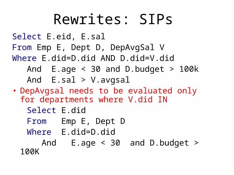
Rewrites: SIPsSelect E.eid, E.salFrom Emp E, Dept D, DepAvgSal VWhere E.did=D.did AND D.did=V.did And E.age < 30 and D.budget > 100k And E.sal > V.avgsal• DepAvgsal needs to be evaluated only for

departments where V.did IN Select E.did From Emp E, Dept D Where E.did=D.did And E.age < 30 and D.budget > 100K

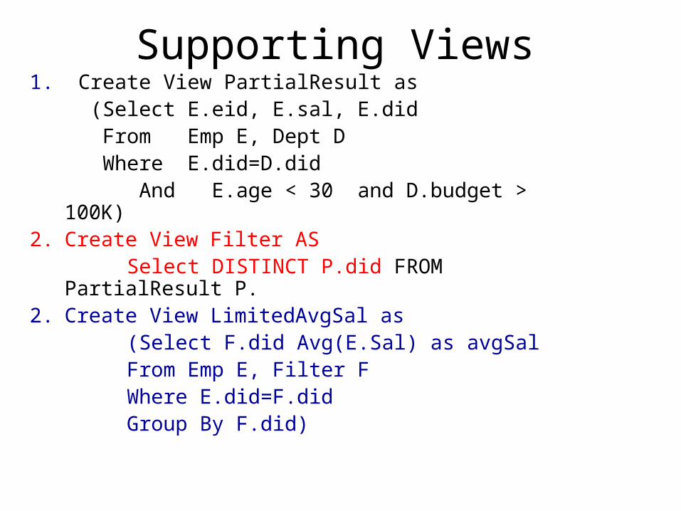
Supporting Views1. Create View PartialResult as (Select E.eid, E.sal, E.did From Emp E, Dept D Where E.did=D.did And E.age < 30 and D.budget > 100K)2. Create View Filter AS Select DISTINCT P.did FROM PartialResult P.2. Create View LimitedAvgSal as (Select F.did Avg(E.Sal) as avgSal From Emp E, Filter F Where E.did=F.did Group By F.did)

And Finally…

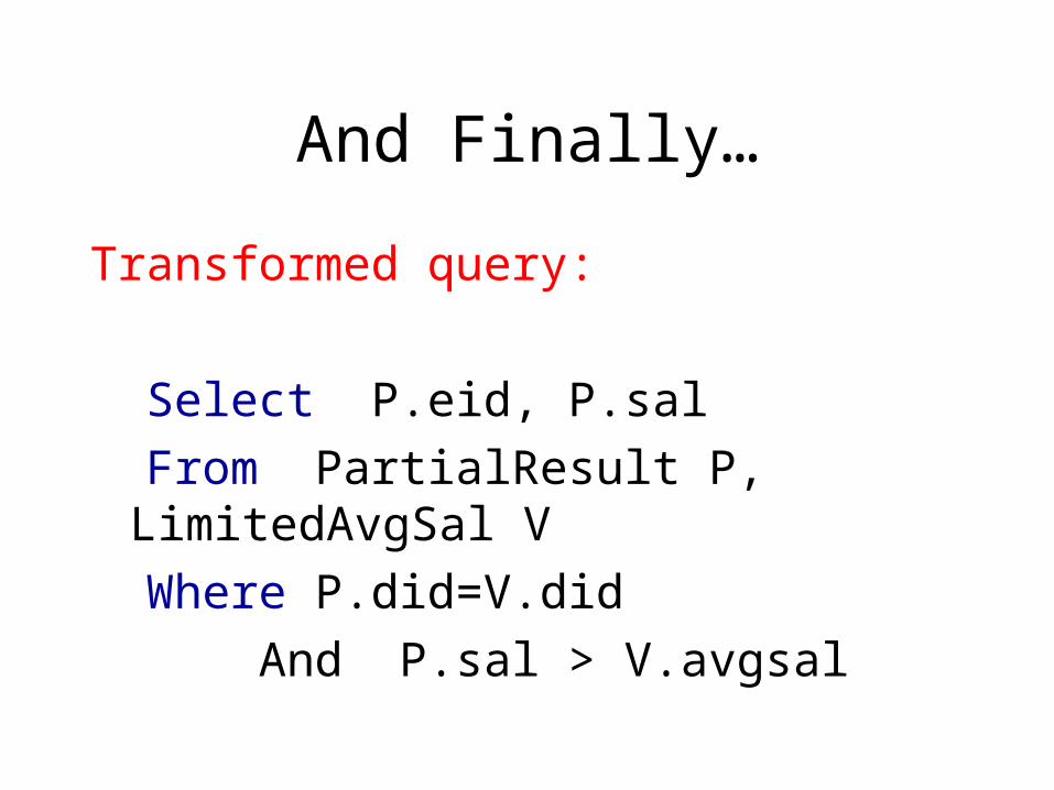
Transformed query:

Select P.eid, P.sal

From PartialResult P, LimitedAvgSal V

Where P.did=V.did

And P.sal > V.avgsal

Rewrites: Group By and Join

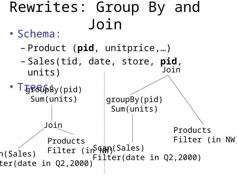
Rewrites: Group By and Join• Schema:

– Product (pid, unitprice,…)– Sales(tid, date, store, pid, units)

• Trees:

Join

groupBy(pid)Sum(units)

Scan(Sales)Filter(date in Q2,2000)

ProductsFilter (in NW)

Join

groupBy(pid)Sum(units)

Scan(Sales)Filter(date in Q2,2000)

ProductsFilter (in NW)

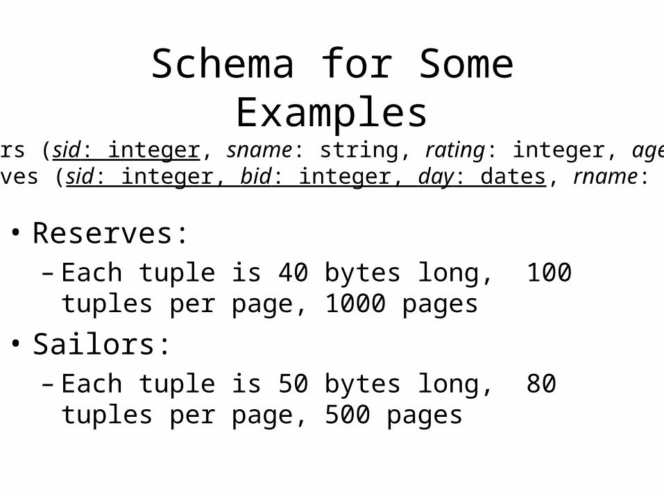
Schema for Some Examples

• Reserves:– Each tuple is 40 bytes long, 100 tuples per page, 1000

pages

• Sailors:– Each tuple is 50 bytes long, 80 tuples per page, 500

pages

Sailors (sid: integer, sname: string, rating: integer, age: real)Reserves (sid: integer, bid: integer, day: dates, rname: string)

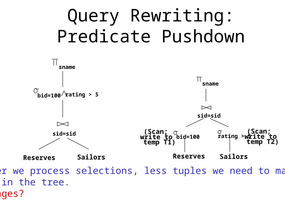
Query Rewriting: Predicate Pushdown

Reserves Sailors

sid=sid

bid=100 rating > 5

sname

Reserves Sailors

sid=sid

bid=100

sname

rating > 5(Scan;write to temp T1)

(Scan;write totemp T2)

The earlier we process selections, less tuples we need to manipulatehigher up in the tree.Disadvantages?

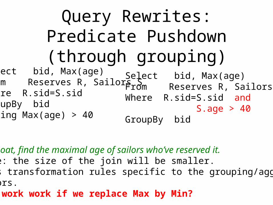
Query Rewrites: Predicate Pushdown (through grouping)

Select bid, Max(age)From Reserves R, Sailors SWhere R.sid=S.sid GroupBy bidHaving Max(age) > 40

Select bid, Max(age)From Reserves R, Sailors SWhere R.sid=S.sid and S.age > 40GroupBy bid

• For each boat, find the maximal age of sailors who’ve reserved it.•Advantage: the size of the join will be smaller.• Requires transformation rules specific to the grouping/aggregation operators.• Will it work work if we replace Max by Min?

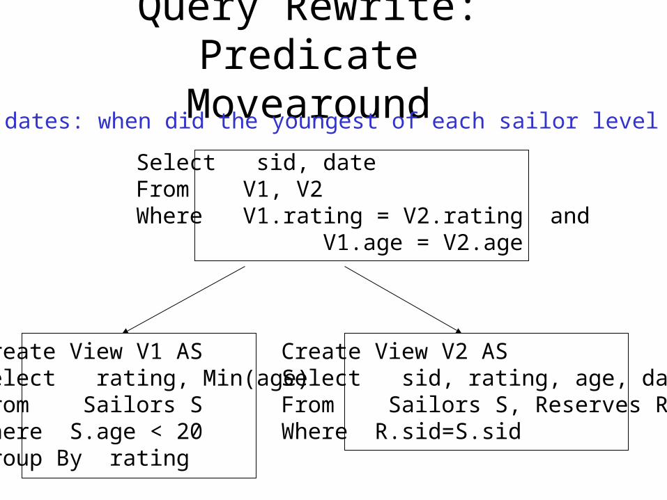
Query Rewrite:Predicate Movearound

Create View V1 ASSelect rating, Min(age)From Sailors SWhere S.age < 20Group By rating

Create View V2 ASSelect sid, rating, age, dateFrom Sailors S, Reserves RWhere R.sid=S.sid

Select sid, dateFrom V1, V2Where V1.rating = V2.rating and V1.age = V2.age

Sailing wiz dates: when did the youngest of each sailor level rent boats?

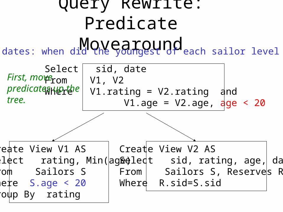
Query Rewrite: Predicate Movearound

Create View V1 ASSelect rating, Min(age)From Sailors SWhere S.age < 20Group By rating

Create View V2 ASSelect sid, rating, age, dateFrom Sailors S, Reserves RWhere R.sid=S.sid

Select sid, dateFrom V1, V2Where V1.rating = V2.rating and V1.age = V2.age, age < 20

Sailing wiz dates: when did the youngest of each sailor level rent boats?

First, move predicates up the tree.

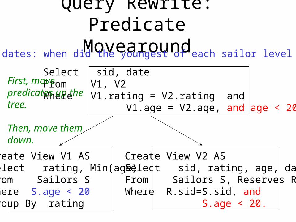
Query Rewrite: Predicate Movearound

Create View V1 ASSelect rating, Min(age)From Sailors SWhere S.age < 20Group By rating

Create View V2 ASSelect sid, rating, age, dateFrom Sailors S, Reserves RWhere R.sid=S.sid, and S.age < 20.

Select sid, dateFrom V1, V2Where V1.rating = V2.rating and V1.age = V2.age, and age < 20

Sailing wiz dates: when did the youngest of each sailor level rent boats?

First, move predicates up the tree.

Then, move themdown.

Query Rewrite Summary• The optimizer can use any semantically correct

rule to transform one query to another.• Rules try to:

– move constraints between blocks (because each will be optimized separately)

– Unnest blocks

• Especially important in decision support applications where queries are very complex.

• In a few minutes of thought, you’ll come up with your own rewrite. Some query, somewhere, will benefit from it.

• Theorems?

Cost Estimation

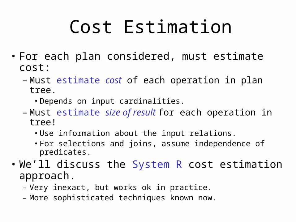
• For each plan considered, must estimate cost:– Must estimate cost of each operation in plan tree.

• Depends on input cardinalities.

– Must estimate size of result for each operation in tree!• Use information about the input relations.• For selections and joins, assume independence of predicates.

• We’ll discuss the System R cost estimation approach.– Very inexact, but works ok in practice.– More sophisticated techniques known now.

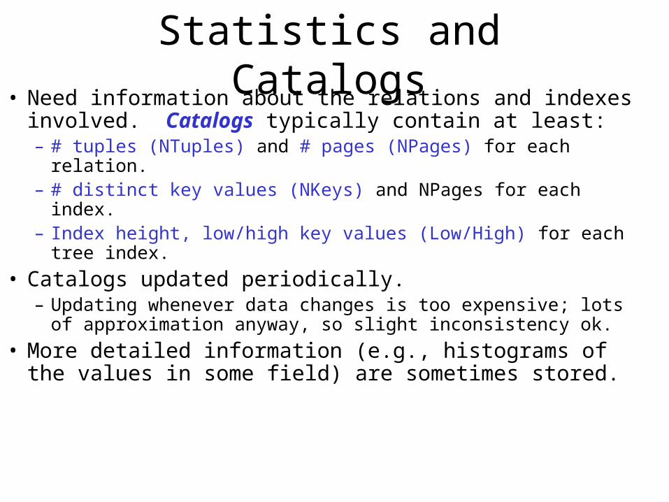
Statistics and Catalogs• Need information about the relations and indexes

involved. Catalogs typically contain at least:– # tuples (NTuples) and # pages (NPages) for each relation.– # distinct key values (NKeys) and NPages for each index.– Index height, low/high key values (Low/High) for each tree

index.

• Catalogs updated periodically.– Updating whenever data changes is too expensive; lots of

approximation anyway, so slight inconsistency ok.

• More detailed information (e.g., histograms of the values in some field) are sometimes stored.

Size Estimation and Reduction Factors

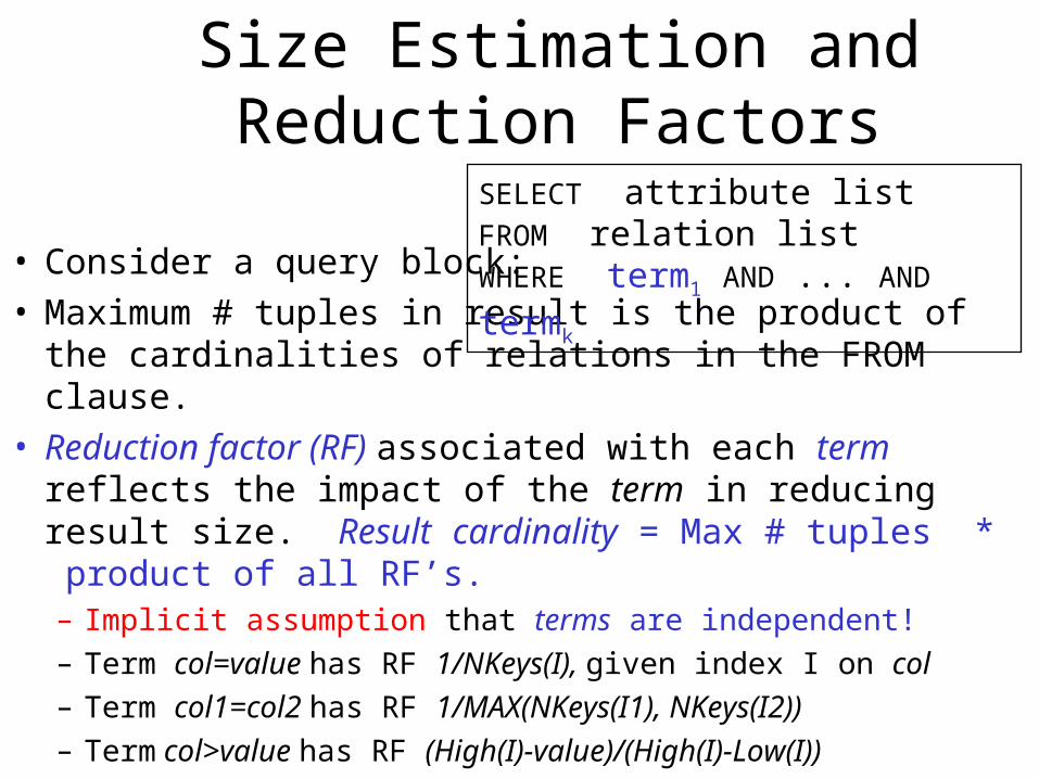
• Consider a query block:• Maximum # tuples in result is the product of the

cardinalities of relations in the FROM clause.• Reduction factor (RF) associated with each term reflects

the impact of the term in reducing result size. Result cardinality = Max # tuples * product of all RF’s.– Implicit assumption that terms are independent!

– Term col=value has RF 1/NKeys(I), given index I on col

– Term col1=col2 has RF 1/MAX(NKeys(I1), NKeys(I2))

– Term col>value has RF (High(I)-value)/(High(I)-Low(I))

SELECT attribute listFROM relation listWHERE term1 AND ... AND termk

Histograms

• Key to obtaining good cost and size estimates.

• Come in several flavors:– Equi-depth– Equi-width

• Which is better?• Compressed histograms: special treatment

of frequent values.

Histograms

• Statistics on data maintained by the RDBMS

• Makes size estimation much more accurate (hence, cost estimations are more accurate)

Histograms

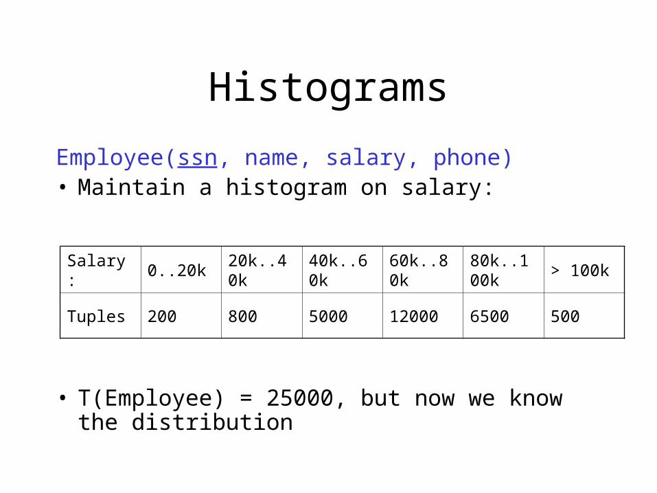
Employee(ssn, name, salary, phone)• Maintain a histogram on salary:

• T(Employee) = 25000, but now we know the distribution

Salary: 0..20k 20k..40k 40k..60k 60k..80k 80k..100k > 100k

Tuples 200 800 5000 12000 6500 500

Histograms

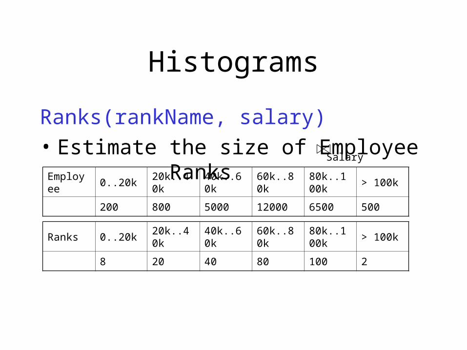
Ranks(rankName, salary)

• Estimate the size of Employee RanksEmployee 0..20k 20k..40k 40k..60k 60k..80k 80k..100k > 100k

200 800 5000 12000 6500 500

Ranks 0..20k 20k..40k 40k..60k 60k..80k 80k..100k > 100k

8 20 40 80 100 2

Salary

Histograms

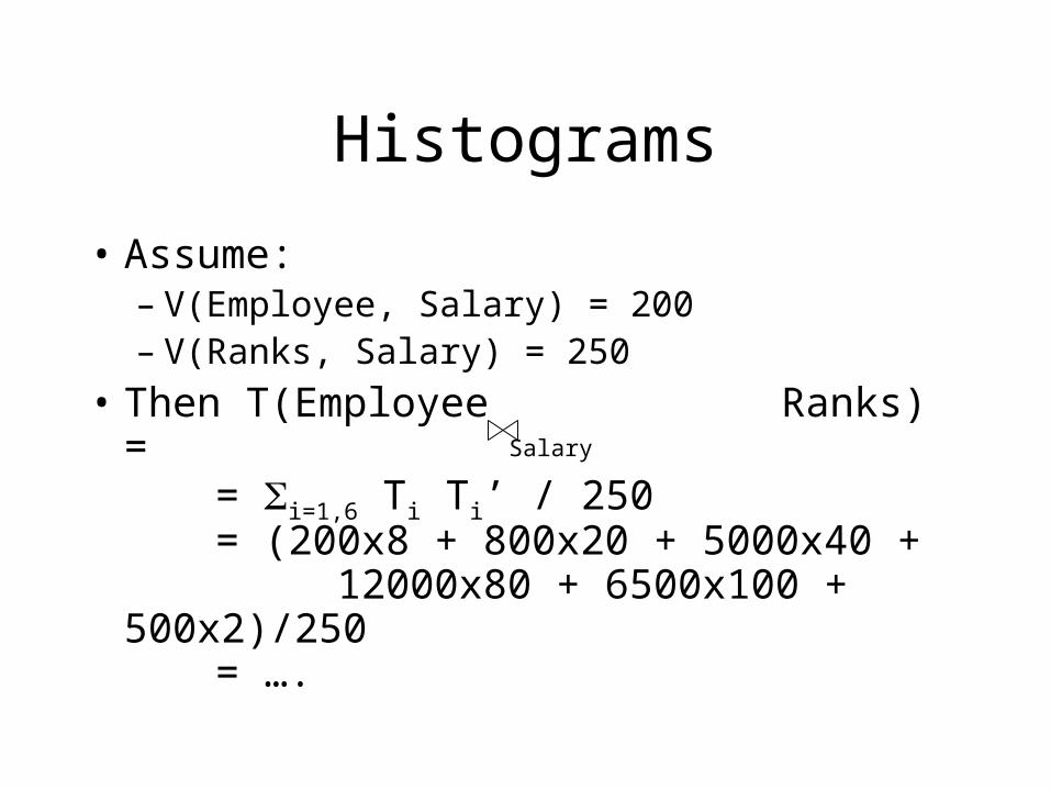
• Assume:– V(Employee, Salary) = 200– V(Ranks, Salary) = 250

• Then T(Employee Ranks) == i=1,6 Ti Ti’ / 250= (200x8 + 800x20 + 5000x40 + 12000x80 + 6500x100 +

500x2)/250= ….

Salary

Plans for Single-Relation Queries(Prep for Join ordering)

Plans for Single-Relation Queries(Prep for Join ordering)

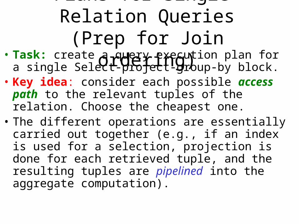
• Task: create a query execution plan for a single Select-project-group-by block.

• Key idea: consider each possible access path to the relevant tuples of the relation. Choose the cheapest one.

• The different operations are essentially carried out together (e.g., if an index is used for a selection, projection is done for each retrieved tuple, and the resulting tuples are pipelined into the aggregate computation).

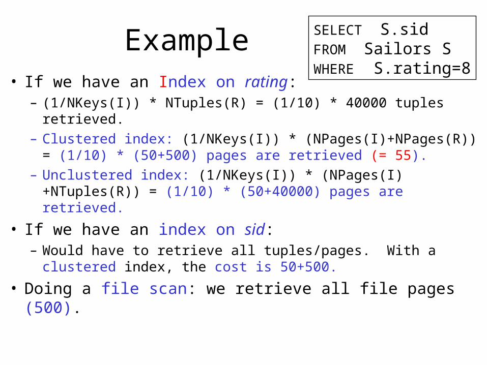
Example• If we have an Index on rating:

– (1/NKeys(I)) * NTuples(R) = (1/10) * 40000 tuples retrieved.

– Clustered index: (1/NKeys(I)) * (NPages(I)+NPages(R)) = (1/10) * (50+500) pages are retrieved (= 55).

– Unclustered index: (1/NKeys(I)) * (NPages(I)+NTuples(R)) = (1/10) * (50+40000) pages are retrieved.

• If we have an index on sid:– Would have to retrieve all tuples/pages. With a clustered index,

the cost is 50+500.

• Doing a file scan: we retrieve all file pages (500).

SELECT S.sidFROM Sailors SWHERE S.rating=8

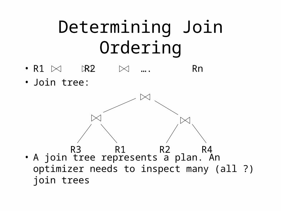
Determining Join Ordering

• R1 R2 …. Rn• Join tree:

• A join tree represents a plan. An optimizer needs to inspect many (all ?) join trees

R3 R1 R2 R4

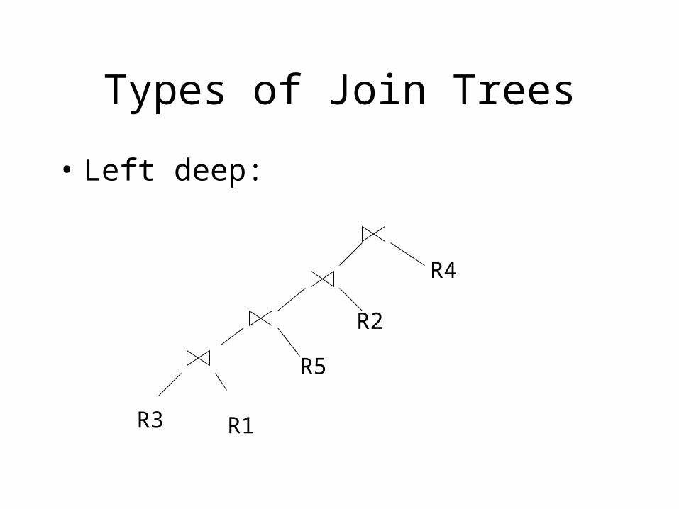
Types of Join Trees

• Left deep:

R3 R1

R5

R2

R4

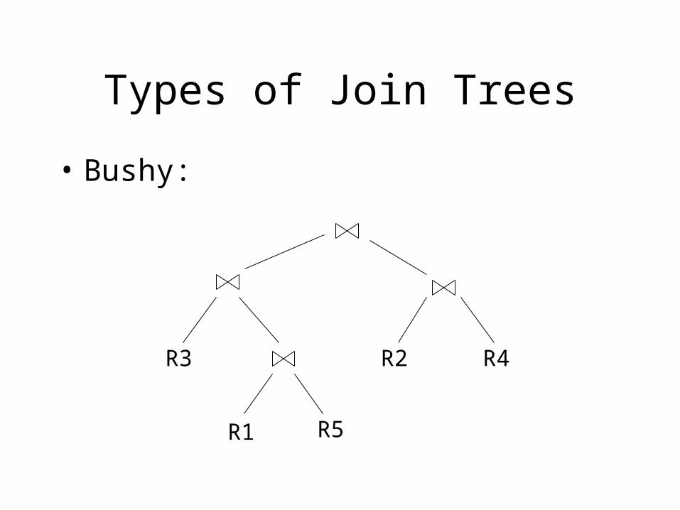
Types of Join Trees

• Bushy:

R3

R1

R2 R4

R5

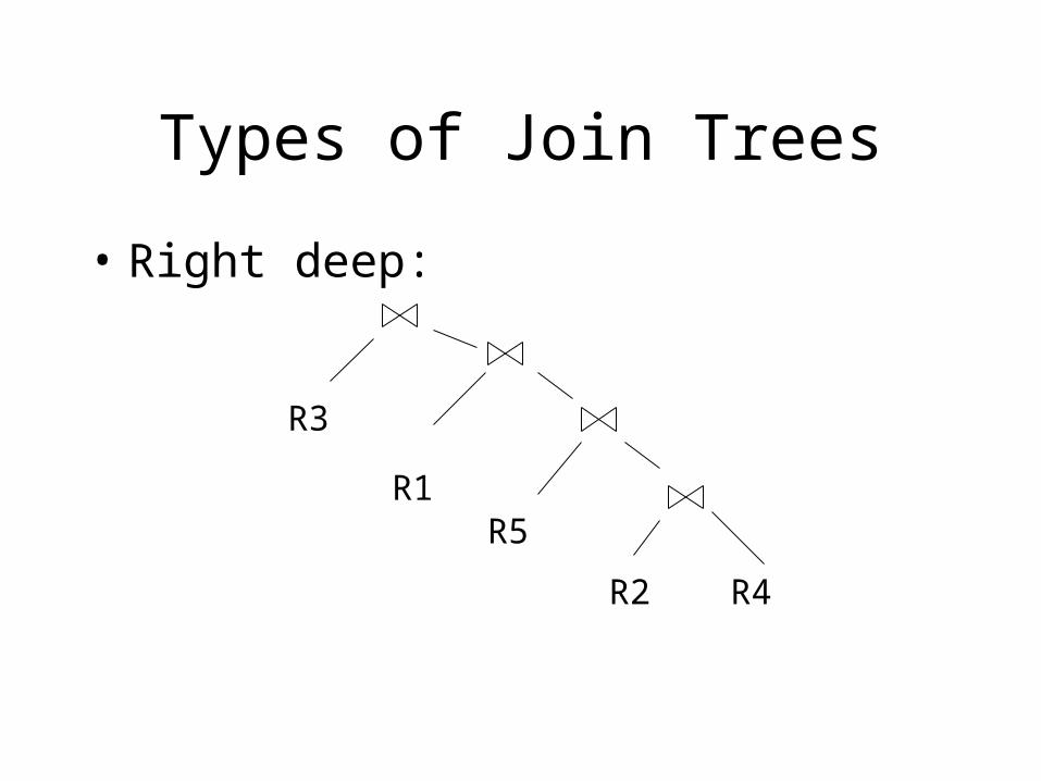
Types of Join Trees

• Right deep:

R3

R1R5

R2 R4

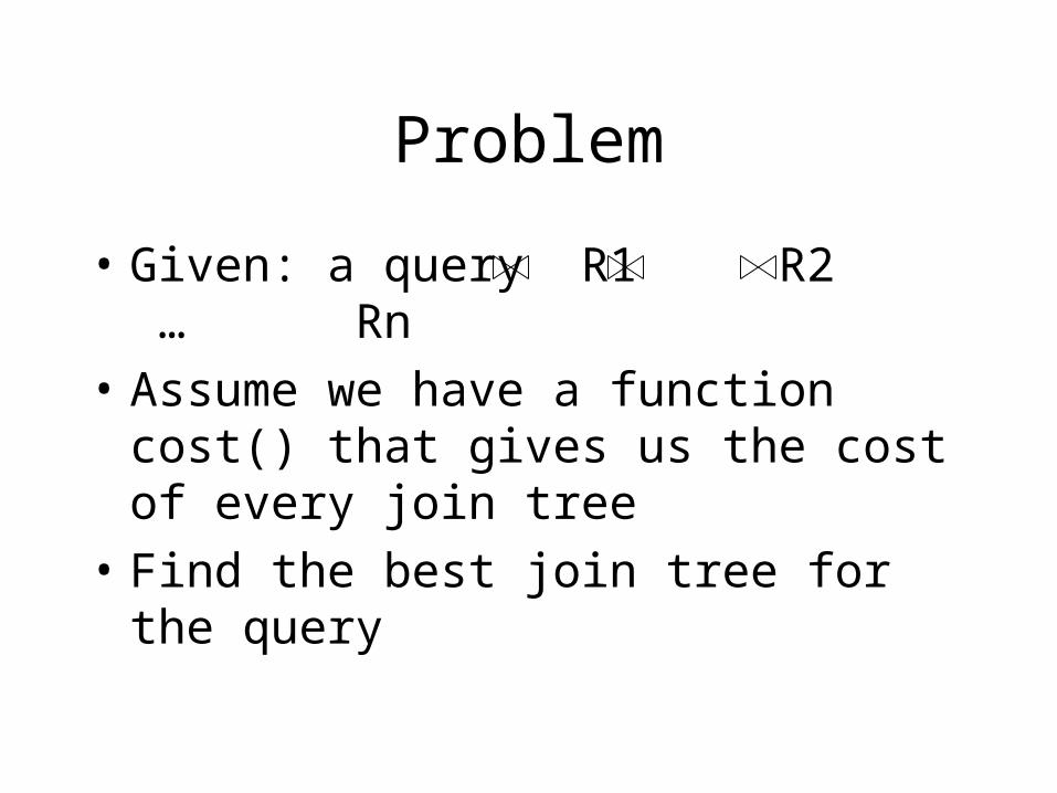
Problem

• Given: a query R1 R2 … Rn

• Assume we have a function cost() that gives us the cost of every join tree

• Find the best join tree for the query

Dynamic Programming

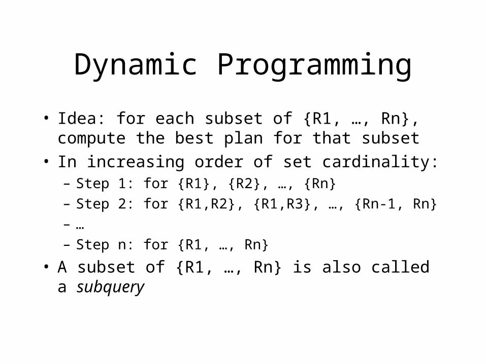
• Idea: for each subset of {R1, …, Rn}, compute the best plan for that subset

• In increasing order of set cardinality:– Step 1: for {R1}, {R2}, …, {Rn}

– Step 2: for {R1,R2}, {R1,R3}, …, {Rn-1, Rn}

– …

– Step n: for {R1, …, Rn}

• A subset of {R1, …, Rn} is also called a subquery

Dynamic Programming

• For each subquery Q ⊆ {R1, …, Rn} compute the following:– Size(Q)– A best plan for Q: Plan(Q)– The cost of that plan: Cost(Q)

Dynamic Programming

• Step 1: For each {Ri} do:– Size({Ri}) = B(Ri)– Plan({Ri}) = Ri– Cost({Ri}) = (cost of scanning Ri)

Dynamic Programming

• Step i: For each Q ⊆ {R1, …, Rn} of cardinality i do:– Compute Size(Q) (later…)– For every pair of subqueries Q’, Q’’

s.t. Q = Q’ U Q’’compute cost(Plan(Q’) Plan(Q’’))

– Cost(Q) = the smallest such cost– Plan(Q) = the corresponding plan

Dynamic Programming

• Return Plan({R1, …, Rn})

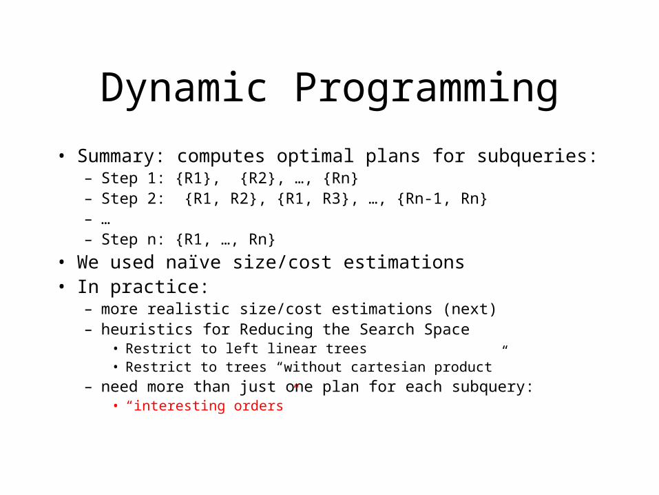
Dynamic Programming

• Summary: computes optimal plans for subqueries:– Step 1: {R1}, {R2}, …, {Rn}– Step 2: {R1, R2}, {R1, R3}, …, {Rn-1, Rn}– …– Step n: {R1, …, Rn}

• We used naïve size/cost estimations• In practice:

– more realistic size/cost estimations (next)– heuristics for Reducing the Search Space

• Restrict to left linear trees• Restrict to trees “without cartesian product”

– need more than just one plan for each subquery:• “interesting orders”