remote sensing

Article

Radiometric Correction and 3D Integration ofLong-Range Ground-Based Hyperspectral Imageryfor Mineral Exploration of Vertical Outcrops

Sandra Lorenz 1,*, Sara Salehi 2,3, Moritz Kirsch 1, Robert Zimmermann 1 ID , Gabriel Unger 1,Erik Vest Sørensen 2 ID and Richard Gloaguen 1 ID

1 Helmholtz-Zentrum Dresden-Rossendorf, Helmholtz Institute Freiberg for Resource Technology,Division “Exploration Technology”, Chemnitzer Straße 40, 09599 Freiberg, Germany;m.kirsch@hzdr.de (M.K.); r.zimmermann@hzdr.de (R.Z.); g.unger@hzdr.de (G.U.); r.gloaguen@hzdr.de (R.G.)

2 Department of Petrology and Economic Geology, Geological Survey of Denmark and Greenland,1350 Copenhagen K, Denmark; ssal@geus.dk (S.S.); evs@geus.dk (E.V.S.)

3 Department of Geosciences and Natural Resource Management, University of Copenhagen,1165 Copenhagen K, Denmark

* Correspondence: s.lorenz@hzdr.de; Tel.: +49-351-260-4487

Received: 22 December 2017; Accepted: 24 January 2018; Published: 26 January 2018

Abstract: Recently, ground-based hyperspectral imaging has come to the fore, supporting the arduoustask of mapping near-vertical, difficult-to-access geological outcrops. The application of outcropsensing within a range of one to several hundred metres, including geometric corrections andintegration with accurate terrestrial laser scanning models, is already developing rapidly. However,there are few studies dealing with ground-based imaging of distant targets (i.e., in the range ofseveral kilometres) such as mountain ridges, cliffs, and pit walls. In particular, the extreme influenceof atmospheric effects and topography-induced illumination differences have remained an unmetchallenge on the spectral data. These effects cannot be corrected by means of common correction toolsfor nadir satellite or airborne data. Thus, this article presents an adapted workflow to overcome thechallenges of long-range outcrop sensing, including straightforward atmospheric and topographiccorrections. Using two datasets with different characteristics, we demonstrate the application ofthe workflow and highlight the importance of the presented corrections for a reliable geologicalinterpretation. The achieved spectral mapping products are integrated with 3D photogrammetricdata to create large-scale now-called “hyperclouds”, i.e., geometrically correct representations of thehyperspectral datacube. The presented workflow opens up a new range of application possibilities ofhyperspectral imagery by significantly enlarging the scale of ground-based measurements.

Keywords: hyperspectral; topographic correction; atmospheric correction; radiometric correction;long-range; long-distance; Structure from Motion (SfM); photogrammetry; mineral mapping;minimum wavelength mapping; Maarmorilik; Riotinto

1. Introduction

Hyperspectral imaging has been increasingly used to support mineral exploration and geologicalmapping campaigns. The obtained spectral signatures provide detailed information about thecomposition of rocks and the occurrence of economic minerals. The hyperspectral instruments areconventionally operated with a nadir viewing angle, comprising different scales of area coverageand spatial resolution by operation on satellite [1,2], airplane [3–6] or drone [7]. Dependingon the acquisition altitude, a varying influence of the atmosphere between sensor and target,as well as illumination differences due to topography, can be observed in the acquired spectral

Remote Sens. 2018, 10, 176; doi:10.3390/rs10020176 www.mdpi.com/journal/remotesensing

Remote Sens. 2018, 10, 176 2 of 23

imagery. Numerous approaches have been introduced in an attempt to overcome these effects:Atmospheric influences are either corrected by atmospheric modelling using radiative transfer models(e.g., [8–10]), the use of ground targets with known or assumed spectra (empirical line calibration [11],flat field correction [12], dark object subtraction [13]), or a combination of both [14]. Whereas radiativetransfer models rely on the correct input of a set of external parameters and are mainly used forsatellite and airborne data, the use of ground targets, dark objects, or flat fields provides a much morestraightforward approach. However, these methods require a spatial resolution high enough to resolvespectrally uniform reference target(s) and/or a reasonable knowledge on the spectra of those materialspresent, and are therefore mainly used for drone- or airborne data with low acquisition altitudes(e.g., [7,15]).

In the last few years, a ground-based approach of using hyperspectral sensors for geologicalapplications has emerged. A tripod-mounted device can be used to rapidly acquire spectrally andspatially highly resolved data of near-vertical geological outcrops, i.e., spatial orientations that arenot (or hardly) observable by nadir-faced instruments. Near-vertical outcrops may comprise steepmountain slopes, water-faced cliffs, open pit mine walls, and road cuts. Particularly in arctic or humidregions, where snow and ice, lichens, or dense vegetation cover the Earth’s surface, the investigation ofsuch natural or artificial cuts through the strata might be the only possibility to obtain spectralinformation of the local geology. Currently, ground-based hyperspectral sensors for geologicalapplications are nearly exclusively used for targets at distances between one to several hundredmetres (e.g., [16–18]). Within this range, the spatial resolution varies between centimetre and decimetrescale, enough to resolve even small-scale mineral compounds and fault systems. Another significantbenefit of close-distance measurements is the negligible influence of the atmosphere, which potentiallyvoids the need for an elaborate radiometric correction. Instead, an empirical line approach usingreference targets with the same orientation, distance, and illumination conditions as the geologicaltarget is sufficient for the conversion to reflectance. However, observing a geological target at closerange is not always feasible or reasonable. In particular, larger and vertically oriented targets suchas steep mountain slopes, sea- or lake-faced cliffs, and walls of large open pit mines are often onlyfully visible from an opposing location such as a neighbouring mountain [19], pit level, shore, or evena boat [20]. The distance between the sensor and the target of interest can then easily exceed theclose-range and extend to several kilometres. These distances not only lead to major atmosphericdistortions, but also prevent the logistical setup of visible reference targets for radiometric correction aswell as ground control points for image georeferencing. Additionally, owing to the much larger scale ofthe observed surface and the ground-based viewing perspective, pixels within one scene can representa range of different distances and orientations, leading to highly variable radiometric distortions.For those reasons, correction methods established for nadir acquisitions are not applicable or need tobe intensely modified to account for the special conditions of long-range ground-based sensing.

In this paper, we meet these additional challenges and present a novel workflow that allowsthe creation of fully corrected long-range ground-based hyperspectral image data for geologicalapplications. In addition to sensor-induced geometric distortion corrections, the workflow nowincludes a new approach for the radiometric correction of long-range ground-based data as well as atopographic correction algorithm based on integration with 3D surface data using automatic matchingalgorithms. We also describe a detailed methodology for producing 3D hyperclouds, i.e., geometricallycorrect representations of the hyperspectral datacube, for the display of generated spectral mappingproducts. The methods presented will be included in the open source Mineral Exploration PythonHyperspectral Toolbox MEPHySTo [7]. We demonstrate the methodology in two areas that differ ingeology, climate, and scientific objectives. The first area is located in an arctic environment, where twohyperspectral scans acquired from different points of view are used to detect and map mineralogicalvariations in the composition of the Mârmorilik Formation marbles in West Greenland. The singleresult map is integrated with photogrammetry data to provide spatial context and a 3D view that canbe integrated into 3D modelling. The second dataset was acquired at the now-abandoned open pit

Remote Sens. 2018, 10, 176 3 of 23

mine Corta Atalaya near Minas de Riotinto, Spain. The Spanish dataset demonstrates the applicabilityof the corrected dataset for alteration zone mapping of a massive sulphide deposit under hot anddusty conditions as well as the integratability of datasets acquired at different times.

2. Areas of Investigation

2.1. Nunngarut Peninsula, Maarmorilik, Greenland

The first study area is located in central West Greenland, within the regions of Uummannaq Fjordand Karrat Isfjord (Figure 1). The investigated area covers large parts of the Nunngarut Peninsulaat the Qaamarujuk fjord, where the former mining town of Maarmorilik is located. The nearbyBlack Angle Pb–Zn deposit is separated from the Nunngarut Peninsula by the smaller Affarlikassaafjord. The study area belongs to the Mârmorilik Formation, a 1600 m thick carbonate-dominated rocksequence representing the southernmost stratigraphy of the Paleoproterozoic Karrat Group [21]. It wasdeposited between 2.1 and 1.9 Ga in an epicontinental marginal basin as platform carbonates [21],nonconformably overlies a suite of strong deformed Archean orthogneisses, and is overlain byflysch-type metasedimentary rocks of the Nûkavsak Formation [22].

The Mârmorilik Formation is dominated by dolomite-rich marbles in the lower part and calcite-richmarbles in the upper part. Locally, interbedded horizons of quartzites, tremolite-rich marblesand possible metamorphosed evaporites in the form of anhydrite occur [21,23]. The Black AngelMississippi-Valley-Type (MVT) Pb–Zn deposit is emplaced within the Mârmorilik Formation [22,24],causing an overprint of the marbles by basal brines. The whole succession of Archean basement and theKarrat Group was strongly folded and thrusted by the Nagssugtoqidian–Rinkian orogenesis. During thisorogenesis, the Mârmorilik Formation underwent at least three phases of deformation [19], leading torecrystallisation and metamorphism under high greenschist to amphibolite facies conditions [25].The Mârmorilik Formation is interpreted to be the lateral equivalent to the Qaarsukassak Formation [26],and together they form a several hundred square kilometre large prospective region for zincmineralisation [19,27].

2.2. Corta Atalaya, Riotinto, Spain

Corta Atalaya, near Minas de Riotinto in the province of Huelva (southern Spain), is, with a sizeof 1200 × 900 m and a maximal depth of 365 m, one of the most famous open pits of the Riotintomining district (Figure 1). The Volcanogenic Massive Sulphide (VMS) mineralisation of Riotinto isassociated with the Iberian Pyrite Belt (IPB), which is considered to host the largest concentrationof massive sulphides in the Earth’s crust [28]. The IPB is located in a north-vergent fold and thrustbelt of late Variscan age [29] extending from east of Setubal, Portugal, to north of Seville, Spain, andhas been extensively mined for copper, manganese, iron, and gold since the Bronze Age. At Riotinto,the lithostratigraphic succession can be divided into three units (from bottom to top): (i) phyllitesand quartzites; (ii) slates, basalt sills, felsic volcanics (rhyolites and dacites); and (iii) the so-calledCulm series (greywackes and slates). The stratabound, VMS lenses are located within felsic volcanicsof Upper Devonian to Lower Carboniferous ages [28]. Zones of chloritic and argillitic alteration areassociated with the massive sulphide mineralisation. Stockwork zones occur underneath the lenses inthe vicinity of faults [28]. A gossan usually forms in the cap-rock above. The deposit of Riotinto itselfis situated in the hinge of an E–W-trending anticline with an east-plunging fold axis. Corta Atalaya islocated on the southern flank of this so-called Riotinto anticline. Stockwork and massive ore bodiesare associated with E–W-striking thrusts. A set of later NW–SE-oriented transverse faults offsetsthe Riotinto anticline. The most prominent of these faults, the Falla Eduardo, displaces the massivesulphide body San Dionisio about 150 m to the south and finds its continuation in the Filón Sur orebody east of Corta Atalaya [28]. The massive sulphide body San Dionisio, which was exploited inCorta Atalaya, originally had reserves of 100 million tonnes. Originally, the mine was dedicated tothe extraction of iron and copper sulphides (mainly pyrite with smaller amounts of chalcopyrite).

Remote Sens. 2018, 10, 176 4 of 23

The initial objective was to extract copper from copper sulphides, but, subsequently, the sulphurcontained in pyrite was used for the manufacturing of sulphuric acid until final closure of the open pitin 1991 [28].

Remote Sens. 2018, 10, x FOR PEER REVIEW 4 of 23

chalcopyrite). The initial objective was to extract copper from copper sulphides, but, subsequently, the sulphur contained in pyrite was used for the manufacturing of sulphuric acid until final closure of the open pit in 1991 [28].

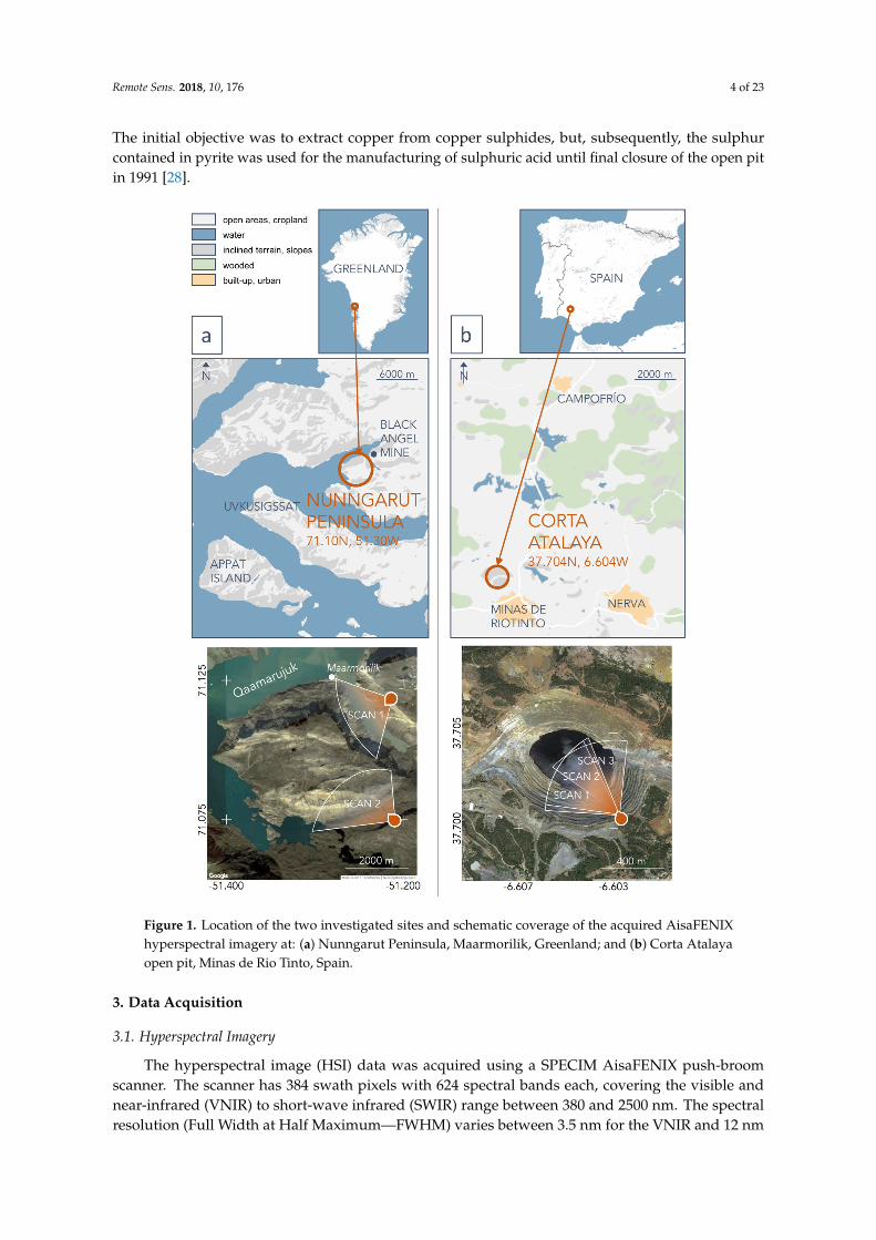
Figure 1. Location of the two investigated sites and schematic coverage of the acquired AisaFENIX hyperspectral imagery at: (a) Nunngarut Peninsula, Maarmorilik, Greenland; and (b) Corta Atalaya open pit, Minas de Rio Tinto, Spain.

3. Data Acquisition

3.1. Hyperspectral Imagery

The hyperspectral image (HSI) data was acquired using a SPECIM AisaFENIX push-broom scanner. The scanner has 384 swath pixels with 624 spectral bands each, covering the visible and near-

Figure 1. Location of the two investigated sites and schematic coverage of the acquired AisaFENIXhyperspectral imagery at: (a) Nunngarut Peninsula, Maarmorilik, Greenland; and (b) Corta Atalayaopen pit, Minas de Rio Tinto, Spain.

3. Data Acquisition

3.1. Hyperspectral Imagery

The hyperspectral image (HSI) data was acquired using a SPECIM AisaFENIX push-broomscanner. The scanner has 384 swath pixels with 624 spectral bands each, covering the visible andnear-infrared (VNIR) to short-wave infrared (SWIR) range between 380 and 2500 nm. The spectralresolution (Full Width at Half Maximum—FWHM) varies between 3.5 nm for the VNIR and 12 nm

Remote Sens. 2018, 10, 176 5 of 23

in the SWIR at a spectral sampling distance of about 1.5 nm (VNIR) and 5 nm (SWIR), respectively.By mounting the instrument on a rotary stage, a continuous hyperspectral image with a vertical fieldof view (FOV) of 32.3◦ and a maximum scanning angle of 130◦ could be acquired in one measurement.During the measurements, the GPS position of the camera, acquisition time, and general viewingdirection (from here on referred to as ‘camera angle’) of the scan were recorded. A Spectralon SRS-99white panel was set up near the camera within the FOV and with a similar general orientation as theimaged outcrop.

3.2. Photogrammetry Data/3D Data

Images for reconstruction of surface geometry were recorded using precalibrated RGB andhyperspectral cameras. In the case of Maarmorilik, a Nikon D800E with a 35 mm 1.4 Zeiss lens wasused from a helicopter. The 3D pointcloud of Corta Atalaya was based on fusion of drone-borneimages from a Rikola Hyperspectral Imager (red band) and a Canon EOS M with EF-M 22 mm f/2 STMlens (as grey-scale image). Camera positions were obtained from an attached GPS device, whereasthe imaging geometry was reconstructed using a Structure from Motion (SfM) and MultiView Stereo(MVS) workflow. Prior to the photogrammetry workflow, image distortions were removed.

3.3. Validation Sampling

Samples of the main lithologies were taken for a validation of the correction workflow and of themineral mapping results. Sample locations were recorded using a handheld GPS device. Spectra ofrepresentative fresh and altered rock surfaces were acquired in situ using a portable Spectral EvolutionPSR-3500 spectro-radiometer using a contact probe (8 mm spot size) with an internal, artificial lightsource. Its spectral resolution is 3.5 nm (1.5 nm sampling interval) in VNIR and 7 nm (2.5 nmsampling interval) in the SWIR, resulting in 1024 channels in the spectral range from 350 to 2500 nm.Radiance values were converted to reflectance using a calibrated PTFE panel with >99% reflectance inVNIR and >95% in SWIR (either Spectralon SRS-99 or Zenith Polymer). Each spectral record consistedof 10 individual measurements, which were taken consecutively and then averaged.

4. Processing Workflow

4.1. Preprocessing of Hyperspectral Raw Data

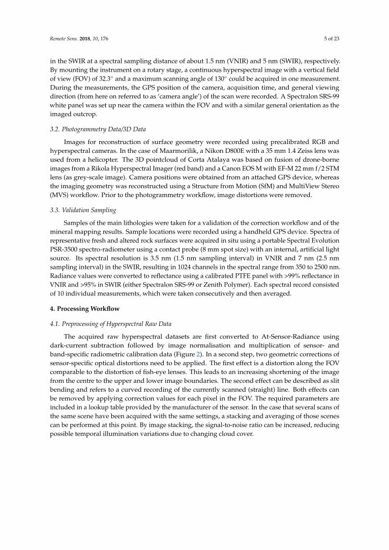
The acquired raw hyperspectral datasets are first converted to At-Sensor-Radiance usingdark-current subtraction followed by image normalisation and multiplication of sensor- andband-specific radiometric calibration data (Figure 2). In a second step, two geometric corrections ofsensor-specific optical distortions need to be applied. The first effect is a distortion along the FOVcomparable to the distortion of fish-eye lenses. This leads to an increasing shortening of the imagefrom the centre to the upper and lower image boundaries. The second effect can be described as slitbending and refers to a curved recording of the currently scanned (straight) line. Both effects canbe removed by applying correction values for each pixel in the FOV. The required parameters areincluded in a lookup table provided by the manufacturer of the sensor. In the case that several scans ofthe same scene have been acquired with the same settings, a stacking and averaging of those scenescan be performed at this point. By image stacking, the signal-to-noise ratio can be increased, reducingpossible temporal illumination variations due to changing cloud cover.

Remote Sens. 2018, 10, 176 6 of 23Remote Sens. 2018, 10, x FOR PEER REVIEW 6 of 23

Figure 2. Schematic workflow for the correction, processing, and 3D integration of long-range ground-based hyperspectral imagery.

4.2. Radiometric Correction of Hyperspectral Radiance Data

Subsequent to the transformation of the raw hyperspectral data into radiance, a conversion to at-sensor reflectance needs to be applied, which can be achieved using a white reference panel placed near the sensor. This Spectralon (SRS-99) reference target is close to an ideal Lambertian reflector with >99% reflectance in the VNIR and >95% in the SWIR. Its exact reflectance spectrum is known and can be used for an empirical line correction of the radiance data. Hereby, a linear regression between the image radiance values and the reference reflectance values is calculated and applied for each band.

Depending on the imaging distance and the climatic conditions, the resulting at-sensor reflectance image may still feature atmospheric distortions (see Figure 3). In contrast to air- or spaceborne data, the scene-specific intermediate atmospheric layer can be assumed to have a uniform composition with only negligible variations. Nevertheless, the amount of atmospheric influence varies for each pixel and depends mainly on the distance between sensor and target, but can be also influenced by local variations, e.g., differing intensities of upwelling water vapour.

Figure 2. Schematic workflow for the correction, processing, and 3D integration of long-rangeground-based hyperspectral imagery.

4.2. Radiometric Correction of Hyperspectral Radiance Data

Subsequent to the transformation of the raw hyperspectral data into radiance, a conversion toat-sensor reflectance needs to be applied, which can be achieved using a white reference panel placednear the sensor. This Spectralon (SRS-99) reference target is close to an ideal Lambertian reflector with>99% reflectance in the VNIR and >95% in the SWIR. Its exact reflectance spectrum is known and canbe used for an empirical line correction of the radiance data. Hereby, a linear regression between theimage radiance values and the reference reflectance values is calculated and applied for each band.

Depending on the imaging distance and the climatic conditions, the resulting at-sensor reflectanceimage may still feature atmospheric distortions (see Figure 3). In contrast to air- or spaceborne data,the scene-specific intermediate atmospheric layer can be assumed to have a uniform composition withonly negligible variations. Nevertheless, the amount of atmospheric influence varies for each pixeland depends mainly on the distance between sensor and target, but can be also influenced by localvariations, e.g., differing intensities of upwelling water vapour.

Remote Sens. 2018, 10, 176 7 of 23Remote Sens. 2018, 10, x FOR PEER REVIEW 7 of 23

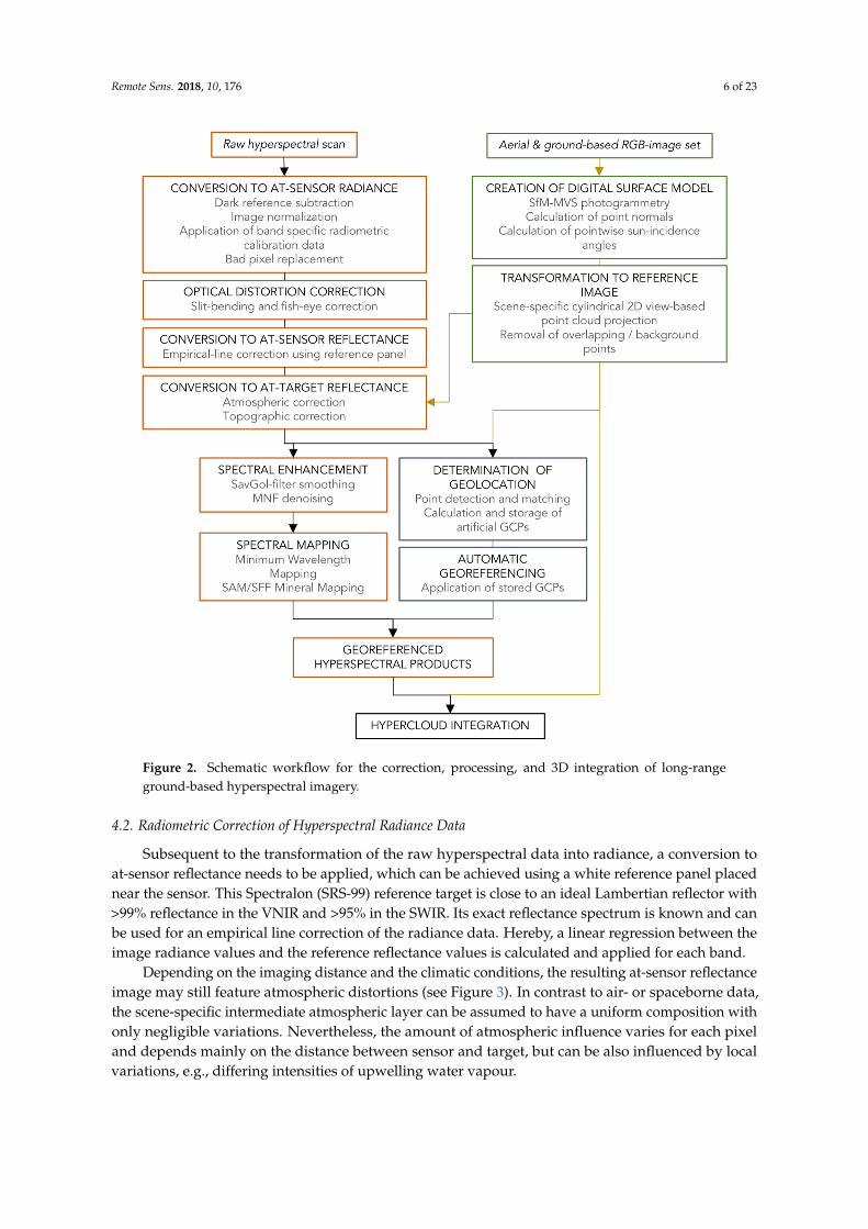
Figure 3. Atmospheric correction workflow on the example of the Maarmorilik marble cliffs (Nunngarut, Scan 2). Hyperspectral images are displayed using spectral true colour representative bands (R: 640 nm G: 550 nm B: 470 nm). See text for a detailed description. (a) Control spectra set; (b) continuum removal; (c) adjusted control spectra set; (d) final control spectrum and selection of the control feature.

Given these circumstances, we attempt to perform a radiometric correction to remove atmospheric distortions using a single atmospheric correction spectrum for each scene. The intensity of correction needs to be varied according to the amount of atmospheric distortion. For the correction approach to be robust and independent from additional parameters or knowledge about the composition of the influencing atmospheric layer, the atmospheric correction spectrum is derived

Figure 3. Atmospheric correction workflow on the example of the Maarmorilik marble cliffs(Nunngarut, Scan 2). Hyperspectral images are displayed using spectral true colour representativebands (R: 640 nm G: 550 nm B: 470 nm). See text for a detailed description. (a) Control spectra set;(b) continuum removal; (c) adjusted control spectra set; (d) final control spectrum and selection of thecontrol feature.

Given these circumstances, we attempt to perform a radiometric correction to remove atmosphericdistortions using a single atmospheric correction spectrum for each scene. The intensity of correctionneeds to be varied according to the amount of atmospheric distortion. For the correction approach

Remote Sens. 2018, 10, 176 8 of 23

to be robust and independent from additional parameters or knowledge about the compositionof the influencing atmospheric layer, the atmospheric correction spectrum is derived directlyand automatically from the hyperspectral image itself. Hereby, the correction spectrum is acomprehensive representation of all scene-abundant spectrally influencing atmospheric components,which may encompass atmospheric dust, water vapour, and other atmospheric gases. The correctionspectrum is neither selective nor restricted to defined components and is thus applicable for anyatmospheric setting.

Owing to the assumed constant composition of the atmosphere over the scene, the depthsof all atmosphere-related features should change equally if the atmospheric influence is altered.This approach allows us to evaluate the amount of atmospheric influence for each pixel by the depth ofonly one atmospheric absorption feature and eliminates the need for atmospheric models, additionalcalibration targets, and distance measurements. The now-called control feature must necessarily beboth common in all possibly occurring atmospheric compositions and strong enough to be detectableeven for low atmospheric influence. Additionally, it should not overlap with any characteristicmineralogy-related features to avoid interference and miscorrections. The absorption band we foundto fulfill these conditions best is situated at 1126 nm (Figure 3d) and is related to atmospheric watervapour [14].

The atmospheric correction workflow consists of several steps, which can also be retraced inFigure 3:

1. Masking of sky-related pixels: All image pixels representing sky and sky reflected by mirroringsurfaces such as water are masked out automatically from the reflectance image using a ratiobetween the image bands located at 410 and 890 nm. These wavelength positions are set toencompass two ends of the extreme decline in VNIR reflectance that is specific for sky-relatedspectra. This characteristic shape leads to a usually very distinct ratio difference between skyand non-sky pixels. In our examples, the masking threshold was most successful in a ratio rangebetween 1.0 and 2.0.

2. Determination and processing of possible correction spectra: The depth of the control featureat 1126 nm is calculated for all remaining pixels. All pixel spectra with a control feature depthwithin 80–100% of the maximum are extracted as a control spectrum set (Figure 3a), which willbe used to determine the final atmospheric correction spectrum. A continuum removal and anequalisation of the control feature depth are applied on each spectrum of the control set separately.The respective continuum hull is calculated using a linear interpolation of stepwise acquiredmaxima all over the respective spectrum (Figure 3b). The moving window for the continuumhull calculation can either be set to a fixed step size or restricted to specific stored wavelengthranges that are located outside or at the edge of known atmospheric absorption windows.

3. Exclusion of nonatmospheric features: Some spectra of the resulting equalised control spectra setmay still contain additional nonatmospheric absorptions. These features should be excluded fromthe correction spectrum to avoid a weakening or deletion of important mineralogical featuresduring the atmospheric correction process. In contrast to atmospheric features, nonatmosphericabsorptions occur with differing intensities and only in a spectral subset of the control spectra(Figure 3c,d). They can be excluded from the control spectrum set by maintaining only the highestof all spectral values for each wavelength. The used threshold can be varied manually if needed.

4. Calculation and application of the final control spectrum: The remaining spectral informationis averaged for each wavelength to reduce possible noise. The outcome of the whole procedureprovides a single continuum-removed correction spectrum containing solely the characteristicatmospheric contribution of the analysed hyperspectral image (Figure 3d). The atmosphericcorrection itself is performed pixelwise. For each pixel, the intensity of the correction spectrumneeds to be adjusted to both depth and reflectance value of the control feature in the pixelspectrum. The correction itself is then achieved by a simple division of the pixel spectrum by the

Remote Sens. 2018, 10, 176 9 of 23

adjusted correction spectrum. The original reflectance intensities are maintained in the correctedimage spectra during that process.

The processing time for the automatic correction of a hyperspectral scan with the spatial andspectral dimensions as in our examples is less than one minute. Thus, the method is extremely time-and effort-saving and can be easily integrated into a batch-processing workflow.

Depending on the Signal-to-Noise ratio (SNR) of the processed dataset, a subsequent MinimumNoise Fraction (MNF) smoothing can be advantageous. MNF smoothing entails a transformation of theimage into MNF space, a rejection of bands with low SNR, and a subsequent back-transformation intothe original image space [30]. The number of MNF bands to be rejected can be determined by lookingat the eigenvalue function of the calculated MNF bands, which reaches a plateau after a sharp increaseand suggests a rejection if the asymptotic eigenvalue function approaches a linear function [31].

4.3. SfM-MVS Photogrammetry

The Digital Surface Model is derived from aerial and ground-based images using theStructure-from-Motion MultiView Stereo (SfM-MVS) algorithms in Agisoft Photoscan Professional 1.2.5.SfM-MVS is a low-cost, user-friendly workflow combining photogrammetric techniques, 3D computervision, and conventional surveying techniques. It solves the equations for camera pose and scenegeometry automatically using a highly redundant bundle adjustment [32,33]. A typical SfM-MVSworkflow towards a final surface model consists of the following eight steps [33,34]:

1. Detection of characteristic image points;2. Automatic point matching using a homologous transformation;3. Keypoint filtering—this step is crucial for model accuracy and validation of later results [35];4. Iterative bundle adjustment to reconstruct the image acquisition geometry and internal

camera parameters;5. Scaling and georeferencing of the intrinsic coordinate system to available reference points (GCPs)

or camera coordinates and optimisation of the resulting sparse cloud;6. Applying MultiView Stereo algorithms (dense matching) to compute the dense cloud—the

resulting dense cloud is the basis for the geometric correction of the hyperspectral data;7. Interpolation of the dense cloud by, e.g., Meshing or Inverse Distance Weighting (IDW), to retrieve

a Digital Surface Model (DSM);8. Texturising of the 3D model.

4.4. Calculation of Sun Incidence Angles for Topographic Correction

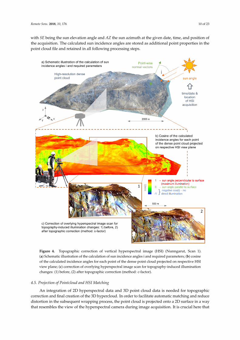
Knowledge of the sun incidence angle for each pixel of the hyperspectral image is crucial for itstopographic correction. In contrast to nadir data, vertical outcrop scans can have multiple pixels locatedat any given latitude/longitude coordinate position, which can be only spatially differentiated by theirelevation values. Therefore, common tools for the calculation of slope, aspect, and sun incidence angleof Digital Elevation Models (DEM) cannot be applied here. Instead, we calculate the sun incidenceangle for each individual point of the point cloud generated in Section 4.3 as the angle between thepoint normal and the sun vector (Figure 4a). The point normals were either calculated during thepoint cloud construction or can be computed retroactively using a triangulation of neighboring points.The sun vector is characterised by

sunvec =

cos(SE) ∗ sin(AZ)cos(SE) ∗ cos(AZ)

sin(AZ)

(1)

Remote Sens. 2018, 10, 176 10 of 23

with SE being the sun elevation angle and AZ the sun azimuth at the given date, time, and position ofthe acquisition. The calculated sun incidence angles are stored as additional point properties in thepoint cloud file and retained in all following processing steps.Remote Sens. 2018, 10, x FOR PEER REVIEW 10 of 23

Figure 4. Topographic correction of vertical hyperspectral image (HSI) (Nunngarut, Scan 1). (a) Schematic illustration of the calculation of sun incidence angles i and required parameters; (b) cosine of the calculated incidence angles for each point of the dense point cloud projected on respective HSI view plane; (c) correction of overlying hyperspectral image scan for topography-induced illumination changes: (1) before, (2) after topographic correction (method: c-factor).

4.5. Projection of Pointcloud and HSI Matching

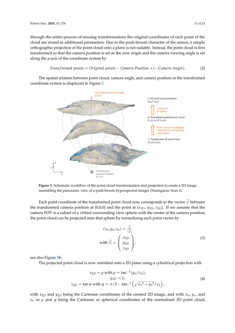
An integration of 2D hyperspectral data and 3D point cloud data is needed for topographic correction and final creation of the 3D hypercloud. In order to facilitate automatic matching and reduce distortion in the subsequent wrapping process, the point cloud is projected onto a 2D surface in a way that resembles the view of the hyperspectral camera during image acquisition. It is crucial here that through the entire process of ensuing transformations the original coordinates of each point of the cloud are stored as additional parameters. Due to the push-broom character of the sensor, a simple orthographic projection of the point cloud onto a plane is not suitable. Instead, the point cloud is first transformed so that the camera position is set as the new origin and the camera viewing angle is set along the y-axis of the coordinate system by

Figure 4. Topographic correction of vertical hyperspectral image (HSI) (Nunngarut, Scan 1).(a) Schematic illustration of the calculation of sun incidence angles i and required parameters; (b) cosineof the calculated incidence angles for each point of the dense point cloud projected on respective HSIview plane; (c) correction of overlying hyperspectral image scan for topography-induced illuminationchanges: (1) before, (2) after topographic correction (method: c-factor).

4.5. Projection of Pointcloud and HSI Matching

An integration of 2D hyperspectral data and 3D point cloud data is needed for topographiccorrection and final creation of the 3D hypercloud. In order to facilitate automatic matching and reducedistortion in the subsequent wrapping process, the point cloud is projected onto a 2D surface in a waythat resembles the view of the hyperspectral camera during image acquisition. It is crucial here that

Remote Sens. 2018, 10, 176 11 of 23

through the entire process of ensuing transformations the original coordinates of each point of thecloud are stored as additional parameters. Due to the push-broom character of the sensor, a simpleorthographic projection of the point cloud onto a plane is not suitable. Instead, the point cloud is firsttransformed so that the camera position is set as the new origin and the camera viewing angle is setalong the y-axis of the coordinate system by

Trans f ormed points = Original points− Camera Position ∗ (−Camera Angle). (2)

The spatial relation between point cloud, camera angle, and camera position in the transformedcoordinate system is displayed in Figure 5.

Remote Sens. 2018, 10, x FOR PEER REVIEW 11 of 23

= ∗ ( ). (2)

The spatial relation between point cloud, camera angle, and camera position in the transformed coordinate system is displayed in Figure 5.

Figure 5. Schematic workflow of the point cloud transformation and projection to create a 2D image resembling the panoramic view of a push-broom hyperspectral imager (Nunngarut, Scan 2).

Each point coordinate of the transformed point cloud now corresponds to the vector between the transformed camera position at (0,0,0) and the point at ( , , ). If we assume that the camera FOV is a subset of a virtual surrounding view sphere with the center at the camera position, the point cloud can be projected onto that sphere by normalizing each point vector by ( , , ) = | |

with = ; (3)

see also Figure 5b. The projected point cloud is now unfolded onto a 2D plane using a cylindrical projection with = with = tan ( ⁄ ) , = 1, = tan with = 2⁄ tan + , (4)

with and being the Cartesian coordinates of the created 2D image, and with , , and or and being the Cartesian or spherical coordinates of the normalised 3D point cloud, respectively (Figure 5c). The angle at which the cylinder is cut for the projection can be set by an additional parameter.

The projection into 2D space considers all of the points in the true line of sight of the hyperspectral camera, which includes points hidden behind points in the foreground (front points), such as the backside of a mountain (back points). This leads to artefacts within the created 2D image (see Figure 6a) and would adversely affect subsequent processing steps. Using a maximum threshold for the original spatial distance between neighbouring points, the adverse back points can be removed. To ensure a fast processing even for huge point clouds, a moving window is used to process several points at once. For each applied window, the contained point with the closest distance to the

Figure 5. Schematic workflow of the point cloud transformation and projection to create a 2D imageresembling the panoramic view of a push-broom hyperspectral imager (Nunngarut, Scan 2).

Each point coordinate of the transformed point cloud now corresponds to the vector→v between

the transformed camera position at (0,0,0) and the point at (x3D, y3D, z3D). If we assume that thecamera FOV is a subset of a virtual surrounding view sphere with the center at the camera position,the point cloud can be projected onto that sphere by normalizing each point vector by

(xn, yn, zn) =→v|→v |

with→v =

x3Dy3Dz3D

;(3)

see also Figure 5b.The projected point cloud is now unfolded onto a 2D plane using a cylindrical projection with

x2D = ρ with ρ = tan−1(yn/xn),y2D = 1,

z2D = tan ϕ with ϕ = π/2− tan−1(√

xn2 + yn2/zn

),

(4)

with x2D and y2D being the Cartesian coordinates of the created 2D image, and with xn, yn, andzn or ρ and ϕ being the Cartesian or spherical coordinates of the normalised 3D point cloud,

Remote Sens. 2018, 10, 176 12 of 23

respectively (Figure 5c). The angle at which the cylinder is cut for the projection can be set byan additional parameter.

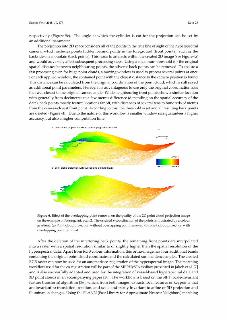
The projection into 2D space considers all of the points in the true line of sight of the hyperspectralcamera, which includes points hidden behind points in the foreground (front points), such as thebackside of a mountain (back points). This leads to artefacts within the created 2D image (see Figure 6a)and would adversely affect subsequent processing steps. Using a maximum threshold for the originalspatial distance between neighbouring points, the adverse back points can be removed. To ensure afast processing even for huge point clouds, a moving window is used to process several points at once.For each applied window, the contained point with the closest distance to the camera position is found.This distance can be calculated from the original coordination of the point cloud, which is still savedas additional point parameters. Hereby, it is advantageous to use only the original coordination axisthat was closest to the original camera angle. While neighbouring front points show a similar locationwith generally from decimetres to a few metres difference (depending on the spatial accuracy of thedata), back points mostly feature locations far off, with distances of several tens to hundreds of metresfrom the camera-closest front point. According to this, the threshold is set and all resulting back pointsare deleted (Figure 6b). Due to the nature of this workflow, a smaller window size guarantees a higheraccuracy, but also a higher computation time.

Remote Sens. 2018, 10, x FOR PEER REVIEW 12 of 23

camera position is found. This distance can be calculated from the original coordination of the point cloud, which is still saved as additional point parameters. Hereby, it is advantageous to use only the original coordination axis that was closest to the original camera angle. While neighbouring front points show a similar location with generally from decimetres to a few metres difference (depending on the spatial accuracy of the data), back points mostly feature locations far off, with distances of several tens to hundreds of metres from the camera-closest front point. According to this, the threshold is set and all resulting back points are deleted (Figure 6b). Due to the nature of this workflow, a smaller window size guarantees a higher accuracy, but also a higher computation time.

Figure 6. Effect of the overlapping point removal on the quality of the 2D point cloud projection image on the example of Nunngarut, Scan 2. The original x-coordination of the points is illustrated by a colour gradient. (a) Point cloud projection without overlapping point removal; (b) point cloud projection with overlapping point removal.

After the deletion of the interfering back points, the remaining front points are interpolated into a raster with a spatial resolution similar to or slightly higher than the spatial resolution of the hyperspectral data. Apart from RGB colour information, this ortho-image has four additional bands containing the original point cloud coordinates and the calculated sun incidence angles. The created RGB raster can now be used for an automatic co-registration of the hyperspectral image. The matching workflow used for the co-registration will be part of the MEPHySTo toolbox presented in Jakob et al. [7] and is also successfully adapted and used for the integration of vessel-based hyperspectral data and 3D point clouds in an accompanying paper [20]. The workflow is based on the SIFT (Scale-invariant feature transform) algorithm [36], which, from both images, extracts local features or keypoints that are invariant to translation, rotation, and scale and partly invariant to affine or 3D projection and illumination changes. Using the FLANN (Fast Library for Approximate Nearest Neighbors) matching algorithm library [37], correlating point pairs between both keypoint sets are found. The best-matching point pairs are used as control points for a polynomial warping of the hyperspectral image to fit on the RGB raster. After the co-registration, each overlapping point of both datasets features high-resolution spectral data, geographic position, and elevation, as well as the sun incidence angle at the time of the acquisition.

Figure 6. Effect of the overlapping point removal on the quality of the 2D point cloud projection imageon the example of Nunngarut, Scan 2. The original x-coordination of the points is illustrated by a colourgradient. (a) Point cloud projection without overlapping point removal; (b) point cloud projection withoverlapping point removal.

After the deletion of the interfering back points, the remaining front points are interpolatedinto a raster with a spatial resolution similar to or slightly higher than the spatial resolution of thehyperspectral data. Apart from RGB colour information, this ortho-image has four additional bandscontaining the original point cloud coordinates and the calculated sun incidence angles. The createdRGB raster can now be used for an automatic co-registration of the hyperspectral image. The matchingworkflow used for the co-registration will be part of the MEPHySTo toolbox presented in Jakob et al. [7]and is also successfully adapted and used for the integration of vessel-based hyperspectral data and3D point clouds in an accompanying paper [20]. The workflow is based on the SIFT (Scale-invariantfeature transform) algorithm [36], which, from both images, extracts local features or keypoints thatare invariant to translation, rotation, and scale and partly invariant to affine or 3D projection andillumination changes. Using the FLANN (Fast Library for Approximate Nearest Neighbors) matching

Remote Sens. 2018, 10, 176 13 of 23

algorithm library [37], correlating point pairs between both keypoint sets are found. The best-matchingpoint pairs are used as control points for a polynomial warping of the hyperspectral image to fit on theRGB raster. After the co-registration, each overlapping point of both datasets features high-resolutionspectral data, geographic position, and elevation, as well as the sun incidence angle at the time ofthe acquisition.

4.6. Topographic Correction of Referenced HSI

The topographic correction is similar to the approach described in Jakob et al. [7]. The maindifference is the calculation of pixel-specific sun incidence angles, which is described above inSection 4.4. The calculated angles can now be used to apply a topographic correction algorithm.The c-factor method returned the best correction results of all the methods implemented in thetoolbox and achieved a very smooth and accurate correction even for high illumination differences(see Figure 4c). The topographically corrected image is calculated by

re fc = re fo ∗cos(z) + c

IL + c(5)

where c is a/m from the linear regression of re fo = a + m ∗ IL and IL = cos(i) [38]. The c-factorapproach is applied separately for each spectral band. The correction of a common hyperspectral scanusually takes less than a minute. For very dark and deeply shaded regions of the image, pixels canbe heavily overcorrected. These pixels are characterised by extreme, up to infinite values, whichexceed the common value range of reflectance data distinctly. The affected pixels are detected andmasked using appropriate thresholds, which are set according to the spectral reflectance minimumand maximum of the topographically uncorrected image (e.g., 0 and 1).

4.7. Minimum Wavelength Mapping

The finally corrected HSI can now be used for subsequent mapping and interpretation. In thepresent paper, a Minimum Wavelength (MWL) mapping approach is exemplarily used to test thequality and applicability of the data for mineral mapping.

MWL mapping using the Wavelength Mapper [39,40] aims to estimate the position of the deepestabsorption feature in a given wavelength range. The position of the absorption minimum is a key tolink surface mineralogy to subtle variations in mineral composition (e.g., shift of the Al–OH featuredepending on the coordination of the Al). First, a hull curve is calculated and divided from the spectra.Second, position and depth of the most prominent absorption are computed using a second-orderpolynomial function. These two parameters can be used to create MWL position maps, where theposition of the investigated feature is displayed by a colour change, while the colour intensity iscontrolled by the absorption depth.

The success of the MWL mapping approach depends crucially on the analysis of subtle changesof position and depth of mostly small mineralogical absorption features. Therefore, it is an excellentpossibility to evaluate image correction methods, which affect both the intensity ratio between singlepixels of the image (topographic correction) and the shape of the spectrum itself (radiometric andatmospheric correction). In this context, the successful removal of distortions is as important asmaintaining existing and real intensity relations and spectral features.

4.8. Generation of Hyperclouds

At the end of the workflow described above, each pixel of the HSI (and any HSI mappingproduct) has an assigned geographic position and elevation through the corresponding pixel in theprojected and rasterised 2D point cloud. By deriving this information for each pixel of the spectralraster, we can create a so-called “hypercloud”, which visualises the spectral data as a 3D pointcloud. The displayed data can comprise any spectral data or result, such as simple reflectance data,results from decorrelation, and endmember mapping methods, or MWL mapping results as presented

Remote Sens. 2018, 10, 176 14 of 23

here. The hypercloud can be displayed and processed further with respective 3D software such asCloudCompare (open-source GPL software, retrievable from http://www.cloudcompare.org/) orSKUA-GOCAD (Emerson/Paradigm, Houston, United States). If the hyperspectral survey consistedof several scans covering different parts of the observed area, the creation of hyperclouds can be anexcellent option to set the single mapping results into a spatial context by simultaneously displayingor merging multiple hyperclouds. The 3D hypercloud also allows for integration with other spatialdatasets such as boreholes or structural observations.

5. Results

5.1. Nunngarut Peninsula, Maarmorillik, Greenland

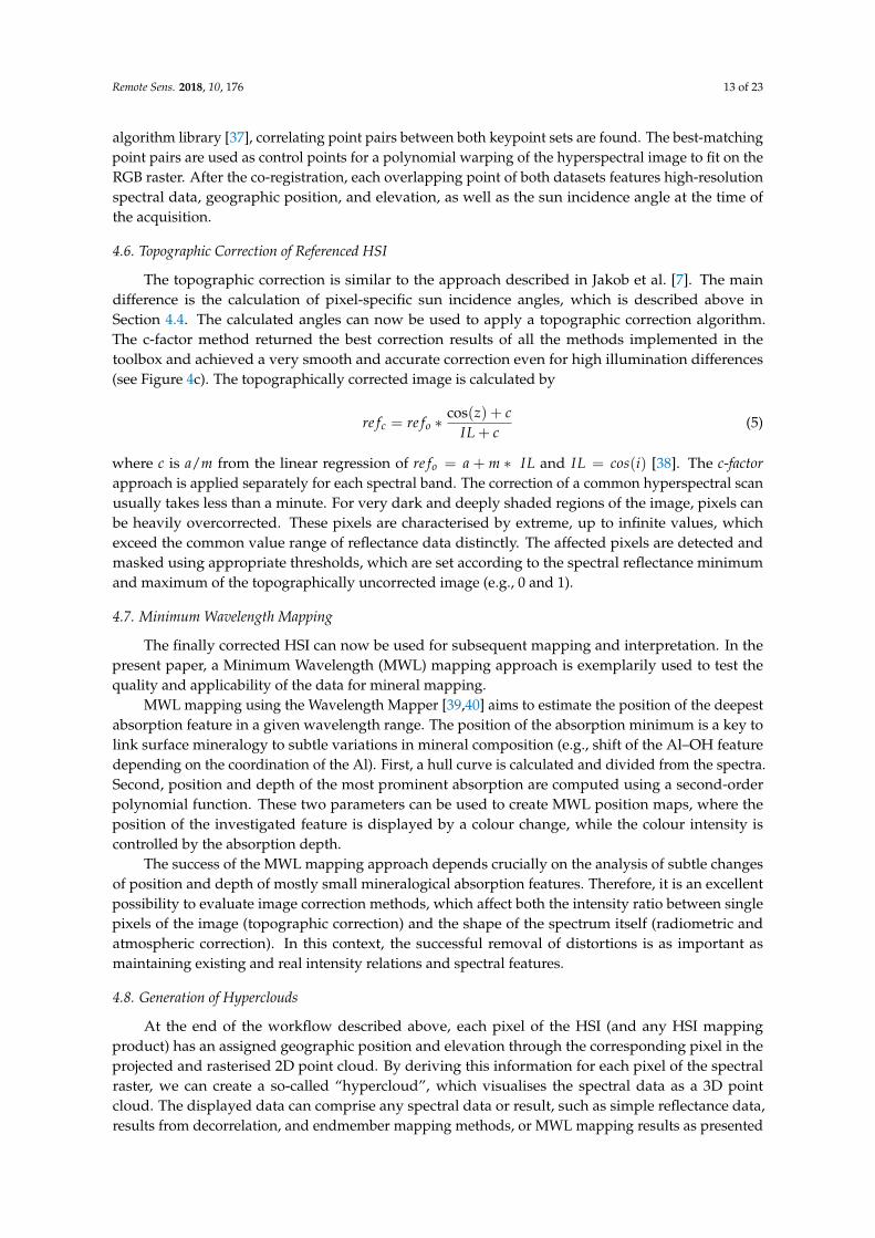
Two hyperspectral scans were acquired from two different scanning locations, covering thelargest part of the south and east coast of the Nunngarut Peninsula (Figure 1a). The approximatedistance between sensor and observed target ranged between 2 and 5 km for the majority of alloutcrop-related image pixels. Despite overall dry and sunny conditions during acquisition, numeroussharp atmospheric absorption features within the spectral data (see Figures 3 and 7) suggested ahigh influence of the atmospheric layer between the sensor and the target. Figure 7 displays theknown major atmospheric contributions (in this case water vapour, CO2, O2, and O3) to the overallobserved atmospheric perturbances and the resulting calculated spectrum used for the corrections.We showcase that the radiometric correction approach presented here allows us to remove theinfluence of the atmosphere almost completely, whereas typical mineral-related spectral featuresof the Mârmorilik Formation remain. In the resulting atmospherically corrected target spectrum,the remaining absorption features are indubitably attributable to characteristic mineral features.Besides the distinct carbonate feature of the Mârmorilik marbles, the characteristic AlOH and OH/H2Ofeatures are clearly represented. These characteristic absorptions are related either to abundantevaporitic gypsum and/or clay minerals originating from inclusions or nearby pelite horizons knownto be present in this lithological unit.

Scan 1, imaging the south facing cliff of the Nunngarut Peninsula, was directly opposed to thesun during the measurements and is therefore evenly illuminated. In contrast, Scan 2, acquired in themorning and facing the eastern coast of the peninsula, featured high illumination differences, whichmade a topographic correction crucial for the subsequent mapping process (Figure 4c).

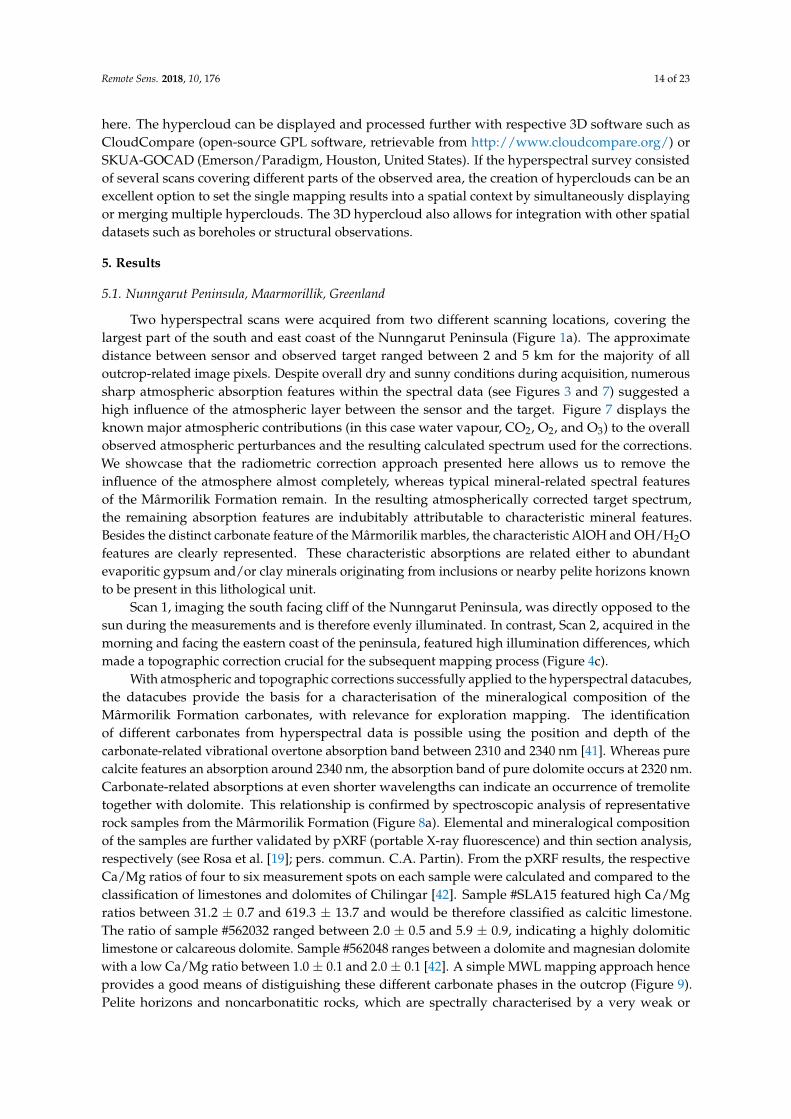
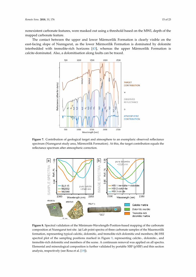
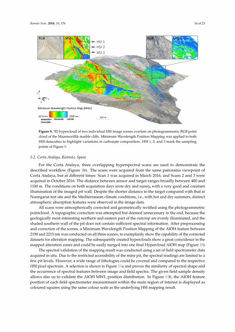
With atmospheric and topographic corrections successfully applied to the hyperspectral datacubes,the datacubes provide the basis for a characterisation of the mineralogical composition of theMârmorilik Formation carbonates, with relevance for exploration mapping. The identificationof different carbonates from hyperspectral data is possible using the position and depth of thecarbonate-related vibrational overtone absorption band between 2310 and 2340 nm [41]. Whereas purecalcite features an absorption around 2340 nm, the absorption band of pure dolomite occurs at 2320 nm.Carbonate-related absorptions at even shorter wavelengths can indicate an occurrence of tremolitetogether with dolomite. This relationship is confirmed by spectroscopic analysis of representativerock samples from the Mârmorilik Formation (Figure 8a). Elemental and mineralogical compositionof the samples are further validated by pXRF (portable X-ray fluorescence) and thin section analysis,respectively (see Rosa et al. [19]; pers. commun. C.A. Partin). From the pXRF results, the respectiveCa/Mg ratios of four to six measurement spots on each sample were calculated and compared to theclassification of limestones and dolomites of Chilingar [42]. Sample #SLA15 featured high Ca/Mgratios between 31.2 ± 0.7 and 619.3 ± 13.7 and would be therefore classified as calcitic limestone.The ratio of sample #562032 ranged between 2.0 ± 0.5 and 5.9 ± 0.9, indicating a highly dolomiticlimestone or calcareous dolomite. Sample #562048 ranges between a dolomite and magnesian dolomitewith a low Ca/Mg ratio between 1.0 ± 0.1 and 2.0 ± 0.1 [42]. A simple MWL mapping approach henceprovides a good means of distiguishing these different carbonate phases in the outcrop (Figure 9).Pelite horizons and noncarbonatitic rocks, which are spectrally characterised by a very weak or

Remote Sens. 2018, 10, 176 15 of 23

nonexistent carbonate features, were masked out using a threshold based on the MWL depth of themapped carbonate feature.

The contact between the upper and lower Mârmorilik Formation is clearly visible on theeast-facing slope of Nunngarut, as the lower Mârmorilik Formation is dominated by dolomiteinterbedded with tremolite-rich horizons [43], whereas the upper Mârmorilik Formation iscalcite-dominated. Also, a dolomitisation along faults can be traced.Remote Sens. 2018, 10, x FOR PEER REVIEW 15 of 23

Figure 7. Contribution of geological target and atmosphere to an exemplaric observed reflectance spectrum (Nunngarut study area, Mârmorilik Formation). At this, the target contribution equals the reflectance spectrum after atmospheric correction.

Figure 8. Spectral validation of the Minimum-Wavelength-Position-based mapping of the carbonate composition at Nunngarut test site. (a) Lab point spectra of three carbonate samples of the Maarmorilik formation, representing typical calcitic, dolomitic, and tremolite-rich dolomitic end members; (b) HSI spectral plot of the sampling positions marked in Figure 9, representing calcite-, dolomite-, and tremolite-rich dolomitic end members of the scene. A continuum removal was applied on all spectra. Elemental and mineralogical composition is further validated by portable XRF (pXRF) and thin section analysis, respectively (see Rosa et al. [19]).

Figure 7. Contribution of geological target and atmosphere to an exemplaric observed reflectancespectrum (Nunngarut study area, Mârmorilik Formation). At this, the target contribution equals thereflectance spectrum after atmospheric correction.

Remote Sens. 2018, 10, x FOR PEER REVIEW 15 of 23

Figure 7. Contribution of geological target and atmosphere to an exemplaric observed reflectance spectrum (Nunngarut study area, Mârmorilik Formation). At this, the target contribution equals the reflectance spectrum after atmospheric correction.

Figure 8. Spectral validation of the Minimum-Wavelength-Position-based mapping of the carbonate composition at Nunngarut test site. (a) Lab point spectra of three carbonate samples of the Maarmorilik formation, representing typical calcitic, dolomitic, and tremolite-rich dolomitic end members; (b) HSI spectral plot of the sampling positions marked in Figure 9, representing calcite-, dolomite-, and tremolite-rich dolomitic end members of the scene. A continuum removal was applied on all spectra. Elemental and mineralogical composition is further validated by portable XRF (pXRF) and thin section analysis, respectively (see Rosa et al. [19]).

Figure 8. Spectral validation of the Minimum-Wavelength-Position-based mapping of the carbonatecomposition at Nunngarut test site. (a) Lab point spectra of three carbonate samples of the Maarmorilikformation, representing typical calcitic, dolomitic, and tremolite-rich dolomitic end members; (b) HSIspectral plot of the sampling positions marked in Figure 9, representing calcite-, dolomite-, andtremolite-rich dolomitic end members of the scene. A continuum removal was applied on all spectra.Elemental and mineralogical composition is further validated by portable XRF (pXRF) and thin sectionanalysis, respectively (see Rosa et al. [19]).

Remote Sens. 2018, 10, 176 16 of 23Remote Sens. 2018, 10, x FOR PEER REVIEW 16 of 23

Figure 9. 3D hypercloud of two individual HSI image scenes overlain on photogrammetric RGB point cloud of the Maarmorillik marble cliffs. Minimum Wavelength Position Mapping was applied to both HSI datacubes to highlight variations in carbonate composition. HSI 1, 2, and 3 mark the sampling points of Figure 8.

5.2. Corta Atalaya, Riotinto, Spain

For the Corta Atalaya, three overlapping hyperspectral scans are used to demonstrate the described workflow (Figure 1b). The scans were acquired from the same panorama viewpoint of Corta Atalaya, but at different times: Scan 1 was acquired in March 2016, and Scans 2 and 3 were acquired in October 2016. The distance between sensor and target ranges broadly between 400 and 1100 m. The conditions on both acquisition days were dry and sunny, with a very good and constant illumination of the imaged pit wall. Despite the shorter distance to the target compared with that at Nunngarut test site and the Mediterranean climate conditions, i.e., with hot and dry summers, distinct atmospheric absorption features were observed in the image data.

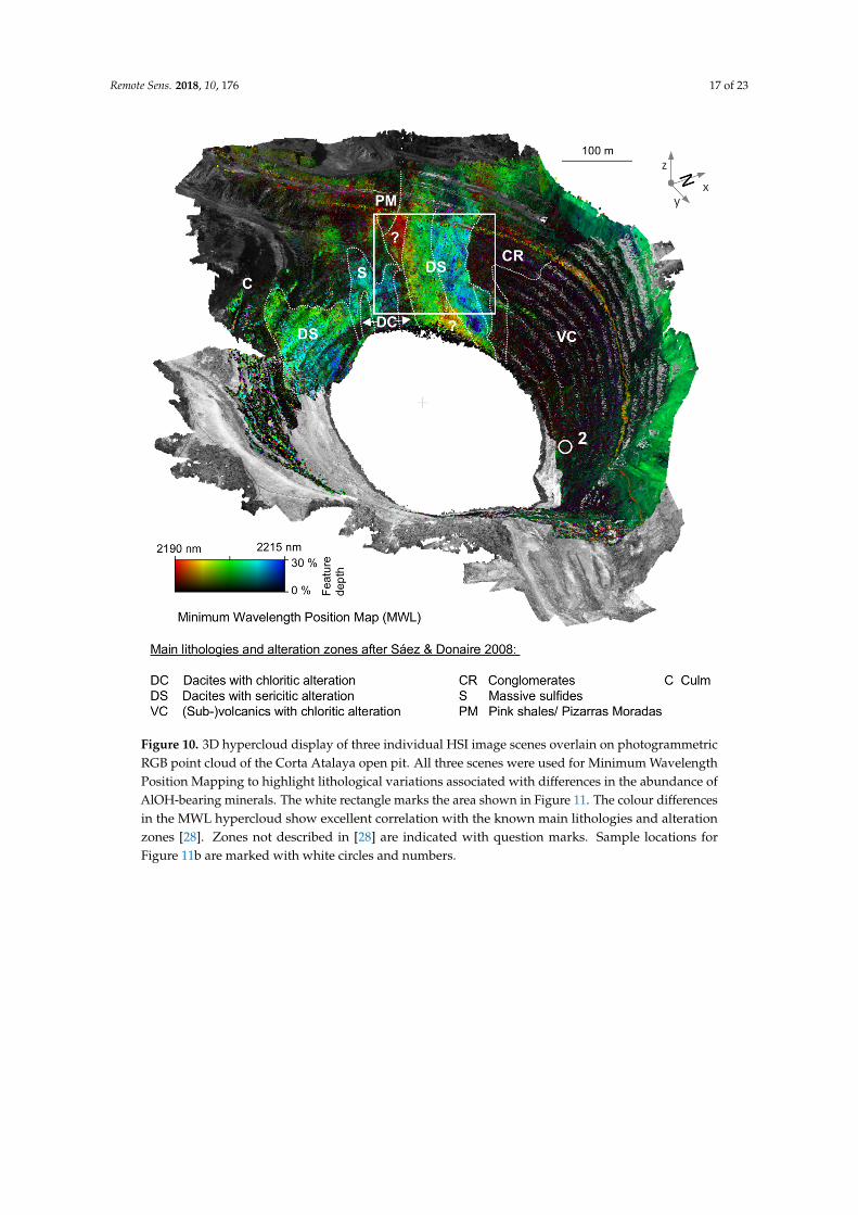
All scans were atmospherically corrected and geometrically rectified using the photogrammetric pointcloud. A topographic correction was attempted but deemed unnecessary in the end, because the geologically most interesting northern and eastern part of the outcrop are evenly illuminated, and the shaded southern wall of the pit does not contain sufficient spectral information. After preprocessing and correction of the scenes, a Minimum Wavelength Position Mapping of the AlOH feature between 2190 and 2215 nm was conducted on all three scenes, to exemplarily show the capability of the corrected datasets for alteration mapping. The subsequently created hyperclouds show a great coincidence in the mapped alteration zones and could be easily merged into one final Hypercloud AlOH map (Figure 10).

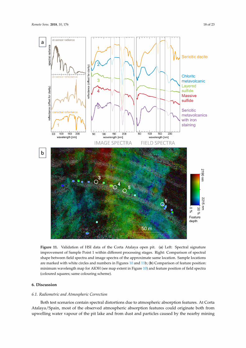
The spectral validation of the mapping result was conducted using a set of field spectrometer data acquired in situ. Due to the restricted accessibility of the mine pit, the spectral readings are limited to a few pit levels. However, a wide range of lithologies could be covered and compared to the respective HSI pixel spectrum. A selection is shown in Figure 11a and proves the similarity of spectral shape and the occurrence of spectral features between image and field spectra. The given field sample density allows also us to validate the AlOH MWL position distribution. In Figure 11b, the AlOH feature position of each field spectrometer measurement within the main region of interest is displayed as coloured squares using the same colour scale as the underlying HSI mapping result.

Figure 9. 3D hypercloud of two individual HSI image scenes overlain on photogrammetric RGB pointcloud of the Maarmorillik marble cliffs. Minimum Wavelength Position Mapping was applied to bothHSI datacubes to highlight variations in carbonate composition. HSI 1, 2, and 3 mark the samplingpoints of Figure 8.

5.2. Corta Atalaya, Riotinto, Spain

For the Corta Atalaya, three overlapping hyperspectral scans are used to demonstrate thedescribed workflow (Figure 1b). The scans were acquired from the same panorama viewpoint ofCorta Atalaya, but at different times: Scan 1 was acquired in March 2016, and Scans 2 and 3 wereacquired in October 2016. The distance between sensor and target ranges broadly between 400 and1100 m. The conditions on both acquisition days were dry and sunny, with a very good and constantillumination of the imaged pit wall. Despite the shorter distance to the target compared with that atNunngarut test site and the Mediterranean climate conditions, i.e., with hot and dry summers, distinctatmospheric absorption features were observed in the image data.

All scans were atmospherically corrected and geometrically rectified using the photogrammetricpointcloud. A topographic correction was attempted but deemed unnecessary in the end, because thegeologically most interesting northern and eastern part of the outcrop are evenly illuminated, and theshaded southern wall of the pit does not contain sufficient spectral information. After preprocessingand correction of the scenes, a Minimum Wavelength Position Mapping of the AlOH feature between2190 and 2215 nm was conducted on all three scenes, to exemplarily show the capability of the correcteddatasets for alteration mapping. The subsequently created hyperclouds show a great coincidence in themapped alteration zones and could be easily merged into one final Hypercloud AlOH map (Figure 10).

The spectral validation of the mapping result was conducted using a set of field spectrometer dataacquired in situ. Due to the restricted accessibility of the mine pit, the spectral readings are limited to afew pit levels. However, a wide range of lithologies could be covered and compared to the respectiveHSI pixel spectrum. A selection is shown in Figure 11a and proves the similarity of spectral shape andthe occurrence of spectral features between image and field spectra. The given field sample densityallows also us to validate the AlOH MWL position distribution. In Figure 11b, the AlOH featureposition of each field spectrometer measurement within the main region of interest is displayed ascoloured squares using the same colour scale as the underlying HSI mapping result.

Remote Sens. 2018, 10, 176 17 of 23Remote Sens. 2018, 10, x FOR PEER REVIEW 17 of 23

Figure 10. 3D hypercloud display of three individual HSI image scenes overlain on photogrammetric RGB point cloud of the Corta Atalaya open pit. All three scenes were used for Minimum Wavelength Position Mapping to highlight lithological variations associated with differences in the abundance of AlOH-bearing minerals. The white rectangle marks the area shown in Figure 11. The colour differences in the MWL hypercloud show excellent correlation with the known main lithologies and alteration zones [28]. Zones not described in [28] are indicated with question marks. Sample locations for Figure 11b are marked with white circles and numbers.

Figure 10. 3D hypercloud display of three individual HSI image scenes overlain on photogrammetricRGB point cloud of the Corta Atalaya open pit. All three scenes were used for Minimum WavelengthPosition Mapping to highlight lithological variations associated with differences in the abundance ofAlOH-bearing minerals. The white rectangle marks the area shown in Figure 11. The colour differencesin the MWL hypercloud show excellent correlation with the known main lithologies and alterationzones [28]. Zones not described in [28] are indicated with question marks. Sample locations forFigure 11b are marked with white circles and numbers.

Remote Sens. 2018, 10, 176 18 of 23Remote Sens. 2018, 10, x FOR PEER REVIEW 18 of 23

Figure 11. Validation of HSI data of the Corta Atalaya open pit. (a) Left: Spectral signature improvement of Sample Point 1 within different processing stages. Right: Comparison of spectral shape between field spectra and image spectra of the approximate same location. Sample locations are marked with white circles and numbers in Figures 10 and 11b; (b) Comparison of feature position: minimum wavelength map for AlOH (see map extent in Figure 10) and feature position of field spectra (coloured squares; same colouring scheme).

6. Discussion

6.1. Radiometric and Atmospheric Correction

Both test scenarios contain spectral distortions due to atmospheric absorption features. At Corta Atalaya/Spain, most of the observed atmospheric absorption features could originate both from upwelling water vapour of the pit lake and from dust and particles caused by the nearby mining

Figure 11. Validation of HSI data of the Corta Atalaya open pit. (a) Left: Spectral signatureimprovement of Sample Point 1 within different processing stages. Right: Comparison of spectralshape between field spectra and image spectra of the approximate same location. Sample locationsare marked with white circles and numbers in Figures 10 and 11b; (b) Comparison of feature position:minimum wavelength map for AlOH (see map extent in Figure 10) and feature position of field spectra(coloured squares; same colouring scheme).

6. Discussion

6.1. Radiometric and Atmospheric Correction

Both test scenarios contain spectral distortions due to atmospheric absorption features. At CortaAtalaya/Spain, most of the observed atmospheric absorption features could originate both fromupwelling water vapour of the pit lake and from dust and particles caused by the nearby mining

Remote Sens. 2018, 10, 176 19 of 23

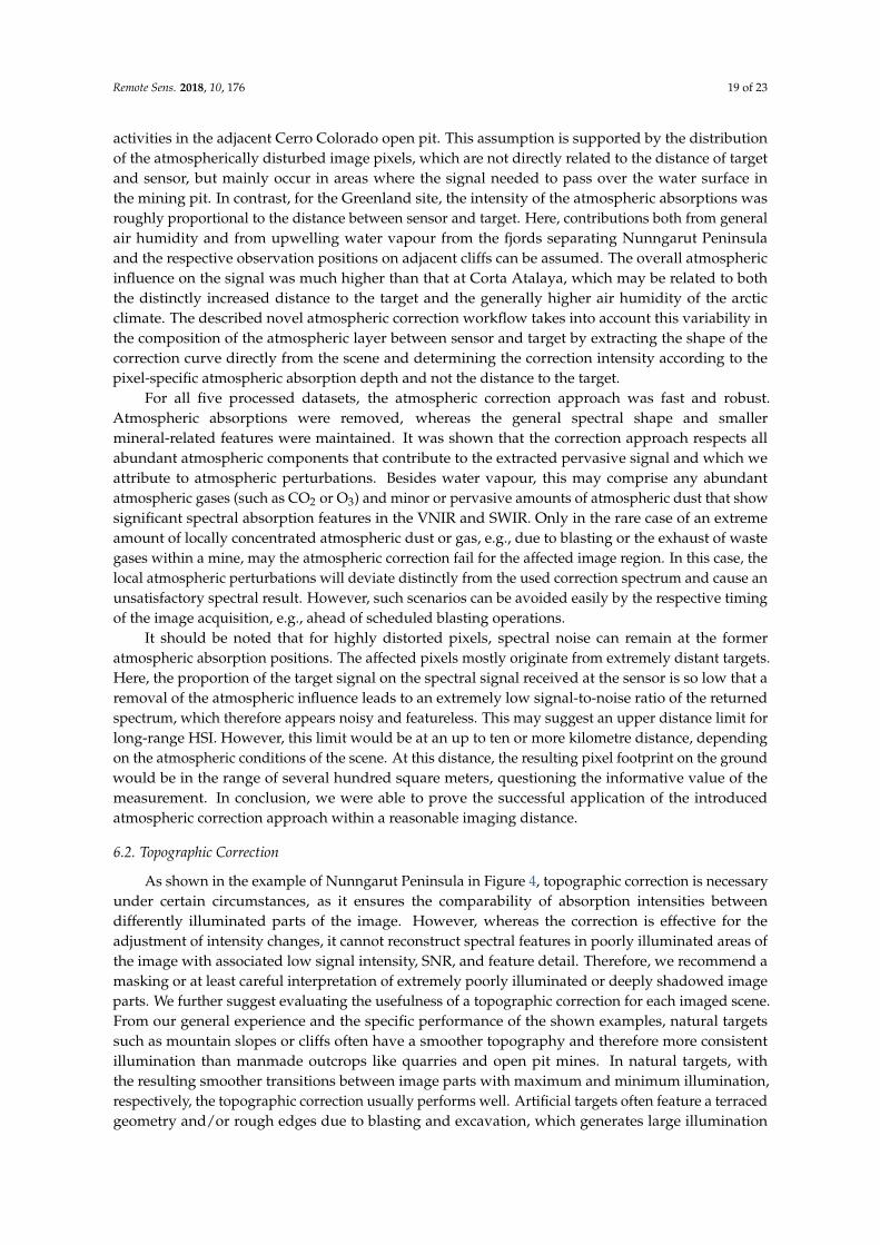
activities in the adjacent Cerro Colorado open pit. This assumption is supported by the distributionof the atmospherically disturbed image pixels, which are not directly related to the distance of targetand sensor, but mainly occur in areas where the signal needed to pass over the water surface inthe mining pit. In contrast, for the Greenland site, the intensity of the atmospheric absorptions wasroughly proportional to the distance between sensor and target. Here, contributions both from generalair humidity and from upwelling water vapour from the fjords separating Nunngarut Peninsulaand the respective observation positions on adjacent cliffs can be assumed. The overall atmosphericinfluence on the signal was much higher than that at Corta Atalaya, which may be related to boththe distinctly increased distance to the target and the generally higher air humidity of the arcticclimate. The described novel atmospheric correction workflow takes into account this variability inthe composition of the atmospheric layer between sensor and target by extracting the shape of thecorrection curve directly from the scene and determining the correction intensity according to thepixel-specific atmospheric absorption depth and not the distance to the target.

For all five processed datasets, the atmospheric correction approach was fast and robust.Atmospheric absorptions were removed, whereas the general spectral shape and smallermineral-related features were maintained. It was shown that the correction approach respects allabundant atmospheric components that contribute to the extracted pervasive signal and which weattribute to atmospheric perturbations. Besides water vapour, this may comprise any abundantatmospheric gases (such as CO2 or O3) and minor or pervasive amounts of atmospheric dust that showsignificant spectral absorption features in the VNIR and SWIR. Only in the rare case of an extremeamount of locally concentrated atmospheric dust or gas, e.g., due to blasting or the exhaust of wastegases within a mine, may the atmospheric correction fail for the affected image region. In this case, thelocal atmospheric perturbations will deviate distinctly from the used correction spectrum and cause anunsatisfactory spectral result. However, such scenarios can be avoided easily by the respective timingof the image acquisition, e.g., ahead of scheduled blasting operations.

It should be noted that for highly distorted pixels, spectral noise can remain at the formeratmospheric absorption positions. The affected pixels mostly originate from extremely distant targets.Here, the proportion of the target signal on the spectral signal received at the sensor is so low that aremoval of the atmospheric influence leads to an extremely low signal-to-noise ratio of the returnedspectrum, which therefore appears noisy and featureless. This may suggest an upper distance limit forlong-range HSI. However, this limit would be at an up to ten or more kilometre distance, dependingon the atmospheric conditions of the scene. At this distance, the resulting pixel footprint on the groundwould be in the range of several hundred square meters, questioning the informative value of themeasurement. In conclusion, we were able to prove the successful application of the introducedatmospheric correction approach within a reasonable imaging distance.

6.2. Topographic Correction

As shown in the example of Nunngarut Peninsula in Figure 4, topographic correction is necessaryunder certain circumstances, as it ensures the comparability of absorption intensities betweendifferently illuminated parts of the image. However, whereas the correction is effective for theadjustment of intensity changes, it cannot reconstruct spectral features in poorly illuminated areas ofthe image with associated low signal intensity, SNR, and feature detail. Therefore, we recommend amasking or at least careful interpretation of extremely poorly illuminated or deeply shadowed imageparts. We further suggest evaluating the usefulness of a topographic correction for each imaged scene.From our general experience and the specific performance of the shown examples, natural targetssuch as mountain slopes or cliffs often have a smoother topography and therefore more consistentillumination than manmade outcrops like quarries and open pit mines. In natural targets, withthe resulting smoother transitions between image parts with maximum and minimum illumination,respectively, the topographic correction usually performs well. Artificial targets often feature a terracedgeometry and/or rough edges due to blasting and excavation, which generates large illumination

Remote Sens. 2018, 10, 176 20 of 23

differences. A topographic correction will not necessarily give an improvement of the image, as theapplied corrections in the well-illuminated parts are minor, while the correction of the dark parts maybe futile due to the mentioned reasons.

The c-factor method, despite its good performance for topographic correction, needs to be appliedcarefully. Due to the bandwise calculation of the correction factor using a linear regression, extremeor infinite values in one or several bands can cause an exaggeration of the correction factor for thosebands and, finally, a change in the spectral shape. These peak values can be caused by bad pixelsin the HSI sensor, which, due to the push-broom character of the camera, form bad pixel lines thatare restricted to few adjacent bands. If a topographic correction needs to be applied, a correction ormasking of those bad lines is inevitably required for a reliable image result.

6.3. Validation

The spectral validation using field spectrometer data demonstrated a great accuracy of bothspectral shape and feature position of the corrected image spectra. In general, the difference betweenthe interpolated minimum wavelength of field spectra and the corresponding library spectra for acertain absorption feature was below 5 nm in both areas of investigation. This value represents theband sampling distance of the SWIR data and lies below the achievable spectral resolution of 12 nm(FWHM). Locally, higher errors between some image and validation spectra points were observed,but these may be related to the large difference in spatial footprints of the different instruments.The field spectrometer data were retrieved from one or several 8 mm spots of a single lithologicallyrepresentative sample, whereas the respective HSI pixel can easily represent a mixture of an area ofsome square meters of outcrop, depending on the distance to the sensor. Local variability in alterationcan affect the representability of the spectrometer reading and lead to deviations from the recordedimage spectrum at the same location. Additional to the spectral variations, slight mislocation of thespectrometer readings, which can be caused by the limited accuracy of the sample GPS position thatcan reach up to 5 m, needs to be taken into account.

6.4. 3D Integration

The potential, the spatial accuracy, and a possible application of the HSI integration withphotogrammetric point clouds is discussed in more detail in Salehi et al. [20]. The current paperconfirms not only the successful 3D integration for two additional examples, but further provesthe capability of the workflow to integrate and merge hyperspectral datasets from different cameralocations and viewing angles as well as different acquisition dates and times by eliminating the effectsof topography, different illumination conditions, and atmospheric absorptions. This allows the useof hyperspectral data in a new way, as it facilitates the evaluation of spatial relationships betweenhyperspectral results that are not visible from one observation point or displayable in one dataset, suchas opposing faces of a mountain or a mining pit.

7. Conclusions

With this paper, we present a novel approach for the atmospheric and topographic correction oflong-range ground-based hyperspectral imagery. Such corrections are essential for obtaining reliableinformation on mineral composition in geological applications. The general workflow is partly basedon the algorithms developed for drone-borne and vessel-based HSI data, which were presented andused in our previous papers [7,20], but is adapted and extended by adding radiometric and topographiccorrection approaches to meet the particular challenges of long-range, ground-based HSI.

The most important outcomes of this paper are the following:

1. The correction spectrum for the atmospheric correction is derived directly from the scene, andthe correction intensity is determined according to the pixel-specific atmospheric absorption

Remote Sens. 2018, 10, 176 21 of 23

depth. As a result, the workflow is independent from knowledge about the composition of theatmospheric layer or the distance to the target.

2. The incidence angles for the topographic corrections are calculated using the point normals ofthe photogrammetric 3D outcrop model. This allows us, for the first time, to utilise commontopographic correction algorithms, such as the used c-factor method, for vertical outcrops.

3. The generation of a hypercloud, i.e., a geometrically and spectrally accurate combination ofa photogrammetric point cloud and the HSI datacube, is achieved through the projectivetransformations of a photogrammetric 3D outcrop model. The removal of the effects ofatmosphere and topography allows the integration of hyperspectral mapping results originatingfrom different camera positions, dates, and, therefore, varying illumination conditions.

4. Two study areas with five HSI datasets in total proved the applicability and robustness ofthe workflow in differently challenging measuring conditions regarding climate, distance,atmospheric composition, geological diversity, and mapping objectives. A successful MWLmapping demonstrated both the geological applicability and the accuracy of spectral absorptionpositions and depths.

5. The accuracy and reliability of the created data and mapping results is validated by field spectraand the mineralogical analysis of geological samples.

6. The presented workflow is fast and simple and requires only a minimum of input parameters.Most of the processing steps are automatised and need no or extremely few manual actions.

7. The workflow enables (i) reliable spectral mapping of vertical and completely inaccessibleoutcrops; (ii) three-dimensional integration of multiple scans and other data sources; and (iii) ahigher spectral resolution, range, and SNR than most drone- or air-borne HSI data.

On account of the promising quality of the presented datasets, we highly encourage the use ofcarefully processed and corrected long-range ground-based HSI data for geological applications andsuggest a further development of highly adapted topographic and atmospheric correction algorithms.In several upcoming application-based papers, we will further present and discuss the geologicalinterpretation of data corrected with the presented workflow and their integration with other datatypes such as structural data and long-wave infrared (LWIR) hyperspectral data.

Acknowledgments: The Helmholtz Institute Freiberg for Resource Technology is gratefully thanked forsupporting and funding this project. The authors thank the entire group of “Exploration Technology” for theirconstructive feedback and extensive testing of the scripts. Further, we thank Atalaya Mining for access to Riotintomine and IPH Ingeniería y proyectos for performing the UAS flight in Corta Atalaya. The Ministry for MineralResources, Government of Greenland, and the Geological Survey of Denmark and Greenland are gratefullyacknowledged for funding and supporting fieldwork and data acquisition within the project “Karrat Zinc”.

Author Contributions: S.L. developed the processing workflow with substantial contributions from S.S., M.K.,and R.G. and implemented the workflow in Python. R.Z. and E.V.S. delivered logistic support in the field and wereresponsible for data acquisition and photogrammetric processing. S.L., R.Z., and G.U. processed the hyperspectraldatasets and performed the geological interpretation and validation. S.L. wrote the manuscript with input fromall authors. R.G. supervised the study at all stages.

Conflicts of Interest: The authors declare no conflict of interest.

References

1. Hubbard, B.E.; Crowley, C.K.; Zimbelman, D.R. Comparative alteration mineral mapping using visible toshortwave infrared (0.4–2.4 mm) Hyperion, ALI, and ASTER imagery. IEEE Trans. Geosci. Remote Sens. 2003,41, 1401–1410. [CrossRef]

2. Kruse, F.A. Mineral mapping with AVIRIS and EO-1 Hyperion. In Proceedings of the 12th JPL AirborneGeoscience Workshop; Pasadena, CA, USA, 24–28 January 2003, Jet Propulsion Laboratory: Pasadena, CA,USA, 2003; Volume 41, pp. 149–156.

3. Bedini, E. Mapping lithology of the Sarfartoq carbonatite complex, southern West Greenland, using HyMapimaging spectrometer data. Remote Sens. Environ. 2009, 113, 1208–1219. [CrossRef]

Remote Sens. 2018, 10, 176 22 of 23

4. Laukamp, C.; Cudahy, T.; Thomas, M.; Jones, M.; Cleverley, J.S.; Oliver, N.H. Hydrothermal mineral alterationpatterns in the Mount Isa Inlier revealed by airborne hyperspectral data. Aust. J. Earth Sci. 2011, 58, 917–936.[CrossRef]

5. Zimmermann, R.; Brandmeier, M.; Andreani, L.; Mhopjeni, K.; Gloaguen, R. Remote Sensing Exploration ofNb-Ta-LREE-Enriched Carbonatite (Epembe/Namibia). Remote Sens. 2016, 8, 620. [CrossRef]

6. Jakob, S.; Gloaguen, R.; Laukamp, C. Remote Sensing-Based Exploration of Structurally-RelatedMineralizations around Mount Isa, Queensland, Australia. Remote Sens. 2016, 8, 358. [CrossRef]

7. Jakob, S.; Zimmermann, R.; Gloaguen, R. The Need for Accurate Geometric and Radiometric Correctionsof Drone-Borne Hyperspectral Data for Mineral Exploration: MEPHySTo—A Toolbox for Pre-ProcessingDrone-Borne Hyperspectral Data. Remote Sens. 2017, 9, 88. [CrossRef]

8. Gao, B.-C.; Heidebrecht, K.B.; Goetz, A.F.H. Derivation of scaled surface reflectances from AVIRIS data.Remote Sens. Environ. 1993, 44, 165–178. [CrossRef]

9. Adler-Golden, S.M.; Matthew, W.M.; Bernstein, L.S.; Levine, R.Y.; Berk, A.; Richtsmeier, S.C.; Acharya, P.K.;Anderson, G.P.; Felde, J.W.; Gardner, J.A.; et al. Atmospheric correction for shortwave spectral imagery basedon MODTRAN4. In Summaries of the Eighth JPL Airborne Earth Science Workshop; Jet Propulsion Laboratory:Pasadena, CA, USA, 1999; Volume 99–17, pp. 21–29.

10. Richter, R.; Schlaepfer, D. Geo-atmospheric processing of airborne imaging spectrometry data, Part 2:Atmospheric/topographic correction. Int. J. Remote Sens. 2002, 23, 2631–2649. [CrossRef]

11. Smith, G.M.; Milton, E.J. The use of the empirical line method to calibrate remotely sensed data to reflectance.Int. J. Remote Sens. 1999, 20, 2653–2662. [CrossRef]

12. Roberts, D.A.; Yamaguchi, Y.; Lyon, R. Comparison of various techniques for calibration of AIS data.In Proceedings of the 2nd Airborne Imaging Spectrometer Data Analysis Workshop; Pasadena, CA, USA,6–8 May 1986; Jet Propulsion Laboratory: Pasadena, CA, USA, 1986; Volume 86–35, pp. 21–30.

13. Chavez, P.S. An improved dark-object subtraction technique for atmospheric scattering correction ofmultispectral data. Remote Sens. Environ. 1988, 24, 459–479. [CrossRef]

14. Clark, R.N.; Swayze, G.A.; Livo, K.E.; Kokaly, R.F.; King, T.V.V.; Dalton, J.B.; Vance, J.S.; Rockwell, B.W.;Hoefen, T.; McDougal, R.R. Surface Reflectance Calibration of Terrestrial Imaging Spectroscopy Data:A Tutorial Using AVIRIS. In Proceedings of the 10th Airborne Earth Science Workshop; Jet Propulsion Laboratory:Pasadena, CA, USA, 2002; Volume 02-1.

15. Laliberte, A.S.; Goforth, M.A.; Steele, C.M.; Rango, A. Multispectral remote sensing from unmanned aircraft:Image processing workflows and applications for rangeland environments. Remote Sens. 2011, 3, 2529–2551.[CrossRef]

16. Kurz, T.H.; Buckley, S.J.; Howell, J.A. Close-range hyperspectral imaging for geological field studies:Workflow and methods. Int. J. Remote Sens. 2013, 34, 1798–1822. [CrossRef]

17. Kurz, T.H.; Buckley, S.J. A review of hyperspectral imaging in close range applications. Int. Arch. Photogramm.Remote Sens. Spat. Inf. Sci. 2016, 41, 865–870. [CrossRef]

18. Murphy, R.J.; Taylor, Z.; Schneider, S.; Nieto, J. Mapping clay minerals in an open-pit mine usinghyperspectral and LiDAR data. Eur. J. Remote Sens. 2015, 48, 511–526. [CrossRef]

19. Rosa, D.; Dewolfe, M.; Guarnieri, P.; Kolb, J.; Laflamme, C.; Partin, C.A.; Salehi, S.; Sørensen, E.V.; Thaarup, S.;Thrane, K.; et al. Architecture and Mineral Potential of the Paleoproterozoic Karrat Group, West Greenland: Resultsof the 2016 Season; GEUS Rapport 2017/5; Geological Survey of Denmark and Greenland: Copenhagen,Denmark, 2017; p. 112.

20. Salehi, S.; Lorenz, S.; Sørensen, E.V.; Zimmermann, R.; Fensholt, R.; Heincke, B.H.; Kirsch, M.; Gloaguen, R.Integration of Vessel-Based Hyperspectral Scanning and 3D-Photogrammetry for Mobile Mapping of SteepCoastal Cliffs in the Arctic. Remote Sens. 2008, 10, 175. [CrossRef]

21. Kolb, J.; Keiding, J.K.; Steenfeld, A.; Secher, K.; Keulen, N.; Rosa, D.; Stensgaard, B. M Metallogeny ofGreenland. Ore Geol. Rev. 2016, 78, 493–555. [CrossRef]

22. Sørensen, L.L.; Stensgaard, B.M.; Thrane, K.; Rosa, D.; Kalvig, P. Sediment-Hosted Zinc Potential in Greenland;GEUS Rapport 2013/56; Geological Survey of Denmark and Greenland: Copenhagen, Denmark, 2013; p. 184.

23. Grocott, J.; McCaffrey, K.J.W. Basin evolution and destruction in an Early Proterozoic continental margin:The Rinkian fold–thrust belt of central West Greenland. J. Geol. Soc. 2017, 174, 453–467. [CrossRef]

24. Pedersen, F.D. Remobilization of the massive sulfide ore of the Black Angel Mine, central West Greenland.Econ. Geol. 1980, 75, 1022–1041. [CrossRef]

Remote Sens. 2018, 10, 176 23 of 23

25. Henderson, G.; Pulvertaft, T.C.R. Geological Map of Greenland, 1:100 000. Mârmorilik 71 V.2 Syd, Nûgâtsiaq 71V.2 Nord, Pangnertôq 72 V.2 Syd. Lithostratigraphy and Structure of a Lower Proterozoic Dome and Nappe Complex;Geological Survey of Greenland: Copenhagen, Denmark, 1987; p. 72.

26. Guarnieri, P.; Partin, C.; Rosa, D. Palaeovalleys at the Basal Unconformity of the Palaeoproterozoic Karrat Group,West Greenland; Geological Survey of Denmark and Greenland Bulletin; Geological Survey of Denmark andGreenland: Copenhagen, Denmark, 2016; pp. 63–66.

27. Rosa, D.; Guarnieri, P.; Hollis, J.; Kolb, J.; Partin, C.A.; Petersen, J.; Sørensen, E.V.; Thomassen, B.; Thomsen, L.;Thrane, K. Architecture and Mineral Potential of the Paleoproterozoic Karrat Group, West Greenland: Results of the2015 Season; Geological Survey of Denmark and Greenland: Copenhagen, Denmark, 2016; p. 98.

28. Sáez, R.; Donaire, T. Corta atalaya. In Geología de Huelva: Lugares de Interés Geológico; Universidad de Huelva,Facultad de Ciencias Experimentales: Huelva, Spain, 2008; pp. 106–111.

29. Soriano, C.; Casas, J. Variscan tectonics in the Iberian Pyrite Belt, South Portuguese Zone. Int. J. Earth Sci.2002, 91, 882–896. [CrossRef]

30. Green, A.A.; Berman, M.; Switzer, P.; Craig, M.D. A transformation for ordering multispectral data in termsof image quality with implications for noise removal. IEEE Trans. Geosci. Remote Sens. 1988, 26, 65–74.[CrossRef]

31. Phillips, R.D.; Blinn, C.E.; Watson, L.T.; Wynne, R.H. An Adaptive Noise-Filtering Algorithm for AVIRISData with Implications for Classification Accuracy. IEEE Trans. Geosci. Remote Sens. 2009, 47, 3168–3179.[CrossRef]

32. Westoby, M.J.; Brasington, J.; Glasser, N.F.; Hambrey, M.J.; Reynolds, J.M. ‘Structure-from-Motion’photogrammetry: A low-cost, effective tool for geoscience applications. Geomorphology 2012, 179, 300–314.[CrossRef]

33. Eltner, A.; Kaiser, A.; Castillo, C.; Rock, G.; Neugirg, F.; Abellán, A. Image-based surface reconstruction ingeomorphometry—Merits, limits and developments. Earth Surf. Dyn. 2016, 4, 359–389. [CrossRef]

34. Carrivick, J.L.; Smith, M.W.; Quincey, D.J. Structure from Motion in the Geosciences; John Wiley & Sons, Ltd.:Chichester, UK, 2016; ISBN 978-1-118-89581-8.

35. James, M.R.; Robson, S.; d’Oleire-Oltmanns, S.; Niethammer, U. Optimising UAV topographic surveysprocessed with structure-from-motion: Ground control quality, quantity and bundle adjustment.Geomorphology 2017, 280, 51–66. [CrossRef]

36. Lowe, D.G. Object recognition from local scale-invariant features. In Proceedings of the InternationalConference on Computer Vision, Kerkyra, Greece, 20–27 September 1999; Volume 2, pp. 1150–1157.

37. Muja, M.; Lowe, D. Fast approximate nearest neighbors with automatic algorithm configuration.In Proceedings of the Fourth International Conference on Computer Vision Theory and Applications,Lisboa, Portugal, 5–8 February 2009; Volume 1, pp. 1–10.

38. Teillet, P.M.; Guindon, B.; Goodenough, D.G. On the Slope-Aspect Correction of Multispectral Scanner Data.Can. J. Remote Sens. 1982, 8, 84–106. [CrossRef]

39. Bakker, W.H.; van Ruitenbeek, F.J.A.; van der Werff, H.M.A. Hyperspectral image mapping by automaticcolor coding of absorption features. In Proceedings of the 7th EARSEL Workshop of the Special InterestGroup in Imaging Spectroscopy, Edinburgh, UK, 11–13 April 2011; pp. 56–57.

40. van der Meer, F.; Kopacková, V.; Koucká, L.; van der Werff, H.M.A.; van Ruitenbeek, F.J.A.; Bakker, W.H.Wavelength feature mapping as a proxy to mineral chemistry for investigating geologic systems: An examplefrom the Rodalquilar epithermal system. Int. J. Appl. Earth Obs. Geoinf. 2018, 64, 237–248. [CrossRef]

41. Gaffey, S.J. Reflectance spectroscopy in the visible and near-infrared (0.35–2.55 µm): Applications in carbonatepetrology. Geology 1985, 13, 270–273. [CrossRef]

42. Chilingar, G.V. Classification of Limestones and Dolomites on Basis of Ca/Mg Ratio. SEPM J. Sediment. Res.1957, 27, 187–189. [CrossRef]

43. Garde, A.A. The Lower Proterozoic Marmorilik Formation, East of Mârmorilik, West Greenland; Nyt NordiskForlag Arnold Busck: Copenhagen, Denmark, 1978; Volume 200, ISBN 978-87-17-02525-7.

© 2018 by the authors. Licensee MDPI, Basel, Switzerland. This article is an open accessarticle distributed under the terms and conditions of the Creative Commons Attribution(CC BY) license (http://creativecommons.org/licenses/by/4.0/).