Raising Consumption through India’s

National Rural Employment Guarantee Scheme

Nayana Bose

Vanderbilt University

October 2013

Abstract: The Indian National Rural Employment Guarantee Scheme is one of the world's largest

public works programs aimed at reducing poverty. I exploit the cross-district rollout of the

program to analyze the causal effect on household consumption. I use the National Sample

Survey data to conduct a difference-in-difference analysis where the treatment group consists of

households in 184 early implementation districts and the control group consists of households in

209 late implementation districts. The program significantly raised household per capita

consumption by around 10 percent. Although households predominantly use the program during

the lean agricultural season, I find consumption increased both during the lean and non-lean

agricultural season, and households continued to smooth consumption over the year. For the

marginalized caste group, the program increased consumption by around 12 percent. Therefore,

historical and ongoing discrimination along with other barriers to entry have not prevented this

group from benefitting from the program.

Contact Information:nayana.bose@vanderbilt.edu

Acknowledgements: I am grateful to Kathryn Anderson, William J. Collins, Federico Gutierrez,

Mike Moody, Greg Niemesh, and seminar participants at Vanderbilt University for helpful

discussions and comments. I also thank the National Sample Survey Organization, India, for help

with data. I acknowledge the financial support from Vanderbilt University Graduate Research

Grant. Any errors or omissions are my own.

1

1. Introduction

In this paper I study the impact of one of the largest anti-poverty programs in the world,

the National Rural Employment Guarantee Act, which was passed by the Indian Parliament in

August 2005. The program has been highlighted by the United Nations Development Program as

a way to achieve the Millennium Development Goal of tackling poverty and deprivation.

Although many aspects of the study are specific to the program’s timing, setting, and

institutional details, the essential questions of whether and how such programs affect the

wellbeing of the poor are of broad interest and importance.

Public works programs are increasingly used in low and middle-income countries to

achieve the dual purposes of providing a safety net for the poor while improving infrastructure to

promote long-term growth. Countries have used these programs to mitigate increases in

unemployment due to macroeconomic shocks (Argentina and Latvia), drought related poverty

(Ethiopia), chronic poverty (Rwanda), and to meet the challenges of HIV/AIDS by linking

employment to social services (South Africa). In the Indian context, rural public works programs

designed to address poverty are highly relevant because nearly 72 percent of the Indian

population live in rural areas, and World Bank calculations show that 40 percent of the rural

population subsists on less than $1.25 a day.

The National Rural Employment Guarantee Scheme (NREGS) is essentially a rural

public works program aimed at providing a source of employment to the rural population,

particularly when regular work from agriculture becomes scarce or inadequate. The budget for

the program was around 8.8 billion dollars (3.8 percent of the government budget) in 2009-10.

Since 2009, approximately 50 million rural households (roughly 32 percent of the rural

population) worked under the program each year.1

Over 60 percent of rural households are engaged in agriculture and they employ various

means to smooth consumption over the lean and non-lean agricultural seasons and over good and

bad years. The lack of formal credit and insurance markets forces households to buy real

financial assets during good periods and sell them in the bad periods (Deaton 1989, Rosenzweig

and Wolpin 1993). Poorer households sacrifice higher expected income for lower risk production

methods to smooth consumption (Morduch 1995). They also use their personal networks to

smooth overall consumption (Rosenzweig 1989). With the introduction of NREGS, households

1Mahatma Gandhi National Rural Employment Guarantee Act 2005, Report to the People 2013.

2

know they have the option of working under it every year. Therefore, if they can anticipate a

permanent increase in income then they would accordingly adjust consumption over the lean and

non-lean agricultural season to continue to smooth consumption.

The program guarantees 100 days of employment to any rural household that demands

work under the program. Rather than attempt to screen and identify poor workers accordingly to

strict eligibility criteria, which is a complicated and costly, NREGS is designed to attract the

poor while deterring the non-poor by requiring individuals to do unskilled manual work in a

public works program at the minimum wage. Under these conditions, the non-poor will have no

incentive to participate in the program (Beasley and Coate 1992). Even though the program does

not formally target the poor, the majority of the workers under the program have Below Poverty

Line status.2

I assess the program’s impact by focusing on changes in household consumption

expenditures using cross-sectional consumption data from the Consumption Expenditure Survey

conducted by the National Sample Survey Organization (NSSO). Because the NSSO imputes the

value for goods and services that were not purchased by households, the consumption

expenditure reflects the actual household consumption level.3 The consumption data are highly

detailed and allow me to observe spending on basic food items, personal goods, durable goods,

medical expenses, and education.

NREGS has the potential to increase consumption of participating households directly,

but the program’s overall effect on local economic outcomes may be more complex. In India,

approximately 90 percent of the workers belong to the informal sector where they are not

protected by labor laws and may work for less than the official minimum wage. Thus, even

though NREGS does not raise the minimum wage directly, the program increases the opportunity

cost of working in the informal sector. Households now allocate their time between public and

private sector jobs to maximize household utility, and they may reduce the number of days

supplied in the informal sector. This might lead firms in the informal sector to increase wages to

retain workers, and in this scenario, the program would benefit low-skilled workers even if they

2http://nrega.nic.in/netnrega/home.aspx. Under the Transparency and Accountability category on the website, one

can access the details for each household that registered for the Program. Accessed on 9/6/2013. 3 For poor households the increase in income from the Program would lead to increases in consumption expenditure

which can either smooth consumption over the lean and non-lean agricultural season or lead to an overall increase

for the entire year.

3

do not participate directly in NREGS.4 Although the design of the program may lead to some

crowding out of workers from the informal sector, it may also avoid the problem of

disemployment that is associated with extending the minimum wage to uncovered sectors. In

addition, the program’s investment in durable assets that improve rural infrastructure could have

positive spillovers.

To date, there has not been much work studying the impact of the program at the national

level and, to my knowledge, there has been no work that studies household consumption

expenditures. Given that the NREGA is an employment guarantee program, the main focus of

previous work has been employment. Zimmermann (2012) finds small but positive effects on

wages for women, but not for men. There seems to be no significant impact on labor force

participation in the public or private sector for men or women. Azam (2012), on the other hand,

finds that public sector labor force participation increases by 2.5 percentage points and wages for

casual workers increase by nearly 5 percent. Both papers use the Employment Unemployment

Survey from the National Sample Survey Organization (NSSO) and focus on the section of the

survey that deals with wage data since information about household members who worked under

NREGA can only be obtained from this section of the survey. However, this section only

provides information on the wages earned by the households in the last seven days. Since

payments in India are not made in a timely manner, the data might not capture the actual benefit

from recently working under the program.5 The household also may have used the program at a

different point in time and used the income from the program to smooth consumption over time.

The consumption data allow me to observe household-level expenditure over a longer timeframe

and are more likely to capture changes associated with program participation.

To identify the program’s effects on consumption patterns, I employ a difference-in-

difference framework that exploits the timing in the program’s rollout across districts between

2006 and 2009. The program’s early implementation districts are my treatment group, and the

late implementation districts form my control group. First, I use data from 2001 and 2003, before

the Act was introduced, to conduct a simple falsification test. The results indicate that the trend

in per capita consumption for the early implementation districts was not rising faster than for the

4 Recent studies focusing on Latin America find that raising minimum wages has a positive effect on wages (Alaniz

2011, Lemos 2009). This is explained by the presence of a dual labor market, where informal sector workers use

their bargaining power to demand higher wages. 5Delay in Payment of Wages to NREGA Workers, 2009

4

late implementation districts during the pre-program period. The common pre-trend for the two

groups suggests that the late implementation districts are a valid control group in the difference-

in-difference framework, which lends credibility to the identification strategy.

The dataset does not identify which households participated in the program and,

therefore, I use all the households in a district and estimate the intent to treat effect of access to

the program. This allows me to assess the overall impact by capturing the direct effect and the

indirect effects on consumption.

The main finding of the paper is that NREGA increased rural household per capita

consumption expenditure by around 10 percent. Although Figure 1 shows that households

predominantly use the program during the lean agricultural months, the gains from the program

are not concentrated in the months that they work under the program. Consumption increases

both during the lean season (by 10 percent) and the agricultural season (by over 7 percent), and I

find that households are able to continue to smooth consumption over the year.

I also analyze the impact of the program on marginalized caste households. More than 50

percent of these households were below the poverty line before the program was implemented

(Table 1), and so one would expect members of these groups to benefit substantially if the

program really did have positive effects unless there was severe discrimination against

marginalized castes in the program’s operation. Because caste is hereditary, the introduction of

the program cannot affect household caste status and bias the results. I find that NREGA

increases household consumption by around 12 percent for marginalized caste households. Thus,

discrimination (Banerjee, et al. 2009) and other barriers to entry have not prevented this group

from benefitting from the program. I also study the impact of NREGS by consumption quintile

and find household consumption increased by nearly 8 percent for the lowest quintile.

Finally, I break down household expenditure into various consumption categories and

assess the impact of the program on household decision making more closely. It appears that

households move away from the less expensive and lower nutritional value food items, like

cereal, toward the higher caloric and more nutritional items like meat and fish. Beverage

consumption rises by nearly 16 percent. The program significantly increases consumption of

"adult" goods like alcohol by nearly 30 percent for households without children, and increases

milk consumption by 15 percent for households with children. In terms of education, there is no

strong evidence of the program impacting spending or increasing the number of years in school.

5

On the other hand, the rise in disposable income from the program leads to households

increasing spending on fuel and light. Households can anticipate using NREGS every year to

permanently increase income and this may explain the increase in expenditure on larger purchase

items that have no resale value, such as bedding. Finally, the program increases expenditure on

durable goods like furniture which is either from an increase in income or from increases in

access to credit as a result of being able to work under NREGS.

2. Background

Institutional Features

Since Independence in 1947, India has implemented several public works programs to

address the issue of unemployment and underemployment, starting with the Rural Works

Program in 1960. Over the years, several wage employment programs were introduced, and each

of these programs tried to address the problems that plagued the previous ones, such as

corruption, waste, lack of transparency in maintaining records of works, and failure to ensure

that laborers received the wages that were due. These programs also had problems with targeting

because only certain categories of households were eligible to participate in the program.6

In 1970, the State of Maharashtra introduced the Maharashtra Employment Guarantee

Program, an important forerunner of the NREGA. The Maharashtra program guaranteed

employment to all those who were willing to work for a fixed minimum wage in rural areas. The

state government provided funding, and there was a top-down approach to allocating funds to the

District Collectors. The implementation was carried out at the village level in accordance with

the government procedures. This created incentives for political parties to favor certain

constituencies over others (Jadav, 2006; Ravallion, Dutt, and Chaudhuri, 1993). Thus the

western region of Maharashtra, where the political elites were concentrated, had greater access to

funds and benefited more from the program than the other regions of the state.

6Gaiha (2000), Gaiha, Imai, and Kaushik (2001), Dreze (1990). Previous programs such as the Jawahar Rozgar

Yojana – a rural public works program – the wage payment was irregular and less than 2 percent of workers

received daily wages. Part of the wages was paid in kind (grains) and was of poor quality. The wages were higher

than local wages and this led to non-poor workers in the state taking up most of the work under the program. The

Integrated Rural Development Program – a credit subsidy program – provided little assistance to the rural poor.

With excess demand for credit and the government needed to ration credit. Therefore, the non-poor, who are less

risky and can provide collateral, benefited from the program. Finally, the unspent balances to total allocation share

was around 40 percent for the poor states in the period 1987-1994.

6

NREGA tried to improve on the Maharashtra model by addressing the problems of

transparency, complicated registration process, irrelevant construction, regional bias in access to

funds, and long commutes from worksites. The NREGA is federally funded, but it is executed at

the local village level to ensure that the works undertaken are relevant to the rural community

and that there is no regional bias in getting access to funds. The Panchayat is the democratically

elected local self-government at the village level, and the head of the Panchayat is responsible

for proper administration of the program.

As mentioned above, the program provides a guarantee of 100 days of employment to

each rural household (not to each individual), paid at the state minimum wage.7 As this is a

rights-based program, each household can demand work at the local Panchayat level and should

be able to obtain work located within five kilometers distance of their home. If the Panchayat is

unable to provide employment within 15 days, then the household is entitled to unemployment

allowance, which is at least one-third of the state minimum wage. Figure 1 shows the monthly

work demand pattern for NREGS for 2010-2011. The demand for the Program is highest

between the months of November and June, that is, during the lean season in agriculture.

Although the program is designed to address issues of poverty and seasonal

unemployment, there are serious concerns about its implementation and effectiveness.8 Problems

persist regarding transparency, under-utilization of funds, inadequate awareness, discrimination,

and challenges in creating useful assets (Dreze et al., 2008, Aiyar and Samji, 2009, Times of

India 2012). The government anticipated these problems and set certain guidelines to attempt to

prevent them.

The Act clearly states that benefits of the program should reach the entire rural

population in an unbiased manner. To make the program accessible to the more vulnerable

groups, the Act specifically mentions that information about the program needs to be

disseminated in areas with large marginalized caste (Scheduled Caste (SC) and Scheduled Tribe

(ST)) populations.9 In addition, priority is to be given to projects that benefit the SC/ST

7Depending on the work, workers may also be paid at a piece-rate. By working 7 hours, the average worker should

be able to earn the state minimum wage. 8Empowering Lives through Mahatma Gandhi NREGA, UNDP Support to Government of India.

9 Individuals from the marginalized group (Scheduled Caste (SC) and Scheduled Tribe (ST) and "Other Backward

Castes" (OBC)) have on average higher levels of poverty, lower levels of income, land and education (Table 1), and

have faced a long history of discrimination which continues to the present day. By 2008-09, the program was

available to all rural households and nearly 54 percent of the workers under the Program were from Scheduled Caste

and Scheduled Tribe households although they constitute less than 30 percent of the rural population.

7

population. Finally, the Act mentions that vigilance and monitoring committees need to have

female and SC/ST representatives. According to the official NREGA website, since 2009, nearly

50 percent of the beneficiaries have been women, and 50 percent of the beneficiaries belong to

the SC/ST populations.10

The program was rolled out across all the rural districts in three phases.11

The Act

mentions that the level of "backwardness" should be used to determine assignment of a district to

the phase in which it received the program. Although the Act does not explicitly state the

backwardness ranking to be used by the government, there is reason to believe that the

government used the 2004 Report by the Planning Commission of India, which identified

districts in terms of backwardness for employment programs. The ranking is generated from an

index based on the percentage of SC and ST populations and agricultural productivity for the

district (which includes output per agricultural worker and agricultural wages per day) using data

from early and mid 1990s. Because the report was written specifically for the purpose of

identifying backward districts for government employment programs (e.g., the National Food for

Work Program (2004)), it is likely that the government would rely on these measures. Among all

the Planning Commission reports, this one was closest in time to the implementation of NREGS

that focused on backward districts. Also, personal communications with people involved in the

program suggest that the 2004 Report is appropriate to identify backward districts.

Because the backwardness ranking does not perfectly predict allotment of districts to the

different phases, additional criteria must have been used in the assignment process. The only

other explicit criterion mentioned in the Report is that at least one district in each state is

required to receive the government employment program for which the Report was originally

created. Even accounting for this criterion, there are several districts where NREGS was

implemented which cannot be explained by the methodology indicated in the document.

Figure 2 shows the assignment of districts to rollout phases on the vertical axis (1 being

the earliest phase) and the 2004 Report’s rank of backwardness on the horizontal axis. While it

is clear that on average the districts that were early implementers were more backward than the

groups that implemented the program later, there is a considerable amount of overlap between

10

http://nrega.nic.in/netnrega/mpr_ht/nregampr.aspx .Accessed on 9/6/2013. 11

In the first phase (2006-07) the Program was introduced to 200 districts. In the second phase (2007-08)the next

130 districts were added and the third phase (2008-09) 295 districts were added.

8

the early and late implementers. Comparisons of trends across these groups are central to the

identification strategy I outline in Section 3.12

Conceptual Framework

In evaluating an anti-poverty program like NREGS, comparisons between participants

and non-participants will likely lead to a biased estimates of the program’s effects. First,

selection into the program should be limited to those with relatively poor labor market

alternatives, even controlling for observable characteristics. Clearly, participation is not

randomly assigned to the population. Second, the program could affect wages in local labor

markets by reducing the supply of workers to the informal private sector. The increase in wages

affects not only the individuals who opted to divide their time between NREGS and work in the

informal sector, but also workers who continued to work only in the informal sector. Finally, the

program builds rural infrastructure (roads, irrigation structures, and land development projects),

which could have widely distributed local benefits. All these considerations would tend to lead to

understatements of the program’s effect on wellbeing from a comparison of participants and non-

participants.

Instead, the difference-in-difference analysis that I describe below considers all

households in a district and makes comparison across “treated” and “untreated” districts to

provide an overall, net estimate of the program’s local effect. This is akin to estimating an “intent

to treat” effect and is especially relevant in this setting where I am trying to capture the

program’s overall local impact. The direct effect consists of households using the program to

address their unemployment or underemployment situation. The indirect effect consists of the

12

Figure 2 shows districts that received the program in Phase 2 are spread across the backwardness ranking scale

Since there is no clear rule for allocating districts to the phase in which they receive the program, one cannot exploit

an assignment rule to analyze the program. Therefore as there is no cutoff, a regression discontinuity design that

analyzes the impact of the program by the jump in the household consumption expenditure is problematic.

Zimmermann (2012) uses the poverty measure in the Planning Commission Report in 2004 to construct a unique

ranking system to conduct a RDD analysis which estimates the impact of the program for Phase 2 districts (relative

to districts that received the program in Phase 3). She constructs a State specific ranking by starting with the least

poor Phase 2 district in each State and assigns it rank zero. All the districts that are assigned a rank zero are pooled

together. As a result the least poor district in West Bengal (for Phase 2) having a poverty ratio of 31.04 percent is

pooled with the least poor district in Andhra Pradesh (for Phase 2) with a lower poverty ratio of 17.26 percent. In

this way all the districts which share a similar rank are clubbed together. This construction leads to placing all the

Phase 2 districts on one side of the cutoff while the Phase 3 districts are on the other side. Pooling leads to treating

districts which have varying levels of poverty, and therefore backwardness, to be similar. The pooling is problematic

since the RDD estimates the local treatment effect around the cutoff based on the fact that the observations on either

side of the cutoff are similar. In this case observations around the cutoff are not similar since they are composed of

districts with dissimilar levels of poverty.

9

positive and perhaps negative spillover effects. The positive channels were discussed above. The

negative effect may stem from the increase in wages in the informal sector, which can lower the

profits of individuals running these establishments in the short run. This in turn can affect their

spending decisions.

Households, perhaps especially female members of household, may choose to supply

work to the program rather than work in household production if returns from NREGS is

relatively higher. This might not increase consumption to the same degree as the increase in

formal household earnings, since household members move to a sector where there is wage

payment, from one where there is no formal payment of wages. Thus studying the labor market

impact of NREGS with focus on earnings, may overestimate the effect of the program on

household wellbeing. This problem can be avoided using consumption data. On the other hand,

the formal contribution to household income by women may lead to certain distributional

changes in expenditure, which is captured using the detailed household consumption expenditure

data. Individuals may also choose to work during the lean season under the program rather than

work for firms where the non-monetary workplace benefits like drinking water, shelter, crèche

(through the Integrated Child Development Scheme), and closeness to home may not be

available. Unfortunately, this non-monetary impact of the program is not captured in the

difference-in-difference analysis.

3. Empirical Strategy and Data

The year 2003, before the program had been passed or implemented, forms the base

period for this analysis, and 2006-07 forms the post-program implementation period.

As mentioned earlier, to analyze the impact of NREGS on household consumption expenditure, I

exploit the phase wise implementation of the program across rural districts from February 2006

to March 2008. In the baseline estimates, I compare “early implementers” that received the

program in Phase 1 (2006-07) to “late implementers” that received the program in Phase 3

(2008-09). Note that there is an intermediate group of districts (which received the program in

phase 2), which unfortunately cannot serve as a clean comparison group. This is because they

received the program during the last months of the 2006-07 data collection period, which

corresponds to the lean season when public employment might be in high demand. I will attempt

to bring this intermediate set of districts into the analysis later in the paper, but the clearest

10

baseline analysis is likely to come from the comparison with late implementers. These choices

reflecting the timing of the program’s rollout and the timing of data collection is described in

detail in the timeline shown in Figure 3.

The analysis uses nationally representative household data from the Consumption

Expenditure Survey conducted by the National Sample Survey Organization (NSSO). Apart from

the 2003 survey, which started in January and ended in December of the same year, the NSSO

surveys started in July and ended in June of the following year. The surveys collect information

on consumption expenditure in every year and cover nearly all the districts in India. More

detailed information about the datasets is provided in the Data Appendix.

Relying on the 2006-07 data does raise some concern because a report of survey teams

that visited some of the most backward districts of the country from May to June 2006 suggested

that there was little activity under NREGS in the villages they visited.13

However, the official

reports from the end of March 2007 show that 21 million rural households used the program

(Table 2).14

This suggests that while the program may have started slowly, rural populations had

learned how to implement and use the program by 2007.

The base regression equation is as follows:

1 𝑦𝑖𝑑𝑡 = 𝛽0 + 𝛽1𝐸𝑎𝑟𝑙𝑦𝑑 ,𝑡 + 𝛾𝑋𝑖𝑑𝑡 + 𝜂𝑠𝑡 + µ𝑑

+ 𝜆𝑡 + 𝑒𝑖𝑑𝑡

where 𝑦𝑖𝑑𝑡 measures the outcome variable (household per capita consumption expenditure and

expenditure on the various item categories) of household i in district d and in year t. The dummy

variable 𝐸𝑎𝑟𝑙𝑦 takes on the value 1 if the household is in an early implementing district and the

year is 2006-07. 𝑋𝑖𝑑𝑡 is a vector of household characteristics including caste, religion, maximum

educational attainment among members of the household who are above the age of 14, number

of children, land possession, average age and quadratic of average age of men and women.15

The

equation also includes district fixed effects, µ𝑑 , and year fixed effects, 𝜆𝑡 . The district effects

13

Report on Implementation of NREGA, Centre for Budget and Governance Accountability, New Delhi. The

reports mention that there were initial "teething" problems, where districts and panchayats were learning how to set

up and implement the program, and the villagers were learning how to use a program that is demand driven. The

survey also points out that main agricultural season is from July to November, and states are aware of this fact.

Because the number of days households can work under NREGA is fixed at 100, state governments can anticipate

the requirement of public works in lean seasons when work from agriculture will be scarce or inadequate and

accordingly plan for it. 14

National Rural Employment Guarantee Act 2005 (NREGA), Report of the Second Year, April 2006 – March 2007 15

The Indian Child Labor Act, 1986, prohibits children below the age of 14 to work in hazardous industries and

perform certain agricultural works. The Act in conjunction with the Right to Free and Compulsory Education Act

mandates that all children between 6 and 14 must attend school. The NSSO also defines child workers to be below

age 14.

11

will account for fixed cross-place differences, whereas the time effects will account for shocks

that affect all places at the same time and to the same extent. 𝜂𝑠𝑡 is the state-specific linear time

trend which allows states to follow different trends.

The coefficient 𝛽1 measures differential changes in y in early implementing districts

compared to late implementing districts, conditional on the control variables and fixed effects.

This will capture the causal effect of the program if variation in the program’s timing is not

related to unobserved shocks and trends that differentially affected households in early

implementing districts.

A major challenge for this approach is that the program was supposed to be assigned first

to districts that were relatively “backward.” As discussed in the previous section, assignment to

“early” status was clearly not random. Table 3 shows substantial differences in the average levels

of several economic and social variables between the early and late implementing groups of

districts in 2003. Notably, the early implementation districts had an average level of per capita

monthly consumption of Rs 566 whereas late implementation districts had an average level of Rs

863. In equation 1, the district-level fixed effects should help narrow the scope for bias from pre-

existing differences in characteristics, but it is useful to test the validity of the identification

strategy directly by examining patterns in the pre-program data. Specifically, I estimate an

equation analogous to equation 1 but with data from 2001-02 and 2003 (with Early = 1 for early

implementers in 2003) to see whether early and late implementers had different pre-trends in

consumption. Table 4 presents the results where each cell provides estimates from a separate

regression. The first column covers all households in the districts, the second column restricts the

sample to households from the marginalized castes, and the third column includes districts that

received the program in phase 2 and phase 3 in the "late implementation" group. The point

estimates of 𝛽1 are small and statistically insignificant, indicating a common pre-trend and

providing some support for the identification strategy. Later in the paper, I consider potential

confounding factors at some length.

4.Results

Difference-in-difference analysis: Base line estimates

I start with a focus on all sampled households and, therefore, assess the overall effect of

the program on local economic activity. Next, I restrict the sample to all the marginalized caste

12

households. Due to both historical and ongoing discrimination, marginalized caste households

tend to be among the poorest in India. Over 50 percent of SC/ST and 40 percent of OBC

households were below the poverty line in 2004-05 (Table 1).16

This has long been of special

concern to policymakers seeking to improve access to opportunities and resources to the

marginalized in India. If the regressions were to find evidence of positive program effects on

local economic activity in the full sample but not in the marginalized caste sample, this would

imply that discrimination or other barriers have prevented SC/ST/OBC populations from gaining

ground even while others gained, or that the identification strategy has failed.

Tables 5 to 8 present the results of the analysis of the impact of NREGA on household

consumption expenditure, based on comparisons of 184 early implementation districts and 209

late implementation districts. The per capita monthly consumption is based on the items for

which the recall period was 30 days and five infrequently purchased items (clothing, footwear,

durable goods, education and institutional medical expenses) whose recall period was 365 days.

The items with a 365-day recall period were divided by twelve to obtain the household monthly

expenditure. All estimates are weighted using the NSSO weights, and the standard errors are

clustered at the district level. The tables focus on the effect of the program on per capita monthly

consumption expenditure.

In Table 5A, the first column shows the result of the program on household per capita

consumption for the entire population. The next column concentrates on the lower caste

households. Overall, the program appears to have had a positive and significant impact on

consumption, by around 10 percentage points. The lower caste households did, in fact, see an

improvement. These households saw a 12 percent increase in per capita consumption

expenditure in early implementation districts relative to late implementation districts.17

Azam (2012) finds the program causes wages for casual workers to increase by nearly 5

percent and Berg et al. (2012) find the program increases agricultural wages by over 5 percent.

Assuming NREGS only has a direct impact on those households who participate in it (i.e., 33

percent of the rural population), then the program roughly increases their consumption by nearly 16

NSSO, Report No. 516, Employment & Unemployment Situation among Social Groups in India, 61st Round (July

2004- June 2005). 17

As discussed earlier, using the group of districts that implemented the program in “phase 2” is problematic because

this group started rolling out the program late in the 2006-07 data collection period. Nonetheless, I have estimated

equation 1 assigning this group to the late implementation control group. In this case, the point estimate is reduced

to around 6 percent in 2006-07 and this is significant.

13

30 percent. This is almost surely an upper-bound estimate because the presence of positive

spillover effects would imply that the number of people who benefit is greater than the number

of people who participate in the program.

To further analyze the benefit of NREGS for poorer households, I estimate separate

models of equation 1 in Table 5B, where each row corresponds to households in one of the five

consumption quintiles. The first column focuses on all households and the second on

marginalized caste households. The first row shows that NREGS increased consumption for

households in the first consumption quintile by over 8 percent. The estimates in the other rows

indicate the program's effect was small and almost never significant. These results suggest that

NREGS increased consumption among the relatively poor households. However, these results

would be biased if the program causes households to graduate from a lower quintile to next

higher quintile.

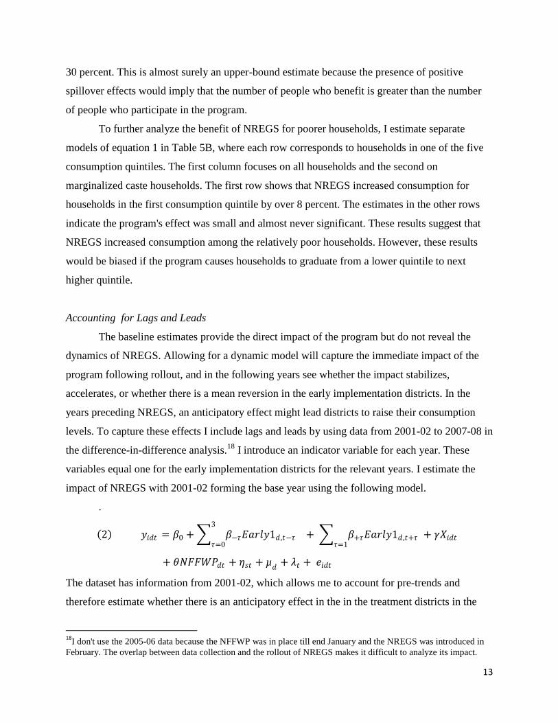
Accounting for Lags and Leads

The baseline estimates provide the direct impact of the program but do not reveal the

dynamics of NREGS. Allowing for a dynamic model will capture the immediate impact of the

program following rollout, and in the following years see whether the impact stabilizes,

accelerates, or whether there is a mean reversion in the early implementation districts. In the

years preceding NREGS, an anticipatory effect might lead districts to raise their consumption

levels. To capture these effects I include lags and leads by using data from 2001-02 to 2007-08 in

the difference-in-difference analysis.18

I introduce an indicator variable for each year. These

variables equal one for the early implementation districts for the relevant years. I estimate the

impact of NREGS with 2001-02 forming the base year using the following model.

.

2 𝑦𝑖𝑑𝑡 = 𝛽0 + 𝛽−𝜏𝐸𝑎𝑟𝑙𝑦1𝑑 ,𝑡−𝜏

3

𝜏=0+ 𝛽+𝜏𝐸𝑎𝑟𝑙𝑦1𝑑 ,𝑡+𝜏

𝜏=1 + 𝛾𝑋𝑖𝑑𝑡

+ 𝜃𝑁𝐹𝐹𝑊𝑃𝑑𝑡 + 𝜂𝑠𝑡 + µ𝑑

+ 𝜆𝑡 + 𝑒𝑖𝑑𝑡

The dataset has information from 2001-02, which allows me to account for pre-trends and

therefore estimate whether there is an anticipatory effect in the in the treatment districts in the

18

I don't use the 2005-06 data because the NFFWP was in place till end January and the NREGS was introduced in

February. The overlap between data collection and the rollout of NREGS makes it difficult to analyze its impact.

14

years leading up to the introduction of the program. The coefficient for 2007-08 gives the

estimates for the lagged effect of the program in the early implementation districts and t=2004.

𝜂𝑠𝑡 is either the state-specific linear time trend or state-by-year fixed effects. The state time trend

allows states to follow different trends while the state-by-year fixed effect captures any state

specific shock to consumption (e.g., as a result of policies that may be passed by state

governments).

Before NREGA was introduced, the government had started the National Food For Work

Program (NFFWP) in November 2004. The 150 most backward districts were to receive work in

public works in exchange for food grains and wage payment. This program was subsumed under

the Rural Employment Guarantee Program that was rolled out from 2006 and the 150 backward

districts were among the 200 early implementation districts. Although the NFFWP was

discontinued in the districts before the NREGA was introduced in February 2006, there is

concern that the effect one sees from NREGA may be partly due to the NFFWP. The survey

teams that visited some of the most backward districts of the country from May to June 2006 had

reported little activity under NREGA.19

While this is worrying, it also suggests that the districts

were not continuing the NFFWP and the impact of NREGA that I estimate using the difference-

in-difference approach is not picking up the work from the earlier Food for Work program. I

analyze NREGA in the context of the NFFWP being in place. To ensure that the National Food

For Work Program, introduced in 2004, does not influence the estimate of NREGA on household

consumption, I introduce the variable NFFPW, which equals one for the 150 districts that

received NFFWP.

Results for the analysis using data from 2001-02 to 2007-08 are presented in Table 6.

Similar to Table 4, the first two columns show the results for all households, the next two for

marginalized caste households, and the last two include the districts that received the program in

the second and third phase of the rollout in the "late implementation" group. The odd numbered

columns use the state linear time trend and the even numbered columns use the state-by-year

fixed effects. I find the introduction of NREGS increased consumption for all households by 8.7

percent. These results are significant at the 1 percent level. State-by-year fixed effects account

19

Report on Implementation of NREGA, Centre for Budget and Governance Accountability, New Delhi

15

for concurrent expansion of other public programs and its inclusion leaves the results largely

unaffected.20

To analyze the impact on households who are more likely to use and benefit from the

program, I focus on marginalized caste households since they have greater percentage Below the

Poverty Line than the "General Caste" households. I find that NREGS increases consumption by

nearly 10 percent and the use of state-by-year fixed effects does not reduce the effect.

Robustness Checks

The introduction of the NFFWP in the 150 backward districts (which coincides with the

200 early implementation) leads to a positive and significant effect in the "early" districts for

2004-05 (Figure 4). However, this effect is not large and is within 10 percentage points. The fact

that NFFWP has an impact on consumption, may lead one to think that the effect of NREGS is

partly a result of Food for Work Program. To address this concern I exclude the 150 districts that

received the NFFWP.21

The results are depicted in Figure 5, which plots the β coefficients on the

vertical axis against year which is on the horizontal axis. The coefficient for 2004-05 is near zero

while the coefficient for 2006-07 is 5 percent. The standard errors are large since the sample has

been reduced. The exclusion allows us to focus solely on districts where the increase in

consumption for the early implementation districts cannot be credited to the NFFWP. Therefore,

the NREGS does lead to an increase in consumption and that increase cannot be completely

attributed to having had the NFFWP since 2004. Figure 5 also shows that for the years preceding

the program, the coefficient is near zero, indicating that there is no anticipatory effect of NREGS

in these districts.

The effect of NREGS instead of increasing or flattening out in 2007-08, decreases by 1.3

percentage points (Figure 4). This can be explained by the overlap in the survey period which

continued till end June 2008 (Figure 2) and the introduction of NREGS in April 2008 in the

control districts. The overlap corresponds to the lean agricultural season and households in the

control group were likely to work under NREGS. This may cause a downward bias to the effect

20

Including the group of districts that implemented the program in “phase 2" in the late implementation (control)

group reduces the point estimate to around 7 percent in 2006-07 and this is significant. 21

The regression does not include district fixed effects. Instead I use an indicator variable for early implementation

districts. I also trim the sample and reduce the number of late implementation districts by excluding the ones which

are least backward (i.e., have a rank greater than 350).

16

of the program. To account for the overlap, I omit the months from April to June in 2008.22

The

estimates in Figure 6 show that the dip flattens out when I exclude the overlapping period

implying that the effect of NREGS remains relatively stable in the latter years.

In Table 7, I conduct a similar difference-in-difference analysis and use districts that

received NREGS in Phase 2 as my early implementation group while maintaining the same

control group. The focus is now on the coefficient for 2007-08 since the Phase 2districts

received the program in April 2007 but the control districts had yet to receive the program.

NREGS was introduced in the control districts in April 2008. I find no effect on consumption

while Azam (2012) finds a significant impact on public sector employment for 2007-08 for

districts that received the program in Phase 2. By looking at the consumption data it would seem

that the impact does not translate to increases in household consumption. The overlap in the

survey period and rollout of NREGS in the control districts, which coincides with the lean

agricultural season, may have also played a role in seeing no effect of the program for Phase 2

districts.

Seasonal Variation and Consumption Smoothing

The NREGS was specifically designed to provide a fallback source of employment when

work from agriculture is scarce or inadequate. If the effect of NREGS is similar during the lean

and non-lean agricultural season then households use the income earned from the program to

smooth consumption over the two seasons. I use a difference-in-difference-in-difference model

(DDD) to analyze whether households in the "early" districts smooth consumption over the lean

and non-lean season. Figure 1 shows that households use the program primarily during the lean

season (January to June)). Households also know that the program is not temporary and they

have access to it every year. Given these facts, it is necessary to analyze whether households

smooth consumption or whether consumption is contemporaneously correlated with income.

Poor households, due to liquidity constraints, may not be in a position to save during the lean

season to smooth consumption over the entire year. Time preference may also play a role,

whereby household's present discount value of future consumption can lead them to have higher

levels of consumption during the lean agricultural season by working under NREGS.

22

NSSO collects data in four sub-rounds . In each sub-round an equal number of First Stage Units are surveyed to

ensure uniform spread of the sample over the entire survey period.

17

First, I analyze whether NREGS separately increases consumption in the non-lean

season and the lean season. The "late" districts continue to forms my control group since they do

not have access to the program to smooth consumption. I assume that the "late" districts continue

with the same pattern of seasonal consumption in the absence of public programs. Table 8A

shows the results of an equation similar to equation (2) where the first column focuses on lean

season observations and the second column on non-lean season observations.23

The results

indicate no pre-trends implying that the early and late implementation districts had a similar

pattern before the NFFWP or NREGS was introduced. NREGS increased consumption by

around 7 percent in the non-lean season (July to December of 2006) and by nearly 10 percent in

the lean season (January to June of 2007) . This suggests households used the program to

increase consumption level in both the lean and non-lean season. The increase in the non-lean

season (which is before the lean season) can be explained by households working under NREGS

in the agricultural season or by household increasing consumption in anticipation of higher

income by working under NREGS during the lean season. For 2007-08, the increase is around 9

percent in the non-lean season. This may be a combination of anticipatory effect and households

saving part of the increase in income in 2006-07 to increase future consumption.

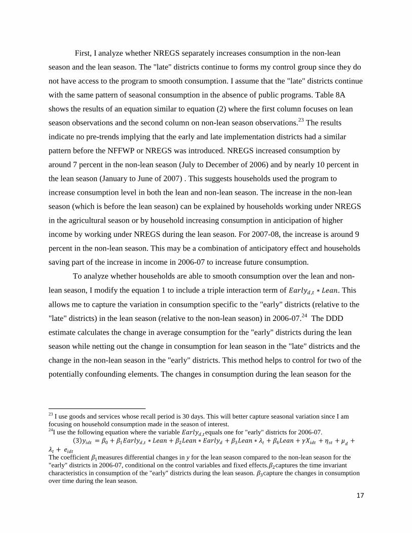
To analyze whether households are able to smooth consumption over the lean and non-

lean season, I modify the equation 1 to include a triple interaction term of 𝐸𝑎𝑟𝑙𝑦𝑑 ,𝑡 ∗ 𝐿𝑒𝑎𝑛. This

allows me to capture the variation in consumption specific to the "early" districts (relative to the

"late" districts) in the lean season (relative to the non-lean season) in 2006-07.24

The DDD

estimate calculates the change in average consumption for the "early" districts during the lean

season while netting out the change in consumption for lean season in the "late" districts and the

change in the non-lean season in the "early" districts. This method helps to control for two of the

potentially confounding elements. The changes in consumption during the lean season for the

23

I use goods and services whose recall period is 30 days. This will better capture seasonal variation since I am

focusing on household consumption made in the season of interest. 24

I use the following equation where the variable 𝐸𝑎𝑟𝑙𝑦𝑑 ,𝑡equals one for "early" districts for 2006-07.

3 𝑦𝑖𝑑𝑡 = 𝛽0 + 𝛽1𝐸𝑎𝑟𝑙𝑦𝑑 ,𝑡 ∗ 𝐿𝑒𝑎𝑛 + 𝛽2𝐿𝑒𝑎𝑛 ∗ 𝐸𝑎𝑟𝑙𝑦𝑑 + 𝛽3𝐿𝑒𝑎𝑛 ∗ 𝜆𝑡 + 𝛽4𝐿𝑒𝑎𝑛 + 𝛾𝑋𝑖𝑑𝑡 + 𝜂𝑠𝑡 + µ𝑑

+

𝜆𝑡 + 𝑒𝑖𝑑𝑡

The coefficient 𝛽1measures differential changes in y for the lean season compared to the non-lean season for the

"early" districts in 2006-07, conditional on the control variables and fixed effects.𝛽2captures the time invariant

characteristics in consumption of the "early" districts during the lean season. 𝛽3capture the changes in consumption

over time during the lean season.

18

treatment districts is not a result of changes in consumption in the lean season for all districts,

nor is it a result of changes in consumption for all households in "early" districts.

Table 8B, Panel A, shows that households had a similar level of per capita consumption

in the lean and non-lean season before the program was implemented. Panel B, column 1, reports

the results for the equation which uses data from 2001-02 and 2003. Here 𝐸𝑎𝑟𝑙𝑦𝑑 ,𝑡 ∗ 𝐿𝑒𝑎𝑛 equals

one for the lean season observation for year 2001 (with base year 2003) and the early

implementation districts. The point estimate of 𝛽1 small and statistically insignificant indicating

that households were smoothing consumption over the lean and non-lean seasons in the pre-

program period.

With the introduction of NREGS, consumption in lean season increased by over 3

percent, but this is statistically insignificant. This suggests that credit constraints or uncertainty

about the benefits from NREGS did not cause households to have significantly different levels of

consumption in the lean and non-lean seasons. Thus households were able to anticipate the

benefit from the program and accordingly adjust their spending decisions to try to smooth

consumption.

Results for Household Spending by Consumption Categories

In Tables 9 through 11, I shift the focus from overall consumption expenditure to

household spending decisions on the various consumption categories. Each column provides

estimates from separate regressions using equation (2) with state linear time trend specification.

The top panel focuses on all households while the lower panel concentrates on marginalized

caste households.

Apart from increasing consumption, the program may have led households to change the

way they allocate income among the different categories. Table 9 presents the results for

essential food items. The program does not have an economic or statistically significant effect on

cereals or 'cereal substitutes' (like tapioca) which are cheaply available high starch items and

have very low nutritional content. The impact on pulses is not significantly different from zero.25

Households instead used the program to increase consumption of protein by around 12 percent

to incorporate more nutrition and higher caloric items in their diet. Marginalized caste

25

For 2004-05 there is almost a 14 percent increase in pulse consumption. This may be a result of the National Food

for Work Program being used in the 150 backward districts (which was later subsumed in the "early" districts under

NREGS).

19

households followed the same pattern and raised protein consumption by nearly 14 percent. Milk

consumption also increased by nearly 13 percent. It would seem that in terms of the major food

items, households raised consumption of items that have a higher nutritional value. There has

been a trend of increasing calorie from fat (Deaton and Dreze (2009). In keeping with this trend,

consumption of oil and other cooking fats increased by 7 percent. The program also increased

fuel and light consumption by 7.7 percent.

Since women are responsible for majority of the housework and child care, work that

takes them far from the house is not feasible. The Act makes it easier for women to participate

under NREGS by ensuring that workers are provided work within 5 kilometers of their home.

The minimum wage guarantee under NREGS has attracted women because women typically

receive less wages than men in casual works. As a result women constitute more than half of the

workforce under NREGS. The formal payment for work also allows women to know their

contribution to the total household budget. This may increase their bargaining power in

household decision making as seen in Qian (2005) and Jensen and Miller (2010). In the

literature, increase in women’s income is associated with increases in household well-being,

especially for children..

Table 10 focuses on household medical and educational expenditure, and expenditure on

intoxicants, beverages and tobacco. For institutional medical expenditures, the effect of NREGS

is not significantly different from zero. This is not surprising since the program pays minimum

wage and is unlikely to affect spending on big expenditure items.26

The program has a small

positive effect on educational spending but this is not statistically significant. The NREGS may

have improved the working of the Mid Day Meal Program, which provides school children with

food during the middle of the school day, and lowered overall education costs.27

Also, poorer

26

Institutional medical expenditures refer to goods and services received as an in-patient in private as well as

Government medical institutions like nursing homes, and hospitals. These goods and services include payments for

medicine, doctor's and surgeon's fee, medical tests and X-rays, and hospital and nursing charges. 27

I also conduct an ordered logit on education categories (not-literate, literate but without formal education, literate

but below primary, primary, middle, secondary, and higher secondary and above) to analyze if the program has an

effect on the number of years people attend school. I restrict the sample to individuals with who are between the age

of 5 and 18 and use data from 2003 and 2006-07. I include an interaction term 𝐸𝑎𝑟𝑙𝑦𝑑 ,𝑡 which equals one for

individuals in "early" districts and the year is 2006-07. I also include the same individual and household level

characteristics as in equation (1). District and time fixed effects are used along with state time trends. I find the

program has no significant impact in increasing the log odds of moving to a higher education category. I also use a

smaller number or categories (primary and less, middle, and high school and above) and find no significant impact

of the program.

20

households who have a lower expected return from education in rural areas may view the

program as an opportunity to enter the labor force at an earlier age.

The program increased consumption of beverages (example tea, coffee, bottled drinks,

refreshments) which falls under the luxury consumption item category. Overall, the expenditure

on intoxicants and tobacco did not increase significantly in 2006-07. In order to analyze whether

the presence of children affect consumption patterns, I run separate regression on households

with children and households without children. The results are in Table 11. For households

without children, NREGS increases alcohol consumption by around 30 percent. For households

with children the effect is negative but insignificant. The opposite pattern is seen for milk

consumption. For households with children, NREGS significantly increases milk consumption

by nearly 15 percent while there is no effect for households without children. In terms of health,

spending on non-institutional medical items is positive and significant for households with

children and there is no effect on households without children. Therefore, increase in women's

contribution to household income by participating in NREGS impacts household wellbeing only

when there are children present in the household.

Expenditure on household durable goods are discussed in Table 12. NREGS has a

positive effect on spending on furniture. This may be a result of the increase in income from the

program or an increase in access to credit by working in a program that guarantees employment

for 100 days of the year. The increase in disposable income also increased spending on bedding

which, unlike furniture, has limited resale value. There is no effect on clothing and footwear.

This pattern is true for marginalized caste households and the population in general.

Indian households purchase jewelry, especially gold, as an instrument for savings. In

rural India, where financial instruments for saving are limited, households buy gold since it is a

liquid asset which can be sold easily for cash in times of need. Nearly 70 percent of the gold sold

in India is purchased in rural India in the form of jewelry (Reserve Bank of India, 2013).

Therefore, if the program increases household income and thereby the ability to save, it will be

reflected through increased purchase of jewelry. However, the effect of NREGS for jewelry

consumption is positive but not significant. This may be because the program increases income

for poor households but it is not sufficient to lead to savings for the poor households who work

in NREGS.

21

5. Conclusion

In the last decade low-income countries have predominantly used public works programs

to address issues of poverty and seasonal unemployment. By studying NREGS, I analyze a

program whose objectives reflect worldwide commitment to reducing poverty to achieve the

Millennium Development Goals. Although there have been concerns about the effectiveness of

the program, the paper provides evidence that an anti-poverty workfare programs that is designed

like the NREGS leads to an overall increase in consumption and this holds true for households

who belong to the lowest consumption quintile. The impact on the marginalized caste group,

who constitute the relatively poorest section of the population, is positive and significant,

indicating that discrimination and other barriers to entry did not prevent them from improving

household wellbeing. The increase in consumption occurs both over the lean and non-lean

agricultural seasons and rural households are able to anticipate the permanent increase in overall

income and accordingly smooth consumption.

In this paper my purpose has been to estimate the intent-to-treat effect of the program and

assess the overall effect of NREGS on household consumption for the treated districts. I have not

specifically assessed the cost to the private sector from potential crowding out (of labor at below

minimum wages) due to NREGS. The paper also focuses on the rural area and the cost to urban

businesses brought about by changes in seasonal rural-urban migration as a result of higher

expected wage in the rural sector has not been examined. To analyze these above questions it is

crucial to understand the exact mechanism through which NREGS affects the various sections of

the population.

Further work that focuses on the indirect benefits of the Rural Employment Guarantee

program would be of great value. The program can have indirect benefits for the rural poor

which impact household wellbeing. For instance, the majority of the public works under the

program focus on water projects other than irrigation. Logically such works would increase

water supply in villages and reduce the amount of time women devote to collecting water for

household purposes which in turn may improve women's labor productivity. Access to clean

water can also have a positive effect on health outcomes which can positively impact labor

productivity. Therefore, apart from analyzing the overall benefits of the program in terms of

household consumption and employment, evaluating the indirect benefits would be useful for

policy makers and planners in India and in other developing countries with similar programs.

22

Data Appendix

The paper uses the nationally representative household data from the Consumption

Expenditure Survey conducted by the National Sample Survey Organization (NSSO) for 2001-

02, 2003, 2004-05, 2006-07 and 2007-08, to cover the years preceding and following the rollout

of the program in Phase 1 districts (which started in February 2006). The NSSO collects

information on consumption expenditure every year and covers nearly all the districts in India.

These annual cross-sectional surveys are administered using a stratified multi-stage random

sampling where the lowest identifiable geographic unit for households in the sample is the

district.

I use the 19 major states of India and restrict the sample to rural households since the

program has only been introduced in the rural areas. The States are: Andhra Pradesh, Assam,

Bihar, Chhattisgarh, Gujarat, Haryana, Himachal Pradesh, Jharkhand, Karnataka, Kerala,

Madhya Pradesh, Maharashtra, Orissa, Punjab, Rajasthan, Tamil Nadu, Uttaranchal, Uttar

Pradesh and West Bengal. They account for nearly 96% of India’s population in the 2001

Census. Jammu and Kashmir and the Northeastern states have not been included since they have

different economic and political characteristics from the other states in the country. I exclude

Delhi and the Union territories from the sample.

The 2004-05 round is part of the large sample survey that the NSSO administers every

five years. Since the Program was implemented across districts over the period 2006-2009, the

2004-05 survey is the only large sample survey used in this paper. Though the size of the

samples vary, I can combine the large and small sample surveys because the NSSO provides

weights for each household to ensure that datasets are representative of the entire population. I

use these weights to analyze the impact of the program.

NSSO uses a stratified multi-stage sampling method to collect data. Each district of a

State is stratified into a rural and urban stratum. The multi-stage sampling consists of the First

Stage Unit (FSU) and the Ultimate Stage Unit (USU). The FSUs for the rural sector are the

villages listed in the Census of 2001 and the USUs are the households in the villages. Sample

size allocated to each stratum is in proportion to the population of 2001. The villages to be

sampled are selected by probability proportional to size with replacement (PPSWR), size being

23

the population of the village. Sampling of households from the selected villages is based on

affluence and the nature of principal activity (agricultural or non-agricultural).

The main categories in the consumption expenditure survey are 'food', 'fuel and light',

'clothing and footwear', 'education and medicine' and 'durable goods'. The questionnaire used to

collect the data is comparable across the various rounds since they use the same recall period for

the different consumption categories. However, the 2004-05 round uses two recall periods (a 30-

day and 365-day recall period) in the 'clothing and footwear' and 'durable goods' categories,

whereas the other years use the 365-day reference period for the same broad categories. By

relegating the 30 day reference period and only using the 365-day reference period for the 2004-

05 round for these categories make it comparable to other years. Therefore, I am able to use the

five survey rounds for all the analyses.

In order to identify which districts received the program in each of the three phases, I

combined the NSSO data, which includes district-level identifiers, with data I obtained from the

NREGA website, which reports the year in which districts received the program.

I also include in the dataset the district level information on percentage SC/ST

population, output per agricultural worker and agricultural wages per day from the Planning

Commission Report on Identification of Districts for Wage and Self Employment Programmes

(2004).

Calculation of Consumption Expenditure by NSSO

If households purchase and consume certain goods or services, the value of consumption

is used as purchase value. For household consumption from commodities received in exchange

of goods and services, home production and free collection, the NSSO follows the following

rules to impute value. Depending on the recall period, the value of goods and services from free

collection, loans, gifts, and items received in exchange of other goods and services are imputed

at the rate of average local retail prices. Home production is imputed at the ex farm or ex factory

rate.

Treatment and Control Districts

I use the districts that received the program in Phase 1, 2006-07, as my treatment group

while the control group consists of the districts that received the Program in Phase 3, 2008-09.

24

2003 forms the base period for this analysis. The reason for using districts that received the

program in Phase 3 as the comparison group rests on the timing of the rollout of the program and

its overlap with the collection period of the NSSO data for consumption expenditure. Figure 2

shows the timeline of the above events. The top panel shows the rollout of the program and the

bottom panel shows the survey collection period. The NSSO data used to analyze the program is

collected from July 2006 to June 2007 (63rd Round) while the districts received the program in

Phase 2 from April 2007. There is an overlap of three months in collection of the data and use of

the program by districts that received the program in Phase 2. This makes these districts not a

valid comparison group. Also, the months from April to June are the lean seasons of agriculture

when household demand for work under the program is high. Therefore, the overlap would make

it difficult to assess the impact of the program if districts receiving the program in Phase 2 form

the control group. To avoid the problem of overlap I use the district which received the Program

in April 2008, i.e. in Phase 3, since the rollout for these districts is after the survey was carried

out for the 63rd Round. The timeline also shows that the cleanest data collection period on which

to focus the analysis is July 2006 to end June 2007. This is the only year where one group of

districts (all early implementation districts) had received the program while one group of districts

(all the late implementation districts) had not received the program. If the analysis focuses on the

data collected from July 2007 to end June 2008 (64th Round), there would be a problem of

overlap because the late implementation districts received the Program in April 2008.

Agricultural (Non-lean) and Lean Season

The agricultural season in India is from July to November. The NSSO collects data in 4

sub-rounds, each has a duration of three months. An equal number of First Stage Units are

sampled in these rounds to ensure uniform spread over the entire survey period. I have used the

first two sub-rounds (July to December) as the agricultural (non-lean) season. Thus I have

included December in the non-lean season when it should have been included in the lean season.

It should also be noted that the non-lean season for 2007-08 does not overlap with the rollout of

the Program in the control districts (April 2008).

25

References:

Aiyar, Yamini, and Salimah Salimah. "Transparency and Accountability in NREGA: A Case Study of

Andhra Pradesh." Working Paper, 2009.

Alaniz, Enrique, T. H. Gindling, and Katherine Terrell. "The Impact of Minimum Wages on Wages,

Work and Poverty in Nicaragua." Labour Economics 18, no. 1 (2011): S45-S59.

All India Report on Evaluation of NREGA: A survey of 20 Districts. Planning Commission of India,

2008.

Angrist, Joshua D, and Jorn-Steffen Pischk. Mostly Harmless Econometrics: An Empiricist's Companion .

Princeton University Press, 2008.

Azam, Mehtabul. "The Impact of Indian Job Guarantee Scheme on Labor Market Outcomes:Evidence

from a Natural Experiment." IZA Discussion Paper No. 6548, 2012.

Azam, Mehtabul, Céline Ferré, and Mohamed Ajwad. "Did Latvia's public works program mitigate the

impact of the 2008-2010 crisis?" World Bank Policy Research Working Paper, no. 6144 (2012).

Banerjee, Abhijit, Marianne Bertrand, Saugato Datta, and Sendhil Mullainathan. "Labor market

discrimination in Delhi: Evidence from a field experiment." Journal of Comparative Economics 37, no. 1

(2009): 14-27.

Berg, Erlend, Sambit Bhattacharyya, Rajasekhar Durgam, and Manjula Ramachandra. " Can Rural Public

Works Affect Agricultural Wages? Evidence from India." Unpublished, 2012.

Besley, Timothy, and Stephen Coate. "Workfare Versus Welfare: Incentive Arguments for Work

Requirements in Poverty-Alleviation Programs." The American Economic Review 82, no. 1 (1992): 249-

261.

Blundell, Richard, Monica Costa D, Meghir Costas, and Jonathan Shaw. " The Long-Term Effects of In-

Work Benefits in a Life-Cycle Model for Policy Evaluation." CeMMAP working papers CWP07/11,

2011.

Chaudhuri, Shubham, Gaurav Datt, and Martin Ravallion. "Does Maharashtra's Employment Guarantee

Scheme Guarantee Employment? Effects of the 1988 Wage Increase." Economic Development and

Cultural Change 41, no. 2 (1993): 251-275.

Deaton, Angus. "Looking for Boy-Girl Discrimination in Household Expenditure Data." The World Bank

Economic Review 3, no. 1 (1989): 1-15.

Deaton, Angus. "Savings in Developing Countries: Theory and Review." In Proceedings of the World

Bank Annual Conference on Development Economics 1989., pp. 61-108. World Bank, 1990.

Deaton, Angus, and Jean Dreze. "Food and Nutrition in India: Facts and Interpretations ." Economic and

Political Weekly, 2009.

26

Del Ninno, Carlo, Kalanidhi Subbarao, and Annamaria Milazzo. "How to Make Public Works Work: A

Review of the Experiences." World Bank, Human Development Network, 2009.

Delay in Payment of Wages to NREGA Workers. Circular, Government of India, 2009.

Doss, Cheryl. "The Effects of Intrahousehold Property Ownership on Expenditure Patterns in Ghana."

Journal of African Economies 15, no. 1 (2006): 149-180.

Dreze, Jean, Reetika Khera, and Siddhartha. "Corruption in NREGA: Myth and Reality." The Hindu.

January 22, 2008.

Duflo, Esther, and Christopher Udry. "Intrahousehold Resource Allocation in Cote d'Ivoire: Social

Norms, Separate Accounts and Consumption Choices." National Bureau of Economic Research w10498.

(2004).

Dutta, Puja, Rinku Murgai, Martin Ravallion, and Dominique Van de Walle. "Does India's Employment

Guarantee Scheme Guarantee Employment?" World Bank Policy Research Working Paper 6003, 2012.

Gilligan, Daniel O., John Hoddinott, and Alemayehu Seyoum Taffesse. "The impact of Ethiopia's

Productive Safety Net Programme and its linkages." The Journal of Development Studies 45, no. 10

(2009): 1684-1706.

GOI, Government of India. Employment and Unemployment Situation in India, 2004-05. National

Sample Survey Organisation , 2006.

GOI, Government of India. "Informal Sector and Conditions of Employment in India 2004-05." National

Sample Survey Organisation , Ministry of Statistics & Programme Implementation , 2007.

GOI, Government of India. "Mahatma Gandhi National Rural Employment Guarantee Act - Report to the

People." Department of Rural Development, Ministry of Rural Development, New Delhi, 2013.

GOI, Government of India. "Report of the Expert Group to Review the Methodology for the Estimation

of Poverty." Planning Commission, 2009.

Government of India, Ministry of Rural Development. The Mahatma Gandhi National Rural Employment

Guarantee Act 2005. http://nrega.nic.in/netnrega/home.aspx (accessed September 23, 2013).

Haddad, Lawrence, Johnt Hoddinot, and Harold Alderman. "Intrahousehold Resource Allocation: An

Overview." (The World Bank) 1255 (1994).

Hahn, Jinyong, Petra Todd, and Wilbert Van der Klaauw. "Identification and Estimation of Treatment

Effects with a Regression-Discontinuity Design." Econometrica 69, no. 1 (2001): 201-209.

Heckman, J., LaLonde, R., and R. Smith. The Economics and Econometrics of Active Labor Market

Programs. Vol. 3, in Handbook of Labor Economics, edited by O. Ashenfelter and D. Card, 1865-2097.

1999.

Hoddinott, John, and Lawrence Haddad. "Does Female Income Share Influence Household Expenditures?

Evidence from Côte d'Ivoire." Oxford Bulletin of Economics and Statistics, 1995: 77-96.

27

Hoynes, Hilary Williamson, and Diane Whitmore Schanzenbach. "Work Incentives and the Food Stamp

Program." Journal of Public Economics 96, no. 1 (2012): 151-162.

Imbens, Guido W., and Thomas Lemieux. "Regression Discontinuity Designs: A Guide to Practice."

Journal of Econometrics 142, no. 2 (2008): 615-635.

Jacob, Naomi." ,. "The Impact of NREGA on Rural-Urban Migration: Field survey of Villupuram

District, Tamil Nadu." 2008. http://www.ccs.in/ccsindia/downloads/intern-papers-08/NREGA-Paper-

202.pdf (accessed 10 10, 2013).

Jadhav, Vishal. "Elite Politics and Maharashtra's Employment Guarantee Scheme." Economic and

Political Weekly , 2006: 5157-5162.

Jalan, Jyotsna, and Martin Ravallion. "Estimating the Benefit Incidence of an Antipoverty Program by

Propensity-Score Matching." Journal of Business & Economic Statistics 21, no. 1 (2003): 19-30.

Kumar, Sunil Mitra. "Does Access to Formal Agricultural Credit Depend on Caste?" World

Development, 2012.

Lee, David S., and Thomas Lemieux. "Regression Discontinuity Designs in Economics." The Journal of

Economic Literature 48, no. 2 (2010): 281-355.

Lemos, Sara. "Minimum Wage Effects in a Developing Country." Labour Economics 16, no. 2 (2009):

224-237.

Luke, Nancy, and Kaivan Munshi. "Social affiliation and the demand for health services: Caste and child

health in South India." Journal of Development Economics 83, no. 2 (2007): 256-279.

Moore, Mick, and Vishal Jadhav. "The politics and bureaucratics of rural public works: Maharashtra's

employment guaranteed scheme." Journal of Development Studies 42, no. 8 (2006).

Morduch, Jonathan. "Income Smoothing and Consumption Smoothing." The journal of economic

perspectives 9, no. 3 (1995): 103-114.

Munshi, Kaivan, and Mark R. Rosenzweig. "Traditional Institutions Meet the Modern World: Caste,

Gender and Schooling Choice in a Globalizing Economy." American Economic Review 96, no. 4 (2006):

1225-1252.

National Food For Work Programme Guidelines. Department of Rural Development, Ministry of Rural

Development, New Delhi: Government of India.

National Rural Employment Guarantee Act 2005 (NREGA), Report of the Second Year, April 2006 –

March 2007. Department of Rural Development, Ministry of Rural Development, New Delhi:

Government of India.

Qian, Nancy. "Missing Women and the Price of Tea in China: The Effect of Sex-Specific Earnings on

Sex Imbalance." The Quarterly Journal of Economics 123, no. 3 (2008): 1251-1285.

28

Ravallion, Martin. Evaluating Anti-Poverty Programs. Vol. 4, in Handbook of Development Economics,

edited by T. P. Schultz and John Strauss, 3787-3846. Amsterdam, 2007.

Report of the Task Force: Identification of Districts for Wage and Self Employment Programmes.

Planning Commission of India, 2003.

Report of the Working Group to Study the Issues Related to Gold Imports and Gold Loans by NBFCs.

Reserve Bank of India, 2013.

"Report on Implementation of NREGA in Andhra Pradesh, Chattisgarh, Jharkhand and Madhya Pradesh

in May and June 2006." Centre for Budget and Governance Accountability, New Delhi , 2006.

Rosenzweig, Mark R., and Oded Stark. "Consumption Smoothing, Migration, and Marriage: Evidence

from Rural India." The Journal of Political Economy 97, no. 4 (1989): 905-926.

Rosenzweig, Mark R., and Kenneth I. Wolpin. "Credit Market Constraints, Consumption Smoothing, and

the Accumulation of Durable Production Assets in Low-income Countries: Investments in Bullocks in

India." Journal of Political Economy 101, no. 2 (1993): 223-244.

Schultz, Paul T. "Women's roles in the agricultural household: Bargaining and human capital

investments." Handbook of Agricultural Economics 1 (2001): 383-456.

Tendulkar Committee. "Report of the Expert Group to Review the Methodology for Estimation of

Poverty." Planning Commission of India, 2009.

UNDP. "Empowering Lives Through Mahatma Gandhi NREGA." 2011.

"Workers to Protest Against Corruption in NREGA." Times of India. Jaipur, March 22, 2012.

Zimmermann, Laura. "Labor Market Impacts of a Large-Scale Public Works Program: Evidence from the

Indian Employment Guarantee Scheme." Working Paper, 2012.

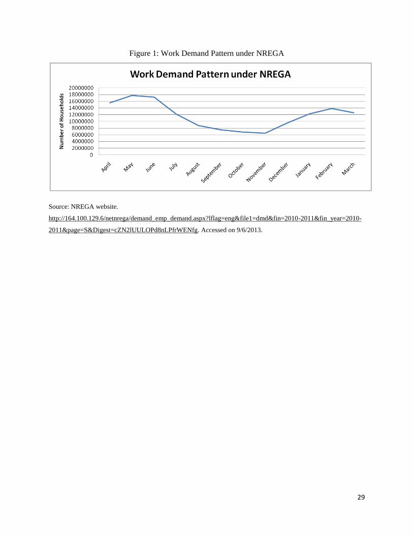
29

Figure 1: Work Demand Pattern under NREGA

Source: NREGA website.

http://164.100.129.6/netnrega/demand_emp_demand.aspx?lflag=eng&file1=dmd&fin=2010-2011&fin_year=2010-

2011&page=S&Digest=cZN2lUULOPd8nLPfrWENfg. Accessed on 9/6/2013.

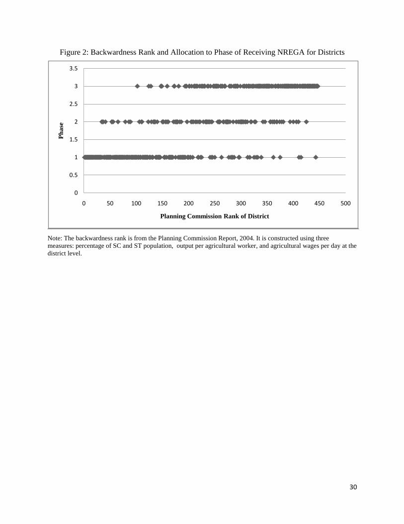
30

Figure 2: Backwardness Rank and Allocation to Phase of Receiving NREGA for Districts

Note: The backwardness rank is from the Planning Commission Report, 2004. It is constructed using three

measures: percentage of SC and ST population, output per agricultural worker, and agricultural wages per day at the

district level.

0

0.5

1

1.5

2

2.5

3

3.5

0 50 100 150 200 250 300 350 400 450 500

Ph

ase

Planning Commission Rank of District

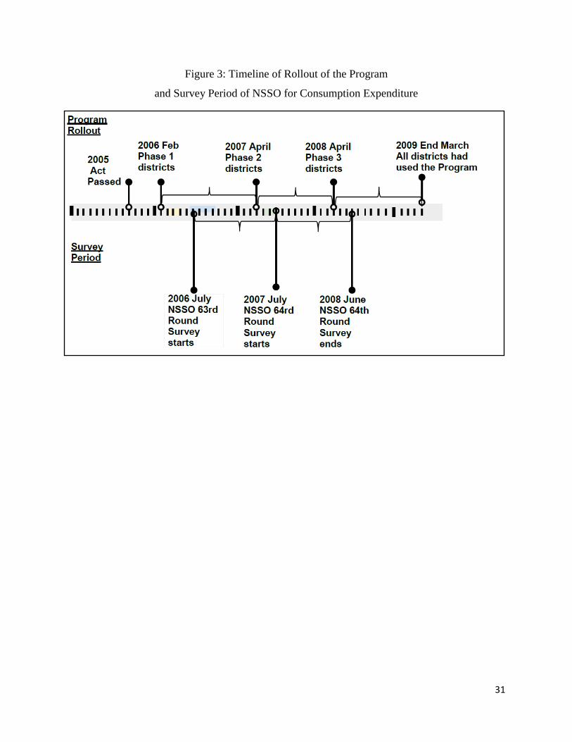
31

Figure 3: Timeline of Rollout of the Program

and Survey Period of NSSO for Consumption Expenditure

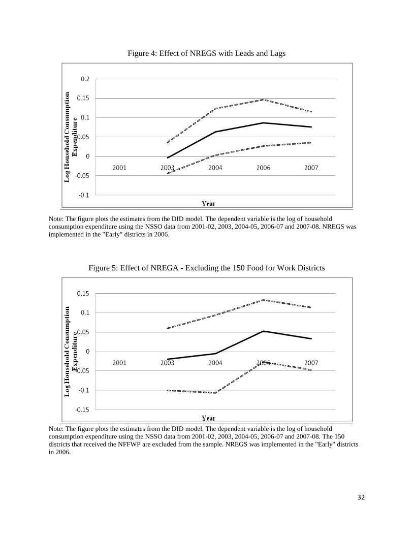
32

Figure 4: Effect of NREGS with Leads and Lags

Note: The figure plots the estimates from the DID model. The dependent variable is the log of household

consumption expenditure using the NSSO data from 2001-02, 2003, 2004-05, 2006-07 and 2007-08. NREGS was

implemented in the "Early" districts in 2006.

Figure 5: Effect of NREGA - Excluding the 150 Food for Work Districts

Note: The figure plots the estimates from the DID model. The dependent variable is the log of household

consumption expenditure using the NSSO data from 2001-02, 2003, 2004-05, 2006-07 and 2007-08. The 150

districts that received the NFFWP are excluded from the sample. NREGS was implemented in the "Early" districts

in 2006.

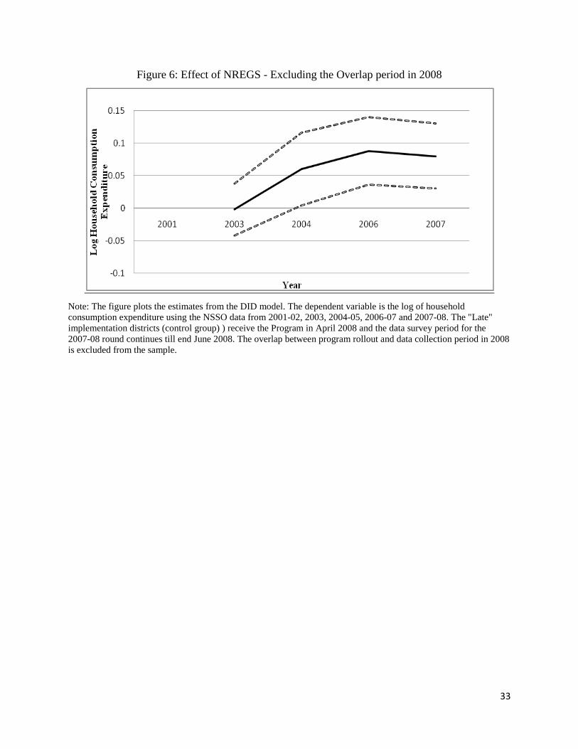
33

Figure 6: Effect of NREGS - Excluding the Overlap period in 2008

Note: The figure plots the estimates from the DID model. The dependent variable is the log of household

consumption expenditure using the NSSO data from 2001-02, 2003, 2004-05, 2006-07 and 2007-08. The "Late"

implementation districts (control group) ) receive the Program in April 2008 and the data survey period for the

2007-08 round continues till end June 2008. The overlap between program rollout and data collection period in 2008

is excluded from the sample.

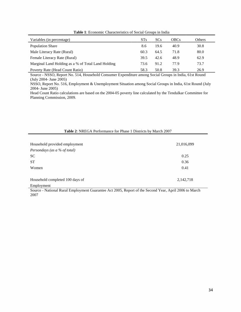
34

Table 1: Economic Characteristics of Social Groups in India

Variables (in percentage) STs SCs OBCs Others

Population Share

8.6 19.6 40.9 30.8

Male Literacy Rate (Rural)

60.3 64.5 71.8 80.0

Female Literacy Rate (Rural)

39.5 42.6 48.9 62.9

Marginal Land Holding as a % of Total Land Holding 73.6 91.2 77.9 73.7

Poverty Rate (Head Count Ratio) 58.3 50.8 39.3 26.9

Source - NSSO, Report No. 514, Household Consumer Expenditure among Social Groups in India, 61st Round

(July 2004- June 2005)

NSSO, Report No. 516, Employment & Unemployment Situation among Social Groups in India, 61st Round (July

2004- June 2005)

Head Count Ratio calculations are based on the 2004-05 poverty line calculated by the Tendulkar Committee for

Planning Commission, 2009.

Table 2: NREGA Performance for Phase 1 Districts by March 2007

Household provided employment 21,016,099

Persondays (as a % of total)

SC 0.25

ST 0.36

Women 0.41

Household completed 100 days of 2,142,718

Employment

Source - National Rural Employment Guarantee Act 2005, Report of the Second Year, April 2006 to March

2007

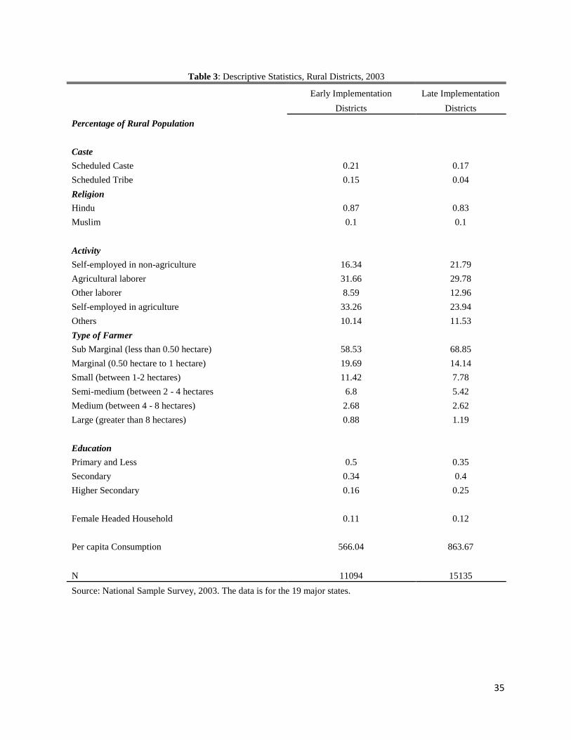
35

Table 3: Descriptive Statistics, Rural Districts, 2003

Early Implementation Late Implementation

Districts Districts

Percentage of Rural Population

Caste

Scheduled Caste 0.21 0.17

Scheduled Tribe 0.15 0.04

Religion

Hindu 0.87 0.83

Muslim 0.1 0.1

Activity

Self-employed in non-agriculture 16.34 21.79

Agricultural laborer 31.66 29.78

Other laborer 8.59 12.96

Self-employed in agriculture 33.26 23.94

Others 10.14 11.53

Type of Farmer

Sub Marginal (less than 0.50 hectare) 58.53 68.85

Marginal (0.50 hectare to 1 hectare) 19.69 14.14

Small (between 1-2 hectares) 11.42 7.78

Semi-medium (between 2 - 4 hectares 6.8 5.42

Medium (between 4 - 8 hectares) 2.68 2.62

Large (greater than 8 hectares) 0.88 1.19

Education

Primary and Less 0.5 0.35

Secondary 0.34 0.4

Higher Secondary 0.16 0.25

Female Headed Household 0.11 0.12

Per capita Consumption 566.04 863.67

N 11094 15135

Source: National Sample Survey, 2003. The data is for the 19 major states.

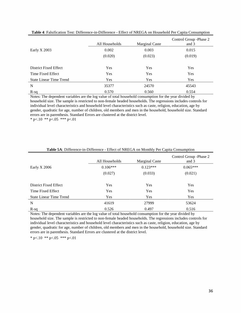
36

Table 4: Falsification Test: Difference-in-Difference - Effect of NREGA on Household Per Capita Consumption

All Households Marginal Caste

Control Group -Phase 2

and 3

Early X 2003 0.002 0.003 0.015

(0.020) (0.023) (0.019)

District Fixed Effect Yes Yes Yes

Time Fixed Effect Yes Yes Yes

State Linear Time Trend Yes Yes Yes

N 35377 24570 45543

R-sq 0.570 0.560 0.554

Notes: The dependent variables are the log value of total household consumption for the year divided by

household size. The sample is restricted to non-female headed households. The regressions includes controls for

individual level characteristics and household level characteristics such as caste, religion, education, age by

gender, quadratic for age, number of children, old members and men in the household, household size. Standard

errors are in parenthesis. Standard Errors are clustered at the district level.

* p<.10 ** p<.05 *** p<.01

Table 5A: Difference-in-Difference - Effect of NREGA on Monthly Per Capita Consumption

All Households Marginal Caste

Control Group -Phase 2

and 3

Early X 2006 0.106*** 0.123*** 0.065***

(0.027) (0.033) (0.021)

District Fixed Effect Yes Yes Yes

Time Fixed Effect Yes Yes Yes

State Linear Time Trend Yes Yes Yes

N 41619 27999 53624

R-sq 0.526 0.497 0.516

Notes: The dependent variables are the log value of total household consumption for the year divided by

household size. The sample is restricted to non-female headed households. The regressions includes controls for

individual level characteristics and household level characteristics such as caste, religion, education, age by

gender, quadratic for age, number of children, old members and men in the household, household size. Standard

errors are in parenthesis. Standard Errors are clustered at the district level.

* p<.10 ** p<.05 *** p<.01

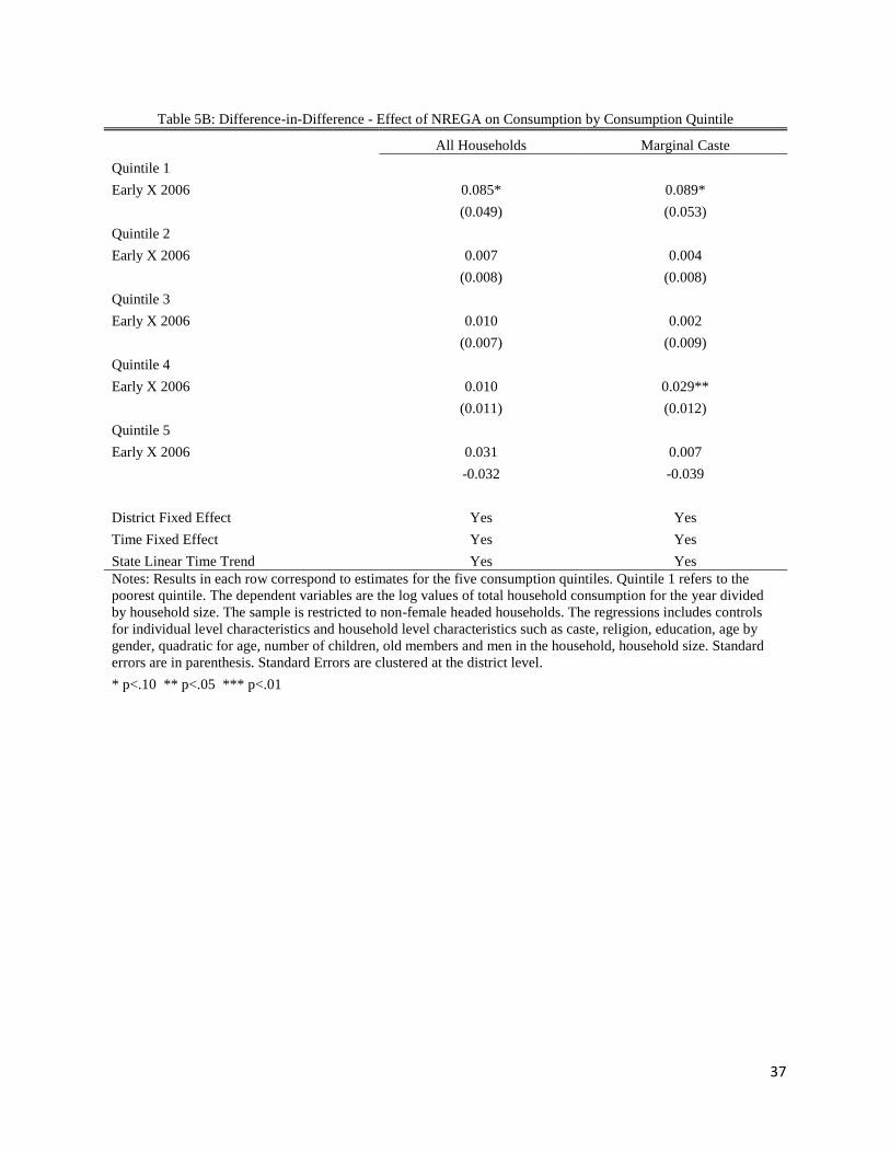
37

Table 5B: Difference-in-Difference - Effect of NREGA on Consumption by Consumption Quintile

All Households Marginal Caste

Quintile 1

Early X 2006 0.085* 0.089*

(0.049) (0.053)

Quintile 2

Early X 2006 0.007 0.004

(0.008) (0.008)

Quintile 3

Early X 2006 0.010 0.002

(0.007) (0.009)

Quintile 4

Early X 2006 0.010 0.029**

(0.011) (0.012)

Quintile 5

Early X 2006 0.031 0.007

-0.032 -0.039

District Fixed Effect Yes Yes

Time Fixed Effect Yes Yes

State Linear Time Trend Yes Yes

Notes: Results in each row correspond to estimates for the five consumption quintiles. Quintile 1 refers to the

poorest quintile. The dependent variables are the log values of total household consumption for the year divided

by household size. The sample is restricted to non-female headed households. The regressions includes controls

for individual level characteristics and household level characteristics such as caste, religion, education, age by

gender, quadratic for age, number of children, old members and men in the household, household size. Standard

errors are in parenthesis. Standard Errors are clustered at the district level.

* p<.10 ** p<.05 *** p<.01

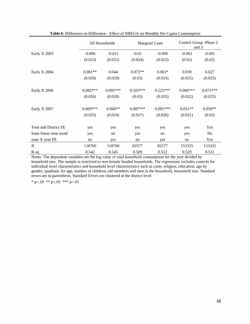
38

Table 6: Difference-in-Difference - Effect of NREGA on Monthly Per Capita Consumption

All Households Marginal Caste Control Group -Phase 2

and 3

Early X 2003 -0.006 -0.015 -0.01 -0.006 -0.002 -0.001

(0.023) (0.022) (0.024) (0.023) (0.02) (0.02)

Early X 2004 0.061** 0.044 0.072** 0.063* 0.039 0.027

(0.028) (0.029) (0.03) (0.033) (0.025) (0.025)

Early X 2006 0.082*** 0.095*** 0.103*** 0.125*** 0.066*** 0.071***

(0.026) (0.028) (0.03) (0.035) (0.022) (0.023)

Early X 2007 0.069*** 0.060** 0.087*** 0.081*** 0.051** 0.050**

(0.025) (0.024) (0.027) (0.026) (0.021) (0.02)

Year and District FE yes yes yes yes yes Yes

State linear time trend yes no yes no yes No

state X year FE no yes no yes no Yes

N 118760 118760 82577 82577 153325 153325

R-sq 0.542 0.545 0.509 0.512 0.529 0.531

Notes: The dependent variables are the log value of total household consumption for the year divided by

household size. The sample is restricted to non-female headed households. The regressions includes controls for

individual level characteristics and household level characteristics such as caste, religion, education, age by

gender, quadratic for age, number of children, old members and men in the household, household size. Standard

errors are in parenthesis. Standard Errors are clustered at the district level.

* p<.10 ** p<.05 *** p<.01

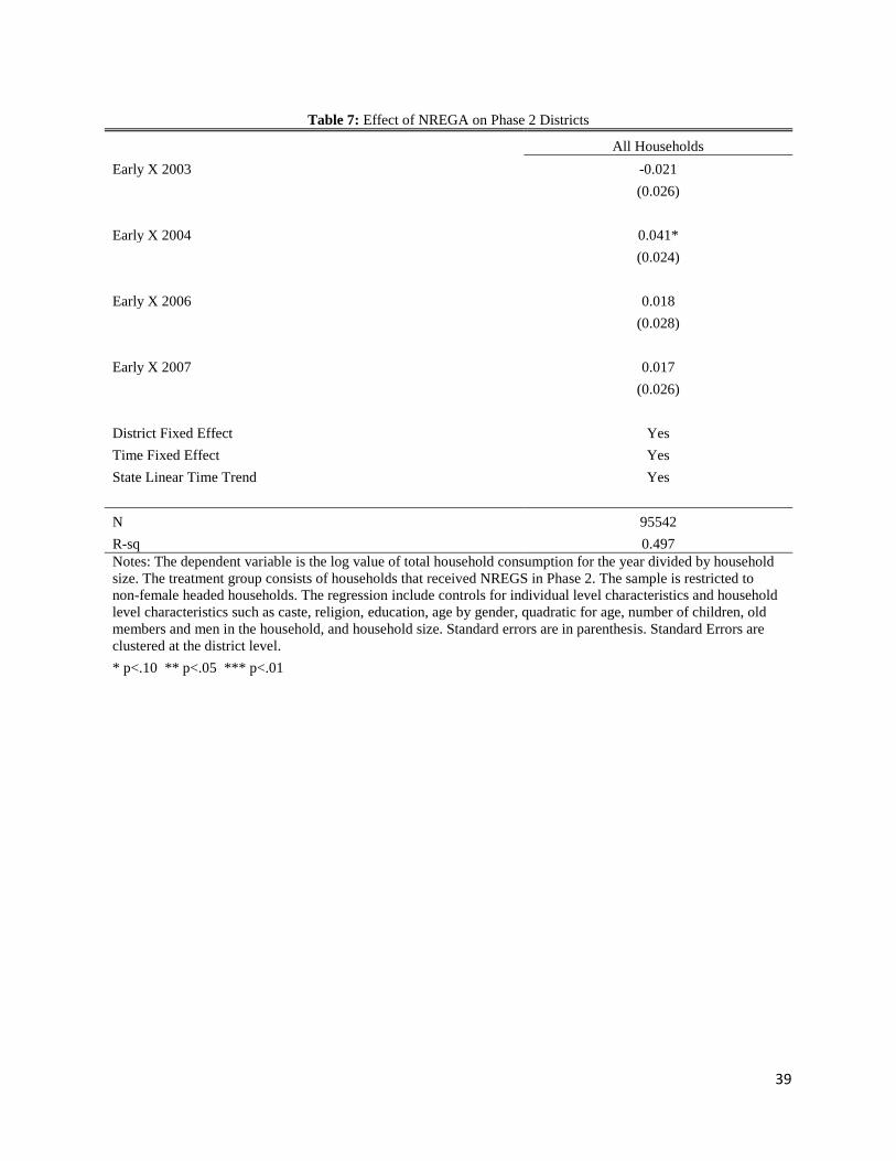
39

Table 7: Effect of NREGA on Phase 2 Districts

All Households

Early X 2003 -0.021

(0.026)

Early X 2004 0.041*

(0.024)

Early X 2006 0.018

(0.028)

Early X 2007 0.017

(0.026)

District Fixed Effect Yes

Time Fixed Effect Yes

State Linear Time Trend Yes

N 95542

R-sq 0.497

Notes: The dependent variable is the log value of total household consumption for the year divided by household

size. The treatment group consists of households that received NREGS in Phase 2. The sample is restricted to

non-female headed households. The regression include controls for individual level characteristics and household

level characteristics such as caste, religion, education, age by gender, quadratic for age, number of children, old

members and men in the household, and household size. Standard errors are in parenthesis. Standard Errors are

clustered at the district level.

* p<.10 ** p<.05 *** p<.01

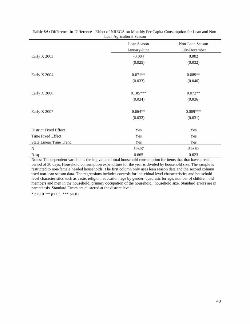
40

Table 8A: Difference-in-Difference - Effect of NREGA on Monthly Per Capita Consumption for Lean and Non-

Lean Agricultural Season

Lean Season Non-Lean Season

January-June July-December

Early X 2003 -0.004 0.002

(0.025) (0.032)

Early X 2004 0.071** 0.089**

(0.033) (0.040)

Early X 2006 0.105*** 0.072**

(0.034) (0.036)

Early X 2007 0.064** 0.089***

(0.032) (0.031)

District Fixed Effect Yes Yes

Time Fixed Effect Yes Yes

State Linear Time Trend Yes Yes

N 59397 59360

R-sq 0.665 0.623

Notes: The dependent variable is the log value of total household consumption for items that that have a recall

period of 30 days. Household consumption expenditure for the year is divided by household size. The sample is

restricted to non-female headed households. The first column only uses lean season data and the second column

used non-lean season data. The regressions includes controls for individual level characteristics and household

level characteristics such as caste, religion, education, age by gender, quadratic for age, number of children, old

members and men in the household, primary occupation of the household, household size. Standard errors are in

parenthesis. Standard Errors are clustered at the district level.

* p<.10 ** p<.05 *** p<.01

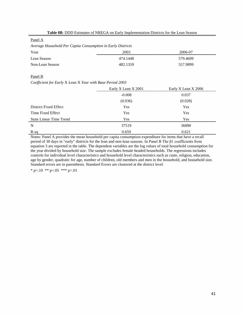
41

Table 8B: DDD Estimates of NREGA on Early Implementation Districts for the Lean Season

Panel A

Average Household Per Capita Consumption in Early Districts

Year 2003 2006-07

Lean Season 474.1448 579.4609

Non-Lean Season 482.1359 557.9899

Panel B

Coefficient for Early X Lean X Year with Base Period 2003

Early X Lean X 2001 Early X Lean X 2006

-0.008 0.037

(0.036) (0.028)

District Fixed Effect Yes Yes

Time Fixed Effect Yes Yes

State Linear Time Trend Yes Yes

N 37519 36890

R-sq 0.659 0.621

Notes: Panel A provides the mean household per capita consumption expenditure for items that have a recall

period of 30 days in "early" districts for the lean and non-lean seasons. In Panel B The β1 coefficients from

equation 3 are reported in the table. The dependent variables are the log values of total household consumption for

the year divided by household size. The sample excludes female headed households. The regressions includes

controls for individual level characteristics and household level characteristics such as caste, religion, education,

age by gender, quadratic for age, number of children, old members and men in the household, and household size.

Standard errors are in parenthesis. Standard Errors are clustered at the district level.

* p<.10 ** p<.05 *** p<.01

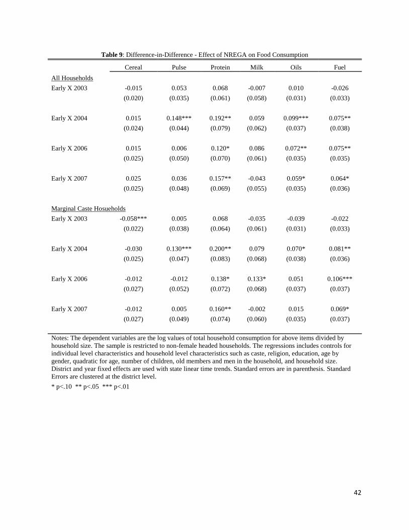
42

Table 9: Difference-in-Difference - Effect of NREGA on Food Consumption

Cereal Pulse Protein Milk Oils Fuel

All Households

Early X 2003 -0.015 0.053 0.068 -0.007 0.010 -0.026

(0.020) (0.035) (0.061) (0.058) (0.031) (0.033)

Early X 2004 0.015 0.148*** 0.192** 0.059 0.099*** 0.075**

(0.024) (0.044) (0.079) (0.062) (0.037) (0.038)

Early X 2006 0.015 0.006 0.120* 0.086 0.072** 0.075**

(0.025) (0.050) (0.070) (0.061) (0.035) (0.035)

Early X 2007 0.025 0.036 0.157** -0.043 0.059* 0.064*

(0.025) (0.048) (0.069) (0.055) (0.035) (0.036)

Marginal Caste Hosueholds

Early X 2003 -0.058*** 0.005 0.068 -0.035 -0.039 -0.022

(0.022) (0.038) (0.064) (0.061) (0.031) (0.033)

Early X 2004 -0.030 0.130*** 0.200** 0.079 0.070* 0.081**

(0.025) (0.047) (0.083) (0.068) (0.038) (0.036)

Early X 2006 -0.012 -0.012 0.138* 0.133* 0.051 0.106***

(0.027) (0.052) (0.072) (0.068) (0.037) (0.037)

Early X 2007 -0.012 0.005 0.160** -0.002 0.015 0.069*

(0.027) (0.049) (0.074) (0.060) (0.035) (0.037)

Notes: The dependent variables are the log values of total household consumption for above items divided by

household size. The sample is restricted to non-female headed households. The regressions includes controls for

individual level characteristics and household level characteristics such as caste, religion, education, age by

gender, quadratic for age, number of children, old members and men in the household, and household size.

District and year fixed effects are used with state linear time trends. Standard errors are in parenthesis. Standard

Errors are clustered at the district level.

* p<.10 ** p<.05 *** p<.01

43

Table 10: Difference-in-Difference - Effect of NREGA on Education and Health

Education Intoxicants Tobacco Beverage Medical

Medical

(Institutional)

All Households

Early X 2003 -0.098 -0.100 0.072 -0.013 -0.025 -0.097

(0.089) (0.096) (0.056) (0.057) (0.082) (0.156)

Early X 2004 -0.020 0.021 0.079 0.154** -0.028 0.008

(0.091) (0.112) (0.070) (0.063) (0.102) (0.185)

Early X 2006 0.028 0.137 0.107 0.160** 0.049 0.123

(0.097) (0.123) (0.077) (0.068) (0.084) (0.198)

Early X 2007 0.021 0.208* 0.118 0.132* 0.044 0.120

(0.092) (0.124) (0.079) (0.068) (0.094) (0.202)

Marginal Caste Hosueholds

Early X 2003 -0.122 -0.117 0.058 -0.094 0.037 -0.094

(0.095) (0.103) (0.061) (0.058) (0.095) (0.170)

Early X 2004 -0.008 0.035 0.106 0.124* 0.057 0.023

(0.102) (0.122) (0.069) (0.065) (0.104) (0.195)

Early X 2006 0.026 0.090 0.099 0.120* 0.159 0.114

(0.111) (0.128) (0.084) (0.071) (0.104) (0.222)

Early X 2007 0.028 0.152 0.103 0.094 0.148 0.078

(0.107) (0.125) (0.084) (0.073) (0.106) (0.231)

Notes: The dependent variables are the log values of total household consumption for above items divided by

household size. The sample is restricted to non-female headed households. The regressions includes controls for

individual level characteristics and household level characteristics such as caste, religion, education, age by

gender, quadratic for age, number of children, old members and men in the household, and household size.

District and year fixed effects are used with state linear time trends. Standard errors are in parenthesis. Standard

Errors are clustered at the district level.

* p<.10 ** p<.05 *** p<.01

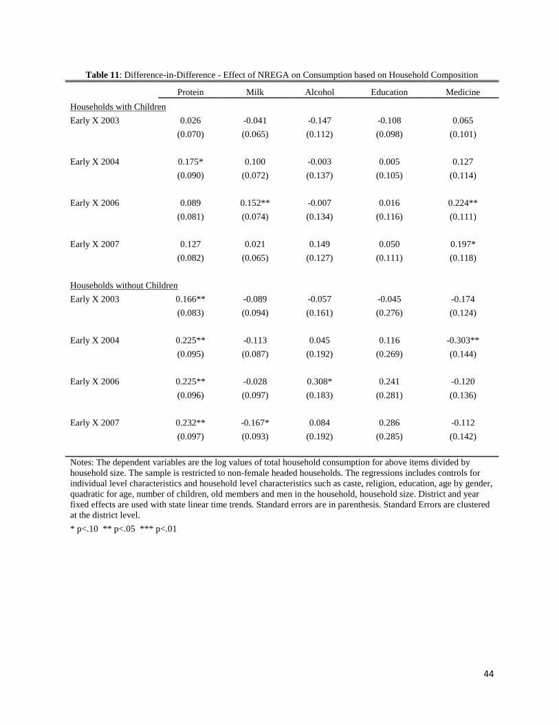
44

Table 11: Difference-in-Difference - Effect of NREGA on Consumption based on Household Composition

Protein Milk Alcohol Education Medicine

Households with Children

Early X 2003 0.026 -0.041 -0.147 -0.108 0.065

(0.070) (0.065) (0.112) (0.098) (0.101)

Early X 2004 0.175* 0.100 -0.003 0.005 0.127

(0.090) (0.072) (0.137) (0.105) (0.114)

Early X 2006 0.089 0.152** -0.007 0.016 0.224**

(0.081) (0.074) (0.134) (0.116) (0.111)

Early X 2007 0.127 0.021 0.149 0.050 0.197*

(0.082) (0.065) (0.127) (0.111) (0.118)

Households without Children

Early X 2003 0.166** -0.089 -0.057 -0.045 -0.174

(0.083) (0.094) (0.161) (0.276) (0.124)

Early X 2004 0.225** -0.113 0.045 0.116 -0.303**

(0.095) (0.087) (0.192) (0.269) (0.144)

Early X 2006 0.225** -0.028 0.308* 0.241 -0.120

(0.096) (0.097) (0.183) (0.281) (0.136)

Early X 2007 0.232** -0.167* 0.084 0.286 -0.112

(0.097) (0.093) (0.192) (0.285) (0.142)

Notes: The dependent variables are the log values of total household consumption for above items divided by

household size. The sample is restricted to non-female headed households. The regressions includes controls for

individual level characteristics and household level characteristics such as caste, religion, education, age by gender,

quadratic for age, number of children, old members and men in the household, household size. District and year

fixed effects are used with state linear time trends. Standard errors are in parenthesis. Standard Errors are clustered

at the district level.

* p<.10 ** p<.05 *** p<.01

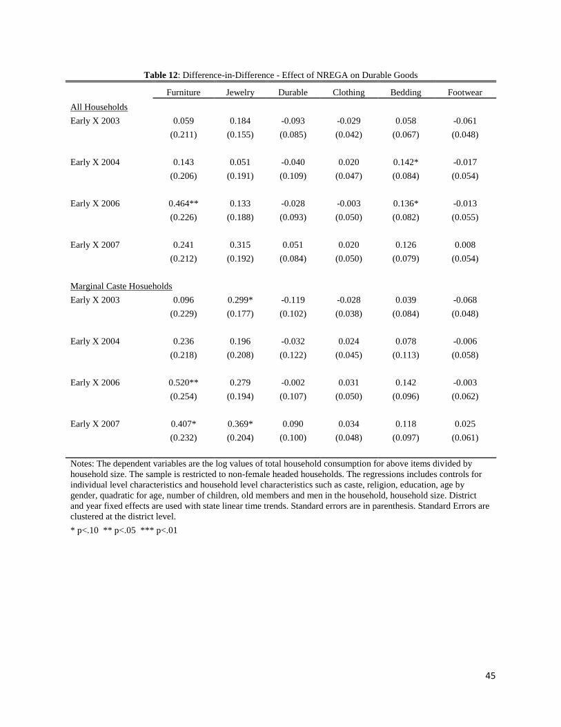
45

Table 12: Difference-in-Difference - Effect of NREGA on Durable Goods

Furniture Jewelry Durable Clothing Bedding Footwear

All Households

Early X 2003 0.059 0.184 -0.093 -0.029 0.058 -0.061

(0.211) (0.155) (0.085) (0.042) (0.067) (0.048)

Early X 2004 0.143 0.051 -0.040 0.020 0.142* -0.017

(0.206) (0.191) (0.109) (0.047) (0.084) (0.054)

Early X 2006 0.464** 0.133 -0.028 -0.003 0.136* -0.013

(0.226) (0.188) (0.093) (0.050) (0.082) (0.055)

Early X 2007 0.241 0.315 0.051 0.020 0.126 0.008

(0.212) (0.192) (0.084) (0.050) (0.079) (0.054)

Marginal Caste Hosueholds

Early X 2003 0.096 0.299* -0.119 -0.028 0.039 -0.068

(0.229) (0.177) (0.102) (0.038) (0.084) (0.048)

Early X 2004 0.236 0.196 -0.032 0.024 0.078 -0.006

(0.218) (0.208) (0.122) (0.045) (0.113) (0.058)

Early X 2006 0.520** 0.279 -0.002 0.031 0.142 -0.003

(0.254) (0.194) (0.107) (0.050) (0.096) (0.062)

Early X 2007 0.407* 0.369* 0.090 0.034 0.118 0.025

(0.232) (0.204) (0.100) (0.048) (0.097) (0.061)

Notes: The dependent variables are the log values of total household consumption for above items divided by

household size. The sample is restricted to non-female headed households. The regressions includes controls for

individual level characteristics and household level characteristics such as caste, religion, education, age by

gender, quadratic for age, number of children, old members and men in the household, household size. District

and year fixed effects are used with state linear time trends. Standard errors are in parenthesis. Standard Errors are

clustered at the district level.

* p<.10 ** p<.05 *** p<.01