Ray-tracing and other Rendering Approaches

2

What happens in Nature• In nature, a light source emits a ray of light which travels, eventually, to a surface that interrupts its

progress.

• This "ray" is a stream of photons travelling along the same path. In a perfect vacuum this ray will be a straight line.

• When the ray hits a surface three things happen

• absorption, reflection, and refraction.

• A surface may reflect all or part of the light ray, in one or more directions.

• It might also absorb part of the light ray, resulting in a loss of intensity of the light

• If the surface has any transparent or translucent properties, it refracts a portion of the light beam into itself in a different direction while absorbing some (or all) of the spectrum (and possibly altering the colour)

• These different amounts must sum to unity (conservation of energy)

3

Raytracing

•Rene Descartes introduced ray tracing back in 1637 – the idea of tracing(or plotting) light rays and their interaction between surfaces.

•He applied the laws of refraction and reflection to a spherical water droplet to demonstrate the formation of rainbows.

4

Ray-casting• The first ray casting algorithm used for rendering was presented by Arthur Appel in 1968.

• The idea behind ray casting is to shoot rays from the eye, one per pixel, and find the closest object blocking the path of that ray

• Using the material properties and the effect of the lights in the scene, this algorithm can determine the shading of this object.

• The simplifying assumption is made that if a surface faces a light, the light will reach that surface and not be blocked or in shadow.

• The shading of the surface is computed using traditional 3D computer graphics shading models.

• One important advantage ray casting offered over older scanline algorithms is its ability to easily deal with non-planar surfaces and solids

• If a mathematical surface can be intersected by a ray, it can be rendered using ray casting. Elaborate objects can be created by using solid modeling techniques and easily rendered.

5

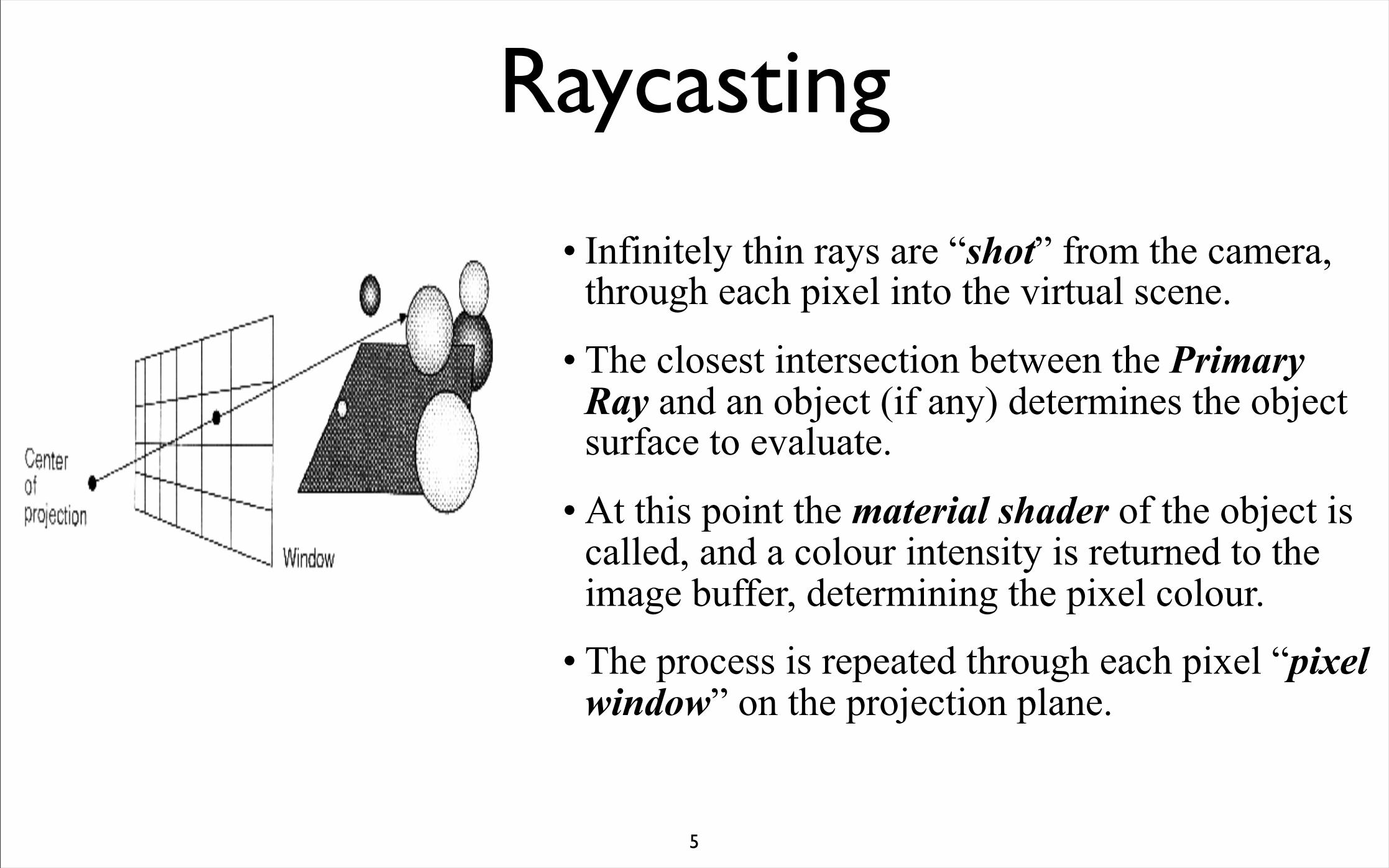
Raycasting

• Infinitely thin rays are “shot” from the camera, through each pixel into the virtual scene.

• The closest intersection between the Primary Ray and an object (if any) determines the object surface to evaluate.

• At this point the material shader of the object is called, and a colour intensity is returned to the image buffer, determining the pixel colour.

• The process is repeated through each pixel “pixel window” on the projection plane.

6

Raytracing• Turner Whitted (1979) Used the basic ray casting algorithm but extended it

• When a ray hits a surface, it could generate up to three new types of rays:

• reflection, refraction, and shadow.

• A reflected ray continues on in the mirror-reflection direction from a shiny surface.

• It is then intersected with objects in the scene; the closest object it intersects is what will be seen in the reflection.

• Refraction rays travelling through transparent material work similarly, with the addition that a refractive ray could be entering or exiting a material.

• To further avoid tracing all rays in a scene, a shadow ray is used to test if a surface is visible to a light.

• A ray hits a surface at some point. If the surface at this point faces a light, a ray (to the computer, a line segment) is traced between this intersection point and the light.

7

Ray Tracing Renderers•Ray tracing approximates properties of light to determine pixel colour intensity.

•As such, thousands of calculations need to be generated to determine every pixel colour.

•Ray tracing does NOT project all objects onto the projection plane – it deals with objects in 3D space.

•Ray Tracing does use the projection plane to determine the direction from which to “shoot” rays.

8

Raytracing Advantages

• Realistic simulation of lighting (better than scanline rendering or ray casting).

• Effects such as reflections and shadows, which are difficult to simulate using other algorithms, are a natural result of the ray tracing algorithm.

• Relatively simple to implement yet yielding impressive visual results

9

Raytracing Disadvantages• Performance is very poor.

• Scanline algorithms and other algorithms use data coherence to share computations between pixels, while ray tracing normally starts the process anew, treating each eye ray separately.

• However, this separation offers other advantages, such as the ability to shoot more rays as needed to perform anti-aliasing and improve image quality where needed. Although it does handle inter-reflection and optical effects such as refraction accurately.

• Other methods, including photon mapping, are based upon ray tracing for certain parts of the algorithm, yet give far better results.

10

Efficiency•Like the visible surface algorithms, ray tracing can use an incredible amount of calculations to determine the correct object intersection.

•An image 1024 x 1024, with 100 objects would require over 100,000,000 calculations just to define the correct objects and the relevant intersection points.

•For each pixel we still require the necessary additional calculations that determine the actual colour intensity.

•Early ray tracing techniques ( e.g. Whitted in 1980) discovered that around 75% – 95% of the actual ray tracing algorithm was spent in generating intersection calculations.

•Several options were advanced to solve these problems.

•Some lay in the actual maths - adjustments to make certain intersections that repeat easily resolve.

11

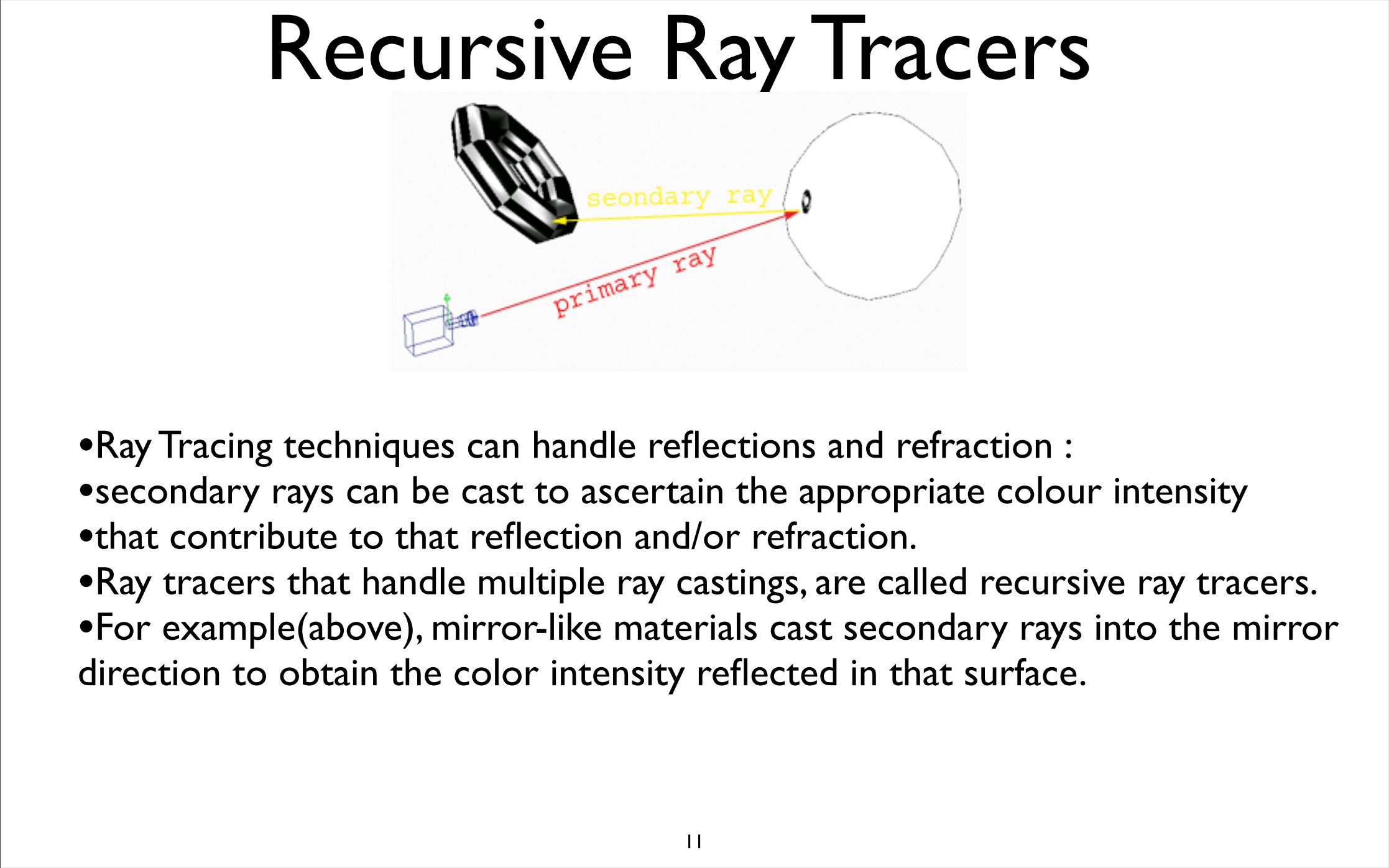
Recursive Ray Tracers

•Ray Tracing techniques can handle reflections and refraction :•secondary rays can be cast to ascertain the appropriate colour intensity •that contribute to that reflection and/or refraction.•Ray tracers that handle multiple ray castings, are called recursive ray tracers.•For example(above), mirror-like materials cast secondary rays into the mirror direction to obtain the color intensity reflected in that surface.

12

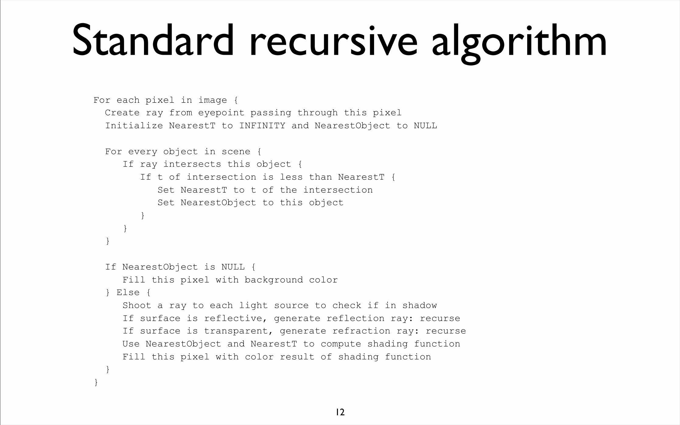
Standard recursive algorithmFor each pixel in image { Create ray from eyepoint passing through this pixel Initialize NearestT to INFINITY and NearestObject to NULL

For every object in scene { If ray intersects this object { If t of intersection is less than NearestT { Set NearestT to t of the intersection Set NearestObject to this object } } }

If NearestObject is NULL { Fill this pixel with background color } Else { Shoot a ray to each light source to check if in shadow If surface is reflective, generate reflection ray: recurse If surface is transparent, generate refraction ray: recurse Use NearestObject and NearestT to compute shading function Fill this pixel with color result of shading function }}

13

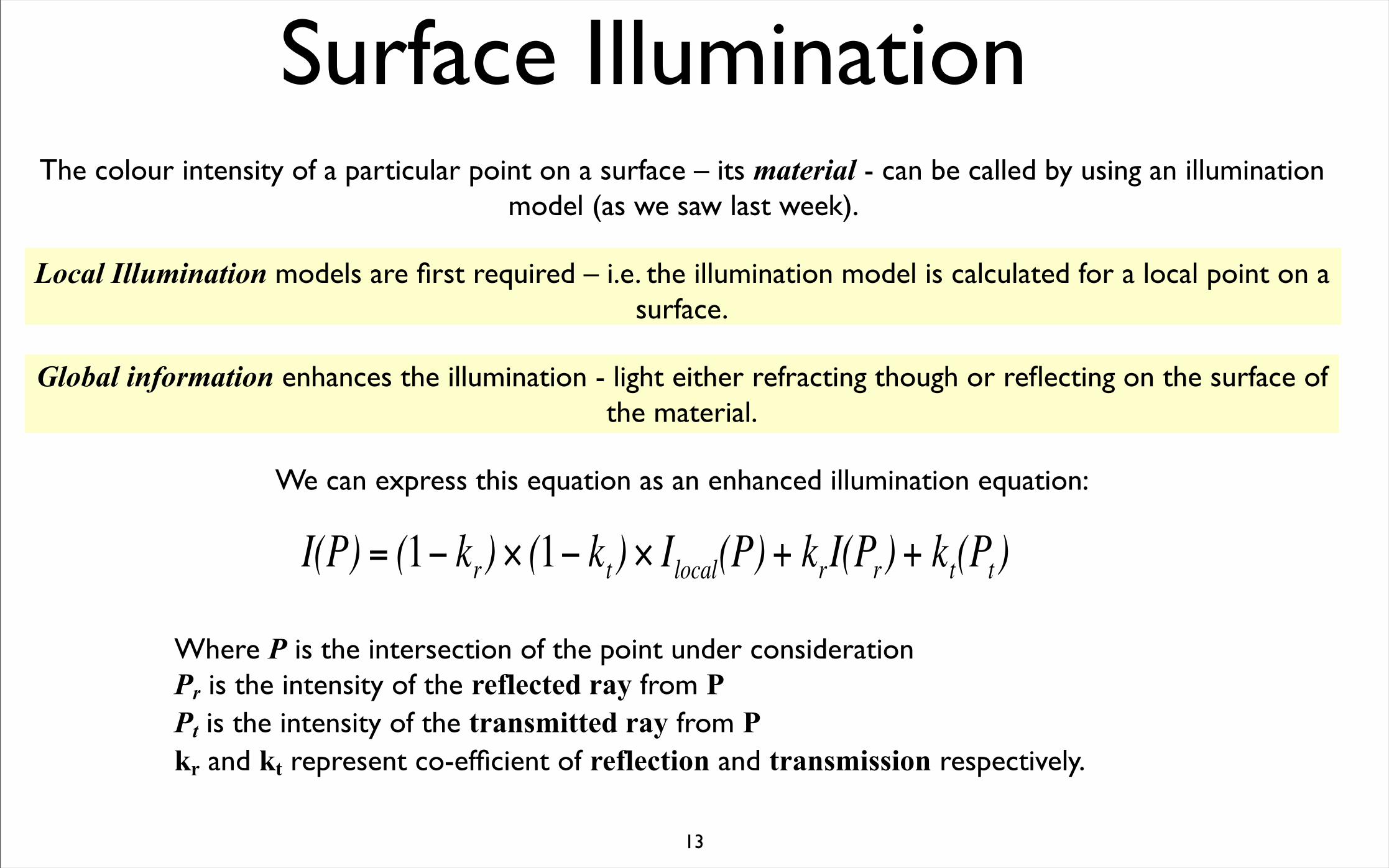
Surface IlluminationThe colour intensity of a particular point on a surface – its material - can be called by using an illumination

model (as we saw last week).

Local Illumination models are first required – i.e. the illumination model is calculated for a local point on a surface.

Global information enhances the illumination - light either refracting though or reflecting on the surface of the material.

We can express this equation as an enhanced illumination equation:

€

I(P) = (1− kr) × (1− kt) × Ilocal(P) + krI(Pr) + kt(Pt)

Where P is the intersection of the point under considerationPr is the intensity of the reflected ray from PPt is the intensity of the transmitted ray from Pkr and kt represent co-efficient of reflection and transmission respectively.

14

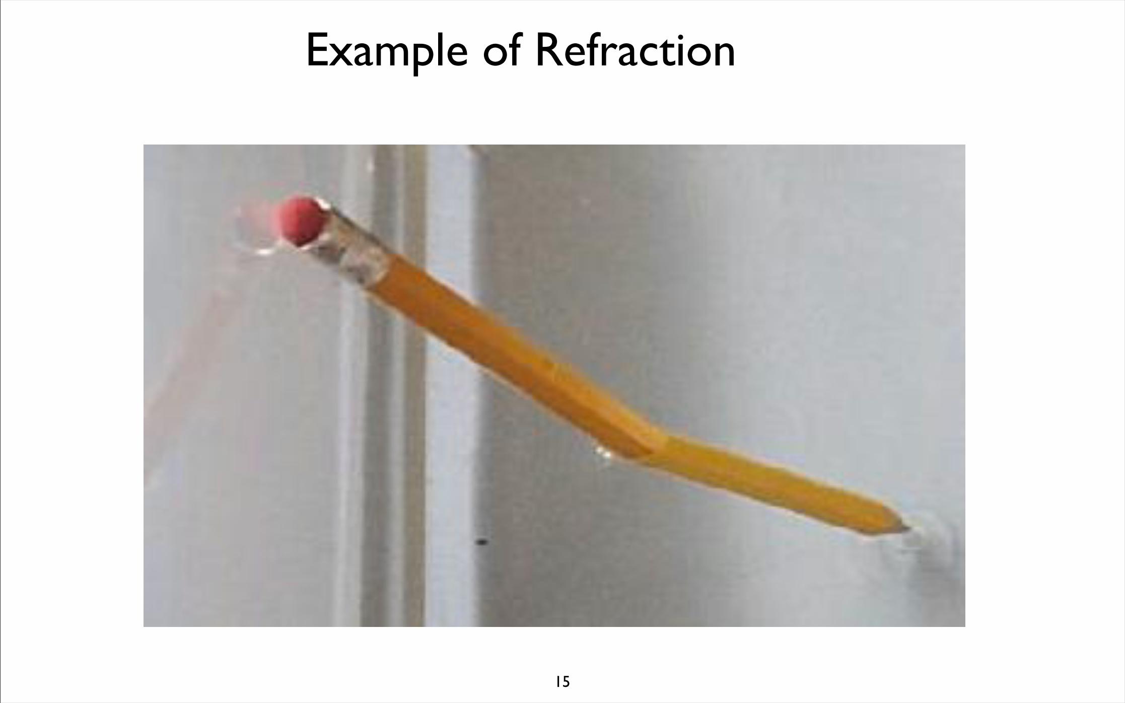
Transparency, Reflections and Refraction

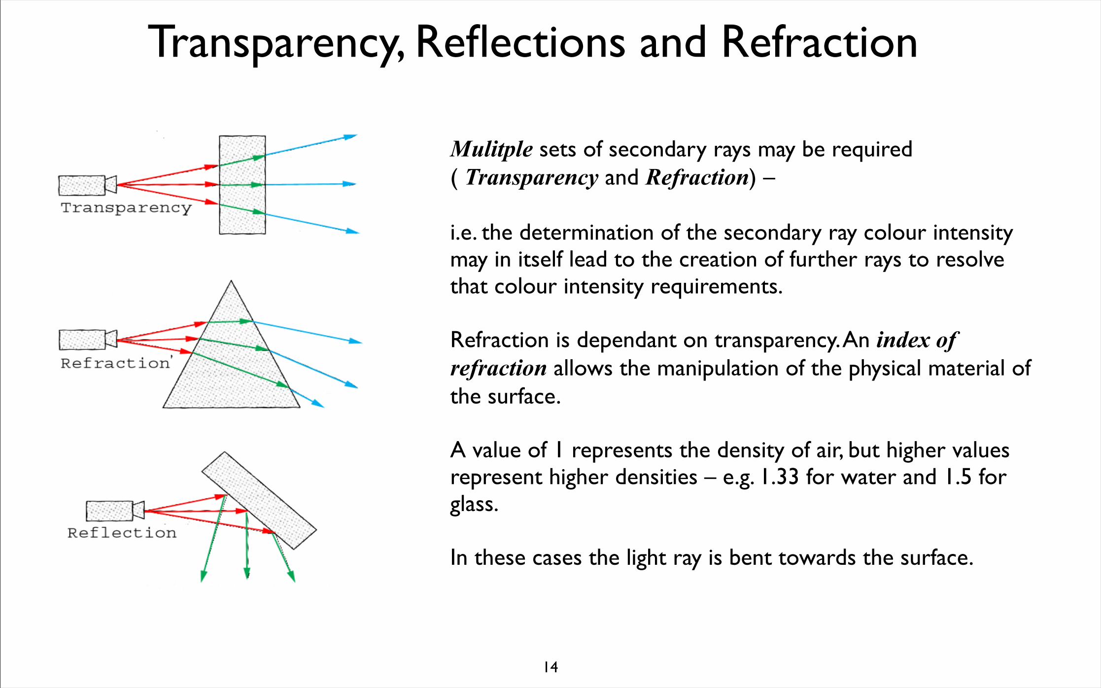
Mulitple sets of secondary rays may be required ( Transparency and Refraction) –

i.e. the determination of the secondary ray colour intensity may in itself lead to the creation of further rays to resolve that colour intensity requirements.

Refraction is dependant on transparency. An index of refraction allows the manipulation of the physical material of the surface.

A value of 1 represents the density of air, but higher values represent higher densities – e.g. 1.33 for water and 1.5 for glass.

In these cases the light ray is bent towards the surface.

15

Example of Refraction

16

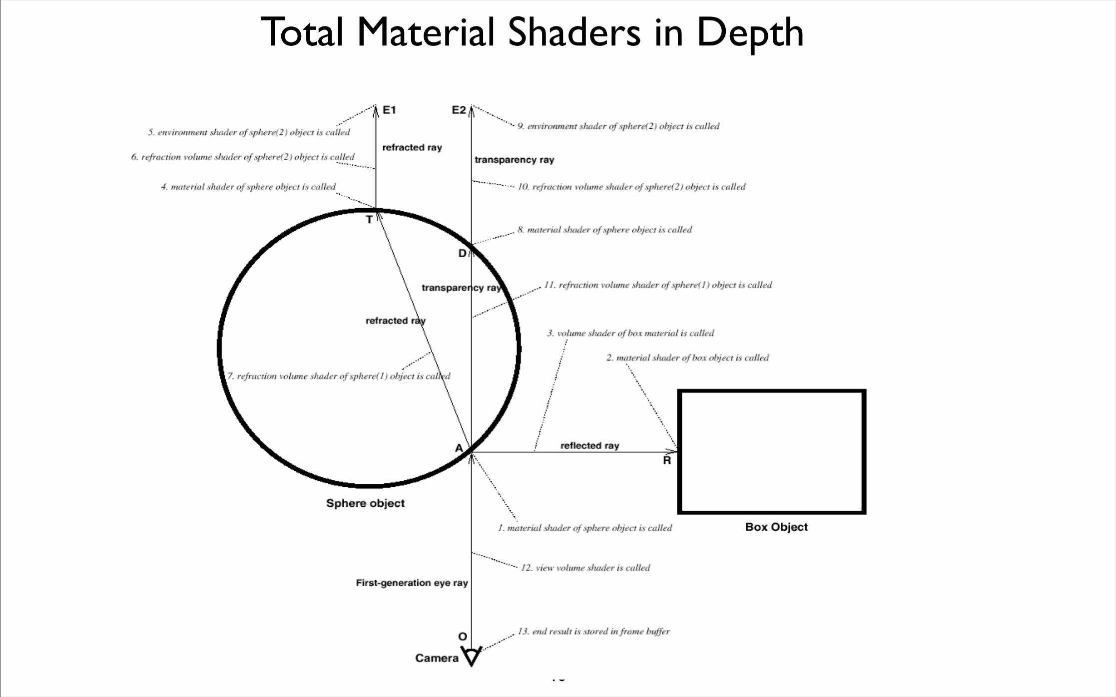
Total Material Shaders in Depth

17

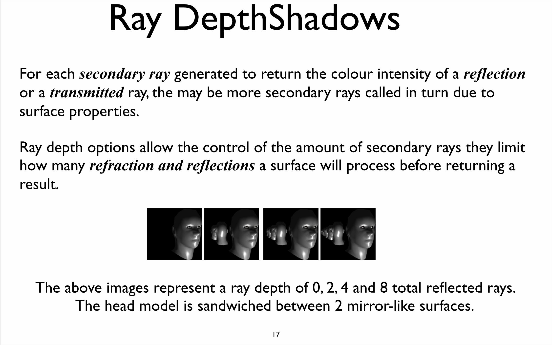
Ray DepthShadowsFor each secondary ray generated to return the colour intensity of a reflection or a transmitted ray, the may be more secondary rays called in turn due to surface properties.

Ray depth options allow the control of the amount of secondary rays they limit how many refraction and reflections a surface will process before returning a result.

The above images represent a ray depth of 0, 2, 4 and 8 total reflected rays. The head model is sandwiched between 2 mirror-like surfaces.

18

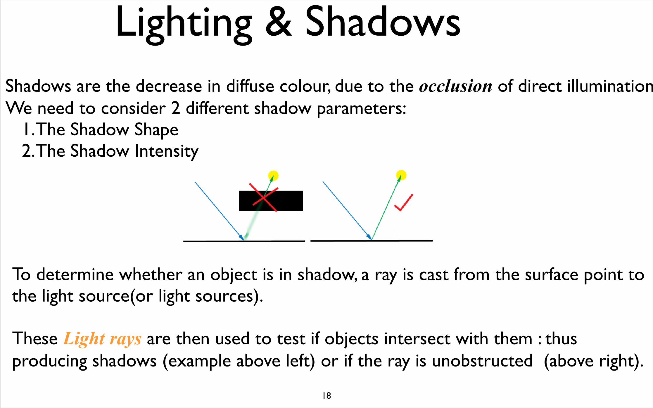
Lighting & ShadowsShadows are the decrease in diffuse colour, due to the occlusion of direct illumination.We need to consider 2 different shadow parameters:

1.The Shadow Shape2.The Shadow Intensity

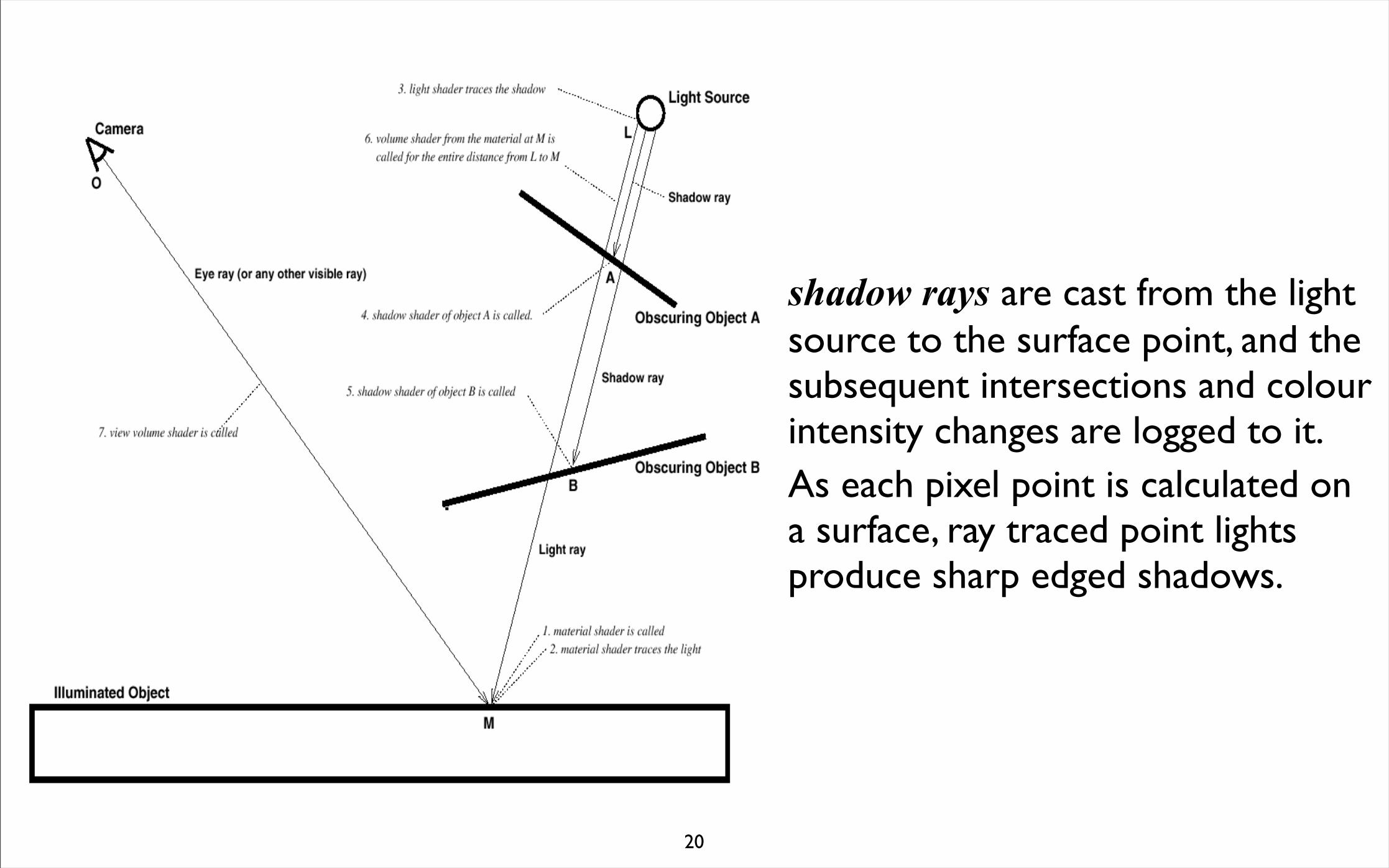
To determine whether an object is in shadow, a ray is cast from the surface point to the light source(or light sources).

These Light rays are then used to test if objects intersect with them : thus producing shadows (example above left) or if the ray is unobstructed (above right).

19

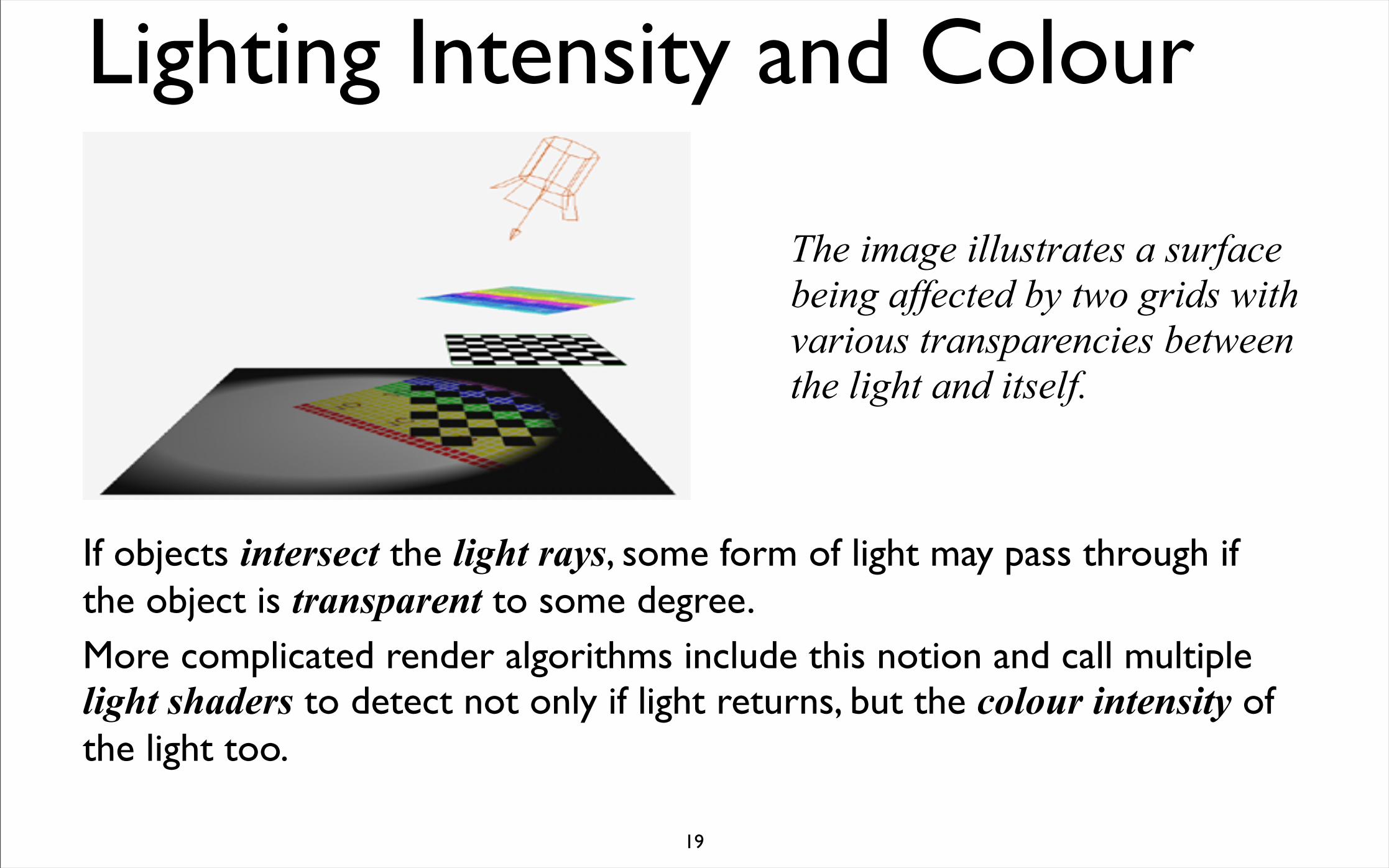
Lighting Intensity and Colour

If objects intersect the light rays, some form of light may pass through if the object is transparent to some degree. More complicated render algorithms include this notion and call multiple light shaders to detect not only if light returns, but the colour intensity of the light too.

The image illustrates a surface being affected by two grids with various transparencies between the light and itself.

20

shadow rays are cast from the light source to the surface point, and the subsequent intersections and colour intensity changes are logged to it.As each pixel point is calculated on a surface, ray traced point lights produce sharp edged shadows.

21

22

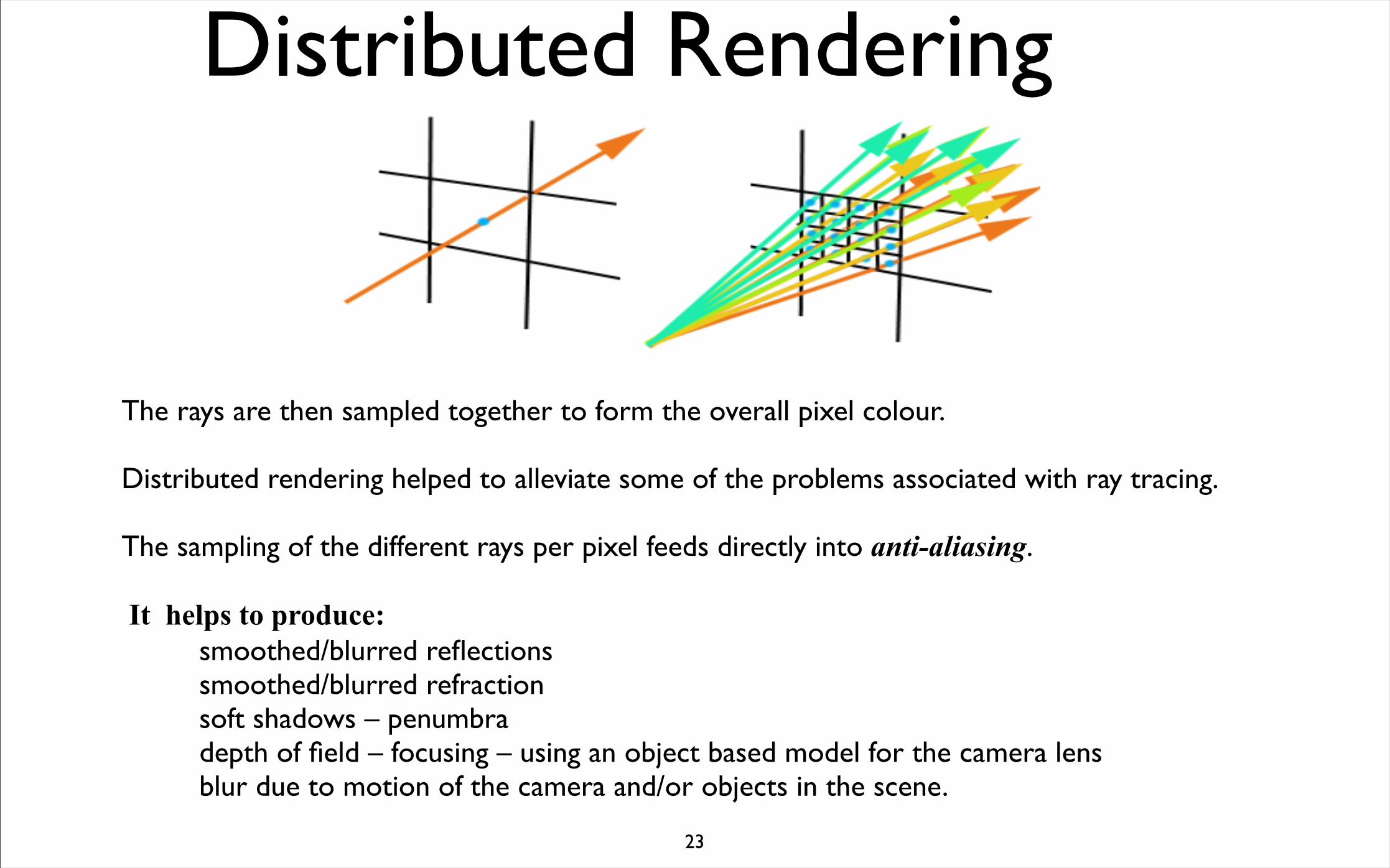
Super Real RendersBasic recursive ray tracers produce what is commonly referred to as “super real” images.

This signature of ray tracers is as follows:

‘sharp’ shadows‘sharp’ reflections‘sharp’ refractions

lack of diffuse interaction between surfaces –radiosity of light lack of caustics – the refraction and reflection of specular highlights

One method of overcoming these problems is to increase the sampling of the pixel area.

The pixel space on the projection plane (a single hole) is be broken down into smaller windows – 4 x 4 for example.

A ray is fired through every sub-region – in some cases a random position inside that region.

Although computationally much more expensive, this approach does help ray tracing on many level. This form of ray tracing is known as distributed rendering.

23

Distributed Rendering

The rays are then sampled together to form the overall pixel colour.

Distributed rendering helped to alleviate some of the problems associated with ray tracing.

The sampling of the different rays per pixel feeds directly into anti-aliasing.

It helps to produce: smoothed/blurred reflections smoothed/blurred refraction soft shadows – penumbra depth of field – focusing – using an object based model for the camera lens blur due to motion of the camera and/or objects in the scene.

24

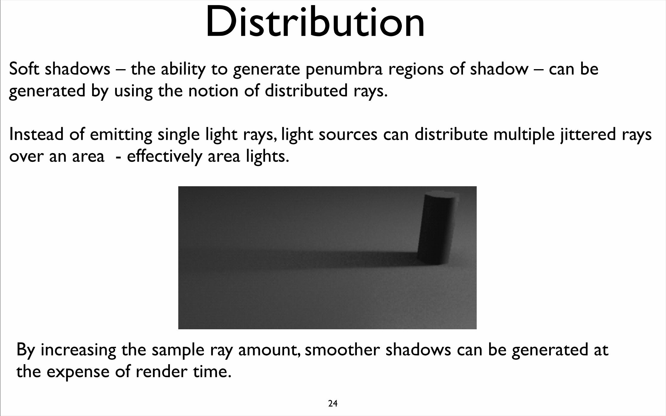
DistributionSoft shadows – the ability to generate penumbra regions of shadow – can be generated by using the notion of distributed rays.

Instead of emitting single light rays, light sources can distribute multiple jittered rays over an area - effectively area lights.

By increasing the sample ray amount, smoother shadows can be generated at the expense of render time.

25

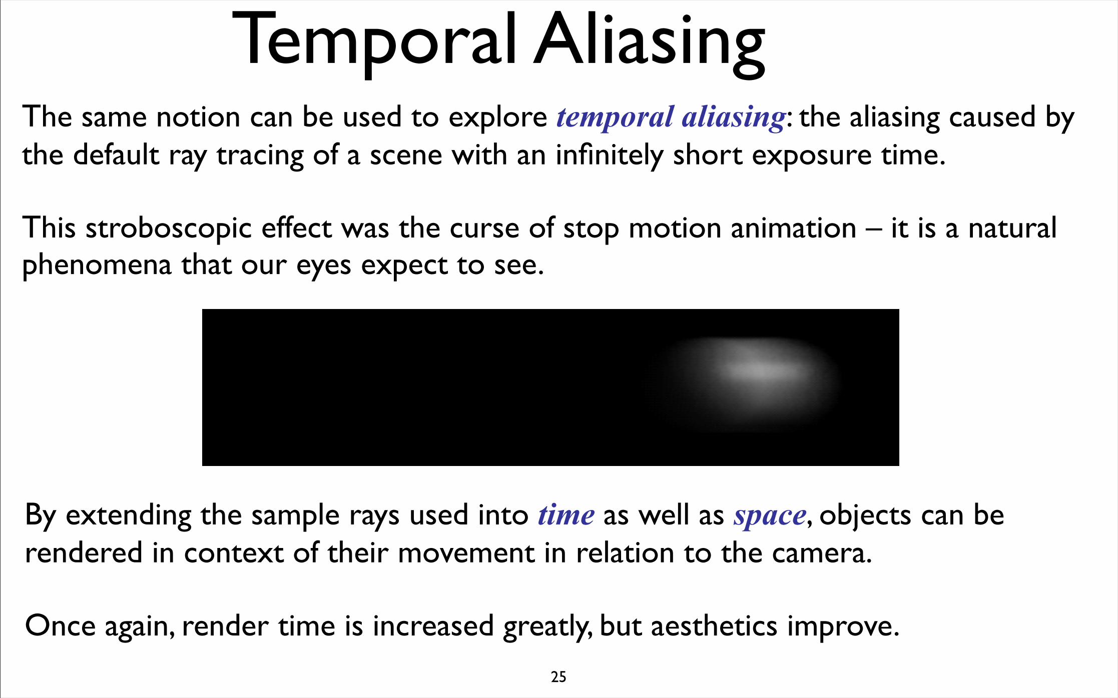
Temporal AliasingThe same notion can be used to explore temporal aliasing: the aliasing caused by the default ray tracing of a scene with an infinitely short exposure time.

This stroboscopic effect was the curse of stop motion animation – it is a natural phenomena that our eyes expect to see.

By extending the sample rays used into time as well as space, objects can be rendered in context of their movement in relation to the camera.

Once again, render time is increased greatly, but aesthetics improve.

26

Monte-Carlo RayTracing

•This is an common name referring to Ray-Tracing which uses random numbers to sample unknown quantities.

•Glossy reflection, refractions, occlusions, distributed rendering of pixels, global illumination, sub-surface-scattering etc are all capable in a Monte-Carlo ray tracer.

•Samples are summed and then averaged to gain the desired result, usually to determine pixel colour.

27

2 Pass Ray Tracing•Distributed rendering helps to solve problems but some of the major aesthetic problems still persist:diffuse interaction > the bleeding of diffuse colour from surface to surface.specular refraction & projection > the illumination of surfaces via specular

reflection

•These problems lead to the next generation of ray tracers.•These are called 2 Pass Ray Tracers – named because they mix forward ray tracing and backward ray tracing.•The notion of forward and backwards is subject to dispute:•Normal ray tracers interpret rays from the eye to the surface(opposite of reality). •Backwards (or forwards!?) ray tracers process light from the light to surfaces.•Forwards and backwards …2 Pass Ray Tracers utilise both techniques…

28

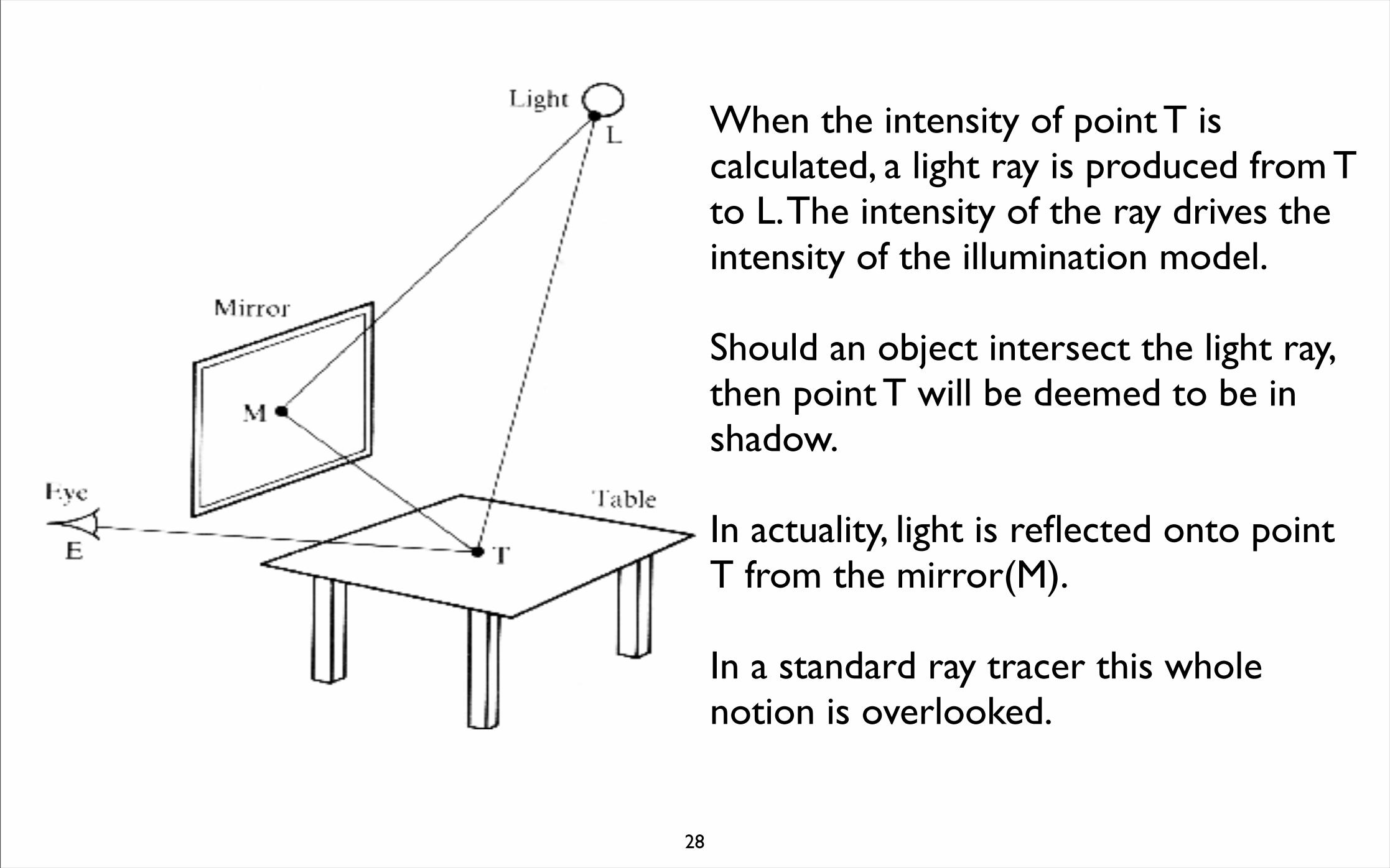
When the intensity of point T is calculated, a light ray is produced from T to L. The intensity of the ray drives the intensity of the illumination model.

Should an object intersect the light ray, then point T will be deemed to be in shadow.

In actuality, light is reflected onto point T from the mirror(M).

In a standard ray tracer this whole notion is overlooked.

29

Local & Global 2 Pass•2 Pass ray tracers basically combine local and global illuminations.

•They are used to incorporate the specular reflection into illumination.

•They work by combining a standard illumination with a global illumination- simply by adding the two together.

•i.e. Local illumination (phong, etc.) + any extraneous global light.

• Global illumination usually has its own coefficient - commonly termed “irradiance”.

30

Step1

Rays are fired from the light source and are followed until they hit a diffuse surface.

The light energy is then cached into that surface, which is subdivided enough to incorporate subtle changes in colour without blurring or graininess.

This is known as an illumination map.

Step 2

Normal Whitted ray tracing.

Geometry Approach

31

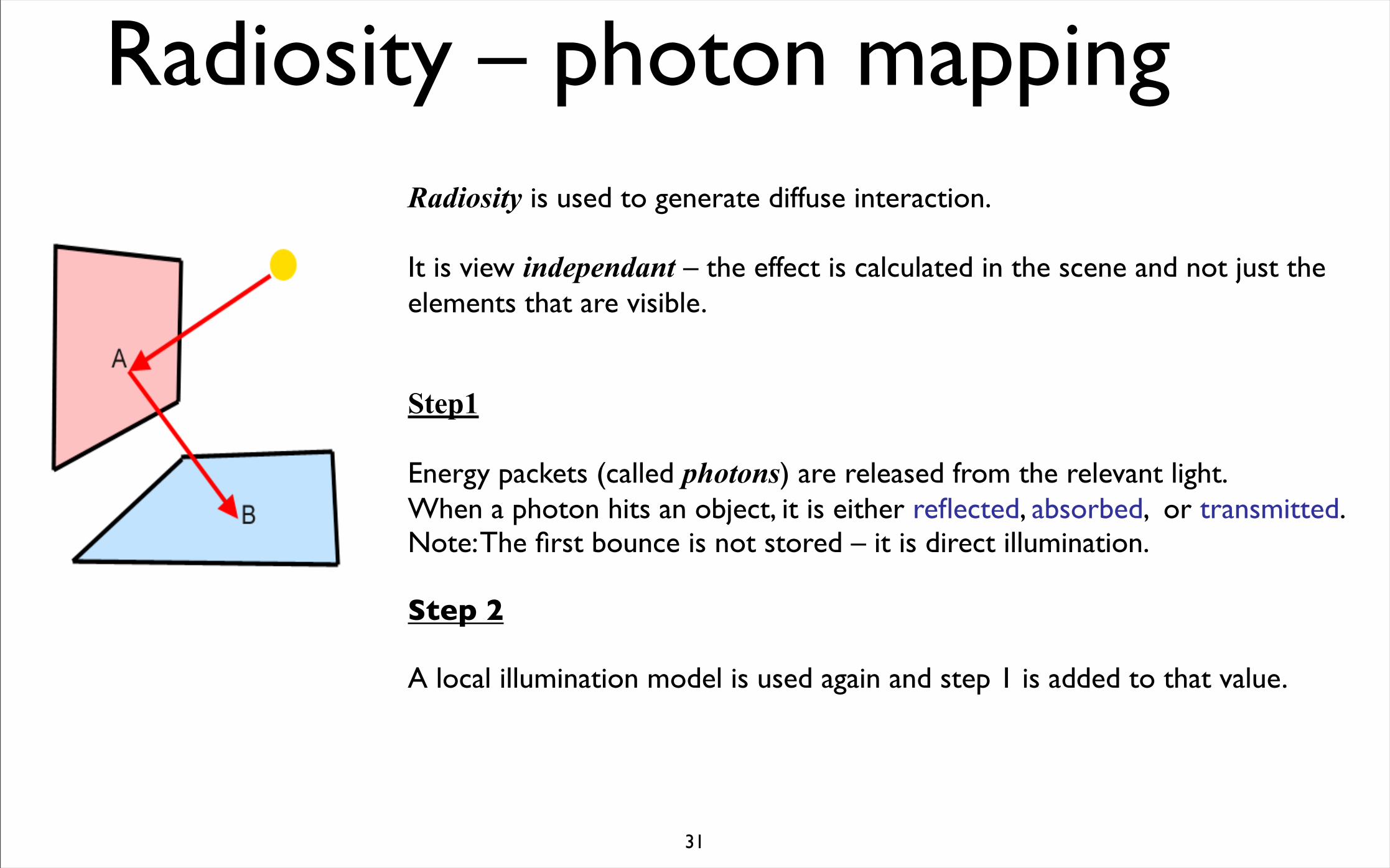
Radiosity – photon mappingRadiosity is used to generate diffuse interaction.

It is view independant – the effect is calculated in the scene and not just the elements that are visible.

Step1

Energy packets (called photons) are released from the relevant light.When a photon hits an object, it is either reflected, absorbed, or transmitted.Note: The first bounce is not stored – it is direct illumination.

Step 2

A local illumination model is used again and step 1 is added to that value.

32

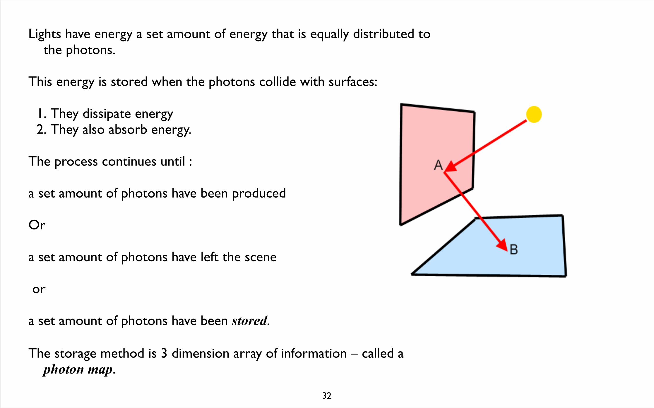
Lights have energy a set amount of energy that is equally distributed to the photons.

This energy is stored when the photons collide with surfaces:

1. They dissipate energy 2. They also absorb energy.

The process continues until :

a set amount of photons have been produced

Or

a set amount of photons have left the scene

or

a set amount of photons have been stored.

The storage method is 3 dimension array of information – called a photon map.

33

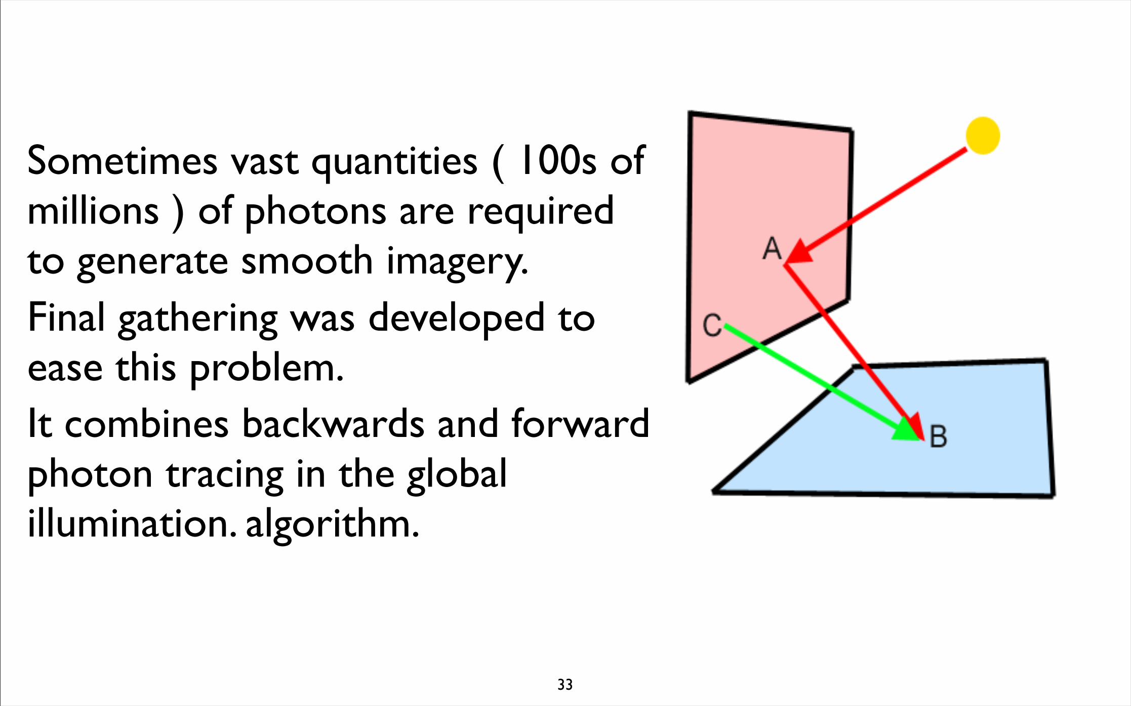
Sometimes vast quantities ( 100s of millions ) of photons are required to generate smooth imagery.Final gathering was developed to ease this problem. It combines backwards and forward photon tracing in the global illumination. algorithm.

34

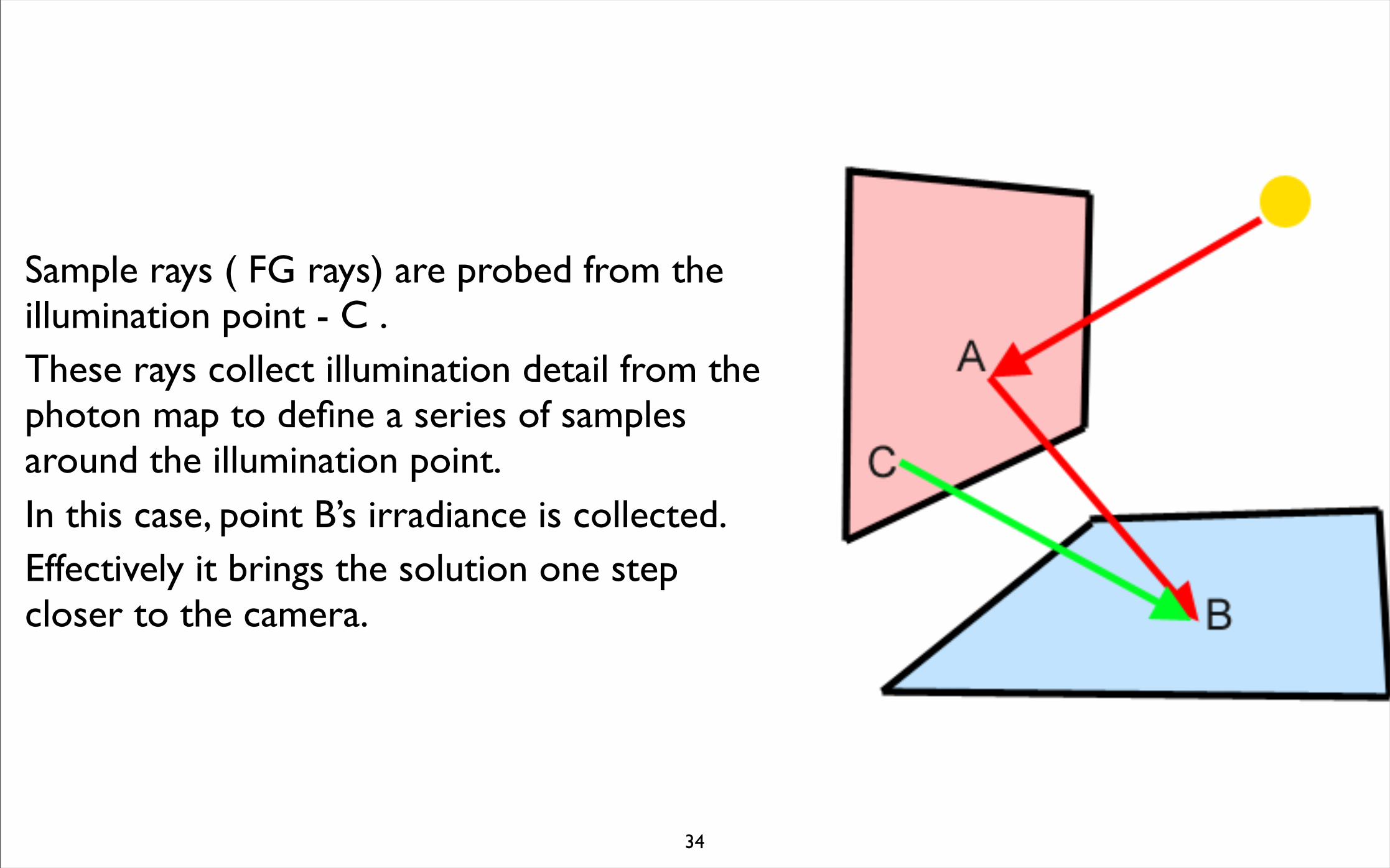
Sample rays ( FG rays) are probed from the illumination point - C .These rays collect illumination detail from the photon map to define a series of samples around the illumination point.In this case, point B’s irradiance is collected.Effectively it brings the solution one step closer to the camera.

35

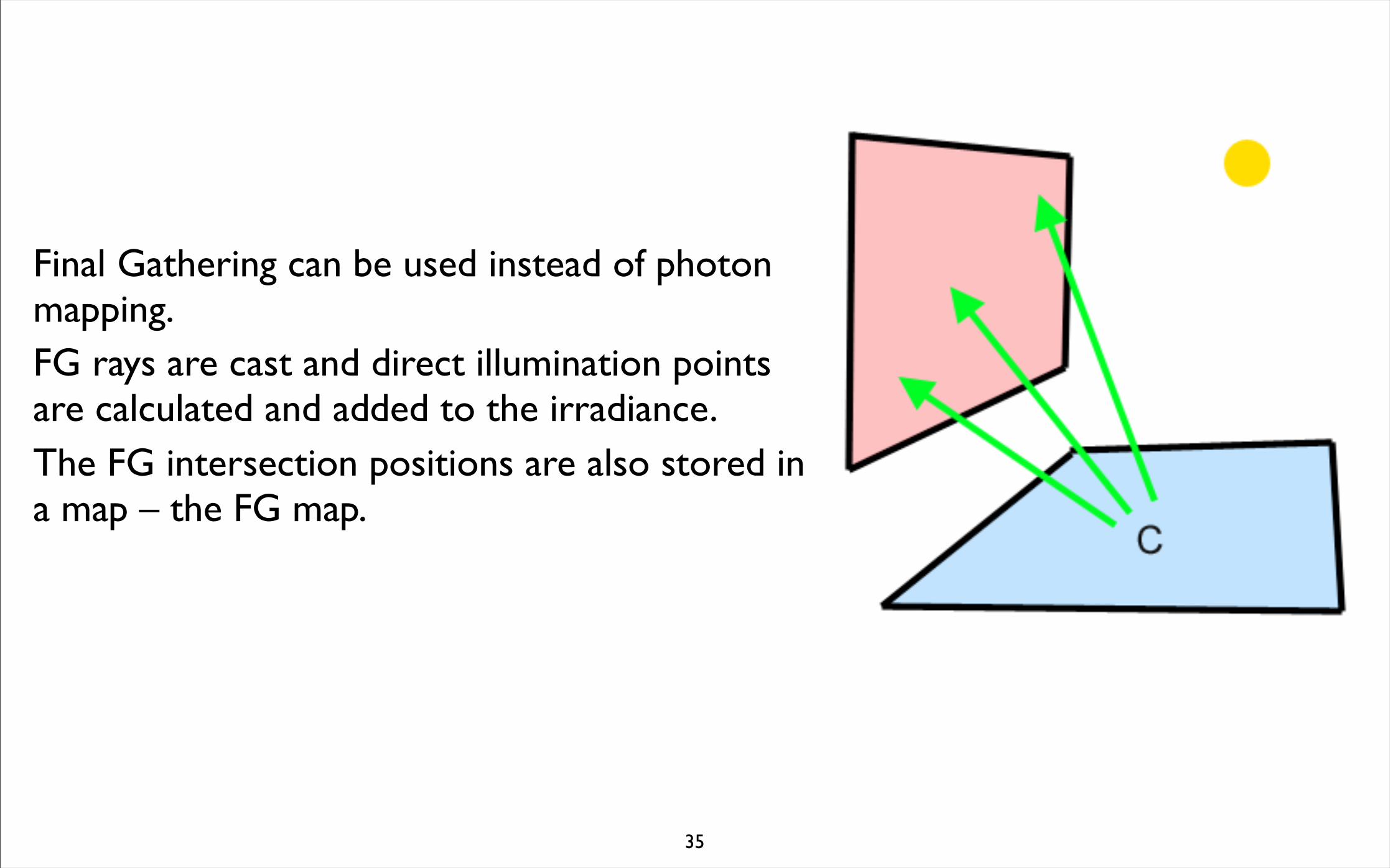
Final Gathering can be used instead of photon mapping.FG rays are cast and direct illumination points are calculated and added to the irradiance.The FG intersection positions are also stored in a map – the FG map.

36

Final Gathering vs Photon mapping

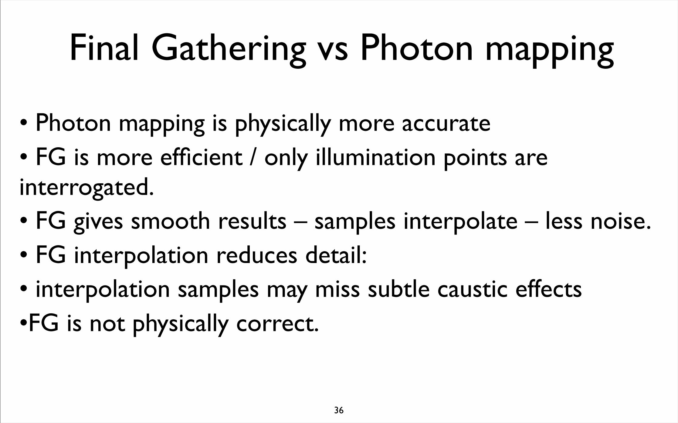
• Photon mapping is physically more accurate• FG is more efficient / only illumination points are interrogated.• FG gives smooth results – samples interpolate – less noise.• FG interpolation reduces detail:• interpolation samples may miss subtle caustic effects•FG is not physically correct.

37

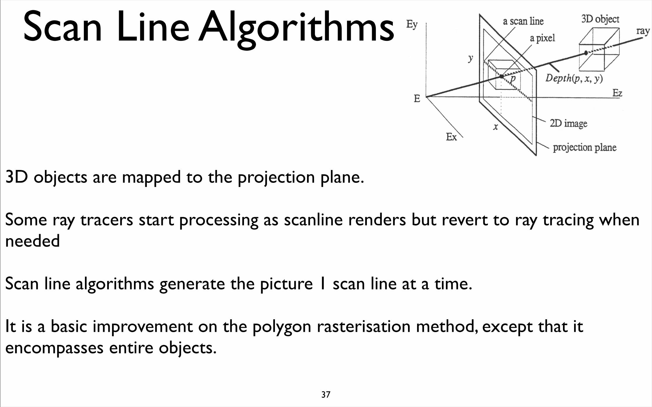
Scan Line Algorithms

3D objects are mapped to the projection plane.

Some ray tracers start processing as scanline renders but revert to ray tracing when needed

Scan line algorithms generate the picture 1 scan line at a time.

It is a basic improvement on the polygon rasterisation method, except that it encompasses entire objects.

38

That’s colour…With no direct ray tracing used in scan line renders what about…

Lighting/ShadowsReflectionsRefractions

•Most scanline algorithms use mappings to fake reflections and refractions. •These environment mapping work by rendering images that imitate the reflection seen by the surfaces and then applying these reflection and refraction maps as simple 2D textures.

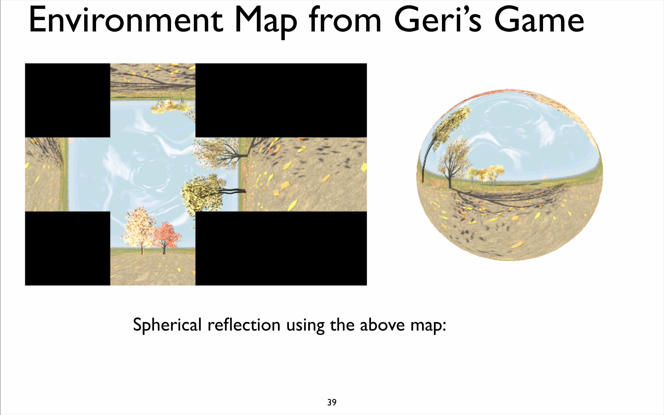
•These textures usually use simple geometric mappings – cubes and spheres.•Cubic mapping map six different views – one for each face, as in the example on the next page from Geri’s Game.

•It is worth noting that whilst animators battle against 1000’s of years of cognitive memories of human movement in producing realistic movement themselves, the human eye is much less adapt at questioning more physical properties such as reflection and refraction qualities of surfaces.

39

Environment Map from Geri’s Game

Spherical reflection using the above map:

40

Shadows

•Scan line render algorithms cannot process shadows in the same manner as ray tracers as thus use a different approach.•Question - When is an object not seen by the camera?•What approach do scan line algorithms take to implement this?•Question - When is a surface point in shadow?•What approach could scan line algorithms use based on the above?

41

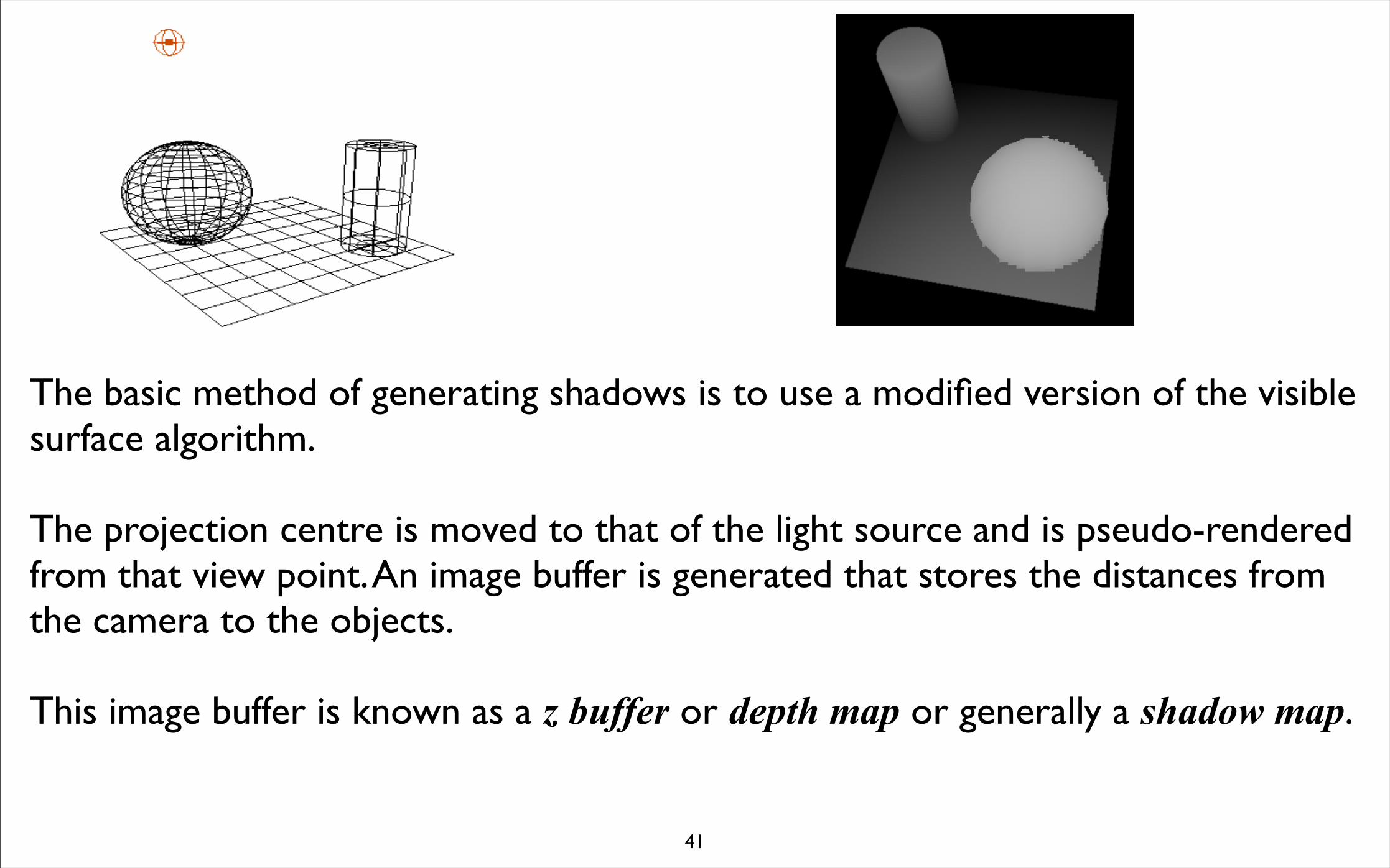
The basic method of generating shadows is to use a modified version of the visible surface algorithm.

The projection centre is moved to that of the light source and is pseudo-rendered from that view point. An image buffer is generated that stores the distances from the camera to the objects.

This image buffer is known as a z buffer or depth map or generally a shadow map.

42

When the camera projection is scan line converted, each pixel depth is converted from camera space to light space.

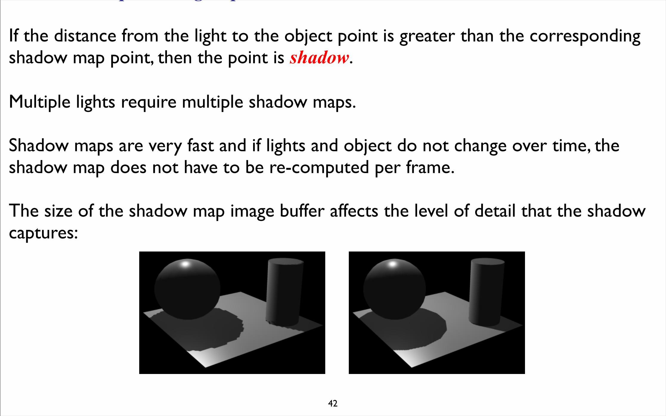
If the distance from the light to the object point is greater than the corresponding shadow map point, then the point is shadow.

Multiple lights require multiple shadow maps.

Shadow maps are very fast and if lights and object do not change over time, the shadow map does not have to be re-computed per frame.

The size of the shadow map image buffer affects the level of detail that the shadow captures:

a shadow map size of 256x256 pixels a shadow map size of 1024x1024 pixels

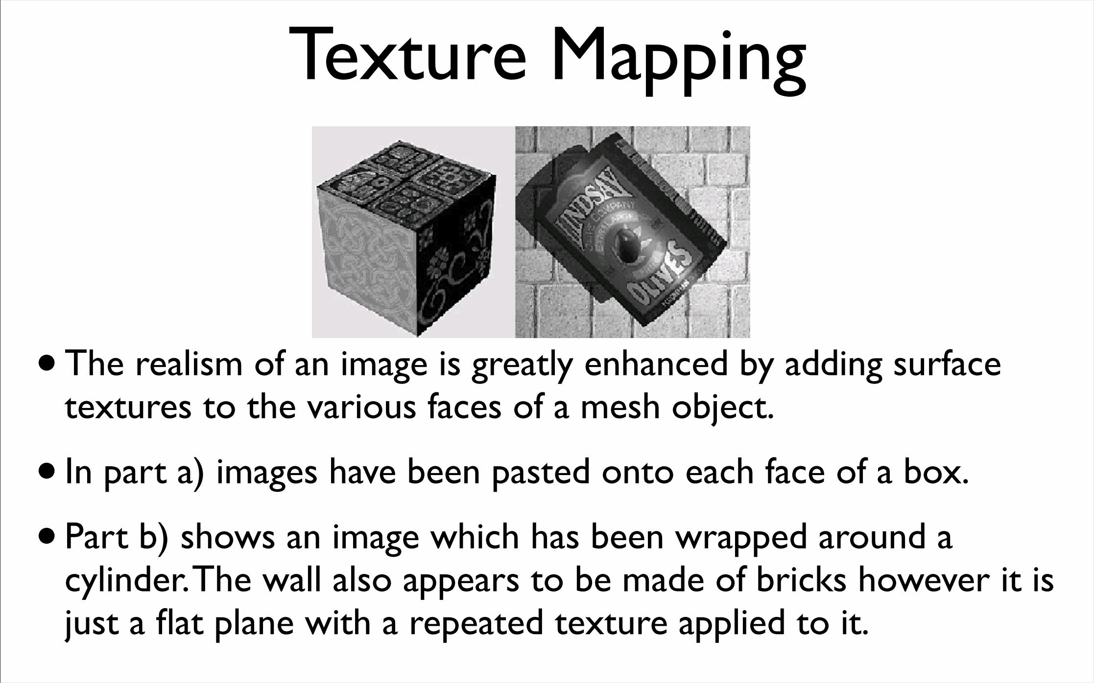
Texture Mapping

•The realism of an image is greatly enhanced by adding surface textures to the various faces of a mesh object.

• In part a) images have been pasted onto each face of a box.

• Part b) shows an image which has been wrapped around a cylinder. The wall also appears to be made of bricks however it is just a flat plane with a repeated texture applied to it.

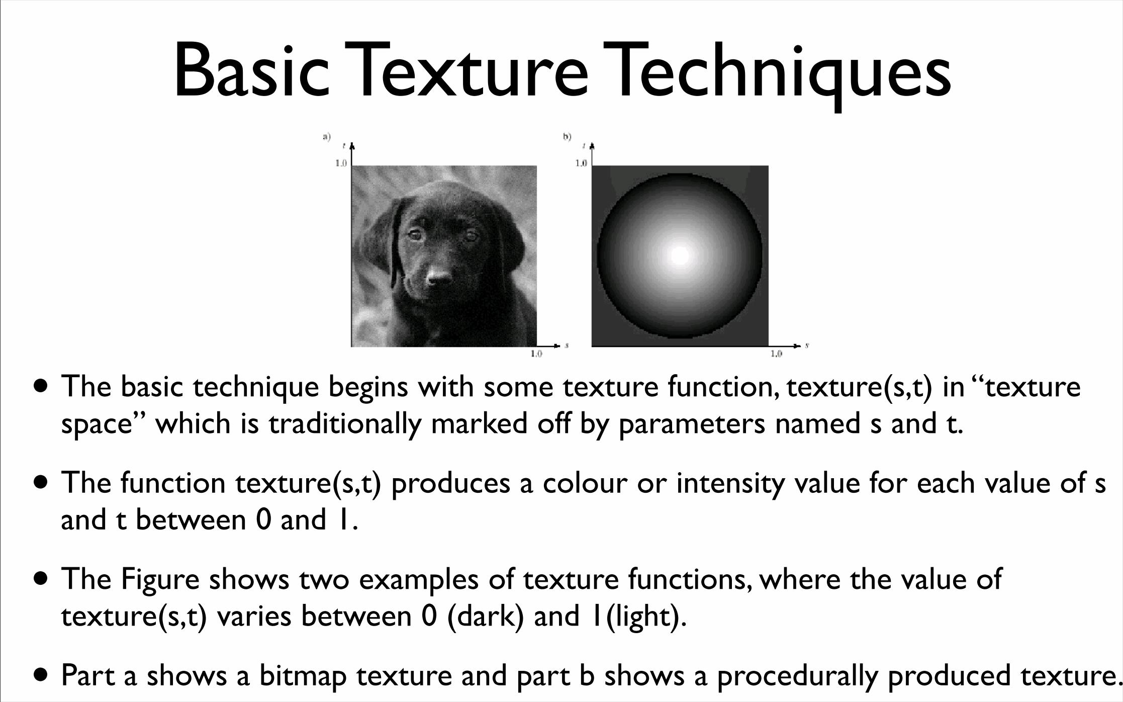
Basic Texture Techniques

• The basic technique begins with some texture function, texture(s,t) in “texture space” which is traditionally marked off by parameters named s and t.

• The function texture(s,t) produces a colour or intensity value for each value of s and t between 0 and 1.

• The Figure shows two examples of texture functions, where the value of texture(s,t) varies between 0 (dark) and 1(light).

• Part a shows a bitmap texture and part b shows a procedurally produced texture.

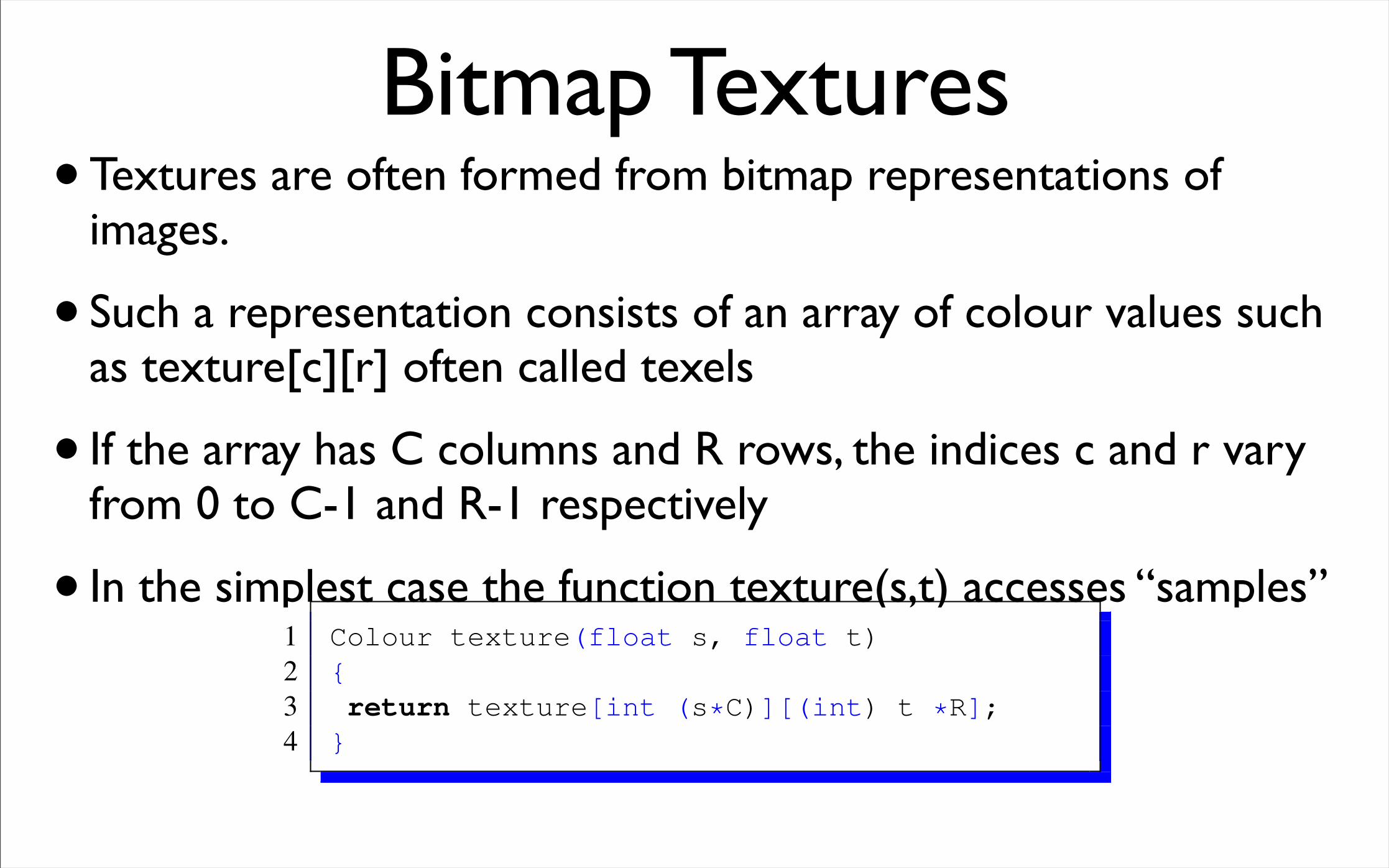
Bitmap Textures•Textures are often formed from bitmap representations of

images.

• Such a representation consists of an array of colour values such as texture[c][r] often called texels

• If the array has C columns and R rows, the indices c and r vary from 0 to C-1 and R-1 respectively

• In the simplest case the function texture(s,t) accesses “samples” 1 Colour texture(float s, float t)2 {3 return texture[int (s*C)][(int) t *R];4 }

Bitmap Textures

• In this case Colour holds an RGB triple.

• For example if R=400 and C=600, then the texture(0.261,0.783) evaluates to texture[156][313]

•Note the variation in s from 0 to 1 encompasses 600 pixels whereas the same variation in t encompasses 400 pixels.

• To avoid distortion during rendering, this texture must be mapped onto a rectangle with aspect ration 6/4.

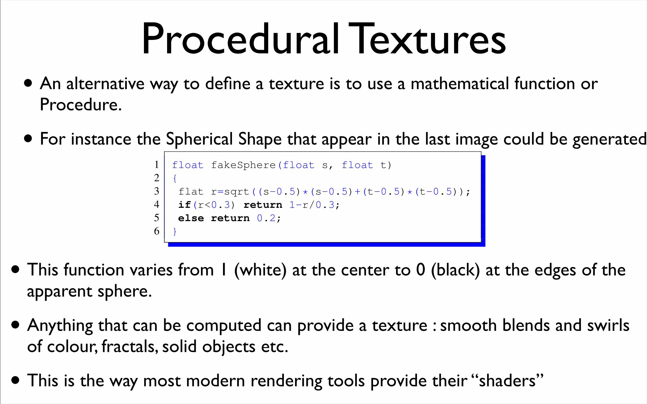
Procedural Textures• An alternative way to define a texture is to use a mathematical function or

Procedure.

• For instance the Spherical Shape that appear in the last image could be generated

• This function varies from 1 (white) at the center to 0 (black) at the edges of the apparent sphere.

• Anything that can be computed can provide a texture : smooth blends and swirls of colour, fractals, solid objects etc.

• This is the way most modern rendering tools provide their “shaders”

1 float fakeSphere(float s, float t)2 {3 flat r=sqrt((s-0.5)*(s-0.5)+(t-0.5)*(t-0.5));4 if(r<0.3) return 1-r/0.3;5 else return 0.2;6 }

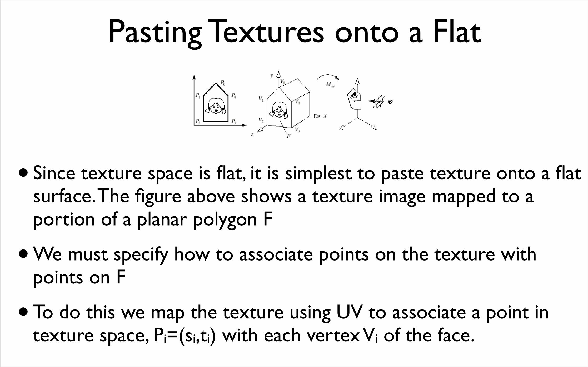
Pasting Textures onto a Flat

• Since texture space is flat, it is simplest to paste texture onto a flat surface. The figure above shows a texture image mapped to a portion of a planar polygon F

•We must specify how to associate points on the texture with points on F

• To do this we map the texture using UV to associate a point in texture space, Pi=(si,ti) with each vertex Vi of the face.

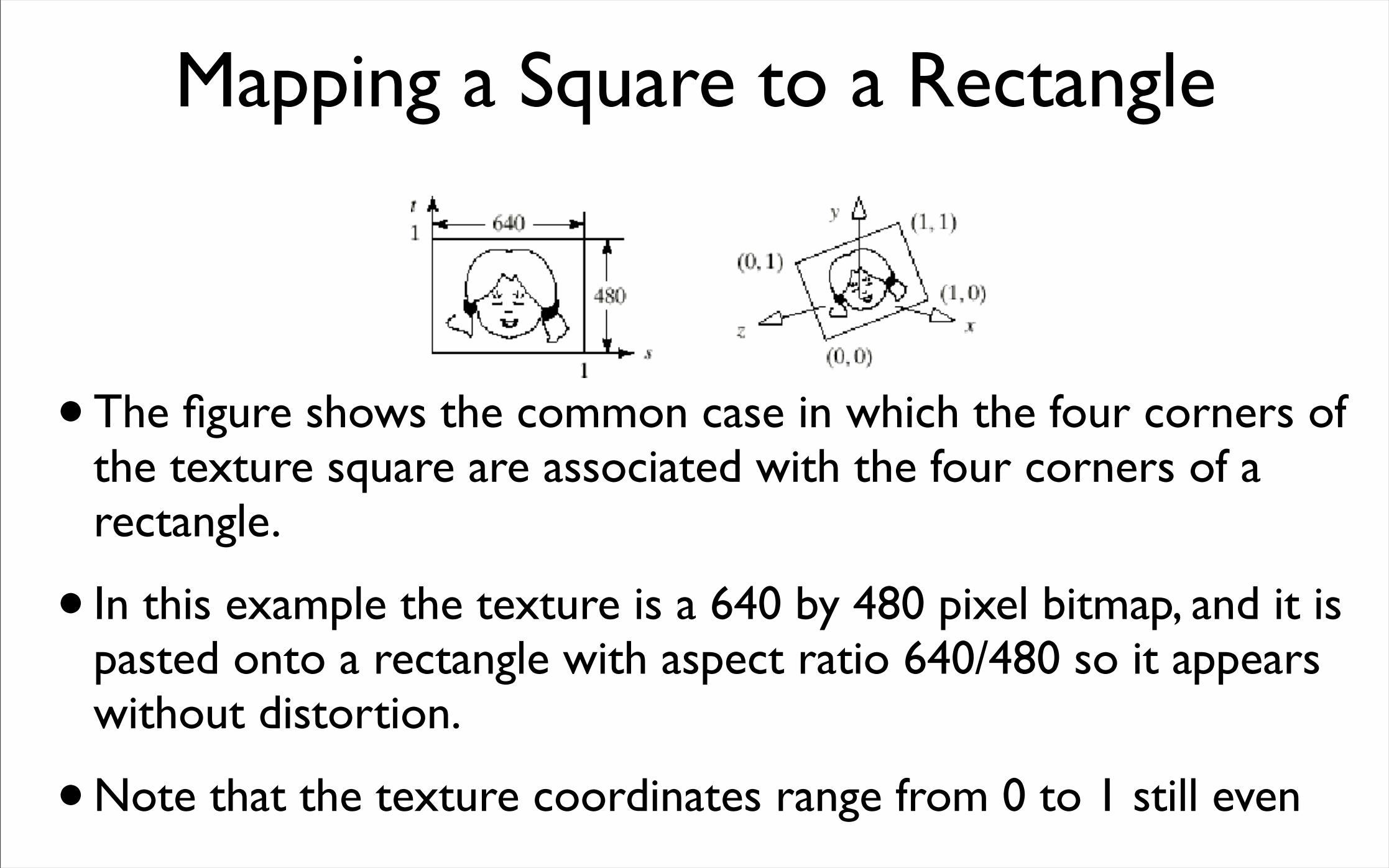
Mapping a Square to a Rectangle

•The figure shows the common case in which the four corners of the texture square are associated with the four corners of a rectangle.

• In this example the texture is a 640 by 480 pixel bitmap, and it is pasted onto a rectangle with aspect ratio 640/480 so it appears without distortion.

•Note that the texture coordinates range from 0 to 1 still even

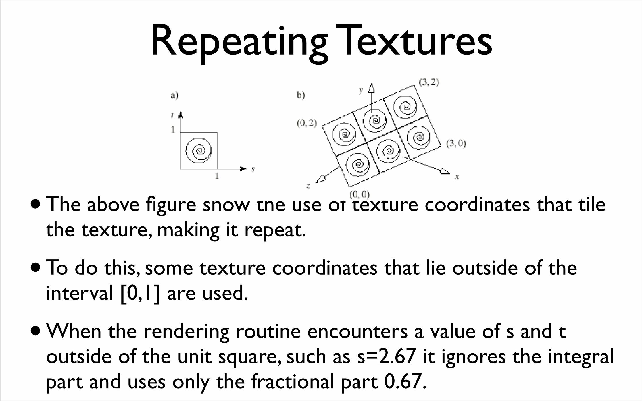
Repeating Textures

•The above figure show the use of texture coordinates that tile the texture, making it repeat.

• To do this, some texture coordinates that lie outside of the interval [0,1] are used.

•When the rendering routine encounters a value of s and t outside of the unit square, such as s=2.67 it ignores the integral part and uses only the fractional part 0.67.

Repeating Textures II

•Thus the point on a face that requires (s,t)=(2.6,3.77) is textured with texture(0.66,0.77).

• Thus, a coordinate pair (s,t) is sent down the pipeline along with each vertex of the face.

• The notion is that points inside F will be filled with texture values lying inside P by finding the internal coordinate values (s,t) through the use of interpolation.

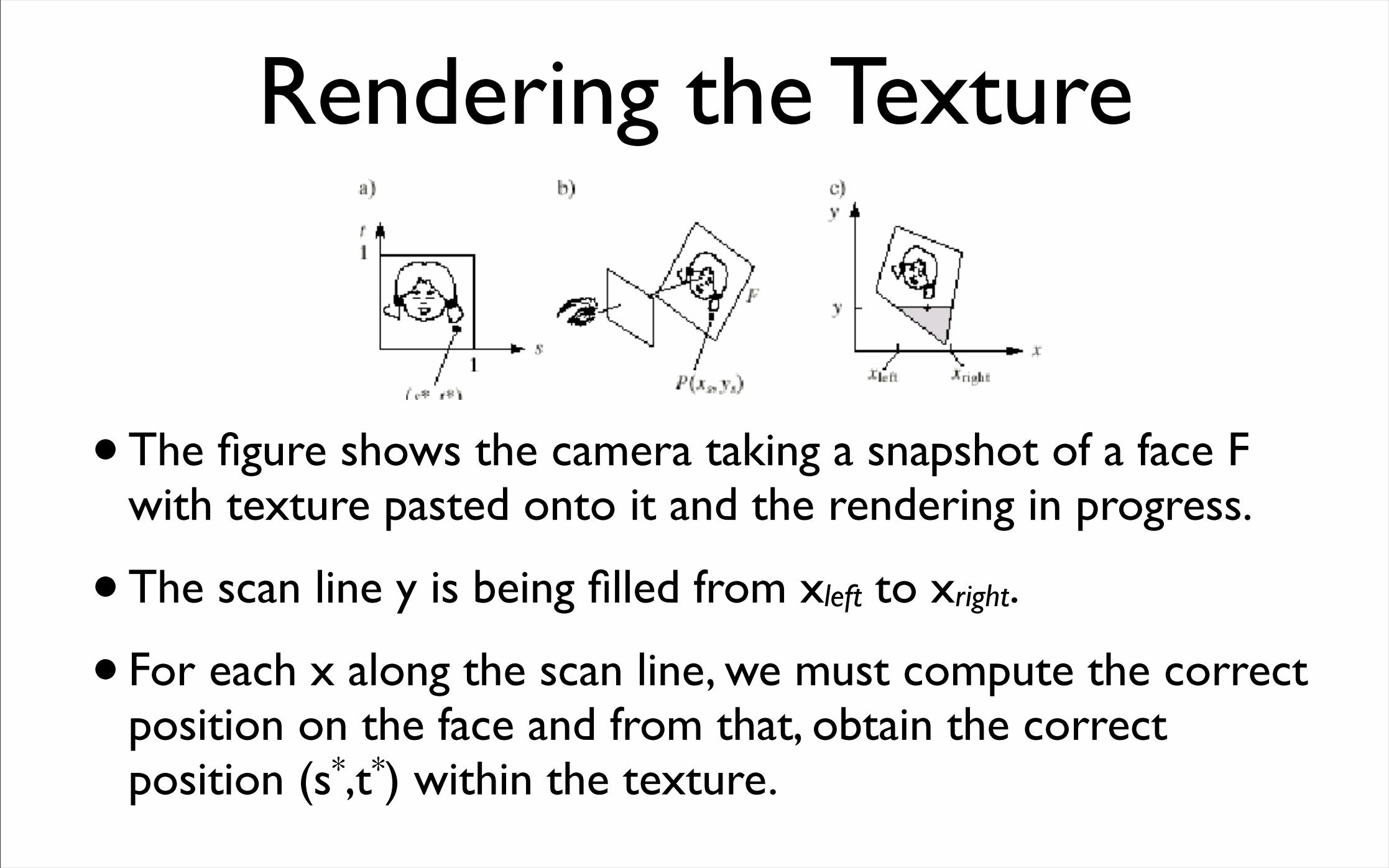
Rendering the Texture

•The figure shows the camera taking a snapshot of a face F with texture pasted onto it and the rendering in progress.

• The scan line y is being filled from xleft to xright.

• For each x along the scan line, we must compute the correct position on the face and from that, obtain the correct position (s*,t*) within the texture.

Rendering the Texture

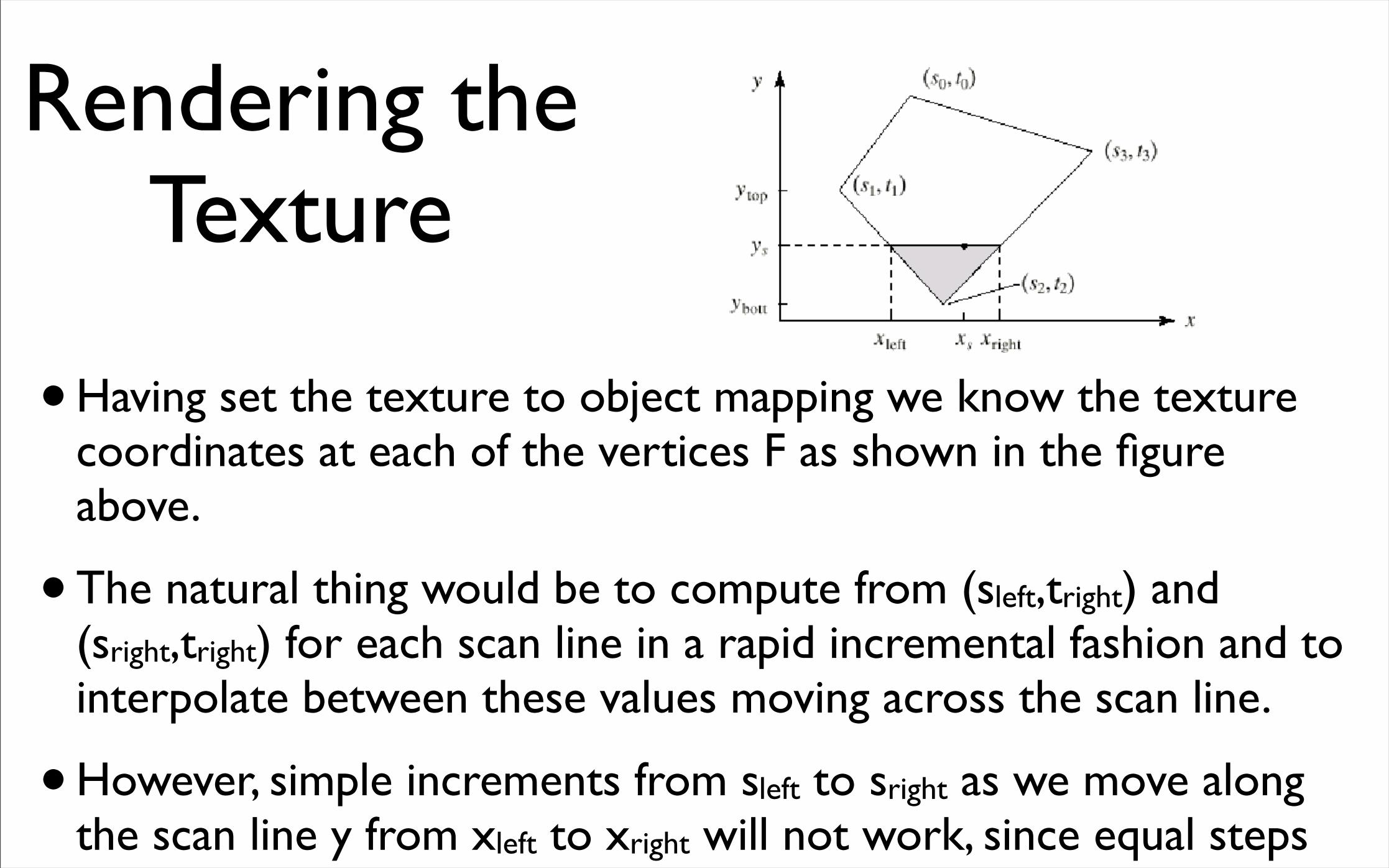
•Having set the texture to object mapping we know the texture coordinates at each of the vertices F as shown in the figure above.

• The natural thing would be to compute from (sleft,tright) and (sright,tright) for each scan line in a rapid incremental fashion and to interpolate between these values moving across the scan line.

•However, simple increments from sleft to sright as we move along the scan line y from xleft to xright will not work, since equal steps

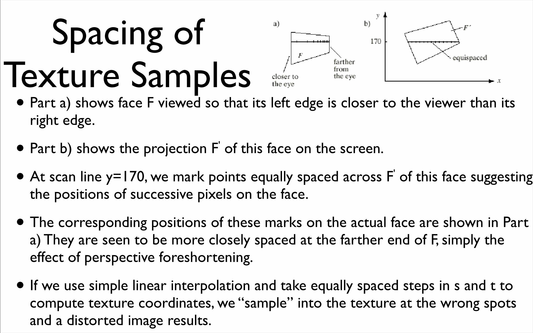
Spacing of Texture Samples• Part a) shows face F viewed so that its left edge is closer to the viewer than its

right edge.

• Part b) shows the projection F' of this face on the screen.

• At scan line y=170, we mark points equally spaced across F' of this face suggesting the positions of successive pixels on the face.

• The corresponding positions of these marks on the actual face are shown in Part a) They are seen to be more closely spaced at the farther end of F, simply the effect of perspective foreshortening.

• If we use simple linear interpolation and take equally spaced steps in s and t to compute texture coordinates, we “sample” into the texture at the wrong spots and a distorted image results.

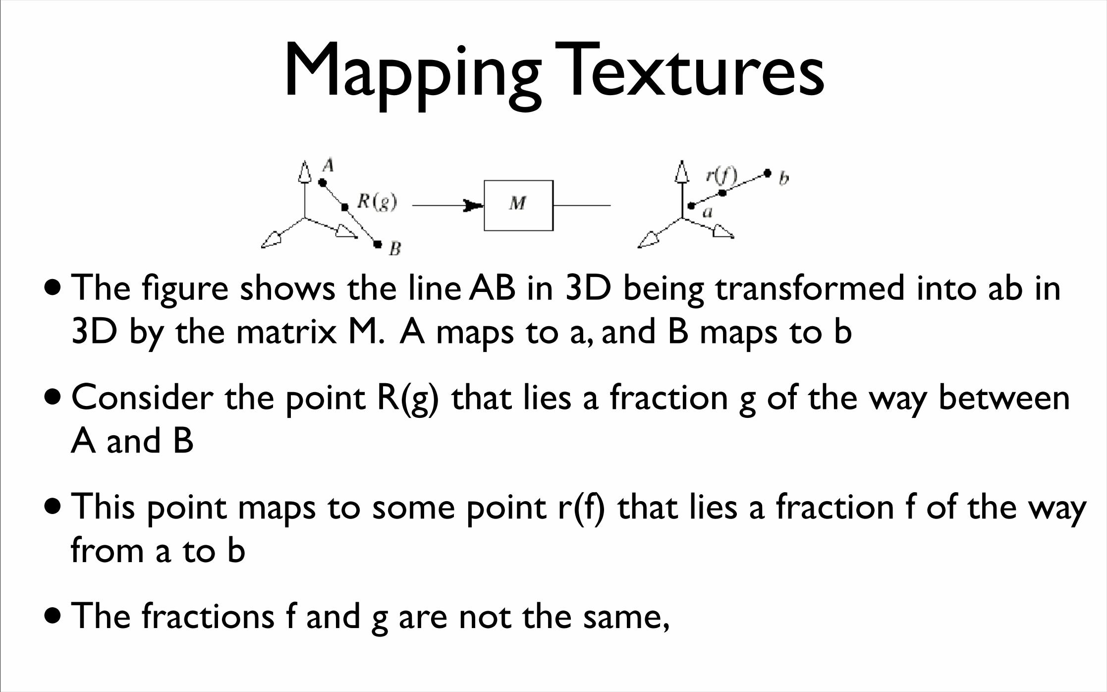
Mapping Textures

•The figure shows the line AB in 3D being transformed into ab in 3D by the matrix M. A maps to a, and B maps to b

•Consider the point R(g) that lies a fraction g of the way between A and B

•This point maps to some point r(f) that lies a fraction f of the way from a to b

• The fractions f and g are not the same,

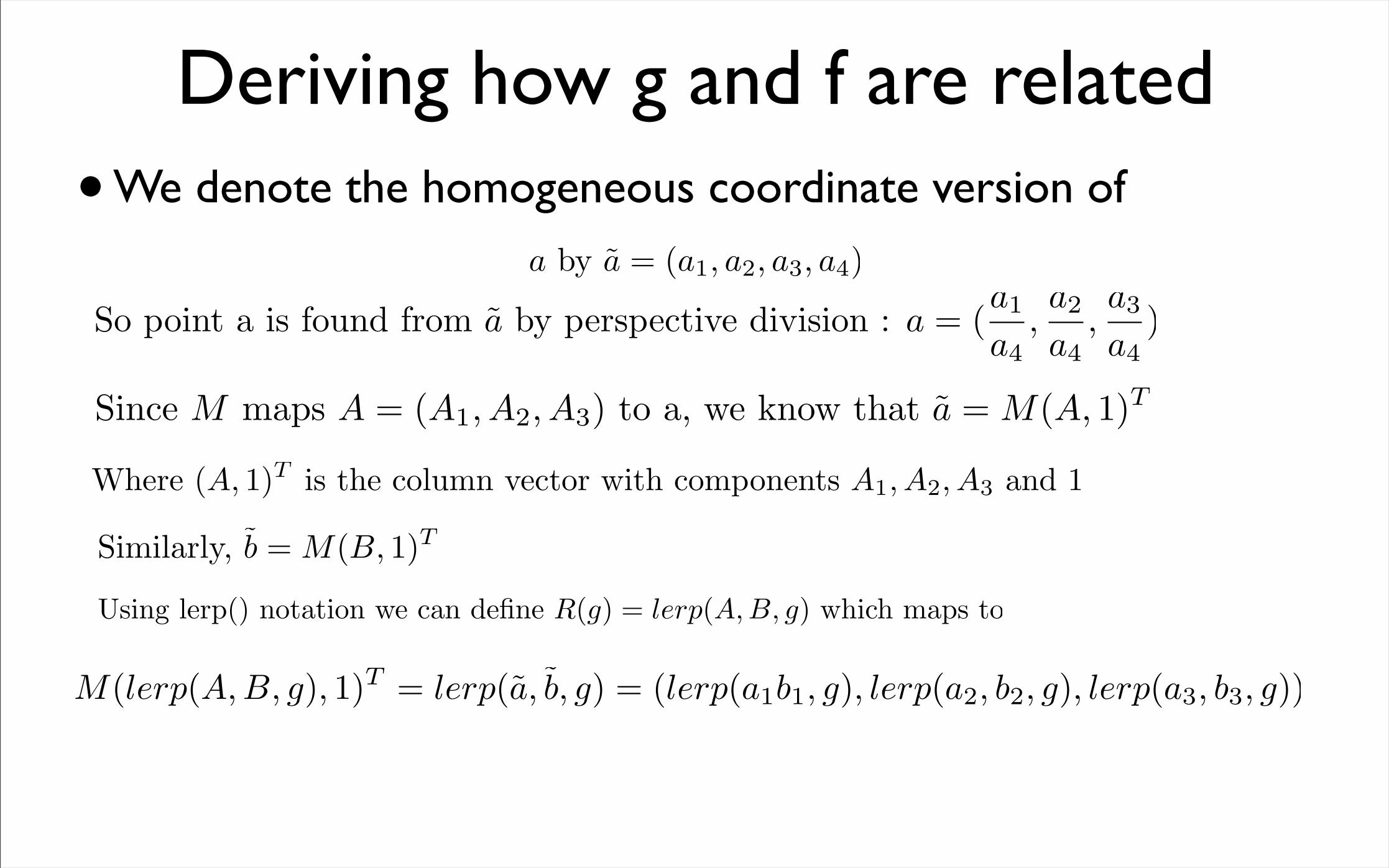
Deriving how g and f are related•We denote the homogeneous coordinate version of

a by a = (a1, a2, a3, a4)

So point a is found from a by perspective division : a = (a1

a4,a2

a4,a3

a4)

Since M maps A = (A1, A2, A3) to a, we know that a = M(A, 1)T

Where (A, 1)T is the column vector with components A1, A2, A3 and 1

Similarly, b = M(B, 1)T

Using lerp() notation we can define R(g) = lerp(A, B, g) which maps to

M(lerp(A, B, g), 1)T = lerp(a, b, g) = (lerp(a1b1, g), lerp(a2, b2, g), lerp(a3, b3, g))

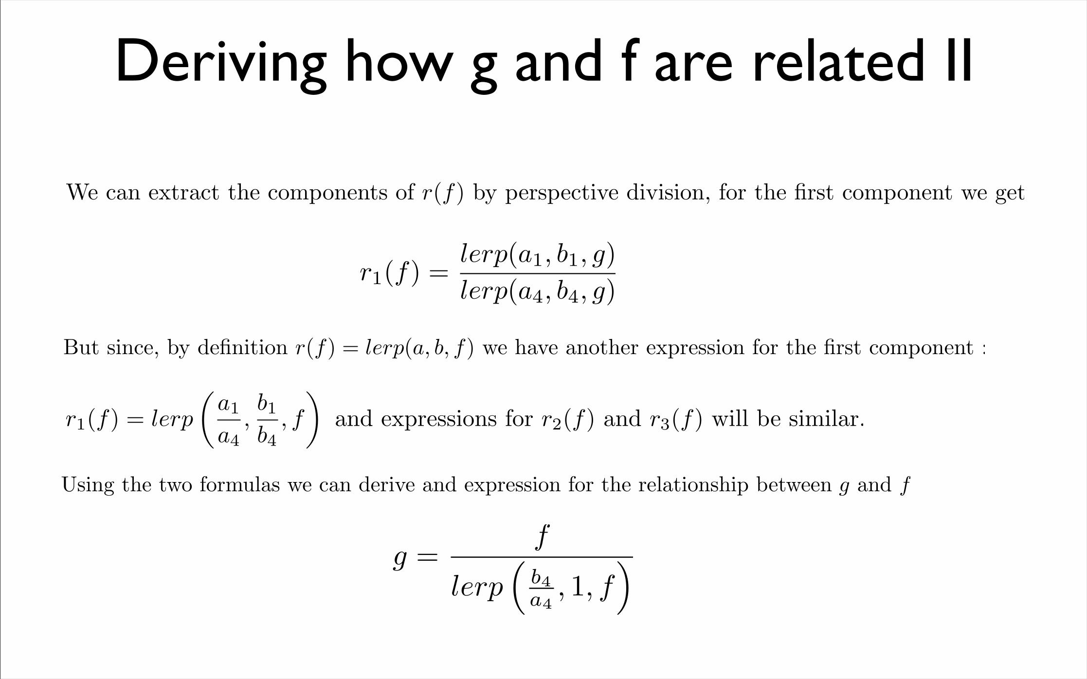
Deriving how g and f are related II

We can extract the components of r(f) by perspective division, for the first component we get

r1(f) =lerp(a1, b1, g)lerp(a4, b4, g)

But since, by definition r(f) = lerp(a, b, f) we have another expression for the first component :

r1(f) = lerp

(a1

a4,b1

b4, f

)and expressions for r2(f) and r3(f) will be similar.

Using the two formulas we can derive and expression for the relationship between g and f

g =f

lerp(

b4a4

, 1, f)

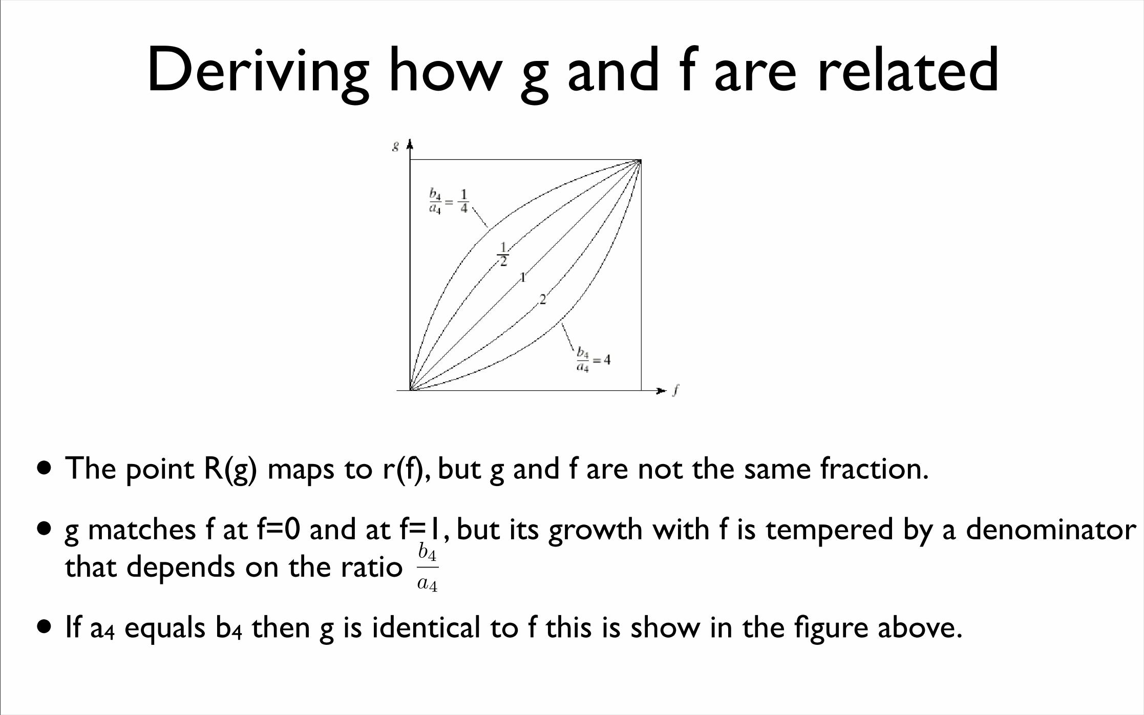
Deriving how g and f are related

• The point R(g) maps to r(f), but g and f are not the same fraction.

• g matches f at f=0 and at f=1, but its growth with f is tempered by a denominator that depends on the ratio

• If a4 equals b4 then g is identical to f this is show in the figure above.

b4

a4

Deriving how g and f are related

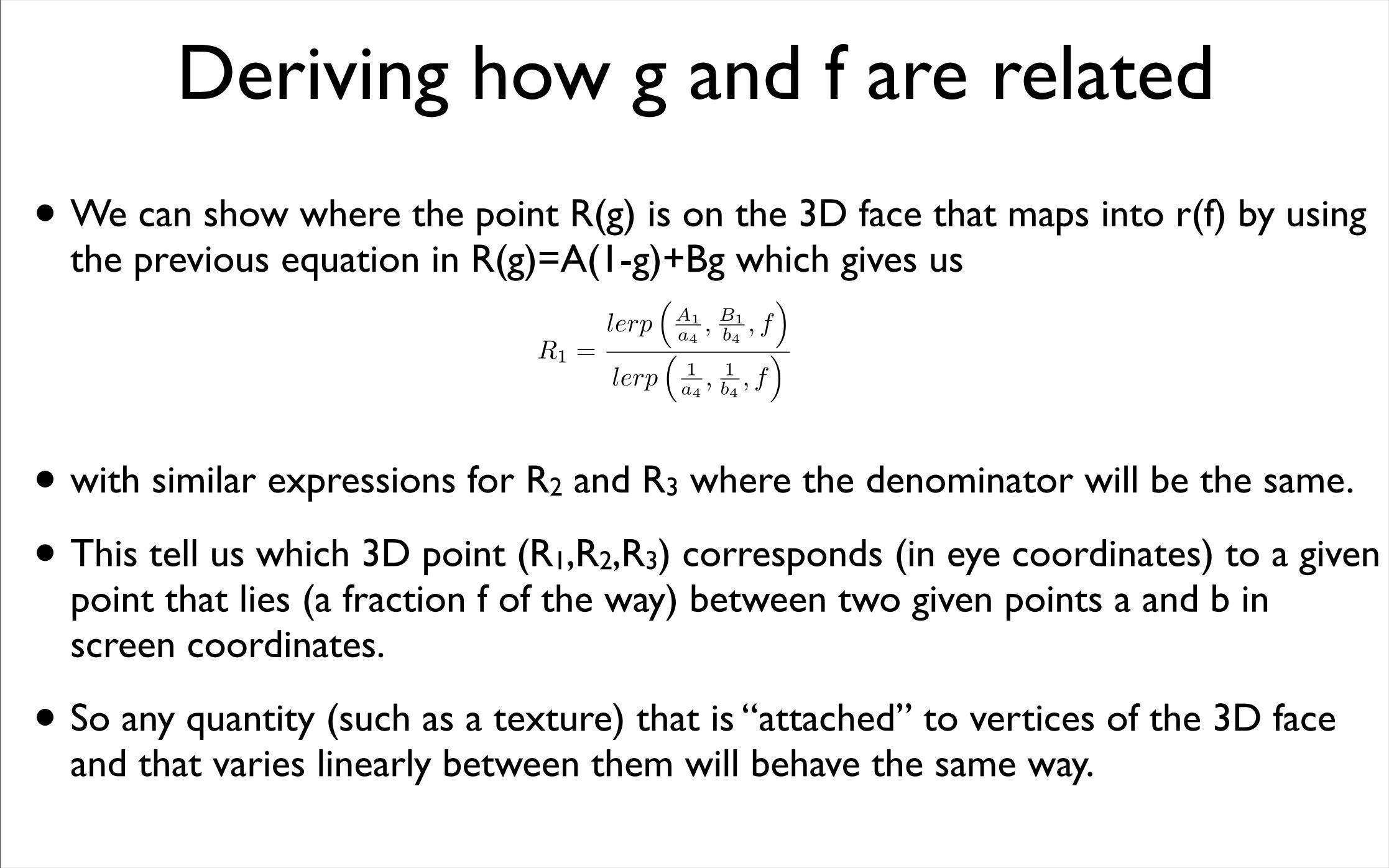
• We can show where the point R(g) is on the 3D face that maps into r(f) by using the previous equation in R(g)=A(1-g)+Bg which gives us

• with similar expressions for R2 and R3 where the denominator will be the same.

• This tell us which 3D point (R1,R2,R3) corresponds (in eye coordinates) to a given point that lies (a fraction f of the way) between two given points a and b in screen coordinates.

• So any quantity (such as a texture) that is “attached” to vertices of the 3D face and that varies linearly between them will behave the same way.

R1 =lerp

(A1a4

, B1b4

, f)

lerp(

1a4

, 1b4

, f)

Rendering Images

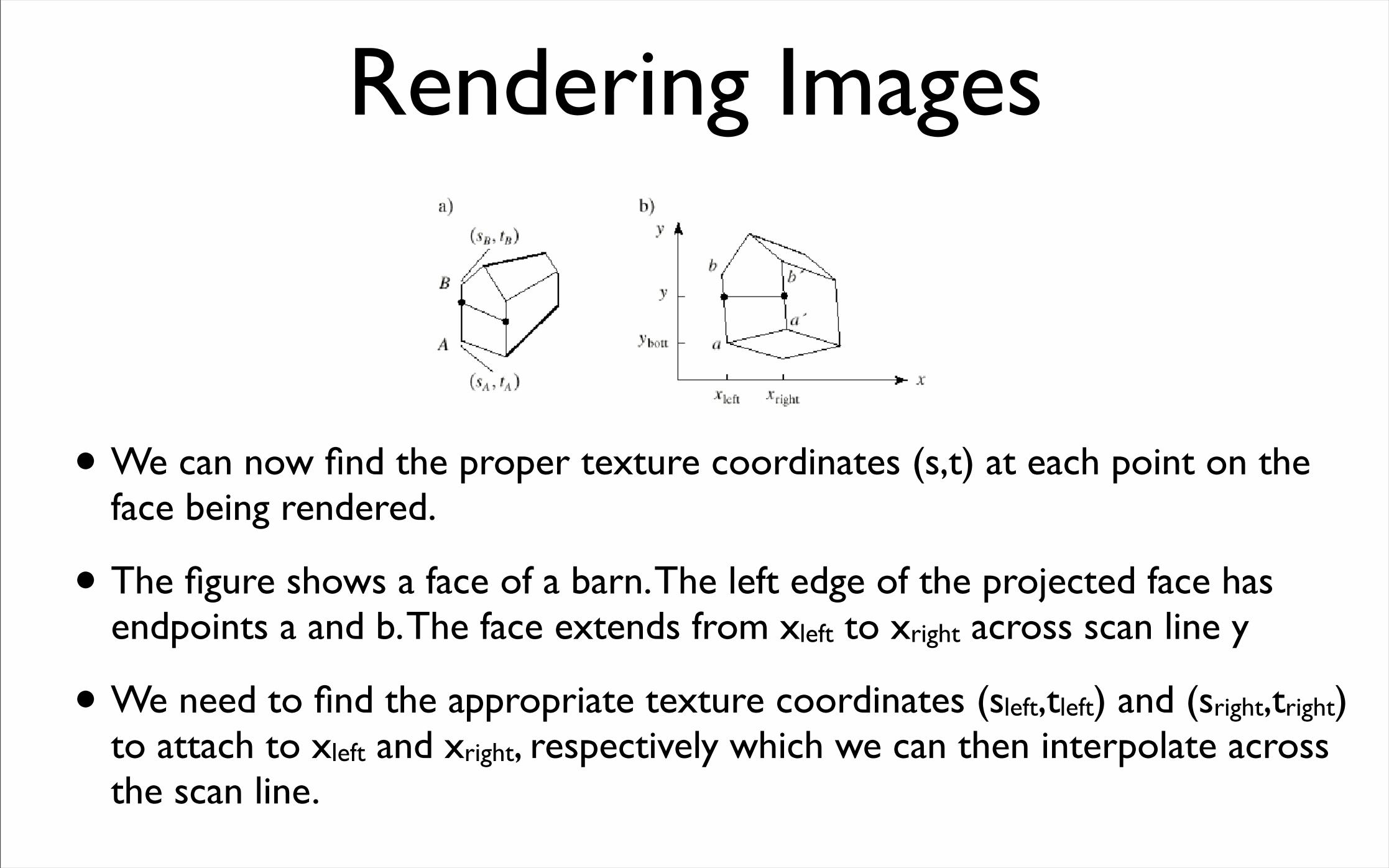
• We can now find the proper texture coordinates (s,t) at each point on the face being rendered.

• The figure shows a face of a barn. The left edge of the projected face has endpoints a and b. The face extends from xleft to xright across scan line y

• We need to find the appropriate texture coordinates (sleft,tleft) and (sright,tright) to attach to xleft and xright, respectively which we can then interpolate across the scan line.

Rendering Images Incrementally II

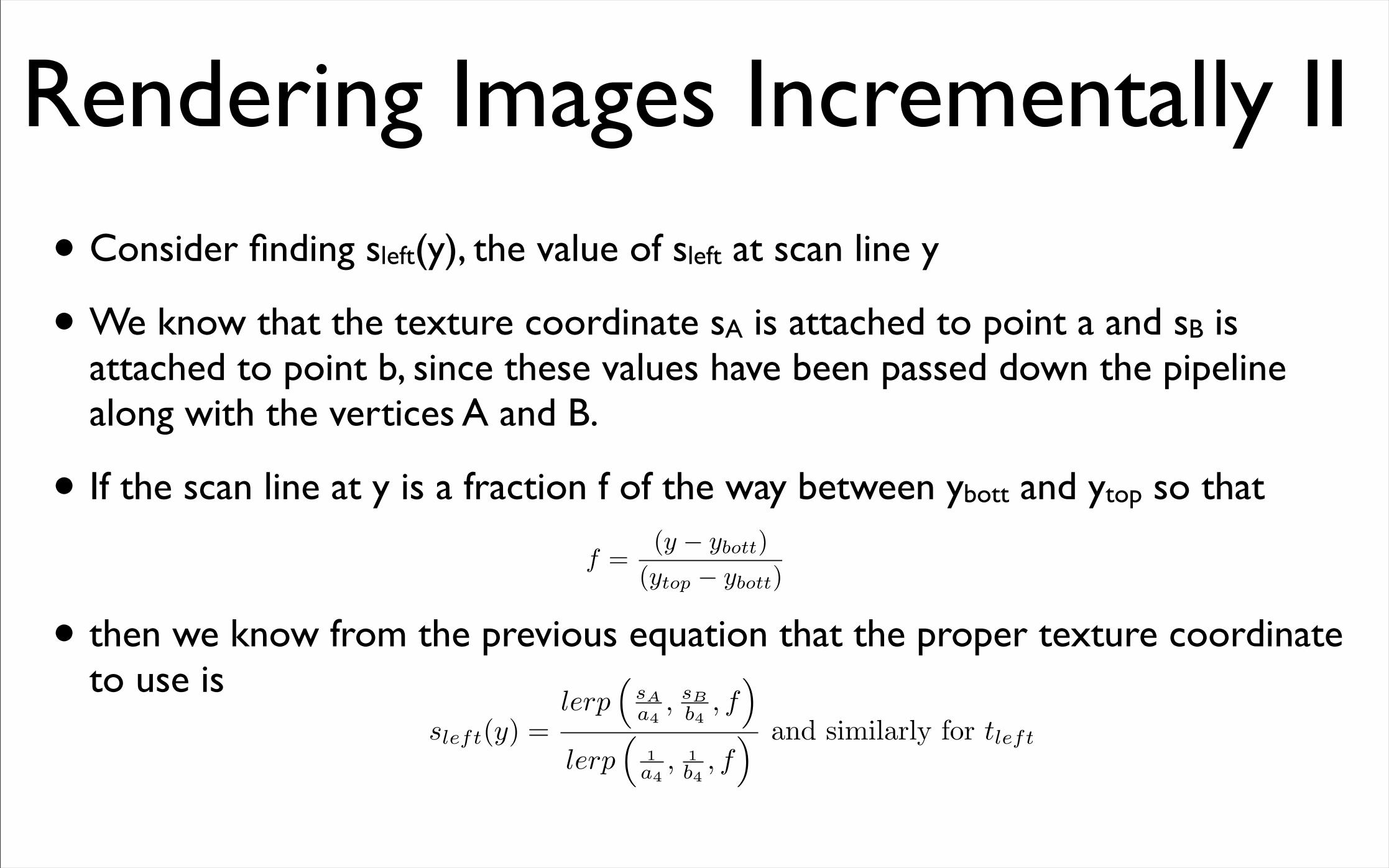
• Consider finding sleft(y), the value of sleft at scan line y

• We know that the texture coordinate sA is attached to point a and sB is attached to point b, since these values have been passed down the pipeline along with the vertices A and B.

• If the scan line at y is a fraction f of the way between ybott and ytop so that

• then we know from the previous equation that the proper texture coordinate to use is

f =(y − ybott)

(ytop − ybott)

sleft(y) =lerp

(sAa4

, sBb4

, f)

lerp(

1a4

, 1b4

, f) and similarly for tleft

Rendering Images Incrementally III•Notice that sleft and tleft have the same denominator : a linear

interpolation between the values 1/a4 and 1/b4

• The numerator terms are linear interpolation of texture coordinates that have been divided by a4 and b4. This technique is called “hyperbolic interpolation”

•Once (sleft,tleft) and (sright,tright) have been found, the scan line can be filled.

• For each x from xleft to xright, the values s and t are found by hyperbolic interpolation.

63

References• Computer Graphics Foley van Dam et al

• Realistic Image Synthesis Using Photon Mapping Henrik Wann Jensen

• Computer Graphics with OpenGL F.S. Hill

• Production Rendering Ian Stephenson (Ed.)

• http://en.wikipedia.org/wiki/Raytracing

• http://en.wikipedia.org/wiki/Radiosity

• http://freespace.virgin.net/hugo.elias/radiosity/radiosity.htm

• http://en.wikipedia.org/wiki/Global_illumination