Embed Size (px)
Citation preview
Real-time CNC interpolatoralgorithms for motion control
Rida T. Farouki
Department of Mechanical & Aeronautical Engineering,University of California, Davis
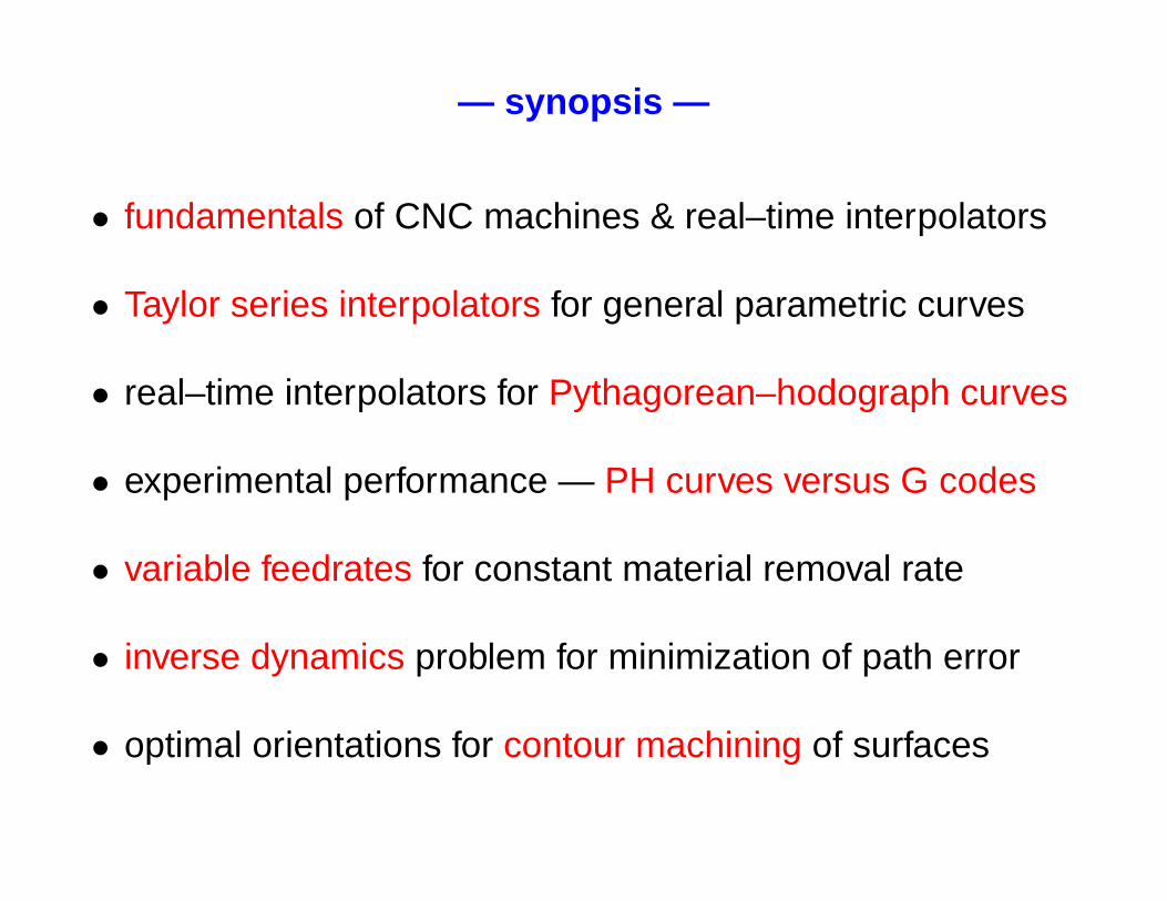
— synopsis —
• fundamentals of CNC machines & real–time interpolators
• Taylor series interpolators for general parametric curves
• real–time interpolators for Pythagorean–hodograph curves
• experimental performance — PH curves versus G codes
• variable feedrates for constant material removal rate
• inverse dynamics problem for minimization of path error
• optimal orientations for contour machining of surfaces
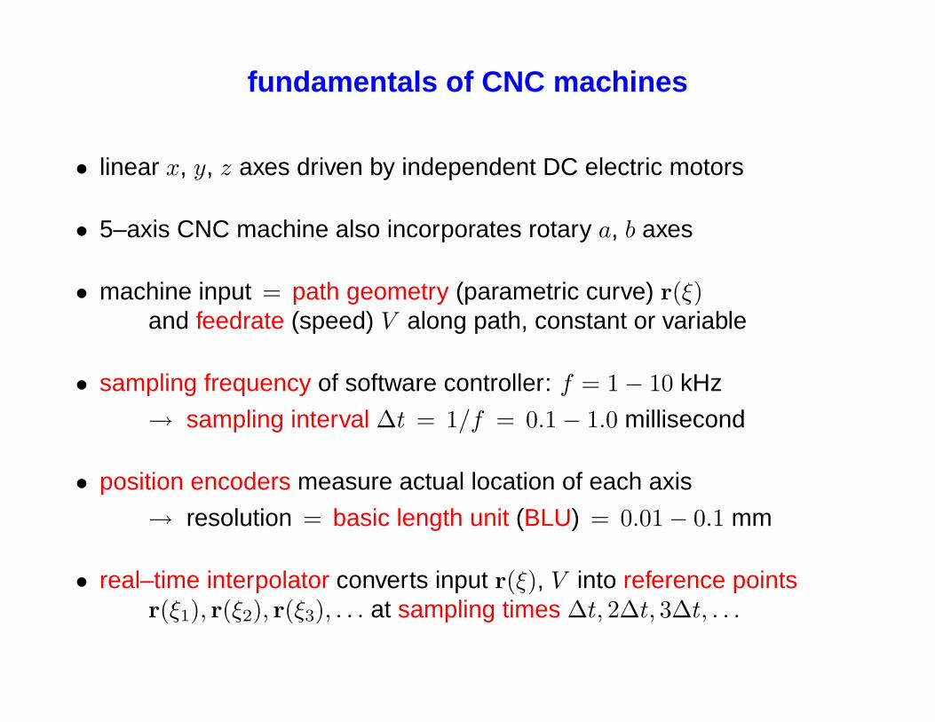
fundamentals of CNC machines
• linear x, y, z axes driven by independent DC electric motors
• 5–axis CNC machine also incorporates rotary a, b axes
• machine input = path geometry (parametric curve) r(ξ)and feedrate (speed) V along path, constant or variable
• sampling frequency of software controller: f = 1− 10 kHz
→ sampling interval ∆t = 1/f = 0.1− 1.0 millisecond
• position encoders measure actual location of each axis
→ resolution = basic length unit (BLU) = 0.01− 0.1 mm
• real–time interpolator converts input r(ξ), V into reference pointsr(ξ1), r(ξ2), r(ξ3), . . . at sampling times ∆t, 2∆t, 3∆t, . . .
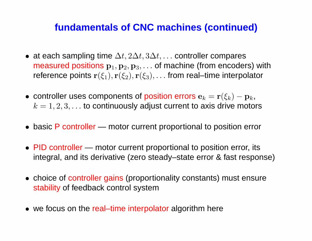
fundamentals of CNC machines (continued)
• at each sampling time ∆t, 2∆t, 3∆t, . . . controller comparesmeasured positions p1,p2,p3, . . . of machine (from encoders) withreference points r(ξ1), r(ξ2), r(ξ3), . . . from real–time interpolator
• controller uses components of position errors ek = r(ξk)− pk,k = 1, 2, 3, . . . to continuously adjust current to axis drive motors
• basic P controller — motor current proportional to position error
• PID controller — motor current proportional to position error, itsintegral, and its derivative (zero steady–state error & fast response)
• choice of controller gains (proportionality constants) must ensurestability of feedback control system
• we focus on the real–time interpolator algorithm here
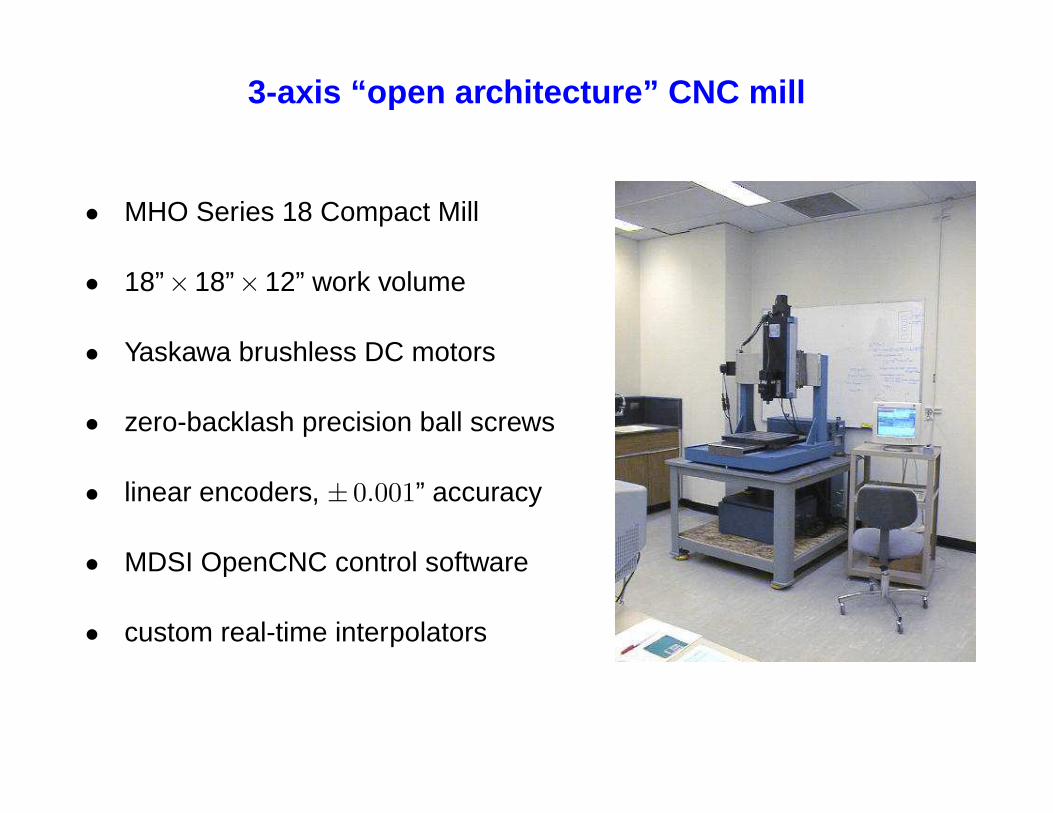
3-axis “open architecture” CNC mill
• MHO Series 18 Compact Mill
• 18”×18”×12” work volume
• Yaskawa brushless DC motors
• zero-backlash precision ball screws
• linear encoders, ± 0.001” accuracy
• MDSI OpenCNC control software
• custom real-time interpolators
��������������������������������������������������������������������������������������������������������������������������������������������������������������������������������������������������������������������������������������������������������������������������������������������������������������������������������������������������������������������������������������������������������������������������������������������������������������������������������������������������������������������
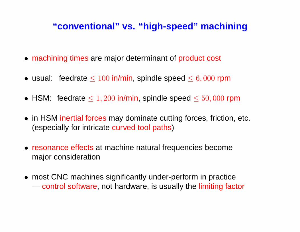
“conventional” vs. “high-speed” machining
• machining times are major determinant of product cost
• usual: feedrate ≤ 100 in/min, spindle speed ≤ 6, 000 rpm
• HSM: feedrate ≤ 1, 200 in/min, spindle speed ≤ 50, 000 rpm
• in HSM inertial forces may dominate cutting forces, friction, etc.(especially for intricate curved tool paths)
• resonance effects at machine natural frequencies becomemajor consideration
• most CNC machines significantly under-perform in practice— control software, not hardware, is usually the limiting factor
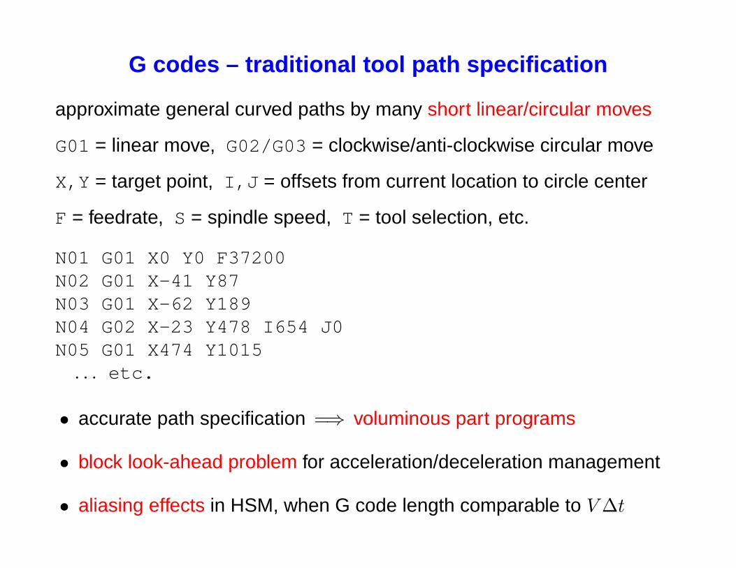
G codes – traditional tool path specification
approximate general curved paths by many short linear/circular moves
G01 = linear move, G02/G03 = clockwise/anti-clockwise circular move
X,Y = target point, I,J = offsets from current location to circle center
F = feedrate, S = spindle speed, T = tool selection, etc.
N01 G01 X0 Y0 F37200N02 G01 X-41 Y87N03 G01 X-62 Y189N04 G02 X-23 Y478 I654 J0N05 G01 X474 Y1015. . . etc.
• accurate path specification =⇒ voluminous part programs
• block look-ahead problem for acceleration/deceleration management
• aliasing effects in HSM, when G code length comparable to V∆t
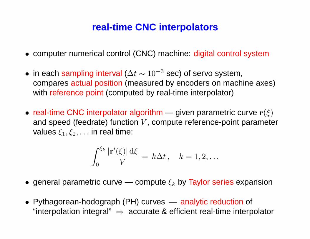
real-time CNC interpolators
• computer numerical control (CNC) machine: digital control system
• in each sampling interval (∆t ∼ 10−3 sec) of servo system,compares actual position (measured by encoders on machine axes)with reference point (computed by real-time interpolator)
• real-time CNC interpolator algorithm — given parametric curve r(ξ)and speed (feedrate) function V , compute reference-point parametervalues ξ1, ξ2, . . . in real time:∫ ξk
0
|r′(ξ)|dξV
= k∆t , k = 1, 2, . . .
• general parametric curve — compute ξk by Taylor series expansion
• Pythagorean-hodograph (PH) curves — analytic reduction of“interpolation integral” ⇒ accurate & efficient real-time interpolator
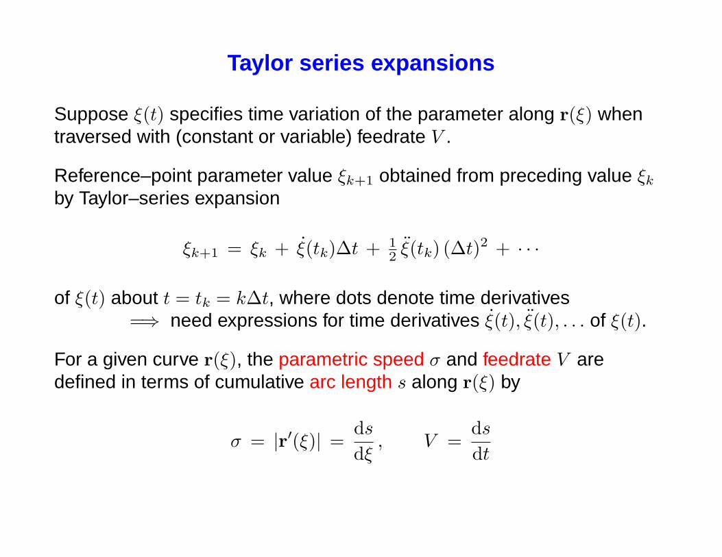
Taylor series expansions
Suppose ξ(t) specifies time variation of the parameter along r(ξ) whentraversed with (constant or variable) feedrate V .
Reference–point parameter value ξk+1 obtained from preceding value ξkby Taylor–series expansion
ξk+1 = ξk + ξ(tk)∆t + 12 ξ(tk) (∆t)2 + · · ·
of ξ(t) about t = tk = k∆t, where dots denote time derivatives=⇒ need expressions for time derivatives ξ(t), ξ(t), . . . of ξ(t).
For a given curve r(ξ), the parametric speed σ and feedrate V aredefined in terms of cumulative arc length s along r(ξ) by
σ = |r′(ξ)| =dsdξ, V =
dsdt
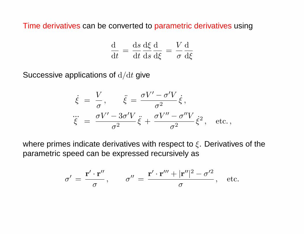
Time derivatives can be converted to parametric derivatives using
ddt
=dsdt
dξds
ddξ
=V
σ
ddξ
Successive applications of d/dt give
ξ =V
σ, ξ =
σV ′ − σ′V
σ2ξ ,
...ξ =
σV ′ − 3σ′Vσ2
ξ +σV ′′ − σ′′V
σ2ξ2 , etc. ,
where primes indicate derivatives with respect to ξ. Derivatives of theparametric speed can be expressed recursively as
σ′ =r′ · r′′
σ, σ′′ =
r′ · r′′′ + |r′′|2 − σ′2
σ, etc.
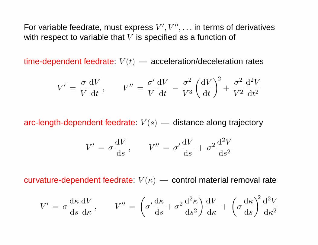
For variable feedrate, must express V ′, V ′′, . . . in terms of derivativeswith respect to variable that V is specified as a function of
time-dependent feedrate: V (t) — acceleration/deceleration rates
V ′ =σ
V
dVdt
, V ′′ =σ′
V
dVdt
− σ2
V 3
(dVdt
)2
+σ2
V 2
d2V
dt2
arc-length-dependent feedrate: V (s) — distance along trajectory
V ′ = σdVds
, V ′′ = σ′dVds
+ σ2 d2V
ds2
curvature-dependent feedrate: V (κ) — control material removal rate
V ′ = σdκds
dVdκ
, V ′′ =(σ′
dκds
+ σ2 d2κ
ds2
)dVdκ
+(σ
dκds
)2 d2V
dκ2
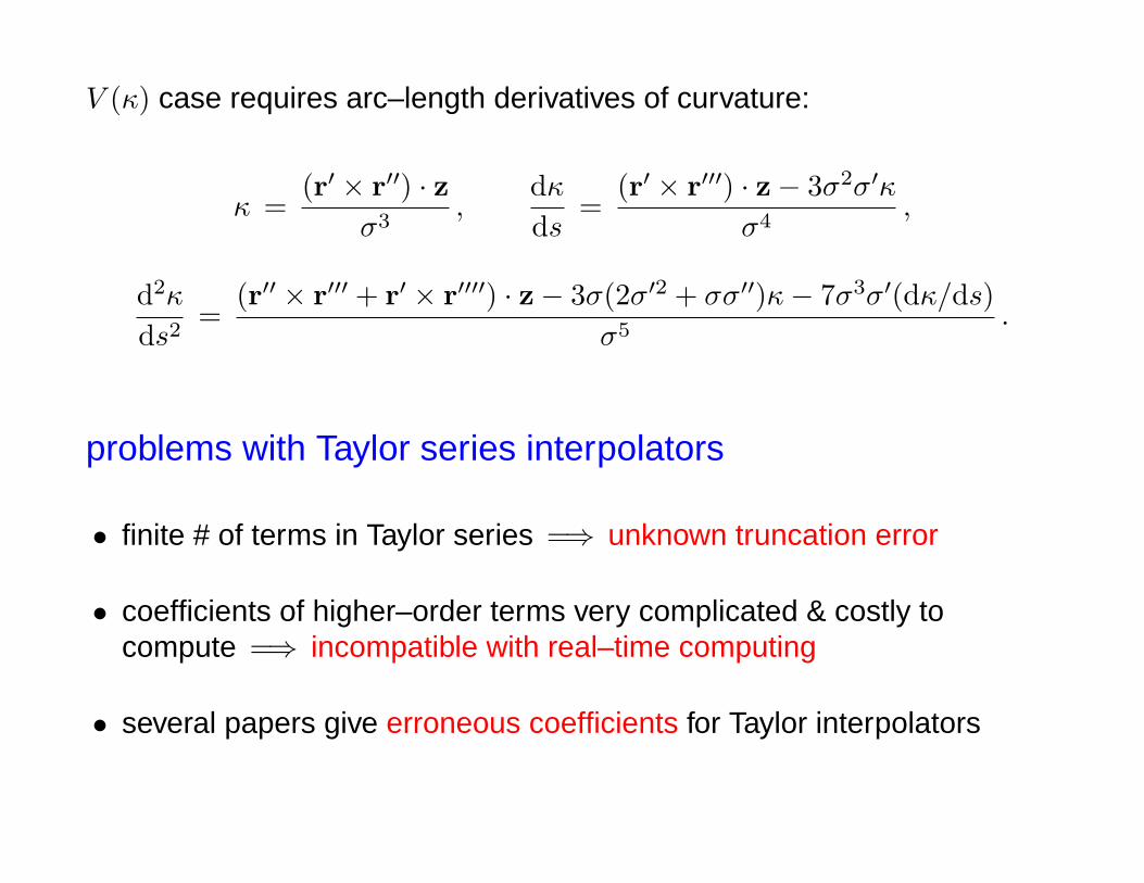
V (κ) case requires arc–length derivatives of curvature:
κ =(r′ × r′′) · z
σ3,
dκds
=(r′ × r′′′) · z− 3σ2σ′κ
σ4,
d2κ
ds2=
(r′′ × r′′′ + r′ × r′′′′) · z− 3σ(2σ′2 + σσ′′)κ− 7σ3σ′(dκ/ds)σ5
.
problems with Taylor series interpolators
• finite # of terms in Taylor series =⇒ unknown truncation error
• coefficients of higher–order terms very complicated & costly tocompute =⇒ incompatible with real–time computing
• several papers give erroneous coefficients for Taylor interpolators
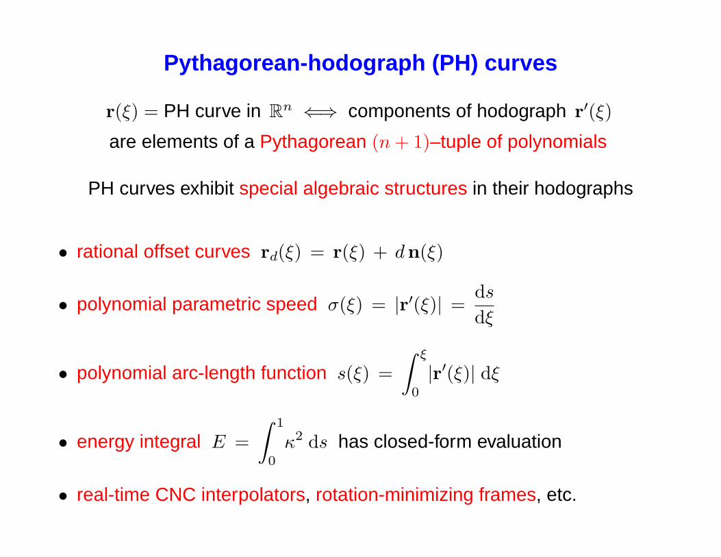
Pythagorean-hodograph (PH) curves
r(ξ) = PH curve in Rn ⇐⇒ components of hodograph r′(ξ)
are elements of a Pythagorean (n+ 1)–tuple of polynomials
PH curves exhibit special algebraic structures in their hodographs
• rational offset curves rd(ξ) = r(ξ) + dn(ξ)
• polynomial parametric speed σ(ξ) = |r′(ξ)| =dsdξ
• polynomial arc-length function s(ξ) =∫ ξ
0
|r′(ξ)| dξ
• energy integral E =∫ 1
0
κ2 ds has closed-form evaluation
• real-time CNC interpolators, rotation-minimizing frames, etc.
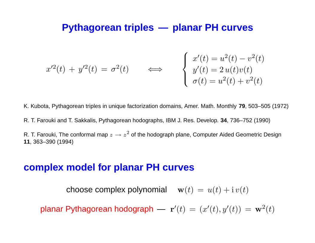
Pythagorean triples — planar PH curves
x′2(t) + y′2(t) = σ2(t) ⇐⇒
x′(t) = u2(t)− v2(t)y′(t) = 2u(t)v(t)σ(t) = u2(t) + v2(t)
K. Kubota, Pythagorean triples in unique factorization domains, Amer. Math. Monthly 79, 503–505 (1972)
R. T. Farouki and T. Sakkalis, Pythagorean hodographs, IBM J. Res. Develop. 34, 736–752 (1990)
R. T. Farouki, The conformal map z → z2 of the hodograph plane, Computer Aided Geometric Design11, 363–390 (1994)
complex model for planar PH curves
choose complex polynomial w(t) = u(t) + i v(t)
planar Pythagorean hodograph — r′(t) = (x′(t), y′(t)) = w2(t)
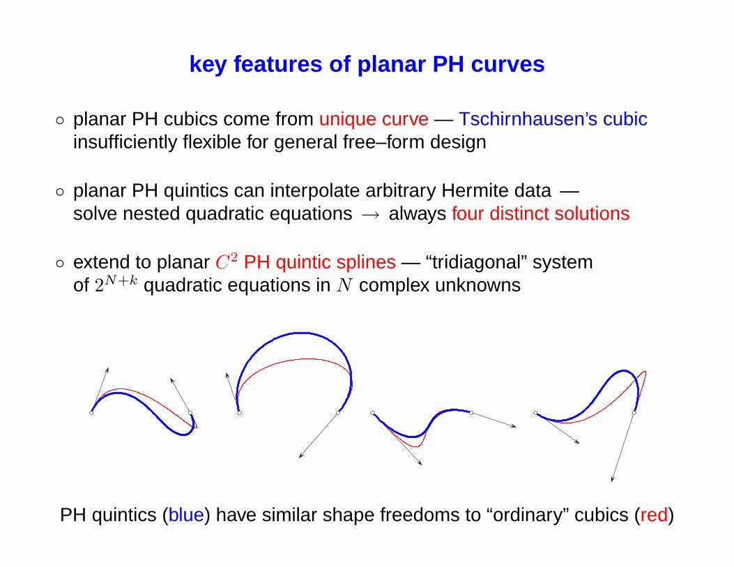
key features of planar PH curves
◦ planar PH cubics come from unique curve — Tschirnhausen’s cubicinsufficiently flexible for general free–form design
◦ planar PH quintics can interpolate arbitrary Hermite data —solve nested quadratic equations → always four distinct solutions
◦ extend to planar C2 PH quintic splines — “tridiagonal” systemof 2N+k quadratic equations in N complex unknowns
PH quintics (blue) have similar shape freedoms to “ordinary” cubics (red)
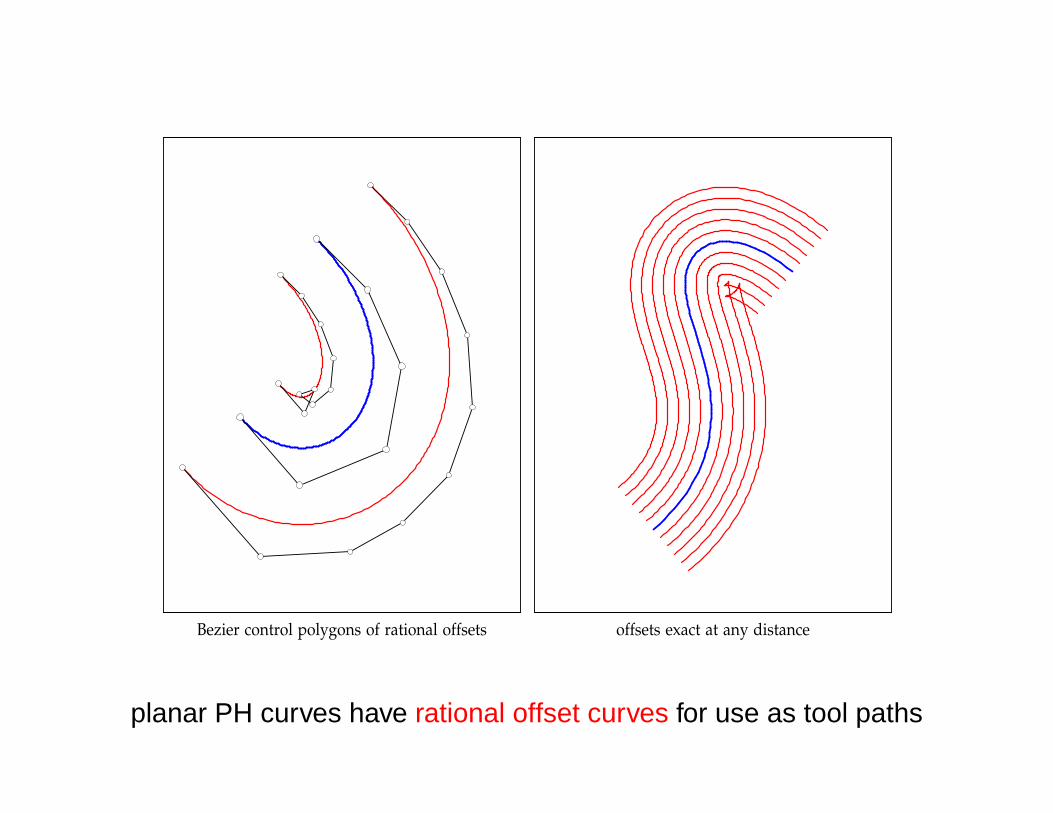
Bezier control polygons of rational offsets offsets exact at any distance
planar PH curves have rational offset curves for use as tool paths
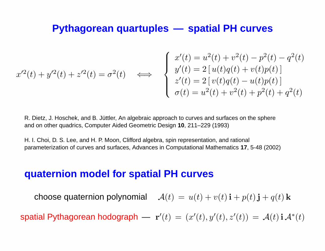
Pythagorean quartuples — spatial PH curves
x′2(t) + y′2(t) + z′2(t) = σ2(t) ⇐⇒
x′(t) = u2(t) + v2(t)− p2(t)− q2(t)y′(t) = 2 [u(t)q(t) + v(t)p(t) ]z′(t) = 2 [ v(t)q(t)− u(t)p(t) ]σ(t) = u2(t) + v2(t) + p2(t) + q2(t)
R. Dietz, J. Hoschek, and B. Juttler, An algebraic approach to curves and surfaces on the sphereand on other quadrics, Computer Aided Geometric Design 10, 211–229 (1993)
H. I. Choi, D. S. Lee, and H. P. Moon, Clifford algebra, spin representation, and rationalparameterization of curves and surfaces, Advances in Computational Mathematics 17, 5-48 (2002)
quaternion model for spatial PH curves
choose quaternion polynomial A(t) = u(t) + v(t) i + p(t) j + q(t)k
spatial Pythagorean hodograph — r′(t) = (x′(t), y′(t), z′(t)) = A(t) iA∗(t)
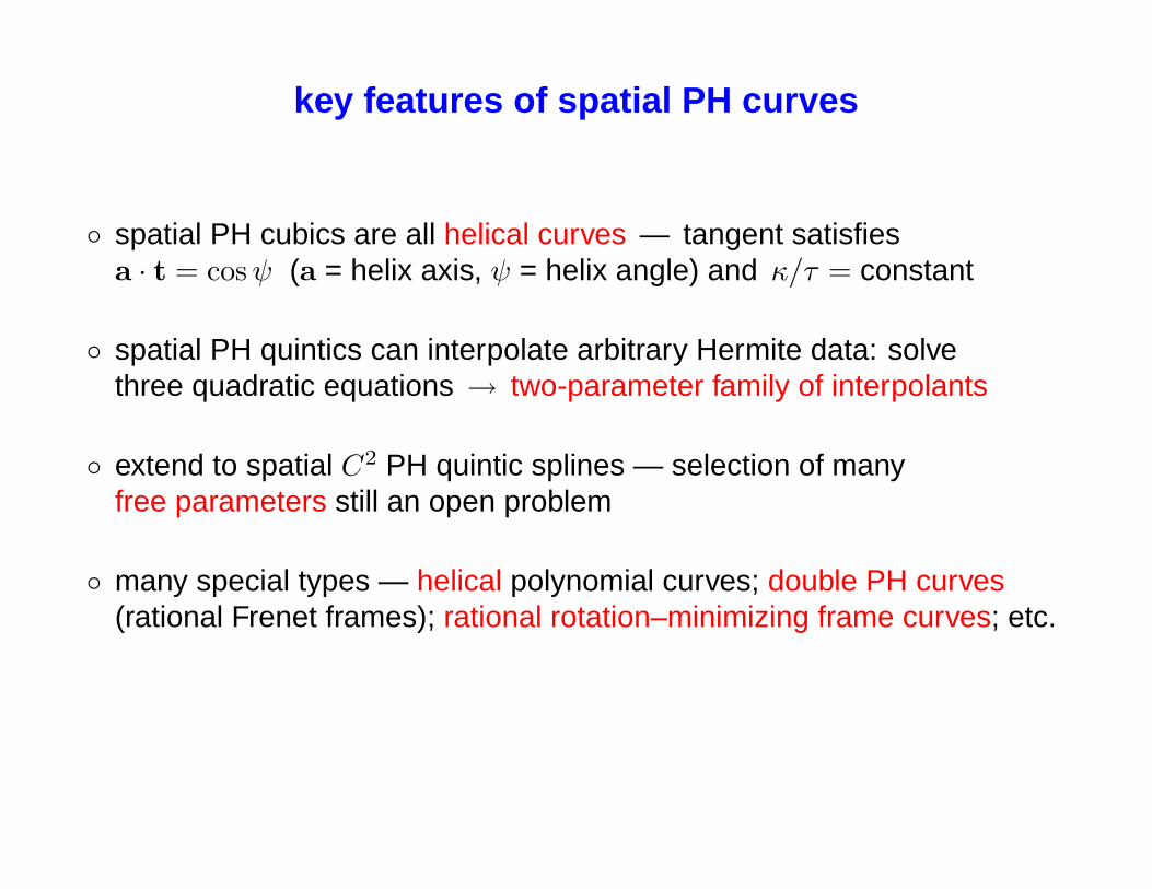
key features of spatial PH curves
◦ spatial PH cubics are all helical curves — tangent satisfiesa · t = cosψ (a = helix axis, ψ = helix angle) and κ/τ = constant
◦ spatial PH quintics can interpolate arbitrary Hermite data: solvethree quadratic equations → two-parameter family of interpolants
◦ extend to spatial C2 PH quintic splines — selection of manyfree parameters still an open problem
◦ many special types — helical polynomial curves; double PH curves(rational Frenet frames); rational rotation–minimizing frame curves; etc.
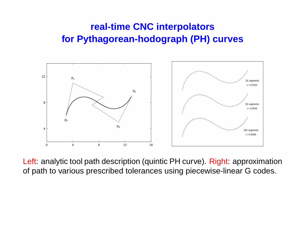
real-time CNC interpolatorsfor Pythagorean-hodograph (PH) curves
0 4 8 12 16
4
8
12
p0
p1
p4
p5
25 segments
ε = 0.0105
50 segments
ε = 0.0025
100 segments
ε = 0.0006
Left: analytic tool path description (quintic PH curve). Right: approximationof path to various prescribed tolerances using piecewise-linear G codes.
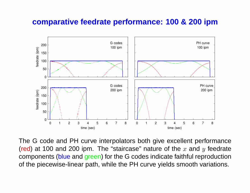
comparative feedrate performance: 100 & 200 ipm
0 1 2 3 4 5 6 7 80
50
100
150
200
time (sec)
feed
rate
(ip
m)
G codes200 ipm
0
50
100
150
200
feed
rate
(ip
m)
G codes100 ipm
0 1 2 3 4 5 6 7 8time (sec)
PH curve200 ipm
PH curve100 ipm
The G code and PH curve interpolators both give excellent performance(red) at 100 and 200 ipm. The “staircase” nature of the x and y feedratecomponents (blue and green) for the G codes indicate faithful reproductionof the piecewise-linear path, while the PH curve yields smooth variations.
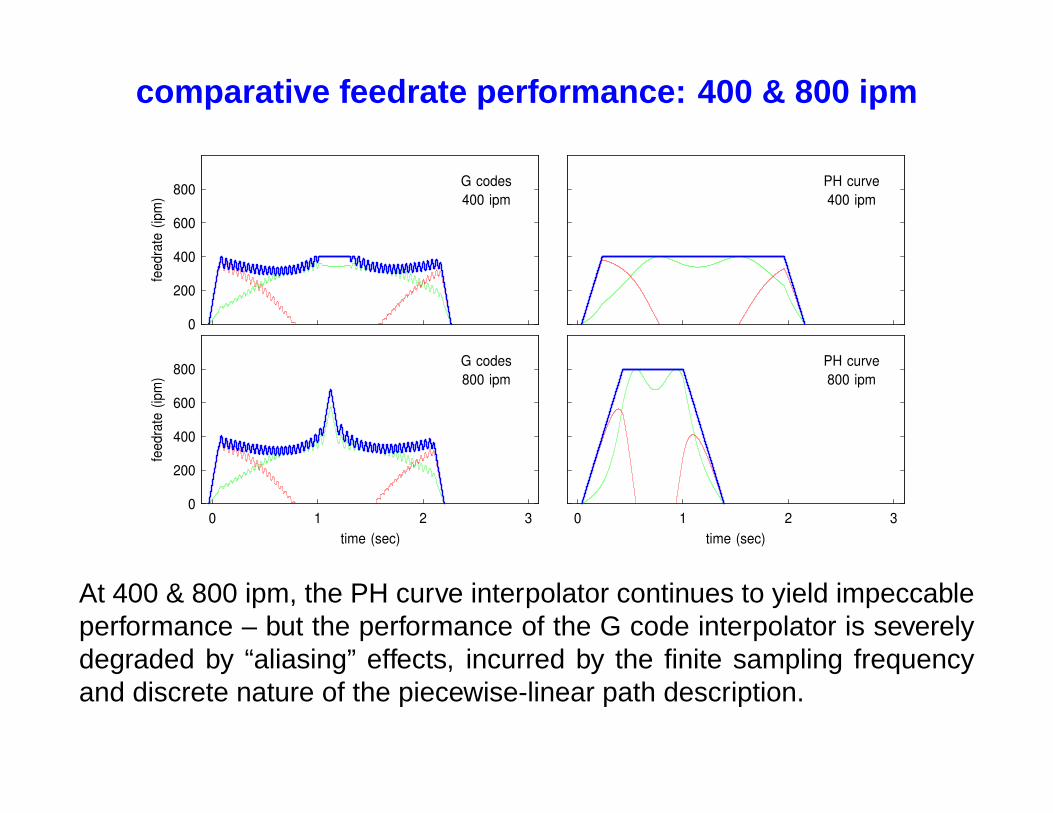
comparative feedrate performance: 400 & 800 ipm
0 1 2 30
200
400
600
800
time (sec)
feed
rate
(ip
m)
G codes800 ipm
0
200
400
600
800
feed
rate
(ip
m)
G codes400 ipm
0 1 2 3time (sec)
PH curve800 ipm
PH curve400 ipm
At 400 & 800 ipm, the PH curve interpolator continues to yield impeccableperformance – but the performance of the G code interpolator is severelydegraded by “aliasing” effects, incurred by the finite sampling frequencyand discrete nature of the piecewise-linear path description.
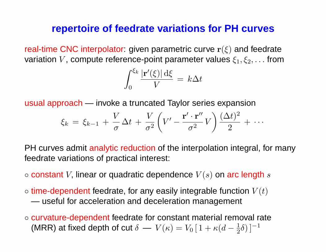
repertoire of feedrate variations for PH curves
real-time CNC interpolator: given parametric curve r(ξ) and feedratevariation V , compute reference-point parameter values ξ1, ξ2, . . . from∫ ξk
0
|r′(ξ)|dξV
= k∆t
usual approach — invoke a truncated Taylor series expansion
ξk = ξk−1 +V
σ∆t +
V
σ2
(V ′ − r′ · r′′
σ2V
)(∆t)2
2+ · · ·
PH curves admit analytic reduction of the interpolation integral, for manyfeedrate variations of practical interest:
◦ constant V, linear or quadratic dependence V (s) on arc length s
◦ time-dependent feedrate, for any easily integrable function V (t)— useful for acceleration and deceleration management
◦ curvature-dependent feedrate for constant material removal rate(MRR) at fixed depth of cut δ — V (κ) = V0 [ 1 + κ(d− 1
2δ) ]−1
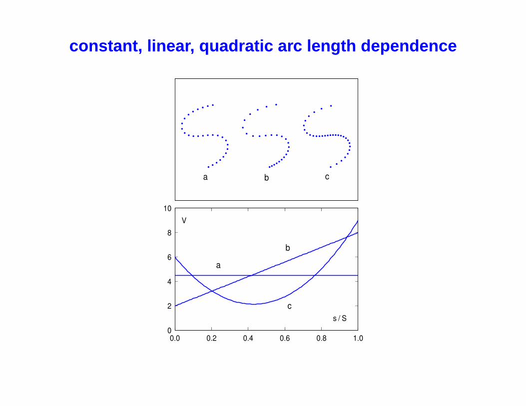
constant, linear, quadratic arc length dependence
0.0 0.2 0.4 0.6 0.8 1.00
2
4
6
8
10
s / S
V
a b c
a
b
c
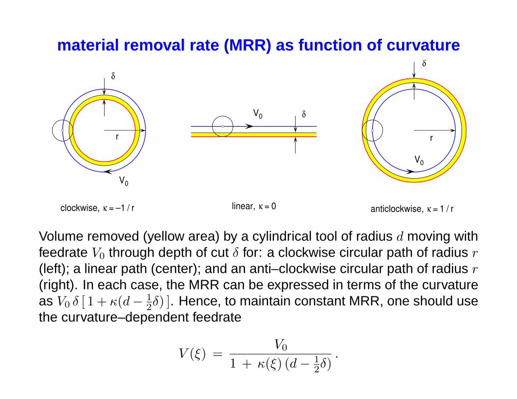
material removal rate (MRR) as function of curvature
r r
δδ
δ
linear, κ = 0 anticlockwise, κ = 1 / rclockwise, κ = –1 / r
V0
V0
V0
Volume removed (yellow area) by a cylindrical tool of radius d moving withfeedrate V0 through depth of cut δ for: a clockwise circular path of radius r(left); a linear path (center); and an anti–clockwise circular path of radius r(right). In each case, the MRR can be expressed in terms of the curvatureas V0 δ [ 1 + κ(d− 1
2δ) ]. Hence, to maintain constant MRR, one should usethe curvature–dependent feedrate
V (ξ) =V0
1 + κ(ξ) (d− 12δ)
.
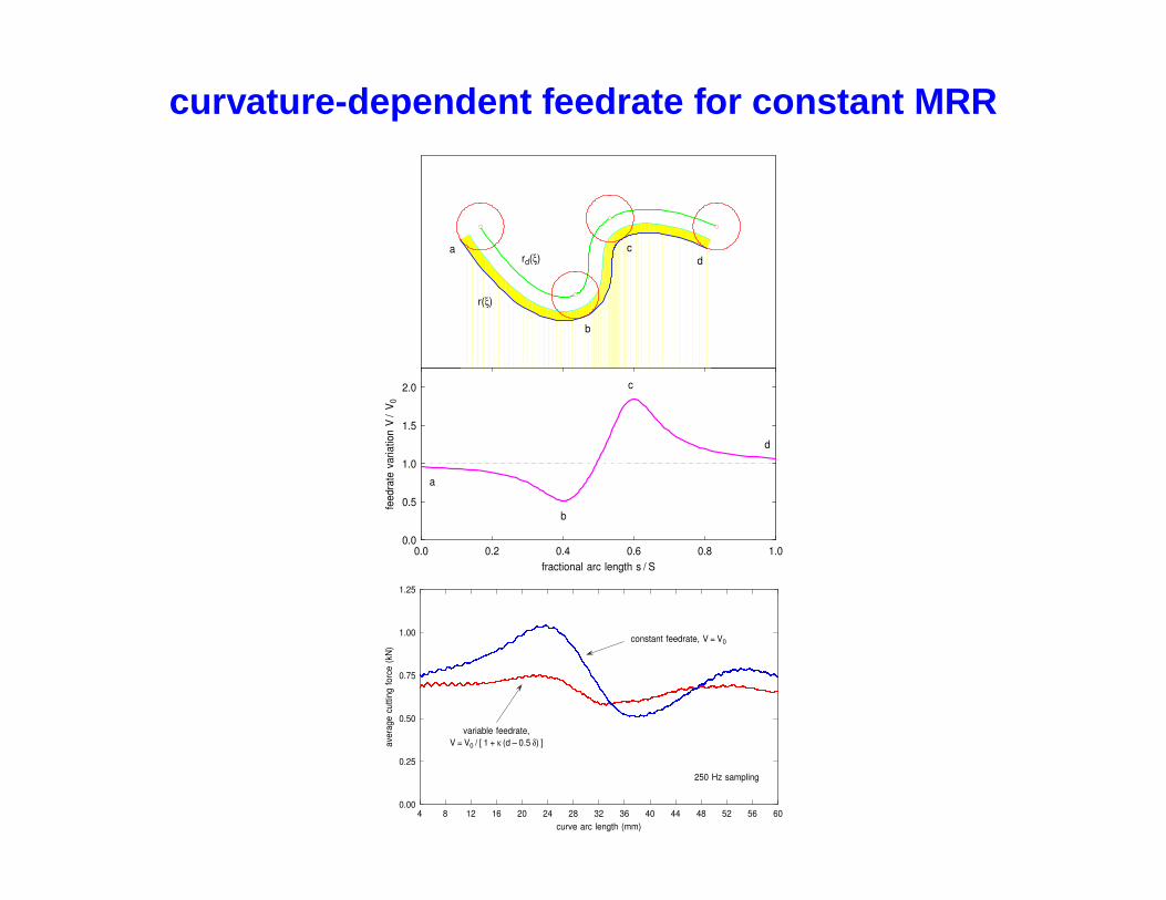
curvature-dependent feedrate for constant MRR
0.0 0.2 0.4 0.6 0.8 1.00.0
0.5
1.0
1.5
2.0
fractional arc length s / S
feed
rate
var
iatio
n V
/V 0
r(ξ)
rd(ξ)a
b
cd
a
b
c
d
4 8 12 16 20 24 28 32 36 40 44 48 52 56 600.00
0.25
0.50
0.75
1.00
1.25
curve arc length (mm)
aver
age
cutti
ng fo
rce
(kN
)
250 Hz sampling
constant feedrate, V = V0
variable feedrate,V = V0 / [ 1 + κ (d – 0.5 δ) ]
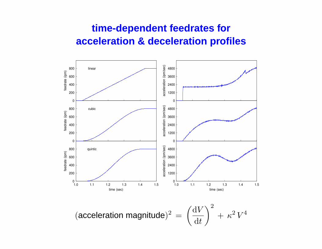
time-dependent feedrates foracceleration & deceleration profiles
quintic
1.0 1.1 1.2 1.3 1.4 1.50
200
400
600
800
time (sec)
feed
rate
(ip
m)
cubic
0
200
400
600
800
feed
rate
(ip
m)
linear
0
200
400
600
800fe
edra
te (ip
m)
1.0 1.1 1.2 1.3 1.4 1.50
1200
2400
3600
4800
time (sec)
acce
lera
tion
(ipm
/sec
)
0
1200
2400
3600
4800
acce
lera
tion
(ipm
/sec
)
0
1200
2400
3600
4800
acce
lera
tion
(ipm
/sec
)
(acceleration magnitude)2 =(
dVdt
)2
+ κ2 V 4
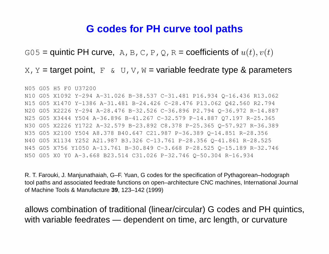
G codes for PH curve tool paths
G05 = quintic PH curve, A,B,C,P,Q,R = coefficients of u(t), v(t)
X,Y = target point, F & U,V,W = variable feedrate type & parameters
N05 G05 H5 F0 U37200N10 G05 X1092 Y-294 A-31.026 B-38.537 C-31.481 P16.934 Q-16.436 R13.062N15 G05 X1470 Y-1386 A-31.481 B-24.426 C-28.476 P13.062 Q42.560 R2.794N20 G05 X2226 Y-294 A-28.476 B-32.526 C-36.896 P2.794 Q-36.972 R-14.887N25 G05 X3444 Y504 A-36.896 B-41.267 C-32.579 P-14.887 Q7.197 R-25.365N30 G05 X2226 Y1722 A-32.579 B-23.892 C8.378 P-25.365 Q-57.927 R-36.389N35 G05 X2100 Y504 A8.378 B40.647 C21.987 P-36.389 Q-14.851 R-28.356N40 G05 X1134 Y252 A21.987 B3.326 C-13.761 P-28.356 Q-41.861 R-28.525N45 G05 X756 Y1050 A-13.761 B-30.849 C-3.668 P-28.525 Q-15.189 R-32.746N50 G05 X0 Y0 A-3.668 B23.514 C31.026 P-32.746 Q-50.304 R-16.934
R. T. Farouki, J. Manjunathaiah, G–F. Yuan, G codes for the specification of Pythagorean–hodographtool paths and associated feedrate functions on open–architecture CNC machines, International Journalof Machine Tools & Manufacture 39, 123–142 (1999)
allows combination of traditional (linear/circular) G codes and PH quintics,with variable feedrates — dependent on time, arc length, or curvature
inverse dynamics problem for path error minimization
inertia (resistance to motion) and damping (frictional energy dissipation)of CNC machine axes prevent exact execution of commanded motion
develop dynamic model of machine/controller system, expressed in termsof linear ordinary differential equations
transform independent variable from the time t to the curve parameter ξ :constant coefficients → polynomial coefficients
revert differential equations: swap input & output dependent variables
solve reverted differential equations for modified input path that, subjectto machine dynamics, exactly yields desired output path
for brevity, consider only x–axis motion (same principles for y, z axes)
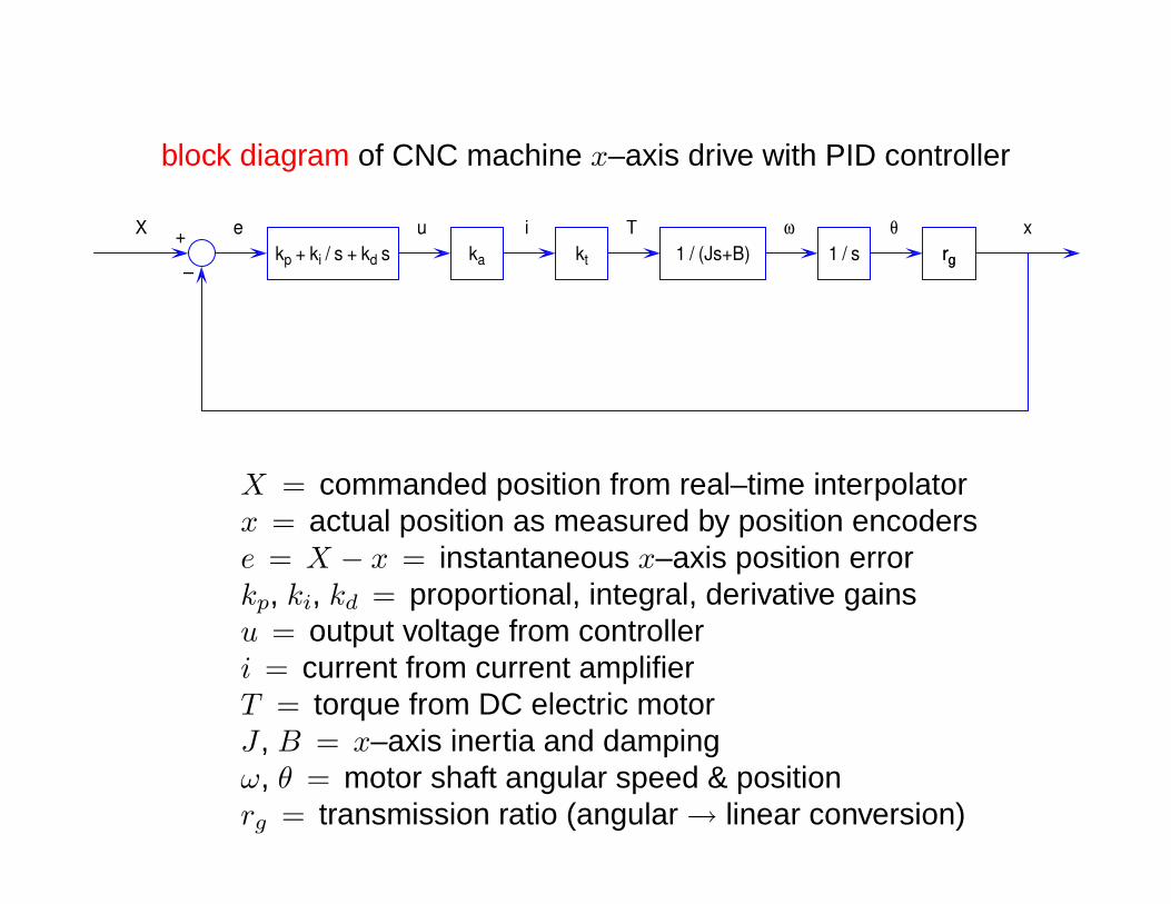
block diagram of CNC machine x–axis drive with PID controller
ka kt
i1 / (Js+B)
T1 / s
ωrg
θ xX ergkp + ki / s + kd s
u+ –
X = commanded position from real–time interpolatorx = actual position as measured by position encoderse = X − x = instantaneous x–axis position errorkp, ki, kd = proportional, integral, derivative gainsu = output voltage from controlleri = current from current amplifierT = torque from DC electric motorJ , B = x–axis inertia and dampingω, θ = motor shaft angular speed & positionrg = transmission ratio (angular → linear conversion)
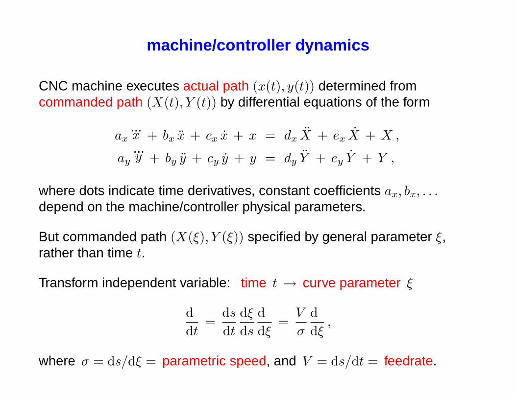
machine/controller dynamics
CNC machine executes actual path (x(t), y(t)) determined fromcommanded path (X(t), Y (t)) by differential equations of the form
ax...x + bx x + cx x + x = dx X + ex X + X ,
ay...y + by y + cy y + y = dy Y + ey Y + Y ,
where dots indicate time derivatives, constant coefficients ax, bx, . . .depend on the machine/controller physical parameters.
But commanded path (X(ξ), Y (ξ)) specified by general parameter ξ,rather than time t.
Transform independent variable: time t → curve parameter ξ
ddt
=dsdt
dξds
ddξ
=V
σ
ddξ,
where σ = ds/dξ = parametric speed, and V = ds/dt = feedrate.
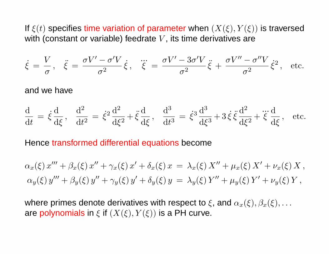
If ξ(t) specifies time variation of parameter when (X(ξ), Y (ξ)) is traversedwith (constant or variable) feedrate V , its time derivatives are
ξ =V
σ, ξ =
σV ′ − σ′V
σ2ξ ,
...ξ =
σV ′ − 3σ′Vσ2
ξ +σV ′′ − σ′′V
σ2ξ2 , etc.
and we have
ddt
= ξddξ,
d2
dt2= ξ2
d2
dξ2+ ξ
ddξ,
d3
dt3= ξ3
d3
dξ3+3 ξ ξ
d2
dξ2+
...ξ
ddξ, etc.
Hence transformed differential equations become
αx(ξ)x′′′ + βx(ξ)x′′ + γx(ξ)x′ + δx(ξ)x = λx(ξ)X ′′ + µx(ξ)X ′ + νx(ξ)X ,
αy(ξ) y′′′ + βy(ξ) y′′ + γy(ξ) y′ + δy(ξ) y = λy(ξ)Y ′′ + µy(ξ)Y ′ + νy(ξ)Y ,
where primes denote derivatives with respect to ξ, and αx(ξ), βx(ξ), . . .are polynomials in ξ if (X(ξ), Y (ξ)) is a PH curve.
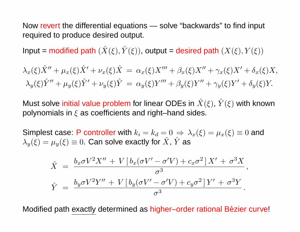
Now revert the differential equations — solve “backwards” to find inputrequired to produce desired output.
Input = modified path (X(ξ), Y (ξ)), output = desired path (X(ξ), Y (ξ))
λx(ξ)X ′′ + µx(ξ)X ′ + νx(ξ)X = αx(ξ)X ′′′ + βx(ξ)X ′′ + γx(ξ)X ′ + δx(ξ)X,
λy(ξ)Y ′′ + µy(ξ)Y ′ + νy(ξ)Y = αy(ξ)Y ′′′ + βy(ξ)Y ′′ + γy(ξ)Y ′ + δy(ξ)Y.
Must solve initial value problem for linear ODEs in X(ξ), Y (ξ) with knownpolynomials in ξ as coefficients and right–hand sides.
Simplest case: P controller with ki = kd = 0 ⇒ λx(ξ) = µx(ξ) ≡ 0 andλy(ξ) = µy(ξ) ≡ 0. Can solve exactly for X, Y as
X =bxσV
2X ′′ + V [ bx(σV ′ − σ′V ) + cxσ2 ]X ′ + σ3X
σ3,
Y =byσV
2Y ′′ + V [ by(σV ′ − σ′V ) + cyσ2 ]Y ′ + σ3Y
σ3.
Modified path exactly determined as higher–order rational Bezier curve!
For more sophisticated PI and PID controllers, obtain first and secondorder differential equations for X, Y .
NOTE: ki 6= 0 ⇒ zero steady–state error and kd 6= 0 ⇒ fast response.
ODEs with polynomial coefficients & right–hand sides do not, in general,admit polynomial solutions.
Need good numerical method to approximate solutions on ξ ∈ [ 0, 1 ] bypolynomial or piecewise–polynomial functions:
• Chebyshev economization methods
• linear least–squares approximation
• interpolation at Chebyshev nodes
• . . . etc.
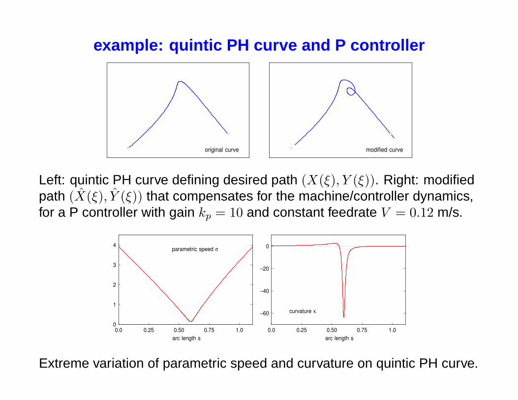
example: quintic PH curve and P controller
original curve modified curve
Left: quintic PH curve defining desired path (X(ξ), Y (ξ)). Right: modifiedpath (X(ξ), Y (ξ)) that compensates for the machine/controller dynamics,for a P controller with gain kp = 10 and constant feedrate V = 0.12 m/s.
0.0 0.25 0.50 0.75 1.0
–60
–40
–20
0
arc length s
curvature κ
0.0 0.25 0.50 0.75 1.00
1
2
3
4
arc length s
parametric speed σ
Extreme variation of parametric speed and curvature on quintic PH curve.
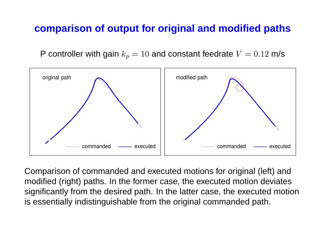
comparison of output for original and modified paths
P controller with gain kp = 10 and constant feedrate V = 0.12 m/s
executedcommanded
original path
executedcommanded
modified path
Comparison of commanded and executed motions for original (left) andmodified (right) paths. In the former case, the executed motion deviatessignificantly from the desired path. In the latter case, the executed motionis essentially indistinguishable from the original commanded path.
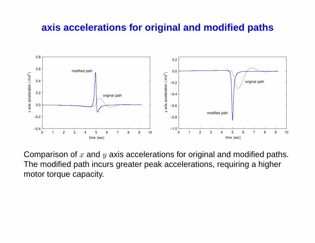
axis accelerations for original and modified paths
0 1 2 3 4 5 6 7 8 9 10–0.4
–0.2
0.0
0.2
0.4
0.6
0.8
time (sec)
x a
xis
acce
lera
tion
(m/s
2)
original path
modified path
0 1 2 3 4 5 6 7 8 9 10–1.0
–0.8
–0.6
–0.4
–0.2
0.0
0.2
time (sec)
y a
xis
acce
lera
tion
(m/s
2)
original path
modified path
Comparison of x and y axis accelerations for original and modified paths.The modified path incurs greater peak accelerations, requiring a highermotor torque capacity.
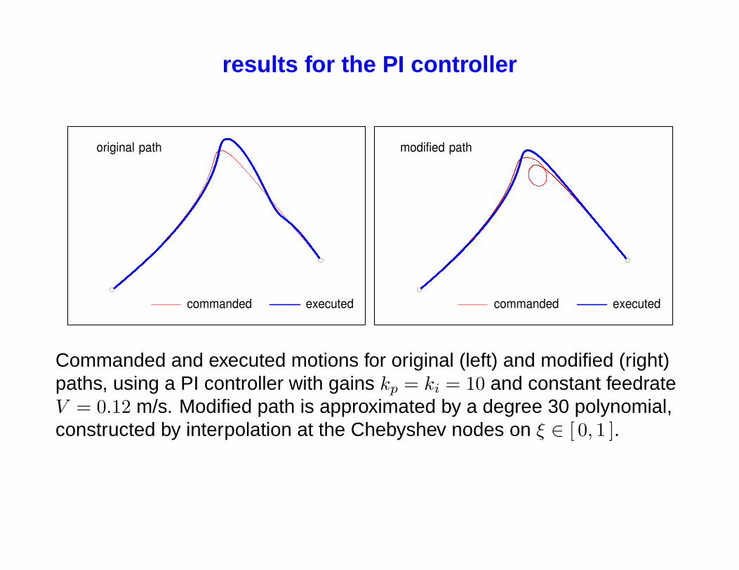
results for the PI controller
executedcommanded
original path
executedcommanded
modified path
Commanded and executed motions for original (left) and modified (right)paths, using a PI controller with gains kp = ki = 10 and constant feedrateV = 0.12 m/s. Modified path is approximated by a degree 30 polynomial,constructed by interpolation at the Chebyshev nodes on ξ ∈ [ 0, 1 ].
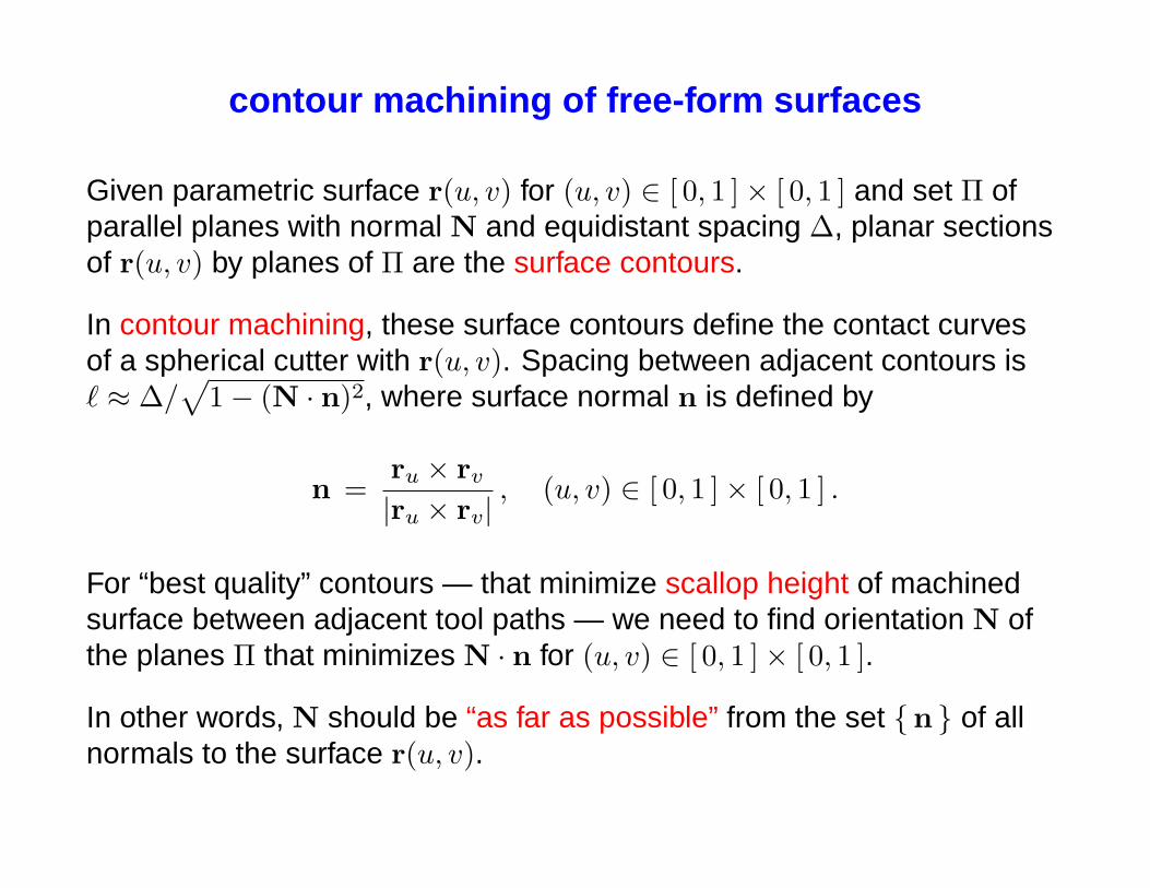
contour machining of free-form surfaces
Given parametric surface r(u, v) for (u, v) ∈ [ 0, 1 ]× [ 0, 1 ] and set Π ofparallel planes with normal N and equidistant spacing ∆, planar sectionsof r(u, v) by planes of Π are the surface contours.
In contour machining, these surface contours define the contact curvesof a spherical cutter with r(u, v). Spacing between adjacent contours is` ≈ ∆/
√1− (N · n)2, where surface normal n is defined by
n =ru × rv
|ru × rv|, (u, v) ∈ [ 0, 1 ]× [ 0, 1 ] .
For “best quality” contours — that minimize scallop height of machinedsurface between adjacent tool paths — we need to find orientation N ofthe planes Π that minimizes N · n for (u, v) ∈ [ 0, 1 ]× [ 0, 1 ].
In other words, N should be “as far as possible” from the set {n } of allnormals to the surface r(u, v).
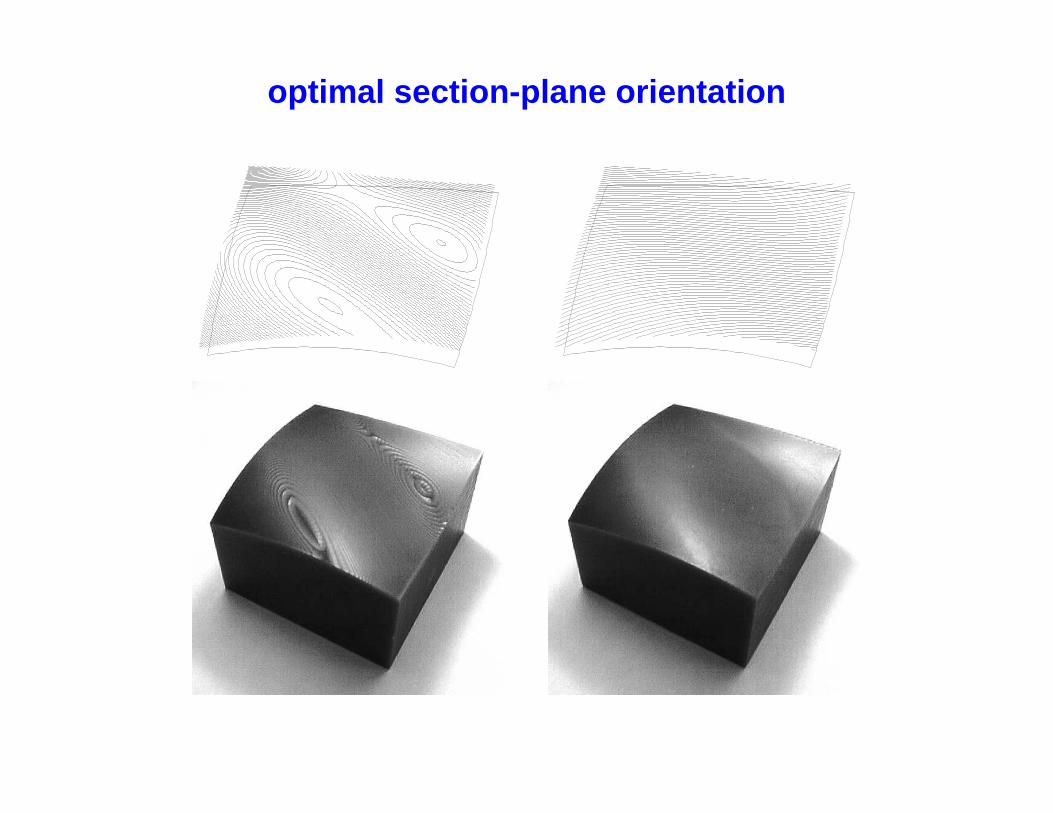
optimal section-plane orientation
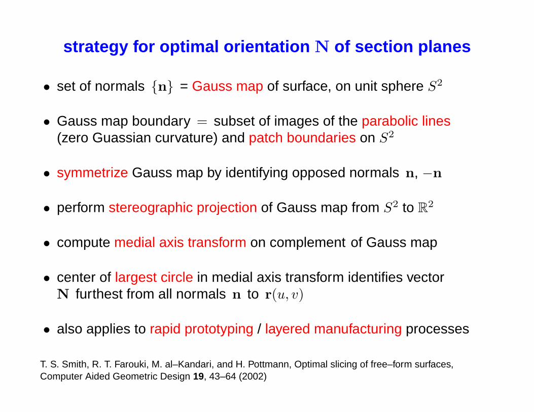
strategy for optimal orientation N of section planes
• set of normals {n} = Gauss map of surface, on unit sphere S2
• Gauss map boundary = subset of images of the parabolic lines(zero Guassian curvature) and patch boundaries on S2
• symmetrize Gauss map by identifying opposed normals n, −n
• perform stereographic projection of Gauss map from S2 to R2
• compute medial axis transform on complement of Gauss map
• center of largest circle in medial axis transform identifies vectorN furthest from all normals n to r(u, v)
• also applies to rapid prototyping / layered manufacturing processes
T. S. Smith, R. T. Farouki, M. al–Kandari, and H. Pottmann, Optimal slicing of free–form surfaces,Computer Aided Geometric Design 19, 43–64 (2002)
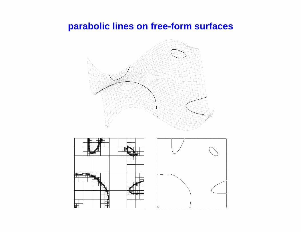
parabolic lines on free-form surfaces
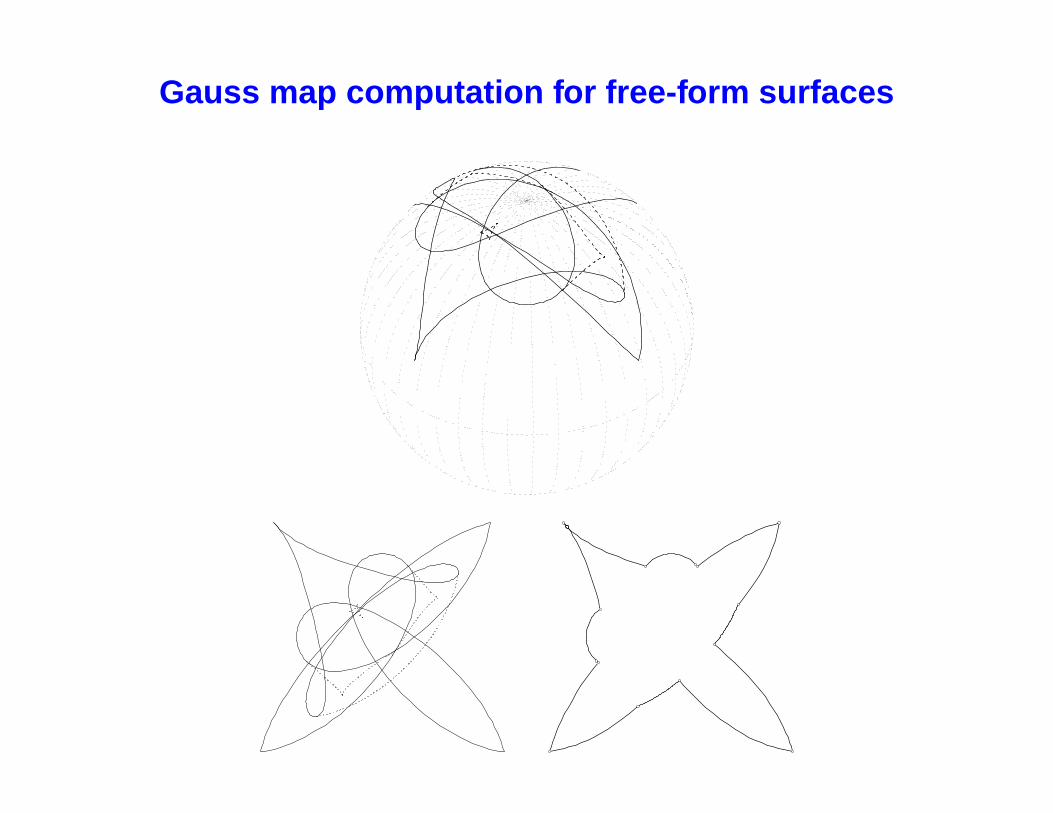
Gauss map computation for free-form surfaces
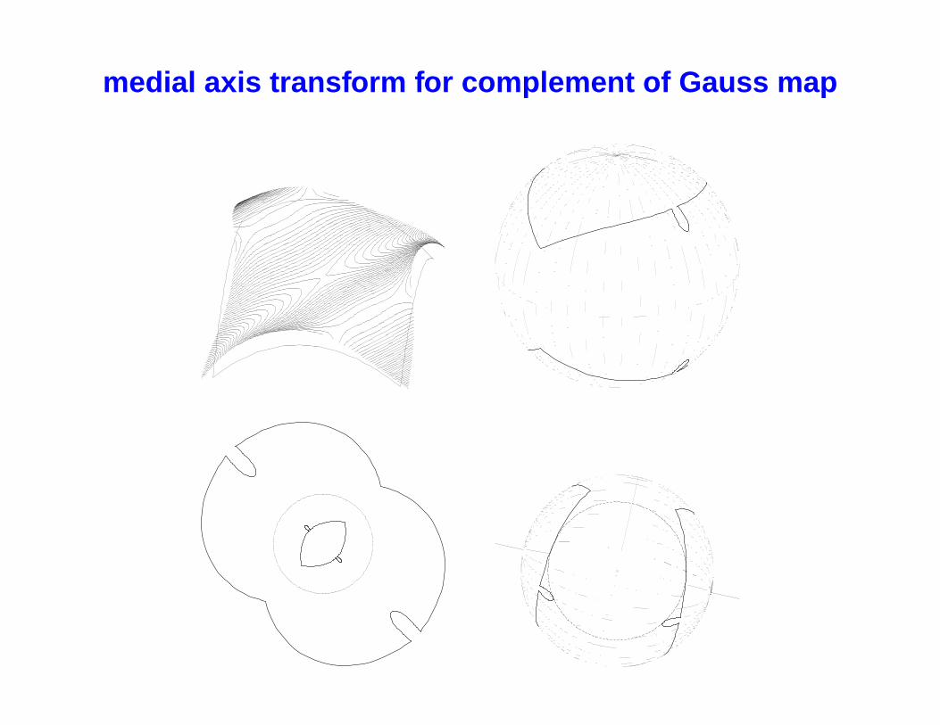
medial axis transform for complement of Gauss map
closure
• Pythagorean-hodograph curves ideally suited to CNC machining
• PH curve real–time interpolator algorithms for feedrates dependenton time, arc length, or curvature
• anayltic curve interpolators give smoother and more accuraterealization of high feedrates and acceleration rates than G codes
• PH curves amenable to solution of inverse dynamics problemsto compensate for inertia & damping of machine axes
• spatial motion planning problems — optimal orientation of sectionplanes for contour machining & use of rotation–minimizing framesin 5–axis machining