Embed Size (px)
Citation preview
REAL-TIME HUMAN HAND POSE ESTIMATION AND TRACKING USING
DEPTH SENSORS
by
Mustafa Furkan Kırac
B.S., Mechanical Engineering, Bogazici University, 2000
M.S., Systems and Control Engineering, Bogazici University, 2002
Submitted to the Institute for Graduate Studies in
Science and Engineering in partial fulfillment of
the requirements for the degree of
Doctor of Philosophy
Graduate Program in Computer Engineering
Bogazici University
2013

ii
REAL-TIME HUMAN HAND POSE ESTIMATION AND TRACKING USING
DEPTH SENSORS
APPROVED BY:
Prof. Lale Akarun . . . . . . . . . . . . . . . . . . .
(Thesis Supervisor)
Assoc. Prof. Taylan Cemgil . . . . . . . . . . . . . . . . . . .
Prof. Tanju Erdem . . . . . . . . . . . . . . . . . . .
Assist. Prof. Albert Ali Salah . . . . . . . . . . . . . . . . . . .
Prof. Bulent Sankur . . . . . . . . . . . . . . . . . . .
DATE OF APPROVAL: 03.09.2013

iii
ACKNOWLEDGEMENTS
I would like to dedicate this thesis to my now passed away grand mother, and
my way-ahead-of-his-time grand father for their invaluable positive effects on me, for
teaching me with unconditional love. I would like to thank my parents for their un-
ending love and support, even sometimes there were kilometers between us. I wish
to thank the following people for having helped me in one way or another during the
course of my thesis. First of all, my supervisor, Prof. Lale Akarun, for having believed
in me for a long time, starting from my master thesis committee. She has envisioned
the direction to be investigated accurately, since 2000. Her constructive criticisms and
encouragements made me feel I have learned a lot during this project. Yunus Emre, for
being a great technical advisor, an awesome friend, and an exceptional coder. Gaye,
for being her, and for her tolerance to Yunus Emre and I, during hard coding hours.
All the members of PILAB, especially Ismail for his wide and spreading creative enthu-
siasm; Alp for extraordinary fast solutions; Barıs Evrim, Barıs Kurt, Nese, Heysem,
and Umut(s) for always studying in the lab, Cem for igniting me. Ozer, for being
an extraordinary friend, for his spreading joy, for our brainstorming sessions, for our
unending ridiculous jokes, and long walks. Prof. Oguz Sunay, Prof. Tanju Erdem, and
Prof. Reha Civanlar; for believing in me, and together with Ozer providing me the be-
ginning of a life-long journey as a member of Computer Science Department of Ozyegin
University. Alihan, Bilgin and Ersin, for their precious talks, long walks, and for being
there. Finally, I would like to thank my thesis committee; Prof. Bulent Sankur for his
very detailed guidance, Prof. Taylan Cemgil for his tolerance to my heuristics, Prof.
Albert Ali Salah for his game changer insights, and Prof. Tanju Erdem for supporting
me during my difficult times.
iv
ABSTRACT
REAL-TIME HUMAN HAND POSE ESTIMATION AND
TRACKING USING DEPTH SENSORS
The human hand has become an important interaction tool in computer systems.
Using the articulated hand skeleton for interaction was a challenge until the develop-
ment of input devices and fast computers. In this thesis, we develop model-based
super real-time methods for articulated human hand pose estimation using depth sen-
sors. We use Randomized Decision Forest (RDF) based methods for feature extraction
and inference from single depth image. We start by implementing shape recognition
using RDFs. We extend the shape recognition by considering a multitude of shapes
in a single image representing different hand regions centered around different joints
of the hand. The regions are utilized for joint position estimation by running mean
shift mode finding algorithm (RDF-C). We combine shape recognition and joint esti-
mation methods in a hybrid structure for boosting the quality. RDFs, when used for
pixel classification are not resistant to self-occlusion. We overcome this by skipping the
classification, and directly inferring the joint positions using regression forests. These
methods assume joints are independent, which is not realistic. Therefore, we conclude
our single image based framework by considering the geometry constraints of the model
(RDF-R+). The accuracies at 10 mm acceptance threshold are acquired for synthetic
and real datasets. Comparing RDF-C and RDF-R+ methods respectively, we report
significant accuracy increase. We finally extend single image methods to tracking dy-
namic gestures. We learn the grasping motion from synthetic data by extracting a
manifold, and fix RDF estimations by projecting them onto the manifold. We then
track the projections by using a Kalman Filter.
v
OZET
DERINLIK ALGILAYICILARI ILE GERCEK ZAMANLI
INSAN EL POZU KESTIRIMI VE IZLEMESI
Insan eli bilgisayar sistemlerinde onemli bir iletisim aracı olmustur. Eklemli
iskelet modelleri ile giris aygıtlarının ve hızlı bilgisayarların gelisimine kadar calısma
yapılamamıstır. Bu tezde derinlik algılayıcıları ile insan el pozu kestirimi icin gercek
zaman otesinde calısan model tabanlı eklem metodları gelistirdik. Derinlik imgesinden
oznitelik ozutleme ve cıkarımı icin Rasgele Karar Agacları (RDF) kullandık. RDF’leri
sekil tanıma icin uygulayarak basladık. Sekil tanımayı aynı derinlik resminde eklemler
etrafında merkezlenmis birden fazla sekli destekler bicimde gelistirdik. Mean shift al-
goritması kullanarak bu bolgelerin merkezlerindeki eklemleri kestirdik (RDF-C). Sekil
tanıma ve eklem kestirimini birlestirip melez agaclarla kaliteyi arttırdık. RDF’ler piksel
tanıma ile kullanıldıgında kapatma durumlarına dayanıklı degiller. Bu problemi tanıma
adımını atlayarak ve eklemleri kestirirken baglanım kullanarak astık. Bu metodlar
gercekci olmayan bicimde eklemleri bagımsız olarak kabul ediyorlar. Bu yuzden tek
resim tabanlı yontemimizi modelin geometrik ozelliklerini kullanarak gelistirdik (RDF-
R+). 10 mm kabul esiginde dogruluk degerlerini sentetik ve gercek veriler uzerinde
hesapladık. RDF-C ve RDF-R+ metodlarını kıyasladıgımızda dogruluk degerlerinin
buyuk artıs gosterdigini gozlemledik. Son olarak, tek resim temelli metodlarımızı di-
namik hareketler izlemek icin gelistirdik. Sentetik veriden kavrama hareketinin mani-
foldunu ogrendik. RDF kestirimlerimizi manifold uzerine izdusumleyerek duzelttik ve
Kalman suzgeci ile izledik.

vi
TABLE OF CONTENTS
ACKNOWLEDGEMENTS . . . . . . . . . . . . . . . . . . . . . . . . . . . . . iii
ABSTRACT . . . . . . . . . . . . . . . . . . . . . . . . . . . . . . . . . . . . . iv
OZET . . . . . . . . . . . . . . . . . . . . . . . . . . . . . . . . . . . . . . . . . v
LIST OF FIGURES . . . . . . . . . . . . . . . . . . . . . . . . . . . . . . . . . ix
LIST OF TABLES . . . . . . . . . . . . . . . . . . . . . . . . . . . . . . . . . . xii
1. INTRODUCTION . . . . . . . . . . . . . . . . . . . . . . . . . . . . . . . . 1
1.1. Motivation . . . . . . . . . . . . . . . . . . . . . . . . . . . . . . . . . . 1
1.2. Definition of the Problem . . . . . . . . . . . . . . . . . . . . . . . . . 2
1.3. Real-time Hand Pose Estimation with Advances in Sensors . . . . . . . 3
1.4. Summary of Contributions . . . . . . . . . . . . . . . . . . . . . . . . . 5
1.5. Organization of the Thesis . . . . . . . . . . . . . . . . . . . . . . . . . 6
2. MODELING OF THE HUMAN HAND . . . . . . . . . . . . . . . . . . . . 7
2.1. Introduction . . . . . . . . . . . . . . . . . . . . . . . . . . . . . . . . . 7
2.1.1. Hand Modeling in Computer Graphics . . . . . . . . . . . . . . 9
2.1.2. Hand Modeling in Medical Research . . . . . . . . . . . . . . . 10
2.1.3. Hand Modeling in Computer Vision . . . . . . . . . . . . . . . . 10
2.2. A Skeleton Model for the Human Hand . . . . . . . . . . . . . . . . . . 11
2.3. Customization for Different Hands . . . . . . . . . . . . . . . . . . . . 13
3. BACKGROUND . . . . . . . . . . . . . . . . . . . . . . . . . . . . . . . . . 14
3.1. Summary . . . . . . . . . . . . . . . . . . . . . . . . . . . . . . . . . . 21
4. SHAPE CLASSIFICATION FROM SINGLE DEPTH IMAGE . . . . . . . . 22
4.1. Randomized Decision Forest (RDF) . . . . . . . . . . . . . . . . . . . . 22
4.2. Pixel Training and Classification using RDF (RDF-C) . . . . . . . . . . 23
4.3. Shape Recognition using Randomized Decision Forest for Pixel Classifi-
cation (RDF-C) . . . . . . . . . . . . . . . . . . . . . . . . . . . . . . . 25
4.4. Randomized Decision Forest for Shape Classification (RDF-S) . . . . . 26
4.4.1. Shape Classification Performance . . . . . . . . . . . . . . . . . 26
4.4.2. Shape Classification Results . . . . . . . . . . . . . . . . . . . . 27
5. HAND POSE ESTIMATION FROM SINGLE DEPTH IMAGE USING PIXEL

vii
CLASSIFICATION . . . . . . . . . . . . . . . . . . . . . . . . . . . . . . . . 29
5.1. Hand Pose Estimation using Randomized Decision Forest for Classifica-
tion (RDF-C) . . . . . . . . . . . . . . . . . . . . . . . . . . . . . . . . 29
5.2. Hand Pose Estimation from Single Depth Image using Hybrid Classifi-
cation Forests (RDF-H) . . . . . . . . . . . . . . . . . . . . . . . . . . . 31
5.2.1. Pose Clustering and Shape Classification Forest (SCF) . . . . . 33
5.2.2. Pose Estimation with Pose Classification Forests (PCF) . . . . . 36
5.2.3. Pose Estimation Using a Hybrid RDF Network (RDF-H) . . . . 36
5.2.4. Forest Parameter Selection . . . . . . . . . . . . . . . . . . . . . 37
5.2.5. Datasets . . . . . . . . . . . . . . . . . . . . . . . . . . . . . . . 37
5.2.6. Shape Classification Performance . . . . . . . . . . . . . . . . . 39
5.2.7. Hand Pose Estimation . . . . . . . . . . . . . . . . . . . . . . . 39
5.2.8. Results . . . . . . . . . . . . . . . . . . . . . . . . . . . . . . . . 41
6. HAND POSE ESTIMATION WITH REGRESSION BASED METHODS . . 44
6.1. Hand Pose Estimation using Randomized Decision Forest for Regression
(RDF-R) . . . . . . . . . . . . . . . . . . . . . . . . . . . . . . . . . . . 45
6.1.1. Training of the Joint Positions . . . . . . . . . . . . . . . . . . . 45
6.1.2. Direct Joint Position Estimation using RDF-R . . . . . . . . . . 47
6.2. Hierarchical Mode Selection using Geometry Constraints (RDF-R+) . . 48
6.3. Data Generation and the Datasets . . . . . . . . . . . . . . . . . . . . 52
6.4. Parameter Selection . . . . . . . . . . . . . . . . . . . . . . . . . . . . . 55
6.4.1. The Effect of the Forest Size . . . . . . . . . . . . . . . . . . . . 56
6.4.2. The Effect of the Tree Depth . . . . . . . . . . . . . . . . . . . 56
6.4.3. The Effect of the Probe Distance . . . . . . . . . . . . . . . . . 58
6.4.4. The Effect of the Depth Threshold . . . . . . . . . . . . . . . . 58
6.4.5. The Effect of the Mean Shift Bandwidth . . . . . . . . . . . . . 59
6.5. Hand Pose Estimation Test Results . . . . . . . . . . . . . . . . . . . . 59
6.5.1. CROP Dataset . . . . . . . . . . . . . . . . . . . . . . . . . . . 60
6.5.2. Rock-Paper-Scissors-Lizard-Spock (RPSLS) Dataset . . . . . . . 62
6.5.3. ASL Finger Spelling Dataset (SURREY) . . . . . . . . . . . . . 64
6.5.4. Results . . . . . . . . . . . . . . . . . . . . . . . . . . . . . . . . 67
7. TRACKING DYNAMIC HAND GESTURES . . . . . . . . . . . . . . . . . 70

viii
7.1. Gaussian Processes . . . . . . . . . . . . . . . . . . . . . . . . . . . . . 70
7.2. Gaussian Process Latent Variable Models (GPLVM) . . . . . . . . . . . 72
7.3. Pose Representation Favorable for Dimensionality Reduction . . . . . . 74
7.4. Learning the 2D Gesture Manifold using GPLVM . . . . . . . . . . . . 75
7.5. Projecting the Pose Observations onto the Gesture Manifold . . . . . . 76
7.6. Kalman Tracker on the 2D Pose Manifold . . . . . . . . . . . . . . . . 76
7.7. Experiments . . . . . . . . . . . . . . . . . . . . . . . . . . . . . . . . . 77
7.8. Results . . . . . . . . . . . . . . . . . . . . . . . . . . . . . . . . . . . . 78
8. CONCLUSIONS AND FUTURE WORK . . . . . . . . . . . . . . . . . . . . 84
8.1. Summary of the Thesis Contributions . . . . . . . . . . . . . . . . . . . 84
8.2. Conclusions . . . . . . . . . . . . . . . . . . . . . . . . . . . . . . . . . 86
8.3. Directions for Future Works . . . . . . . . . . . . . . . . . . . . . . . . 88
8.3.1. Theoretical Investigation . . . . . . . . . . . . . . . . . . . . . . 88
8.3.2. Evaluation . . . . . . . . . . . . . . . . . . . . . . . . . . . . . . 89
REFERENCES . . . . . . . . . . . . . . . . . . . . . . . . . . . . . . . . . . . . 90
ix
LIST OF FIGURES
Figure 1.1. Problem definition. . . . . . . . . . . . . . . . . . . . . . . . . . . 2
Figure 2.1. Anatomy of the human hand. . . . . . . . . . . . . . . . . . . . . 8
Figure 2.2. The 3D hand skeleton model and its labeled parts. . . . . . . . . . 12
Figure 4.1. Depth responses of features. . . . . . . . . . . . . . . . . . . . . . 24
Figure 4.2. Illustration of an RDF classification of a pixel. . . . . . . . . . . . 25
Figure 4.3. Sample RDF-S training images. . . . . . . . . . . . . . . . . . . . 26
Figure 4.4. Overview of the RDF-S based pixel training and shape classification. 27
Figure 4.5. Confusion matrix for the ASL letter classification task using SCF. 28
Figure 4.6. Main cause for error during hand shape classification. . . . . . . . 28
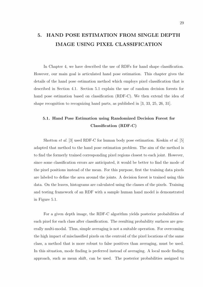
Figure 5.1. Overview of the RDF-C based pixel training and joint estimation. 30
Figure 5.2. Overview of the mean shift convergence during joint estimation. . 32
Figure 5.3. Hand pose estimation process. . . . . . . . . . . . . . . . . . . . . 33
Figure 5.4. Flowchart of randomized hybrid decision forests (RDF-H). . . . . 34
Figure 5.5. Different types of hybrid RDF networks. . . . . . . . . . . . . . . 38
Figure 5.6. Problems of RDFs for pixel classification. . . . . . . . . . . . . . . 43
x
Figure 6.1. Training joint positions. . . . . . . . . . . . . . . . . . . . . . . . . 45
Figure 6.2. Direct estimation of joint positions. . . . . . . . . . . . . . . . . . 46
Figure 6.3. Sample multi-modal vote distributions for three different joints. . . 48
Figure 6.4. Preliminary comparison of classification and regression based meth-
ods. . . . . . . . . . . . . . . . . . . . . . . . . . . . . . . . . . . . 49
Figure 6.5. Improvement of RDF-R+ method over RDF-R shown for tip of the
index finger. . . . . . . . . . . . . . . . . . . . . . . . . . . . . . . 52
Figure 6.6. Sample frames from the TRAIN dataset. . . . . . . . . . . . . . . 54
Figure 6.7. Effect of the forest size. . . . . . . . . . . . . . . . . . . . . . . . . 55
Figure 6.8. Effect of the tree depth. . . . . . . . . . . . . . . . . . . . . . . . . 56
Figure 6.9. Effect of the probe distance. . . . . . . . . . . . . . . . . . . . . . 57
Figure 6.10. Effect of the bandwidths of joints. . . . . . . . . . . . . . . . . . . 58
Figure 6.11. Effect of the tree depth on the recognition time. . . . . . . . . . . 59
Figure 6.12. Effect of the tree depth on the training time. . . . . . . . . . . . . 60
Figure 6.13. CMC curve for the TRAIN dataset. . . . . . . . . . . . . . . . . . 61
Figure 6.14. CMC curve for the CROP dataset. . . . . . . . . . . . . . . . . . . 62
Figure 6.15. CMC curve for the RPSLS dataset. . . . . . . . . . . . . . . . . . 63
xi
Figure 6.16. CMC curve for the SURREY dataset. . . . . . . . . . . . . . . . . 64
Figure 6.17. Sample depth images from SURREY dataset. . . . . . . . . . . . . 65
Figure 6.18. Joint estimation illustrations in the test datasets. . . . . . . . . . 68
Figure 6.19. Joint estimation illustrations in the SURREY dataset. . . . . . . . 69
Figure 7.1. Grasping gesture of a hand demonstrated. . . . . . . . . . . . . . . 80
Figure 7.2. 2D manifold captured from a 50 frame grasping animation. . . . . 81
Figure 7.3. Illustration of projection onto the manifold using local search grid. 81
Figure 7.4. GPLVM convergence. . . . . . . . . . . . . . . . . . . . . . . . . . 82
Figure 7.5. Effects of the Gaussian depth noise. . . . . . . . . . . . . . . . . . 83
Figure 7.6. General direction of the tracked animations over the manifold. . . 83

xii
LIST OF TABLES
Table 3.1. Overview of the relationship between embedding algorithms. . . . 21
Table 5.1. Per pixel classification rates of each hand pose estimation method. 40
Table 5.2. Optimal SCT and PCT heights for different number of clusters. . . 41
Table 6.1. Performances of methods for each sign in SURREY dataset. . . . . 66
Table 6.2. Performances of methods for each subject in SURREY dataset. . . 67
Table 6.3. Acceptance rates for the threshold of 10 mm. . . . . . . . . . . . . 67
Table 7.1. Errors of the different methods in mm. . . . . . . . . . . . . . . . . 78
1
1. INTRODUCTION
1.1. Motivation
An important area of research for the last four decades has been human computer
interaction. Improvement of work efficiency and quality depends on the enhancement
of communication between humans and computers. For that reason, new mice and key-
boards are still being designed. In spite of the new designs, the use of classical input
devices has become a bottleneck when compared to the capabilities of today’s com-
puters. Natural interfaces which make use of speech, touch, and gestures are sought.
Speech recognition has been widely used and has proved its success in recognizing a
multitude of languages. Touch interfaces have become mainstream with the invention
of touch enabled LCD tablets. After the release of multi-touch enabled devices, touch-
ing has become a big part of our lives. Even babies are able to touch and pan these
devices before they are able to talk. However, the real breakthrough will be through
the use of the human hand gestures as an input device.
Gesture based communication is very intuitive for humans. A simple way to
employ gesture recognition is by tracking the position of hands and detecting a gesture.
Detecting and tracking the centers of naked hands are relatively simpler when compared
to detecting the exact configuration of the articulated pose. Unfortunately, most of
the hand gestures require the exact detection of the hand pose and tracking the pose
variations in a robust fashion. Even in the presence of powerful CPUs, articulated
hand pose extraction is a very difficult problem. Moreover, the hand is a small limb
that produces self-occluded poses during gesture performance.
With the introduction of inexpensive depth cameras, the human computer inter-
action field has been revolutionized; and it is now feasible to establish methods em-
ploying computer vision based interaction. Bypassing the illumination based problems
encountered on the images captured by conventional cameras, new depth cameras have
made it possible to establish very fast and less power hungry methods. Unfortunately,
2
inexpensive depth cameras that are widely used still work on low resolution.
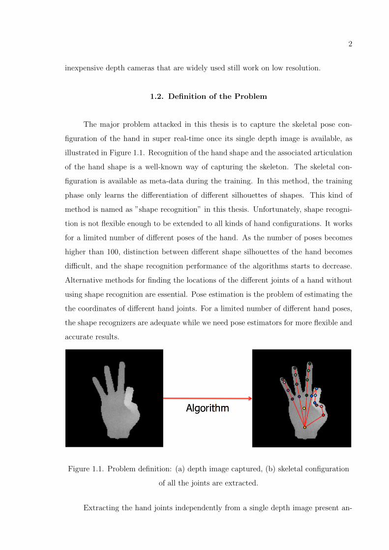
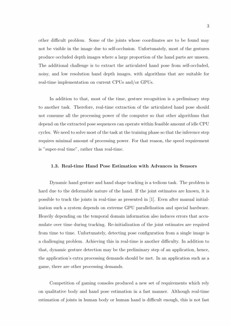
1.2. Definition of the Problem
The major problem attacked in this thesis is to capture the skeletal pose con-
figuration of the hand in super real-time once its single depth image is available, as
illustrated in Figure 1.1. Recognition of the hand shape and the associated articulation
of the hand shape is a well-known way of capturing the skeleton. The skeletal con-
figuration is available as meta-data during the training. In this method, the training
phase only learns the differentiation of different silhouettes of shapes. This kind of
method is named as ”shape recognition” in this thesis. Unfortunately, shape recogni-
tion is not flexible enough to be extended to all kinds of hand configurations. It works
for a limited number of different poses of the hand. As the number of poses becomes
higher than 100, distinction between different shape silhouettes of the hand becomes
difficult, and the shape recognition performance of the algorithms starts to decrease.
Alternative methods for finding the locations of the different joints of a hand without
using shape recognition are essential. Pose estimation is the problem of estimating the
the coordinates of different hand joints. For a limited number of different hand poses,
the shape recognizers are adequate while we need pose estimators for more flexible and
accurate results.
Figure 1.1. Problem definition: (a) depth image captured, (b) skeletal configuration
of all the joints are extracted.
Extracting the hand joints independently from a single depth image present an-
3
other difficult problem. Some of the joints whose coordinates are to be found may
not be visible in the image due to self-occlusion. Unfortunately, most of the gestures
produce occluded depth images where a large proportion of the hand parts are unseen.
The additional challenge is to extract the articulated hand pose from self-occluded,
noisy, and low resolution hand depth images, with algorithms that are suitable for
real-time implementation on current CPUs and/or GPUs.
In addition to that, most of the time, gesture recognition is a preliminary step
to another task. Therefore, real-time extraction of the articulated hand pose should
not consume all the processing power of the computer so that other algorithms that
depend on the extracted pose sequences can operate within feasible amount of idle CPU
cycles. We need to solve most of the task at the training phase so that the inference step
requires minimal amount of processing power. For that reason, the speed requirement
is ”super-real time”, rather than real-time.
1.3. Real-time Hand Pose Estimation with Advances in Sensors
Dynamic hand gesture and hand shape tracking is a tedious task. The problem is
hard due to the deformable nature of the hand. If the joint estimates are known, it is
possible to track the joints in real-time as presented in [1]. Even after manual initial-
ization such a system depends on extreme GPU parallelization and special hardware.
Heavily depending on the temporal domain information also induces errors that accu-
mulate over time during tracking. Re-initialization of the joint estimates are required
from time to time. Unfortunately, detecting pose configuration from a single image is
a challenging problem. Achieving this in real-time is another difficulty. In addition to
that, dynamic gesture detection may be the preliminary step of an application, hence,
the application’s extra processing demands should be met. In an application such as a
game, there are other processing demands.
Competition of gaming consoles produced a new set of requirements which rely
on qualitative body and hand pose estimation in a fast manner. Although real-time
estimation of joints in human body or human hand is difficult enough, this is not fast
4
enough from the perspective of gaming industry. Gaming consoles need great amounts
of power to be allocated normally for running the artificial intelligence logic of the
game and supporting the game scenario by generating realistic computer graphics.
These tasks normally spend most of the processing power already. Hence, in reality
game developers need every bit of CPU/GPU cycle for squeezing all the power from the
console for providing a competitive and profitable game. Human body and hand pose
estimation must be solved not in real-time but in super real-time, freeing most of the
power of the CPU/GPU to the game itself. Unfortunately, preliminary preprocessing
step of foreground and background segmentation is an involved task on its own when
working with color cameras. Background clutter poses a challenging computer vision
problem and cannot be solved in super real-time using today’s computers. Depth
sensors have provided an easy solution to this problem since they are both bypassing
the illumination problem and the background segmentation problem. Unfortunately,
depth sensors were quite expensive, which is not acceptable by game industry, and they
were gathering low resolution imagery. Recently, new cost-efficient depth sensors [2]
have provided a very cost effective solution to this problem. They used structured infra-
red pattern projection to the environment from which they rendered the environment’s
depth map in real time. The sensor is very cheap and is bundled with Microsoft Xbox
Gaming Console starting from 2011.
Recent advances have shown that using random classification forests on depth
images is a suitable choice for hand pose skeleton extraction, since the recognition
phase is very fast and requires minimal time complexity. A method which works
on single depth images for human body pose estimation has been presented by [3]
and revolutionized the game industry with the help of Kinect. Randomized decision
trees are demonstrated for their extreme parallelism, resilience to over-fitting, and
quality estimations as presented in [4]. Since both quality tracking and automatic
initialization of the hand both demand good and fast single frame observations, we
choose an adaptation of the randomized forest methodology to human hand as shown
in [5].
5
1.4. Summary of Contributions
The basic idea explored in this thesis is that the notion of fast joint estimation
of articulated shapes can be, and should be, learned from synthetic examples of an
articulated model. Specifically, we develop new approaches that learn an embedding
of the 3D data where real data performance of the learned model is fast and high. We
start by modeling the human hand in 3D by rigging a skeleton to it. The created hand
synthesizer is capable of representing most configurations that a human hand can be
in. A crucial practical advantage of the synthesizer approach is that any articulated 3D
model which is represented by a 3D mesh model with a skeleton can be animated for
generating big amounts of qualitative synthetic training samples, which in turn can be
used for training an expert suitable for parallel recognition. In some of the applications
reported here, we use our training approach, and achieve state-of-the-art performance
in super real-time.
We then develop and implement a family of algorithms for learning such an
embedding. The algorithms offer a trade-off between simplicity and speed of learning
on the one hand and accuracy and flexibility of the learned concept on the other hand.
We then describe four applications of our learning approach in computer vision: for a
classification task of different shape regions by visual similarity, for a pixel classification
based hand pose estimation, for a regression task of estimating articulated human hand
pose from images, and for a tracking task of specific human hand gesture from videos.
In the context of single frame estimation by regression, the novelty of our approach
is that it relies on learning an embedding that directly reflects model’s constraints in
the target space by using multi-modality of individual estimates of different joints. For
instance, in the case of the human hand, this means that the estimated coordinates of
different joints are always compatible with the bone hierarchy and the length of bones
of the object.
In the context of tracking, we propose a novel embedding which represents both
the prior knowledge of a dynamic gesture and the constraints of the model. Tracking

6
runs on the extracted manifold using a standard Kalman Filter that extremely improves
the joint estimation accuracy if the possible gestures are known beforehand.
1.5. Organization of the Thesis
Chapter 3 provides the background for the thesis research. It describes the prior
work in related areas, with particular emphasis on the two ideas that inspired our
learning approach: randomized forests and manifold extraction for dynamic gestures.
Chapter 2 mentions about the 3D model designed for generating synthetic training
data. Chapter 4 describes the basic randomized decision forest usage for detecting
shapes from depth images. Armed with these algorithms we develop super real-time
approaches for two computer vision domains. In Chapter 5 and Chapter 6 we describe
methods for estimating articulated pose of human hand figure from a single depth
image. In Chapter 7 a method for extracting non-linear manifolds is utilized for track-
ing pre-learned dynamic gestures. We conclude with the discussion of the presented
approaches and the most important directions for future work in Chapter 8.
7
2. MODELING OF THE HUMAN HAND
In this thesis, we study on fitting a hierarchical model to a single depth camera
image of a human hand and track the articulated motion during a specific dynamic
gesture. Human hand is a highly deformable object. Labeling 3D coordinates of hand
joints in depth images is a tedious task. Moreover, inferring the 3D coordinates from
a single depth image is a hard problem even for a human. The amount of data that
is necessary for a qualitative training is vast, hence, manual labeling is infeasible.
Synthetic data generation has already been considered by [6] and found to be effective,
even better than real data at times. Being able to generate synthetic human hand data
requires a detailed study of 3D modeling and animation. Fortunately once a synthesizer
is designed, the difficult problem of collecting training data along with ground truth
labels is achieved. In this chapter, we describe the development of a 3D human hand
rigged with a skeleton that can be animated so that it can represent the poses of a real
human hand.
2.1. Introduction
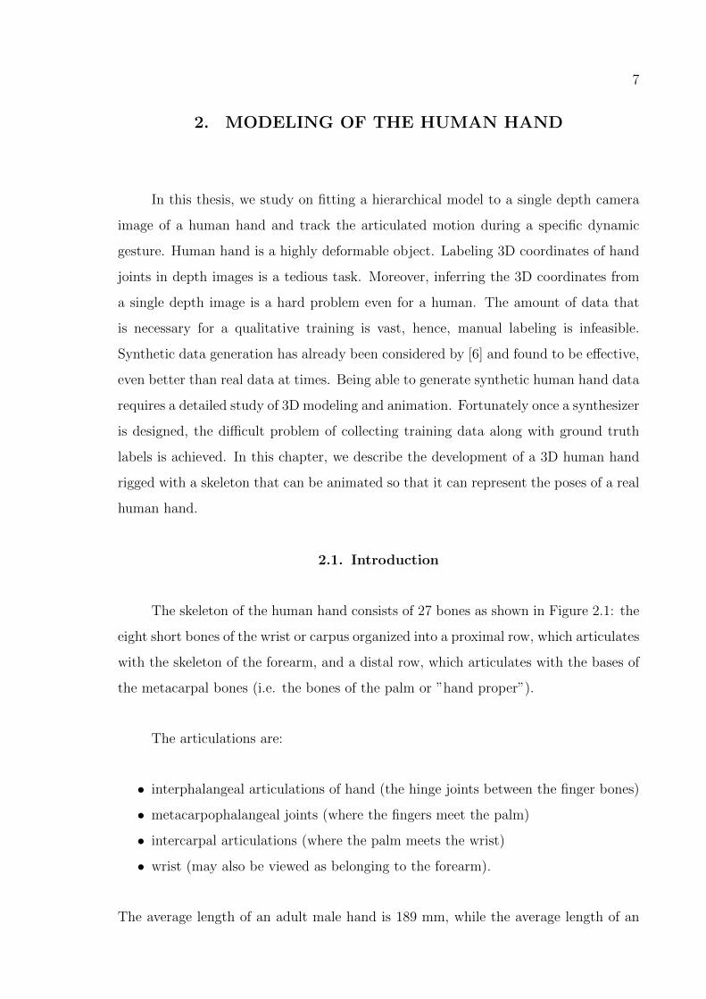
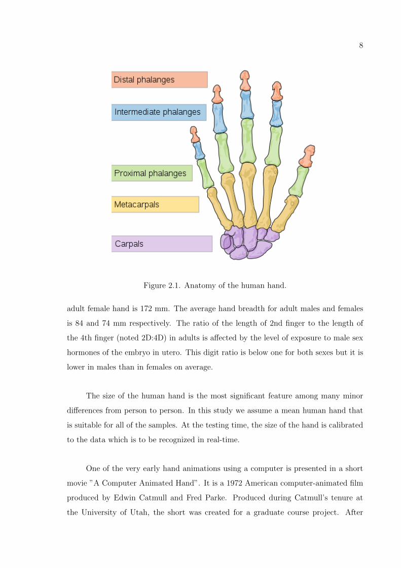
The skeleton of the human hand consists of 27 bones as shown in Figure 2.1: the
eight short bones of the wrist or carpus organized into a proximal row, which articulates
with the skeleton of the forearm, and a distal row, which articulates with the bases of
the metacarpal bones (i.e. the bones of the palm or ”hand proper”).
The articulations are:
• interphalangeal articulations of hand (the hinge joints between the finger bones)
• metacarpophalangeal joints (where the fingers meet the palm)
• intercarpal articulations (where the palm meets the wrist)
• wrist (may also be viewed as belonging to the forearm).
The average length of an adult male hand is 189 mm, while the average length of an
8
Figure 2.1. Anatomy of the human hand.
adult female hand is 172 mm. The average hand breadth for adult males and females
is 84 and 74 mm respectively. The ratio of the length of 2nd finger to the length of
the 4th finger (noted 2D:4D) in adults is affected by the level of exposure to male sex
hormones of the embryo in utero. This digit ratio is below one for both sexes but it is
lower in males than in females on average.
The size of the human hand is the most significant feature among many minor
differences from person to person. In this study we assume a mean human hand that
is suitable for all of the samples. At the testing time, the size of the hand is calibrated
to the data which is to be recognized in real-time.
One of the very early hand animations using a computer is presented in a short
movie ”A Computer Animated Hand”. It is a 1972 American computer-animated film
produced by Edwin Catmull and Fred Parke. Produced during Catmull’s tenure at
the University of Utah, the short was created for a graduate course project. After
9
creating a model of Catmull’s left hand, 350 triangles and polygons were drawn in ink
on the model. The model was digitized and laboriously animated in a three dimensional
animation program that Catmull wrote [7].
After four decades, in computer graphics, various hand models have been de-
veloped for several typical applications. An example of a realistic model of a human
hand includes muscle architecture, muscle contraction, mechanical properties, muscle
deformation models [8]. Computer modeled hands are required for different scientific
disciplines. In computer graphics, the major aim is to represent the exteriors of the
hand as realistic as possible. The interaction of the hand model with its surroundings
is also important. In the field of medical research, scientists also require volumetric
modeling of the hand. They want to cut a slice and examine the interiors of the model
as required. In the field of computer vision, we require a good combination of surface
modeling with the least possible resources.
The most prominent application areas of hand models are model-based tracking,
interactive grasping, and simulation systems used for e.g. surgery planning. Heap
et al. [9] have built a statistical hand shape model from simplex meshes fitted to
MRI data for their tracking system. For model-based finger motion capturing, Lin et
al. [10] employ a learning approach for the hand configuration space to generate natural
movement.
2.1.1. Hand Modeling in Computer Graphics
The modeling aim in computer graphics is to render the surface model as complex
as possible, making it photo realistic. Good interpolative behavior is also essential in-
between the key-frames of the designed animation as first illustrated in the work of
Badler et al. [11]. [12] further enhanced the concept of local deformations associated
with joint motion. The 3D hand model for computer graphics and computer animation
is usually created by thousands of smooth polygons, skin deformations at the joints,
and the model will be skinned by realistic textures [7, 13, 14]. Some successful human
hand models incorporate features such as nails and skin bulging. Usually these kinds
10
of 3D hand models are created by professional 3D softwares, such as, AutoCAD, 3D
Studio MAX, Poser, etc. In old days, the 3D hand data was gathered using archaic
electromagnetic sensors such as the Polhemus 3-SPACE [15]. In order to acquire the
accurate 3D hand model data, usually a plaster caste of the human hand was required.
Because of the long durations required during the scanning phase, the hand model was
needed to be still in the same pose for minutes.
2.1.2. Hand Modeling in Medical Research
3D human hand models are also extremely useful for the medical research with
different uses. Researchers are not mainly concerned about the exteriors of the model.
Interior modeling with utmost detail is the major concern. Medical research requires
a very detailed volumetric internal model which includes bones, tendons, veins, etc.
Most of these 3D hand model’s data are gathered from X-ray or Computed Tomog-
raphy (CT) [16], or cadavers [17]. Most of these 3D human hand models are used in
clinical and medical education, such as tendon displacement and range of motion of
joints. Thompson et al. [18] designed a bio-mechanical workstation with interactive
graphics for hand surgery. It was used to apply mathematical modeling and describe
the kinematics of the hand and its resultant effect on hand function. Methods were
developed to portray kinematic information such as muscle excursion and effective mo-
ment arm and extended to yield dynamic information such as torque and work. In
2003, Albrecht et al. [19] presented a human hand model with the underlying anatomi-
cal muscle structure. This 3D human hand model’s motion is controlled by the muscle
contraction amounts. They employ a physically based hybrid muscle model to convert
these contraction values into movement of the skin and the bones. Consequently, this
model can simulate the muscle deformation of the human hand.
2.1.3. Hand Modeling in Computer Vision
There are multitudes of different 3D hand models developed using computer
graphics. Most of the time, 3D hand models used are created by complex modeling
primitives such as NURBS (non-uniform rational b-splines). Complex surfaces can
11
make the hand model look very realistic [20]. In our problem, we work with low
resolution depth images. We don’t depend on complex representations of the surface.
A standard polygon mesh with enough triangles will suffice. Moreover, we will not
be relying on renders of the hand model during inference. Synthesizer outputs will be
needed only in our training phase. If the renders of the 3D hand model were required
during testing, it would be better to further simplify the hand model. Redrawing
the model using different pose configurations during testing stage may be essential
if we were to use analysis-by-synthesis approach. For instance, a particle filter based
shape recognizer or pose estimator would create different particles, hence renders of the
model, and observe the particles [21]. The main idea about the analysis-by-synthesis
approach is to analyze the model’s posture by synthesizing the 3D model of the human
hand and then varying its parameters until the model and the real human hand match
as close as possible [22]. As a result, a sufficient 3D hand model with less parameters
and realistic simulation can increase the tracking algorithm’s accuracy and speed.
2.2. A Skeleton Model for the Human Hand
The main component of our system is a prototype hand model with anatomical
structure, which is denoted as our reference hand model in the following. The building
blocks of our reference hand model are: the skin surface, which is represented by a
triangle mesh consisting of 12000 triangles; the skeleton of the hand, composed of
21 triangle meshes corresponding to the individual bones of the human hand; a joint
hierarchy, which matches the structure of the skeleton, with an individually oriented
coordinate system at each joint center defining valid axes of joint rotation. For the
purposes of our study we do not need a set of virtual muscles, which are embedded in
between the skin surface and the skeleton nor a mass-spring system, interlinking the
skin, skeleton, and muscles. The skeleton model is directly rigged to the mesh. The
model is animated using a custom software developed during this study. Software can
generate simulated depth and ground truth label images calibrated with a real camera
model and train classifiers and/or regressors.
We use a 3D skinned mesh model with a hierarchical skeleton, consisting of 19
12
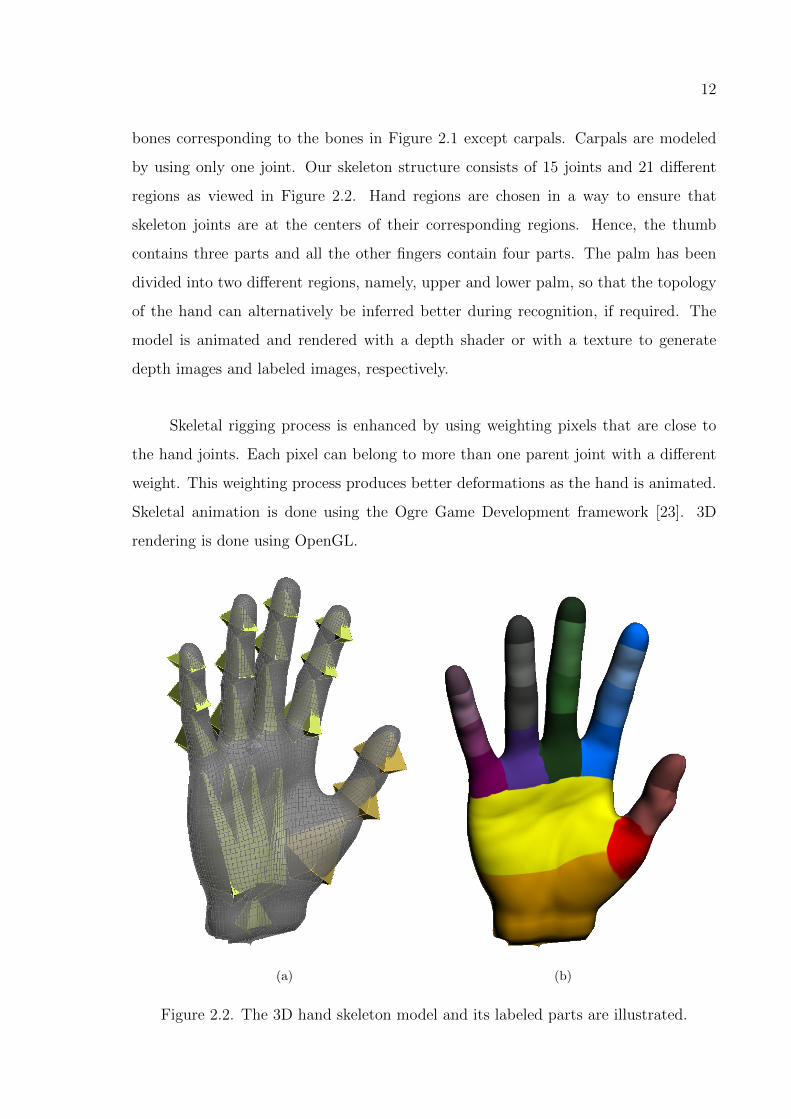
bones corresponding to the bones in Figure 2.1 except carpals. Carpals are modeled
by using only one joint. Our skeleton structure consists of 15 joints and 21 different
regions as viewed in Figure 2.2. Hand regions are chosen in a way to ensure that
skeleton joints are at the centers of their corresponding regions. Hence, the thumb
contains three parts and all the other fingers contain four parts. The palm has been
divided into two different regions, namely, upper and lower palm, so that the topology
of the hand can alternatively be inferred better during recognition, if required. The
model is animated and rendered with a depth shader or with a texture to generate
depth images and labeled images, respectively.
Skeletal rigging process is enhanced by using weighting pixels that are close to
the hand joints. Each pixel can belong to more than one parent joint with a different
weight. This weighting process produces better deformations as the hand is animated.
Skeletal animation is done using the Ogre Game Development framework [23]. 3D
rendering is done using OpenGL.
(a) (b)
Figure 2.2. The 3D hand skeleton model and its labeled parts are illustrated.

13
2.3. Customization for Different Hands
The framework normally uses a single skeleton rigged hand mesh. Although this
work concentrates on a single hand shape, the hand model is parameterized so that
the length of the fingers, size of the palm, etc., can be easily modified. The model is
easily customizable for different variations of the human hand.
Synthesized data generation details are discussed in Section 6.3. Generated im-
ages and animated skeleton joint coordinates are used as ground truth during training.
14
3. BACKGROUND
In this chapter, we review the techniques that are used in articulated pose model-
ing, pose configuration estimation, and dynamic gesture tracking both for human body
and human hand. We speak briefly about the sensors and how new sensors contributed
to developing faster and affordable algorithms.
Hand gestures are a natural part of human interaction. In addition to their com-
plementary roles in speech based interaction, they play a primary role when speech
is absent, as in sign language based interaction. Attempts to use the hand gesture
modality in human computer interaction (HCI) has intensified research efforts for ar-
ticulated hand pose tracking and hand shape recognition in the last decade. Hand
gesture tracking meant to track the centroid of the hand and capture dynamic gestures
in time. However most of the information passed during a sign language interaction is
gathered from the pose configuration of the hand. High degree of articulation poses a
challenging task for capturing the exact pose of the hand in a fast manner.
Recent advances have been made on the depth camera front. Achievements in the
field of high-speed depth sensors has greatly facilitated the image processing and seg-
mentation part of the task. Usually, time-of-flight depth cameras were used to acquire
depth (range) images. Two developments have recently accelerated implementations
of HCI using human body and hand gestures: The first is the release and widespread
acceptance of the Kinect [2] depth sensor. With its ability to generate depth images
independent of external illumination conditions, this sensor makes the human body
and hand detection and segmentation a simple task. The second development is the
emergence of fast discriminative approaches using simple depth features coupled with
GPU implementation; enabling real-time human body pose extraction [3, 24].
The last decade witnessed the step by step attack to the real-time pose estima-
tion problem both for human body and human hand. Some of the roots of the pose
estimation problem comes from object classification. Classification of smaller parts of
15
an object can be combined into a bigger agenda as presented by Fergus et al. [25].
They capture scale invariant features from a dataset in an unsupervised fashion. They
then utilize these constellation of small object parts for object classification. Winn et
al. [26] use conditional random fields in a similar fashion for detecting partially oc-
cluded objects. Liu et al. [27] use time-of-flight cameras to acquire depth images for
hand gesture recognition. Their hand detection method is based on measuring the
shape similarity by thresholding the depth data and using Chamfer distance. They
recognize gestures using shape, location, trajectory, orientation and speed features of
the hand. Grest et al. [28] use non-linear optimization techniques to iteratively fit a
3D body model to depth images in near real-time. Knoop et al. [29] use sensor fusion
from different cues such as time-of-flight depth cameras, stereo cameras, and monoc-
ular images for capturing the human body pose by using a 3D model. Zhu et al. [30]
utilize depth images and tracking for labeling the upper body of a human. Body parts
classification is achieved by reducing the labeling problem to linear programming. In-
verse kinematics is also incorporated for better tracking. First the pixels are classified
as belonging to a body part, then the upper body pose is estimated. Bourdev et al. [31]
propose a two-layer supervised classification/regression model for detecting people and
localizing body components. The first layer consists of classifiers that specializes on
detecting local patterns in the image. The second layer combines the output of the
classifiers in a max-margin framework. Siddiqui et al. [32] use a data driven MCMC
approach to find an optimal pose based on a likelihood that compares synthesized
depth images to the observed depth image. They incorporate extra data from head
and torso estimators for fast convergence of their method. Plagemann et al. [33] con-
centrate on real-time localization of important body parts such as head, hands, and
feet in depth images. They both estimate the location and orientation of hands in a
probabilistic manner. Ganapathi et al. [34] use time-of-flight cameras for model based
tracking of human body using Bayesian networks. They coarsely find important body
part locations and use the noisy observations as input to their probabilistic tracking
framework. Suryanayaran et al. [35] use depth for dynamically recognizing scale and
rotation invariant poses. Using a volumetric shape descriptor formed by augmenting a
2D image, they classify six signature hand poses. Shotton et al. [3, 6] use classification
forests for human pose estimation using depth data. Doliotis et al. [36] train a shape
16
classifier from synthesized depth images and try to segment and recognize American
Sign Language shapes. In [37], Gallo et al. use depth images along with PCA and
Flusser moments for detection of predefined shape postures. Billiet et al. [38] extract
finger alignments after segmenting the hand, and use a rule-based approach for rep-
resenting hand poses. Some works make use of disparities to get depth information,
and some works use color and depth data together for estimating hand poses [39, 40].
Liang et al. [40] use a model based estimation framework which utilizes both the color
and depth cues for tracking fingertips. They then employ articulated ICP for tracking
the full hand pose.
The state-of-the-art approaches for human body pose estimation generally use the
Kinect [2] camera. They employ a variety of techniques: Shotton et al. [3] use a large
amount of labeled synthetic images to train a randomized decision forest (RDF) [41]
for the task or body part recognition. In a later study, Girschick et al. [24] use the same
methodology, but let each pixel vote for joint coordinates; and learn the voting weights
from data. Ye et al. [42] rely on pre–captured motion exemplars to estimate the body
configuration as well as the semantic labels of the point cloud. Lopez et al. [43] use
an upper body model and tracks it using a hierarchical particle filter. Although these
ideas may be extended to extracting the 3D pose of the hand, the problem is made
more difficult by the increased pose variability and self-occlusion.
There are also tracking based skeleton extraction methods in the literature. Most
skeleton tracking algorithms estimate a skeleton by exploiting kinematic constraints
and dynamics of the object: Bregler et al. [44] propose new linear update equations
of motion for tracking the walking videos of humans. They assume walking motion is
involving minimal acceleration and they model by a twist motion model. Their ini-
tialization is costly and all the remaining tracking purely depends on the initialization
step. Sigal et al. [45] use belief propagation over particle sets of body parts. They learn
conditional probabilities of body connections from motion captured training data. The
parts of body are sampled from a 3D articulated human model. Simple bottom–up
body part detectors are also implemented for automatic re-initialization and recovery
from tracking errors. They run their algorithm by using four calibrated color cameras
17
with successful results. Wang et al. [46] employ a nearest neighbor pose classification
from a sampled synthetic hand pose dataset. Their tracking framework depends on
using a color glove specially designed for easily recovering the hand regions from color
images. They then utilize inverse kinematic constraints for fine tuning the captured
pose. Brubaker et al. [47] use sequential Monte Carlo tracking with kinematic con-
straints for tracking walking motion in monocular video. These algorithms can achieve
high frame rates by using temporal domain information between frames. Unfortu-
nately, without constant re-initialization, these tracking algorithms are going to lose
track eventually.
There are several surveys on hand pose estimation and gesture recognition [48,
49]. Erol et al. [48] review hand pose estimation methods. They investigate both
partial and full pose estimation methods. They categorize the full pose estimation
methods into single frame and model-based tracking methods. Most of the works in
the literature focus on grayscale or color based methods. These works use either single
or multiple cameras. Athitsos et al. [50] create a large synthetic hand pose database
using an articulated model and estimate 3D hand pose from a single frame cluttered
image by finding the closest match. [51] recovers hand pose from a single frame using
an RVM-based learning method. In order to overcome the self-occlusion problem,
multiple views are combined. Oikonomidis et al. [1] use Particle Swarm Optimization
for solving the 3D hand pose recovery problem. [52] works on monocular videos for
3D hand pose estimation. They track hand poses using a generative model-based
method. Thippur et al. [53] use visual shape descriptors for describing the hand shape.
Hand pose estimation studies have initially relied on 2D models [48]. Although pose
variability and occlusion limit the success of 2D approaches, successful partial models
have been defined [54].
Stenger et al. [55] use a 27 DOF 3D hand model composed of quadrics. They
utilize fast projection of quadrics on a 2D screen and edge detection as the features for
observing the hand from color images. They successfully track the pose configuration
by using an unscented Kalman filter. Rosales et al.designed a Specialized Mapping
Architecture (SMA) where a regression based method is employed for mapping hand
18
silhouettes to pose configurations [56]. They rendered hands using commercial library
[57]. A stochastic learning method is used to capture the mappings from the synthe-
sized data. In testing time, they segment the hands from color images, and feed the
extracted silhouettes to the SMA architecture for estimating pose configuration. Mo et
al. [58] work on low-resolution depth images acquired from a laser-based camera. Their
algorithm requires manual initialization and uses basic sets of finger poses for interpo-
lating a hand pose. Malassiotis et al. [59] use depth images generated from synthetic
3D hand models. They rely on depth cameras for successful segmentation of hands.
They then recognize German Sign Language hand shapes from depth images.
These approaches have achieved good performances even in the presence of occlu-
sions and pose changes, though their time performances have limited their application
in real-time HCI applications. In a recent study, Oikonomidis et al. [1] present a solu-
tion that makes use of both depth and color images. They propose a generative single
hypothesis model-based pose estimation method. They use particle swarm optimiza-
tion for solving the 3D hand pose recovery problem, and report accurate and robust
tracking in near real–time (15 fps), with a GPU based implementation.
Our work [5] has adapted the method in [3] to hand pose estimation with suc-
cessful results. They further enhanced randomized decision forest based hand pose
estimation by using multiple layers of forests. Clustering the hand pose configurations
and training a specialized RDF for each different cluster yielded better results. They
also utilized an RDF for detecting the cluster of the depth image in inference [60]. A
similar approach is also used in [61], which detects the hands in the first layer and then
classifies hand shapes in the second layer. Method of Keskin et al. [62] classifies hand
shapes in the first layer and then estimates the hand pose in the second layer.
Recent emphasis on manifold based tracking is also producing attention. Man-
ifold extraction techniques have evolved in last two decades considerably. Machine
learning can often be visualized in three major categories. Firstly, a dataset is consid-
ered as inputs and outputs in supervised learning. Secondly, a required goal is bound
with a reward in reinforcement learning. And in unsupervised learning, the objective is
19
to extract the structure of the underlying dataset. In manifold extraction, an approach
to unsupervised learning, we represent the original data Y , in a lower dimensional
embedded space X. Probabilistic variables in the lower dimensional space are named
as latent variables. Mackay [63] proposed Density networks, and employed a multi-
layer perceptron (MLP) to provide mapping from latent space to the data space. A
prior distribution is placed over the latent-space and the latent-spaces posterior dis-
tribution is approximated by sampling. Bishop et al. [64] used a radial basis function
(RBF) network instead of an MLP for faster training times. This model later became
the generative topographic mapping (GTM) [65] where the latent-space was uniformly
sampled, and a mixture model was fitted via the expectation-maximization (EM) al-
gorithm. The latent space uniform grid layout is shared with the self organizing map
(SOM) of Kohonen et al. [66]. These methods represent the latent space as a grid,
however, point representations of the latent-space are useful because they allow for
non-linear models. Points are easier to map through the non-linear mapping to the
data-space. Standard statistical tools that rely on linear mappings, such as principal
component analysis (PCA) and factor analysis (FA) may not be able to reflect the
structure of the data in a low dimensional embedding. PCA seeks a lower dimensional
sub-space in which the variance of the data is maximized. For visualization purposed,
generally a 2D sub-space is sought. However, two dimensions may not be enough to
capture the variability in the data. Structure of the data is most probably not captured.
PCA also has a latent variable model representation shown by Tipping et al. [67]. It is
strongly related to Factor Analysis (FA). Other famous works that focused on forming
the proximity matrix include Isomap by Tenenbaum et al. [68], and usage of spectral
clustering in Shi et al. [69].
Reducing the pose space dimensionality is favorable since human activities are
often observed to be located on a low dimensional latent space [70, 71]. Manifold
tracking depends on three main steps. First, a mapping between original pose space
to manifold must be available. Second, a mapping from manifold to original space
must also be defined. Third, how tracking occurs within the manifold must be defined.
PCA is linear and not adequate since the mapping from original space to manifold
space is almost always non-linear. Locally Linear Embedding (LLE) or Isomap can
20
capture this non-linear embedding, but they are not invertible. Inverse mapping is more
important since the tracking is to be done in the manifold space. Gaussian Process
Latent Variable Models [72] and Locally Linear Coordination (LLC, [73]) provide the
inverse mapping. Sminchisescu et al. [74] extract the underlying manifold by using
spectral embedding, a type of Gaussian mixture model. Inverse mapping is provided
by the learned Radial Basis Functions, after which the tracking is done by a linear
dynamical model. Urtasun et al. [75] utilize a GPLVM to learn prior models for 3D
human tracking. GPLVMs are used easily in combination with gradient descent based
optimization schemes since they generate smooth mappings between manifold and pose
space. In later works [76, 77], a Gaussian Process Dynamical Model (GPDM) is learned
from training data, which also learns a latent space dynamic model. Work by Moon et
al. [78] has examined the contribution of dynamics in the human motion tracking.
Tian et al. [79] use a GPLVM for 2D pose estimation. Particle filtering is used, where
the particles are sampled in the latent manifold space. On the other hand, Li et al. [80]
use LLC for learning the mappings. Their mapping is designed in a way so that close
points in the latent space map to close poses in the original pose space. Therefore,
a simple dynamical model could be used. In more recent approaches, Ek et al. [81]
design a shared GPLVM model which describes a method for recovering 3D human
body pose from silhouettes. Method encapsulates both pose and silhouette features,
and is generative,which allows to model the ambiguities of a silhouette representation
in a principled way. A dynamical model is learned for overcoming the ambiguities
using temporal consistency. Lee et al. [82] model hand shape variations using 4D torus
manifolds. They estimate the camera view angles, pose configuration of the hand at
the same time using Particle Filters that run on the extracted manifold. Advantages
and disadvantages of various embedding techniques are illustrated in Table 3.1.
In this thesis, we are going to discuss the key approaches required for estimation
of hand joints both in a single image setup and temporal domain tracking without
a need for regular re-initialization. The basis of the methodologies that is going to
be developed for single image estimation depends on Randomized Decision Forests.
Tracking in the time domain makes use of low dimensional manifold learning.
21
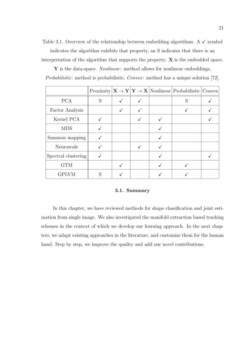
Table 3.1. Overview of the relationship between embedding algorithms. A X symbol
indicates the algorithm exhibits that property, an S indicates that there is an
interpretation of the algorithm that supports the property. X is the embedded space.
Y is the data-space. Nonlinear : method allows for nonlinear embeddings,
Probabilistic: method is probabilistic, Convex : method has a unique solution [72].
Proximity X→ Y Y→ X Nonlinear Probabilistic Convex
PCA S X X S X
Factor Analysis X X X X
Kernel PCA X X X X
MDS X X
Sammon mapping X X
Neuroscale X X X
Spectral clustering X X X
GTM X X X
GPLVM S X X X
3.1. Summary
In this chapter, we have reviewed methods for shape classification and joint esti-
mation from single image. We also investigated the manifold extraction based tracking
schemes in the context of which we develop our learning approach. In the next chap-
ters, we adapt existing approaches in the literature, and customize them for the human
hand. Step by step, we improve the quality and add our novel contributions.
22
4. SHAPE CLASSIFICATION FROM SINGLE DEPTH
IMAGE
The RDF model, which has been used for body pose estimation in [3] has been
adapted to a number of hand related tasks. One of our first attempts has been hand
shape classification [62]. In this chapter, we first present a shape classifier, which is an
adaptation of the RDF based pose estimation method of [3] to generic shapes. We call
this new type of RDF an RDF for shape classification (RDF-S).
The performance of the shape classification method is evaluated on real and
synthetic images, respectively. In particular, RDF-S is tested on the publicly available
ASL dataset of [83] and is shown to achieve a success rate of 97.8%. Multi-user ASL
letter recognition is a difficult task, and comparable good results to ours have been
reported in the literature on other datasets. [84] provides a good review of ASL letter
recognition on depth data.
4.1. Randomized Decision Forest (RDF)
A decision tree is used for inferring a set of posterior probabilities for the input. It
consists of internal nodes and leaf nodes; where the internal nodes propagate the data
to one of its children. In the binary case, decisions to split the data are simply yes/no
decisions. Leaf nodes do not make a decision but give statistical information about the
nature of the data. The type of statistical information depends on the application.
In randomized decision trees, the decisions on internal nodes are made by selecting
a random subset of the features. The aim is to reach leaf nodes that are as pure as
possible. A pure node consists of samples of only one class. Thus, the features are
selected to yield maximum information gain, in other words, minimum entropy. The
23
decision rule is usually of the form:
fn(v) < τn (4.1)
where fn(v) is a split function, v is the feature vector and τn is a threshold, at split
node n. A split function is a real valued function on a subset of features.
During training, the split functions and thresholds of nodes are chosen to satisfy
the minimum entropy condition. On the leaf nodes, statistics are collected using the
data associated with that node. In the case of classification, this is usually a histogram
of the class labels of the leaf node data.
Randomized Decision Forest (RDF) is an ensemble of decision trees. Each tree
can be trained on the same or slightly different datasets. During testing, the given
sample is processed in each tree separately. The statistics on the reached leaves are
combined for a common response. In classification problems, this is usually done by
accumulating normalized histograms in the leaves as shown by Shotton et al. [3]. Same
approach for estimating human body pose has been applied to estimation of human
hand pose [5].
4.2. Pixel Training and Classification using RDF (RDF-C)
During training, at each node of a randomized decision tree, a random subset of
features must be selected and a decision must be made using this subset. The training
data consists of large number of pixels of different depth images. Given a depth image
I, features are computed as
Fu,v(I,x) = I
(x +
u
I(x)
)− I
(x +
v
I(x)
)(4.2)
where u and v are offsets relative to the pixel position x, and they are normalized by
the depth at x, I(x). The node data consisting of (I,x) pairs are split into two sets
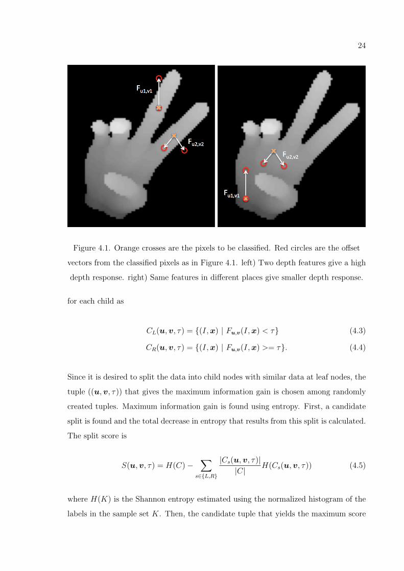
24
Figure 4.1. Orange crosses are the pixels to be classified. Red circles are the offset
vectors from the classified pixels as in Figure 4.1. left) Two depth features give a high
depth response. right) Same features in different places give smaller depth response.
for each child as
CL(u,v, τ) = {(I,x) | Fu,v(I,x) < τ} (4.3)
CR(u,v, τ) = {(I,x) | Fu,v(I,x) >= τ}. (4.4)
Since it is desired to split the data into child nodes with similar data at leaf nodes, the
tuple ((u,v, τ)) that gives the maximum information gain is chosen among randomly
created tuples. Maximum information gain is found using entropy. First, a candidate
split is found and the total decrease in entropy that results from this split is calculated.
The split score is
S(u,v, τ) = H(C)−∑
s∈{L,R}
|Cs(u,v, τ)||C|
H(Cs(u,v, τ)) (4.5)
where H(K) is the Shannon entropy estimated using the normalized histogram of the
labels in the sample set K. Then, the candidate tuple that yields the maximum score
25
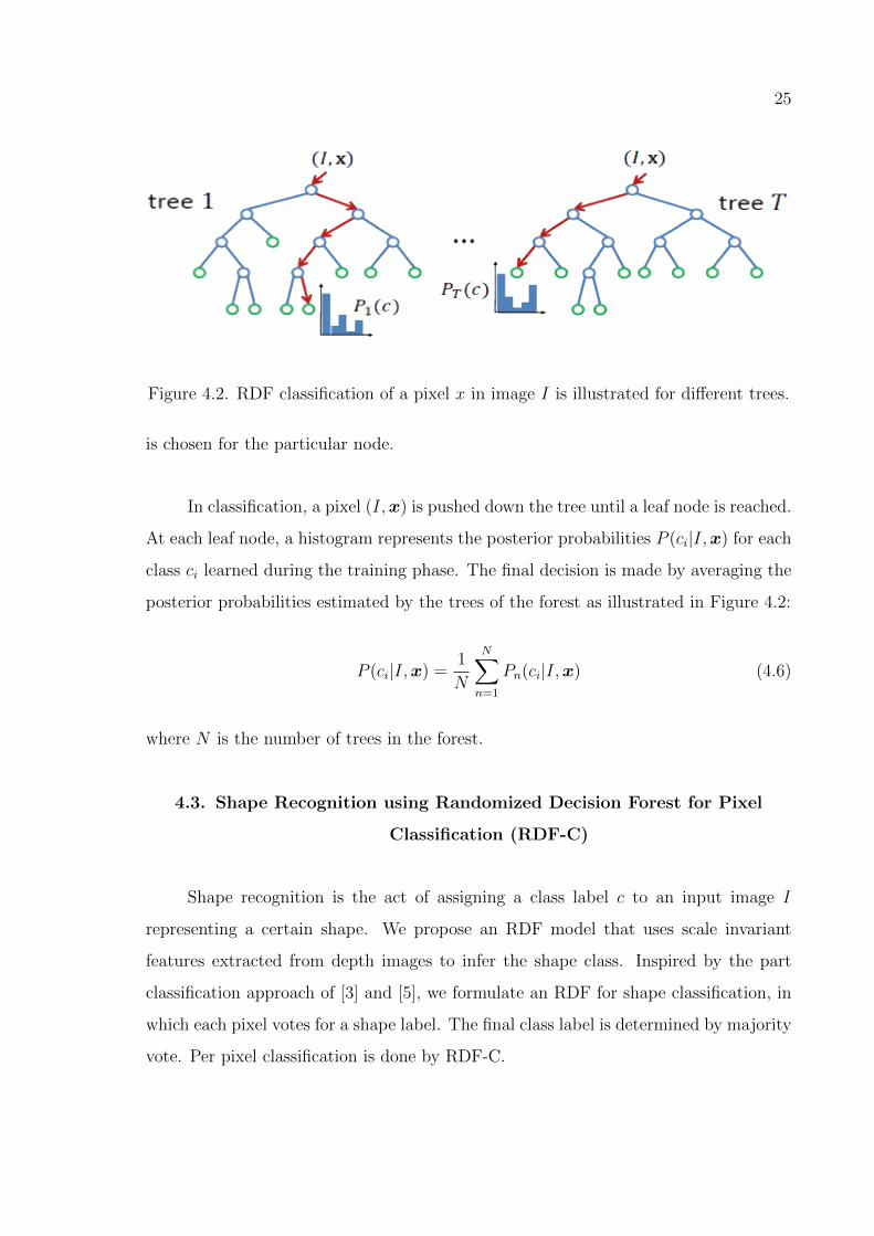
Figure 4.2. RDF classification of a pixel x in image I is illustrated for different trees.
is chosen for the particular node.
In classification, a pixel (I,x) is pushed down the tree until a leaf node is reached.
At each leaf node, a histogram represents the posterior probabilities P (ci|I,x) for each
class ci learned during the training phase. The final decision is made by averaging the
posterior probabilities estimated by the trees of the forest as illustrated in Figure 4.2:
P (ci|I,x) =1
N
N∑n=1
Pn(ci|I,x) (4.6)
where N is the number of trees in the forest.
4.3. Shape Recognition using Randomized Decision Forest for Pixel
Classification (RDF-C)
Shape recognition is the act of assigning a class label c to an input image I
representing a certain shape. We propose an RDF model that uses scale invariant
features extracted from depth images to infer the shape class. Inspired by the part
classification approach of [3] and [5], we formulate an RDF for shape classification, in
which each pixel votes for a shape label. The final class label is determined by majority
vote. Per pixel classification is done by RDF-C.
26
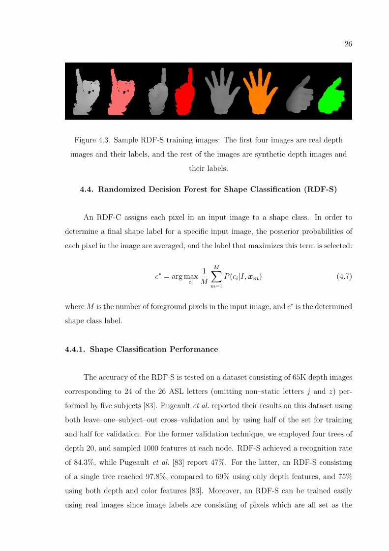
Figure 4.3. Sample RDF-S training images: The first four images are real depth
images and their labels, and the rest of the images are synthetic depth images and
their labels.
4.4. Randomized Decision Forest for Shape Classification (RDF-S)
An RDF-C assigns each pixel in an input image to a shape class. In order to
determine a final shape label for a specific input image, the posterior probabilities of
each pixel in the image are averaged, and the label that maximizes this term is selected:
c∗ = arg maxci
1
M
M∑m=1
P (ci|I,xm) (4.7)
where M is the number of foreground pixels in the input image, and c∗ is the determined
shape class label.
4.4.1. Shape Classification Performance
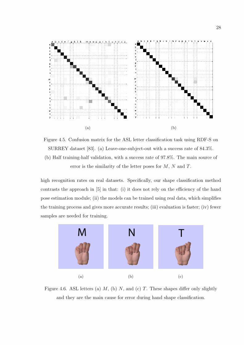
The accuracy of the RDF-S is tested on a dataset consisting of 65K depth images
corresponding to 24 of the 26 ASL letters (omitting non–static letters j and z) per-
formed by five subjects [83]. Pugeault et al. reported their results on this dataset using
both leave–one–subject–out cross–validation and by using half of the set for training
and half for validation. For the former validation technique, we employed four trees of
depth 20, and sampled 1000 features at each node. RDF-S achieved a recognition rate
of 84.3%, while Pugeault et al. [83] report 47%. For the latter, an RDF-S consisting
of a single tree reached 97.8%, compared to 69% using only depth features, and 75%
using both depth and color features [83]. Moreover, an RDF-S can be trained easily
using real images since image labels are consisting of pixels which are all set as the
27
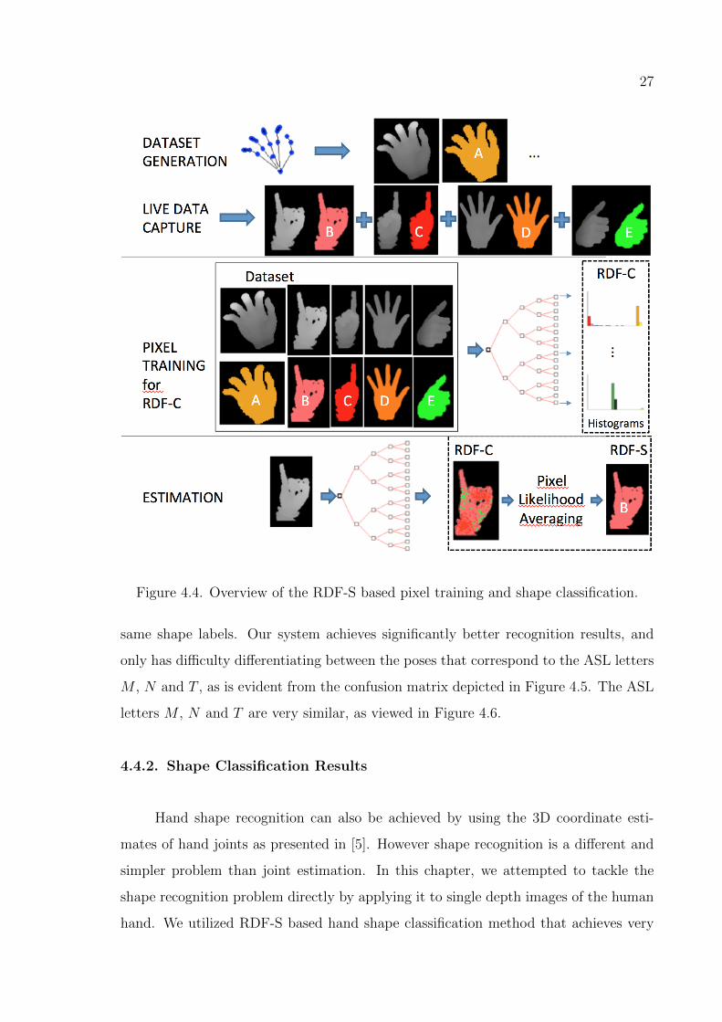
Figure 4.4. Overview of the RDF-S based pixel training and shape classification.
same shape labels. Our system achieves significantly better recognition results, and
only has difficulty differentiating between the poses that correspond to the ASL letters
M , N and T , as is evident from the confusion matrix depicted in Figure 4.5. The ASL
letters M , N and T are very similar, as viewed in Figure 4.6.
4.4.2. Shape Classification Results
Hand shape recognition can also be achieved by using the 3D coordinate esti-
mates of hand joints as presented in [5]. However shape recognition is a different and
simpler problem than joint estimation. In this chapter, we attempted to tackle the
shape recognition problem directly by applying it to single depth images of the human
hand. We utilized RDF-S based hand shape classification method that achieves very
28
(a) (b)
Figure 4.5. Confusion matrix for the ASL letter classification task using RDF-S on
SURREY dataset [83]. (a) Leave-one-subject-out with a success rate of 84.3%.
(b) Half training-half validation, with a success rate of 97.8%. The main source of
error is the similarity of the letter poses for M , N and T .
high recognition rates on real datasets. Specifically, our shape classification method
contrasts the approach in [5] in that: (i) it does not rely on the efficiency of the hand
pose estimation module; (ii) the models can be trained using real data, which simplifies
the training process and gives more accurate results; (iii) evaluation is faster; (iv) fewer
samples are needed for training.
(a) (b) (c)
Figure 4.6. ASL letters (a) M , (b) N , and (c) T . These shapes differ only slightly
and they are the main cause for error during hand shape classification.
29
5. HAND POSE ESTIMATION FROM SINGLE DEPTH
IMAGE USING PIXEL CLASSIFICATION
In Chapter 4, we have described the use of RDFs for hand shape classification.
However, our main goal is articulated hand pose estimation. This chapter gives the
details of the hand pose estimation method which employs pixel classification that is
described in Section 4.1. Section 5.1 explain the use of random decision forests for
hand pose estimation based on classification (RDF-C). We then extend the idea of
shape recognition to recognizing hand parts, as published in [3, 33, 25, 26, 31].
5.1. Hand Pose Estimation using Randomized Decision Forest for
Classification (RDF-C)
Shotton et al. [3] used RDF-C for human body pose estimation. Keskin et al. [5]
adapted that method to the hand pose estimation problem. The aim of the method is
to find the formerly trained corresponding pixel regions closest to each joint. However,
since some classification errors are anticipated, it would be better to find the mode of
the pixel positions instead of the mean. For this purpose, first the training data pixels
are labeled to define the area around the joints. A decision forest is trained using this
data. On the leaves, histograms are calculated using the classes of the pixels. Training
and testing framework of an RDF with a sample human hand model is demonstrated
in Figure 5.1.
For a given depth image, the RDF-C algorithm yields posterior probabilities of
each pixel for each class after classification. The resulting probability surfaces are gen-
erally multi-modal. Thus, simple averaging is not a suitable operation. For overcoming
the high impact of misclassified pixels on the centroid of the pixel locations of the same
class, a method that is more robust to false positives than averaging, must be used.
In this situation, mode finding is preferred instead of averaging. A local mode finding
approach, such as mean shift, can be used. The posterior probabilities assigned to
30
each pixel are used to estimate the joint positions as in [5]. The mean shift local mode
finding algorithm [85] is used to estimate the mode of the probability density of each
class label.
Figure 5.1. Overview of the RDF-C based pixel training and joint estimation.
First, a Gaussian kernel centered on a random point on the probability image is
placed. Then, a weighted mean of the probability image under this Gaussian kernel is
calculated. Weight indicates the importance of the pixel and is an estimate of the area
the pixel covers. Weights are calculated as
wI,x,ci = P (ci|I,x)I(x)2. (5.1)
The newly calculated mean point is used as the starting point of the next iteration.
This is repeated until converging to a local maximum. For finding the global maximum,
the algorithm runs several times, each time starting at a different initial point and the
highest peak is selected. A sample convergence of mean shift algorithm is shown
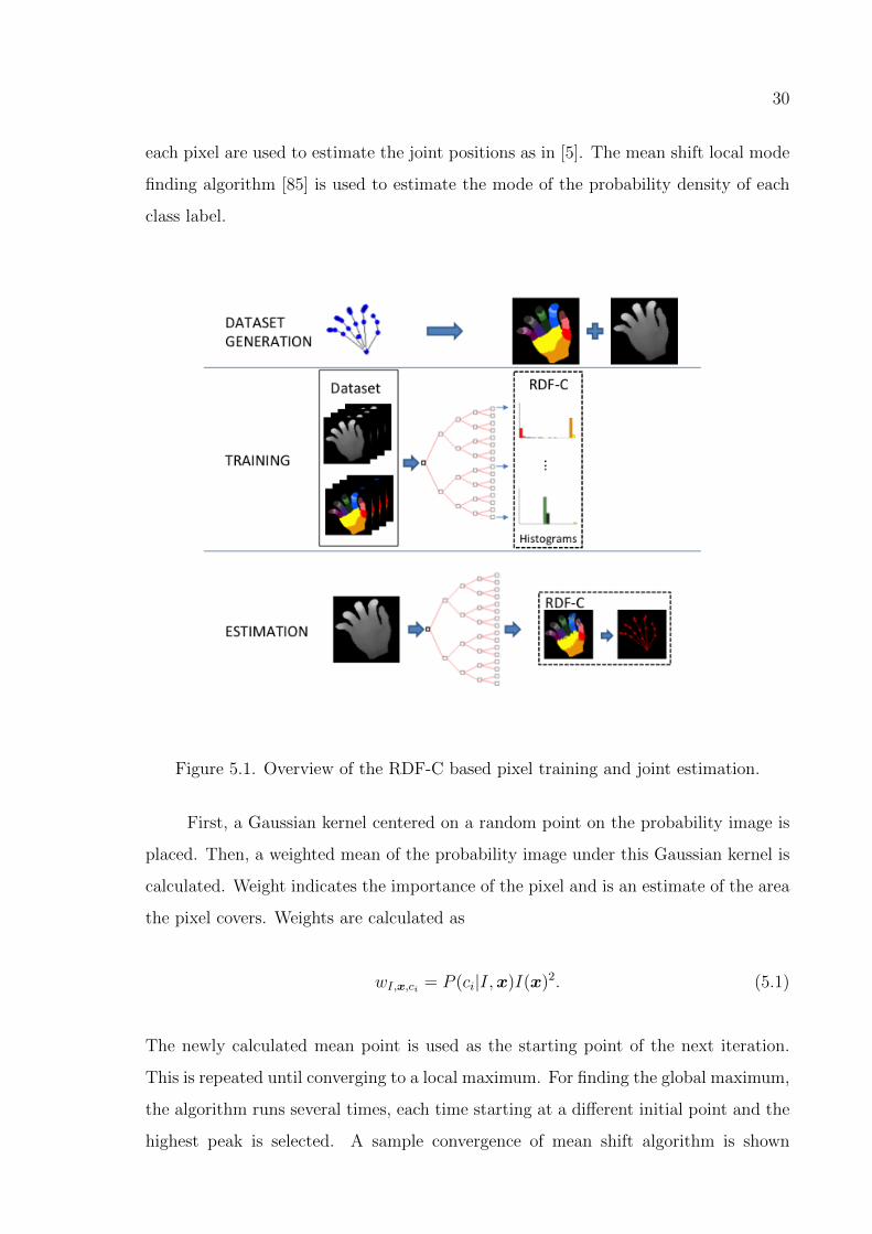
31
in Figure 5.2 for the first bone of the thumb finger. Each pixel in the classification
image evaluated by the RDF-C is normally represented by a probability distribution
of joints. Each pixel is painted by its maximum likelihood estimate in the figure for
facilitating the demonstration process. The bandwidth of each hand part is manually
selected based on the size of each hand part. Figure 5.3 shows the final skeletal output
found by the algorithm after each different hand region’s centroid is estimated using
mean shift. The depth of the found 2D coordinates of the joints are then approximated
by looking at the pixel’s corresponding depth value. Human hand’s thickness does not
vary much among its different joints. 3D position of the joint can be estimated by
shifting its depth coordinate with a certain amount of length into the scene.
5.2. Hand Pose Estimation from Single Depth Image using Hybrid
Classification Forests (RDF-H)
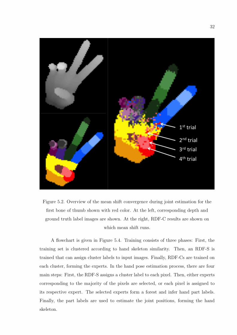
In this section, we propose a novel multi–layered hybrid approach to tackle the
complexity problem. The idea is to reduce the complexity of the model by dividing
the training set into smaller clusters, and to train RDF-Cs on each of these compact
sets. Thus, the RDF-Cs need to model only a small amount of variation, requiring
smaller memory. These experts accurately model a specific subset of the data, and infer
significantly better pose estimates. The main challenge is to direct the input towards
the correct experts, which can easily be done by training an RDF-S for detecting the
clusters.
We use RDF-S in designing a multi–layered hybrid RDF network to tackle the
articulated hand pose estimation problem. We divide the large dataset into simpler
sub–problems by clustering the dataset first. Then, each such cluster corresponds to a
hand shape that can be recognized with an RDF-S, and a separate hand pose estimator
is trained on each cluster, forming skeleton experts. A similar approach is used in [61],
which detects the hands in the first layer and then classifies hand shapes in the second
layer. Our method classifies hand shapes in the first layer and then estimates the hand
pose in the second layer.
32
Figure 5.2. Overview of the mean shift convergence during joint estimation for the
first bone of thumb shown with red color. At the left, corresponding depth and
ground truth label images are shown. At the right, RDF-C results are shown on
which mean shift runs.
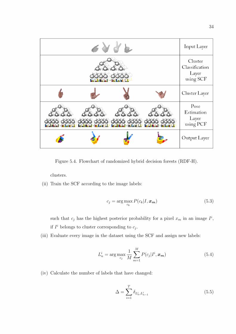
A flowchart is given in Figure 5.4. Training consists of three phases: First, the
training set is clustered according to hand skeleton similarity. Then, an RDF-S is
trained that can assign cluster labels to input images. Finally, RDF-Cs are trained on
each cluster, forming the experts. In the hand pose estimation process, there are four
main steps: First, the RDF-S assigns a cluster label to each pixel. Then, either experts
corresponding to the majority of the pixels are selected, or each pixel is assigned to
its respective expert. The selected experts form a forest and infer hand part labels.
Finally, the part labels are used to estimate the joint positions, forming the hand
skeleton.
33
(a) (b) (c) (d)
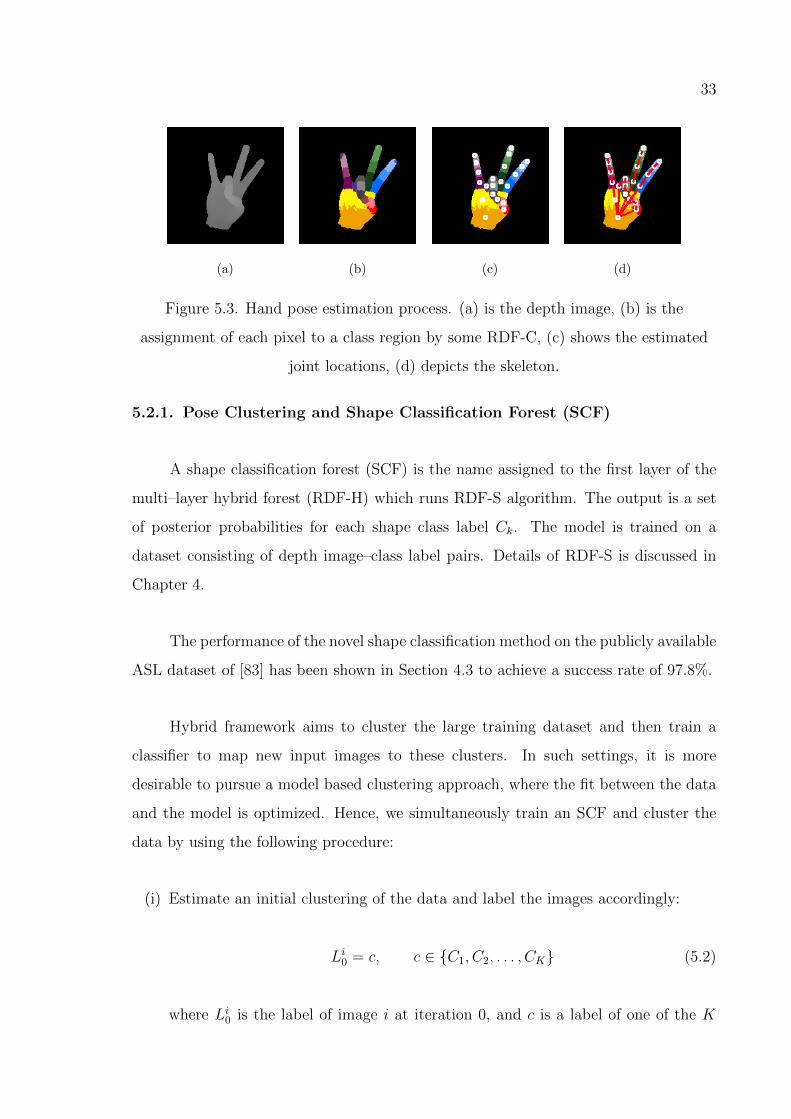
Figure 5.3. Hand pose estimation process. (a) is the depth image, (b) is the
assignment of each pixel to a class region by some RDF-C, (c) shows the estimated
joint locations, (d) depicts the skeleton.
5.2.1. Pose Clustering and Shape Classification Forest (SCF)
A shape classification forest (SCF) is the name assigned to the first layer of the
multi–layer hybrid forest (RDF-H) which runs RDF-S algorithm. The output is a set
of posterior probabilities for each shape class label Ck. The model is trained on a
dataset consisting of depth image–class label pairs. Details of RDF-S is discussed in
Chapter 4.
The performance of the novel shape classification method on the publicly available
ASL dataset of [83] has been shown in Section 4.3 to achieve a success rate of 97.8%.
Hybrid framework aims to cluster the large training dataset and then train a
classifier to map new input images to these clusters. In such settings, it is more
desirable to pursue a model based clustering approach, where the fit between the data
and the model is optimized. Hence, we simultaneously train an SCF and cluster the
data by using the following procedure:
(i) Estimate an initial clustering of the data and label the images accordingly:
Li0 = c, c ∈ {C1, C2, . . . , CK} (5.2)
where Li0 is the label of image i at iteration 0, and c is a label of one of the K
34
Figure 5.4. Flowchart of randomized hybrid decision forests (RDF-H).
clusters.
(ii) Train the SCF according to the image labels:
cj = arg maxck
P (ck|I,xm) (5.3)
such that cj has the highest posterior probability for a pixel xm in an image I i,
if I i belongs to cluster corresponding to cj.
(iii) Evaluate every image in the dataset using the SCF and assign new labels:
Lin = arg max
cj
1
M
M∑m=1
P (cj|I i,xm) (5.4)
(iv) Calculate the number of labels that have changed:
∆ =T∑i=1
δLin,Lin−1(5.5)
35
where δ is the Kronecker delta and T is the number of images in the dataset.
(v) If ∆ > 0, go to Step 2. Otherwise, return.
This method iteratively estimates new clusters and models them until the model
and the clusters fit and no label changes in an iteration. To supply the algorithm with
initial clusters, we apply spectral clustering. Spectral clustering methods are based
on the Min–Cut algorithm, which partitions graph nodes by minimizing a certain cost
associated with each edge in the graph [86]. This is a binary clustering method, which
can be used to hierarchically cluster data into multiple clusters. We use a related
algorithm that has been proposed by Meila et al. [87], which can estimate multiple
clusters. In this method, a similarity matrix is formed for the samples to be clustered,
where each entry Sij in the matrix corresponds to the similarity of samples i and j. As
the similarity measure, the reciprocal of a distance measure can be used.
The distance between two skeletal configurations is taken to be the weighted sum
of the absolute differences of each angle pair. Using the pairwise distances of each
configuration, we can estimate a clustering as follows:
Dij = ||W(vi − vj)||1 (5.6)
α = max (D) (5.7)
Sij = 1− 1
αDij (5.8)
Rii =∑j
Sij (5.9)
P = SR−1 (5.10)
Here, vi and vj are the vectors formed by all the angles of a skeleton. W is a diagonal
matrix, such that Wii is the weight of the angle i. α is the maximum amount of distance
recorded in D. S is the similarity matrix formed by normalizing the distance matrix
D according to α and subtracting each element from 1. Then, each column ci of S is
normalized using the sum of elements in row ri to form the matrix P. We find the
eigenvectors corresponding to the m largest eigenvalues of this matrix in the form of
a N ×m matrix. Each row of this matrix is a m dimensional representative of one of
36
the N samples. The rows of this matrix are clustered using the conventional k–means
method.
5.2.2. Pose Estimation with Pose Classification Forests (PCF)
We compare the success of the RDF-H with the results in [5]. Whereas the method
of [5] achieves a per pixel classification rate of 68.0% on a large synthetic dataset, the
multi–layered method achieves a classification rate of 91.2%.
5.2.3. Pose Estimation Using a Hybrid RDF Network (RDF-H)
First, we simultaneously train an SCF (Φ) and cluster a dataset D into K clusters
Dk, k = 1, . . . , K, using the method of Section 5.2.1. Next, we train K PCFs, depicted
as Ψk, on the clusters Dk.
Upon encountering a new input depth image, Φ classifies the image into one of the
K clusters using by assigning a label Ci to it, using the method in Section 4.4. Instead
of assigning a hard label, we take labels that correspond to the largest three of the
average posterior probabilities ρj = 1M
∑Mm=1 P (cj|I,xm). Without loss of generality,
we call these labels C1, C2 and C3 with posterior probabilities ρ1, ρ2 and ρ3. The
weighted sum of the hand part posteriors as estimated by the corresponding PCFs
Ψ1, Ψ2 and Ψ3 is taken to be the final posterior probability for each pixel, where the
weights are ρ1, ρ2 and ρ3:
P (cj|I,x) =3∑
i=1
ρiP (cj|I,x,Ψi) (5.11)
Finally, these posterior probabilities estimated by a collection of forests are used to
estimate the hand pose as explained in Section 5.2.2.
The SCF assigns a cluster label to each pixel in an input image. This information
can be used in two different ways: (i) a pose label for the entire image can be estimated
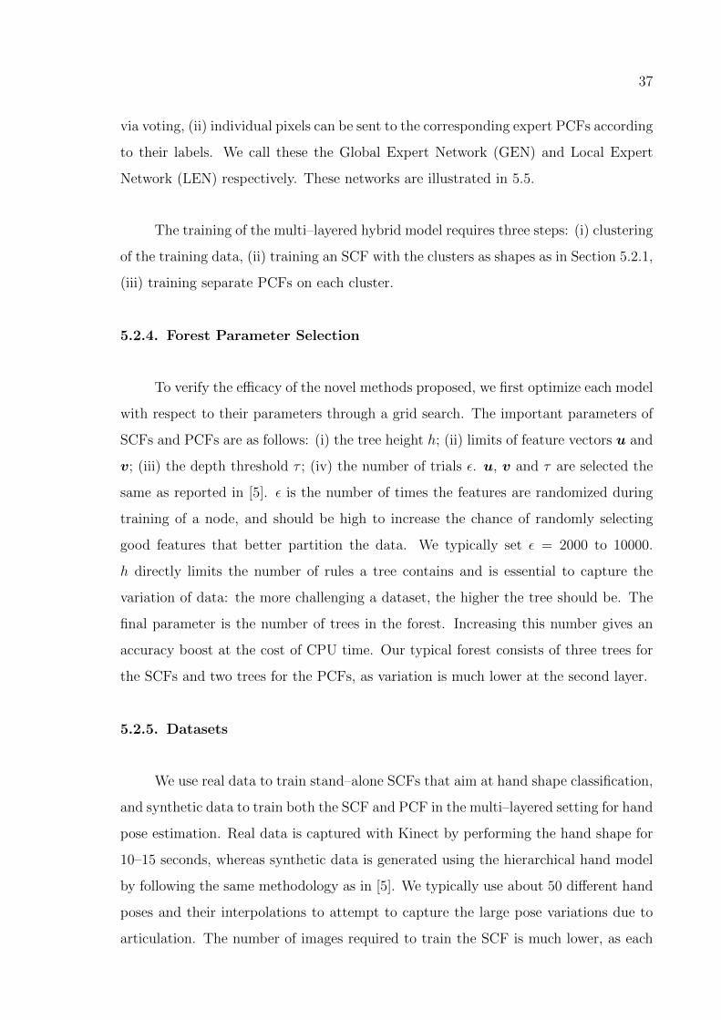
37
via voting, (ii) individual pixels can be sent to the corresponding expert PCFs according
to their labels. We call these the Global Expert Network (GEN) and Local Expert
Network (LEN) respectively. These networks are illustrated in 5.5.
The training of the multi–layered hybrid model requires three steps: (i) clustering
of the training data, (ii) training an SCF with the clusters as shapes as in Section 5.2.1,
(iii) training separate PCFs on each cluster.
5.2.4. Forest Parameter Selection
To verify the efficacy of the novel methods proposed, we first optimize each model
with respect to their parameters through a grid search. The important parameters of
SCFs and PCFs are as follows: (i) the tree height h; (ii) limits of feature vectors u and
v; (iii) the depth threshold τ ; (iv) the number of trials ε. u, v and τ are selected the
same as reported in [5]. ε is the number of times the features are randomized during
training of a node, and should be high to increase the chance of randomly selecting
good features that better partition the data. We typically set ε = 2000 to 10000.
h directly limits the number of rules a tree contains and is essential to capture the
variation of data: the more challenging a dataset, the higher the tree should be. The
final parameter is the number of trees in the forest. Increasing this number gives an
accuracy boost at the cost of CPU time. Our typical forest consists of three trees for
the SCFs and two trees for the PCFs, as variation is much lower at the second layer.
5.2.5. Datasets
We use real data to train stand–alone SCFs that aim at hand shape classification,
and synthetic data to train both the SCF and PCF in the multi–layered setting for hand
pose estimation. Real data is captured with Kinect by performing the hand shape for
10–15 seconds, whereas synthetic data is generated using the hierarchical hand model
by following the same methodology as in [5]. We typically use about 50 different hand
poses and their interpolations to attempt to capture the large pose variations due to
articulation. The number of images required to train the SCF is much lower, as each
38
(a)
(b)
Figure 5.5. Different types of hybrid RDF networks. Φ depicts the SCF, and Ψi
depicts the expert PCF corresponding to the cluster Ci. (a) Global Expert Network:
The experts are selected according to the pose label. (b) Local Expert Network: Each
pixel is sent to its own expert.
39
class label receives sufficiently many pixels. This contrasts the problem of small size of
finger tips for PCFs.
5.2.6. Shape Classification Performance
Shape classification layer is already trained and tested in Section 4.4.1. We use
directly the results of RDF-S as the first layer of our RDF-H.
5.2.7. Hand Pose Estimation
Two new factors introduced by the hybrid framework are the number of clustersK
and the diagonal matrix W used in estimating the pairwise distances of two skeletons.
Increasing K reduces the complexity of the PCFs in the second layer, while increasing
that of the SCF in the primary layer. On the other hand, the individual elements
of the weight matrix W determine the type of variation a cluster will contain: if
we penalize the global rotation angles with large weights, pose clusters will contain
variations in fingers mostly. Likewise, giving lower weights to the global rotation angles
causes the clusters to contain more camera view point changes. By conducting several
experiments, we determined that global rotation is the type of variation that is harder
to capture by PCFs, mainly due to the rotation variant features used in the training
phase. Therefore, we penalize the global angles with larger weights. We gradually
decrease the weights from the palm to the fingers, allowing the finger tips to move
rather freely.
Moreover, we proposed two different flavors of information passing from the first
layer to the second layer, namely GEN and LEN. A preliminary test is devised for
choosing between GEN and LEN. Per pixel classification rates are given in Table 5.1.
Previously implemented model in the literature from [5] achieves a success rate of 68.0%
on this dataset, whereas GEN achieves 91.2% and LEN achieves 90.9%. As expected,
the expert networks perform significantly better. On the other hand, the difference
between GEN and LEN is negligible in this case. Since LEN uses a different tree for
each different pixel, its runtime performance is slower. For the sake of less complexity,
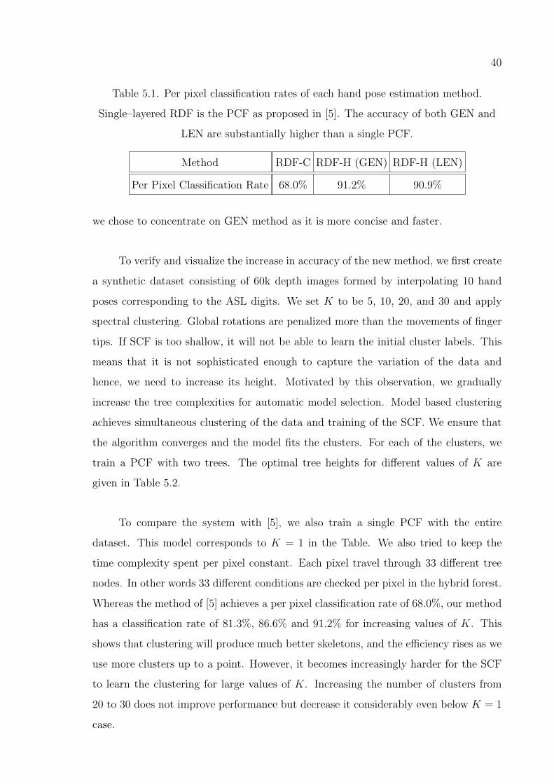
40
Table 5.1. Per pixel classification rates of each hand pose estimation method.
Single–layered RDF is the PCF as proposed in [5]. The accuracy of both GEN and
LEN are substantially higher than a single PCF.
Method RDF-C RDF-H (GEN) RDF-H (LEN)
Per Pixel Classification Rate 68.0% 91.2% 90.9%
we chose to concentrate on GEN method as it is more concise and faster.
To verify and visualize the increase in accuracy of the new method, we first create
a synthetic dataset consisting of 60k depth images formed by interpolating 10 hand
poses corresponding to the ASL digits. We set K to be 5, 10, 20, and 30 and apply
spectral clustering. Global rotations are penalized more than the movements of finger
tips. If SCF is too shallow, it will not be able to learn the initial cluster labels. This
means that it is not sophisticated enough to capture the variation of the data and
hence, we need to increase its height. Motivated by this observation, we gradually
increase the tree complexities for automatic model selection. Model based clustering
achieves simultaneous clustering of the data and training of the SCF. We ensure that
the algorithm converges and the model fits the clusters. For each of the clusters, we
train a PCF with two trees. The optimal tree heights for different values of K are
given in Table 5.2.
To compare the system with [5], we also train a single PCF with the entire
dataset. This model corresponds to K = 1 in the Table. We also tried to keep the
time complexity spent per pixel constant. Each pixel travel through 33 different tree
nodes. In other words 33 different conditions are checked per pixel in the hybrid forest.
Whereas the method of [5] achieves a per pixel classification rate of 68.0%, our method
has a classification rate of 81.3%, 86.6% and 91.2% for increasing values of K. This
shows that clustering will produce much better skeletons, and the efficiency rises as we
use more clusters up to a point. However, it becomes increasingly harder for the SCF
to learn the clustering for large values of K. Increasing the number of clusters from
20 to 30 does not improve performance but decrease it considerably even below K = 1
case.
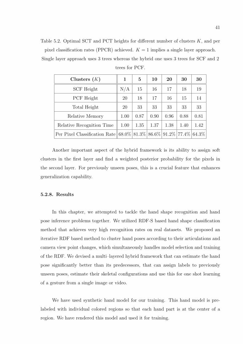
41
Table 5.2. Optimal SCT and PCT heights for different number of clusters K, and per
pixel classification rates (PPCR) achieved. K = 1 implies a single layer approach.
Single layer approach uses 3 trees whereas the hybrid one uses 3 trees for SCF and 2
trees for PCF.
Clusters (K) 1 5 10 20 30 30
SCF Height N/A 15 16 17 18 19
PCF Height 20 18 17 16 15 14
Total Height 20 33 33 33 33 33
Relative Memory 1.00 0.87 0.90 0.96 0.88 0.81
Relative Recognition Time 1.00 1.35 1.37 1.38 1.40 1.42
Per Pixel Classification Rate 68.0% 81.3% 86.6% 91.2% 77.4% 64.3%
Another important aspect of the hybrid framework is its ability to assign soft
clusters in the first layer and find a weighted posterior probability for the pixels in
the second layer. For previously unseen poses, this is a crucial feature that enhances
generalization capability.
5.2.8. Results
In this chapter, we attempted to tackle the hand shape recognition and hand
pose inference problems together. We utilized RDF-S based hand shape classification
method that achieves very high recognition rates on real datasets. We proposed an
iterative RDF based method to cluster hand poses according to their articulations and
camera view point changes, which simultaneously handles model selection and training
of the RDF. We devised a multi–layered hybrid framework that can estimate the hand
pose significantly better than its predecessors, that can assign labels to previously
unseen poses, estimate their skeletal configurations and use this for one shot learning
of a gesture from a single image or video.
We have used synthetic hand model for our training. This hand model is pre-
labeled with individual colored regions so that each hand part is at the center of a
region. We have rendered this model and used it for training.
42
Specifically, our shape classification method contrasts the approach in our previ-
ous work [5] such that: (i) it does not rely on the efficiency of the hand pose estimation
module; (ii) the models can be trained using real data, which simplifies the training
process and gives more accurate results; (iii) evaluation is faster; iv) fewer samples are
needed for training.
Furthermore, hybrid framework solves the problem of large memory requirements
and manages to capture the large pose and camera view point variations of the hand.
Hybrid hand pose estimation framework uses a novel model based clustering technique
that simultaneously clusters the data and trains the SCF to assign cluster labels to
data. For each cluster, we train a separate PCF that learns to assign pixels to hand
part labels. As the training set is much smaller for clusters, training is much faster,
the PCTs formed are shallower, and the per pixel classification accuracy of the PCFs
is higher.
We focused on optimizing the speed and pixel classification accuracy of the sys-
tem, in particular by performing grid search over all model parameters. The resulting
framework is capable of retrieving images from the depth camera [2], apply per pixel
classification using the multi–layered hybrid RDFs, estimate the joint locations from
several hypotheses in the mean shift phase, and finally use these locations for pose
classification at 30 fps, which is the limit of the depth camera.
Achieving a higher per pixel classification rate also improves the performance of
mean shift algorithm. This also improves the quality of the pose estimation. More
detailed analysis about the effects of pixel classification quality on estimated joints will
be discussed in Chapter 6.
The novel shape classification and 3D hand pose estimation methods introduced
in this paper significantly improve the performance of hand shape recognition and
hand pose estimation tasks, and are general enough to be applied to other generic
shape recognition or body pose estimation problems.
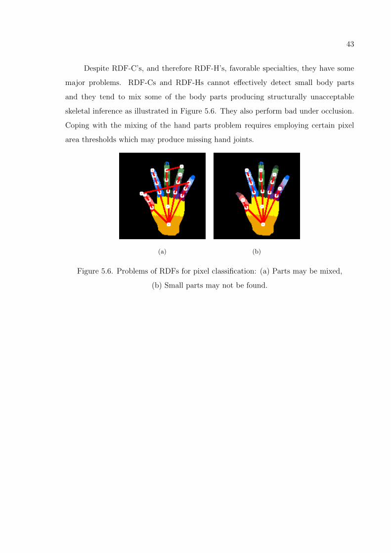
43
Despite RDF-C’s, and therefore RDF-H’s, favorable specialties, they have some
major problems. RDF-Cs and RDF-Hs cannot effectively detect small body parts
and they tend to mix some of the body parts producing structurally unacceptable
skeletal inference as illustrated in Figure 5.6. They also perform bad under occlusion.
Coping with the mixing of the hand parts problem requires employing certain pixel
area thresholds which may produce missing hand joints.
(a) (b)
Figure 5.6. Problems of RDFs for pixel classification: (a) Parts may be mixed,
(b) Small parts may not be found.
44
6. HAND POSE ESTIMATION WITH REGRESSION
BASED METHODS
In this chapter, we will integrate the methods that we introduced in previous
chapters to build a better joint estimator. RDF-S, RDF-C, and RDF-H all rely on
pixel classification. In the case of human hand, this transient pixel classification phase
comes with a big disadvantage. The human hand is a highly deformable and self-
occluding limb. Therefore, pixel classification based joint estimation is prone to the
occlusion problem. If the regions of the hand is not seen in the captured depth image
then there is no easy way to predict the unseen joints. In this chapter, we will develop
a regression based randomized forest for skipping the pixel classification phase. The
resulting joint estimator will therefore be robust against self-occlusion. In addition to
that, we will also incorporate the hierarchical structure of the human hand into joint
pose estimation methodology, instead of estimating all the joints independently.
In Section 6.1, we implement a regression based approach. Then we introduce
hierarchical constraints of the hand into consideration for further improving the perfor-
mance of this method as illustrated in Section 6.2. We then compare the performances
of all the methods we introduced so far. In Section 6.3, we give the details of the hand
data generation step and introduce the datasets that we use. Section 6.4 discusses the
fine-tuning of the essential training parameters, namely the forest size, the tree depth,
the probe distance, the depth threshold, and the mean shift bandwidth. In Section 6.5,
the fine-tuned RDFs are tested on four different datasets. We first test on the train-
ing dataset to gather information about the characteristics of the methods, and then
extend our tests to two different synthetic and one real test datasets.
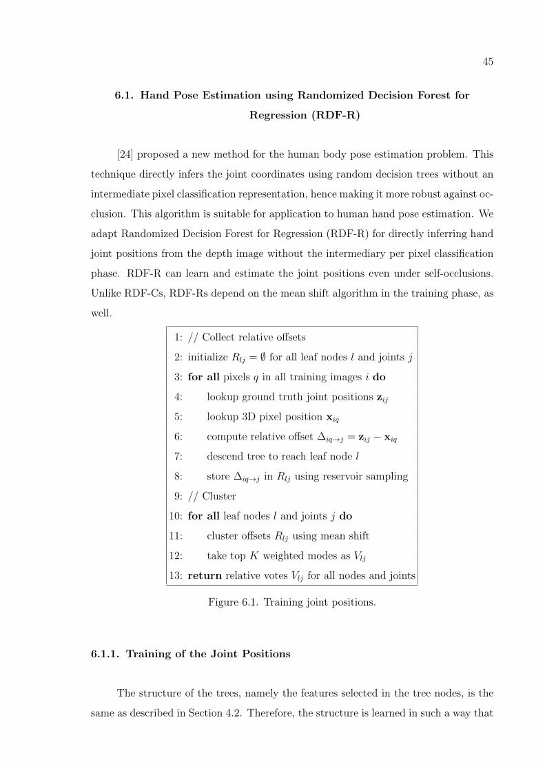
45
6.1. Hand Pose Estimation using Randomized Decision Forest for
Regression (RDF-R)
[24] proposed a new method for the human body pose estimation problem. This
technique directly infers the joint coordinates using random decision trees without an
intermediate pixel classification representation, hence making it more robust against oc-
clusion. This algorithm is suitable for application to human hand pose estimation. We
adapt Randomized Decision Forest for Regression (RDF-R) for directly inferring hand
joint positions from the depth image without the intermediary per pixel classification
phase. RDF-R can learn and estimate the joint positions even under self-occlusions.
Unlike RDF-Cs, RDF-Rs depend on the mean shift algorithm in the training phase, as
well.
1: // Collect relative offsets
2: initialize Rlj = ∅ for all leaf nodes l and joints j
3: for all pixels q in all training images i do
4: lookup ground truth joint positions zij
5: lookup 3D pixel position xiq
6: compute relative offset ∆iq→j = zij − xiq
7: descend tree to reach leaf node l
8: store ∆iq→j in Rlj using reservoir sampling
9: // Cluster
10: for all leaf nodes l and joints j do
11: cluster offsets Rlj using mean shift
12: take top K weighted modes as Vlj
13: return relative votes Vlj for all nodes and joints
Figure 6.1. Training joint positions.
6.1.1. Training of the Joint Positions
The structure of the trees, namely the features selected in the tree nodes, is the
same as described in Section 4.2. Therefore, the structure is learned in such a way that
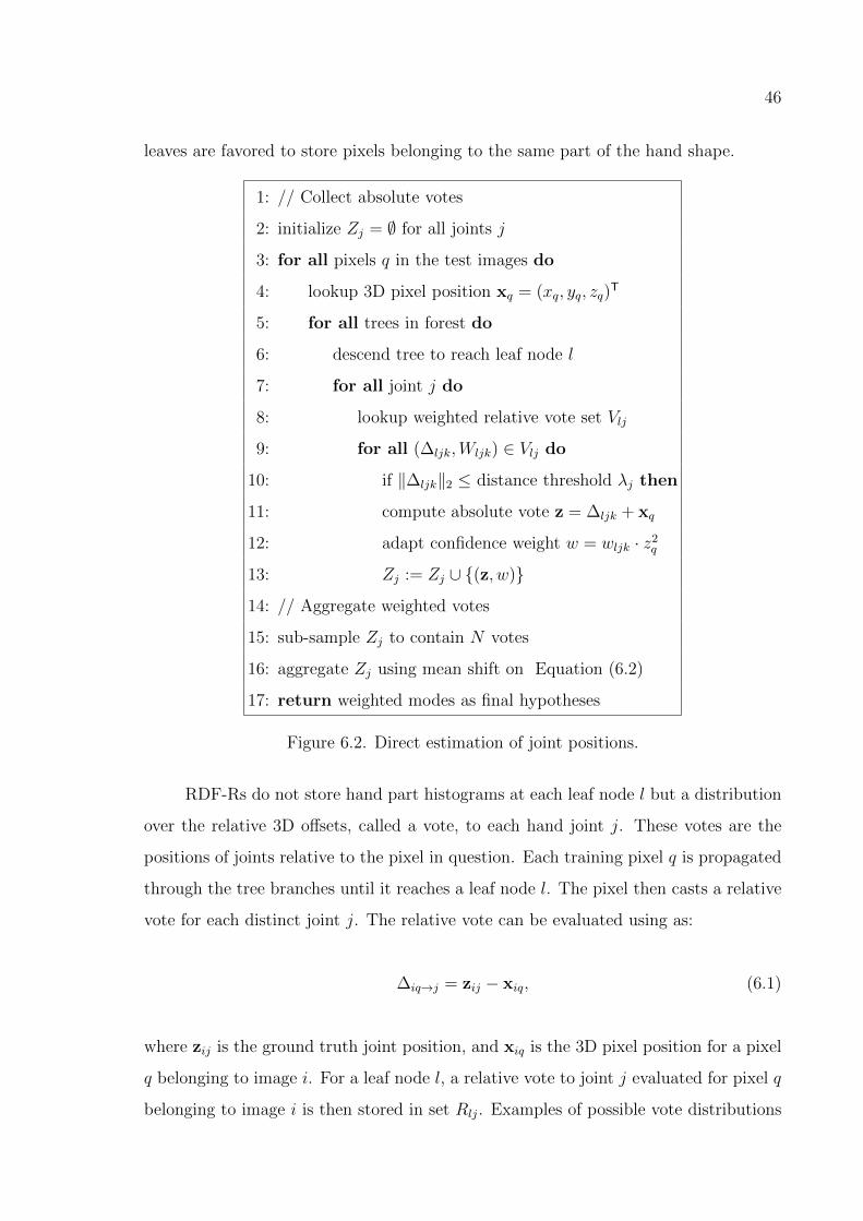
46
leaves are favored to store pixels belonging to the same part of the hand shape.
1: // Collect absolute votes
2: initialize Zj = ∅ for all joints j
3: for all pixels q in the test images do
4: lookup 3D pixel position xq = (xq, yq, zq)T
5: for all trees in forest do
6: descend tree to reach leaf node l
7: for all joint j do
8: lookup weighted relative vote set Vlj
9: for all (∆ljk,Wljk) ∈ Vlj do
10: if ‖∆ljk‖2 ≤ distance threshold λj then
11: compute absolute vote z = ∆ljk + xq
12: adapt confidence weight w = wljk · z2q13: Zj := Zj ∪ {(z, w)}
14: // Aggregate weighted votes
15: sub-sample Zj to contain N votes
16: aggregate Zj using mean shift on Equation (6.2)
17: return weighted modes as final hypotheses
Figure 6.2. Direct estimation of joint positions.
RDF-Rs do not store hand part histograms at each leaf node l but a distribution
over the relative 3D offsets, called a vote, to each hand joint j. These votes are the
positions of joints relative to the pixel in question. Each training pixel q is propagated
through the tree branches until it reaches a leaf node l. The pixel then casts a relative
vote for each distinct joint j. The relative vote can be evaluated using as:
∆iq→j = zij − xiq, (6.1)
where zij is the ground truth joint position, and xiq is the 3D pixel position for a pixel
q belonging to image i. For a leaf node l, a relative vote to joint j evaluated for pixel q
belonging to image i is then stored in set Rlj. Examples of possible vote distributions
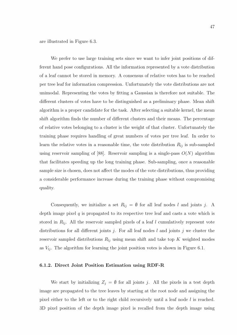
47
are illustrated in Figure 6.3.
We prefer to use large training sets since we want to infer joint positions of dif-
ferent hand pose configurations. All the information represented by a vote distribution
of a leaf cannot be stored in memory. A consensus of relative votes has to be reached
per tree leaf for information compression. Unfortunately the vote distributions are not
unimodal. Representing the votes by fitting a Gaussian is therefore not suitable. The
different clusters of votes have to be distinguished as a preliminary phase. Mean shift
algorithm is a proper candidate for the task. After selecting a suitable kernel, the mean
shift algorithm finds the number of different clusters and their means. The percentage
of relative votes belonging to a cluster is the weight of that cluster. Unfortunately the
training phase requires handling of great numbers of votes per tree leaf. In order to
learn the relative votes in a reasonable time, the vote distribution Rlj is sub-sampled
using reservoir sampling of [88]. Reservoir sampling is a single-pass O(N) algorithm
that facilitates speeding up the long training phase. Sub-sampling, once a reasonable
sample size is chosen, does not affect the modes of the vote distributions, thus providing
a considerable performance increase during the training phase without compromising
quality.
Consequently, we initialize a set Rlj = ∅ for all leaf nodes l and joints j. A
depth image pixel q is propagated to its respective tree leaf and casts a vote which is
stored in Rlj. All the reservoir sampled pixels of a leaf l cumulatively represent vote
distributions for all different joints j. For all leaf nodes l and joints j we cluster the
reservoir sampled distributions Rlj using mean shift and take top K weighted modes
as Vlj. The algorithm for learning the joint position votes is shown in Figure 6.1.
6.1.2. Direct Joint Position Estimation using RDF-R
We start by initializing Zj = ∅ for all joints j. All the pixels in a test depth
image are propagated to the tree leaves by starting at the root node and assigning the
pixel either to the left or to the right child recursively until a leaf node l is reached.
3D pixel position of the depth image pixel is recalled from the depth image using
48
Figure 6.3. Sample multi-modal vote distributions for three different joints. Vote
distributions may have multiple modes. Different colors indicate pixel clusters that
are assigned to the same mode found by mean shift.
xq = (xq, yq, zq)T. Each test-time depth pixel casts its per joint vote as represented by
the stored weighted relative vote set Vlj. Absolute vote coordinate is evaluated using
z = ∆ljk + xq. The vote is not cast if ‖∆ljk‖2 ≥ λj, where λj is a distance threshold
learned for each different hand joint. To aggregate the absolute votes Zj, for each joint
j we define a continuous distribution over world space using a Gaussian Parzen density
estimator such as
Pj(z′) =
∑(z,w)∈Zj
w. exp
(−∥∥∥∥z′ − zbj
∥∥∥∥22
), (6.2)
where bj is a learned per-joint bandwidth. Running mean shift using Equation 6.2
produces the weighted modes as final hypotheses. The layout of inference algorithm is
shown in Figure 6.2. A preliminary comparison of classification and regression based
methods on a single pose is illustrated in Figure 6.4.
6.2. Hierarchical Mode Selection using Geometry Constraints (RDF-R+)
RDF-R method outputs posterior distributions of possible joint locations. Even
though using the global modes of the multi-modal distributions seems to be the most
straightforward approach, the correct position of the joint often corresponds to a local
mode. However, considering local modes for the joint positions results in multiple
skeletal configuration candidates, instead of a single one given by the global modes. For
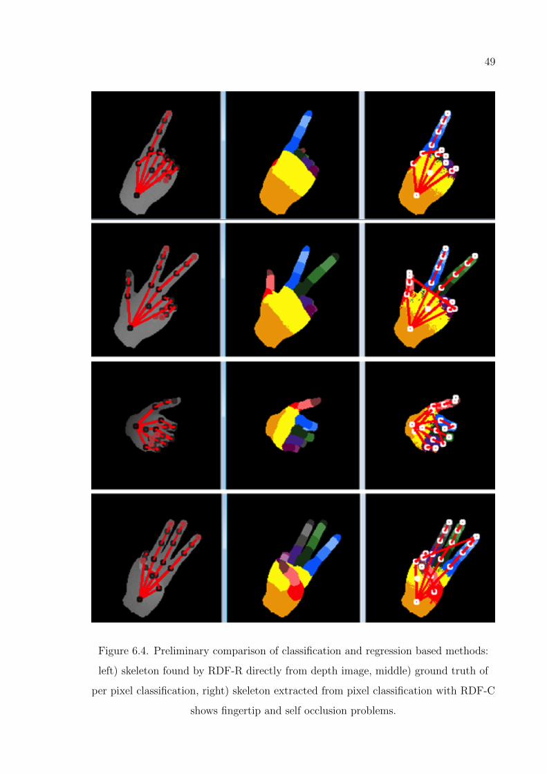
49
Figure 6.4. Preliminary comparison of classification and regression based methods:
left) skeleton found by RDF-R directly from depth image, middle) ground truth of
per pixel classification, right) skeleton extracted from pixel classification with RDF-C
shows fingertip and self occlusion problems.
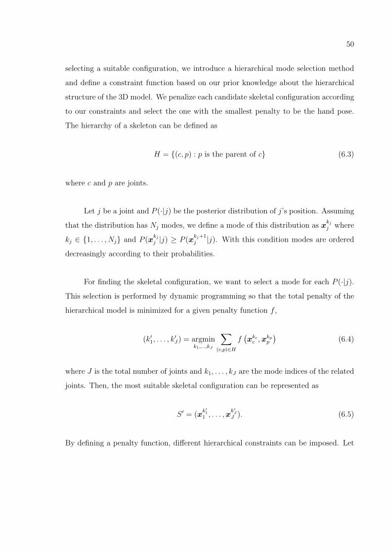
50
selecting a suitable configuration, we introduce a hierarchical mode selection method
and define a constraint function based on our prior knowledge about the hierarchical
structure of the 3D model. We penalize each candidate skeletal configuration according
to our constraints and select the one with the smallest penalty to be the hand pose.
The hierarchy of a skeleton can be defined as
H = {(c, p) : p is the parent of c} (6.3)
where c and p are joints.
Let j be a joint and P (·|j) be the posterior distribution of j’s position. Assuming
that the distribution has Nj modes, we define a mode of this distribution as xkjj where
kj ∈ {1, . . . , Nj} and P (xkjj |j) ≥ P (x
kj+1j |j). With this condition modes are ordered
decreasingly according to their probabilities.
For finding the skeletal configuration, we want to select a mode for each P (·|j).
This selection is performed by dynamic programming so that the total penalty of the
hierarchical model is minimized for a given penalty function f ,
(k′1, . . . , k′J) = argmin
k1,...,kJ
∑(c,p)∈H
f(xkcc ,x
kpp
)(6.4)
where J is the total number of joints and k1, . . . , kJ are the mode indices of the related
joints. Then, the most suitable skeletal configuration can be represented as
S ′ = (xk′11 , . . . ,x
k′JJ ). (6.5)
By defining a penalty function, different hierarchical constraints can be imposed. Let
51
us define two different penalty functions
f1(xicc ,x
ipp
)=
0, ic = 1 and ip = 1
1, otherwise
(6.6)
f2(xicc ,x
ipp
)=(||xic
c − xipp || − bcp
)2(6.7)
where bcp is the expected length of the bone between the joints c and p.
Since xkj s are ordered according to their probability, the global mode of the pos-
terior distribution is x1j . Thus, f1 behaves as the global mode finding approach used
by [24]. f2 tries to select the modes such that the distance between them is as close as
possible to the expected bone length.
An example of the improvement made by RDF-R+ method is shown in Figure 6.5
which shows the vote distribution for tip of the index finger. As clearly seen, there are
two different local modes in the distribution. The global mode is not the correct one to
be selected. RDF-R wrongly selects the global mode whereas RDF-R+ considers the
hierarchical dependencies of the joints and finds the appropriate local mode successfully.
In this section, we introduced a novel hierarchical mode selection method which
introduces the use of constraints imposed by the hand skeleton geometry. RDF-Rs ex-
tract multi-modal joint position distributions per joint. They only consider the global
mode. However, disregarded local modes of the joint distribution provide invaluable
information in the case of self-occlusions and missing data. Knowing all joint configura-
tions are sampled from the same skeletal constraints provides a strong prior knowledge
about the hierarchy of the modes over different joints. We investigate possible skele-
ton configurations that fit not only on the global modes but also on the local modes.
The probable configurations are then filtered out using distance constraints based on
a priori positions from the hand skeleton model. For the single frame estimation case,
the best skeletal configuration is selected to be the hand pose using dynamic program-
ming. In addition to that we also propose a low dimensional GPLVM based manifold
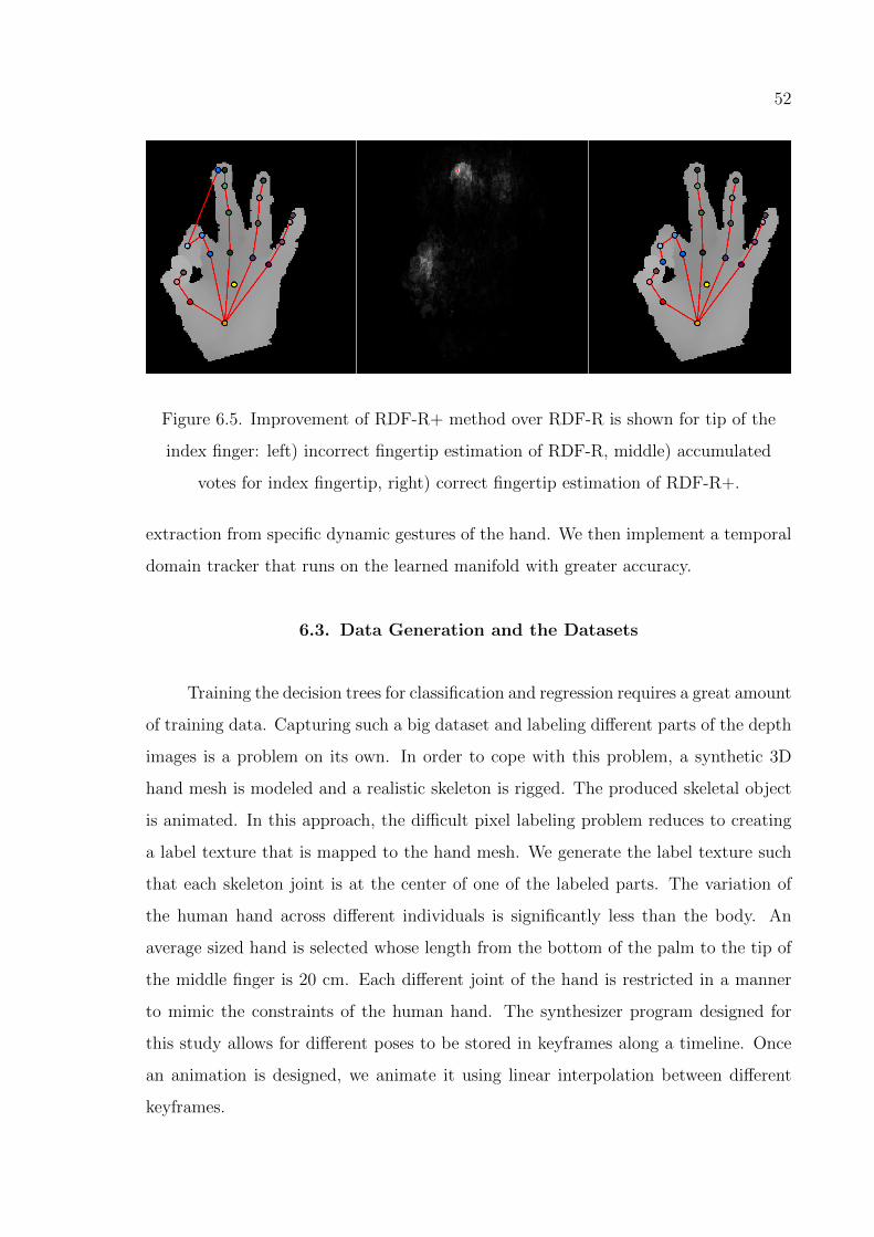
52
Figure 6.5. Improvement of RDF-R+ method over RDF-R is shown for tip of the
index finger: left) incorrect fingertip estimation of RDF-R, middle) accumulated
votes for index fingertip, right) correct fingertip estimation of RDF-R+.
extraction from specific dynamic gestures of the hand. We then implement a temporal
domain tracker that runs on the learned manifold with greater accuracy.
6.3. Data Generation and the Datasets
Training the decision trees for classification and regression requires a great amount
of training data. Capturing such a big dataset and labeling different parts of the depth
images is a problem on its own. In order to cope with this problem, a synthetic 3D
hand mesh is modeled and a realistic skeleton is rigged. The produced skeletal object
is animated. In this approach, the difficult pixel labeling problem reduces to creating
a label texture that is mapped to the hand mesh. We generate the label texture such
that each skeleton joint is at the center of one of the labeled parts. The variation of
the human hand across different individuals is significantly less than the body. An
average sized hand is selected whose length from the bottom of the palm to the tip of
the middle finger is 20 cm. Each different joint of the hand is restricted in a manner
to mimic the constraints of the human hand. The synthesizer program designed for
this study allows for different poses to be stored in keyframes along a timeline. Once
an animation is designed, we animate it using linear interpolation between different
keyframes.
53
In this chapter, we use 40 different hand poses. Poses are mainly selected from
the American Sign Language alphabet. 26 poses represent the letters from A to Z,
and 10 poses are for the numbers between 1 and 10. We also include four widely used
hand poses, namely the closed-hand, open-hand, approval gesture, and all finger tips
touching pose. For each pose, the model is rotated up to 32, 64, and 64 degrees along
the x, y, and z axes, respectively. Various samples are collected for different angles
with steps of six degrees. Center of the palm is always aligned with the center of the
images created. We also add Gaussian depth noise to the depth image pixels with a
mean of 10 mm, and a standard deviation of 5 for improving the generalization of the
trained classifiers. During hand pose configuration setup, Gaussian noise is introduced
to the angles of the skeleton for the unconstrained degree of freedoms with a mean of 2
degrees and a standard deviation of 1 degree. The resulting training (TRAIN) dataset
consists of 29766 image samples. Rendered depth and label images are 160x160 pixels
in resolution. In Figure 6.6, we show sample frames from the TRAIN dataset.
Training and validation are done on the TRAIN dataset using 10–fold cross val-
idation. For testing the performance of different methods, we created two different
datasets. The first one is the cropped (CROP) dataset. It is generated by retaining
the center 80x80 pixels and erasing the outer pixels of each image from the TRAIN
dataset. On the average, 81.09% of the pixels from each image are kept with a standard
deviation of 8.91. The CROP dataset is used for testing the performance of different
methods under missing data conditions.
The second test dataset is the Rock-Paper-Scissors-Lizard-Spock (RPSLS) dataset.
The Rock-Paper-Scissors-Lizard-Spock game is invented by [89]. The RPSLS dataset
is a completely new dataset synthesized from 5 different well-known poses not con-
tained in the training set. All possible transitions between pose pairs are considered
and animated using 3 frames per transition. The same rotation conditions are also
applied to the pose animations, resulting in a dataset of 30492 images with 160x160
resolution. The poses of the RPSLS dataset are not used during the training of the
decision trees. This dataset is used to benchmark the generalization performance of
different methods.
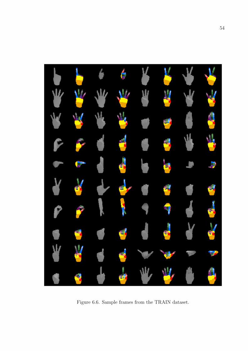
54
Figure 6.6. Sample frames from the TRAIN dataset.
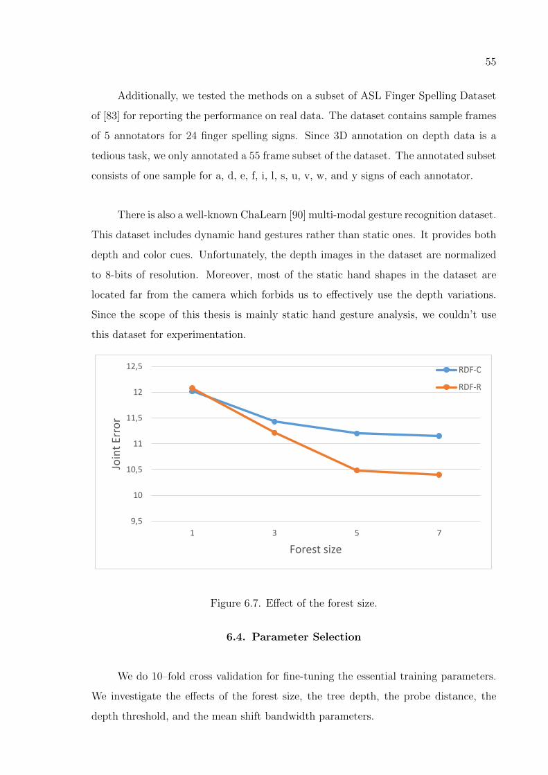
55
Additionally, we tested the methods on a subset of ASL Finger Spelling Dataset
of [83] for reporting the performance on real data. The dataset contains sample frames
of 5 annotators for 24 finger spelling signs. Since 3D annotation on depth data is a
tedious task, we only annotated a 55 frame subset of the dataset. The annotated subset
consists of one sample for a, d, e, f, i, l, s, u, v, w, and y signs of each annotator.
There is also a well-known ChaLearn [90] multi-modal gesture recognition dataset.
This dataset includes dynamic hand gestures rather than static ones. It provides both
depth and color cues. Unfortunately, the depth images in the dataset are normalized
to 8-bits of resolution. Moreover, most of the static hand shapes in the dataset are
located far from the camera which forbids us to effectively use the depth variations.
Since the scope of this thesis is mainly static hand gesture analysis, we couldn’t use
this dataset for experimentation.
9,5
10
10,5
11
11,5
12
12,5
1 3 5 7
Join
t Er
ror
Forest size
RDF-C
RDF-R
Figure 6.7. Effect of the forest size.
6.4. Parameter Selection
We do 10–fold cross validation for fine-tuning the essential training parameters.
We investigate the effects of the forest size, the tree depth, the probe distance, the
depth threshold, and the mean shift bandwidth parameters.
56
0
5
10
15
20
25
7 9 11 13 15 17 19 21 23 25
Join
t Er
ror
Tree depth
RDF-C
RDF-R
Figure 6.8. Effect of the tree depth.
6.4.1. The Effect of the Forest Size
An advantage of random forests is that the inference performance can be en-
hanced by combining multiple random trees. Both the generalization capability and
the accuracy of the inference improves as the number of trees used is increased. There
is a trade-off between inference time and the inference accuracy. Figure 6.7 shows the
effect of number of trees on the accuracy of the system. Accuracy, recognition time,
and memory usage are jointly optimized when the number of trees is selected to be 5.
6.4.2. The Effect of the Tree Depth
The depth of the trees is also an essential parameter. The representation capa-
bility increases as the depth of the trees increase. Unfortunately, increasing the depth
of the trees also increases the inference time. Selecting an optimal depth is important
for balancing the inference accuracy and the recognition time. In addition to that, the
memory requirement also increases exponentially. If the training data complexity and
size are not adequate for the utilization of the desired tree depth, numerous empty
sub-branches in the forest structure appear. This under-utilization causes ineffective
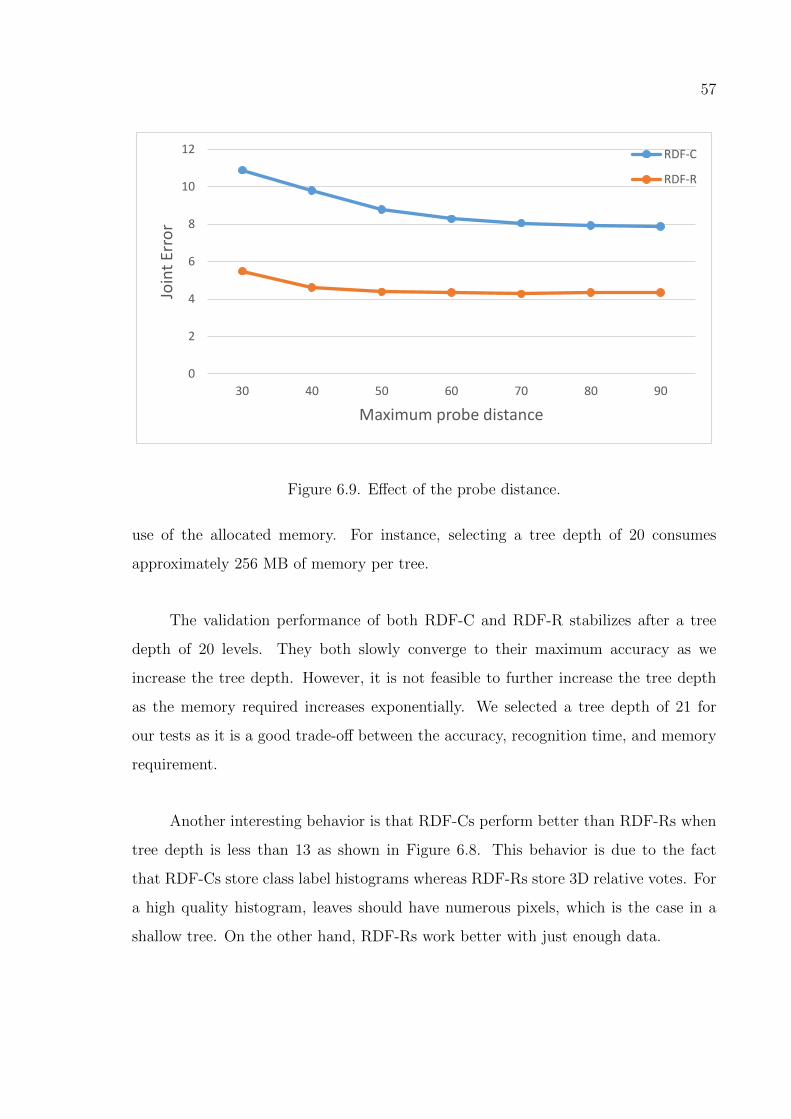
57
0
2
4
6
8
10
12
30 40 50 60 70 80 90
Join
t Er
ror
Maximum probe distance
RDF-C
RDF-R
Figure 6.9. Effect of the probe distance.
use of the allocated memory. For instance, selecting a tree depth of 20 consumes
approximately 256 MB of memory per tree.
The validation performance of both RDF-C and RDF-R stabilizes after a tree
depth of 20 levels. They both slowly converge to their maximum accuracy as we
increase the tree depth. However, it is not feasible to further increase the tree depth
as the memory required increases exponentially. We selected a tree depth of 21 for
our tests as it is a good trade-off between the accuracy, recognition time, and memory
requirement.
Another interesting behavior is that RDF-Cs perform better than RDF-Rs when
tree depth is less than 13 as shown in Figure 6.8. This behavior is due to the fact
that RDF-Cs store class label histograms whereas RDF-Rs store 3D relative votes. For
a high quality histogram, leaves should have numerous pixels, which is the case in a
shallow tree. On the other hand, RDF-Rs work better with just enough data.
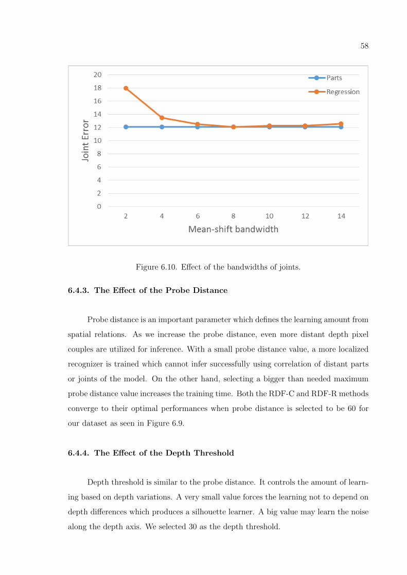
58
Figure 6.10. Effect of the bandwidths of joints.
6.4.3. The Effect of the Probe Distance
Probe distance is an important parameter which defines the learning amount from
spatial relations. As we increase the probe distance, even more distant depth pixel
couples are utilized for inference. With a small probe distance value, a more localized
recognizer is trained which cannot infer successfully using correlation of distant parts
or joints of the model. On the other hand, selecting a bigger than needed maximum
probe distance value increases the training time. Both the RDF-C and RDF-R methods
converge to their optimal performances when probe distance is selected to be 60 for
our dataset as seen in Figure 6.9.
6.4.4. The Effect of the Depth Threshold
Depth threshold is similar to the probe distance. It controls the amount of learn-
ing based on depth variations. A very small value forces the learning not to depend on
depth differences which produces a silhouette learner. A big value may learn the noise
along the depth axis. We selected 30 as the depth threshold.
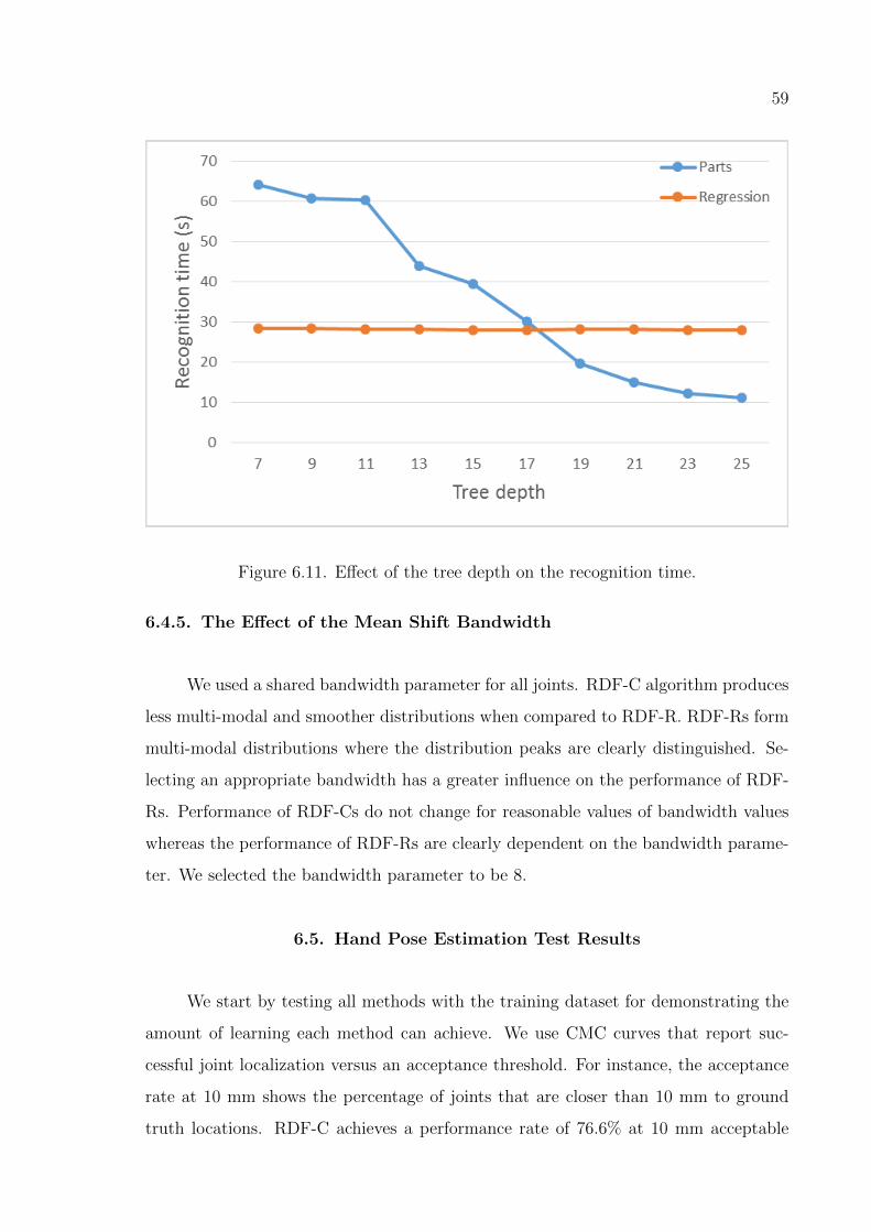
59
Figure 6.11. Effect of the tree depth on the recognition time.
6.4.5. The Effect of the Mean Shift Bandwidth
We used a shared bandwidth parameter for all joints. RDF-C algorithm produces
less multi-modal and smoother distributions when compared to RDF-R. RDF-Rs form
multi-modal distributions where the distribution peaks are clearly distinguished. Se-
lecting an appropriate bandwidth has a greater influence on the performance of RDF-
Rs. Performance of RDF-Cs do not change for reasonable values of bandwidth values
whereas the performance of RDF-Rs are clearly dependent on the bandwidth parame-
ter. We selected the bandwidth parameter to be 8.
6.5. Hand Pose Estimation Test Results
We start by testing all methods with the training dataset for demonstrating the
amount of learning each method can achieve. We use CMC curves that report suc-
cessful joint localization versus an acceptance threshold. For instance, the acceptance
rate at 10 mm shows the percentage of joints that are closer than 10 mm to ground
truth locations. RDF-C achieves a performance rate of 76.6% at 10 mm acceptable
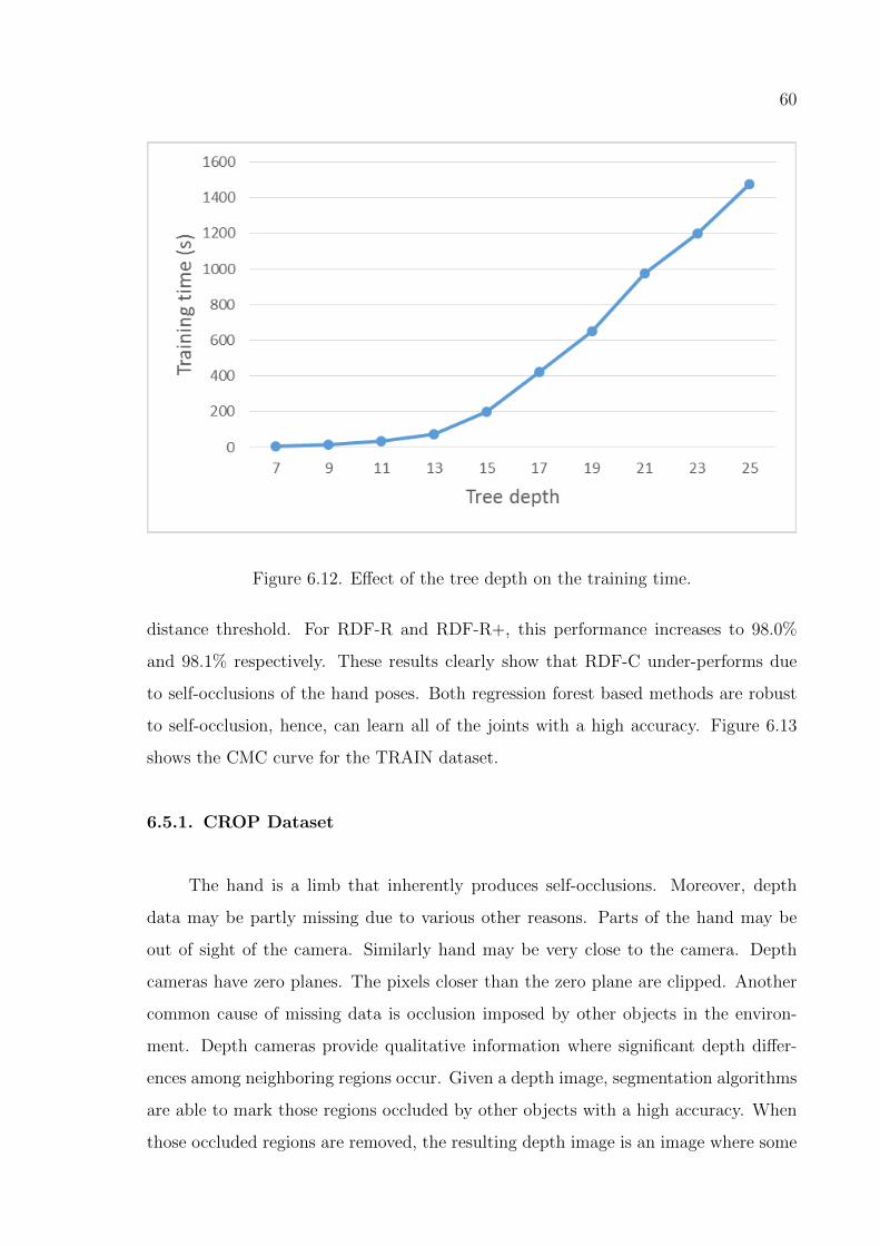
60
Figure 6.12. Effect of the tree depth on the training time.
distance threshold. For RDF-R and RDF-R+, this performance increases to 98.0%
and 98.1% respectively. These results clearly show that RDF-C under-performs due
to self-occlusions of the hand poses. Both regression forest based methods are robust
to self-occlusion, hence, can learn all of the joints with a high accuracy. Figure 6.13
shows the CMC curve for the TRAIN dataset.
6.5.1. CROP Dataset
The hand is a limb that inherently produces self-occlusions. Moreover, depth
data may be partly missing due to various other reasons. Parts of the hand may be
out of sight of the camera. Similarly hand may be very close to the camera. Depth
cameras have zero planes. The pixels closer than the zero plane are clipped. Another
common cause of missing data is occlusion imposed by other objects in the environ-
ment. Depth cameras provide qualitative information where significant depth differ-
ences among neighboring regions occur. Given a depth image, segmentation algorithms
are able to mark those regions occluded by other objects with a high accuracy. When
those occluded regions are removed, the resulting depth image is an image where some
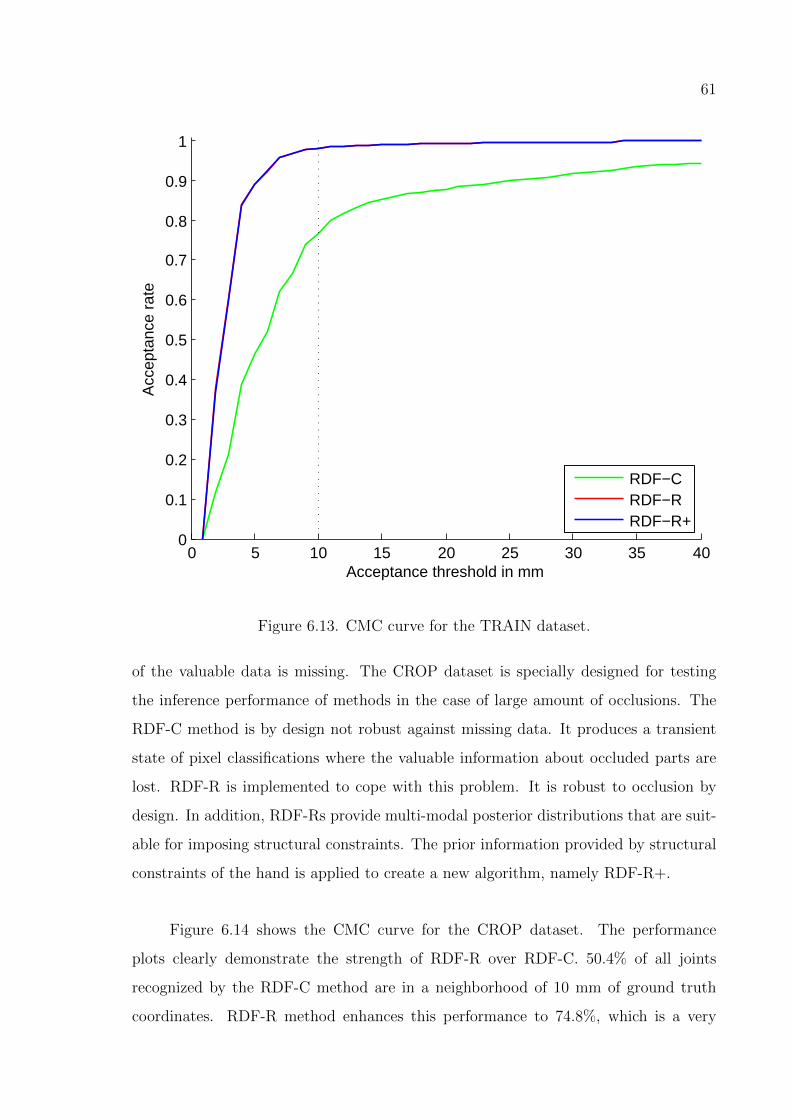
61
0 5 10 15 20 25 30 35 400
0.1
0.2
0.3
0.4
0.5
0.6
0.7
0.8
0.9
1
Acceptance threshold in mm
Acc
epta
nce
rate
RDF−CRDF−RRDF−R+
Figure 6.13. CMC curve for the TRAIN dataset.
of the valuable data is missing. The CROP dataset is specially designed for testing
the inference performance of methods in the case of large amount of occlusions. The
RDF-C method is by design not robust against missing data. It produces a transient
state of pixel classifications where the valuable information about occluded parts are
lost. RDF-R is implemented to cope with this problem. It is robust to occlusion by
design. In addition, RDF-Rs provide multi-modal posterior distributions that are suit-
able for imposing structural constraints. The prior information provided by structural
constraints of the hand is applied to create a new algorithm, namely RDF-R+.
Figure 6.14 shows the CMC curve for the CROP dataset. The performance
plots clearly demonstrate the strength of RDF-R over RDF-C. 50.4% of all joints
recognized by the RDF-C method are in a neighborhood of 10 mm of ground truth
coordinates. RDF-R method enhances this performance to 74.8%, which is a very
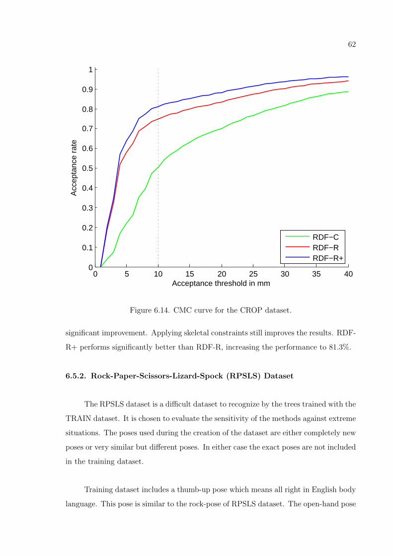
62
0 5 10 15 20 25 30 35 400
0.1
0.2
0.3
0.4
0.5
0.6
0.7
0.8
0.9
1
Acceptance threshold in mm
Acc
epta
nce
rate
RDF−CRDF−RRDF−R+
Figure 6.14. CMC curve for the CROP dataset.
significant improvement. Applying skeletal constraints still improves the results. RDF-
R+ performs significantly better than RDF-R, increasing the performance to 81.3%.
6.5.2. Rock-Paper-Scissors-Lizard-Spock (RPSLS) Dataset
The RPSLS dataset is a difficult dataset to recognize by the trees trained with the
TRAIN dataset. It is chosen to evaluate the sensitivity of the methods against extreme
situations. The poses used during the creation of the dataset are either completely new
poses or very similar but different poses. In either case the exact poses are not included
in the training dataset.
Training dataset includes a thumb-up pose which means all right in English body
language. This pose is similar to the rock-pose of RPSLS dataset. The open-hand pose
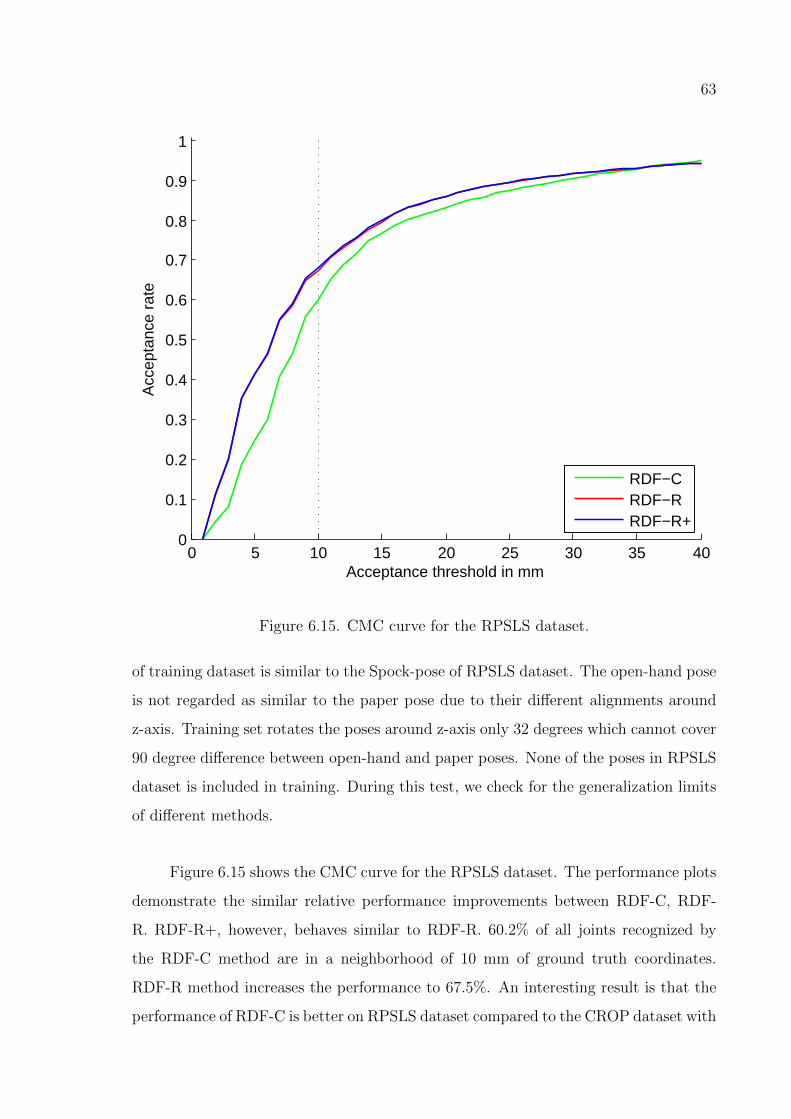
63
0 5 10 15 20 25 30 35 400
0.1
0.2
0.3
0.4
0.5
0.6
0.7
0.8
0.9
1
Acceptance threshold in mm
Acc
epta
nce
rate
RDF−CRDF−RRDF−R+
Figure 6.15. CMC curve for the RPSLS dataset.
of training dataset is similar to the Spock-pose of RPSLS dataset. The open-hand pose
is not regarded as similar to the paper pose due to their different alignments around
z-axis. Training set rotates the poses around z-axis only 32 degrees which cannot cover
90 degree difference between open-hand and paper poses. None of the poses in RPSLS
dataset is included in training. During this test, we check for the generalization limits
of different methods.
Figure 6.15 shows the CMC curve for the RPSLS dataset. The performance plots
demonstrate the similar relative performance improvements between RDF-C, RDF-
R. RDF-R+, however, behaves similar to RDF-R. 60.2% of all joints recognized by
the RDF-C method are in a neighborhood of 10 mm of ground truth coordinates.
RDF-R method increases the performance to 67.5%. An interesting result is that the
performance of RDF-C is better on RPSLS dataset compared to the CROP dataset with
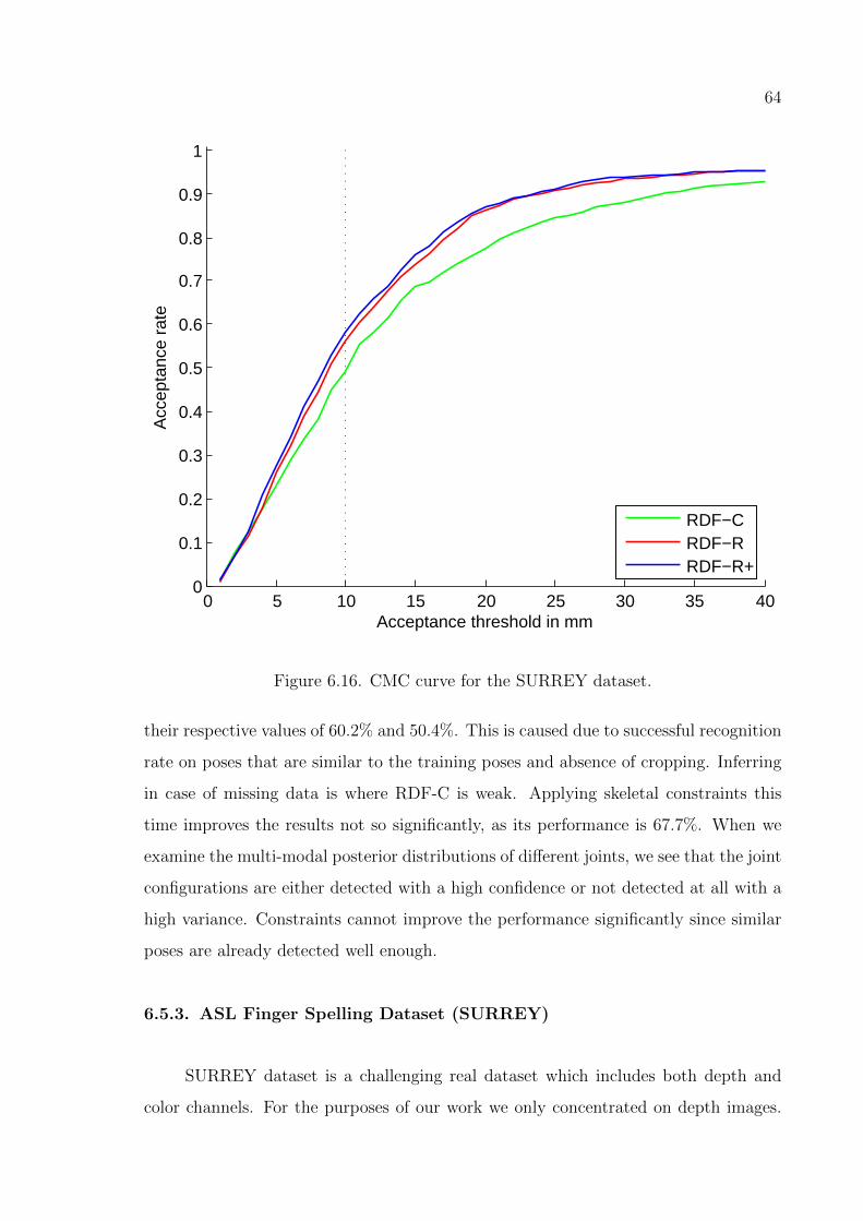
64
0 5 10 15 20 25 30 35 400
0.1
0.2
0.3
0.4
0.5
0.6
0.7
0.8
0.9
1
Acceptance threshold in mm
Acc
epta
nce
rate
RDF−CRDF−RRDF−R+
Figure 6.16. CMC curve for the SURREY dataset.
their respective values of 60.2% and 50.4%. This is caused due to successful recognition
rate on poses that are similar to the training poses and absence of cropping. Inferring
in case of missing data is where RDF-C is weak. Applying skeletal constraints this
time improves the results not so significantly, as its performance is 67.7%. When we
examine the multi-modal posterior distributions of different joints, we see that the joint
configurations are either detected with a high confidence or not detected at all with a
high variance. Constraints cannot improve the performance significantly since similar
poses are already detected well enough.
6.5.3. ASL Finger Spelling Dataset (SURREY)
SURREY dataset is a challenging real dataset which includes both depth and
color channels. For the purposes of our work we only concentrated on depth images.
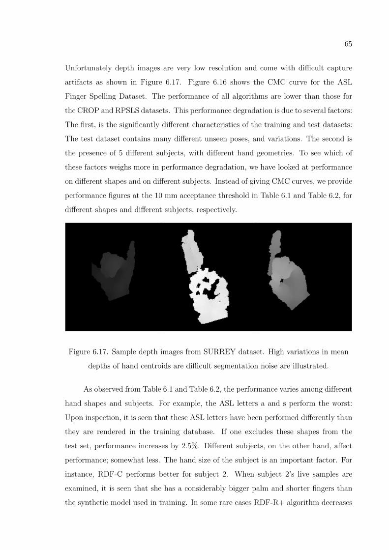
65
Unfortunately depth images are very low resolution and come with difficult capture
artifacts as shown in Figure 6.17. Figure 6.16 shows the CMC curve for the ASL
Finger Spelling Dataset. The performance of all algorithms are lower than those for
the CROP and RPSLS datasets. This performance degradation is due to several factors:
The first, is the significantly different characteristics of the training and test datasets:
The test dataset contains many different unseen poses, and variations. The second is
the presence of 5 different subjects, with different hand geometries. To see which of
these factors weighs more in performance degradation, we have looked at performance
on different shapes and on different subjects. Instead of giving CMC curves, we provide
performance figures at the 10 mm acceptance threshold in Table 6.1 and Table 6.2, for
different shapes and different subjects, respectively.
Figure 6.17. Sample depth images from SURREY dataset. High variations in mean
depths of hand centroids are difficult segmentation noise are illustrated.
As observed from Table 6.1 and Table 6.2, the performance varies among different
hand shapes and subjects. For example, the ASL letters a and s perform the worst:
Upon inspection, it is seen that these ASL letters have been performed differently than
they are rendered in the training database. If one excludes these shapes from the
test set, performance increases by 2.5%. Different subjects, on the other hand, affect
performance; somewhat less. The hand size of the subject is an important factor. For
instance, RDF-C performs better for subject 2. When subject 2’s live samples are
examined, it is seen that she has a considerably bigger palm and shorter fingers than
the synthetic model used in training. In some rare cases RDF-R+ algorithm decreases
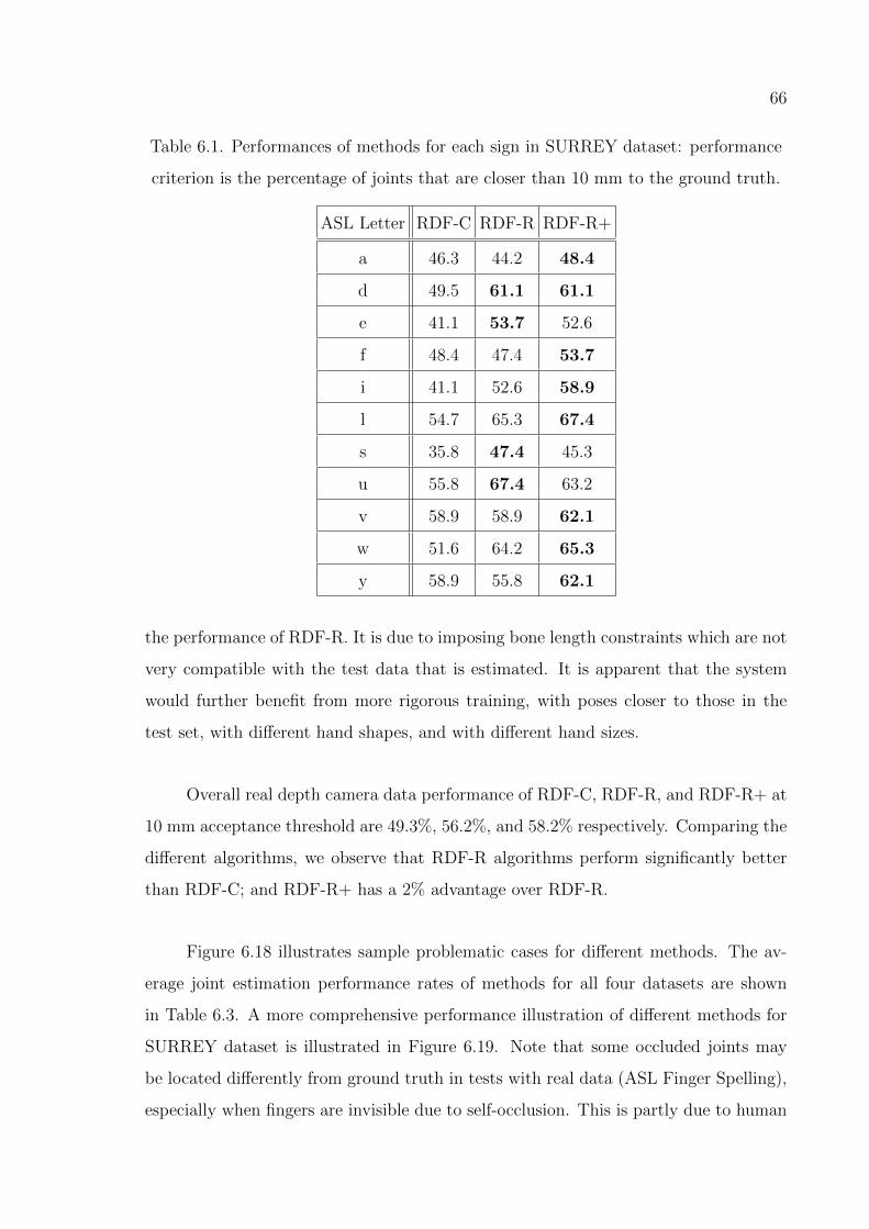
66
Table 6.1. Performances of methods for each sign in SURREY dataset: performance
criterion is the percentage of joints that are closer than 10 mm to the ground truth.
ASL Letter RDF-C RDF-R RDF-R+
a 46.3 44.2 48.4
d 49.5 61.1 61.1
e 41.1 53.7 52.6
f 48.4 47.4 53.7
i 41.1 52.6 58.9
l 54.7 65.3 67.4
s 35.8 47.4 45.3
u 55.8 67.4 63.2
v 58.9 58.9 62.1
w 51.6 64.2 65.3
y 58.9 55.8 62.1
the performance of RDF-R. It is due to imposing bone length constraints which are not
very compatible with the test data that is estimated. It is apparent that the system
would further benefit from more rigorous training, with poses closer to those in the
test set, with different hand shapes, and with different hand sizes.
Overall real depth camera data performance of RDF-C, RDF-R, and RDF-R+ at
10 mm acceptance threshold are 49.3%, 56.2%, and 58.2% respectively. Comparing the
different algorithms, we observe that RDF-R algorithms perform significantly better
than RDF-C; and RDF-R+ has a 2% advantage over RDF-R.
Figure 6.18 illustrates sample problematic cases for different methods. The av-
erage joint estimation performance rates of methods for all four datasets are shown
in Table 6.3. A more comprehensive performance illustration of different methods for
SURREY dataset is illustrated in Figure 6.19. Note that some occluded joints may
be located differently from ground truth in tests with real data (ASL Finger Spelling),
especially when fingers are invisible due to self-occlusion. This is partly due to human
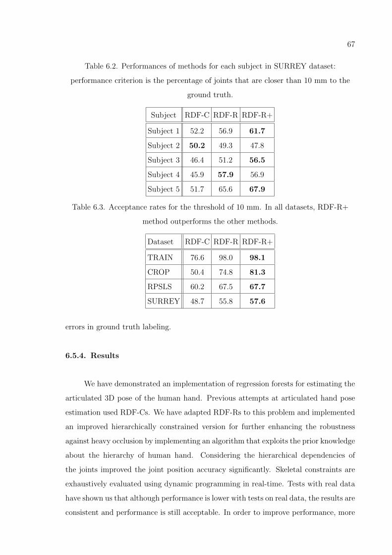
67
Table 6.2. Performances of methods for each subject in SURREY dataset:
performance criterion is the percentage of joints that are closer than 10 mm to the
ground truth.
Subject RDF-C RDF-R RDF-R+
Subject 1 52.2 56.9 61.7
Subject 2 50.2 49.3 47.8
Subject 3 46.4 51.2 56.5
Subject 4 45.9 57.9 56.9
Subject 5 51.7 65.6 67.9
Table 6.3. Acceptance rates for the threshold of 10 mm. In all datasets, RDF-R+
method outperforms the other methods.
Dataset RDF-C RDF-R RDF-R+
TRAIN 76.6 98.0 98.1
CROP 50.4 74.8 81.3
RPSLS 60.2 67.5 67.7
SURREY 48.7 55.8 57.6
errors in ground truth labeling.
6.5.4. Results
We have demonstrated an implementation of regression forests for estimating the
articulated 3D pose of the human hand. Previous attempts at articulated hand pose
estimation used RDF-Cs. We have adapted RDF-Rs to this problem and implemented
an improved hierarchically constrained version for further enhancing the robustness
against heavy occlusion by implementing an algorithm that exploits the prior knowledge
about the hierarchy of human hand. Considering the hierarchical dependencies of
the joints improved the joint position accuracy significantly. Skeletal constraints are
exhaustively evaluated using dynamic programming in real-time. Tests with real data
have shown us that although performance is lower with tests on real data, the results are
consistent and performance is still acceptable. In order to improve performance, more
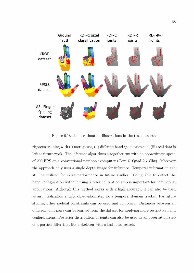
68
Figure 6.18. Joint estimation illustrations in the test datasets.
rigorous training with (i) more poses, (ii) different hand geometries and, (iii) real data is
left as future work. The inference algorithms altogether run with an approximate speed
of 200 FPS on a conventional notebook computer (Core i7 Quad 2.7 Ghz). Moreover
the approach only uses a single depth image for inference. Temporal information can
still be utilized for extra performance in future studies. Being able to detect the
hand configuration without using a prior calibration step is important for commercial
applications. Although this method works with a high accuracy, it can also be used
as an initialization and/or observation step for a temporal domain tracker. For future
studies, other skeletal constraints can be used and combined. Distances between all
different joint pairs can be learned from the dataset for applying more restrictive hand
configurations. Posterior distribution of joints can also be used as an observation step
of a particle filter that fits a skeleton with a fast local search.
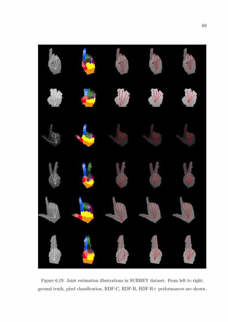
69
Figure 6.19. Joint estimation illustrations in SURREY dataset. From left to right;
ground truth, pixel classification, RDF-C, RDF-R, RDF-R+ performances are shown.
70
7. TRACKING DYNAMIC HAND GESTURES
The methods discussed in previous chapters capture the pose configuration of
the hand joints without using any temporal information. While this ability is essential
for re-initialization of the pose estimation framework, it would be better if one could
incorporate the temporal information using tracking. However, the hand pose vector
is high dimensional and tracking in this space causes errors. While the hand can take
arbitrary poses, it is well known that the correlation between joint angles is very high.
Therefore, it is a good idea to reduce the dimensionality and to track hand pose on a
reduced dimensionality manifold. Moreover, extracting a manifold provides additional
benefits that it also captures the inter-dependencies of hand joint hierarchy. Previous
methods such as RDF-C, RDF-H, RDF-R, all consider the joints as independent. RDF-
R+ tries to force hand hierarchy into the pose configuration search but it is still possible
to extract an unrelated pose.
In this section, GPLVM dimensionality reduction method is considered for reduc-
ing the dimensionality of the pose configuration model of a specific hand motion to a
2D manifold. Most pose estimation applications can benefit from the additional track-
ing performance gained by the prior knowledge of the underlying hand gesture. We
use the GPLVM to represent the prior knowledge in terms of a hand gesture manifold.
We first start by summarizing GPLVM in Section 7.2 as published in [72]. In Sec-
tion 7.3, we discuss a suitable representation of pose configuration. Learning the mani-
fold of hand gesture is mentioned in Section 7.4. Projecting a pose configuration space
vector onto the extracted manifold is explained in Section 7.5. We conclude by applying
Kalman Filter in Section 7.6 and presenting our experiment results in Section 7.7.
7.1. Gaussian Processes
Gaussian Processes (GP) [91] are generalizations of Gaussian distributions defined
over infinite index sets. Thereby a GP can be used to specify distribution over functions.
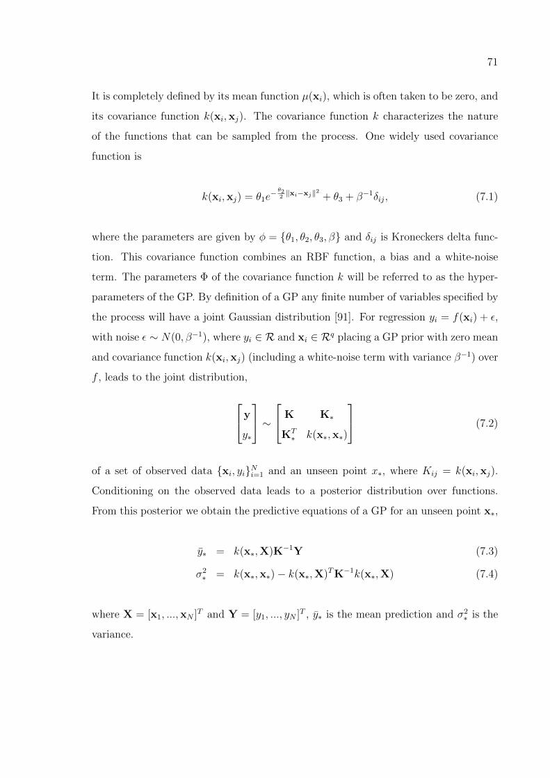
71
It is completely defined by its mean function µ(xi), which is often taken to be zero, and
its covariance function k(xi,xj). The covariance function k characterizes the nature
of the functions that can be sampled from the process. One widely used covariance
function is
k(xi,xj) = θ1e− θ2
2‖xi−xj‖2 + θ3 + β−1δij, (7.1)
where the parameters are given by φ = {θ1, θ2, θ3, β} and δij is Kroneckers delta func-
tion. This covariance function combines an RBF function, a bias and a white-noise
term. The parameters Φ of the covariance function k will be referred to as the hyper-
parameters of the GP. By definition of a GP any finite number of variables specified by
the process will have a joint Gaussian distribution [91]. For regression yi = f(xi) + ε,
with noise ε ∼ N(0, β−1), where yi ∈ R and xi ∈ Rq placing a GP prior with zero mean
and covariance function k(xi,xj) (including a white-noise term with variance β−1) over
f , leads to the joint distribution,
y
y∗
∼ K K∗
KT∗ k(x∗,x∗)
(7.2)
of a set of observed data {xi, yi}Ni=1 and an unseen point x∗, where Kij = k(xi,xj).
Conditioning on the observed data leads to a posterior distribution over functions.
From this posterior we obtain the predictive equations of a GP for an unseen point x∗,
y∗ = k(x∗,X)K−1Y (7.3)
σ2∗ = k(x∗,x∗)− k(x∗,X)TK−1k(x∗,X) (7.4)
where X = [x1, ...,xN ]T and Y = [y1, ..., yN ]T , y∗ is the mean prediction and σ2∗ is the
variance.
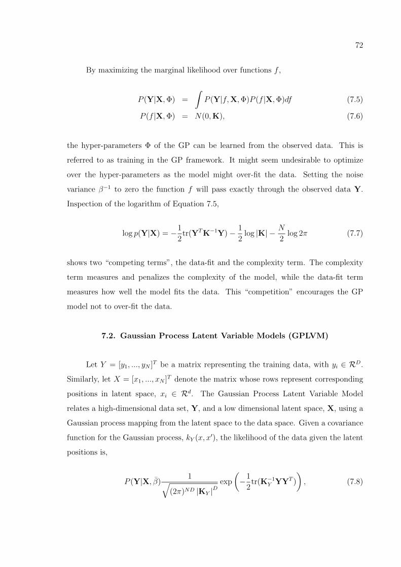
72
By maximizing the marginal likelihood over functions f ,
P (Y|X,Φ) =
∫P (Y|f,X,Φ)P (f |X,Φ)df (7.5)
P (f |X,Φ) = N(0,K), (7.6)
the hyper-parameters Φ of the GP can be learned from the observed data. This is
referred to as training in the GP framework. It might seem undesirable to optimize
over the hyper-parameters as the model might over-fit the data. Setting the noise
variance β−1 to zero the function f will pass exactly through the observed data Y.
Inspection of the logarithm of Equation 7.5,
log p(Y|X) = −1
2tr(YTK−1Y)− 1
2log |K| − N
2log 2π (7.7)
shows two “competing terms”, the data-fit and the complexity term. The complexity
term measures and penalizes the complexity of the model, while the data-fit term
measures how well the model fits the data. This “competition” encourages the GP
model not to over-fit the data.
7.2. Gaussian Process Latent Variable Models (GPLVM)
Let Y = [y1, ..., yN ]T be a matrix representing the training data, with yi ∈ RD.
Similarly, let X = [x1, ..., xN ]T denote the matrix whose rows represent corresponding
positions in latent space, xi ∈ Rd. The Gaussian Process Latent Variable Model
relates a high-dimensional data set, Y, and a low dimensional latent space, X, using a
Gaussian process mapping from the latent space to the data space. Given a covariance
function for the Gaussian process, kY (x, x′), the likelihood of the data given the latent
positions is,
P (Y|X, β)1√
(2π)ND |KY |Dexp
(−1
2tr(K−1Y YYT )
), (7.8)
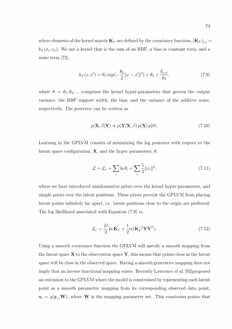
73
where elements of the kernel matrix KY are defined by the covariance function, (KY )i,j =
kY (xi, xj). We use a kernel that is the sum of an RBF, a bias or constant term, and a
noise term [72].
kY (x, x′) = θ1 exp(−θ22‖x− x′‖2) + θ3 +
δx,x′
θ4, (7.9)
where θ = θ1, θ2, ... comprises the kernel hyper-parameters that govern the output
variance, the RBF support width, the bias, and the variance of the additive noise,
respectively. The posterior can be written as
p(X, β|Y) ∝ p(Y|X, β) p(X) p(θ). (7.10)
Learning in the GPLVM consists of minimizing the log posterior with respect to the
latent space configuration, X, and the hyper parameters, θ,
L = Lr +∑i
ln θi +∑i
1
2‖xi‖2, (7.11)
where we have introduced uninformative priors over the kernel hyper-parameters, and
simple priors over the latent positions. These priors prevent the GPLVM from placing
latent points infinitely far apart, i.e. latent positions close to the origin are preferred.
The log likelihood associated with Equation (7.9) is,
Lr =D
2ln KY +
1
2tr(K−1Y YYT ). (7.12)
Using a smooth covariance function the GPLVM will specify a smooth mapping from
the latent space X to the observation space Y, this means that points close in the latent
space will be close in the observed space. Having a smooth generative mapping does not
imply that an inverse functional mapping exists. Recently Lawrence et al. [92]proposed
an extension to the GPLVM where the model is constrained by representing each latent
point as a smooth parametric mapping from its corresponding observed data point,
xi = g(yi,W), where W is the mapping parameter set. This constrains points that
74
are close in the observed space to also be close in the latent space. The mapping from
observed data Y to X is called the back-constraint.
7.3. Pose Representation Favorable for Dimensionality Reduction
GPLVM is selected as the non-linear manifold extraction tool since its behavior
is well studied in recent studies. Its pose interpolation capability is especially high as
presented in [93]. Our framework depends on good interpolation performance since it
is infeasible to train with all the possible hand pose configurations. The framework
designed must be able to generalize for poses which are not in the training dataset of
manifold extraction, and GPLVM is a good candidate for having smooth interpolation
performance.
Pose configuration can be defined using various different methodologies. One
could store a 3D position of the root joint of the hand in the world coordinate space
and then proceed by storing the relative angles of each degree of freedom per hand joint.
Despite its compressed representation, this kind of pose definition is hard to utilize since
even small errors in joints which are high in the hierarchy, accumulate. A very small
error in the root joint would affect the whole hand configuration considerably. On the
other hand, one can represent the hand pose configuration by storing all of the 3D
joint coordinates, in addition to the fingertip coordinates. This kind of representation
inherently includes the world space coordinates of the root hand joint, assuming that
the hand size is known. Moreover, this representation style is also compatible with
the RDF-C and RDF-R methods used for extracting the joint coordinates from a
single depth image. Therefore, we used 3D hand joint coordinates in combination with
fingertip coordinates as the pose configuration model.
Let us define xt ∈ Rm that represents the pose configuration of the human hand
skeleton, where m is a sufficiently large number that includes 3D coordinates of all
hand joints and all fingertips. In this work, m is set to be 60, which is enough to store
the 3D coordinates of 15 hand joints and 5 fingertips in order to define a valid hand
pose. Running a tracker on a high dimensional space such as Rm is a challenging task.
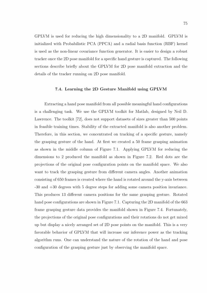
75
GPLVM is used for reducing the high dimensionality to a 2D manifold. GPLVM is
initialized with Probabilistic PCA (PPCA) and a radial basis function (RBF) kernel
is used as the non-linear covariance function generator. It is easier to design a robust
tracker once the 2D pose manifold for a specific hand gesture is captured. The following
sections describe briefly about the GPLVM for 2D pose manifold extraction and the
details of the tracker running on 2D pose manifold.
7.4. Learning the 2D Gesture Manifold using GPLVM
Extracting a hand pose manifold from all possible meaningful hand configurations
is a challenging task. We use the GPLVM toolkit for Matlab, designed by Neil D.
Lawrence. The toolkit [72], does not support datasets of sizes greater than 500 points
in feasible training times. Stability of the extracted manifold is also another problem.
Therefore, in this section, we concentrated on tracking of a specific gesture, namely
the grasping gesture of the hand. At first we created a 50 frame grasping animation
as shown in the middle column of Figure 7.1. Applying GPLVM for reducing the
dimensions to 2 produced the manifold as shown in Figure 7.2. Red dots are the
projections of the original pose configuration points on the manifold space. We also
want to track the grasping gesture from different camera angles. Another animation
consisting of 650 frames is created where the hand is rotated around the y-axis between
-30 and +30 degrees with 5 degree steps for adding some camera position invariance.
This produces 13 different camera positions for the same grasping gesture. Rotated
hand pose configurations are shown in Figure 7.1. Capturing the 2D manifold of the 663
frame grasping gesture data provides the manifold shown in Figure 7.4. Fortunately,
the projections of the original pose configurations and their rotations do not get mixed
up but display a nicely arranged set of 2D pose points on the manifold. This is a very
favorable behavior of GPLVM that will increase our inference power as the tracking
algorithm runs. One can understand the nature of the rotation of the hand and pose
configuration of the grasping gesture just by observing the manifold space.
76
7.5. Projecting the Pose Observations onto the Gesture Manifold
GPLVM has many advantages, however, it only provides one-way mapping from
the manifold space to the original space. Finding a mapping from the original space to
the manifold remains as a global search problem. Given a pose configuration, we used
a nearest neighbor classifier on the trained pose configurations for finding a suitable
projection on the manifold. L2 norm is used as the distance metric. Once the nearest
pose is found, its corresponding projection on the manifold is used as the starting
point of a local search. A small grid is located over the manifold space by taking the
starting point as its center. Size of the grid is adjusted so that it at least contains 8
different training points. The grid is searched with a brute force algorithm, at each
step mapping the 2D manifold point to its original space and evaluating the distance
from the ground truth using L2 norm. 2D coordinate which provides the smallest error
is selected as the 2D mapping of the original pose configuration. Local search grid is
illustrated in Figure 7.3.
7.6. Kalman Tracker on the 2D Pose Manifold
Tracking is the problem of generating an inference about the motion of an object
given a sequence of data points.
In typical tracking problems, we have a model for the object’s motion, and some
set of measurements from a sequence of images. These measurements could be the
position of some image points, the position and moments of some image regions, or
pretty much anything else. They are not guaranteed to be relevant, in the sense that
some could come from the object of interest and some might come from other objects,
or from noise.
In this study, we used Matlab’s Kalman Filter implementation with constant
velocity motion model. The tracking is done in two dimensions where our extracted
GPLVM gesture manifold lies. The prediction of a new pose configuration can be done
by using the measurement history gathered from randomized forest outputs using the
77
motion model. The extracted GPLVM manifold is known to have a smooth mapping
from latent space to data space. Close points in the latent space are also close in the
data space. Therefore constant velocity model on the latent space assumption is valid.
After the Kalman prediction phase, the predicted value is corrected with the latent
projection of the newly observed measurement yt from the randomized forests.
7.7. Experiments
A base dataset of grasping gesture that includes rotation of the hand around
y-axis from -30 to 30 degrees with steps of 5 degrees is generated. This dataset is used
for training RDFs and RDF-Rs which are 14 levels deep, each of them containing 5
trees.
Gaussian depth noise with a standard deviation of 2 mm is added since it provides
us to create different depth images with the same animation parameters. We will be
using this variation in the depth images for our cross validation needs. Effect of different
depth noise values on the synthesized depth images are shown in Figure 7.5.
For testing the performance of the method discussed, 10 different grasping ges-
ture animations are generated. The animation is the same grasping animation as the
training set, however, this time the camera rotates around the y-axis from -25 degrees
to +25 degrees with 0.5 degree steps producing an image sequence of 100 frames. Test
animations have exactly the same hand and camera motions but each of them with
its own depth noise sampled from the same Gaussian distribution. Gestures are an-
imated with a Gaussian depth noise of 2 mm standard deviation. General direction
over the extracted manifold is shown in Figure 7.6 Given a depth image of human
hand, observations are done using two different techniques, namely by RDF-Cs and
RDF-Rs. Observed hand pose configurations are mapped to 2D manifold using the
technique described in Section 7.5. A Kalman Filter based tracker is run on the 2D
manifold using constant velocity motion model. Error for a specific frame is calculated
as the average of Euclidean distances of the 3D joint coordinates from their ground
truth values over 10 different animations as shown in Equation (7.13). Performances
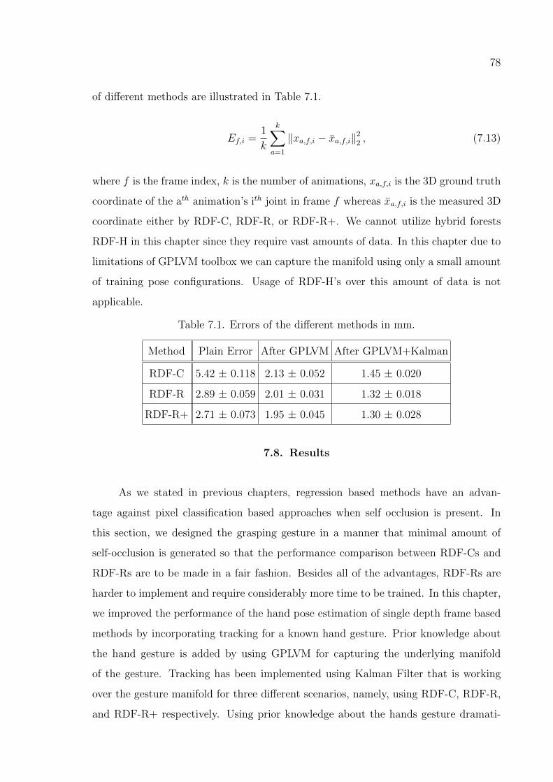
78
of different methods are illustrated in Table 7.1.
Ef,i =1
k
k∑a=1
‖xa,f,i − xa,f,i‖22 , (7.13)
where f is the frame index, k is the number of animations, xa,f,i is the 3D ground truth
coordinate of the ath animation’s ith joint in frame f whereas xa,f,i is the measured 3D
coordinate either by RDF-C, RDF-R, or RDF-R+. We cannot utilize hybrid forests
RDF-H in this chapter since they require vast amounts of data. In this chapter due to
limitations of GPLVM toolbox we can capture the manifold using only a small amount
of training pose configurations. Usage of RDF-H’s over this amount of data is not
applicable.
Table 7.1. Errors of the different methods in mm.
Method Plain Error After GPLVM After GPLVM+Kalman
RDF-C 5.42 ± 0.118 2.13 ± 0.052 1.45 ± 0.020
RDF-R 2.89 ± 0.059 2.01 ± 0.031 1.32 ± 0.018
RDF-R+ 2.71 ± 0.073 1.95 ± 0.045 1.30 ± 0.028
7.8. Results
As we stated in previous chapters, regression based methods have an advan-
tage against pixel classification based approaches when self occlusion is present. In
this section, we designed the grasping gesture in a manner that minimal amount of
self-occlusion is generated so that the performance comparison between RDF-Cs and
RDF-Rs are to be made in a fair fashion. Besides all of the advantages, RDF-Rs are
harder to implement and require considerably more time to be trained. In this chapter,
we improved the performance of the hand pose estimation of single depth frame based
methods by incorporating tracking for a known hand gesture. Prior knowledge about
the hand gesture is added by using GPLVM for capturing the underlying manifold
of the gesture. Tracking has been implemented using Kalman Filter that is working
over the gesture manifold for three different scenarios, namely, using RDF-C, RDF-R,
and RDF-R+ respectively. Using prior knowledge about the hands gesture dramati-
79
cally increases the performance of all methods as shown in Table 3.1. Employing a
Kalman Filter on top of GPLVM projection further enhances the results as expected.
Regression based methods RDF-R and RDF-R+ produce considerably better results
compared to RDF-Cs as expected. Although the gesture animation is designed in fa-
vor of having no self-occlusions, the animation contains the occlusion of the tip of the
thumb when the hand is fully closed. This is a major problem for RDF-Cs. They can-
not find the tip of the thumb which increases their error rate. However, RDF-Rs are
already known to produce better results when compared to RDF-Cs even without oc-
clusion, as demonstrated in this study in Section 6.2. Mean of the error improves from
5.42 mm to 2.71 mm. Standard deviation also improves in regression based methods.
An interesting result is that the standard deviation of RDF-R is better than RDF-R+.
This can also be reasonably explained by the error induced with the application of
dynamic programming. Dynamic programming of RDF-R+ method searches amount
different hand joint distributions for minimizing a penalty function. Penalty function is
a heuristic. A better penalty function may improve standard deviation performance of
RDF-R+. A dramatic improvement is achieved by using GPLVMs gesture manifold.
In the RDF-C case, the improvement is much greater than the improvement in the
regression based methods. This is also reasonable since RDF-Cs are known to be rela-
tively inaccurate compared to RDF-Rs. It is seen that the prior knowledge captured by
the gesture manifold corrects most of the inaccuracy of the RDF outputs. Fortunately
GPLVMs improvement still produces better performance on RDF-R and RDF-R+ as
expected. Consequently, Kalman Filter further enhances the mean and the variance of
the errors in both scenarios as well.
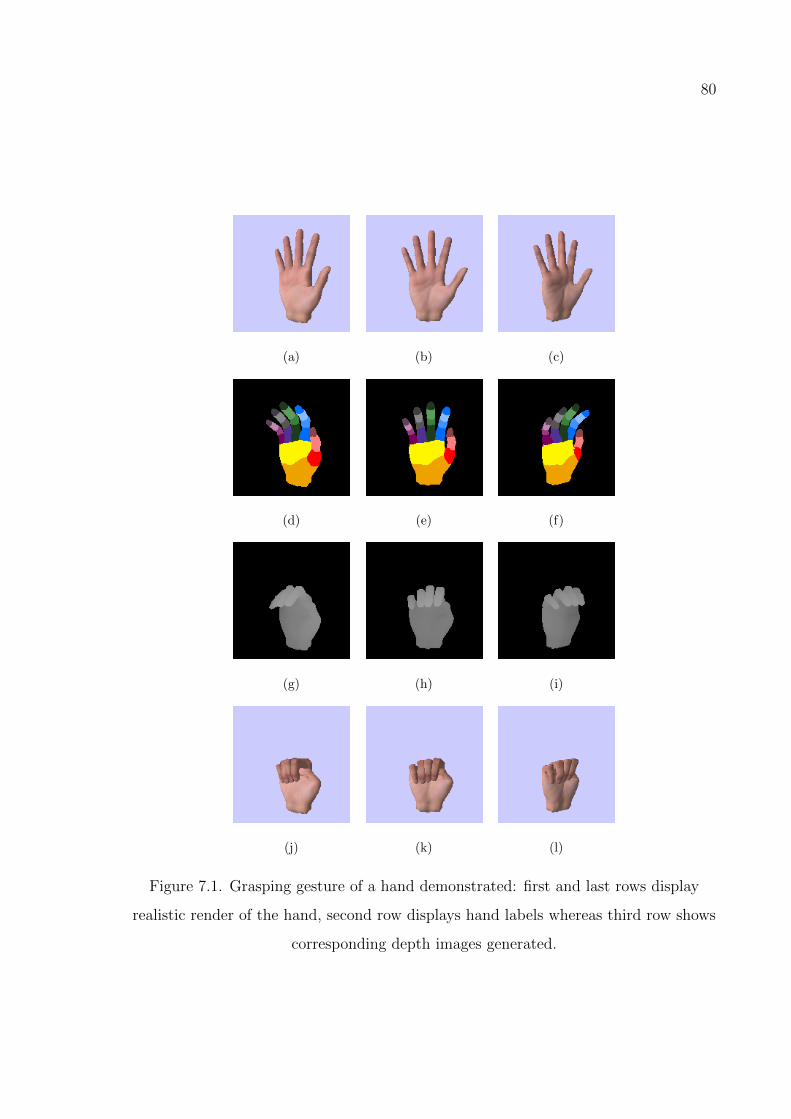
80
(a) (b) (c)
(d) (e) (f)
(g) (h) (i)
(j) (k) (l)
Figure 7.1. Grasping gesture of a hand demonstrated: first and last rows display
realistic render of the hand, second row displays hand labels whereas third row shows
corresponding depth images generated.
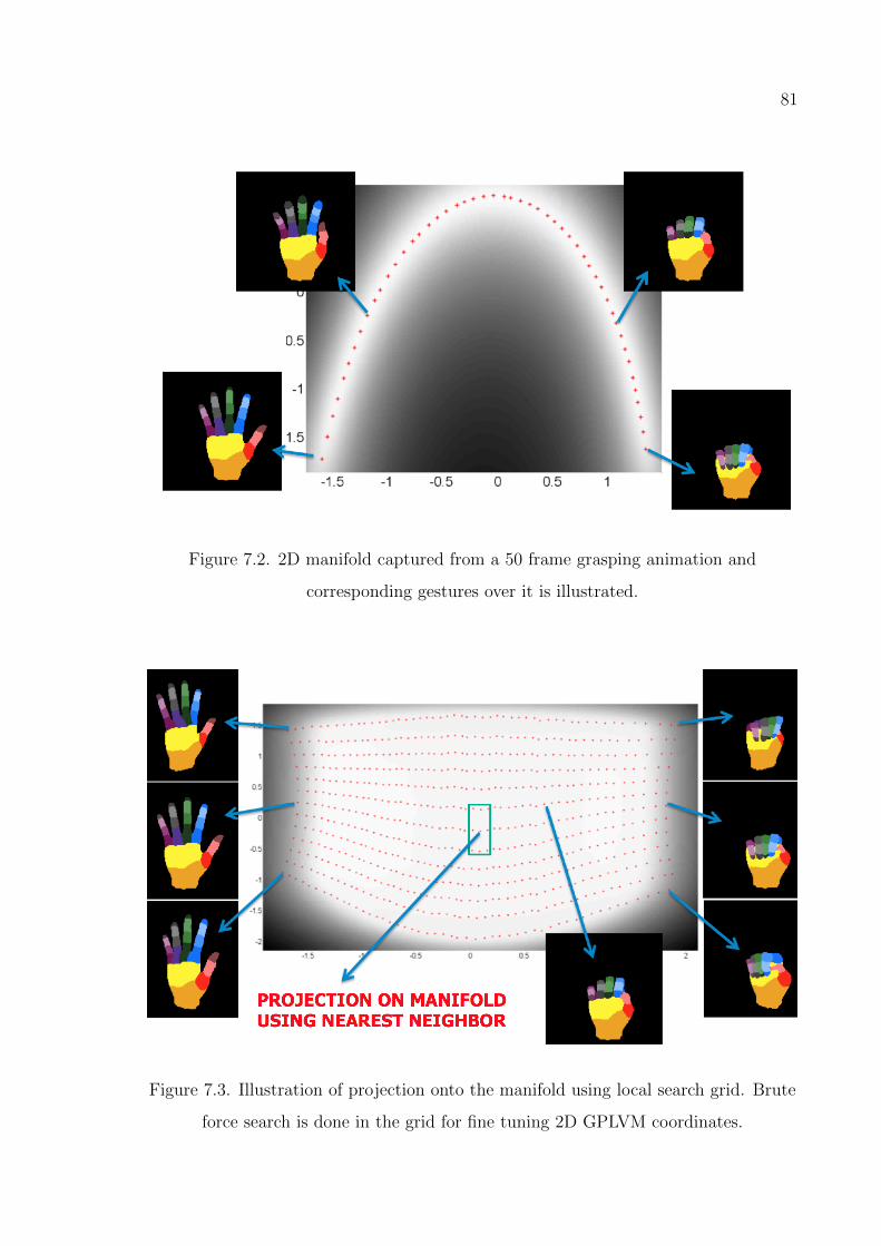
81
Figure 7.2. 2D manifold captured from a 50 frame grasping animation and
corresponding gestures over it is illustrated.
Figure 7.3. Illustration of projection onto the manifold using local search grid. Brute
force search is done in the grid for fine tuning 2D GPLVM coordinates.
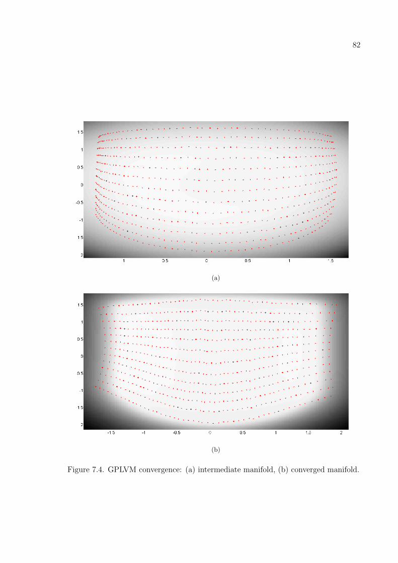
82
(a)
(b)
Figure 7.4. GPLVM convergence: (a) intermediate manifold, (b) converged manifold.
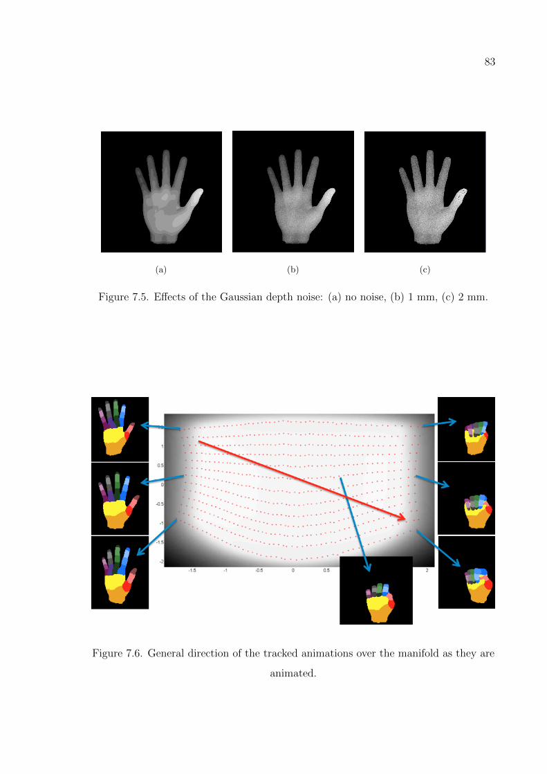
83
(a) (b) (c)
Figure 7.5. Effects of the Gaussian depth noise: (a) no noise, (b) 1 mm, (c) 2 mm.
Figure 7.6. General direction of the tracked animations over the manifold as they are
animated.
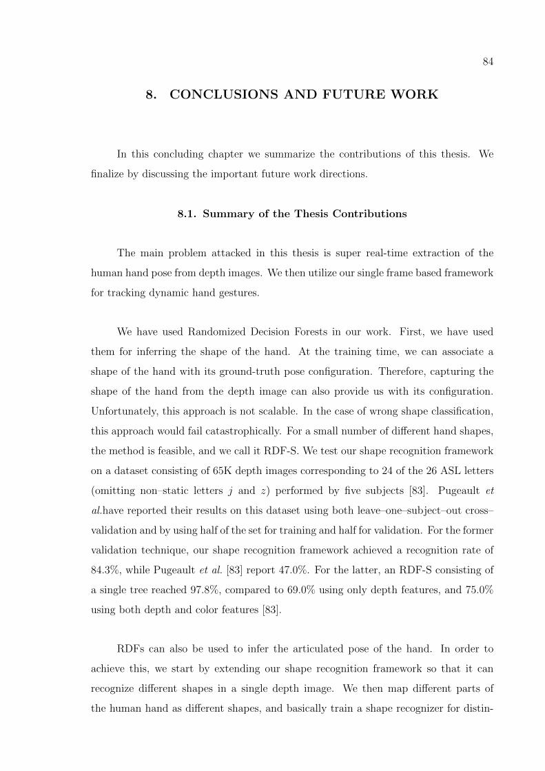
84
8. CONCLUSIONS AND FUTURE WORK
In this concluding chapter we summarize the contributions of this thesis. We
finalize by discussing the important future work directions.
8.1. Summary of the Thesis Contributions
The main problem attacked in this thesis is super real-time extraction of the
human hand pose from depth images. We then utilize our single frame based framework
for tracking dynamic hand gestures.
We have used Randomized Decision Forests in our work. First, we have used
them for inferring the shape of the hand. At the training time, we can associate a
shape of the hand with its ground-truth pose configuration. Therefore, capturing the
shape of the hand from the depth image can also provide us with its configuration.
Unfortunately, this approach is not scalable. In the case of wrong shape classification,
this approach would fail catastrophically. For a small number of different hand shapes,
the method is feasible, and we call it RDF-S. We test our shape recognition framework
on a dataset consisting of 65K depth images corresponding to 24 of the 26 ASL letters
(omitting non–static letters j and z) performed by five subjects [83]. Pugeault et
al.have reported their results on this dataset using both leave–one–subject–out cross–
validation and by using half of the set for training and half for validation. For the former
validation technique, our shape recognition framework achieved a recognition rate of
84.3%, while Pugeault et al. [83] report 47.0%. For the latter, an RDF-S consisting of
a single tree reached 97.8%, compared to 69.0% using only depth features, and 75.0%
using both depth and color features [83].
RDFs can also be used to infer the articulated pose of the hand. In order to
achieve this, we start by extending our shape recognition framework so that it can
recognize different shapes in a single depth image. We then map different parts of
the human hand as different shapes, and basically train a shape recognizer for distin-
85
guishing between different regions of the human hand, and call it RDF-C. Carefully
designing the regions, we assume the centroids of the different parts of the inferred
regions map to their corresponding hand joints. The centroids of the regions are found
by the mean shift mode finding algorithm. We choose mean shift due to its resistance
to outliers. The surface depth of the joint is acquired from the depth image, and the
correct 3D depth coordinate of the hand joint is evaluated by shifting the surface co-
ordinate by a predefined value. We assume this value for all of the human hand joints
to be constant.
We then combine our shape recognizer RDF-S and classification based pose es-
timator RDF-C for building a hybrid joint estimator, named as RDF-H. RDF-H uses
two layers of RDFs. In the first layer we utilize an RDF-S for choosing the cluster of
the hand pose. We then switch to an expert RDF-C which is specifically trained for
that cluster of the hand poses. Clustering the hand poses is done by employing spectral
clustering on the poses. RDF-H provides very good performance boost. It can improve
per pixel classification rates from 68.0% up to 91.2% in certain trials. Unfortunately,
RDF-Hs require vast amounts of data to be trained and are not suitable for small and
medium sized datasets.
RDF-Cs and RDF-Hs are basically designed for shape recognition in single depth
images. They are successful if the shapes are completely seen. In the case of the human
hand, the shapes are its different regions. These regions are prone to be invisible due
to self occlusion. The shape based methods are not adequate in the case of occlu-
sion. Unfortunately, the human hand is a very deformable object that produces self
occlusions all the time. For coping with this problem, we try to bypass the pixel classi-
fication phase and try to directly infer the joint coordinates. We incorporate regression
based approaches. We change the training and testing framework of our RDFs so that
they now do direct inference. We call this type of regression based RDFs as RDF-R.
RDF-Rs skip the pixel classification, hence, the shape recognition phase. They are
resistant to self occlusion by design. RDF-Rs, as expected, provide a great amount of
accuracy increase. However, all the methods we designed so far consider the different
joints of the hand as independent, which is clearly not the case. We try to incorporate
86
the hierarchical dependencies of different hand joints into our estimation process. We
call the new regression based method as RDF-R+. Fortunately, it further enhances
the accuracy [94].
We compare our different methods for joint estimation such as RDF-C, RDF-R,
RDF-R+. We carefully design different datasets for benchmarking their advantages
and disadvantages. RDF-R+ method achieves best accuracy performance both on
synthetic and real datasets.
As an additional improvement, we add temporal domain knowledge into the joint
estimation process by extracting a gesture manifold of the hand using GPLVM. We
run a Kalman tracker over the extracted manifold for successfully tracking a specific
grasping gesture of the hand. For the case of the grasping gesture, we achieve very
promising accuracy results. The best single image algorithm we designed, namely
RDF-R+, achieves 2.71 ± 0.073 mm average accuracy where manifold tracking method
achieves 1.30 ± 0.028 mm average accuracy.
8.2. Conclusions
Estimating the joint configuration of a very deformable object such as the human
hand is a tedious task. Most examples in the literature use exemplar-based approach.
Our shape recognition chapter, Chapter 4, describes a framework for exemplar-based
approach. Recognizing a specific hand shape inherently tells us about the pose con-
figuration. However, we further employ more sophisticated strategies for capturing
individual hand joint coordinates independently. Trying to estimate each joint on its
own comes with its advantages and disadvantages. As an advantage, this approach
is more generic. If a suitable learning scheme can be employed that can handle high
dimensionality without over-fitting the training data, this can be a great advantage.
Then we can generalize hand configurations as describing each and every different pose
of a human hand using exemplar-based methods is not feasible. Fortunately, random-
ized decision forests are known to be resistant to over-fitting. We also utilize their
massive parallelization potential for our super real-time speed target. These benefits
87
come with a big disadvantage that each joint is now independently estimated, hence,
losing the very valuable information of hierarchical constraints of our hand model.
Losing inter-dependencies of joints as we are gaining a more generic estimation
framework is a quality limiting bottleneck. Especially in the case of the human hand,
which can be captured in low resolutions due to limitations of the sensors, this approach
is prone to produce abnormal pose configurations from time to time. Extra constraints
must be imposed to the estimation layer which utilizes the hierarchical structure of the
model as we priorly know from the model. Our novel contribution RDF-R+ tries to
achieve that in a very fast manner without sacrificing from our super real-time speed
target. RDF-R+ guarantees to find a pose estimation which is compatible with the
bone lengths of the learned model. However it does impose a bone length constraint
blindly. The resulting skeleton, which is compatible with the model, can still not be
the combination of joints that are originally looked for.
A better approach would be to model the pose configurations that a human hand
can be in by extracting a low dimensional manifold. In Chapter 7, we both try to
learn the pose configuration manifold and track a specific dynamic hand gesture with
successful results. Learning the pose manifold using GPLVM is a tedious task. The
human hand pose configurations can easily generate a sample set of thousands of differ-
ent poses. GPLVM, a non-linear manifold extraction method, can generate qualitative
manifolds that can interpolate successfully between different training samples. Unfor-
tunately, there are two major drawbacks of GPLVM. First, its training phase takes
increasingly long times as we use thousands of different pose configurations for rep-
resenting the very complex hand pose configurations. Second, GPLVM learns only a
mapping from the reduced manifold space to the original pose space. Going from the
original pose space to the manifold space is not straightforward, though projecting the
poses to the extracted manifold provides very promising results. Due to our super
real-time aim, we test with a subset of the human hand poses with a very fast manifold
projection method in Chapter 7. Surprisingly we achieve promising results in a small
subset of gestures.
88
The framework is optimized for multi-core systems and is capable of running on
conventional notebooks without experiencing frame drops. Further enhancement is
possible through the utilization of the GPU, and this framework can be used along
with more CPU intensive applications such as games and modeling tools. Usage of
depth cameras has the extra benefit of not being affected by illumination also.
8.3. Directions for Future Works
8.3.1. Theoretical Investigation
A possibility for open theoretical research arises from the work presented here.
Jointly learning the underlying pose configuration manifold and the randomized forests
at the same time would be interesting. In our work, we were restricted in that fashion
due to manifold extraction’s high computational cost with our vast amount of training
samples.
Multi-layer hybrid approach showed us that combining different concepts in a
single architecture can boost the performance. In our case we utilized a shape recog-
nition layer preceding the original joint estimation phase and showed its performance
increase and better memory utilization. Combining two different trees actually pro-
duces another tree. We can further generalize this approach by looking at the hybrid
forests as a single forest whose different layers are optimized by different criteria. For
instance, training a single tree of depth 20, whose first 10 levels are trained using an
entropy gain objective for shapes and the last 10 layers with an entropy gain objec-
tive of specific joints is also an interesting way to investigate. Dynamically switching
between optimization criteria during training could be beneficial. More interestingly,
each layer’s optimization criterion can also be treated as a hyper-parameter.
Latent variable models (LVM) are valuable tools to investigate further. Recent
advances in LVMs provide incorporating constraints into the learning phase such as
in [95]. Non-linear dimensionality reduction area also has recent improvements as
presented by Geiger et al. [96]. Such works are a good direction for further investigation.
89
Physically-based motion models are also another area of recent research. As
the computational power increases we are able to design better but more complex
problems. State-of-the-art computer graphics hand models are using muscle models.
They model the physics of the muscles and animate the model by applying necessary
forces to the underlying muscles. This gives better interaction of the model with its
environment during a grasping or collision scenario. An interesting work concentrating
on 3D tracking combined with kinematic models is presented in [97].
8.3.2. Evaluation
We believe that a number of interesting additional experiments would be useful to
better understand the differences between algorithms and the conditions under which
each algorithm is best applicable. Such experiments include an evaluation of hybrid
forests more thoroughly. An investigation about different manifold extraction methods
is also needed. GPLVM is a state-of-the-art tool for non-linear manifolds recently.
However there are newer methods for classification and regression such as [98] and [96].
We investigated the performance of RDF-Hs comparatively with RDF-Cs in Sec-
tion 5.2. However both RDF-Cs and therefore RDF-Hs are not resistant to self-
occlusion. Another research area for performance evaluation can be combining the
power of hybrid forests with regression based methods.
Another aspect of empirical evaluation that should be improved is in the area of
comparing pose estimation algorithms in the literature. Although lack of a standard
articulated pose benchmark with known ground truth (neither real images nor realistic
synthetic ones) makes this difficult, it is important to compare alternative approaches.
We tried to compare our results with the live Surrey dataset by manually labeling the
ground truth of a small subset of poses in Section 6.5.3. A more comprehensive live
benchmark is still needed.
90
REFERENCES
1. Oikonomidis, I., N. Kyriazis and A. A. Argyros, “Markerless and Efficient 26-dof
Hand Pose Recovery”, Asian Conference on Computer Vision, pp. 744–757, 2011.
2. Microsoft Corporation, Kinect for Xbox 360, RedmondWA,
http://www.xbox.com/en-US/kinect, 2011.
3. Shotton, J., A. Fitzgibbon, M. Cook, T. Sharp, M. Finocchio, R. Moore, A. Kip-
man and A. Blake, “Real-time Human Pose Recognition in Parts from Single Depth
Images”, Computer Society Conference on Computer Vision and Pattern Recogni-
tion, Vol. 2, p. 3, 2011.
4. Ho, T. K., “Random Decision Forests”, International Conference on Document
Analysis and Recognition, Vol. 1, pp. 278–282, IEEE, 1995.
5. Keskin, C., F. Kırac, Y. E. Kara and L. Akarun, “Real Time Hand Pose Estimation
Using Depth Sensors”, International Conference on Computer Vision Workshops ,
pp. 1228–1234, IEEE, 2011.
6. Shotton, J., T. Sharp, A. Kipman, A. Fitzgibbon, M. Finocchio, A. Blake, M. Cook
and R. Moore, “Real-time Human Pose Recognition In Parts from Single Depth
Images”, Communications of the ACM , Vol. 56, No. 1, pp. 116–124, 2013.
7. Catmull, E., “A System for Computer Generated Movies”, Proceedings of the ACM
Annual Conference, Vol. 1, pp. 422–431, ACM, 1972.
8. Lee, D., M. Glueck, A. Khan, E. Fiume and K. Jackson, “A Survey of Modeling and
Simulation of Skeletal Muscle”, ACM Transactions on Graphics , Vol. 28, No. 4,
pp. 1–12, 2009.
9. Heap, T. and D. Hogg, “3D Deformable Hand Models”, Gesture Workshop, Vol. 13,
91
pp. 131–139, 1996.
10. Lin, J., Y. Wu and T. S. Huang, “Modeling the Constraints of Human Hand
Motion”, Proceedings of Workshop on Human Motion, pp. 121–126, IEEE, 2000.
11. Badler, N. I. and M. Morris, “Modelling Flexible Articulated Objects”, Proceedings
of Online Conference on Computer Graphics , pp. 305–314, 1982.
12. Magnenat-Thalmann, N., R. Laperrire, D. Thalmann et al., “Joint-dependent
Local Deformations for Hand Animation and Object Grasping”, Proceedings on
Graphics Interface, 1988.
13. Rijpkema, H. and M. Girard, “Computer Animation of Knowledge-based Human
Grasping”, SIGGRAPH Computer Graphics , Vol. 25, No. 4, pp. 339–348, 1991.
14. Gourret, J.-P., N. M. Thalmann and D. Thalmann, “Simulation of Object and
Human Skin Formations in A Grasping Task”, SIGGRAPH Computer Graphics ,
Vol. 23, pp. 21–30, ACM, 1989.
15. Foley, J. D., Computer Graphics: Principles and practice, in C , Vol. 12110,
Addison-Wesley Professional, 1996.
16. Cooney, W. P., M. J. Lucca, E. Chao and R. Linscheid, “The Kinesiology of the
Thumb Trapeziometacarpal Joint”, J Bone Joint Surg Am, Vol. 63, No. 9, pp.
1371–81, 1981.
17. Buford Jr, W. L., L. M. Myers and A. Hollister, “3-D Computer Graphics Simula-
tion of Thumb Joint Kinematics”, International Conference of the Engineering in
Medicine and Biology Society , pp. 833–834, IEEE, 1989.
18. Thompson, D. E., W. L. Buford Jr, L. M. Myers, D. J. Giurintano and J. A.
Brewer III, “A Hand Biomechanics Workstation”, SIGGRAPH Computer Graph-
ics , Vol. 22, pp. 335–343, ACM, 1988.
92
19. Albrecht, I., J. Haber and H. Seidel, “Construction and Animation of Anatomically
Based Human Hand Models”, Eurographics/SIGGRAPH Symposium on Computer
Animation, 2003.
20. Thalmann, N. M. and D. Thalmann, “Hidden Surfaces, Reflectance, and Shading”,
Computer Animation, pp. 87–99, Springer, 1990.
21. Deutscher, J., A. Blake and I. Reid, “Articulated Body Motion Capture by An-
nealed Particle Filtering”, Proceedings of the Computer Vision and Pattern Recog-
nition, Vol. 2, pp. 126–133, IEEE, 2000.
22. Pavlovic, V. I., R. Sharma and T. S. Huang, “Visual Interpretation of Hand Ges-
tures for Human-computer Interaction: A Review”, Transactions on Pattern Anal-
ysis and Machine Intelligence, Vol. 19, No. 7, pp. 677–695, 1997.
23. Torus Knot Software, Ogre3D (Version 1.8.1), http://www.ogre3d.org/.
24. Girshick, R., J. Shotton, P. Kohli, A. Criminisi and A. Fitzgibbon, “Efficient Re-
gression of General-activity Human Poses from Depth Images”, International Con-
ference on Computer Vision, pp. 415–422, IEEE, 2011.
25. Fergus, R., P. Perona and A. Zisserman, “Object Class Recognition by Unsuper-
vised Scale-invariant Learning”, Computer Society Conference on Computer Vision
and Pattern Recognition, Vol. 2, pp. II–264, IEEE, 2003.
26. Winn, J. and J. Shotton, “The Layout Consistent Random Field for Recognizing
and Segmenting Partially Occluded Objects”, Computer Society Conference on
Computer Vision and Pattern Recognition, Vol. 1, pp. 37–44, IEEE, 2006.
27. Liu, X. and K. Fujimura, “Hand Gesture Recognition Using Depth Data”, Interna-
tional Conference on Automatic Face and Gesture Recognition, pp. 529–534, IEEE,
2004.
28. Grest, D., J. Woetzel and R. Koch, “Nonlinear Body Pose Estimation from Depth
93
Images”, Pattern Recognition, pp. 285–292, Springer, 2005.
29. Knoop, S., S. Vacek and R. Dillmann, “Sensor Fusion for 3d Human Body Tracking
with An Articulated 3d Body Model”, International Conference on Robotics and
Automation, pp. 1686–1691, IEEE, 2006.
30. Zhu, Y. and K. Fujimura, “Constrained Optimization for Human Pose Estima-
tion from Depth Sequences”, Asian Conference on Computer Vision, pp. 408–418,
Springer, 2007.
31. Bourdev, L. and J. Malik, “Poselets: Body Part Detectors Trained Using 3d Human
Pose Annotations”, International Conference on Computer Vision, pp. 1365–1372,
IEEE, 2009.
32. Siddiqui, M. and G. Medioni, “Human Pose Estimation from A Single View Point,
Real-time Range Sensor”, Computer Society Conference on Computer Vision and
Pattern Recognition Workshops , pp. 1–8, IEEE, 2010.
33. Plagemann, C., V. Ganapathi, D. Koller and S. Thrun, “Real-time Identification
and Localization of Body Parts from Depth Images”, International Conference on
Robotics and Automation, pp. 3108–3113, IEEE, 2010.
34. Ganapathi, V., C. Plagemann, D. Koller and S. Thrun, “Real Time Motion Cap-
ture Using A Single Time-of-flight Camera”, Conference on Computer Vision and
Pattern Recognition, pp. 755–762, IEEE, 2010.
35. Suryanarayan, P., A. Subramanian and D. Mandalapu, “Dynamic Hand Pose
Recognition Using Depth Data”, International Conference on Pattern Recognition,
pp. 3105–3108, IEEE, 2010.
36. Doliotis, P., V. Athitsos, D. Kosmopoulos and S. Perantonis, “Hand Shape and 3d
Pose Estimation Using Depth Data From A Single Cluttered Frame”, Advances in
Visual Computing , pp. 148–158, Springer, 2012.
94
37. Gallo, L. and A. P. Placitelli, “View-independent Hand Posture Recognition from
Single Depth Images Using PCA and Flusser Moments”, Signal Image Technology
and Internet Based Systems (SITIS), Eighth International Conference on, pp. 898–
904, IEEE, 2012.
38. Billiet, L., M. Oramas, M. Hoffmann, W. Meert, L. Antanas et al., “Rule-based
Hand Posture Recognition Using Qualitative Finger Configurations Acquired with
The Kinect”, Proceedings of the 2nd International Conference on Pattern Recog-
nition Applications and Methods , pp. 1–4, 2013.
39. Yao, Y. and Y. Fu, “Real-time Hand Pose Estimation from RGB-D Sensor”, In-
ternational Conference on Multimedia and Expo, pp. 705–710, IEEE, 2012.
40. Liang, H., J. Yuan and D. Thalmann, “Hand Pose Estimation by Combining Fin-
gertip Tracking And Articulated ICP”, Proceedings of the 11th ACM SIGGRAPH
International Conference on Virtual-Reality Continuum and its Applications in
Industry , pp. 87–90, ACM, 2012.
41. Breiman, L., “Random Forests”, Machine learning , Vol. 45, No. 1, pp. 5–32, 2001.
42. Ye, M., X. Wang, R. Yang, L. Ren and M. Pollefeys, “Accurate 3d Pose Estimation
from A Single Depth Image”, International Conference on Computer Vision, pp.
731–738, IEEE, 2011.
43. Lopez-Mendez, A., M. Alcoverro, M. Pardas and J. R. Casas, “Real-time Upper
Body Tracking with Online Initialization Using A Range Sensor”, International
Conference on Computer Vision Workshops , pp. 391–398, IEEE, 2011.
44. Bregler, C. and J. Malik, “Tracking People With Twists and Exponential Maps”,
Computer Society Conference on Computer Vision and Pattern Recognition, pp.
8–15, IEEE, 1998.
45. Sigal, L., S. Bhatia, S. Roth, M. J. Black and M. Isard, “Tracking Loose-limbed
95
People”, Computer Society Conference on Computer Vision and Pattern Recogni-
tion, Vol. 1, pp. I–421, IEEE, 2004.
46. Wang, R. Y. and J. Popovic, “Real-time Hand-tracking with A Color Glove”,
Transactions on Graphics , Vol. 28, p. 63, ACM, 2009.
47. Brubaker, M. A., D. J. Fleet and A. Hertzmann, “Physics-based Person Tracking
Using the Anthropomorphic Walker”, International Journal of Computer Vision,
Vol. 87, No. 1-2, pp. 140–155, 2010.
48. Erol, A., G. Bebis, M. Nicolescu, R. D. Boyle and X. Twombly, “Vision-based
Hand Pose Estimation: A Review”, Computer Vision and Image Understanding ,
Vol. 108, No. 1, pp. 52–73, 2007.
49. Suarez, J. and R. R. Murphy, “Hand Gesture Recognition with Depth Images: A
Review”, RO-MAN , pp. 411–417, IEEE, 2012.
50. Athitsos, V. and S. Sclaroff, “Estimating 3d Hand Pose from A Cluttered Image”,
Computer Society Conference on Computer Vision and Pattern Recognition, Vol. 2,
pp. II–432, IEEE, 2003.
51. de Campos, T. E. and D. W. Murray, “Regression-based Hand Pose Estimation
from Multiple Cameras”, Computer Society Conference on Computer Vision and
Pattern Recognition, Vol. 1, pp. 782–789, IEEE, 2006.
52. de La Gorce, M., D. J. Fleet and N. Paragios, “Model-based 3d Hand Pose Es-
timation from Monocular Video”, Transactions on Pattern Analysis and Machine
Intelligence, Vol. 33, No. 9, pp. 1793–1805, 2011.
53. Thippur, A., C. H. Ek and H. Kjellstrom, “Inferring Hand Pose: A Comparative
Study of Visual Shape Features”, International Conference on Face and Gesture,
2013.
54. Singh, V. K. and R. Nevatia, “Action Recognition in Cluttered Dynamic Scenes
96
Using Pose-specific Part Models”, International Conference on Computer Vision,
pp. 113–120, IEEE, 2011.
55. Stenger, B., P. R. Mendonca and R. Cipolla, “Model-based 3d Tracking of An Ar-
ticulated Hand”, Conference on Computer Vision and Pattern Recognition, Vol. 2,
pp. II–310–II–315, IEEE, 2001.
56. Rosales, R., V. Athitsos, L. Sigal and S. Sclaroff, “3d Hand Pose Reconstruction
Using Specialized Mappings”, Proceedings of the Eighth IEEE International Con-
ference on Computer Vision, Vol. 1, pp. 378–385, IEEE, 2001.
57. Virtual Technologies, VirtualHand Software Library Reference Manual,
http://www.scribd.com/doc/100401915/Virtual-Hand, 1998.
58. Mo, Z. and U. Neumann, “Real-time Hand Pose Recognition Using Low-resolution
Depth Images”, Computer Society Conference on Computer Vision and Pattern
Recognition, Vol. 2, pp. 1499–1505, IEEE, 2006.
59. Malassiotis, S. and M. G. Strintzis, “Real-time Hand Posture Recognition Using
Range Data”, Image and Vision Computing , Vol. 26, No. 7, pp. 1027–1037, 2008.
60. Keskin, C., F. Kırac, Y. E. Kara and L. Akarun, “Multilayered Randomized Clas-
sification Forests for Hand Pose Estimation Using Depth Sensors ”, International
Conference on Computer Vision and Pattern Recognition Workshops on Gesture
Recognition, Springer, 2012.
61. Ong, E.-J. and R. Bowden, “A Boosted Classifier Tree for Hand Shape Detection”,
International Conference on Automatic Face and Gesture Recognition, pp. 889–
894, IEEE, 2004.
62. Keskin, C., F. Kırac, Y. E. Kara and L. Akarun, “Hand Pose Estimation and Hand
Shape Classification Using Multi-layered Randomized Decision Forests”, European
Conference on Computer Vision, pp. 852–863, Springer, 2012.
97
63. MacKay, D. J., “Bayesian Neural Networks and Density Networks”, Nuclear In-
struments and Methods in Physics Research Section A: Accelerators, Spectrometers,
Detectors and Associated Equipment , Vol. 354, No. 1, pp. 73–80, 1995.
64. Bishop, C. M., M. Svensen and C. K. Williams, “GTM: A Principled Alternative to
The Self-organizing Map”, International Conference on Artificial Neural Networks ,
pp. 165–170, Springer, 1996.
65. Bishop, C. M., M. Svensen and C. K. Williams, “GTM: The Generative Topo-
graphic Mapping”, Neural Computation, Vol. 10, No. 1, pp. 215–234, 1998.
66. Kohonen, T., “The Self-organizing Map”, Proceedings of the IEEE , Vol. 78, No. 9,
pp. 1464–1480, 1990.
67. Tipping, M. E. and C. M. Bishop, “Probabilistic Principal Component Analysis”,
Journal of the Royal Statistical Society: Series B (Statistical Methodology), Vol. 61,
No. 3, pp. 611–622, 1999.
68. Tenenbaum, J. B., V. De Silva and J. C. Langford, “A Global Geometric Frame-
work for Nonlinear Dimensionality Reduction”, Science, Vol. 290, No. 5500, pp.
2319–2323, 2000.
69. Shi, J. and J. Malik, “Normalized Cuts and Image Segmentation”, Transactions
on Pattern Analysis and Machine Intelligence, Vol. 22, No. 8, pp. 888–905, 2000.
70. Elgammal, A. and C.-S. Lee, “Inferring 3d Body Pose from Silhouettes Using
Activity Manifold Learning”, Computer Society Conference on Computer Vision
and Pattern Recognition, Vol. 2, pp. II–681, IEEE, 2004.
71. Grochow, K., S. L. Martin, A. Hertzmann and Z. Popovic, “Style-based Inverse
Kinematics”, ACM Transactions on Graphics , Vol. 23, pp. 522–531, ACM, 2004.
72. Lawrence, N., “Probabilistic Non-linear Principal Component Analysis with Gaus-
sian Process Latent Variable Models”, The Journal of Machine Learning Research,
98
Vol. 6, pp. 1783–1816, 2005.
73. Teh, Y. W. and S. T. Roweis, “Automatic Alignment of Local Representations”,
Advances in Neural Information Processing Systems , pp. 841–848, 2002.
74. Sminchisescu, C. and A. Jepson, “Generative Modeling for Continuous Non-linearly
Embedded Visual Inference”, Proceedings of the 21st International Conference on
Machine Learning , p. 96, ACM, 2004.
75. Urtasun, R., D. J. Fleet, A. Hertzmann and P. Fua, “Priors for People Tracking
from Small Training Sets”, International Conference on Computer Vision, Vol. 1,
pp. 403–410, IEEE, 2005.
76. Wang, J. M., D. J. Fleet and A. Hertzmann, “Gaussian Process Dynamical Models
for Human Motion”, Transactions on Pattern Analysis and Machine Intelligence,
Vol. 30, No. 2, pp. 283–298, 2008.
77. Urtasun, R., D. J. Fleet and P. Fua, “3d People Tracking with Gaussian Pro-
cess Dynamical Models”, Computer Society Conference on Computer Vision and
Pattern Recognition, Vol. 1, pp. 238–245, IEEE, 2006.
78. Moon, K. and V. Pavlovic, “Impact of Dynamics on Subspace Embedding and
Tracking of Sequences”, Computer Society Conference on Computer Vision and
Pattern Recognition, Vol. 1, pp. 198–205, IEEE, 2006.
79. Tian, T.-P., R. Li and S. Sclaroff, Tracking Human Body Pose on A Learned Smooth
Space, Tech. rep., Boston University Computer Science Department, 2005.
80. Li, R., M.-H. Yang, S. Sclaroff and T.-P. Tian, “Monocular Tracking of 3d Human
Motion with A Coordinated Mixture of Factor Analyzers”, European Conference
on Computer Vision, pp. 137–150, Springer, 2006.
81. Ek, C. H., P. H. S. Torr and N. D. Lawrence, “Gaussian Process Latent Variable
Models for Human Pose Estimation”, Proceedings of the 4th International Con-
99
ference on Machine Learning for Multimodal Interaction, pp. 132–143, Springer-
Verlag, 2008.
82. Lee, C.-S., S. Y. Chun and S. W. Park, “Articulated Hand Configuration and Ro-
tation Estimation Using Extended Torus Manifold Embedding”, 21st International
Conference on Pattern Recognition, pp. 441–444, IEEE, 2012.
83. Pugeault, N. and R. Bowden, “Spelling It Out: Real-time ASL Fingerspelling
Recognition”, International Conference on Computer Vision Workshops , pp. 1114–
1119, IEEE, 2011.
84. Uebersax, D., J. Gall, M. Van den Bergh and L. Van Gool, “Real-time Sign Lan-
guage Letter and Word Recognition from Depth Data”, International Conference
on Computer Vision Workshops , pp. 383–390, IEEE, 2011.
85. Comaniciu, D. and P. Meer, “Mean Shift: A Robust Approach Toward Fea-
ture Space Analysis”, Transactions on Pattern Analysis and Machine Intelligence,
Vol. 24, No. 5, pp. 603–619, 2002.
86. Shi, J. and J. Malik, “Normalized Cuts and Image Segmentation”, Conference on
Computer Vision and Pattern Recognition, p. 731, Washington, DC, USA, 1997.
87. Meila, M. and J. Shi, “A Random Walks View of Spectral Segmentation”, AI and
Statistics , 2001.
88. Vitter, J. S., “Random Sampling with A Reservoir”, ACM Transactions on Math-
ematical Software, Vol. 11, No. 1, pp. 37–57, 1985.
89. Kass, S., “Rock Paper Scissors Spock Lizard Game”,
http://www.samkass.com/theories/RPSSL.html, 1995.
90. Guyon, I., V. Athitsos, P. Jangyodsuk, B. Hamner and H. J. Escalante, “Chalearn
Gesture Challenge: Design and First Results”, Computer Society Conference on
Computer Vision and Pattern Recognition Workshops , pp. 1–6, IEEE, 2012.
100
91. Rasmussen, C. E. and C. K. Williams, Gaussian Processes for Machine Learning ,
The MIT Press, 2006.
92. Lawrence, N. D. and J. Quinonero-Candela, “Local Distance Preservation in The
GP-LVM Through Back Constraints”, Proceedings of the 23rd International Con-
ference on Machine Learning , pp. 513–520, ACM, 2006.
93. Quirion, S., C. Duchesne, D. Laurendeau and M. Marchand, “Comparing GPLVM
Approaches for Dimensionality Reduction in Character Animation”, Journal of
WSCG., Vol. 16, No. 1–3, pp. 41–48, 2008.
94. Kırac, F., Y. E. Kara and L. Akarun, “Hierarchically Constrained 3D Hand Pose
Estimation Using Regression Forests from Single Frame Depth Data”, Pattern
Recognition Letters Special Issue on Depth Image Analysis , 2013.
95. Varol, A., M. Salzmann, P. Fua and R. Urtasun, “A Constrained Latent Variable
Model”, Conference on Computer Vision and Pattern Recognition, pp. 2248–2255,
IEEE, 2012.
96. Geiger, A., R. Urtasun and T. Darrell, “Rank Priors for Continuous Non-linear
Dimensionality Reduction”, Conference on Computer Vision and Pattern Recog-
nition, pp. 880–887, IEEE, 2009.
97. Salzmann, M. and R. Urtasun, “Physically-based Motion Models for 3d Tracking:
A Convex Formulation”, International Conference on Computer Vision, pp. 2064–
2071, IEEE, 2011.
98. Urtasun, R. and T. Darrell, “Discriminative Gaussian Process Latent Variable
Model for Classification”, Proceedings of the 24th International Conference on Ma-
chine Learning , pp. 927–934, ACM, 2007.


![Vision-Based Relative Pose Estimation for Autonomous ... · tion [4], template matching [9], contour tracking [8], and ar-ticulated object tracking [11]. Model-Based Pose Estimation](https://img.pdfslide.net/doc/110x75/60096d0eeb4bb91006635959/vision-based-relative-pose-estimation-for-autonomous-tion-4-template-matching.jpg)