Real-time operational control of flexible manufacturing systems

Real-time Operational Control of Flexible Manufactm'ing Systems

Oded Z. Maimon, Tel Aviv University, Tel Aviv, Israel

Abstract

This paper provides a real-time operational control detailed scheme for flexible manufacturing systems. The control is organized in a hierarchical structure according to the various decisions that take place at the different time scales at which each level operates, from a few days to milliseconds.

At each level down the hierarchy, the details of the decisions and the communication rate increase. Feedback laws are developed to optimally take into account the real-time status of the system at each level. The highest real- time level accepts short-term management production requirements and the lowest level issues commands to the direct machine controllers. The control actions range from determining the changing product mix and input f low rate, through in-process parts movement decisions, to resource allocation in order to perform these moves in an efficient, conflict-free manner. Each level issues target commands to the level below and receives performance feedback. The overall control aims to optimize FMS per- f o rmance w h i l e meet ing the p roduc t ion requirements.

Models for each level and the interaction among the levels are presented and demon- strated via a case study. A previous version of the controller is currently used to control and run some experimental and industrial systems.

Keywords." FMS, Computer Integrated Manufacturing, Operational Control, Real- Time.

Introduction

This paper presents a method of controlling the short-term activities in a flexible manufacturing system. The input to the controller is the short-term production requirement (e.g., a few days), and system status. The outputs are commands to the direct machine controller to execute particular moves or a program.

An FMS consists of a set of machines, a material handling system (MHS) and information system, and service centers all working together toward a common production goal.

In addition, an FMS is characterized by the versatility of its components (see, for example, Ref- erence I for a general survey of FM S). Workstations (e.g., robots, NC machines) are capable of perform- ing many different operations, given the proper tooling, fixtures, and materials. Another feature is the short switching time between different operations assigned to a workstation (among a family of operations), ~ for example, downloading of an NC program. The MHS can be directed via different routes, to various destinations, carrying a variety of loads.

In manufacturing, hardware and software that automatically carry out particular tasks are well developed and in existence. However, even with adequate automation equipment, the manufacturing, as a system, usually does not live up to its performance potential. One main reason for this

125

Journal of Manufacturing Systems Volume 6/No. 2

phenomenon is the lack of appropriate integratio and control of the FMS operation.

Operational control of an FMS is very compli- cated. It involves accessing large static and dynamic data sets (representing machine configuration and characteristics, system status, and process plans), and complex control algorithms. The control algorithms are structured hierarchically, where an upper level issues commands to a lower level and gets feedback on the achievement of these commands.

Some other manufacturing issues that are dealt with in manufacturing software are found in Refer- ence 3. They include cost estimation, employee production efficiency, response to changes, and various types of report generation. Other related issues are those that are usually planned beyond the daily operations such as layout design, 4 capacity and production planning: and lot sizing. 6.,4

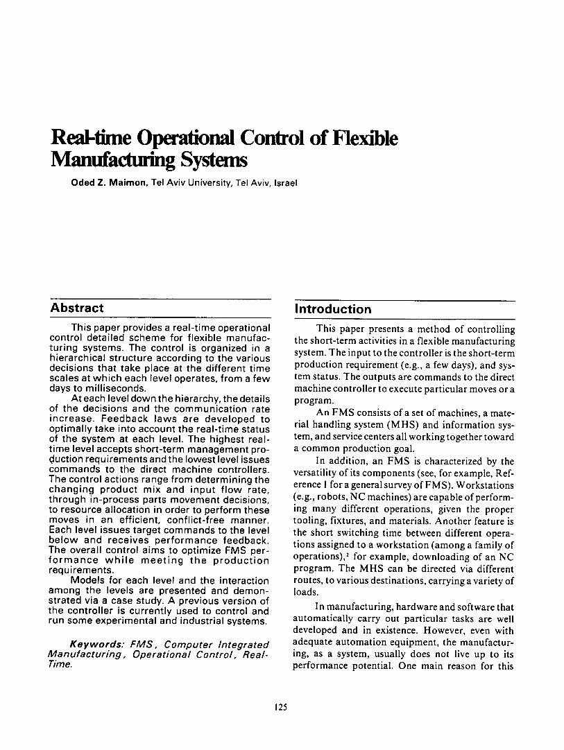
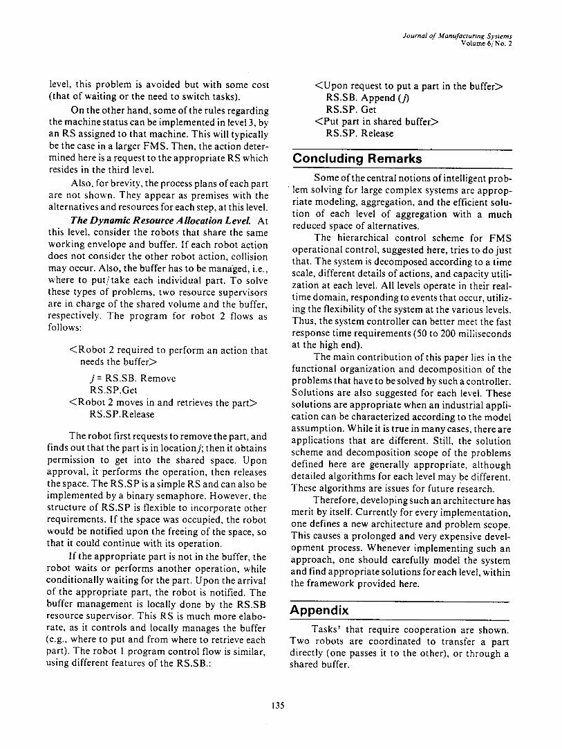
The contribution of this paper lies in the development of a generic hierarchical control system, depicted in Figure 1, to carry out the FMS integration from the production requirements to the actual operation of the machines. Reference to some exist- ing stand-alone components are given later. A previous version of the controller presented here was success fu l ly i m p l e m e n t e d , as d e s c r i b e d by Maimon 7.s (pictures of the system in operation are shown in the Appendix).

Different levels of the control operate at different time scales and determine different operational decisions, from aggregated parameters to more detailed ones. Thus, the control system can effi- ciently handle the enormous amount of static and dynamic data and decisions required to automatically operate a complex system, such as an FMS.

The system depicted in Figure 1 is divided into user interface, databases, a control part, and communication. Via manufacturing input language, the user enters the system representation to the various databases. Two major databases define the manufacturing system and the processes. Merging the two results in alternative process plans for a particular FMS type3

The FMS control part consists of three levels. The first level is the dynamic scheduler/.'* which determines the instantaneous production rate of each part type to best utilize the varying capacity of the system. The process sequencer level determines the details of the internal movement of par ts : . " To

e3

C3

I User Interface Management (& Monitoring; Reports; Statistics) "~ ~ r--

Configuration D.B.

World Status (Real-Time)

Short-Term Requirements

D.B

(Alternative) Resources

& Spatial Process Optimization

O

o

d

Loca I Area Networ

Performance Criteria

Inst. Prod. Rate j~ Route Split

Dispatcher

I 7 I Process Sequencer

I 1 I Dynamic

Resource Allocator (Conflict Avoidance)

I Run-Time Services (Status Updates; Data Collection 1 Communication Post-Processor

t

~Automated I ~ lU l Modules I ~ I F~ - ° -

Figure ! Flexible Manufacturing System Controller Scheme

cut the number of possibilities to evaluate at this level, some of the interdependent conflicts are solved at a lower level by a faster mechanism to determine the timing of the machine operation3."

Finally, the communicat ion leveW .'6 transmits the decisions and receives feedback from the direct machine controllers. Part of this level is also in charge of collecting statistical data, monitoring options of the system, and providing run time services. An event processor coordinates the overall activities in the controller.

Next, the three control levels are concentrated on and their operation and integration are demon- strated via a case study.

Note that the dynamic scheduling considered at the various levels here, to satisfy the FMS control and automatic operation requirement, is different from the traditional scheduling," before FMSs emerged. The main difference is in the in-time response to real-time events and the utilization of

126


the manufacturing system's flexibility. Classical scheduling is mostly interested in the static case, where all the machines, jobs and their precedence relations are given in advance. Also, they do not deal with the low level operational details such as collision avoidance, an issue which has to be addressed in the dynamic manufacturing environment and the new technology (such as robotics) being considered now.

The Control Levels T h e S c h e d u l e r L e v e l This is the first level of

the hierarchical controller. This level determines which part to produce next and via which preferable route. This level includes three types of decisions:

1. Part type's instantaneous production rate. 2. Planned routing. 3. Part dispatch timing.

This level's goal is to achieve the short-term production demand, while keeping work-in-process inventory as small as possible and optimally utilizing the system capacity. Real-time knowledge of some events that occur (e.g., machine failure) is required to define the changing system capacity. This knowledge is taken into account in a closed feedback loop, and by modeling the capacity as a stochastic process, reflecting resources availability behavior. That is, when determining the instantaneous production rate, possible future machine failures are considered.

Other considerat ions of this level are the priorities among competing part types. The priority scheme has static and dynamic parts. The static priorities are based on the relative importance of the various part types to be manufactured. The dynamic priorities are based on the cumulative production goals achieved at any point in time.

For example, part type b may be more impor- tant than part type c. If the cumulative production ofb is close to its goal (at time t), while c is far behind (at t), then from this point of time until c catches up with its goal, part type c may be preferred when a decision between dispatching a part of type b or c has to be made.

To carry out these ideas, the system at this level is modeled as follows:

1. Production surplus state, x:

(t) = u(t) - d

where, d is the vector of demand rate, and u( t ) represents the instantaneous production rate (IPR).

For the given product ion requirements, D(T), for the short-term horizon T, let:

d = T-' D(T).

Note that vector notation is used, and that the vectors are of magnitude n, the number of the different part types considered for production in the FMS. Definey * as the IPR of route k, where route is defined as the sequence of machines that a part has to follow until its production is completed. Multiple visits to a machine are allowed.

Let u(t) = Y~ ky*( t ) .

2. Resource state model:

P(ot(t + 6 0 =j /or ( t ) = 0 = Xqd t

where: a (t) denotes the number of available machines at time t.

The above states that the probability of having j resources available at time (t + 6 t), given that there were i resources available at t, is h ;i 6 t, plus a small negligent value. The matrix, whose elements are hai i,j, = 0 ..... m , where m is the number of machine types, is called the generator transformation matrix.

This assumption and others, which lead to a Poisson Process, have been tested (in some environ- ments) and proven appropriate to model the process of machine failures and repairs. Note also that to implement it, only two characteristics of a machine are required, namely, MTBF (mean time between failure) and MTTR (mean time to repair), h ii = M T B F " or M T T R ~ for a machine to fail or to be repaired, if failed. This type of required data fits the philosophy of using less frequent aggregate data at higher levels of control.

3. Capacity modeling: Often in FMS few machines are required to

produce a part type. To describe the capacity of the FMS for a mix of parts (given the machines that are up and working at any point in time), a set is required that presents the various tradeoffs. Let fl (c~ (t)) denote the capacity set, then:

f l (or (t)) = {),*(t) " •, ~i, k ),~ T~i ~ o~ V j}

where T~i is the product ion time of part type i on machine j, if route k is considered, and a i is the number of available machines of type j.

127


4. Penalty function: The final component of the model is the

penalty function. It is used to assess the relative importance among the various part types. The penalty function is denoted by g(x(t)) . Typically, larger penalties are assigned for backlog (x < 0), then for being ahead (x>0). Determining the penalty values is the duty of the production supervisor who needs to understand the effects and consequences of these functions on the scheduler behavior.

At this point, we are prepared to rigorously formulate the problem at this level as (P):

y * (t) = argy~ n (a (t)) rain {Ef~ g ( x ( t ) ) d t / x , , oq}

y * (t) = arg min J ( x o, ot o)

The cost function J ( x o, s 0) reflects the relative operational performance of the FMS during the time interval (0, T), starting with initial conditions x, (typically equal to zero) and s 0. The cost is relative in terms of the preassigned g(.), and is just a mechanism to obtain the instantaneous production rate 0'*(t)), to best meet the FMS production goals while utilizing the capacity and reducing work-in- process inventory.

Note that this model assumes a fast switching time among the various part types of the family or part types assigned to the FMS. This is not always the case. Methods for modifying the model to take into account setup times and local inventories exist, but are not elaborated here (see Reference 14 for example).

The solution method 9 to obtain y * (t) is out- lined next. It is solved in three levels.

1. Approximate J by J, where:

j = ½ x r A ( a ) x + br(a)x + c(a)

A " n x n diagonal matrix

b = l xn vector

2. By dynamic programming, the solution to min,J(a,x) , is obtained by solving the following in real-time (state-dependent):

min 6 J(x,~_______~) y( t ) y ~ lq(a(t)) 8x(t)

3. From y(t) obtained above, determine which parts to actually dispatch to the system, based upon min t (x¢ - x~' ) (according to routes also), where:

x~ - x~ A c t u a l (surplus state of the system) P = x i Pro jec ted (from the calculated y) X i

That is, among the parts to be dispatched, the one furthest behind is dispatched first.

T h e P r o c e s s S e q u e n c e r L e v e L The system continues with more detailed decisions by knowing which part type should be produced next and via which preferred route.

Here, for each part type, the system determines the next process and move. Based on the manufacturing system status and the production state of the part, the process sequencer (PS) infers the next process, the appropriate material handling move, and the production program to download, if required.

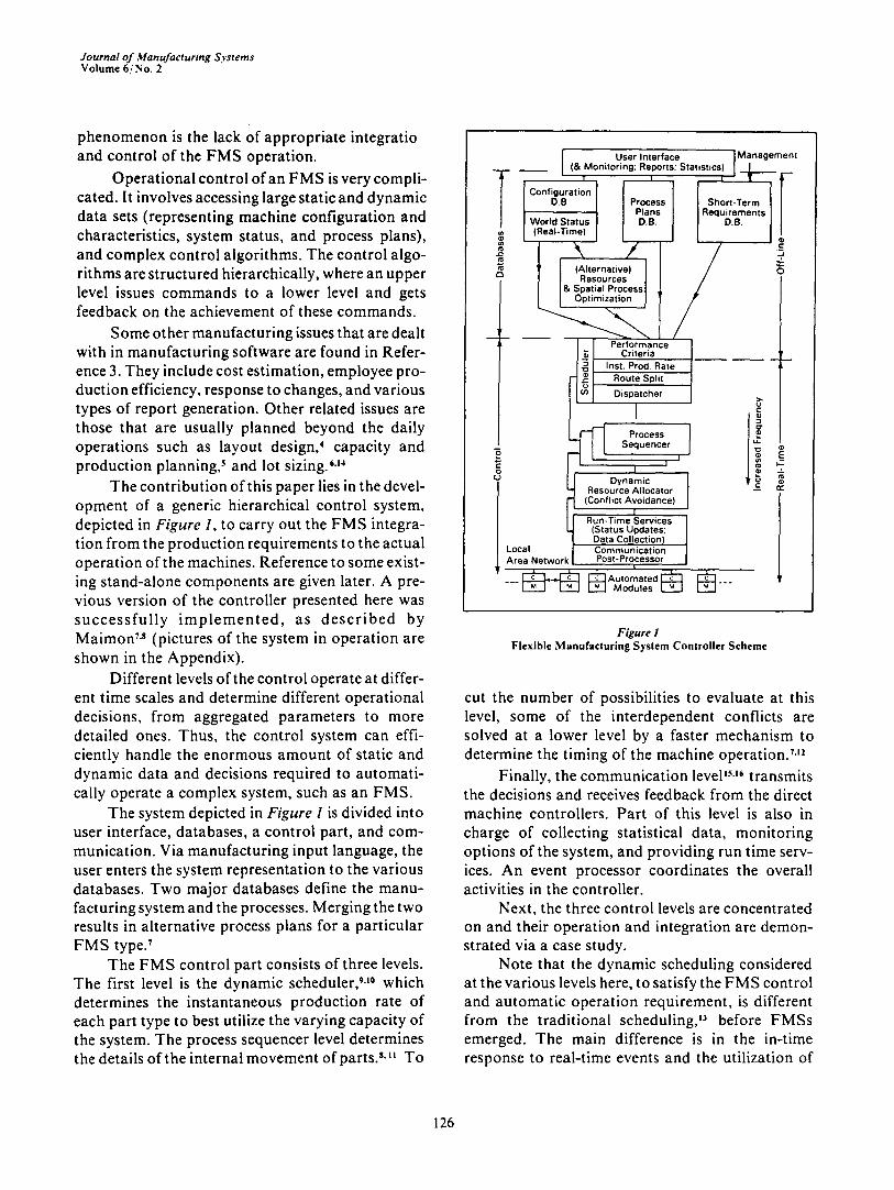
The organization of this level is depicted in Figure 2. The PS consists of three major components. The first is the knowledge base component where the facts and the rule set reside. In this component, knowledge about the process is represented in the form of process plans together with the required resources to achieve each step of the plan. For example, appropriate tools, jigs, and fixtures are specified. The setup times for the latter are represented as facts. The availability of appropriate resources are conditions to a particular operation and thus are represented as rules.

Plan from Upper Level

Global Databases • . . . . . . . . . . . . . . . . . . . . . . . . . . I Manufacturing System I Parameters I

I Algorithms

. . . . . . . . . . . . . . . . . ~ l n i e r e n c e I Process Plans & Resources

pSrY°SdeTt Sta ~s t e t" Er~gir~' { i~ii i i i i~ii! i i i i i i i i i i~ii '" II I I I Current Data

4, ........... I ........ *)

Update from the Factory Floor

I Feasible Set I I Possible Actions I I I

iiiiiiiiiii!iiiiiiiiiiiii I Action I I for Each Machine I I

Commands to Lower Level

Figure 2 Process Sequencer Organization

128


At this level, the particular manufacturing rules that apply to each specific FMS are represented. Those rules result from each system's possibilities and from the desired manufacturing practice in each FMS, as defined by the manufacturing or production engineer. For example, in the case of a certain queue length of parts in front of a machine, a robotic operation may be invoked to send some of the parts to another cell."

The second major component is where the system status and product ion state are held. This is where the constantly changing data of a manufacturing environment is kept. This data is required in order to make correct real-time decisions. The data includes information about machines being up or down or resource availability (such as which fixture is in use, or information about a broken tool).

The other set of data included here is the state of each part that is in production, how many operations were successfully completed so far, and the current location of the part. This local database relates to the main databases of the system where long-term information is maintained.

The third main component is the inference engine (IE). The IE presents the current system status and product ion state to the facts and the rules in order to come up with the feasible set. The feasible set is the collection of actions whose conditions have been fulfilled. For example, a part can continue on to several operations, but only one operation can actually take place. The latter deduction is also done by the IE using another level of abstrac-

tion of meta-rules (rules about rules), and algorithms. Then, based on the results of the action, the IE updates the system status and the production state. Thus, a cycle is completed and the next action should be determined.

The IE consists of four components: 1. IEflow control controls the flow of the pro-

gram, accepts interrupts (e.g., data f rom sensors that update the current status), and interacts with the rest of the software control (i.e., the event sequencer).

2. The local database manager updates and en- forces consistency when new data arrives. Two databases exist-- the status one and the internal working database which the IE develops when parsing the rules at various levels. This requires storing intermediate results.

3. The internalscheduler controls the order of the rules, takes care of hierarchical processing of the rules, and knows when to apply the various algorithms and heuristics.

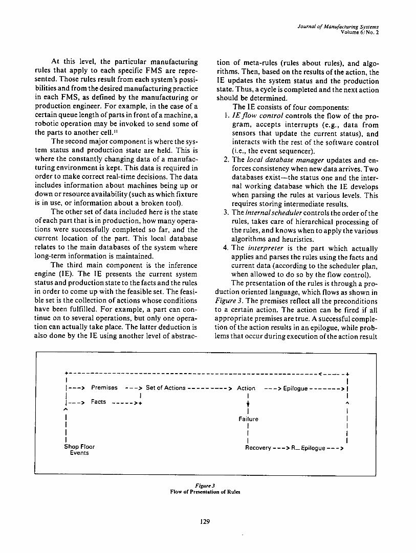
4. The interpreter is the part which actually applies and parses the rules using the facts and current data (according to the scheduler plan, when allowed to do so by the flow control). The presentation of the rules is through a pro-

duction oriented language, which flows as shown in Figure 3. The premises reflect all the preconditions to a certain action. The action can be fired if all appropriate premises are true. A successful completion of the action results in an epilogue, while problems that occur during execution of the action result

I [ - - - - ,

I [ - - - >

,A

I I I I Shop Floor

Events

P r e m i s e s - - - > Set o f A c t i o n s

I Facts . . . . . > +

• . . . . . 4-

I Action - - - • Epilogue . . . . . . . > I

I I

I I Fa i l u re I

I I I I I I

R e c o v e r y - - - > R _ Ep i l ogue - - - •

Figure 3 Flow of Presentation of Rules

129


in recovery actions and R-epilogue. The epilogues are used to update the premises and thus the cycle continues.

This f ramework of representation is particularly suited for the process sequencer level for two main reasons: it captures a manufactur ing process plan with all its particular conditions and mishaps that may occur; and it naturally lends itself to two modes of inference s t ra teg ies - -da ta -d r iven for normal operations and goal-driven when failure O c c u r s .

The data-driven method is used to derive the next action, after an epilogue has occurred. In principal, it is enough to use the modus ponens inference rule (recursively).

In general, the rules are expressed in the form of:

A Pi,ti -- (Aa~,xi) A (APi , t i ) for e a c h j e J

where/,, is a set of premises, which, if true, results in a set of actions, A, k e K i and a set of other premises Pt l e L i. There are a total of I JI such rules.

AnExample . I fx is feasible A cost (x) is low A priority (x) is high then select x, and y is feasible. And, if y is feasible A tool z is the system then select y.

PI A P2 A P 3 ~ A I A P4 P4 A P 5 - - A2

Now, resolution between A 1 and A2 is required to determine the next action. If only one action can be carried out, then either x or), should be selected.

Algorithms or heuristics are used for conflict resolution which results in an action. If failure occurs (i.e., unsuccessful action), rather than an "epilogue," recovery procedure has to take place. Recovery is referred to as actions taken to correct the fault operation that has happened, by restoring the device's (robot, machine) state to a state from which the process plan can be continued. This is the R-epilogue state. An example of recovery action is to return to the preconditions that led to the last action, e.g., restore the situation before the action has started.

Dynamic Resource Allocation Level. This level receives action requests (e.g., from several parts that share resources) and needs to arbitrate the actions when the required resources can simultaneously support only some of the actions so that no conflicts occur. The output of this level are corn-

mands to the communica t ion interface module to execute particular movements.

The objective of this level is to dynamically allocate the shared resources according to the next tasks to be performed in the FMS, complying with some priority policy (e.g., first in first out). This level is capable of synchronizing any number of requests to use shared resources while avoiding all potential conflict situations. An example is having the same tool or space required by more than one robot, or the same robot required to service several parts, at the same time.

The methodology here is by assigning a resource supervisor (RS) to each class of shared resources. The tasks of a resource supervisor are as follows:

1. Prevent access if the resource is occupied. 2. Queue requests for the occupied resource. 3. Allow conditional waiting for a particular sub-

class of resources. 4. Permit use of the resource to one of the queued

requests according to a policy and process plan.

5. Control the location and amount of each sub- class of the resource (e.g., different part types in a shared buffer).

6. Check the eligibility of requests for resource u s e .

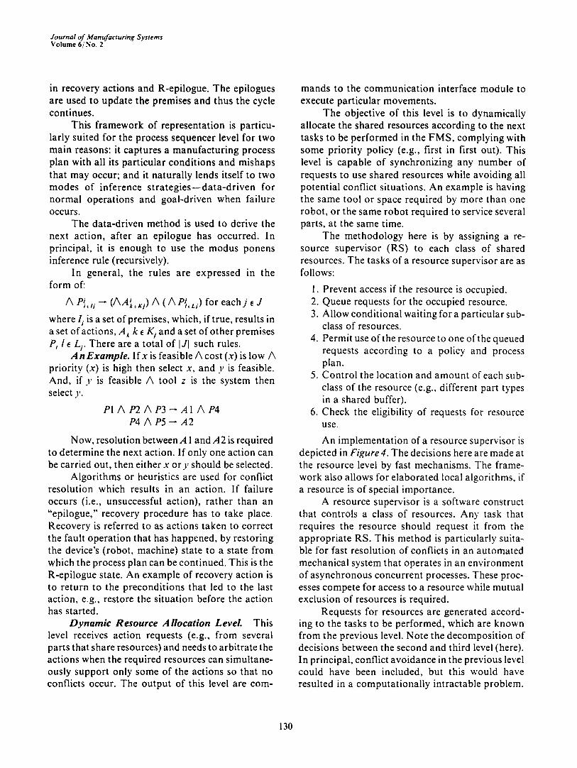
An implementation of a resource supervisor is depicted in Figure 4. The decisions here are made at the resource level by fast mechanisms. The framework also allows for elaborated local algorithms, if a resource is of special importance.

A resource supervisor is a software construct that controls a class of resources. Any task that requires the resource should request it from the appropriate RS. This method is particularly suitable for fast resolution of conflicts in an automated mechanical system that operates in an environment of asynchronous concurrent processes. These processes compete for access to a resource while mutual exclusion of resources is required.

Requests for resources are generated according to the tasks to be performed, which are known from the previous level. Note the decomposit ion of decisions between the second and third level (here). In principal, conflict avoidance in the previous level could have been included, but this would have resulted in a computat ional ly intractable problem.

130

Journal of Manufacturing Systems V o l u m e 6 / N o . 2

Requests

I Entrance = __ Entrance I Queue Filter I

Heading:

Local Variables Initialization

Procedure Get

Conditional Variables Check:

_ ~ Status Update: Conditional RS Exit

Queues

Procedure Put (Priorities.

Fn's) Conditional Variables Check:

- I Status Update:

Figure 4 Genera l Structure of a R e s o u r c e Supervisor

The size of the rule and the search spaces at the second level increase multiplicatively rather than linearly with the number of resources, by this decomposition.

Thus, in the previous level some intradepend- ent temporal rules do not have to be considered. At the second level, for example, two robots were assigned to pick two parts, one each. The temporal dependence (e.g., that a collision may happen if one robot starts its task within 8 t of the starting time of the other one) is resolved at the third level.

A request for a resource results in either grant- ing the resource or waiting in an ordered queue for the resource. When all resources required for a particular task are granted, the task is executed, and upon completion the resources are released. The resource supervisor then grants the resource to the first waiting request. Recall that the queue order can dynamically change.

The general structure of an RS for a resource RE is as follows:

Entrance Filter RS.RE

Variables declaration begin

Initialization (local variables) Procedure to obtain a resource:

Test status of resource if busy--->

Send request to a conditional queue

otherwise--> Grant the resource and Update resource status

Release the RS. Procedure to release a resource:

Test (depends on RE type) and Update resources status Release the RS.

end End RS.RE

An RS procedure is called by wait (S), where S is a semaphore RS.name.procedure name [actual parameters]. The code implementation of an RS varies depend- ing on the particular language and machine used.

Case Study In this section, the operation of concepts at the

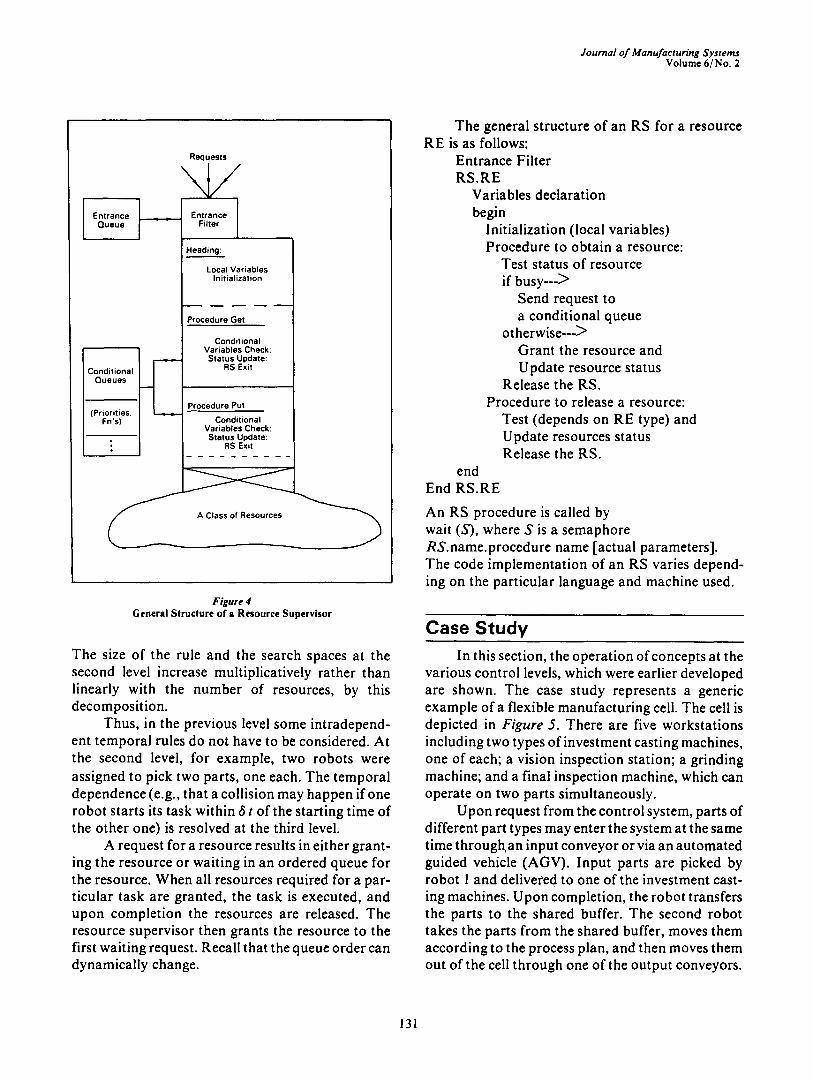
various control levels, which were earlier developed are shown. The case study represents a generic example of a flexible manufacturing cell. The cell is depicted in Figure 5. There are five workstations including two types of investment casting machines, one of each; a vision inspection station; a grinding machine; and a final inspection machine, which can operate on two parts simultaneously.

Upon request from the control system, parts of different part types may enter the system at the same time throughan input conveyor or via an automated guided vehicle (AGV). Input parts are picked by robot l and delivered to one of the investment casting machines. Upon completion, the robot transfers the parts to the shared buffer. The second robot takes the parts from the shared buffer, moves them according to the process plan, and then moves them out of the cell through one of the output conveyors.

131


Investment Casting

i , Robot 1

A~3t • I

AGV 2

z~put ; . . . . . . ; I i Conveyor I 1 I

~ / i o n System

. . . . . . . .

b u

e

r

I Grinding 4 l

Robot 2

1 2 1 1 I oot~ut t ~ I I I C°nvey °r

Figure 5 Flexible Manufacturing Cell

The controller of the two robots and the controller of the other direct machine are connected to a host, where the FMS controller resides. The FMS controller receives a signal upon a part entering or leaving the system. It can invoke specific tasks for each machine, including downloading appropriate programs to the various workstations, thus enabling them to operate on a variety of part types.

Consider simultaneous production of three different part types. Part type 1 requires investment casting of machine type I, and then is inspected by the vision system and the final inspection machine (the grinding is done in another cell); part type 2 uses the second investment casting machine and then moves to grinding and inspection; and part type 3 requires all but the second investment casting machine.

The scheduler which decides on the flow rates is first implemented and determines which part to load next to the system. This may require a request from an intercell-material handling control unit. The process sequencer then determines the next actions in the cell. The actions which may cause conflicts (e.g., collision between the two robots accessing the shared buffer) are filtered by the dynamic resource allocator. Finally, the communication module passes the commands to the machines to perform the actions.

The Scheduler Level. The model previously defined is used to determine the input flow of parts to the system to meet production demand, while considering the changing capacity constraints. The following are the system's input parameters:

1. Operation Time (Tii) for Each Part Type and Machine Characteristic

Machine \ Part Characteristics

Machine \ Type 1 I1 111 MTBF MTTR

! 28 0 40 20,000 2,000 2 0 43 0 20,000 2,000 3 40 0 10 40,000 3,000 4 0 30 30 25,000 2,000 5 20 30 30 15,000 4,000

Note: The data are given in time units (e.g.. seconds)

2. Penalty Function

x f o r x > = 0 g(x) = -10x f o r x < 0

The penalty function is the same for all part types. This means that all part types have the same relative importance. Backlog is penalized higher than positive surplus.

3. Demand Rate" and Machine Utilization (two cases are shown)

Demand 1 (do) Demand 2 (dL)

Part Type I 11 111 1 I1 111

Demand 0.017 0 .02 0.01 0.015 0.015 0.01

Machine Utilization .96 .95 .84 .97 .79 .90 .71 .75 .81 .66 (1 to 5)

* The demand rate is in parts/unit of time (seconds). The machine utilization is the fraction of the time required to meet demand to the total up-time of the machine.

4. Solution to the Scheduler Mode The first step of the solution is approximating

the value function, J, by a quadratic structure. To define the latter, and for the real-time level, only the A and b set of parameters are required. The value function parameters can be found by various methods. For brevity, the state-independent values are presented here, found by using a simple heuris- tic, based on the manufacturing meaning of these parameters.

Part Type: ! II 111 J parameters: A: 0.44 0.45 0.52

H: 22.50 20.00 13.75

132


The A value reflects vulnerability among part types. The more vulnerable the part is, the higher is its A value.

A " Y { M T T R / M T B F : mach ine visited}

H compensates for the average time lost by a machine being down, where:

- b d H - - M T T R m

A 2

M T T R - L

E { M T T R , : l e L }

where: L is the set of machines visited by a part type.

The hedging value H reflects building safety stock, when capacity is available, to account for possible future failure of machines.

Using those values, a simulation of the system was used to evaluate the product ion performance:

The simulat ion run for T equals 5 x l05 seconds. The product ion performance was mea- sured by three features:

I. P, = Product ion percentage = U i ( T ) / D i ( T ) 2. Balance = max P i /min P,. 3. C, = Cost per unit of time

C, = f~ g(x i ( t ) )d t evaluated numerically.

The product ion performance criteria measure how close to target the scheduler kept the production, the relative product ion levels of the various part types, and the model total cost value. In this example, notice from the product ion performance results that because of part type vulnerability, the system could not keep up with the higher demand (dH), though it was quite close to the d L demand.

5. Produc t ion Per formance Resul t s

Pa~ Type 1 I1 III I 11 II1

Ci 6290 9090 8040 2590 2360 3450 Pi 0.862 0.816 0.691 0.955 0.931 0.903

Balance 0.803 0.945

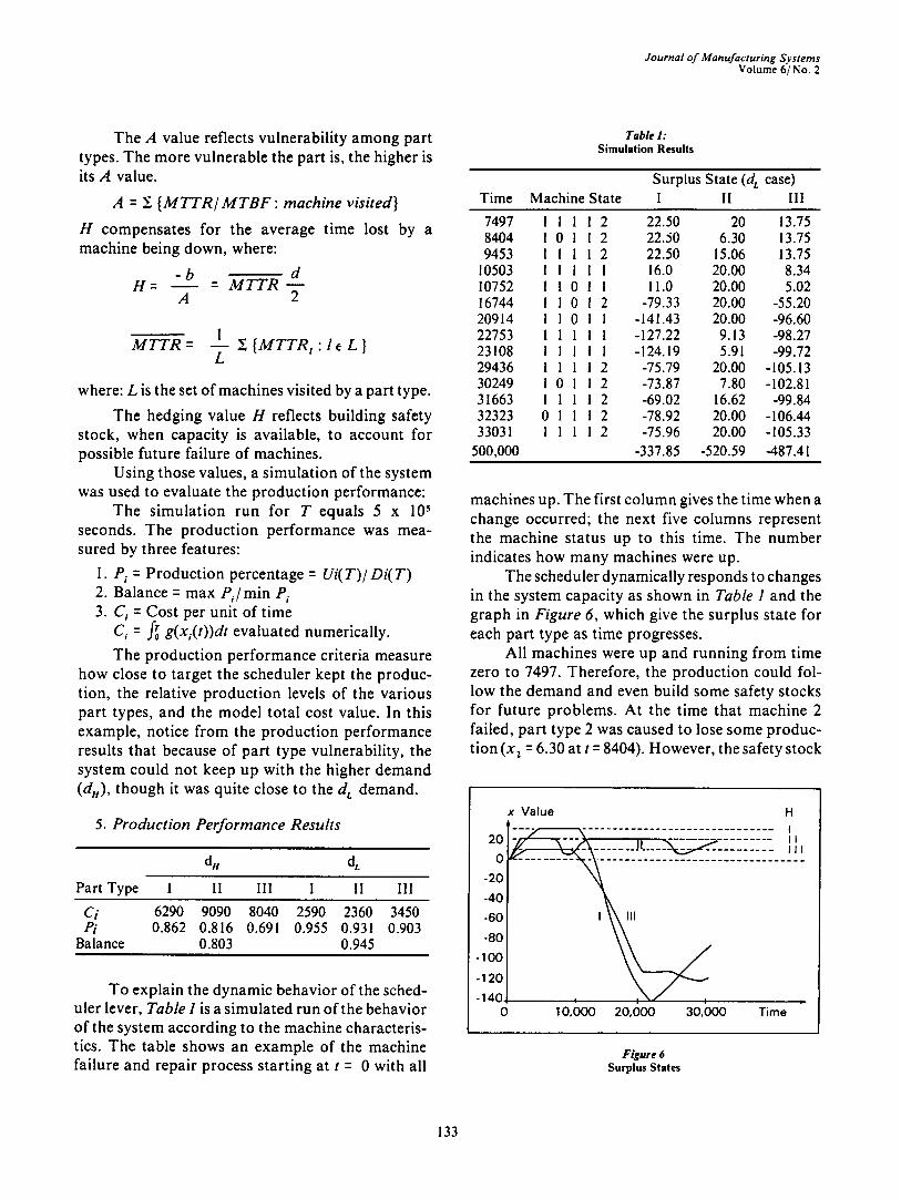
To explain the dynamic behavior of the scheduler lever, Table 1 is a simulated run of the behavior of the system according to the machine characteristics. The table shows an example of the machine failure and repair process starting at t = 0 with all

Table 1: Simulation Results

Surplus State (d t case) Time Machine State I II Ill

7497 8404 9453

10503 10752 16744 20914 22753 23108 29436 30249 31663 32323 33031

500,000

1 0 1 1 1 1 1 1 1 1 0 I

O l 1 1

1 2 1 2 1 2 1 1 0 i 0 2 0 1 1 l 1 1 1 2 1 2 1 2 1 2 1 2

22.50 20 13.75 22.50 6.30 13.75 22.50 15.06 13.75 16.0 20.00 8.34 I 1.0 20.00 5.02

-79.33 20.00 -55.20 - i 41.43 20.00 -96.60 -127.22 9.13 -98.27 -124.19 5.91 -99.72

-75.79 20.00 -105.13 -73.87 7.80 -102.81 -69.02 16.62 -99.84 -78.92 20.00 -106.44 -75.96 20.00 -105.33

-337.85 -520.59 -487.41

machines up. The first column gives the time when a change occurred; the next five columns represent the machine status up to this time. The number indicates how many machines were up.

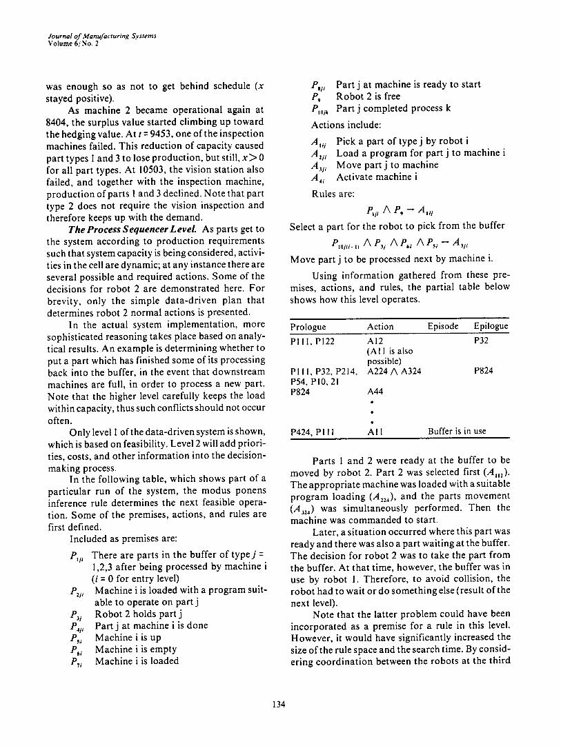
The scheduler dynamically responds to changes in the system capacity as shown in Table I and the graph in Figure 6, which give the surplus state for each part type as time progresses.

All machines were up and running from time zero to 7497. Therefore, the production could follow the demand and even build some safety stocks for future problems. At the time that machine 2 failed, part type 2 was caused to lose some production (x 2 = 6.30 at t = 8404). However, the safety stock

20

0

-20

-40

-60

-80

-100

-120

-140 0

x Value H

10.000 20,000 30,000 Time

Figure 6 Surplus States

133


was enough so as not to get behind schedule (x stayed positive).

As machine 2 became operat ional again at 8404, the surplus value started climbing up toward the hedging value. At t - 9453, one of the inspection machines failed. This reduct ion of capacity caused part types 1 and 3 to lose product ion , but still, x > 0 for all part types. At 10503, the vision station also failed, and together with the inspection machine, p roduc t ion of parts 1 and 3 declined. Note that part type 2 does not require the vision inspection and therefore keeps up with the demand.

TheProcess Sequencer Level. As parts get to the system according to product ion requirements such that system capacity is being considered, activities in the cell are dynamic; at any instance there are several possible and required actions. Some of the decisions for robot 2 are demonst ra ted here. For brevity, only the s imple da ta -dr iven plan that determines robot 2 normal actions is presented.

In the actual system implementat ion, more sophisticated reasoning takes place based on analy- tical results. An example is determining whether to put a part which has finished some of its processing back into the buffer, in the event that downst ream machines are full, in order to process a new part. Note that the higher level carefully keeps the load within capacity, thus such conflicts should not occur often.

Only level I of the data-driven system is shown, which is based on feasibility. Level 2 will add priorities, costs, and other informat ion into the decision- making process.

In the following table, which shows part of a part icular run of the system, the modus ponens inference rule determines the next feasible operation. Some of the premises, actions, and rules are first defined.

Included as premises are:

P~i~ There are parts in the buffer of t y p e j -- 1,2,3 after being processed by machine i (i -- 0 for entry level)

P~il Machine i is loaded with a program suitable to operate on part j

P~i Robot 2 holds part j P4ii Part j at machine i is done Ps~ Machine i is up P~; Machine i is empty PTi Machine i is loaded

Psii Part j at machine is ready to start /'9 Robo t 2 is free P~oik Part j completed process k

Actions include:

A, i Pick a part o f t y p e j by robot i A2i i Load a program for part j to machine i A3i i Move part j to machine A4. Activate machine i

Rules are:

Pl~ A P9 - - A ,~

Select a part for the robot to pick f rom the buffer

Ploi.. i~ A P3i A P61 A Psi -- A 3il

Move part j to be processed next by machine i.

Using informat ion gathered f rom these premises, actions, and rules, the partial table below shows how this level operates.

Prologue Action Episode Epilogue

P111, P122 Ai2 P32 (All is also possible)

P I l l , P32, P214, A224/~A324 P824 P54, PI0, 21 P824 A44

P424, Pi ! 1 AI 1 Buffer is in use

Parts 1 and 2 were ready at the buffer to be moved by robot 2. Part 2 was selected first (Am). The appropr ia te machine was loaded with a suitable p rogram loading (A~.), and the parts movement (A~.) was s imultaneously performed. Then the machine was c o m m a n d e d to start.

Later, a s i tuat ion occurred where this part was ready and there was also a part wait ing at the buffer. The decision for robot 2 was to take the part f rom the buffer. At that t ime, however, the buffer was in use by robot 1. Therefore, to avoid collision, the robo t had to wait or do someth ing else (result of the next level).

Note that the latter p roblem could have been incorporated as a premise for a rule in this level. However , it would have significantly increased the size of the rule space and the search time. By considering coord ina t ion between the robots at the third

134


level, this problem is avoided but with some cost (that of waiting or the need to switch tasks).

On the other hand, some of the rules regarding the machine status can be implemented in level 3, by an RS assigned to that machine. This will typically be the case in a larger FMS. Then, the action determined here is a request to the appropriate RS which resides in the third level.

Also, for brevity, the process plans of each part are not shown. They appear as premises with the alternatives and resources for each step, at this level.

The Dynamic Resource Allocation Level. At this level, consider the robots that share the same working envelope and buffer. If each robot action does not consider the other robot action, collision may occur. Also, the buffer has to be managed, i.e., where to put/ take each individual part. To solve these types of problems, two resource supervisors are in charge of the shared volume and the buffer, respectively. The program for robot 2 flows as follows:

<Robot 2 required to perform an action that needs the buffer>

j - RS.SB. Remove RS.SP.Get

<Robot 2 moves in and retrieves the part> RS.SP.Release

The robot first requests to remove the part, and finds out that the part is in location j; then it obtains permission to get into the shared space. Upon approval, it performs the operation, then releases the space. The RS.SP is a simple RS and can also be implemented by a binary semaphore. However, the structure of RS.SP is flexible to incorporate other requirements. If the space was occupied, the robot would be notified upon the freeing of the space, so that it could continue with its operation.

If the appropriate part is not in the buffer, the robot waits or performs another operation, while conditionally waiting for the part. Upon the arrival of the appropriate part, the robot is notified. The buffer management is locally done by the RS.SB resource supervisor. This RS is much more elabo- rate, as it controls and locally manages the buffer (e.g., where to put and from where to retrieve each part). The robot 1 program control flow is similar, using different features of the RS.SB.:

<Upon request to put a part in the buffer> RS.SB. Append (j) RS.SP. Get

< P u t part in shared buffer> RS.SP. Release

Concluding Remarks Some of the central notions of intelligent prob-

lem solving for large complex systems are appropriate modeling, aggregation, and the efficient solution of each level of aggregation with a much reduced space of alternatives.

The hierarchical control scheme for FMS operational control, suggested here, tries to do just that. The system is decomposed according to a time scale, different details of actions, and capacity utilization at each level. All levels operate in their real- time domain, responding to events that occur, utilizing the flexibility of the system at the various levels. Thus, the system controller can better meet the fast response time requirements (50 to 200 milliseconds at the high end).

The main contribution of this paper lies in the functional organization and decomposition of the problems that have to be solved by such a controller. Solutions are also suggested for each level. These solutions are appropriate when an industrial appli- cation can be characterized according to the model assumption. While it is true in many cases, there are applications that are different. Still, the solution scheme and decomposition scope of the problems defined here are generally appropriate, although detailed algorithms for each level may b e different. These algorithms are issues for future research.

Therefore, developing such an architecture has merit by itself. Currently for every implementation, one defines a new architecture and problem scope. This causes a prolonged and very expensive development process. Whenever implementing such an approach, one should carefully model the system and find appropriate solutions for each level, within the framework provided here.

Appendix Tasks ~ that require cooperation are shown.

Two robots are coordinated to transfer a part directly (one passes it to the other), or through a shared buffer.

135

Journal of Manufacturing Systems Volume 6~ No. 2

References 1. C. Dupont-Gatelmand. "A Survey of Flexible Manufacturing Sys-

tems", Journal of Manufacturing Systems, Volume I, No. I, 1982, pp. 1-16.

2. C. Boyle. "The Benefits of Group Technology Software for Manu- facturing", Proceedings of the IMTS, Chicago, IL, 1986, pp. 10.42-10.50. 3. D. Borg. "Software for Discrete Parts Manufacturing", Proceed-

ings of the IMTS, Chicago, IL, 1986, pp. 10.2-10.19. 4. P. Afentakis, R.A. Millen, M.M. Solomon. "Layout Design for

Flexible Manufacturing System: Models and Strategies". Proceedings of the Second ORSA/ TIMS Conference on Flexible Manufacturing Systems, (K.E. Stecke, R. Suri, eds.), Elsevier Publications, 1986. pp. 221-231.

5. A. Hax, M. Meal. "'Hierarchical Integration of Production Plan- ning and Scheduling", TIMS Studies in Management Science, Volume I: Logistics, (M. Geisler, ed.), Elsevier Publications, t975. 6. Y.L. Chang, R.S. Sullivan. "Lot Sizing in a Flexible Assembly

System", Proceedings of the Second ORSA/TIMS Conference on Flexible Manufacturing Systems, (K.E. Stecke, R. Suri, eds.), Elsevier Publications, 1986, pp. 359-367. 7. O. Maimon. "A Generic Flexible Multirobot Experimental Sys-

tem". Journal of Robotic Systems, Volume 3, No. 4, 1986. 8. O. Maimon. "Intelligent Material Handling Control Systems", Dig-

ital Equipment Co., March 1986. 9. S.B. Gershwin, R. Akella, Y. Choong. "Short-Term Scheduling of

an Automated Manufacturing Facility", IBM Journal of Research and Development, Volume 29, No. 4, 1985, pp. 392-400. 10. O. Maimon, S.B. Gershwin. "'Dynamic Scheduling and Routing for FMS that have Unreliable Machines", MIT. LIDS-P 1610. 1986. !1. K.Y. ,Io, O. Maimon. "Optimal Dynamic Load Distribution in Flexible Manufacturing System", Technical Report No. 5, Center for Computational Probability and Statistics, George Mason University. 1986. 12. O. Maimon, G. Tadmor. "Efficient Low-Level Control of FMS", MIT, LIDS-P-1571, 1986. 13. C.S. Graves. "A Review of Production Scheduling", Operations Research, Volume 29, No. 4, 1981, pp. 646-675. 14. S.B. Gershwin. "Stochastic Scheduling and Set-Ups in Flexible Manufacturing Systems", Proceedings of the Second ORSA/TIMS Conference on Flexible Manufacturing Systems, (K .E. Stecke, R. Suri, eds.), Elsevier Publications, 1986, pp. 461-467. 15. Digital Equipment Corporation, Baseway and Shop Floor Gateway, SPD 14.85.02, January 1986. 16. General Motors Corporation, Manufacturing Automation Proto- col, MAP Specifications V.2.2, GM Tech Center, 1986.

Author Biography Oded Z. Maimon is on the faculty of Industrial Engineering at Tel Aviv University, Israel. Previously, he

held a joint appointment at DEC's Computer Integrated Manufacturing Group and at the Massachusetts Institute of Technology's Laboratory for Information and Decision Systems. He received a B.S.I.E., a B.S.M.E. and an M.S. in Operations Research from the Technion in Israel, and a Ph.D. from Purdue University, W. Lafayette, Indiana.

Dr. Maimon's research and development interests are in the planning, analysis, and automatic operational control of flexible manufacturing systems, in general, and in robotic systems, in particular. He has published in the Transactions of the ASME, the IEEE Journal of Robotics and Automation, Annals of Operations Research, the liE Transactions, the Journal of Robotic Systems, and others.

136

Documents

Real-time operational control of flexible manufacturing systems