Reconstructing Shape and Motion from Asynchronous Cameras … · F.Klose, C.Lipski, M.Magnor / Reconstructing Shape and Motion from Asynchronous Cameras views of a single object

Vision, Modeling, and Visualization (2010)Reinhard Koch, Andreas Kolb, Christof Rezk-Salama (Eds.)

Reconstructing Shape and Motionfrom Asynchronous Cameras

Felix Klose1, Christian Lipski1, Marcus Magnor1

1Computer Graphics Lab, TU Braunschweig

Abstract

We present an algorithm for scene flow reconstruction from multi-view data. The main contribution is its abilityto cope with asynchronously captured videos. Our holistic approach simultaneously estimates depth, orientationand 3D motion, as a result we obtain a quasi-dense surface patch representation of the dynamic scene. Thereconstruction starts with the generation of a sparse set of patches from the input views which are then iterativelyexpanded along the object surfaces. We show that the approach performs well for scenes ranging from singleobjects to cluttered real world scenarios.

This is the author version of the paper. The definitive version is available at digilib.eg.org.

Categories and Subject Descriptors (according to ACM CCS): I.4.8 [Image Processing and Computer Vision]: SceneAnalysis—Stereo, Time-varying imagery

1. Introduction

With the wide availability of consumer video cameras andtheir ever increasing quality at lower prices, multi-viewvideo acquisition has become a widely popular researchtopic. Together with the large amount of processing powerreadily available today, multiple views are used as input datafor high quality reconstructions. While the traditional two-view stereo reconstruction extends well to a multi-view sce-nario for static scenes, the complexity increases for sceneswith moving objects. The most common way of approachingthis problem is the use of synchronized image acquisition.

To loose the limitations that synchronized acquisition se-tups impose, we present our multi-view reconstruction ap-proach that takes asynchronous video as input. Hence, nocustom and potentially costly hardware with synchronizedshutters is needed.

Traditional reconstruction algorithms rely on synchronousimage acquisition, so that they can exploit the epipolar con-straint. We eliminate this limitation and furthermore bene-fit from the potentially higher temporal sampling due to thedifferent shutter times. With our approach, scene flow re-construction with rolling shutters as well as heterogeneous

temporal sampling, i.e. cameras with different framerates, ispossible.

In Sect. 2 we give a short overview of the current research.Sect. 3 then gives an overview our algorithm. A detailed de-scription of our approach is then given in Sect. 5-8, followedby our experimental results in Sect. 9, before we conclude inSect. 10.

2. Related Work

When evaluating static multi-view stereo (MVS) algorithms,Seitz et al. [SCD∗06] differentiated the algorithms by theirbasic assumptions. Grouping algorithms by their underlyingmodel provides four categories: The volumetric approachesusing discrete voxels in 3D space [KKBC07, SZB∗07], thealgorithms that evolute a surface [FP09b], reconstructionsbased on depth map merges [MAW∗07, BBH08] and algo-rithms are based on the recovery of 3D points that are thenused to build a scene model [FP09a, GSC∗07].

While all the MVS approaches recover a scene modelfrom multiple images, the limitations on the scene shown onthe images vary. Algorithms that are based on visual hullsor require a bounding volume are more suited for multiple

c© The Eurographics Association 2010.

digilib.eg.org

F.Klose, C.Lipski, M.Magnor / Reconstructing Shape and Motion from Asynchronous Cameras

views of a single object. The mentioned point based meth-ods on the other hand perform well on single objects andcluttered scenes.

Regarding the objective of scene motion recovery, theterm scene flow was coined by Vedula [VBR∗99]. The 3Dscene flow associates a motion vector with each input im-age point, corresponding to its velocity in scene space. Theexisting approaches to recover scene flow can be split intothree groups based in their input data. The first group uti-lizes multiple precomputed optical flow fields to computethe scene flow [ZK01, VBR∗05]. The second uses static 3Dreconstructions at discrete timesteps and recovers the mo-tion by registering the data [ZCS03,PKF05,PKF07]. A thirdfamily of algorithms uses spatio-temporal image derivativesas input data [NA02, CK02].

Besides the obvious connection between the structure andits motion, in current research the recovery largely remainssplit into two disjunct tasks. Wang et al. [WSY07] pro-posed an approach to cope with asynchronously captureddata. However, their two-step algorithm relies on synthesiz-ing synchronized intermediate images, which are then pro-cessed in a traditional way.

Our holistic approach simultaneously recovers geometryand motion without resampling the input images. We basethe pipeline of our approach on the patch-based MVS by Fu-rukawa et al. [FP09a], which showed impressive results forthe reconstruction of static scenes. While Furukawa et al. ex-plicitly remove non-static objects, i.e., spatially inconsistentscene parts, from scene reconstruction, we create a dynamicscene model where both object geometry and motion are re-covered. Although we adapt the basic pipeline design, ourrequirement to cope with dynamic scenes and to reconstructmotion make fundamental changes necessary. E.g., our ini-tialization and optimization algorithms have to take individ-ual motion of a patch into account.

3. Overview

We assume that the input video streams show multiple viewsof the same scene. Since we aim to reconstruct a geometricmodel, we expect the scene to consist of opaque objects withmostly diffuse reflective properties.

In a preprocessing step the in- and extrinsic camera pa-rameters for all images are estimated by sparse bundle ad-justment [SSS06]. Additionally the sub-frame time offsetsbetween the cameras have to be determined. Different meth-ods have been explored in recent research to automaticallyobtain the sub-frame offset [MSMP08, HRT∗09].

The algorithm starts by creating a sparse set of seed pointsin an initialization phase, and grows the seeds to cover thevisible surface by iterating expansion, optimization and filtersteps.

Our scene model represents the scene geometry as a set

of small tangent plane patches. The goal is to reconstructa tangent patch for the entire visible surface. Each patch isdescribed by its position, normal and velocity vector.

The presented algorithm processes an image group at atime, which consists of images chosen by their respectivetemporal and spatial parameters. All patches extracted froman image group collectively form a dynamic model of thescene, that is valid for the timespan of the image group. Theimage group timespan is the time interval ranging from theacquisition of the first image of the group to the time the lastselected image was recorded.

Since the scene model has a three dimensional velocityvector for each surface patch, linear motion in the scenespace is reconstructed. The motion only needs to be linearfor the image group timespan.

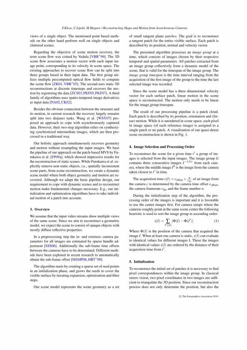
The result of our processing pipeline is a patch cloud.Each patch is described by its position, orientation and (lin-ear) motion. While it is unordered in scene space, each pixelin image space (of each reference image) is assigned to asingle patch or no patch. A visualization of our quasi-densescene reconstruction is shown in Fig. 1.

4. Image Selection and Processing Order

To reconstruct the scene for a given time t′ a group of im-ages is selected from the input images. The image group Gcontains three consecutive images I−1,0,1 from each cam-era, where the middle image I0 is the image from the camerataken closest to t′ in time.

The acquisition time t(I) = coffset +n

cfpsof an image from

the camera c is determined by the camera time offset coffset,the camera framerate cfps and the frame number n.

During the initialization step of the algorithm, the pro-cessing order of the images is important and it is favorableto use the center images first. For camera setups where thecameras roughly point at the same scene center the followingheuristic is used to sort the image group in ascending order:

s(I) = ∑I′∈G|Φ(I)−Φ(I′)| (1)

Where Φ(I) is the position of the camera that acquired theimage I. When at least one camera is static, s(I) can evaluateto identical values for different images I. These the imageswith identical values s(I) are ordered by the distance of theiracquisition time from t′.

5. Initialization

To reconstruct the initial set of patches it is necessary to findpixel correspondences within the image group. In classicalstereo vision, two pixel coordinates in two images are suffi-cient to triangulate the 3D position. Since our reconstructionprocess does not only determine the position, but also the



Figure 1: Visualization of reconstructed scenes. The patches are textured according to their reference image. Motion is visual-ized by red arrows.

velocity of a point in the scene, more correspondences areneeded.

The search for correspondences is further complicated bythe nature of our input data. One of the implications of theasynchronous cameras is, that no epipolar geometry con-straints can be used to reduce the search region for the pixelcorrespondence search.

We compute a list of interest points for each image I′ ∈G.An Harris Corner detector is used to select the points of in-terest. The intention is to select points which can be identi-fied across multiple images. A local maximum suppressionis performed, i.e., only the strongest response within a smallradius is considered. Every interest point is then describedby a SURF [BETG08] descriptor. In the following, an inter-est point and its descriptor is referred to as a feature.

For each image I′, every feature f extracted from thatimage is serially processed. A given feature f0 is matchedagainst all features from the other images. The best matchfor each image is added into a candidate set C.

The candidate set C may contain outliers. This is due towrong matchings and the fact, that the object on which f0 islocated may not be visible in all camera images. A subset forreconstructing the surface patch has to be selected. To findsuch a subset a RANSAC based method is used:

First a set S of Θ− 1 features is randomly sampled fromC. Then the currently processed feature f0 is added to the setS. The value of |S|= Θ can be varied depending on the inputdata. For all our experiments we chose Θ = 6.

The sampled features in S are assumed to be evidence ofa single surface. Using the constraints from feature positionsand camera parameters and assuming a linear motion model,a center position~c and a velocity~v are calculated. The detailsof the geometric reconstruction are given later (section 5.1).

The vectors~c and~v represent the first two parameters of anew patch P. The next RANSAC step is to determine whichfeatures from the original candidate set C consent to the re-constructed patch P. The patch is reprojected into the imagesI′ ∈ G and the distance from the projected position to thefeature position in I′ is evaluated. After multiple RANSAC

iterations the largest set T ⊂C of consenting features foundis selected.

Although the reconstruction equation system is alreadyoverdetermined by the |T | matched features, the data tendsto be degenerated and leads to unsatisfying results. The de-generation is caused by too small baselines along one ormultiple of the spatial axes of the camera positions, as wellas the temporal axis. As a result of the insufficient informa-tion in the input data, patches with erroneous position andvelocity are reconstructed.

Under the assumption that sufficient information ispresent in the candidate set C to find the correct patch, theinitialization algorithm enriches the set T , using a greedyapproach.

To find more information that is coherent with the currentreconstruction more features f ′ ∈ C \ T need to be addedto T . Each feature f ′ is accepted into T if the patch recon-structed from T ′ = T ∪ { f ′} has at least T ′ as consentingfeature set.

After the enrichment of T the final set of consenting fea-tures is used to calculate the position and velocity for thepatch P′. To fully initialize P′, two more parameters need tobe set. The first is the reference image of the patch, whichhas two different uses. If I is the reference image of P′ thanthe acquisition time tr = t(I) marks the point when the patchP′ is observed at the reconstructed center position ~c. As aresult the scene position pos(P′, t′) of P′ at any given timet′ is:

pos(P′, t′) =~c+(t′− tr) ·~v. (2)

Furthermore, the reference image is used in visibility calcu-lations, where a normalized cross correlation is used. Thecorrelation template for a patch P′ is extracted from its ref-erence image. The reference image for P′ is the image theoriginal feature f0 was taken from. The last parameter for P′

is the surface orientation represented by the patch normal.The normal of P′ is coarsely approximated by the vectorpointing from ~c to the center of the reference image cam-era. When the patch has been fully initialized, it is added tothe initial patch generation.



After all image features have been processed the initialpatch generation is optimized and filtered once before theexpand and filter iterations start.

5.1. Geometric Patch Reconstruction

Input for the geometric patch reconstruction is a list of corre-sponding pixel positions in multiple images combined withthe temporal and spatial position of the cameras. The resultis a patch center~c and velocity~v.

Assuming a linear movement of the scene point, its posi-tion~x(t) at the time t is specified by a line

~x(t) =~c+ t ·~v. (3)

To determine ~c and ~v, a linear equation system is formu-lated. The line of movement (3) must intersect the viewingrays ~qi that originate from the camera center Φ(Ii) and arecast through the image plane at the pixel position where thepatch was observed in image t i = t(Ii):

Id3×3 Id3×3 · t0 −~q T

0 0 0...

.... . .

Id3×3 Id3×3 · t i 0 0 −~q Ti

·

~cT

~vT

a0

...a j

=

Φ(I0)

T

...Φ(Ii)T

(4)

The variables a0 to a j give the scene depth in respect tothe camera center Φ(Ib

j3 c) and are not further needed. The

overdetermined linear system is solved with a SVD solver.

5.2. Patch Visibility Model

There are two sets of visibilities associated with every patchP. The set of images where P might be visible V (P) and theset of images where P is considered truly visible V t(P) ⊂V (P). The two different sets exist to deal with specular high-lights or not yet reconstructed occluders.

During the initialization process the visibilities are de-termined by thresholding a normalized cross correlation. Ifν(P, I) is the normalized cross correlation calculated fromthe reference image of P to the image I, then V (P) ={I|ν(P, I) > α} and V t(P) = {I|ν(P, I) > β}. The thresh-old parameters used in all our experiments are α = 0.45 andβ = 0.8. The correlation function ν takes the patch normalinto account when determining the correlation windows.

In order to have a efficient lookup structure for patcheslater on, we overlay a grid of cells over every image. In ev-ery grid cell all patches are listed, that when projected tothe image plane, fall into the given cell and are consideredpossibly or truly visible in the given image.

The size of the grid cells λ and the resulting resolutiondetermines the final resolution of our scene reconstruction

Ir

~cP

(a)

Ir

P

(b)

I′Ir

P (t′− tr) ·~v~c

(c)

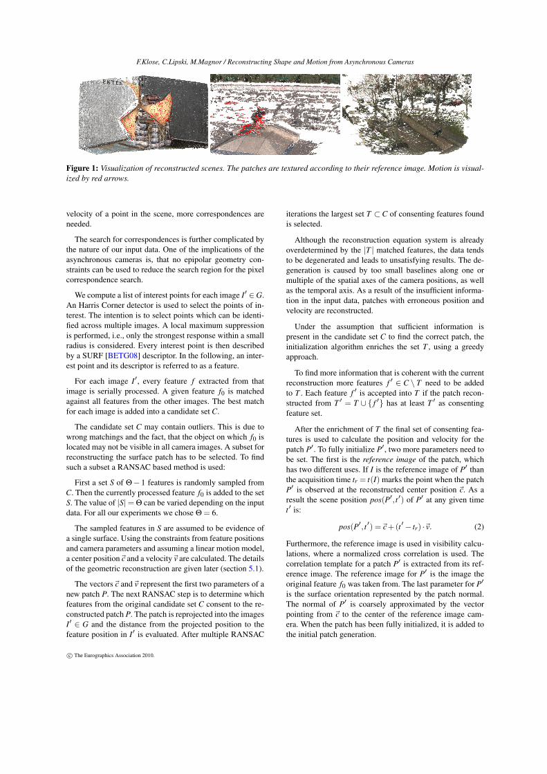
Figure 2: Computing cross correlation of moving patches.(a) A patch P is described by its position ~c, orientation,recording time tr and its reference image Ir. (b) Positionsof sampling points are obtained by casting rays through theimage plane (red) of Ir and intersecting with plane P. (c) Ac-cording to the difference in recording times (t′− tr) and themotion~v of the patch, the sampling points are translated, be-fore they are projected back to the image plane of I′. Crosscorrelation is computed using the obtained coordinates inimage space of I′.

as only one truly visible patch in each cell in every imageis calculated. We experienced that it is a valid strategy tostart with a higher λ (e.g. λ ≥ 2) for an initial quasi-densereconstruction, followed by a reconstruction at pixel level(λ = 1).

The grid structure is also used to perform the visibilitytests during the expand and filter iterations.

The visibility of P is estimated by a depth comparisonwithin the grid cells. All images, for which P is closer to thecamera than the currently closest patch in the cell, are addedto V (P). The images I′ ∈V t(P′), where the patch is consid-ered truly visible, are determined using the same method ofcomparing ν against β as before, except that the threshold islowered with increasing expansion iteration count to coverpoorly textured regions.

6. Expansion phase

The initial set of patches is usually very sparse. To incre-mentally cover the entire visible surface, the existing patchesare expanded along the object surfaces. The expansion algo-rithm processes each patch from the current generation.

In order to verify if a given patch P should be expanded,all images I ∈V t(P) where P is truly visible are considered.Given the patch P and a single image I, the patch is pro-jected into the image plane and the surrounding grid cellsare inspected. If a cell is found where no truly visible patchexists yet, a surface expansion of P to the cell is calculated.



A viewing ray is cast through the center of the empty celland intersected with the plane defined by the patches posi-tion at t(I) and its normal. The intersection point is the cen-ter position for the newly created patch P′. The velocity andnormal of the new patch are initialized with the values fromthe source patch P. At this stage, P′ is compared to all otherpatches listed in its grid cell and is discarded if another sim-ilar patch is found. To determine whether two patches aresimilar in a given image, their position ~x0,~x1 and normals~n0,~n1 are used to evaluate the inequality

(~x0~x1) ·~n0 +(~x1~x0) ·~n1 < κ. (5)

The comparison value κ is calculated from the pixel dis-placement of λ pixels in image I and corresponds to thedepth displacement which can arise within one grid cell. Ifthe inequality holds, the two patches are similar.

Patches that are not discarded are processed further. Thereference image of the new patch P′ is set to be the image Iin which the empty grid cell was found. The visibility of P′

is estimated by a depth comparison as described in 5.2. Be-cause the presence of outliers may result in a too conserva-tive estimation of V (P′), the visibility information from theoriginal patch is added V (P′) = V (P′)∪V (P) before calcu-lating V t(P′).

After the new patch is fully initialized, it is handed intothe optimization process. Finally, the new patch is acceptedinto the current patch generation, if |V t(P′)| ≥ φ. The leastnumber of images to accept a patch is dependent on the cam-era setup and image type. With increasing φ less surface canbe covered with patches on the outer cameras, since eachsurface has to be observed multiple times. Choosing φ toosmall may result in unreliable reconstruction results.

7. Patch Optimization

The patch parameters calculated from the initial reconstruc-tion or the expansion are the starting point for a conjugategradient based optimization. The function ρ maximized is avisibility score of the patch. To determine the visibility scorea normalized cross correlation ν(P, I) is calculated from thereference image of P to all images I ∈ V (P) where P is ex-pected to be visible:

ρ(P) =1

|V (P)|+ a · |V t(P)|

(∑

I∈V (P)

ν(P, I)+ ∑I∈V t (P)

a ·ν(P, I))

(6)

The weighting factor a accounts for the fact that imagesfrom V t(P) are considered reliable information, while im-ages from V (P) \V t(P) might not actually show the scenepoint corresponding to P. The visibility function ρ(P) is thenmaximized with a conjugate gradient method.

To constrain the optimization, the position of P is notchanged in three dimensions, but in a single dimension rep-resenting the depth of P in the reference image. The variation

of the normal is specified by two rotation angles and at lastthe velocity is left as three dimensional vector. The resultingproblem has six dimensions.

8. Filtering

After the expansion step the set of surface patches possiblycontains visual inconsistencies. These inconsistencies can beput in three groups. The outliers outside the surface, outliersthat lie inside the actual surface and patches that do not sat-isfy a regularization criterion. Three distinct filters are usedto eliminate the different types of inconsistencies.

The first filter deals with outliers outside the surface. Todetect an outlier a support value s and a doubt value d iscomputed for each patch P. The support is the patch scoreEq. (6) multiplied by the number of images where P is trulyvisible s = ρ(P) · |V t(P)|. Summing the score of all patchesP′ that are occluded by P gives a measure for visual incon-sistency introduced by P and is the doubt d. If the doubt out-weighs the support d > s the patch is considered an outlierand removed.

Patches lying inside the surface will be occluded by thepatch representing the real surface, therefore the visibilitiesof all patches are recalculated as described in 5.2. After-wards, all patches that are not visible in at least φ imagesare discarded as outliers.

The regularization is done with the help of the patch sim-ilarity defined in Eq. (5). In the images where a patch P isvisible all surrounding c patches are evaluated. The quotientof the number c′ of patches similar to P in relation to the totalsurrounding patches c is the regularization criterion: c′

c < z.The quotient of the similarly aligned patches was z = 0.25in all our experiments.

9. Results

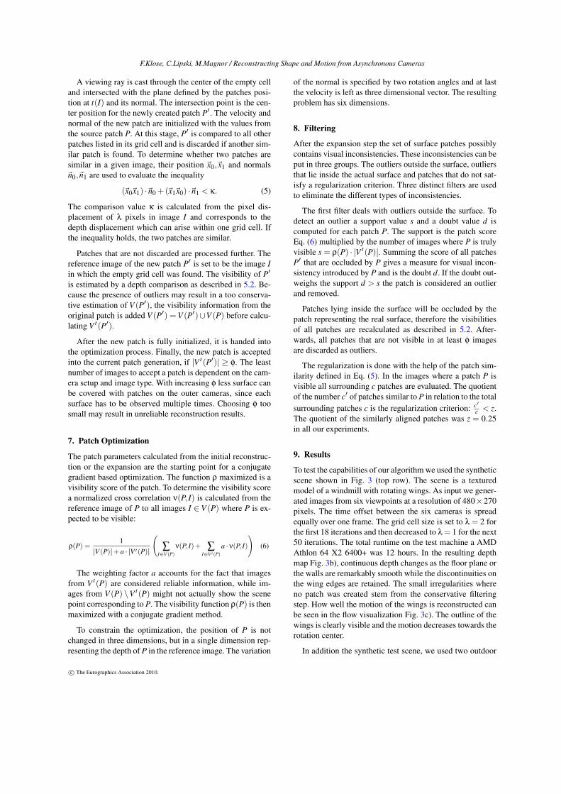
To test the capabilities of our algorithm we used the syntheticscene shown in Fig. 3 (top row). The scene is a texturedmodel of a windmill with rotating wings. As input we gener-ated images from six viewpoints at a resolution of 480×270pixels. The time offset between the six cameras is spreadequally over one frame. The grid cell size is set to λ = 2 forthe first 18 iterations and then decreased to λ = 1 for the next50 iterations. The total runtime on the test machine a AMDAthlon 64 X2 6400+ was 12 hours. In the resulting depthmap Fig. 3b), continuous depth changes as the floor plane orthe walls are remarkably smooth while the discontinuities onthe wing edges are retained. The small irregularities whereno patch was created stem from the conservative filteringstep. How well the motion of the wings is reconstructed canbe seen in the flow visualization Fig. 3c). The outline of thewings is clearly visible and the motion decreases towards therotation center.

In addition the synthetic test scene, we used two outdoor



(a) (b) (c)

Figure 3: (a) Input views, (b) quasi-dense depth recon-struction and (c) optical flow to the next frame. For thesynthetic windmill scene, high-quality results are obtained.When applied to the more challenging real-world scenes(skateboarder scene, middle, parkours scene, bottom), ro-bust and accurate results are still obtained. The conservativefiltering prevents the expansion to ambiguous regions. E.g.,most pixels in the asphalt region in the skateboarder sceneare not recovered. All moving regions except the untexturedbody of the parkours runner were densely reconstructed,while some motion outliers remain in the background.

sequences. The resolution for both scenes was 960× 540pixels. The skateboarder scene, Fig. 3 (middle row), wasfilmed with six unsynchronized cameras and chosen becauseit has a large depth range and fast motion. The skateboarderand the ramp in the foreground as well as the trees in thebackground are reconstructed in great detail, Fig. 3b). Theasphalt area offers very little texture. Due to our restrictivefiltering, it is not fully covered with patches. The motion ofthe skater and that of his shadow moving on the ramp is vis-ible in 3c). The shown results were obtained after 58 itera-tions starting with λ = 2 and using λ = 1 from iteration 55onward. The total computation time was 95 hours.

The second real world scene Fig. 3 (bottom row) featuresa setup of 16 cameras showing a parkours runner jumpinginto a handstand. The scene has a highly cluttered back-ground geometry. Similar to the skateboard scene, regionswith low texture are not covered with patches. However, de-tails of the scene are clearly visible in the depth map and themotion reconstructed for the legs and the back of the personis estimated very well. Due to the cluttered geometry and thelarge number of expansion steps, the reconstruction took 160

(a) (b) (c)

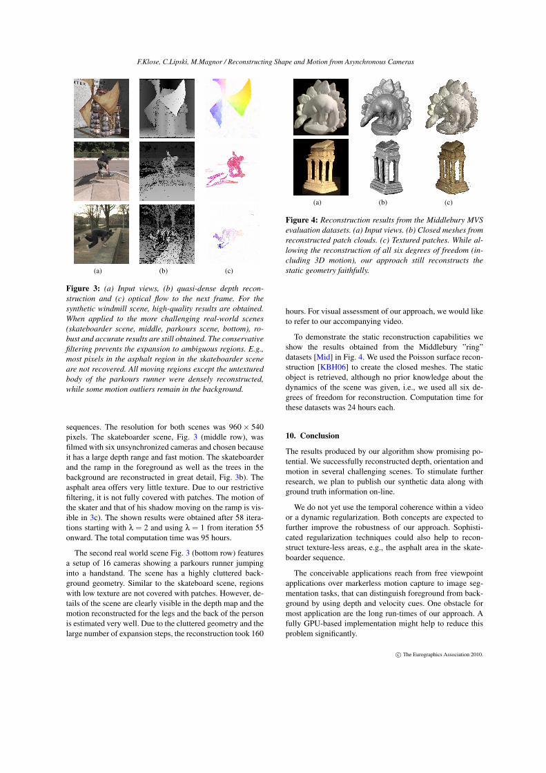
Figure 4: Reconstruction results from the Middlebury MVSevaluation datasets. (a) Input views. (b) Closed meshes fromreconstructed patch clouds. (c) Textured patches. While al-lowing the reconstruction of all six degrees of freedom (in-cluding 3D motion), our approach still reconstructs thestatic geometry faithfully.

hours. For visual assessment of our approach, we would liketo refer to our accompanying video.

To demonstrate the static reconstruction capabilities weshow the results obtained from the Middlebury ”ring”datasets [Mid] in Fig. 4. We used the Poisson surface recon-struction [KBH06] to create the closed meshes. The staticobject is retrieved, although no prior knowledge about thedynamics of the scene was given, i.e., we used all six de-grees of freedom for reconstruction. Computation time forthese datasets was 24 hours each.

10. Conclusion

The results produced by our algorithm show promising po-tential. We successfully reconstructed depth, orientation andmotion in several challenging scenes. To stimulate furtherresearch, we plan to publish our synthetic data along withground truth information on-line.

We do not yet use the temporal coherence within a videoor a dynamic regularization. Both concepts are expected tofurther improve the robustness of our approach. Sophisti-cated regularization techniques could also help to recon-struct texture-less areas, e.g., the asphalt area in the skate-boarder sequence.

The conceivable applications reach from free viewpointapplications over markerless motion capture to image seg-mentation tasks, that can distinguish foreground from back-ground by using depth and velocity cues. One obstacle formost application are the long run-times of our approach. Afully GPU-based implementation might help to reduce thisproblem significantly.



References

[BBH08] BRADLEY D., BOUBEKEUR T., HEIDRICH W.: Accu-rate multi-view reconstruction using robust binocular stereo andsurface meshing. In IEEE Conference on Computer Vision andPattern Recognition, 2008. CVPR 2008 (2008), pp. 1–8. 1

[BETG08] BAY H., ESS A., TUYTELAARS T., GOOL L. V.:Surf: Speeded up robust features. Computer Vision and ImageUnderstanding 110, 3 (2008), 346–359. 3

[CK02] CARCERONI R., KUTULAKOS K.: Multi-view scenecapture by surfel sampling: From video streams to non-rigid 3Dmotion, shape and reflectance. International Journal of Com-puter Vision 49, 2 (2002), 175–214. 2

[FP09a] FURUKAWA Y., PONCE J.: Accurate, dense, and robustmulti-view stereopsis. IEEE Trans. on Pattern Analysis and Ma-chine Intelligence (2009). 1, 2

[FP09b] FURUKAWA Y., PONCE J.: Carved visual hulls forimage-based modeling. International Journal of Computer Vi-sion 81, 1 (2009), 53–67. 1

[GSC∗07] GOESELE M., SNAVELY N., CURLESS B., HOPPEH., SEITZ S.: Multi-view stereo for community photo collec-tions. In IEEE International Conference on Computer Vision(ICCV) (2007). 1

[HRT∗09] HASLER N., ROSENHAHN B., THORMÄHLEN T.,WAND M., GALL J., SEIDEL H.-P.: Markerless Motion Capturewith Unsynchronized Moving Cameras. In Proc. of CVPR’09(Washington, June 2009), IEEE Computer Society, p. to appear.2

[KBH06] KAZHDAN M., BOLITHO M., HOPPE H.: Poisson sur-face reconstruction. In Proceedings of the fourth Eurographicssymposium on Geometry processing (2006), Eurographics Asso-ciation, p. 70. 6

[KKBC07] KOLEV K., KLODT M., BROX T., CREMERS D.:Propagated photoconsistency and convexity in variational mul-tiview 3d reconstruction. In Workshop on photometric analysisfor computer vision (2007). 1

[MAW∗07] MERRELL P., AKBARZADEH A., WANG L., MOR-DOHAI P., FRAHM J., YANG R., NISTÉR D., POLLEFEYS M.:Real-time visibility-based fusion of depth maps. In Proceedingsof International Conf. on Computer Vision (2007). 1

[Mid] MIDDLEBURY MULTI-VIEW STEREO EVALUATION:http://vision.middlebury.edu/mview/. 6

[MSMP08] MEYER B., STICH T., MAGNOR M., POLLEFEYSM.: Subframe Temporal Alignment of Non-Stationary Cameras.In Proc. British Machine Vision Conference (2008). 2

[NA02] NEUMANN J., ALOIMONOS Y.: Spatio-temporal stereousing multi-resolution subdivision surfaces. International Jour-nal of Computer Vision 47, 1 (2002), 181–193. 2

[PKF05] PONS J., KERIVEN R., FAUGERAS O.: Modelling dy-namic scenes by registering multi-view image sequences. InIEEE Computer Society Conference on Computer Vision and Pat-tern Recognition, 2005. CVPR 2005 (2005), vol. 2. 2

[PKF07] PONS J., KERIVEN R., FAUGERAS O.: Multi-viewstereo reconstruction and scene flow estimation with a globalimage-based matching score. International Journal of ComputerVision 72, 2 (2007), 179–193. 2

[SCD∗06] SEITZ S., CURLESS B., DIEBEL J., SCHARSTEIN D.,SZELISKI R.: A comparison and evaluation of multi-view stereoreconstruction algorithms. In 2006 IEEE Computer Society Con-ference on Computer Vision and Pattern Recognition (2006),vol. 1. 1

[SSS06] SNAVELY N., SEITZ S., SZELISKI R.: Photo tourism:exploring photo collections in 3D. In ACM SIGGRAPH 2006Papers (2006), ACM, p. 846. 2

[SZB∗07] SORMANN M., ZACH C., BAUER J., KARNER K.,BISHOF H.: Watertight multi-view reconstruction based on vol-umetric graph-cuts. Image Analysis 4522 (2007). 1

[VBR∗99] VEDULA S., BAKER S., RANDER P., R P., YZ E.,COLLINS R., KANADE T.: Three-dimensional scene flow. 2

[VBR∗05] VEDULA S., BAKER S., RANDER P., COLLINS R.,KANADE T.: Three-dimensional scene flow. IEEE Transactionson Pattern Analysis and Machine Intelligence (2005). 2

[WSY07] WANG H., SUN M., YANG R.: Space-Time Light FieldRendering. IEEE Trans. Visualization and Computer Graphics(2007), 697–710. 2

[ZCS03] ZHANG L., CURLESS B., SEITZ S.: Spacetime stereo:Shape recovery for dynamic scenes. In IEEE Computer SocietyConference on Computer Vision and Pattern Recognition (2003),vol. 2. 2

[ZK01] ZHANG Y., KAMBHAMETTU C.: On 3D scene flow andstructure estimation. In Proc. of CVPR’01 (2001), vol. 2, IEEEComputer Society, pp. 778–785. 2


Documents

Reconstructing Shape and Motion from Asynchronous Cameras … · F.Klose, C.Lipski, M.Magnor / Reconstructing Shape and Motion from Asynchronous Cameras views of a single object