Regulation Analysis using

Restricted Boltzmann Machines

Network Modeling Seminar, 10/1/2013

Patrick Michl

Page 2 1/10/2013 |

Author

Department

Agenda

Biological Problem

Analysing the regulation of metabolism

Modeling

Implementation & Results

Page 3 1/10/2013 |

Author

Department Biological Problem

Analysing the regulation of metabolism

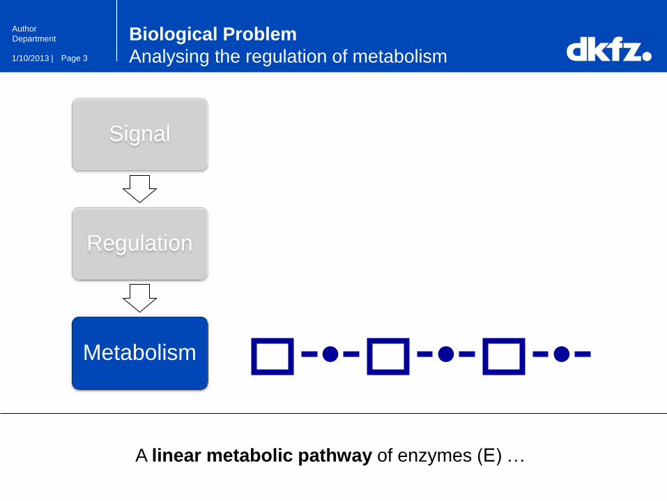
Signal

Regulation

Metabolism

A linear metabolic pathway of enzymes (E) …

Page 4 1/10/2013 |

Author

Department Biological Problem

Analysing the regulation of metabolism

Signal

Regulation

Metabolism

… is regulated by transcription factors (TF) …

Page 5 1/10/2013 |

Author

Department Biological Problem

Analysing the regulation of metabolism

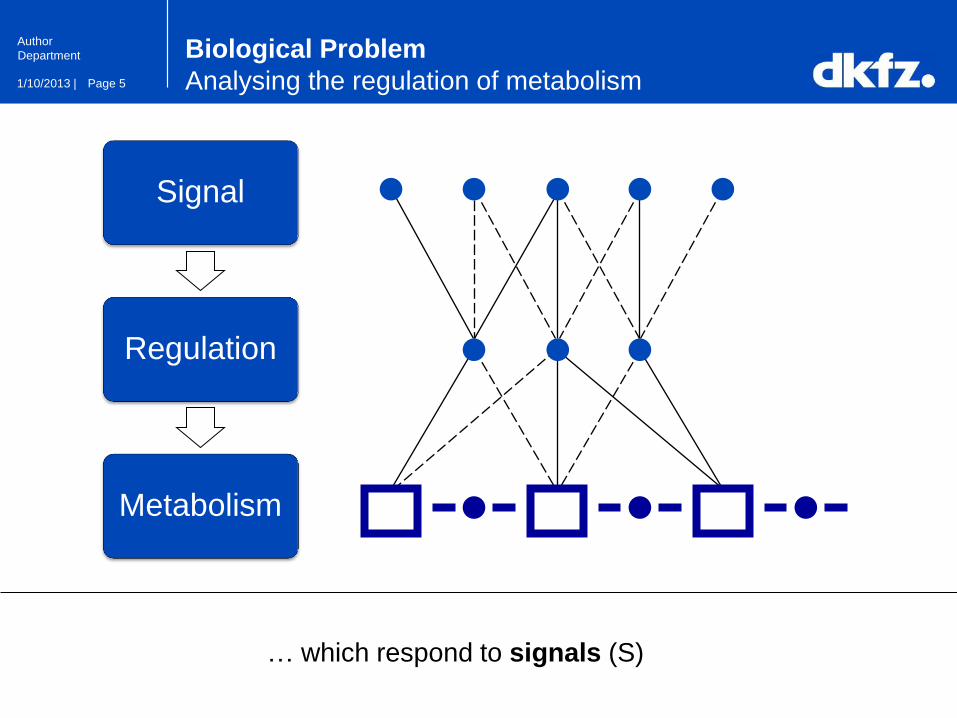
Signal

Regulation

Metabolism

… which respond to signals (S)

Page 6 1/10/2013 |

Author

Department

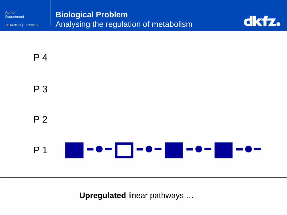
P 4

P 3

P 2

P 1

Biological Problem

Analysing the regulation of metabolism

Upregulated linear pathways …

Page 7 1/10/2013 |

Author

Department

P 4

P 3

P 2

P 1

Biological Problem

Analysing the regulation of metabolism

… can appear in different patterns

Page 8 1/10/2013 |

Author

Department Biological Problem

Analysing the regulation of metabolism

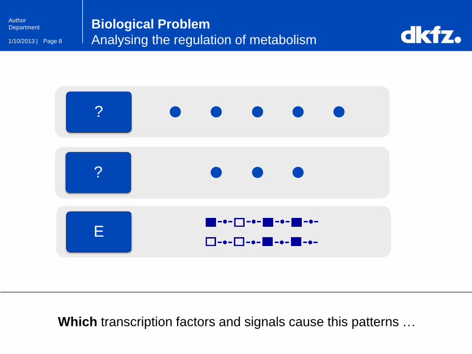
Which transcription factors and signals cause this patterns …

?

E

?

Page 9 1/10/2013 |

Author

Department Biological Problem

Analysing the regulation of metabolism

… and how do they interact? (topological structure)

?

E

?

?

?

Page 10 1/10/2013 |

Author

Department

Agenda

Biological Problem

Analysing the regulation of metabolism

Network Modeling

Restricted Boltzmann Machines (RBM)

Validation & Implementation

Page 11 1/10/2013 |

Author

Department Network Modeling

Restricted Boltzmann Machines (RBM)

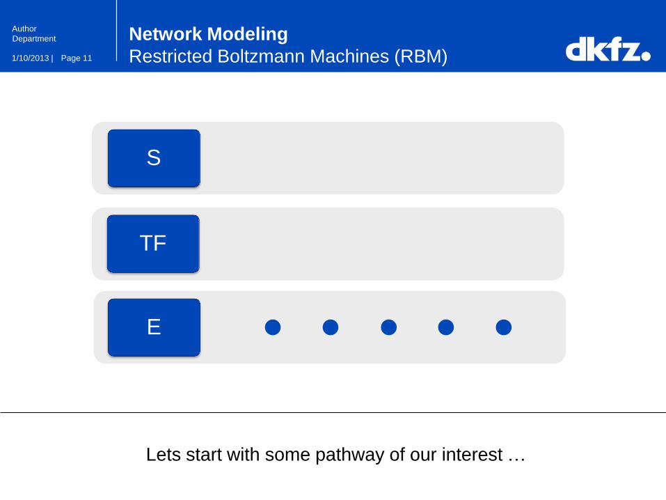
Lets start with some pathway of our interest …

S

E

TF

Page 12 1/10/2013 |

Author

Department Network Modeling

Restricted Boltzmann Machines (RBM)

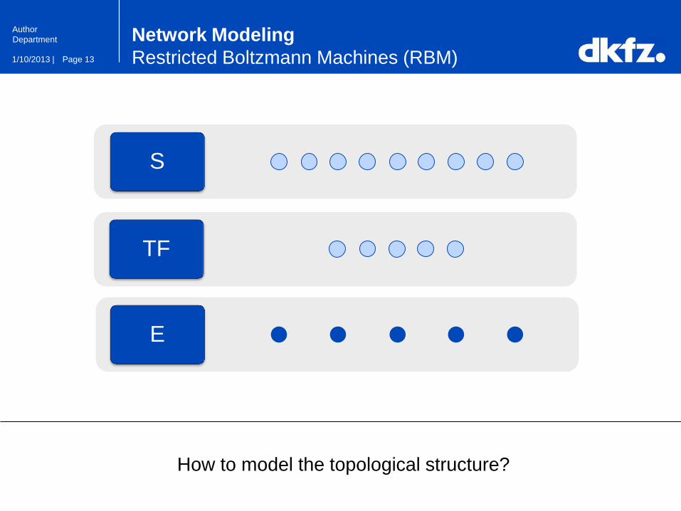
… and lists of interesting TFs and interesting SigMols

S

E

TF

Page 13 1/10/2013 |

Author

Department Network Modeling

Restricted Boltzmann Machines (RBM)

How to model the topological structure?

S

E

TF

Page 14 1/10/2013 |

Author

Department

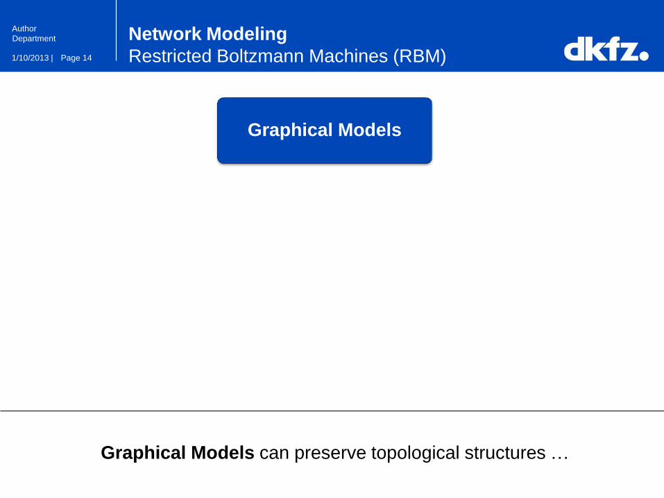
Graphical Models

Graphical Models can preserve topological structures …

Network Modeling

Restricted Boltzmann Machines (RBM)

Page 15 1/10/2013 |

Author

Department

Graphical Models

Directed Graph Undirected Graph …

… but there are many types of graphical models

Network Modeling

Restricted Boltzmann Machines (RBM)

Page 16 1/10/2013 |

Author

Department

Graphical Models

Directed Graph

Bayesian Networks Undirected Graph …

The most common type is the Bayesian Network (BN) …

Network Modeling

Restricted Boltzmann Machines (RBM)

Page 17 1/10/2013 |

Author

Department

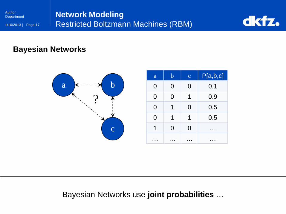
Bayesian Networks

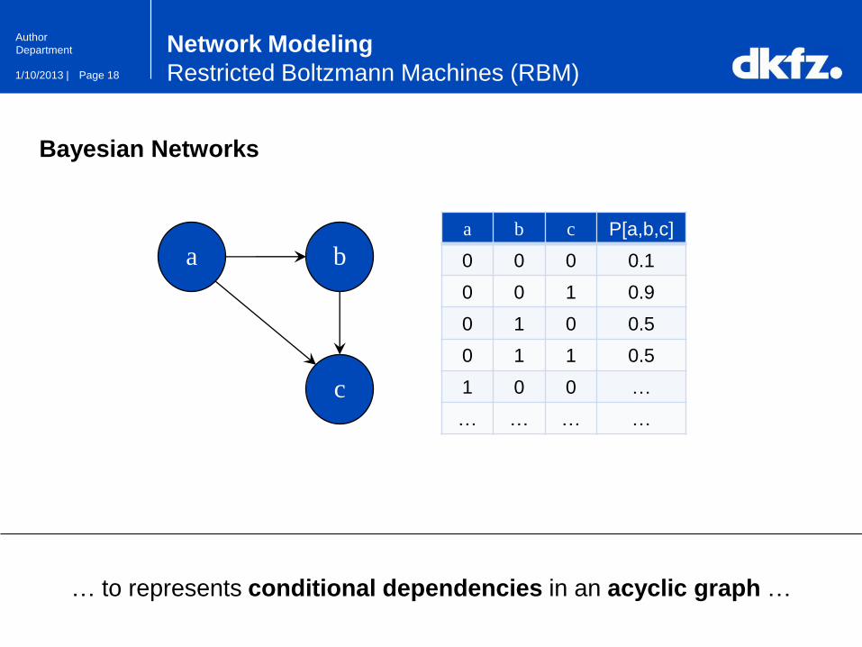
Bayesian Networks use joint probabilities …

Network Modeling

Restricted Boltzmann Machines (RBM)

a b a b c P[a,b,c]

0 0 0 0.1

0 0 1 0.9

0 1 0 0.5

0 1 1 0.5

1 0 0 …

… … … …

c

?

Page 18 1/10/2013 |

Author

Department

Bayesian Networks

… to represents conditional dependencies in an acyclic graph …

Network Modeling

Restricted Boltzmann Machines (RBM)

a b a b c P[a,b,c]

0 0 0 0.1

0 0 1 0.9

0 1 0 0.5

0 1 1 0.5

1 0 0 …

… … … …

c

Page 19 1/10/2013 |

Author

Department

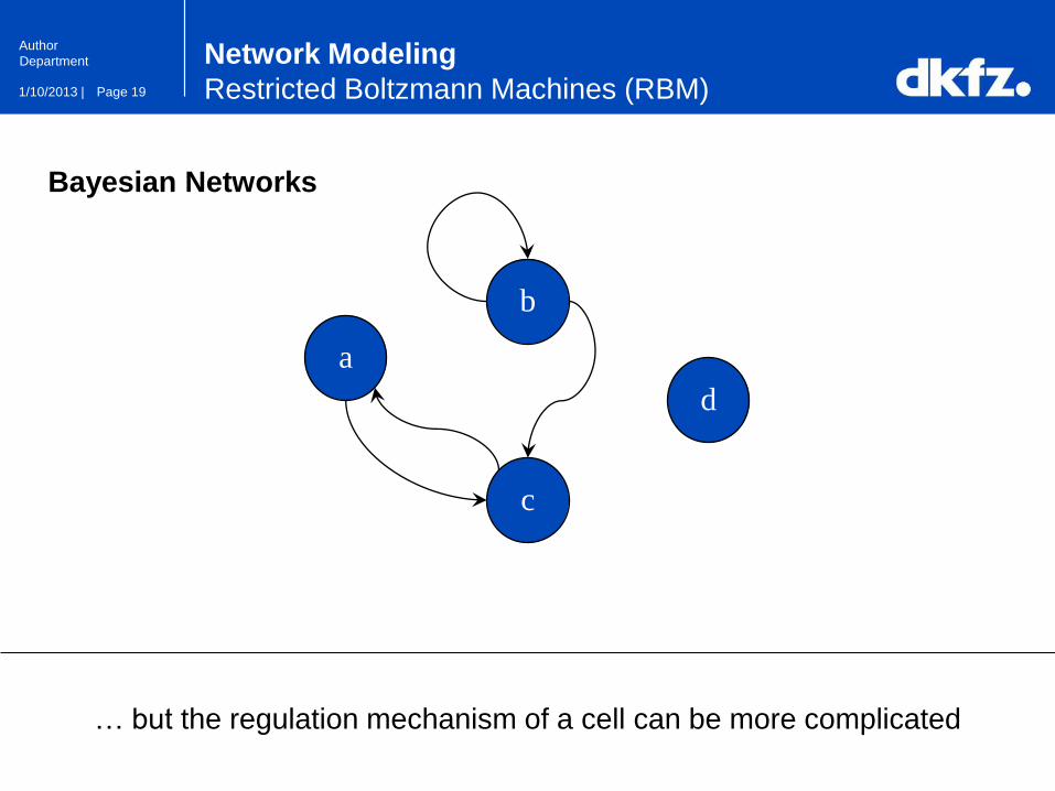
Bayesian Networks

… but the regulation mechanism of a cell can be more complicated

Network Modeling

Restricted Boltzmann Machines (RBM)

a

b

c

d

Page 20 1/10/2013 |

Author

Department

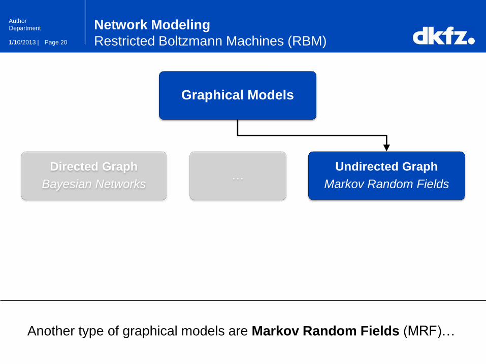
Graphical Models

Directed Graph

Bayesian Networks

Undirected Graph

Markov Random Fields …

Another type of graphical models are Markov Random Fields (MRF)…

Network Modeling

Restricted Boltzmann Machines (RBM)

Page 21 1/10/2013 |

Author

Department

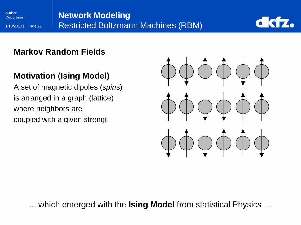
Markov Random Fields

Motivation (Ising Model)

A set of magnetic dipoles (spins)

is arranged in a graph (lattice)

where neighbors are

coupled with a given strengt

... which emerged with the Ising Model from statistical Physics …

Network Modeling

Restricted Boltzmann Machines (RBM)

Page 22 1/10/2013 |

Author

Department

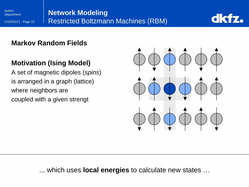
Markov Random Fields

Motivation (Ising Model)

A set of magnetic dipoles (spins)

is arranged in a graph (lattice)

where neighbors are

coupled with a given strengt

... which uses local energies to calculate new states …

Network Modeling

Restricted Boltzmann Machines (RBM)

Page 23 1/10/2013 |

Author

Department

Markov Random Fields

Drawback

By allowing cyclic dependencies

the computational costs

explode

… the drawback are high computational costs …

Network Modeling

Restricted Boltzmann Machines (RBM)

a

b

c

d

Page 24 1/10/2013 |

Author

Department

Graphical Models

Directed Graph

Bayesian Networks

Undirected Graph

Markov Random Fields

Restricted Boltzmann Machines (RBM)

…

…

… which can be avoided by using Restricted Boltzmann Machines

Network Modeling

Restricted Boltzmann Machines (RBM)

Page 25 1/10/2013 |

Author

Department

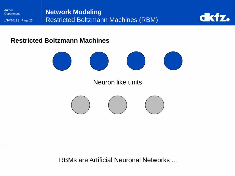
RBMs are Artificial Neuronal Networks …

Neuron like units

Network Modeling

Restricted Boltzmann Machines (RBM)

Restricted Boltzmann Machines

Page 26 1/10/2013 |

Author

Department

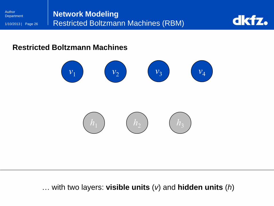
… with two layers: visible units (v) and hidden units (h)

h1

v1 v2 v3 v4

h2 h3

Network Modeling

Restricted Boltzmann Machines (RBM)

Restricted Boltzmann Machines

Page 27 1/10/2013 |

Author

Department

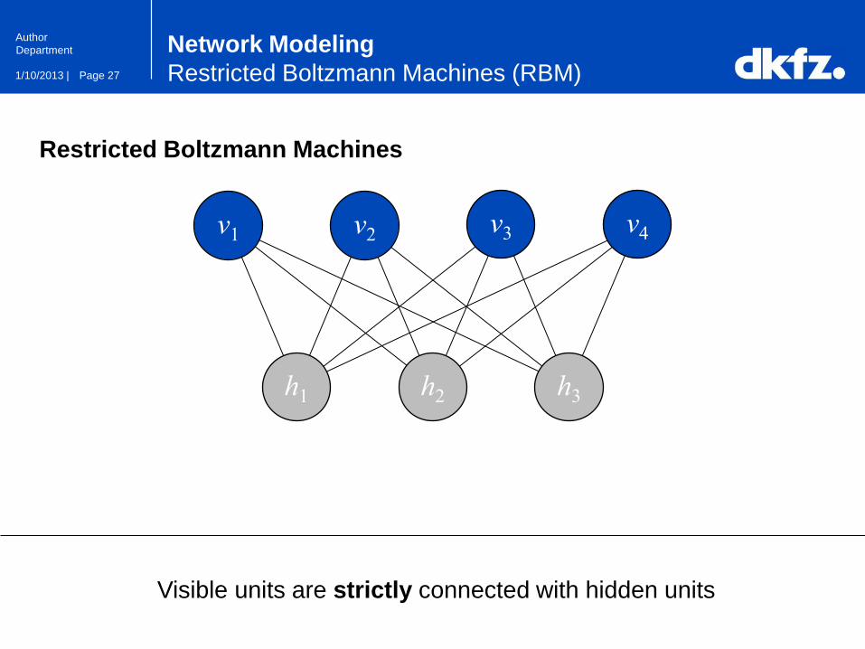
Visible units are strictly connected with hidden units

h1

v1 v2 v3 v4

h2 h3

Network Modeling

Restricted Boltzmann Machines (RBM)

Restricted Boltzmann Machines

Page 28 1/10/2013 |

Author

Department

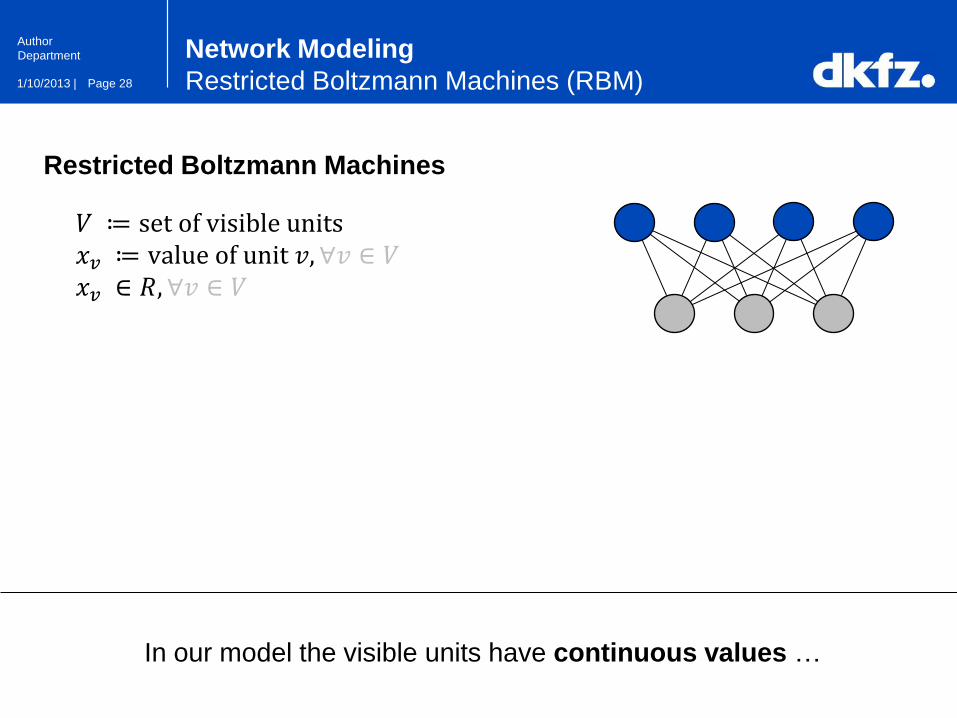
In our model the visible units have continuous values …

Network Modeling

Restricted Boltzmann Machines (RBM)

Restricted Boltzmann Machines

𝑉 ≔ set of visible units 𝑥𝑣 ≔ value of unit 𝑣, ∀𝑣 ∈ 𝑉

𝑥𝑣 ∈ 𝑅, ∀𝑣 ∈ 𝑉

Page 29 1/10/2013 |

Author

Department

… and the hidden units binary values

Network Modeling

Restricted Boltzmann Machines (RBM)

𝑉 ≔ set of visible units 𝑥𝑣 ≔ value of unit 𝑣, ∀𝑣 ∈ 𝑉

𝑥𝑣 ∈ 𝑅, ∀𝑣 ∈ 𝑉

𝐻 ≔ set of hidden units 𝑥ℎ ≔ value of unit ℎ, ∀ℎ ∈ 𝐻

𝑥ℎ ∈ {0, 1}, ∀ℎ ∈ 𝐻

Restricted Boltzmann Machines

Page 30 1/10/2013 |

Author

Department

Restricted Boltzmann Machines

Visible units are modeled with gaussians to encode data …

Network Modeling

Restricted Boltzmann Machines (RBM)

𝑥𝑣~𝑁 𝑏𝑣 + 𝑤𝑣ℎℎ 𝑥ℎ, 𝜎𝑣 , ∀𝑣 ∈ 𝑉

𝜎𝑣 ≔ std. dev. of unit 𝑣

𝑏𝑣 ≔ bias of unit 𝑣

𝑤𝑣ℎ ≔ weight of edge (𝑣, ℎ)

Page 31 1/10/2013 |

Author

Department

… and hidden units with simoids to encode dependencies

Network Modeling

Restricted Boltzmann Machines (RBM)

𝑥𝑣~𝑁 𝑏𝑣 + 𝑤𝑣ℎℎ 𝑥ℎ, 𝜎𝑣 , ∀𝑣 ∈ 𝑉

𝜎𝑣 ≔ std. dev. of unit 𝑣

𝑏𝑣 ≔ bias of unit 𝑣

𝑤𝑣ℎ ≔ weight of edge (𝑣, ℎ)

𝑥ℎ~sigmoid 𝑏ℎ + 𝑤𝑣ℎ𝑣𝑥𝑣

𝜎𝑣, ∀ℎ ∈ 𝐻

𝑏ℎ ≔ bias of unit ℎ

𝑤𝑣ℎ ≔ weight of edge (𝑣, ℎ)

Restricted Boltzmann Machines

Page 32 1/10/2013 |

Author

Department

The challenge is to find the configuration of the parameters …

Network Modeling

Restricted Boltzmann Machines (RBM)

Task: Find dependencies in data

↔ Find configuration of parameters with maximum likelihood (to data)

Learning in Restricted Boltzmann Machines

Page 33 1/10/2013 |

Author

Department

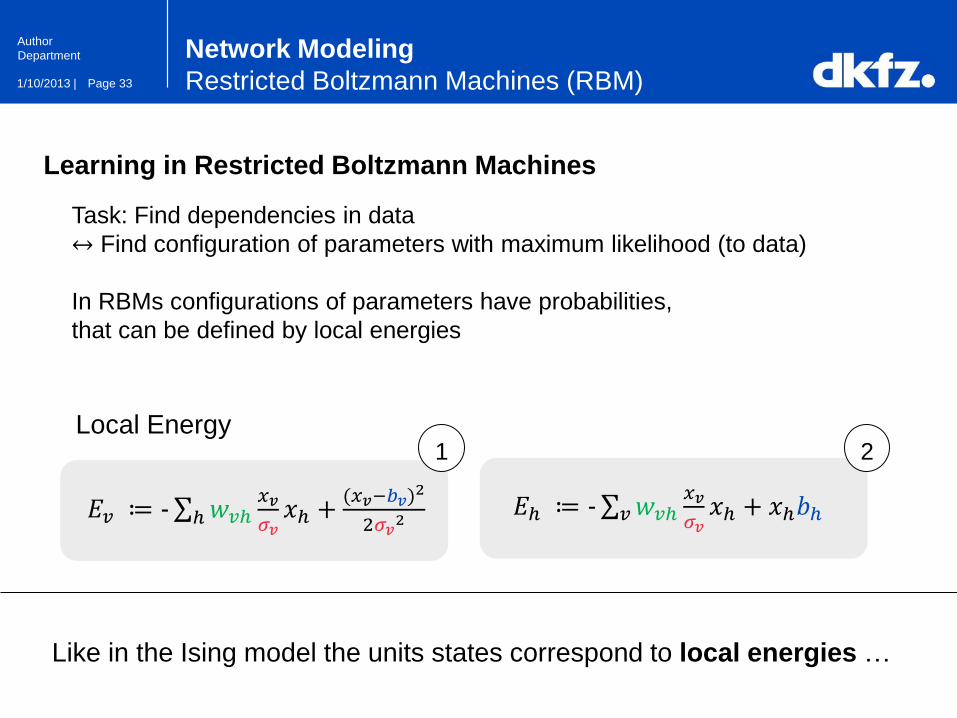
Like in the Ising model the units states correspond to local energies …

Local Energy

Network Modeling

Restricted Boltzmann Machines (RBM)

𝐸ℎ ≔ - 𝑤𝑣ℎ𝑣𝑥𝑣

𝜎𝑣𝑥ℎ + 𝑥ℎ𝑏ℎ 𝐸𝑣 ≔ - 𝑤𝑣ℎℎ

𝑥𝑣

𝜎𝑣𝑥ℎ +

(𝑥𝑣−𝑏𝑣)2

2𝜎𝑣2

Task: Find dependencies in data

↔ Find configuration of parameters with maximum likelihood (to data)

In RBMs configurations of parameters have probabilities,

that can be defined by local energies

1 2

Learning in Restricted Boltzmann Machines

Page 34 1/10/2013 |

Author

Department

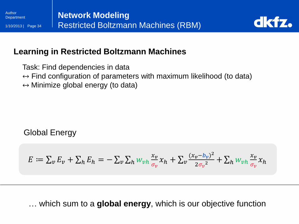
… which sum to a global energy, which is our objective function

Global Energy

Network Modeling

Restricted Boltzmann Machines (RBM)

𝐸 ≔ 𝐸𝑣𝑣 + 𝐸ℎℎ = − 𝑤𝑣ℎℎ𝑣𝑥𝑣

𝜎𝑣𝑥ℎ +

(𝑥𝑣−𝑏𝑣)2

2𝜎𝑣2 +𝑣 𝑤𝑣ℎ

𝑥𝑣

𝜎𝑣𝑥ℎℎ

Task: Find dependencies in data

↔ Find configuration of parameters with maximum likelihood (to data)

↔ Minimize global energy (to data)

Learning in Restricted Boltzmann Machines

Page 35 1/10/2013 |

Author

Department

Learning in Restricted Boltzmann Machines

The optimization can be done using stochastic gradient descent …

Network Modeling

Restricted Boltzmann Machines (RBM)

Task: Find dependencies in data

↔ Find configuration of parameters with maximum likelihood (to data)

↔ Minimize global energy (to data)

↔ Perform stochastic gradient descent on 𝜎𝑣, 𝑏𝑣, 𝑏ℎ, 𝑤𝑣ℎ (to data)

Page 36 1/10/2013 |

Author

Department

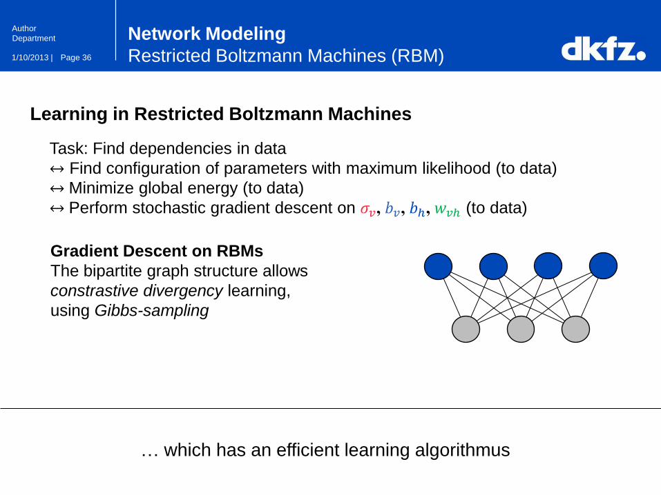
… which has an efficient learning algorithmus

Network Modeling

Restricted Boltzmann Machines (RBM)

Task: Find dependencies in data

↔ Find configuration of parameters with maximum likelihood (to data)

↔ Minimize global energy (to data)

↔ Perform stochastic gradient descent on 𝜎𝑣, 𝑏𝑣, 𝑏ℎ, 𝑤𝑣ℎ (to data)

Gradient Descent on RBMs

The bipartite graph structure allows

constrastive divergency learning,

using Gibbs-sampling

Learning in Restricted Boltzmann Machines

Page 37 1/10/2013 |

Author

Department

How to model our initial structure as an RBM?

Network Modeling

Restricted Boltzmann Machines (RBM)

S

E

TF

Page 38 1/10/2013 |

Author

Department

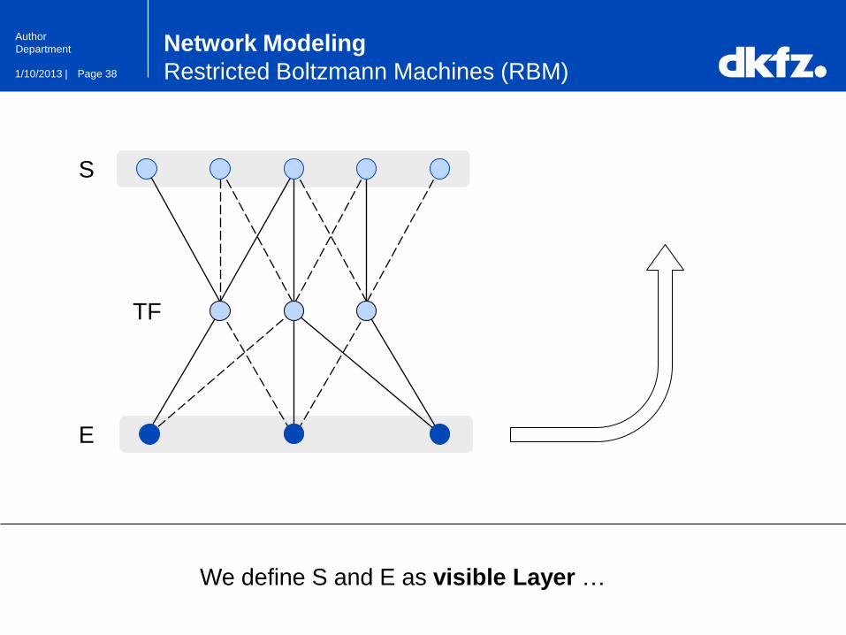
We define S and E as visible Layer …

S

E

TF

Network Modeling

Restricted Boltzmann Machines (RBM)

Page 39 1/10/2013 |

Author

Department

S E

We define S and E as visible Layer …

TF

Network Modeling

Restricted Boltzmann Machines (RBM)

Page 40 1/10/2013 |

Author

Department

S E

… and TF as hidden Layer

TF

Network Modeling

Restricted Boltzmann Machines (RBM)

Page 41 1/10/2013 |

Author

Department

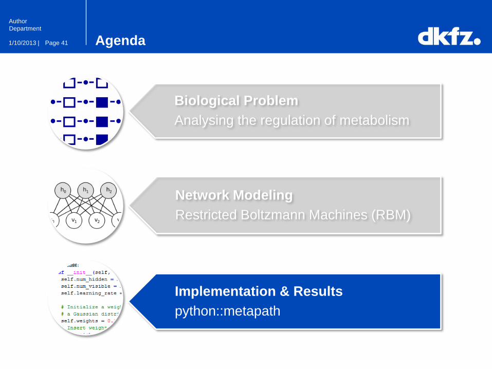
Agenda

Biological Problem

Analysing the regulation of metabolism

Network Modeling

Restricted Boltzmann Machines (RBM)

Implementation & Results

python::metapath

Page 42 1/10/2013 |

Author

Department

Results

Validation of the results

• Information about the true regulation

• Information about the descriptive power of the data

Page 43 1/10/2013 |

Author

Department

Results

Validation of the results

• Information about the true regulation

• Information about the descriptive power of the data

Without this infomation validation can only be done, using simulated data!

Page 44 1/10/2013 |

Author

Department

Results

Simulation 1

First of all we need to understand how the modell handles

dependencies and noise

To demonstrate this we create very simple data with a simple structure

Page 45 1/10/2013 |

Author

Department

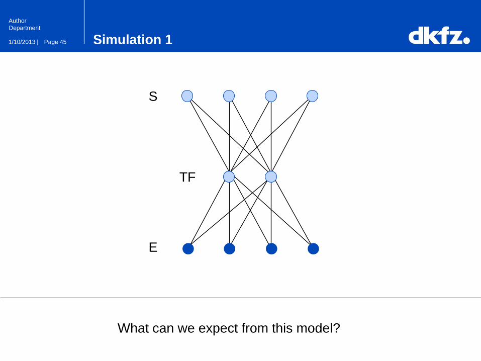
Simulation 1

What can we expect from this model?

S

E

TF

Page 46 1/10/2013 |

Author

Department

Simulation 1

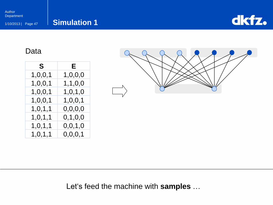
… as RBM we get 8 visible and 2 hidden units, fully connected

S E

TF

Page 47 1/10/2013 |

Author

Department

Simulation 1

Let‘s feed the machine with samples …

S E

1,0,0,1 1,0,0,0

1,0,0,1 1,1,0,0

1,0,0,1 1,0,1,0

1,0,0,1 1,0,0,1

1,0,1,1 0,0,0,0

1,0,1,1 0,1,0,0

1,0,1,1 0,0,1,0

1,0,1,1 0,0,0,1

Data

Page 48 1/10/2013 |

Author

Department

Simulation 1

.. to get the calculated parameters (especially the weight matrix)

Weight matrix

TF1 TF2

S1 0,3 0,8

S2 0,5 0,6

S3 1,0 0,1

S4 0,3 0,8

E1 0,8 0,0

E2 0,1 0,0

E3 0,1 0,0

E4 0,2 0,0

Page 49 1/10/2013 |

Author

Department

Simulation 1

The weights are visualized by the intensity of the edges

S

E

TF

TF1 TF2

S1 0,3 0,8

S2 0,5 0,6

S3 1,0 0,1

S4 0,3 0,8

E1 0,8 0,0

E2 0,1 0,0

E3 0,1 0,0

E4 0,2 0,0

Weight matrix

Page 50 1/10/2013 |

Author

Department

Simulation 1

Now we can compare the results with the samples

S E

1,0,0,1 1,0,0,0

1,0,0,1 1,1,0,0

1,0,0,1 1,0,1,0

1,0,0,1 1,0,0,1

1,0,1,1 0,0,0,0

1,0,1,1 0,1,0,0

1,0,1,1 0,0,1,0

1,0,1,1 0,0,0,1

Learning samples S

E

TF

Page 51 1/10/2013 |

Author

Department

Simulation 1

There‘s a strong dependency between S3 an E1

S E

1,0,0,1 1,0,0,0

1,0,0,1 1,1,0,0

1,0,0,1 1,0,1,0

1,0,0,1 1,0,0,1

1,0,1,1 0,0,0,0

1,0,1,1 0,1,0,0

1,0,1,1 0,0,1,0

1,0,1,1 0,0,0,1

Learning samples S

E

TF

Page 52 1/10/2013 |

Author

Department

Simulation 1

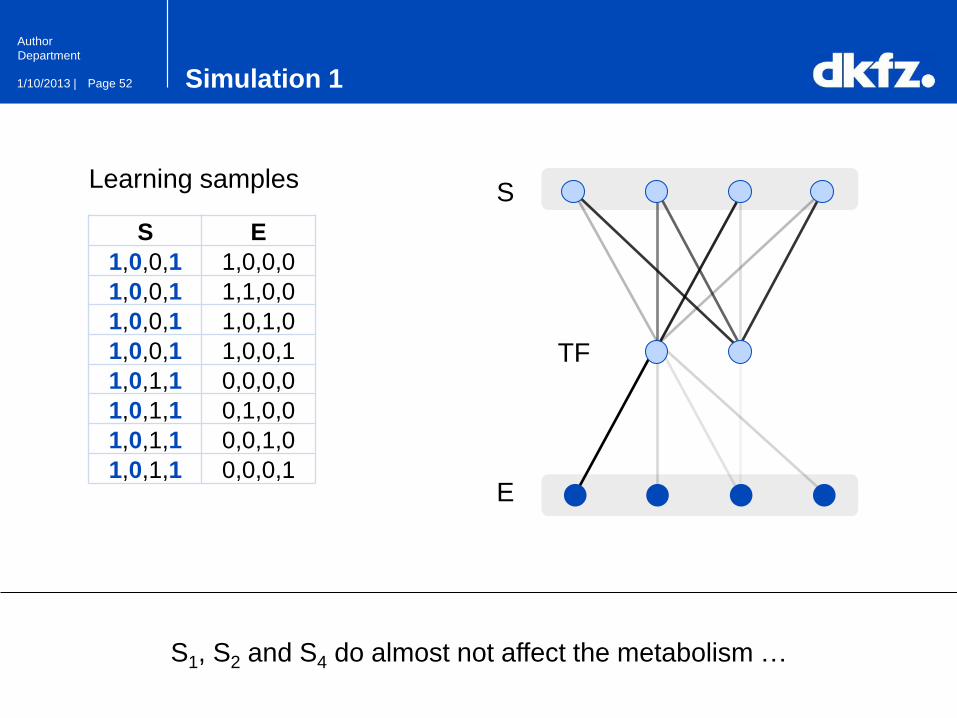
S1, S2 and S4 do almost not affect the metabolism …

S E

1,0,0,1 1,0,0,0

1,0,0,1 1,1,0,0

1,0,0,1 1,0,1,0

1,0,0,1 1,0,0,1

1,0,1,1 0,0,0,0

1,0,1,1 0,1,0,0

1,0,1,1 0,0,1,0

1,0,1,1 0,0,0,1

Learning samples S

E

TF

Page 53 1/10/2013 |

Author

Department

Simulation 1

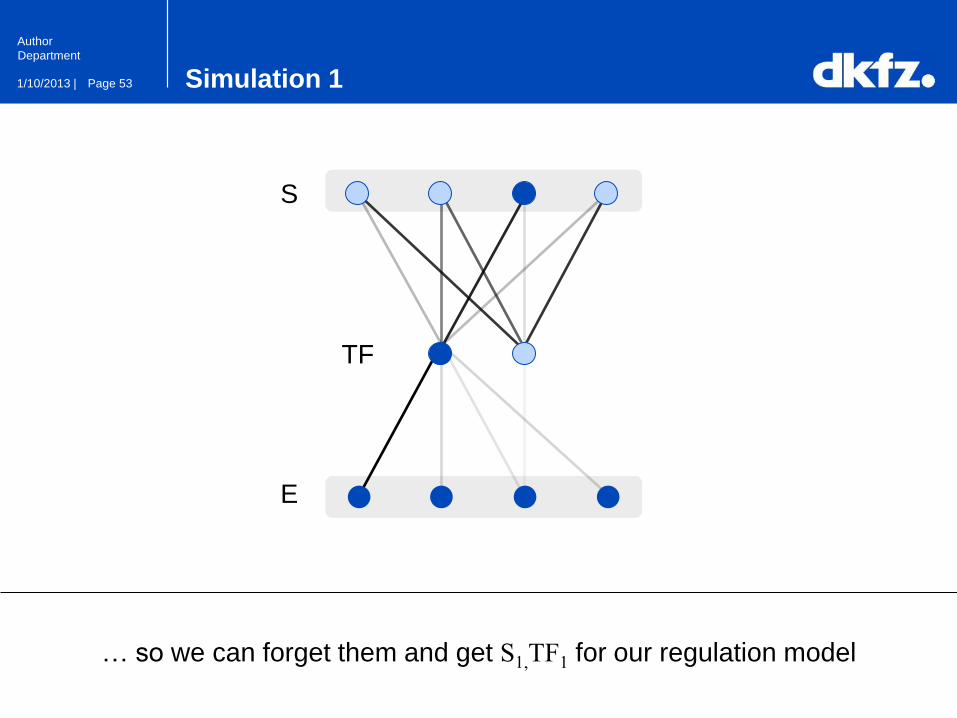
… so we can forget them and get S1,TF1 for our regulation model

S

E

TF

Page 54 1/10/2013 |

Author

Department

Simulation 1

We can also take a look at the causal mechanism …

TF1 TF2

S1 0,3 0,8

S2 0,5 0,6

S3 1,0 0,1

S4 0,3 0,8

E1 0,8 0,0

E2 0,1 0,0

E3 0,1 0,0

E4 0,2 0,0

Weight matrix

Page 55 1/10/2013 |

Author

Department

Simulation 1

The edge (S3, TF1) dominates TF1 …

TF1 TF2

S1 0,3 0,8

S2 0,5 0,6

S3 1,0 0,1

S4 0,3 0,8

E1 0,8 0,0

E2 0,1 0,0

E3 0,1 0,0

E4 0,2 0,0

Weight matrix

Page 56 1/10/2013 |

Author

Department

Simulation 1

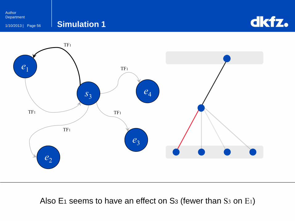
Also E1 seems to have an effect on S3 (fewer than S3 on E1)

s3

e1

e2

e3

e4

TF1

TF1

TF1

TF1

TF1

Page 57 1/10/2013 |

Author

Department

Results

Comparing to Bayesian Networks

For this purpose we simulate data in three steps

Of course we want to compare the method with Bayesian Networks

Page 58 1/10/2013 |

Author

Department

Results

Comparing to Bayesian Networks

Step 1

Choose number of Genes (E+S) and

create random bimodal distributed data

Of course we want to compare the method with Bayesian Networks

Page 59 1/10/2013 |

Author

Department

Results

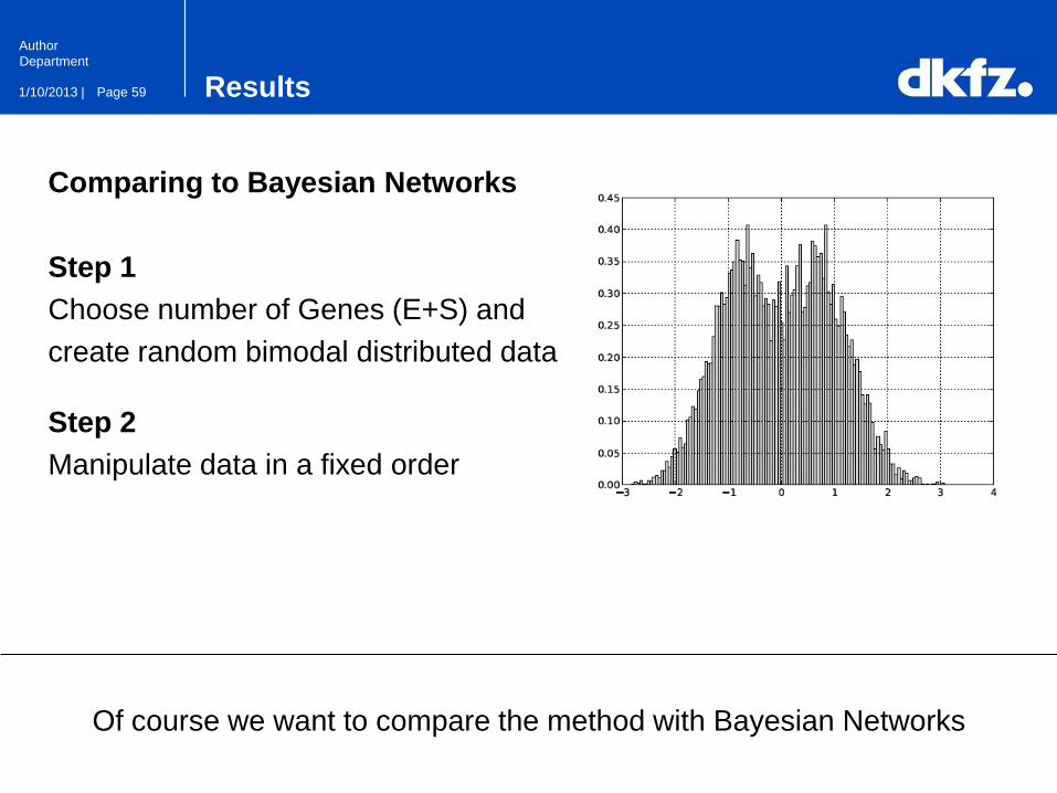
Comparing to Bayesian Networks

Step 1

Choose number of Genes (E+S) and

create random bimodal distributed data

Step 2

Manipulate data in a fixed order

Of course we want to compare the method with Bayesian Networks

Page 60 1/10/2013 |

Author

Department

Results

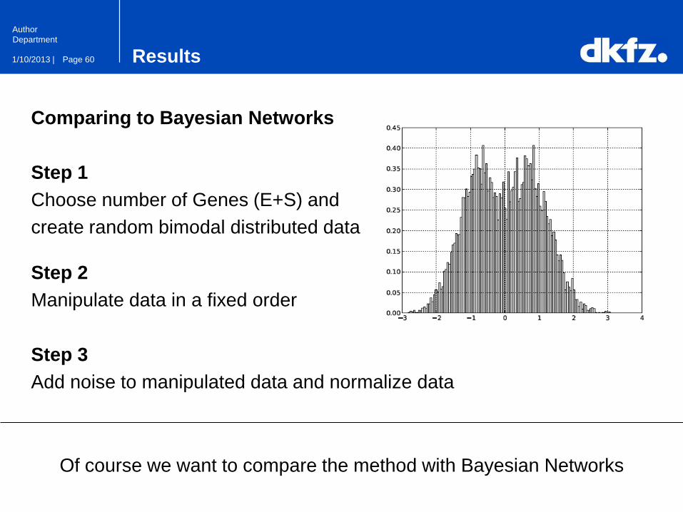
Comparing to Bayesian Networks

Step 1

Choose number of Genes (E+S) and

create random bimodal distributed data

Step 2

Manipulate data in a fixed order

Step 3

Add noise to manipulated data and normalize data

Of course we want to compare the method with Bayesian Networks

Page 61 1/10/2013 |

Author

Department

Results

Comparing to Bayesian Networks

Idea

• ‚melt down‘ the bimodal distribution from very sharp to very noisy

• Try to find the original causal structure with BN and RBM

• Measure Accuracy by counting the right and wrong dependencies

Of course we want to compare the method with Bayesian Networks

Page 62 1/10/2013 |

Author

Department

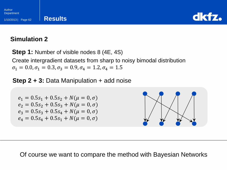
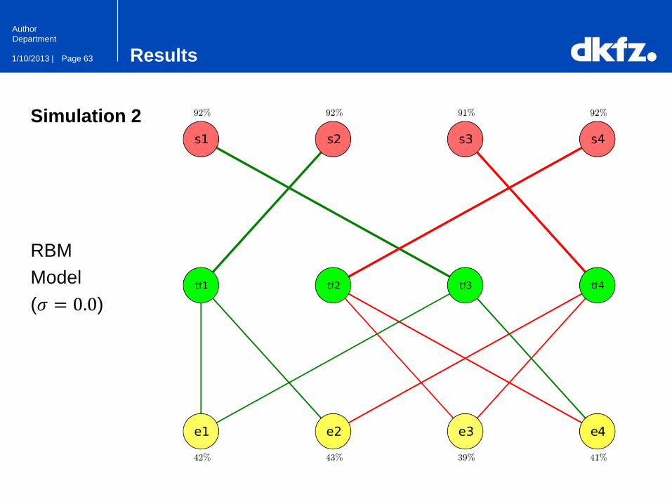
Simulation 2

Results

𝑒1 = 0.5𝑠1 + 0.5𝑠2 + 𝑁(𝜇 = 0, 𝜎) 𝑒2 = 0.5𝑠2 + 0.5𝑠3 + 𝑁(𝜇 = 0, 𝜎) 𝑒3 = 0.5𝑠3 + 0.5𝑠4 + 𝑁(𝜇 = 0, 𝜎) 𝑒4 = 0.5𝑠4 + 0.5𝑠1 + 𝑁(𝜇 = 0, 𝜎)

Of course we want to compare the method with Bayesian Networks

Step 1: Number of visible nodes 8 (4E, 4S)

Create intergradient datasets from sharp to noisy bimodal distribution

𝜎1 = 0.0, 𝜎1 = 0.3, 𝜎3 = 0.9, 𝜎4 = 1.2, 𝜎4 = 1.5

Step 2 + 3: Data Manipulation + add noise

Page 63 1/10/2013 |

Author

Department

Results

Simulation 2

RBM

Model

(𝜎 = 0.0)

Page 64 1/10/2013 |

Author

Department

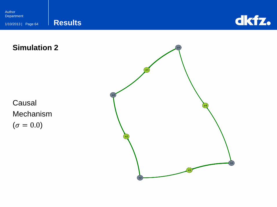
Results

Simulation 2

Causal

Mechanism

(𝜎 = 0.0)

Page 65 1/10/2013 |

Author

Department

Results

Simulation 2

Comparison

BN / RBM

0

0,2

0,4

0,6

0,8

1

1,2

RBM

BN

Page 66 1/10/2013 |

Author

Department

Conclusion

Conclusion

• RBMs are more stable against noise compared to BNs.

It has to be assumed that RBMs have high predictive power regarding

the regulation mechanisms of cells

• The drawback are high computational costs

Since RBMs are getting more popular (Face recognition / Voice

recognition, Image transformation). Many new improvements in facing

the computational costs have been made.

Page 67 1/10/2013 |

Author

Department

Acknowledgement

eilsLABS

PD Dr. Rainer König

Prof. Dr Roland Eils

Network Modeling Group