1

Relationship between Remittances and Macroeconomic

variables in an Unstable Context: Evidence from

Tunisia‟s Arab Spring†

Jamal BOUOIYOUR (CATT, University of Pau)

‡

Refk SELMI (University of Tunis)

Amal MIFTAH (LEDa, University of Paris-Dauphine)

Abstract: Regardless of its progress and regional success story, the onset of the so-

called “Arab Spring” unveiled economic weaknesses previously masked by economic

and political stability. Nowadays, the political and social unrest underscores the

fragility of the pillars of Tunisia‟s growth; the tourism collapsed, the dinar depreciated,

the demand of exports dwindled and the foreign direct investment grew less.

Exceptionally, due to its countercyclical behavior, remittances were resilient in dealing

with this shock. This paper employs a new data analysis tools to address whether

remittances may simultaneously spur economic growth, stabilize consumption

fluctuations and stimulate productive investment. These techniques contain several

novel features that set this study apart from the literature on the issue. Our results

reveal that, prior to the Arab Spring, the remittance‟ impact on growth was negative,

while its effect on consumption was significantly positive. However, remittances

varyingly influenced local investment. These three relationships were supported in the

short-run. By considering the period surrounding the 2011 uprisings, the investment

effect of remittance inflows became negative, weak and determined by short- and

medium-term factors, whereas a positive, strong and long-term remittances‟ impacts

on growth and consumption were shown. Overall, in an unstable context, remittances

were found to be driven by the need to support migrant worker‟s families rather than

by investment considerations.

Keywords: Remittances; growth; investment; consumption; Tunisia; Arab Spring.

JEL Codes: F24; E6.

†The content of this paper has been presented at the annual seminar of ESC Pau and the 4th

TMENA meeting. We are highly indebted to the participants for helpful and constructive

comments. ‡ Corresponding author : jamal.bouoiyour@univ-pau.fr

Full address: Avenue du Doyen Poplawski, 64016 Pau Cedex, France; Phone: 33 (0)5 59 40

80 01; Fax: 33 (0)5 59 40 80 10

2

1. Introduction

Around noon on 17 December 2010, young Tunisian street merchant, Mohamed

Bouazizi lit the fuse that ended his life and exacerbated unrest sweeping in Tunisia.

His suicide was seen as an act of defiance against the government and frustration

confronted by the majority of Tunisians: the widespread corruption, the inequality and

the crippling poverty. The winds of change that swept across Tunisia triggered a

“domino” effect in different Arab countries including Egypt, Libya, Syria and Yemen,

among others. These revolutions had incited what we call the “Arab Spring”.

Following the euphoria of the event, Tunisia experienced an evolving volatility and

growth slow-moving. In retrospect, before the downfall of Ben Ali who had ruled the

country with its authoritarian regime for 23 years, Tunisia had been praised by

international organizations as an example. It has long been perceived as one of the

widely cited development success stories in the Middle Eastern and North African

region, and was portrayed as a “top reformer” as far as institutional reform was

concerned (Pollack 2011). Tunisia‟s economic growth in 2011 was expected to exceed

5 percent, outpacing low-middle-income countries‟ averages. It has also succeeded to

keep its domestic and external economic imbalances under control; thanks to the 1986

structural adjustment program and the macro-economic improvement called „economic

miracle” beginning in the late 1990s. However, issues of youth unemployment,

corruption and unequal wealth distribution have received much less attention. It comes

as no surprise that popular uprising occurs in such framework. In fact, despite a

marked economic progress, the system cannot stay without real democracy and

equitable wealth distribution.

One of the main economic consequences of the Arab Spring was the sharp

decrease of the annual growth: 1 percent per year between 2011 and 2015. Further, the

Tunisia‟s economy struggled with widespread unemployment coupled with the

fragility of the pillars of Tunisia‟s growth; According to the National Institute of

Statistics of Tunisia, the foreign direct investment (FDI) plunged by 7.6 percent in

2016 compared to 2010. The unemployment rate attained almost 15.5 percent in 2016.

The inflation rate increased of approximately 3.9 percent. The current account deficit

3

attained in 2015 almost 8.5 percent. The trade deficit rose markedly to reach 13.6

percent of GDP. Also, Tourist arrivals and revenues collapsed by 30.8 and 35.1

percent, respectively, and the dinar depreciated substantially.

To address the country‟s challenges, there is a need for considering counter-

cyclical financing mechanisms and other pillars for economic development. Among

these relays, migrant‟ remittances may help to cushion the harmful effects of this

political and social upheaval. In fact, in times of crises (2008 and 2011), remittance

flows showed a resilience (World Bank 2012). Nevertheless, these financial flows had

not attracted so much attention from successive governments, unlike other recipient

countries such as Morocco where these funds have been and are still being one of the

major sources of financing the economy (Bouoiyour 2006).

The present study assesses whether remittances may boost economic

development, stabilize consumption fluctuations and stimulate investment activities,

by delving into the case of Tunisia witnessing the 2011 Arab Spring unrest. While a

large strand of literature has focused on how remittance inflows interact with

economic growth and investment (El-Sakka and Mcnabb 1999, Glystos 2002,

Amuedo-Dorantes and Pozo 2004, Fayissa and Nsiah 2008, Yang 2008, Tansel and

Yasar 2009, Barajas et al. 2009), very little was devoted in the literature to the

stabilizing effects of remittances on consumption variations (Bhaumik and Nugent

1999, Kedir and Girma 2003, Castaldo and Reilly 2007). Also, a limited number of

studies has analyzed the ability of remittances to act as a buffer against shocks (Lueth

and Ruiz-Arranz 2007, Chami et al. 2005). This paper extends previous literature in

the following important aspects. First, it simultaneously examines the remittances‟

impacts on economic growth, domestic investment and consumption. Second, it tries

to identify through which channels remittances can spur Tunisia‟s growth during

turbulent times. Third, because it is not easier to analyze the linkage between

remittances and the macroeconomy over the ongoing uncertainty surrounding Tunisia

in the aftermath of Arab Spring, the use of newly data analyses may be very useful. A

review of the literature on the central issue suggests the existence of an intricate

relationship remittances and macroeconomic variables. This may be due to the fact

that the majority of these studies use conventional models such as OLS, VECM and

4

VAR. Hence a novel econometric tool is necessary to obtain fresh insights into this

inconclusive topic. In brief, this study underscores the relevance to decompose

processes into individual components and examine each of the components separately,

and thus to analyze how evolve the relationship between remittances and the

macroeconomy over different frequency components (short-, medium- and long-run).

In particular, we carry out new techniques permitting the analysis with respect to

frequency, namely empirical mode decomposition (EMD) and frequency domain

causality. The EMD, initiated by Huang et al. (1998), gives fresh insights in situations

where other methods fail. It has proven to be appropriate in a broad range of

applications for extracting signals from data generated in noisy nonlinear and non-

stationary processes (for instance, Huang and Attoh-Okine 2005; Bouoiyour et al.

2016). Moreover, instead of computing a Granger causality measure for the entire

relationship between remittances and macroeconomic variables, as it is usually done,

this paper deals with the links remittances-economic growth, remittances-consumption

and remittances-investment in Tunisia for each individual frequency separately using a

frequency domain causality test first developed by Breitung and Candelon (2006).

The correlation analysis-based EMD gathered quite interesting results. Prior to

Arab Spring, the short-term hidden factors of remittances explain negatively the

economic growth, varyingly the local productive investment and positively the

consumption. These results change fundamentally when accounting for the period

surrounding Tunisia in the onset of Arab Spring. While the findings remain stable for

the remittances-investment linkage (negative and weak and driven by short- and

medium-term factors), the cycles remittances-growth and remittances-consumption

became positive, greater and explained by long-term inner features. These results are

robust to the control for endogeneity bias. In addition, the findings of frequency

domain causality test go in the same direction with respect the consistency of the

cycles between the variables of interest. In a nutshell, this article‟ outcomes deeply

suggest that the remittance flows, in turbulent times, were shown to be spent more on

consumption and less on domestic investments.

5

The outline of the paper is as follows. Section 2 presents a literature review on

the channels through which remittances can enhance economic growth in the

developing countries. Section 3 gives some stylized facts. Section 4 discusses the

methodology and provides a brief data overview. Section 5 reports and discusses our

results. Section 6 checks the robustness and the consistency of our results. The last

section (Section 7) concludes and offers some policy implications.

2. Literature review

Theoretical literature has underscored various channels through which migrant

remittances can spur economic growth in the developing countries. However, it has

proven not easier to incontrovertibly support the idea that remittances provide a boost

to economic growth of recipient economies, and whether they help lighten economic

hardship. Concerning this point, remittances can mitigate output growth volatility

because of their relative stability. Some papers argued that remittances may act as a

countercyclical stabilizer in receiving countries. For example, Chami et al. (2005)

indicated that remittances have a tendency to move counter-cyclically with the GDP in

recipient countries, consistently with the model‟s implication that remittances are

compensatory transfers. However, Lueth and Ruiz-Arranz (2007) found that

remittance receipts in Sri Lanka may be less shock-absorber than usually believed.

A limited strand of literature which has tested the direct relationship between

remittances and economic growth typically showed “multi-sided” outcomes.

Estimating panel growth regressions both on the full sample of countries (composed of

84 countries) and for emerging economies only, Barajas et al. (2009) claimed that

remittances had, at best, no impact on economic growth. Fayissa and Nsiah (2010)

investigated the aggregate impact of remittances on the economic growth of 18 Latin

American countries for the period 1980–2005 and showed that a 10 percent increase in

remittances led to a 0.15 percent increase in the GDP per capita income. Using the

Solow growth model, Rao and Hassan (2009) explained the impacts of remittances on

growth by distinguishing between the indirect and direct growth effects of remittances.

They found that migrants‟ remittances were likely to have a positive but modest effect

6

on economic growth. These authors identified seven channels through which

remittances could have indirect growth effects: the volatility of output growth, the

exchange rate, the investment rate, the financial development, the inflation rate, the

foreign direct investment and the current government expenditure. To a larger extent,

the surveyed literature suggested different channels through which remittances could

spur economic growth. In the short-run, remittances allowed home countries to

strengthen the foreign-exchange reserves helping to adjust their macroeconomy.

Nevertheless, the rather extensive literature on remittances provided further insights on

the effects of remittances on consumption and investment (El-Sakka and Mcnabb

1999; Glytsos 2002). Accordingly, for a sample of five Mediterranean countries

(namely Egypt, Greece, Jordan, Morocco and Portugal), Glytsos (2002) analyzed the

remittances‟ impacts on growth, and deduced that the good done to growth by rising

remittances is not as great as the bad done by falling remittances.

From an economic development viewpoint, a vexing question remains: how

remittances are used. Are they spent on consumption, or are they used for productive

investments? Remittances are generally spent on consumption but there is some

evidence that in the long term international remittances may be channelled into

productive investment. In this context, some studies looked into the effects of

remittances on domestic investment (and hence indirectly on growth) and supported

these optimistic conclusions. For example, Woodruff and Zenteno (2004) analyzed

such effects using data of a survey of more than 6,000 self employed workers and

small firm owners located in 44 urban areas of Mexico and estimated that more than

40 percent of the capital invested in microenterprises in urban Mexico was associated

with migrants‟ remittances. There is also evidence supporting that return migration

could increase investment in some developing countries like Egypt (McCormick and

Wahba 2003 and Wahba and Zenou 2009) and Tunisia (Mesnard 2004). Potentially,in

countries where access to credit is a major obstacle for entrepreneurship, return

migration invigorated the propensity of returnees to become self-employed upon return

but also the positive impact of accumulated savings on the decision to become self-

employed. Additionally, it has been commonly argued that investment is directly

7

linked to the development of financial system (Aggarwal et al 2006, Giuliano and

Ruiz-Arranz 2009).

There are other channels through which remittances could affect growth,

namely human capital and labor supply. With regard to human capital, remittances can

stimulate investment in human capital and health as well (Mansuri 2006, Valero-Gil

2008). Remittances may also influence economic growth via their effects on the labor

force participation. However, the effects of remittances on labor force participation are

sensitive to the considered countries. Some migration research showed that

remittances flows negatively influenced labor supply if remittance income substitutes

for labor income. They had also a disincentive impact on work and savings in the

origin community of migrants i.e., the moral hazard phenomenon (Chami et al. 2005),

leading to a decrease of labor supply. Nevertheless, as noted by Özden and Schiff

(2006), the decline in labor supply caused by remittances may prompt high

productivity.

3. Migration flows and remittances to Tunisia

Migrants from Tunisia are predominantly destined for Europe, and for historical

and political reasons, France has attracted the majority of the Tunisian community

abroad. According to the official data, 1,223,213 Tunisians (i.e. 10 percent of the

Tunisian population) were residing abroad in 2012, more than 1 million of whom lived

in Europe (668,668 in France). If Tunisian migration flows to traditional European

countries like France and Germany have increased during the last decades due to

family reunification, the migration to other destination countries is explained by labour

migration. This is the case for example of the migration to Gulf countries which is

generally temporary. These migration flows respond to economic and political

backgrounds in Tunisia and in host countries. In recent years, high unemployment and

political instability in the country can be viewed as the major cause of the decision to

emigrate. The official data suggest that in 2012, graduate unemployment rates (tertiary

education level), in Tunisia, stood at 26.1 percent. Unemployment represents a drama

in the lives of many young individuals in this country and could be one of the most

important reasons of their emigration. The high skilled emigration had also grown

8

significantly over the past two decades, reflecting the selective nature of migration by

educational attainment and the general improvement in the level of education in this

country. Looking at the OECD data about the emigration rate of the highly educated

persons ††

in 2010-2011, Tunisia has almost 10 percent of its skilled workforce living

abroad (OECD 2013). Note that during the time of the revolution, there was a

significant increase of irregular migration flows towards Europe. A prominent feature

linked to Tunisian migration is the increasing volume of remittances sent by

international migrants. They registered a noticeable increase during the two last

decades. In 1990, international remittances received were around $0.5 billion; by

2008, this number rose to $1.9 billion. In 2014, they attained $2.35 billion. These

official statistics reported by the Central Bank of Tunisia largely underestimate the

total amount of migrants‟ remittances because Tunisian migrants frequently used

informal modes of transfer. In Tunisia, informal remittances carried by travellers from

Europe (migrants, family, friends and acquaintances) were estimated to account for 38

percent of total remittance receipts (IOM report, 2011).

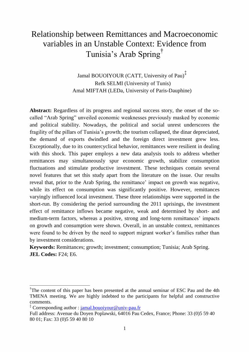
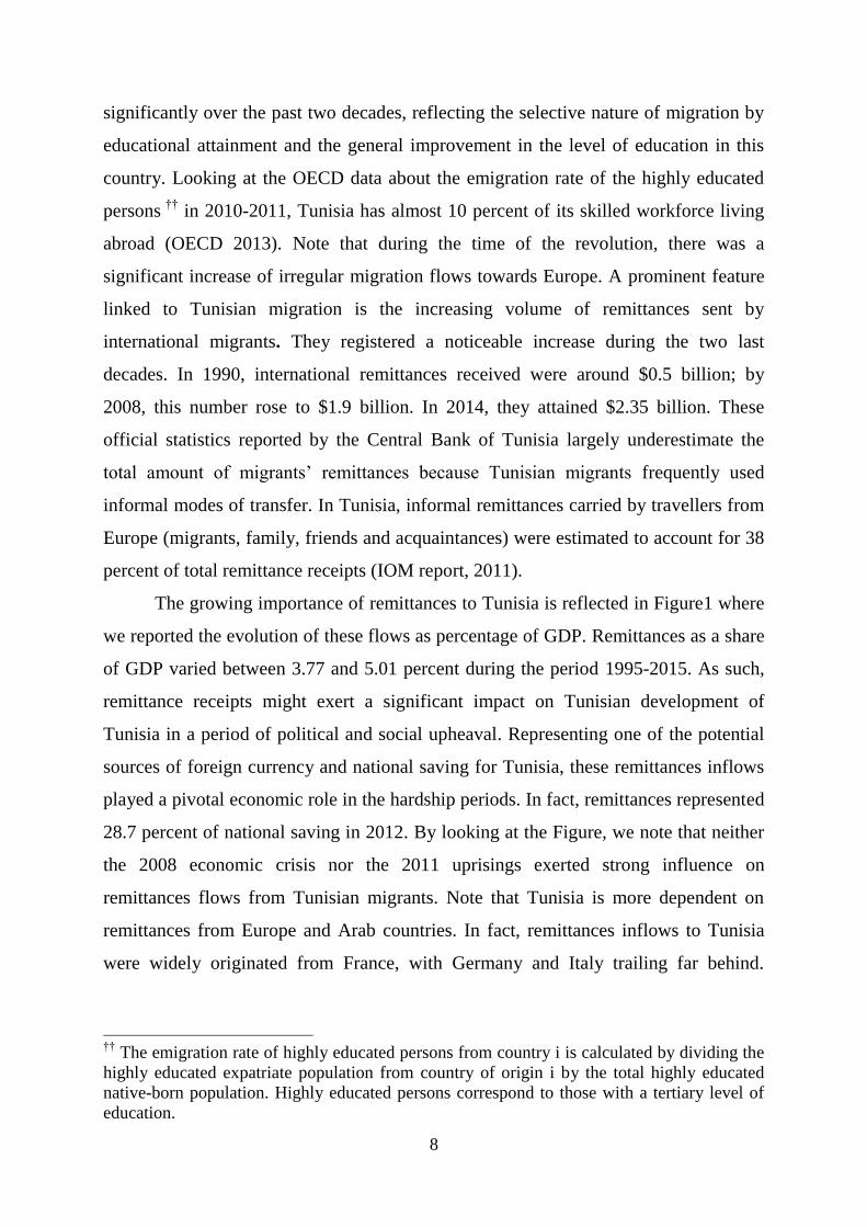
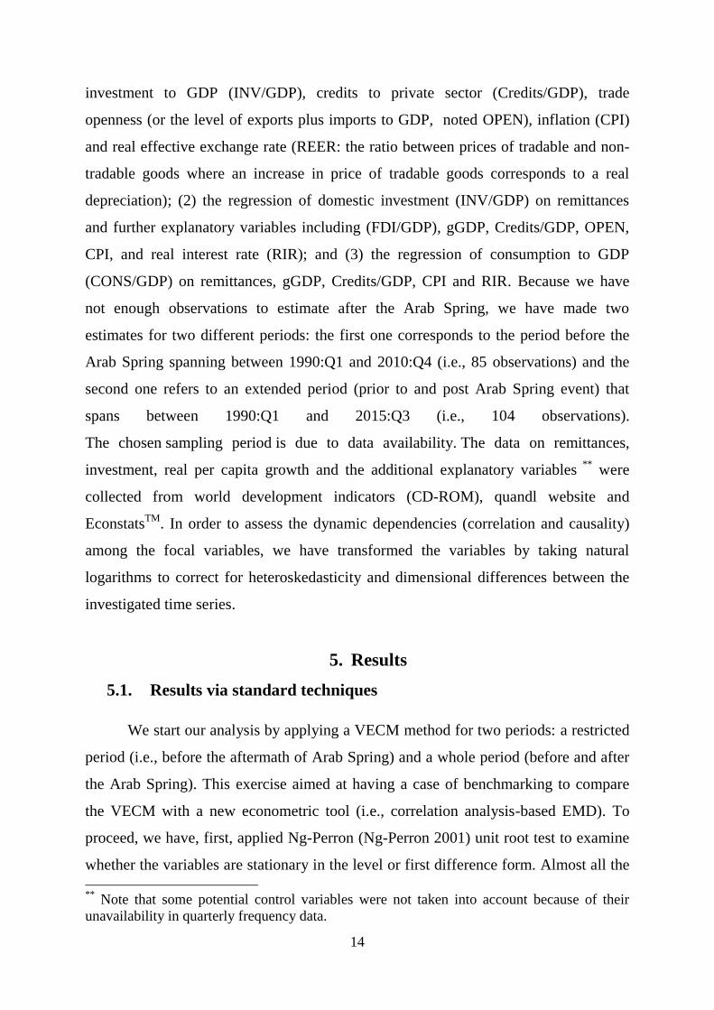
The growing importance of remittances to Tunisia is reflected in Figure1 where

we reported the evolution of these flows as percentage of GDP. Remittances as a share

of GDP varied between 3.77 and 5.01 percent during the period 1995-2015. As such,

remittance receipts might exert a significant impact on Tunisian development of

Tunisia in a period of political and social upheaval. Representing one of the potential

sources of foreign currency and national saving for Tunisia, these remittances inflows

played a pivotal economic role in the hardship periods. In fact, remittances represented

28.7 percent of national saving in 2012. By looking at the Figure, we note that neither

the 2008 economic crisis nor the 2011 uprisings exerted strong influence on

remittances flows from Tunisian migrants. Note that Tunisia is more dependent on

remittances from Europe and Arab countries. In fact, remittances inflows to Tunisia

were widely originated from France, with Germany and Italy trailing far behind.

††

The emigration rate of highly educated persons from country i is calculated by dividing the

highly educated expatriate population from country of origin i by the total highly educated

native-born population. Highly educated persons correspond to those with a tertiary level of

education.

9

Among Arab countries, the Gulf Cooperation Council countries (GCC)‡‡

were the

main remittances sending countries followed by Libya before the Arab Spring which

caused a marked decline of remittances sent from Libya.

Figure 1. Remittances to Tunisia

Source: World Bank.

4. Methodology and data

The empirical investigation of the relationship between remittances and

macroeconomic variables has often been explored on the entire period generally

through OLS, VECM model and standard Granger causality test etc. These techniques

assume that the link among time series is constant throughout the period. We cannot

ascertain that this finding is absolutely true since, in practice, each relationship may

vary from one period to another. To avoid this limit, the decomposition of the

‡‡

Within the GCC region, the main remittances sending countries in 2013 were the Saudi

Arabia and the United Arab Emirates (Central Bank of Tunis 2014).

10

evolution of economic phenomena into different frequency components helps to

adequately judge how evolves such “complex” relationship over time especially in an

unstable context. So, the core focus is to suggest new techniques permitting the

investigation with respect to frequency, namely empirical mode decomposition and

frequency domain causality.

4.1. Empirical Mode Decomposition

All real processes we have to deal practically seem very complex, consisting of

an important number of components. When examining, for instance a weather chart,

we shouldn‟t overlook that such chart represents a connectedness among several

processes including seasonal changes, dynamics of cyclones and anticyclones, solar

cycles, etc. The interaction of these components may mask the regularities we would

like to identify. There is no exception when it comes to information on investment,

trading and the whole economy that are also driven by multiple hidden factors. That is

why an upfront breakdown into separate constituent components can allow for a deep

analysis of data permitting to identify inner features determining such convoluted

phenomenon.

There exist several decomposition methods that can be carried out to a given

sequence. Amongst well known decomposition approaches, one can cite the Fourier

transform. This latter belongs to the class of orthogonal transformations that uses fixed

harmonic basis functions. The Fourier transform finding can be found as a

decomposition of the initial process into various harmonic functions but with fixed

frequencies and amplitudes. Precisely, the amplitude and the frequency values of the

derived harmonic components are constant. This implies that if the behavior of a given

sequence changes during a specific period, such changes will not be adequately

reflected in the transform outcomes. Unlike the Fourier transform, every component

resulting from a wavelet transform has parameters that determine its scale and level

over time which avoids the possible non-stationarity problem. But for empirical aims,

it would be more effective to have a transform that would not only enable to deal with

non-stationarity problem but would carry out an adaptive transform basis. According

11

to Huang et al. (1998)‟s study, Fourier transform and wavelets might lead to inaccurate

information about nonlinear and non-stationary variables. To reach complete

information from signals that might be inner when employing the previous techniques,

the Empirical mode decomposition (EMD) method may be very useful. With this

technique, a complicated signal can be adaptively disentangled into a sum of finite

number of zero mean oscillating components having symmetric envelopes defined by

the local maximal and minima respectively, dubbed Intrinsic Mode Functions (IMF).

The latter serves as the basis functions, which are driven by the signal itself rather than

pre-determined kernels (Lei et al. 2013). This novel method is valuable to assess non-

linear and non-stationary signals. The EMD is based on the sequential extraction of

energy associated with distinct frequencies ranging from high fluctuating components

(short-run) to low fluctuating modes (long-run). With the Hilbert transform, the IMF

prompts instantaneous frequencies as functions of time that help to properly identify

imbedded structures. These functions should be symmetrical with respect to local zero

mean, and should have the same numbers of extrema and zero-crossings. By exploring

data intrinsic modes, the EMD aims at transforming the time series to hierarchical

structure by means of the scaling transformations. In other words, it quantifies the

changeability captured via the oscillation under different scales and locations.

Basically, the IMFs are decomposed by determining the maxima and minima of time

series )(tx , generating then its upper and lower envelopes )(( min te and )(max te ), with

cubic spline interpolation. For this purpose, we initially measure the mean )(tm for

different points from upper and lower envelopes:

2/))()(()( maxmin tetetm (1)

We decompose the mean of the investigated time series in order to identify the

difference )(td between )(tx and )(tm :

)()()( txtmtd (2)

We present )(td as the ith

IMF and we replace )(tx with the residual

)()()( tdtxtr . If not, we replace )(tx with )(td .

We repeat the same steps until the residue becomes a monotonic function and data

cannot be decomposed into further IMFs.

12

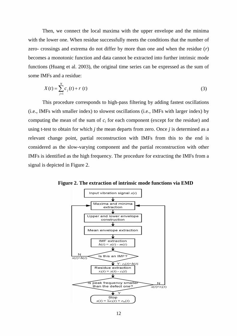
Then, we connect the local maxima with the upper envelope and the minima

with the lower one. When residue successfully meets the conditions that the number of

zero- crossings and extrema do not differ by more than one and when the residue (r)

becomes a monotonic function and data cannot be extracted into further intrinsic mode

functions (Huang et al. 2003), the original time series can be expressed as the sum of

some IMFs and a residue:

)()()(1

trtctXN

j

j

(3)

This procedure corresponds to high-pass filtering by adding fastest oscillations

(i.e., IMFs with smaller index) to slowest oscillations (i.e., IMFs with larger index) by

computing the mean of the sum of ci for each component (except for the residue) and

using t-test to obtain for which j the mean departs from zero. Once j is determined as a

relevant change point, partial reconstruction with IMFs from this to the end is

considered as the slow-varying component and the partial reconstruction with other

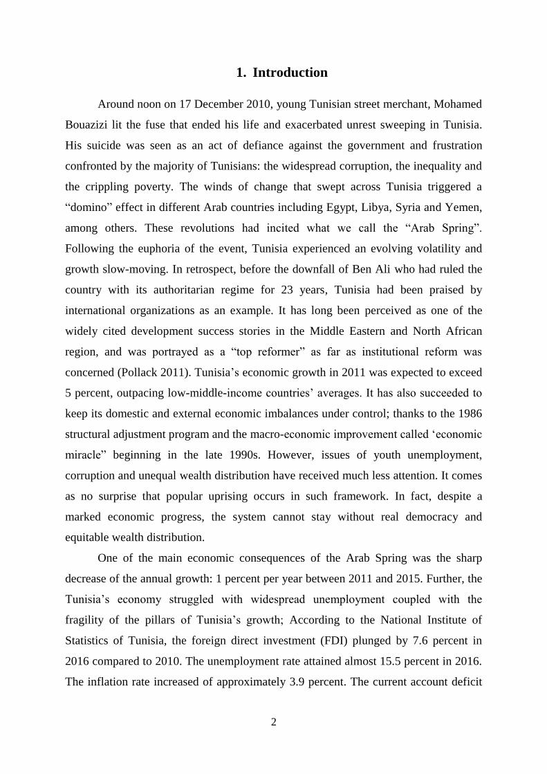
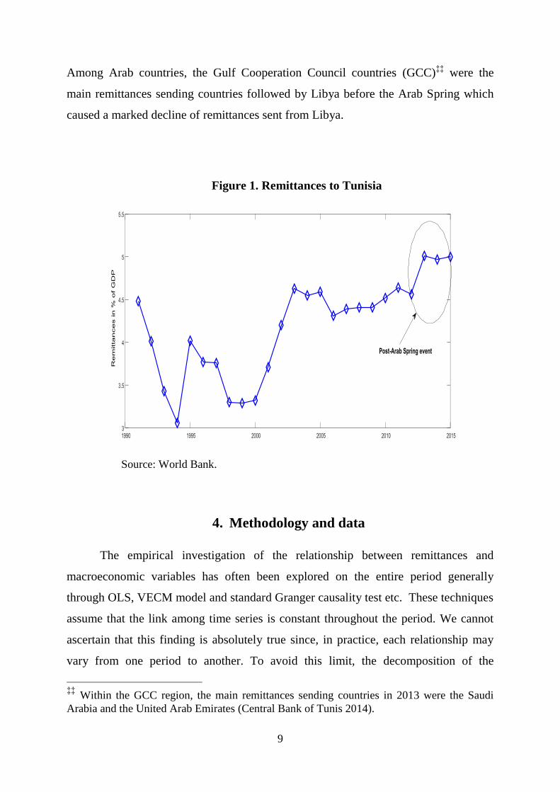
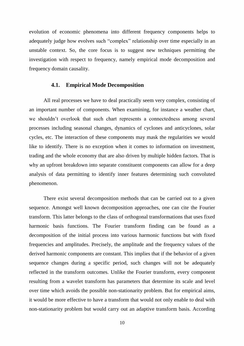
IMFs is identified as the high frequency. The procedure for extracting the IMFs from a

signal is depicted in Figure 2.

Figure 2. The extraction of intrinsic mode functions via EMD

13

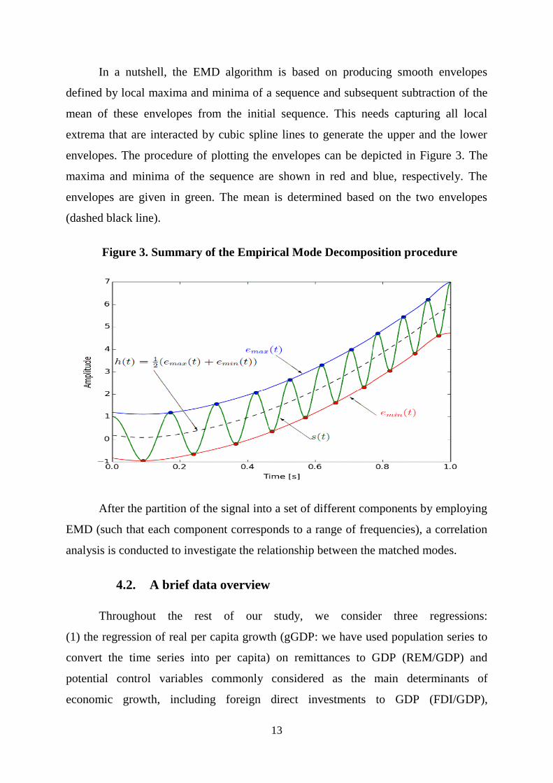
In a nutshell, the EMD algorithm is based on producing smooth envelopes

defined by local maxima and minima of a sequence and subsequent subtraction of the

mean of these envelopes from the initial sequence. This needs capturing all local

extrema that are interacted by cubic spline lines to generate the upper and the lower

envelopes. The procedure of plotting the envelopes can be depicted in Figure 3. The

maxima and minima of the sequence are shown in red and blue, respectively. The

envelopes are given in green. The mean is determined based on the two envelopes

(dashed black line).

Figure 3. Summary of the Empirical Mode Decomposition procedure

After the partition of the signal into a set of different components by employing

EMD (such that each component corresponds to a range of frequencies), a correlation

analysis is conducted to investigate the relationship between the matched modes.

4.2. A brief data overview

Throughout the rest of our study, we consider three regressions:

(1) the regression of real per capita growth (gGDP: we have used population series to

convert the time series into per capita) on remittances to GDP (REM/GDP) and

potential control variables commonly considered as the main determinants of

economic growth, including foreign direct investments to GDP (FDI/GDP),

14

investment to GDP (INV/GDP), credits to private sector (Credits/GDP), trade

openness (or the level of exports plus imports to GDP, noted OPEN), inflation (CPI)

and real effective exchange rate (REER: the ratio between prices of tradable and non-

tradable goods where an increase in price of tradable goods corresponds to a real

depreciation); (2) the regression of domestic investment (INV/GDP) on remittances

and further explanatory variables including (FDI/GDP), gGDP, Credits/GDP, OPEN,

CPI, and real interest rate (RIR); and (3) the regression of consumption to GDP

(CONS/GDP) on remittances, gGDP, Credits/GDP, CPI and RIR. Because we have

not enough observations to estimate after the Arab Spring, we have made two

estimates for two different periods: the first one corresponds to the period before the

Arab Spring spanning between 1990:Q1 and 2010:Q4 (i.e., 85 observations) and the

second one refers to an extended period (prior to and post Arab Spring event) that

spans between 1990:Q1 and 2015:Q3 (i.e., 104 observations).

The chosen sampling period is due to data availability. The data on remittances,

investment, real per capita growth and the additional explanatory variables **

were

collected from world development indicators (CD-ROM), quandl website and

EconstatsTM

. In order to assess the dynamic dependencies (correlation and causality)

among the focal variables, we have transformed the variables by taking natural

logarithms to correct for heteroskedasticity and dimensional differences between the

investigated time series.

5. Results

5.1. Results via standard techniques

We start our analysis by applying a VECM method for two periods: a restricted

period (i.e., before the aftermath of Arab Spring) and a whole period (before and after

the Arab Spring). This exercise aimed at having a case of benchmarking to compare

the VECM with a new econometric tool (i.e., correlation analysis-based EMD). To

proceed, we have, first, applied Ng-Perron (Ng-Perron 2001) unit root test to examine

whether the variables are stationary in the level or first difference form. Almost all the

**

Note that some potential control variables were not taken into account because of their

unavailability in quarterly frequency data.

15

variables under study showed unit root behavior at level and found stationary at 1st

difference with intercept and trend (Table A.1, Appendices). Due not having

information about structural breaks stemming in the time series, Ng-Perron unit root

findings may be biased. To solve this drawback, we use de-trended Zivot and Andrews

(1992)‟s structural break unit test to determine the integrating orders of the variables in

the presence of structural breaks. We note that, for the two periods investigated, all the

variables are stationary at specific levels showing structural breaks. Then, we employ a

VECM model in order to identify the channels through which the remittances may

promote economic growth in an unstable context. In particular, we regress remittances

on Tunisia‟s real economic growth, investment and consumption. The results are

reported, respectively, in Tables A.2, A.3 and A.4 (Appendices). We show that, for the

restricted period, there are negative and significant long-run relationships between (1)

remittances and growth, (2) remittances and investment, and (3) remittances and

consumption. These results change substantially when considering a lengthy period

(prior to and post Arab spring). Although remittances are still exerting a long-term

negative influence on investment, their effects on growth and consumption become

significantly positive but also on the long-run. These first estimations bring some

insights into the main channel through which remittances support economic growth

over uncertainty surrounding the economic prospects of Tunisia in the onset of Arab

Spring. The results of standard Granger causality test (Table A.5, Appendices) seem

consistent with those of VECM in terms of the extent of cycles between the variables

of interest. Although remittances flows Granger-cause INV/GDP for the two

concerned periods, they significantly caused gGDP and CONS/GDP in the whole

period. We will return later on the arguments explaining these results. But we must

clarify that these findings may be erroneous because they seek out information on

averages, and do not account for the problems of stationarity and nonlinearity.

The fundamental question of this study is beyond the classic debate which

opposes the remittances impact on consumption with that on investment. This research

analyzes whether these linkages evolve over different time-scales (or frequencies).

Also, it assesses to what extent does Arab Spring strengthen the remittance matters.

Our objective is to spotlight how decomposing the variables into intrinsic mode

16

functions can be useful in examining such relationships during turbulent times. Unlike

standard methods, signal approaches (in particular, a correlation analysis-based EMD

approach and a frequency domain causality test) permit to uncover the inner factors

that may drive the remittances‟ effects on growth, investment and consumption, which

would stay hidden otherwise.

5.2. EMD results

Figure A.1 (Appendices) displays the EMD outcomes for the variables of

interest. We show that, for the restricted and the whole period, the real per capita

growth, remittances, investment and consumption were decomposed into seven IMFs

plus one residue. Since the number of IMFs is limited and will be restricted to log2N

where N is the length of data****

, the sifting processes produced only seven IMFs for

each variable. All the derived IMFs were listed from high frequency component to low

frequency band, and the last one is the residue. Remarkably, the frequencies and

amplitudes of all the IMFs evolved over time and changed when moving from the first

period (before Arab Spring) to the second period (before and after Arab Spring). As

the frequency changes from high to low, the amplitudes of the IMFs become wider.

We discuss three main frequency components: short-run (IMF1 and IMF2), medium-

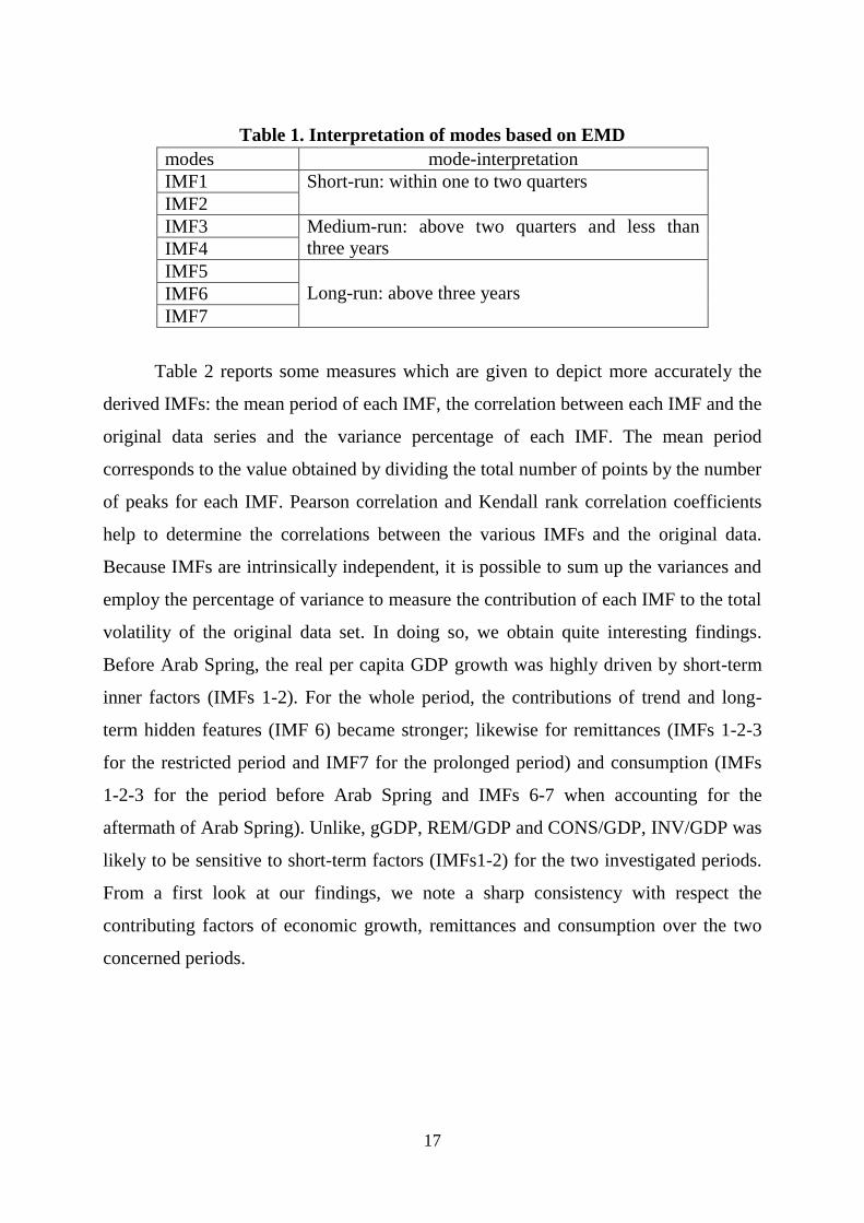
run (IMF3and IMF4) and long-run (IMF5, IMF6 and IMF7). Table 1 presents the time

scale interpretation of EMD. Since for the two considered periods, seven IMFs had

been derived, the interpretation of frequency components is the same for the two

investigated periods.

****

The EMD technique generates itself the modes depending to the data. For more details

about data extraction, please refer to Huang et al. (2003).

17

Table 1. Interpretation of modes based on EMD

modes mode-interpretation

IMF1 Short-run: within one to two quarters

IMF2

IMF3 Medium-run: above two quarters and less than

three years IMF4

IMF5

Long-run: above three years IMF6

IMF7

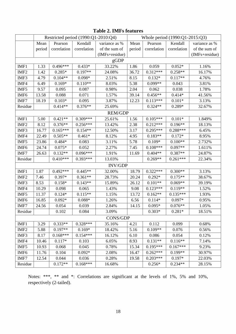
Table 2 reports some measures which are given to depict more accurately the

derived IMFs: the mean period of each IMF, the correlation between each IMF and the

original data series and the variance percentage of each IMF. The mean period

corresponds to the value obtained by dividing the total number of points by the number

of peaks for each IMF. Pearson correlation and Kendall rank correlation coefficients

help to determine the correlations between the various IMFs and the original data.

Because IMFs are intrinsically independent, it is possible to sum up the variances and

employ the percentage of variance to measure the contribution of each IMF to the total

volatility of the original data set. In doing so, we obtain quite interesting findings.

Before Arab Spring, the real per capita GDP growth was highly driven by short-term

inner factors (IMFs 1-2). For the whole period, the contributions of trend and long-

term hidden features (IMF 6) became stronger; likewise for remittances (IMFs 1-2-3

for the restricted period and IMF7 for the prolonged period) and consumption (IMFs

1-2-3 for the period before Arab Spring and IMFs 6-7 when accounting for the

aftermath of Arab Spring). Unlike, gGDP, REM/GDP and CONS/GDP, INV/GDP was

likely to be sensitive to short-term factors (IMFs1-2) for the two investigated periods.

From a first look at our findings, we note a sharp consistency with respect the

contributing factors of economic growth, remittances and consumption over the two

concerned periods.

18

Table 2. IMFs features

Restricted period (1990:Q1-2010:Q4) Whole period (1990:Q1-2015:Q3)

Mean

period

Pearson

correlation

Kendall

correlation

variance as %

of the sum of

(IMFs+residue)

Mean

period

Pearson

correlation

Kendall

correlation

variance as %

of the sum of

(IMFs+residue)

gGDP

IMF1 1.33 0.496*** 0.433* 33.22% 1.86 0.059 0.052* 1.16%

IMF2 1.42 0.285* 0.197** 24.08% 36.72 0.312*** 0.258** 16.17%

IMF3 4.79 0.104** 0.098* 2.51% 8.15 0.132* 0.117** 4.76%

IMF4 6.49 0.169* 0.110** 8.03% 5.38 0.099** 0.043 3.81%

IMF5 9.57 0.095 0.087 0.98% 2.04 0.062 0.038 1.78%

IMF6 13.58 0.088 0.071 1.57% 39.14 0.456** 0.414* 41.56%

IMF7 18.19 0.103* 0.095 3.87% 12.23 0.113*** 0.101* 3.13%

Residue 0.414** 0.376** 25.69% 0.324** 0.289* 32.67%

REM/GDP

IMF1 5.00 0.421** 0.309*** 25.61% 1.56 0.105*** 0.101* 1.849%

IMF2 8.12 0.376** 0.256*** 13.42% 2.38 0.212*** 0.196** 18.13%

IMF3 16.77 0.165*** 0.154** 12.50% 3.17 0.295*** 0.288*** 6.45%

IMF4 22.49 0.505** 0.461* 8.12% 4.95 0.183** 0.172* 8.95%

IMF5 23.86 0.484* 0.083 3.11% 5.78 0.109* 0.100** 2.732%

IMF6 24.74 0.075* 0.052 2.27% 7.45 0.108*** 0.097** 1.611%

IMF7 26.63 0.132** 0.096*** 1.91% 11.69 0.404** 0.387** 24.87%

Residue 0.410*** 0.393*** 13.03% 0.269** 0.261*** 22.34%

INV/GDP

IMF1 1.87 0.492*** 0.445** 32.00% 18.79 0.322*** 0.300** 3.13%

IMF2 7.46 0.397* 0.361** 28.73% 20.24 0.292* 0.175** 38.67%

IMF3 8.53 0.158* 0.143** 15.89% 26.12 0.101** 0.069** 39.19%

IMF4 10.29 0.098 0.065 1.43% 9.08 0.123*** 0.119** 1.52%

IMF5 11.37 0.124* 0.115** 1.15% 13.72 0.162** 0.135*** 1.93%

IMF6 16.85 0.092* 0.088* 1.26% 6.56 0.114* 0.097* 0.95%

IMF7 24.56 0.054 0.039 2.84% 14.15 0.095* 0.076** 1.05%

Residue 0.102 0.084 3.09% 0.303* 0.281* 18.51%

CONS/GDP

IMF1 3.29 0.333** 0.328*** 35.16% 4.21 0.112 0.099 0.68%

IMF2 5.88 0.197** 0.169* 18.42% 5.16 0.109** 0.076 0.56%

IMF3 8.17 0.168*** 0.154*** 16.12% 6.10 0.086 0.054 0.12%

IMF4 10.46 0.117* 0.103 6.05% 8.93 0.131** 0.116** 7.14%

IMF5 10.93 0.068 0.045 0.78% 15.34 0.195*** 0.167*** 9.23%

IMF6 11.76 0.104 0.092* 2.08% 16.47 0.262*** 0.199** 30.97%

IMF7 12.54 0.044 0.036 0.28% 19.58 0.203*** 0.197* 22.03%

Residue 0.172** 0.168*** 16.68% 0.256* 0.234** 28.15%

Notes: ***, ** and *: Correlations are significant at the levels of 1%, 5% and 10%,

respectively (2-tailed).

19

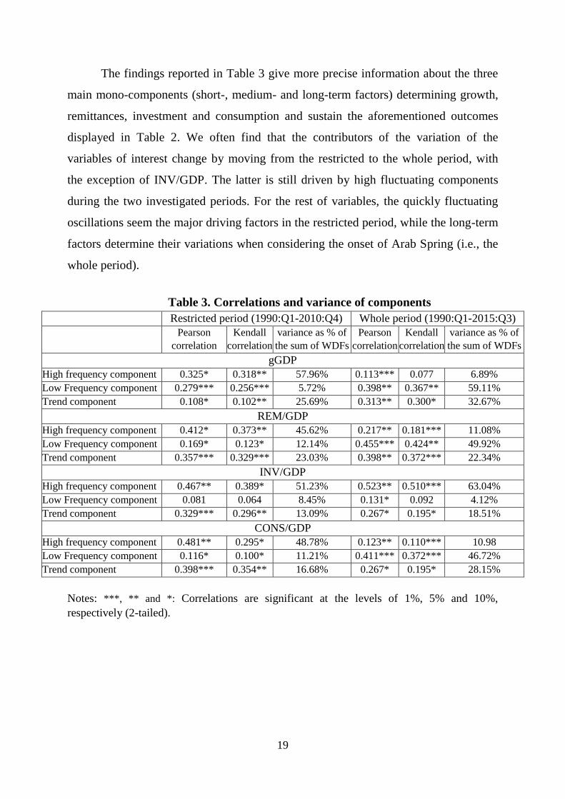
The findings reported in Table 3 give more precise information about the three

main mono-components (short-, medium- and long-term factors) determining growth,

remittances, investment and consumption and sustain the aforementioned outcomes

displayed in Table 2. We often find that the contributors of the variation of the

variables of interest change by moving from the restricted to the whole period, with

the exception of INV/GDP. The latter is still driven by high fluctuating components

during the two investigated periods. For the rest of variables, the quickly fluctuating

oscillations seem the major driving factors in the restricted period, while the long-term

factors determine their variations when considering the onset of Arab Spring (i.e., the

whole period).

Table 3. Correlations and variance of components

Restricted period (1990:Q1-2010:Q4) Whole period (1990:Q1-2015:Q3)

Pearson

correlation

Kendall

correlation

variance as % of

the sum of WDFs

Pearson

correlation

Kendall

correlation

variance as % of

the sum of WDFs

gGDP

High frequency component 0.325* 0.318** 57.96% 0.113*** 0.077 6.89%

Low Frequency component 0.279*** 0.256*** 5.72% 0.398** 0.367** 59.11%

Trend component 0.108* 0.102** 25.69% 0.313** 0.300* 32.67%

REM/GDP

High frequency component 0.412* 0.373** 45.62% 0.217** 0.181*** 11.08%

Low Frequency component 0.169* 0.123* 12.14% 0.455*** 0.424** 49.92%

Trend component 0.357*** 0.329*** 23.03% 0.398** 0.372*** 22.34%

INV/GDP

High frequency component 0.467** 0.389* 51.23% 0.523** 0.510*** 63.04%

Low Frequency component 0.081 0.064 8.45% 0.131* 0.092 4.12%

Trend component 0.329*** 0.296** 13.09% 0.267* 0.195* 18.51%

CONS/GDP

High frequency component 0.481** 0.295* 48.78% 0.123** 0.110*** 10.98

Low Frequency component 0.116* 0.100* 11.21% 0.411*** 0.372*** 46.72%

Trend component 0.398*** 0.354** 16.68% 0.267* 0.195* 28.15%

Notes: ***, ** and *: Correlations are significant at the levels of 1%, 5% and 10%,

respectively (2-tailed).

20

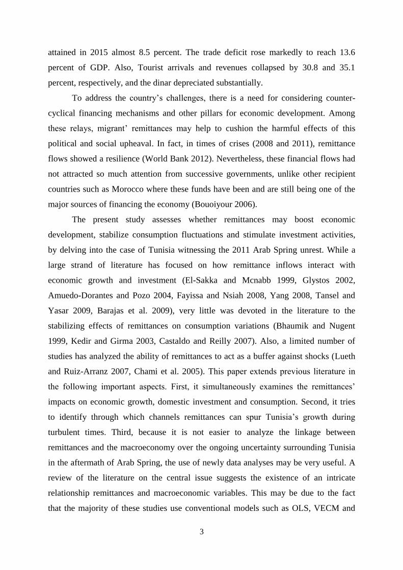
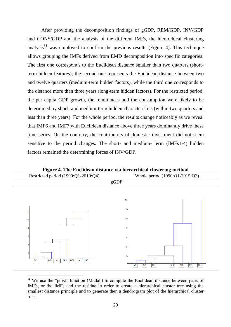
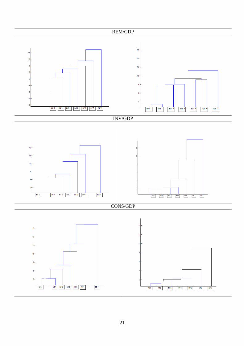
After providing the decomposition findings of gGDP, REM/GDP, INV/GDP

and CONS/GDP and the analysis of the different IMFs, the hierarchical clustering

analysis§§

was employed to confirm the previous results (Figure 4). This technique

allows grouping the IMFs derived from EMD decomposition into specific categories:

The first one corresponds to the Euclidean distance smaller than two quarters (short-

term hidden features); the second one represents the Euclidean distance between two

and twelve quarters (medium-term hidden factors), while the third one corresponds to

the distance more than three years (long-term hidden factors). For the restricted period,

the per capita GDP growth, the remittances and the consumption were likely to be

determined by short- and medium-term hidden characteristics (within two quarters and

less than three years). For the whole period, the results change noticeably as we reveal

that IMF6 and IMF7 with Euclidean distance above three years dominantly drive these

time series. On the contrary, the contributors of domestic investment did not seem

sensitive to the period changes. The short- and medium- term (IMFs1-4) hidden

factors remained the determining forces of INV/GDP.

Figure 4. The Euclidean distance via hierarchical clustering method

Restricted period (1990:Q1-2010:Q4) Whole period (1990:Q1-2015:Q3)

gGDP

§§

We use the “pdist” function (Matlab) to compute the Euclidean distance between pairs of

IMFs, or the IMFs and the residue in order to create a hierarchical cluster tree using the

smallest distance principle and to generate then a dendrogram plot of the hierarchical cluster

tree.

21

REM/GDP

INV/GDP

CONS/GDP

22

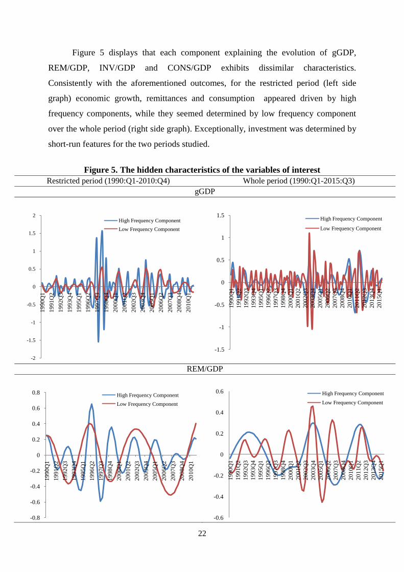
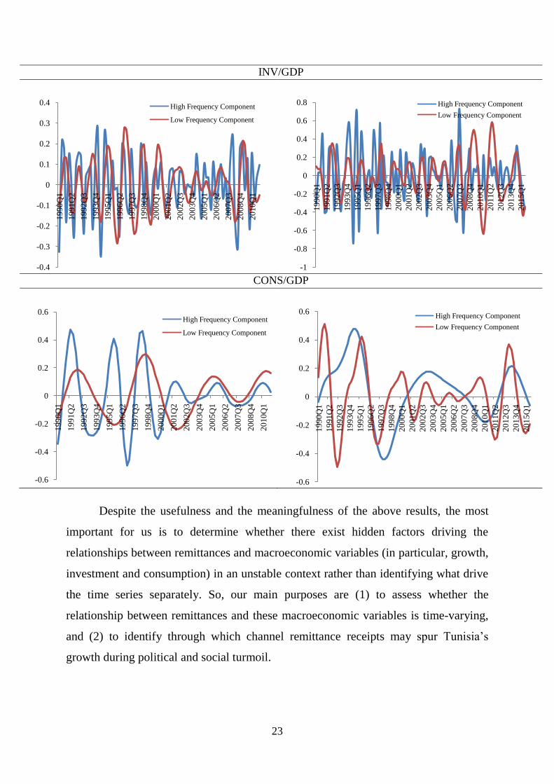
Figure 5 displays that each component explaining the evolution of gGDP,

REM/GDP, INV/GDP and CONS/GDP exhibits dissimilar characteristics.

Consistently with the aforementioned outcomes, for the restricted period (left side

graph) economic growth, remittances and consumption appeared driven by high

frequency components, while they seemed determined by low frequency component

over the whole period (right side graph). Exceptionally, investment was determined by

short-run features for the two periods studied.

Figure 5. The hidden characteristics of the variables of interest

Restricted period (1990:Q1-2010:Q4) Whole period (1990:Q1-2015:Q3)

gGDP

REM/GDP

-2

-1.5

-1

-0.5

0

0.5

1

1.5

2

19

90

Q1

19

91

Q2

19

92

Q3

19

93

Q4

19

95

Q1

19

96

Q2

19

97

Q3

19

98

Q4

20

00

Q1

20

01

Q2

20

02

Q3

20

03

Q4

20

05

Q1

20

06

Q2

20

07

Q3

20

08

Q4

20

10

Q1

High Frequency Component

Low Frequency Component

-1.5

-1

-0.5

0

0.5

1

1.5

19

90

Q1

19

91

Q2

19

92

Q3

19

93

Q4

19

95

Q1

19

96

Q2

19

97

Q3

19

98

Q4

20

00

Q1

20

01

Q2

20

02

Q3

20

03

Q4

20

05

Q1

20

06

Q2

20

07

Q3

20

08

Q4

20

10

Q1

20

11

Q2

20

12

Q3

20

13

Q4

20

15

Q1

High Frequency Component

Low Frequency Component

-0.8

-0.6

-0.4

-0.2

0

0.2

0.4

0.6

0.8

19

90

Q1

19

91

Q2

19

92

Q3

19

93

Q4

19

95

Q1

19

96

Q2

19

97

Q3

19

98

Q4

20

00

Q1

20

01

Q2

20

02

Q3

20

03

Q4

20

05

Q1

20

06

Q2

20

07

Q3

20

08

Q4

20

10

Q1

High Frequency Component

Low Frequency Component

-0.6

-0.4

-0.2

0

0.2

0.4

0.6

19

90

Q1

19

91

Q2

19

92

Q3

19

93

Q4

19

95

Q1

19

96

Q2

19

97

Q3

19

98

Q4

20

00

Q1

20

01

Q2

20

02

Q3

20

03

Q4

20

05

Q1

20

06

Q2

20

07

Q3

20

08

Q4

20

10

Q1

20

11

Q2

20

12

Q3

20

13

Q4

20

15

Q1

High Frequency Component

Low Frequency Component

23

INV/GDP

CONS/GDP

Despite the usefulness and the meaningfulness of the above results, the most

important for us is to determine whether there exist hidden factors driving the

relationships between remittances and macroeconomic variables (in particular, growth,

investment and consumption) in an unstable context rather than identifying what drive

the time series separately. So, our main purposes are (1) to assess whether the

relationship between remittances and these macroeconomic variables is time-varying,

and (2) to identify through which channel remittance receipts may spur Tunisia‟s

growth during political and social turmoil.

-0.4

-0.3

-0.2

-0.1

0

0.1

0.2

0.3

0.4

19

90

Q1

19

91

Q2

19

92

Q3

19

93

Q4

19

95

Q1

19

96

Q2

19

97

Q3

19

98

Q4

20

00

Q1

20

01

Q2

20

02

Q3

20

03

Q4

20

05

Q1

20

06

Q2

20

07

Q3

20

08

Q4

20

10

Q1

High Frequency Component

Low Frequency Component

-1

-0.8

-0.6

-0.4

-0.2

0

0.2

0.4

0.6

0.8

19

90

Q1

19

91

Q2

19

92

Q3

19

93

Q4

19

95

Q1

19

96

Q2

19

97

Q3

19

98

Q4

20

00

Q1

20

01

Q2

20

02

Q3

20

03

Q4

20

05

Q1

20

06

Q2

20

07

Q3

20

08

Q4

20

10

Q1

20

11

Q2

20

12

Q3

20

13

Q4

20

15

Q1

High Frequency Component

Low Frequency Component

-0.6

-0.4

-0.2

0

0.2

0.4

0.6

19

90

Q1

19

91

Q2

19

92

Q3

19

93

Q4

19

95

Q1

19

96

Q2

19

97

Q3

19

98

Q4

20

00

Q1

20

01

Q2

20

02

Q3

20

03

Q4

20

05

Q1

20

06

Q2

20

07

Q3

20

08

Q4

20

10

Q1

High Frequency Component

Low Frequency Component

-0.6

-0.4

-0.2

0

0.2

0.4

0.61

99

0Q

1

19

91

Q2

19

92

Q3

19

93

Q4

19

95

Q1

19

96

Q2

19

97

Q3

19

98

Q4

20

00

Q1

20

01

Q2

20

02

Q3

20

03

Q4

20

05

Q1

20

06

Q2

20

07

Q3

20

08

Q4

20

10

Q1

20

11

Q2

20

12

Q3

20

13

Q4

20

15

Q1

High Frequency Component

Low Frequency Component

24

5.3. A correlation analysis-based EMD

We use an OLS-based EMD to assess the dynamic dependencies among

remittances flows and macroeconomic variables in unstable context. Our procedure

consists of regressing remittances on gGDP, INV/GDP and CONS/GDP), even if we

account for potential control variables.

5.3.1. Remittances and growth

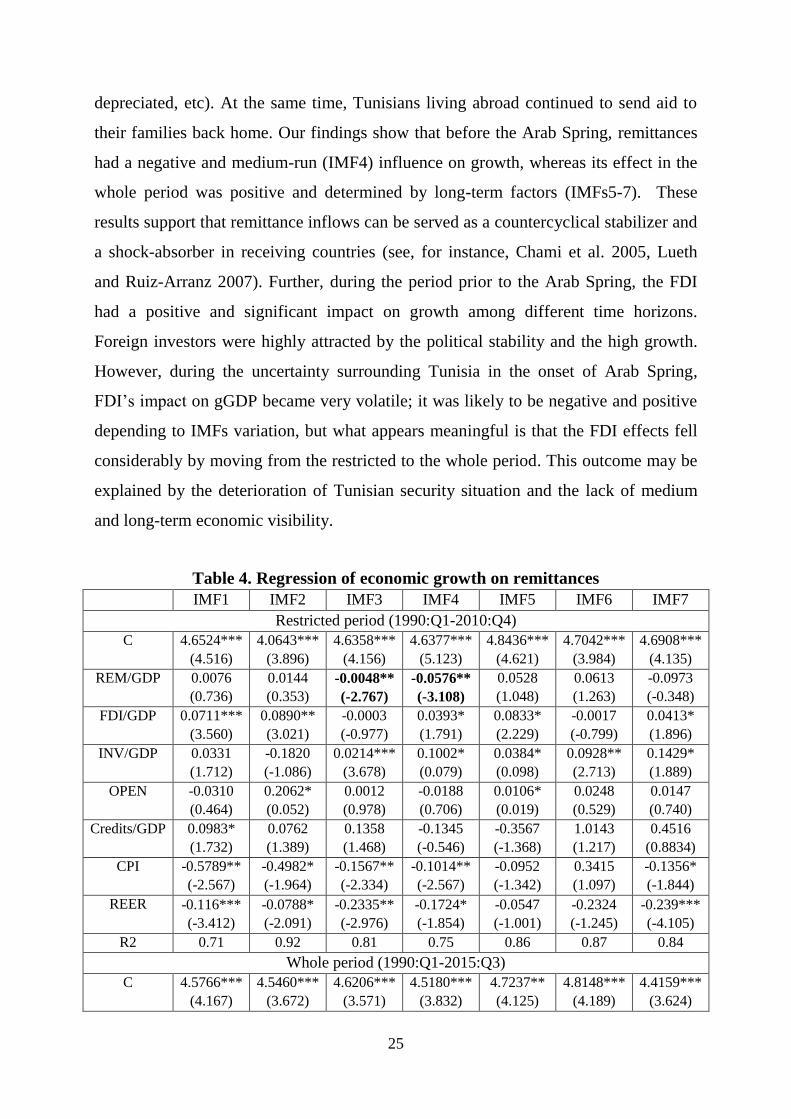
Table 4 summarizes the estimates related to the relationship between

remittances and economic growth. For the restricted period (i.e. before the onset of

“Arab Spring”), the relationship was negative, weak and occurred in the medium-run

(IMFs3-4). However, for the whole period (before and after the Arab Spring),

remittances exerted a positive and significant impact on Tunisia‟s growth; such

relationship was dominantly driven by long-term hidden factors (IMFs 5-7). It is true

that remittance flows have never been considered as a strategic variable in the

Tunisian economic policy. When comparing Tunisia to Morocco, the strategic path

towards migration and remittances seems totally opposed. Unlike Tunisia, Morocco

conducted an “aggressive” policy aimed at attracting remittances via the establishment

of organizations dedicated to migration (such as Ministry in Charge of Moroccans

living abroad, founding Council for the Moroccan Communities abroad, etc.). Add to

this that the economic situation of both countries is radically different. Before the Arab

Spring, Tunisia witnessed a stable economic and political conditions and strong

growth. Foreign investors tended to settle easily. The openness policy has played a

vital role in boosting the development of a solid and innovative manufacturing

industry. This is why, Tunisia was the “champion” compared to the rest of the MENA

region and a “good student” according to World Bank and IMF criteria. However, this

opulence masked a reality of corruption and inequality. Morocco was characterized by

a stable political situation, a great resilience in dealing with external shocks (2008

economic crisis and Arab Spring), but its growth is volatile due to its great dependency

on the whims of the sky. In the onset of Arab Spring, Tunisia‟s growth was

constrained, since its pillars weakened (i.e., the FDI and tourism collapsed, the dinar

25

depreciated, etc). At the same time, Tunisians living abroad continued to send aid to

their families back home. Our findings show that before the Arab Spring, remittances

had a negative and medium-run (IMF4) influence on growth, whereas its effect in the

whole period was positive and determined by long-term factors (IMFs5-7). These

results support that remittance inflows can be served as a countercyclical stabilizer and

a shock-absorber in receiving countries (see, for instance, Chami et al. 2005, Lueth

and Ruiz-Arranz 2007). Further, during the period prior to the Arab Spring, the FDI

had a positive and significant impact on growth among different time horizons.

Foreign investors were highly attracted by the political stability and the high growth.

However, during the uncertainty surrounding Tunisia in the onset of Arab Spring,

FDI‟s impact on gGDP became very volatile; it was likely to be negative and positive

depending to IMFs variation, but what appears meaningful is that the FDI effects fell

considerably by moving from the restricted to the whole period. This outcome may be

explained by the deterioration of Tunisian security situation and the lack of medium

and long-term economic visibility.

Table 4. Regression of economic growth on remittances

IMF1 IMF2 IMF3 IMF4 IMF5 IMF6 IMF7

Restricted period (1990:Q1-2010:Q4)

C 4.6524***

(4.516) 4.0643***

(3.896)

4.6358***

(4.156)

4.6377***

(5.123)

4.8436***

(4.621)

4.7042***

(3.984)

4.6908***

(4.135)

REM/GDP 0.0076

(0.736)

0.0144

(0.353)

-0.0048**

(-2.767)

-0.0576**

(-3.108)

0.0528

(1.048)

0.0613

(1.263)

-0.0973

(-0.348)

FDI/GDP 0.0711***

(3.560)

0.0890**

(3.021)

-0.0003

(-0.977)

0.0393*

(1.791)

0.0833*

(2.229)

-0.0017

(-0.799)

0.0413*

(1.896)

INV/GDP 0.0331

(1.712)

-0.1820

(-1.086)

0.0214***

(3.678)

0.1002*

(0.079)

0.0384*

(0.098)

0.0928**

(2.713)

0.1429*

(1.889)

OPEN -0.0310

(0.464)

0.2062*

(0.052)

0.0012

(0.978)

-0.0188

(0.706)

0.0106*

(0.019)

0.0248

(0.529)

0.0147

(0.740)

Credits/GDP 0.0983*

(1.732)

0.0762

(1.389)

0.1358

(1.468)

-0.1345

(-0.546)

-0.3567

(-1.368)

1.0143

(1.217)

0.4516

(0.8834)

CPI -0.5789**

(-2.567)

-0.4982*

(-1.964)

-0.1567**

(-2.334)

-0.1014**

(-2.567)

-0.0952

(-1.342)

0.3415

(1.097)

-0.1356*

(-1.844)

REER -0.116***

(-3.412)

-0.0788*

(-2.091)

-0.2335**

(-2.976)

-0.1724*

(-1.854)

-0.0547

(-1.001)

-0.2324

(-1.245)

-0.239***

(-4.105)

R2 0.71 0.92 0.81 0.75 0.86 0.87 0.84

Whole period (1990:Q1-2015:Q3)

C 4.5766***

(4.167)

4.5460***

(3.672)

4.6206***

(3.571)

4.5180***

(3.832)

4.7237**

(4.125)

4.8148***

(4.189)

4.4159***

(3.624)

26

REM/GDP 0.0091

(1.485)

0.0118

(1.374)

0.01206

(1.401)

-0.0233

(-0.164)

0.0792***

(3.452)

0.0933*

(1.976)

0.1192**

(2.567)

FDI/GDP 0.0813*

(1.864)

-0.0440

(-0.635)

0.0517

(1.092)

0.0138

(1.894)

0.0157

(0.297)

0.0156**

(2.761)

0.0862*

(1.987)

INV/GDP 0.0102

(1.342)

-0.0119

(-1.259)

0.0060

(0.727)

0.0683*

(1.903)

0.0197

(1.381)

0.0559*

(1.768)

0.0831***

(3.567)

OPEN 0.0467**

(2.199)

0.0678*

(1.893)

0.0923**

(2.765)

0.1013**

(2.436)

0.1109*

(1.876)

0.1098***

(3.157)

0.0965**

(2.345)

Credits/GDP 0.0876**

(1.976)

0.0652*

(1.874)

0.0908**

(2.694)

0.0563*

(1.876)

0.0197***

(5.139)

0.0352

(1.251)

0.0287***

(3.818)

CPI 0.0256

(1.234)

-0.0324

(-0.528)

-0.1143*

(-1.785)

-0.0769*

(-1.863)

-0.0119

(-0.693)

-0.0386*

(-1.789)

-0.0837

(0.217)

REER -0.2522*

(-1.897)

-0.3242*

(-1.692)

-0.229***

(-3.456)

-0.160***

(-3.145)

-0.0686*

(-1.945)

-0.0251*

(-2.118)

-0.0264**

(-2.651)

R2 0.82 0.82 0.82 0.73 0.80 0.90 0.78

Notes: ***, ** and * imply significance at the 1%, 5% and 10%, respectively.

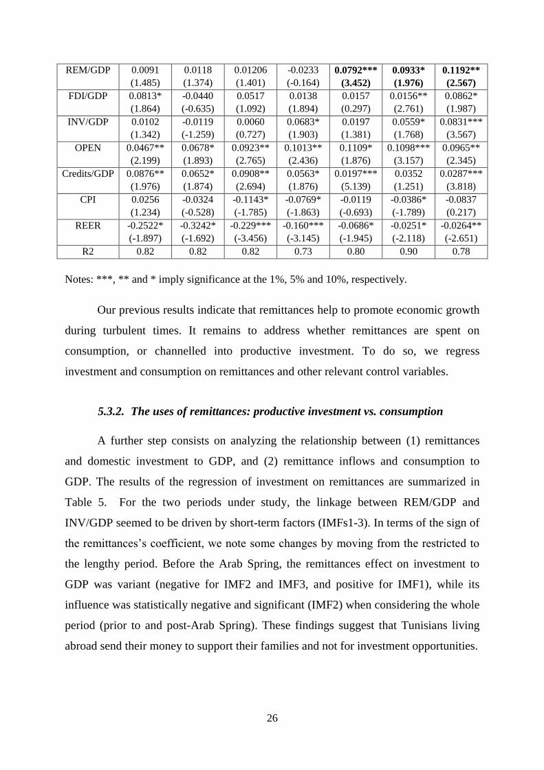
Our previous results indicate that remittances help to promote economic growth

during turbulent times. It remains to address whether remittances are spent on

consumption, or channelled into productive investment. To do so, we regress

investment and consumption on remittances and other relevant control variables.

5.3.2. The uses of remittances: productive investment vs. consumption

A further step consists on analyzing the relationship between (1) remittances

and domestic investment to GDP, and (2) remittance inflows and consumption to

GDP. The results of the regression of investment on remittances are summarized in

Table 5. For the two periods under study, the linkage between REM/GDP and

INV/GDP seemed to be driven by short-term factors (IMFs1-3). In terms of the sign of

the remittances‟s coefficient, we note some changes by moving from the restricted to

the lengthy period. Before the Arab Spring, the remittances effect on investment to

GDP was variant (negative for IMF2 and IMF3, and positive for IMF1), while its

influence was statistically negative and significant (IMF2) when considering the whole

period (prior to and post-Arab Spring). These findings suggest that Tunisians living

abroad send their money to support their families and not for investment opportunities.

27

Table 5. Regression of investment on remittances

IMF1 IMF2 IMF3 IMF4 IMF5 IMF6 IMF7

Restricted period (1990:Q1-2010:Q4)

C 1.9203

(1.122)

1.3803

(1.327)

1.8219

(1.266)

2.0042

(1.523)

3.6555***

(3.254)

4.3255***

(3.645)

1.8023**

(2.895)

REM/GDP 0.0763*

(1.812)

-0.0807*

(-1.942)

-0.0621*

(-1.734)

0.0187

(0.121)

0.0210

(0.112)

0.0200

(1.161)

0.5723

(0.408)

FDI/GDP 0.0353

(0.597)

-0.0550*

(-1.841)

-0.0759*

(-1.871)

0.0138

(0.440)

0.0833

(0.654)

-0.016***

(-3.176)

-0.0275**

(-2.358)

gGDP 0.0134

(0.703)

-0.0106

(0.801)

-0.0073

(0.870)

0.0093

(0.553)

-0.0201

(0.736)

0.0183

(1.297)

0.0363*

(1.761)

OPEN 0.0932

(1.213)

0.0763**

(2.451)

0.0764*

(1.893)

0.4321

(1.279)

0.0679*

(1.843)

0.1389

(1.267)

0.1056**

(2.418)

Credits/GDP 0.3167

(1.512)

0.1982

(1.367)

0.0113*

(1.768)

0.0345**

(2.456)

0.0452**

(2.138)

0.0512*

(1.913)

0.1567

(1.083)

CPI -0.1698**

(0.002)

-0.1690**

(0.005)

-0.1777**

(0.007)

-0.1118*

(0.030)

0.1393*

(0.076)

0.0048

(0.873)

-0.0194

(0.512)

RIR -0.211***

(0.000)

-0.222***

(0.000)

-0.220***

(0.000)

-0.217***

(0.000)

-0.195***

(0.000)

-0.061***

(0.000)

-0.059***

(0.000)

R2 0.89 0.87 0.84 0.80 0.75 0.92 0.95

Whole period (1990:Q1-2015:Q3)

C 7.5233***

(3.562)

7.6826**

(2.675)

8.3058*

(1.672)

8.6777***

(3.845)

8.6513***

(3.345)

1.5678

(1.004)

7.5233*

(1.976)

REM/GDP -0.452

(-1.328)

-0.123**

(-2.514)

0.2816

(0.252)

-0.1377

(-0.839)

0.0184

(1.037)

-0.0070

(-0.982)

0.2815

(0.276)

FDI/GDP 0.0165

(0.015)

-0.0321*

(-1.834)

0.0432*

(-1.697)

-0.0020

(-0.730)

-0.0125

(-0.170)

-0.0106

(-0.318)

-0.0165*

(-2.132)

gGDP 0.0421

(0.275)

-0.0120

(0.192)

0.0096

(0.184)

0.0074

(0.372)

0.0881**

(2.545)

0.0686***

(2.632)

0.1345

(1.307)

OPEN 0.1084*

(1.884)

0.0452***

(3.551)

0.0333***

(4.162)

0.0371***

(3.742)

0.1097*

(1.941)

0.0817*

(1.876)

0.1084

(1.221)

Credits/GDP 0.0568*

(1.899)

0.4135

(0.522)

0.0755*

(2.066)

-0.0658

(-0.920)

-0.0612

(-0.931)

0.0157**

(3.008)

0.1414

(0.752)

CPI -0.0216*

(-2.093)

0.0258

(0.273)

-0.0130

(-0.528)

-0.0030

(0.898)

-0.0251*

(-1.876)

0.0194

(0.532)

-0.0216

(-1.133)

RIR -0.0121*

(-1.698)

-0.0370

(-0.213)

-0.0183*

(-2.083)

-0.0023

(-0.934)

-0.0070

(-0.807)

-0.1223*

(-1.765)

-0.0121*

(-1.945)

R2 0.95 0.94 0.96 0.95 0.91 0.85 0.95

Notes: ***, ** and * imply significance at the 1%, 5% and 10%, respectively.

Table 6 reports the outcomes of the regression of consumption on remittance

inflows. For the period prior to the aftermath of Arab Spring, a positive link between

the focal variables was found in short-run (IMFs1-2). However, by considering the

post Arab Spring period, we show that the impact of remittances on consumption

became positive and more pronounced (i.e., driven by long-term inner features:

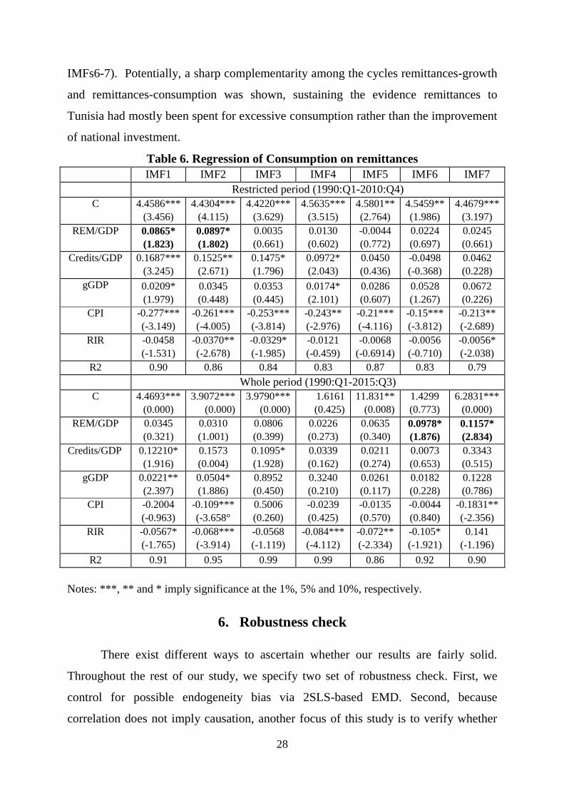
28

IMFs6-7). Potentially, a sharp complementarity among the cycles remittances-growth

and remittances-consumption was shown, sustaining the evidence remittances to

Tunisia had mostly been spent for excessive consumption rather than the improvement

of national investment.

Table 6. Regression of Consumption on remittances

IMF1 IMF2 IMF3 IMF4 IMF5 IMF6 IMF7

Restricted period (1990:Q1-2010:Q4)

C 4.4586***

(3.456)

4.4304***

(4.115)

4.4220***

(3.629)

4.5635***

(3.515)

4.5801**

(2.764)

4.5459**

(1.986)

4.4679***

(3.197)

REM/GDP 0.0865*

(1.823)

0.0897*

(1.802)

0.0035

(0.661)

0.0130

(0.602)

-0.0044

(0.772)

0.0224

(0.697)

0.0245

(0.661)

Credits/GDP 0.1687***

(3.245)

0.1525**

(2.671)

0.1475*

(1.796)

0.0972*

(2.043)

0.0450

(0.436)

-0.0498

(-0.368)

0.0462

(0.228)

gGDP

0.0209*

(1.979)

0.0345

(0.448)

0.0353

(0.445)

0.0174*

(2.101)

0.0286

(0.607)

0.0528

(1.267)

0.0672

(0.226)

CPI -0.277***

(-3.149)

-0.261***

(-4.005)

-0.253***

(-3.814)

-0.243**

(-2.976)

-0.21***

(-4.116)

-0.15***

(-3.812)

-0.213**

(-2.689)

RIR -0.0458

(-1.531)

-0.0370**

(-2.678)

-0.0329*

(-1.985)

-0.0121

(-0.459)

-0.0068

(-0.6914)

-0.0056

(-0.710)

-0.0056*

(-2.038)

R2 0.90 0.86 0.84 0.83 0.87 0.83 0.79

Whole period (1990:Q1-2015:Q3)

C 4.4693***

(0.000)

3.9072***

(0.000)

3.9790***

(0.000)

1.6161

(0.425)

11.831**

(0.008)

1.4299

(0.773)

6.2831***

(0.000)

REM/GDP 0.0345

(0.321)

0.0310

(1.001)

0.0806

(0.399)

0.0226

(0.273)

0.0635

(0.340)

0.0978*

(1.876)

0.1157*

(2.834)

Credits/GDP 0.12210*

(1.916)

0.1573

(0.004)

0.1095*

(1.928)

0.0339

(0.162)

0.0211

(0.274)

0.0073

(0.653)

0.3343

(0.515)

gGDP 0.0221**

(2.397)

0.0504*

(1.886)

0.8952

(0.450)

0.3240

(0.210)

0.0261

(0.117)

0.0182

(0.228)

0.1228

(0.786)

CPI -0.2004

(-0.963)

-0.109***

(-3.658°

0.5006

(0.260)

-0.0239

(0.425)

-0.0135

(0.570)

-0.0044

(0.840)

-0.1831**

(-2.356)

RIR

-0.0567*

(-1.765)

-0.068***

(-3.914)

-0.0568

(-1.119)

-0.084***

(-4.112)

-0.072**

(-2.334)

-0.105*

(-1.921)

0.141

(-1.196)

R2 0.91 0.95 0.99 0.99 0.86 0.92 0.90

Notes: ***, ** and * imply significance at the 1%, 5% and 10%, respectively.

6. Robustness check

There exist different ways to ascertain whether our results are fairly solid.

Throughout the rest of our study, we specify two set of robustness check. First, we

control for possible endogeneity bias via 2SLS-based EMD. Second, because

correlation does not imply causation, another focus of this study is to verify whether

29

there exists a frequency-by-frequency causal relation between remittances and the

central macroeconomic variables (growth, investment and consumption).

To this end, we utilize a frequency domain causality test

While EMD is performed within a discrete time framework, the frequency domain

causality has a spectral content across a continuous range ‡‡‡‡

.

6.1. Endogeneity

The endogeneity bias is one of the methodological challenges that confront

research on international migration and remittances. This can occur if remittances are

sent to home country for altruistic motives or if there is an increase in workers‟

remittances coincided with a rise in migration from countries with low economic

growth. A way to correct for the endogeneity biases is to carry out two-stage least

squares (2SLS) or GMM using lag of the explanatory variables as instruments (see, for

example, Giuliano and Ruiz-Arranz 2009 and Barajas et al. 2009). In the current study,

we apply a 2SLS-based EMD to re-analyze the dynamic dependency between

remittances inflows and macroeconomy in an unstable context, while controlling for

endogeneity problem. We summarize the 2SLS-based EMD findings of the regressions

of growth, investment and consumption on remittances and further explanatory

variables in Tables 7, 8 and 9, respectively.

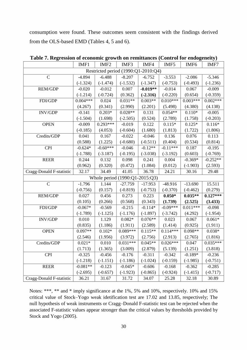
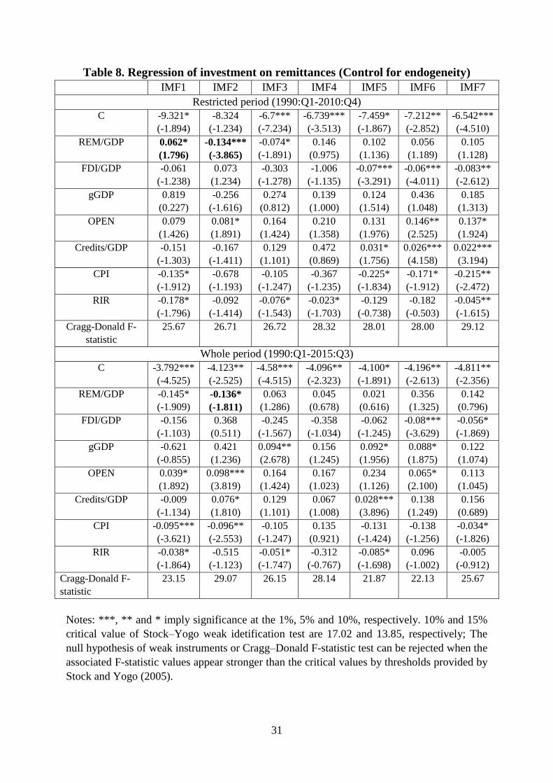
Our results robustly reveal that before the onset of Arab Spring, remittances

affected negatively the per capita economic growth and positively the consumption;

such relationships held in the short- or the medium-run. However, we note a time-

varying impact of these financial flows on domestic investment; it was negative in

some IMFs (IMF2) and positive in others (IMF1), but it was likely to be significant

only in the short-term. By accounting for the post-Arab Spring period, the investment

effect of remittance inflows became weaker and determined by short- and medium-

term factors, while a positive, strong and long-run remittances‟ effects on growth and

‡‡‡‡

The frequency domain causality test provides clearer cycle information almost in real

time, while business cycles cannot be identified before a cycle has been completed.

30

consumption were found. These outcomes seem consistent with the findings derived

from the OLS-based EMD (Tables 4, 5 and 6).

Table 7. Regression of economic growth on remittances (Control for endogeneity)

IMF1 IMF2 IMF3 IMF4 IMF5 IMF6 IMF7

Restricted period (1990:Q1-2010:Q4)

C -4.894

(-1.324)

-6.488

(-1.474)

-8.207

(-1.532)

-6.752

(-1.347)

-3.553

(-0.753)

-2.086

(-0.493)

-5.346

(-1.236)

REM/GDP -0.020

(-1.214)

-0.012

(-0.724)

0.007

(0.362)

-0.019**

(-2.316)

-0.014

(-0.220)

0.067

(0.654)

-0.009

(-0.359)

FDI/GDP 0.004***

(4.267)

0.024

(0.341)

0.031**

(2.990)

0.003**

(2.201)

0.010***

(5.498)

0.003***

(4.380)

0.002***

(4.138)

INV/GDP -0.141

(-1.504)

0.203*

(1.698)

0.028**

(-2.505)

0.131

(0.524)

0.054**

(2.789)

0.110*

(1.758)

-0.005

(-0.203)

OPEN -0.009

(-0.185)

0.293***

(4.053)

-0.019

(-0.604)

0.122

(1.680)

0.115*

(1.813)

0.125*

(1.722)

0.116*

(1.806)

Credits/GDP 0.041

(0.588)

0.167

(1.225)

-0.022

(-0.680)

-0.046

(-0.511)

0.136

(0.404)

0.076

(0.534)

0.113

(0.814)

CPI -0.624*

(-1.788)

-0.60***

(-3.187)

-0.046

(-0.195)

-0.12**

(-3.038)

-0.11***

(-3.192)

0.187

(0.603)

-0.195

(-0.769)

REER 0.244

(0.962)

0.132

(0.320)

0.098

(0.472)

0.241

(1.084)

0.004

(0.012)

-0.369*

(-1.903)

-0.252**

(2.593)

Cragg-Donald F-statistic 32.17 34.49 41.05 36.78 24.21 30.16 29.48

Whole period (1990:Q1-2015:Q3)

C -1.796

(-0.756)

1.144

(0.157)

-27.759

(-0.819)

-17.953

(-0.753)

-48.916

(-0.370)

-13.690

(-0.462)

15.511

(0.279)

REM/GDP 0.027

(0.105)

0.456

(0.266)

0.273

(0.568)

0.223

(0.343)

0.050*

(1.739)

0.035**

(2.525)

0.127***

(3.433)

FDI/GDP -0.067*

(-1.789)

-0.569

(-1.125)

-0.215

(-1.176)

-0.114*

(-1.897)

-0.09***

(-3.742)

0.011***

(4.292)

-0.098

(-1.954)

INV/GDP 0.010

(0.835)

1.129

(1.186)

0.082*

(1.911)

0.076**

(2.589)

0.023

(1.414)

0.067

(0.925)

0.061*

(1.911)

OPEN 0.097**

(2.546)

0.102*

(1.956)

0.089***

(3.972)

0.115**

(2.756)

0.114***

(2.913)

0.098**

(2.765)

0.038*

(1.816)

Credits/GDP 0.021*

(1.713)

0.010

(1.365)

0.031***

(3.009)

0.045**

(2.879)

0.026***

(5.139)

0.047

(1.251)

0.035***

(3.818)

CPI -0.325

(-1.218)

-0.456

(-1.151)

-0.176

(-1.186)

-0.311

(-1.024)

-0.342

(-0.159)

-0.189*

(-1.985)

-0.236

(-0.751)

REER -0.081**

(-2.695)

-0.123

(-0.657)

-0.045*

(-1.923)

-0.606

(-0.865)

-0.168

(-0.924)

-0.362

(-1.415)

-0.285

(-0.717)

Cragg-Donald F-statistic 36.21 31.67 31.72 34.07 25.28 32.18 30.89

Notes: ***, ** and * imply significance at the 1%, 5% and 10%, respectively. 10% and 15%

critical value of Stock–Yogo weak idetification test are 17.02 and 13.85, respectively; The

null hypothesis of weak instruments or Cragg–Donald F-statistic test can be rejected when the

associated F-statistic values appear stronger than the critical values by thresholds provided by

Stock and Yogo (2005).

31

Table 8. Regression of investment on remittances (Control for endogeneity)

IMF1 IMF2 IMF3 IMF4 IMF5 IMF6 IMF7

Restricted period (1990:Q1-2010:Q4)

C -9.321*

(-1.894)

-8.324

(-1.234)

-6.7***

(-7.234)

-6.739***

(-3.513)

-7.459*

(-1.867)

-7.212**

(-2.852)

-6.542***

(-4.510)

REM/GDP 0.062*

(1.796)

-0.134***

(-3.865)

-0.074*

(-1.891)

0.146

(0.975)

0.102

(1.136)

0.056

(1.189)

0.105

(1.128)

FDI/GDP -0.061

(-1.238)

0.073

(1.234)

-0.303

(-1.278)

-1.006

(-1.135)

-0.07***

(-3.291)

-0.06***

(-4.011)

-0.083**

(-2.612)

gGDP 0.819

(0.227)

-0.256

(-1.616)

0.274

(0.812)

0.139

(1.000)

0.124

(1.514)

0.436

(1.048)

0.185

(1.313)

OPEN 0.079

(1.426)

0.081*

(1.891)

0.164

(1.424)

0.210

(1.358)

0.131

(1.976)

0.146**

(2.525)

0.137*

(1.924)

Credits/GDP -0.151

(-1.303)

-0.167

(-1.411)

0.129

(1.101)

0.472

(0.869)

0.031*

(1.756)

0.026***

(4.158)

0.022***

(3.194)

CPI -0.135*

(-1.912)

-0.678

(-1.193)

-0.105

(-1.247)

-0.367

(-1.235)

-0.225*

(-1.834)

-0.171*

(-1.912)

-0.215**

(-2.472)

RIR -0.178*

(-1.796)

-0.092

(-1.414)

-0.076*

(-1.543)

-0.023*

(-1.703)

-0.129

(-0.738)

-0.182

(-0.503)

-0.045**

(-1.615)

Cragg-Donald F-

statistic

25.67 26.71 26.72 28.32 28.01 28.00 29.12

Whole period (1990:Q1-2015:Q3)

C -3.792***

(-4.525)

-4.123**

(-2.525)

-4.58***

(-4.515)

-4.096**

(-2.323)

-4.100*

(-1.891)

-4.196**

(-2.613)

-4.811**

(-2.356)

REM/GDP -0.145*

(-1.909)

-0.136*

(-1.811)

0.063

(1.286)

0.045

(0.678)

0.021

(0.616)

0.356

(1.325)

0.142

(0.796)

FDI/GDP -0.156

(-1.103)

0.368

(0.511)

-0.245

(-1.567)

-0.358

(-1.034)

-0.062

(-1.245)

-0.08***

(-3.629)

-0.056*

(-1.869)

gGDP -0.621

(-0.855)

0.421

(1.236)

0.094**

(2.678)

0.156

(1.245)

0.092*

(1.956)

0.088*

(1.875)

0.122

(1.074)

OPEN 0.039*

(1.892)

0.098***

(3.819)

0.164

(1.424)

0.167

(1.023)

0.234

(1.126)

0.065*

(2.100)

0.113

(1.045)

Credits/GDP -0.009

(-1.134)

0.076*

(1.810)

0.129

(1.101)

0.067

(1.008)

0.028***

(3.896)

0.138

(1.249)

0.156

(0.689)

CPI -0.095***

(-3.621)

-0.096**

(-2.553)

-0.105

(-1.247)

0.135

(0.921)

-0.131

(-1.424)

-0.138

(-1.256)

-0.034*

(-1.826)

RIR -0.038*

(-1.864)

-0.515

(-1.123)

-0.051*

(-1.747)

-0.312

(-0.767)

-0.085*

(-1.698)

0.096

(-1.002)

-0.005

(-0.912)

Cragg-Donald F-

statistic

23.15 29.07 26.15 28.14 21.87 22.13 25.67

Notes: ***, ** and * imply significance at the 1%, 5% and 10%, respectively. 10% and 15%

critical value of Stock–Yogo weak idetification test are 17.02 and 13.85, respectively; The

null hypothesis of weak instruments or Cragg–Donald F-statistic test can be rejected when the

associated F-statistic values appear stronger than the critical values by thresholds provided by

Stock and Yogo (2005).

32

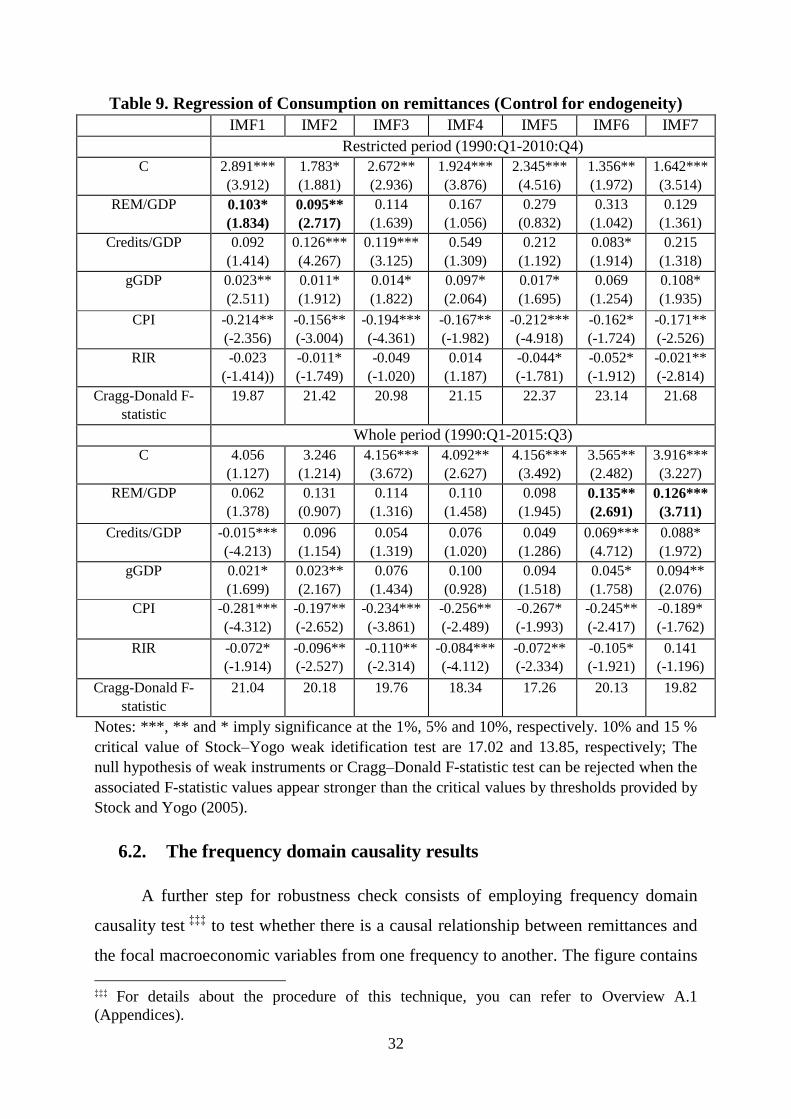
Table 9. Regression of Consumption on remittances (Control for endogeneity)

IMF1 IMF2 IMF3 IMF4 IMF5 IMF6 IMF7

Restricted period (1990:Q1-2010:Q4)

C 2.891***

(3.912)

1.783*

(1.881)

2.672**

(2.936)

1.924***

(3.876)

2.345***

(4.516)

1.356**

(1.972)

1.642***

(3.514)

REM/GDP 0.103*

(1.834)

0.095**

(2.717)

0.114

(1.639)

0.167

(1.056)

0.279

(0.832)

0.313

(1.042)

0.129

(1.361)

Credits/GDP 0.092

(1.414)

0.126***

(4.267)

0.119***

(3.125)

0.549

(1.309)

0.212

(1.192)

0.083*

(1.914)

0.215

(1.318)

gGDP

0.023**

(2.511)

0.011*

(1.912)

0.014*

(1.822)

0.097*

(2.064)

0.017*

(1.695)

0.069

(1.254)

0.108*

(1.935)

CPI -0.214**

(-2.356)

-0.156**

(-3.004)

-0.194***

(-4.361)

-0.167**

(-1.982)

-0.212***

(-4.918)

-0.162*

(-1.724)

-0.171**

(-2.526)

RIR -0.023

(-1.414))

-0.011*

(-1.749)

-0.049

(-1.020)

0.014

(1.187)

-0.044*

(-1.781)

-0.052*

(-1.912)

-0.021**

(-2.814)

Cragg-Donald F-

statistic

19.87 21.42 20.98 21.15 22.37 23.14 21.68

Whole period (1990:Q1-2015:Q3)

C 4.056

(1.127)

3.246

(1.214)

4.156***

(3.672)

4.092**

(2.627)

4.156***

(3.492)

3.565**

(2.482)

3.916***

(3.227)

REM/GDP

0.062

(1.378)

0.131

(0.907)

0.114

(1.316)

0.110

(1.458)

0.098

(1.945)

0.135**

(2.691)

0.126***

(3.711)

Credits/GDP -0.015***

(-4.213)

0.096

(1.154)

0.054

(1.319)

0.076

(1.020)

0.049

(1.286)

0.069***

(4.712)

0.088*

(1.972)

gGDP 0.021*

(1.699)

0.023**

(2.167)

0.076

(1.434)

0.100

(0.928)

0.094

(1.518)

0.045*

(1.758)

0.094**

(2.076)

CPI

-0.281***

(-4.312)

-0.197**

(-2.652)

-0.234***

(-3.861)

-0.256**

(-2.489)

-0.267*

(-1.993)

-0.245**

(-2.417)

-0.189*

(-1.762)

RIR

-0.072*

(-1.914)

-0.096**

(-2.527)

-0.110**

(-2.314)

-0.084***

(-4.112)

-0.072**

(-2.334)

-0.105*

(-1.921)

0.141

(-1.196)

Cragg-Donald F-

statistic

21.04 20.18 19.76 18.34 17.26 20.13 19.82

Notes: ***, ** and * imply significance at the 1%, 5% and 10%, respectively. 10% and 15 %

critical value of Stock–Yogo weak idetification test are 17.02 and 13.85, respectively; The

null hypothesis of weak instruments or Cragg–Donald F-statistic test can be rejected when the

associated F-statistic values appear stronger than the critical values by thresholds provided by

Stock and Yogo (2005).

6.2. The frequency domain causality results

A further step for robustness check consists of employing frequency domain

causality test ‡‡‡

to test whether there is a causal relationship between remittances and

the focal macroeconomic variables from one frequency to another. The figure contains

‡‡‡

For details about the procedure of this technique, you can refer to Overview A.1

(Appendices).

33

the test statistics with their 5 percent critical values for the frequency bands involved

(solid line) over the interval [0, π]. The frequency on the horizontal axis can be

translated into a cycle or periodicity of T weeks by where T is the period.

Figure 6.1 describes the evolution of the causal relationship between growth

and remittances depending to frequency transformations. Before the Arab Spring, we

support a medium-run unidirectional causality from remittances to growth, especially

when corresponding to a cycle length between 2.4 and 4.5 quarters.

However, a long-run causal relation running from remittances to growth happened

when focusing on the whole period (before and after the Arab Spring), in particular

when , corresponding to a cycle superior to 6.4 quarters. The reverse

link is not validated at any frequency and at any estimation period.

For the remittances impact on investment, a slight change was marked by

moving from the restricted to the whole period (Figure 6.2). Prior to Arab Spring

event, remittance inflows Granger-caused domestic investment in high frequencies

(when 03.381.2 , in particular for a cycle less than 2.2 quarters). This

relationship remained driven by quickly fluctuating components for the whole period.

Nevertheless, the remittances‟ impact on INV/GDP was stronger for the second period

as the cycle expands to 2.7 quarters ( 03.327.2 ). As the cycle remittances-

growth (Figure 6.1), a causal link running from remittances to consumption (Figure

6.3) was supported in the short-run for the restricted period (when 03.370.2 ),

corresponding to a cycle length inferior to 2.3 quarters) and in the long-run for the

whole period (when 54.001.0 ) corresponding to a cycle above 11.6 quarters).

Overall, the frequency domain causality findings seem consistent with the

correlation analysis-based EMD. Specifically, the consideration of the Arab spring

period in our estimates led to sharp changes in the cycles remittances-growth and

remittances- consumption; the cycles which were valid in the short term for the

restricted period, became explained by long-term oscillations for the whole period.

This confirms the consistency of these two cycles. The cycle remittances-investment

changed too but moderately; the linkage between REM/GDP and INV/GDP remained

driven by short-term factors for the two periods.

)(

)/2( T

60.230.1

98.001.0

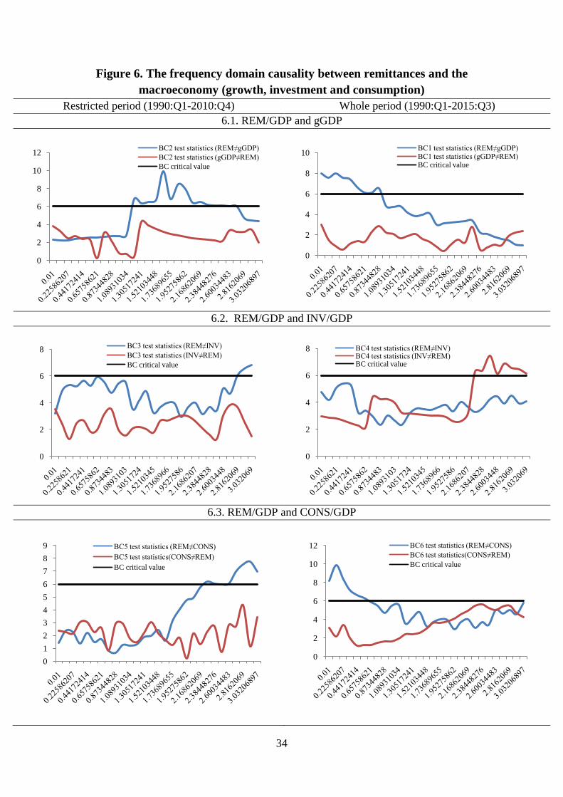
34

Figure 6. The frequency domain causality between remittances and the

macroeconomy (growth, investment and consumption)

Restricted period (1990:Q1-2010:Q4) Whole period (1990:Q1-2015:Q3)

6.1. REM/GDP and gGDP

6.2. REM/GDP and INV/GDP

6.3. REM/GDP and CONS/GDP

0

2

4

6

8

10

12BC2 test statistics (REM≠gGDP)

BC2 test statistics (gGDP≠REM)

BC critical value

0

2

4

6

8

10BC1 test statistics (REM≠gGDP)BC1 test statistics (gGDP≠REM)BC critical value

0

2

4

6

8 BC3 test statistics (REM≠INV)

BC3 test statistics (INV≠REM)

BC critical value

0

2

4

6

8 BC4 test statistics (REM≠INV)BC4 test statistics (INV≠REM)BC critical value

0

1

2

3

4

5

6

7

8

9 BC5 test statistics (REM≠CONS)

BC5 test statistics(CONS≠REM)

BC critical value

0

2

4

6

8

10

12 BC6 test statistics (REM≠CONS)

BC6 test statistics(CONS≠REM)

BC critical value

35

7. Conclusions and some policy implications

Before the downfall of Ben Ali‟s regime, Tunisia has succeeded to achieve an

average economic growth rate of almost 5 percent, a thriving tourism sector, a

dynamic manufacturing industry, a flourishing foreign trade and stable FDI inflows.

The “Arab Spring” came to underscore the weakness of the pillars of Tunisia‟s growth,

which had not withstood this untoward shock. The tourism collapsed, FDI dried up,

the foreign trade did not resist, and the dinar depreciated. Unusually, remittances

survived and even rose, highlighting their countercyclical behavior. In light of this

observation, this study attempts to determine the channels through which remittances

can help to boost economic growth in a country that saw extreme social and political

turmoil. For empirical purpose, we perform a new correlation investigation, dubbed

correlation analysis-based EMD. This technique permits to completely uncover the

hidden driving forces of the relationship between remittances and the macroeconomy

(per capita economic growth, investment and consumption) in an unstable context,

which standard techniques may be inoperable.

Because we have not enough observations to make estimation for the post-Arab

spring period, we thought to consider two periods of study: (1) prior to the aftermath

of Arab Spring, noted the restricted period, and (2) before and after the onset of Arab

Spring event or the whole period. Despite this limitation, three relevant outcomes were

drawn. First, although the remittances‟ effect on growth was negative and dominantly

determined by short-term inner factors in the restricted period, it became positive and

driven by long-term factors in the whole period. Second, while in restricted period, the

remittances‟ impact on investment was likely to be variant (negative in some scales

and positive in others) and explained by short-term inner features, in the whole period,

this effect became negative, weak and driven by short- and medium-term factors.

Third, migrants‟ remittances had a positive and significant effect on consumption in

the two periods. But, this effect held in the short-run in the restricted period and

in the long-run in the extended period.

These findings deeply suggest that it is unnecessary to oppose the two

transmission channels (consumption vs. investment) through which remittances

36

significantly affect Tunisia‟s growth. In particular, the remittance inflows were found

to be spent more on consumption-type expenditures and less on local productive

investment. Remittances may help in alleviating poverty but they did not turn the

recipients into investors, stimulating entrepreneurial activities, rising formal sector

employment, and generating multiplier effect†††

. Certainly, remittances were intended

to help families cope with the crisis, certainly they would not be channeled into

productive investment, but their positive and long-run impact on growth appeared

robust. In times of crisis, remittances will help families to feed (by consuming local

products), to heal and to continue sending their children to school; briefly, to keep

their level of consumption. However, the political and social unrest would intensify

investors‟ disquiets over the economic prospects of this country, harming the

investment climate. From an economic policy perspective, governments should

implement policies encouraging the investment use of remittances to foster the

national development process. To win back the confidence of investors, the

government is seeking to open different economic sectors to competition, to revise tax

procedures, to develop a fair administrative business environment, and more largely to

implement appropriate reforms in terms of governance and legislations.

†††

This can happen but in infrequent cases. Papers that focused on the impact of remittances

on investment seem very scarce. Generally, migrants come to invest in their country of origin

on condition that they monitor themselves their investments. For a summary of these studies,

you can refer to Bouoiyour et al. (2016).

37

References

Aggarwal, R., Demirgüç-Kunt, A and Pería, M.S.M (2006). Do workers‟ remittances

promote financial development? World Bank Policy Research Working Paper 3957.

Amuedo-Dorantes, C and Pozo, S (2004). Workers‟ remittances and the real exchange

rate: A paradox of gifts. World Development, 32(8), 1407-1417.

Bouoiyour J. (2006). Migration, Diaspora et développement humain, in « Le Maroc

possible, une offre de débat pour une ambition collective » Rapport du

cinquantenaire, 2006. Royaume du Maroc.

http://www.rdh50.ma/fr/pdf/contributions/GT3-8.PDF

Bouoiyour, J. Miftah A.and Muller C. (2016). Remittances and Living Standards in

Morocco. Working paper, CATT, University of Pau.

Bouoiyour, J. and Selmi, R. (2016 a). China‟s slowdown and Uncertainty Spillovers

within BRICS stock markets: A Signal processing analysis. Working paper, CATT,

University of Pau.

Bouoiyour J. and Selmi, R. (2016 b). Dutch Disease, Remittances and Arab Spring in

Tunisia, Working paper, CATT, University of Pau.

Breitung, J., and Candelon, B. (2006). Testing for short and long-run causality: a

frequency domain approach. Journal of Econometrics 132, 363-378.

Camarero, M. and Tamarit, C. (2002). Oil prices and Spanish competitiveness: A

cointegrated panel analysis. Journal of Policy Modeling 24(6), 591-605.

Carrera, J. E. and Restout, R. (2008). Long Run Determinants of Real Exchange Rates

in Latin America. Working paper GATE 08-11.

Central Bank of Tunisia (2014). La balance des paiements et la position extérieure

globale de la Tunisie 2013.

Chami, R, Fullenkamp, C, and Jahjah, S. (2005). Are immigrant remittance flows a

source of capital for development? IMF Staff Papers, 52(1), 55-81.

Barajas, A, Chami, R, Fullenkamp, C, Gapen, M and Montiel, M. (2009). Do

workers‟ remittances promote economic growth? IMF Working Paper 09/153,

Washington, D.C. International Monetary Fund.

Drazin, P. G. (1992). Nonlinear systems. Cambridge University Press.

38

Geweke, J. (1982). Measurement of linear dependence and feedback between multiple

time series. Journal of American Statistical Association 77, 304-324.

Granger, C.W.J. (1969), Investigation causal relations by econometric models and

cross-spectral methods. Econometrica 37, 424-438.

Gubert , F., Lassourd, T. and Mesplé-Somps, S. (2010). Do remittances affect poverty

and inequality? Evidence from Mali. Dauphine Working Paper.

Giuliano, P and Ruiz-Arranz, M (2009). Remittances, financial development, and

growth. Journal of Development Economics 90, 144-152.

Huang, N.E., Z. Shen, S. R. Long, M. C. Wu, H. H. Shih, Q. Zheng, N.-C. Yen, C. C.

Tung, and H. H. Liu. (1998). The Empirical Mode Decomposition and Hilbert

Spectrum for Nonlinear and Nonstationary Time Series Analysis. Proceedings of

the Royal Society London A., 454:903–995.

Huang, N. E. and N. O. Attoh-Okine, (2005), “Hilbert-Huang Transform in

Engineering.” CRC Press.

IOM (2011). Quels liens les tunisiens résidant en Europe gardent-ils avec le pays

d‟origine ? In the project TIDO “Tunisian migrants Involved in Development of

the country of Origin”.

Kifle, T. (2007). Do Remittances Encourage Investment in Education? Evidence from

Eritrea. Journal of African studies, 4(1).

Lin, L., and J. Hongbing, J. (2009). Signal feature extraction based on an

improved EMD method”, Measurement, 42 (5), 796-803.

Litterman, R.B. and Weiss, L. (1983). Money, real interest rates, and output: a

reinterpretation of postwar U.S. data. NBER working paper series n°1077.

Lueth E and Ruiz-Arranz, M. (2007). Are Workers‟ Remittances a Hedge Against

Macroeconomic Shocks? The Case of Sri Lanka. IMF, WP/ 07/22.

Mansuri, G. (2006). Migration, school attainment, and child labor: evidence from rural

Pakistan. Policy Research Working Paper Series 3945, World Bank.

McCormick, B and Wahba, J. (2003). Overseas work experience, savings and

entrepreneurship amongst return migrants to LDCs. Journal of African economies,

12 (4), 500-532.

39

Mesnard, A. (2004). Temporary migration and capital market imperfections. Oxford

Economic Papers, 56(2), 242-262.

Ng, S. and Perron, P. (2001). Lag Length Selection and the Construction of Unit Root

Tests with Good Size and Power. Econometrica 69(6), 1519-1554.

Fayissa, B and Nsiah, C. (2008). The impact of remittances on economic growth and

development in Africa. Working Paper Series, Middle Tennessee State University.

Fayissa, B and Nsiah, C. (2010). Can remittances spur economic growth and

development? Evidence from Latin American Countries. Department of Economics

and Finance Working Paper Series, Middle Tennessee State University.

Giuliano, P and Ruiz-Arranz, M. (2009). Remittances, financial development, and

growth. Journal of Development Economics 90, 144-152.

Glytsos, N.P. (2002). Dynamic effects of migrant remittances on growth: An

Econometric Model with an application to Mediterranean Countries. Centre Of

Planning And Economic Research No 74.

Özden, C and Schiff, M. (2006). Overview. In C. Özden & M. Schiff (Eds.),

International migration, remittances & the brain drain (1-18). Washington, DC:

World Bank and Palgrave Macmillan.

OECD (2013). World Migration in Figures. A joint contribution by UN-DESA and the

OECD to the United Nations High-Level Dialogue on Migration and Development,

3-4 October.

Pollack, K.M. (2011). Understanding the Arab awakening.

http://www.brookings.edu/~/media/press/books/2011/thearabawakening/thearabawake

ning_chapter.pdf

Rao, B and Hassan, G. (2010). Are Direct and Indirect Growth Effects of Remittances

Significant? In 6th Annual Australasian Development Economics Workshop.

Rydges Hotel, Parramatta: UWS.

Sims, C.A. (1980). Macroeconomics and Reality. Econometrica, 48, 1-48.

Valero-Gil, J (2008). Remittances and the household‟s expenditures on health. MPRA

Paper 9572, University Library of Munich, Germany.

Woodruff, C and Zenteno, R. (2004). Remittances and microenterprises in Mexico.

Graduate School of International Relations and Pacific Studies Working Paper.

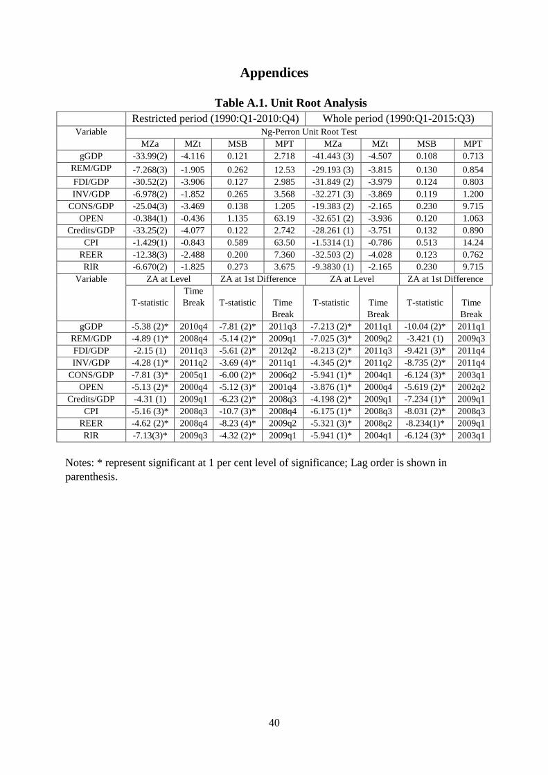
40

Appendices

Table A.1. Unit Root Analysis

Restricted period (1990:Q1-2010:Q4) Whole period (1990:Q1-2015:Q3)

Variable Ng-Perron Unit Root Test

MZa MZt MSB MPT MZa MZt MSB MPT

gGDP -33.99(2) -4.116 0.121 2.718 -41.443 (3) -4.507 0.108 0.713

REM/GDP -7.268(3) -1.905 0.262 12.53 -29.193 (3) -3.815 0.130 0.854

FDI/GDP -30.52(2) -3.906 0.127 2.985 -31.849 (2) -3.979 0.124 0.803

INV/GDP -6.978(2) -1.852 0.265 3.568 -32.271 (3) -3.869 0.119 1.200

CONS/GDP -25.04(3) -3.469 0.138 1.205 -19.383 (2) -2.165 0.230 9.715

OPEN -0.384(1) -0.436 1.135 63.19 -32.651 (2) -3.936 0.120 1.063

Credits/GDP -33.25(2) -4.077 0.122 2.742 -28.261 (1) -3.751 0.132 0.890

CPI -1.429(1) -0.843 0.589 63.50 -1.5314 (1) -0.786 0.513 14.24

REER -12.38(3) -2.488 0.200 7.360 -32.503 (2) -4.028 0.123 0.762

RIR -6.670(2) -1.825 0.273 3.675 -9.3830 (1) -2.165 0.230 9.715

Variable ZA at Level ZA at 1st Difference ZA at Level ZA at 1st Difference

T-statistic

Time

Break

T-statistic

Time

Break

T-statistic

Time

Break

T-statistic

Time

Break

gGDP -5.38 (2)* 2010q4 -7.81 (2)* 2011q3 -7.213 (2)* 2011q1 -10.04 (2)* 2011q1

REM/GDP -4.89 (1)* 2008q4 -5.14 (2)* 2009q1 -7.025 (3)* 2009q2 -3.421 (1) 2009q3

FDI/GDP -2.15 (1) 2011q3 -5.61 (2)* 2012q2 -8.213 (2)* 2011q3 -9.421 (3)* 2011q4

INV/GDP -4.28 (1)* 2011q2 -3.69 (4)* 2011q1 -4.345 (2)* 2011q2 -8.735 (2)* 2011q4

CONS/GDP -7.81 (3)* 2005q1 -6.00 (2)* 2006q2 -5.941 (1)* 2004q1 -6.124 (3)* 2003q1

OPEN -5.13 (2)* 2000q4 -5.12 (3)* 2001q4 -3.876 (1)* 2000q4 -5.619 (2)* 2002q2

Credits/GDP -4.31 (1) 2009q1 -6.23 (2)* 2008q3 -4.198 (2)* 2009q1 -7.234 (1)* 2009q1

CPI -5.16 (3)* 2008q3 -10.7 (3)* 2008q4 -6.175 (1)* 2008q3 -8.031 (2)* 2008q3

REER -4.62 (2)* 2008q4 -8.23 (4)* 2009q2 -5.321 (3)* 2008q2 -8.234(1)* 2009q1

RIR -7.13(3)* 2009q3 -4.32 (2)* 2009q1 -5.941 (1)* 2004q1 -6.124 (3)* 2003q1

Notes: * represent significant at 1 per cent level of significance; Lag order is shown in

parenthesis.

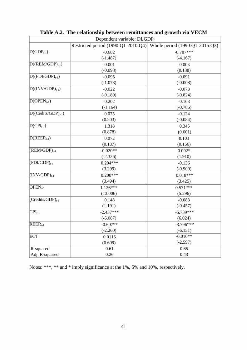
41

Table A.2. The relationship between remittances and growth via VECM

Dependent variable: DLGDPt

Restricted period (1990:Q1-2010:Q4) Whole period (1990:Q1-2015:Q3)

D(GDPt-1)

-0.682

(-1.487)

-0.787***

(-4.167)

D((REM/GDP)t-1)

-0.001

(-0.098)

0.003

(0.138)

D((FDI/GDP)t-1)

-0.095

(-1.078)

-0.091

(-0.008)

D((INV/GDP)t-1)

-0.022

(-0.180)

-0.073

(-0.824)

D(OPENt-1)

-0.202

(-1.164)

-0.163

(-0.786)

D((Cedits/GDP)t-1)

0.075

(0.203)

-0.124

(-0.084)

D(CPIt-1)

1.318

(0.878)

0.345

(0.601)

D(REERt-1)

0.072

(0.137)

0.103

(0.156)

(REM/GDP)t-1

-0.020**

(-2.326)

0.092*

(1.910)

(FDI/GDP)t-1

0.204***

(3.299)

-0.136

(-0.900)

(INV/GDP)t-1

0.200***

(3.494)

0.018***

(3.425)

OPENt-1

1.126***

(13.006)

0.571***

(5.296)

(Credits/GDP)t-1

0.148

(1.191)

-0.083

(-0.457)

CPIt-1

-2.437***

(-5.087)

-5.739***

(6.024)

REERt-1

-0.607**

(-2.260)

-3.796***

(-6.151)

ECT

0.0115

(0.609)

-0.010**

(-2.597)

R-squared

Adj. R-squared

0.61

0.26

0.65

0.43

Notes: ***, ** and * imply significance at the 1%, 5% and 10%, respectively.

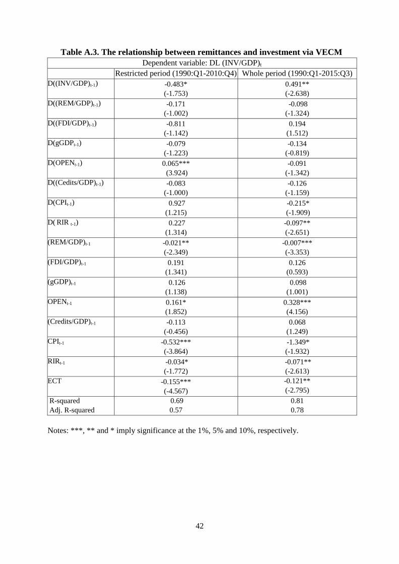
42

Table A.3. The relationship between remittances and investment via VECM

Dependent variable: DL (INV/GDP)t

Restricted period (1990:Q1-2010:Q4) Whole period (1990:Q1-2015:Q3)

D((INV/GDP)t-1)

-0.483*

(-1.753)

0.491**

(-2.638)

D((REM/GDP)t-1)

-0.171

(-1.002)

-0.098

(-1.324)

D((FDI/GDP)t-1)

-0.811

(-1.142)

0.194

(1.512)

D(gGDPt-1)

-0.079

(-1.223)

-0.134

(-0.819)

D(OPENt-1)

0.065***

(3.924)

-0.091

(-1.342)

D((Cedits/GDP)t-1)

-0.083

(-1.000)

-0.126

(-1.159)

D(CPIt-1)

0.927

(1.215)

-0.215*

(-1.909)

D( RIR t-1)

0.227

(1.314)

-0.097**

(-2.651)

(REM/GDP)t-1

-0.021**

(-2.349)

-0.007***

(-3.353)

(FDI/GDP)t-1

0.191

(1.341)

0.126

(0.593)

(gGDP)t-1

0.126

(1.138)

0.098

(1.001)

OPENt-1

0.161*

(1.852)

0.328***

(4.156)

(Credits/GDP)t-1

-0.113

(-0.456)

0.068

(1.249)

CPIt-1

-0.532***

(-3.864)

-1.349*

(-1.932)

RIRt-1

-0.034*

(-1.772)

-0.071**

(-2.613)

ECT

-0.155***

(-4.567)

-0.121**

(-2.795)

R-squared

Adj. R-squared

0.69

0.57

0.81

0.78

Notes: ***, ** and * imply significance at the 1%, 5% and 10%, respectively.

43

Table A.4. The relationship between remittances and consumption via VECM

Dependent variable: DL (CONS/GDP)t

Restricted period (1990:Q1-2010:Q4) Whole period (1990:Q1-2015:Q3)

D((CONS/GDP)t-1)

0.157**

(2.223)

0.413***

(3.879)

D((REM/GDP)t-1)

-0.098

(-0.776)

-0.093

(-1.424)

D((Cedits/GDP)t-1)

-0.141

(-1.511)

-0.100**

(-2.296)

D(gGDPt-1)

-0.056

(-1.416)

-0.083

(-1.176)

D(RIRt-1)

-0.098

(-1.367)

-0.094

(-1.312)

D(CPIt-1)

-0.134**

(-1.798)

-0.116***

(-3.714)

(REM/GDP)t-1

-0.014*

(-1.986)

0.097**

(2.364)

(Credits/GDP)t-1

- 0.081**

(-3.025)

-0.123**

(-2.515)

(gGDP)t-1

0.034

(1.161)

0.034*

(1.823)

RIRt-1

-0.215***

(-3.911)

-0.236***

(-4.812)

CPIt-1

-0.167**

(-2.197)

-0.214***

(-4.581)

ECT

-0.123

(-1.495)

-0.095

(-1.246)

R-squared

Adj. R-squared

0.46

0.40

0.51

0.47

Notes: ***, ** and * imply significance at the 1%, 5% and 10%, respectively.

Table A. 5. The relationship between remittances and macroeconomy (growth,

investment and consumption) via standard Granger causality tests

Restricted period (1990:Q1-2010:Q4) Whole period (1990:Q1-2015:Q3)

gGDP INV/GDP CONS/GDP gGDP INV/GDP CONS/GDP

REM/GDP 0.1051 0.0814* 0.2568 0.0623* 0.0945* 0.0372*

Notes: p-value<0.01: ***; p-value<0.05: **; p-value<0.1.

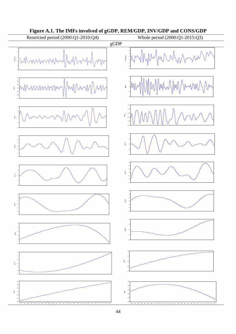
44

Figure A.1. The IMFs involved of gGDP, REM/GDP, INV/GDP and CONS/GDP

Restricted period (2000:Q1-2010:Q4) Whole period (2000:Q1-2015:Q3)

gGDP

-2

-1

0

1

2

3

Ori

gin

al

-1.2

-0.8

-0.4

0.0

0.4

0.8

1.2

IMF

1

-.8

-.4

.0

.4

.8

IMF

2

-.6

-.4

-.2

.0

.2

.4

.6

IMF

3

-.4

-.2

.0

.2

.4

IMF

4

-.3

-.2

-.1

.0

.1

.2

.3

IMF

5

.0

.1

.2

.3

.4

.5

IMF

6

-.5

-.4

-.3

-.2

-.1

.0

.1

IMF

7

-.55

-.50

-.45

-.40

-.35

-.30

-.25

90 91 92 93 94 95 96 97 98 99 00 01 02 03 04 05 06 07 08 09 10 11 12 13 14 15

RE

S

-2

-1

0

1

2

3

4

5

Ori

gin

al

-2

-1

0

1

2

IMF

1-1.0

-0.5

0.0

0.5

1.0

1.5

IMF

2

-.8

-.4

.0

.4

.8

IMF

3

-.3

-.2

-.1

.0

.1

.2

.3

IMF

4

-.6

-.4

-.2

.0

.2

.4

.6

IMF

5

-.4

-.2

.0

.2

.4

IMF

6

-.4

-.2

.0

.2

.4

IMF

7

.08

.09

.10

.11

.12

.13

90 91 92 93 94 95 96 97 98 99 00 01 02 03 04 05 06 07 08 09 10 11 12 13 14 15

RES

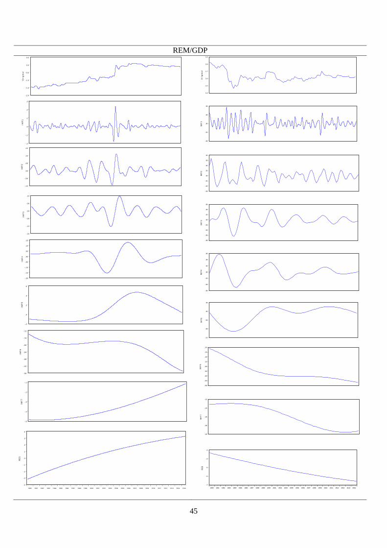
45

REM/GDP

-2 .0

-1 .5

-1 .0

-0 .5

0.0

0.5

Orig

ina

l

- .2

- .1

.0

.1

.2

.3

IM

F1

- .10

- .05

.00

.05

.10

.15

IM

F2

- .15

- .10

- .05

.00

.05

.10

IM

F3

- .20

- .15

- .10

- .05

.00

.05

.10

.15

IM

F4

- .2

.0

.2

.4

.6

IM

F5

- .96

- .92

- .88

- .84

- .80

- .76

- .72

IM

F6

- .5

- .4

- .3

- .2

- .1

IM

F7

- .4

- .3

- .2

- .1

.0

.1

.2

.3

.4

1990 1991 1992 1993 1994 1995 1996 1997 1998 1999 2000 2001 2002 2003 2004 2005 2006 2007 2008 2009 2010 2011 2012 2013 2014 2015

RE

S

1.4

1.5

1.6

1.7

1.8

1.9

Orig

ina

l

-.04

-.02

.00

.02

.04

IMF

1

-.03

-.02

-.01

.00

.01

.02

.03

.04

IMF

2

-.08

-.06

-.04

-.02

.00

.02

.04

.06

IMF

3

-.06

-.04

-.02

.00

.02

.04

.06

IMF

4

-.12

-.08

-.04

.00

.04

IMF

5

-.08

-.04

.00

.04

.08

.12

.16

.20

.24

IMF

6

-.20

-.18

-.16

-.14

-.12

IMF

7

-.7

-.6

-.5

-.4

-.3

1990 1991 1992 1993 1994 1995 1996 1997 1998 1999 2000 2001 2002 2003 2004 2005 2006 2007 2008 2009 2010 2011 2012 2013 2014 2015

RE

S

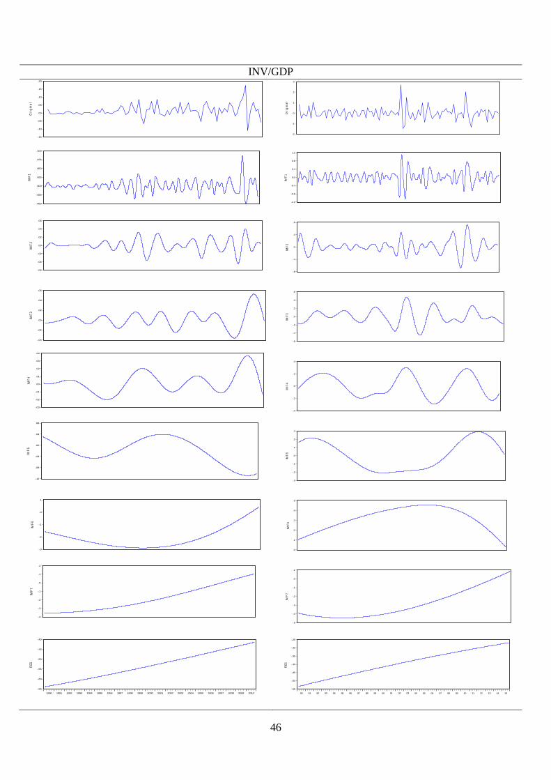
46

INV/GDP

-.15

-.10

-.05

.00

.05

.10

.15

.20

Ori

gin

al

-.050

-.025

.000

.025

.050

.075

.100

IMF

1

-.06

-.04

-.02

.00

.02

.04

.06

IMF

2

-.04

-.02

.00

.02

.04

.06

IMF

3

-.03

-.02

-.01

.00

.01

.02

.03

.04

IMF

4

-.12

-.08

-.04

.00

.04

.08

IMF

5

-.3

-.2

-.1

.0

.1

IMF

6

-.4

-.3

-.2

-.1

.0

.1

.2

IMF

7

-.65

-.60

-.55

-.50

-.45

-.40

1990 1991 1992 1993 1994 1995 1996 1997 1998 1999 2000 2001 2002 2003 2004 2005 2006 2007 2008 2009 2010

RE

S

-2

-1

0

1

2

3

Ori

gin

al

-1.2

-0.8

-0.4

0.0

0.4

0.8

1.2

IMF

1

-.8

-.4

.0

.4

.8

IMF

2

-.6

-.4

-.2

.0

.2

.4

.6

IMF

3

-.4

-.2

.0

.2

.4

IMF

4

-.3

-.2

-.1

.0

.1

.2

.3

IMF

5

.0

.1

.2

.3

.4

.5

IMF

6

-.5

-.4

-.3

-.2

-.1

.0

.1

IMF

7

-.55

-.50

-.45

-.40

-.35

-.30

-.25

90 91 92 93 94 95 96 97 98 99 00 01 02 03 04 05 06 07 08 09 10 11 12 13 14 15

RE

S

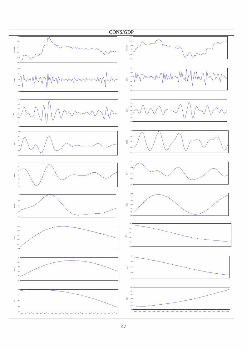
47

CONS/GDP

1.6

2.0

2.4

2.8

3.2

3.6

Ori

gin

al

-.2

-.1

.0

.1

.2

IMF

1

-.12

-.08

-.04

.00

.04

.08

.12

IMF

2

-.2

-.1

.0

.1

.2

.3

IMF

3

-.3

-.2

-.1

.0

.1

.2

.3

IMF

4

-.1

.0

.1

.2

.3

IMF

5

0.0

0.2

0.4

0.6

0.8

1.0

IMF

6

.20

.25

.30

.35

.40

.45

IMF

7

.28

.32

.36

.40

.44

90 91 92 93 94 95 96 97 98 99 00 01 02 03 04 05 06 07 08 09 10 11 12 13 14 15

RES

2.35

2.40

2.45

2.50

2.55

2.60

Ori

gin

al

-.03

-.02

-.01

.00

.01

.02

IMF

1

-.03

-.02

-.01

.00

.01

.02

.03

IMF

2

-.02

-.01

.00

.01

.02

IMF

3

-.02

-.01

.00

.01

.02

IMF

4

-.06

-.04

-.02

.00

.02

.04

.06

IMF

5

-.15

-.10

-.05

.00

.05

.10

IMF

6

-.4

-.3

-.2

-.1

.0

IMF

7

-.78

-.76

-.74

-.72

-.70

-.68

-.66

1990 1991 1992 1993 1994 1995 1996 1997 1998 1999 2000 2001 2002 2003 2004 2005 2006 2007 2008 2009 2010

RE

S

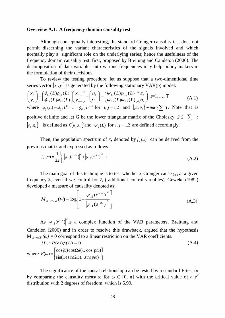
48

Overview A.1. A frequency domain causality test

Although conceptually interesting, the standard Granger causality test does not

permit discerning the variant characteristics of the signals involved and which

normally play a significant role on the underlying series; hence the usefulness of the

frequency domain causality test, first, proposed by Breitung and Candelon (2006). The

decomposition of data variables into various frequencies may help policy makers in

the formulation of their decisions.

To review the testing procedure, let us suppose that a two-dimentional time

series vector tt yx , is generated by the following stationary VAR(p) model:

t

t

t

t

t

t

y

x

LL

LL

y

x

1

1

2221

1211

)()(

)()(

t

t

LL

LL

)()(

)()(

2221

1211 ,t=1,…, T (A.1)

where 1

,

0

1, ...)( p

pijijij LLL for 2,1, ji

and ', tt ∼ ),0( iid . Note that is

positive definite and let G be the lower triangular matrix of the Cholesky 1

'

GG ;

', tt is defined as ', ttG and )(Lij for 2,1, ji are defined accordingly.

Then, the population spectrum of x, denoted by )(xf , can be derived from the

previous matrix and expressed as follows:

2

12

2

11 )()(2

1)(

ii

x eef (A.2)

The main goal of this technique is to test whether xt Granger cause yt , at a given

frequency λ, even if we control for Zt ( additional control variables). Geweke (1982)

developed a measure of causality denoted as:

2

11

2

12

/

)(

)(1log)(

iw

iw

Zyx

e

ewM

(A.3)

As 2

12 )( iwe is a complex function of the VAR parameters, Breitung and

Candelon (2006) and in order to resolve this drawback, argued that the hypothesis

M x→y/Z (ω) = 0 correspond to a linear restriction on the VAR coefficients.

0)()(:0 LRH (A.4)

where

)sin()...2sin()sin(

)cos()...2cos()cos()(

p

pR

The significance of the causal relationship can be tested by a standard F-test or

by comparing the causality measure for ω ∈ [0, π] with the critical value of a χ2

distribution with 2 degrees of freedom, which is 5.99.