Relationships of HMA In-Place Air Voids, Lift Thickness ...onlinepubs.trb.org/onlinepubs/nchrp/nchrp_w68v1.pdf · Voids, Lift Thickness, and Permeability Prepared for: National Cooperative

NCHRP Web Document 68 (Project 9-27)

Relationships of HMA In-Place Air

Voids, Lift Thickness, and Permeability

Prepared for:

National Cooperative Highway Research Program

Submitted by:

E. Ray Brown

M. Rosli Hainin Allen Cooley

Graham Hurley National Center for Asphalt Technology

Auburn University Auburn, Alabama

September 2004

Volume One

ACKNOWLEDGMENT This work was sponsored by the American Association of State Highway and Transportation Officials (AASHTO), in cooperation with the Federal Highway Administration, and was conducted in the National Cooperative Highway Research Program (NCHRP), which is administered by the Transportation Research Board (TRB) of the National Academies.

DISCLAIMER The opinion and conclusions expressed or implied in the report are those of the research agency. They are not necessarily those of the TRB, the National Research Council, AASHTO, or the U.S. Government. This report has not been edited by TRB.

The National Academy of Sciences is a private, nonprofit, self-perpetuating society of distinguished scholars engaged in scientific and engineering research, dedicated to the furtherance of science and technology and to their use for the general welfare. On the authority of the charter granted to it by the Congress in 1863, the Academy has a mandate that requires it to advise the federal government on scientific and technical matters. Dr. Bruce M. Alberts is president of the National Academy of Sciences. The National Academy of Engineering was established in 1964, under the charter of the National Academy of Sciences, as a parallel organization of outstanding engineers. It is autonomous in its administration and in the selection of its members, sharing with the National Academy of Sciences the responsibility for advising the federal government. The National Academy of Engineering also sponsors engineering programs aimed at meeting national needs, encourages education and research, and recognizes the superior achievements of engineers. Dr. William A. Wulf is president of the National Academy of Engineering. The Institute of Medicine was established in 1970 by the National Academy of Sciences to secure the services of eminent members of appropriate professions in the examination of policy matters pertaining to the health of the public. The Institute acts under the responsibility given to the National Academy of Sciences by its congressional charter to be an adviser to the federal government and, on its own initiative, to identify issues of medical care, research, and education. Dr. Harvey V. Fineberg is president of the Institute of Medicine. The National Research Council was organized by the National Academy of Sciences in 1916 to associate the broad community of science and technology with the Academy’s purposes of furthering knowledge and advising the federal government. Functioning in accordance with general policies determined by the Academy, the Council has become the principal operating agency of both the National Academy of Sciences and the National Academy of Engineering in providing services to the government, the public, and the scientific and engineering communities. The Council is administered jointly by both the Academies and the Institute of Medicine. Dr. Bruce M. Alberts and Dr. William A. Wulf are chair and vice chair, respectively, of the National Research Council. The Transportation Research Board is a division of the National Research Council, which serves the National Academy of Sciences and the National Academy of Engineering. The Board’s mission is to promote innovation and progress in transportation through research. In an objective and interdisciplinary setting, the Board facilitates the sharing of information on transportation practice and policy by researchers and practitioners; stimulates research and offers research management services that promote technical excellence; provides expert advice on transportation policy and programs; and disseminates research results broadly and encourages their implementation. The Board's varied activities annually engage more than 5,000 engineers, scientists, and other transportation researchers and practitioners from the public and private sectors and academia, all of whom contribute their expertise in the public interest. The program is supported by state transportation departments, federal agencies including the component administrations of the U.S. Department of Transportation, and other organizations and individuals interested in the development of transportation. www.TRB.org

www.national-academies.org

i

TABLE OF CONTENTS

Page

LIST OF TABLES……………………………………………………………………………… iv

LIST OF FIGURES ..………………………………………...………………………...……… viii

1.0 INTRODUCTION AND PROBLEM STATEMENT…………………………………… 1

2.0 OBJECTIVE……………………………………………………………………………. 3

3.0 RESEARCH APPROACH………………………………………………………………. 3

3.1 Part 1 – Experimental Plan ……………………………………………………… 6

3.1.1 Evaluation of Effect of t/NMAS on Density Using

Gyratory Compactor…………………………………………………...… 6

3.1.2 Evaluation of Effect of t/NMAS on Density Using

Vibratory Compactor ……………………………………………………10

3.1.3 Evaluation of Effect of t/NMAS on Density Using Field Experiment.. ...11

3.1.4 Evaluation of Effect of Temperature on Relationship Between Density

and t/NMAS from Field Experiment ….………………………………...14

3.1.5 Evaluation of Effect of t/NMAS on Permeability Using Gyratory

Compactor ……………………………………………………………… 14

3.1.6 Evaluation of Effect of t/NMAS on Permeability Using Vibratory

Compactor …………………………………………………………..….. 15

3.1.7 Evaluation of Effect of t/NMAS on Permeability Using Field

Experiment ……..………………………………………………………. 15

VOLUME ONE

ii

3.2 Part 2 Experimental Plan – Evaluation of Relationship of Laboratory

Permeability, In-place Air Voids, and Lift Thickness of Field Compacted Cores

(NCHRP 9-9(1))………………………………………………………………... 16

4.0 MATERIALS AND TEST METHODS ………………………………………………. 17

4.1 Aggregate and Binder Properties ………………………………………………. 17

4.2 Aggregate Gradations ………………………………………………………….. 19

4.3 Determination of Bulk Specific Gravity ………………………………………...23

4.4 Determination of Permeability …………………………………………….…….24

4.5 Part 2 – Evaluation of Relationship of Laboratory Permeability, Density,

and Lift Thickness of Field Compacted Cores ………………………………….24

5.0 TEST RESULTS AND ANALYSIS ……………………………………………………25

5.1 Part 1- Mix Designs ……………………………………………………………..25

5.2 Evaluation of Effect of t/NMAS on Density Using Gyratory Compactor ………32

5.3 Evaluation of Effect of t/NMAS on Density Using Vibratory Compactor………48

5.4 Evaluation of Effect of t/NMAS on Density from Field Study……. ..………… 61

5.4.1 Section 1 ………………………………………………………………... 61

5.4.2 Section 2 ……………………………………………………………….. 64

5.4.3 Section 3 ………………………………………………………………. 68

5.4.4 Section 4 ………………………………………………………………. 71

5.4.5 Section 5 ………………………………………………………………. 75

5.4.6 Section 6 ………………………………………………………………. 77

5.4.7 Section 7 ………………………………………………………………. 80

5.5 Evaluation of the Effect of Temperature on the Relationships Between Density

iii

and t/NMAS from the Field Experiment .…………………………....………… 84

5.6 Evaluation of Effect of t/NMAS on Permeability Using Gyratory Compacted

Specimen Experiment………………………………………………………... …91

5.7 Evaluation of Effect of t/NMAS on Permeability Using Laboratory

Vibratory Compacted Specimen...…………………………………………….…93

5.8 Evaluation of Effect of t/NMAS on Permeability from Field Study……......….. 93

5.8.1 Section 1- 9.5mm Fine-Graded HMA…..………………………….…. 94

5.8.2 Section 2 - 9.5mm Coarse-Graded HMA.………………………….…. 97

5.8.3 Section 3 - 9.5mm SMA………………………………………….…… 100

5.8.4 Section 4 - 12.5 SMA………………………………….………….…… 102

5.8.5 Section 5 - 19.0mm Fine-Graded ………………………………….… 106

5.8.6 Section 6 - 19.0mm Coarse-Graded ……………………………….…. 108

5.8.7 Section 7 - 19.0mm Coarse-Graded with Modified Asphalt………. ... 110

5.9 Part 2 – Evaluation of Relationship of Laboratory Permeability, Density,

and Lift Thickness of Field Compacted Cores ……………………………...…114

6.0 DISCUSSION OF RESULTS.…………………………………………………………121

6.1 Determination of Minimum t/NMAS.……………………………………….…121

6.2 Effect of Mix Temperature on Compaction ……………………………………124

6.3 Effect of Thickness on Permeability at 7.0 ± 1.0 percent Air Voids ...………….125

6.4 Evaluation on Factors Affecting Permeability ………………………………...125

7.0 CONCLUSIONS ………………………………………………………………………126

8.0 REFERENCES ………………………………………………………………………...127

iv

LIST OF TABLES

Page

Table 1: Mix Information for Field Density Study ……………………………….. 12

Table 2: Physical Properties of Aggregate ……………………………………….. 18

Table 3: Asphalt Binder Properties ………………………………………………. 19

Table 4: Mix Information for Field Study ………………………………………. 22

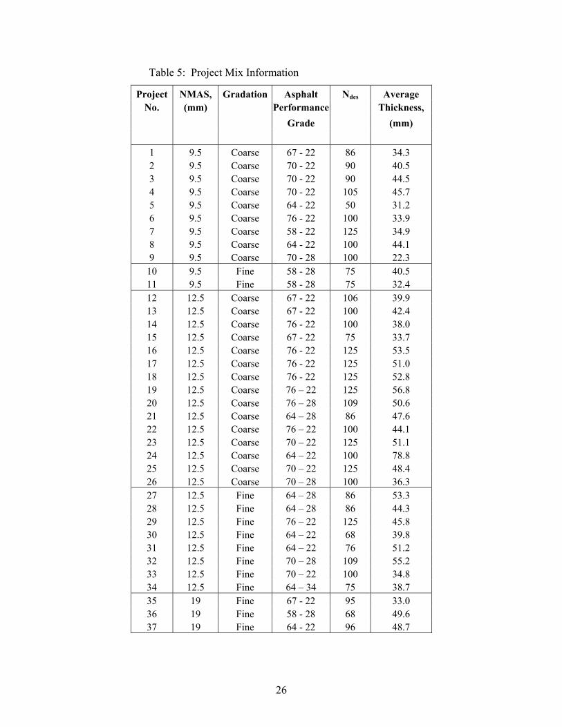
Table 5: Project Mix Information for Field Compacted Cores …………………… 26

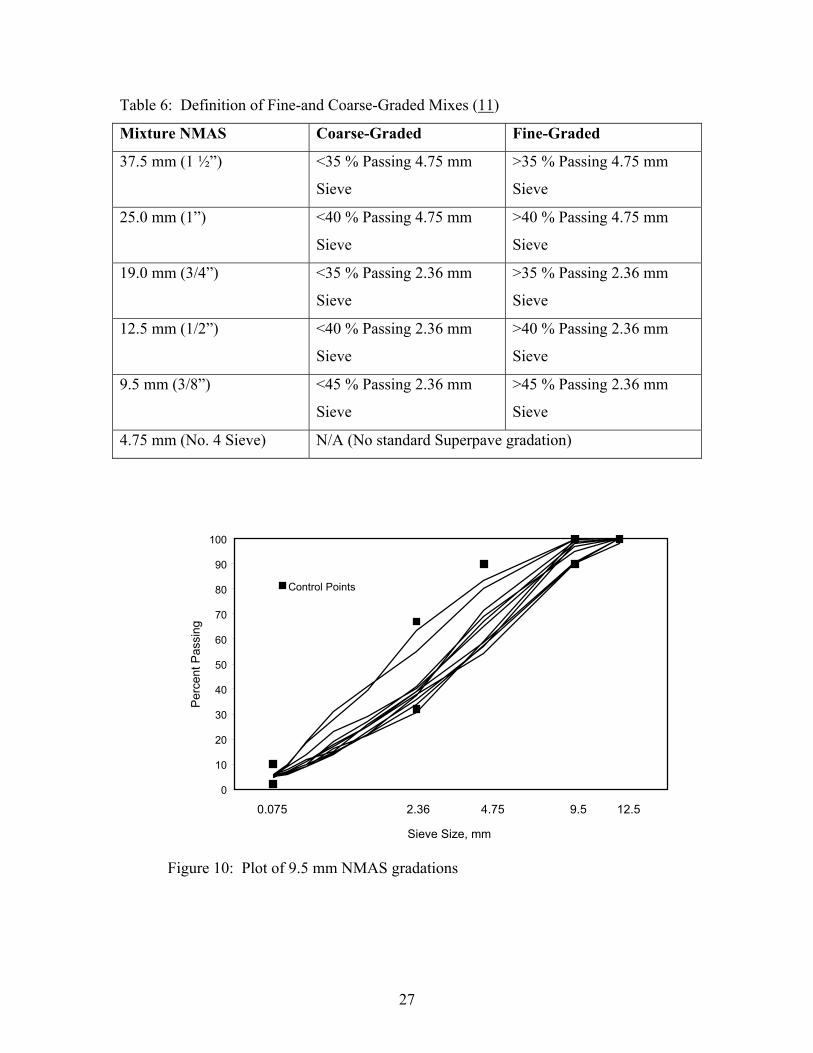
Table 6: Definition of Fine- and Coarse-Graded Mixes (11) …………………….. 27

Table 7: Summary of Mix Design Results for Superpave Mixes ………………… 29

Table 8: Summary of Mix Design Results for SMA Mixes ……………………… 30

Table 9: Change of Gradation for 9.5 mm NMAS Superpave Mixes …………… 30

Table 10: Change of Gradation for 19.0 mm NMAS Superpave Mixes …………. 31

Table 11: Change of Gradation for SMA Mixes ………………………………… 31

Table 12: Results for Granite Mixes …………………………………………….. 34

Table 13: Results for Limestone Mixes ………………………………………….. 35

Table 14: Results for Gravel Mixes …………………………………………….. 36

Table 15: ANOVA of Air Voids for Superpave Mixes …………………………. 40

Table 16: ANOVA of Air Voids for SMA Mixes ………………………………. 40

Table 17: Summary of Minimum t/NMAS to Provide 7.0 % Air Voids

in Laboratory ………………………………………………………..… 48

Table 18: Results of Air Voids for Limestone Superpave Mixes ………………… 50

Table 19: Results of Air Voids for Granite Superpave Mixes ………….………… 51

Table 20: ANOVA of Air Voids for Superpave Mixes …………………………. 53

v

Table 21: ANOVA of Air Voids for SMA Mixes ………………………………. 54

Table 22: Summary of Minimum t/NMAS Using Laboratory

Vibratory Compactor …………………………………………………… 60

Table 23 Thickness, t/NMAS, Air Voids and Water Absorption for Section 1…… 62

Table 24 Thickness, t/NMAS, Air Voids and Water Absorption for Section 2

Steel Wheel Roller……………………………….………….…… 66


Steel/Rubber Tire Roller………………………………….………….… 66


Steel Wheel Roller……………………………….………….………… 70




Steel Wheel Roller……………………………….………….……….… 73


Steel/Rubber Tire Roller………………………….………………..….… 74


Steel Wheel Roller……………………………….………….………..… 76






vi




Table 35: T/NMAS, Temperature at 20 min., Asphalt Type and Difference in

Temperature…………………………………………………………… 85

Table 36: Results of Permeability Testing Using Gyratory Compactor ………… 92

Table 37: Results of Permeability Testing Using Vibratory Compactor ………… 94

Table 38: Permeability Results for 9.5 mm Fine-Graded –Steel Roller …………. 95

Table 39: Permeability Results for 9.5 mm Coarse-Graded –Steel Roller ………. 98

Table 40: Permeability Results for 9.5 mm Coarse-Graded –Steel/RubberTire …. 98

Table 41: Permeability Results for 9.5 mm SMA –Steel Roller ……………….…. 100

Table 42: Permeability Results for 9.5 mm SMA –Steel/RubberTire ……………. 101

Table 43: Permeability Results for 12.5 mm SMA –Steel Roller ………………….103

Table 44: Permeability Results for 12.5 mm SMA –Steel/RubberTire ………….... 104

Table 45: Permeability Results for 19.0 mm Fine-Graded –Steel Roller ………… 106

Table 46: Permeability Results for 19.0 mm Coarse-Graded –Steel Roller………. 108

Table 47: Permeability Results for 19.0 mm Coarse-Graded –Steel/Rubber Tire... 109

Table 48: Permeability Results for 19.0 mm Coarse-Graded

with Modified Asphalt –Steel Roller………………………………….... 111

Table 49: Permeability Results for 19.0 mm Coarse-Graded

With Modified Asphalt –Steel/Rubber Tire Roller……………….……. 112

Table 50: Average Air Voids, Water Absorption and Permeability

For Field Projects ……………………………………………………… 115

vii

Table 51: Best Subsets Regression on Factors Affecting Permeability …………. 120

Table 52: Effect of t/NMAS on Compactibility of HMA…………..…………… 122

viii

LIST OF FIGURES

Page

Figure 1: Experimental Plan for Part 1 of Task 3 ………………………………… 4

Figure 2: Experimental Plan for Field Study……………………………………… 7

Figure 3: Experimental Plan for Part 2 …………………………………………… 8

Figure 4: Thermocouple Location in Asphalt Mat ………………………………. 13

Figure 5: Permeability Test Conducted at Each Location ……………………….. 16

Figure 6: 9.5 mm NMAS Superpave Gradations ………………………………… 20

Figure 7: 19.0 mm NMAS Superpave Gradations ………………………………. 20

Figure 8: 37.5 mm NMAS Superpave Gradations ……………………………….. 21

Figure 9: SMA Gradations ……………………..………………………………… 21

Figure 10: Plot of 9.5 mm NMAS Gradations …………………………………… 27

Figure 11: Plot of 12.5 mm NMAS Gradations ………………………………… 28

Figure 12: Plot of 19.0 mm NMAS Gradations ………………………………… 28

Figure 13: Relationship Between Air Voids for ARZ Mixes……………………. 37

Figure 14: Relationship Between Air Voids for TRZ Mixes…………………….. 37

Figure 15: Relationship Between Air Voids for BRZ Mixes…………………….. 38

Figure 16: Relationship Between Air Voids for SMA Mixes…………………….. 38

Figure 17: Relationships of t/NMAS and Air Voids for Superpave Mixes……….. 41

Figure 18: Relationships of Gradations and Air Voids for Superpave Mixes…….. 41

Figure 19: Relationships of t/NMAS and Air Voids for SMA Mixes…………….. 42

Figure 20: Relationships Between Air Voids and t/NMAS for 9.5 mm

Superpave Mixes ……………………………………………………… 44

ix


Superpave Mixes ……………………………………………………… 45


Superpave Mixes ……………………………………………………… 45


SMA Mixes …………………………………………………………… 46


SMA Mixes …………………………………………………………… 47


Superpave Mixes ……………………………………………………… 47


ARZ Mixes ……………………………………………………………. 57


BRZ Mixes …………………………………………………………….. 57


ARZ Mixes ……………………………………………………………. 58


BRZ Mixes …………………………………………………………… 58


SMA Mixes ……………………………………………………………. 59


SMA Mixes ……………………………………………………………. 59


x

SMA Mixes ……………………………………………………………. 60

Figure 33: Relationships of Air Voids and Thickness for 9.5 mm

Fine-Graded Mix………………………………………………………. 64


Coarse-Graded Mix……………………………………………………. 67


SMA Mix……………………………………………………………. 71


SMA Mix………………………………………………………….…. 74


Fine-Graded Mix………………………………………………………. 77


Coarse-Graded Mix……………………………………………………. 80


Coarse-Graded Mix with Modified Asphalt….………………………. 84

Figure 40: Relationships Between Density, t/NMAS and Temperature for

Section 1……………………………………………………………… 86


Section 2……………………………………………………………… 86


Section 3……………………………………………………………… 87


Section 4……………………………………………………………… 87

xi


Section 5……………………………………………………………… 88


Section 6……………………………………………………………… 88


Section 7……………………………………………………………… 89

Figure 47: Relationships Between Density, and t/NMAS for All Sections…… 90

Figure 48: The Effect of Layer Thickness and Cooling Time on Mix

Temperature ………………………………………………………… 91

Figure 49: Relationships Between Permeability and t/NMAS …………………... 95

Figure 50: Permeability of 9.5 mm Fine-Graded Mix and Thickness ……………. 96

Figure 51: Permeability of 9.5 mm Fine-Graded Mix and Air Voids ……………. 97

Figure 52: Permeability of 9.5 mm Coarse-Graded Mix and Thickness …………. 99

Figure 53: Permeability of 9.5 mm Coarse-Graded Mix and Air Voids …………. 99

Figure 54: Permeability of 9.5 mm SMA Mix and Thickness ……………………. 101

Figure 55: Permeability of 9.5 mm SMA Mix and Air Voids ……………………. 102

Figure 56: Permeability of 12.5 mm SMA Mix and Thickness ……….…………. 105

Figure 57: Permeability of 9.5 mm SMA Mix and Air Voids ……………………. 105

Figure 58: Permeability of 19.0 mm Fine-Graded Mix and Thickness ………….. 107

Figure 59: Permeability of 19.0 mm Fine-Graded Mix and Air Voids ………….. 107

Figure 60: Permeability of 19.0 mm Coarse-Graded Mix and Thickness ……….. 109

Figure 61: Permeability of 19.0 mm Coarse-Graded Mix and Air Voids ..………. 110

Figure 62: Permeability of 19.0 mm Coarse-Graded Mix with

xii

Modified Asphalt and Thickness …………………………..…………. 113

Figure 63: Permeability of 19.0 mm Coarse-Graded Mix with

Modified Asphalt and Air Voids …………………………………..…. 113

Figure 64: Plot of In-place Air Voids Versus Permeability for all data …………. 116

Figure 65: Plot of In-place Air Voids Versus Permeability for 9.5 mm

NMAS Mixes …………………………………………….……………. 116


NMAS Mixes …………………………………………….……………. 118


NMAS Mixes …………………………………………….……………. 119

1

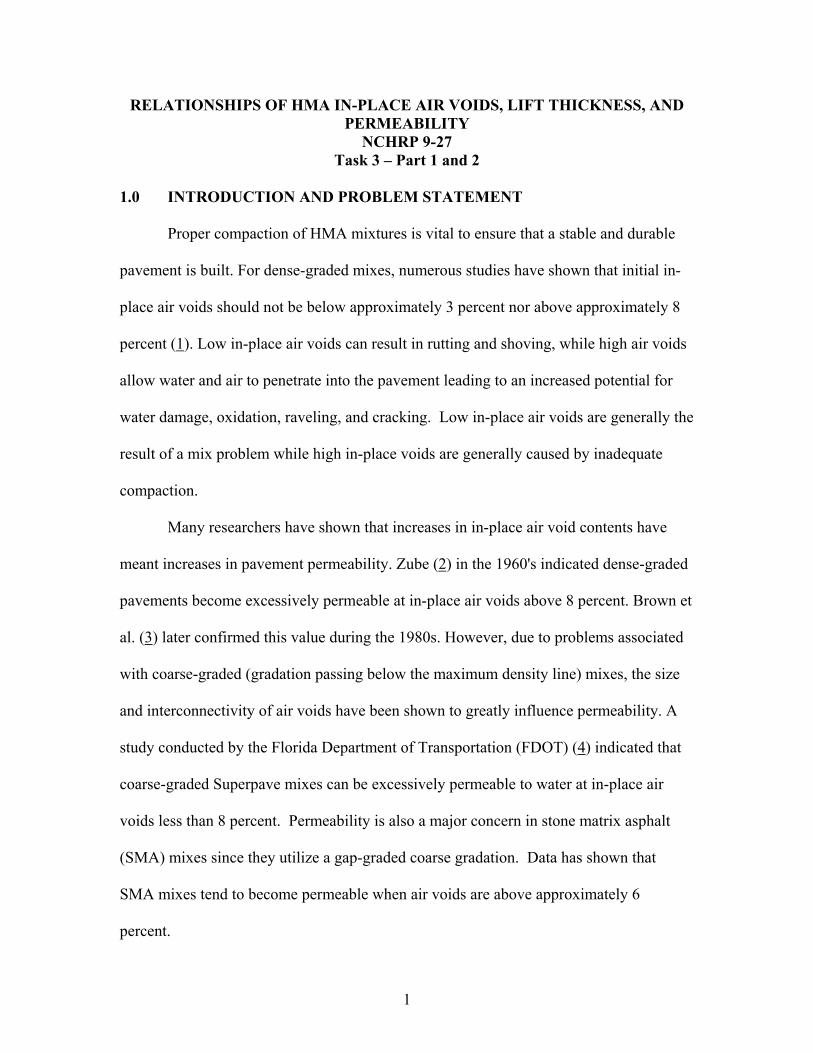
RELATIONSHIPS OF HMA IN-PLACE AIR VOIDS, LIFT THICKNESS, AND PERMEABILITY

NCHRP 9-27 Task 3 – Part 1 and 2

1.0 INTRODUCTION AND PROBLEM STATEMENT

Proper compaction of HMA mixtures is vital to ensure that a stable and durable

pavement is built. For dense-graded mixes, numerous studies have shown that initial in-

place air voids should not be below approximately 3 percent nor above approximately 8

percent (1). Low in-place air voids can result in rutting and shoving, while high air voids

allow water and air to penetrate into the pavement leading to an increased potential for

water damage, oxidation, raveling, and cracking. Low in-place air voids are generally the

result of a mix problem while high in-place voids are generally caused by inadequate

compaction.

Many researchers have shown that increases in in-place air void contents have

meant increases in pavement permeability. Zube (2) in the 1960's indicated dense-graded

pavements become excessively permeable at in-place air voids above 8 percent. Brown et

al. (3) later confirmed this value during the 1980s. However, due to problems associated

with coarse-graded (gradation passing below the maximum density line) mixes, the size

and interconnectivity of air voids have been shown to greatly influence permeability. A

study conducted by the Florida Department of Transportation (FDOT) (4) indicated that

coarse-graded Superpave mixes can be excessively permeable to water at in-place air

voids less than 8 percent. Permeability is also a major concern in stone matrix asphalt

(SMA) mixes since they utilize a gap-graded coarse gradation. Data has shown that

SMA mixes tend to become permeable when air voids are above approximately 6

percent.

2

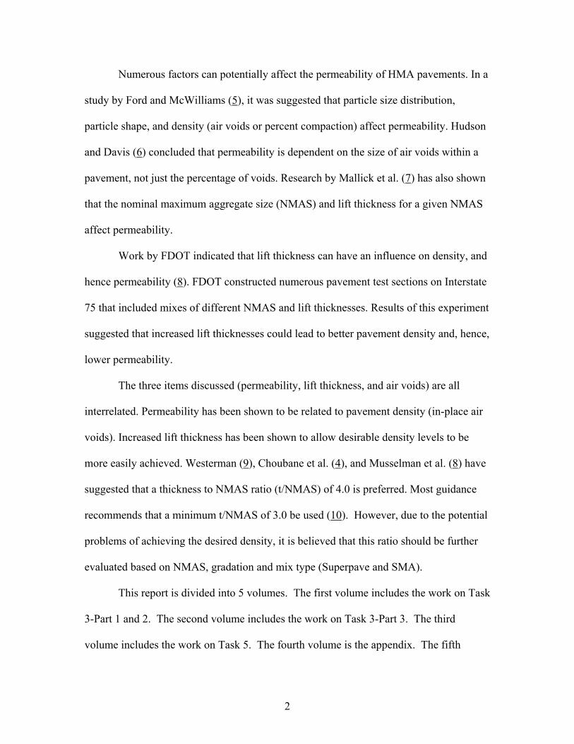
Numerous factors can potentially affect the permeability of HMA pavements. In a

study by Ford and McWilliams (5), it was suggested that particle size distribution,

particle shape, and density (air voids or percent compaction) affect permeability. Hudson

and Davis (6) concluded that permeability is dependent on the size of air voids within a

pavement, not just the percentage of voids. Research by Mallick et al. (7) has also shown

that the nominal maximum aggregate size (NMAS) and lift thickness for a given NMAS

affect permeability.

Work by FDOT indicated that lift thickness can have an influence on density, and

hence permeability (8). FDOT constructed numerous pavement test sections on Interstate

75 that included mixes of different NMAS and lift thicknesses. Results of this experiment

suggested that increased lift thicknesses could lead to better pavement density and, hence,

lower permeability.

The three items discussed (permeability, lift thickness, and air voids) are all

interrelated. Permeability has been shown to be related to pavement density (in-place air

voids). Increased lift thickness has been shown to allow desirable density levels to be

more easily achieved. Westerman (9), Choubane et al. (4), and Musselman et al. (8) have

suggested that a thickness to NMAS ratio (t/NMAS) of 4.0 is preferred. Most guidance

recommends that a minimum t/NMAS of 3.0 be used (10). However, due to the potential

problems of achieving the desired density, it is believed that this ratio should be further

evaluated based on NMAS, gradation and mix type (Superpave and SMA).

This report is divided into 5 volumes. The first volume includes the work on Task

3-Part 1 and 2. The second volume includes the work on Task 3-Part 3. The third

volume includes the work on Task 5. The fourth volume is the appendix. The fifth

3

volume is an executive summary of the work.

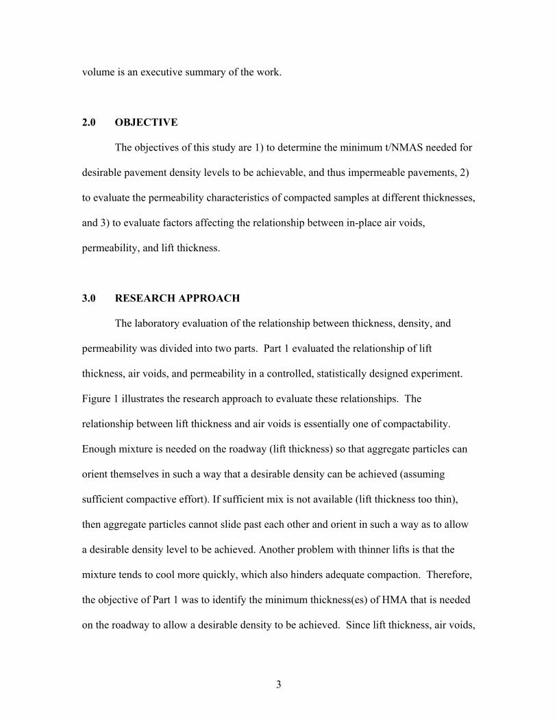
2.0 OBJECTIVE

The objectives of this study are 1) to determine the minimum t/NMAS needed for

desirable pavement density levels to be achievable, and thus impermeable pavements, 2)

to evaluate the permeability characteristics of compacted samples at different thicknesses,

and 3) to evaluate factors affecting the relationship between in-place air voids,

permeability, and lift thickness.

3.0 RESEARCH APPROACH

The laboratory evaluation of the relationship between thickness, density, and

permeability was divided into two parts. Part 1 evaluated the relationship of lift

thickness, air voids, and permeability in a controlled, statistically designed experiment.

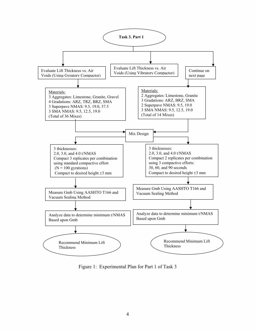
Figure 1 illustrates the research approach to evaluate these relationships. The

relationship between lift thickness and air voids is essentially one of compactability.

Enough mixture is needed on the roadway (lift thickness) so that aggregate particles can

orient themselves in such a way that a desirable density can be achieved (assuming

sufficient compactive effort). If sufficient mix is not available (lift thickness too thin),

then aggregate particles cannot slide past each other and orient in such a way as to allow

a desirable density level to be achieved. Another problem with thinner lifts is that the

mixture tends to cool more quickly, which also hinders adequate compaction. Therefore,

the objective of Part 1 was to identify the minimum thickness(es) of HMA that is needed

on the roadway to allow a desirable density to be achieved. Since lift thickness, air voids,

4

Figure 1: Experimental Plan for Part 1 of Task 3

Task 3, Part 1

Evaluate Lift Thickness vs. Air Voids (Using Vibratory Compactor)

Materials: 2 Aggregates: Limestone, Granite 3 Gradations: ARZ, BRZ, SMA 2 Superpave NMAS: 9.5, 19.0 3 SMA NMAS: 9.5, 12.5, 19.0 (Total of 14 Mixes)

3 thicknesses: 2.0, 3.0, and 4.0 t/NMAS Compact 2 replicates per combination using 3 compactive efforts: 30, 60, and 90 seconds Compact to desired height ±3 mm

Measure Gmb Using AASHTO T166 and Vacuum Sealing Method

Analyze data to determine minimum t/NMAS Based upon Gmb

Recommend Minimum Lift Thickness

Evaluate Lift Thickness vs. Air Voids (Using Gyratory Compactor)

Materials: 3 Aggregates: Limestone, Granite, Gravel 4 Gradations: ARZ, TRZ, BRZ, SMA 3 Superpave NMAS: 9.5, 19.0, 37.5 3 SMA NMAS: 9.5, 12.5, 19.0 (Total of 36 Mixes)

Mix Design

3 thicknesses: 2.0, 3.0, and 4.0 t/NMAS Compact 3 replicates per combination using standard compactive effort (N = 100 gyrations) Compact to desired height ±3 mm

Measure Gmb Using AASHTO T166 and Vacuum Sealing Method

Recommend Minimum Lift Thickness

Analyze data to determine minimum t/NMAS Based upon Gmb

Continue on next page

5

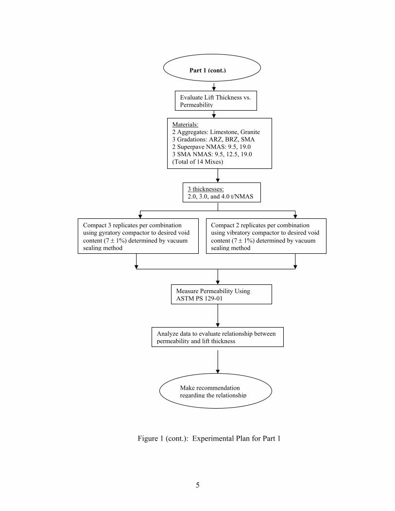
Figure 1 (cont.): Experimental Plan for Part 1

Part 1 (cont.)

Evaluate Lift Thickness vs. Permeability

Materials: 2 Aggregates: Limestone, Granite 3 Gradations: ARZ, BRZ, SMA 2 Superpave NMAS: 9.5, 19.0 3 SMA NMAS: 9.5, 12.5, 19.0 (Total of 14 Mixes)

3 thicknesses: 2.0, 3.0, and 4.0 t/NMAS

Compact 2 replicates per combination using vibratory compactor to desired void content (7 ± 1%) determined by vacuum sealing method

Measure Permeability Using ASTM PS 129-01

Analyze data to evaluate relationship between permeability and lift thickness

Make recommendation regarding the relationship

Compact 3 replicates per combination using gyratory compactor to desired void content (7 ± 1%) determined by vacuum sealing method

6

and permeability are interrelated; another objective was to investigate the permeability

characteristics of compacted HMA at different thicknesses.

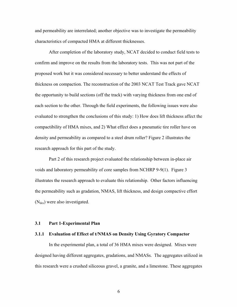
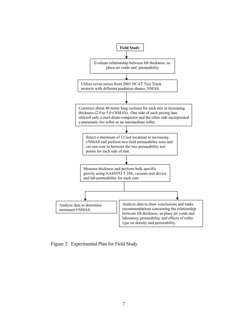
After completion of the laboratory study, NCAT decided to conduct field tests to

confirm and improve on the results from the laboratory tests. This was not part of the

proposed work but it was considered necessary to better understand the effects of

thickness on compaction. The reconstruction of the 2003 NCAT Test Track gave NCAT

the opportunity to build sections (off the track) with varying thickness from one end of

each section to the other. Through the field experiments, the following issues were also

evaluated to strengthen the conclusions of this study: 1) How does lift thickness affect the

compactibility of HMA mixes, and 2) What effect does a pneumatic tire roller have on

density and permeability as compared to a steel drum roller? Figure 2 illustrates the

research approach for this part of the study.

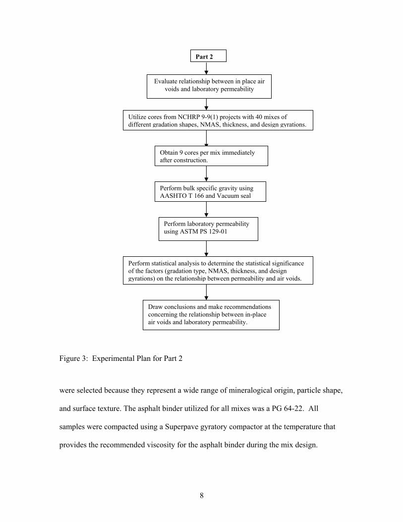
Part 2 of this research project evaluated the relationship between in-place air

voids and laboratory permeability of core samples from NCHRP 9-9(1). Figure 3

illustrates the research approach to evaluate this relationship. Other factors influencing

the permeability such as gradation, NMAS, lift thickness, and design compactive effort

(Ndes) were also investigated.

3.1 Part 1-Experimental Plan

3.1.1 Evaluation of Effect of t/NMAS on Density Using Gyratory Compactor

In the experimental plan, a total of 36 HMA mixes were designed. Mixes were

designed having different aggregates, gradations, and NMASs. The aggregates utilized in

this research were a crushed siliceous gravel, a granite, and a limestone. These aggregates

7

Figure 2: Experimental Plan for Field Study

Analyze data to draw conclusions and make recommendations concerning the relationship between lift thickness, in-place air voids and laboratory permeability and effects of roller type on density and permeability.

Analyze data to determine minimum t/NMAS

Evaluate relationship between lift thickness, in-place air voids and permeability

Utilize seven mixes from 2003 NCAT Test Track projects with different gradation shapes, NMAS.

Construct about 40 meter long sections for each mix at increasing thickness (2.0 to 5.0 t/NMAS). One side of each paving lane utilized only a steel drum compactor and the other side incorporated a pneumatic tire roller as an intermediate roller.

Measure thickness and perform bulk specific gravity using AASHTO T 166, vacuum seal device and lab permeability for each core

Field Study

Select a minimum of 12 test locations at increasing t/NMAS and perform two field permeability tests and cut one core in between the two permeability test points for each side of mat.

8

Figure 3: Experimental Plan for Part 2

were selected because they represent a wide range of mineralogical origin, particle shape,

and surface texture. The asphalt binder utilized for all mixes was a PG 64-22. All

samples were compacted using a Superpave gyratory compactor at the temperature that

provides the recommended viscosity for the asphalt binder during the mix design.

Draw conclusions and make recommendations concerning the relationship between in-place air voids and laboratory permeability.

Perform statistical analysis to determine the statistical significance of the factors (gradation type, NMAS, thickness, and design gyrations) on the relationship between permeability and air voids.

Perform laboratory permeability using ASTM PS 129-01

Evaluate relationship between in place air voids and laboratory permeability

Utilize cores from NCHRP 9-9(1) projects with 40 mixes of different gradation shapes, NMAS, thickness, and design gyrations.

Obtain 9 cores per mix immediately after construction.

Perform bulk specific gravity using AASHTO T 166 and Vacuum seal

Part 2

9

The experiment also included four gradation shapes and three nominal maximum

aggregate sizes (NMAS). Three gradations fell within Superpave gradation control points

and one gradation conformed to stone matrix asphalt specifications. For the gradations

meeting the Superpave requirements, NMASs of 9.5, 19.0 and 37.5 mm were

investigated. For the SMA gradations, NMASs of 9.5, 12.5, and 19.0 mm were utilized.

The three Superpave gradations included one gradation that passed near the upper

gradation control limits and above the restricted zone (ARZ), one that resided near the

maximum density line and passed through the restricted zone (TRZ), and one that passed

near the lower gradation control limits and below the restricted zone (BRZ). This

resulted in a total of 36 mix designs.

The property selected to define lift thickness in this experiment was the ratio of

thickness to NMAS (t/NMAS). This ratio was selected for two reasons: (1) the ratio

normalizes lift thickness for any type of gradation and (2) a general rule-of-thumb for

Superpave mixes has been a t/NMAS ratio of 3.0 be used during construction (10). For

each NMAS in the experiment, three t/NMAS ratios were investigated. For the 9.5 and

19.0 mm NMAS Superpave mixes and all three SMA NMASs (9.5, 12.5, and 19.0 mm),

t/NMAS ratios of 2.0, 3.0, and 4.0 were used. Additional ratios of 8.0 and 6.0 for 9.5 and

12.5 mm NMAS, respectively, were also evaluated to better define the relationship where

air voids reach a limiting value (approximately 4.0 percent air voids). For the 37.5 mm

NMAS Superpave mixes, ratios of 2.0, 2.5, and 3.0 were investigated. The 4.0 t/NMAS

was excluded for the 37.5 mm NMAS mixes since this ratio would produce a 150 mm (6

in.) lift thickness which is unlikely to be used in the field. The desired thicknesses of

samples (2.0, 2.5, 3.0, 4.0, 6.0 and 8.0 t/NMAS) were achieved by altering the mass

10

placed in the mold prior to compaction (as mass changes for a given compactive effort,

thickness will change). All samples were short-term aged prior to compaction according

to “Standard Practice for Mixture Conditioning of HMA”, AASHTO PP2-01. This

procedure simulates aging of mixture during production and placement.

Three replicates of each aggregate-gradation-NMAS-thickness combination were

compacted using a single Superpave gyratory compactor. For the Superpave mixes, each

sample was compacted to 100 gyrations, the upper limit that most state DOTs use. The

100-gyration level was selected because it is probably the compactive effort that presents

the most difficulty in obtaining adequate density. For the SMA mixes, each sample was

compacted to 75 gyrations in the Superpave gyratory compactor in accordance with the

“Standard Practice for Designing SMA”, AASHTO PP44-01. The reason for using 75

gyrations was that all the aggregate types had Los Angeles abrasion values of more than

30 percent. Cellulose fiber was used as the fiber within the SMA mixes at 0.3 percent of

total mass. Designs were conducted to determine the asphalt binder content necessary to

produce 4.0 percent air voids at the design number of gyrations. Testing of each sample

after compaction included measuring the bulk specific gravity of each replicate using

both AASHTO T166 and the vacuum sealing method. A standard test method has been

developed for the vacuum sealing method, ASTM D6752-02a, “Bulk Specific Gravity

and Density of Compacted Bituminous Mixtures Using Automatic Vacuum Sealing

Method.” A statistical analysis of the data was then conducted.

3.1.2 Evaluation of Effect of t/NMAS on Density Using Vibratory Compactor

To further evaluate the relationship between density and lift thickness, a similar

11

study was conducted but on a smaller scale, using the vibratory compactor as the

compaction mode. This was not part of the original proposed work but it was believed

that the vibratory compactor might provide compaction that has more typical of in-place

compaction. Of the 36 mix designs from Part 1, 14 mixes were selected for this study.

Two types of aggregates, granite and limestone were used. For Superpave designed

mixes, two gradations were utilized (ARZ and BRZ) along with two NMASs (9.5 mm

and 19.0 mm). The 37.5 mm NMAS mix was excluded from the study because the

maximum thickness of the vibratory specimen that could be obtained was 75.0 mm,

which would only be 2.0 t/NMAS. For the SMA mixes, three NMASs were selected (9.5

mm, 12.5 mm and 19 mm). The t/NMAS ratios utilized were 2.0, 3.0 and 4.0. The

compactive effort for each t/NMAS was varied over a range including 30 sec, 60 sec, and

90 sec of compaction. The range of compactive efforts was selected for two reasons: (1)

there is no standard compactive effort for the vibratory compactor and (2) the effects of

compactive effort on density at different thicknesses could be evaluated. After

compaction, the bulk specific gravity was measured and the data was analyzed to provide

recommendations concerning the minimum t/NMAS.

3.1.3 Evaluation of Effect of t/NMAS on Density Using Field Experiment

NCAT also conducted a field study to evaluate the acceptable minimum lift

thickness. Through the field experiments, the following issues were also evaluated to

strengthen the conclusions of this study: 1) How does lift thickness affect the

compactibility of HMA mixes, and 2) What effect does a pneumatic tire roller have on

density as compared to a steel drum roller?

12

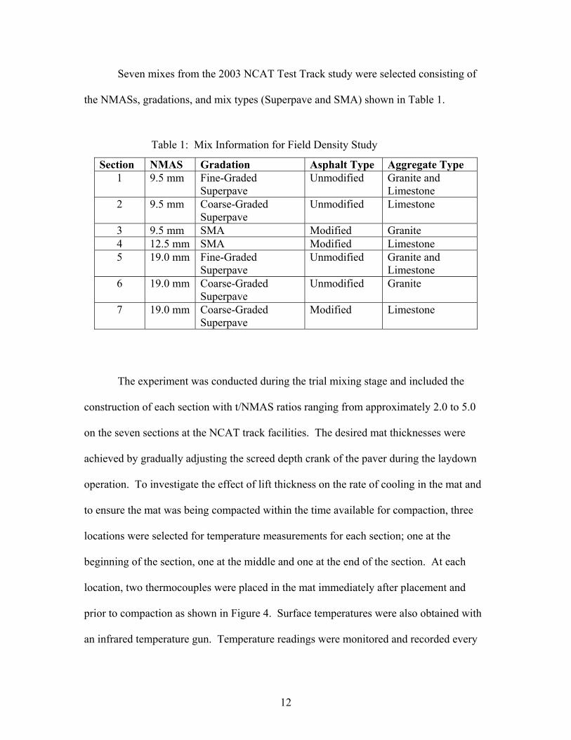
Seven mixes from the 2003 NCAT Test Track study were selected consisting of

the NMASs, gradations, and mix types (Superpave and SMA) shown in Table 1.

Table 1: Mix Information for Field Density Study

Section NMAS Gradation Asphalt Type Aggregate Type 1 9.5 mm Fine-Graded

Superpave Unmodified Granite and

Limestone 2 9.5 mm Coarse-Graded

Superpave Unmodified Limestone

3 9.5 mm SMA Modified Granite 4 12.5 mm SMA Modified Limestone 5 19.0 mm Fine-Graded

Superpave Unmodified Granite and

Limestone 6 19.0 mm Coarse-Graded

Superpave Unmodified Granite

7 19.0 mm Coarse-Graded Superpave

Modified Limestone

The experiment was conducted during the trial mixing stage and included the

construction of each section with t/NMAS ratios ranging from approximately 2.0 to 5.0

on the seven sections at the NCAT track facilities. The desired mat thicknesses were

achieved by gradually adjusting the screed depth crank of the paver during the laydown

operation. To investigate the effect of lift thickness on the rate of cooling in the mat and

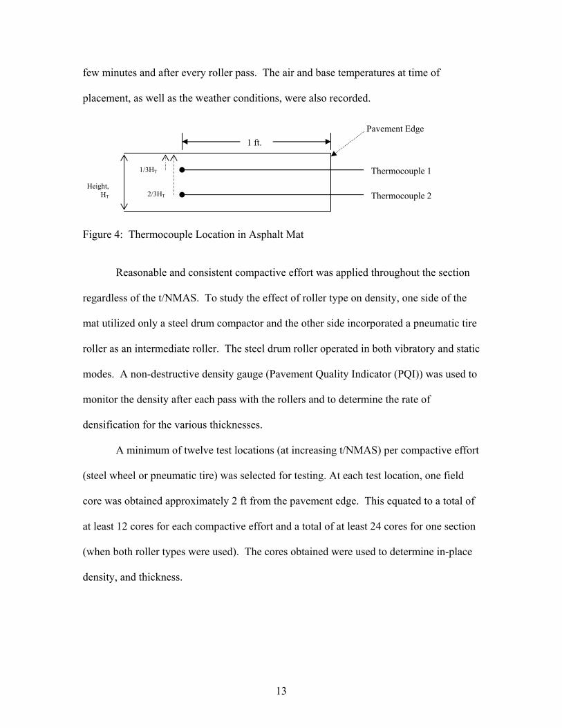
to ensure the mat was being compacted within the time available for compaction, three

locations were selected for temperature measurements for each section; one at the

beginning of the section, one at the middle and one at the end of the section. At each

location, two thermocouples were placed in the mat immediately after placement and

prior to compaction as shown in Figure 4. Surface temperatures were also obtained with

an infrared temperature gun. Temperature readings were monitored and recorded every

13

few minutes and after every roller pass. The air and base temperatures at time of

placement, as well as the weather conditions, were also recorded.

Figure 4: Thermocouple Location in Asphalt Mat

Reasonable and consistent compactive effort was applied throughout the section

regardless of the t/NMAS. To study the effect of roller type on density, one side of the

mat utilized only a steel drum compactor and the other side incorporated a pneumatic tire

roller as an intermediate roller. The steel drum roller operated in both vibratory and static

modes. A non-destructive density gauge (Pavement Quality Indicator (PQI)) was used to

monitor the density after each pass with the rollers and to determine the rate of

densification for the various thicknesses.

A minimum of twelve test locations (at increasing t/NMAS) per compactive effort

(steel wheel or pneumatic tire) was selected for testing. At each test location, one field

core was obtained approximately 2 ft from the pavement edge. This equated to a total of

at least 12 cores for each compactive effort and a total of at least 24 cores for one section

(when both roller types were used). The cores obtained were used to determine in-place

density, and thickness.

Height,HT

1 ft.Pavement Edge

Thermocouple 1

Thermocouple 2

1/3HT

2/3HT

14

3.1.4 Evaluation of Effect of Temperature on Relationship Between Density and

t/NMAS from Field Experiment

Recall from the field experiment that three locations were selected for

temperature measurements for each section; one near the beginning of the section, one

near the middle, and one near the end of section. This was done because the rate of

cooling varied from one end to the other due to change of thickness. The rate of cooling

was determined by plotting the average temperature from each location against time. To

determine the effect of temperature on the density, the temperature at 20 minutes after

placement of mix was selected. This number is somewhat arbitrary but it is realistic

because in general, the compaction in the field should be obtained within approximately

20 minutes after paving. Since the mixes in this study used two different types of asphalt

binder, (PG 67-22 and PG 76-22), the temperatures at 20 minutes were normalized by

subtracting the high temperature grade of the asphalt binder from the measured mat

temperatures at 20 minutes. For instance, if the temperature at 20 minutes was 100oC for

a mix using PG 67-22, the difference of the temperature was 33oC (100oC – 67oC). This

was done because in general the higher PG binder (PG 76-22) would require a higher

compaction temperature and hence it is the difference in the mix temperature and the high

temperature PG grade that affects compaction.

3.1.5 Evaluation of Effect of t/NMAS on Permeability Using Gyratory Compactor

To investigate the permeability characteristics of HMA at different thicknesses,

the same 14 mixes used in the experiment to determine the effect of t/NMAS on density

using vibratory compactor were utilized. The gyratory compactor height for t/NMAS

15

ratios of 2.0, 3.0, and 4.0 was determined and samples were compacted with appropriate

mass to produce 7.0 ± 1 percent air voids. The 7.0 percent air voids was selected to

simulate the density of a pavement in the field after construction. The bulk specific

gravity was measured using the vacuum seal method. Permeability tests were performed

on all samples and the relationships between permeability and lift thickness evaluated.

3.1.6 Evaluation of Effect of t/NMAS on Permeability Using Vibratory Compactor

For this study, the same 14 mixes used in the previous vibratory compactor study

were utilized. T/NMAS ratios of 2.0, 3.0, and 4.0 were used and two beams of each

aggregate-gradation-t/NMAS combination were compacted to 7.0 ± 1 percent air voids.

Two 100 mm cores were cut from the beams. Bulk specific gravity for beams and cores

was determined using the vacuum seal method. Permeability tests were performed on all

core samples and the relationships between permeability and lift thickness evaluated.

3.1.7 Evaluation of the Effect of t/NMAS on Permeability Using Field Experiment

The seven sections constructed to determine the minimum t/NMAS from the field

experiment were utilized in this study. The effect of roller type on permeability was also

evaluated. A minimum of twelve test locations per compactive effort (steel wheel or

pneumatic tire) was selected for testing. Two field permeability tests were performed at

the locations where the cores were obtained as shown in Figure 5. Laboratory

permeability testing was also performed on the cores obtained from each section. This

was done to evaluate the relationships between laboratory and field permeability tests.

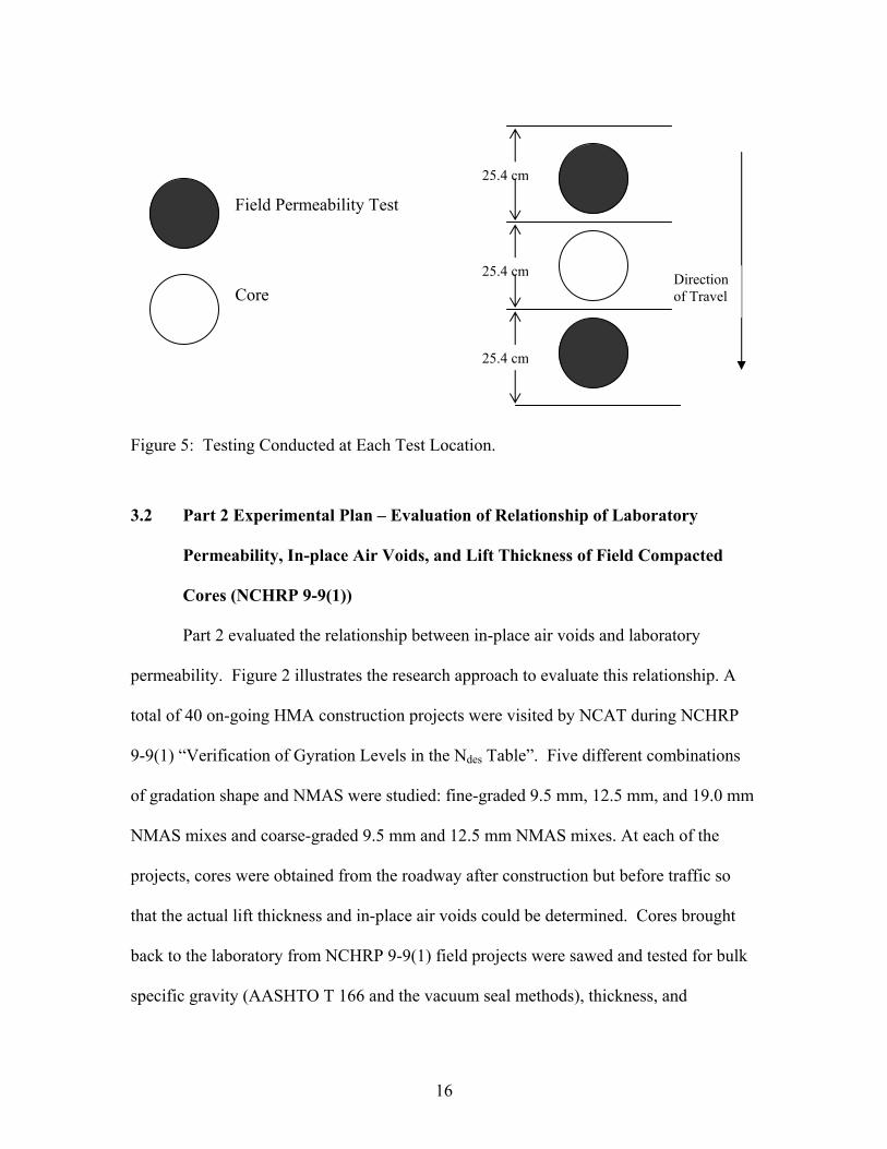
16

Field Permeability Test

Core

Figure 5: Testing Conducted at Each Test Location.

3.2 Part 2 Experimental Plan – Evaluation of Relationship of Laboratory

Permeability, In-place Air Voids, and Lift Thickness of Field Compacted

Cores (NCHRP 9-9(1))

Part 2 evaluated the relationship between in-place air voids and laboratory

permeability. Figure 2 illustrates the research approach to evaluate this relationship. A

total of 40 on-going HMA construction projects were visited by NCAT during NCHRP

9-9(1) “Verification of Gyration Levels in the Ndes Table”. Five different combinations

of gradation shape and NMAS were studied: fine-graded 9.5 mm, 12.5 mm, and 19.0 mm

NMAS mixes and coarse-graded 9.5 mm and 12.5 mm NMAS mixes. At each of the

projects, cores were obtained from the roadway after construction but before traffic so

that the actual lift thickness and in-place air voids could be determined. Cores brought

back to the laboratory from NCHRP 9-9(1) field projects were sawed and tested for bulk

specific gravity (AASHTO T 166 and the vacuum seal methods), thickness, and

Direction of Travel

25.4 cm

25.4 cm

25.4 cm

17

laboratory permeability (ASTM PS 129-01). Plant-produced mix was also sampled at

each project in order to determine the theoretical maximum density (TMD) and the

mixture gradation. The TMD test was performed according to AASHTO T209.

4.0 MATERIALS AND TEST METHODS

4.1 Aggregate and Binder Properties

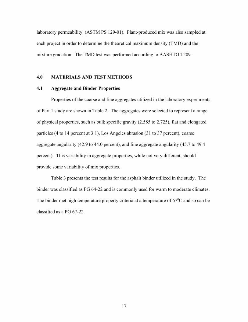
Properties of the coarse and fine aggregates utilized in the laboratory experiments

of Part 1 study are shown in Table 2. The aggregates were selected to represent a range

of physical properties, such as bulk specific gravity (2.585 to 2.725), flat and elongated

particles (4 to 14 percent at 3:1), Los Angeles abrasion (31 to 37 percent), coarse

aggregate angularity (42.9 to 44.0 percent), and fine aggregate angularity (45.7 to 49.4

percent). This variability in aggregate properties, while not very different, should

provide some variability of mix properties.

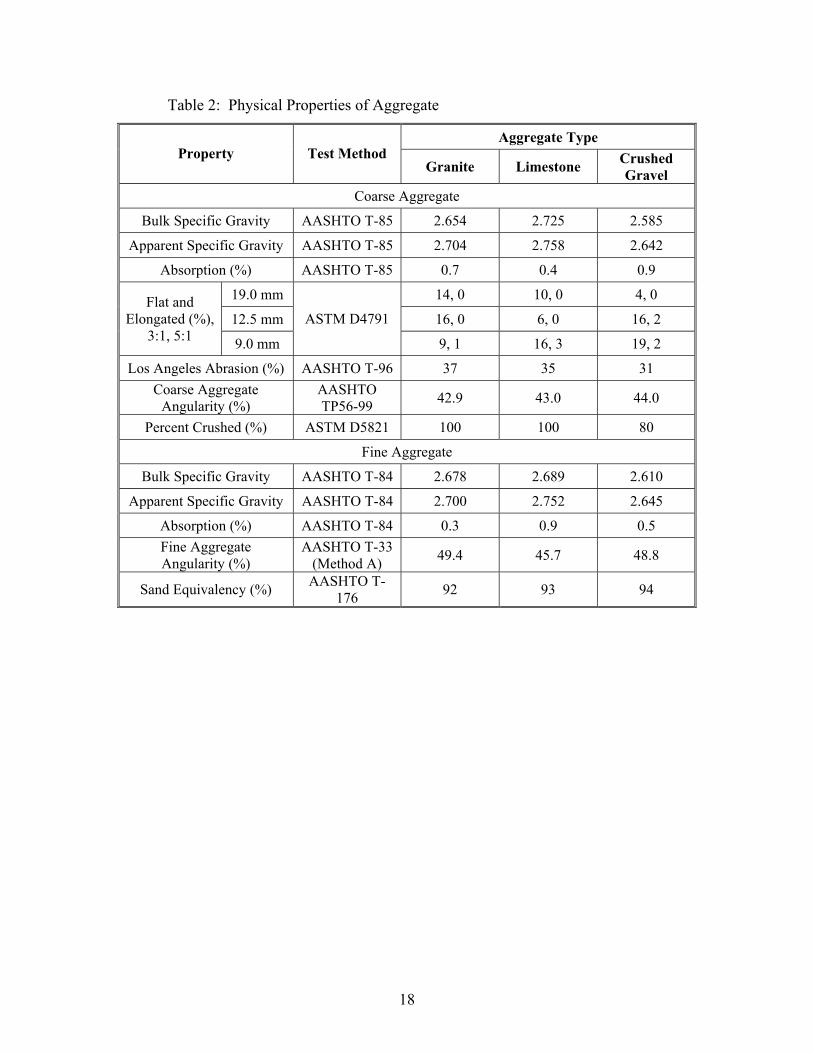
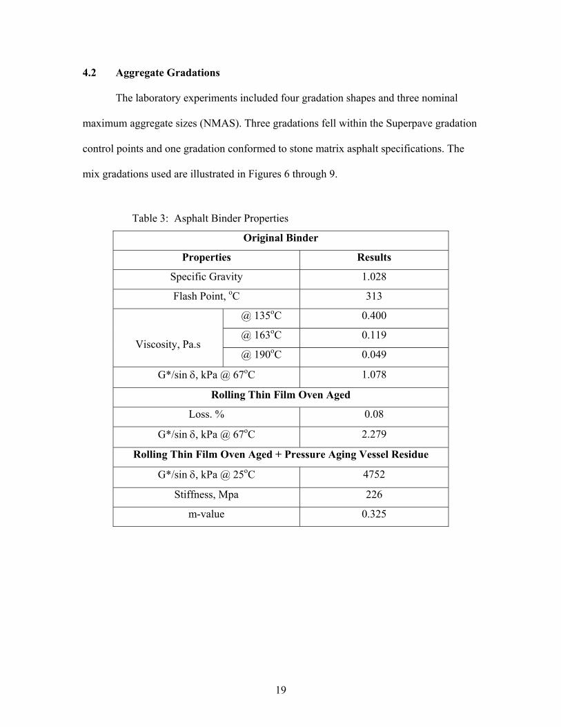
Table 3 presents the test results for the asphalt binder utilized in the study. The

binder was classified as PG 64-22 and is commonly used for warm to moderate climates.

The binder met high temperature property criteria at a temperature of 67oC and so can be

classified as a PG 67-22.

18

Table 2: Physical Properties of Aggregate

Aggregate Type Property Test Method

Granite Limestone Crushed Gravel

Coarse Aggregate

Bulk Specific Gravity AASHTO T-85 2.654 2.725 2.585

Apparent Specific Gravity AASHTO T-85 2.704 2.758 2.642

Absorption (%) AASHTO T-85 0.7 0.4 0.9

19.0 mm 14, 0 10, 0 4, 0

12.5 mm 16, 0 6, 0 16, 2 Flat and

Elongated (%), 3:1, 5:1 9.0 mm

ASTM D4791

9, 1 16, 3 19, 2

Los Angeles Abrasion (%) AASHTO T-96 37 35 31 Coarse Aggregate

Angularity (%) AASHTO TP56-99 42.9 43.0 44.0

Percent Crushed (%) ASTM D5821 100 100 80

Fine Aggregate

Bulk Specific Gravity AASHTO T-84 2.678 2.689 2.610

Apparent Specific Gravity AASHTO T-84 2.700 2.752 2.645

Absorption (%) AASHTO T-84 0.3 0.9 0.5 Fine Aggregate Angularity (%)

AASHTO T-33 (Method A) 49.4 45.7 48.8

Sand Equivalency (%) AASHTO T-176 92 93 94

19

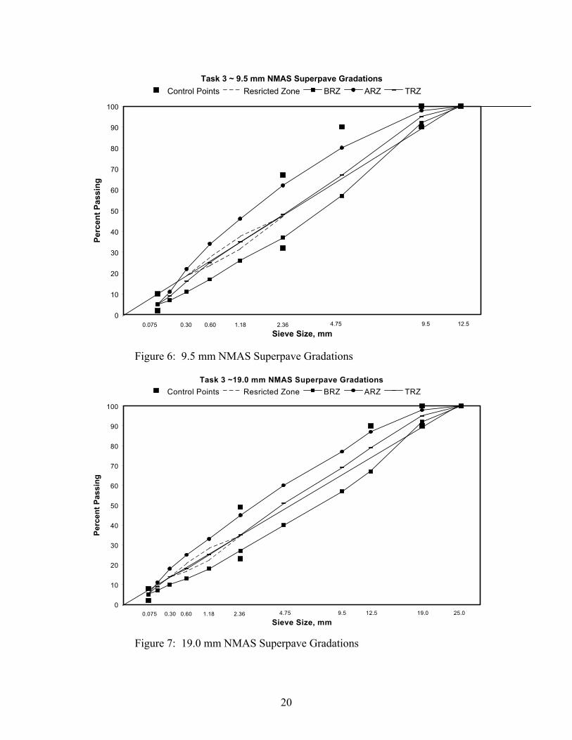
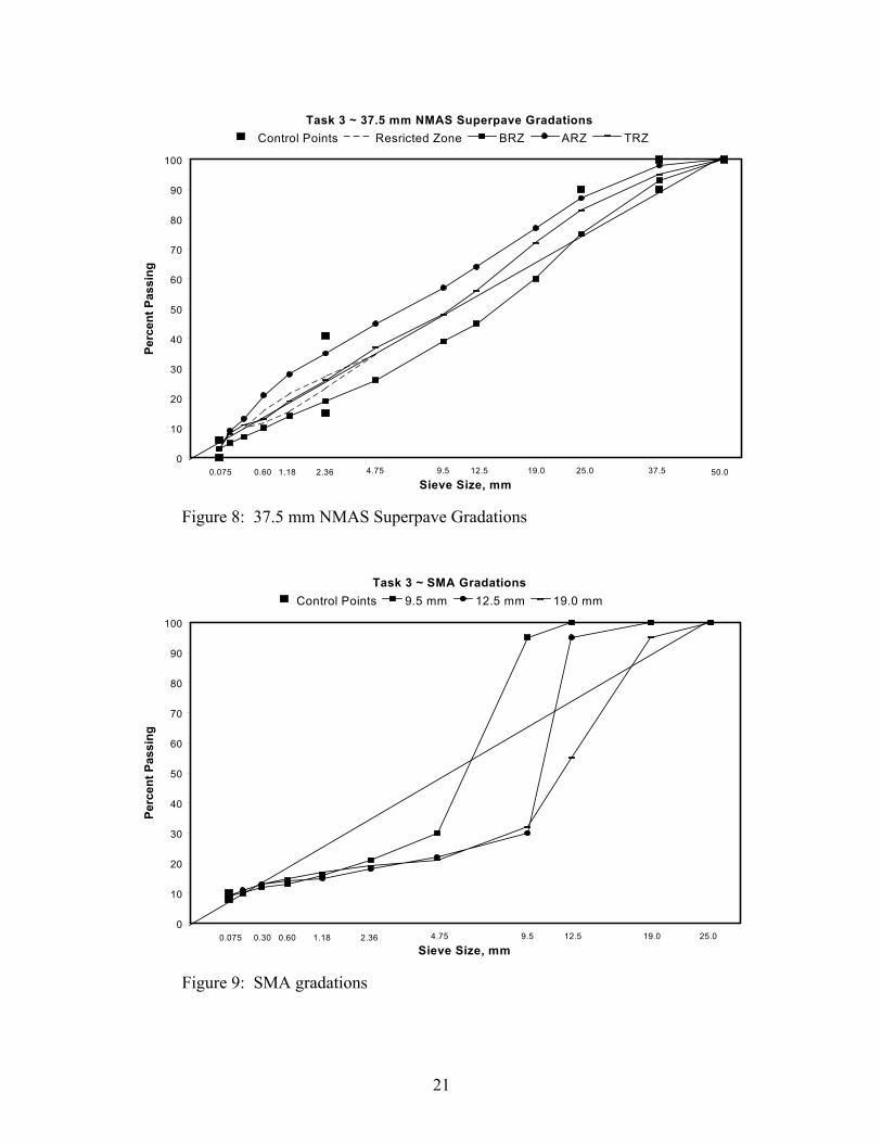
4.2 Aggregate Gradations

The laboratory experiments included four gradation shapes and three nominal

maximum aggregate sizes (NMAS). Three gradations fell within the Superpave gradation

control points and one gradation conformed to stone matrix asphalt specifications. The

mix gradations used are illustrated in Figures 6 through 9.

Table 3: Asphalt Binder Properties

Original Binder

Properties Results

Specific Gravity 1.028

Flash Point, oC 313

@ 135oC 0.400

@ 163oC 0.119

Viscosity, Pa.s @ 190oC 0.049

G*/sin δ, kPa @ 67oC 1.078

Rolling Thin Film Oven Aged

Loss. % 0.08

G*/sin δ, kPa @ 67oC 2.279

Rolling Thin Film Oven Aged + Pressure Aging Vessel Residue

G*/sin δ, kPa @ 25oC 4752

Stiffness, Mpa 226

m-value 0.325

20

Task 3 ~ 9.5 mm NMAS Superpave Gradations

0

10

20

30

40

50

60

70

80

90

100

Sieve Size, mm

Perc

ent P

assi

ngControl Points Resricted Zone BRZ ARZ TRZ

0.075 0.30 0.60 1.18 2.36 4.75 9.5 12.5

Figure 6: 9.5 mm NMAS Superpave Gradations

Task 3 ~19.0 mm NMAS Superpave Gradations

0

10

20

30

40

50

60

70

80

90

100

Sieve Size, mm

Perc

ent P

assi

ng

Control Points Resricted Zone BRZ ARZ TRZ

0.075 0.30 0.60 1.18 2.36 4.75 9.5 12.5 19.0 25.0


21

Task 3 ~ 37.5 mm NMAS Superpave Gradations

0

10

20

30

40

50

60

70

80

90

100

Sieve Size, mm

Perc

ent P

assi

ngControl Points Resricted Zone BRZ ARZ TRZ

0.075 0.60 1.18 2.36 4.75 9.5 12.5 19.0 25.0 50.037.5


Task 3 ~ SMA Gradations

0

10

20

30

40

50

60

70

80

90

100

Sieve Size, mm

Perc

ent P

assi

ng

Control Points 9.5 mm 12.5 mm 19.0 mm

0.075 0.30 0.60 1.18 2.36 4.75 9.5 12.5 19.0 25.0

Figure 9: SMA gradations

22

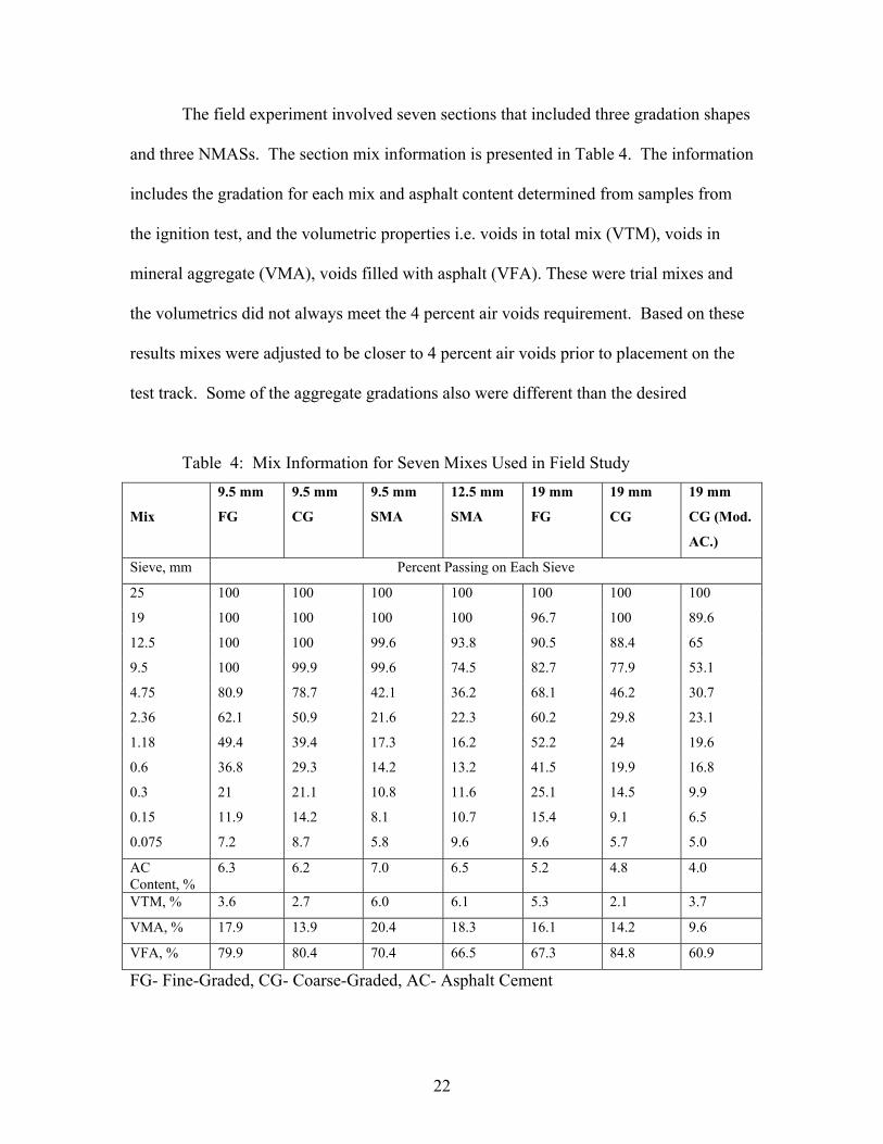
The field experiment involved seven sections that included three gradation shapes

and three NMASs. The section mix information is presented in Table 4. The information

includes the gradation for each mix and asphalt content determined from samples from

the ignition test, and the volumetric properties i.e. voids in total mix (VTM), voids in

mineral aggregate (VMA), voids filled with asphalt (VFA). These were trial mixes and

the volumetrics did not always meet the 4 percent air voids requirement. Based on these

results mixes were adjusted to be closer to 4 percent air voids prior to placement on the

test track. Some of the aggregate gradations also were different than the desired

Table 4: Mix Information for Seven Mixes Used in Field Study

Mix

9.5 mm

FG

9.5 mm

CG

9.5 mm

SMA

12.5 mm

SMA

19 mm

FG

19 mm

CG

19 mm

CG (Mod.

AC.)

Sieve, mm Percent Passing on Each Sieve

25 100 100 100 100 100 100 100

19 100 100 100 100 96.7 100 89.6

12.5 100 100 99.6 93.8 90.5 88.4 65

9.5 100 99.9 99.6 74.5 82.7 77.9 53.1

4.75 80.9 78.7 42.1 36.2 68.1 46.2 30.7

2.36 62.1 50.9 21.6 22.3 60.2 29.8 23.1

1.18 49.4 39.4 17.3 16.2 52.2 24 19.6

0.6 36.8 29.3 14.2 13.2 41.5 19.9 16.8

0.3 21 21.1 10.8 11.6 25.1 14.5 9.9

0.15 11.9 14.2 8.1 10.7 15.4 9.1 6.5

0.075 7.2 8.7 5.8 9.6 9.6 5.7 5.0

AC Content, %

6.3 6.2 7.0 6.5 5.2 4.8 4.0

VTM, % 3.6 2.7 6.0 6.1 5.3 2.1 3.7

VMA, % 17.9 13.9 20.4 18.3 16.1 14.2 9.6

VFA, % 79.9 80.4 70.4 66.5 67.3 84.8 60.9

FG- Fine-Graded, CG- Coarse-Graded, AC- Asphalt Cement

23

gradation, however, it was believed that this wide range of mix types would give a good

overall measure of the effect of t/NMAS on density and permeability.

4.3 Determination of Bulk Specific Gravity

The bulk specific gravity of all compacted samples was measured using both

AASHTO T166 and vacuum seal device. For AASHTO T166, Method A was utilized.

This consists of weighing a dry sample in air, then obtaining a submerged mass after the

sample has been placed in a water bath for 4 ± 1 minutes. Upon removal from the water

bath, the SSD mass is determined after blotting the sample dry as quickly as possible

using a damp towel.

The vacuum seal method was performed in accordance with ASTM D 6752 – 02a,

“Standard Test Method for Bulk Specific Gravity and Density of Compacted Bituminous

Mixtures Using Automatic Vacuum Sealing Method”. It consists of a vacuum-sealing

device utilizing an automatic vacuum chamber with a specially designed, puncture

resistant plastic bag, which tightly conforms to the sides of the sample and prevents water

from infiltrating into the sample. The procedure involved in sealing and analyzing the

compacted sample was as follows:

Step 1: Determine the density of the plastic bag (generally manufacturer provided).

Step 2: Place the compacted sample into the bag.

Step 3: Place the bag containing the sample inside the vacuum chamber.

Step 4: Close the vacuum chamber door. The vacuum pump starts automatically

and evacuates the chamber.

Step 5: In approximately two minutes, the chamber door automatically opens with

24

the sample completely sealed within the plastic bag and ready for water

displacement testing.

Step 6: Perform water displacement method. Correct the results for the bag density

and the displaced bag volume.

4.4 Determination of Permeability

Laboratory permeability tests were conducted in accordance with ASTM PS 129-01,

Standard Provisional Test Method for Measurement of Permeability of Bituminous

Paving Mixtures Using a Flexible Wall Permeameter. This method utilizes a falling head

approach for measuring permeability. Each core was vacuum-saturated for five minutes

prior to testing. Water from a graduated standpipe was allowed to flow through the

saturated sample and the time to reach a known change in head recorded. Saturation was

considered sufficient when the variation between four consecutive time interval

measurements was relatively small; in this case all within 10% of the mean. Darcy’s Law

is then applied to estimate permeability of the sample.

The field permeability testing was performed using the NCAT Field Permeameter.

This device has been shown to compare reasonably well with laboratory permeability

tests and produce a reasonable relationship with in-place air voids in a pavement.

4.5 Part 2 – Evaluation of Relationship of Laboratory Permeability, Density and

Lift Thickness of Field Compacted Cores

Of the 40 different Superpave projects visited during NCHRP 9-9(1), three

projects were omitted for the purpose of this study due to damaged samples. A total of

25

287 usable cores were obtained from the 37 projects. All cores were cut from the

roadway prior to traffic. Information about the projects is presented in Table 5. Of the

37 projects, 11 projects utilized a 9.5 mm NMAS gradation, 23 projects utilized a 12.5

mm NMAS gradation, and 3 projects utilized a 19.0 mm NMAS gradation. Gradations

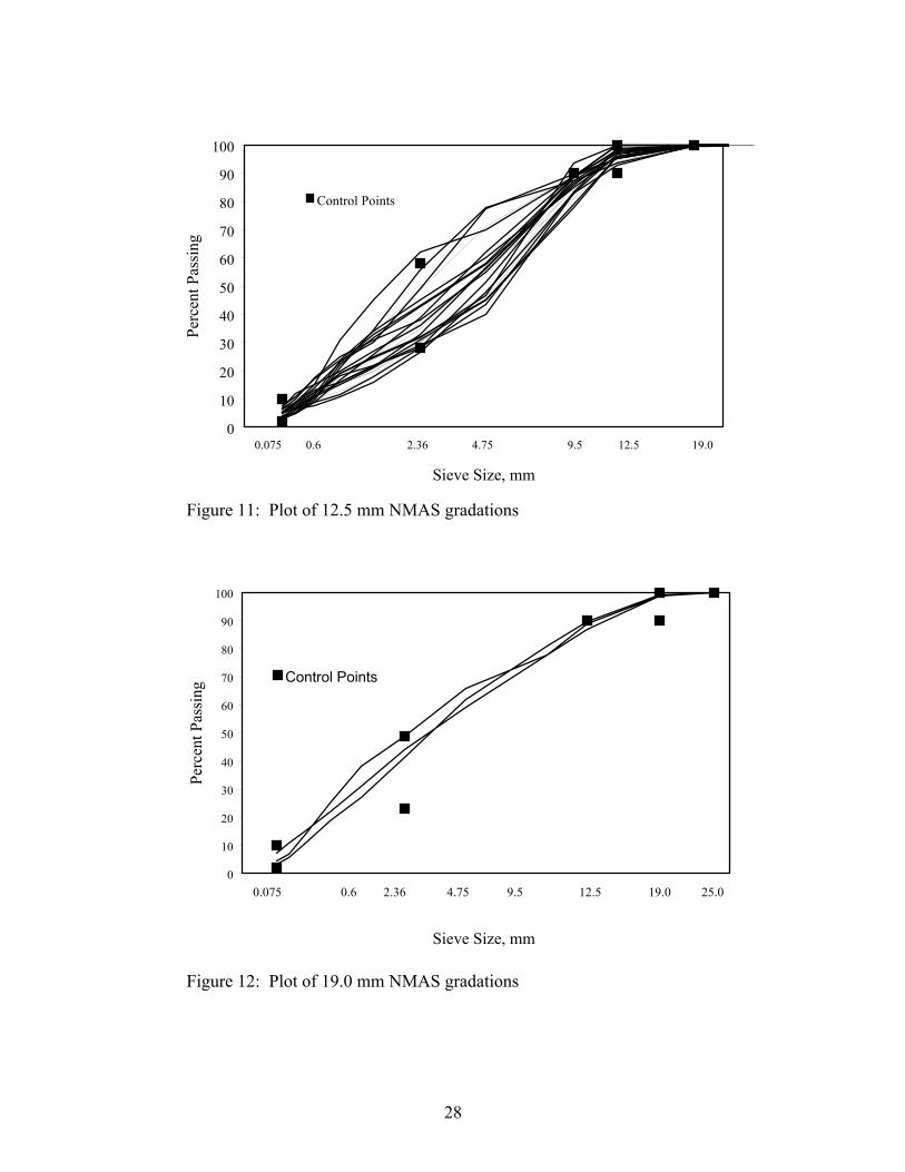
for all the mixes are illustrated in Figures 10 through 12, by NMAS from 9.5 to 19.0 mm,

respectively. For the purposes of this report, projects were identified as fine-graded or

coarse-graded according to the definition given by National Asphalt Pavement

Association (NAPA)(11). Percent passing certain sieve sizes for a given NMAS is used

to define fine- and coarse-graded mixes as shown in Table 6. Average lift thicknesses for

the different projects ranged from 22.3 to 78.8 mm and the Ndes ranged from 50 to 125

gyrations with a Superpave gyratory compactor.

5.0 TEST RESULTS AND ANALYSIS

5.1 Part 1 - Mix Designs

Of the 36 mix designs, 27 were Superpave designed mixes and 9 were SMA

mixes. The optimum asphalt content, the effective asphalt content (Pbe), voids in mineral

aggregate (VMA), voids filled with asphalt (VFA), percent theoretical maximum density

at Ninitial (% Gmm at Nini), ratio of dust to effective asphalt content (P0.075/Pbe) for the

Superpave mixtures summarized in Table 7; data for SMA mixes is shown in Table 8.

The mix design information for both mix types is presented in Appendix A. Optimum

asphalt binder content was chosen to provide 4 percent air voids at the design number of

gyrations. However, for the 19 mm NMAS limestone SMA mix 4 percent air voids could

be achieved with 5.7 percent asphalt content which did not meet the minimum asphalt

26

Table 5: Project Mix Information

Project NMAS, Gradation Asphalt Ndes Average No. (mm) Performance Thickness,

Grade (mm)

1 9.5 Coarse 67 - 22 86 34.3 2 9.5 Coarse 70 - 22 90 40.5 3 9.5 Coarse 70 - 22 90 44.5 4 9.5 Coarse 70 - 22 105 45.7 5 9.5 Coarse 64 - 22 50 31.2 6 9.5 Coarse 76 - 22 100 33.9 7 9.5 Coarse 58 - 22 125 34.9 8 9.5 Coarse 64 - 22 100 44.1 9 9.5 Coarse 70 - 28 100 22.3

10 9.5 Fine 58 - 28 75 40.5 11 9.5 Fine 58 - 28 75 32.4 12 12.5 Coarse 67 - 22 106 39.9 13 12.5 Coarse 67 - 22 100 42.4 14 12.5 Coarse 76 - 22 100 38.0 15 12.5 Coarse 67 - 22 75 33.7 16 12.5 Coarse 76 - 22 125 53.5 17 12.5 Coarse 76 - 22 125 51.0 18 12.5 Coarse 76 - 22 125 52.8 19 12.5 Coarse 76 – 22 125 56.8 20 12.5 Coarse 76 – 28 109 50.6 21 12.5 Coarse 64 – 28 86 47.6 22 12.5 Coarse 76 – 22 100 44.1 23 12.5 Coarse 70 – 22 125 51.1 24 12.5 Coarse 64 – 22 100 78.8 25 12.5 Coarse 70 – 22 125 48.4 26 12.5 Coarse 70 – 28 100 36.3 27 12.5 Fine 64 – 28 86 53.3 28 12.5 Fine 64 – 28 86 44.3 29 12.5 Fine 76 – 22 125 45.8 30 12.5 Fine 64 – 22 68 39.8 31 12.5 Fine 64 – 22 76 51.2 32 12.5 Fine 70 – 28 109 55.2 33 12.5 Fine 70 – 22 100 34.8 34 12.5 Fine 64 – 34 75 38.7 35 19 Fine 67 - 22 95 33.0 36 19 Fine 58 - 28 68 49.6 37 19 Fine 64 - 22 96 48.7

27

Table 6: Definition of Fine-and Coarse-Graded Mixes (11)

Mixture NMAS Coarse-Graded Fine-Graded

37.5 mm (1 ½”) <35 % Passing 4.75 mm

Sieve

>35 % Passing 4.75 mm

Sieve

25.0 mm (1”) <40 % Passing 4.75 mm

Sieve


Sieve

19.0 mm (3/4”) <35 % Passing 2.36 mm

Sieve


Sieve

12.5 mm (1/2”) <40 % Passing 2.36 mm

Sieve


Sieve

9.5 mm (3/8”) <45 % Passing 2.36 mm

Sieve


Sieve

4.75 mm (No. 4 Sieve) N/A (No standard Superpave gradation)

0

10

20

30

40

50

60

70

80

90

100

Sieve Size, mm

Per

cent

Pas

sing

Control Points

12.59.54.752.360.075

Figure 10: Plot of 9.5 mm NMAS gradations

28

0

10

20

30

40

50

60

70

80

90

100

Sieve Size, mm

Perc

ent P

assi

ngControl Points

0.075 2.36 4.75 9.5 12.5 19.00.6


0

10

20

30

40

50

60

70

80

90

100

Sieve Size, mm

Perc

ent P

assi

ng

Control Points

0.075 2.36 4.75 9.5 12.5 19.0 25.00.6


29

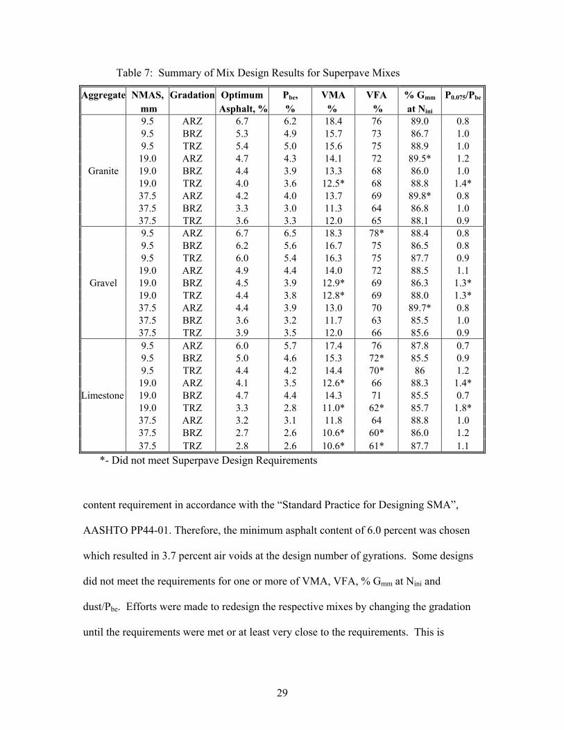
Table 7: Summary of Mix Design Results for Superpave Mixes

Aggregate NMAS, Gradation Optimum Pbe, VMA VFA % Gmm P0.075/Pbe

mm Asphalt, % % % % at Nini 9.5 ARZ 6.7 6.2 18.4 76 89.0 0.8 9.5 BRZ 5.3 4.9 15.7 73 86.7 1.0 9.5 TRZ 5.4 5.0 15.6 75 88.9 1.0 19.0 ARZ 4.7 4.3 14.1 72 89.5* 1.2

Granite 19.0 BRZ 4.4 3.9 13.3 68 86.0 1.0 19.0 TRZ 4.0 3.6 12.5* 68 88.8 1.4* 37.5 ARZ 4.2 4.0 13.7 69 89.8* 0.8 37.5 BRZ 3.3 3.0 11.3 64 86.8 1.0 37.5 TRZ 3.6 3.3 12.0 65 88.1 0.9

9.5 ARZ 6.7 6.5 18.3 78* 88.4 0.8 9.5 BRZ 6.2 5.6 16.7 75 86.5 0.8 9.5 TRZ 6.0 5.4 16.3 75 87.7 0.9 19.0 ARZ 4.9 4.4 14.0 72 88.5 1.1

Gravel 19.0 BRZ 4.5 3.9 12.9* 69 86.3 1.3* 19.0 TRZ 4.4 3.8 12.8* 69 88.0 1.3* 37.5 ARZ 4.4 3.9 13.0 70 89.7* 0.8 37.5 BRZ 3.6 3.2 11.7 63 85.5 1.0 37.5 TRZ 3.9 3.5 12.0 66 85.6 0.9 9.5 ARZ 6.0 5.7 17.4 76 87.8 0.7 9.5 BRZ 5.0 4.6 15.3 72* 85.5 0.9 9.5 TRZ 4.4 4.2 14.4 70* 86 1.2 19.0 ARZ 4.1 3.5 12.6* 66 88.3 1.4* Limestone 19.0 BRZ 4.7 4.4 14.3 71 85.5 0.7 19.0 TRZ 3.3 2.8 11.0* 62* 85.7 1.8* 37.5 ARZ 3.2 3.1 11.8 64 88.8 1.0 37.5 BRZ 2.7 2.6 10.6* 60* 86.0 1.2 37.5 TRZ 2.8 2.6 10.6* 61* 87.7 1.1

*- Did not meet Superpave Design Requirements

content requirement in accordance with the “Standard Practice for Designing SMA”,

AASHTO PP44-01. Therefore, the minimum asphalt content of 6.0 percent was chosen

which resulted in 3.7 percent air voids at the design number of gyrations. Some designs

did not meet the requirements for one or more of VMA, VFA, % Gmm at Nini and

dust/Pbe. Efforts were made to redesign the respective mixes by changing the gradation

until the requirements were met or at least very close to the requirements. This is

30

important in that the mixes used in this project were intended to duplicate mixes utilized

in the field. The adjusted gradations are presented in Tables 9 to 11. However, no

modification was made for the TRZ mixes that did not meet the requirements because

little could be done to modify gradations and still maintain the gradations passing through

the restricted zone.

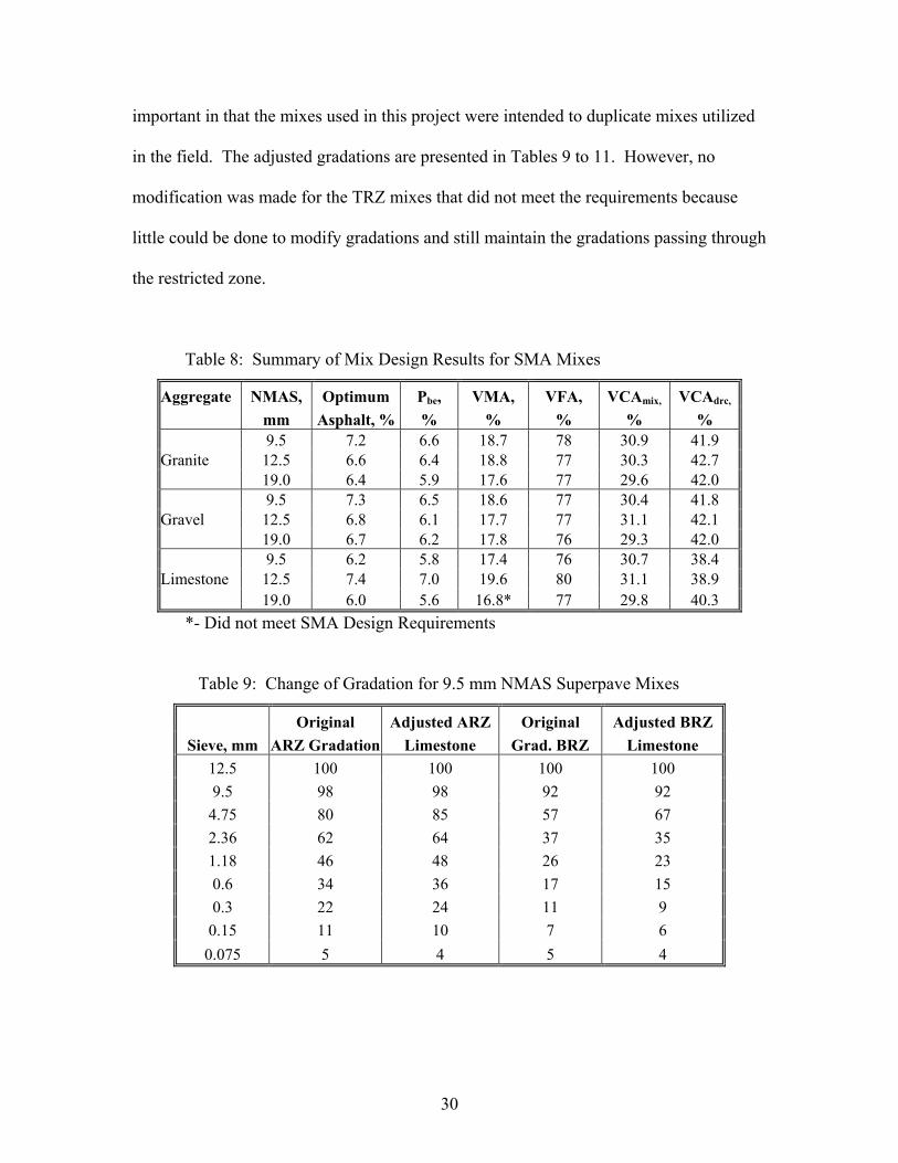
Table 8: Summary of Mix Design Results for SMA Mixes

Aggregate NMAS, Optimum Pbe, VMA, VFA, VCAmix, VCAdrc,

mm Asphalt, % % % % % % 9.5 7.2 6.6 18.7 78 30.9 41.9 Granite 12.5 6.6 6.4 18.8 77 30.3 42.7 19.0 6.4 5.9 17.6 77 29.6 42.0 9.5 7.3 6.5 18.6 77 30.4 41.8 Gravel 12.5 6.8 6.1 17.7 77 31.1 42.1 19.0 6.7 6.2 17.8 76 29.3 42.0 9.5 6.2 5.8 17.4 76 30.7 38.4 Limestone 12.5 7.4 7.0 19.6 80 31.1 38.9 19.0 6.0 5.6 16.8* 77 29.8 40.3

*- Did not meet SMA Design Requirements

Table 9: Change of Gradation for 9.5 mm NMAS Superpave Mixes

Original Adjusted ARZ Original Adjusted BRZ Sieve, mm ARZ Gradation Limestone Grad. BRZ Limestone

12.5 100 100 100 100 9.5 98 98 92 92

4.75 80 85 57 67 2.36 62 64 37 35 1.18 46 48 26 23 0.6 34 36 17 15 0.3 22 24 11 9

0.15 11 10 7 6 0.075 5 4 5 4

31

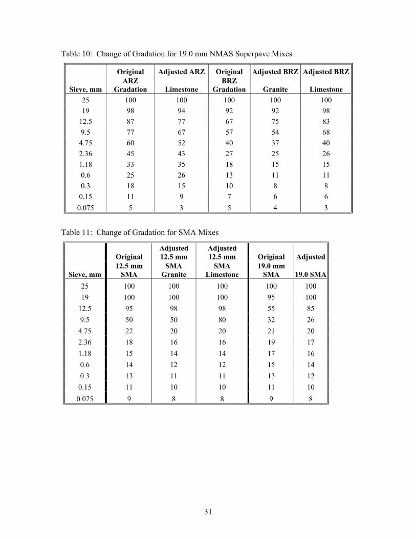
Table 10: Change of Gradation for 19.0 mm NMAS Superpave Mixes

Original Adjusted ARZ Original Adjusted BRZ Adjusted BRZ

Sieve, mm ARZ

Gradation Limestone BRZ

Gradation Granite Limestone 25 100 100 100 100 100 19 98 94 92 92 98

12.5 87 77 67 75 83 9.5 77 67 57 54 68

4.75 60 52 40 37 40 2.36 45 43 27 25 26 1.18 33 35 18 15 15 0.6 25 26 13 11 11 0.3 18 15 10 8 8

0.15 11 9 7 6 6 0.075 5 3 5 4 3

Table 11: Change of Gradation for SMA Mixes

Original Adjusted 12.5 mm

Adjusted 12.5 mm Original Adjusted

Sieve, mm 12.5 mm

SMA SMA

Granite SMA

Limestone 19.0 mm

SMA 19.0 SMA 25 100 100 100 100 100 19 100 100 100 95 100

12.5 95 98 98 55 85 9.5 50 50 80 32 26

4.75 22 20 20 21 20 2.36 18 16 16 19 17 1.18 15 14 14 17 16 0.6 14 12 12 15 14 0.3 13 11 11 13 12

0.15 11 10 10 11 10 0.075 9 8 8 9 8

32

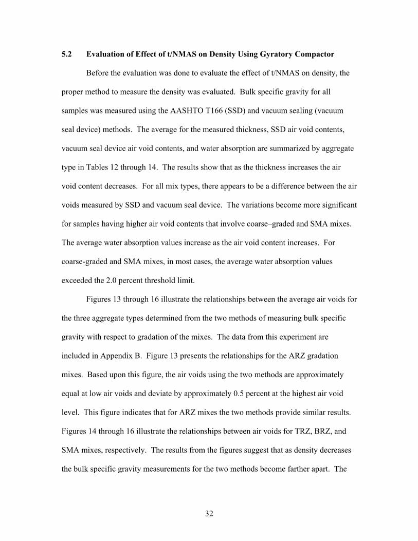
5.2 Evaluation of Effect of t/NMAS on Density Using Gyratory Compactor

Before the evaluation was done to evaluate the effect of t/NMAS on density, the

proper method to measure the density was evaluated. Bulk specific gravity for all

samples was measured using the AASHTO T166 (SSD) and vacuum sealing (vacuum

seal device) methods. The average for the measured thickness, SSD air void contents,

vacuum seal device air void contents, and water absorption are summarized by aggregate

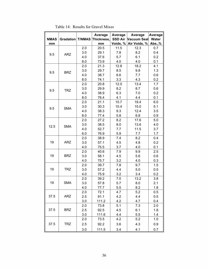
type in Tables 12 through 14. The results show that as the thickness increases the air

void content decreases. For all mix types, there appears to be a difference between the air

voids measured by SSD and vacuum seal device. The variations become more significant

for samples having higher air void contents that involve coarse–graded and SMA mixes.

The average water absorption values increase as the air void content increases. For

coarse-graded and SMA mixes, in most cases, the average water absorption values

exceeded the 2.0 percent threshold limit.

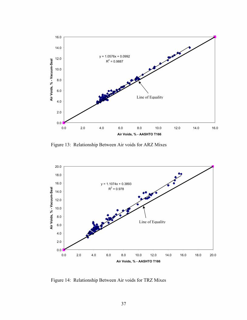
Figures 13 through 16 illustrate the relationships between the average air voids for

the three aggregate types determined from the two methods of measuring bulk specific

gravity with respect to gradation of the mixes. The data from this experiment are

included in Appendix B. Figure 13 presents the relationships for the ARZ gradation

mixes. Based upon this figure, the air voids using the two methods are approximately

equal at low air voids and deviate by approximately 0.5 percent at the highest air void

level. This figure indicates that for ARZ mixes the two methods provide similar results.

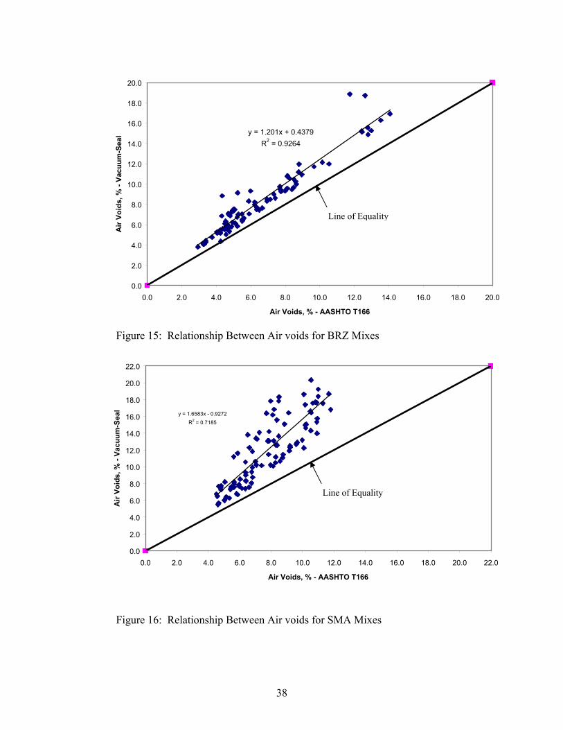
Figures 14 through 16 illustrate the relationships between air voids for TRZ, BRZ, and

SMA mixes, respectively. The results from the figures suggest that as density decreases

the bulk specific gravity measurements for the two methods become farther apart. The

33

results also indicate that as the gradation becomes coarser the data deviates farther from

the line of equality. This finding agrees with the research by Cooley et al. (12) when

comparing the two methods. The apparent reason for the difference in the two test

methods is loss of water during density measurement and the surface texture. The loss of

water when blotting will result in a higher measured density than the actual density. The

surface texture can result in the vacuum seal device measuring a lower density than the

actual density. Since the vacuum seal device gives a good estimation of density at lower

air voids (this indicates that the surface texture does not affect the results), it is also

expected to provide good estimation at higher air voids (since the plastic sealer does not

penetrate the voids within the mixture. Therefore, for this study, the density determined

from the vacuum seal device was used in the analysis (More discussion on density

measurement is provided in Volume II of this report).

34

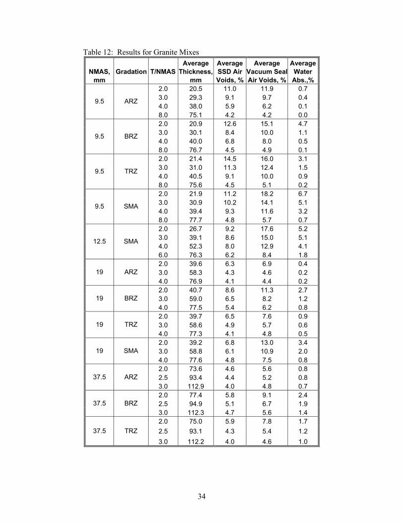
Table 12: Results for Granite Mixes Average Average Average Average NMAS, Gradation T/NMAS Thickness, SSD Air Vacuum Seal Water

mm mm Voids, % Air Voids, % Abs.,% 2.0 20.5 11.0 11.9 0.7 3.0 29.3 9.1 9.7 0.4 4.0 38.0 5.9 6.2 0.1

9.5 ARZ

8.0 75.1 4.2 4.2 0.0 2.0 20.9 12.6 15.1 4.7 3.0 30.1 8.4 10.0 1.1 4.0 40.0 6.8 8.0 0.5

9.5 BRZ

8.0 76.7 4.5 4.9 0.1 2.0 21.4 14.5 16.0 3.1 3.0 31.0 11.3 12.4 1.5 4.0 40.5 9.1 10.0 0.9

9.5 TRZ

8.0 75.6 4.5 5.1 0.2 2.0 21.9 11.2 18.2 6.7 3.0 30.9 10.2 14.1 5.1 4.0 39.4 9.3 11.6 3.2

9.5 SMA

8.0 77.7 4.8 5.7 0.7 2.0 26.7 9.2 17.6 5.2 3.0 39.1 8.6 15.0 5.1 4.0 52.3 8.0 12.9 4.1

12.5 SMA

6.0 76.3 6.2 8.4 1.8 2.0 39.6 6.3 6.9 0.4 3.0 58.3 4.3 4.6 0.2 19 ARZ 4.0 76.9 4.1 4.4 0.2 2.0 40.7 8.6 11.3 2.7 3.0 59.0 6.5 8.2 1.2 19 BRZ 4.0 77.5 5.4 6.2 0.8 2.0 39.7 6.5 7.6 0.9 3.0 58.6 4.9 5.7 0.6 19 TRZ 4.0 77.3 4.1 4.8 0.5 2.0 39.2 6.8 13.0 3.4 3.0 58.8 6.1 10.9 2.0 19 SMA 4.0 77.6 4.8 7.5 0.8 2.0 73.6 4.6 5.6 0.8 2.5 93.4 4.4 5.2 0.8 37.5 ARZ 3.0 112.9 4.0 4.8 0.7 2.0 77.4 5.8 9.1 2.4 2.5 94.9 5.1 6.7 1.9 37.5 BRZ 3.0 112.3 4.7 5.6 1.4 2.0 75.0 5.9 7.8 1.7 2.5 93.1 4.3 5.4 1.2 37.5 TRZ 3.0 112.2 4.0 4.6 1.0

35

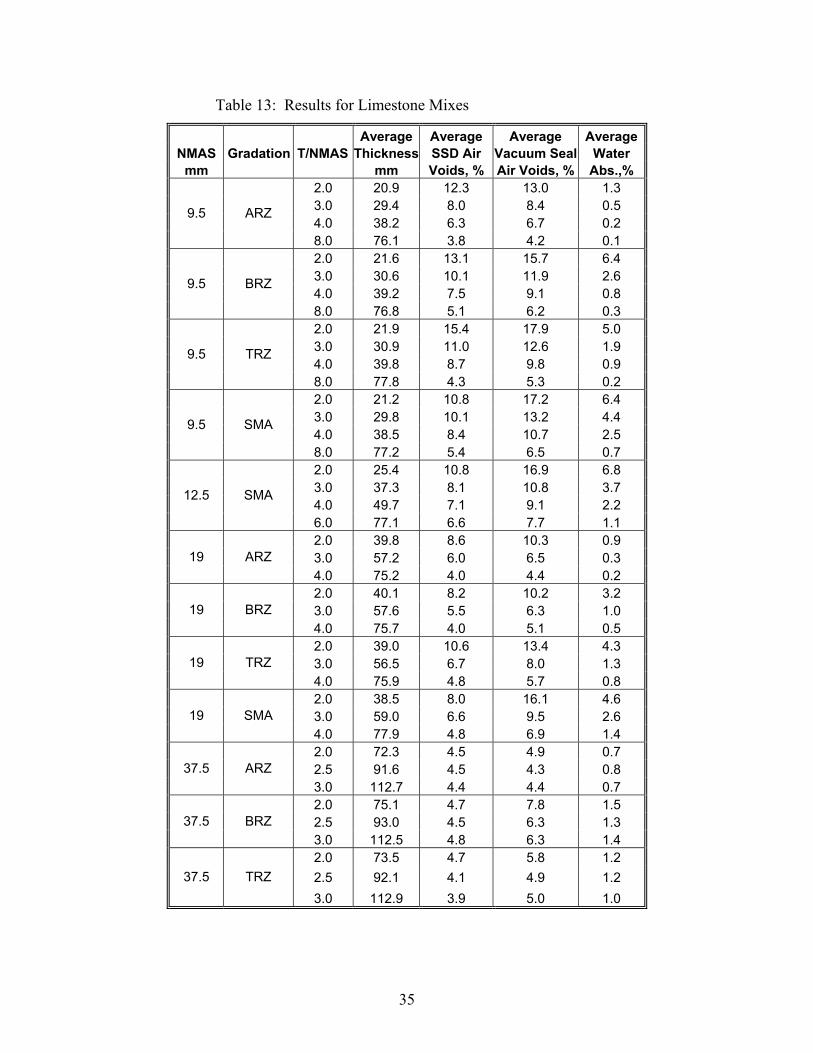
Table 13: Results for Limestone Mixes

Average Average Average Average NMAS Gradation T/NMAS Thickness SSD Air Vacuum Seal Water


9.5 ARZ

8.0 76.1 3.8 4.2 0.1 2.0 21.6 13.1 15.7 6.4 3.0 30.6 10.1 11.9 2.6 4.0 39.2 7.5 9.1 0.8

9.5 BRZ

8.0 76.8 5.1 6.2 0.3 2.0 21.9 15.4 17.9 5.0 3.0 30.9 11.0 12.6 1.9 4.0 39.8 8.7 9.8 0.9

9.5 TRZ

8.0 77.8 4.3 5.3 0.2 2.0 21.2 10.8 17.2 6.4 3.0 29.8 10.1 13.2 4.4 4.0 38.5 8.4 10.7 2.5

9.5 SMA

8.0 77.2 5.4 6.5 0.7 2.0 25.4 10.8 16.9 6.8 3.0 37.3 8.1 10.8 3.7 4.0 49.7 7.1 9.1 2.2

12.5 SMA


36

Table 14: Results for Gravel Mixes

Average Average Average Average NMAS Gradation T/NMAS Thickness, SSD Air Vacuum Seal Water


9.5 ARZ

8.0 73.9 4.0 4.0 0.1 2.0 21.3 12.8 18.2 4.1 3.0 29.7 8.5 9.8 1.3 4.0 38.7 6.6 7.7 0.6

9.5 BRZ

8.0 74.1 3.3 4.3 0.2 2.0 20.8 12.0 13.4 1.7 3.0 29.9 8.2 8.7 0.6 4.0 38.9 6.3 7.0 0.2

9.5 TRZ

8.0 76.4 4.1 4.4 0.1 2.0 21.1 10.7 19.4 6.0 3.0 30.3 10.4 15.0 5.1 4.0 38.3 9.3 12.4 3.5

9.5 SMA

8.0 77.4 5.8 6.8 0.9 2.0 27.2 8.2 17.6 5.0 3.0 38.5 8.0 13.6 4.0 4.0 52.7 7.7 11.5 3.7

12.5 SMA


37

y = 1.0576x + 0.0992R2 = 0.9887

0.0

2.0

4.0

6.0

8.0

10.0

12.0

14.0

16.0

0.0 2.0 4.0 6.0 8.0 10.0 12.0 14.0 16.0

Air Voids, % - AASHTO T166

Air

Void

s, %

- Va

cuum

-Sea

l

Figure 13: Relationship Between Air voids for ARZ Mixes

y = 1.1074x + 0.3893R2 = 0.978

0.0

2.0

4.0

6.0

8.0

10.0

12.0

14.0

16.0

18.0

20.0

0.0 2.0 4.0 6.0 8.0 10.0 12.0 14.0 16.0 18.0 20.0


Air

Void

s, %

- Va

cuum

-Sea

l

Figure 14: Relationship Between Air voids for TRZ Mixes

Line of Equality

Line of Equality

38

y = 1.201x + 0.4379R2 = 0.9264

0.0

2.0

4.0

6.0

8.0

10.0

12.0

14.0

16.0

18.0

20.0

0.0 2.0 4.0 6.0 8.0 10.0 12.0 14.0 16.0 18.0 20.0


Air

Void

s, %

- Va

cuum

-Sea

l

Figure 15: Relationship Between Air voids for BRZ Mixes

y = 1.6583x - 0.9272R2 = 0.7185

0.0

2.0

4.0

6.0

8.0

10.0

12.0

14.0

16.0

18.0

20.0

22.0

0.0 2.0 4.0 6.0 8.0 10.0 12.0 14.0 16.0 18.0 20.0 22.0


Air

Void

s, %

- Va

cuum

-Sea

l

Figure 16: Relationship Between Air voids for SMA Mixes

Line of Equality

Line of Equality

39

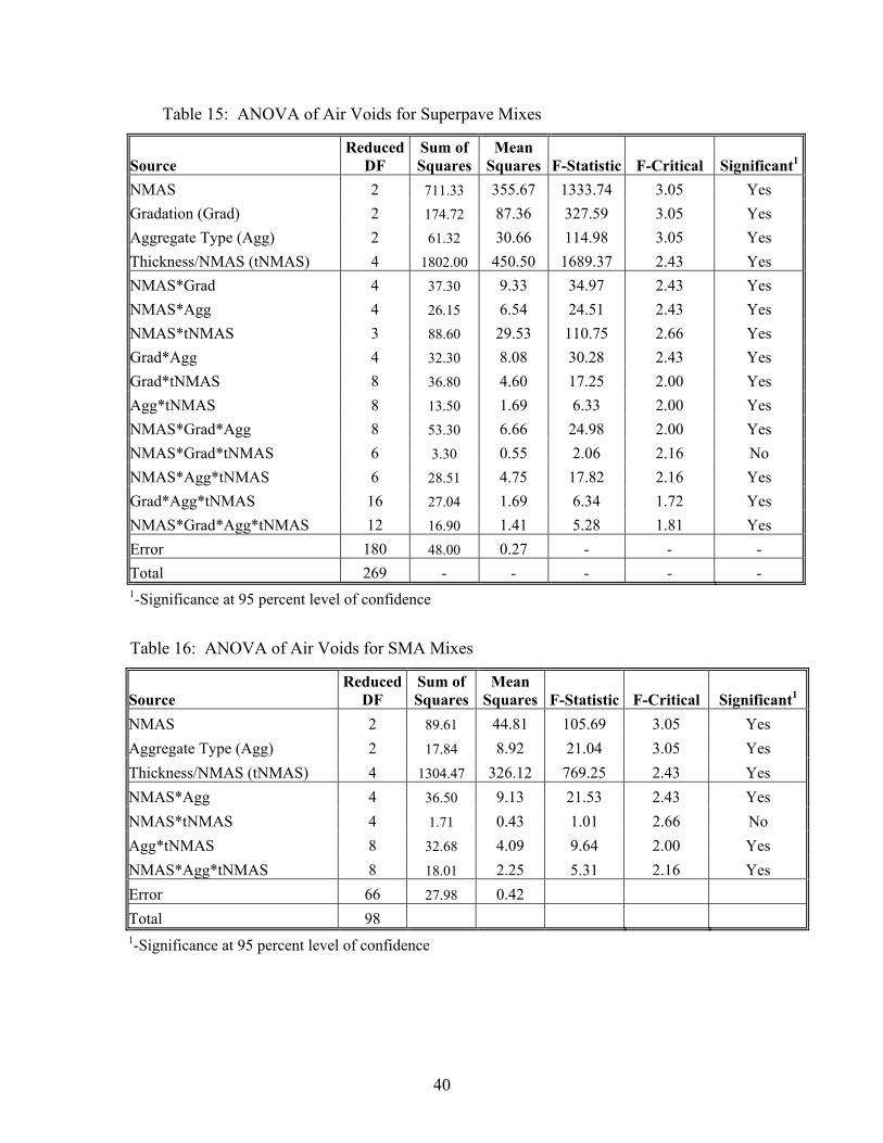
An analysis of variance (ANOVA) was performed to determine which factors

(aggregate type, NMAS, gradation shape, and t/NMAS) significantly affect the resulting

air void contents. Since Superpave and SMA mixes are very different, an ANOVA was

conducted for each mix type; the results are presented in Tables 15 and 16. Since this

study was designed in an unbalanced manner where the t/NMASs used were not the same

for each NMAS mix, the reduced degree of freedom (reduced DF) was used in the

analysis. The results show all factors and all interactions have a significant effect on the

air void contents except three-way interactions of NMAS*Grad*t/NMAS. T/NMAS has

the greatest impact followed by NMAS, gradation, and aggregate type.

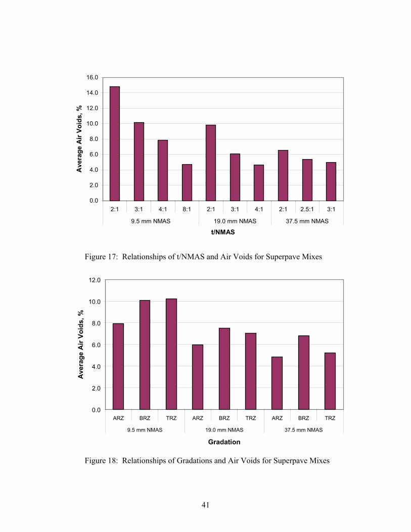
Figure 17 shows the impact of t/NMAS on the air voids. The plot indicates that as

the t/NMAS increases the air voids decrease for a given NMAS. The impact of gradation

on air voids for Superpave mixes is illustrated in Figure 18. The relationship is

interesting in that the ARZ mixes had the lowest air voids compared to the TRZ and BRZ

mixes for a given NMAS. This result could also suggest that fine-graded mixes are easier

to compact compared to coarse-graded.

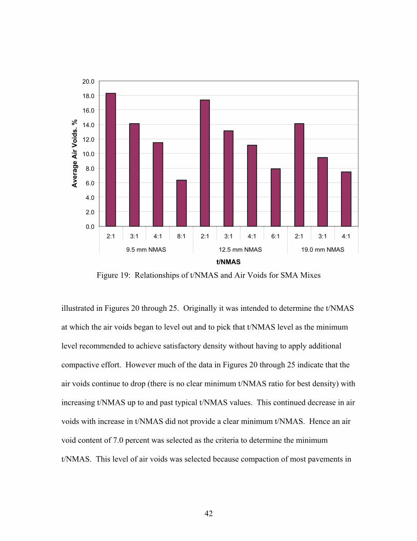
For the SMA mixes, the ANOVA results indicate that all factors and all interactions

except the two-way interaction of t/NMAS*NMAS have a significant impact on the air

voids. T/NMAS has the largest impact on the air voids followed by NMAS and

aggregate type. Figure 19 illustrates the relationship between t/NMAS and air voids. The

plot suggests that as t/NMAS increased the air voids decreased.

The main objective of this part of the study was to determine the minimum t/NMAS.

To achieve this objective, relationships of average air voids for the three aggregate types

versus t/NMAS with respect to NMAS and gradation were evaluated; the results are

40

Table 15: ANOVA of Air Voids for Superpave Mixes

Source Reduced

DF Sum of Squares

Mean Squares F-Statistic F-Critical Significant1

NMAS 2 711.33 355.67 1333.74 3.05 Yes Gradation (Grad) 2 174.72 87.36 327.59 3.05 Yes Aggregate Type (Agg) 2 61.32 30.66 114.98 3.05 Yes Thickness/NMAS (tNMAS) 4 1802.00 450.50 1689.37 2.43 Yes NMAS*Grad 4 37.30 9.33 34.97 2.43 Yes NMAS*Agg 4 26.15 6.54 24.51 2.43 Yes NMAS*tNMAS 3 88.60 29.53 110.75 2.66 Yes Grad*Agg 4 32.30 8.08 30.28 2.43 Yes Grad*tNMAS 8 36.80 4.60 17.25 2.00 Yes Agg*tNMAS 8 13.50 1.69 6.33 2.00 Yes NMAS*Grad*Agg 8 53.30 6.66 24.98 2.00 Yes NMAS*Grad*tNMAS 6 3.30 0.55 2.06 2.16 No NMAS*Agg*tNMAS 6 28.51 4.75 17.82 2.16 Yes Grad*Agg*tNMAS 16 27.04 1.69 6.34 1.72 Yes NMAS*Grad*Agg*tNMAS 12 16.90 1.41 5.28 1.81 Yes Error 180 48.00 0.27 - - - Total 269 - - - - - 1-Significance at 95 percent level of confidence

Table 16: ANOVA of Air Voids for SMA Mixes

Source Reduced

DF Sum of Squares

Mean Squares F-Statistic F-Critical Significant1

NMAS 2 89.61 44.81 105.69 3.05 Yes Aggregate Type (Agg) 2 17.84 8.92 21.04 3.05 Yes Thickness/NMAS (tNMAS) 4 1304.47 326.12 769.25 2.43 Yes NMAS*Agg 4 36.50 9.13 21.53 2.43 Yes NMAS*tNMAS 4 1.71 0.43 1.01 2.66 No Agg*tNMAS 8 32.68 4.09 9.64 2.00 Yes NMAS*Agg*tNMAS 8 18.01 2.25 5.31 2.16 Yes Error 66 27.98 0.42 Total 98 1-Significance at 95 percent level of confidence

41

0.0

2.0

4.0

6.0

8.0

10.0

12.0

14.0

16.0

2:1 3:1 4:1 8:1 2:1 3:1 4:1 2:1 2.5:1 3:1

9.5 mm NMAS 19.0 mm NMAS 37.5 mm NMAS

t/NMAS

Ave

rage

Air

Void

s, %

Figure 17: Relationships of t/NMAS and Air Voids for Superpave Mixes

0.0

2.0

4.0

6.0

8.0

10.0

12.0

ARZ BRZ TRZ ARZ BRZ TRZ ARZ BRZ TRZ


Gradation

Ave

rage

Air

Void

s, %

Figure 18: Relationships of Gradations and Air Voids for Superpave Mixes

42

0.0

2.0

4.0

6.0

8.0

10.0

12.0

14.0

16.0

18.0

20.0

2:1 3:1 4:1 8:1 2:1 3:1 4:1 6:1 2:1 3:1 4:1


t/NMAS

Ave

rage

Air

Void

s. %

Figure 19: Relationships of t/NMAS and Air Voids for SMA Mixes

illustrated in Figures 20 through 25. Originally it was intended to determine the t/NMAS

at which the air voids began to level out and to pick that t/NMAS level as the minimum

level recommended to achieve satisfactory density without having to apply additional

compactive effort. However much of the data in Figures 20 through 25 indicate that the

air voids continue to drop (there is no clear minimum t/NMAS ratio for best density) with

increasing t/NMAS up to and past typical t/NMAS values. This continued decrease in air

voids with increase in t/NMAS did not provide a clear minimum t/NMAS. Hence an air

void content of 7.0 percent was selected as the criteria to determine the minimum

t/NMAS. This level of air voids was selected because compaction of most pavements in

43

the field is targeted at 92.0 to 94.0 percent of theoretical maximum density. This

approach did not provide a sufficient comfort level for selecting a minimum t/NMAS,

hence, it was decided to compact some samples with a laboratory vibratory compactor

and when this data was not very conclusive it was further decided to compact some mixes

in the field at various t/NMAS ratios during reconstruction of the NCAT test track. It

was not originally planned to conduct tests with the laboratory vibratory compactor or

with the field mixes but during the study it was determined that an adequate answer could

not be determined from the Superpave gyratory compactor test plan so this additional

work was performed to provide a better overall answer. These two efforts are discussed

later in the report.

A characteristic of the Superpave gyratory compactor is that it applies a constant

strain to the mix, and the force required to produce this strain varies as necessary

depending on the stiffness of the mixture. This is not the approach that is observed in the

field where the stress is constant and the strain varies. Hence, the Superpave gyratory

compactor might not provide a reasonable answer since it differs from field compaction.

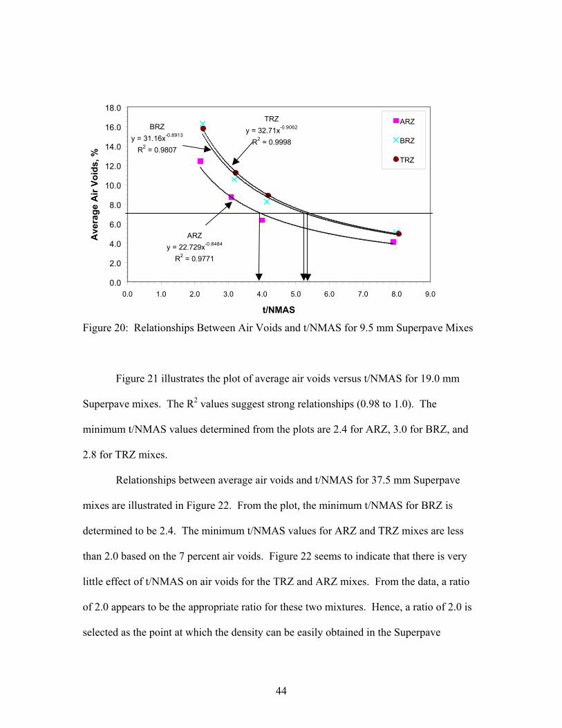
Figure 20 illustrates the plot of air voids versus t/NMAS for 9.5 mm Superpave

mixes. The best fit lines indicate that as the t/NMAS increases the air voids decrease. A

review of the data indicated that a power function provided the best fit. The coefficients

of determination (R2) values indicate strong relationships (0.98 to 1.0). The minimum

t/NMAS values to provide 7.0 percent air voids are 3.9 for ARZ, 5.2 for BRZ, and 5.4 for

TRZ mixes.

44

ARZy = 22.729x-0.8484

R2 = 0.9771

BRZy = 31.16x-0.8913

R2 = 0.9807

TRZy = 32.71x-0.9062

R2 = 0.9998

0.0

2.0

4.0

6.0

8.0

10.0

12.0

14.0

16.0

18.0

0.0 1.0 2.0 3.0 4.0 5.0 6.0 7.0 8.0 9.0

t/NMAS

Ave

rage

Air

Void

s, %

ARZ

BRZ

TRZ

Figure 20: Relationships Between Air Voids and t/NMAS for 9.5 mm Superpave Mixes

Figure 21 illustrates the plot of average air voids versus t/NMAS for 19.0 mm

Superpave mixes. The R2 values suggest strong relationships (0.98 to 1.0). The

minimum t/NMAS values determined from the plots are 2.4 for ARZ, 3.0 for BRZ, and

2.8 for TRZ mixes.

Relationships between average air voids and t/NMAS for 37.5 mm Superpave

mixes are illustrated in Figure 22. From the plot, the minimum t/NMAS for BRZ is

determined to be 2.4. The minimum t/NMAS values for ARZ and TRZ mixes are less

than 2.0 based on the 7 percent air voids. Figure 22 seems to indicate that there is very

little effect of t/NMAS on air voids for the TRZ and ARZ mixes. From the data, a ratio

of 2.0 appears to be the appropriate ratio for these two mixtures. Hence, a ratio of 2.0 is

selected as the point at which the density can be easily obtained in the Superpave

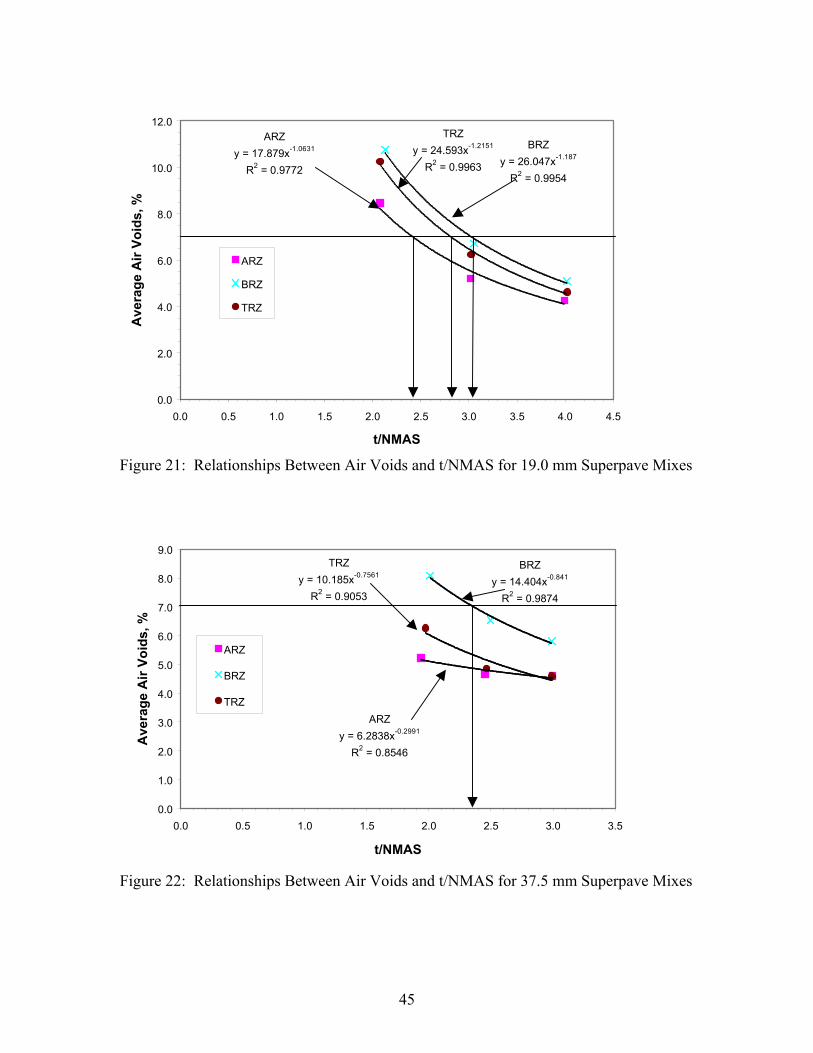
45

ARZy = 17.879x-1.0631

R2 = 0.9772

BRZy = 26.047x-1.187

R2 = 0.9954

TRZy = 24.593x-1.2151

R2 = 0.9963

0.0

2.0

4.0

6.0

8.0

10.0

12.0

0.0 0.5 1.0 1.5 2.0 2.5 3.0 3.5 4.0 4.5

t/NMAS

Ave

rage

Air

Void

s, %

ARZ

BRZ

TRZ


ARZy = 6.2838x-0.2991

R2 = 0.8546

BRZy = 14.404x-0.841

R2 = 0.9874

TRZy = 10.185x-0.7561

R2 = 0.9053

0.0

1.0

2.0

3.0

4.0

5.0

6.0

7.0

8.0

9.0

0.0 0.5 1.0 1.5 2.0 2.5 3.0 3.5

t/NMAS

Ave

rage

Air

Void

s, %

ARZ

BRZ

TRZ


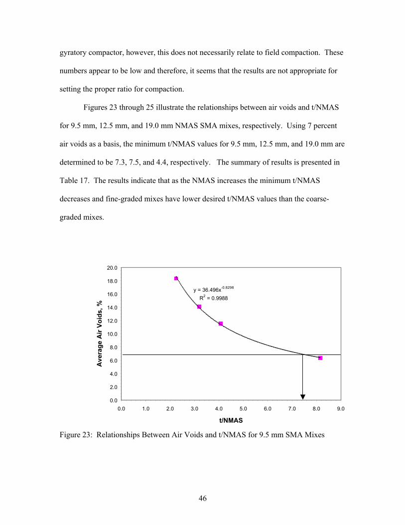
46

gyratory compactor, however, this does not necessarily relate to field compaction. These

numbers appear to be low and therefore, it seems that the results are not appropriate for

setting the proper ratio for compaction.

Figures 23 through 25 illustrate the relationships between air voids and t/NMAS

for 9.5 mm, 12.5 mm, and 19.0 mm NMAS SMA mixes, respectively. Using 7 percent

air voids as a basis, the minimum t/NMAS values for 9.5 mm, 12.5 mm, and 19.0 mm are

determined to be 7.3, 7.5, and 4.4, respectively. The summary of results is presented in

Table 17. The results indicate that as the NMAS increases the minimum t/NMAS

decreases and fine-graded mixes have lower desired t/NMAS values than the coarse-

graded mixes.

y = 36.496x-0.8298

R2 = 0.9988

0.0

2.0

4.0

6.0

8.0

10.0

12.0

14.0

16.0

18.0

20.0

0.0 1.0 2.0 3.0 4.0 5.0 6.0 7.0 8.0 9.0

t/NMAS

Ave

rage

Air

Void

s, %

Figure 23: Relationships Between Air Voids and t/NMAS for 9.5 mm SMA Mixes

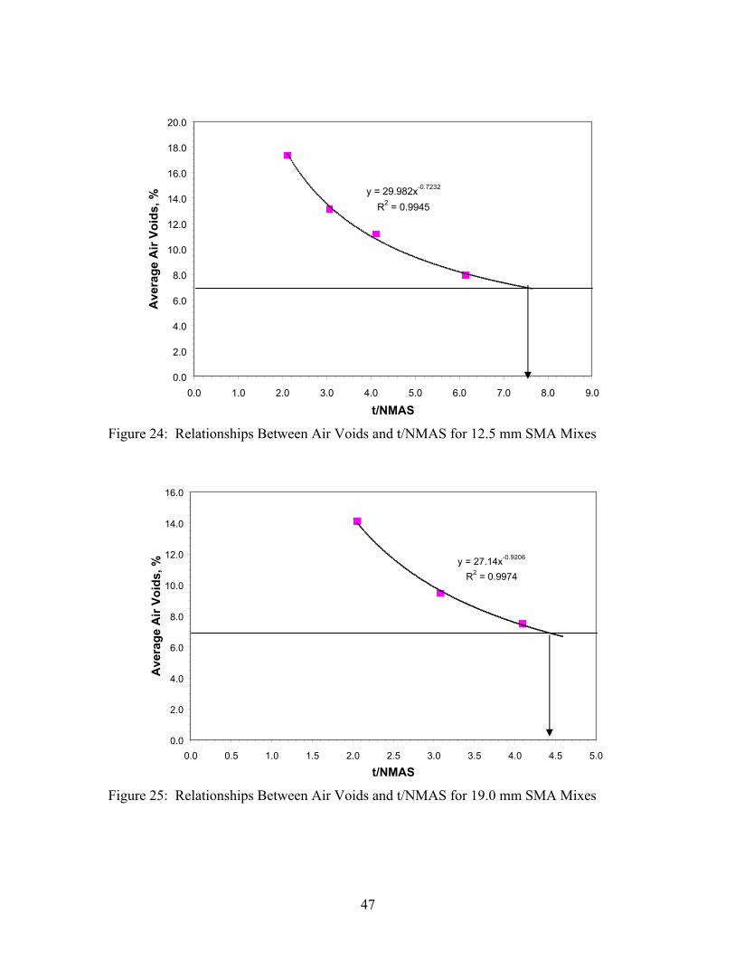
47

y = 29.982x-0.7232

R2 = 0.9945

0.0

2.0

4.0

6.0

8.0

10.0

12.0

14.0

16.0

18.0

20.0

0.0 1.0 2.0 3.0 4.0 5.0 6.0 7.0 8.0 9.0

t/NMAS

Ave

rage

Air

Void

s, %


y = 27.14x-0.9206

R2 = 0.9974

0.0

2.0

4.0

6.0

8.0

10.0

12.0

14.0

16.0

0.0 0.5 1.0 1.5 2.0 2.5 3.0 3.5 4.0 4.5 5.0

t/NMAS

Ave

rage

Air

Void

s, %


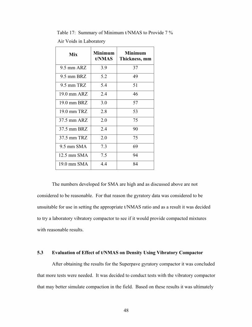
48

Table 17: Summary of Minimum t/NMAS to Provide 7 %

Air Voids in Laboratory

Mix Minimum t/NMAS

Minimum Thickness, mm

9.5 mm ARZ 3.9 37

9.5 mm BRZ 5.2 49

9.5 mm TRZ 5.4 51

19.0 mm ARZ 2.4 46

19.0 mm BRZ 3.0 57

19.0 mm TRZ 2.8 53

37.5 mm ARZ 2.0 75

37.5 mm BRZ 2.4 90

37.5 mm TRZ 2.0 75

9.5 mm SMA 7.3 69

12.5 mm SMA 7.5 94

19.0 mm SMA 4.4 84

The numbers developed for SMA are high and as discussed above are not

considered to be reasonable. For that reason the gyratory data was considered to be

unsuitable for use in setting the appropriate t/NMAS ratio and as a result it was decided

to try a laboratory vibratory compactor to see if it would provide compacted mixtures

with reasonable results.

5.3 Evaluation of Effect of t/NMAS on Density Using Vibratory Compactor

After obtaining the results for the Superpave gyratory compactor it was concluded

that more tests were needed. It was decided to conduct tests with the vibratory compactor

that may better simulate compaction in the field. Based on these results it was ultimately

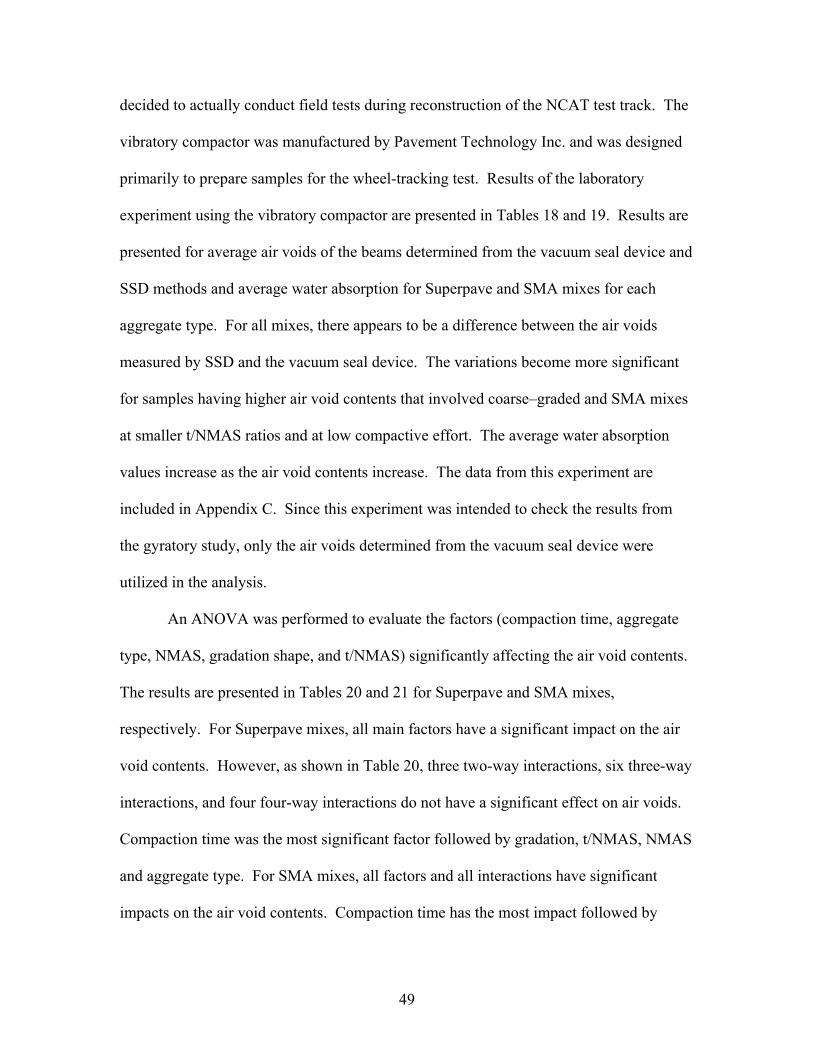
49

decided to actually conduct field tests during reconstruction of the NCAT test track. The

vibratory compactor was manufactured by Pavement Technology Inc. and was designed

primarily to prepare samples for the wheel-tracking test. Results of the laboratory

experiment using the vibratory compactor are presented in Tables 18 and 19. Results are

presented for average air voids of the beams determined from the vacuum seal device and

SSD methods and average water absorption for Superpave and SMA mixes for each

aggregate type. For all mixes, there appears to be a difference between the air voids

measured by SSD and the vacuum seal device. The variations become more significant

for samples having higher air void contents that involved coarse–graded and SMA mixes

at smaller t/NMAS ratios and at low compactive effort. The average water absorption

values increase as the air void contents increase. The data from this experiment are

included in Appendix C. Since this experiment was intended to check the results from

the gyratory study, only the air voids determined from the vacuum seal device were

utilized in the analysis.

An ANOVA was performed to evaluate the factors (compaction time, aggregate

type, NMAS, gradation shape, and t/NMAS) significantly affecting the air void contents.

The results are presented in Tables 20 and 21 for Superpave and SMA mixes,

respectively. For Superpave mixes, all main factors have a significant impact on the air

void contents. However, as shown in Table 20, three two-way interactions, six three-way

interactions, and four four-way interactions do not have a significant effect on air voids.

Compaction time was the most significant factor followed by gradation, t/NMAS, NMAS

and aggregate type. For SMA mixes, all factors and all interactions have significant

impacts on the air void contents. Compaction time has the most impact followed by

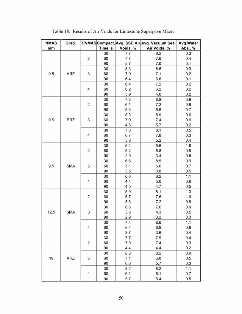
50

Table 18: Results of Air Voids for Limestone Superpave Mixes

NMAS Grad. T/NMAS Compact. Avg. SSD Air Avg. Vacuum Seal Avg.Water mm Time, s Voids, % Air Voids, % Abs., %

30 7.7 8.2 0.3 2 60 7.7 7.6 0.4 90 5.7 7.0 0.1 30 8.3 8.6 0.3

9.5 ARZ 3 60 7.0 7.1 0.2 90 6.4 6.6 0.1 30 6.4 7.2 0.2 4 60 6.2 6.2 0.2 90 3.9 4.0 0.2 30 7.3 8.8 0.9 2 60 6.1 7.2 0.9 90 5.3 6.6 0.7 30 8.3 8.9 0.6

9.5 BRZ 3 60 7.0 7.4 0.9 90 4.8 5.7 0.2 30 7.8 8.1 0.5 4 60 6.7 7.8 0.3 90 5.0 5.2 0.4 30 6.4 9.6 1.6 2 60 5.2 5.8 0.9 90 2.9 3.4 0.6 30 6.6 8.5 0.9

9.5 SMA 3 60 5.1 6.0 0.7 90 3.5 3.8 0.5 30 6.6 8.2 1.1 4 60 4.4 5.0 0.6 90 4.5 4.7 0.5 30 5.9 8.1 1.3 2 60 5.7 7.6 1.0 90 5.8 7.2 0.8 30 6.8 7.6 0.9

12.5 SMA 3 60 3.6 4.3 0.5 90 2.9 3.2 0.3 30 7.4 8.6 1.1 4 60 6.4 6.9 0.8 90 3.7 3.6 0.4 30 7.7 7.9 0.4 2 60 7.0 7.4 0.3 90 4.4 4.4 0.2 30 8.3 8.2 0.9

19 ARZ 3 60 7.1 6.8 0.5 90 6.0 5.7 0.3 30 8.2 8.2 1.1 4 60 6.1 6.1 0.7 90 5.7 5.4 0.5

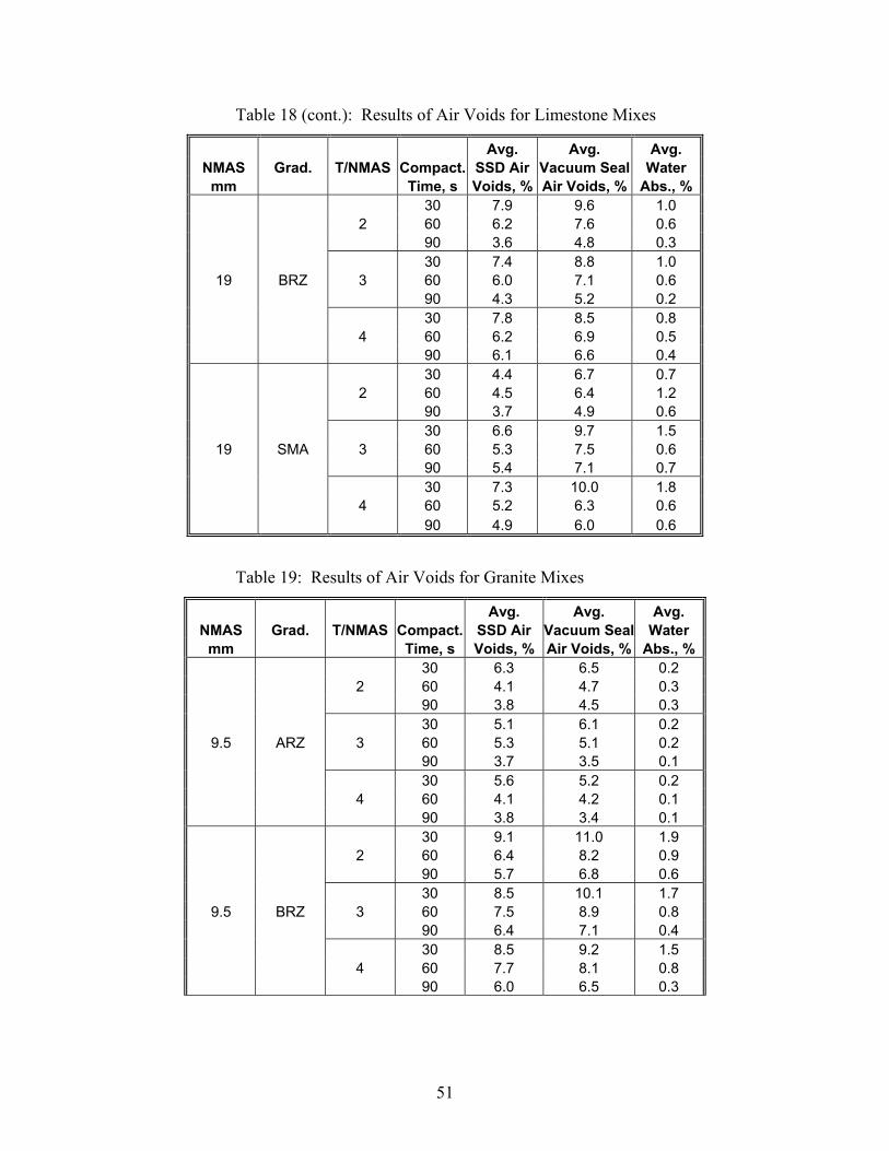
51

Table 18 (cont.): Results of Air Voids for Limestone Mixes

Avg. Avg. Avg. NMAS Grad. T/NMAS Compact. SSD Air Vacuum Seal Water

mm Time, s Voids, % Air Voids, % Abs., % 30 7.9 9.6 1.0 2 60 6.2 7.6 0.6 90 3.6 4.8 0.3 30 7.4 8.8 1.0

19 BRZ 3 60 6.0 7.1 0.6 90 4.3 5.2 0.2 30 7.8 8.5 0.8 4 60 6.2 6.9 0.5 90 6.1 6.6 0.4 30 4.4 6.7 0.7 2 60 4.5 6.4 1.2 90 3.7 4.9 0.6 30 6.6 9.7 1.5

19 SMA 3 60 5.3 7.5 0.6 90 5.4 7.1 0.7 30 7.3 10.0 1.8 4 60 5.2 6.3 0.6 90 4.9 6.0 0.6

Table 19: Results of Air Voids for Granite Mixes

Avg. Avg. Avg. NMAS Grad. T/NMAS Compact. SSD Air Vacuum Seal Water

mm Time, s Voids, % Air Voids, % Abs., % 30 6.3 6.5 0.2 2 60 4.1 4.7 0.3 90 3.8 4.5 0.3 30 5.1 6.1 0.2

9.5 ARZ 3 60 5.3 5.1 0.2 90 3.7 3.5 0.1 30 5.6 5.2 0.2 4 60 4.1 4.2 0.1 90 3.8 3.4 0.1 30 9.1 11.0 1.9 2 60 6.4 8.2 0.9 90 5.7 6.8 0.6 30 8.5 10.1 1.7

9.5 BRZ 3 60 7.5 8.9 0.8 90 6.4 7.1 0.4 30 8.5 9.2 1.5 4 60 7.7 8.1 0.8 90 6.0 6.5 0.3

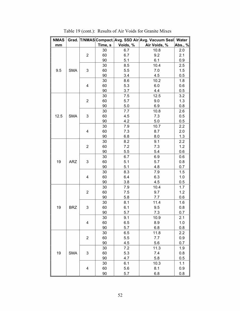
52

Table 19 (cont.): Results of Air Voids for Granite Mixes

NMAS Grad. T/NMAS Compact. Avg. SSD Air Avg. Vacuum Seal Water mm Time, s Voids, % Air Voids, % Abs., %

30 6.7 10.8 2.0 2 60 6.7 9.2 2.1 90 5.1 6.1 0.9 30 8.5 10.4 2.5

9.5 SMA 3 60 5.5 7.0 1.5 90 3.4 4.5 0.5 30 8.6 10.2 1.8 4 60 5.3 6.0 0.6 90 3.7 4.4 0.5 30 7.5 12.5 3.2 2 60 5.7 9.0 1.3 90 5.0 6.9 0.8 30 7.7 10.8 2.6

12.5 SMA 3 60 4.5 7.3 0.5 90 4.2 5.0 0.5 30 7.9 10.7 2.2 4 60 7.3 8.7 2.0 90 6.8 8.0 1.3 30 8.2 9.1 2.2 2 60 7.2 7.3 1.2 90 5.5 5.4 0.6 30 6.7 6.9 0.6

19 ARZ 3 60 5.1 5.7 0.8 90 5.1 4.8 0.7 30 8.3 7.9 1.5 4 60 6.4 6.3 1.0 90 3.8 4.5 0.5 30 7.9 10.4 1.7 2 60 7.5 9.7 1.2 90 5.8 7.7 0.6 30 8.1 11.4 1.6

19 BRZ 3 60 6.1 9.5 0.8 90 5.7 7.3 0.7 30 9.1 10.9 2.1 4 60 6.5 8.9 1.0 90 5.7 6.8 0.8 30 6.5 11.8 2.2 2 60 5.5 7.7 0.9 90 4.5 5.6 0.7 30 7.2 11.3 1.9

19 SMA 3 60 5.3 7.4 0.8 90 4.7 5.8 0.5 30 6.1 10.3 1.1 4 60 5.6 8.1 0.9 90 5.7 6.8 0.8

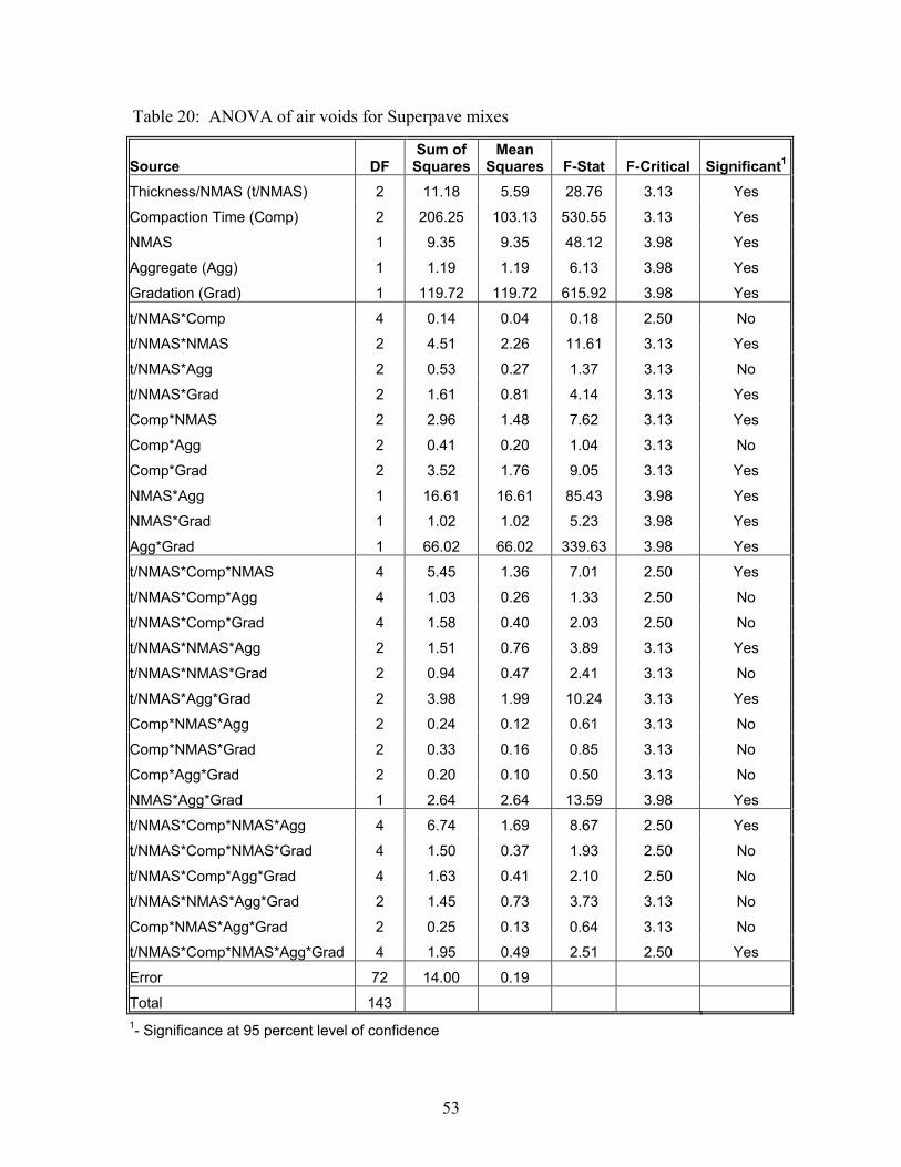
53

Table 20: ANOVA of air voids for Superpave mixes

Source DF Sum of

SquaresMean

Squares F-Stat F-Critical Significant1

Thickness/NMAS (t/NMAS) 2 11.18 5.59 28.76 3.13 Yes

Compaction Time (Comp) 2 206.25 103.13 530.55 3.13 Yes

NMAS 1 9.35 9.35 48.12 3.98 Yes

Aggregate (Agg) 1 1.19 1.19 6.13 3.98 Yes

Gradation (Grad) 1 119.72 119.72 615.92 3.98 Yes

t/NMAS*Comp 4 0.14 0.04 0.18 2.50 No

t/NMAS*NMAS 2 4.51 2.26 11.61 3.13 Yes

t/NMAS*Agg 2 0.53 0.27 1.37 3.13 No

t/NMAS*Grad 2 1.61 0.81 4.14 3.13 Yes

Comp*NMAS 2 2.96 1.48 7.62 3.13 Yes

Comp*Agg 2 0.41 0.20 1.04 3.13 No

Comp*Grad 2 3.52 1.76 9.05 3.13 Yes

NMAS*Agg 1 16.61 16.61 85.43 3.98 Yes

NMAS*Grad 1 1.02 1.02 5.23 3.98 Yes

Agg*Grad 1 66.02 66.02 339.63 3.98 Yes

t/NMAS*Comp*NMAS 4 5.45 1.36 7.01 2.50 Yes

t/NMAS*Comp*Agg 4 1.03 0.26 1.33 2.50 No

t/NMAS*Comp*Grad 4 1.58 0.40 2.03 2.50 No

t/NMAS*NMAS*Agg 2 1.51 0.76 3.89 3.13 Yes

t/NMAS*NMAS*Grad 2 0.94 0.47 2.41 3.13 No

t/NMAS*Agg*Grad 2 3.98 1.99 10.24 3.13 Yes

Comp*NMAS*Agg 2 0.24 0.12 0.61 3.13 No

Comp*NMAS*Grad 2 0.33 0.16 0.85 3.13 No

Comp*Agg*Grad 2 0.20 0.10 0.50 3.13 No

NMAS*Agg*Grad 1 2.64 2.64 13.59 3.98 Yes

t/NMAS*Comp*NMAS*Agg 4 6.74 1.69 8.67 2.50 Yes

t/NMAS*Comp*NMAS*Grad 4 1.50 0.37 1.93 2.50 No

t/NMAS*Comp*Agg*Grad 4 1.63 0.41 2.10 2.50 No

t/NMAS*NMAS*Agg*Grad 2 1.45 0.73 3.73 3.13 No

Comp*NMAS*Agg*Grad 2 0.25 0.13 0.64 3.13 No

t/NMAS*Comp*NMAS*Agg*Grad 4 1.95 0.49 2.51 2.50 Yes

Error 72 14.00 0.19

Total 143 1- Significance at 95 percent level of confidence

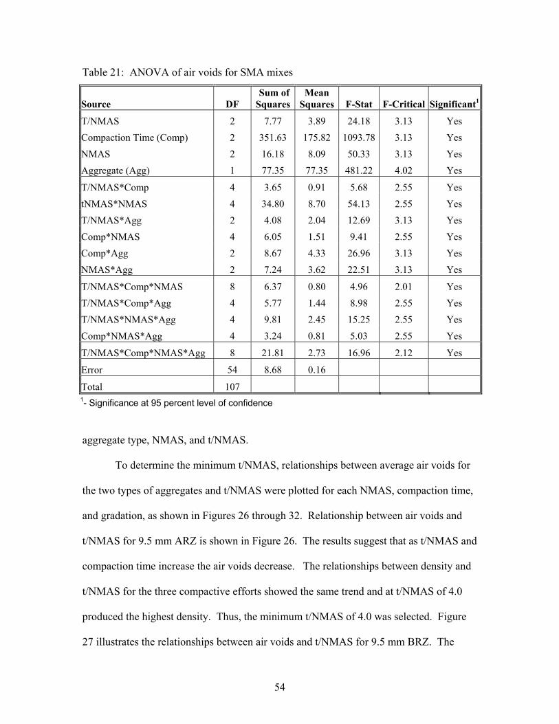
54

Table 21: ANOVA of air voids for SMA mixes

Source DF Sum of Squares

Mean Squares F-Stat F-Critical Significant1

T/NMAS 2 7.77 3.89 24.18 3.13 Yes Compaction Time (Comp) 2 351.63 175.82 1093.78 3.13 Yes NMAS 2 16.18 8.09 50.33 3.13 Yes Aggregate (Agg) 1 77.35 77.35 481.22 4.02 Yes

T/NMAS*Comp 4 3.65 0.91 5.68 2.55 Yes tNMAS*NMAS 4 34.80 8.70 54.13 2.55 Yes T/NMAS*Agg 2 4.08 2.04 12.69 3.13 Yes Comp*NMAS 4 6.05 1.51 9.41 2.55 Yes Comp*Agg 2 8.67 4.33 26.96 3.13 Yes NMAS*Agg 2 7.24 3.62 22.51 3.13 Yes

T/NMAS*Comp*NMAS 8 6.37 0.80 4.96 2.01 Yes T/NMAS*Comp*Agg 4 5.77 1.44 8.98 2.55 Yes T/NMAS*NMAS*Agg 4 9.81 2.45 15.25 2.55 Yes Comp*NMAS*Agg 4 3.24 0.81 5.03 2.55 Yes

T/NMAS*Comp*NMAS*Agg 8 21.81 2.73 16.96 2.12 Yes

Error 54 8.68 0.16

Total 107 1- Significance at 95 percent level of confidence

aggregate type, NMAS, and t/NMAS.

To determine the minimum t/NMAS, relationships between average air voids for

the two types of aggregates and t/NMAS were plotted for each NMAS, compaction time,

and gradation, as shown in Figures 26 through 32. Relationship between air voids and

t/NMAS for 9.5 mm ARZ is shown in Figure 26. The results suggest that as t/NMAS and

compaction time increase the air voids decrease. The relationships between density and

t/NMAS for the three compactive efforts showed the same trend and at t/NMAS of 4.0

produced the highest density. Thus, the minimum t/NMAS of 4.0 was selected. Figure

27 illustrates the relationships between air voids and t/NMAS for 9.5 mm BRZ. The

55

results indicate that thickness did not have a great effect on compaction. For compaction

time of 90 sec, the air voids at t/NMAS 2.0, 3.0, and 4.0 are approximately 6.0 percent

whereas for compaction time 60 and 30 sec, the air voids are approximately 8.0 percent

and 9.0 percent, respectively. Therefore, t/NMAS of 2.0 was selected as the minimum

t/NMAS. Figures 26 and 27 suggest that the BRZ mix was more difficult to compact

than ARZ mix for a given compactive effort. Figure 28 presents the relationship between

air voids and t/NMAS for 19.0 mm ARZ. The results suggest that t/NMAS basically did

not affect the compaction. A minimum t/NMAS of 2.0 was selected. Figure 29

illustrates the relationships between air voids and t/NMAS for 19.0 mm BRZ. The

figure indicates that thickness did not affect compaction. Thus, a minimum t/NMAS of

2.0 was suggested. Again, the BRZ mix was more difficult to compact than ARZ, as

shown in Figures 28 and 29.

The relationships between air voids and t/NMAS for 9.5 SMA is shown in Figure

30. The results indicate that t/NMAS affects the compaction at 60 sec compaction time

and not at 30 and 90 sec. This is likely due to random variation in the test results. From

the curve, the minimum t/NMAS was selected to be 3.0 Figure 31 shows the

relationships between air voids and t/NMAS for 12.5 mm SMA. The trend of the curve is

similar for the three compaction times. As the t/NMAS increased from 2.0 to 3.0 the air

voids decreased and started to increase as the t/NMAS increased from 3.0 to 4.0. A

minimum t/NMAS of 3.0 was suggested. Figures 30 and 31 also indicate that both 9.5

mm and 12.5 mm SMA mixes had about the same compactibility. The relationships

between air voids and t/NMAS for 19.0 mm SMA is presented in Figure 32. The trend of

the curves indicate that as t/NMAS increased from 2.0 to 3.0 the air voids increased and

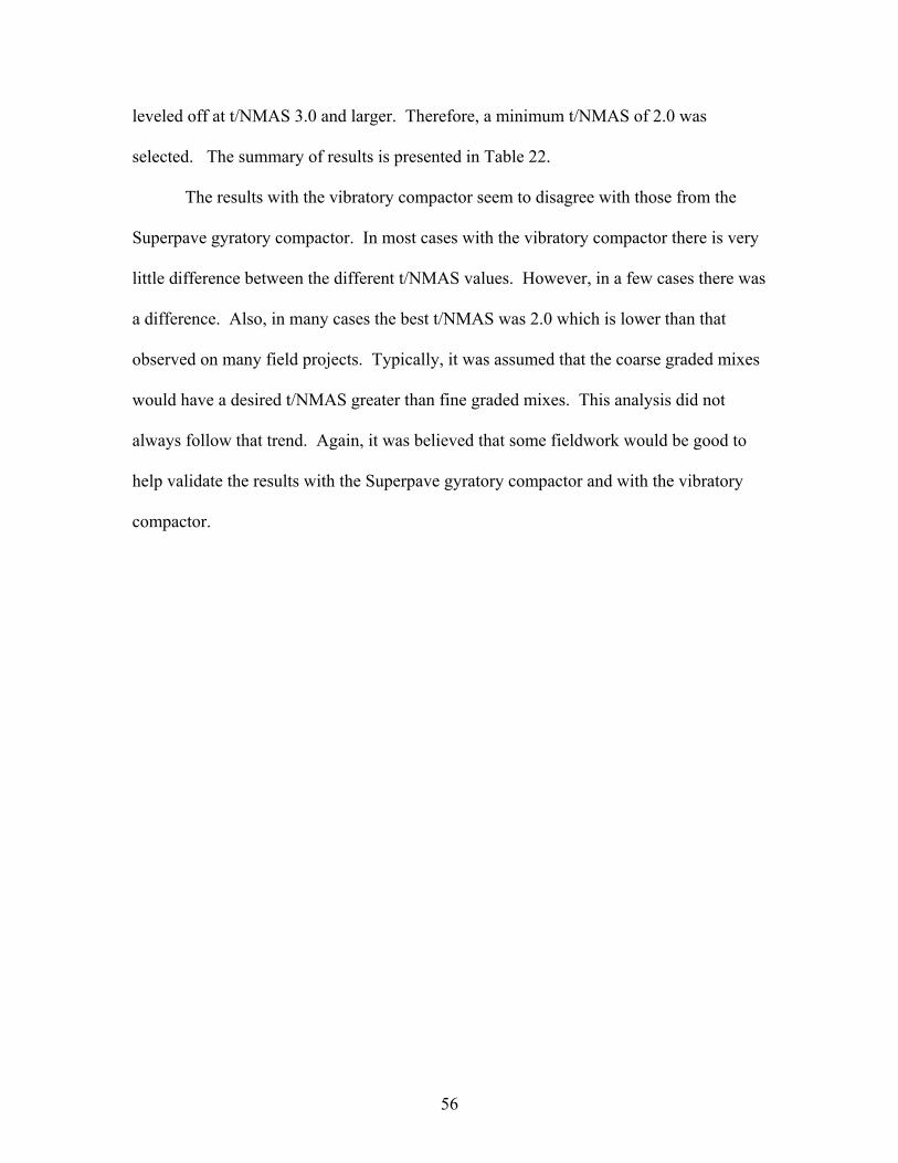
56

leveled off at t/NMAS 3.0 and larger. Therefore, a minimum t/NMAS of 2.0 was

selected. The summary of results is presented in Table 22.

The results with the vibratory compactor seem to disagree with those from the

Superpave gyratory compactor. In most cases with the vibratory compactor there is very

little difference between the different t/NMAS values. However, in a few cases there was

a difference. Also, in many cases the best t/NMAS was 2.0 which is lower than that

observed on many field projects. Typically, it was assumed that the coarse graded mixes

would have a desired t/NMAS greater than fine graded mixes. This analysis did not

always follow that trend. Again, it was believed that some fieldwork would be good to

help validate the results with the Superpave gyratory compactor and with the vibratory

compactor.

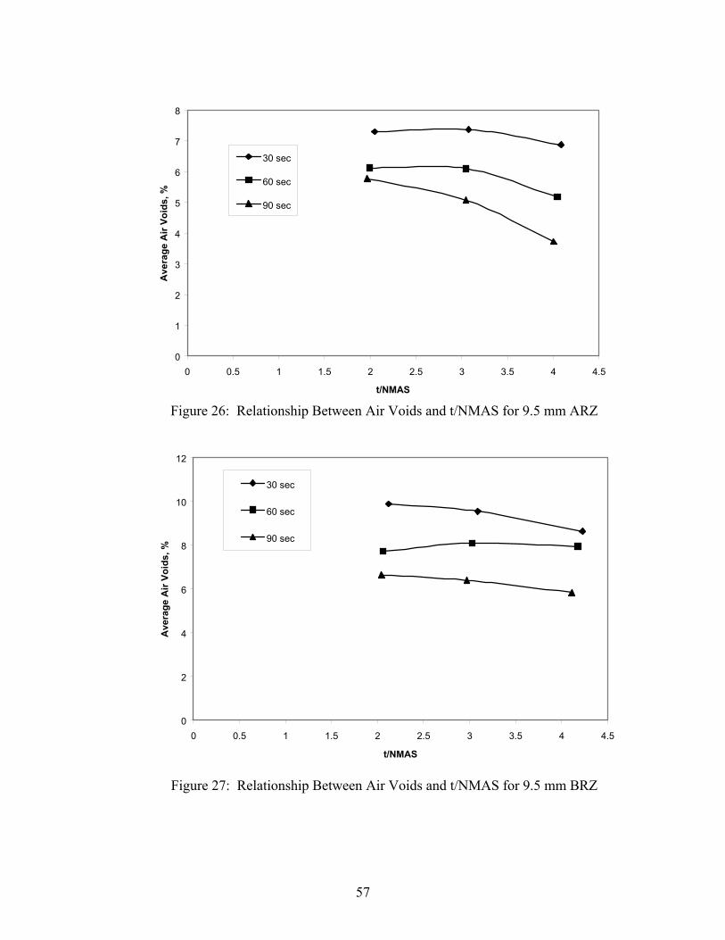
57

0

1

2

3

4

5

6

7

8

0 0.5 1 1.5 2 2.5 3 3.5 4 4.5

t/NMAS

Ave

rage

Air

Void

s, %

30 sec

60 sec

90 sec

Figure 26: Relationship Between Air Voids and t/NMAS for 9.5 mm ARZ

0

2

4

6

8

10

12

0 0.5 1 1.5 2 2.5 3 3.5 4 4.5

t/NMAS

Ave

rage

Air

Void

s, %

30 sec

60 sec

90 sec

Figure 27: Relationship Between Air Voids and t/NMAS for 9.5 mm BRZ

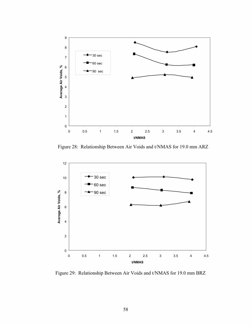
58

0

1

2

3

4

5

6

7

8

9

0 0.5 1 1.5 2 2.5 3 3.5 4 4.5

t/NMAS

Ave

rage

Air

Void

s, %

30 sec

60 sec

90 sec

Figure 28: Relationship Between Air Voids and t/NMAS for 19.0 mm ARZ

0

2

4

6

8

10

12

0 0.5 1 1.5 2 2.5 3 3.5 4 4.5

t/NMAS

Ave

rage

Air

Void

s, %

30 sec

60 sec

90 sec

Figure 29: Relationship Between Air Voids and t/NMAS for 19.0 mm BRZ

59

0

2

4

6

8

10

12

0 0.5 1 1.5 2 2.5 3 3.5 4 4.5

t/NMAS

Ave

rae

Air

Void

s, %

30s 60s 90s

Figure 30: Relationship Between Air Voids and t/NMAS for 9.5 mm SMA

0.0

2.0

4.0

6.0

8.0

10.0

12.0

0 0.5 1 1.5 2 2.5 3 3.5 4 4.5

t/NMAS

Ave

rage

Air

Void

s, %

30s 60s 90s


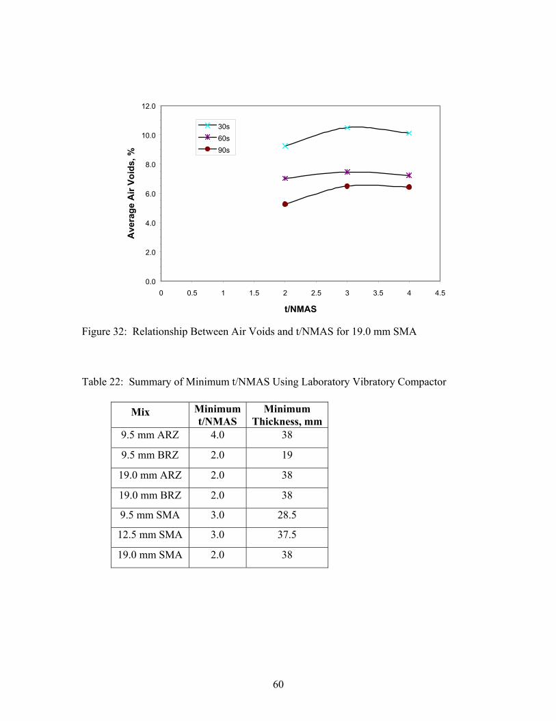
60

0.0

2.0

4.0

6.0

8.0

10.0

12.0

0 0.5 1 1.5 2 2.5 3 3.5 4 4.5

t/NMAS

Ave

rage

Air

Void

s, %

30s 60s 90s


Table 22: Summary of Minimum t/NMAS Using Laboratory Vibratory Compactor

Mix Minimum t/NMAS

Minimum Thickness, mm

9.5 mm ARZ 4.0 38

9.5 mm BRZ 2.0 19

19.0 mm ARZ 2.0 38

19.0 mm BRZ 2.0 38

9.5 mm SMA 3.0 28.5

12.5 mm SMA 3.0 37.5

19.0 mm SMA 2.0 38

61

5.4 Evaluation of Effect of t/NMAS on Density from Field Study

The field test sections consisted of seven mixes that were to be placed during the

2003 reconstruction of the NCAT test track. These mixes had to be field verified before

they were placed. Hence, some of the mixes did not meet volumetrics and other

requirements but they were judged to be sufficient for this part of the study since

determining the desired thickness range was a relative value based on t/NMAS.

5.4.1 Section 1

Section 1 was constructed on July 18, 2003 and consisted of a t/NMAS that

ranged from 2.0 to 5.0 and placed over an existing HMA layer. This construction was

performed adjacent to the NCAT Test Track. The mix consisted of a 9.5 mm NMAS

fine-graded mixture. The length of the section was about 40 m and the width was about

3.5 m. On some of the sections the placement began on the thick side and in some cases

the rolling began on the thin side. This technique was used so that there would be no bias

due to the placement of the HMA. On this section the paving began with the thicker

portion of the section and the thickness was slowly decreased as the paver moved down

the test lane. The desired mat thickness was achieved by gradually adjusting the screed

depth crank of the paver during the paving operation. The weather conditions during the

paving were 84oF, overcast, with calm wind. The existing surface temperature was also

84oF.

The roller utilized in this section was an 11 ton steel roller HYPAC C778B with

78 in. drum width that could operate in vibratory or static mode. The rubber tire roller

available did not meet desired requirements for weight and tire pressure and thus the data

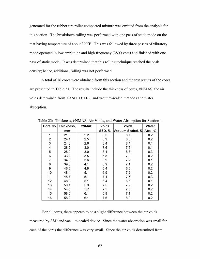
62

generated for the rubber tire roller compacted mixture was omitted from the analysis for

this section. The breakdown rolling was performed with one pass of static mode on the

mat having temperature of about 300oF. This was followed by three passes of vibratory

mode operated in low amplitude and high frequency (3800 vpm) and finished with one

pass of static mode. It was determined that this rolling technique reached the peak

density; hence, additional rolling was not performed.

A total of 16 cores were obtained from this section and the test results of the cores

are presented in Table 23. The results include the thickness of cores, t/NMAS, the air

voids determined from AASHTO T166 and vacuum-sealed methods and water

absorption.

Table 23: Thickness, t/NMAS, Air Voids, and Water Absorption for Section 1

Core No. Thickness, t/NMAS Voids Voids Water mm SSD, % Vacuum Sealed, % Abs., % 1 21.0 2.2 8.5 8.7 0.2 2 24.1 2.5 8.9 8.8 0.2 3 24.3 2.6 8.4 8.4 0.1 4 28.2 3.0 7.6 7.6 0.1 5 28.9 3.0 8.1 8.3 0.3 6 33.2 3.5 6.8 7.0 0.2 7 34.3 3.6 6.9 7.2 0.1 8 39.0 4.1 6.9 7.1 0.2 9 46.6 4.9 6.4 6.6 0.2

10 48.4 5.1 6.9 7.2 0.2 11 48.7 5.1 7.1 7.5 0.3 12 48.9 5.1 6.4 6.5 0.1 13 50.1 5.3 7.5 7.9 0.2 14 54.0 5.7 7.5 7.8 0.2 15 58.0 6.1 6.9 7.1 0.2 16 58.2 6.1 7.6 8.0 0.2

For all cores, there appears to be a slight difference between the air voids

measured by SSD and vacuum-sealed device. Since the water absorption was small for

each of the cores the difference was very small. Since the air voids determined from

63

vacuum-sealed device was used in the analysis for the previous part in this research, it

was decided to utilize the air voids from vacuum sealed device in this analysis for

consistency. This is assumed to be the most accurate measure of density. To determine

the minimum t/NMAS for this mix, the relationship of air voids and thickness was

evaluated and the result illustrated in Figure 33.

A review of the data indicated that a polynomial function provided the best fit.

The best-fit line indicates that as the thickness increased the air voids decreased until a

point where additional thickness resulted in an increase in air voids. The recommended

thickness range was selected as the point(s) where the air voids increased by 0.5 %. This

number is somewhat arbitrary but it is realistic. Therefore, as shown in Figure 33, the

recommended thickness range for 9.5 mm fine-graded mix is 32 to 55 mm. This does not

mean that compaction cannot be obtained when outside of these limits but it is an

indication that more compactive effort would be needed. So this recommended range

should only be used as a guide and should not be a rigid requirement. The effect of

t/NMAS on the measured density was determined from Figure 33. Data in the figure

indicates that the lowest air voids (7.0% air voids) occurred at t/NMAS of 4.4. At a ratio

of 2 the void level was 2.5% higher, at a ratio of 3 the void level was 1.0% higher, at a

ratio of 4 the void level was 0.1% higher and at a ratio of 5 the void level was 0.1%

higher.

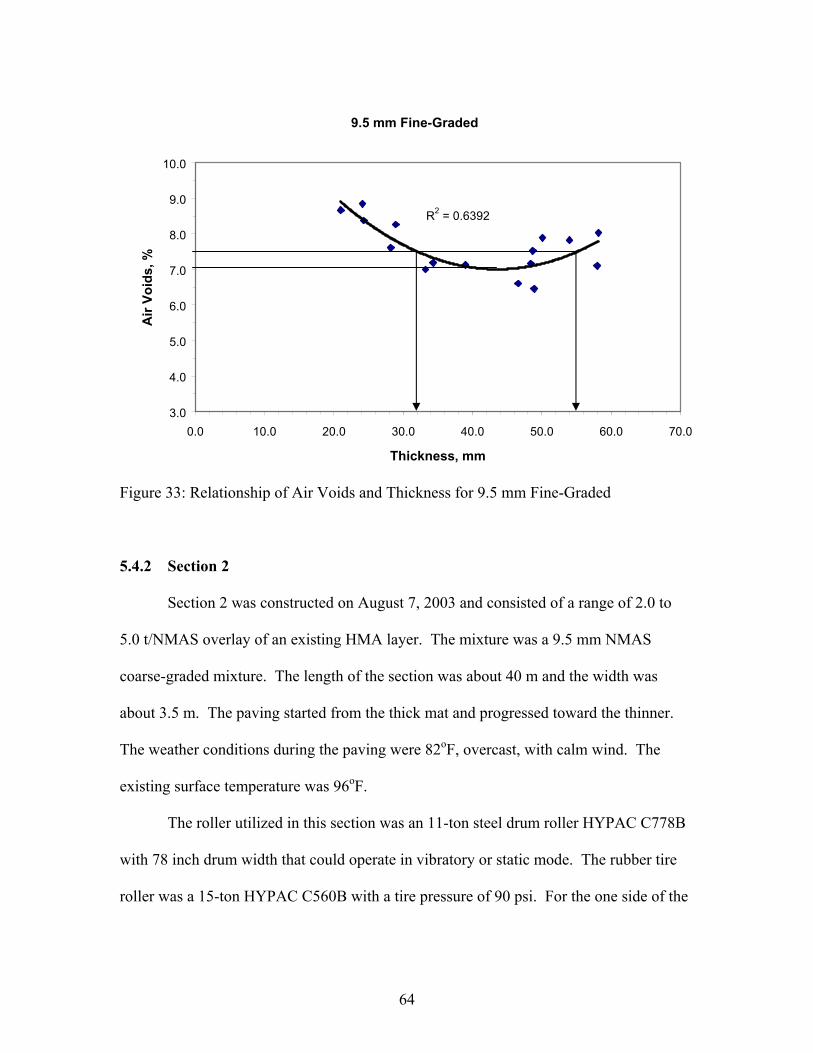
64

9.5 mm Fine-Graded

R2 = 0.6392

3.0

4.0

5.0

6.0

7.0

8.0

9.0

10.0

0.0 10.0 20.0 30.0 40.0 50.0 60.0 70.0

Thickness, mm

Air

Void

s, %

Figure 33: Relationship of Air Voids and Thickness for 9.5 mm Fine-Graded

5.4.2 Section 2

Section 2 was constructed on August 7, 2003 and consisted of a range of 2.0 to

5.0 t/NMAS overlay of an existing HMA layer. The mixture was a 9.5 mm NMAS

coarse-graded mixture. The length of the section was about 40 m and the width was

about 3.5 m. The paving started from the thick mat and progressed toward the thinner.

The weather conditions during the paving were 82oF, overcast, with calm wind. The

existing surface temperature was 96oF.

The roller utilized in this section was an 11-ton steel drum roller HYPAC C778B

with 78 inch drum width that could operate in vibratory or static mode. The rubber tire

roller was a 15-ton HYPAC C560B with a tire pressure of 90 psi. For the one side of the

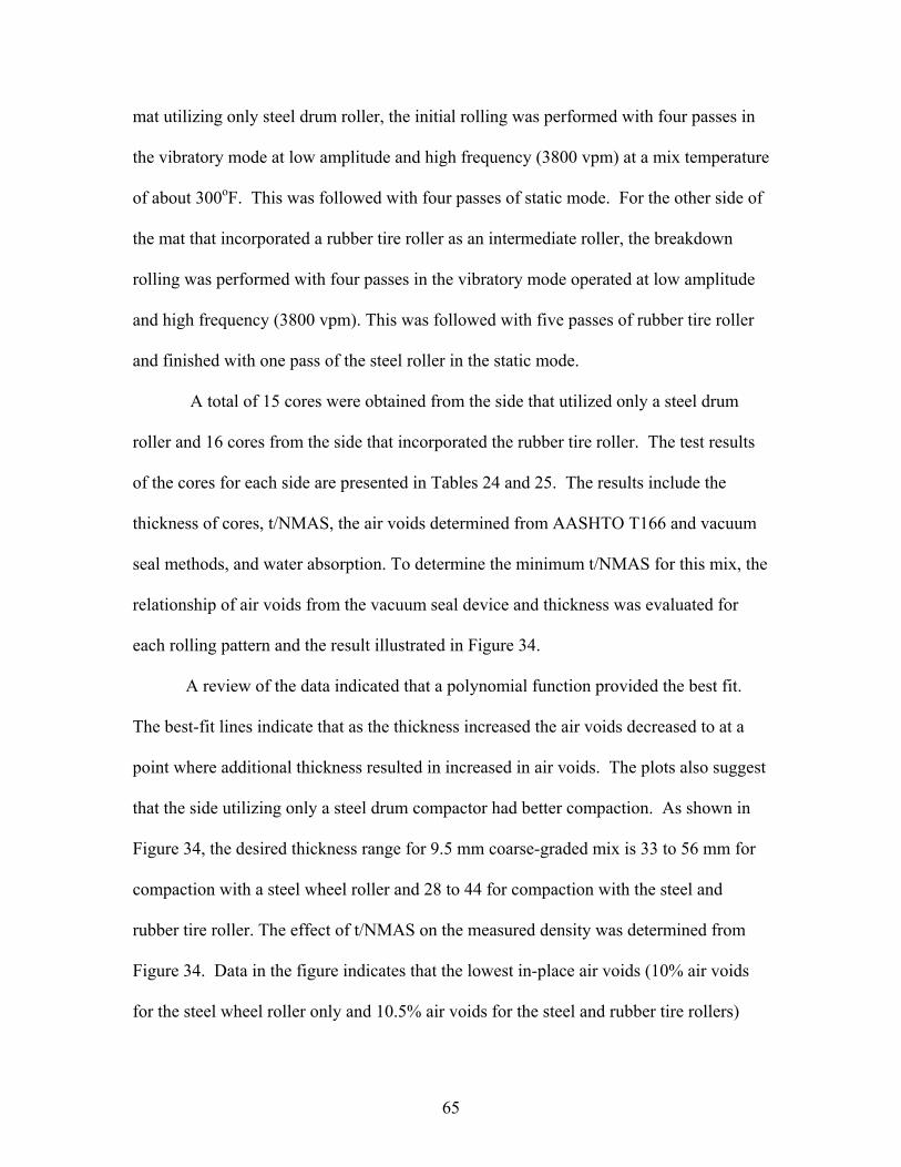
65

mat utilizing only steel drum roller, the initial rolling was performed with four passes in

the vibratory mode at low amplitude and high frequency (3800 vpm) at a mix temperature

of about 300oF. This was followed with four passes of static mode. For the other side of

the mat that incorporated a rubber tire roller as an intermediate roller, the breakdown

rolling was performed with four passes in the vibratory mode operated at low amplitude

and high frequency (3800 vpm). This was followed with five passes of rubber tire roller

and finished with one pass of the steel roller in the static mode.

A total of 15 cores were obtained from the side that utilized only a steel drum

roller and 16 cores from the side that incorporated the rubber tire roller. The test results

of the cores for each side are presented in Tables 24 and 25. The results include the

thickness of cores, t/NMAS, the air voids determined from AASHTO T166 and vacuum

seal methods, and water absorption. To determine the minimum t/NMAS for this mix, the

relationship of air voids from the vacuum seal device and thickness was evaluated for

each rolling pattern and the result illustrated in Figure 34.


The best-fit lines indicate that as the thickness increased the air voids decreased to at a

point where additional thickness resulted in increased in air voids. The plots also suggest

that the side utilizing only a steel drum compactor had better compaction. As shown in

Figure 34, the desired thickness range for 9.5 mm coarse-graded mix is 33 to 56 mm for

compaction with a steel wheel roller and 28 to 44 for compaction with the steel and

rubber tire roller. The effect of t/NMAS on the measured density was determined from

Figure 34. Data in the figure indicates that the lowest in-place air voids (10% air voids

for the steel wheel roller only and 10.5% air voids for the steel and rubber tire rollers)

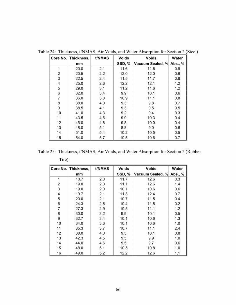
66

Table 24: Thickness, t/NMAS, Air Voids, and Water Absorption for Section 2 (Steel) Core No. Thickness, t/NMAS Voids Voids Water

mm SSD, % Vacuum Sealed, % Abs., % 1 20.0 2.1 11.6 11.6 0.9 2 20.5 2.2 12.0 12.0 0.6 3 22.5 2.4 11.5 11.7 0.9 4 25.0 2.6 12.2 12.1 1.2 5 29.0 3.1 11.2 11.6 1.2 6 32.0 3.4 9.9 10.1 0.6 7 36.0 3.8 10.9 11.1 0.8 8 38.0 4.0 9.3 9.8 0.7 9 38.5 4.1 9.3 9.5 0.5

10 41.0 4.3 9.2 9.4 0.3 11 43.5 4.6 9.9 10.3 0.4 12 46.0 4.8 9.8 10.0 0.4 13 48.0 5.1 8.8 9.0 0.6 14 51.0 5.4 10.2 10.5 0.5 15 54.0 5.7 10.5 10.6 0.7

Table 25: Thickness, t/NMAS, Air Voids, and Water Absorption for Section 2 (Rubber

Tire)


10 34.0 3.6 10.1 10.6 1.0 11 35.3 3.7 10.7 11.1 2.4 12 38.0 4.0 9.5 10.1 0.8 13 42.3 4.5 9.5 9.9 1.0 14 44.0 4.6 9.5 9.7 0.6 15 48.0 5.1 10.5 10.8 1.0 16 49.0 5.2 12.2 12.6 1.1

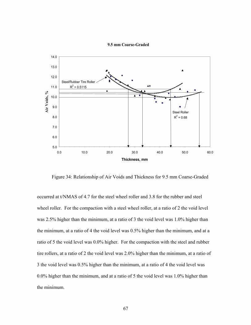
67

Figure 34: Relationship of Air Voids and Thickness for 9.5 mm Coarse-Graded

occurred at t/NMAS of 4.7 for the steel wheel roller and 3.8 for the rubber and steel

wheel roller. For the compaction with a steel wheel roller, at a ratio of 2 the void level

was 2.5% higher than the minimum, at a ratio of 3 the void level was 1.0% higher than

the minimum, at a ratio of 4 the void level was 0.5% higher than the minimum, and at a

ratio of 5 the void level was 0.0% higher. For the compaction with the steel and rubber

tire rollers, at a ratio of 2 the void level was 2.0% higher than the minimum, at a ratio of

3 the void level was 0.5% higher than the minimum, at a ratio of 4 the void level was

0.0% higher than the minimum, and at a ratio of 5 the void level was 1.0% higher than

the minimum.

9.5 mm Coarse-Graded

Steel RollerR2 = 0.68

Steel/Rubber Tire RollerR2 = 0.5115

5.0

6.0

7.0

8.0

9.0

10.0

11.0

12.0

13.0

14.0

0.0 10.0 20.0 30.0 40.0 50.0 60.0

Thickness, mm

Air

Voi

ds, %

68

5.4.3 Section 3

Section 3 was constructed on July 25, 2003 and ranged from a t/NMAS of 2.0 to

5.0 placed over an existing HMA layer. The mix was a 9.5 mm NMAS SMA. The

length of the section was about 40 m and the width was about 3.5 m. The paving started

from the thick mat and progressed to the thinner mat. The desired mat thickness was

achieved by gradually adjusting the screed depth crank of the paver during the operation.

The weather conditions during the paving were 95oF, partly cloudy, with calm wind. The

existing surface temperature was 115oF.


with 78 in. wide drum that could operate in vibratory or static mode. The rubber tire

roller was a 15-ton HYPAC C560B with a tire pressure of 90 psi. For the side of the mat

utilizing only the steel drum roller, the initial rolling was performed with one pass of

static rolling continued with five passes of vibratory mode operated in low amplitude and

high frequency (3800 vpm) on the mat having temperature of about 320oF. This was

followed with two passes of static mode for the finish rolling. For the other side of the

mat that incorporated a rubber tire roller as an intermediate roller, the breakdown rolling

was performed with one pass of static and three passes of vibratory mode operated in low

amplitude and high frequency (3800 vpm). This was followed with eight passes of rubber

tire roller and finished with two passes of steel roller in static mode.

A total of 12 cores were obtained from the side that utilized only the steel drum

roller and another 12 cores from the side that incorporated the rubber tire roller. The test

results of the cores for each side are presented in Tables 26 and 27. The results include

the thickness of cores, t/NMAS, the air voids determined from AASHTO T166 and

69

vacuum seal methods, and water absorption. To determine the range of recommended

t/NMAS for this mix, the relationship of air voids from Vacuum seal device and

thickness was evaluated for each rolling pattern and the results are illustrated in Figure

35.


The best-fit lines indicate that as the thickness increased the air voids decreased to a point

where additional thickness resulted in increased air voids. The plots also suggest that the

side utilizing only the steel drum compactor had better compaction. Rubber tire rollers

are not used on SMA mixtures and this data confirms that there is no need to use the

rubber tire roller. As shown in Figure 35, the recommended range for thickness for the

9.5 mm SMA mix is 36 to 50 mm for the compaction with a steel wheel roller and 25 to

48 mm for compaction with a steel and rubber tire roller. The effect of t/NMAS on the

measured density was determined from Figure 35. Data in the figure indicates that the

lowest in-place air voids (8.5% air voids for the steel wheel roller only and 10.3% air

voids for the steel and rubber tire rollers) occurred at t/NMAS of 4.5 for the steel wheel

roller and 3.8 for the rubber and steel wheel roller. For the compaction with a steel wheel

roller, at a ratio of 2 the void level was 5.5% higher than the minimum, at a ratio of 3 the

void level was 2.0% higher than the minimum, at a ratio of 4 the void level was 0.2%

higher than the minimum, and at a ratio of 5 the void level was 0.2% higher than the

minimum. For the compaction with the steel and rubber tire rollers, at a ratio of 2 the

void level was 1.2% higher than the minimum, at a ratio of 3 the void level was 0.2%

higher than the minimum, at a ratio of 4 the void level was 0.0% higher than the

minimum, and at a ratio of 5 the void level was 0.5% higher than the minimum.

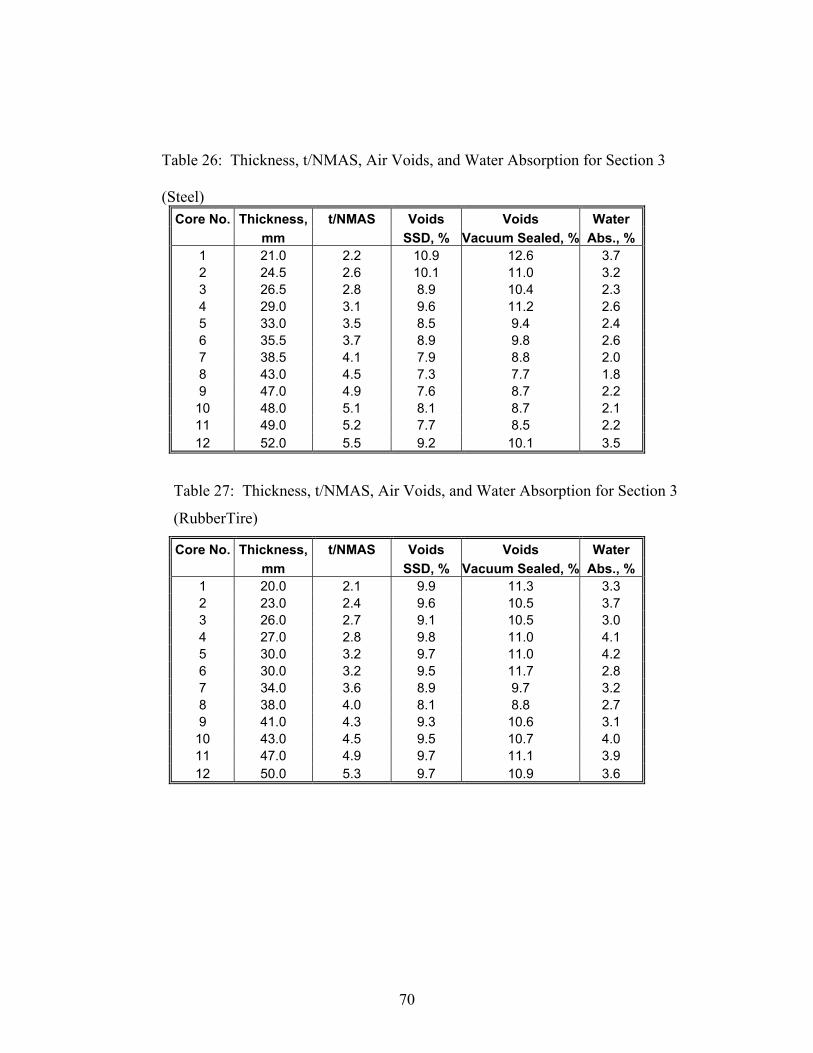
70


(Steel)


10 48.0 5.1 8.1 8.7 2.1 11 49.0 5.2 7.7 8.5 2.2 12 52.0 5.5 9.2 10.1 3.5


(RubberTire)


10 43.0 4.5 9.5 10.7 4.0 11 47.0 4.9 9.7 11.1 3.9 12 50.0 5.3 9.7 10.9 3.6

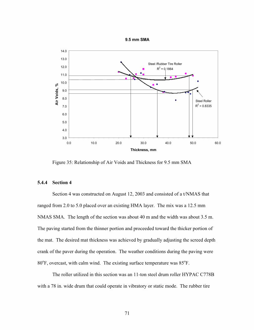
71

Figure 35: Relationship of Air Voids and Thickness for 9.5 mm SMA

5.4.4 Section 4

Section 4 was constructed on August 12, 2003 and consisted of a t/NMAS that

ranged from 2.0 to 5.0 placed over an existing HMA layer. The mix was a 12.5 mm

NMAS SMA. The length of the section was about 40 m and the width was about 3.5 m.

The paving started from the thinner portion and proceeded toward the thicker portion of

the mat. The desired mat thickness was achieved by gradually adjusting the screed depth

crank of the paver during the operation. The weather conditions during the paving were

80oF, overcast, with calm wind. The existing surface temperature was 85oF.


with a 78 in. wide drum that could operate in vibratory or static mode. The rubber tire

9.5 mm SMA


Steel /Rubber Tire RollerR2 = 0.1864

3.0

4.0

5.0

6.0

7.0

8.0

9.0

10.0

11.0

12.0

13.0

14.0

0.0 10.0 20.0 30.0 40.0 50.0 60.0

Thickness, mm

Air

Void

s, %

72



the vibratory mode operated at low amplitude and high frequency (3800 vpm). The mat

temperature was approximately 320oF. This was followed with three passes in the static

mode including finish rolling. For the other side of the mat that incorporated a rubber tire

roller as an intermediate roller, the initial rolling was performed with four passes in the

vibratory mode operated at low amplitude and high frequency (3800 vpm). This was

followed with four passes of the rubber tire roller and finished with one pass of steel

roller in the static mode.




thickness of cores, n/NMAS, the air voids determined from AASHTO T166 and vacuum-

sealed methods, and water absorption. To determine the recommended t/NMAS for this

mix, the relationship of air voids from the vacuum sealed device and thickness was

evaluated for each rolling pattern and the results were illustrated in Figure 36.

The best-fit lines indicate that as the thickness increased the air voids decreased

until a point where excessive thickness resulted in increased air voids. The plots also

suggest that the side utilizing only the steel drum compactor had better compaction. As

shown in Figure 36, the suggested minimum thickness for 12.5 mm SMA mix is 48 for

compaction with steel wheel roller and 57 for compaction with steel and rubber tire

rollers. For these mixes the densification was still increasing as the t/NMAS was

increasing even at the thicker portions. Also the curve did not fit the data as well as

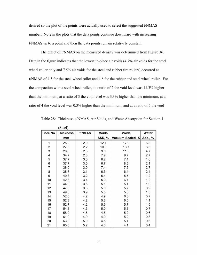
73

desired so the plot of the points were actually used to select the suggested t/NMAS

number. Note in the plots that the data points continue downward with increasing

t/NMAS up to a point and then the data points remain relatively constant.

The effect of t/NMAS on the measured density was determined from Figure 36.

Data in the figure indicates that the lowest in-place air voids (4.7% air voids for the steel

wheel roller only and 7.5% air voids for the steel and rubber tire rollers) occurred at

t/NMAS of 4.5 for the steel wheel roller and 4.8 for the rubber and steel wheel roller. For

the compaction with a steel wheel roller, at a ratio of 2 the void level was 11.3% higher

than the minimum, at a ratio of 3 the void level was 3.3% higher than the minimum, at a

ratio of 4 the void level was 0.3% higher than the minimum, and at a ratio of 5 the void


(Steel)


10 42.3 3.4 5.0 6.7 1.2 11 44.0 3.5 5.1 5.1 1.0 12 47.0 3.8 5.0 5.7 0.9 13 49.0 3.9 5.5 5.6 1.3 14 52.0 4.2 4.9 6.6 0.7 15 52.3 4.2 5.3 6.0 1.1 16 52.7 4.2 5.6 5.7 1.5 17 54.3 4.3 5.0 5.6 0.7 18 58.0 4.6 4.5 5.2 0.6 19 61.0 4.9 4.9 5.2 0.8 20 63.0 5.0 4.5 5.1 0.6 21 65.0 5.2 4.0 4.1 0.4

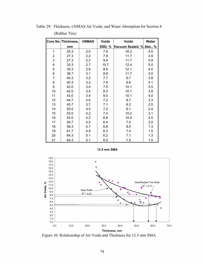
74

Table 29: Thickness, t/NMAS Air Voids, and Water Absorption for Section 4

(Rubber Tire)

Core No. Thickness, t/NMAS Voids Voids Water mm SSD, % Vacuum Sealed, % Abs., % 1 25.3 2.0 7.6 16.2 4.0 2 27.3 2.2 7.9 11.7 3.9 3 27.3 2.2 9.4 11.7 5.9 4 33.3 2.7 10.7 12.4 5.0 5 35.3 2.8 8.6 12.1 4.0 6 38.7 3.1 8.8 11.7 5.0 7 40.3 3.2 7.7 9.7 3.8 8 40.3 3.2 7.8 9.6 4.1 9 42.0 3.4 7.5 10.1 3.5 10 42.0 3.4 8.3 10.1 3.9 11 43.0 3.4 8.0 10.1 4.0 12 44.7 3.6 7.2 8.7 3.3 13 45.7 3.7 7.1 8.2 2.0 14 50.0 4.0 7.2 8.1 2.4 15 53.0 4.2 7.4 10.2 3.1 16 53.0 4.2 6.8 10.0 2.0 17 55.7 4.5 6.4 7.0 2.0 18 59.3 4.7 6.8 8.0 1.3 19 61.7 4.9 6.3 7.4 1.5 20 64.3 5.1 6.2 7.1 1.3 21 64.3 5.1 6.5 7.5 1.5

Figure 36: Relationship of Air Voids and Thickness for 12.5 mm SMA

12.5 mm SMA



0.01.02.03.04.05.06.07.08.09.0

10.011.012.013.014.015.016.017.018.019.0

0.0 10.0 20.0 30.0 40.0 50.0 60.0 70.0

Thickness, mm

Air

Void

s, %

75

level was 0.5% higher. For the compaction with the steel and rubber tire rollers, at a ratio

of 2 the void level was 6.5% higher than the minimum, at a ratio of 3 the void level was

3.5% higher than the minimum, at a ratio of 4 the void level was 0.5% higher than the

minimum, and at a ratio of 5 the void level was 0.0% higher than the minimum.

5.4.5 Section 5

Section 5 was constructed on July 16, 2003 and consisted of a t/NMAS that

ranged from 2.0 to 5.0 placed over an existing HMA. The mix was a 19.0 mm NMAS

fine-graded HMA. The length of the section was about 40 m and the width was about 3.5

m. The paving started on the thin end of the section and proceeded to the thicker mat.

The desired mat thickness was achieved by gradually adjusting the screed depth crank of

the paver during the operation. The weather conditions during the paving were 90oF,

clear, with calm wind. The existing surface temperature was 96oF.

The roller utilized in this section was an 11 ton steel roller HYPAC C778B with

78 in. wide drum that operated in vibratory and static mode. The rubber tire roller

available did not meet the tire pressure requirement and the results were omitted from the

analysis for this section. The breakdown rolling was performed with four passes in the

vibratory mode operated in low amplitude and high frequency (3800 vpm). The mat

temperature was approximately 300oF. Three passes of the roller in the static mode and

one additional pass for finish rolling followed this initial rolling.

A total of 20 cores were obtained from this section and the test results of the cores

are presented in Table 30. The results included the thickness of cores, t/NMAS, the air

voids determined from AASHTO T166 and vacuum seal methods, and water absorption.

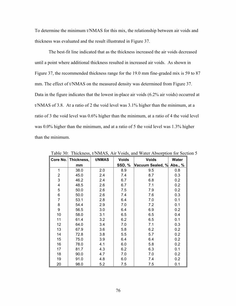
76

To determine the minimum t/NMAS for this mix, the relationship between air voids and

thickness was evaluated and the result illustrated in Figure 37.

The best-fit line indicated that as the thickness increased the air voids decreased

until a point where additional thickness resulted in increased air voids. As shown in

Figure 37, the recommended thickness range for the 19.0 mm fine-graded mix is 59 to 87

mm. The effect of t/NMAS on the measured density was determined from Figure 37.

Data in the figure indicates that the lowest in-place air voids (6.2% air voids) occurred at

t/NMAS of 3.8. At a ratio of 2 the void level was 3.1% higher than the minimum, at a

ratio of 3 the void level was 0.6% higher than the minimum, at a ratio of 4 the void level

was 0.0% higher than the minimum, and at a ratio of 5 the void level was 1.3% higher

than the minimum.



10 58.0 3.1 6.5 6.5 0.4 11 61.4 3.2 6.2 6.5 0.1 12 64.0 3.4 7.0 7.1 0.3 13 67.9 3.6 5.8 6.2 0.2 14 72.8 3.8 5.5 5.7 0.2 15 75.0 3.9 6.4 6.4 0.2 16 78.0 4.1 6.0 5.8 0.2 17 81.7 4.3 6.2 6.3 0.1 18 90.0 4.7 7.0 7.0 0.2 19 91.0 4.8 6.0 7.4 0.2 20 98.0 5.2 7.5 7.5 0.1

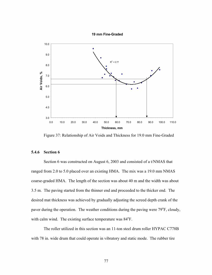
77

Figure 37: Relationship of Air Voids and Thickness for 19.0 mm Fine-Graded

5.4.6 Section 6


ranged from 2.0 to 5.0 placed over an existing HMA. The mix was a 19.0 mm NMAS

coarse-graded HMA. The length of the section was about 40 m and the width was about

3.5 m. The paving started from the thinner end and proceeded to the thicker end. The

desired mat thickness was achieved by gradually adjusting the screed depth crank of the

paver during the operation. The weather conditions during the paving were 79oF, cloudy,

with calm wind. The existing surface temperature was 84oF.


with 78 in. wide drum that could operate in vibratory and static mode. The rubber tire

19 mm Fine-Graded

R2 = 0.77

3.0

4.0

5.0

6.0

7.0

8.0

9.0

10.0

0.0 10.0 20.0 30.0 40.0 50.0 60.0 70.0 80.0 90.0 100.0 110.0

Thickness, mm

Air

Void

s, %

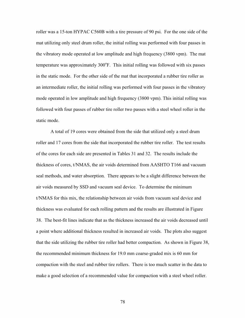
78



the vibratory mode operated at low amplitude and high frequency (3800 vpm). The mat

temperature was approximately 300oF. This initial rolling was followed with six passes

in the static mode. For the other side of the mat that incorporated a rubber tire roller as

an intermediate roller, the initial rolling was performed with four passes in the vibratory

mode operated in low amplitude and high frequency (3800 vpm). This initial rolling was

followed with four passes of rubber tire roller two passes with a steel wheel roller in the

static mode.





seal methods, and water absorption. There appears to be a slight difference between the

air voids measured by SSD and vacuum seal device. To determine the minimum

t/NMAS for this mix, the relationship between air voids from vacuum seal device and

thickness was evaluated for each rolling pattern and the results are illustrated in Figure

38. The best-fit lines indicate that as the thickness increased the air voids decreased until

a point where additional thickness resulted in increased air voids. The plots also suggest

that the side utilizing the rubber tire roller had better compaction. As shown in Figure 38,

the recommended minimum thickness for 19.0 mm coarse-graded mix is 60 mm for

compaction with the steel and rubber tire rollers. There is too much scatter in the data to

make a good selection of a recommended value for compaction with a steel wheel roller.

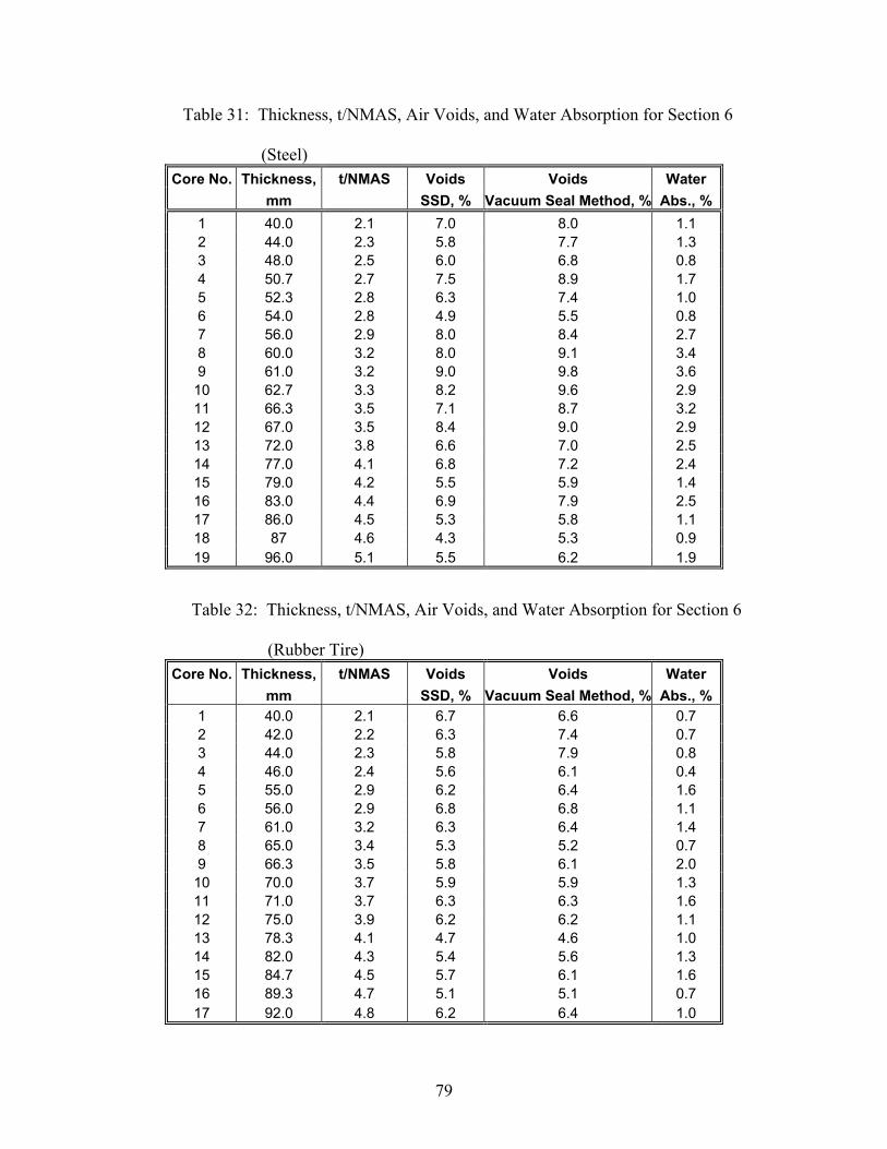
79

Table 31: Thickness, t/NMAS, Air Voids, and Water Absorption for Section 6 (Steel)

Core No. Thickness, t/NMAS Voids Voids Water mm SSD, % Vacuum Seal Method, % Abs., % 1 40.0 2.1 7.0 8.0 1.1 2 44.0 2.3 5.8 7.7 1.3 3 48.0 2.5 6.0 6.8 0.8 4 50.7 2.7 7.5 8.9 1.7 5 52.3 2.8 6.3 7.4 1.0 6 54.0 2.8 4.9 5.5 0.8 7 56.0 2.9 8.0 8.4 2.7 8 60.0 3.2 8.0 9.1 3.4 9 61.0 3.2 9.0 9.8 3.6

10 62.7 3.3 8.2 9.6 2.9 11 66.3 3.5 7.1 8.7 3.2 12 67.0 3.5 8.4 9.0 2.9 13 72.0 3.8 6.6 7.0 2.5 14 77.0 4.1 6.8 7.2 2.4 15 79.0 4.2 5.5 5.9 1.4 16 83.0 4.4 6.9 7.9 2.5 17 86.0 4.5 5.3 5.8 1.1 18 87 4.6 4.3 5.3 0.9 19 96.0 5.1 5.5 6.2 1.9


(Rubber Tire) Core No. Thickness, t/NMAS Voids Voids Water

mm SSD, % Vacuum Seal Method, % Abs., % 1 40.0 2.1 6.7 6.6 0.7 2 42.0 2.2 6.3 7.4 0.7 3 44.0 2.3 5.8 7.9 0.8 4 46.0 2.4 5.6 6.1 0.4 5 55.0 2.9 6.2 6.4 1.6 6 56.0 2.9 6.8 6.8 1.1 7 61.0 3.2 6.3 6.4 1.4 8 65.0 3.4 5.3 5.2 0.7 9 66.3 3.5 5.8 6.1 2.0

10 70.0 3.7 5.9 5.9 1.3 11 71.0 3.7 6.3 6.3 1.6 12 75.0 3.9 6.2 6.2 1.1 13 78.3 4.1 4.7 4.6 1.0 14 82.0 4.3 5.4 5.6 1.3 15 84.7 4.5 5.7 6.1 1.6 16 89.3 4.7 5.1 5.1 0.7 17 92.0 4.8 6.2 6.4 1.0

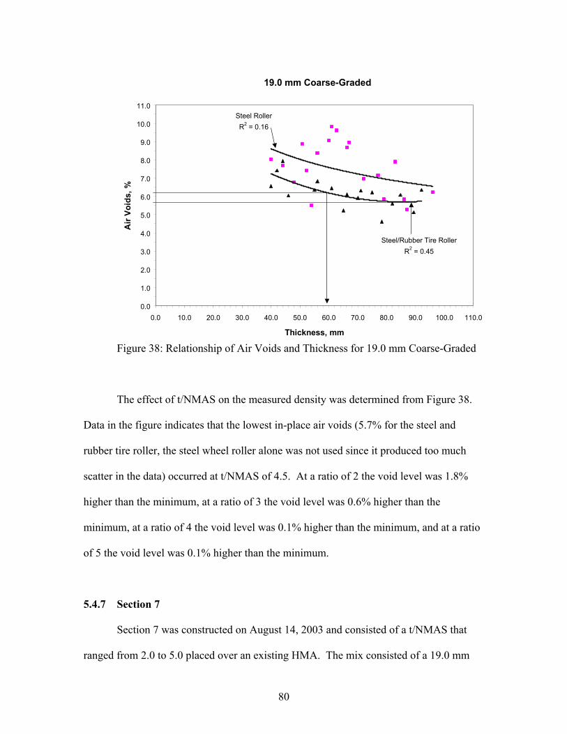
80


The effect of t/NMAS on the measured density was determined from Figure 38.

Data in the figure indicates that the lowest in-place air voids (5.7% for the steel and

rubber tire roller, the steel wheel roller alone was not used since it produced too much

scatter in the data) occurred at t/NMAS of 4.5. At a ratio of 2 the void level was 1.8%

higher than the minimum, at a ratio of 3 the void level was 0.6% higher than the

minimum, at a ratio of 4 the void level was 0.1% higher than the minimum, and at a ratio

of 5 the void level was 0.1% higher than the minimum.

5.4.7 Section 7


ranged from 2.0 to 5.0 placed over an existing HMA. The mix consisted of a 19.0 mm




0.0

1.0

2.0

3.0

4.0

5.0

6.0

7.0

8.0

9.0

10.0

11.0

0.0 10.0 20.0 30.0 40.0 50.0 60.0 70.0 80.0 90.0 100.0 110.0

Thickness, mm

Air

Void

s, %

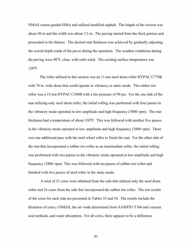
81

NMAS coarse-graded HMA and utilized modified asphalt. The length of the section was

about 40 m and the width was about 3.5 m. The paving started from the thick portion and

proceeded to the thinner. The desired mat thickness was achieved by gradually adjusting

the screed depth crank of the paver during the operation. The weather conditions during

the paving were 90oF, clear, with calm wind. The existing surface temperature was

120oF.


with 78 in. wide drum that could operate in vibratory or static mode. The rubber tire



the vibratory mode operated in low amplitude and high frequency (3800 vpm). The mat

thickness had a temperature of about 330oF. This was followed with another five passes

in the vibratory mode operated at low amplitude and high frequency (3800 vpm). There

was one additional pass with the steel wheel roller to finish the mat. For the other side of

the mat that incorporated a rubber tire roller as an intermediate roller, the initial rolling

was performed with two passes in the vibratory mode operated at low amplitude and high

frequency (3800 vpm). This was followed with ten passes of rubber tire roller and

finished with two passes of steel roller in the static mode.

A total of 23 cores were obtained from the side that utilized only the steel drum




seal methods, and water absorption. For all cores, there appears to be a difference

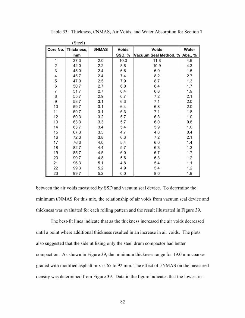
82


(Steel) Core No. Thickness, t/NMAS Voids Voids Water

mm SSD, % Vacuum Seal Method, % Abs., % 1 37.3 2.0 10.0 11.8 4.9 2 42.0 2.2 8.8 10.9 4.3 3 45.0 2.4 6.6 6.9 1.5 4 45.7 2.4 7.4 8.2 2.7 5 47.0 2.5 7.9 8.7 1.3 6 50.7 2.7 6.0 6.4 1.7 7 51.7 2.7 6.4 6.8 1.9 8 55.7 2.9 6.7 7.2 2.1 9 58.7 3.1 6.3 7.1 2.0

10 59.7 3.1 6.4 6.8 2.0 11 59.7 3.1 6.3 7.1 1.8 12 60.3 3.2 5.7 6.3 1.0 13 63.3 3.3 5.7 6.0 0.8 14 63.7 3.4 5.4 5.9 1.0 15 67.3 3.5 4.7 4.8 0.4 16 72.3 3.8 6.3 7.2 2.1 17 76.3 4.0 5.4 6.0 1.4 18 82.7 4.4 5.7 6.3 1.3 19 85.7 4.5 6.0 6.7 1.7 20 90.7 4.8 5.6 6.3 1.2 21 96.3 5.1 4.8 5.4 1.1 22 99.3 5.2 4.9 5.4 1.2 23 99.7 5.2 6.0 8.0 1.9

between the air voids measured by SSD and vacuum seal device. To determine the

minimum t/NMAS for this mix, the relationship of air voids from vacuum seal device and

thickness was evaluated for each rolling pattern and the result illustrated in Figure 39.

The best-fit lines indicate that as the thickness increased the air voids decreased

until a point where additional thickness resulted in an increase in air voids. The plots

also suggested that the side utilizing only the steel drum compactor had better

compaction. As shown in Figure 39, the minimum thickness range for 19.0 mm coarse-

graded with modified asphalt mix is 65 to 92 mm. The effect of t/NMAS on the measured

density was determined from Figure 39. Data in the figure indicates that the lowest in-

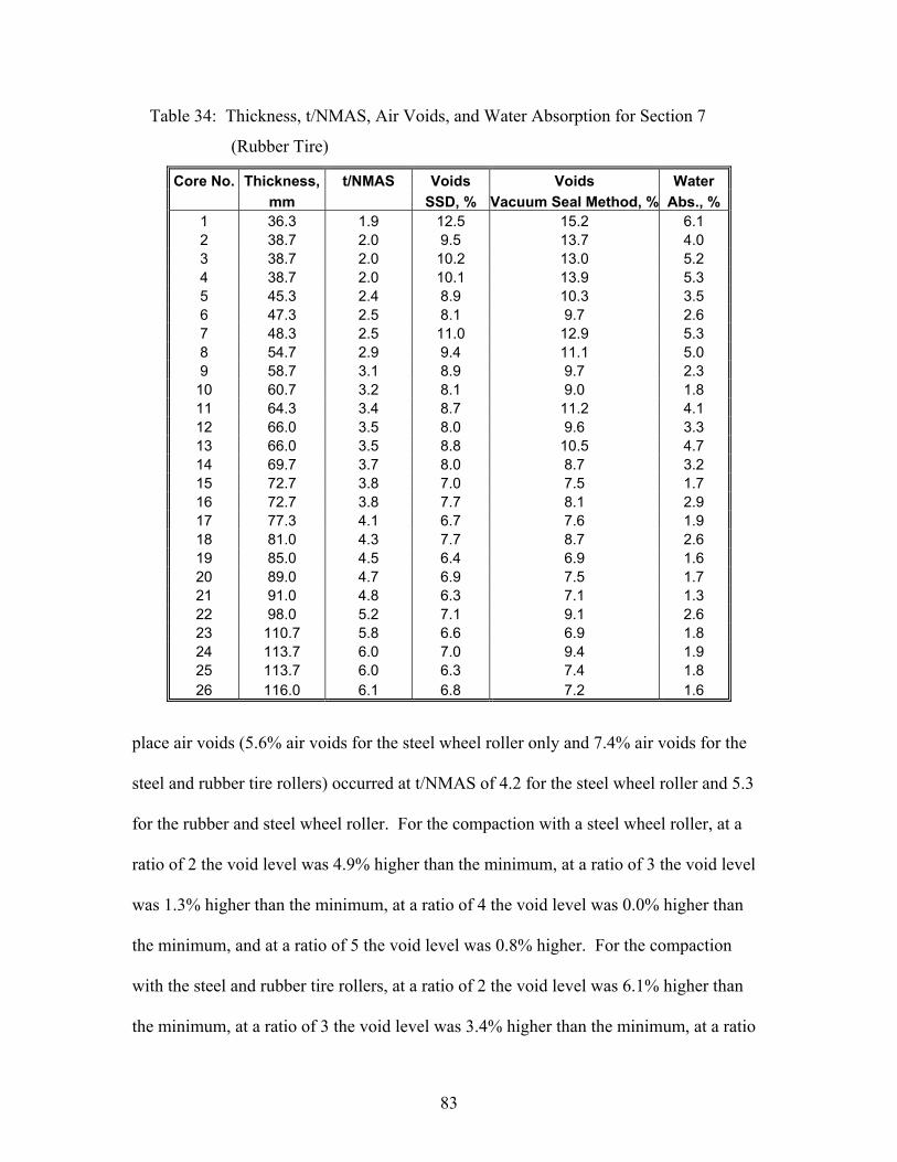
83


(Rubber Tire)

Core No. Thickness, t/NMAS Voids Voids Water mm SSD, % Vacuum Seal Method, % Abs., % 1 36.3 1.9 12.5 15.2 6.1 2 38.7 2.0 9.5 13.7 4.0 3 38.7 2.0 10.2 13.0 5.2 4 38.7 2.0 10.1 13.9 5.3 5 45.3 2.4 8.9 10.3 3.5 6 47.3 2.5 8.1 9.7 2.6 7 48.3 2.5 11.0 12.9 5.3 8 54.7 2.9 9.4 11.1 5.0 9 58.7 3.1 8.9 9.7 2.3

10 60.7 3.2 8.1 9.0 1.8 11 64.3 3.4 8.7 11.2 4.1 12 66.0 3.5 8.0 9.6 3.3 13 66.0 3.5 8.8 10.5 4.7 14 69.7 3.7 8.0 8.7 3.2 15 72.7 3.8 7.0 7.5 1.7 16 72.7 3.8 7.7 8.1 2.9 17 77.3 4.1 6.7 7.6 1.9 18 81.0 4.3 7.7 8.7 2.6 19 85.0 4.5 6.4 6.9 1.6 20 89.0 4.7 6.9 7.5 1.7 21 91.0 4.8 6.3 7.1 1.3 22 98.0 5.2 7.1 9.1 2.6 23 110.7 5.8 6.6 6.9 1.8 24 113.7 6.0 7.0 9.4 1.9 25 113.7 6.0 6.3 7.4 1.8 26 116.0 6.1 6.8 7.2 1.6

place air voids (5.6% air voids for the steel wheel roller only and 7.4% air voids for the

steel and rubber tire rollers) occurred at t/NMAS of 4.2 for the steel wheel roller and 5.3

for the rubber and steel wheel roller. For the compaction with a steel wheel roller, at a

ratio of 2 the void level was 4.9% higher than the minimum, at a ratio of 3 the void level

was 1.3% higher than the minimum, at a ratio of 4 the void level was 0.0% higher than

the minimum, and at a ratio of 5 the void level was 0.8% higher. For the compaction

with the steel and rubber tire rollers, at a ratio of 2 the void level was 6.1% higher than

the minimum, at a ratio of 3 the void level was 3.4% higher than the minimum, at a ratio

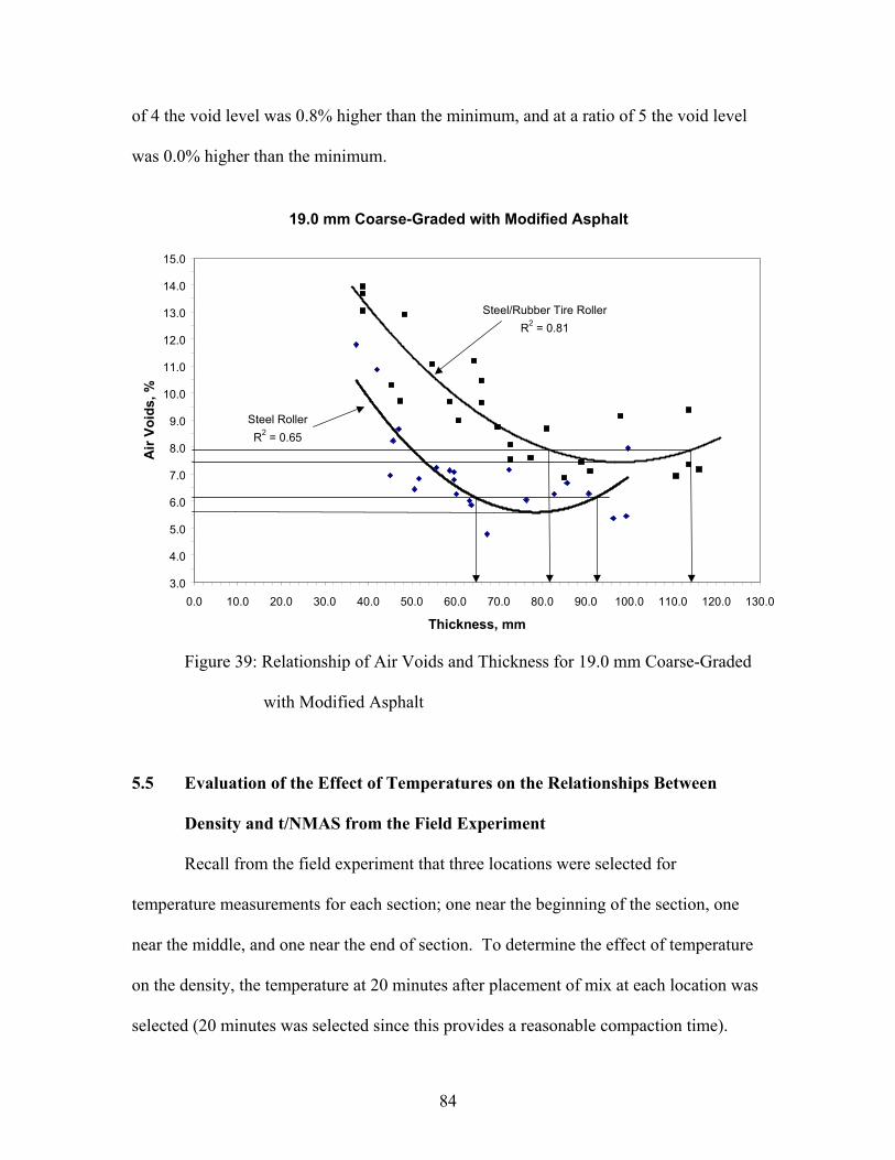
84

of 4 the void level was 0.8% higher than the minimum, and at a ratio of 5 the void level

was 0.0% higher than the minimum.


with Modified Asphalt

5.5 Evaluation of the Effect of Temperatures on the Relationships Between

Density and t/NMAS from the Field Experiment

Recall from the field experiment that three locations were selected for

temperature measurements for each section; one near the beginning of the section, one

near the middle, and one near the end of section. To determine the effect of temperature

on the density, the temperature at 20 minutes after placement of mix at each location was

selected (20 minutes was selected since this provides a reasonable compaction time).

19.0 mm Coarse-Graded with Modified Asphalt



3.0

4.0

5.0

6.0

7.0

8.0

9.0

10.0

11.0

12.0

13.0

14.0

15.0

0.0 10.0 20.0 30.0 40.0 50.0 60.0 70.0 80.0 90.0 100.0 110.0 120.0 130.0

Thickness, mm

Air

Void

s, %

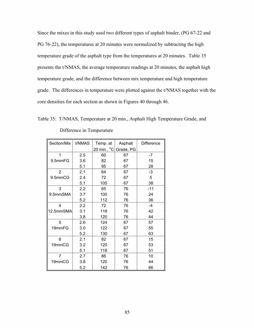
85

Since the mixes in this study used two different types of asphalt binder, (PG 67-22 and

PG 76-22), the temperatures at 20 minutes were normalized by subtracting the high

temperature grade of the asphalt type from the temperatures at 20 minutes. Table 35

presents the t/NMAS, the average temperature readings at 20 minutes, the asphalt high

temperature grade, and the difference between mix temperature and high temperature

grade. The differences in temperature were plotted against the t/NMAS together with the

core densities for each section as shown in Figures 40 through 46.

Table 35: T/NMAS, Temperature at 20 min., Asphalt High Temperature Grade, and

Difference in Temperature

Section/Mix t/NMAS Temp. at Asphalt Difference 20 min., oC Grade, PG 1 2.5 60 67 -7

9.5mmFG 3.6 82 67 15 5.1 95 67 28 2 2.1 64 67 -3

9.5mmCG 2.4 72 67 5 5.1 105 67 38 3 2.2 65 76 -11

9.5mmSMA 3.7 100 76 24 5.2 112 76 36 4 2.2 72 76 -4

12.5mmSMA 3.1 118 76 42 3.8 120 76 44 5 2.6 124 67 57

19mmFG 3.0 122 67 55 5.2 130 67 63 6 2.1 82 67 15

19mmCG 3.2 120 67 53 5.1 118 67 51 7 2.7 86 76 10

19mmCG 3.8 120 76 44 5.2 142 76 66

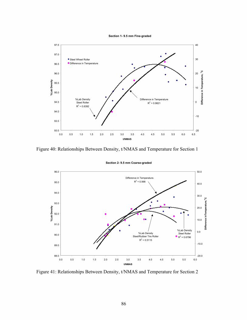
86

Figure 40: Relationships Between Density, t/NMAS and Temperature for Section 1


Section 1- 9.5 mm Fine-graded

%Lab DensitySteel RollerR2 = 0.6392

Difference in Temperature R2 = 0.9821

93.0

93.5

94.0

94.5

95.0

95.5

96.0

96.5

97.0

97.5

0.0 0.5 1.0 1.5 2.0 2.5 3.0 3.5 4.0 4.5 5.0 5.5 6.0 6.5

t/NMAS

%La

b D

ensi

ty

-20

-10

0

10

20

30

40

Diff

eren

ce in

Tem

pera

ture

, o C

Steel Wheel RollerDifference in Temperature

Section 2- 9.5 mm Coarse-graded

Difference in Temperature.R2 = 0.998


%Lab DensitySteel/Rubber Tire Roller

R2 = 0.5115

88.0

89.0

90.0

91.0

92.0

93.0

94.0

95.0

96.0

0.0 0.5 1.0 1.5 2.0 2.5 3.0 3.5 4.0 4.5 5.0 5.5 6.0

t/NMAS

%La

b D

ensi

ty

-20.0

-10.0

0.0

10.0

20.0

30.0

40.0

50.0

Diff

eren

ce in

Tem

pera

ture

,o C

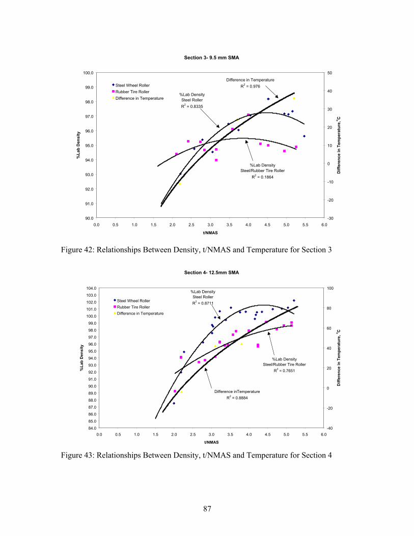
87



Section 3- 9.5 mm SMA

Difference in TemperatureR2 = 0.976



R2 = 0.1864

90.0

91.0

92.0

93.0

94.0

95.0

96.0

97.0

98.0

99.0

100.0

0.0 0.5 1.0 1.5 2.0 2.5 3.0 3.5 4.0 4.5 5.0 5.5 6.0

t/NMAS

%La

b D

ensi

ty

-30

-20

-10

0

10

20

30

40

50

Diff

eren

ce in

Tem

pera

ture

,o C

Steel Wheel RollerRubber Tire RollerDifference in Temperature

Section 4- 12.5mm SMA

Difference inTemperatureR2 = 0.8884



R2 = 0.7651

84.0

85.0

86.0

87.0

88.0

89.0

90.0

91.0

92.0

93.0

94.0

95.0

96.0

97.0

98.0

99.0

100.0

101.0

102.0

103.0

104.0

0.0 0.5 1.0 1.5 2.0 2.5 3.0 3.5 4.0 4.5 5.0 5.5 6.0

t/NMAS

%La

b D

ensi

ty

-40

-20

0

20

40

60

80

100

Diff

eren

ce in

Tem

pera

ture

, o C

Steel Wheel RollerRubber Tire RollerDifference in Temperature

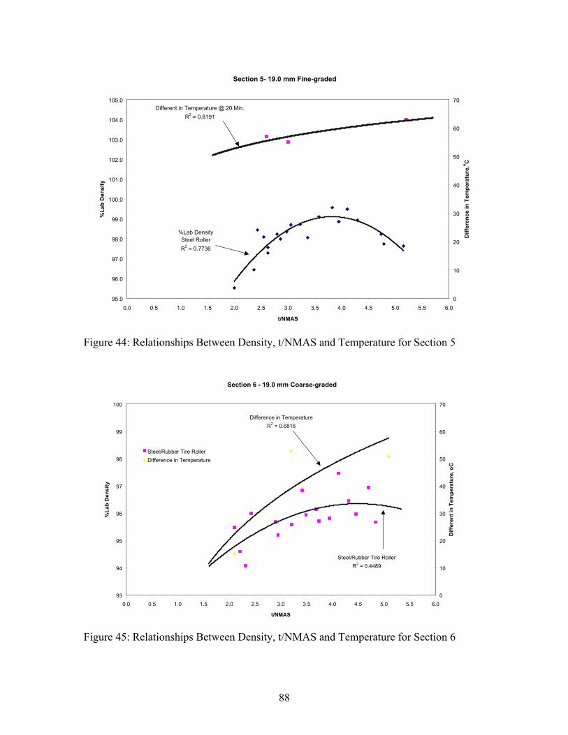
88



Section 5- 19.0 mm Fine-graded


Different in Temperature @ 20 Min.R2 = 0.8191

95.0

96.0

97.0

98.0

99.0

100.0

101.0

102.0

103.0

104.0

105.0

0.0 0.5 1.0 1.5 2.0 2.5 3.0 3.5 4.0 4.5 5.0 5.5 6.0

t/NMAS

%La

b D

ensi

ty

0

10

20

30

40

50

60

70

Diff

eren

ce in

Tem

pera

ture

,o C

Section 6 - 19.0 mm Coarse-graded

Difference in Temperature R2 = 0.6816


93

94

95

96

97

98

99

100

0.0 0.5 1.0 1.5 2.0 2.5 3.0 3.5 4.0 4.5 5.0 5.5 6.0

t/NMAS

%La

b D

ensi

ty

0

10

20

30

40

50

60

70

Diff

eren

t in

Tem

pera

ture

, oC

Steel/Rubber Tire RollerDifference in Temperature

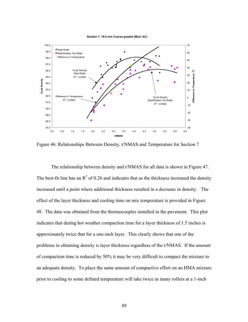
89


The relationship between density and t/NMAS for all data is shown in Figure 47.

The best-fit line has an R2 of 0.26 and indicates that as the thickness increased the density

increased until a point where additional thickness resulted in a decrease in density. The

effect of the layer thickness and cooling time on mix temperature is provided in Figure

48. The data was obtained from the thermocouples installed in the pavement. This plot

indicates that during hot weather compaction time for a layer thickness of 1.5 inches is

approximately twice that for a one-inch layer. This clearly shows that one of the

problems in obtaining density is layer thickness regardless of the t/NMAS. If the amount

of compaction time is reduced by 50% it may be very difficult to compact the mixture to

an adequate density. To place the same amount of compactive effort on an HMA mixture

prior to cooling to some defined temperature will take twice as many rollers at a 1-inch

Section 7- 19.0 mm Coarse-graded (Mod. AC)

Difference in TemperatureR2 = 0.9904



R2 = 0.8092

87.0

88.0

89.0

90.0

91.0

92.0

93.0

94.0

95.0

96.0

97.0

98.0

99.0

100.0

0.0 0.5 1.0 1.5 2.0 2.5 3.0 3.5 4.0 4.5 5.0 5.5 6.0 6.5

t/NMAS

%La

b D

ensi

ty

-40

-30

-20

-10

0

10

20

30

40

50

60

70

Diff

eren

ce in

Tem

pera

ture

, o C

Steel RollerSteel/Rubber Tire RollerDifference in Temperature

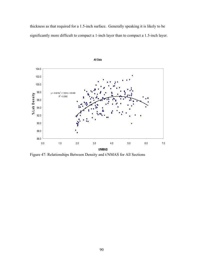
90

thickness as that required for a 1.5-inch surface. Generally speaking it is likely to be

significantly more difficult to compact a 1-inch layer than to compact a 1.5-inch layer.

Figure 47: Relationships Between Density and t/NMAS for All Sections

All Data

y = -0.8216x2 + 7.2531x + 80.848R2 = 0.2562

86.0

88.0

90.0

92.0

94.0

96.0

98.0

100.0

102.0

104.0

0.0 1.0 2.0 3.0 4.0 5.0 6.0 7.0

t/NMAS

%La

b D

ensi

ty

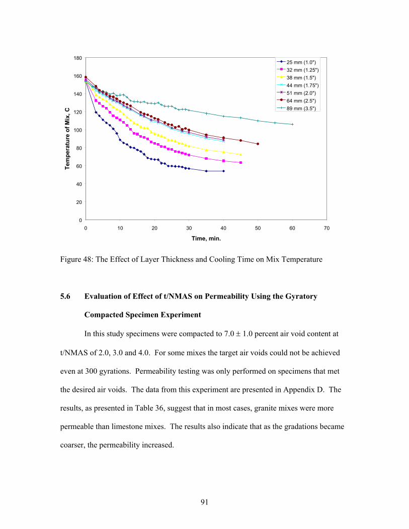
91

0

20

40

60

80

100

120

140

160

180

0 10 20 30 40 50 60 70

Time, min.

Tem

pera

ture

of M

ix, C

25 mm (1.0")32 mm (1.25")38 mm (1.5")44 mm (1.75")51 mm (2.0")64 mm (2.5")89 mm (3.5")

Figure 48: The Effect of Layer Thickness and Cooling Time on Mix Temperature

5.6 Evaluation of Effect of t/NMAS on Permeability Using the Gyratory

Compacted Specimen Experiment

In this study specimens were compacted to 7.0 ± 1.0 percent air void content at

t/NMAS of 2.0, 3.0 and 4.0. For some mixes the target air voids could not be achieved

even at 300 gyrations. Permeability testing was only performed on specimens that met

the desired air voids. The data from this experiment are presented in Appendix D. The

results, as presented in Table 36, suggest that in most cases, granite mixes were more

permeable than limestone mixes. The results also indicate that as the gradations became

coarser, the permeability increased.

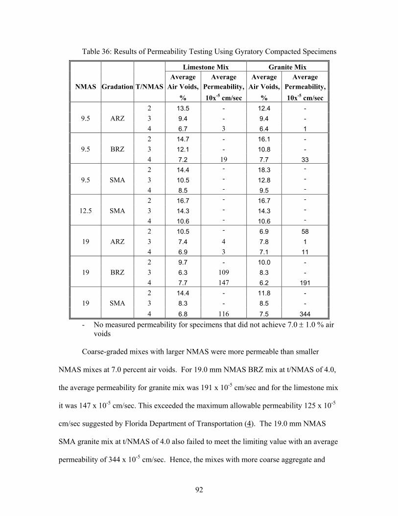
92

Table 36: Results of Permeability Testing Using Gyratory Compacted Specimens

Limestone Mix Granite Mix Average Average Average Average

NMAS Gradation T/NMAS Air Voids, Permeability, Air Voids, Permeability, % 10x-5 cm/sec % 10x-5 cm/sec 2 13.5 - 12.4 -

9.5 ARZ 3 9.4 - 9.4 - 4 6.7 3 6.4 1 2 14.7 - 16.1 -

9.5 BRZ 3 12.1 - 10.8 - 4 7.2 19 7.7 33 2 14.4 - 18.3 -

9.5 SMA 3 10.5 - 12.8 -

4 8.5 - 9.5 -

2 16.7 - 16.7 -

12.5 SMA 3 14.3 - 14.3 -

4 10.6 - 10.6 -

2 10.5 - 6.9 58 19 ARZ 3 7.4 4 7.8 1 4 6.9 3 7.1 11 2 9.7 - 10.0 -

19 BRZ 3 6.3 109 8.3 - 4 7.7 147 6.2 191 2 14.4 - 11.8 -

19 SMA 3 8.3 - 8.5 - 4 6.8 116 7.5 344

- No measured permeability for specimens that did not achieve 7.0 ± 1.0 % air voids

Coarse-graded mixes with larger NMAS were more permeable than smaller

NMAS mixes at 7.0 percent air voids. For 19.0 mm NMAS BRZ mix at t/NMAS of 4.0,

the average permeability for granite mix was 191 x 10-5 cm/sec and for the limestone mix

it was 147 x 10-5 cm/sec. This exceeded the maximum allowable permeability 125 x 10-5

cm/sec suggested by Florida Department of Transportation (4). The 19.0 mm NMAS

SMA granite mix at t/NMAS of 4.0 also failed to meet the limiting value with an average

permeability of 344 x 10-5 cm/sec. Hence, the mixes with more coarse aggregate and

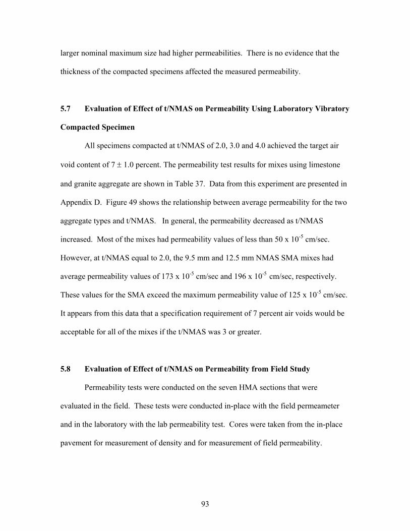
93

larger nominal maximum size had higher permeabilities. There is no evidence that the

thickness of the compacted specimens affected the measured permeability.

5.7 Evaluation of Effect of t/NMAS on Permeability Using Laboratory Vibratory

Compacted Specimen

All specimens compacted at t/NMAS of 2.0, 3.0 and 4.0 achieved the target air

void content of 7 ± 1.0 percent. The permeability test results for mixes using limestone

and granite aggregate are shown in Table 37. Data from this experiment are presented in

Appendix D. Figure 49 shows the relationship between average permeability for the two

aggregate types and t/NMAS. In general, the permeability decreased as t/NMAS

increased. Most of the mixes had permeability values of less than 50 x 10-5 cm/sec.

However, at t/NMAS equal to 2.0, the 9.5 mm and 12.5 mm NMAS SMA mixes had

average permeability values of 173 x 10-5 cm/sec and 196 x 10-5 cm/sec, respectively.

These values for the SMA exceed the maximum permeability value of 125 x 10-5 cm/sec.

It appears from this data that a specification requirement of 7 percent air voids would be

acceptable for all of the mixes if the t/NMAS was 3 or greater.

5.8 Evaluation of Effect of t/NMAS on Permeability from Field Study

Permeability tests were conducted on the seven HMA sections that were

evaluated in the field. These tests were conducted in-place with the field permeameter

and in the laboratory with the lab permeability test. Cores were taken from the in-place

pavement for measurement of density and for measurement of field permeability.

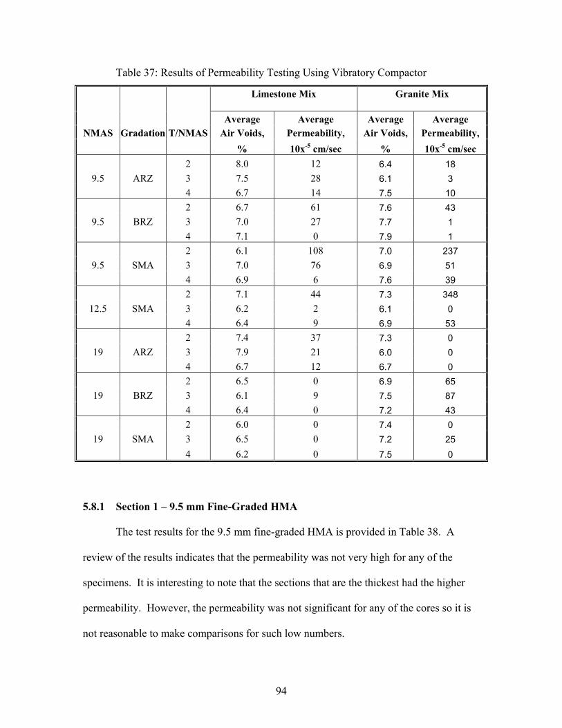
94

Table 37: Results of Permeability Testing Using Vibratory Compactor

Limestone Mix

Granite Mix

Average Average Average Average

NMAS Gradation T/NMAS Air Voids, Permeability, Air Voids, Permeability, % 10x-5 cm/sec % 10x-5 cm/sec 2 8.0 12 6.4 18

9.5 ARZ 3 7.5 28 6.1 3 4 6.7 14 7.5 10 2 6.7 61 7.6 43

9.5 BRZ 3 7.0 27 7.7 1 4 7.1 0 7.9 1 2 6.1 108 7.0 237

9.5 SMA 3 7.0 76 6.9 51 4 6.9 6 7.6 39 2 7.1 44 7.3 348

12.5 SMA 3 6.2 2 6.1 0 4 6.4 9 6.9 53 2 7.4 37 7.3 0

19 ARZ 3 7.9 21 6.0 0 4 6.7 12 6.7 0 2 6.5 0 6.9 65

19 BRZ 3 6.1 9 7.5 87 4 6.4 0 7.2 43 2 6.0 0 7.4 0

19 SMA 3 6.5 0 7.2 25 4 6.2 0 7.5 0

5.8.1 Section 1 – 9.5 mm Fine-Graded HMA

The test results for the 9.5 mm fine-graded HMA is provided in Table 38. A

review of the results indicates that the permeability was not very high for any of the

specimens. It is interesting to note that the sections that are the thickest had the higher

permeability. However, the permeability was not significant for any of the cores so it is

not reasonable to make comparisons for such low numbers.

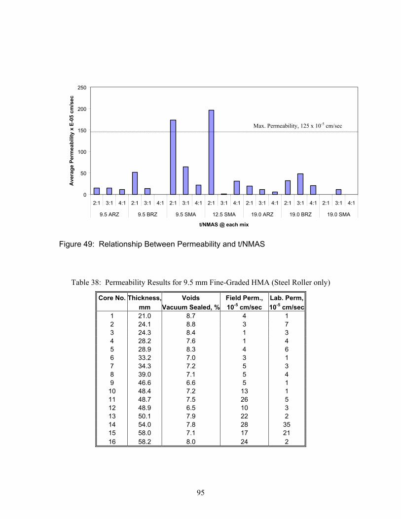
95

0

50

100

150

200

250

2:1 3:1 4:1 2:1 3:1 4:1 2:1 3:1 4:1 2:1 3:1 4:1 2:1 3:1 4:1 2:1 3:1 4:1 2:1 3:1 4:1

9.5 ARZ 9.5 BRZ 9.5 SMA 12.5 SMA 19.0 ARZ 19.0 BRZ 19.0 SMA

t/NMAS @ each mix

Ave

rage

Per

mea

bilit

y x

E-05

cm

/sec

Figure 49: Relationship Between Permeability and t/NMAS

Table 38: Permeability Results for 9.5 mm Fine-Graded HMA (Steel Roller only)

Core No. Thickness, Voids Field Perm., Lab. Perm, mm Vacuum Sealed, % 10-5 cm/sec 10-5 cm/sec 1 21.0 8.7 4 1 2 24.1 8.8 3 7 3 24.3 8.4 1 3 4 28.2 7.6 1 4 5 28.9 8.3 4 6 6 33.2 7.0 3 1 7 34.3 7.2 5 3 8 39.0 7.1 5 4 9 46.6 6.6 5 1

10 48.4 7.2 13 1 11 48.7 7.5 26 5 12 48.9 6.5 10 3 13 50.1 7.9 22 2 14 54.0 7.8 28 35 15 58.0 7.1 17 21 16 58.2 8.0 24 2

Max. Permeability, 125 x 10-5 cm/sec

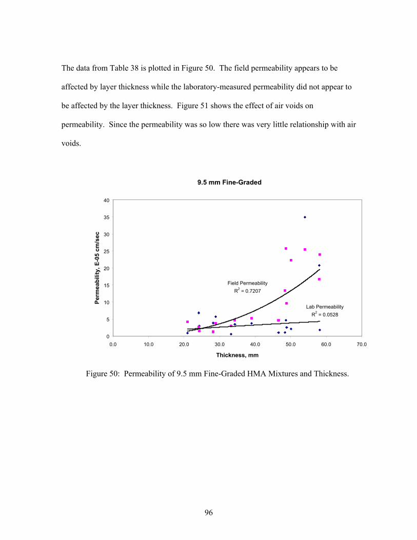
96

The data from Table 38 is plotted in Figure 50. The field permeability appears to be

affected by layer thickness while the laboratory-measured permeability did not appear to

be affected by the layer thickness. Figure 51 shows the effect of air voids on

permeability. Since the permeability was so low there was very little relationship with air

voids.

Figure 50: Permeability of 9.5 mm Fine-Graded HMA Mixtures and Thickness.

9.5 mm Fine-Graded

Field PermeabilityR2 = 0.7207

Lab PermeabilityR2 = 0.0528

0

5

10

15

20

25

30

35

40

0.0 10.0 20.0 30.0 40.0 50.0 60.0 70.0

Thickness, mm

Perm

eabi

lity,

E-0

5 cm

/sec

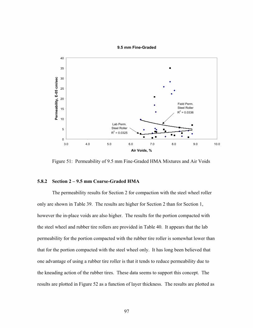
97

Figure 51: Permeability of 9.5 mm Fine-Graded HMA Mixtures and Air Voids

5.8.2 Section 2 – 9.5 mm Coarse-Graded HMA

The permeability results for Section 2 for compaction with the steel wheel roller

only are shown in Table 39. The results are higher for Section 2 than for Section 1,

however the in-place voids are also higher. The results for the portion compacted with

the steel wheel and rubber tire rollers are provided in Table 40. It appears that the lab

permeability for the portion compacted with the rubber tire roller is somewhat lower than

that for the portion compacted with the steel wheel only. It has long been believed that

one advantage of using a rubber tire roller is that it tends to reduce permeability due to

the kneading action of the rubber tires. These data seems to support this concept. The

results are plotted in Figure 52 as a function of layer thickness. The results are plotted as

9.5 mm Fine-Graded

Lab Perm.Steel RollerR2 = 0.0325

Field Perm.Steel RollerR2 = 0.0336

0

5

10

15

20

25

30

35

40

3.0 4.0 5.0 6.0 7.0 8.0 9.0 10.0

Air Voids, %

Perm

eabi

lity,

E-0

5 cm

/sec

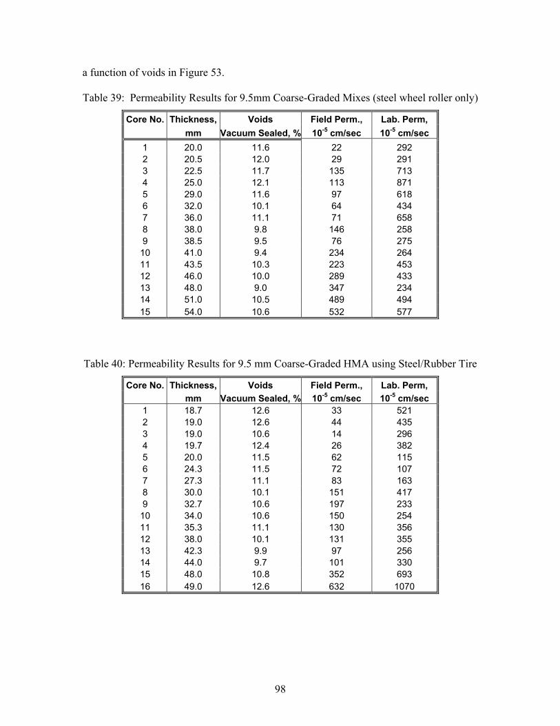
98

a function of voids in Figure 53.

Table 39: Permeability Results for 9.5mm Coarse-Graded Mixes (steel wheel roller only)


10 41.0 9.4 234 264 11 43.5 10.3 223 453 12 46.0 10.0 289 433 13 48.0 9.0 347 234 14 51.0 10.5 489 494 15 54.0 10.6 532 577

Table 40: Permeability Results for 9.5 mm Coarse-Graded HMA using Steel/Rubber Tire


10 34.0 10.6 150 254 11 35.3 11.1 130 356 12 38.0 10.1 131 355 13 42.3 9.9 97 256 14 44.0 9.7 101 330 15 48.0 10.8 352 693 16 49.0 12.6 632 1070

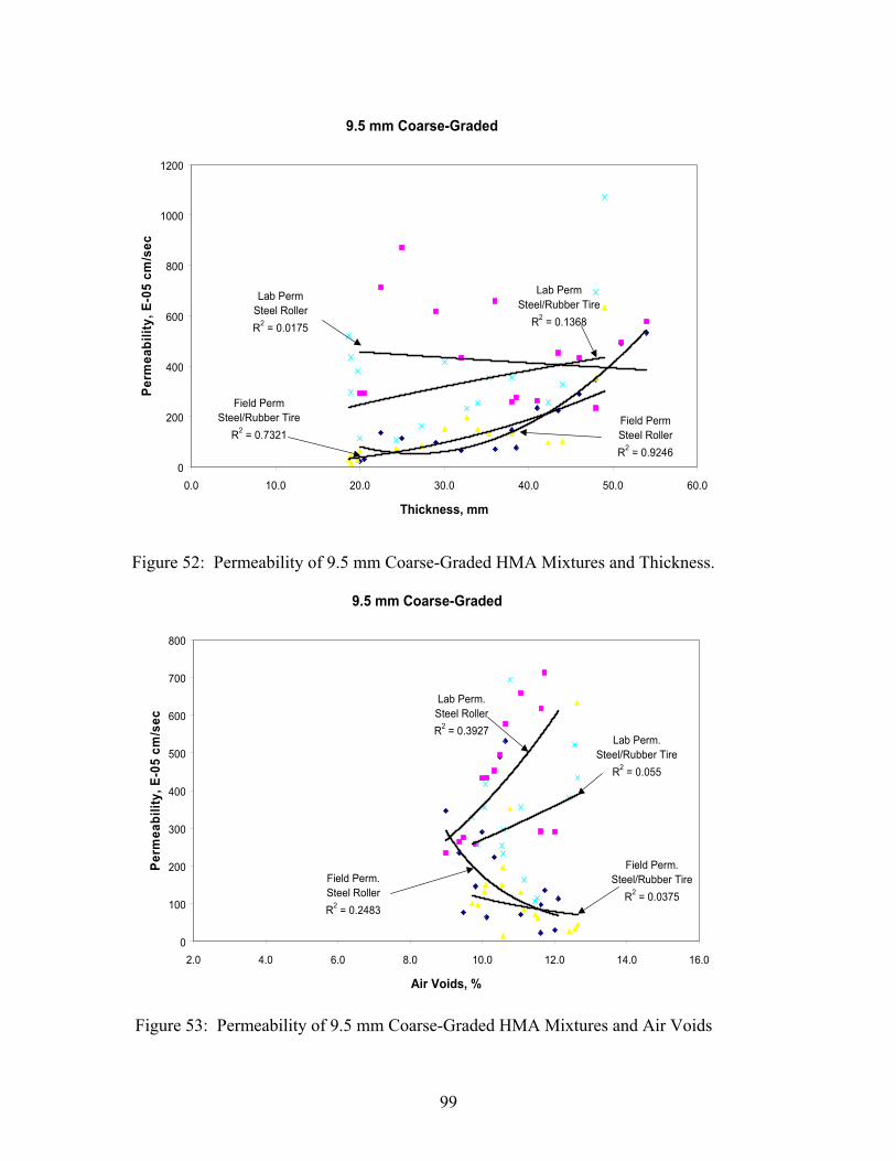
99

Figure 52: Permeability of 9.5 mm Coarse-Graded HMA Mixtures and Thickness.


Field PermSteel RollerR2 = 0.9246

Lab PermSteel RollerR2 = 0.0175

Field PermSteel/Rubber Tire

R2 = 0.7321

Lab PermSteel/Rubber Tire

R2 = 0.1368

0

200

400

600

800

1000

1200

0.0 10.0 20.0 30.0 40.0 50.0 60.0

Thickness, mm

Perm

eabi

lity,

E-0

5 cm

/se c




Field Perm.Steel/Rubber Tire

R2 = 0.0375

Lab Perm.Steel/Rubber Tire

R2 = 0.055

0

100

200

300

400

500

600

700

800

2.0 4.0 6.0 8.0 10.0 12.0 14.0 16.0

Air Voids, %

Perm

eabi

lity,

E-0

5 cm

/se c

Figure 53: Permeability of 9.5 mm Coarse-Graded HMA Mixtures and Air Voids

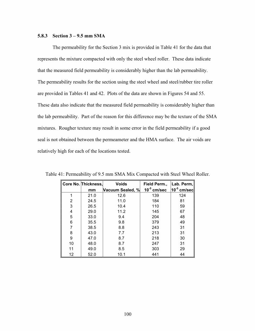
100

5.8.3 Section 3 – 9.5 mm SMA

The permeability for the Section 3 mix is provided in Table 41 for the data that

represents the mixture compacted with only the steel wheel roller. These data indicate

that the measured field permeability is considerably higher than the lab permeability.

The permeability results for the section using the steel wheel and steel/rubber tire roller

are provided in Tables 41 and 42. Plots of the data are shown in Figures 54 and 55.

These data also indicate that the measured field permeability is considerably higher than

the lab permeability. Part of the reason for this difference may be the texture of the SMA

mixtures. Rougher texture may result in some error in the field permeability if a good

seal is not obtained between the permeameter and the HMA surface. The air voids are

relatively high for each of the locations tested.

Table 41: Permeability of 9.5 mm SMA Mix Compacted with Steel Wheel Roller.


10 48.0 8.7 247 31 11 49.0 8.5 303 29 12 52.0 10.1 441 44

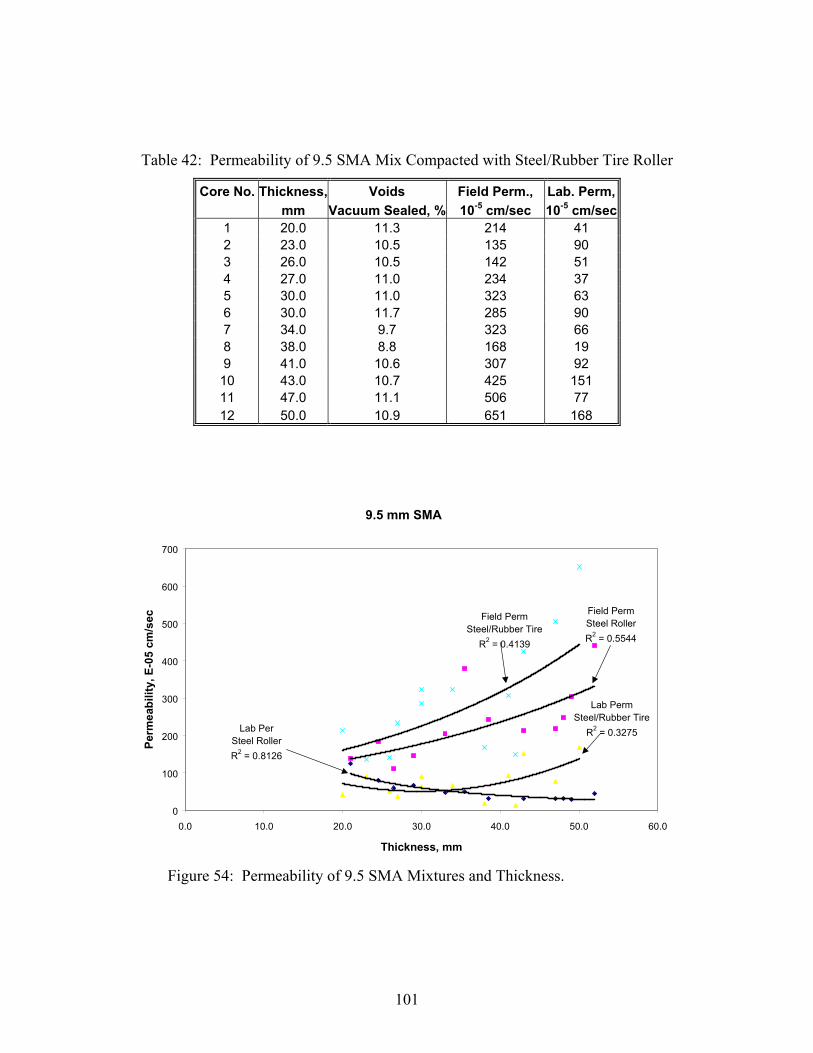
101

Table 42: Permeability of 9.5 SMA Mix Compacted with Steel/Rubber Tire Roller


10 43.0 10.7 425 151 11 47.0 11.1 506 77 12 50.0 10.9 651 168

Figure 54: Permeability of 9.5 SMA Mixtures and Thickness.

9.5 mm SMA


Lab PerSteel RollerR2 = 0.8126


R2 = 0.3275


R2 = 0.4139

0

100

200

300

400

500

600

700

0.0 10.0 20.0 30.0 40.0 50.0 60.0

Thickness, mm

Perm

eabi

lity,

E-0

5 cm

/sec

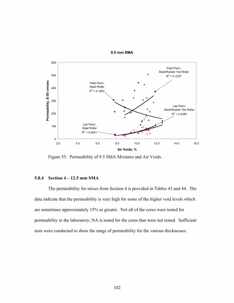
102

Figure 55: Permeability of 9.5 SMA Mixtures and Air Voids.

5.8.4 Section 4 – 12.5 mm SMA

The permeability for mixes from Section 4 is provided in Tables 43 and 44. The

data indicate that the permeability is very high for some of the higher void levels which

are sometimes approximately 15% or greater. Not all of the cores were tested for

permeability in the laboratory; NA is noted for the cores that were not tested. Sufficient

tests were conducted to show the range of permeability for the various thicknesses.

9.5 mm SMA



Lab Perm.Steel/Rubber Tire Roller

R2 = 0.2385

Field Perm.Steel/Rubber Tire Roller

R2 = 0.1037

0

100

200

300

400

500

600

2.0 4.0 6.0 8.0 10.0 12.0 14.0 16.0

Air Voids, %

Perm

eabi

lity,

E-0

5 cm

/sec

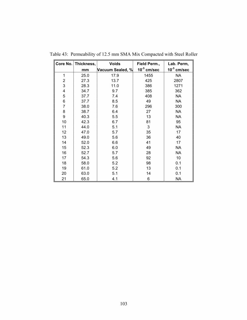
103

Table 43: Permeability of 12.5 mm SMA Mix Compacted with Steel Roller

Core No. Thickness, Voids Field Perm., Lab. Perm, mm Vacuum Sealed, % 10-5 cm/sec 10-5 cm/sec 1 25.0 17.9 1455 NA 2 27.3 13.7 425 2807 3 28.3 11.0 386 1271 4 34.7 9.7 385 362 5 37.7 7.4 408 NA 6 37.7 8.5 49 NA 7 38.0 7.6 296 300 8 38.7 6.4 27 NA 9 40.3 5.5 13 NA

10 42.3 6.7 81 95 11 44.0 5.1 3 NA 12 47.0 5.7 35 17 13 49.0 5.6 36 40 14 52.0 6.6 41 17 15 52.3 6.0 49 NA 16 52.7 5.7 28 NA 17 54.3 5.6 92 10 18 58.0 5.2 98 0.1 19 61.0 5.2 13 0.1 20 63.0 5.1 14 0.1 21 65.0 4.1 6 NA

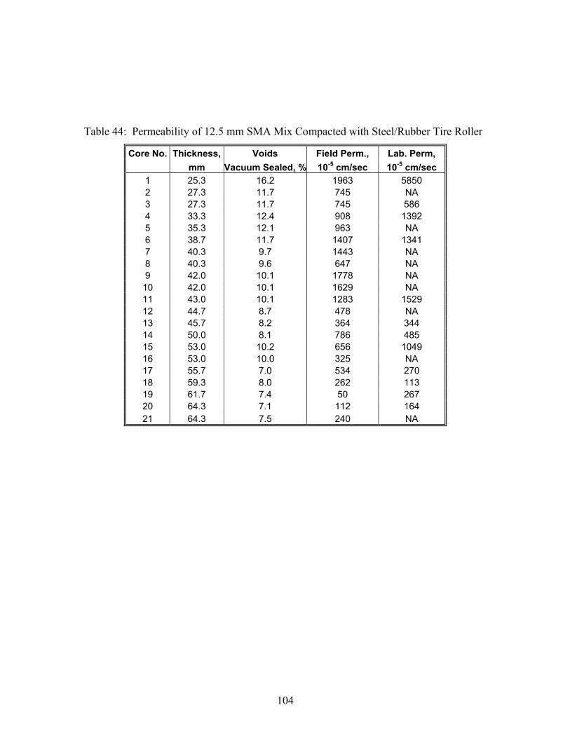
104

Table 44: Permeability of 12.5 mm SMA Mix Compacted with Steel/Rubber Tire Roller

Core No. Thickness, Voids Field Perm., Lab. Perm, mm Vacuum Sealed, % 10-5 cm/sec 10-5 cm/sec 1 25.3 16.2 1963 5850 2 27.3 11.7 745 NA 3 27.3 11.7 745 586 4 33.3 12.4 908 1392 5 35.3 12.1 963 NA 6 38.7 11.7 1407 1341 7 40.3 9.7 1443 NA 8 40.3 9.6 647 NA 9 42.0 10.1 1778 NA

10 42.0 10.1 1629 NA 11 43.0 10.1 1283 1529 12 44.7 8.7 478 NA 13 45.7 8.2 364 344 14 50.0 8.1 786 485 15 53.0 10.2 656 1049 16 53.0 10.0 325 NA 17 55.7 7.0 534 270 18 59.3 8.0 262 113 19 61.7 7.4 50 267 20 64.3 7.1 112 164 21 64.3 7.5 240 NA

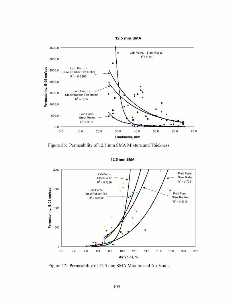
105

Figure 56: Permeability of 12.5 mm SMA Mixture and Thickness.

12.5 mm SMA

Field Perm. Steel Roller

R2 = 0.51

Lab Perm. - Steel RollerR2 = 0.85

Field Perm. - Steel/Rubber Tire Roller

R2 = 0.55

Lab. Perm. - Steel/Rubber Tire Roller

R2 = 0.6296

0.0

500.0

1000.0

1500.0

2000.0

2500.0

3000.0

3500.0

0.0 10.0 20.0 30.0 40.0 50.0 60.0 70.0

Thickness, mm

Perm

eabi

lity,

E-0

5 cm

/sec

12.5 mm SMA



Lab Perm.Steel/Rubber Tire

R2 = 0.8092Field Perm.

Steel/RubberR2 = 0.4919

0

500

1000

1500

2000

0.0 2.0 4.0 6.0 8.0 10.0 12.0 14.0 16.0 18.0 20.0 22.0

Air Voids, %

Perm

eabi

lity,

E-0

5 cm

/sec

Figure 57: Permeability of 12.5 mm SMA Mixture and Air Voids

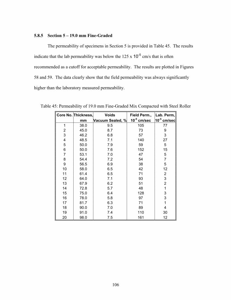
106

5.8.5 Section 5 – 19.0 mm Fine-Graded

The permeability of specimens in Section 5 is provided in Table 45. The results

indicate that the lab permeability was below the 125 x 10-5 cm/s that is often

recommended as a cutoff for acceptable permeability. The results are plotted in Figures

58 and 59. The data clearly show that the field permeability was always significantly

higher than the laboratory measured permeability.

Table 45: Permeability of 19.0 mm Fine-Graded Mix Compacted with Steel Roller


10 58.0 6.5 42 12 11 61.4 6.5 71 2 12 64.0 7.1 93 3 13 67.9 6.2 51 2 14 72.8 5.7 48 1 15 75.0 6.4 128 3 16 78.0 5.8 97 3 17 81.7 6.3 71 1 18 90.0 7.0 89 4 19 91.0 7.4 110 30 20 98.0 7.5 161 12

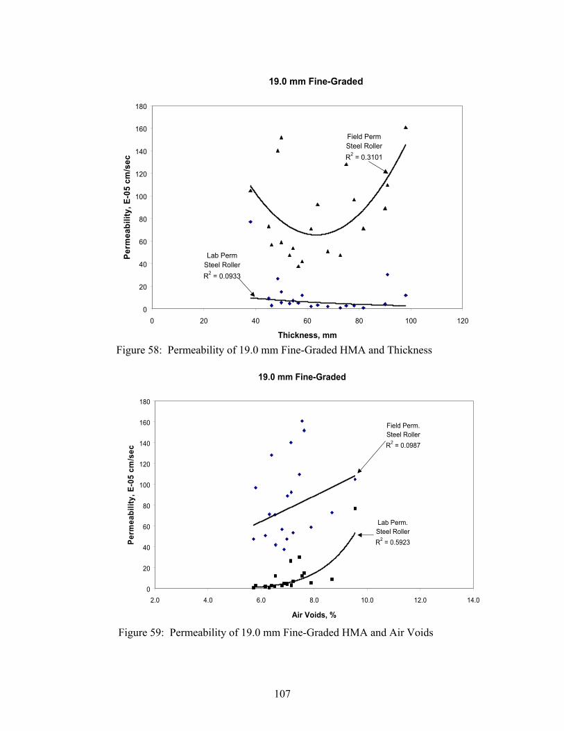
107

Figure 58: Permeability of 19.0 mm Fine-Graded HMA and Thickness

19.0 mm Fine-Graded



0

20

40

60

80

100

120

140

160

180

0 20 40 60 80 100 120

Thickness, mm

Perm

eabi

lity,

E-0

5 cm

/sec

19.0 mm Fine-Graded



0

20

40

60

80

100

120

140

160

180

2.0 4.0 6.0 8.0 10.0 12.0 14.0

Air Voids, %

Perm

eabi

lity,

E-0

5 cm

/sec

Figure 59: Permeability of 19.0 mm Fine-Graded HMA and Air Voids

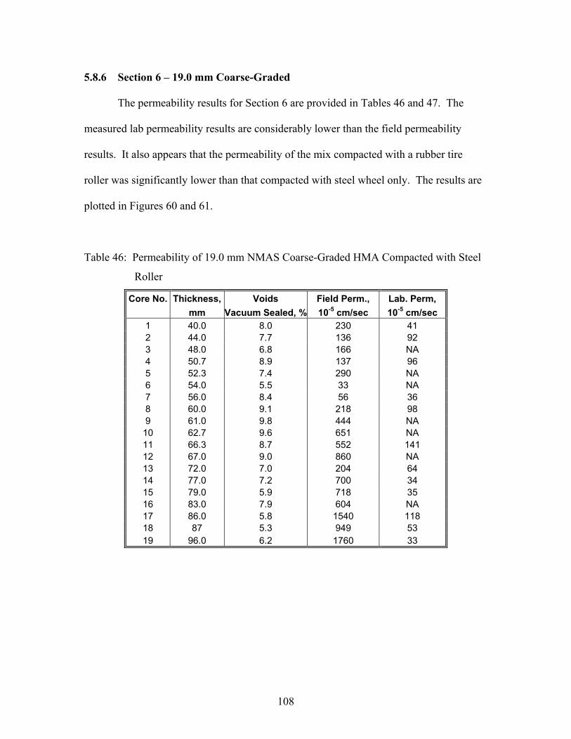
108

5.8.6 Section 6 – 19.0 mm Coarse-Graded

The permeability results for Section 6 are provided in Tables 46 and 47. The

measured lab permeability results are considerably lower than the field permeability

results. It also appears that the permeability of the mix compacted with a rubber tire

roller was significantly lower than that compacted with steel wheel only. The results are

plotted in Figures 60 and 61.

Table 46: Permeability of 19.0 mm NMAS Coarse-Graded HMA Compacted with Steel

Roller

Core No. Thickness, Voids Field Perm., Lab. Perm, mm Vacuum Sealed, % 10-5 cm/sec 10-5 cm/sec 1 40.0 8.0 230 41 2 44.0 7.7 136 92 3 48.0 6.8 166 NA 4 50.7 8.9 137 96 5 52.3 7.4 290 NA 6 54.0 5.5 33 NA 7 56.0 8.4 56 36 8 60.0 9.1 218 98 9 61.0 9.8 444 NA

10 62.7 9.6 651 NA 11 66.3 8.7 552 141 12 67.0 9.0 860 NA 13 72.0 7.0 204 64 14 77.0 7.2 700 34 15 79.0 5.9 718 35 16 83.0 7.9 604 NA 17 86.0 5.8 1540 118 18 87 5.3 949 53 19 96.0 6.2 1760 33

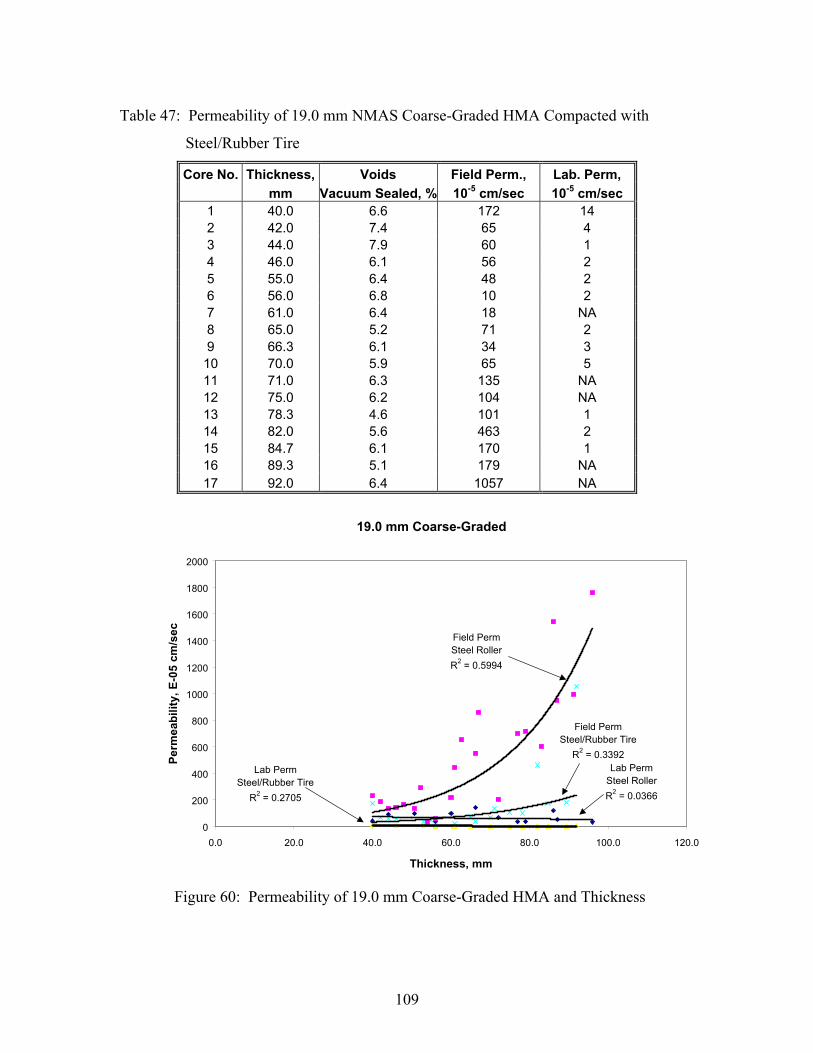
109

Table 47: Permeability of 19.0 mm NMAS Coarse-Graded HMA Compacted with

Steel/Rubber Tire

Core No. Thickness, Voids Field Perm., Lab. Perm, mm Vacuum Sealed, % 10-5 cm/sec 10-5 cm/sec 1 40.0 6.6 172 14 2 42.0 7.4 65 4 3 44.0 7.9 60 1 4 46.0 6.1 56 2 5 55.0 6.4 48 2 6 56.0 6.8 10 2 7 61.0 6.4 18 NA 8 65.0 5.2 71 2 9 66.3 6.1 34 3

10 70.0 5.9 65 5 11 71.0 6.3 135 NA 12 75.0 6.2 104 NA 13 78.3 4.6 101 1 14 82.0 5.6 463 2 15 84.7 6.1 170 1 16 89.3 5.1 179 NA 17 92.0 6.4 1057 NA





R2 = 0.3392Lab Perm

Steel/Rubber TireR2 = 0.2705

0

200

400

600

800

1000

1200

1400

1600

1800

2000

0.0 20.0 40.0 60.0 80.0 100.0 120.0

Thickness, mm

Perm

eabi

lity,

E-0

5 cm

/sec

Figure 60: Permeability of 19.0 mm Coarse-Graded HMA and Thickness

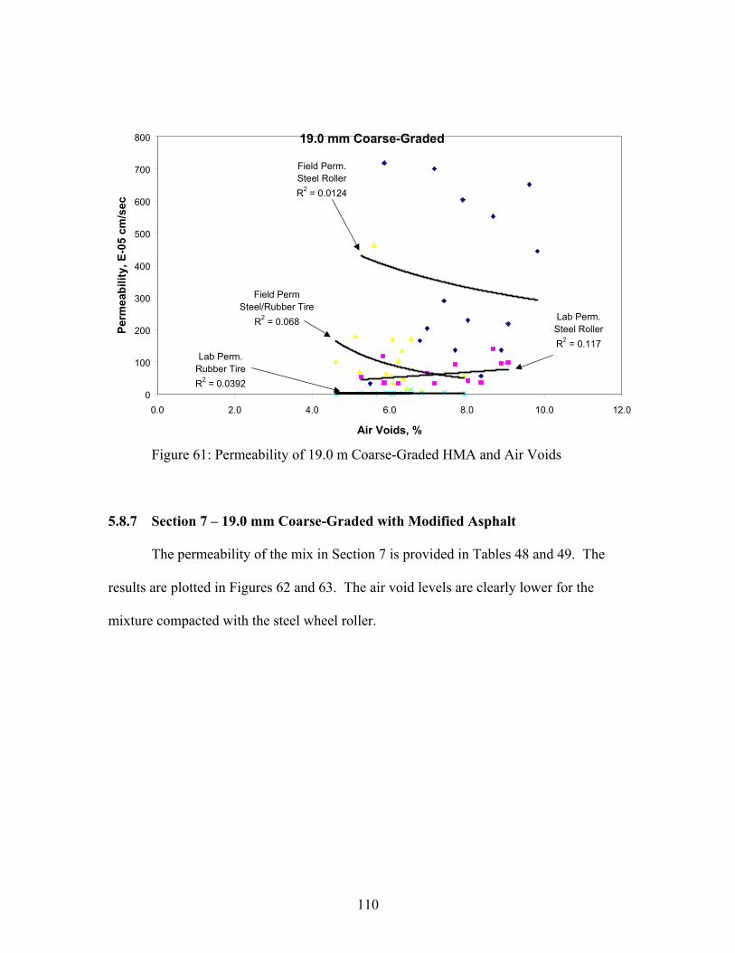
110

Figure 61: Permeability of 19.0 m Coarse-Graded HMA and Air Voids

5.8.7 Section 7 – 19.0 mm Coarse-Graded with Modified Asphalt

The permeability of the mix in Section 7 is provided in Tables 48 and 49. The

results are plotted in Figures 62 and 63. The air void levels are clearly lower for the

mixture compacted with the steel wheel roller.



Field Perm Steel/Rubber Tire

R2 = 0.068


Lab Perm.Rubber TireR2 = 0.0392

0

100

200

300

400

500

600

700

800

0.0 2.0 4.0 6.0 8.0 10.0 12.0

Air Voids, %

Perm

eabi

lity,

E-0

5 cm

/sec

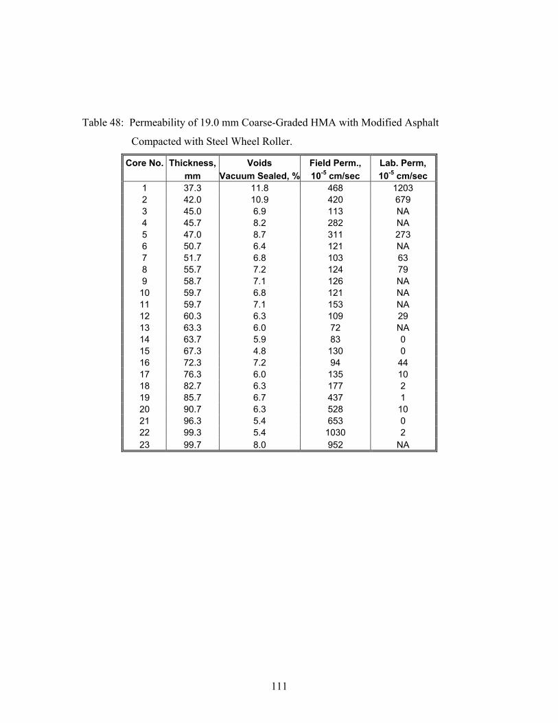
111

Table 48: Permeability of 19.0 mm Coarse-Graded HMA with Modified Asphalt

Compacted with Steel Wheel Roller.

Core No. Thickness, Voids Field Perm., Lab. Perm, mm Vacuum Sealed, % 10-5 cm/sec 10-5 cm/sec 1 37.3 11.8 468 1203 2 42.0 10.9 420 679 3 45.0 6.9 113 NA 4 45.7 8.2 282 NA 5 47.0 8.7 311 273 6 50.7 6.4 121 NA 7 51.7 6.8 103 63 8 55.7 7.2 124 79 9 58.7 7.1 126 NA

10 59.7 6.8 121 NA 11 59.7 7.1 153 NA 12 60.3 6.3 109 29 13 63.3 6.0 72 NA 14 63.7 5.9 83 0 15 67.3 4.8 130 0 16 72.3 7.2 94 44 17 76.3 6.0 135 10 18 82.7 6.3 177 2 19 85.7 6.7 437 1 20 90.7 6.3 528 10 21 96.3 5.4 653 0 22 99.3 5.4 1030 2 23 99.7 8.0 952 NA

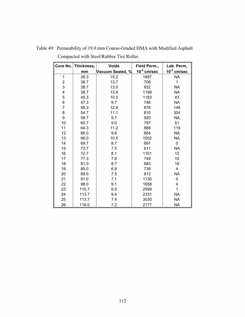
112

Table 49: Permeability of 19.0 mm Coarse-Graded HMA with Modified Asphalt

Compacted with Steel/Rubber Tire Roller.

Core No. Thickness, Voids Field Perm., Lab. Perm, mm Vacuum Sealed, % 10-5 cm/sec 10-5 cm/sec 1 36.3 15.2 1897 NA 2 38.7 13.7 706 1 3 38.7 13.0 832 NA 4 38.7 13.9 1199 NA 5 45.3 10.3 1183 43 6 47.3 9.7 746 NA 7 48.3 12.9 876 146 8 54.7 11.1 810 304 9 58.7 9.7 920 NA

10 60.7 9.0 797 51 11 64.3 11.2 888 119 12 66.0 9.6 664 NA 13 66.0 10.5 1002 NA 14 69.7 8.7 897 0 15 72.7 7.5 611 NA 16 72.7 8.1 1101 12 17 77.3 7.6 749 10 18 81.0 8.7 683 18 19 85.0 6.9 738 4 20 89.0 7.5 812 NA 21 91.0 7.1 1130 0 22 98.0 9.1 1658 4 23 110.7 6.9 2599 1 24 113.7 9.4 2331 NA 25 113.7 7.4 3030 NA 26 116.0 7.2 2177 NA

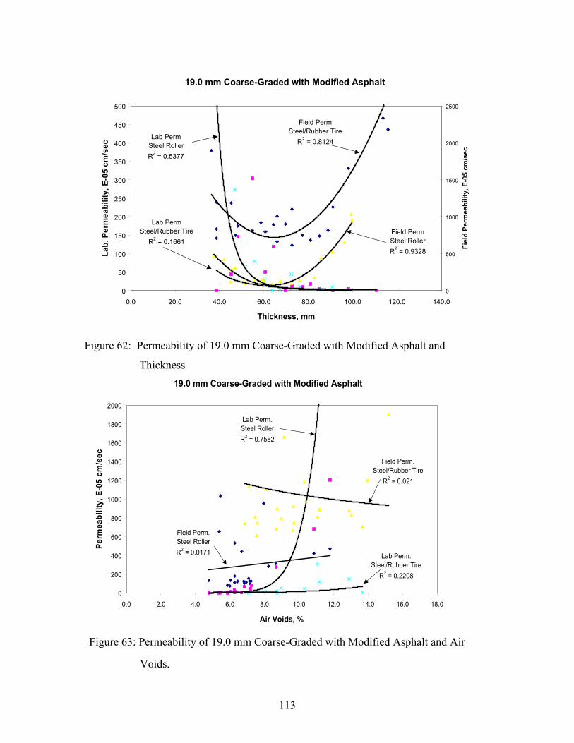
113

Figure 62: Permeability of 19.0 mm Coarse-Graded with Modified Asphalt and

Thickness



R2 = 0.1661



R2 = 0.8124


0

50

100

150

200

250

300

350

400

450

500

0.0 20.0 40.0 60.0 80.0 100.0 120.0 140.0

Thickness, mm

Lab.

Per

mea

bilit

y, E

-05

cm/s

ec

0

500

1000

1500

2000

2500

Fiel

d Pe

rmea

bilit

y, E

-05

cm/s

ec


Field Perm.Steel/Rubber Tire

R2 = 0.021


Field Perm.Steel RollerR2 = 0.0171 Lab Perm.

Steel/Rubber TireR2 = 0.2208

0

200

400

600

800

1000

1200

1400

1600

1800

2000

0.0 2.0 4.0 6.0 8.0 10.0 12.0 14.0 16.0 18.0

Air Voids, %

Perm

eabi

lity,

E-0

5 cm

/se c

Figure 63: Permeability of 19.0 mm Coarse-Graded with Modified Asphalt and Air

Voids.

114

5.9 Part 2– Evaluation of Relationship of Laboratory Permeability, Density and

Lift Thickness of Field Compacted Cores

Table 50 provides the average thickness of the cores obtained from NCHRP 9-

9(1) projects, the average air void content by the SSD method, the average air void

content by the vacuum sealed method, the average water absorption from SSD testing,

and the average laboratory permeability values. Based on the discussion in the first part

of this research that compared the SSD method and the vacuum sealed method, it was

decided to use the air voids determined from vacuum sealed method in the analysis.

Figure 64 illustrates the relationship between in-place air voids and permeability

for all cores. The R2 value for this figure is relatively high (0.66) and the relationship is

significant (p-value = 0.000). In this figure, the y-axis was reduced to show a clearer

relationship. Of the 287 data points, 18 data points having permeability values larger

than 1000 x 10-5 cm/sec are not shown in the figure. The largest permeability value was

12,800 x 10-5 cm/s. The data shows that as the in-place air voids increased, permeability

also increased. Based on the trend line, permeability is very low at air void content less

than 6 to 8 percent. The permeability starts to increase at a greater rate with changes in

in-place air voids above 8 percent.

The relationship between in-place air voids and permeability for the 9.5 mm

NMAS mix is illustrated in Figure 65. The R2 values for both coarse-graded and fine-

graded mixes were relatively high (0.70 and 0.86, respectively) and both relationships are

significant (p-value = 0.000). For both gradation types, the permeability begins to

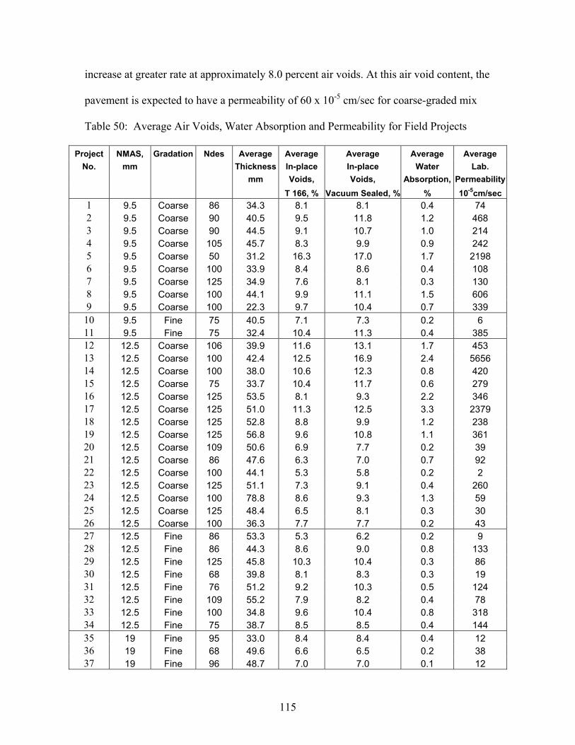
115

increase at greater rate at approximately 8.0 percent air voids. At this air void content, the

pavement is expected to have a permeability of 60 x 10-5 cm/sec for coarse-graded mix

Table 50: Average Air Voids, Water Absorption and Permeability for Field Projects

Project NMAS, Gradation Ndes Average Average Average Average Average No. mm Thickness In-place In-place Water Lab.

mm Voids, Voids, Absorption, Permeability T 166, % Vacuum Sealed, % % 10-5cm/sec 1 9.5 Coarse 86 34.3 8.1 8.1 0.4 74 2 9.5 Coarse 90 40.5 9.5 11.8 1.2 468 3 9.5 Coarse 90 44.5 9.1 10.7 1.0 214 4 9.5 Coarse 105 45.7 8.3 9.9 0.9 242 5 9.5 Coarse 50 31.2 16.3 17.0 1.7 2198 6 9.5 Coarse 100 33.9 8.4 8.6 0.4 108 7 9.5 Coarse 125 34.9 7.6 8.1 0.3 130 8 9.5 Coarse 100 44.1 9.9 11.1 1.5 606 9 9.5 Coarse 100 22.3 9.7 10.4 0.7 339

10 9.5 Fine 75 40.5 7.1 7.3 0.2 6 11 9.5 Fine 75 32.4 10.4 11.3 0.4 385 12 12.5 Coarse 106 39.9 11.6 13.1 1.7 453 13 12.5 Coarse 100 42.4 12.5 16.9 2.4 5656 14 12.5 Coarse 100 38.0 10.6 12.3 0.8 420 15 12.5 Coarse 75 33.7 10.4 11.7 0.6 279 16 12.5 Coarse 125 53.5 8.1 9.3 2.2 346 17 12.5 Coarse 125 51.0 11.3 12.5 3.3 2379 18 12.5 Coarse 125 52.8 8.8 9.9 1.2 238 19 12.5 Coarse 125 56.8 9.6 10.8 1.1 361 20 12.5 Coarse 109 50.6 6.9 7.7 0.2 39 21 12.5 Coarse 86 47.6 6.3 7.0 0.7 92 22 12.5 Coarse 100 44.1 5.3 5.8 0.2 2 23 12.5 Coarse 125 51.1 7.3 9.1 0.4 260 24 12.5 Coarse 100 78.8 8.6 9.3 1.3 59 25 12.5 Coarse 125 48.4 6.5 8.1 0.3 30 26 12.5 Coarse 100 36.3 7.7 7.7 0.2 43 27 12.5 Fine 86 53.3 5.3 6.2 0.2 9 28 12.5 Fine 86 44.3 8.6 9.0 0.8 133 29 12.5 Fine 125 45.8 10.3 10.4 0.3 86 30 12.5 Fine 68 39.8 8.1 8.3 0.3 19 31 12.5 Fine 76 51.2 9.2 10.3 0.5 124 32 12.5 Fine 109 55.2 7.9 8.2 0.4 78 33 12.5 Fine 100 34.8 9.6 10.4 0.8 318 34 12.5 Fine 75 38.7 8.5 8.5 0.4 144 35 19 Fine 95 33.0 8.4 8.4 0.4 12 36 19 Fine 68 49.6 6.6 6.5 0.2 38 37 19 Fine 96 48.7 7.0 7.0 0.1 12

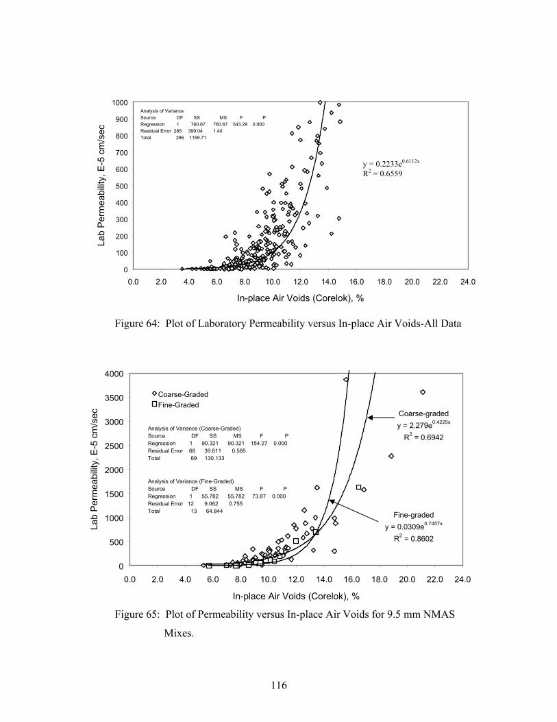
116

0

100

200

300

400

500

600

700

800

900

1000

0.0 2.0 4.0 6.0 8.0 10.0 12.0 14.0 16.0 18.0 20.0 22.0 24.0

In-place Air Voids (Corelok), %

Lab

Per

mea

bilit

y, E

-5 c

m/s

ecAnalysis of VarianceSource DF SS MS F PRegression 1 760.67 760.67 543.29 0.000Residual Error 285 399.04 1.40Total 286 1159.71

Figure 64: Plot of Laboratory Permeability versus In-place Air Voids-All Data

Coarse-gradedy = 2.279e0.4225x

R2 = 0.6942

Fine-gradedy = 0.0309e0.7457x

R2 = 0.8602

0

500

1000

1500

2000

2500

3000

3500

4000

0.0 2.0 4.0 6.0 8.0 10.0 12.0 14.0 16.0 18.0 20.0 22.0 24.0


Lab

Per

mea

bilit

y, E

-5 c

m/s

ec

Coarse-GradedFine-Graded

Analysis of Variance (Coarse-Graded)Source DF SS MS F PRegression 1 90.321 90.321 154.27 0.000Residual Error 68 39.811 0.585Total 69 130.133

Analysis of Variance (Fine-Graded)Source DF SS MS F PRegression 1 55.782 55.782 73.87 0.000Residual Error 12 9.062 0.755Total 13 64.844

Figure 65: Plot of Permeability versus In-place Air Voids for 9.5 mm NMAS

Mixes.

y = 0.2233e0.6112x R2 = 0.6559

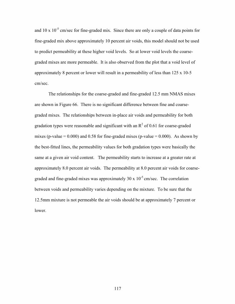
117

and 10 x 10-5 cm/sec for fine-graded mix. Since there are only a couple of data points for

fine-graded mix above approximately 10 percent air voids, this model should not be used

to predict permeability at these higher void levels. So at lower void levels the coarse-

graded mixes are more permeable. It is also observed from the plot that a void level of

approximately 8 percent or lower will result in a permeability of less than 125 x 10-5

cm/sec.

The relationships for the coarse-graded and fine-graded 12.5 mm NMAS mixes

are shown in Figure 66. There is no significant difference between fine and coarse-

graded mixes. The relationships between in-place air voids and permeability for both

gradation types were reasonable and significant with an R2 of 0.61 for coarse-graded

mixes (p-value = 0.000) and 0.58 for fine-graded mixes (p-value = 0.000). As shown by

the best-fitted lines, the permeability values for both gradation types were basically the

same at a given air void content. The permeability starts to increase at a greater rate at

approximately 8.0 percent air voids. The permeability at 8.0 percent air voids for coarse-

graded and fine-graded mixes was approximately 30 x 10-5 cm/sec. The correlation

between voids and permeability varies depending on the mixture. To be sure that the

12.5mm mixture is not permeable the air voids should be at approximately 7 percent or

lower.

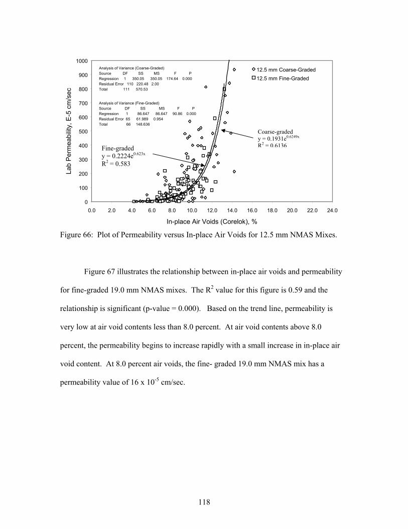
118

0

100

200

300

400

500

600

700

800

900

1000

0.0 2.0 4.0 6.0 8.0 10.0 12.0 14.0 16.0 18.0 20.0 22.0 24.0


Lab

Per

mea

bilit

y, E

-5 c

m/s

ec12.5 mm Coarse-Graded12.5 mm Fine-Graded

Analysis of Variance (Coarse-Graded)Source DF SS MS F PRegression 1 350.05 350.05 174.64 0.000Residual Error 110 220.48 2.00Total 111 570.53

Analysis of Variance (Fine-Graded)Source DF SS MS F PRegression 1 86.647 86.647 90.86 0.000Residual Error 65 61.989 0.954Total 66 148.636

Figure 66: Plot of Permeability versus In-place Air Voids for 12.5 mm NMAS Mixes.

Figure 67 illustrates the relationship between in-place air voids and permeability

for fine-graded 19.0 mm NMAS mixes. The R2 value for this figure is 0.59 and the

relationship is significant (p-value = 0.000). Based on the trend line, permeability is

very low at air void contents less than 8.0 percent. At air void contents above 8.0

percent, the permeability begins to increase rapidly with a small increase in in-place air

void content. At 8.0 percent air voids, the fine- graded 19.0 mm NMAS mix has a

permeability value of 16 x 10-5 cm/sec.

Coarse-graded y = 0.1931e0.6249x R2 = 0.6136Fine-graded

y = 0.2224e0.623x R2 = 0.583

119

y = 0.0437e0.7362x

R2 = 0.5923

0

20

40

60

80

100

120

140

0.0 2.0 4.0 6.0 8.0 10.0 12.0


Lab

Per

mea

bilit

y, E

-5 c

m/s

ecAnalysis of VarianceSource DF SS MS F PRegression 1 29.760 29.760 31.96 0.000Residual Error 22 20.483 0.931Total 23 50.243

Figure 67: Plot of Permeability versus In-place Air Voids for 19.0 mm Fine-

Graded NMAS mix.

In order to evaluate the factors affecting permeability, a multiple linear regression

(MLR) was performed. This procedure was conducted to identify factors most affecting

permeability. A best subsets regression was utilized to evaluate all independent variables

and select the variables that provided the most significant relationship with the dependent

variable (permeability). The best subsets regression procedure allows the user to input

numerous factors that have the potential to impact the dependent parameter. For this

analysis, the natural log of permeability was selected as the response, while natural log of

in-place air voids based on vacuum sealed method, NMAS, sample thickness, natural log

of voids in mineral aggregates (VMA), and coarse aggregate ratio were included as the

predictors. The coarse aggregate ratio was defined as the percent retained on a sieve,

three sizes lower than the NMAS divided by the percent passing that particular sieve.

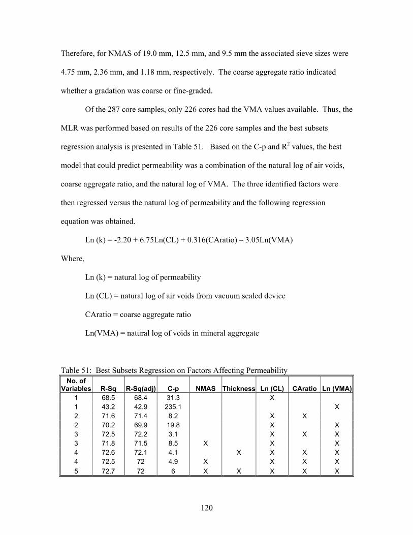
120

Therefore, for NMAS of 19.0 mm, 12.5 mm, and 9.5 mm the associated sieve sizes were

4.75 mm, 2.36 mm, and 1.18 mm, respectively. The coarse aggregate ratio indicated

whether a gradation was coarse or fine-graded.

Of the 287 core samples, only 226 cores had the VMA values available. Thus, the

MLR was performed based on results of the 226 core samples and the best subsets

regression analysis is presented in Table 51. Based on the C-p and R2 values, the best

model that could predict permeability was a combination of the natural log of air voids,

coarse aggregate ratio, and the natural log of VMA. The three identified factors were

then regressed versus the natural log of permeability and the following regression

equation was obtained.

Ln (k) = -2.20 + 6.75Ln(CL) + 0.316(CAratio) – 3.05Ln(VMA)

Where,

Ln (k) = natural log of permeability

Ln (CL) = natural log of air voids from vacuum sealed device

CAratio = coarse aggregate ratio

Ln(VMA) = natural log of voids in mineral aggregate

Table 51: Best Subsets Regression on Factors Affecting Permeability No. of

Variables R-Sq R-Sq(adj) C-p NMAS Thickness Ln (CL) CAratio Ln (VMA)1 68.5 68.4 31.3 X 1 43.2 42.9 235.1 X 2 71.6 71.4 8.2 X X 2 70.2 69.9 19.8 X X 3 72.5 72.2 3.1 X X X 3 71.8 71.5 8.5 X X X 4 72.6 72.1 4.1 X X X X 4 72.5 72 4.9 X X X X 5 72.7 72 6 X X X X X

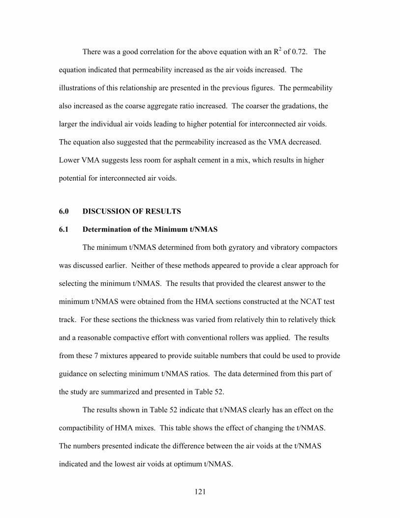
121

There was a good correlation for the above equation with an R2 of 0.72. The

equation indicated that permeability increased as the air voids increased. The

illustrations of this relationship are presented in the previous figures. The permeability

also increased as the coarse aggregate ratio increased. The coarser the gradations, the

larger the individual air voids leading to higher potential for interconnected air voids.

The equation also suggested that the permeability increased as the VMA decreased.

Lower VMA suggests less room for asphalt cement in a mix, which results in higher

potential for interconnected air voids.

6.0 DISCUSSION OF RESULTS

6.1 Determination of the Minimum t/NMAS

The minimum t/NMAS determined from both gyratory and vibratory compactors

was discussed earlier. Neither of these methods appeared to provide a clear approach for

selecting the minimum t/NMAS. The results that provided the clearest answer to the

minimum t/NMAS were obtained from the HMA sections constructed at the NCAT test

track. For these sections the thickness was varied from relatively thin to relatively thick

and a reasonable compactive effort with conventional rollers was applied. The results

from these 7 mixtures appeared to provide suitable numbers that could be used to provide

guidance on selecting minimum t/NMAS ratios. The data determined from this part of

the study are summarized and presented in Table 52.

The results shown in Table 52 indicate that t/NMAS clearly has an effect on the

compactibility of HMA mixes. This table shows the effect of changing the t/NMAS.

The numbers presented indicate the difference between the air voids at the t/NMAS

indicated and the lowest air voids at optimum t/NMAS.

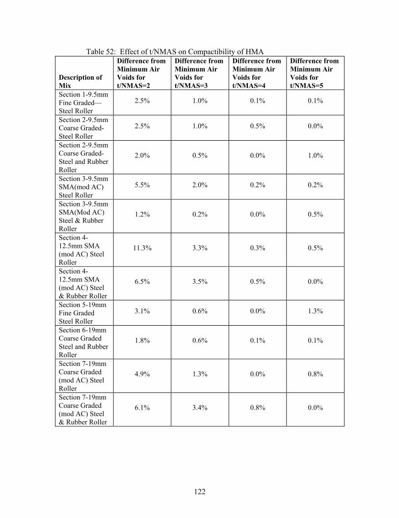
122

Table 52: Effect of t/NMAS on Compactibility of HMA

Description of Mix

Difference from Minimum Air Voids for t/NMAS=2




Section 1-9.5mm Fine Graded—Steel Roller

2.5% 1.0% 0.1% 0.1%

Section 2-9.5mm Coarse Graded-Steel Roller

2.5% 1.0% 0.5% 0.0%

Section 2-9.5mm Coarse Graded-Steel and Rubber Roller

2.0% 0.5% 0.0% 1.0%

Section 3-9.5mm SMA(mod AC) Steel Roller

5.5% 2.0% 0.2% 0.2%

Section 3-9.5mm SMA(Mod AC) Steel & Rubber Roller

1.2% 0.2% 0.0% 0.5%

Section 4-12.5mm SMA (mod AC) Steel Roller

11.3% 3.3% 0.3% 0.5%

Section 4-12.5mm SMA (mod AC) Steel & Rubber Roller

6.5% 3.5% 0.5% 0.0%

Section 5-19mm Fine Graded Steel Roller

3.1% 0.6% 0.0% 1.3%

Section 6-19mm Coarse Graded Steel and Rubber Roller

1.8% 0.6% 0.1% 0.1%

Section 7-19mm Coarse Graded (mod AC) Steel Roller

4.9% 1.3% 0.0% 0.8%

Section 7-19mm Coarse Graded (mod AC) Steel & Rubber Roller

6.1% 3.4% 0.8% 0.0%

123

A t/NMAS of 4 seems to be about optimum however a closer look is needed since

there are a number of different mix types. The data suggest that there is a greater than 2

percent difference in air voids between the results at a ratio of 3 and the ratio that gives

the lowest air voids. This signifies that for a given compactive effort the air voids at a

t/NMAS ratio of 3 will generally be about 2% higher than the optimum t/NMAS.

However, this finding is for a constant compactive effort. Increasing the compactive

effort will allow an adequate density to be obtained in many cases even when the

t/NMAS is not optimum.

In all cases a t/NMAS of 2 provided air voids more than 1% greater than the air

voids obtained at optimum t/NMAS. In most cases the difference in density between

t/NMAS of 2 and optimum exceeded 2.5%. This indicates that one would expect to see

approximately 2.5% higher air voids when the t/NMAS was 2 than when it was close to

optimum.

For fine-graded mixes it appears that the desired minimum t/NMAS is 3. There

were only 2 fine-graded mixes evaluated and both were within 1 percent of the optimum

voids at a t/NMAS equal to 3. There were 3 coarse-graded mixes evaluated and 2 of the

3 mixes had air voids within 1 percent of optimum at a t/NMAS equal to 3. The SMA

mixes appeared to deviate even more from optimum at a t/NMAS of 3. However, a

t/NMAS looks satisfactory for SMA mixtures. The results are all very consistent: a

t/NMAS of 4 nearly always appeared to be about optimum. In three cases a t/NMAS of 5

was closer to the lowest air voids but the air voids difference at t/NMAS of 4 was still

very low. In summary the data indicates that a minimum thickness t/NMAS of 4 is

preferred for coarse-graded mixes and SMA mixes. For fine-graded mixes this minimum

124

t/NMAS can be reduced to 3 without adversely affecting the compactibility of the

mixtures.

6.2 Effect of Mix Temperature on Compaction

When looking at the effect of t/NMAS on density one must also look at the effect

of mat thickness and cooling rate. One of the reasons that lower t/NMAS ratios are

difficult to compact is the effect of cooling. A thin section regardless of the t/NMAS will

cool quickly and therefore be difficult to compact. When large NMAS aggregate is used

the rate of cooling is relatively low even when the t/NMAS is low. There was some

indication that the t/NMAS could be smaller for larger NMAS and the cooling rate is

likely the reason. A 19mm mix placed at a t/NMAS of 2 is still 38mm thick which will

hold the heat for a reasonable period of time. However, a 9.5mm mix placed at a

t/NMAS of 2 is only 19mm thick and will cool very quickly.

The temperature data collected from the test sections showed that for the

conditions during the tests a 25mm layer thickness cooled at about twice the rate as a

37.5mm layer thickness. Hence it would require twice as many rollers to roll the 25mm

layer the same number of passes at the same speed over the same temperature range. So

care must be used when selecting the layer thickness to ensure adequate rolling time. A

25mm layer thickness is very difficult to compact prior to cooling especially when paving

in cold weather. To ensure adequate compaction the layer thickness should be closer to

37.5mm thick.

125

6.3 Effect of thickness on permeability at 7.0 ± 1.0 percent air voids

It is difficult to compact mixes to a reasonable density for thin lifts using the

gyratory compactor. The problem is more pronounced when compacting SMA mixes.

However, specimens compacted with vibratory compactor did achieve the target air voids

at t/NMAS of 2.0, 3.0 and 4.0. The results in general show the permeability decreases as

t/NMAS increases. Of all the mixes tested, only the 9.5 mm and 12.5 mm NMAS SMA

mixes compacted at t/NMAS of 2.0 had permeability values more than 125 x 10-5 cm/sec.

Results from Tables 36 and 37 are interesting in that specimens that had similar air void

content, gradation and thickness had different permeability values. In most cases,

specimens compacted with the vibratory compactor had much lower permeability than

specimens compacted with gyratory compactor. This could likely be explained by a

study conducted by Cooley and Kandhal (14) comparing compaction performed by

vibratory and gyratory compactor. Specimens compacted by vibratory had more

compaction at the top whereas gyratory-compacted samples showed less compaction in

the top and bottom and more in the middle. This low compaction around the top, bottom,

and outside edge for gyratory samples can significantly increase the permeability.

6.4 Evaluation of Factors Affecting Permeability

Observation of Figures 65 and 66 suggests that there is no significant difference

between fine and coarse-graded mixes based on laboratory permeability tests. Cooley et

al. (15) suggested a critical in-place air void content of 7.7 percent for both 9.5 and 12.5

mm NMAS coarse-graded mixes (based on field permeability value of 100 x 10-5

cm/sec). Using the critical value, the 9.5 mm coarse-graded mix has a lab permeability

126

value of 60 x 10-5 cm/sec and the 12.5 mm coarse graded mix has a lab permeability

value of 24 x 10-5cm/sec. The field permeability test is really an index and not a true

measure of permeability so there is no surprise that there is a difference between field and

lab results.

The selected factors identified by the multiple linear regression are interesting in

that NMAS was not among the factors identified as affecting permeability. However,

this can likely be explained in that of the 37 projects included in this study, 34 had either

a 9.5 or 12.5 mm NMAS. Therefore, there was a little variation in NMAS, which would

cause it not to be identified during the regression.

7.0 CONCLUSIONS

Based upon the results of this study, the following conclusions can be drawn.

The density that can be obtained under normal rolling conditions is clearly related

to the t/NMAS. For improved compactibility it is recommended that the t/NMAS be at

least 3 for fine graded mixes and at least 4 for coarse graded mixes. The data for SMA

indicates that the ratio should also be at least 4. Ratios less than these suggested numbers

could be used but it would generally require more compactive effort to obtain the desired

density. In most cases a t/NMAS of 5 does not result in the need for more compactive

effort to obtain maximum density. However, care must be exercised when the thickness

gets too large to ensure that adequate density is obtained.

The results of the evaluation of the effect of mix temperature on the relationship

between density and t/NMAS indicate that one of the reasons for low density at thinner

sections (lower t/NMAS) is the more rapid cooling of the mixture. Hence, for thinner

127

layers it is even more important that rollers stay very close to the paver so that rolling can

be accomplished prior to excessive cooling. For the conditions of this study the mixes

placed at 25mm thickness cooled twice as fast as mixes placed at 37.5mm thickness. For

thicker sections (larger t/NMAS) rate of cooling is typically not a problem.

The in-place void content is the most significant factor impacting permeability of

Superpave pavements. This is followed by coarse aggregate ratio and VMA. As the

values of coarse aggregate ratio increases, permeability increases. Permeability decreases

as VMA increases.

The variability of permeability between various mixtures is very high. Some

mixtures are permeable at the 8 to 10 percent void range and others do not seem to be

permeable at these higher voids. However, to ensure that permeability is not a problem

the in-place air voids should be between 6 and 7 percent or lower. This appears to be true

for a wide range of mixtures regardless of NMAS and grading.

8.0 REFERENCES

1. Roberts, F.L., P.S. Kandhal, E.R. Brown, D.Y. Lee, and T.W, Kennedy. Hot Mix

Asphalt Materials, Mixture Design, and Construction. NAPA Education

Foundation, Lanham, MD. Second Ed., 1996.

2. Zube, E. “Compaction Studies of Asphalt Concrete Pavements as Related to the

Water Permeability Test.” Highway Research Board, Bulletin 358, 1962.

3. Brown, E.R., R. Collins, and J.A. Brownfield. “Investigation of Segregation of

Asphalt Mixtures in the State of Georgia.” Transportation Research Record 1217,

1989.

128

4. Choubane, B., G.C. Page, and J.A. Musselman. “Investigation of Water

Permeability of Coarse Graded Superpave Pavements.” Journal of the Association

of Asphalt Paving Technologists, Volume 67, 1998.

5. Ford, M.C., and C.E. McWilliams. “Asphalt Mix Permeability.” University of

Arkansas, Fayettville, AR, 1988.

6. Hudson, S.B., and R.L. Davis. “Relationship of Aggregate Voidage to Gradation.”

Association of Asphalt Paving Technologists, Volume 34, 1965.

7. Mallick, R.B., L.A. Cooley, Jr., and M. Teto. “Evaluation of Permeability of

Superpave Mixes in Maine, Final Report. Technical Report ME-001, November

1999.

8. Musselman, J.A., B. Choubane, G.C. Page, and P.B. Upshaw. “Superpave Field

Implementation: Florida’s Early Experience.” Transportation Research Record

1609, 1998.

9. Westerman, J.R. AHTD’s Experience with Superpave Pavement Permeability.

Presented at Arkansas Superpave Symposium, January 21, 1998.

10. ‘Superpave Construction Guidelines.’ National Asphalt Pavement Association.

Special Report 180. Lanham, Maryland. October 1997.

11. Garcia, J., K. Hansen. “HMA Pavement Mix Type Selection Guide.” National

Asphalt Pavement Association. Information Series 128, 2001.

12. Cooley, Jr., L.A., B.D. Prowell, M.R. Hainin, M.S. Buchanan, and J. Harrington.

Bulk Specific Gravity Round Robin Using the Corelok Vacuum Sealing Device.

National Center for Asphalt Technology (NCAT) Report No. 02-11. November

2002.

129

13. The Asphalt Handbook. Asphalt Institute Manual Series No. 4 (MS-4) 1989.

14. Cooley, Jr., and P.S. Kandhal, “Evaluation of Density Gradients in Loaded Wheel

Tester Samples,” Journal of Testing and Evaluation, Volume 28, No. 6,

November 2000.

15. L.A.Cooley, Jr.E.R. Brown, and S. Maghsoodloo. “Development of Critical Field

Permeability and Pavement Density Values for Coarse-Graded Superpave

Pavements.” Prepared for Presentation and Publication at the 80th Annual

Meeting of the Transportation Research Board. January 2001.

Documents

Relationships of HMA In-Place Air Voids, Lift Thickness ...onlinepubs.trb.org/onlinepubs/nchrp/nchrp_w68v1.pdf · Voids, Lift Thickness, and Permeability Prepared for: National Cooperative