Relative importance of second-order terms in relativistic dissipative fluid dynamics

Relative importance of second-order terms in relativisticdissipative fluid dynamics

E. Molnár,1,2 H. Niemi,3,4 G. S. Denicol,5 and D. H. Rischke61MTA-DE Particle Physics Research Group, P.O. Box 105, H-4010 Debrecen, Hungary

2Frankfurt Institute for Advanced Studies, Ruth-Moufang-Strasse 1,D-60438 Frankfurt am Main, Germany

3Department of Physics, University of Jyväskylä, P.O. Box 35 (YFL), FI-40014 Jyväskylä, Finland4Helsinki Institute of Physics, University of Helsinki, P.O. Box 64, FI-00014 Helsinki, Finland

5Department of Physics, McGill University, 3600 University Street, Montréal, Quebec H3A 2T8, Canada6Institut für Theoretische Physik, Johann Wolfgang Goethe-Universität, Max-von-Laue-Strasse 1,

D-60438 Frankfurt am Main, Germany(Received 4 August 2013; published 3 April 2014)

In Denicol et al. [Phys. Rev. D 85, 114047 (2012)], the equations of motion of relativistic dissipativefluid dynamics were derived from the relativistic Boltzmann equation. These equations contain a multitudeof terms of second order in the Knudsen number, in the inverse Reynolds number, or their product. Terms ofsecond order in the Knudsen number give rise to nonhyperbolic (and thus acausal) behavior and must beneglected in (numerical) solutions of relativistic dissipative fluid dynamics. The coefficients of the termswhich are of the order of the product of Knudsen and inverse Reynolds numbers have been explicitlycomputed in the above reference, in the limit of a massless Boltzmann gas. Terms of second order in theinverse Reynolds number arise from the collision term in the Boltzmann equation, upon expansion tosecond order in deviations from the single-particle distribution function in local thermodynamicalequilibrium. In this work, we compute these second-order terms for a massless Boltzmann gas withconstant scattering cross section. Consequently, we assess their relative importance in comparison to theterms which are of the order of the product of the Knudsen and inverse Reynolds numbers.DOI: 10.1103/PhysRevD.89.074010 PACS numbers: 51.10.+y, 12.38.Mh, 24.10.Nz, 47.75.+f

I. INTRODUCTION AND CONCLUSIONS

Relativistic fluid dynamics has found widespread appli-cations in heavy-ion physics, in modeling nuclear colli-sions at ultrarelativistic bombarding energies [1,2], inastrophysics, for instance in modeling binary mergers ofcompact stellar objects (see e.g. Ref. [3]), as well as incosmology [4–8]. In the past, in order to solve theequations of motion of relativistic fluid dynamics, onehas often made the assumption that the fluid is ideal, i.e.,one demands instantaneous local thermodynamical equi-librium, which in turn allows to neglect all dissipativeeffects. However, there are no ideal fluids in nature, ascan be seen for instance from the fact that the shearviscosity coefficient may attain a lower limit, but nevervanishes [9–11].A more realistic modeling of the dynamics of relativistic

fluids thus demands that one uses the equations ofrelativistic dissipative fluid dynamics. The first attemptsto formulate such equations were made by Eckart [12] andLandau and Lifshitz [13] based on a relativistic generali-zation of the nonrelativistic Navier-Stokes equations.However, their equations suffer from instabilities andacausal signal propagation [14]. The reason for this isthe (erroneous) assumption that the dissipative quantities,like bulk viscous pressure Π, particle diffusion current nμ,and shear-stress tensor πμν, react instantaneously to the

thermodynamic forces, like gradients of the fluid velocityor temperature and chemical potential. If one relaxes thisassumption by introducing certain time scales τΠ, τn, andτπ , on which the dissipative quantities are allowed toapproach the values determined by the correspondingthermodynamic forces, these problems can be cured (pro-vided the relaxation times fulfill certain conditions [15]).Similar to earlier works by Grad [16] and Müller [17–19] inthe nonrelativistic context, Israel and Stewart (IS) wereamong the first to suggest equations of motion for relativ-istic dissipative fluids that were stable and causal [20–22].In recent years, relativistic dissipative fluid dynamics

based on the IS formulation was extensively applied todescribe the dynamics of nuclear collisions. At the sametime, the theoretical foundations of this theory were furtherexplored both from kinetic theory [23–40] and fromirreversible thermodynamics [41–51]. In particular, inRefs. [23–25] it has been investigated how to derive theequations of motion for the dissipative quantities using theBoltzmann equation as the underlying microscopic theory.In Ref. [24] a derivation of the equations of motion of

relativistic dissipative fluid dynamics was presented, whichis based on a systematic power-counting scheme in theKnudsen and inverse Reynolds number. The Knudsennumber, Kn ¼ λ=L, is the ratio between a characteristicmicroscopic time/length scale, λ (e.g., the mean-free pathbetween collisions), and a characteristic macroscopic scale

PHYSICAL REVIEW D 89, 074010 (2014)

1550-7998=2014=89(7)=074010(30) 074010-1 © 2014 American Physical Society

http://dx.doi.org/10.1103/PhysRevD.89.074010




of the fluid L. In this context, the inverse Reynoldsnumbers are the ratios of dissipative quantities and (local)equilibrium values of macroscopic fields, e.g. R−1

Π ¼jΠj=P0, R−1

n ¼ jnμj=n0, or R−1π ¼ jπμνj=P0, where P0 is

the thermodynamic pressure and n0 is the particle density inequilibrium. The time scales τΠ, τn, and τπ are identifiedwith the slowest microscopic time scales of the Boltzmannequation.The physical picture that emerges is that microscopic

processes (i.e., in the case of the Boltzmann equation,binary collisions) occur on time scales smaller than (or, atmost, as large as) τΠ, τn, and τπ . These processes affect thatthe dissipative quantitiesΠ, nμ, and πμν approach the valuesgiven by the (relativistic generalization of the) Navier-Stokes equations on the time scales τΠ, τn, and τπ . Sincemicroscopic physics influences the motion of the fluid onlyon short time scales, the term “transient fluid dynamics”was coined for such theories of relativistic dissipative fluiddynamics. The fact that the microscopic dynamics of theBoltzmann equation gives rise to relaxation-type equationsof motion for the dissipative quantities, i.e., where thesequantities exponentially decay towards the values given bythe Navier-Stokes equations, was confirmed in Ref. [52].It was also shown in that paper that approaches based onthe AdS/CFT correspondence lead to equations of motionwhich are of the type encountered for an underdamped

harmonic oscillator. The relaxation towards the Navier-Stokes values is then not exponential but oscillatory.Let us recall the relaxation-type equations for the

dissipative quantities derived in Ref. [24],

τΠ _Πþ Π ¼ −ζθ þ J þKþR; (1)

τn _nhμi þ nμ ¼ κIμ þ J μ þKμ þRμ; (2)

τπ _πhμνi þ πμν ¼ 2ησμν þ J μν þKμν þRμν; (3)

where the overdot denotes the proper time derivative,_A≡DA ¼ uμ∂μA. Here, ζ is the coefficient of the bulkviscosity, κ the coefficient of particle diffusion (which isrelated to that of heat conduction) and η the coefficient ofshear viscosity. Furthermore, with the fluid four-velocity uμ

(chosen in the Landau frame), where uμuμ ¼ 1, with Δμν ¼gμν − uμuν being the three-projector onto the subspaceorthogonal to uμ, and with ∇μ ¼ Δμν∂ν being the three-gradient, θ ¼ ∇μuμ is the expansion scalar, σμν ≡∇hμuνi ¼12ð∇μuν þ∇νuμÞ − 1

3θΔμν is the shear tensor, while Iμ ¼

∇μα0 is the gradient of α0 ¼ μ=T, the ratio of chemicalpotential μ and temperature T.In the above equations, the tensors J , J μ, and J μν

contain all terms of first order in the product of the Knudsenand inverse Reynolds number,

J ¼ −lΠn∇ · n − τΠnn · F − δΠΠΠθ − λΠnn · I þ λΠππμνσμν;

J μ ¼ −τnnνωνμ − δnnnμθ − lnΠ∇μΠþ lnπΔμν∇λπλν þ τnΠΠFμ − τnππ

μνFν − λnnnνσμν þ λnΠΠIμ − λnππμνIν;

J μν ¼ 2τππhμλ ω

νiλ − δπππμνθ − τπππ

λhμσνiλ þ λπΠΠσμν − τπnnhμFνi þ lπn∇hμnνi þ λπnnhμIνi; (4)

where ωμν ¼ 12ð∇μuν − ∇νuμÞ denotes the vorticity and we defined Fμ ¼ ∇μP0 as the gradient of the thermodynamic

pressure. The tensors K, Kμ, and Kμν contain all terms of second order in the Knudsen number,

K ¼ ~ζ1ωμνωμν þ ~ζ2σμνσ

μν þ ~ζ3θ2 þ ~ζ4I · I þ ~ζ5F · F þ ~ζ6I · F þ ~ζ7∇ · I þ ~ζ8∇ · F;

Kμ ¼ ~κ1σμνIν þ ~κ2σ

μνFν þ ~κ3Iμθ þ ~κ4Fμθ þ ~κ5ωμνIν þ ~κ6Δ

μλ∇νσ

λν þ ~κ7∇μθ;

Kμν ¼ ~η1ωhμλ ω

νiλ þ ~η2θσμν þ ~η3σ

λhμσνiλ þ ~η4σhμλ ω

νiλ þ ~η5IhμIνi þ ~η6FhμFνi

þ ~η7IhμFνi þ ~η8∇hμIνi þ ~η9∇hμFνi: (5)

Note that, in contrast to Ref. [24], we now write the termproportional to ~κ6 with a three-gradient operator ∇ν insteadof a partial derivative ∂ν. Finally, the tensors R, Rμ, andRμν contain all terms of second order in the inverseReynolds number,

R ¼ φ1Π2 þ φ2n · nþ φ3πμνπμν; (6)

Rμ ¼ φ4nνπμν þ φ5Πnμ; (7)

Rμν ¼ φ6Ππμν þ φ7πλhμπνiλ þ φ8nhμnνi: (8)

These second-order terms follow from computing thecollision integral beyond linear order in the dissipativequantities.Observing the plethora of transport coefficients occur-

ring in Eqs. (4)–(8), a natural question to ask is whetherall of them are of the same order of magnitude, or whethersome coefficients are larger and thus more important thanothers. The goal of this paper is to answer this question.The coefficients in Eqs. (4) were explicitly computed inRef. [24] for a massless Boltzmann gas with constantscattering cross section. We now supplement these results

MOLNÁR et al. PHYSICAL REVIEW D 89, 074010 (2014)

074010-2

by computing the coefficients in Eqs. (5)–(8). We restrictourselves to the 14-moment approximation. In this case, thecoefficients in Eqs. (5) vanish identically (cf. Appendix I), andwe only need to focus on the coefficients φ1;…;φ8 inEqs. (6)–(8). The derivation and calculation of these coef-ficients is quite demanding and is presented in detail in theremainder of this paper. For the rest of this introductorysection, we simply quote the results and draw our conclusions.

For massless particles, the bulk viscous pressure van-ishes identically, Π ¼ 0, and we do not have to solveEq. (1). Also, terms in Eqs. (4)–(8) proportional toΠ can beneglected, such that we do not need to compute thecorresponding coefficients. Moreover, as mentioned above,in the 14-moment approximation all coefficients in Eqs. (5)vanish. Dividing Eq. (2) by n0, and Eq. (3) by P0, these twoequations can be written in the following form,

τn_nhμi

n0þ nμ

n0¼ κ

n0∇μα0

þ ðτnωμν − λnnσμν − δnnθgμνÞ

nνn0

þ lnπ

β0

Δμν∇λπλν

P0

−�τnπP0

β0

∇νP0

P0

þ λnπβ0

∇να0 − φ4P0

nνn0

�πμν

P0

; (9)

τπ_πhμνi

P0

þ πμν

P0

¼ 2η

P0

σμν

þ πhμλP0

�2τπω

νiλ − τππσνiλ − δππθgνiλ þ φ7P0

πνiλ

P0

�

þ lπnβ0∇hμnνi

n0þ nhμ

n0

�λπnβ0∇νiα0 − τπnn0

∇νiP0

P0

þ φ8β20P0

nνi

n0

�: (10)

Here, we have made use of the equation of state of themassless Boltzmann gas, P0 ¼ n0=β0, with β0 ¼ 1=T. Bydividing the dissipative quantities by n0 or P0, respec-tively, we immediately identify terms which are propor-tional to the inverse Reynolds number. Furthermore, thecoefficients of terms involving gradients (or time deriv-atives) all have dimension of time (or mean-free path)and are thus proportional to the Knudsen number. In thisform, it is easy to apply power-counting arguments toestimate the order of magnitude of the various terms. TheNavier-Stokes terms appearing in the first lines are of firstorder in the Knudsen number. The second lines containterms proportional to the dissipative quantity that is evolvedin the respective equation (nμ in the first and πμν in thesecond equation), while the third lines contain cross termsproportional to the other dissipative quantity that is notevolved (πμν in the first and nμ in the second equation).Terms in the second and third lines are of first order in theproduct of the Knudsen and inverse Reynolds number aswell as of second order in the inverse Reynolds number.At this point, one cannot draw any further conclusion

without making assumptions about the relative magnitudeof the Knudsen and inverse Reynolds numbers. In thefollowing, let us assume that all of them are of the sameorder of magnitude, Kn ∼ R−1

n ∼ R−1π (situations where

this is no longer the case were studied, e.g., inRef. [53]). At least for asymptotically long times, whenthe values of the dissipative quantities approach theirrespective Navier-Stokes limits, this assumption is fulfilled.

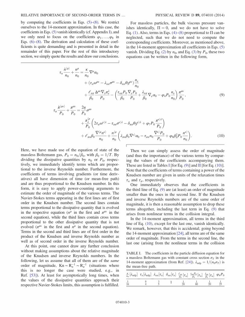
Then we can simply assess the order of magnitude(and thus the importance) of the various terms by compar-ing the values of the coefficients accompanying them.These are listed in Tables I [for Eq. (9)] and II [for Eq. (10)].Note that the coefficients of terms containing a power of theKnudsen number are given in units of the relaxation timesτn and τπ , respectively.One immediately observes that the coefficients in

the third line of Eq. (9) are (at least) an order of magnitudesmaller than the ones in the second line. If the Knudsenand inverse Reynolds numbers are of the same order ofmagnitude, it is then a reasonable assumption to drop theseterms altogether, including the last term in Eq. (9) thatarises from nonlinear terms in the collision integral.In the 14-moment approximation, all terms in the third

line of Eq. (10), except for the last one, vanish identically.We remark, however, that this is accidental; going beyondthe 14-moment approximation [24], all terms are of the sameorder of magnitude. From the terms in the second line, thelast one (arising from the nonlinear terms in the collision

TABLE I. The coefficients in the particle diffusion equation fora massless Boltzmann gas with constant cross section σT in the14-moment approximation (from Ref. [24]). λmfp ¼ 1=ðn0σTÞ isthe mean-free path.

κn0½λmfp� τn½λmfp� λnn½τn� δnn½τn� lnπ

β0½τn� τnπP0

β0½τn� λnπ

β0½τn� φ4P0

316

94

35

1 120

180

120

125

RELATIVE IMPORTANCE OF SECOND-ORDER TERMS IN … PHYSICAL REVIEW D 89, 074010 (2014)

074010-3

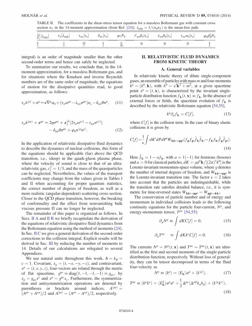
integral) is an order of magnitude smaller than the othersecond-order terms and hence can safely be neglected.To summarize our results, we conclude that, in the 14-

moment approximation, for a massless Boltzmann gas, andfor situations where the Knudsen and inverse Reynoldsnumbers are of the same order of magnitude, the equationsof motion for the dissipative quantities read, to goodapproximation, as follows:

τn _nhμi þnμ≃κ∇μα0þðτnωμν−λnnσμνÞnν−δnnθnμ; (11)

τπ _πhμνi þ πμν ≃ 2ησμν þ πhμλ ð2τπωνiλ − τππσ

νiλÞ− δππθπ

μν þ φ8nhμnνi: (12)

In the application of relativistic dissipative fluid dynamicsto describe the dynamics of nuclear collisions, this form ofthe equations should be applicable (far) above the QCDtransition, i.e., (deep) in the quark-gluon plasma phase,where the velocity of sound is close to that of an ultra-relativistic gas, c2s ¼ 1=3, and the mass of the quasiparticlescan be neglected. Nevertheless, the values of the transportcoefficients may change from the values given in Tables Iand II when accounting for proper quantum statistics,the correct number of degrees of freedom, as well as amore realistic (angular-dependent) scattering cross section.Closer to the QCD phase transition, however, the breakingof conformality and the effect from nonvanishing bulkviscous pressure Π can no longer be neglected.The remainder of this paper is organized as follows. In

Secs. II A and II B we briefly recapitulate the derivation ofthe equations of relativistic dissipative fluid dynamics fromthe Boltzmann equation using the method of moments [24].In Sec. II C we give a general derivation of the second-ordercorrections to the collision integral. Explicit results will bederived in Sec. III by reducing the number of moments to14. Details of our calculations are relegated to severalAppendices.We use natural units throughout this work, ℏ ¼ kB ¼

c ¼ 1. Covariant, xμ ¼ ðt;−x;−y;−zÞ, and contravariant,xμ ¼ ðt; x; y; zÞ, four-vectors are related through the metricof flat spacetime, gμν ≡ diagð1;−1;−1;−1Þ≡ gμν, byxμ ¼ gμνxν and xμ ¼ gμνxν. Furthermore, the symmetriza-tion and antisymmetrization operations are denoted byparentheses or brackets around indices, AðμνÞ ¼ðAμν þ AνμÞ=2 and A½μν� ¼ ðAμν − AνμÞ=2, respectively.

II. RELATIVISTIC FLUID DYNAMICSFROM KINETIC THEORY

A. General variables

In relativistic kinetic theory of dilute single-componentgases, anensembleofparticleswithmassm and four-momentakμ ¼ ðk0;kÞ, with k0 ¼

ffiffiffiffiffiffiffiffiffiffiffiffiffiffiffiffiffik2 þm2

p, at a given spacetime

point xμ ¼ ðt;xÞ, is characterized by the invariant single-particle distribution function fkðt;xÞ≡ fk. In the absence ofexternal forces or fields, the spacetime evolution of fk isdescribed by the relativistic Boltzmann equation [54,55],

kμ∂μfk ¼ C½f�; (13)

where C½f� is the collision term. In the case of binary elasticcollisions it is given by

C½f�¼1

ν

ZdK0dPdP0Wkk0→pp0ðfpfp0 ~fk ~fk0−fkfk0 ~fp ~fp0Þ:

(14)

Here ~fk ¼ 1 − afk, with a ¼ 1ð−1Þ for fermions (bosons)and a ¼ 0 for classical particles, dK ¼ gd3k=½ð2πÞ3k0� is theLorentz-invariant momentum-space volume, where g denotesthe number of internal degrees of freedom, and Wkk0→pp0 isthe Lorentz-invariant transition rate. The factor ν ¼ 2 takesinto account that the particles are indistinguishable, whilethe transition rate satisfies detailed balance, i.e., it is sym-metric for time-reversed states Wkk0→pp0 ¼ Wpp0→kk0.The conservation of particle number and of energy and

momentum in individual collisions leads to the followingcontinuity equations for the particle four-current, Nμ, andenergy-momentum tensor, Tμν [54,55]:

∂μNμ ≡Z

dKC½f� ¼ 0; (15)

∂μTμν ≡Z

dKkνC½f� ¼ 0: (16)

The currents Nμ ¼ Nμðt;xÞ and Tμν ¼ Tμνðt;xÞ are iden-tified as the first and second moments of the single-particledistribution function, respectively. Without loss of general-ity, they can be tensor decomposed in terms of the fluidfour-velocity as

Nμ ≡ hkμi ¼ hEkiuμ þ hkhμii; (17)

Tμν ≡ hkμkνi ¼ hE2kiuμuν þ

1

3ΔμνhΔαβkαkβi þ hkhμkνii;

(18)

TABLE II. The coefficients in the shear-stress tensor equation for a massless Boltzmann gas with constant crosssection σT in the 14-moment approximation (from Ref. [24]). λmfp ¼ 1=ðn0σTÞ is the mean-free path.

2ηP0½λmfp� τπ½λmfp� τππ½τπ� δππ ½τπ� φ7P0 lπnβ0½τπ� λπnβ0½τπ� τπnn0½τπ� φ8β

20P0

83

53

107

43

970

0 0 0 85


074010-4

where h� � �i ¼ R dKð� � �Þfk. Here, Ek ¼ kμuμ and khμi ¼Δμνkν correspond to the energy and the three-momentum,respectively, of the particle in the local rest frame ofthe fluid, such that kμ ¼ Ekuμ þ khμi [23,24,56–58].Moreover, we denoted the orthogonal projection of afirst-rank tensor as Ahμi ≡ ΔμνAν, while the symmetric,traceless, and orthogonal projection of second-rank tensorsAμν is defined as Ahμνi ≡ Δμν

αβAαβ, with Δμναβ ¼

ðΔμαΔβν þ ΔναΔβμÞ=2 − ΔμνΔαβ=3. In this work, the flowvelocity uμ is defined according to the Landau prescription[13] as the eigenvector of the energy-momentum tensor,i.e., Tμνuν ¼ hE2

kiuμ. As a consequence, the energy-momentum diffusion current vanishes,Wμ ≡ hEkkhμii ¼ 0.Using Eqs. (17)–(18) we are able to identify the

fundamental fluid-dynamical quantities as

n≡ Nμuμ ¼ hEki; (19)

ε≡ Tμνuμuν ¼ hE2ki; (20)

P≡− 1

3TμνΔμν ¼ − 1

3hΔαβkαkβi; (21)

nμ ≡ NνΔμν ¼ hkhμii; (22)

πμν ≡ TαβΔμναβ ¼ hkhμkνii; (23)

where n is the particle number density, ε is the energydensity, P is the local isotropic pressure, nμ is the particlediffusion current, and πμν is the shear-stress tensor.It is customary to separate the isotropic pressure into

two components, P ¼ P0 þ Π, with P0 being thethermodynamic pressure and Π the bulk viscous pres-sure. The thermodynamic and bulk viscous pressures aredefined with respect to the local equilibrium distributionfunction,

f0k ¼ ½expðβ0Ek − α0Þ þ a�−1; (24)

and

P0 ¼ − 1

3hΔαβkαkβi0; (25)

Π ¼ − 1

3hΔαβkαkβiδ; (26)

where h� � �i0 ¼RdKð� � �Þf0k and h� � �iδ ¼

RdKð� � �Þδfk,

with δfk ≡ fk − f0k. The temperature and chemicalpotential, μ ¼ Tα0, introduced in f0k are defined bythe so-called matching conditions which impose that theparticle number density and energy density are given bytheir respective values in a fictitious local thermody-namic equilibrium state, i.e., n0 ≡ hEki0 ¼ n andε0 ≡ hE2

ki0 ¼ ε. In this state, there is an equation ofstate of the form P0ðT; μÞ, such that n0 ¼ ∂P0=∂μ,

s0 ¼ ∂P0=∂T, and the fundamental thermodynamicalrelation ε0 ¼ Ts0 þ μn0 − P0 is fulfilled.It is also convenient to introduce the irreducible

moments of δfk,

ρμ1…μlr ¼ hEr

kkhμ1…kμliiδ: (27)

Such irreducible moments are constructed to be symmetric,traceless, and orthogonal to the four-velocity, with the sym-metrized,traceless,andorthogonalprojectionsbeingdefinedas

khμ1 :::::kμli ¼ Δμ1…μlν1…νl k

ν1…kνl : (28)

Thedetails of construction and the properties of such tensorscan be found in Appendix B. Note that the bulk viscouspressure, particle diffusion current, and shear-stress tensor arealso irreducible moments of δfk,

Π ¼ −m2

3ρ0; nμ ¼ ρμ0; πμν ¼ ρμν0 : (29)

Furthermore, the matching conditions and the definition ofthe local rest frame can also be expressed using irreduciblemoments. The matching conditions correspond to

ρ1 ≡ hEkiδ ¼ 0; (30)

ρ2 ≡ hE2kiδ ¼ 0; (31)

while the Landau definition of the fluid four-velocity leads to

ρμ1 ≡ hkhμiEkiδ ¼ 0: (32)

B. Moment expansion of fk and the equations ofmotion for the irreducible moments

Following Ref. [24], δfk is parametrized as

δfk ¼ f0k ~f0kϕk: (33)

The function ϕk is then expanded in terms of a series in theirreducible tensors given in Eq. (28),

ϕk ¼X∞l¼0

λhμ1…μlik khμ1…kμli: (34)

By expanding the tensor λhμ1…μlik using a set of orthogonal

polynomials, it is straightforward to prove that

λhμ1…μlik ¼

XNl

n¼0

HðlÞkn ρ

μ1…μln ; (35)

where Nl denotes the order at which the expansion istruncated (for the coefficient of rank l) and ρμ1:::::μln is theirreducible moment defined in Eq. (27). The coefficientsHðlÞ

kn are found to be [24]


074010-5

HðlÞkn ¼ WðlÞ

l!

XNl

m¼n

aðlÞmnPðlÞkm; (36)

with PðlÞkm being orthogonal polynomials in Ek,

PðlÞkm ¼

Xmr¼0

aðlÞmrErk: (37)

The coefficients aðlÞmr are determined from the orthonor-mality conditionZ

dKωðlÞPðlÞkmP

ðlÞkn ¼ δmn; (38)

using Gram-Schmidt orthogonalization. The measure ωðlÞdepends on the rank l of the tensor being expanded and reads

ωðlÞ ¼ WðlÞ

ð2lþ 1Þ!! ðΔαβkαkβÞlf0k ~f0k; (39)

where WðlÞ is a normalization constant defined as

WðlÞ ¼ ð−1ÞlðJ2l;lÞ−1: (40)

For more details, see Refs. [24,25].Using the Boltzmann equation, one can derive the

general equations of motion satisfied by ρμ1:::::μlr . This isaccomplished by explicitly taking the comoving derivativeof the corresponding irreducible moment, i.e.,_ρhμ1…μlir ¼ Δμ1…μl

ν1…νlDRdKEr

kkhν1…kνliδfk, and using the

Boltzmann equation to express the comoving derivative ofδfk in terms of the collision term, f0k and its derivatives,and spatial derivatives of δfk. The details of this derivationas well as the general form of the resulting equationsof motion are contained in Refs. [24,25]. For the threelowest-rank moments, these equations of motion read

_ρr − Cr−1 ¼ αð0Þr θ þ ðnonlinear termsÞ; (41)

_ρhμir − Chμir−1 ¼ αð1Þr Iμ þ ðnonlinear termsÞ; (42)

_ρhμνir − Chμνir−1 ¼ 2αð2Þr σμν þ ðnonlinear termsÞ: (43)

Here we define the following thermodynamic quantities:

αð0Þr ¼ ð1 − rÞIr1 − Ir0 − n0D20

ðh0G2r −G3rÞ; (44)

αð1Þr ¼ Jrþ1;1 − h−10 Jrþ2;1; (45)

αð2Þr ¼ Irþ2;1 þ ðr − 1ÞIrþ2;2; (46)

where h0 ¼ ðε0 þ P0Þ=n0 denotes the enthalpy per particleand

Gnm ¼ Jn0Jm0 − Jn−1;0Jmþ1;0; (47)

Dnq ¼ Jnþ1;qJn−1;q − ðJnqÞ2: (48)

The variables Inþr;qðα0; β0Þ and Jnþr;qðα0; β0Þ correspondto thermodynamic integrals defined as

Irþn;q ¼ð−1Þq

ð2qþ 1Þ!! hEnþr−2qk ðΔαβkαkβÞqi0; (49)

Jrþn;q ¼∂Inþr;q

∂α0��β0

: (50)

More details can be found in Appendix A.We also introduced the generalized irreducible collision

integral Cμ1:::::μlr and its symmetric, traceless, and orthogo-

nal projection,

Chμ1…μlir ≡ Δμ1…μl

ν1…νlCν1…νlr ¼

ZdKEr

kkhμ1…kμliC½f�:

(51)

Aswas shown inRef. [24], themoment equations (41)–(43)reduce to the fluid-dynamical equations for the dissipativevariables when the fast-varying modes of the Boltzmannequation can be neglected and, simultaneously, the Knudsennumber(s) and inverse Reynolds number(s) are small. In thiscase, the linear parts of the collision integrals introducedabove determine the relaxation times for the dissipativevariables, while their nonlinear parts give rise to the termsthat are of second order in the inverse Reynolds number(s),i.e., the tensors R, Rμ, and Rμν that appear in Eqs. (6)–(8).In Ref. [24] the existence of such nonlinear terms waspointed out, but the explicit calculation of the correspondingtransport coefficients was left for future work. In the nextsections we shall complete this task.

C. Expansion of the collision integral

In this section we show how to express the collisionintegrals in terms of irreducible moments of δfk.Substituting the expression of the collision term for binaryelastic collisions (14) into the expression for the irreduciblecollision integral (51), one obtains

Chμ1…μlir−1 ¼ 1

ν

ZdKdK0dPdP0Wkk0→pp0Er−1

k khμ1 :::::kμli

× ðfpfp0 ~fk ~fk0 − fkfk0 ~fp ~fp0 Þ: (52)

Substituting the distribution function fk ¼ f0k þf0k ~f0kϕk into the above formula and using

fpfp0 ¼ f0pf0p0 ð1þ ~f0p0ϕp0 þ ~f0pϕpÞþ f0pf0p0 ~f0p ~f0p0ϕpϕp0 ; (53)


074010-6

~fp ~fp0 ¼ ~f0p ~f0p0 ð1 − af0p0ϕp0 − af0pϕpÞþ a2f0pf0p0 ~f0p ~f0p0ϕpϕp0 ; (54)

together with the equality f0kf0k0 ~f0p ~f0p0 ¼f0pf0p0 ~f0k ~f0k0 , the part that is linear in ϕk reads

Lhμ1:::::μlir−1 ¼ 1

ν

ZfEr−1k khμ1 :::::kμliðϕp þ ϕp0 − ϕk − ϕk0 Þ;

(55)

where we abbreviatedRf ¼

RdKdK0dPdP0Wkk0→pp0

f0kf0k0 ~f0p ~f0p0 and used the fact that the collision termvanishes for the local equilibrium distribution functionCμ1…μlr ½f0� ¼ 0. Inserting the expression for ϕk from the

moment expansion (34) into the previous equation, weobtain

Lhμ1:::::μlir−1 ¼ 1

ν

X∞m¼0

XNm

n¼0

ZfEr−1k khμ1 :::::kμliρν1…νm

n

× ðHðmÞpn phν1…pνmi þHðmÞ

p0n p0hν1…p0

νmi

−HðmÞkn khν1…kνmi −HðmÞ

k0nk0hν1…k0νmiÞ: (56)

It was shown in Ref. [24] that the linear part of thecollision integral simplifies to

Lhμ1…μlir−1 ¼

X∞m¼0

XNm

n¼0

ðArnÞμ1…μlν1…νmρ

ν1…νmn

¼X∞m¼0

XNm

n¼0

AðlÞrn ρ

μ1…μln ; (57)

where

ðArnÞμ1…μlν1…νm ¼ 1

ν

ZfEr−1k khμ1…kμli

× ðHðmÞpn phν1…pνmi þHðmÞ

p0n p0hν1…p0

νmi

−HðmÞkn khν1…kνmi −HðmÞ

k0nk0hν1…k0νmiÞ: (58)

While using the properties of the irreducible projectiontensors, one can show that

AðlÞrn ¼ ½Δα1…αl

α1…αl �−1Δν1…νlμ1…μlðArnÞμ1…μl

ν1…νl : (59)

The coefficient AðlÞrn is the (rn) element of a ðNl þ 1Þ ×

ðNl þ 1Þ matrix, AðlÞ, and, in the linearized case, containsall the information of the underlying microscopic theory.We remark that, for l ¼ 0, the second and third rows andcolumns (r, n ¼ 1, 2) and, for l ¼ 1, the second row andcolumn (r, n ¼ 1) are zero, because the moments ρ1, ρ2,and ρμ1 vanish due to the matching conditions and ourchoice of frame.The computation of the nonlinear part of the collision

integral is analogous. Inspecting the previous formulas weobserve that the collision integral is a quartic function ofϕk. However, in this paper we shall restrict our calculationsto the case of Boltzmann statistics (a ¼ 0), in which casethe dependence on ϕk becomes quadratic. The collisionintegral can be written as

Chμ1…μlir−1 ¼ Lhμ1…μli

r−1 þ Nhμ1…μlir−1 ; (60)

where the quadratic contribution to the collisionintegral reads

Nhμ1…μlir−1 ≡ 1

ν

ZfEr−1k khμ1…kμliðϕpϕp0 − ϕkϕk0 Þ

¼ 1

ν

X∞m;m0¼0

XNm

n¼0

XNm0

n0¼0

ZfEr−1k khμ1…kμliρα1…αm

n ρβ1…βm0n0

× ðHðmÞpn Hðm0Þ

p0n0 phα1…pαmip0hβ1…p0

βm0 i −HðmÞkn H

ðm0Þk0n0 khα1 :::::kαmik

0hβ1 :::::k

0βm0 iÞ: (61)

This nonlinear contribution can be further simplified to

Nhμ1…μlir−1 ¼

X∞m0¼0

Xm0

m¼0

XNm

n¼0

XNm0

n0¼0

ðN rnn0 Þμ1…μlα1…αmβ1…βm0ρ

α1…αmn ρ

β1…βm0n0 ; (62)

where we defined the following tensor of rank lþmþm0:


074010-7

ðN rnn0 Þμ1…μlα1…αmβ1…βm0 ¼

1

ν

ZfEr−1k khμ1…kμli

× ½HðmÞpn Hðm0Þ

p0n0 phα1…pαmip0hβ1…p0

βm0 i þ ð1 − δmm0 ÞHðmÞp0nH

ðm0Þpn0 p

0hα1…p0

αmiphβ1…pβm0 i

−HðmÞkn H

ðm0Þk0n0 khα1…kαmik

0hβ1…k0βm0 i − ð1 − δmm0 ÞHðmÞ

k0nHðm0Þkn0 k

0hα1…k0αmikhβ1…kβm0 i�: (63)

In comparison with Eq. (61), we have split the double sumP∞m¼0

P∞m0¼0

into a double sumP∞

m0¼0

Pm0m¼0 and a double

sumP∞

m¼0

Pmm0¼0

, and subtracted the superfluous termm ¼m0 in the last sum with the help of a Kronecker delta. Thenwe interchanged indices m↔m0, n↔n0 in the second sum.The tensor ðN rnn0 Þμ1…μl

α1…αmβ1…βm0 is symmetric under per-mutations of μ—type, α—type, and β—type indices, anddepends solely on equilibrium distribution functions andthe corresponding cross section(s). The equilibrium dis-tribution function contains only one four-vector, i.e., thefluid four-velocity uμ. Therefore, ðN rnn0 Þμ1…μl

α1…αmβ1…βm0 mustbe constructed from tensor structures made of uμ and themetric tensor gμν, or, equivalently, uμ andΔμν. Furthermore,ðN rnn0 Þμ1…μl

α1…αmβ1…βm0 must be orthogonal to uμ, whichimplies that it can only be constructed from combinationsof elementary projection operators, Δμν. This alreadyconstrains the rank of the tensor, lþmþm0, to be aneven number. Finally, it must satisfy the following property:

Δμ01…μ0l

μ1…μlΔα1…αmα01…α0m

Δβ1…βm0β01…β0

m0ðN rnn0 Þμ1…μl

α1…αmβ1…βm0

¼ ðN rnn0 Þμ01…μ0l

α01…α0mβ01…β0

m0: (64)

For our purposes it is sufficient to calculate terms that areof second order in the inverse Reynolds number, i.e., thetermsR,Rμ, andRμν. Therefore, we only need to considerthe cases l ¼ 0, l ¼ 1, and l ¼ 2. Since the actualdeduction of the nonlinear collision integrals is compli-cated, this task is relegated to Appendix C and here we shallonly give the final results.The scalar nonlinear collision integral from Eq. (62) is

given by

Nr−1 ≡X∞m0¼0

Xm0

m¼0

XNm

n¼0

XNm0

n0¼0

ðN rnn0 Þα1…αmβ1…βm0ρα1…αmn ρ

β1…βm0n0

¼XN0

n¼0

XN0

n0¼0

C0ð0;0Þrnn0 ρnρn0

þX∞m¼1

XNm

n¼0

XNm

n0¼0

C0ðm;mÞrnn0 ρα1…αm

n ρn0;α1…αm; (65)

where C0ðm;mÞrnn0 is the special case l ¼ 0 of a more general

coefficient

Clðm;mþlÞrnn0 ¼ 1

ð2mþ 2lþ 1ÞνZfEr−1k khμ1 :::::kμli½HðmÞ

pn HðmþlÞp0n0 phν1…pνmip0

hμ1…p0μlp

0ν1…p0

νmi

þð1 − δm;mþlÞHðmÞp0nH

ðmþlÞpn0 p0hν1…p0νmiphμ1…pμlpν1…pνmi

−HðmÞkn H

ðmþlÞk0n0 khν1…kνmik0hμ1…k0μlk

0ν1…k0νmi

− ð1 − δm;mþlÞHðmÞk0nH

ðmþlÞkn0 k0hν1…k0νmikhμ1…kμlkν1…kνmi�: (66)

Similarly, the nonlinear collision term for l ¼ 1 becomes,

Nμr−1 ≡

X∞m0¼0

Xm0

m¼0

XNm

n¼0

XNm0

n0¼0

ðN rnn0 Þμα1…αmβ1…βm0ρα1…αmn ρ

β1…βm0n0

¼XN0

n¼0

XN1

n0¼0

C1ð0;1Þrnn0 ρnρμn0 þ

X∞m¼1

XNm

n¼0

XNmþ1

n0¼0

C1ðm;mþ1Þrnn0 ρα1…αm

n ρμn0;α1…αm; (67)

where the coefficient C1ðm;mþ1Þrnn0 is the l ¼ 1 case of the general coefficient Clðm;mþlÞ

rnn0 introduced in Eq. (66).


074010-8

Finally, the rank-2 tensor terms are obtained takingl ¼ 2,

Nμνr−1 ≡

X∞m0¼0

Xm0

m¼0

XNm

n¼0

XNm0

n0¼0

ðN rnn0 Þμνα1…αmβ1…βm0ρα1…αmn ρ

β1…βm0n0

¼X∞m¼0

XNmþ2

n¼0

XNm

n0¼0

C2ðm;mþ2Þrnn0 ρα1…αm

n ρμνn0;α1…αm

þXN1

n¼0

XN1

n0¼0

D2ð11Þrnn0 ρ

hμn ρ

νin0

þX∞m¼2

XNm

n¼0

XNm

n0¼0

D2ðmmÞrnn0 ρα2…αmhμ

n ρνin0;α2…αm; (68)

where C2ðm;mþ2Þrnn0 can be calculated from Eq. (66); we

introduce another coefficient,

D2ðmmÞrnn0 ¼ 1

dðmÞν

ZfEr−1k khμkνi

× ðHðmÞpn HðmÞ

p0n0phμpβqþ1…pβmip0hνp

0βqþ1

…p0βmi

−HðmÞkn H

ðmÞk0n0khμk

βqþ1…kβmik0hνkβqþ1…k0βmiÞ: (69)

The normalization dðmÞ is complicated and is discussedin Appendix C together with other details of the derivationof the nonlinear collision term.

III. TRANSPORT COEFFICIENTS IN THE14–MOMENT APPROXIMATION

In this section we calculate the previously introduced

coefficients AðlÞrn , C

0ðmmÞrnn0 , C1ðm;mþ1Þ

rnn0 , C2ðm;mþ2Þrnn0 , and D2ðm;mÞ

rnn0

in the 14–moment approximation. As shown inRefs. [24,25], this corresponds to the truncation N0 ¼ 2,N1 ¼ 1,N2 ¼ 0. This implies that the following irreduciblemoments appear: ρ0 ¼ −3Π=m2, ρ1 ¼ 0, ρ2 ¼ 0, ρμ0 ¼ nμ,ρμ1 ¼ 0, and ρμν0 ¼ πμν. As one can see, they are uniquelyrelated to the dissipative quantities.Before proceeding and for the sake of later convenience,

we reexpress the coefficients HðlÞkn using Eqs. (36) and (37)

as

HðlÞkn ≡WðlÞ

l!

XNl

k¼n

Xkr¼0

aðlÞkr aðlÞkn E

rk

¼XNl

r¼n

AðlÞrn Er

k þXn−1r¼0

AðlÞnr Er

k; (70)

where

AðlÞrn ¼ WðlÞ

l!

XNl

k¼r

aðlÞkr aðlÞkn : (71)

Note that, for n ¼ 0, the second sum in Eq. (70) identicallyvanishes, which greatly simplifies the calculation of thecollision integral.Furthermore, from the definition of the irreducible

moments and using Eqs. (34)–(37) together with theorthogonality condition (B8) we obtain the followinggeneral result:

ρμ1:::::μlr ≡ l!ð2lþ 1Þ!!

XNl

n¼0

ρμ1:::::μln

×Z

dKErkðΔαβkαkβÞlHðlÞ

kn f0k ~f0k

¼ ð−1Þll!XNl

n¼0

ρμ1:::::μln

×

XNl

r0¼n

AðlÞr0nJrþr0þ2l;l þ

Xn−1r0¼0

AðlÞnr0 Jrþr0þ2l;l

!;

(72)

where we used Eq. (70) in the last step. Therefore,truncating the above general result in the 14–momentapproximation we obtain

ρr ≡ γΠr ρ0 ¼ − 3

m2ðAð0Þ

00 Jr;0 þ Að0Þ10 Jrþ1;0 þ Að0Þ

20 Jrþ2;0ÞΠ;(73)

ρμr ≡ γnrρμ0 ¼ −ðAð1Þ

00 Jrþ2;1 þ Að1Þ10 Jrþ3;1Þnμ; (74)

ρμνr ≡ γπrρμν0 ¼ ð2Að2Þ

00 Jrþ4;2Þπμν; (75)

where for r ¼ 0 we obviously have γΠ0 ¼ γn0 ¼ γπ0 ¼ 1. The

coefficients Að0Þ20 , A

ð1Þ10 , A

ð2Þ00 , as well as A

ð0Þ00 , A

ð0Þ10 , A

ð0Þ20 , are

calculated from Eq. (71) and listed in Appendix D. Theselinear relations between the moments are the main result ofthe 14–moment approximation, which was also obtainedin Ref. [25].It is straightforward to show using Eqs. (58), (59), and

(70) that the AðlÞrn coefficients of the linear collision term

can be expressed in terms of AðlÞrn . For l ¼ 0 where, in the

14–moment approximation, N0 ¼ 2, the coefficient is

Að0Þr0 ≡ Að0Þ

20

1

ν

ZfEr−1k ðE2

p þ E2p0 − E2

k − E2k0 Þ

¼ Að0Þ20 X

μναβðr−3Þuμuνuαuβ; (76)

where the integrals proportional to Að0Þ00

Rf ð1þ 1 − 1−

1Þ ¼ 0 and Að0Þ10

Rf ðEp þ Ep0 − Ek − Ek0 Þ ¼ 0 vanish

due to particle number and energy conservation in binarycollisions. Here, we introduce the rank-4 tensor


074010-9

XμναβðrÞ ¼ 1

ν

ZfErkk

μkνðpαpβ þ p0αp0β − kαkβ − k0αk0βÞ;

(77)

which is symmetric upon the interchange of indices ðμ; νÞand ðα; βÞ, i.e., Xμναβ

ðrÞ ¼ XðμνÞðαβÞðrÞ , and it is also traceless in

the latter indices, XμναβðrÞ gαβ ¼ 0.

Similarly, for l ¼ 1 we have

Að1Þr0 ≡ Að1Þ

10

1

3ν

ZfEr−1k khμi

× ðEpphμi þ Ep0p0hμi − Ekkhμi − Ek0k0hμiÞ

¼ Að1Þ10

1

3Xμναβðr−2ÞuðμΔνÞðαuβÞ; (78)

where Að1Þ00

Rf ðphμi þ p0

hμi − khμi − k0hμiÞ ¼ 0 vanishes dueto three-momentum conservation.Finally, for l ¼ 2 we obtain

Að2Þr0 ≡ Að2Þ

00

1

5ν

ZfEr−1k khμkνi

× ðphμpνi þ p0hμp

0νi − khμkνi − k0hμk

0νiÞ

¼ Að2Þ00

1

5Xμναβðr−1ÞΔμναβ: (79)

Recalling that Lhμ1:::::μlir−1 ¼PNl

n¼0AðlÞrn ρ

μ1:::::μln , these results

lead to the linear collision terms in the 14–momentapproximation,

Lr−1 ¼X2n¼0

Að0Þrn ρn ≡Að0Þ

r0 ρ0 ¼ −Að0Þ20 Xðr−3Þ;1

3

m2Π; (80)

Lhμir−1 ¼

X1n¼0

Að1Þrn ρ

μn ≡Að1Þ

r0 ρμ0 ¼ Að1Þ

10 Xðr−2Þ;3nμ; (81)

Lhμνir−1 ¼ Að2Þ

r0 ρμν0 ¼ Að2Þ

00 Xðr−1Þ;4πμν: (82)

Here, we denote the different tensor projections asXðrÞ;1 ¼ Xμναβ

ðrÞ uμuνuαuβ, XðrÞ;3 ¼ 13XμναβðrÞ uðμΔνÞðαuβÞ, and

XðrÞ;4 ¼ 15XμναβðrÞ Δμναβ.

Now, with the help of these formulas and usingEqs. (73)–(75), the coefficients of bulk viscosity, particlediffusion, and shear viscosity, as well as the correspondingrelaxation times can be calculated,

ζr ¼ αð0Þr

Að0Þ20 Xðr−3Þ;1

; τrΠ ¼ − γΠr


; (83)

κr ¼ − αð1Þr


; τrn ¼ − γnr


; (84)

ηr ¼ − αð2Þr


; τrπ ¼ − γπr


; (85)

where αð0Þr , αð1Þr , and αð2Þr were defined in Eqs. (44)–(46)while γΠr , γnr , and γπr are listed in Eqs. (73)–(75).We now compute the nonlinear collision terms. With

Eq. (70), the scalar contribution (66) is

C0ðmmÞrnn0 ¼ 1

ð2mþ 1ÞνZfEr−1k

×

��XNm

i¼n

AðmÞin Ei

p þXn−1i¼0

AðmÞni Ei

p

��XNm

i0¼n0AðmÞi0n0 E

i0p0 þ

Xn0−1i0¼0

AðmÞn0i0 E

i0p0

�phμ1 :::::pμmip0

hμ1 :::::p0μmi

−�XNm

i¼n

AðmÞin Ei

k þXn−1i¼0

AðmÞni Ei

k

��XNm

i0¼n0AðmÞi0n0 E

i0k0 þ

Xn0−1i0¼0

AðmÞn0i0 E

i0k0

�khμ1 :::::kμmik0hμ1 :::::k

0μmi

�: (86)

As noted before, in the 14–moment approximation termsproportional to

Pn−1i¼0 A

ðmÞni vanish, hence Eq. (65) leads to

Nr−1 ¼9

m4C0ð00Þr00 Π2 þ C0ð11Þr00 nμnμ þ C0ð22Þr00 πμνπμν; (87)

where we used Eqs. (73)–(75) for the ρα1:::::αmn ’s. Thecoefficients in the above equation are

C0ð00Þr00 ¼ ðAð0Þ10 Þ2Y2ðr−3Þ;1 þ ðAð0Þ

20 Þ2Y5ðr−3Þ;1þ ðAð0Þ

00 Að0Þ20 ÞXðr−3Þ;1 þ ðAð0Þ

10 Að0Þ20 ÞY3ðr−3Þ;1; (88)

C0ð11Þr00 ¼ − 1

3ðAð1Þ

00 Þ2Y2ðr−3Þ;1 þ ðAð1Þ00 A

ð1Þ10 ÞY3ðr−3Þ;5

þ ðAð1Þ10 Þ2Y5ðr−3Þ;5; (89)


074010-10

C0ð22Þr00 ¼ 2ðAð2Þ00 Þ2Y5ðr−3Þ;9; (90)

where the detailed derivation is given in Appendix E.Comparing the above result to Eq. (6) and taking intoaccount the corresponding relaxation time from Eq. (1), weobtain

φ1 ¼9

m4

τrΠγΠr

C0ð00Þr00 ; (91)

φ2 ¼τrΠγΠr

C0ð11Þr00 ; (92)

φ3 ¼τrΠγΠr

C0ð22Þr00 : (93)

Similarly, the vector term (67) in the 14–momentapproximation leads to the following formula:

Nμr−1 ¼ C1ð12Þr00 nνπμν − 3

m2C1ð01Þr00 Πnμ; (94)

where

C1ð12Þr00 ¼ 2½ðAð1Þ00 A

ð2Þ00 ÞY3ðr−2Þ;8 þ ðAð1Þ

10 Að2Þ00 ÞY4ðr−2Þ;8�; (95)

C1ð01Þr00 ¼ ðAð0Þ00 A

ð1Þ10 ÞXðr−2Þ;3 þ ðAð0Þ

10 Að1Þ00 ÞY1ðr−2Þ;3

þ ðAð0Þ10 A


− ðAð0Þ20 A

ð1Þ00 Þð3Y3ðr−2Þ;6 þ 2Y3ðr−2Þ;8Þ

þ ðAð0Þ20 A

ð1Þ10 ÞY4ðr−2Þ;3: (96)

Now, recalling Eq. (7) we obtain

φ4 ¼τrnγnr

C1ð12Þr00 ; (97)

φ5 ¼ − 3

m2

τrnγnr

C1ð01Þr00 : (98)

Finally, the tensor term (68) is

Nμνr−1 ¼ − 3

m2C2ð0;2Þr00 Ππμν þD2ð2;2Þ

r00 πλhμπνiλ þD2ð1;1Þr00 nhμnνi;

(99)

where

C2ð02Þr00 ¼ Að2Þ00 ½Að0Þ

00 Xðr−1Þ;4 þ Að0Þ10 Y3ðr−1Þ;4 þ Að0Þ

20 Y4ðr−1Þ;4�;(100)

D2ð22Þr00 ¼ 8ðAð2Þ

00 Þ2Y5ðr−1Þ;11; (101)

D2ð11Þr00 ¼ ðAð1Þ

00 Þ2Y2ðr−1Þ;4 þ 2ðAð1Þ00 A


þ 2ðAð1Þ10 Þ2Y5ðr−1Þ;7; (102)

and a comparison with Eq. (8) yields

φ6 ¼ − 3

m2

τrπγπr

C2ð0;2Þr00 ; (103)

φ7 ¼τrπγπr

D2ð2;2Þr00 ; (104)

φ8 ¼τrπγπr

D2ð1;1Þr00 : (105)

In order to calculate these coefficients we introduce fivenew tensors, which are similar to Xμναβ

ðrÞ and are given asfollows:

Yμναβ1ðrÞ ¼ 1

ν

ZfErkk

μkνðpαp0β þ p0αpβ − kαk0β − k0αkβÞ;

(106)

Yμναβ2ðrÞ ¼ 1

ν

ZfErkk

μkν½pαp0β − kαk0β�; (107)

Yμναβκ3ðrÞ ¼ 1

ν

ZfErkk

μkνðpαp0βp0κ þ p0αpβpκ

− kαk0βk0κ − k0αkβkκÞ; (108)

Yμναβκλ4ðrÞ ¼ 1

ν

ZfErkk

μkνðpαpβp0κp0λ þ p0αp0βpκpλ

− kαkβk0κk0λ − k0αk0βkκkλÞ; (109)


ν

ZfErkk

μkνðpαpβp0κp0λ − kαkβk0κk0λÞ: (110)

Note that the YiðrÞ;j terms in the previous equations aredifferent contractions of these five tensors. Our notation issuch that the i index specifies the tensor while the j indexlabels a particular contraction. More details are given inAppendix F.We have shown earlier that the coefficients in the

equations of motion depend explicitly on the choice ofthe moment, i.e., the index r. Therefore, once the14–moment approximation is enforced, any moment ofthe Boltzmann equation leads to a closed set of equations,but when calculating the coefficients of the nonlinearcollision integrals one has to account for the exact form ofthe relaxation equations which follow from Eqs. (41)–(43)using Eqs. (73)–(75). As an examplewe quote the equationsfor the particle diffusion current and shear-stress tensorfor arbitrary r,


074010-11

τrn _nhμi þ nμ þ 3

m2

τrnC1ð01Þr00

γnrΠnμ − τrnC

1ð12Þr00

γnrnνπμν

¼ κr∇μα0 þ � � � ; (111)

τrππhμνi þ πμν þ 3

m2

τrπC2ð0;2Þr00

γπrΠπμν − τrπD

2ð2;2Þr00

γπrπλhμπνiλ

− τrπD2ð1;1Þr00

γπrnhμnνi ¼ 2ηrσμν þ � � � : (112)

Note that in order to recover Eqs. (1)–(3) one must taker ¼ 0, i.e., ζ ¼ ζ0, κ ¼ κ0, η ¼ η0, τΠ ¼ τ0Π, τn ¼ τ0nand τπ ¼ τ0π .Using the above relations, it was already shown in

Ref. [25] how to derive the equations of motion andcalculate the transport coefficients for different choicesof the moments corresponding to the traditional method byIsrael and Stewart [22] and to the one proposed by Denicol,Koide, and Rischke (DKR) [23]. Here, we shall follow thisrecipe and calculate the coefficients of the nonlinearcollision integral in both cases.The equations of motion derived by Israel and Stewart

[22] can be obtained by the choice ρ3 ¼ − 3m2 γΠ3Π,

ρμ2 ¼ γn2nμ, ρ1 ¼ γπ1π

μν in Eqs. (73)–(75) and substitutingthese values into the equations of motion (41)–(43).Therefore, in the IS theory all coefficients need to becalculated with r ¼ 3 for the scalar moments, r ¼ 2 forvector moments, and r ¼ 1 for second-rank tensormoments. In contrast, the choice of DKR is to use r ¼ 0for all equations and coefficients.We explicitly compute some of these coefficients in the

ultrarelativistic limit, mβ0 → 0, for a classical gas (a ¼ 0)with fixed cross section. Since in this limit Π ¼ 0, we donot need to compute the coefficients φ1, φ2, and φ3

appearing in the termR, Eq. (6), which enters the equationof motion (1) for the bulk viscous pressure. Furthermore,φ5, φ6 are coefficients in terms which are proportional toΠ,and thus also need not be computed. The remaining,nonvanishing coefficients corresponding to the DKRchoice r ¼ 0 are simply denoted as φ4, φ7, and φ8, whilethe ones corresponding to the IS choice are denoted by φIS

4

for r ¼ 2, while φIS7 and φIS

8 for r ¼ 1. They read

φ4 ¼1

25P−10 ; φIS

4 ¼ 1

4P−10 ; (113)

φ7 ¼9

70P−10 ; φIS

7 ¼ 1

5P−10 ; (114)

φ8 ¼8

5β20P−10 ; φIS

8 ¼ − 4

5β20P−10 : (115)

We observe that only φ8 (multiplying nhμnνi) differs in signbetween the DKR and IS choices, with the absolutemagnitude of the latter being half as large. The coefficients

φ7 (multiplying πλhμπνiλ ) are approximately of the samemagnitude for both choices, while φ4 (multiplying nνπμν) ismore than six times smaller in DKR than in IS theory. Theimplications of these results have already been discussed inthe Introduction and Conclusions for the DKR choice.Finally, for further reference, we also quote the coef-

ficients of particle diffusion and shear viscosity,

κ ¼ 3

16n0λmfp; κIS ¼ 1

8n0λmfp; (116)

η ¼ 4

3P0λmfp; ηIS ¼ 6

5P0λmfp; (117)

where λmfp ¼ 1=ðn0σTÞ is the mean-free path and σT isthe total cross section. Note that all remaining transportcoefficients from Eq. (4) were already computed inRef. [25] for both the DKR and IS choices and it wasshown that the differences are of the order of 10%–30%.Therefore, the only coefficients that change considerablyfrom one formalism to the other are φ4 and φ8.In closing we remark that the numerical solutions of both

the IS and DKR theories were compared to the numericalsolutions of the Boltzmann equation in various cases[23,53,59–62]. These investigations showed the advantagesof the DKR choice for the corresponding coefficients,which leads to a far better agreement with numericalsolutions of the Boltzmann equation than the IS theory.

ACKNOWLEDGMENTS

This work was supported by the Helmholtz InternationalCenter for FAIR within the framework of the LOEWEprogram launched by the State of Hesse. G. S. Denicol issupported by a Banting Fellowship of the Natural Sciencesand Engineering Research Council of Canada. The work ofH. Niemi was supported by Academy of Finland, ProjectNo. 133005. E. Molnár was partially supported by theEuropean Union and the European Social Fund throughproject Supercomputer, the national virtual lab (GrantNo. TAMOP-4.2.2.C-11/1/KONV-2012-0010), as well asby TAMOP 4.2.4. A/2-11-1-2012-0001 NationalExcellence Program (A2-MZPDÖ-13-0042). The authorsthank R. Paatelainen for his help with FeynCalc.

APPENDIX A: THERMODYNAMIC INTEGRALS

Following Refs. [22,28] we introduced the followingequilibrium moments of tensor rank n,

Iμ1:::::μnn ≡ hkμ1 :::::kμni0

¼X½n=2�q¼0

ð−1ÞqbnqInqΔðμ1μ2 :::::Δμ2q−1μ2quμ2qþ1 :::::uμnÞ;

(A1)


074010-12

where n, q are natural numbers and [n=2] is the largestinteger not exceeding n=2, cf. Eq. (A8) in Ref. [22]. Theparentheses ð…Þ around indices denote symmetrization.For an arbitrary tensor of rank n, this operation is definedby Aðμ1:::::μnÞ ¼ 1

n!

P℘μAμ1μ2:::::μn, where ℘μ denotes all

possible permutations of the μ indices.The bnq coefficient is equal to the number of permuta-

tions in the set ℘μ, which lead to identical tensor productsof the uμ and Δμν projectors [22],

bnq ≡ n!2qq!ðn − 2qÞ! ¼

n!ð2q − 1Þ!!ð2qÞ!ðn − 2qÞ! ; (A2)

see Eq. (A2) of Ref. [22].The thermodynamic integrals Inq and Jnq were defined

in Eqs. (49), (50),

Inq ¼ð−1Þq

ð2qþ 1Þ!!Z

dKðEkÞn−2qðΔαβkαkβÞqf0k; (A3)

Jnq ¼ð−1Þq

ð2qþ 1Þ!!Z

dKðEkÞn−2qðΔαβkαkβÞqf0k ~f0k: (A4)

Replacing ðΔαβkαkβÞq ¼ ðm2 − E2kÞq we get the following

recursion relations for 0 ≤ q ≤ n=2,

Inþ2;q ¼ m2In;q þ ð2qþ 3ÞInþ2;qþ1; (A5)

Jnþ2;q ¼ m2Jn;q þ ð2qþ 3ÞJnþ2;qþ1; (A6)

while an integration by parts of Eq. (A3) leads to thefollowing relation:

β0Jnq ¼ In−1;q−1 þ ðn − 2qÞIn−1;q: (A7)

Furthermore,

dInqðα0; β0Þ≡ ∂Inq∂α0 dα0 þ

∂Inq∂β0 dβ0;

¼ Jnqdα0 − Jnþ1;qdβ0; (A8)

with a similar relation for dJnqðα0; β0Þ.

APPENDIX B: IRREDUCIBLE TENSORS

We define the following projection operator [54]:

Δμ1:::::μnν1:::::νn ¼X½n=2�q¼0

cnqΦμ1:::::μnν1:::::νnðnqÞ ; (B1)

where the coefficients are given by

cnq ¼ ð−1Þq ðn!Þ2

ð2nÞ!ð2n − 2qÞ!

q!ðn − qÞ!ðn − 2qÞ! ; (B2)

and

Φμ1:::::μnν1:::::νnðnqÞ ¼ ðn − 2qÞ!

�2qq!n!

�2X℘μ℘ν

Δμ1μ2 :::::Δμ2q−1μ2q

× Δν1ν2 :::::Δν2q−1ν2qΔμ2qþ1ν2qþ1 :::::Δμnνn :

(B3)

The summation is taken over all distinct permutations ofμ- and ν-type indices (without mutual exchange of thesetypes of indices). The prefactor is the inverse of the numberof distinct permutations. This can be seen as follows: thetotal number of permutations of μ- and ν-type indices isðn!Þ2. In order to obtain the number of distinct permuta-tions, we have to divide this by the following threenumbers: ð2qÞ2 permutations lead to terms which onlydiffer by a trivial permutation of indices on the sameprojector, e.g. Δμ1μ2 ¼ Δμ2μ1 ; ðq!Þ2 terms just correspond toa pairwise exchange of indices between projectors, e.g.Δμ1μ2Δμ3μ4 ¼ Δμ3μ4Δμ1μ2 ; for any given distribution ofμ-type indices in the product Δμ2qþ1ν2qþ1 :::::Δμnνn , thereare ðn − 2qÞ! possible ways to distribute the ν-type indices,which lead to the same product of projectors.The projection operator has the following properties

(for details, see Ref. [54]):(i) It is separately symmetric upon interchange of μ- or

ν-type indices,

Δμ1:::::μnν1:::::νn ¼ Δðμ1:::::μnÞðν1:::::νnÞ: (B4)

(ii) It is traceless upon contraction of μ- or ν-typeindices,

Δμ1:::::μnν1:::::νngμiμj ¼ Δμ1:::::μnν1:::::νngνiνj ¼ 0; (B5)

for any pair of indices μi, μj or νi, νj, where1 ≤ i, j ≤ n.

(iii) The complete contraction is

Δμ1:::::μlμ1:::::μl ¼ 2lþ 1: (B6)

The irreducible tensors khμ1 :::::kμli defined in Eq. (28)are

khμ1 :::::kμli ¼ Δμ1:::::μlν1:::::νl k

ν1 :::::kνl ; (B7)

where Δμ1:::::μlν1:::::νl ≡ Δμ1:::::μlα1:::::αlgα1ν1 :::::gαlνl . Furthermore,

the tensors khμ1 :::::kμmi satisfy the following orthogonalitycondition,


074010-13

ZdKFkkhμ1 :::::kμmikhν1 :::::kνni

¼ m!δmn

ð2mþ1Þ!!Δμ1:::::μmν1:::::νm

ZdKFkðΔαβkαkβÞm; (B8)

where Fk is an arbitrary scalar function of Ek.Let us explicitly write down the projection operators

(B1) which are needed for our calculations. The first onefollows from Eq. (B1) for n ¼ 1, which defines theelementary projection operator, Δμ1ν1 , and hence for anyfour-vector we have

Ahμ1i ¼ Δμ1ν1Aν1 : (B9)

The next one is given for n ¼ 2, which defines thesymmetric, traceless, and orthogonal projection in caseof arbitrary second-rank tensors,

Δμ1μ2ν1ν2 ¼ Δμ1ðν1Δν2Þμ2 − 1

3Δμ1μ2Δν1ν2 : (B10)

Hence for any second-rank tensor formed from the dyadicproduct of two four-vectors, Aμ1 and Aμ2 , we obtain

Ahμ1Aμ2i ¼ Ahμ1iAhμ2i − 1

3Δμ1μ2ðΔαβAαAβÞ: (B11)

The case n ¼ 3 leads to

Δμ1μ2μ3ν1ν2ν3 ¼ 1

3ðΔμ1ν1Δμ2ðν2Δν3Þμ3 þ Δμ1ν2Δμ2ðν1Δν3Þμ3

þ Δμ1ν3Δμ2ðν2Δν1Þμ3Þ − 3

5Δðμ1μ2Δμ3Þðν3Δν1ν2Þ;

(B12)

and so for any rank-3 tensor formed from the dyadicproduct of the four-vectors Aμ1 , Aμ2 , and Aμ3 weobtain

Ahμ1Aμ2Aμ3i ¼ Ahμ1iAhμ2iAhμ3i − 1

5ðΔμ1μ2Ahμ3i þ Δμ1μ3Ahμ2i

þ Δμ2μ3Ahμ1iÞðΔαβAαAβÞ: (B13)

Finally, for n ¼ 4 Eq. (B1) leads to

Δμ1μ2μ3μ4ν1ν2ν3ν4 ¼ 1

4!

X℘μ℘ν

Δμ1ν1Δμ2ν2Δμ3ν3Δμ4ν4 − 3

14Δðμ1μ2Δμ3Þðν3Δν1ν2Δν4Þμ4

− 3

14Δðμ1μ2Δμ4Þðν3Δν1ν2Δν4Þμ3 − 3

14Δðμ1μ3Δμ4Þðν3Δν1ν2Δν4Þμ2

− 3

14Δðμ2μ3Δμ4Þðν3Δν1ν2Δν4Þμ1 þ 3

35Δðμ1μ2Δμ3μ4ÞΔðν1ν2Δν3ν4Þ; (B14)

and

Ahμ1Aμ2Aμ3Aμ4i ¼ Ahμ1iAhμ2iAhμ3iAhμ4i − 3

14Δðμ1μ2Ahμ3iÞAhμ4iðΔαβAαAβÞ

− 3

14Δðμ1μ2Ahμ4iÞAhμ3iðΔαβAαAβÞ − 3

14Δðμ1μ4Ahμ3iÞAhμ2iðΔαβAαAβÞ

− 3

14Δðμ4μ2Ahμ3iÞAhμ1iðΔαβAαAβÞ þ

3

35Δðμ1μ2Δμ3μ4ÞðΔαβAαAβÞ2: (B15)

Note that we also use the notation with mixed indicessuch as

Ahμ1Aμ2iΔμ2ν1 ¼ Ahμ1Aν1i; (B16)

Ahμ1Aμ2Aμ3Aμ4iΔμ3μ4ν1ν2 ¼ Ahμ1Aμ2Aν1Aν2i: (B17)

APPENDIX C: REDUCTION OFCOLLISION TENSORS

In this Appendix, we show how to derive the generalstructure of the collision integrals introduced in the main

text. As already discussed, the tensor structure ofðN rnn0 Þμ1:::::μlα1:::::αmβ1:::::βm0 can only be constructed from tensorsformed using projection operators Δμν. We start by collect-ing all possible combinations of projection operators thatcan appear in ðN rnn0 Þμ1:::::μlα1:::::αmβ1:::::βm0 :

(i) Terms where all μ—type indices pair up on projec-tors, all α—type indices pair up on projectors, andall β—type indices pair up on projectors, e.g.

Δμ1μ2 :::::Δμl−1μlΔα1α2 :::::Δαm−1αmΔβ1β2 :::::Δβm0−1βm0 :

(C1)


074010-14

All possible permutations of the μ, α, β—type indicesamong themselves are allowed. In this case, l, m, andm0 must all be even.

(ii) Terms where at least one μ—type index pairs withan α—type index on a projector, or one μ—typeindex pairs with a β—type index on a projector, orone α—type index pairs with a β—type index on aprojector, e.g.

Δμ1α1Δμ2μ3 :::::Δμl−1μlΔα2α3 :::::

× Δαm−1αmΔβ1β2 :::::Δβm0−1βm0 ; (C2)

Δμ1β1Δμ2μ3 :::::Δμl−1μlΔα1α2 :::::Δαm−1αmΔβ2β3 :::::Δβm0−1βm0 ;

(C3)

Δα1β1Δμ1μ2 :::::Δμl−1μlΔα2α3 :::::

×Δαm−1αmΔβ2β3 :::::Δβm0−1βm0 : (C4)

Again, all possible permutations of the μ—type,α—type, and β—type indices are allowed.

(iii) Terms where each μ—type, α—type, and β—typeindex pairs up with an index of another type. Toguarantee that the μ—type indices have sufficientlymany partners among the other two types of indices,one must have l ≤ mþm0. Similarly, in order forthe α—type indices to pair up in this way, we haveto require m ≤ lþm0. Finally, for the β—typeindices we need the condition m0 ≤ lþm.In this case, only projectors of the type Δμi

αj , Δμiβj

or Δαiβj exist, with no leftover projectors containingindices of the same type. Such terms have theform

ΔμiαpΔ

μjβqΔαrβs :::::: (C5)

Again, all permutations of the μ, α, β—type indicesamong themselves are allowed.

It is important to emphasize that terms of the type (i) and(ii) by themselves do not satisfy the property (64), sincethey are not traceless. This can also be seen from the factthat any term which contains at least one projector of thetype Δμiμj , Δαpαq , or Δβrβs vanishes when contracted with

Δμ01:::::μ0l

μ1:::::μlΔα1:::::αmα01:::::α0m

Δβ1:::::βm0β01:::::β0

m0. Thus, ðN rnn0 Þμ1:::::μlα1:::::αmβ1:::::βm0 can-

not be solely constructed from terms of type (i) and (ii) andthere must be at least one term of type (iii).Therefore, terms of type (iii) are of special importance in

this derivation and it is convenient to further discuss someof their properties. The inequalities that constrain terms oftype (iii), i.e., l ≤ mþm0, m ≤ lþm0, m0 ≤ lþm, canbe solved and lead to

l ¼ qþ r; m ¼ pþ r; m0 ¼ pþ q; (C6)

with p, q, r ¼ 0; 1; 2;…. Since the l index is always fixedin the summations appearing in Eq. (62), one can reexpressthe above equations as

m ¼ p − qþ l; m0 ¼ pþ q; q ≤ l: (C7)

For our purposes it is sufficient to calculate terms of secondorder in the inverse Reynolds number in the terms R, Rμ,and Rμν. Therefore, we only need to consider the casesl ¼ 0, l ¼ 1, and l ¼ 2.

1. l ¼ 0

If l ¼ 0, the equalities (C7) imply that m0 ¼ m ¼0; 1;… and, consequently, one must have

ðN rnn0 Þα1:::::αmβ1:::::βm0 ¼ δmm0Cð0ÞΔðα1β1 :::::ΔαmβmÞ

þ ½terms of type ðiÞ and ðiiÞ�:(C8)

Contracting Eq. (C8) with Δα1:::::αmα01:::::α0m

Δβ1:::::βm0β01:::::β0

m0and using

Eq. (64), we prove that

ðN rnn0 Þα1:::::αmβ1:::::βm0 ¼ δmm0Cð0ÞΔα1:::::αmβ1:::::βm; (C9)

where Cð0Þ is the trace of ðN rnn0 Þα1:::::αmβ1:::::βm0 ,

Cð0Þ≡ ½Δα1:::::αmβ1:::::βm

Δβ1:::::βmα1:::::αm �−1Δα1:::::αmβ1:::::βm

× ðN rnn0 Þα1:::::αmβ1:::::βm¼ 1

ð2mþ1ÞνZfEr−1k ðHðmÞ

pn HðmÞp0n0p

hμ1 :::::pμmip0hμ1 :::::p

0μmi

−HðmÞkn H

ðmÞk0n0k

hμ1 :::::kμmik0hμ1 :::::k0μmiÞ: (C10)

The coefficient Cð0Þ ¼ C0ðmmÞrnn0 , is the l ¼ 0 case of

Eq. (66). Thus, we obtain Eq. (65) for the scalar nonlinearcollision integral.

2. l ¼ 1

For l ¼ 1, Eq. (C7) imply that m0 ¼ mþ 1, and,consequently,

ðN rnn0 Þμα1…αmβ1…βm0 ¼ δmþ1;m0Cð1ÞΔμðβ1Δβ2α1 :::::Δβmþ1αmÞ


All permutations of the α indices and β indices amongthemselves are allowed, while permutations of the α indiceswith the β indices are forbidden. Contracting Eq. (C11)

with Δμ0μ Δα1:::::αm

α01:::::α0m

Δβ1:::::βmþ1

β01:::::β0mþ1

and using Eq. (64), we prove

that

ðN rnn0 Þμα1:::::αmβ1:::::βmþ1¼ Cð1ÞΔ

μα1:::::αmβ1:::::βmþ1

: (C12)


074010-15

The coefficient Cð1Þ is obtained from the trace of ðN rnn0 Þμα1:::::αmβ1:::::βmþ1, i.e.,

Cð1Þ ≡ ½Δμα1:::::αmβ1:::::βmþ1

Δβ1:::::βmþ1μα1:::::αm �−1Δα1:::::αmβ1:::::βmþ1

μ ðN rnn0 Þμα1:::::αmβ1:::::βmþ1

¼ 1

½2ðmþ 1Þ þ 1�νZfEr−1k kμ

× ðHðmÞpn Hðmþ1Þ

p0n0 phα1 :::::pαmip0hμp0α1 :::::p0αmi þHðmÞ

p0nHðmþ1Þpn0 p0

hα1 :::::p0αmip

hμpα1 :::::pαmi

−HðmÞkn H

ðmþ1Þk0n0 khα1 :::::kαmik

0hμk0α1 :::::k0αmi −HðmÞk0nH

ðmþ1Þkn0 k0hα1 :::::k

0αmik

hμkα1 :::::kαmiÞ: (C13)

Note that Cð1Þ ¼ C1ðm;mþ1Þrnn0 , defined in Eq. (66) in the main

text. Thus, we obtain Nμr−1 as given in Eq. (67).

3. l ¼ 2

For terms with l ¼ 2, two solutions are possible:m0 ¼ m ¼ 0; 1;…, and m0 ¼ mþ 2 ¼ 2; 3;…. There-fore, two different type (iii) tensors can be constructed,leading to

ðN rnn0 Þμνα1:::::αmβ1:::::βm0 ¼ δmþ2;m0Cð2ÞΔμðβ1Δ

νβ2Δβ3α1 :::::Δβmþ2αmÞ

þδmm0Dð2ÞΔðμðβ1Δ

νÞα1Δβ2α2 :::::ΔβmαmÞ


All permutations of the α indices and β indices amongthemselves are allowed, while permutations of the α indiceswith the β indices are forbidden. Contracting Eq. (C14) with

Δμ0ν0μν Δα1:::::αm

α01:::::α0m

Δβ1:::::βm0β01:::::β0

m0and using Eq. (64), we prove that

ðN rnn0 Þμνα1:::::αmβ1:::::βm0

¼ δmþ2;m0Cð2ÞΔμνα1:::::αmβ1:::::βmþ2

þ δmm0Dð2ÞΔμνλ1σ

Δσλ2:::::λmα1:::::αm

Δλ1:::::λmβ1:::::βm

; (C15)

with the coefficients Cð2Þ and Dð2Þ being obtained fromthe corresponding trace of ðN rnn0 Þμνα1:::::αmβ1:::::βm0 whenm0 ¼ mþ 2 and m0 ¼ m, respectively. That is, the coef-ficient Cð2Þ is given by

Cð2Þ ≡ ½Δμνα1:::::αmβ1:::::βmþ2

Δβ1:::::βmþ2μνα1:::::αm �−1Δα1:::::αmβ1:::::βmþ2

μν ðN rnn0 Þμνα1:::::αmβ1:::::βmþ2

¼ 1

½2ðmþ lÞ þ 1�νΔμνα1:::::αmβ1:::::βmþ2

ZfEr−1k khμkνi

× ðHðmÞpn Hðmþ2Þ

p0n0 phα1 :::::pαmip0hμp0νp0α1 :::::p0αmi þHðmÞ

p0nHðmþ2Þpn0 p0

hα1 :::::p0αmip

hμpνpα1 :::::pαmi

−HðmÞkn H

ðmþ2Þk0n0 khα1 :::::kαmik

0hμk0νk0α1 :::::k0αmi −HðmÞk0nH

ðmþ2Þkn0 k0hα1 :::::k

0αmik

hμkνkα1 :::::kαmiÞ; (C16)

while Dð2Þ is

Dð2Þ ≡ ½dðmÞ�−1Δλ1σμν Δλ2:::::λmα1:::::αm

σ Δβ1:::::βmλ1:::::λm

ðN rnn0 Þμνα1:::::αmβ1:::::βm¼ ½dðmÞ�−1 1

ν

ZfEr−1k khλ1kσiðHðmÞ

pn HðmÞp0n0p

hσpλ2 :::::pλmip0hλ1 :::::p

0λmi −HðmÞ

kn HðmÞk0n0k

hσkλ2 :::::kλmik0hλ1 :::::k0λmiÞ; (C17)

where we defined dðmÞ ¼ Δρ1ψλ1σ

Δρ2:::::ρmα1:::::αmψ Δσ

λ2:::::λmα1:::::αmΔλ1:::::λm

ρ1:::::ρm . The coefficients Cð2Þ and Dð2Þ can be identified

with the coefficients C2ðm;mþ2Þrnn0 and D2ðmmÞ

rnn0 , respectively, defined in the main text in Eqs. (66) and (69), respectively.Thus,

Nμνr−1 ¼

X∞m¼0

XNm

n¼0

XNm0

n0¼0

δmþ2;m0C2ðm;mþ2Þrnn0 ρα1:::::αmn ρμνn0α1:::::αm þ

X∞m¼1

XNm

n¼0

XNm0

n0¼0

δmm0D2ðm;mÞrnn0 ρhμn;λ2:::::λmρ

νiλ2:::::λmn0 ; (C18)

which was already presented in the main text in Eq. (68). Calculating the trace dðmÞ for an arbitrary m can bevery complicated. In this paper, we shall only do it for the cases m ¼ 1, 2, which are actually needed. It follows that, form ¼ 1,


074010-16

dð1Þ ≡ Δρ1ψλ1σ

Δα1ψ Δσ

α1Δλ1ρ1 ¼ Δλ1σ

λ1σ¼ 5; (C19)

while for m ¼ 2 one obtains

dð2Þ ≡ Δρ1ψλ1σ

Δρ2α1α2ψ Δσ

λ2α1α2Δλ1λ2

ρ1ρ2 ¼35

12: (C20)

APPENDIX D: EXPANSION COEFFICIENTS

In this Appendix, we construct the polynomials PðlÞkn , see

Eq. (37). For any l ≥ 0, we set

PðlÞk0 ≡ aðlÞ00 ¼ 1; (D1)

and obtain

Pð0Þk1 ¼ að0Þ11 Ek þ að0Þ10 ; (D2)

Pð1Þk1 ¼ að1Þ11 Ek þ að1Þ10 ; (D3)

Pð0Þk2 ¼ að0Þ22 E

2k þ að0Þ21 Ek þ að0Þ20 : (D4)

From the orthonormality conditionRdKωðlÞPðlÞ

ki PðlÞkj ¼

δij, it follows that the measure, ωðlÞ, and the normalizationconstant, WðlÞ, are given in Eqs. (39), (40). Therefore,using the above equations together with the orthonormalityconditions, we obtain

að0Þ10

að0Þ11

¼ − J10J00

; ðað0Þ11 Þ2 ¼J200D10

; (D5)

að0Þ21

að0Þ22

¼ G12

D10

;að0Þ20

að0Þ22

¼ D20

D10

; (D6)

ðað0Þ22 Þ2 ¼J00D10

J20D20 þ J30G12 þ J40D10

; (D7)

að1Þ10

að1Þ11

¼ − J31J21

; ðað1Þ11 Þ2 ¼J221D31

; (D8)

where the Gnm and Dnq functions were defined inEqs. (47), (48).The coefficients HðlÞ

kn are defined in Eq. (36). In the14–moment approximation we only need ρ0 ¼ −3Π=m2,ρμ0 ¼ nμ and ρμν0 ¼ πμν with N0 ¼ 2, N1 ¼ 1, and N2 ¼ 0.Furthermore, ρ1 ¼ 0 and ρ2 ¼ 0 due to the matching

conditions (30), while ρμ1 ¼ 0 by the choice (32) of thelocal rest frame. Hence,

Hð0Þk0 ≡Wð0Þðað0Þ00 P

ð0Þk0 þ að0Þ10 P


ð0Þk2 Þ

¼ Að0Þ00 þ Að0Þ

10 Ek þ Að0Þ20 E

2k; (D9)

Hð1Þk0 ≡Wð1Þðað1Þ00 P


ð1Þk1 Þ ¼ Að1Þ

00 þ Að1Þ10 Ek; (D10)

Hð2Þk0 ≡Wð2Þ

2að2Þ00 P

ð2Þk0 ¼ Að2Þ

00 ; (D11)

where the AðlÞrn were introduced in Eq. (71) and, in the

14–moment approximation, are given by

Að0Þ00 ≡Wð0Þ½1þ ðað0Þ10 Þ2 þ ðað0Þ20 Þ2�

¼ D30

J20D20 þ J30G12 þ J40D10

; (D12)

Að0Þ10 ≡Wð0Þðað0Þ10 a

ð0Þ11 þ að0Þ20 a

ð0Þ21 Þ

¼ G23

J20D20 þ J30G12 þ J40D10

; (D13)


ð0Þ22 Þ ¼

D20

J20D20 þ J30G12 þ J40D10

;

(D14)

and

Að1Þ00 ≡Wð1Þ½1þ ðað1Þ10 Þ2� ¼ − J41

D31

; (D15)


ð1Þ11 Þ ¼

J31D31

; (D16)

Að2Þ00 ≡Wð2Þ

2¼ 1

2J42: (D17)

Note that these coefficients closely resemble the onesgiven in Eqs. (108)–(113) of Ref. [25].

APPENDIX E: THE COEFFICIENTSOF THE COLLISION TERMS

In this Appendix, we calculate the coefficients of thenonlinear collision integral in the 14–moment approxima-tion. The nonlinear scalar term Nr from Eq. (65) isexpanded with the help of the following coefficients:


074010-17

C0ð00Þr00 ≡ 1

ν

ZfEr−1k ðHð0Þ

p0Hð0Þp00 −Hð0Þ

k0Hð0Þk00Þ

¼ 1

νðAð0Þ

10 Þ2ZfEr−1k ðEpEp0 − EkEk0 Þ þ 1

νðAð0Þ

20 Þ2ZfEr−1k ðE2

pE2p0 − E2

kE2k0 Þ

þ 1

νðAð0Þ

00 Að0Þ20 ÞZfEr−1k ðE2

p þ E2p0 − E2

k − E2k0 Þ þ 1

νðAð0Þ

10 Að0Þ20 ÞZfEr−1k ðEpE2

p0 þ Ep0E2p − EkE2

k0 − Ek0E2kÞ; (E1)

where terms proportional to ðAð0Þ00 Þ2 and Að0Þ

00 Að0Þ10 vanish on account of energy conservation in binary collisions. The above

result can be reexpressed using the XðrÞ and YiðrÞ tensors given in Eqs. (77) and (106)–(110). Thus, after some calculationwe obtain

C0ð00Þr00 ¼ðAð0Þ10 Þ2Yμναβ

2ðr−3ÞuμuνuαuβþðAð0Þ20 Þ2Yμναβκλ

5ðr−3ÞuμuνuαuβuκuλþðAð0Þ00 A

ð0Þ20 ÞXμναβ

ðr−3ÞuμuνuαuβþðAð0Þ10 A

ð0Þ20 ÞYμναβκ

3ðr−3Þuμuνuαuβuκ:

(E2)

After this step we still need to evaluate the terms Yμναβ2ðr−3Þuμuνuαuβ, Y

μναβκλ5ðr−3Þuμuνuαuβuκuλ, etc. This is relegated to

Appendix F, for example Yμναβ2ðr−3Þuμuνuαuβ ¼ Y2ðrÞ;1 as shown in Eq. (F9). In a similar fashion we repeat the calculation for

all components and later, in Appendix H, we calculate them in the massless limit.The next coefficient is

C0ð11Þr00 ≡ 1

3ν

ZfEr−1k ðHð1Þ

p0Hð1Þp00p

hμip0hμi −Hð1Þ

k0Hð1Þk00k

hμik0hμiÞ

¼ 1

3νðAð1Þ

00 Þ2ZfEr−1k ðphμip0

hμi − khμik0hμiÞ þ1

3νðAð1Þ

00 Að1Þ10 ÞZfEr−1k ðEpphμip0

hμi þEp0phμip0hμi −Ekkhμik0hμi −Ek0khμik0hμiÞ

þ 1

3νðAð1Þ

10 Þ2ZfEr−1k ðEpEp0phμip0

hμi −EkEk0khμik0hμiÞ; (E3)

so that

C0ð11Þr00 ¼ 1

3½ðAð1Þ

00 Þ2Yμναβ2ðr−3ÞuμuνΔαβ þ ðAð1Þ

00 Að1Þ10 ÞYμναβκ

3ðr−3ÞuμuνuðβΔκÞα þ ðAð1Þ10 Þ2Yμναβκλ

5ðr−3ÞuμuνuðαΔβÞðκuλÞ�: (E4)

The last scalar coefficient is

C0ð22Þr00 ≡ 1

5ν

ZfEr−1k ðHð2Þ

p0Hð2Þp00p

hμpνip0hμp

0νi−Hð2Þ

k0Hð2Þk00k

hμkνik0hμk0νiÞ¼

1

5νðAð2Þ

00 Þ2ZfEr−1k ðphμpνip0

hμp0νi−khμkνik0hμk

0νiÞ; (E5)

therefore,

C0ð22Þr00 ¼ 1

5ðAð2Þ

00 Þ2Yμναβκλ5ðr−3ÞuμuνΔαβκλ: (E6)

The vector coefficients are given by

C1ð01Þr00 ≡ 1

3ν

ZfEr−1k khμiðHð0Þ

p0Hð1Þp00p

0hμi þHð0Þp00H

ð1Þp0p

hμi −Hð0Þk0H

ð1Þk00k

0hμi −Hð0Þk00H

ð1Þk0k

hμiÞ

¼ 1

3νðAð0Þ

00 Að1Þ10 ÞZfEr−1k khμiðEpphμi þ Ep0p0hμi − Ekkhμi − Ek0k0hμiÞ

þ 1

3νðAð0Þ

10 Að1Þ00 ÞZfEr−1k khμiðEpp0hμi þ Ep0phμi − Ekk0hμi − Ek0khμiÞ


074010-18

þ 1

3νðAð0Þ

10 Að1Þ10 ÞZfEr−1k khμiðEpEp0p0hμi þ Ep0Epphμi − EkEk0k0hμi − Ek0EkkhμiÞ

þ 1

3νðAð0Þ

20 Að1Þ00 ÞZfEr−1k khμiðE2

p0phμi þ E2pp0hμi − E2

k0khμi − E2kk

0hμiÞ

þ 1

3νðAð0Þ

20 Að1Þ10 ÞZfEr−1k khμiðE2

pEp0p0hμi þ E2p0Epphμi − E2

kEk0k0hμi − E2k0EkkhμiÞ; (E7)

hence

C1ð01Þr00 ¼ 1

3½ðAð0Þ

00 Að1Þ10 ÞXμναβ

ðr−2ÞuðμΔνÞðαuβÞ þ ðAð0Þ10 A

ð1Þ00 ÞYμναβ

1ðr−2ÞuðμΔνÞðαuβÞ

þðAð0Þ10 A


3ðr−2ÞuðμΔνÞðβuκÞuα þ ðAð0Þ20 A


3ðr−2ÞΔαðμuνÞuβuκþðAð0Þ20 A

ð1Þ10 ÞYμναβκλ

4ðr−2ÞuðμΔνÞðκuλÞuαuβ�: (E8)

The second term is

C1ð12Þr00 ≡ 1

5ν

ZfEr−1k khμiðHð1Þ

p0Hð2Þp00phνip0hμp0νi þHð1Þ

p00Hð2Þp0p

0hνip

hμpνi −Hð1Þk0H

ð2Þk00khνik

0hμk0νi −Hð1Þk00H

ð2Þk0k

0hνik

hμkνiÞ

¼ 1

5νðAð1Þ

00 Að2Þ00 ÞZfEr−1k khμiðphνip0hμp0νi þ p0

hνiphμpνi − khνik0hμk0νi − k0hνik

hμkνiÞ

þ 1

5νðAð1Þ

10 Að2Þ00 ÞZfEr−1k khμiðEpphνip0hμp0νi þ Ep0p0

hνiphμpνi − Ekkhνik0hμk0νi − Ek0k0hνik

hμkνiÞ; (E9)

hence

C1ð12Þr00 ¼ 1

5Að2Þ00 ½Að1Þ

00 Yμναβκ3ðr−2ÞuðμΔνÞαβκ þ

1

2Að1Þ10 Y

μναβκλ4ðr−2ÞðuðμΔνÞακλuβ þ uðμΔνÞβκλuαÞ�: (E10)

The first tensor coefficient is given by

C2ð02Þr00 ≡ 1

5ν

ZfEr−1k khμkνiðHð0Þ

p0Hð2Þp00p

0hμp0νi þHð0Þp00H

ð2Þp0p

hμpνi −Hð0Þk0H

ð2Þk00k

0hμk0νi −Hð0Þk00H

ð2Þk0k

hμkνiÞ

¼ 1

5νðAð0Þ

00 Að2Þ00 ÞZfEr−1k khμkνiðp0hμp0νi þ phμpνi − k0hμk0νi − khμkνiÞ

þ 1

5νðAð0Þ

10 Að2Þ00 ÞZfEr−1k khμkνiðEpp0hμp0νi þ Ep0phμpνi − Ekk0hμk0νi − Ek0khμkνiÞ

þ 1

5νðAð0Þ

20 Að2Þ00 ÞZfEr−1k khμkνiðE2

pp0hμp0νi þ E2p0phμpνi − E2

kk0hμk0νi − E2

k0khμkνiÞ; (E11)

and so,

C2ð0;2Þr00 ¼ 1

5Að2Þ00 ½Að0Þ

00 Xμναβðr−1ÞΔμναβ þ Að0Þ

10 Yμναβκ3ðr−1ÞuαΔμνβκ þ Að0Þ

20 Yμναβκλ4ðr−1ÞuαuβΔμνκλ�: (E12)

The D2ð11Þr00 term is


074010-19

D2ð11Þr00 ≡ 1

5ν


p0Hð1Þp00p

hμip0hνi −Hð1Þk0H

ð1Þk00k

hμik0hνiÞ

¼ 1

5νðAð1Þ

00 Þ2ZfEr−1k khμkνiðphμip0hνi − khμik0hνiÞ

þ 1

5νðAð1Þ

00 Að1Þ10 ÞZfEr−1k khμkνiðEp0phμip0hνi þ Epphμip0hνi − Ek0khμik0hνi − Ekkhμik0hνiÞ

þ 1

5νðAð1Þ

10 Þ2ZfEr−1k khμkνiðEpEp0phμip0hνi − EkEk0khμik0hνiÞ; (E13)

hence,

D2ð11Þr00 ¼ 1

5½ðAð1Þ

00 Þ2Yμναβ2ðr−1ÞΔμναβ þ ðAð1Þ

00 Að1Þ10 ÞYμναβκ

3ðr−1ÞΔμναðβuκÞþ1

2ðAð1Þ

10 Þ2Yμναβκλ5ðr−1ÞðΔμναðκuλÞuβ þ ΔμνβðκuλÞuαÞ�: (E14)

The last coefficient we need is

D2ð22Þr00 ≡ 12

35ν


p0Hð2Þp00p

hμpλip0hνp0λi −Hð2Þk0H

ð2Þk00k

hμkλik0hνk0λiÞ

¼ 12

35νðAð2Þ

00 Þ2ZfEr−1k khμkνiðphμpλip0hνp0λi − khμkλik0hνk0λiÞ; (E15)

and so,

D2ð22Þr00 ¼ 12

35ðAð2Þ

00 Þ2Yμναβκλ5ðr−1Þ

�1

2ðΔμνμ1κΔ

μ1αβλ þ Δμνμ1λΔ

μ1αβκÞ − 1

3ΔμναβΔκλ

�: (E16)

APPENDIX F: TENSOR DECOMPOSITIONS

In this Appendix, we discuss the decompositions ofall collision tensors required in the 14–moment approxi-

mation. The collision tensor XμναβðrÞ ¼ XðμνÞðαβÞ

ðrÞ from

Eq. (77) is symmetric upon the interchange of indicesðμ; νÞ and ðα; βÞ, and it is also traceless in the latterindices, Xμναβ

ðrÞ gαβ ¼ 0, which follows from the mass-

shell condition, kμkμ ≡ pμpμ ¼ m2. Using these proper-

ties one can show that XμναβðrÞ is a spatially isotropic

tensor which can be constructed using the four-velocityuμ, the projector Δμν, and different scalar coefficientsxij. The most general decomposition of Xμναβ

ðrÞ which is

symmetric upon the interchange of indices ðμ; νÞ andðα; βÞ is

XðμνÞðαβÞ ≡ x10uμuνuαuβ þ x11uμuνΔαβ þ x21uαuβΔμν

þ 4x31uðμΔνÞðαuβÞ þ x12ΔμνΔαβ þ 2x22ΔμðαΔβÞν:

(F1)

The indices of the scalar coefficients xij are chosensuch that the second index (j) denotes the numberof projection tensors belonging to the respective

coefficient while the first index (i) counts the number ofsuch coefficients. For example x10 is the coefficientwithout any projection tensor, while x12 is the firstcoefficient which contains two elementary projectiontensors.From the tracelessness relation, Xμναβ

ðrÞ gαβ ¼ 0, fol-

lows that we only have four independent coefficients,since

x11 ¼ − x103

; x22 ¼ − 1

2ðx21 þ 3x12Þ: (F2)

Thus we obtain

XμναβðrÞ ≡ ðx10uμuν þ x21ΔμνÞ

�uαuβ − 1

3Δαβ

�þ 4x31uðμΔνÞðαuβÞ − ðx21 þ 3x12ÞΔμναβ: (F3)

Introducing the notation XðrÞ;1 ¼ x10, XðrÞ;2 ¼ x21,XðrÞ;3 ¼ x31, and XðrÞ;4 ¼ 2x22, one can easily showthat these coefficients are the result of the followingcontractions:

XðrÞ;1 ≡ XμναβðrÞ uμuνuαuβ ¼ −Xμναβ

ðrÞ uμuνΔαβ; (F4)


074010-20

XðrÞ;2 ≡ 1

3XμναβðrÞ Δμνuαuβ ¼ − 1

3XμναβðrÞ ΔμνΔαβ; (F5)

XðrÞ;3 ¼1

3XμναβðrÞ uðμΔνÞðαuβÞ; (F6)

XðrÞ;4 ¼1

5XμναβðrÞ Δμναβ: (F7)

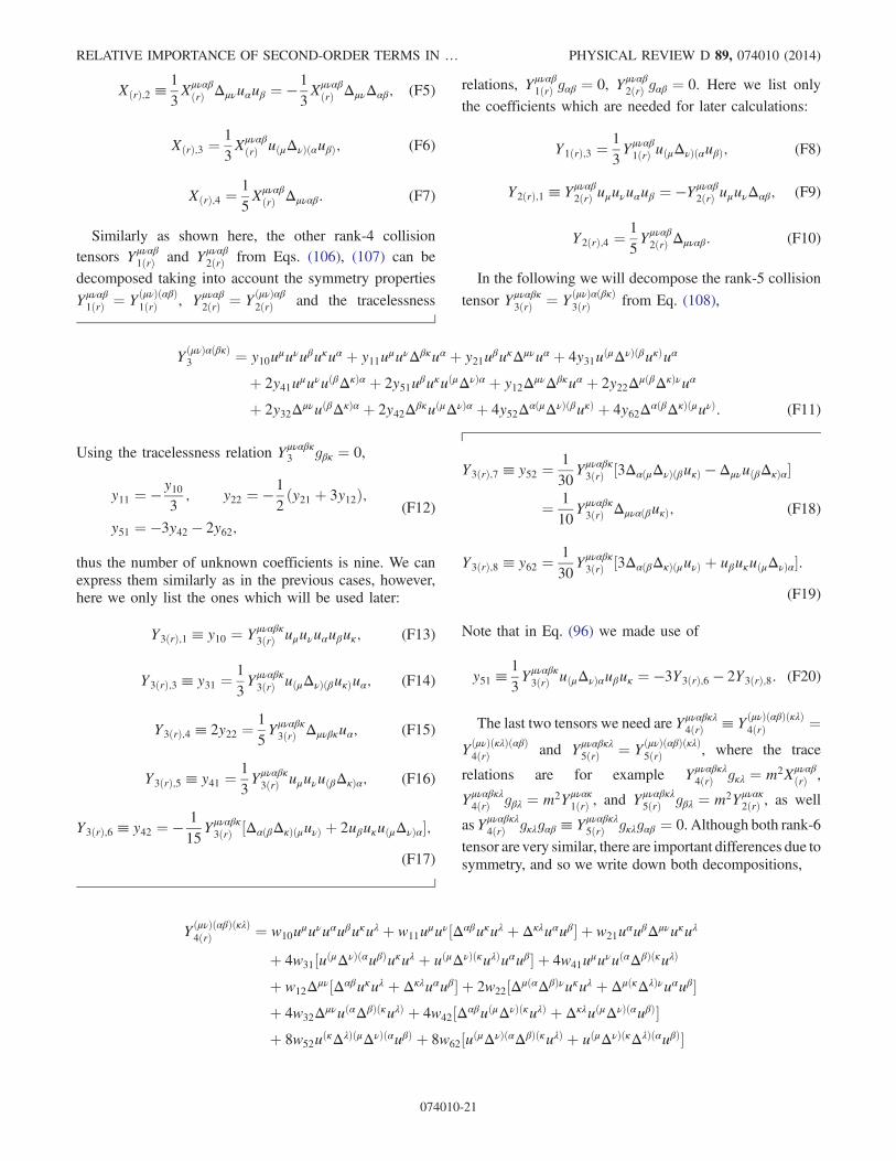
Similarly as shown here, the other rank-4 collisiontensors Yμναβ

1ðrÞ and Yμναβ2ðrÞ from Eqs. (106), (107) can be

decomposed taking into account the symmetry properties

Yμναβ1ðrÞ ¼ YðμνÞðαβÞ

1ðrÞ , Yμναβ2ðrÞ ¼ YðμνÞαβ

2ðrÞ and the tracelessness

relations, Yμναβ1ðrÞ gαβ ¼ 0, Yμναβ

2ðrÞ gαβ ¼ 0. Here we list only

the coefficients which are needed for later calculations:

Y1ðrÞ;3 ¼1

3Yμναβ1ðrÞ uðμΔνÞðαuβÞ; (F8)

Y2ðrÞ;1 ≡ Yμναβ2ðrÞ uμuνuαuβ ¼ −Yμναβ

2ðrÞ uμuνΔαβ; (F9)

Y2ðrÞ;4 ¼1

5Yμναβ2ðrÞ Δμναβ: (F10)

In the following we will decompose the rank-5 collision

tensor Yμναβκ3ðrÞ ¼ YðμνÞαðβκÞ

3ðrÞ from Eq. (108),

YðμνÞαðβκÞ3 ¼ y10uμuνuβuκuα þ y11uμuνΔβκuα þ y21uβuκΔμνuα þ 4y31uðμΔνÞðβuκÞuα

þ 2y41uμuνuðβΔκÞα þ 2y51uβuκuðμΔνÞα þ y12ΔμνΔβκuα þ 2y22ΔμðβΔκÞνuα

þ 2y32ΔμνuðβΔκÞα þ 2y42ΔβκuðμΔνÞα þ 4y52ΔαðμΔνÞðβuκÞ þ 4y62ΔαðβΔκÞðμuνÞ: (F11)

Using the tracelessness relation Yμναβκ3 gβκ ¼ 0,

y11 ¼ − y103

; y22 ¼ − 1

2ðy21 þ 3y12Þ;

y51 ¼ −3y42 − 2y62;(F12)

thus the number of unknown coefficients is nine. We canexpress them similarly as in the previous cases, however,here we only list the ones which will be used later:

Y3ðrÞ;1 ≡ y10 ¼ Yμναβκ3ðrÞ uμuνuαuβuκ; (F13)

Y3ðrÞ;3 ≡ y31 ¼1

3Yμναβκ3ðrÞ uðμΔνÞðβuκÞuα; (F14)

Y3ðrÞ;4 ≡ 2y22 ¼1

5Yμναβκ3ðrÞ Δμνβκuα; (F15)

Y3ðrÞ;5 ≡ y41 ¼1

3Yμναβκ3ðrÞ uμuνuðβΔκÞα; (F16)

Y3ðrÞ;6 ≡ y42 ¼ − 1

15Yμναβκ3ðrÞ ½ΔαðβΔκÞðμuνÞ þ 2uβuκuðμΔνÞα�;

(F17)

Y3ðrÞ;7 ≡ y52 ¼1

30Yμναβκ3ðrÞ ½3ΔαðμΔνÞðβuκÞ − ΔμνuðβΔκÞα�

¼ 1

10Yμναβκ3ðrÞ ΔμναðβuκÞ; (F18)

Y3ðrÞ;8 ≡ y62 ¼1

30Yμναβκ3ðrÞ ½3ΔαðβΔκÞðμuνÞ þ uβuκuðμΔνÞα�:

(F19)

Note that in Eq. (96) we made use of

y51 ≡ 1

3Yμναβκ3ðrÞ uðμΔνÞαuβuκ ¼ −3Y3ðrÞ;6 − 2Y3ðrÞ;8: (F20)

The last two tensors we need are Yμναβκλ4ðrÞ ≡ YðμνÞðαβÞðκλÞ

4ðrÞ ¼YðμνÞðκλÞðαβÞ4ðrÞ and Yμναβκλ

5ðrÞ ¼ YðμνÞðαβÞðκλÞ5ðrÞ , where the trace

relations are for example Yμναβκλ4ðrÞ gκλ ¼ m2Xμναβ

ðrÞ ,

Yμναβκλ4ðrÞ gβλ ¼ m2Yμνακ

1ðrÞ , and Yμναβκλ5ðrÞ gβλ ¼ m2Yμνακ

2ðrÞ , as well

as Yμναβκλ4ðrÞ gκλgαβ ≡ Yμναβκλ

5ðrÞ gκλgαβ ¼ 0. Although both rank-6

tensor are very similar, there are important differences due tosymmetry, and so we write down both decompositions,

YðμνÞðαβÞðκλÞ4ðrÞ ¼ w10uμuνuαuβuκuλ þ w11uμuν½Δαβuκuλ þ Δκλuαuβ� þ w21uαuβΔμνuκuλ

þ 4w31½uðμΔνÞðαuβÞuκuλ þ uðμΔνÞðκuλÞuαuβ� þ 4w41uμuνuðαΔβÞðκuλÞ

þ w12Δμν½Δαβuκuλ þ Δκλuαuβ� þ 2w22½ΔμðαΔβÞνuκuλ þ ΔμðκΔλÞνuαuβ�þ 4w32ΔμνuðαΔβÞðκuλÞ þ 4w42½ΔαβuðμΔνÞðκuλÞ þ ΔκλuðμΔνÞðαuβÞ�þ 8w52uðκΔλÞðμΔνÞðαuβÞ þ 8w62½uðμΔνÞðαΔβÞðκuλÞ þ uðμΔνÞðκΔλÞðαuβÞ�


074010-21

þ 2w72uμuνΔκðαΔβÞλ þ w82uμuνΔαβΔκλ þ w13ΔμνΔαβΔκλ þ 8w23ΔðκðμΔνÞðαΔβÞλÞ

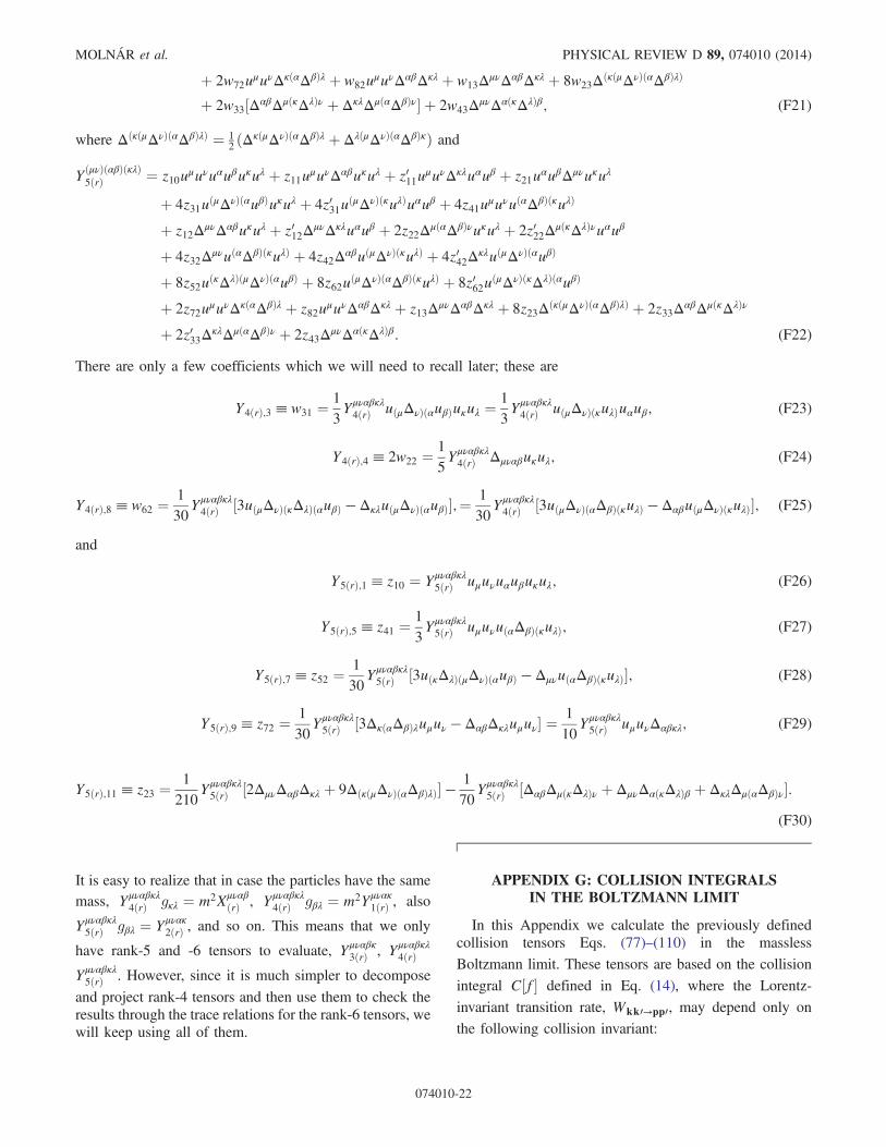
þ 2w33½ΔαβΔμðκΔλÞν þ ΔκλΔμðαΔβÞν� þ 2w43ΔμνΔαðκΔλÞβ; (F21)

where ΔðκðμΔνÞðαΔβÞλÞ ¼ 12ðΔκðμΔνÞðαΔβÞλ þ ΔλðμΔνÞðαΔβÞκÞ and

YðμνÞðαβÞðκλÞ5ðrÞ ¼ z10uμuνuαuβuκuλ þ z11uμuνΔαβuκuλ þ z011u

μuνΔκλuαuβ þ z21uαuβΔμνuκuλ

þ 4z31uðμΔνÞðαuβÞuκuλ þ 4z031uðμΔνÞðκuλÞuαuβ þ 4z41uμuνuðαΔβÞðκuλÞ

þ z12ΔμνΔαβuκuλ þ z012ΔμνΔκλuαuβ þ 2z22ΔμðαΔβÞνuκuλ þ 2z022ΔμðκΔλÞνuαuβ

þ 4z32ΔμνuðαΔβÞðκuλÞ þ 4z42ΔαβuðμΔνÞðκuλÞ þ 4z042ΔκλuðμΔνÞðαuβÞ

þ 8z52uðκΔλÞðμΔνÞðαuβÞ þ 8z62uðμΔνÞðαΔβÞðκuλÞ þ 8z062uðμΔνÞðκΔλÞðαuβÞ

þ 2z72uμuνΔκðαΔβÞλ þ z82uμuνΔαβΔκλ þ z13ΔμνΔαβΔκλ þ 8z23ΔðκðμΔνÞðαΔβÞλÞ þ 2z33ΔαβΔμðκΔλÞν

þ 2z033ΔκλΔμðαΔβÞν þ 2z43ΔμνΔαðκΔλÞβ: (F22)

There are only a few coefficients which we will need to recall later; these are

Y4ðrÞ;3 ≡ w31 ¼1

3Yμναβκλ4ðrÞ uðμΔνÞðαuβÞuκuλ ¼

1

3Yμναβκλ4ðrÞ uðμΔνÞðκuλÞuαuβ; (F23)

Y4ðrÞ;4 ≡ 2w22 ¼1

5Yμναβκλ4ðrÞ Δμναβuκuλ; (F24)

Y4ðrÞ;8 ≡ w62 ¼1

30Yμναβκλ4ðrÞ ½3uðμΔνÞðκΔλÞðαuβÞ − ΔκλuðμΔνÞðαuβÞ�;¼

1

30Yμναβκλ4ðrÞ ½3uðμΔνÞðαΔβÞðκuλÞ − ΔαβuðμΔνÞðκuλÞ�; (F25)

and

Y5ðrÞ;1 ≡ z10 ¼ Yμναβκλ5ðrÞ uμuνuαuβuκuλ; (F26)

Y5ðrÞ;5 ≡ z41 ¼1

3Yμναβκλ5ðrÞ uμuνuðαΔβÞðκuλÞ; (F27)

Y5ðrÞ;7 ≡ z52 ¼1

30Yμναβκλ5ðrÞ ½3uðκΔλÞðμΔνÞðαuβÞ − ΔμνuðαΔβÞðκuλÞ�; (F28)

Y5ðrÞ;9 ≡ z72 ¼1

30Yμναβκλ5ðrÞ ½3ΔκðαΔβÞλuμuν − ΔαβΔκλuμuν� ¼

1

10Yμναβκλ5ðrÞ uμuνΔαβκλ; (F29)

Y5ðrÞ;11 ≡ z23 ¼1

210Yμναβκλ5ðrÞ ½2ΔμνΔαβΔκλ þ 9ΔðκðμΔνÞðαΔβÞλÞ� − 1

70Yμναβκλ5ðrÞ ½ΔαβΔμðκΔλÞν þ ΔμνΔαðκΔλÞβ þ ΔκλΔμðαΔβÞν�:

(F30)

It is easy to realize that in case the particles have the samemass, Yμναβκλ

4ðrÞ gκλ ¼ m2XμναβðrÞ , Yμναβκλ

4ðrÞ gβλ ¼ m2Yμνακ1ðrÞ , also

Yμναβκλ5ðrÞ gβλ ¼ Yμνακ

2ðrÞ , and so on. This means that we only

have rank-5 and -6 tensors to evaluate, Yμναβκ3ðrÞ , Yμναβκλ

4ðrÞYμναβκλ5ðrÞ . However, since it is much simpler to decompose

and project rank-4 tensors and then use them to check theresults through the trace relations for the rank-6 tensors, wewill keep using all of them.

APPENDIX G: COLLISION INTEGRALSIN THE BOLTZMANN LIMIT

In this Appendix we calculate the previously definedcollision tensors Eqs. (77)–(110) in the massless

Boltzmann limit. These tensors are based on the collision

integral C½f� defined in Eq. (14), where the Lorentz-

invariant transition rate, Wkk0→pp0, may depend only on

the following collision invariant:


074010-22

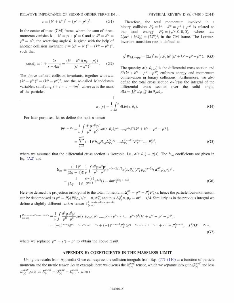
s≡ ðkμ þ k0μÞ2 ¼ ðpμ þ p0μÞ2: (G1)

In the center of mass (CM) frame, where the sum of three-momenta vanishes kþ k0 ¼ pþ p0 ¼ 0 and so k0 ¼ k00 ¼p0 ¼ p00, the scattering angle θs is given with the help ofanother collision invariant, t≡ ðkμ − pμÞ2 ¼ ðk0μ − p0μÞ2,such that

cos θs ≡ 1þ 2ts − 4m2

¼ ðkμ − k0μÞðpμ − p0μÞ

ðkμ − k0μÞ2 : (G2)

The above defined collision invariants, together with u≡ðkμ − p0μÞ2 ¼ ðk0μ − pμÞ2, are the so-called Mandelstamvariables, satisfying sþ tþ u ¼ 4m2, where m is the massof the particles.

Therefore, the total momentum involved in abinary collision Pμ

T ≡ kμ þ k0μ ¼ pμ þ p0μ is related tothe total energy Pμ

T ¼ ð ffiffiffis

p; 0; 0; 0Þ, where s≡

2ðm2 þ kμk0μÞ ¼ ð2k0Þ2, in the CM frame. The Lorentz-invariant transition rate is defined as

g2Wkk0→pp0 ¼ ð2πÞ6sσðs;θsÞδ4ðkμþk0μ−pμ−p0μÞ: (G3)

The quantity σðs; θCMÞ is the differential cross section andδ4ðkμ þ k0μ − pμ − p0μÞ enforces energy and momentumconservation in binary collisions. Furthermore, we alsodefine the total cross section σTðsÞas the integral of thedifferential cross section over the solid angle,dΩ ¼ R 2π0 dφ

Rπ0 sin θsdθs,

σTðsÞ ¼1

ν

Zπ

0

dΩσðs; θsÞ: (G4)

For later purposes, let us define the rank-n tensor

Θμ1:::::μn ≡ 1

ν

Zd3pp0

d3p0

p00 sσðs; θsÞpμ1 :::::pμnδ4ðkμ þ k0μ − pμ − p0μÞ;

¼X½n=2�q¼0

ð−1ÞqbnqBnqΔðμ1μ2PT

:::::Δμ2q−1μ2qPT

Pμ2qþ1

T :::::PμnÞT ; (G5)

where we assumed that the differential cross section is isotropic, i.e., σðs; θsÞ ¼ σðsÞ. The bnq coefficients are given inEq. (A2) and

Bnq ≡ ð−1Þqð2qþ 1Þ!!

1

ν

Zd3pp0

d3p0

p00 s−ðn−2qÞ=2σðs; θsÞðPμTpμÞn−2qðΔαβ

PTpαpβÞq;

¼ 1

ð2qþ 1Þ!!σTðsÞ2nþ1

s1=2ðs − 4m2Þð2qþ1Þ=2: (G6)

Here we defined the projection orthogonal to the total momentum,ΔαβP ¼ gμν − Pμ

TPνT=s, hence the particle four-momentum

can be decomposed as pμ ¼ PμTðPα

TpαÞ=sþ pαΔμαPT

and thusΔαβPTpαpβ ¼ m2 − s=4. Similarly as in the previous integral we

define a slightly different rank-n tensor Γμ1:::::μn−mνn−mþ1:::::νnðn;mÞ

Γμ1:::::μn−mνn−mþ1:::::νnðn;mÞ ≡ 1

ν

Zd3pp0

d3p0

p00 sσðs; θCMÞpμ1 :::::pμn−mp0νn−mþ1 :::::p0νnδ4ðkμ þ k0μ − pμ − p0μÞ;

¼ ð−1Þn−mΘμ1:::::μn−mνn−mþ1:::::νn þ ð−1Þn−m−1PνnT Θμ1:::::μn−mνn−mþ1:::::νn−1 þ � � � þ Pνn−mþ1

T :::::PνnT Θμ1:::::μn−m;

(G7)

where we replaced p0ν ¼ PνT − pν to obtain the above result.

APPENDIX H: COEFFICIENTS IN THE MASSLESS LIMIT

Using the results from Appendix G we can express the collision integrals from Eqs. (77)–(110) as a function of particlemomenta and the metric tensor. As an example, here we discuss the Xμναβ

ðrÞ tensor, which we separate into gain GμναβðrÞ and loss

LμναβðrÞ parts as Xμναβ

ðrÞ ¼ GμναβðrÞ − Lμναβ

ðrÞ , where


074010-23

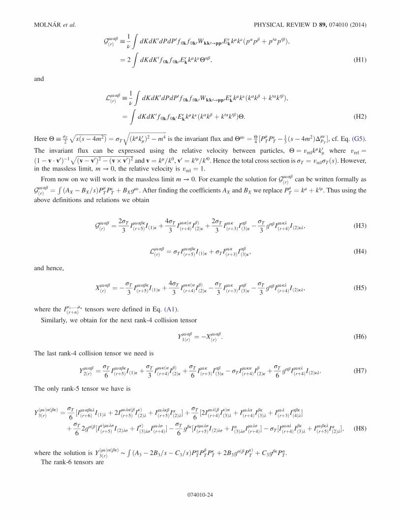
GμναβðrÞ ≡ 1

ν

ZdKdK0dPdP0f0kf0k0Wkk0→pp0Er

kkμkνðpαpβ þ p0αp0βÞ;

¼ 2

ZdKdK0f0kf0k0Er

kkμkνΘαβ; (H1)

and

LμναβðrÞ ≡ 1

ν

ZdKdK0dPdP0f0kf0k0Wkk0→pp0Er

kkμkνðkαkβ þ k0αk0βÞ;

¼Z

dKdK0f0kf0k0Erkk

μkνðkαkβ þ k0αk0βÞΘ: (H2)

Here Θ≡ σT2

ffiffiffiffiffiffiffiffiffiffiffiffiffiffiffiffiffiffiffiffiffiffisðs − 4m2Þ

p¼ σT

ffiffiffiffiffiffiffiffiffiffiffiffiffiffiffiffiffiffiffiffiffiffiffiffiffiffiðkμk0μÞ2 −m4

qis the invariant flux and Θμν ¼ Θ

4½Pμ

TPνT − 1

3ðs − 4m2ÞΔμν

PT�, cf. Eq. (G5).

The invariant flux can be expressed using the relative velocity between particles, Θ ¼ vrelkμk0μ where vrel ¼ð1 − v · v0Þ−1

ffiffiffiffiffiffiffiffiffiffiffiffiffiffiffiffiffiffiffiffiffiffiffiffiffiffiffiffiffiffiffiffiffiffiffiffiffiffiffiffiðv − v0Þ2 − ðv × v0Þ2

pand v ¼ kμ=k0, v0 ¼ k0μ=k00. Hence the total cross section is σT ¼ vrelσTðsÞ. However,

in the massless limit, m → 0, the relative velocity is vrel ¼ 1.

From now on we will work in the massless limit m → 0. For example the solution for GμναβðrÞ can be written formally as

GμναβðrÞ ¼ R ðAX − BX=sÞPμ

TPνT þ BXgμν. After finding the coefficients AX and BX we replace Pμ

T ¼ kμ þ k0μ. Thus using theabove definitions and relations we obtain

GμναβðrÞ ¼ 2σT

3Iμναβκðrþ5ÞIð1Þκ þ

4σT3

Iμνκðαðrþ4ÞIβÞð2Þκ þ

2σT3

Iμνκðrþ3ÞIαβð3Þκ −

σT3gαβIμνκλðrþ4ÞIð2Þκλ; (H3)

LμναβðrÞ ¼ σTI

μναβκðrþ5ÞIð1Þκ þ σTI

μνκðrþ3ÞI

αβð3Þκ; (H4)

and hence,

XμναβðrÞ ¼ − σT


4σT3

Iμνκðαðrþ4ÞIβÞð2Þκ −

σT3Iμνκðrþ3ÞI

αβð3Þκ −

σT3gαβIμνκλðrþ4ÞIð2Þκλ; (H5)

where the Iμ1:::::μnðrþnÞ tensors were defined in Eq. (A1).

Similarly, we obtain for the next rank-4 collision tensor

Yμναβ1ðrÞ ¼ −Xμναβ

ðrÞ : (H6)

The last rank-4 collision tensor we need is

Yμναβ2ðrÞ ¼ σT


σT3Iμνκðαðrþ4ÞI

βÞð2Þκ þ

σT6Iμνκðrþ3ÞI

αβð3Þκ − σTI

μνκαðrþ4ÞI

βð2Þκ þ

σT6gαβIμνκλðrþ4ÞIð2Þκλ: (H7)

The only rank-5 tensor we have is

YðμνÞαðβκÞ3ðrÞ ¼ σT

6½Iμναβκλðrþ6Þ Ið1Þλ þ 2Iμνλαðβðrþ5Þ I

κÞð2Þλ þ Iμνλκβðrþ5ÞI

αð2Þλ� þ

σT6½2Iμνλðβðrþ4ÞI

κÞαð3Þλ þ Iμνλαðrþ4ÞI

βκð3Þλ þ Iμνλðrþ3ÞI

αβκð4Þλ�

þ σT62gαðβ½IκÞμνλσðrþ5Þ Ið2Þλσ þ IκÞð3ÞλσI

μνλσðrþ4Þ� −

σT6gβκ½Iαμνλσðrþ5ÞIð2Þλσ þ Iαð3ÞλσI

μνλσðrþ4Þ� − σT ½Iμναλðrþ4ÞI

βκð3Þλ þ Iμνβκλðrþ5ÞI

αð2Þλ�; (H8)

where the solution is YðμνÞαðβκÞ3ðrÞ ∼

R ðA3 − 2B3=s − C3=sÞPαTP

βTP

κT þ 2B3gαðβP

κÞT þ C3gβκPα

T .The rank-6 tensors are


074010-24

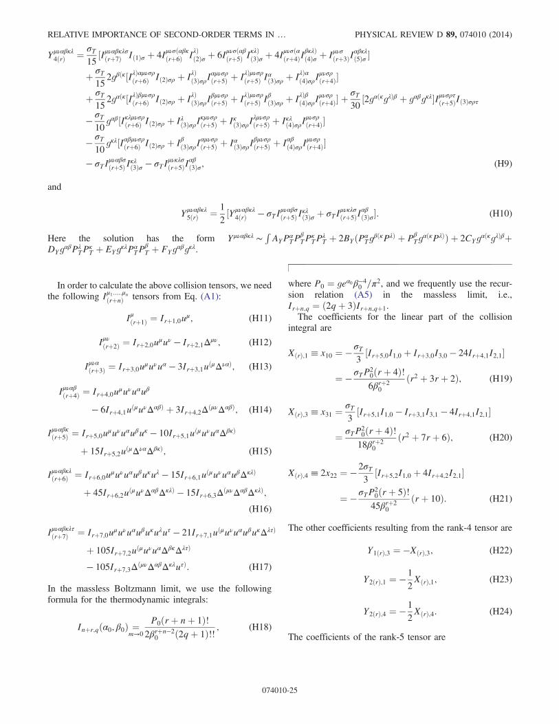
Yμναβκλ4ðrÞ ¼ σT

15½Iμναβκλσðrþ7Þ Ið1Þσ þ 4Iμνσðαβκðrþ6Þ IλÞð2Þσ þ 6Iμνσðαβðrþ5Þ I

κλÞð3Þσ þ 4Iμνσðαðrþ4ÞI

βκλÞð4Þσ þ Iμνσðrþ3ÞI

αβκλð5Þσ �

þ σT15

2gβðκ½IλÞαμνσρðrþ6Þ Ið2Þσρ þ IλÞð3ÞσρIαμνσρðrþ5Þ þ IλÞμνσρðrþ5Þ I

αð3Þσρ þ IλÞαð4ÞσρI

μνσρðrþ4Þ�

þ σT15

2gαðκ½IλÞβμνσρðrþ6Þ Ið2Þσρ þ IλÞð3ÞσρIβμνσρðrþ5Þ þ IλÞμνσρðrþ5Þ I

βð3Þσρ þ IλÞβð4ÞσρI

μνσρðrþ4Þ� þ

σT30

½2gαðκgλÞβ þ gαβgκλ�Iμνσρτðrþ5ÞIð3Þσρτ

− σT10

gαβ½Iκλμνσρðrþ6Þ Ið2Þσρ þ Iλð3ÞσρIκμνσρðrþ5Þ þ Iκð3ÞσρI

λμνσρðrþ5Þ þ Iκλð4ÞσρI

μνσρðrþ4Þ�

− σT10

gκλ½Iαβμνσρðrþ6Þ Ið2Þσρ þ Iβð3ÞσρIαμνσρðrþ5Þ þ Iαð3ÞσρI

βμνσρðrþ5Þ þ Iαβð4ÞσρI

μνσρðrþ4Þ�

− σTIμναβσðrþ5Þ I

κλð3Þσ − σTI

μνκλσðrþ5ÞI

αβð3Þσ; (H9)

and


2½Yμναβκλ

4ðrÞ − σTIμναβσðrþ5Þ I

κλð3Þσ þ σTI

μνκλσðrþ5ÞI

αβð3Þσ�: (H10)

Here the solution has the form Yμναβκλ ∼RAYPα

TPβTP

κTP

λT þ 2BYðPα

TgβðκPλÞ þ Pβ

TgαðκPλÞÞ þ 2CYgαðκgλÞβþ

DYgαβPλTP

κT þ EYgκλPα

TPβT þ FYgαβgκλ.

In order to calculate the above collision tensors, we needthe following Iμ1:::::μnðrþnÞ tensors from Eq. (A1):

Iμðrþ1Þ ¼ Irþ1;0uμ; (H11)

Iμνðrþ2Þ ¼ Irþ2;0uμuν − Irþ2;1Δμν; (H12)

Iμναðrþ3Þ ¼ Irþ3;0uμuνuα − 3Irþ3;1uðμΔναÞ; (H13)

Iμναβðrþ4Þ ¼ Irþ4;0uμuνuαuβ

− 6Irþ4;1uðμuνΔαβÞ þ 3Irþ4;2ΔðμνΔαβÞ; (H14)

Iμναβκðrþ5Þ ¼ Irþ5;0uμuνuαuβuκ − 10Irþ5;1uðμuνuαΔβκÞ

þ 15Irþ5;2uðμΔναΔβκÞ; (H15)

Iμναβκλðrþ6Þ ¼ Irþ6;0uμuνuαuβuκuλ − 15Irþ6;1uðμuνuαuβΔκλÞ

þ 45Irþ6;2uðμuνΔαβΔκλÞ − 15Irþ6;3ΔðμνΔαβΔκλÞ;

(H16)

Iμναβκλτðrþ7Þ ¼ Irþ7;0uμuνuαuβuκuλuτ − 21Irþ7;1uðμuνuαuβuκΔλτÞ

þ 105Irþ7;2uðμuνuαΔβκΔλτÞ

− 105Irþ7;3ΔðμνΔαβΔκλuτÞ: (H17)

In the massless Boltzmann limit, we use the followingformula for the thermodynamic integrals:

Inþr;qðα0; β0Þ ¼m→0

P0ðrþ nþ 1Þ!2βrþn−2

0 ð2qþ 1Þ!! ; (H18)

where P0 ¼ geα0β−40 =π2, and we frequently use the recur-sion relation (A5) in the massless limit, i.e.,Irþn;q ¼ ð2qþ 3ÞIrþn;qþ1.The coefficients for the linear part of the collision

integral are

XðrÞ;1 ≡ x10 ¼ − σT3½Irþ5;0I1;0 þ Irþ3;0I3;0 − 24Irþ4;1I2;1�

¼ − σTP20ðrþ 4Þ!6βrþ2

0

ðr2 þ 3rþ 2Þ; (H19)

XðrÞ;3 ≡ x31 ¼σT3½Irþ5;1I1;0 − Irþ3;1I3;1 − 4Irþ4;1I2;1�

¼ σTP20ðrþ 4Þ!18βrþ2

0

ðr2 þ 7rþ 6Þ; (H20)

XðrÞ;4 ≡ 2x22 ¼ − 2σT3

½Irþ5;2I1;0 þ 4Irþ4;2I2;1�


0

ðrþ 10Þ: (H21)

The other coefficients resulting from the rank-4 tensor are

Y1ðrÞ;3 ¼ −XðrÞ;3; (H22)

Y2ðrÞ;1 ¼ − 1

2XðrÞ;1; (H23)

Y2ðrÞ;4 ¼ − 1

2XðrÞ;4: (H24)

The coefficients of the rank-5 tensor are


074010-25

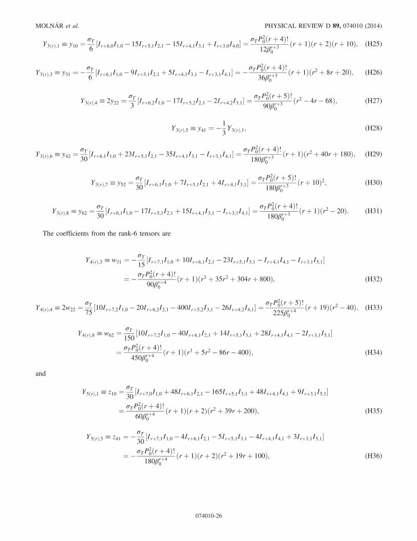
Y3ðrÞ;1 ≡ y10 ¼σT6½Irþ6;0I1;0 − 15Irþ5;1I2;1 − 15Irþ4;1I3;1 þ Irþ3;0I4;0� ¼

σTP20ðrþ 4Þ!12βrþ3

0

ðrþ 1Þðrþ 2Þðrþ 10Þ; (H25)

Y3ðrÞ;3 ≡ y31 ¼ − σT6½Irþ6;1I1;0 − 9Irþ5;1I2;1 þ 5Irþ4;1I3;1 − Irþ3;1I4;1� ¼ − σTP2

0ðrþ 4Þ!36βrþ3

0

ðrþ 1Þðr2 þ 8rþ 20Þ; (H26)

Y3ðrÞ;4 ≡ 2y22 ¼σT3½Irþ6;2I1;0 − 17Irþ5;2I2;1 − 2Irþ4;2I3;1� ¼

σTP20ðrþ 5Þ!90βrþ3

0

ðr2 − 4r − 68Þ; (H27)

Y3ðrÞ;5 ≡ y41 ¼ − 1

3Y3ðrÞ;1; (H28)

Y3ðrÞ;6 ≡ y42 ¼σT30

½Irþ6;1I1;0 þ 23Irþ5;1I2;1 − 35Irþ4;1I3;1 − Irþ3;1I4;1� ¼σTP2

0ðrþ 4Þ!180βrþ3

0

ðrþ 1Þðr2 þ 40rþ 180Þ; (H29)

Y3ðrÞ;7 ≡ y52 ¼σT30

½Irþ6;1I1;0 þ 7Irþ5;1I2;1 þ 4Irþ4;1I3;1� ¼σTP2


0

ðrþ 10Þ2; (H30)

Y3ðrÞ;8 ≡ y62 ¼σT30

½Irþ6;1I1;0 − 17Irþ5;1I2;1 þ 15Irþ4;1I3;1 − Irþ3;1I4;1� ¼σTP2


0

ðrþ 1Þðr2 − 20Þ: (H31)

The coefficients from the rank-6 tensors are

Y4ðrÞ;3 ≡ w31 ¼ − σT15

½Irþ7;1I1;0 þ 10Irþ6;1I2;1 − 23Irþ5;1I3;1 − Irþ4;1I4;1 − Irþ3;1I5;1�


0

ðrþ 1Þðr3 þ 35r2 þ 304rþ 800Þ; (H32)

Y4ðrÞ;4 ≡ 2w22 ¼σT75

½10Irþ7;2I1;0 − 20Irþ6;2I2;1 − 400Irþ5;2I3;1 − 26Irþ4;2I4;1� ¼σTP2


0

ðrþ 19Þðr2 − 40Þ; (H33)

Y4ðrÞ;8 ≡ w62 ¼σT150

½10Irþ7;2I1;0 − 40Irþ6;1I2;1 þ 14Irþ5;1I3;1 þ 28Irþ4;1I4;1 − 2Irþ3;1I5;1�

¼ σTP20ðrþ 4Þ!

450βrþ40

ðrþ 1Þðr3 þ 5r2 − 86r − 400Þ; (H34)

and

Y5ðrÞ;1 ≡ z10 ¼σT30

½Irþ7;0I1;0 þ 48Irþ6;1I2;1 − 165Irþ5;1I3;1 þ 48Irþ4;1I4;1 þ 9Irþ3;1I5;1�

¼ σTP20ðrþ 4Þ!60βrþ4

0

ðrþ 1Þðrþ 2Þðr2 þ 39rþ 200Þ; (H35)

Y5ðrÞ;5 ≡ z41 ¼ − σT30

½Irþ7;1I1;0 − 4Irþ6;1I2;1 − 5Irþ5;1I3;1 − 4Irþ4;1I4;1 þ 3Irþ3;1I5;1�

¼ − σTP20ðrþ 4Þ!

180βrþ40

ðrþ 1Þðrþ 2Þðr2 þ 19rþ 100Þ; (H36)


074010-26

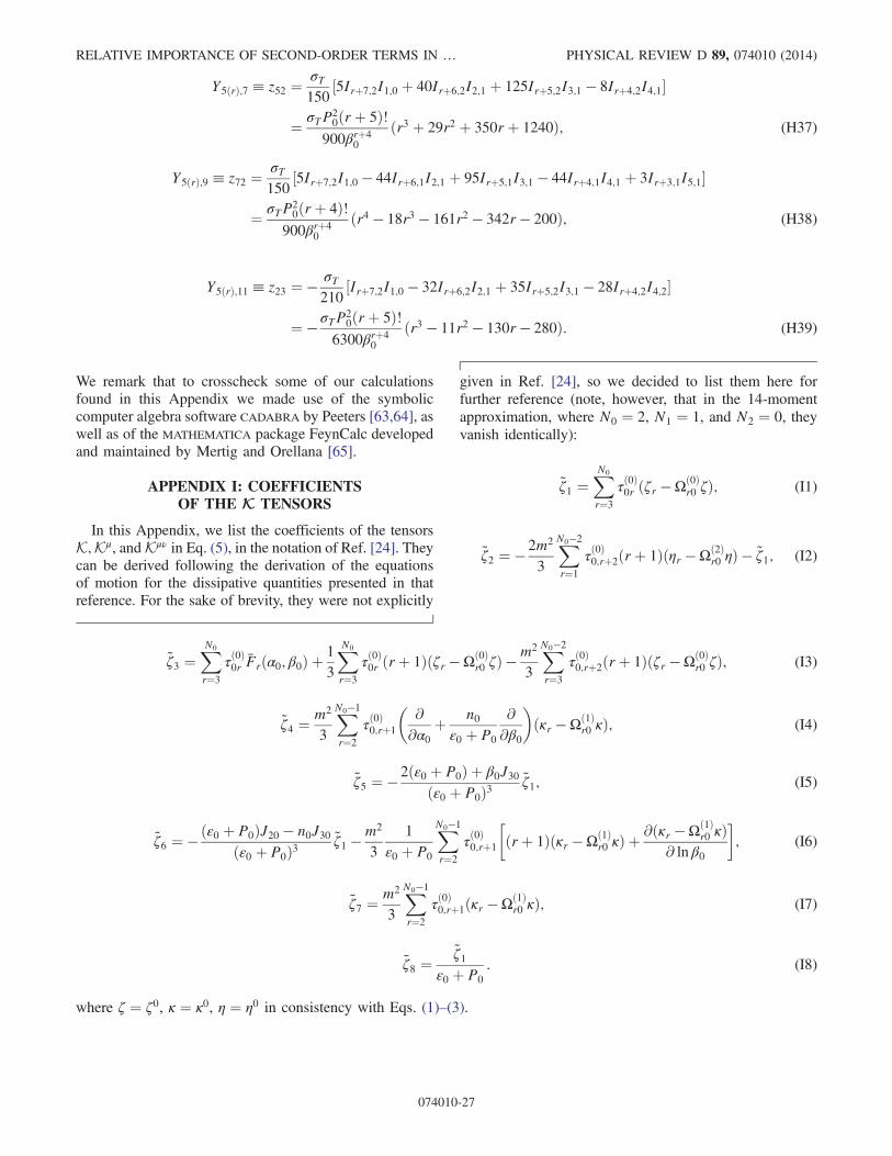
Y5ðrÞ;7 ≡ z52 ¼σT150

½5Irþ7;2I1;0 þ 40Irþ6;2I2;1 þ 125Irþ5;2I3;1 − 8Irþ4;2I4;1�

¼ σTP20ðrþ 5Þ!

900βrþ40

ðr3 þ 29r2 þ 350rþ 1240Þ; (H37)

Y5ðrÞ;9 ≡ z72 ¼σT150

½5Irþ7;2I1;0 − 44Irþ6;1I2;1 þ 95Irþ5;1I3;1 − 44Irþ4;1I4;1 þ 3Irþ3;1I5;1�

¼ σTP20ðrþ 4Þ!

900βrþ40

ðr4 − 18r3 − 161r2 − 342r − 200Þ; (H38)

Y5ðrÞ;11 ≡ z23 ¼ − σT210

½Irþ7;2I1;0 − 32Irþ6;2I2;1 þ 35Irþ5;2I3;1 − 28Irþ4;2I4;2�

¼ − σTP20ðrþ 5Þ!

6300βrþ40

ðr3 − 11r2 − 130r − 280Þ: (H39)

We remark that to crosscheck some of our calculationsfound in this Appendix we made use of the symboliccomputer algebra software CADABRA by Peeters [63,64], aswell as of the MATHEMATICA package FeynCalc developedand maintained by Mertig and Orellana [65].

APPENDIX I: COEFFICIENTSOF THE K TENSORS

In this Appendix, we list the coefficients of the tensorsK;Kμ, andKμν in Eq. (5), in the notation of Ref. [24]. Theycan be derived following the derivation of the equationsof motion for the dissipative quantities presented in thatreference. For the sake of brevity, they were not explicitly

given in Ref. [24], so we decided to list them here forfurther reference (note, however, that in the 14-momentapproximation, where N0 ¼ 2, N1 ¼ 1, and N2 ¼ 0, theyvanish identically):

~ζ1 ¼XN0

r¼3

τð0Þ0r ðζr −Ωð0Þr0 ζÞ; (I1)

~ζ2 ¼ − 2m2

3

XN0−2

r¼1

τð0Þ0;rþ2ðrþ 1Þðηr −Ωð2Þr0 ηÞ − ~ζ1; (I2)

~ζ3 ¼XN0

r¼3

τð0Þ0r Frðα0; β0Þ þ1

3

XN0

r¼3

τð0Þ0r ðrþ 1Þðζr −Ωð0Þr0 ζÞ −m2

3

XN0−2

r¼3

τð0Þ0;rþ2ðrþ 1Þðζr −Ωð0Þr0 ζÞ; (I3)

~ζ4 ¼m2

3

XN0−1

r¼2

τð0Þ0;rþ1

� ∂∂α0 þ

n0ε0 þ P0

∂∂β0�ðκr −Ωð1Þ

r0 κÞ; (I4)

~ζ5 ¼ − 2ðε0 þ P0Þ þ β0J30ðε0 þ P0Þ3

~ζ1; (I5)

~ζ6 ¼ − ðε0 þ P0ÞJ20 − n0J30ðε0 þ P0Þ3

~ζ1 −m2

3

1

ε0 þ P0

XN0−1

r¼2

τð0Þ0;rþ1

�ðrþ 1Þðκr −Ωð1Þ

r0 κÞ þ∂ðκr −Ωð1Þ

r0 κÞ∂ ln β0

�; (I6)

~ζ7 ¼m2

3

XN0−1

r¼2

τð0Þ0;rþ1ðκr −Ωð1Þr0 κÞ; (I7)

~ζ8 ¼~ζ1

ε0 þ P0

: (I8)

where ζ ¼ ζ0, κ ¼ κ0, η ¼ η0 in consistency with Eqs. (1)–(3).


074010-27

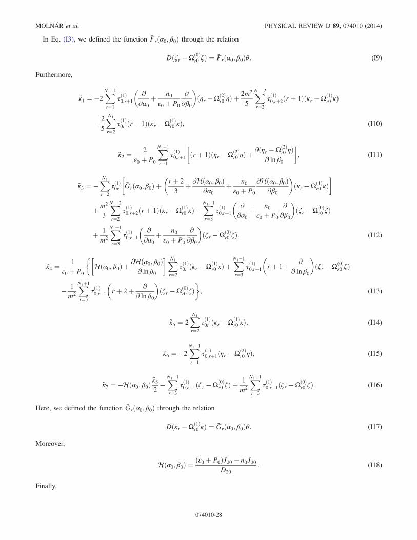
In Eq. (I3), we defined the function Frðα0; β0Þ through the relation

Dðζr −Ωð0Þr0 ζÞ ¼ Frðα0; β0Þθ: (I9)

Furthermore,

~κ1 ¼ −2XN1−1

r¼1

τð1Þ0;rþ1

� ∂∂α0 þ

n0ε0 þ P0

∂∂β0�ðηr −Ωð2Þ

r0 ηÞ þ2m2

5

XN1−2

r¼2

τð1Þ0;rþ2ðrþ 1Þðκr −Ωð1Þr0 κÞ

− 2

5

XN1

r¼2

τð1Þ0r ðr − 1Þðκr −Ωð1Þr0 κÞ; (I10)

~κ2 ¼2

ε0 þ P0

XN1−1

r¼1

τð1Þ0;rþ1

�ðrþ 1Þðηr −Ωð2Þ

r0 ηÞ þ∂ðηr −Ωð2Þ

r0 ηÞ∂ ln β0

�; (I11)

~κ3 ¼ −XN1

r¼2

τð1Þ0r

�Grðα0; β0Þ þ

�rþ 2

3þ ∂Hðα0; β0Þ

∂α0 þ n0ε0 þ P0

∂Hðα0; β0Þ∂β0

�ðκr −Ωð1Þ

r0 κÞ�

þm2

3

XN1−2

r¼2

τð1Þ0;rþ2ðrþ 1Þðκr −Ωð1Þr0 κÞ −

XN1−1

r¼3

τð1Þ0;rþ1

� ∂∂α0 þ

n0ε0 þ P0

∂∂β0�ðζr −Ωð0Þ

r0 ζÞ

þ 1

m2

XN1þ1

r¼3

τð1Þ0;r−1� ∂∂α0 þ

n0ε0 þ P0

∂∂β0�ðζr −Ωð0Þ

r0 ζÞ; (I12)

~κ4 ¼1

ε0 þ P0

��Hðα0; β0Þ þ

∂Hðα0; β0Þ∂ ln β0

�XN1

r¼2

τð1Þ0r ðκr −Ωð1Þr0 κÞ þ

XN1−1

r¼3

τð1Þ0;rþ1

�rþ 1þ ∂

∂ ln β0�ðζr −Ωð0Þ

r0 ζÞ

− 1

m2

XN1þ1

r¼3

τð1Þ0;r−1�rþ 2þ ∂

∂ ln β0�ðζr −Ωð0Þ

r0 ζÞ�; (I13)

~κ5 ¼ 2XN1

r¼2

τð1Þ0r ðκr −Ωð1Þr0 κÞ; (I14)

~κ6 ¼ −2XN1−1

r¼1

τð1Þ0;rþ1ðηr −Ωð2Þr0 ηÞ; (I15)

~κ7 ¼ −Hðα0; β0Þ~κ52− XN1−1

r¼3

τð1Þ0;rþ1ðζr −Ωð0Þr0 ζÞ þ

1

m2

XN1þ1

r¼3

τð1Þ0;r−1ðζr −Ωð0Þr0 ζÞ: (I16)

Here, we defined the function Grðα0; β0Þ through the relation

Dðκr −Ωð1Þr0 κÞ ¼ Grðα0; β0Þθ: (I17)

Moreover,

Hðα0; β0Þ ¼ðε0 þ P0ÞJ20 − n0J30

D20

: (I18)

Finally,


074010-28

~η1 ¼ 2XN2

r¼1

τð2Þ0r ðηr −Ωð2Þr0 ηÞ; (I19)

~η2 ¼ 2

�−XN2

r¼1

τð2Þ0r

�Hrðα0; β0Þ þ

1

3ðrþ 2Þðηr −Ωð2Þ

r0 ηÞ�

þm2

3

XN2−2

r−1τð2Þ0;rþ2ðrþ 1Þðηr −Ωð2Þ

r0 ηÞ þm2

5

XN2−2

r¼3

τð2Þ0;rþ2ðrþ 1Þðζr −Ωð0Þr0 ζÞ

− 1

5

XN2

r¼3

τð2Þ0r ð2rþ 3Þðζr −Ωð0Þr0 ζÞ þ

1

5m2

XN2þ2

r¼3

τð2Þ0;r−2ðrþ 2Þðζr −Ωð0Þr0 ζÞ

�; (I20)

~η3 ¼2

7

�−XN2

r¼1

τð2Þ0r ð4rþ 3Þðηr −Ωð2Þr0 ηÞ þ 4m2

XN2−2

r¼1

τð2Þ0;rþ2ðrþ 1Þðηr −Ωð2Þr0 ηÞ

�; (I21)

~η4 ¼ 2~η1; (I22)

~η5 ¼2

5

�XN2þ1

r¼2

τð2Þ0;r−1� ∂∂α0 þ

n0ε0 þ P0


r0 κÞ −m2XN2−1

r¼2

τð2Þ0;rþ1

� ∂∂α0 þ

n0ε0 þ P0


r0 κÞ�; (I23)

~η6 ¼2ðε0 þ P0Þ þ β0J30

ðε0 þ P0Þ3~η1; (I24)

~η7 ¼2

5ðε0 þ P0Þ�5

2

ðε0 þ P0ÞJ20 − n0J30ðε0 þ P0Þ2

~η1 −XN2þ1

r¼2

τð2Þ0;r−1�rþ 4þ ∂

∂ ln β0�ðκr −Ωð1Þ

r0 κÞ

þm2XN2−1

r¼2

τð2Þ0;rþ1

�rþ 1þ ∂

∂ ln β0�ðκr −Ωð1Þ

r0 κÞ�; (I25)

~η8 ¼2

5

�XN2þ1

r¼2

τð2Þ0;r−1ðκr −Ωð1Þr0 κÞ −m2

XN2−1

r¼2

τð2Þ0;rþ1ðκr −Ωð1Þr0 κÞ

�; (I26)

~η9 ¼ − ~η1ε0 þ P0

: (I27)

Here, we defined the function Hrðα0; β0Þ through the relation

Dðηr −Ωð2Þr0 ηÞ ¼ Hrðα0; β0Þθ: (I28)

[1] U.W. Heinz and R. Snellings, Annu. Rev. Nucl. Part. Sci.63, 123 (2013).

[2] C. Gale, S. Jeon, and B. Schenke, Int. J. Mod. Phys. A 28,1340011 (2013).

[3] L. Baiotti, B. Giacomazzo, and L. Rezzolla, Phys. Rev. D78, 084033 (2008).

[4] N. Andersson and G. L. Comer, Living Rev. Relativity 10, 1(2007), http://www.livingreviews.org/lrr‑2007‑1.

[5] R. Maartens, arXiv:astro-ph/9609119.[6] R. Maartens, Classical Quantum Gravity 12, 1455 (1995).[7] W. Zimdahl, D. Pavon, and R. Maartens, Phys. Rev. D 55,

4681 (1997).[8] X. Chen and E. A. Spiegel, Classical Quantum Gravity 28,

175003 (2011).[9] P. Danielewicz and M. Gyulassy, Phys. Rev. D 31, 53

(1985).


074010-29

http://dx.doi.org/10.1146/annurev-nucl-102212-170540

http://dx.doi.org/10.1146/annurev-nucl-102212-170540

http://dx.doi.org/10.1142/S0217751X13400113

http://dx.doi.org/10.1142/S0217751X13400113



http://dx.doi.org/10.12942/lrr-2007-1


http://www.livingreviews.org/lrr-2007-1



http://arXiv.org/abs/astro-ph/9609119

http://dx.doi.org/10.1088/0264-9381/12/6/011



http://dx.doi.org/10.1088/0264-9381/28/17/175003

http://dx.doi.org/10.1088/0264-9381/28/17/175003



[10] P. Kovtun, D. T. Son, and A. O. Starinets, Phys. Rev. Lett.94, 111601 (2005).

[11] L. P. Csernai, J. I. Kapusta, and L. D. McLerran, Phys. Rev.Lett. 97, 152303 (2006).

[12] C. Eckart, Phys. Rev. 58, 919 (1940).[13] L. D. Landau and E. M. Lifshitz, Fluid Dynamics

(Butterworth-Heinemann Linacre House, Jordan Hill,Oxford, 1987), 2nd ed.

[14] W. A. Hiscock and L. Lindblom, Ann. Phys. (N.Y.) 151, 466(1983); Phys. Rev. D 31, 725 (1985); 353723 (1987); Phys.Lett. 131A, 509 (1988); 131A509 (1988).

[15] S. Pu, T. Koide, and D. H. Rischke, Phys. Rev. D 81, 114039(2010).

[16] H. Grad, Commun. Pure Appl. Math. 2, 331 (1949).[17] I. Müller, Z. Phys. 198, 329 (1967).[18] I.-S. Liu, I. Müller, and T. Ruggeri, Ann. Phys. (N.Y.) 169,

191 (1986).[19] I. Müller, Living Rev. Relativity 2, 1 (1999), http://www

.livingreviews.org/lrr‑1999‑1.[20] J. M. Stewart, Non-Equilibrium Relativistic Kinetic Theory,

Lecture Notes in Physics (Springer-Verlag, Berlin, 1971),Vol. 10.

[21] J. M. Stewart, Proc. R. Soc. A 357, 59 (1977); W. Israel andJ. M. Stewart, ibid. 365, 43 (1979).

[22] W. Israel and J. M. Stewart, Ann. Phys. (N.Y.) 118, 341(1979).

[23] G. S. Denicol, T. Koide, and D. H. Rischke, Phys. Rev. Lett.105, 162501 (2010).

[24] G. S. Denicol, H. Niemi, E. Molnar, and D. H. Rischke,Phys. Rev. D 85, 114047 (2012).

[25] G. S. Denicol, E. Molnar, H. Niemi, and D. H. Rischke, Eur.Phys. J. A 48, 170 (2012).

[26] B. Betz, D. Henkel, and D. H. Rischke, Prog. Part. Nucl.Phys. 62, 556 (2009); J. Phys. G 36, 064029 (2009).

[27] B. Betz, G. S. Denicol, T. Koide, E. Molnár, H. Niemi, andD. H. Rischke, EPJ Web Conf. 13, 07005 (2011).

[28] A. Muronga, Phys. Rev. C 76, 014909 (2007).[29] T. Tsumura, T. Kunihiro, and K. Ohnishi, Phys. Lett. B 646,

134 (2007).[30] K. Tsumura and T. Kunihiro, Phys. Lett. B 690, 255 (2010).[31] K. Tsumura and T. Kunihiro, Prog. Theor. Phys. Suppl. 195,

19 (2012).[32] M. A. York and G. D. Moore, Phys. Rev. D 79, 054011

(2009).[33] A. Monnai and T. Hirano, Phys. Rev. C 80, 054906

(2009).[34] A. Monnai and T. Hirano, Nucl. Phys. A847, 283 (2010).[35] W. Florkowski and R. Ryblewski, Phys. Rev. C 83, 034907

(2011).[36] M. Martinez and M. Strickland, Nucl. Phys. A848, 183

(2010).

[37] A. Jaiswal, R. S. Bhalerao, and S. Pal, Phys. Lett. B 720,347 (2013).

[38] A. Jaiswal, Phys. Rev. C 87, 051901 (2013).[39] A. Jaiswal, Phys. Rev. C 88, 021903 (2013).[40] D. Teaney and L. Yan, Phys. Rev. C 89, 014901 (2014).[41] D. Jou, J. Casas-Vázquez, and G. Lebon, Rep. Prog. Phys.

51, 1105 (1988).[42] D. Jou, J. Casas-Vázquez, and G. Lebon, Rep. Prog. Phys.

62, 1035 (1999).[43] J. Gariel and G. Le Denmat, Phys. Rev. D 50, 2560 (1994).[44] T. Koide, G. S. Denicol, P. Mota, and T. Kodama, Phys. Rev.

C 75, 034909 (2007).[45] A. El, Z. Xu, and C. Greiner, Phys. Rev. C 81, 041901

(2010).[46] P. Van and T. S. Biro, Eur. Phys. J. Spec. Top. 155, 201

(2008).[47] T. S. Biro, E. Molnar, and P. Van, Phys. Rev. C 78, 014909

(2008).[48] P. Van and T. S. Biro, Phys. Lett. B 709, 106 (2012).[49] A. Muronga, J. Phys. G 37, 094008 (2010).[50] T. Osada, Phys. Rev. C 85, 014906 (2012).[51] A. Jaiswal, R. S. Bhalerao, and S. Pal, Phys. Rev. C 87,

021901 (2013).[52] G. S. Denicol, J. Noronha, H. Niemi, and D. H. Rischke,

Phys. Rev. D 83, 074019 (2011).[53] G. S. Denicol, H. Niemi, I. Bouras, E. Molnar, Z. Xu, D. H.

Rischke, and C. Greiner, arXiv:1207.6811.[54] S. R. de Groot, W. A. van Leeuwen, and Ch. G. van Weert,

Relativistic Kinetic Theory—Principles and Applications(North-Holland, Amsterdam, 1980).

[55] C. Cercignani and G. M. Kremer, The RelativisticBoltzmann Equation: Theory and Applications (BirkhäuserVerlag, Basel-Boston-Berlin, 2002).

[56] J. L. Anderson, J. Math. Phys. (N.Y.) 15, 1116 (1974).[57] H. Struchtrup, Ann. Phys. (N.Y.) 257, 111 (1997).[58] H. Struchtrup, Phys. A (Amsterdam, Neth.) 253, 555

(1998).[59] P. Huovinen and D. Molnar, Phys. Rev. C 79, 014906

(2009).[60] I. Bouras, E. Molnar, H. Niemi, Z. Xu, A. El, O. Fochler,

C. Greiner, and D. H. Rischke, Nucl. Phys. A830, 741c(2009).

[61] I. Bouras, E. Molnar, H. Niemi, Z. Xu, A. El, O. Fochler,C. Greiner, and D. H. Rischke, Phys. Rev. C 82, 024910(2010).

[62] W. Florkowski, R. Ryblewski, and M. Strickland, Phys.Rev. C 88, 024903 (2013).

[63] K. Peeters, Comput. Phys. Commun. 176, 550 (2007).[64] K. Peeters, arXiv:hep-th/0701238.[65] R. Mertig, M. Bohm, and A. Denner, Comput. Phys.

Commun. 64, 345 (1991).


074010-30

http://dx.doi.org/10.1103/PhysRevLett.94.111601




http://dx.doi.org/10.1103/PhysRev.58.919

http://dx.doi.org/10.1016/0003-4916(83)90288-9

http://dx.doi.org/10.1016/0003-4916(83)90288-9



http://dx.doi.org/10.1016/0375-9601(88)90679-2

http://dx.doi.org/10.1016/0375-9601(88)90679-2

http://dx.doi.org/10.1016/0375-9601(88)90679-2



http://dx.doi.org/10.1002/cpa.3160020403

http://dx.doi.org/10.1007/BF01326412

http://dx.doi.org/10.1016/0003-4916(86)90164-8

http://dx.doi.org/10.1016/0003-4916(86)90164-8





http://dx.doi.org/10.1098/rspa.1977.0155

http://dx.doi.org/10.1098/rspa.1979.0005

http://dx.doi.org/10.1016/0003-4916(79)90130-1

http://dx.doi.org/10.1016/0003-4916(79)90130-1




http://dx.doi.org/10.1140/epja/i2012-12170-x

http://dx.doi.org/10.1140/epja/i2012-12170-x

http://dx.doi.org/10.1016/j.ppnp.2008.12.018

http://dx.doi.org/10.1016/j.ppnp.2008.12.018

http://dx.doi.org/10.1088/0954-3899/36/6/064029

http://dx.doi.org/10.1051/epjconf/20111307005

http://dx.doi.org/10.1103/PhysRevC.76.014909

http://dx.doi.org/10.1016/j.physletb.2006.12.074



http://dx.doi.org/10.1143/PTPS.195.19

http://dx.doi.org/10.1143/PTPS.195.19





http://dx.doi.org/10.1016/j.nuclphysa.2010.08.002










http://dx.doi.org/10.1088/0034-4885/51/8/002

http://dx.doi.org/10.1088/0034-4885/51/8/002

http://dx.doi.org/10.1088/0034-4885/62/7/201

http://dx.doi.org/10.1088/0034-4885/62/7/201






http://dx.doi.org/10.1140/epjst/e2008-00602-6

http://dx.doi.org/10.1140/epjst/e2008-00602-6




http://dx.doi.org/10.1088/0954-3899/37/9/094008





http://arXiv.org/abs/1207.6811

http://dx.doi.org/10.1063/1.1666762

http://dx.doi.org/10.1006/aphy.1997.5684

http://dx.doi.org/10.1016/S0378-4371(98)00037-5

http://dx.doi.org/10.1016/S0378-4371(98)00037-5









http://dx.doi.org/10.1016/j.cpc.2007.01.003

http://arXiv.org/abs/hep-th/0701238

http://dx.doi.org/10.1016/0010-4655(91)90130-D

http://dx.doi.org/10.1016/0010-4655(91)90130-D

Documents

Relative importance of second-order terms in relativistic dissipative fluid dynamics