Embed Size (px)
Citation preview
Electrical Power and Energy Systems 61 (2014) 81–89
Contents lists available at ScienceDirect
Electrical Power and Energy Systems
journal homepage: www.elsevier .com/locate / i jepes
Reliability optimization of an electric power system by biomass fuelledgas engine
http://dx.doi.org/10.1016/j.ijepes.2014.03.0190142-0615/� 2014 Elsevier Ltd. All rights reserved.
⇑ Corresponding author. Tel.: +34 953 648518; fax: +34 953 648586.E-mail addresses: [email protected] (F.J. Ruiz-Rodriguez), [email protected]
(M. Gomez-Gonzalez), [email protected] (F. Jurado).
F.J. Ruiz-Rodriguez, M. Gomez-Gonzalez, F. Jurado ⇑University of Jaén, Dept. of Electrical Engineering, 23700 EPS Linares (Jaén), Spain
a r t i c l e i n f o
Article history:Received 16 May 2013Received in revised form 10 March 2014Accepted 18 March 2014
Keywords:Probabilistic load flowReliability systemsBiomassGas engineContingencyShuffled Frog Leaping Algorithm
a b s t r a c t
This article presents a method to optimize the reliability of an electric power system by the introductionof distributed generation using biomass as fuel. The reliability index of the system is determined as thefailure probability of the system. Probabilistic load flow is used to calculate the reliability index. Thisprobabilistic load flow is solved by the method combined of cumulants and Gram–Charlier expansion.To determine the reliability index a number of contingencies should be simulated, the more the numberof contingencies, the more accurate the index is. This probabilistic method uses the random variables asstarting data, so both generators and loads are modelled as random variables. Generators considered fordistributed generation are biomass fuelled gas engines, that are very abundant in Spain.
This paper applies a new method utilizing Shuffled Frog-Leaping Algorithm and probabilistic load flowto solve this problem. Acceptable solutions are reached in a small number of iterations. Numerical appli-cations are presented and considered regarding the power system IEEE 14-bus and including biomassfuelled gas engines at several nodes. The results obtained show the improvement of the reliability indexdue to the presence of distributed generation.
� 2014 Elsevier Ltd. All rights reserved.
Introduction ods are used the convolution properties of the random variables
The actual electrical systems present an uncertain performance,both in terms of customer demand as to the likelihood of failure oftheir components. A way to collect the sources of uncertainty inthe system is to represent the input data to the problem as randomvariables.
The solution of the load flow problem, taking as input theserandom variables, is called probabilistic load flow [1]. There arevarious approaches to estimate the load flow problem using theserandom variables as starting data. On the one hand there are sim-ulation techniques such as the Monte Carlo method that still usedeterministic algorithms for solving the problem. On the otherhand, there are analytical techniques that operate directly withrandom variables.
Among the different existing simulation techniques, the MonteCarlo method emphasizes since this method can use the determin-istic load flow algorithms developed, that have already been devel-oped [2].
There are also several analytical methods to address theproblem of probabilistic load flow, such as the method ofcumulants [3,4], or the point estimate method [5]. In these meth-
that represent the power injected at the nodes to obtain the volt-age and power flow through the lines also as random variables.
The main advantage of using some of these techniques is theircomputational efficiency treating random variables, as can be seenin [6] to the method of cumulants, and [7] to the estimated pointmethod.
Regarding the reform of the electricity industry, the reliabilityof power systems is increasingly important [8]. In the newstructure of power systems, a number of independent generatorssupplying power to a number of independent distributors throughone or more transmission networks. Some of the major constraintson system operation are related to security of the system.Sometimes the operator plans to expand the power system withmore expensive generating units to reach the requirements of sys-tem reliability.
The determination of the reliability of the system is a very com-plex problem because it is influenced by a great number of factors.The problem depends on the availability of power plants, loads atthe nodes, lines out of service (contingencies), nodes out of service,day of the week, season, weather and hour of the day. The uncer-tainties regarding availability of power plants and estimated loadare important aspects of the system and therefore these variablesshould be modelled using random variables.
This paper presents a technique for optimizing the overallreliability of a power system based on the method of cumulants.
Nomenclature
At availability of the component tBFGE biomass fuelled gas engineBPSO binary particle swarm optimizationBSFLA Binary shuffled frog-leaping algorithmbin series susceptance of branch of node i to node nC total number of simulated contingenciesCDF cumulative distribution functionDG distributed generationDmax maximum allowed change in a frog’s positionDmin minimum allowed change in a frog’s positiondt
k change vector of the k memeplex in iteration tg number of generations for each memeplex before
shufflingGas Genetic AlgorithmsGc set of simulated contingenciesgin series conductance of branch from node i to node nHc set of non-simulated contingenciesHHV Higher Heating ValueHk(x) Hermite’s polynomial of order kkr cumulant of order rL number of lines of the systemLl transmission capability limitLlow
p voltage lower limit at node pLup
p voltage upper limit at node pmp number of memeplexesN nodes number of the electric systemnf number of frogs in every memeplexOF objective functionP population of frogsPDF Probability density functionPLF probabilistic load flowPd overall probability of failure in the systemPi real power injection at node iPm probability of occurrence of contingency mPd
m probability that the system fails under the contingencym
Pdlow lower limit for the probability of system failure
Pdup upper limit for the probability of system failure
p probability that line operatespo probability for the normal stateQi reactive power injection at node iq probability of line failurerandt
k random Z-length binary vector for the memeplex k initeration t
SFLA Shuffled Frog-Leaping Algorithmt time or iterationtmax number of shuffling iterationsVi voltage at node ixi position of the particle or frog ixt
best;k frog with the best fitness of the memeplex k in iterationt
xtworst;k frog with the worst fitness of the memeplex k in
iteration txt
gbest frog with the global best fitness in iteration tY1 and Y2 constants ð0 < Y1 < Y2 < 1ÞZ number of variables which is considered as a frog
Greek symbolsdin phase angle of voltage between node i and node nU(x) and /(x) CDF and PDF, respectively, of normal distribution
of mean l = 0 and standard deviation r = 1, andU0ðxÞ;/0ðxÞ;U00ðxÞ;/00ðxÞ . . . the successive derivatives
kt ratio of failure for component tlt ratio of repair for component tlG mean of electrical power output of the gas enginelHHV mean of higher heating valuerG standard deviation of electrical power output from the
gas enginerHHV standard deviation of higher heating value1t
k;j random variable between 0 and 1
82 F.J. Ruiz-Rodriguez et al. / Electrical Power and Energy Systems 61 (2014) 81–89
The purpose of the problem is to determine the rates for electricsystem reliability and improve by connection of distributed gener-ation. The most commonly used indices are the probability of sys-tem failure, failure frequency and expected duration of the failure[8]. In this paper only determine the index referring to the risk ofsystem failure. The availability of the power generation and loadvariation at the nodes are modelled using random variables.
Unforeseen contingencies (equipment outages) are moredifficult to include in the problem. Fortunately not allcontingencies result in system failure [8]. Therefore, only thecontingencies with greater impact on the system should be sim-ulated. Substantially this reduces the set of contingencies to beconsidered.
The accuracy for the limits of reliability index depends on thenumber of simulated contingencies. Hence the number of contin-gencies to be simulated also depends on the desired accuracy ofthe results obtained [9].
The final step in the formulation of the problem is to define theset of conditions that cause a system failure. The set of conditionsdepends on the application. In this paper, two conditions areconsidered:
1. Transmission capability of lines.2. Voltage out of range.
Generators considered for distributed generation are biomassfuelled gas engines [10], that are very abundant in Spain.
Artificial intelligence based methods do not always guaranteethe optimal solution, nevertheless they provide near solutions tothe optimal in short CPU times. Shuffled Frog-Leaping Algorithm(SFLA) was originally developed by Eusuff et al. [11]. It is a memeticmeta-heuristic, that is designed to seek a global optimal solution byperforming an informed heuristic search using a heuristic function.
In this paper, a hybrid method that uses a Binary ShuffledFrog-Leaping Algorithm, BSFLA, and probabilistic load flow are pro-posed to search a large range of combinations for location and sizeof BFGEs that minimize the reliability index (probability of failure)of the system.
Probabilistic load flow (PLF)
The load flow is represented by a system of nonlinear equationsthat reflect the balance at steady state in the network between thepower consumed and the power produced [12]:
Pi ¼ Vi
XN
n¼1
½Vnðgin � cosdin þ bin � sindinÞ�
Qi ¼ Vi
XN
n¼1
½Vnðgin � sindin � bin � cosdinÞ� ð1Þ
These input values to the problem cannot be accurately determined.One way to ascertain the sources of uncertainty of the system is torepresent the input data as random variables in the problem.
F.J. Ruiz-Rodriguez et al. / Electrical Power and Energy Systems 61 (2014) 81–89 83
Linear approximation
The linearization of load flow equations is performed aroundthe solution obtained with a deterministic load flow, based onthe expected values of the system. To illustrate this technique,two random variables X and Y are considered. At some point inthe problem, these random variables are multiplied to give a thirdrandom variable Z:
Z ¼ X � Y ð2Þ
If the deviations of X and Y are represented around their meanvalues X and Y by DX and DY, respectively, the following can beassumed:
X � X þ DX Y � Y þ DY ð3Þ
When second-order terms are not considered, (4) is obtained
Z � XY þ X � DY þ Y � DX ¼ X � Y þ Y � X � XY ð4Þ
Therefore, if changes of random variables are small, the variable Zcan be linearized since the expected values for X and Y are known.This technique can be applied to the angles and voltages in (1) ofthe load flow. Thus, the following results are obtained [3]:
Pi ¼XN
n¼1
ðe0in þ f 0in � di � f 0in � dn þ g0in � Vi þ h0in � VnÞ
Q i ¼XN
n¼1
ðe00in þ f 00in � di � f 00in � dn þ g00in � Vi þ h00in � VnÞ ð5Þ
where the coefficients e0, f0, g0, h0, e00, f00, g00, and h00 are calculated fromsystem parameters and expected values for the variables.
Moments and cumulants
The method of cumulants can replace the convolution of ran-dom variables with the sum of their cumulants. This method hasthe advantage of reducing the computational cost [4,6]. It also al-lows the use of any random variables and not just normaldistributions.
The moments of a random variable X are the expected values ofcertain functions of X [13]. These are a collection of descriptivemeasurements that can be used to characterize the probability dis-tribution of X and to determine it if all the moments of X areknown. The cumulants (kr) and moments of a random variableare the set of constants that reveal the properties of X and deter-mine its distribution function [14]. However, cumulants have anumber of properties that make their manipulation more useful.
Resolution method
The method used to solve the probabilistic load flow entailsobtaining the cumulants of the solution. This is done by solvingthe system of equations of the problem for each order of the cumu-lants of the variables [6]. The cumulants obtained from the solutionprovide the information necessary to reconstruct the PDFs andCDFs of variables.
Gram–Charlier expansion
The Gram–Charlier expansion is a way to characterize theresulting random variables [6]. On the basis of the centralmoments of a given distribution, this technique provides anapproximation based on the normal distribution. In practice, itextends to the seventh element of this expansion [14].
Let 1 be a random variable with mean l and standard deviationr. According to the Gram–Charlier expansion, the CDF F(x) and PDFf (x) of the normalized variable x ¼ 1�l
r can be expressed as follows:
FðxÞ ¼ UðxÞ þ c1
1!U0ðxÞ þ c2
2!U00ðxÞ þ c3
3!U000ðxÞ þ . . . ð6Þ
f ðxÞ ¼ /ðxÞ þ c1
1!/0ðxÞ þ c2
2!/00ðxÞ þ c3
3!/000ðxÞ þ . . . ð7Þ
The coefficients ck are constants that are defined by (8)
ck ¼ ð�1ÞkZ 1
�1HkðxÞ � f ðxÞ � dx k ¼ 1;2;3; . . . ð8Þ
Evaluation of the reliability
The evaluation of the reliability of the system can be run in twosteps [8]:
1. Initially the system is subject to a number of contingencies andthe probability that the system fails is calculated. In this step, aprobabilistic load flow is developed for each contingency, andthe probability that the system fails with simulated contin-gency is determined.
2. In the next step, the probabilities determined in the previousstep are combined to obtain an overall failure probability ofthe system.
In practice, only a few contingencies can be simulated, so theexact calculation of the reliability index is not possible [9]. Thetechnique, however, allows the determination of the lower andupper limits of reliability index. A greater number of contingenciessimulated causes a reduction in the range of the reliability index. Itis noted that, although it is not as such a contingency, also the statein which all the lines operate properly (normal state) has to besimulated.
Probability of failure in the power system
The probability of failure is conditional on the probability ofoccurrence of contingency (or normal state). From the definitionof conditional probability, the probability of system failure is:
Pd ¼XC
m¼1
Pm � Pdm ð9Þ
where Pd is the overall probability of failure in the system, C is thetotal number of simulated contingencies, Pm is the probability ofoccurrence of contingency m and Pd
m is the probability that thesystem fails under the contingency m, that is calculated as follows:
Pdm ¼ 1�
YNp¼1
Pp;mðLinfp 6 Vp 6 Lsup
p Þ �YL
l¼1
Pl;mðSl 6 LlÞ ð10Þ
where Pp;mðLlowp 6 Vp 6 Lup
p Þ is the probability that the voltage atnode p is maintained within the lower ðLlow
p Þ and upper ðLupp Þ limits
under the contingency m, and Pl;mðSl 6 LlÞ is the probability that theflow of apparent power through the line l is less than its transmis-sion capability limit (Ll) under the contingency m.
Probability of failure of the lines
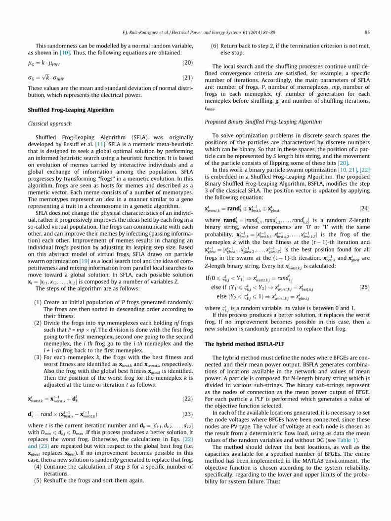
A transmission line can be represented by a number of separateelements in series or parallel or any combination thereof, depend-ing on the line. Fig. 1 shows a transmission line represented by aelements in series.
84 F.J. Ruiz-Rodriguez et al. / Electrical Power and Energy Systems 61 (2014) 81–89
Being kt and lt the ratios of failure and repair for component t,respectively. The availability of the component t is given by:
At ¼lt
kt þ ltð11Þ
and the probability of line failure is given by:
q ¼ 1�Ya
s¼1
As ð12Þ
The probability that line operates is the complement to 1 of (12):
p ¼ 1� q ð13Þ
Fig. 2. Cumulative distribution function for the tension in a generic node i.
Probability of occurrence for contingency
From the availability data (p) and non-availability (q) for eachline, the probability of contingency as a state of the system [9]can be determined. The states are the different configurations ofsystem that can be achieved by removing one or more lines.
The number of states depends on the number of lines of thesystem. For a system of L lines, the number of possible states is2L. The probability of occurrence for contingency m, P(m), or prob-ability of occurrence for a particular state (since there is a state inwhich there are no contingencies, everything operates fine) is
Pm ¼ po �Y
k20m
qk
pkð14Þ
where po is the probability for the normal state, calculated as,
po ¼YL
k¼1
pk ð15Þ
being 0m the set of lines involved in the contingency m.
Measurement of the probability of system failure
As mentioned above, it is considered that the system has failedafter a contingency if the limit of transmission capability of one ormore lines is exceeded or if the voltage of one or more nodes is out-side of the specified limits.
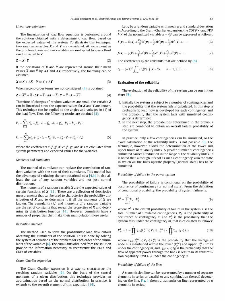
The probability that the power flow in a particular line does notexceed the limit of transmission capability can be determined di-rectly reading the cumulative distribution function for the powerflow in the line, according to the equation:
P½X 6 Lik� ¼Z Lik
�1f ðxÞdx ¼ FðLikÞ ð16Þ
where X is the random variable corresponding to the apparentpower flow in line ik, Lik is the limit of transmission capability ofthe line ik, f(x) is the PDF of apparent power flow in the line ik,and F(x) is the CDF of the apparent power flow in the line ik.
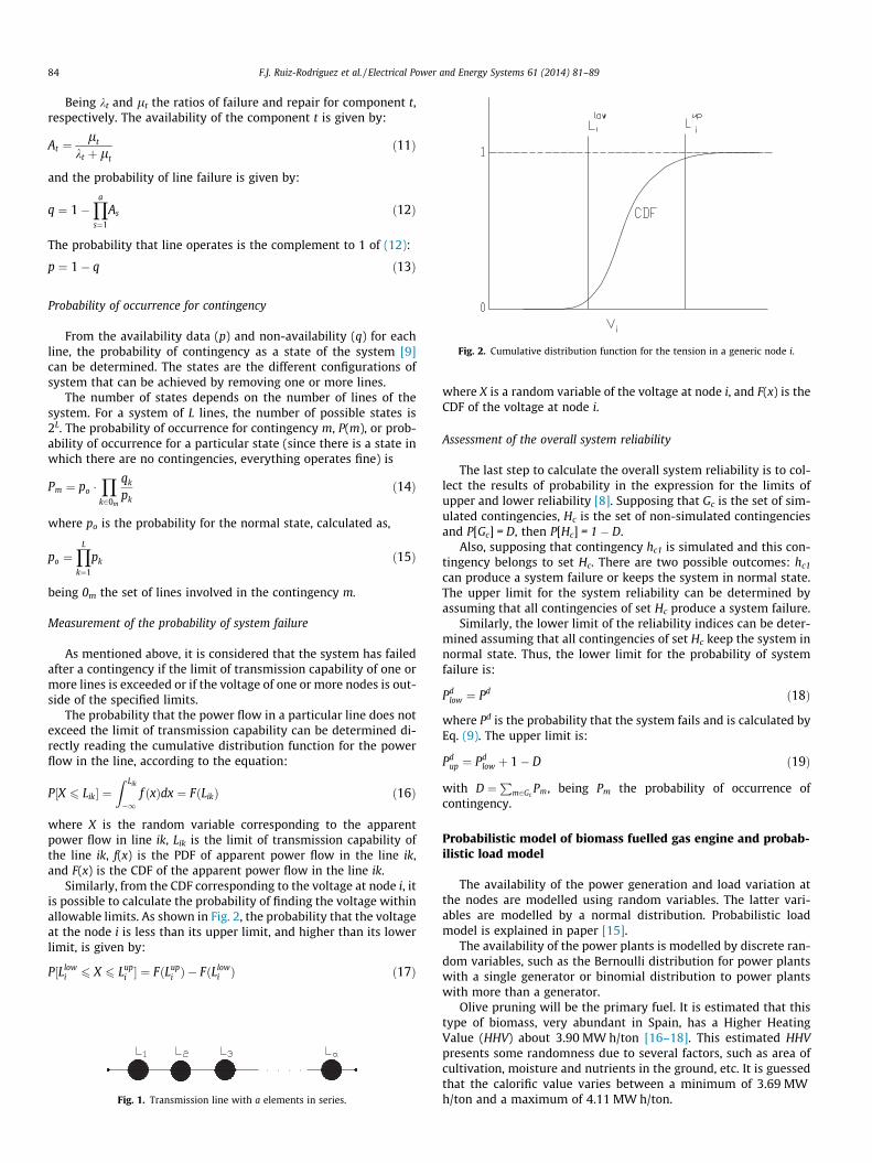
Similarly, from the CDF corresponding to the voltage at node i, itis possible to calculate the probability of finding the voltage withinallowable limits. As shown in Fig. 2, the probability that the voltageat the node i is less than its upper limit, and higher than its lowerlimit, is given by:
P½Llowi 6 X 6 Lup
i � ¼ FðLupi Þ � FðLlow
i Þ ð17Þ
Fig. 1. Transmission line with a elements in series.
where X is a random variable of the voltage at node i, and F(x) is theCDF of the voltage at node i.
Assessment of the overall system reliability
The last step to calculate the overall system reliability is to col-lect the results of probability in the expression for the limits ofupper and lower reliability [8]. Supposing that Gc is the set of sim-ulated contingencies, Hc is the set of non-simulated contingenciesand P[Gc] = D, then P[Hc] = 1 � D.
Also, supposing that contingency hc1 is simulated and this con-tingency belongs to set Hc. There are two possible outcomes: hc1
can produce a system failure or keeps the system in normal state.The upper limit for the system reliability can be determined byassuming that all contingencies of set Hc produce a system failure.
Similarly, the lower limit of the reliability indices can be deter-mined assuming that all contingencies of set Hc keep the system innormal state. Thus, the lower limit for the probability of systemfailure is:
Pdlow ¼ Pd ð18Þ
where Pd is the probability that the system fails and is calculated byEq. (9). The upper limit is:
Pdup ¼ Pd
low þ 1� D ð19Þ
with D ¼P
m2GcPm, being Pm the probability of occurrence of
contingency.
Probabilistic model of biomass fuelled gas engine and probab-ilistic load model
The availability of the power generation and load variation atthe nodes are modelled using random variables. The latter vari-ables are modelled by a normal distribution. Probabilistic loadmodel is explained in paper [15].
The availability of the power plants is modelled by discrete ran-dom variables, such as the Bernoulli distribution for power plantswith a single generator or binomial distribution to power plantswith more than a generator.
Olive pruning will be the primary fuel. It is estimated that thistype of biomass, very abundant in Spain, has a Higher HeatingValue (HHV) about 3.90 MW h/ton [16–18]. This estimated HHVpresents some randomness due to several factors, such as area ofcultivation, moisture and nutrients in the ground, etc. It is guessedthat the calorific value varies between a minimum of 3.69 MWh/ton and a maximum of 4.11 MW h/ton.
F.J. Ruiz-Rodriguez et al. / Electrical Power and Energy Systems 61 (2014) 81–89 85
This randomness can be modelled by a normal random variable,as shown in [10]. Thus, the following equations are obtained:
lG ¼ k � lHHV ð20Þ
rG ¼ffiffiffikp� rHHV ð21Þ
These values are the mean and standard deviation of normal distri-bution, which represents the electrical power.
Shuffled Frog-Leaping Algorithm
Classical approach
Shuffled Frog-Leaping Algorithm (SFLA) was originallydeveloped by Eusuff et al. [11]. SFLA is a memetic meta-heuristicthat is designed to seek a global optimal solution by performingan informed heuristic search using a heuristic function. It is basedon evolution of memes carried by interactive individuals and aglobal exchange of information among the population. SFLAprogresses by transforming ‘‘frogs’’ in a memetic evolution. In thisalgorithm, frogs are seen as hosts for memes and described as amemetic vector. Each meme consists of a number of memotypes.The memotypes represent an idea in a manner similar to a generepresenting a trait in a chromosome in a genetic algorithm.
SFLA does not change the physical characteristics of an individ-ual, rather it progressively improves the ideas held by each frog in aso-called virtual population. The frogs can communicate with eachother, and can improve their memes by infecting (passing informa-tion) each other. Improvement of memes results in changing anindividual frog’s position by adjusting its leaping step size. Basedon this abstract model of virtual frogs, SFLA draws on particleswarm optimization [19] as a local search tool and the idea of com-petitiveness and mixing information from parallel local searches tomove toward a global solution. In SFLA, each possible solutionxi ¼ ½xi;1; xi;2; . . . ; xi;Z � is composed by a number of variables Z.
The steps of the algorithm are as follows:
(1) Create an initial population of P frogs generated randomly.The frogs are then sorted in descending order according totheir fitness.
(2) Divide the frogs into mp memeplexes each holding nf frogssuch that P = mp � nf. The division is done with the first froggoing to the first memeplex, second one going to the secondmemeplex, the i-th frog go to the i-th memeplex and thei + 1-th frog back to the first memeplex.
(3) For each memeplex k, the frogs with the best fitness andworst fitness are identified as xbest,k and xworst,k respectively.Also the frog with the global best fitness xgbest is identified.Then the position of the worst frog for the memeplex k isadjusted at the time or iteration t as follows:
xtworst;k ¼ xt�1
worst;k þ dtk ð22Þ
dtk ¼ rand� ðxt�1
best;k � xt�1worst;kÞ ð23Þ
where t is the current iteration number and dk ¼ ½dk;1;dk;2; . . . ;dk;Z �with Dmin 6 dk;j 6 Dmax .If this process produces a better solution, itreplaces the worst frog. Otherwise, the calculations in Eqs. (22)and (23) are repeated but with respect to the global best frog (i.e.xgbest replaces xbest). If no improvement becomes possible in thiscase, then a new solution is randomly generated to replace that frog.
(4) Continue the calculation of step 3 for a specific number ofiterations.
(5) Reshuffle the frogs and sort them again.
(6) Return back to step 2, if the termination criterion is not met,else stop.
The local search and the shuffling processes continue until de-fined convergence criteria are satisfied, for example, a specificnumber of iterations. Accordingly, the main parameters of SFLAare: number of frogs, P, number of memeplexes, mp, number offrogs in each memeplex, nf, number of generation for eachmemeplex before shuffling, g, and number of shuffling iterations,tmax.
Proposed Binary Shuffled Frog-Leaping Algorithm
To solve optimization problems in discrete search spaces thepositions of the particles are characterized by discrete numberswhich can be binary. So that in these spaces, the position of a par-ticle can be represented by S length bits string, and the movementof the particle consists of flipping some of these bits [20].
In this work, a binary particle swarm optimization [10, 21], [22]is embedded in a Shuffled Frog-Leaping Algorithm. The proposedBinary Shuffled Frog-Leaping Algorithm, BSFLA, modifies the step3 of the classical SFLA. The position vector is updated by applyingthe following equation:
xtworst;k ¼ randt
k � xt�1best;k � xt
gbest ð24Þ
where randtk ¼ ½randt
k;1; randtk;2; . . . ; randt
k;Z � is a random Z-lengthbinary string, whose components are ’0’ or ’1’ with the sameprobability, xt�1
best;k ¼ ½xt�1best;k;1; x
t�1best;k;2; . . . ; xt�1
best;k;Z � is the frog of thememeplex k with the best fitness at the (t � 1)-th iteration andxt�1
gbest ¼ ½xt�1gbest;1; x
t�1gbest;2; . . . ; xt�1
gbest;Z � is the best position found for all
frogs in the swarm at the (t � 1)-th iteration. xt�1best;k and xt
gbest are
Z-length binary string. Every bit xtworst;k;j is calculated:
Ifð0 6 1tk;j < Y1Þ ) xt
worst;k;j ¼ randtk;j
else if ðY1 6 1tk;j < Y2Þ ) xt
worst;k;j ¼ xtbest;k;j
else ðY2 6 1tk;j 6 1Þ ) xt
worst;k;j ¼ xtgbest;j
ð25Þ
where 1tk;j is a random variable, its value is between 0 and 1.
If this process produces a better solution, it replaces the worstfrog. If no improvement becomes possible in this case, then anew solution is randomly generated to replace that frog.
The hybrid method BSFLA-PLF
The hybrid method must define the nodes where BFGEs are con-nected and their mean power output. BSFLA generates combina-tions of locations available in the network and values of meanpower. A particle is composed for N-length binary string which isdivided in various sub-strings. The binary sub-strings representas the nodes of connection as the mean power output of BFGE.For each particle a PLF is performed which generates a value ofthe objective function selected.
In each of the available locations generated, it is necessary to setthe node voltages where BFGEs have been connected, since thesenodes are PV type. The value of voltage at each node is chosen asthe result from a deterministic flow load, using as data the meanvalues of the random variables and without DG (see Table 1).
The method should deliver the best locations, as well as thecapacities available for a specified number of BFGEs. The entiremethod has been implemented in the MATLAB environment. Theobjective function is chosen according to the system reliability,specifically, regarding to the lower and upper limits of the proba-bility for system failure. Thus:
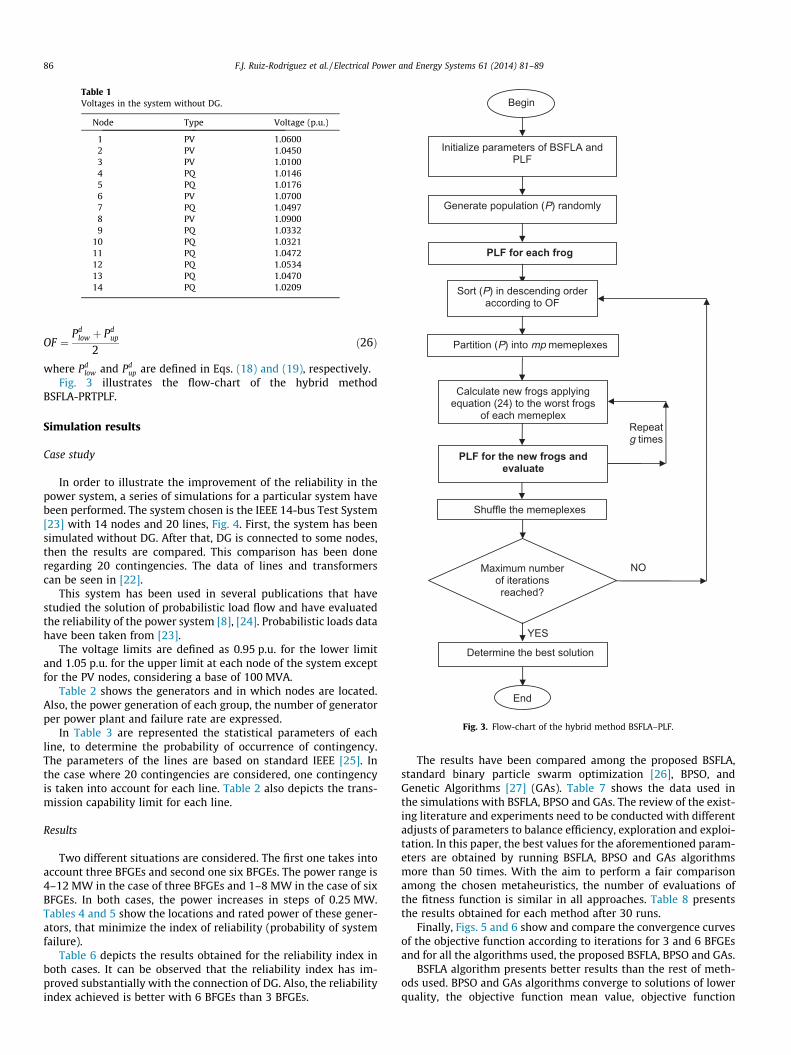
Table 1Voltages in the system without DG.
Node Type Voltage (p.u.)
1 PV 1.06002 PV 1.04503 PV 1.01004 PQ 1.01465 PQ 1.01766 PV 1.07007 PQ 1.04978 PV 1.09009 PQ 1.0332
10 PQ 1.032111 PQ 1.047212 PQ 1.053413 PQ 1.047014 PQ 1.0209
Begin
Initialize parameters of BSFLA and PLF
Generate population (P) randomly
PLF for each frog
Sort (P) in descending order according to OF
NO
Determine the best solution
Maximum number of iterations reached?
Shuffle the memeplexes
Partition (P) into mp memeplexes
YES
Calculate new frogs applying equation (24) to the worst frogs
of each memeplex
PLF for the new frogs and evaluate
Repeat g times
End
Fig. 3. Flow-chart of the hybrid method BSFLA–PLF.
86 F.J. Ruiz-Rodriguez et al. / Electrical Power and Energy Systems 61 (2014) 81–89
OF ¼Pd
low þ Pdup
2ð26Þ
where Pdlow and Pd
up are defined in Eqs. (18) and (19), respectively.Fig. 3 illustrates the flow-chart of the hybrid method
BSFLA-PRTPLF.
Simulation results
Case study
In order to illustrate the improvement of the reliability in thepower system, a series of simulations for a particular system havebeen performed. The system chosen is the IEEE 14-bus Test System[23] with 14 nodes and 20 lines, Fig. 4. First, the system has beensimulated without DG. After that, DG is connected to some nodes,then the results are compared. This comparison has been doneregarding 20 contingencies. The data of lines and transformerscan be seen in [22].
This system has been used in several publications that havestudied the solution of probabilistic load flow and have evaluatedthe reliability of the power system [8], [24]. Probabilistic loads datahave been taken from [23].
The voltage limits are defined as 0.95 p.u. for the lower limitand 1.05 p.u. for the upper limit at each node of the system exceptfor the PV nodes, considering a base of 100 MVA.
Table 2 shows the generators and in which nodes are located.Also, the power generation of each group, the number of generatorper power plant and failure rate are expressed.
In Table 3 are represented the statistical parameters of eachline, to determine the probability of occurrence of contingency.The parameters of the lines are based on standard IEEE [25]. Inthe case where 20 contingencies are considered, one contingencyis taken into account for each line. Table 2 also depicts the trans-mission capability limit for each line.
Results
Two different situations are considered. The first one takes intoaccount three BFGEs and second one six BFGEs. The power range is4–12 MW in the case of three BFGEs and 1–8 MW in the case of sixBFGEs. In both cases, the power increases in steps of 0.25 MW.Tables 4 and 5 show the locations and rated power of these gener-ators, that minimize the index of reliability (probability of systemfailure).
Table 6 depicts the results obtained for the reliability index inboth cases. It can be observed that the reliability index has im-proved substantially with the connection of DG. Also, the reliabilityindex achieved is better with 6 BFGEs than 3 BFGEs.
The results have been compared among the proposed BSFLA,standard binary particle swarm optimization [26], BPSO, andGenetic Algorithms [27] (GAs). Table 7 shows the data used inthe simulations with BSFLA, BPSO and GAs. The review of the exist-ing literature and experiments need to be conducted with differentadjusts of parameters to balance efficiency, exploration and exploi-tation. In this paper, the best values for the aforementioned param-eters are obtained by running BSFLA, BPSO and GAs algorithmsmore than 50 times. With the aim to perform a fair comparisonamong the chosen metaheuristics, the number of evaluations ofthe fitness function is similar in all approaches. Table 8 presentsthe results obtained for each method after 30 runs.
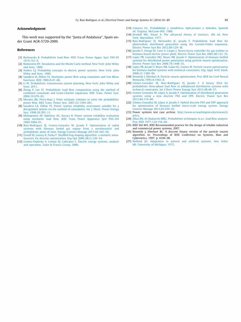
Finally, Figs. 5 and 6 show and compare the convergence curvesof the objective function according to iterations for 3 and 6 BFGEsand for all the algorithms used, the proposed BSFLA, BPSO and GAs.
BSFLA algorithm presents better results than the rest of meth-ods used. BPSO and GAs algorithms converge to solutions of lowerquality, the objective function mean value, objective function
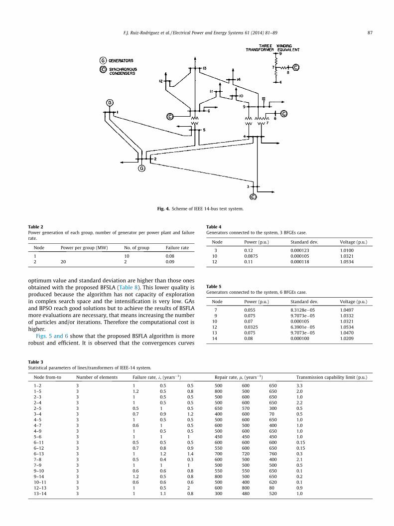
Fig. 4. Scheme of IEEE 14-bus test system.
Table 2Power generation of each group, number of generator per power plant and failurerate.
Node Power per group (MW) No. of group Failure rate
1 10 0.082 20 2 0.09
Table 4Generators connected to the system, 3 BFGEs case.
Node Power (p.u.) Standard dev. Voltage (p.u.)
3 0.12 0.000123 1.010010 0.0875 0.000105 1.032112 0.11 0.000118 1.0534
Table 5Generators connected to the system, 6 BFGEs case.
Node Power (p.u.) Standard dev. Voltage (p.u.)
7 0.055 8.3128e�05 1.04979 0.075 9.7073e�05 1.0332
10 0.07 0.000105 1.032112 0.0325 6.3901e�05 1.053413 0.075 9.7073e�05 1.047014 0.08 0.000100 1.0209
F.J. Ruiz-Rodriguez et al. / Electrical Power and Energy Systems 61 (2014) 81–89 87
optimum value and standard deviation are higher than those onesobtained with the proposed BFSLA (Table 8). This lower quality isproduced because the algorithm has not capacity of explorationin complex search space and the intensification is very low. GAsand BPSO reach good solutions but to achieve the results of BSFLAmore evaluations are necessary, that means increasing the numberof particles and/or iterations. Therefore the computational cost ishigher.
Figs. 5 and 6 show that the proposed BSFLA algorithm is morerobust and efficient. It is observed that the convergences curves
Table 3Statistical parameters of lines/transformers of IEEE-14 system.
Node from-to Number of elements Failure rate, k, (years�1) Repair rate, l, (years�1) Transmission capability limit (p.u.)
1–2 3 1 0.5 0.5 500 600 650 3.31–5 3 1.2 0.5 0.8 800 500 650 2.02–3 3 1 0.5 0.5 500 600 650 1.02–4 3 1 0.5 0.5 500 600 650 2.22–5 3 0.5 1 0.5 650 570 300 0.53–4 3 0.7 0.9 1.2 400 600 70 0.54–5 3 1 0.5 0.5 500 600 650 1.04–7 3 0.6 1 0.5 600 500 400 1.04–9 3 1 0.5 0.5 500 600 650 1.05–6 3 1 1 1 450 450 450 1.06–11 3 0.5 0.5 0.5 600 600 600 0.156–12 3 0.7 0.8 0.9 550 600 650 0.156–13 3 1 1.2 1.4 700 720 760 0.37–8 3 0.5 0.4 0.3 600 500 400 2.17–9 3 1 1 1 500 500 500 0.59–10 3 0.6 0.6 0.8 550 550 650 0.19–14 3 1.2 0.5 0.8 800 500 650 0.210–11 3 0.6 0.6 0.6 500 400 620 0.112–13 3 1 0.5 2 600 800 80 0.913–14 3 1 1.1 0.8 300 480 520 1.0
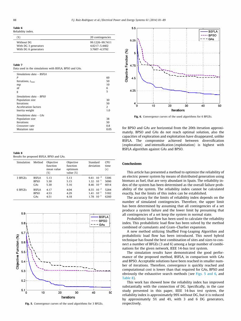
Table 6Reliability index.
(%) 20 contingencies
Without DG 99.1226–99.7411With DG 3 generators 4.8217–5.4402With DG 6 generators 3.7607–4.3792
Table 7Data used in the simulations with BSFLA, BPSO and GAs.
Simulations data – BSFLAP 60Iterations, tmax 50mp 10nf 6g 5
Simulations data – BPSOPopulation size 30Iterations 50Acceleration factors 2Inertia weight 1.0
Simulations data – GAsPopulation size 38Iterations 50Crossover rate 0.8Mutation rate 0.05
Table 8Results for proposed BSFLA, BPSO and GAs.
Simulation Method Objectivefunctionmean value(%)
Objectivefunctionoptimumvalue (%)
Standarddeviation
CPUtime(s)
3 BFGEs BSFLA 5.13 5.13 9.41 � 10�4 5306BPSO 5.30 5.15 1.32 � 10�1 5090GAs 5.30 5.16 8.46 � 10�2 6014
6 BFGEs BSFLA 4.17 4.04 8.55 � 10�2 5284BPSO 4.53 4.29 1.41 � 10�1 5182GAs 4.51 4.18 1.78 � 10�1 6260
Fig. 5. Convergence curves of the used algorithms for 3 BFGEs.
Fig. 6. Convergence curves of the used algorithms for 6 BFGEs.
88 F.J. Ruiz-Rodriguez et al. / Electrical Power and Energy Systems 61 (2014) 81–89
for BPSO and GAs are horizontal from the 20th iteration approxi-mately. BPSO and GAs do not reach optimal solution, also thecapacities of exploration and exploitation have disappeared, unlikeBSFLA. The compromise achieved between diversification(exploration) and intensification (exploitation) is highest withBSFLA algorithm against GAs and BPSO.
Conclusions
This article has presented a method to optimize the reliability ofan electric power system by means of distributed generation usingbiomass as fuel, that are very abundant in Spain. The reliability in-dex of the system has been determined as the overall failure prob-ability of the system. The reliability index cannot be calculatedexactly, but the limits of this index can be established.
The accuracy for the limits of reliability index depends on thenumber of simulated contingencies. Therefore, the upper limithas been determined by assuming that all contingencies of a setproduce a system failure and the lower limit by presuming thatall contingencies of a set keep the system in normal state.
Probabilistic load flow has been used to calculate the reliabilityindex. This probabilistic load flow has been solved by the methodcombined of cumulants and Gram–Charlier expansion.
A new method utilizing Shuffled Frog-Leaping Algorithm andprobabilistic load flow has been introduced. This novel hybridtechnique has found the best combination of sites and sizes to con-nect a number of BFGEs (3 and 6) among a large number of combi-nations for the given network, IEEE 14-bus test system.
The simulation results have demonstrated the good perfor-mance of the proposed method, BSFLA, in comparison with GAsand BPSO. Acceptable solutions have been reached in smaller num-ber of iterations. Therefore, convergence is quickly reached andcomputational cost is lower than that required for GAs, BPSO andobviously the exhaustive search methods (see Figs. 5 and 6, andTable 8).
This work has showed how the reliability index has improvedsubstantially with the connection of DG. Specifically, in the casestudy presented in this paper, IEEE 14-bus test system, thereliability index is approximately 99% without DG, but it is reducedby approximately 5% and 4%, with 3 and 6 DG generators,respectively.
F.J. Ruiz-Rodriguez et al. / Electrical Power and Energy Systems 61 (2014) 81–89 89
Acknowledgment
This work was supported by the ‘‘Junta of Andalusia’’, Spain un-der Grant AGR-5720-2009.
References
[1] Borkowska B. Probabilistic load flow. IEEE Trans. Power Appar. Syst. PAS-931974:752–9.
[2] Rubinstein RY. Simulation and the Monte Carlo method. New York: John Wileyand Sons; 1989.
[3] Anders GJ. Probability concepts in electric power systems. New York: JohnWiley and Sons; 1990.
[4] Sanabria IA, Dillon TS. Stochastic power flow using cumulants and Von Misesfunctions. IEEE 1986;8:47–60.
[5] Li W. Probabilistic transmission system planning. New York: John Wiley andSons; 2011.
[6] Zhang P, Lee ST. Probabilistic load flow computation using the method ofcombined cumulants and Gram-Charlier expansion. IEEE Trans. Power Syst.2004;19:676–82.
[7] Morales JM, Pérez-Ruiz J. Point estimate schemes to solve the probabilisticpower flow. IEEE Trans. Power Syst. 2007;22:1594–601.
[8] Sanabria LA, Dillon TS. Power system reliability assessment suitable for aderegulated system via the method of cumulantes. Int. J. Electr. Power EnergySyst. 1998;20:203–11.
[9] Meliopoulos AP, Bakirtzis AG, Kovacs R. Power system reliability evaluationusing stochastic load flow. IEEE Trans Power Apparatus Syst PAS-1031984:1084–91.
[10] Ruiz-Rodriguez FJ, Gomez-Gonzalez M, Jurado F. Optimization of radialsystems with biomass fueled gas engine from a metaheuristic andprobabilistic point of view. Energy Convers Manage 2013;65:343–50.
[11] Eusuff M, Lansey K, Pasha F. Shuffled frog-leaping algorithm: a memetic meta-heuristic for discrete optimization. Eng Opt 2006;38(2):129–54.
[12] Gomez-Expósito A, Conejo AJ, Cañizares C. Electric energy systems, analysisand operation. Tailor & Francis Group; 2009.
[13] Canavos GC. Probabilidad y estadística. Aplicaciones y métodos. Spanished. Virginia: McGraw-Hill; 1988.
[14] Kendall MG, Stuart A. The advanced theory of statistics. 4th ed. NewYork: Macmillan; 1977.
[15] Ruiz-Rodriguez FJ, Hernandez JC, Jurado F. Probabilistic load flow forphotovoltaic distributed generation using the Cornish-Fisher expansion.Electric Power Syst Res 2012;89:129–38.
[16] Jurado F, Ortega M, Cano A, Carpio J. Neuro-fuzzy controller for gas turbine inbiomass-based electric power plant. Electric Power Syst Res 2002;60:123–35.
[17] Lopez PR, González MG, Reyes NR, Jurado F. Optimization of biomass fuelledsystems for distributed power generation using particle swarm optimization.Electric Power Syst Res 2008;78:1448–55.
[18] Lopez PR, Jurado F, Reyes NR, Galan SG, Gomez M. Particle swarm optimizationfor biomass-fuelled systems with technical constraints. Eng. Appl. Artif. Intell.2008;21:1389–96.
[19] Kennedy J, Eberhart R. Particle swarm optimization. Proc IEEE Int Conf NeuralNetworks 1995;4:1942–8.
[20] Gómez-González M, Ruiz-Rodríguez FJ, Jurado F. A binary SFLA forprobabilistic three-phase load flow in unbalanced distribution systems withtechnical constraints. Int J Electr Power Energy Syst 2013;48:48–57.
[21] Gomez-Gonzalez M, López A, Jurado F. Optimization of distributed generationsystems using a new discrete PSO and OPF. Electric Power Syst Res2012;84:174–80.
[22] Gómez-González M, López A, Jurado F. Hybrid discrete PSO and OPF approachfor optimization of biomass fuelled micro-scale energy system. EnergyConvers Manage 2013;65:539–45.
[23] Power systems test case archive. http://www.ee.washington.edu/research/pstca.
[24] Allan RN, Al-Shakarchi MRG. Probabilistic techniques in a.c. load flow analysis.Proc IEEE 1977;124:154–60.
[25] IEEE Std 493. IEEE Recommended practice for the design of reliable industrialand commercial power systems, 2007.
[26] Kennedy J, Eberhart RC. A discrete binary version of the particle swarmalgorithm. In: Proceedings of IEEE Conference on Systems, Man andCybernetics, 1997. p. 4104–08.
[27] Holland JH. Adaptation in natural and artificial systems. Ann ArborMI: University of Michigan; 1975.