Resolving the Interactions between the Balance of Plant, SOFC, Power-Conditioning, and Application Loads

Project Investigators• Sudip K. Mazumder, Kaustuva Acharya, and Sanjaya Pradhan

(University of Illinois)• Michael von Spakovsky, Diego Rancruel, and Doug Nelson

(Virginia Tech)• Comas Haynes and Robert Williams

(Georgia Tech.)• Joseph Hartvigsen and S. Elangovan

(Ceramatec Inc.)• Chuck Mckintyre and Dan Herbison

(Synopsys Inc.)

SECA Core Technology Program Review MeetingMay 12, 2004

Boston, Massachusetts

PES Modeling &System Integration and Analysis

University of Illinois at Chicago

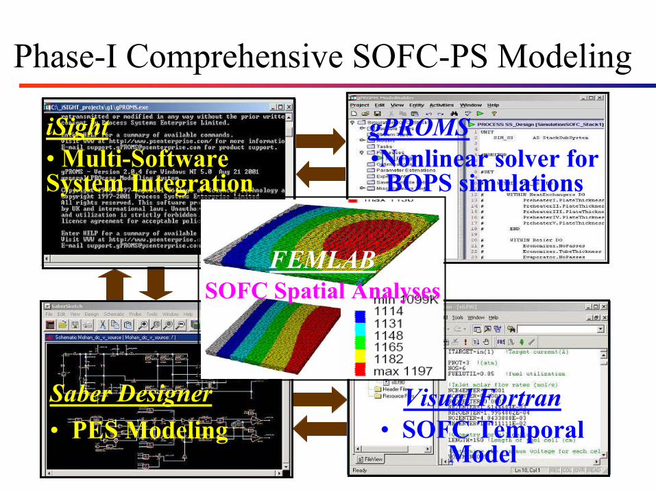
Phase-I Comprehensive SOFC-PS Modeling

Visual Fortran• SOFC Temporal

Model

gPROMS•Nonlinear solver for

BOPS simulations

iSight• Multi-Software System Integration

Saber Designer• PES Modeling

FEMLABSOFC Spatial Analyses

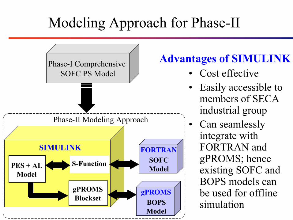
Modeling Approach for Phase-II

Phase-I Comprehensive SOFC PS Model

PES + ALModel

S-Function SOFCModel

FORTRAN

BOPSModel

gPROMSgPROMSBlockset

SIMULINK

Phase-II Modeling Approach

• Cost effective• Easily accessible to

members of SECA industrial group

• Can seamlessly integrate with FORTRAN and gPROMS; hence existing SOFC and BOPS models can be used for offline simulation

Advantages of SIMULINK

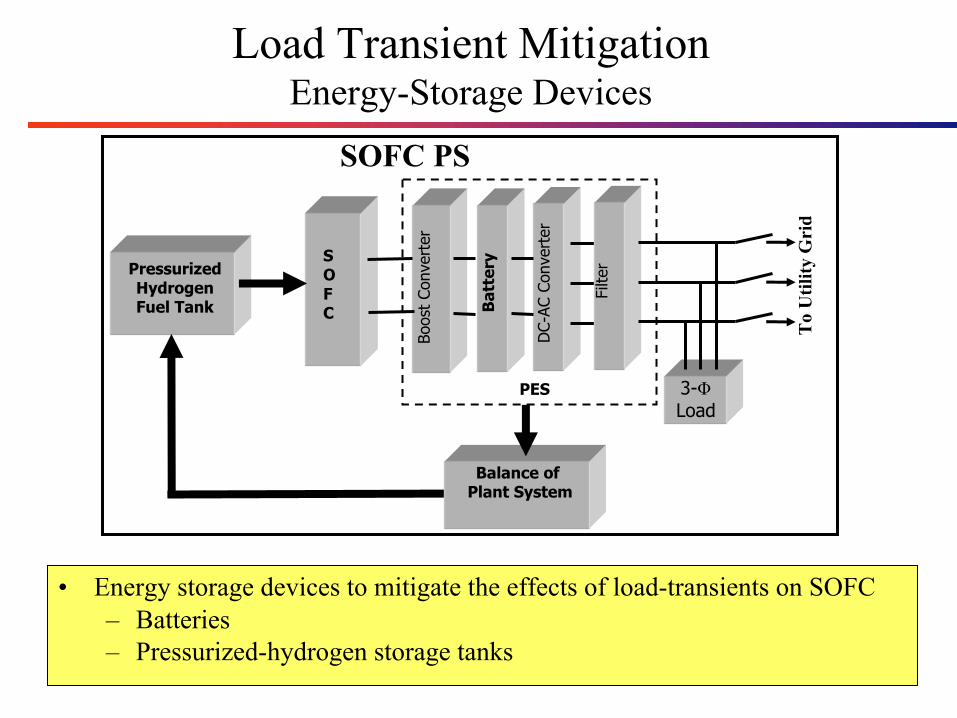
Load Transient MitigationEnergy-Storage Devices

• Energy storage devices to mitigate the effects of load-transients on SOFC– Batteries– Pressurized-hydrogen storage tanks

SOFC

Boos

t Co

nver

ter

Bat

tery

DC-

AC C

onve

rter

3-ΦLoad

To

Util

ity G

rid

PES

Balance ofPlant System

PressurizedHydrogenFuel Tank

SOFC PS

Filte

r

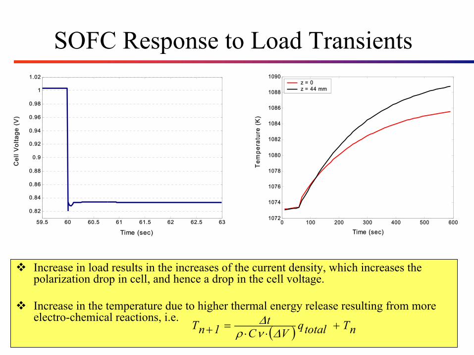
SOFC Response to Load Transients

0 100 200 300 400 500 6001072

1074

1076

1078

1080

1082

1084

1086

1088

1090

Time (sec)

Tem

pera

ture

(K

)

z = 0 z = 44 mm

59.5 60 60.5 61 61.5 62 62.5 63

0.82

0.84

0.86

0.88

0.9

0.92

0.94

0.96

0.98

1

1.02

Time (sec)

Cel

l Vol

tage

(V

)

Increase in load results in the increases of the current density, which increases the polarization drop in cell, and hence a drop in the cell voltage.

Increase in the temperature due to higher thermal energy release resulting from more electro-chemical reactions, i.e.

( ) nTtotalqVC

t1nT +

⋅⋅=+ ∆νρ

∆

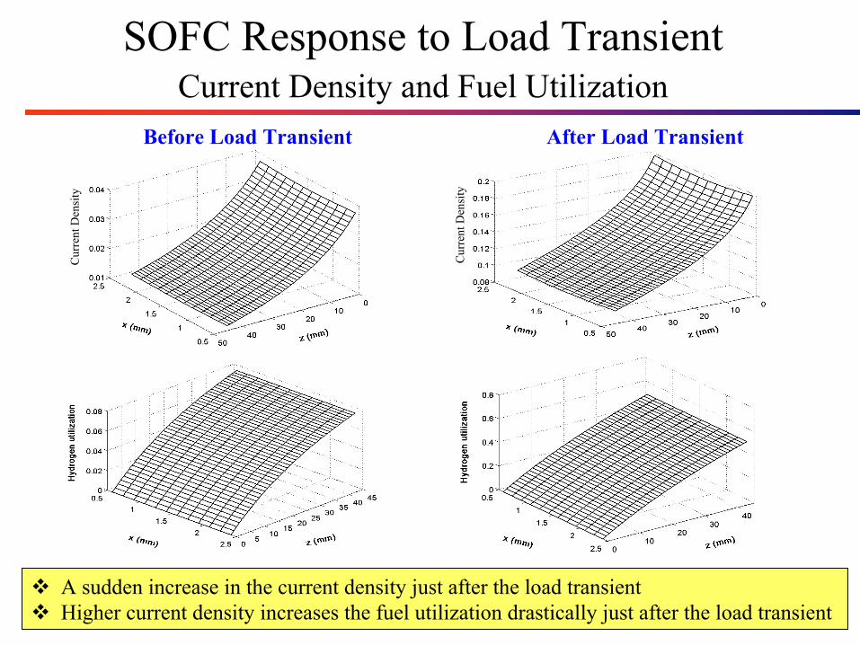
SOFC Response to Load TransientCurrent Density and Fuel Utilization

Before Load Transient After Load Transient

A sudden increase in the current density just after the load transient Higher current density increases the fuel utilization drastically just after the load transient

Cur

rent

Den

sity

Cur

rent

Den

sity

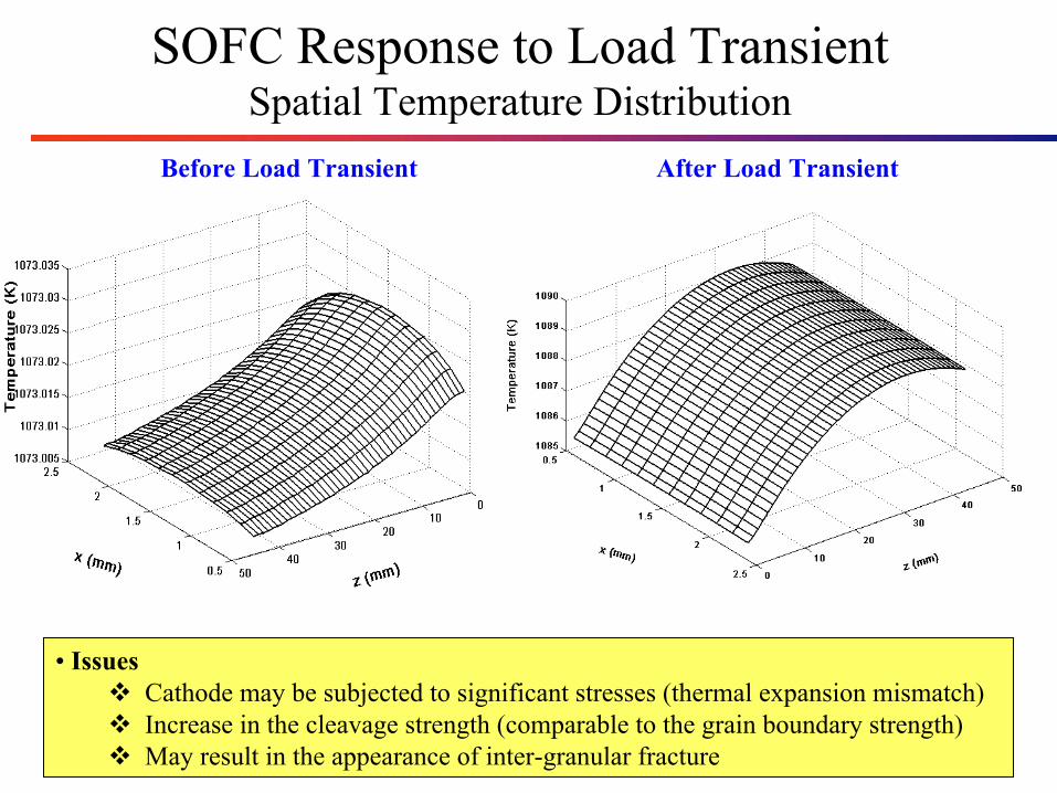
SOFC Response to Load TransientSpatial Temperature Distribution

• IssuesCathode may be subjected to significant stresses (thermal expansion mismatch)Increase in the cleavage strength (comparable to the grain boundary strength)May result in the appearance of inter-granular fracture

Before Load Transient After Load Transient

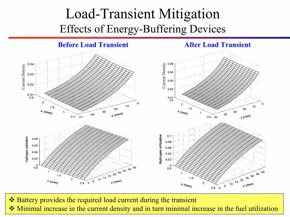
Load-Transient MitigationEffects of Energy-Buffering Devices

Battery provides the required load current during the transientMinimal increase in the current density and in turn minimal increase in the fuel utilization

Before Load Transient After Load Transient

Cur

rent

Den

sity

Cur

rent

Den

sity

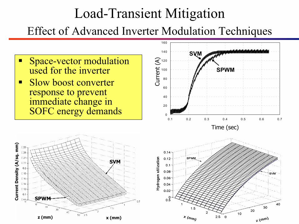
Load-Transient Mitigation Effect of Advanced Inverter Modulation Techniques

Space-vector modulation used for the inverter Slow boost converter response to prevent immediate change in SOFC energy demands 0

20

40

60

80

100

120

140

160

0.1 0.2 0.3 0.4 0.5 0.6 0.7

Time (sec)

Curr

ent

(A)

SPWM

SVM

z (mm) x (mm)

Cu

rren

t D

ensi

ty (

A/s

q. m

m)

SPWM

SVM

SOFCModeling and Analysis

Georgia Tech/Ceramatec

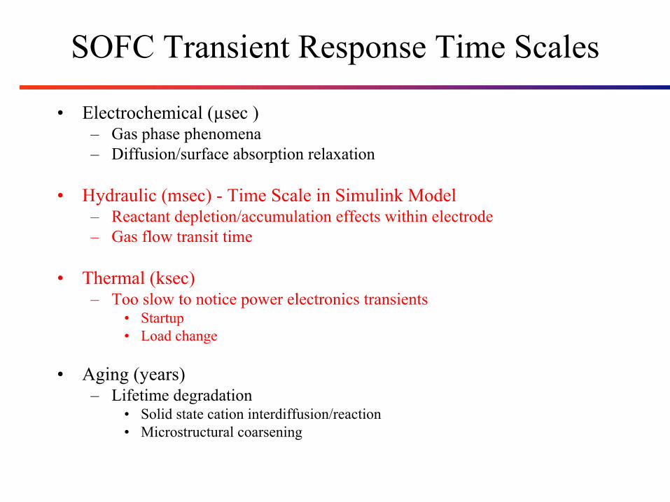
• Electrochemical (µsec )– Gas phase phenomena– Diffusion/surface absorption relaxation

• Hydraulic (msec) - Time Scale in Simulink Model– Reactant depletion/accumulation effects within electrode– Gas flow transit time

• Thermal (ksec)– Too slow to notice power electronics transients

• Startup• Load change

• Aging (years)– Lifetime degradation

• Solid state cation interdiffusion/reaction• Microstructural coarsening

SOFC Transient Response Time Scales

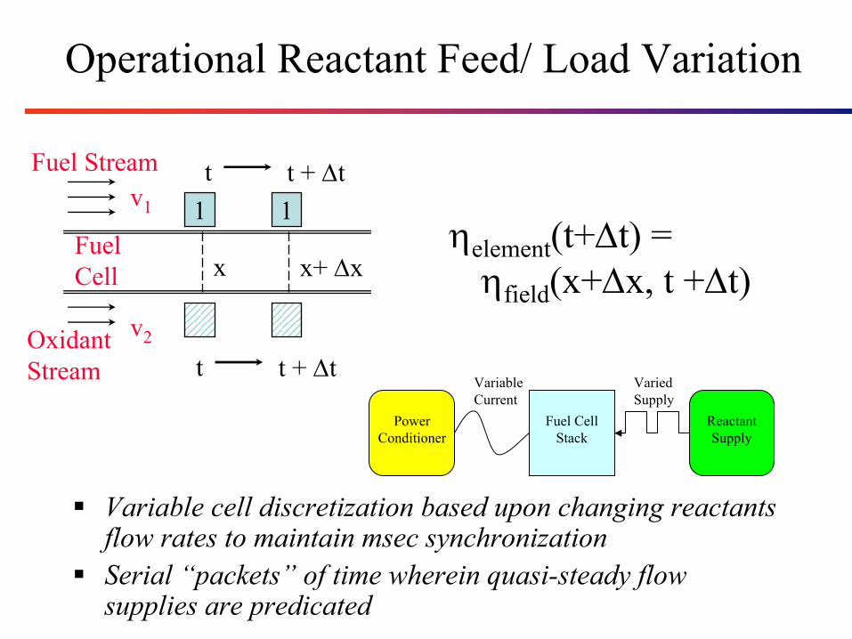
Operational Reactant Feed/ Load Variation

Variable cell discretization based upon changing reactants flow rates to maintain msec synchronizationSerial “packets” of time wherein quasi-steady flow supplies are predicated

Fuel Cell

11

Fuel Stream

Oxidant Stream

x

t + ∆t t

x+ ∆x

t t + ∆t v1

v2

ηelement(t+∆t) =ηfield(x+∆x, t +∆t)

Fuel CellStack

Power Conditioner

Reactant Supply

VariedSupply

Variable Current

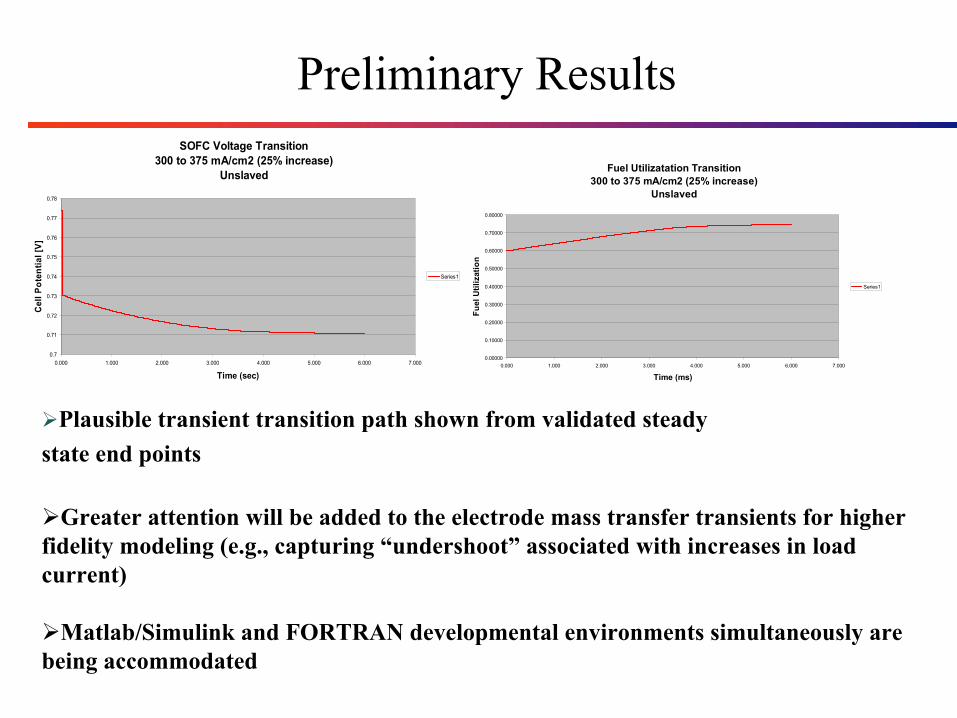
Preliminary ResultsSOFC Voltage Transition

300 to 375 mA/cm2 (25% increase)Unslaved

0.7

0.71

0.72

0.73

0.74

0.75

0.76

0.77

0.78

0.000 1.000 2.000 3.000 4.000 5.000 6.000 7.000

Time (sec)

Cel

l Pot

entia

l [V]

Series1

Fuel Utilizatation Transition300 to 375 mA/cm2 (25% increase)

Unslaved

0.00000

0.10000

0.20000

0.30000

0.40000

0.50000

0.60000

0.70000

0.80000

0.000 1.000 2.000 3.000 4.000 5.000 6.000 7.000

Time (ms)

Fuel

Util

izat

ion

Series1

Plausible transient transition path shown from validated steady state end points

Greater attention will be added to the electrode mass transfer transients for higher fidelity modeling (e.g., capturing “undershoot” associated with increases in load current)

Matlab/Simulink and FORTRAN developmental environments simultaneously are being accommodated

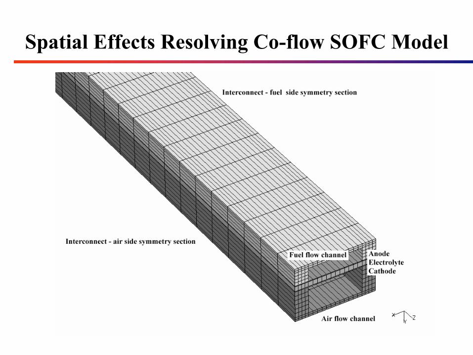
Spatial Effects Resolving Co-flow SOFC Model

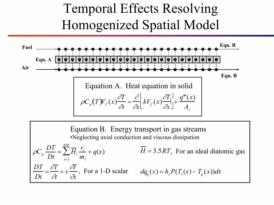
Temporal Effects Resolving Homogenized Spatial Model

ρCp T( )Vf (x)∂T∂t

=∂∂x

kVf (x)∂T∂x

+

′ ′ ′ q (x)Ac

Equation A. Heat equation in solid

Equation B. Energy transport in gas streams•Neglecting axial conduction and viscous dissipation

H = 3.5RT

dqg (x) = hcP(Ts (x) − Tg (x))dx

, For an ideal diatomic gasρCpDTDt

= H ii=1

nsp

∑ ri

mi

+ q(x)

DTDt

=∂T∂t

+ v∂T∂x

, For a 1-D scalar

Eqn. AAir

Fuel Eqn. B

Eqn. B

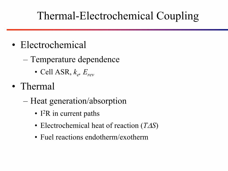
Thermal-Electrochemical Coupling

• Electrochemical– Temperature dependence

• Cell ASR, ke, Erev

• Thermal– Heat generation/absorption

• I2R in current paths• Electrochemical heat of reaction (T∆S)• Fuel reactions endotherm/exotherm

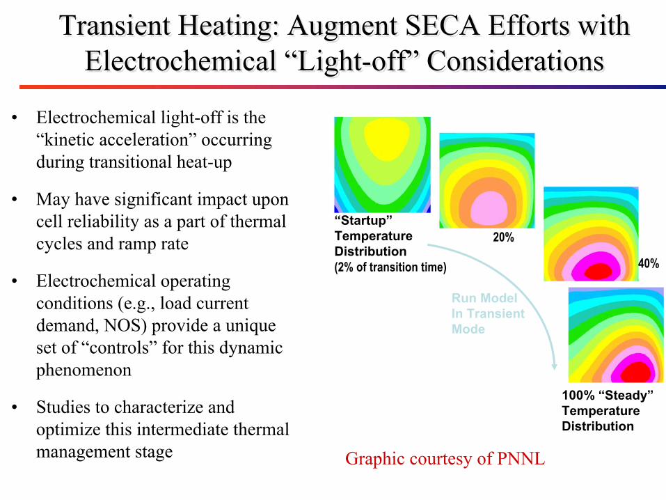
Transient Heating: Augment SECA Efforts with Electrochemical “Light-off” Considerations

Transient Heating: Augment SECA Efforts with Electrochemical “Light-off” Considerations

• Electrochemical light-off is the “kinetic acceleration” occurring during transitional heat-up

• May have significant impact upon cell reliability as a part of thermal cycles and ramp rate

• Electrochemical operating conditions (e.g., load current demand, NOS) provide a unique set of “controls” for this dynamic phenomenon

• Studies to characterize and optimize this intermediate thermal management stage

“Startup” TemperatureDistribution(2% of transition time)

100% “Steady” TemperatureDistribution

Run ModelIn TransientMode

20%

40%

Graphic courtesy of PNNL

Balance of Plant Sub-system (BOPS) Modeling and Analysis

Virginia Polytechnic Institute and State University

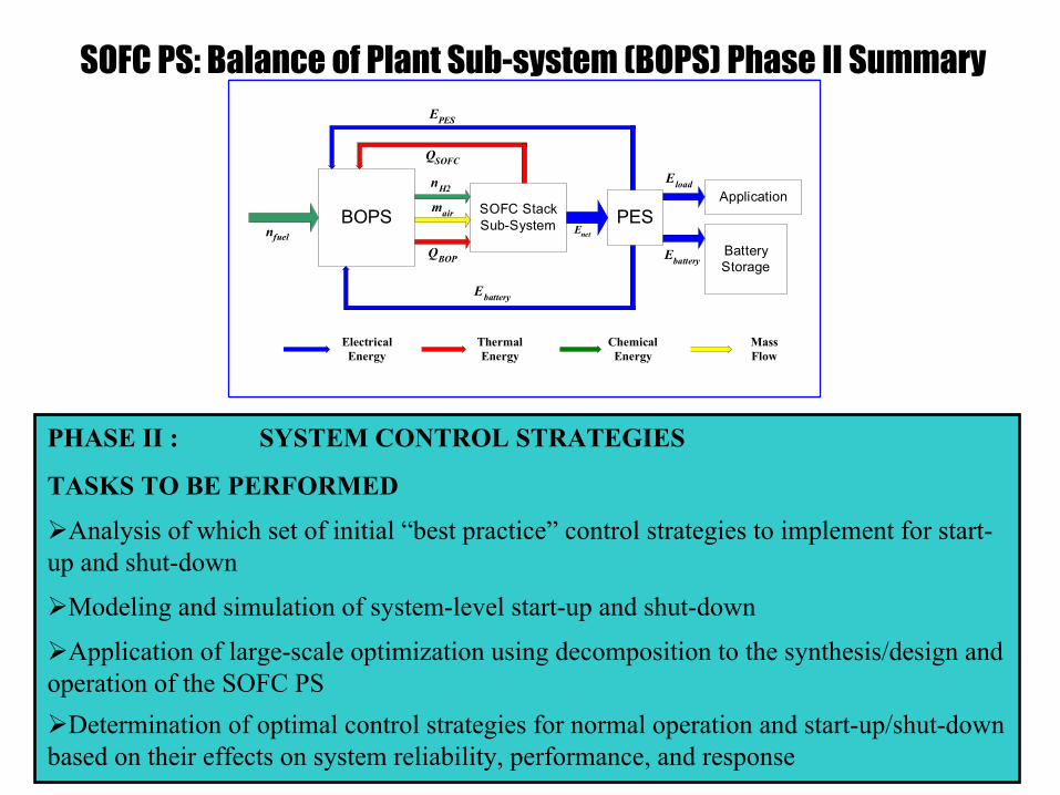
PHASE II : SYSTEM CONTROL STRATEGIES

TASKS TO BE PERFORMED

Analysis of which set of initial “best practice” control strategies to implement for start-up and shut-down

Modeling and simulation of system-level start-up and shut-down

Application of large-scale optimization using decomposition to the synthesis/design and operation of the SOFC PS

Determination of optimal control strategies for normal operation and start-up/shut-down based on their effects on system reliability, performance, and response

SOFC PS: Balance of Plant Sub-system (BOPS) Phase II Summary

BOPS SOFC StackSub-System PES

Application

BatteryStorage

nfuel

nH2

mair

QBOP

Enet

Eload

Ebattery

EPES

QSOFC

Ebattery

ElectricalEnergy

ThermalEnergy

ChemicalEnergy

MassFlow

BOPS SOFC StackSub-System PES

Application

BatteryStorage

nfuel

nH2

mair

QBOP

Enet

Eload

Ebattery

EPES

QSOFC

Ebattery

ElectricalEnergy

ThermalEnergy

ChemicalEnergy

MassFlow

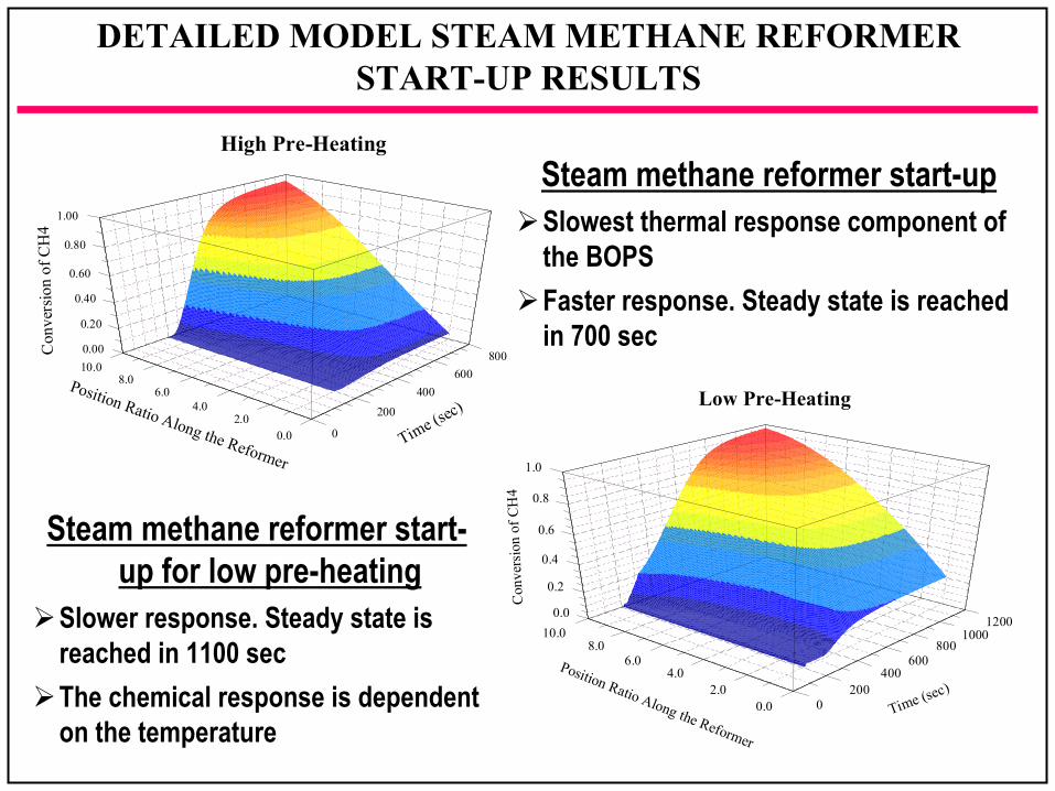
DETAILED MODEL STEAM METHANE REFORMER START-UP RESULTS

High Pre-Heating

Time (sec)

Position Ratio Along the Reformer

Con

vers

ion

of C

H4

0

200

400600

800

0.02.0

4.06.0

8.010.00.00

0.20

0.40

0.60

0.80

1.00

Steam methane reformer start-upSlowest thermal response component of the BOPSFaster response. Steady state is reached in 700 sec

Steam methane reformer start-up for low pre-heating

Slower response. Steady state is reached in 1100 secThe chemical response is dependent on the temperature

Low Pre-Heating

Time (sec)Position Ratio Along the Reformer

Con

vers

ion

of C

H4

0200

400600

8001000

1200

0.02.0

4.06.0

8.010.0

0.0

0.2

0.4

0.6

0.8

1.0

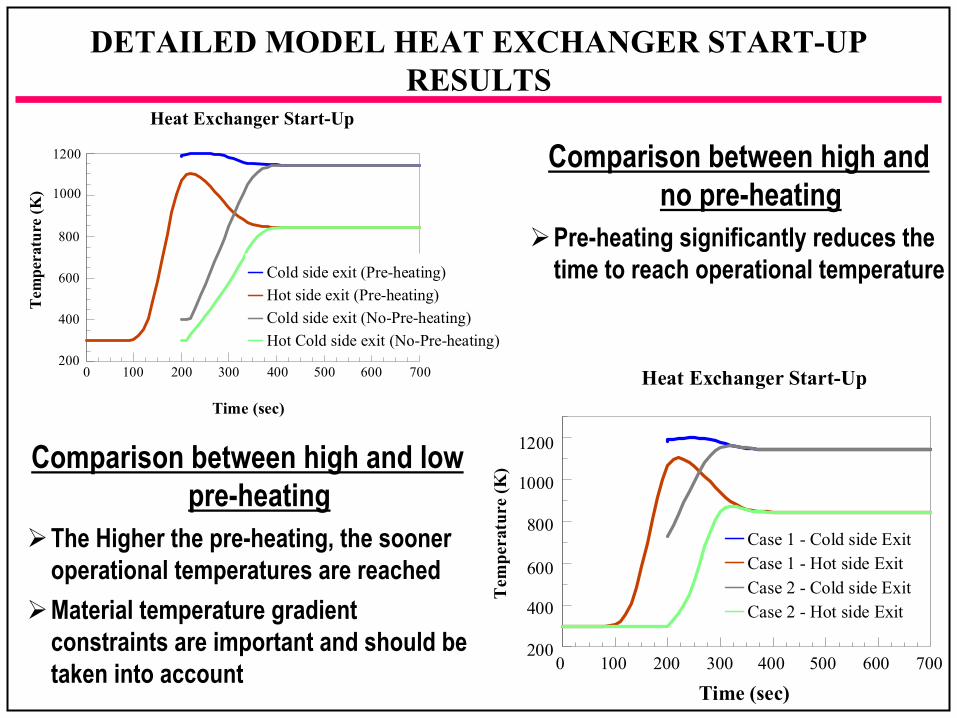
DETAILED MODEL HEAT EXCHANGER START-UP RESULTS

Time (sec)

0 100 200 300 400 500 600 700

Tem

pera

ture

(K)

200

400

600

800

1000

1200

Heat Exchanger Start-Up

Cold side exit (Pre-heating)Hot side exit (Pre-heating)Cold side exit (No-Pre-heating)Hot Cold side exit (No-Pre-heating)

Comparison between high and no pre-heating

Pre-heating significantly reduces the time to reach operational temperature

Comparison between high and low pre-heating

The Higher the pre-heating, the sooner operational temperatures are reachedMaterial temperature gradient constraints are important and should be taken into account

Heat Exchanger Start-Up

Time (sec)0 100 200 300 400 500 600 700

Tem

pera

ture

(K)

200

400

600

800

1000

1200

Case 1 - Cold side ExitCase 1 - Hot side ExitCase 2 - Cold side ExitCase 2 - Hot side Exit

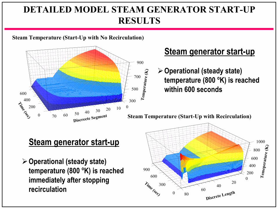
DETAILED MODEL STEAM GENERATOR START-UP RESULTS

Steam Temperature (Start-Up with No Recirculation)

Time (sec)

Discreete Segment

Tem

pera

ture

(K)

0

200400

600

010203040506070

300

500

700

900

Steam generator start-up

Operational (steady state) temperature (800 oK) is reached within 600 seconds

Steam generator start-up

Operational (steady state) temperature (800 oK) is reached immediately after stopping recirculation

Steam Temperature (Start-Up with Recirculation)

Time (sec)Discrete Length

Tem

eper

atur

e (K

)

0

300

600900

020

4060

80

200

400

600

800

1000

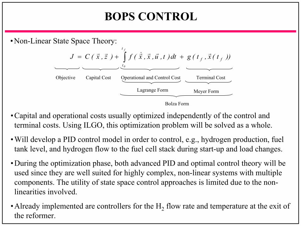
BOPS CONTROL

•Capital and operational costs usually optimized independently of the control and terminal costs. Using ILGO, this optimization problem will be solved as a whole.

•Will develop a PID control model in order to control, e.g., hydrogen production, fuel tank level, and hydrogen flow to the fuel cell stack during start-up and load changes.

•During the optimization phase, both advanced PID and optimal control theory will be used since they are well suited for highly complex, non-linear systems with multiple components. The utility of state space control approaches is limited due to the non-linearities involved.

•Already implemented are controllers for the H2 flow rate and temperature at the exit of the reformer.

))t(x,t(gdt)t,u,x,x(f)z,x(CJ ff

t

t

f

0

rrr&rrr++= ∫

Objective Terminal CostOperational and Control CostCapital Cost

Lagrange Form Meyer Form

Bolza Form

•Non-Linear State Space Theory:

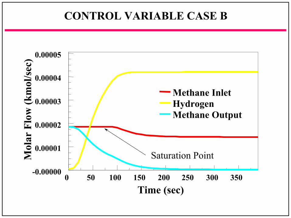
CONTROL VARIABLE CASE B

Time (sec)0 50 100 150 200 250 300 350

Mol

ar F

low

(km

ol/s

ec)

-0.00000

0.00001

0.00002

0.00003

0.00004

0.00005

Methane InletHydrogenMethane Output

Saturation Point

Time (sec)0 100 200 300 400 500

Pow

er (k

W)

0

1000

2000

3000

4000

5000

6000

Mol

ar F

low

(km

ol/s

ec)

-0.00000

0.00001

0.00002

0.00003

0.00004

0.00005

Mol

ar F

low

(km

ol/s

ec)

-0.00000

0.00001

0.00002

0.00003

0.00004

0.00005

PoweroutH2

m&

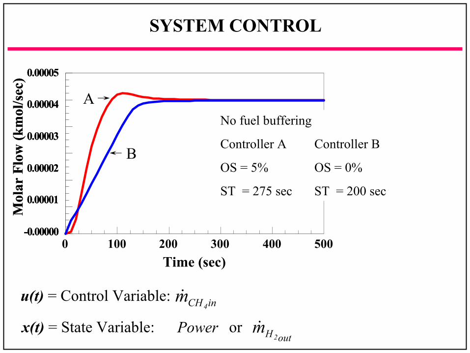
SYSTEM CONTROL

u(t) = Control Variable: inCH4m&

x(t) = State Variable: or

No fuel buffering

Controller A Controller B

OS = 5% OS = 0%

ST = 275 sec ST = 200 sec

A

B

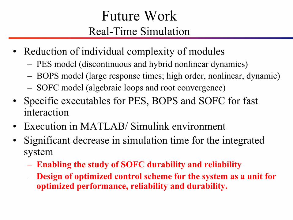
• Reduction of individual complexity of modules– PES model (discontinuous and hybrid nonlinear dynamics)– BOPS model (large response times; high order, nonlinear, dynamic)– SOFC model (algebraic loops and root convergence)

• Specific executables for PES, BOPS and SOFC for fast interaction

• Execution in MATLAB/ Simulink environment• Significant decrease in simulation time for the integrated

system– Enabling the study of SOFC durability and reliability– Design of optimized control scheme for the system as a unit for

optimized performance, reliability and durability.

Future WorkReal-Time Simulation

Future WorkPlanar Solid Oxide Fuel Cell (Planar SOFC)

• Planar SOFC stack model (electrical, thermal and electrochemical) development, enhancement and model validation– Georgia Tech & Cerametec

• Implementation and validation of a comprehensive balance of plant system model (thermodynamic, kinetic, and geometric) and optimal control strategies (bottoms-up approach)– Virginia Tech & Cerametec

• Development of PES nonlinear topologies (stationary and non-stationary application loads)– U of I at Chicago

• System integration and interaction analyses – U of I at Chicago

Future WorkDevelopment of New Control Strategies

Optimal control strategies using a bottoms-up approach to improve BOPS response to load transients

Optimal balance between overall system efficiency, cost, and SOFC stack durability at each load point

Could lead to the control of each subsystem in such a way that the system responds optimally to any given load

Greater fidelity as a result of the rigorous simulation of the subsystems and a sufficient consideration of system dynamics