Distribution Statement A: Approved for Public Release

Results and Conclusions: Perception Sensor Study for High Speed

Autonomous Operations Anne Schneidera, Zachary LaCellea, Alberto Lacazea, Karl Murphya, Ryan Closeb

aRobotic Research, LLC, Gaithersburg, MD; bUS Army RDECOM CERDEC Night Vision and Electronic Sensors Directorate,

Fort Belvoir, VA

ABSTRACT

Previous research has presented work on sensor requirements, specifications, and testing, to evaluate the

feasibility of increasing autonomous vehicle system speeds. Discussions included the theoretical background for

determining sensor requirements, and the basic test setup and evaluation criteria for comparing existing and

prototype sensor designs. This paper will present and discuss the continuation of this work. In particular, this

paper will focus on analyzing the problem via a real-world comparison of various sensor technology testing

results, as opposed to previous work that utilized more of a theoretical approach. LADAR/LIDAR, radar, visual,

and infrared sensors are considered in this research. Results are evaluated against the theoretical, desired

perception specifications. Conclusions for utilizing a suite of perception sensors, to achieve the goal of doubling

ground vehicle speeds, is also discussed.

Keywords: Sensors, high-speed, autonomy, LADAR, LIDAR

1. INTRODUCTION

One of the most difficult challenges in the field of autonomous ground robotics is increasing the maximum

operational speed of vehicles. In order to safely increase speed, the vehicle must be able to perceive and make

decisions based upon the surrounding environment. Currently, state-of-the-art robotic systems utilize LADARs

(LAser Detection And Ranging), also referred to as LIDARs (LIght Detection And Ranging) as the primary

perception sensor. LADARs measure the distance to a point by emitting a laser beam and analyzing the reflected

light. Time-of-flight LADAR systems convert the roundtrip time of the laser (i.e., the time it takes the laser to

reach an object and reflect back to the sensor) into a distance measurement.

In [1], we presented the initial results from a sensor study aimed to analyze, both from a theoretical perspective

and using real-world data, what sensor specifications are required for high speed (i.e., 60mph) driving. This

initial portion of the study mostly focused on a theoretical analysis. While the derivation of these specifications

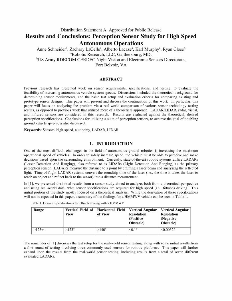
will not be repeated in this paper, a summary of the findings for a HMMWV vehicle can be seen in Table 1.

Table 1: Desired Specifications for 60mph driving with a HMMWV

Range Vertical Field of

View

Horizontal Field

of View

Vertical Angular

Resolution

(Positive

Obstacle)

Vertical Angular

Resolution

(Negative

Obstacle)

≥123m ≥123° ≥140° ≤0.1° ≤0.0032°

The remainder of [1] discusses the test setup for the real-world sensor testing, along with some initial results from

a first round of testing involving three commonly used sensors for robotic platforms. This paper will further

expand upon the results from the real-world sensor testing, including results from a total of seven different

evaluated LADARs.

2. SENSOR STUDY RESULTS

2.1. Evaluated LADAR Sensors

A variety of different LADAR sensors were tested in this study. The Velodyne HDL-64E S2, the GDRS

microLADAR, and the IBEO LUX 8L were chosen because each one has been utilized in major robotics projects

(e.g., the DARPA Urban Challenge, USASOC’s Small Unit Support IED-defeat (SUSI) program, TARDEC’s

Autonomous Mobility Applique System (AMAS)). Three other tested LADARs were manufactured by Optech,

and each are marketed towards different applications (the ILRIS-HD for surveying, the Lynx SG1 for mapping,

and the LRM is a prototype sensor for the Canadian Space Agency). The final tested sensor was the Neptec

OPAL-ECR, which is a newly developed sensor (available late 2015), designed for long range (>200m), real-time

scanning in harsh environments (such as mining and construction), and has obscurant penetration capabilities.

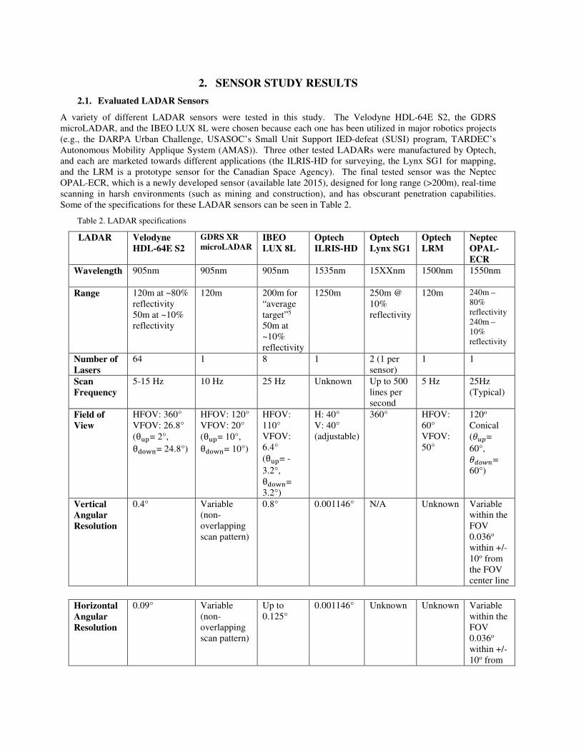
Some of the specifications for these LADAR sensors can be seen in Table 2.

Table 2. LADAR specifications

LADAR Velodyne

HDL-64E S2

GDRS XR

microLADAR IBEO

LUX 8L

Optech

ILRIS-HD

Optech

Lynx SG1

Optech

LRM

Neptec

OPAL-

ECR

Wavelength 905nm 905nm 905nm 1535nm

15XXnm 1500nm 1550nm

Range 120m at ~80%

reflectivity

50m at ~10%

reflectivity

120m 200m for

“average

target”5

50m at

~10%

reflectivity

1250m 250m @

10%

reflectivity

120m 240m –

80%

reflectivity

240m –

10%

reflectivity

Number of

Lasers

64 1 8 1 2 (1 per

sensor)

1 1

Scan

Frequency

5-15 Hz 10 Hz 25 Hz Unknown Up to 500

lines per

second

5 Hz 25Hz

(Typical)

Field of

View

HFOV: 360°

VFOV: 26.8°

(θ��= 2°,

θ����= 24.8°)

HFOV: 120°

VFOV: 20°

(θ��= 10°,

θ����= 10°)

HFOV:

110°

VFOV:

6.4°

(�= -

3.2°,

���=

3.2°)

H: 40°

V: 40°

(adjustable)

360° HFOV:

60°

VFOV:

50°

120o

Conical

(�=

60°,

��� �=

60°)

Vertical

Angular

Resolution

0.4° Variable

(non-

overlapping

scan pattern)

0.8° 0.001146° N/A Unknown Variable

within the

FOV

0.036o

within +/-

10o from

the FOV

center line

Horizontal

Angular

Resolution

0.09° Variable

(non-

overlapping

scan pattern)

Up to

0.125°

0.001146° Unknown Unknown Variable

within the

FOV

0.036o

within +/-

10o from

The Velodyne 64 returns many more points per second than the other LADARs being evaluated, in part because it

has multiple (64) scan lines. The 64 lasers are rotated to obtain a 360° horizontal field of view. The IBEO LUX

8L is also a multi-line scanner (it contains two groups of four lasers, each), but has a smaller vertical and

horizontal field of view than the Velodyne. The XR microLADAR and Neptec OPAL-ECR are unique, because

they feature non-overlapping scan patterns. A single laser is internally moved to allow for two degrees of

freedom – azimuth and elevation angle. This creates a non-overlapping scan pattern, which means that a very

dense point cloud can be created when the vehicle is not in motion. However, this can be a disadvantage at higher

speeds, as the sensors only have a single laser to cover the field of view, as compared to the multi-line scanners;

hence, they do not return as many points per second, leading to less dense point clouds.

The Neptec and Optech sensors operate in the SWIR wavelength, and are therefore capable of much longer ranges

than the more commonly used 905nm sensors. This is because the power can be increased on the SWIR lasers,

while still remaining eye-safe. The ILRIS scanner has the longest range (>1000m) of all the sensors being tested.

Additionally, the beam divergence is much smaller. However, because the sensor is designed for detailed

surveying applications, the scan times are relatively slow, which makes it less applicable for high speed platforms.

As we will discuss further in following sections, we were able to speed up the scans to some extent by reducing

the FOV and number of points returned per scan. The Lynx is a two-sensor system that is mounted on the back of

a vehicle. Each sensor has a single scan line, and is mounted at an angle, scanning to the side of the vehicle.

Because this is not a forward scanning LADAR, we adjusted some of the tests to be more appropriate for the scan

pattern. Lastly, the LRM is a prototype, 2-axis scanner developed for the Canadian Space Agency. This is the

only 2-axis scanner from Optech that was evaluated.

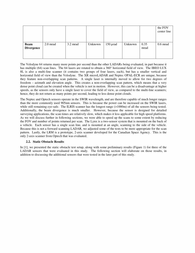
2.2. Static Obstacle Results

In [1], we presented the static obstacle test setup, along with some preliminary results (Figure 1) for three of the

LADAR sensors that were evaluated in this study. The following section will elaborate on those results, in

addition to discussing the additional sensors that were tested in the later part of this study.

the FOV

center line

Beam

Divergence

2.0 mrad 3.2 mrad Unknown 150 µrad Unknown 0.35

mrad

0.6 mrad

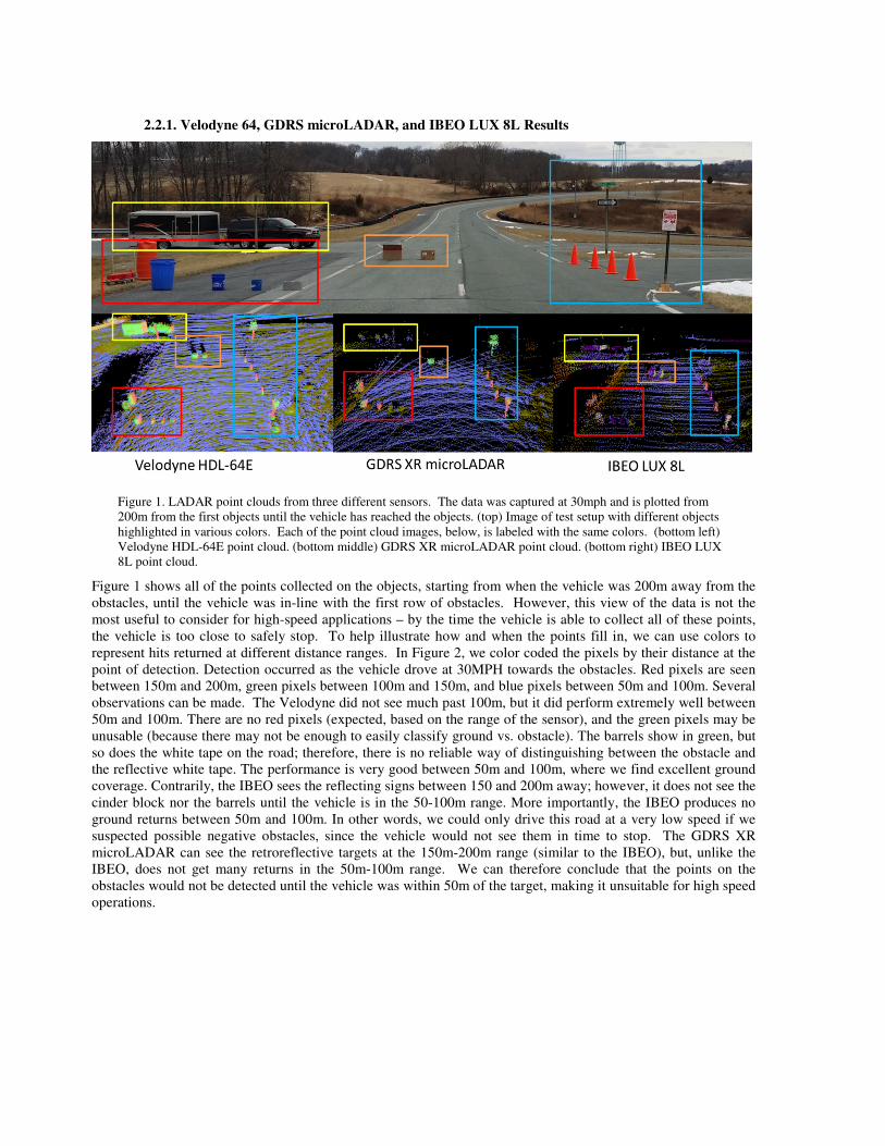
2.2.1. Velodyne 64, GDRS microLADAR, and IBEO LUX 8L Results

Figure 1. LADAR point clouds from three different sensors. The data was captured at 30mph and is plotted from

200m from the first objects until the vehicle has reached the objects. (top) Image of test setup with different objects

highlighted in various colors. Each of the point cloud images, below, is labeled with the same colors. (bottom left)

Velodyne HDL-64E point cloud. (bottom middle) GDRS XR microLADAR point cloud. (bottom right) IBEO LUX

8L point cloud.

Figure 1 shows all of the points collected on the objects, starting from when the vehicle was 200m away from the

obstacles, until the vehicle was in-line with the first row of obstacles. However, this view of the data is not the

most useful to consider for high-speed applications – by the time the vehicle is able to collect all of these points,

the vehicle is too close to safely stop. To help illustrate how and when the points fill in, we can use colors to

represent hits returned at different distance ranges. In Figure 2, we color coded the pixels by their distance at the

point of detection. Detection occurred as the vehicle drove at 30MPH towards the obstacles. Red pixels are seen

between 150m and 200m, green pixels between 100m and 150m, and blue pixels between 50m and 100m. Several

observations can be made. The Velodyne did not see much past 100m, but it did perform extremely well between

50m and 100m. There are no red pixels (expected, based on the range of the sensor), and the green pixels may be

unusable (because there may not be enough to easily classify ground vs. obstacle). The barrels show in green, but

so does the white tape on the road; therefore, there is no reliable way of distinguishing between the obstacle and

the reflective white tape. The performance is very good between 50m and 100m, where we find excellent ground

coverage. Contrarily, the IBEO sees the reflecting signs between 150 and 200m away; however, it does not see the

cinder block nor the barrels until the vehicle is in the 50-100m range. More importantly, the IBEO produces no

ground returns between 50m and 100m. In other words, we could only drive this road at a very low speed if we

suspected possible negative obstacles, since the vehicle would not see them in time to stop. The GDRS XR

microLADAR can see the retroreflective targets at the 150m-200m range (similar to the IBEO), but, unlike the

IBEO, does not get many returns in the 50m-100m range. We can therefore conclude that the points on the

obstacles would not be detected until the vehicle was within 50m of the target, making it unsuitable for high speed

operations.

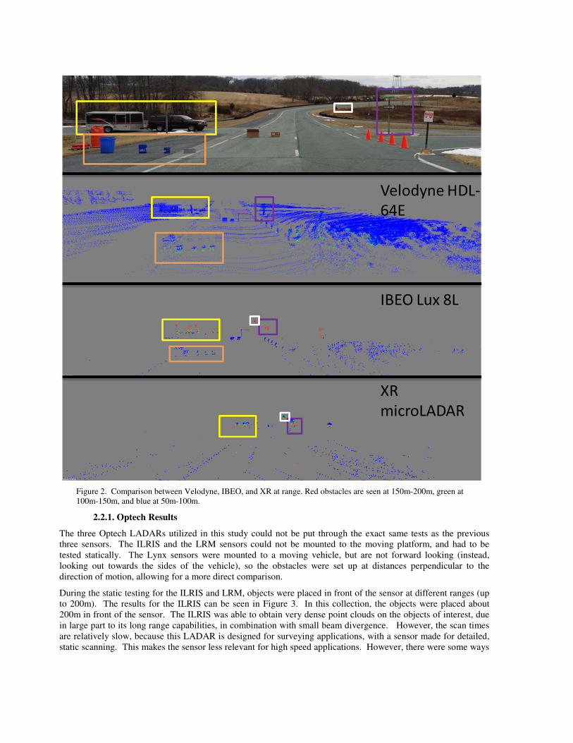
Figure 2. Comparison between Velodyne, IBEO, and XR at range. Red obstacles are seen at 150m-200m, green at

100m-150m, and blue at 50m-100m.

2.2.1. Optech Results

The three Optech LADARs utilized in this study could not be put through the exact same tests as the previous

three sensors. The ILRIS and the LRM sensors could not be mounted to the moving platform, and had to be

tested statically. The Lynx sensors were mounted to a moving vehicle, but are not forward looking (instead,

looking out towards the sides of the vehicle), so the obstacles were set up at distances perpendicular to the

direction of motion, allowing for a more direct comparison.

During the static testing for the ILRIS and LRM, objects were placed in front of the sensor at different ranges (up

to 200m). The results for the ILRIS can be seen in Figure 3. In this collection, the objects were placed about

200m in front of the sensor. The ILRIS was able to obtain very dense point clouds on the objects of interest, due

in large part to its long range capabilities, in combination with small beam divergence. However, the scan times

are relatively slow, because this LADAR is designed for surveying applications, with a sensor made for detailed,

static scanning. This makes the sensor less relevant for high speed applications. However, there were some ways

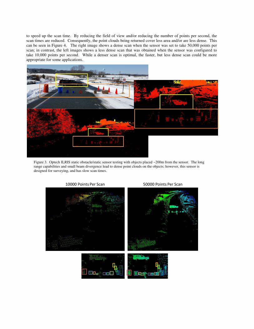
to speed up the scan time. By reducing the field of view and/or reducing the number of points per second, the

scan times are reduced. Consequently, the point clouds being returned cover less area and/or are less dense. This

can be seen in Figure 4. The right image shows a dense scan when the sensor was set to take 50,000 points per

scan; in contrast, the left images shows a less dense scan that was obtained when the sensor was configured to

take 10,000 points per second. While a denser scan is optimal, the faster, but less dense scan could be more

appropriate for some applications.

Figure 3. Optech ILRIS static obstacle/static sensor testing with objects placed ~200m from the sensor. The long

range capabilities and small beam divergence lead to dense point clouds on the objects; however, this sensor is

designed for surveying, and has slow scan times.

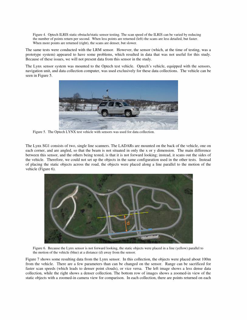
Figure 4. Optech ILRIS static obstacle/static sensor testing. The scan speed of the ILRIS can be varied by reducing

the number of points return per second. When less points are returned (left) the scans are less detailed, but faster.

When more points are returned (right), the scans are denser, but slower.

The same tests were conducted with the LRM sensor. However, the sensor (which, at the time of testing, was a

prototype system) appeared to have some problems, which resulted in data that was not useful for this study.

Because of these issues, we will not present data from this sensor in the study.

The Lynx sensor system was mounted to the Optech test vehicle. Optech’s vehicle, equipped with the sensors,

navigation unit, and data collection computer, was used exclusively for these data collections. The vehicle can be

seen in Figure 5.

Figure 5. The Optech LYNX test vehicle with sensors was used for data collection.

The Lynx SG1 consists of two, single line scanners. The LADARs are mounted on the back of the vehicle, one on

each corner, and are angled, so that the beam is not situated in only the x or y dimension. The main difference

between this sensor, and the others being tested, is that it is not forward looking; instead, it scans out the sides of

the vehicle. Therefore, we could not set up the objects in the same configuration used in the other tests. Instead

of placing the static objects across the road, the objects were placed along a line parallel to the motion of the

vehicle (Figure 6).

Figure 6. Because the Lynx sensor is not forward looking, the static objects were placed in a line (yellow) parallel to

the motion of the vehicle (blue) at a distance (d) away from the sensor.

Figure 7 shows some resulting data from the Lynx sensor. In this collection, the objects were placed about 100m

from the vehicle. There are a few parameters than can be changed on the sensor. Range can be sacrificed for

faster scan speeds (which leads to denser point clouds), or vice versa. The left image shows a less dense data

collection, while the right shows a denser collection. The bottom row of images shows a zoomed-in view of the

static objects with a zoomed-in camera view for comparison. In each collection, there are points returned on each

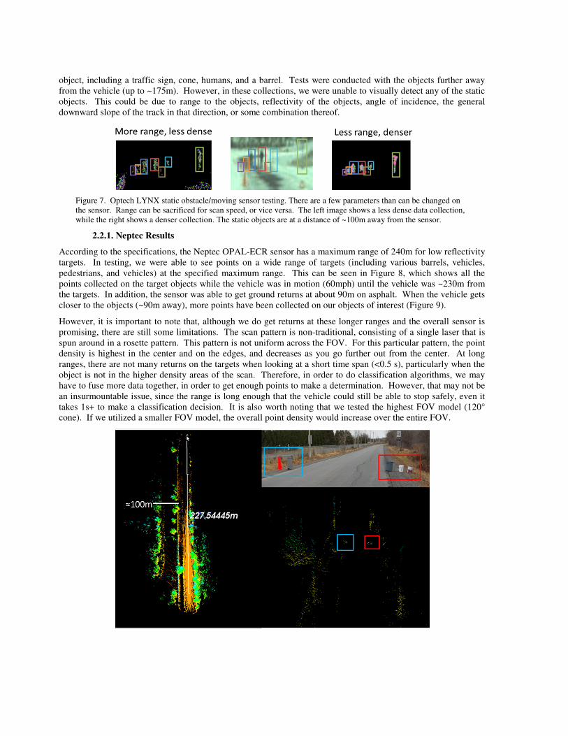
object, including a traffic sign, cone, humans, and a barrel. Tests were conducted with the objects further away

from the vehicle (up to ~175m). However, in these collections, we were unable to visually detect any of the static

objects. This could be due to range to the objects, reflectivity of the objects, angle of incidence, the general

downward slope of the track in that direction, or some combination thereof.

Figure 7. Optech LYNX static obstacle/moving sensor testing. There are a few parameters than can be changed on

the sensor. Range can be sacrificed for scan speed, or vice versa. The left image shows a less dense data collection,

while the right shows a denser collection. The static objects are at a distance of ~100m away from the sensor.

2.2.1. Neptec Results

According to the specifications, the Neptec OPAL-ECR sensor has a maximum range of 240m for low reflectivity

targets. In testing, we were able to see points on a wide range of targets (including various barrels, vehicles,

pedestrians, and vehicles) at the specified maximum range. This can be seen in Figure 8, which shows all the

points collected on the target objects while the vehicle was in motion (60mph) until the vehicle was ~230m from

the targets. In addition, the sensor was able to get ground returns at about 90m on asphalt. When the vehicle gets

closer to the objects (~90m away), more points have been collected on our objects of interest (Figure 9).

However, it is important to note that, although we do get returns at these longer ranges and the overall sensor is

promising, there are still some limitations. The scan pattern is non-traditional, consisting of a single laser that is

spun around in a rosette pattern. This pattern is not uniform across the FOV. For this particular pattern, the point

density is highest in the center and on the edges, and decreases as you go further out from the center. At long

ranges, there are not many returns on the targets when looking at a short time span (<0.5 s), particularly when the

object is not in the higher density areas of the scan. Therefore, in order to do classification algorithms, we may

have to fuse more data together, in order to get enough points to make a determination. However, that may not be

an insurmountable issue, since the range is long enough that the vehicle could still be able to stop safely, even it

takes 1s+ to make a classification decision. It is also worth noting that we tested the highest FOV model (120°

cone). If we utilized a smaller FOV model, the overall point density would increase over the entire FOV.

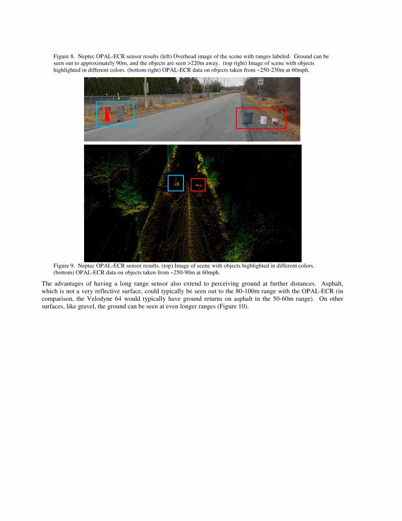
Figure 8. Neptec OPAL-ECR sensor results (left) Overhead image of the scene with ranges labeled. Ground can be

seen out to approximately 90m, and the objects are seen >220m away. (top right) Image of scene with objects

highlighted in different colors. (bottom right) OPAL-ECR data on objects taken from ~250-230m at 60mph.

Figure 9. Neptec OPAL-ECR sensor results. (top) Image of scene with objects highlighted in different colors.

(bottom) OPAL-ECR data on objects taken from ~250-90m at 60mph.

The advantages of having a long range sensor also extend to perceiving ground at further distances. Asphalt,

which is not a very reflective surface, could typically be seen out to the 80-100m range with the OPAL-ECR (in

comparison, the Velodyne 64 would typically have ground returns on asphalt in the 50-60m range). On other

surfaces, like gravel, the ground can be seen at even longer ranges (Figure 10).

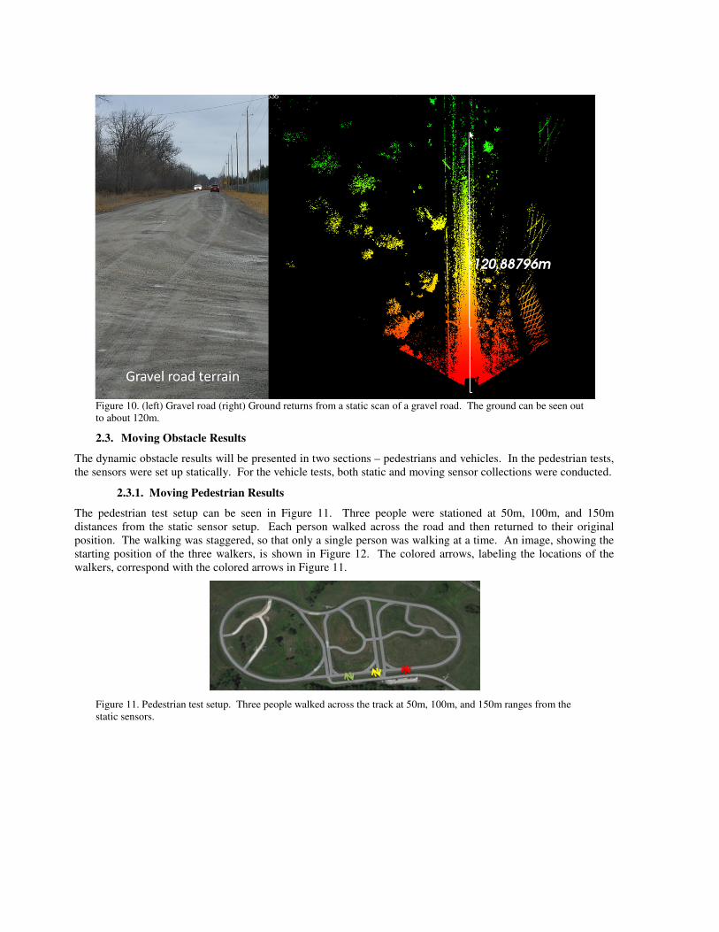
Figure 10. (left) Gravel road (right) Ground returns from a static scan of a gravel road. The ground can be seen out

to about 120m.

2.3. Moving Obstacle Results

The dynamic obstacle results will be presented in two sections – pedestrians and vehicles. In the pedestrian tests,

the sensors were set up statically. For the vehicle tests, both static and moving sensor collections were conducted.

2.3.1. Moving Pedestrian Results

The pedestrian test setup can be seen in Figure 11. Three people were stationed at 50m, 100m, and 150m

distances from the static sensor setup. Each person walked across the road and then returned to their original

position. The walking was staggered, so that only a single person was walking at a time. An image, showing the

starting position of the three walkers, is shown in Figure 12. The colored arrows, labeling the locations of the

walkers, correspond with the colored arrows in Figure 11.

Figure 11. Pedestrian test setup. Three people walked across the track at 50m, 100m, and 150m ranges from the

static sensors.

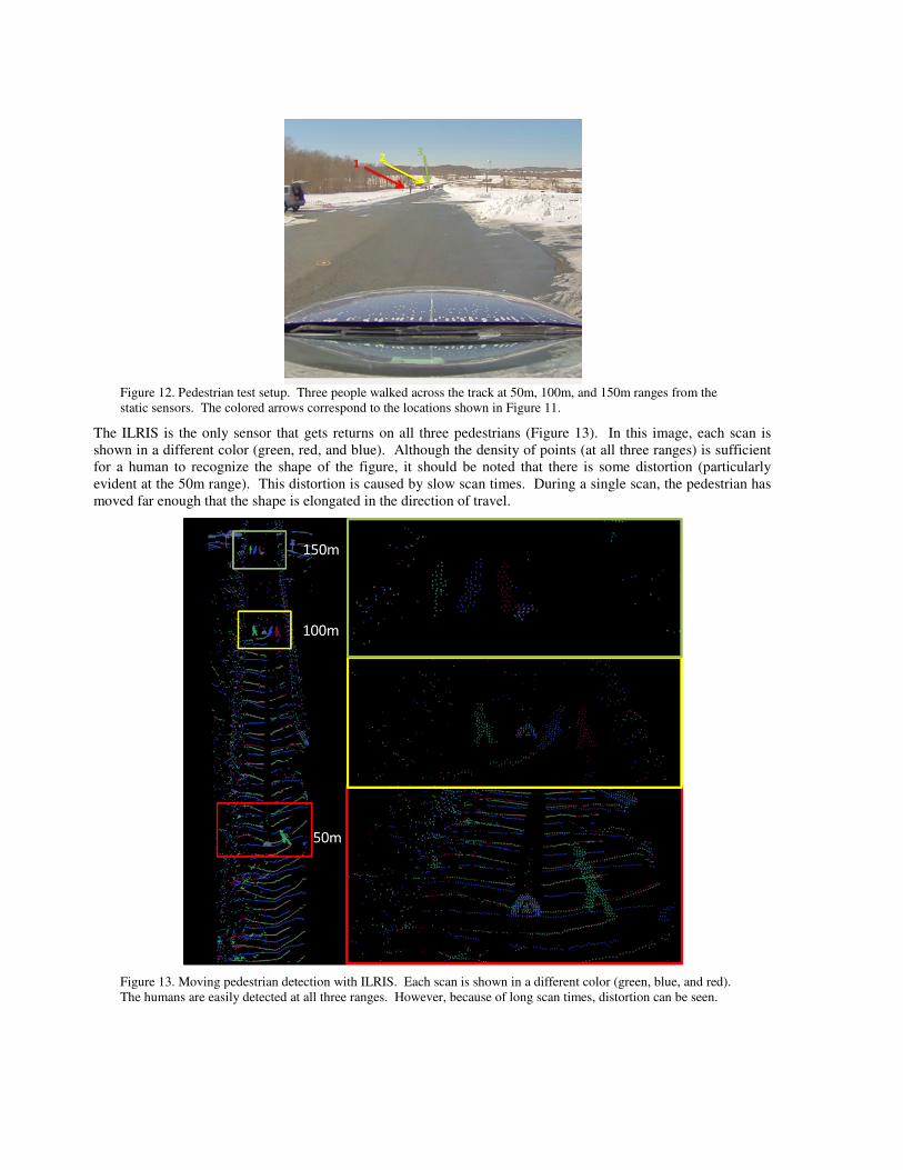
Figure 12. Pedestrian test setup. Three people walked across the track at 50m, 100m, and 150m ranges from the

static sensors. The colored arrows correspond to the locations shown in Figure 11.

The ILRIS is the only sensor that gets returns on all three pedestrians (Figure 13). In this image, each scan is

shown in a different color (green, red, and blue). Although the density of points (at all three ranges) is sufficient

for a human to recognize the shape of the figure, it should be noted that there is some distortion (particularly

evident at the 50m range). This distortion is caused by slow scan times. During a single scan, the pedestrian has

moved far enough that the shape is elongated in the direction of travel.

Figure 13. Moving pedestrian detection with ILRIS. Each scan is shown in a different color (green, blue, and red).

The humans are easily detected at all three ranges. However, because of long scan times, distortion can be seen.

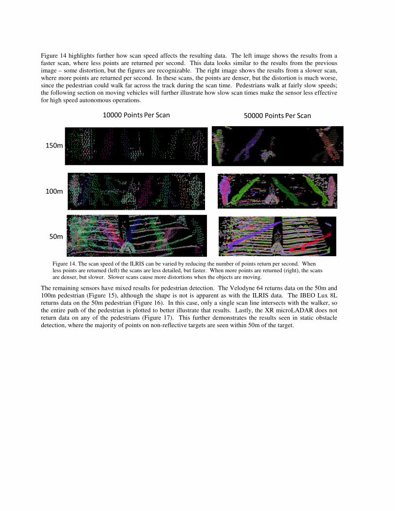
Figure 14 highlights further how scan speed affects the resulting data. The left image shows the results from a

faster scan, where less points are returned per second. This data looks similar to the results from the previous

image – some distortion, but the figures are recognizable. The right image shows the results from a slower scan,

where more points are returned per second. In these scans, the points are denser, but the distortion is much worse,

since the pedestrian could walk far across the track during the scan time. Pedestrians walk at fairly slow speeds;

the following section on moving vehicles will further illustrate how slow scan times make the sensor less effective

for high speed autonomous operations.

Figure 14. The scan speed of the ILRIS can be varied by reducing the number of points return per second. When

less points are returned (left) the scans are less detailed, but faster. When more points are returned (right), the scans

are denser, but slower. Slower scans cause more distortions when the objects are moving.

The remaining sensors have mixed results for pedestrian detection. The Velodyne 64 returns data on the 50m and

100m pedestrian (Figure 15), although the shape is not is apparent as with the ILRIS data. The IBEO Lux 8L

returns data on the 50m pedestrian (Figure 16). In this case, only a single scan line intersects with the walker, so

the entire path of the pedestrian is plotted to better illustrate that results. Lastly, the XR microLADAR does not

return data on any of the pedestrians (Figure 17). This further demonstrates the results seen in static obstacle

detection, where the majority of points on non-reflective targets are seen within 50m of the target.

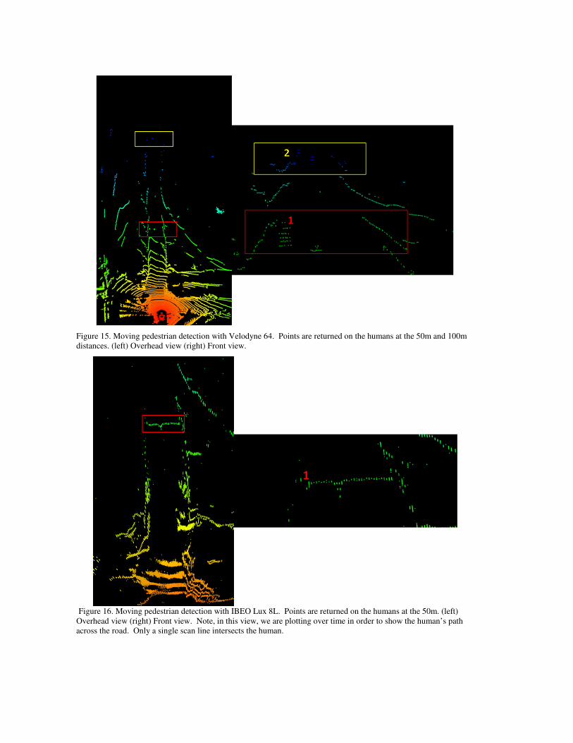
Figure 15. Moving pedestrian detection with Velodyne 64. Points are returned on the humans at the 50m and 100m

distances. (left) Overhead view (right) Front view.

Figure 16. Moving pedestrian detection with IBEO Lux 8L. Points are returned on the humans at the 50m. (left)

Overhead view (right) Front view. Note, in this view, we are plotting over time in order to show the human’s path

across the road. Only a single scan line intersects the human.

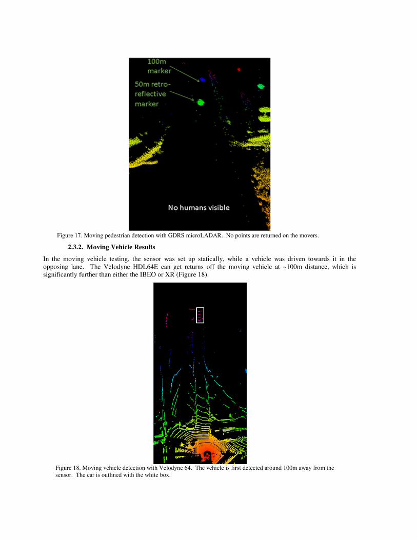
Figure 17. Moving pedestrian detection with GDRS microLADAR. No points are returned on the movers.

2.3.2. Moving Vehicle Results

In the moving vehicle testing, the sensor was set up statically, while a vehicle was driven towards it in the

opposing lane. The Velodyne HDL64E can get returns off the moving vehicle at ~100m distance, which is

significantly further than either the IBEO or XR (Figure 18).

Figure 18. Moving vehicle detection with Velodyne 64. The vehicle is first detected around 100m away from the

sensor. The car is outlined with the white box.

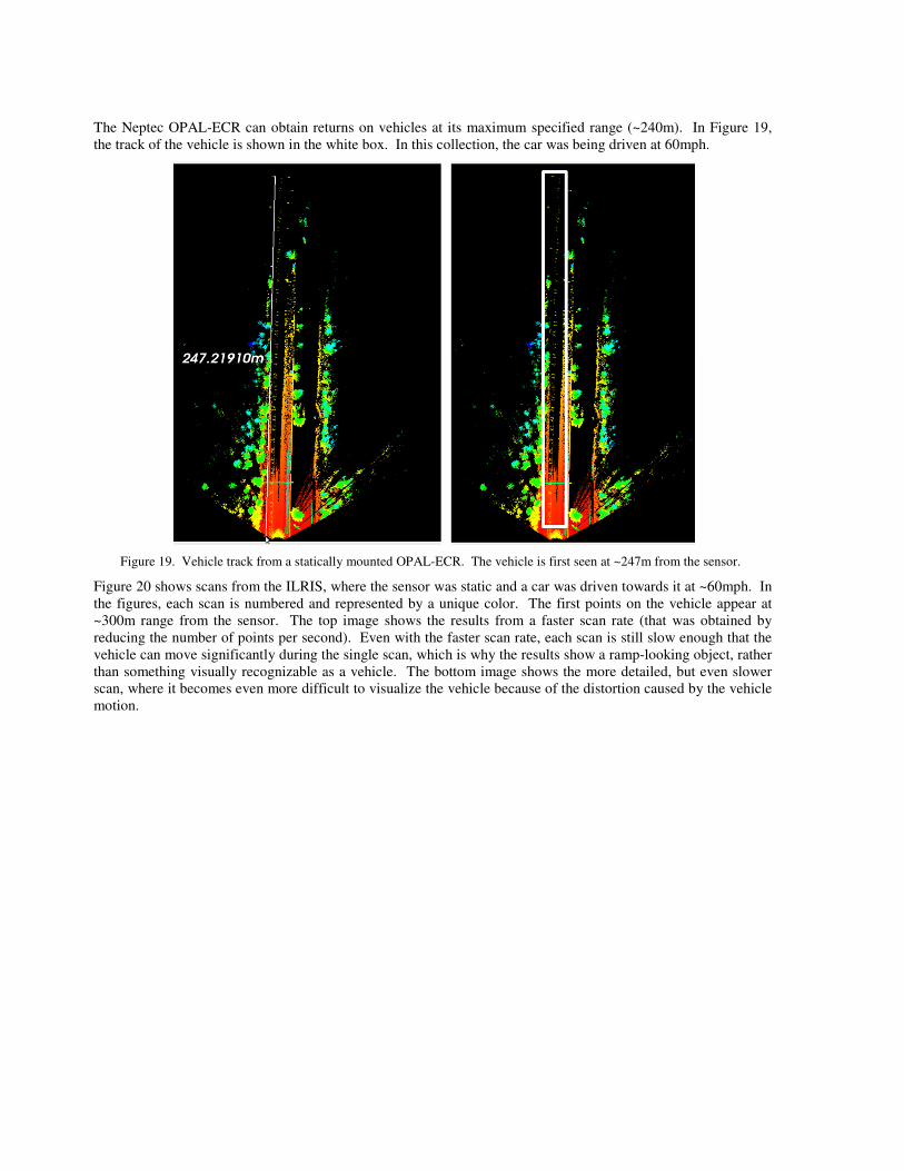
The Neptec OPAL-ECR can obtain returns on vehicles at its maximum specified range (~240m). In Figure 19,

the track of the vehicle is shown in the white box. In this collection, the car was being driven at 60mph.

Figure 19. Vehicle track from a statically mounted OPAL-ECR. The vehicle is first seen at ~247m from the sensor.

Figure 20 shows scans from the ILRIS, where the sensor was static and a car was driven towards it at ~60mph. In

the figures, each scan is numbered and represented by a unique color. The first points on the vehicle appear at

~300m range from the sensor. The top image shows the results from a faster scan rate (that was obtained by

reducing the number of points per second). Even with the faster scan rate, each scan is still slow enough that the

vehicle can move significantly during the single scan, which is why the results show a ramp-looking object, rather

than something visually recognizable as a vehicle. The bottom image shows the more detailed, but even slower

scan, where it becomes even more difficult to visualize the vehicle because of the distortion caused by the vehicle

motion.

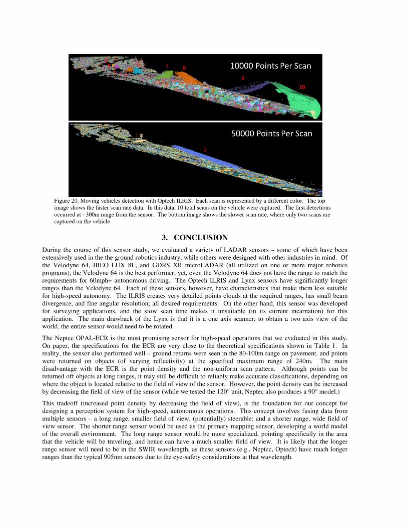
Figure 20. Moving vehicles detection with Optech ILRIS. Each scan is represented by a different color. The top

image shows the faster scan rate data. In this data, 10 total scans on the vehicle were captured. The first detections

occurred at ~300m range from the sensor. The bottom image shows the slower scan rate, where only two scans are

captured on the vehicle.

3. CONCLUSION

During the course of this sensor study, we evaluated a variety of LADAR sensors – some of which have been

extensively used in the the ground robotics industry, while others were designed with other industries in mind. Of

the Velodyne 64, IBEO LUX 8L, and GDRS XR microLADAR (all utilized on one or more major robotics

programs), the Velodyne 64 is the best performer; yet, even the Velodyne 64 does not have the range to match the

requirements for 60mph+ autonomous driving. The Optech ILRIS and Lynx sensors have significantly longer

ranges than the Velodyne 64. Each of these sensors, however, have characteristics that make them less suitable

for high-speed autonomy. The ILRIS creates very detailed points clouds at the required ranges, has small beam

divergence, and fine angular resolution; all desired requirements. On the other hand, this sensor was developed

for surveying applications, and the slow scan time makes it unsuitable (in its current incarnation) for this

application. The main drawback of the Lynx is that it is a one axis scanner; to obtain a two axis view of the

world, the entire sensor would need to be rotated.

The Neptec OPAL-ECR is the most promising sensor for high-speed operations that we evaluated in this study.

On paper, the specifications for the ECR are very close to the theoretical specifications shown in Table 1. In

reality, the sensor also performed well – ground returns were seen in the 80-100m range on pavement, and points

were returned on objects (of varying reflectivity) at the specified maximum range of 240m. The main

disadvantage with the ECR is the point density and the non-uniform scan pattern. Although points can be

returned off objects at long ranges, it may still be difficult to reliably make accurate classifications, depending on

where the object is located relative to the field of view of the sensor. However, the point density can be increased

by decreasing the field of view of the sensor (while we tested the 120° unit, Neptec also produces a 90° model.)

This tradeoff (increased point density by decreasing the field of view), is the foundation for our concept for

designing a perception system for high-speed, autonomous operations. This concept involves fusing data from

multiple sensors – a long range, smaller field of view, (potentially) steerable; and a shorter range, wide field of

view sensor. The shorter range sensor would be used as the primary mapping sensor, developing a world model

of the overall environment. The long range sensor would be more specialized, pointing specifically in the area

that the vehicle will be traveling, and hence can have a much smaller field of view. It is likely that the longer

range sensor will need to be in the SWIR wavelength, as these sensors (e.g., Neptec, Optech) have much longer

ranges than the typical 905nm sensors due to the eye-safety considerations at that wavelength.

REFERENCES

[1] Schneider, A., LaCelle, Z., Lacaze, A., Murphy, K., Del Giorno, M., Close, R., “Sensor study for high speed

autonomous operations,” Proc. SPIE 9494 (2015)