Returns on Real Estate Investment in theCase-Shiller Composite Cities

By Joseph Fairchild

Submitted to the graduate degree program in Economics and the GraduateFaculty of the University of Kansas in partial fulfillment of the requirementsfor the degree of Master of Arts.

Professor Shu Wu

Professor Ted Juhl

Professor Ronald Caldwell

Date Defended: 4/3/2012

The Thesis Committee for Joseph Fairchild certifies that this isthe approved version of the following thesis:

Returns on Real Estate Investment in the Case-Shiller

Composite Cities

By Joseph Fairchild

Professor Shu Wu

Date Approved: 4/3/2012

ii

Abstract

In this paper we estimate the housing services dividend in eight major U.S.cities using data from the U.S. Census. We then construct quarterly timeseries of housing investment total returns using the Case-Shiller house priceindex and Bureau of Labor Statistics rent index data. Using the resultingtotal return data we estimate the optimal allocation of household wealthto the housing asset. We find that in each city two equilibrium portfoliosobtain, one for renters and one for homeowners. Moreover, we find that theallocation results are critically dependent upon the inclusion of dividends inthe analysis. If we optimize using only capital gains on housing investment,optimal investment in the housing asset goes to zero in all but two cities.

iii

1 Introduction

In this paper we study returns to real estate investment across several large

U.S. cities. In particular, we will study price and dividend variation across

8 of the 10 U.S. cities (metropolitan areas) that comprise the Case-Shiller

10-city composite house price index. These 8 cities represent 35% of the

housing value in the U.S. (Standard and Poors, 2008.) The Case-Shiller

index, published monthly by Standard & Poors and Fiserv, has become the

most watched housing variable in the U.S. We will also examine the Federal

Housing Finance Agency (FHFA) house price index across the same cities.

The Case-Shiller index is considered to be more representative of the state

of the housing market than FHFA because the latter is composed only of

conforming mortgages. For example, in recent years in cities such as San

Francisco and San Diego, many homes transacted above the conforming limit.

Thus, the data across cities are right truncated to varying degrees. However,

during the real estate bubble, which was largely driven by sub-prime finance

(e.g., Piazzesi, et al., 2011), the GSE’s Fannie Mae and Freddie Mac were

not purchasing much of the lower strata mortgages either. Consequently,

the FHFA index is left truncated as well. There are other features that

differentiate the two indices (OFHEO, 2008). However, we will see that for

our purposes the differences are not consequential.

We are ultimately interested in the portion of household wealth that should

be optimally allocated to the housing asset. To that end, we must estimate

the total return on house i, Rit+1:

Rit+1 =

P it+1 + Di

t+1

P it

Both price, P it , and dividends, Di

t, are difficult to estimate. Houses are highly

illiquid and transact infrequently, and so P it is only occasionally observed.

Moreover, the dividend component, Dit, is not directly observed.

1

1.1 Prices

In practice it is house prices that are most often estimated. A common

specification for house prices is the following (Hwang, et al., 2010):

pit = θpt + Qi

t + eit = θpt + βX i

t + eit

Where pit is the log of the observed transaction price of house i at time t, pt

is the log of the representative house (e.g., for the entire U.S., or perhaps a

local market that contains house i), Qit is log quality of house i, and X i

t are

measurement variables associated with Qit (i.e., hedonic variables). If house

i transacts at times t1 and t2 and quality does not change, then the house

price appreciation rate over the period [t1, t2] is:

pit2− pi

t1= θ(pt2 − pt1) + β(X i

t2−X i

t1) + (ei

t2− ei

t1) = θ(pt2 − pt1) + ηi

t2

Thus, house price appreciation (HPA) for the i-th house can be decomposed

into an aggregate component and an idiosyncratic component. This is the

basis for constant quality repeat sales indices such as FHFA and Case-Shiller.

In such indices it is assumed the quality of housing services consumed between

the times of the sales pair transactions was constant. It is difficult to believe

that quality is constant for a single house, if for no other reason depreciation

and improvements. Moreover, when aggregating over houses, the distribution

of quality is changing over time (as new homes are added to the housing

stock) and across space (at any time, quality varies over geography). It is

also possible the market’s valuation of the same services provided by a house

changes over time, due to changing preferences.

It is likely that all repeat sales house price indices are biased estimates of

unobserved house price returns because of sample selection bias (Gatzlaff

and Haurin, 1997). In particular, only houses that are sold are included in

the sample used to estimate HPA. Assume the unobservable HPA process for

2

the i-th house evolves in accordance with the following:

dhit = θi(µi − hi

t)dt + σidWt

The unobserved price at time t2 is:

P i,ut2 = P i,u

t1 eR t2

t1dhi

s

For this illustration, let us assume that the highest offer price at t2 equals

P i,ut2 . House i transacts at time t2 when the offer price exceeds the seller’s

reservation price. The time t2 prices in the data (such as those used for

this study), P it2, are transacted prices. Thus, there is an upward bias in the

time t2 transacted prices. Moreover, the same self selection occurs at time

t1. Thus, repeat sales indices suffer from double selectivity (Gatzlaff and

Haurin, 1997).

1.2 Dividends

Theoretically, we can relate prices and dividends for house i in the following

expression:

P it =

∑Tτ=0 M i

t+τDit+τ + M i

T LiT

Where M it+τ is the discounted marginal utility of agent/household i, and Li

T

is the value of the land at T . The salvage value, M iT Li

T , presupposes that at

time T the house is fully depreciated.

For now, the important point is that the expression above depends upon the

quantity of services, i.e., dividends, which we cannot observe, constant or

otherwise. In this paper we will use hedonic methods to estimate dividends

(Goodman, 2005 and Davis, et al., 2008).

3

1.3 Measurement of Returns

The housing dividend is paid continuously and is perishable. If one purchases

more house than they can actually consume, some of the housing services

provided are lost. If an agent purchases too much house as an ”investment”,

and consumes less than 100% of the dividend, what is their return on the

housing asset? They are actually foregoing the opportunity to consume other

goods and services in favor of the lost housing services. It seems that this

feature particularly exposes homeowners to over investing in housing.

In this paper all return calculations implicitly assume the housing dividend

is entirely consumed. To the extent that this is not the case, it would seem

that total returns to housing would be overstated. Housing overinvestment

does appear to be a problem in the United States, at least during the bub-

ble when resources were overinvested in housing. Are agents behaving irra-

tionally? One explanation could be that agents purchase more house than

they can consume based upon the view that on net (after considering the lost

consumption on wasted dividends) they will make a sufficient risk-adjusted

return to compensate. This is not borne out by the price return data. Are

agents simply making bad forecasts? Alternatively, agents are receiving util-

ity from what appears to be overinvestment that is not captured by the

standard specification.

4

2 Data

2.1 Data Sources

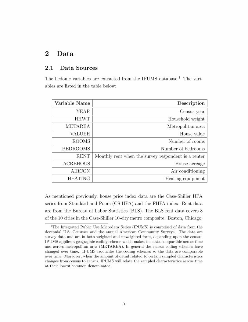
The hedonic variables are extracted from the IPUMS database.1 The vari-

ables are listed in the table below:

Variable Name Description

YEAR Census year

HHWT Household weight

METAREA Metropolitan area

VALUEH House value

ROOMS Number of rooms

BEDROOMS Number of bedrooms

RENT Monthly rent when the survey respondent is a renter

ACREHOUS House acreage

AIRCON Air conditioning

HEATING Heating equipment

As mentioned previously, house price index data are the Case-Shiller HPA

series from Standard and Poors (CS HPA) and the FHFA index. Rent data

are from the Bureau of Labor Statistics (BLS). The BLS rent data covers 8

of the 10 cities in the Case-Shiller 10-city metro composite: Boston, Chicago,

1The Integrated Public Use Microdata Series (IPUMS) is comprised of data from thedecennial U.S. Censuses and the annual American Community Surveys. The data aresurvey data and are in both weighted and unweighted form, depending upon the census.IPUMS applies a geographic coding scheme which makes the data comparable across timeand across metropolitan area (METAREA). In general the census coding schemes havechanged over time. IPUMS reconciles the coding schemes so the data are comparableover time. Moreover, when the amount of detail related to certain sampled characteristicschanges from census to census, IPUMS will relate the sampled characteristics across timeat their lowest common denominator.

5

Denver, Los Angeles, Miami, New York, San Diego, and San Francisco.2

2.2 Data Discussion

We assume the hedonic variables that determine the dividend value of house

i at time t are number of rooms (ROOMS), number of bedrooms (BED-

ROOMS), location/city (METAREA), house acreage (ACREHOUS), air con-

ditioning (AIRCON), and heating equipment (HEATING). Number of rooms

contains number of bedrooms. It would seem that number of rooms alone

may be sufficient. However, researchers (e.g., Goodman, 2005) typically use

both bedrooms and rooms as separate regressors. We tested both specifica-

tions; number of bedrooms is significant.

2.3 Data Preparation

The ROOMS and BEDROOMS variables were grouped into categories. We

experimented with using the actual value (e.g., there are houses with 29

rooms) as well as the categories approach. In both cases the SAS procedure

treats the variables as categorical.3 The results from the two methods are

qualitatively indistinguishable. The results reported are based upon the cat-

egories approach. The variables ACREHOUS, AIRCON, and HEATING are

binary.

2This is why we study 8 of the 10 cities in the Case-Shiller composite.3Statistical Analysis Software, SAS Institute, Inc.

6

3 Model Specification and Estimation

3.1 Rent Regressions

Using the RENT data, we estimate the following cross-sectional regression

for each of the 8 cities in the sample:

RENT i,mt = β0,m

t +∑R

r=1 βr,mt 1{r} +

∑Bb=1 βb,m

t 1{b} + βah,mt 1{ah}

+ βac,mt 1{ac} + βh,m

t 1{h} + εi,mt

For each city m, we fix year t = 1980.4

The indicator corresponds to the appropriate categorical variables. The vari-

able superscripts correspond to METAREA (m), ROOMS (r), BEDROOMS

(b), ACREHOUS (ah), AIRCON (ac), and HEATING (h). For example, if

observation i has heating but no air conditioning, sits on less than one acre,

number of rooms and bedrooms categories equal X and Y , respectively, and

is in city W , then 1{m=W}, 1{r=X}, 1{b=Y }, 1{ah} = 1, 1{ac} = 1, and 1{h} = 0.

The values of the βjt are estimates of the contribution to RENT i

t correspond-

ing to the values of the hedonic variables.

We estimated a semi-log specification of the above model as well. The semi-

log specification is often encountered in the hedonic house price model liter-

ature. However, the results were not qualitatively different.

3.2 Housing Dividend Estimation

The rent regression results are applied to each house i to estimate the divi-

dend time series, Di,mt :

4AIRCON and HEATING are only available in the 1980 survey, so we fix t = 1980.We also estimated a model for t=1980, ..., t=2009, without the AIRCON and HEATINGregressors.

7

Di,mt = β0,m

t +∑R

r=1 βr,mt 1{i,r} +

∑Bb=1 βb,m

t 1{i,b} + βah,mt 1{i,ah}

+ βac,mt 1{i,ac} + βh,m

t 1{i,h}

The i subscript in the indicator notation is meant to signify the appropriate

value for house i. Thus, the regression maps the observable hedonic variables

for each house in the survey to its dividend.

4 Return Estimation Results

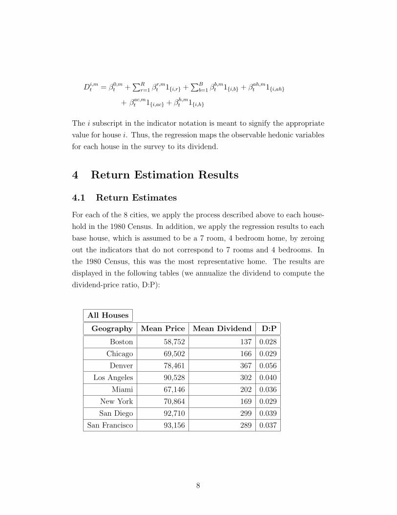
4.1 Return Estimates

For each of the 8 cities, we apply the process described above to each house-

hold in the 1980 Census. In addition, we apply the regression results to each

base house, which is assumed to be a 7 room, 4 bedroom home, by zeroing

out the indicators that do not correspond to 7 rooms and 4 bedrooms. In

the 1980 Census, this was the most representative home. The results are

displayed in the following tables (we annualize the dividend to compute the

dividend-price ratio, D:P):

All Houses

Geography Mean Price Mean Dividend D:P

Boston 58,752 137 0.028

Chicago 69,502 166 0.029

Denver 78,461 367 0.056

Los Angeles 90,528 302 0.040

Miami 67,146 202 0.036

New York 70,864 169 0.029

San Diego 92,710 299 0.039

San Francisco 93,156 289 0.037

8

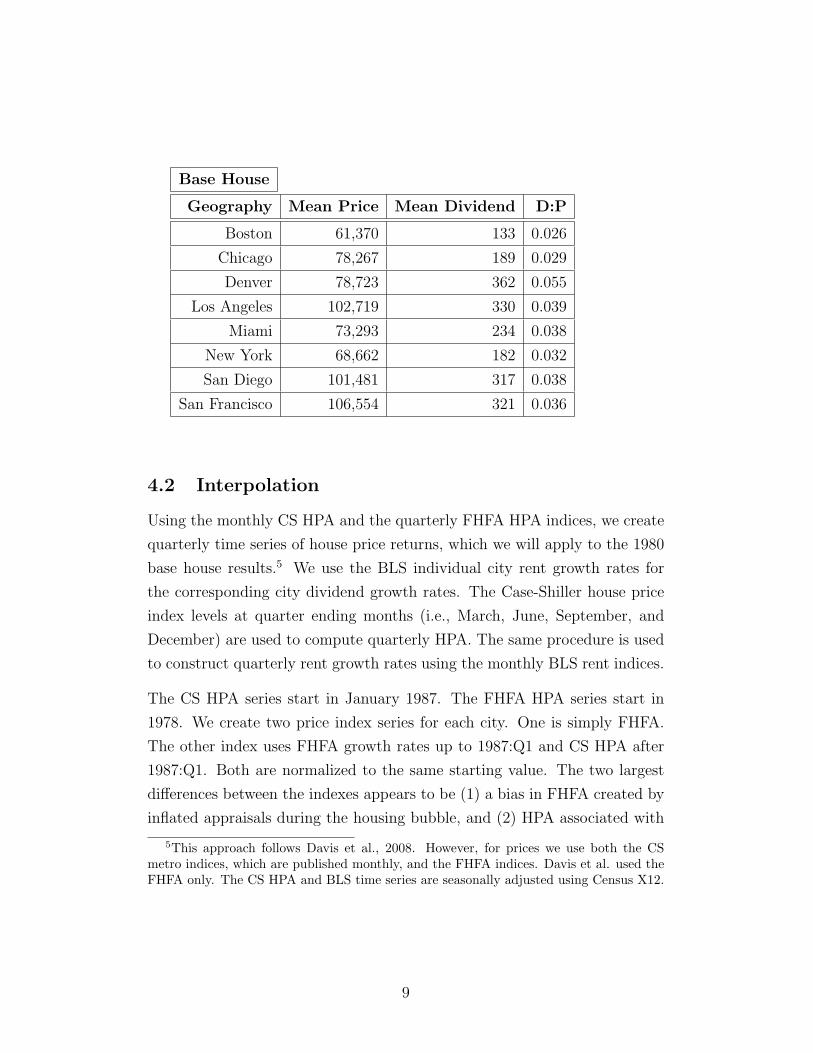
Base House

Geography Mean Price Mean Dividend D:P

Boston 61,370 133 0.026

Chicago 78,267 189 0.029

Denver 78,723 362 0.055

Los Angeles 102,719 330 0.039

Miami 73,293 234 0.038

New York 68,662 182 0.032

San Diego 101,481 317 0.038

San Francisco 106,554 321 0.036

4.2 Interpolation

Using the monthly CS HPA and the quarterly FHFA HPA indices, we create

quarterly time series of house price returns, which we will apply to the 1980

base house results.5 We use the BLS individual city rent growth rates for

the corresponding city dividend growth rates. The Case-Shiller house price

index levels at quarter ending months (i.e., March, June, September, and

December) are used to compute quarterly HPA. The same procedure is used

to construct quarterly rent growth rates using the monthly BLS rent indices.

The CS HPA series start in January 1987. The FHFA HPA series start in

1978. We create two price index series for each city. One is simply FHFA.

The other index uses FHFA growth rates up to 1987:Q1 and CS HPA after

1987:Q1. Both are normalized to the same starting value. The two largest

differences between the indexes appears to be (1) a bias in FHFA created by

inflated appraisals during the housing bubble, and (2) HPA associated with

5This approach follows Davis et al., 2008. However, for prices we use both the CSmetro indices, which are published monthly, and the FHFA indices. Davis et al. used theFHFA only. The CS HPA and BLS time series are seasonally adjusted using Census X12.

9

houses not financed by the GSE’s Fannie Mae and Freddie Mac (OFHEO,

2008).

The period from 1978 through 1987 contains much less of these two features.

Firstly, inflated appraisals were associated with increasing rates of home

equity extraction during the boom phase of the bubble (e.g., Greenspan and

Kennedy, 2007 and Silva, 2005). Secondly, the bubble that pushed higher

strata houses beyond the conforming limits began in 2002. The lower strata

homes not financed by the GSE’s were sub-prime financed homes, which

began to occur during the boom phase of the bubble (LeCour-Little, et al.,

2008). As a result, over the 1978 to 1987 periods the two indices would be

fairly comparable.

The factors that differentiate FHFA and CS HPA do become important in

later years. The first differentiating factor becomes significant around the

beginning of the bubble in 2002. In addition, the distribution of home values

have become increasingly skewed in the direction of higher-valued homes over

the last 40 years. We will see later that higher-valued homes appear to be

less attractive than median-valued homes as investment assets. By using the

two indexes we can compare these effects across cities.

5 Analysis of Returns

We shall examine housing return statistics against the S&P 500 total return

as an initial benchmark.6

5.1 Mean and Volatility of Quarterly Returns

The interpolation process produces 8 time series of 134 quarterly returns.

The annualized mean returns, mean excess returns, and return volatilities

6The S&P 500 total return data are obtained from Robert Shiller’s website,www.econ.yale.edu/∼shiller/data.htm.

10

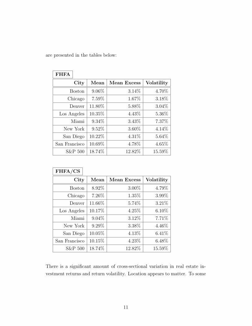
are presented in the tables below:

FHFA

City Mean Mean Excess Volatility

Boston 9.06% 3.14% 4.70%

Chicago 7.59% 1.67% 3.18%

Denver 11.80% 5.88% 3.04%

Los Angeles 10.35% 4.43% 5.36%

Miami 9.34% 3.43% 7.37%

New York 9.52% 3.60% 4.14%

San Diego 10.22% 4.31% 5.64%

San Francisco 10.69% 4.78% 4.65%

S&P 500 18.74% 12.82% 15.59%

FHFA/CS

City Mean Mean Excess Volatility

Boston 8.92% 3.00% 4.79%

Chicago 7.26% 1.35% 3.99%

Denver 11.66% 5.74% 3.21%

Los Angeles 10.17% 4.25% 6.10%

Miami 9.04% 3.12% 7.71%

New York 9.29% 3.38% 4.46%

San Diego 10.05% 4.13% 6.41%

San Francisco 10.15% 4.23% 6.48%

S&P 500 18.74% 12.82% 15.59%

There is a significant amount of cross-sectional variation in real estate in-

vestment returns and return volatility. Location appears to matter. To some

11

extent, the results above are predicted by housing market models that in-

clude land supply elasticity (Gyourko et al. 2006, 2008). This work predicts

the emergence of ”superstar cities”, which are characterized as highly desir-

able and highly supply inelastic. High income families sort into these cities,

a process which bids up prices. The results above are in accord with the

superstar city theory and the Wharton Residential Land Use Regulatory In-

dex (WRLURI) (Gyourko et al., 2007). According to the WRLURI, Denver,

San Francisco, and San Diego have highly inelastic land supply. Chicago has

elastic land supply. Los Angeles and New York are both relatively inelastic

and should be roughly comparable according to the WRLURI, which is the

case. Both New York and Boston experienced rent controls over much of

the sample period. It is possible that land supply inelasticity in New York

and Boston results in significant land premiums.7 However, the presence of

rent controls would depress dividends. Depressed dividends combined with

significant land premiums result in lower returns than would otherwise be

observed. Miami is not included in the WRLURI, however this area is cat-

egorized as a highly land elastic city in Gyourko et al., 2006. According to

this research, Denver is highly attractive but is less supply inelastic than Los

Angeles, San Diego, and San Francisco. (Denver is not bordered by an ocean

and therefore has less physical land restrictions.) Finally, it is interesting

that when high value properties are added (i.e., the FHFA/CS index), in

every city mean returns declined and return volatility increased.

6 Analysis of Housing as an Investment Class

In this section we want to ask the following two questions:

(1) Should investment in the housing asset exceed zero?

7Such a land premium is predicted by the model in Gyourko et al., 2006.

12

(2) If agents should invest in the housing asset, how much investment is

optimal?

We will provide answers in the following subsections under assumptions sim-

ilar to those that underlie the Capital Asset Pricing Model.

6.1 Investment in a Primary Residence

We assume that risky financial asset returns are normally distributed (prices

are lognormally distributed). Let the expected return and volatility of any

risky portfolio be denoted µp and σp, respectively. We define the efficient

frontier as the portion of the boundary of the set {µp, σp} that contains the

largest µp for each element σp (Merton, 1972). Investors are risk averse and

prefer more to less. Finally, assume that investors can borrow and lend at the

risk free rate (i.e., a risk free asset is available). It follows that in equilibrium

all investors will hold a linear combination of the market portfolio and the

risk free asset (Lintner, 1965). In particular, denote the expected return

and volatility of the market portfolio as µM and σM , respectively. Denote

the return on the risk free asset as Rf . In equilibrium, the i-th investor’s

portfolio will have an expected return and volatility as follows:

E[Rip] = ωiRf + (1− ωi)µM

σip = (1− ωi)σM

Where ωi varies over investor and is determined by the i-th investor’s pref-

erences. The set formed over all values of ωi is the capital market line.

When risk free lending and borrowing is possible, a linear combination of the

risk free asset and the tangency portfolio of the efficient frontier dominates all

other portfolios along the efficient frontier. In (µp, σp) - space, the tangency

portfolio is the portfolio on the efficient frontier that is tangent to a line

13

intersecting the risk free rate. This is the capital market line in (µp, σp) -

space, and points along it satisfy the following equation:

µp = Rf +µM −Rf

σM

σp

Within this context we can rephrase question (1) from above as follows: If

we add the housing asset to the investment opportunity set, is the efficient

frontier expanded outward? If yes, then a linear combination of the risk

free asset and the new tangency portfolio will dominate the case without the

housing asset. That is to say, in (µp, σp) - space, the new capital market line

will be above the previous capital market line.

Assume that housing investment is non-negative, i.e., investors cannot short

the housing asset. Assume housing returns are normally distributed. Let µjh

and σhj denote the expected return and return volatility of the housing asset

in city j, respectively. In addition, denote the correlation between the return

on the market portfolio and the city j housing asset as ρM,hj . We assume in

this setup that one can own a housing asset in city j only by living in city j.

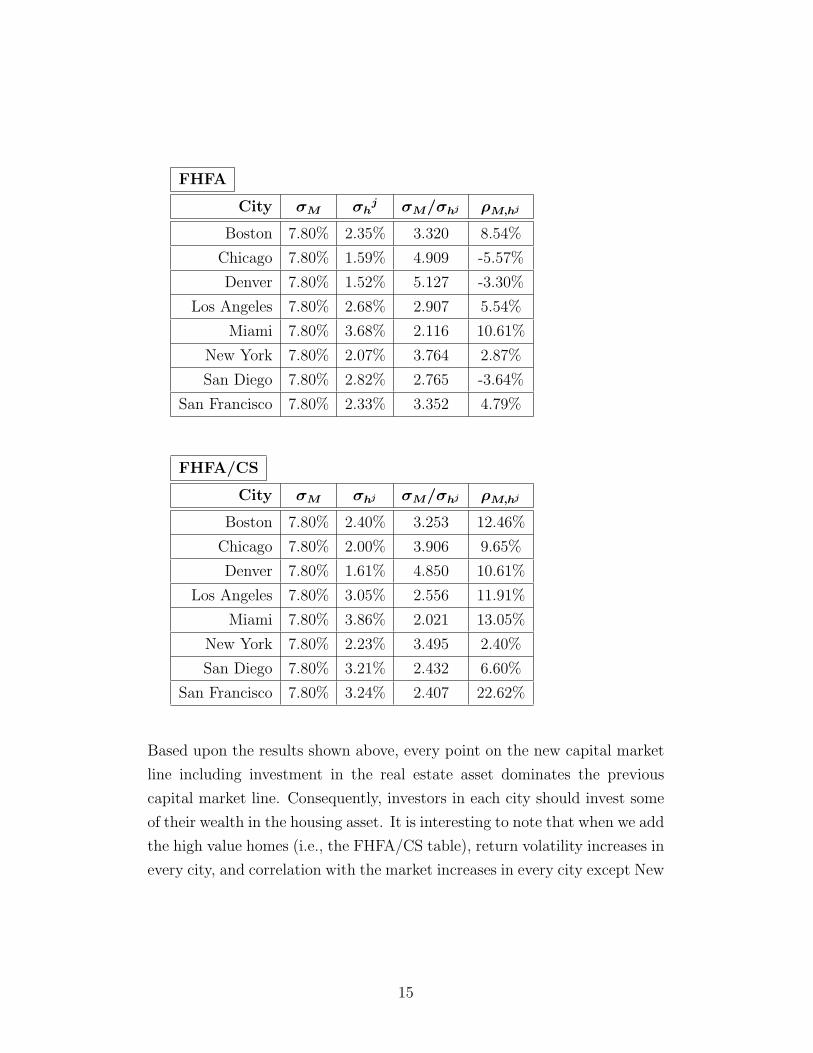
If ρM,hj < σM/σhj , then the efficient frontier will expand beyond the current

capital market line (Cox, et al., 2000). (The proof of this result is in the

Appendix.) The following tables display the result of this test (values below

are not annualized):

14

FHFA

City σM σhj σM/σhj ρM,hj

Boston 7.80% 2.35% 3.320 8.54%

Chicago 7.80% 1.59% 4.909 -5.57%

Denver 7.80% 1.52% 5.127 -3.30%

Los Angeles 7.80% 2.68% 2.907 5.54%

Miami 7.80% 3.68% 2.116 10.61%

New York 7.80% 2.07% 3.764 2.87%

San Diego 7.80% 2.82% 2.765 -3.64%

San Francisco 7.80% 2.33% 3.352 4.79%

FHFA/CS

City σM σhj σM/σhj ρM,hj

Boston 7.80% 2.40% 3.253 12.46%

Chicago 7.80% 2.00% 3.906 9.65%

Denver 7.80% 1.61% 4.850 10.61%

Los Angeles 7.80% 3.05% 2.556 11.91%

Miami 7.80% 3.86% 2.021 13.05%

New York 7.80% 2.23% 3.495 2.40%

San Diego 7.80% 3.21% 2.432 6.60%

San Francisco 7.80% 3.24% 2.407 22.62%

Based upon the results shown above, every point on the new capital market

line including investment in the real estate asset dominates the previous

capital market line. Consequently, investors in each city should invest some

of their wealth in the housing asset. It is interesting to note that when we add

the high value homes (i.e., the FHFA/CS table), return volatility increases in

every city, and correlation with the market increases in every city except New

15

York. This latter finding has been discovered by other researchers (Anderson

and Beracha, 2010). This finding is also consistent with the superstar city

research. As in Gyourko, et al., 2006, superstar city house price behavior is

a consequence of a sorting process in which wealthier households sort into

and bid up prices in the superstar cities (such as San Francisco, the authors’

prototypical superstar city). Wealthier households are more exposed to the

capital markets (2007 SCF and 2009 SCFP), and therefore, house prices in

such cities would be more correlated with the capital markets (Anderson and

Beracha, 2010).

6.2 Optimal Investment in the Housing Asset

Now we are in a position to examine question (2) above, i.e., given that

investors should allocate wealth to the housing asset, what is the optimal

allocation? To answer this question, first we assume that an investor in city

j can allocate some of their wealth to the housing asset in city j only. Thus,

there will be a new tangency portfolio for each city. In principle, we can

determine the expanded portfolio for each city (Luenberger, 1998). Note

that for any feasible portfolio p we can compute the Sharpe ratio:

µp

σp

Where µp and σp are the mean and standard deviation of the excess returns

of portfolio p, respectively.

The tangency portfolio is the efficient portfolio with the highest Sharpe ratio.

Thus, for each city we must find the portfolio weights αk such that:

max{αk}

∑nk=1 αkµk√∑n

k,m=1 σk,mαkαm

Where there are k risky assets, including the housing asset, σk,m is the return

16

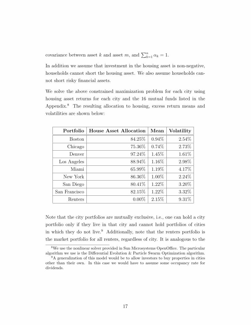
covariance between asset k and asset m, and∑n

k=1 αk = 1.

In addition we assume that investment in the housing asset is non-negative,

households cannot short the housing asset. We also assume households can-

not short risky financial assets.

We solve the above constrained maximization problem for each city using

housing asset returns for each city and the 16 mutual funds listed in the

Appendix.8 The resulting allocation to housing, excess return means and

volatilities are shown below:

Portfolio House Asset Allocation Mean Volatility

Boston 84.25% 0.94% 2.54%

Chicago 75.36% 0.74% 2.73%

Denver 97.24% 1.45% 1.61%

Los Angeles 88.94% 1.16% 2.98%

Miami 65.99% 1.19% 4.17%

New York 86.36% 1.00% 2.24%

San Diego 80.41% 1.22% 3.20%

San Francisco 82.15% 1.22% 3.32%

Renters 0.00% 2.15% 9.31%

Note that the city portfolios are mutually exclusive, i.e., one can hold a city

portfolio only if they live in that city and cannot hold portfolios of cities

in which they do not live.9 Additionally, note that the renters portfolio is

the market portfolio for all renters, regardless of city. It is analogous to the

8We use the nonlinear solver provided in Sun Microsystems OpenOffice. The particularalgorithm we use is the Differential Evolution & Particle Swarm Optimization algorithm.

9A generalization of this model would be to allow investors to buy properties in citiesother than their own. In this case we would have to assume some occupancy rate fordividends.

17

market portfolio, which is different from the S&P 500, which we used as the

market portfolio proxy above. The asset allocation of the renters portfolio

is different than the S&P 500 (neither is the market portfolio). We include

it here so that we can compare the renters portfolio to the homeowners

portfolios over the same investment opportunity set (i.e., the aforementioned

16 funds).

The model predicts that there are two equilibrium market portfolios for each

city: the renters portfolio without the housing asset, and a city-specific mar-

ket portfolio which includes some proportion of the housing asset. In each

city equilibrium, all renter households hold a linear combination of the risk

free asset and the renters portfolio, and all homeowner households hold a lin-

ear combination of the risk free asset and the city market portfolio. Moreover,

note that in each city equilibrium all homeowner households are exposed to

the housing asset in the same proportion. However, the amount of allocation

to housing varies considerably across cities. This is something that should

be researched further, i.e., does the allocation to the housing asset vary over

geography?

We have already established that some allocation to the housing asset results

in an investment opportunity set that dominates the portfolio without city-

specific housing investment opportunities. Nonetheless, it is surprising how

much wealth should be allocated to the housing asset. The reason is because

the housing asset is essentially a bond with zero credit risk. That is to say,

the dividend payments occur with probability one. The resale value of the

housing asset has significant volatility, however it has almost no correlation

with the rest of the market, which provides valuable diversification benefits.

This result does not occur if we don’t include dividends. If we were to (in-

correctly) compute the optimal allocation using price returns only, every city

except for Boston (35.7%) and Denver (83.9%) would result in zero allocation

to the housing asset. In all other cities, everyone would rent and hold the

18

renters portfolio. This would be inconsistent with reality. As pointed out

earlier, the analysis in this paper assumes that the entire dividend (housing

services) is consumed. The price-return only analysis reveals that if home-

buyers purchase too much house ”as an investment”, they are likely making

a financial mistake.

6.3 Numerical Example

The housing asset has a very high unit price, i.e., in order to receive the

dividends the investor must purchase the entire house. In our model each

homebuyer is buying the 4-bedroom, 7-room base house in their city. Recall

that we have assumed that investors can borrow and lend at the risk free

rate. Let us consider the San Diego market. If the investor decides to be

a homebuyer, the optimal allocation to housing is 80%. Assume the base

house has a current market price of $80,000 and that the investor currently

has $30,000 fully invested in the renters portfolio. Assume that in order to

borrow at the risk free rate, the borrower must make a down payment of

$10,000 on the house. Once the homebuyer has decided to purchase a house,

their optimal allocation including housing requires the following rebalancing:

• Borrow $70,000 at the risk free rate.

• Using the borrowed $70,000 and $10,000 down payment, purchase the

house for $80,000.

• Rebalance the remaining $20,000 according to the optimal San Diego

homeowner city portfolio allocation.

After rebalancing, this investor is on the San Diego capital market line, and

is a net borrower. That is to say, they are borrowing at the risk free rate

and are to the right of the San Diego tangency portfolio in (µp, σp) - space.

19

Specifically, their optimal allocation is net short risk free bonds. Any position

that contains long treasuries would not be optimal. This is an interesting

result, since most homebuyers are net borrowers. In particular, no homebuyer

that is a net borrower should be long treasuries in any amount. It should

be pointed out that homebuyers cannot borrow at the risk free rate, which

complicates the analysis; a potential topic for further study.

7 Conclusions and Areas for Further Study

7.1 Findings/Conclusions

• In order to properly measure returns to housing investment, we must

estimate the housing services dividend.

• Housing investment expands the investment opportunity set.

• Housing investment is included in the new tangency portfolio.

• Housing expands the city CML because it is a bond with zero credit risk

and has very low correlation with risky financial market assets. This

result depends critically upon the assumption that the entire housing

services dividend is consumed every period.

• Optimal housing investment varies over geography.

• The typical rule of thumb of buying more housing than can be con-

sumed ”as an investment” leads to overinvestment in housing.

• Optimal housing portfolios that are net short borrowing should contain

zero long treasury positions.

20

7.2 Areas for Further Study

• Study the problem with a dynamic allocation model. In particular,

house price returns are highly persistent. Such an approach would

significantly mitigate the re-sale risk of the housing asset.10

• Study housing investment allocations across metropolitan areas.

• Although the housing asset allocations seem large, they are not incon-

sistent with informal (anecdotal) evidence. A more rigorous study of

homeowner portfolio allocations should be done if data are available.

(PSID or Survey of Consumer Finances data, for example, or a survey.)

• Relax the assumption homebuyers can borrow at the risk free rate.

The primary current coupon (the rate borrowers pay) floats at a small

spread to the constant maturity mortgage rate, which is the par rate

from the TBA MBS market. This rate in turn floats at a narrow spread

above the same duration treasury yields.

• Investors that have reached a satiation point with respect to housing

should not invest more in their primary residence, which would violate

the assumption underlying this analysis, i.e., that the dividend is fully

consumed each period. Direct allocation to housing is needed for re-

balancing, which is difficult. Publicly traded REITs and REIT-based

ETFs do not provide direct exposure to the housing asset. A new class

of private equity funds have recently begun to emerge which provide

direct exposure to real estate. Do these new instruments represent

efficient allocation opportunities?

10That is, house price returns are forecastable, and so sales can be timed which willreduce price risk.

21

8 Bibliography

[1] S&P/Case-Shiller Home Price Indices, Index Methodology, Standard &

Poors, March, 2008.

[2] Tim Landvoigt, Monika Piazzesi, and Martin Schneider, The Housing

Market(s) of San Diego, Working Paper, 2011., 41:3-23.

[3] Revisiting the Differnces between the OFHEO and S&P/Case-Shiller

House Price Indexes: New Explanations, Office of Federal Housing Enter-

prise Oversight, 2008.

[4] Min Hwang and John Quigley, Housing Price Dynamics in Time and

Space: Predictability, Liquidity and Investor Returns, Journal of Real Estate

Finance and Economics, 2010, 41:3-23.

[5] Dean H. Gatzlaff and Donald R. Haurin, Sample Selection Bias and

Repeat-Sales Index Estimates, Journal of Real Estate Finance and Eco-

nomics, 1997, 14:33-50.

[6] Jack Goodman, Constant Quality Rent Indexes for Affordable Housing,

Joint Center for Housing Studies, Harvard University, June 2005.

[7] Morris Davis, Andreas Lehnert, and Robert Martin, The Rent-Price Ratio

for the Aggregate Stock of Owner-Occupied Housing, Review of Income and

Wealth, 2008, vol.54(2):279-284.

[8] Joseph Gyourko, Edward Glaeser, and Albert Saiz, Housing Supply and

Housing Bubbles, Journal of Urban Economics, 2008, Vol. 64, no. 3:198-217.

[9] Joseph Gyourko, Christopher J. Mayer, and Todd Sinai, Superstar Cities,

Wharton Real Estate Center, Working Paper, June 2006.

[10] Joseph Gyourko, Albert Saiz, and Anita A. Summers, A New Measure

of Local Regulatory Environment for Housing Markets, Urban Studies, 2008,

22

Vol. 45, no. 3:693-729.

[11] Karl E. Case and Robert J. Shiller, Forecasting Prices and Excess Re-

turns in the Housing Market, AREUEA Journal, 1990, Vol. 18, No. 3:253-

273.

[12] Robert C. Merton, On Estimating the Expected Return on the Market,

Journal of Financial Economics, 8, 1980, 323-361.

[13] Alan Greenspan and James Kennedy, Sources and Uses of Equity Ex-

tracted from Homes, Finance and Economics Discussion Series, Federal Re-

serve Board, 2007.

[14] Javier Silva, A House of Cards: Refinancing the American Dream, Bor-

rowing to Make Ends Meet Briefing Paper #3, Demos, 2005.

[15] Major Coleman, Michael LaCour-Little, and Kerry Vandell, Subprime

Lending and the Housing Bubble: Tail Wags Dog?, Journal of Housing Eco-

nomics, 17(4), 2008, 631-673.

[16] John Lintner, The Valuation of Risky Assets and the Selection of Risky

Investments in Stock Portfolios and Capital Budgets, Review of Economics

and Statistics, 47, 1965, 1337.

[17] Robert C. Merton, An Analytic Derivation of the Efficient Portfolio

Frontier, The Journal of Financial and Quantitative Analysis, 7(4), 1972,

1851-1872.

[18] Samuel H. Cox, Joseph R. Fairchild, and Hal W. Pedersen, Economic

Aspects of Securitization of Risk, ASTIN Bulletin, 30(1), 2000, 157-193.

[19] Survey of Consumer Finances (2007 SCF) and Survey of Consumer Fi-

nances Panel (2009 SCFP), Federal Reserve Board.

[20] Christopher W. Anderson and Eli Beracha, Home-Price Sensitivity to

Capital Market Factors: Analysis of Zip Code Level Data, Journal of Real

23

Estate Research 32, No. 2, 2010, 161-185.

[21] David G. Luenberger, Investment Science, Oxford University Press, 1998.

24

9 Appendix

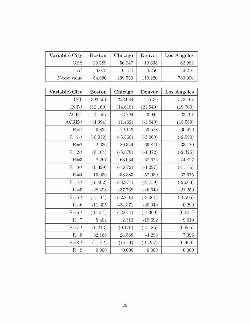
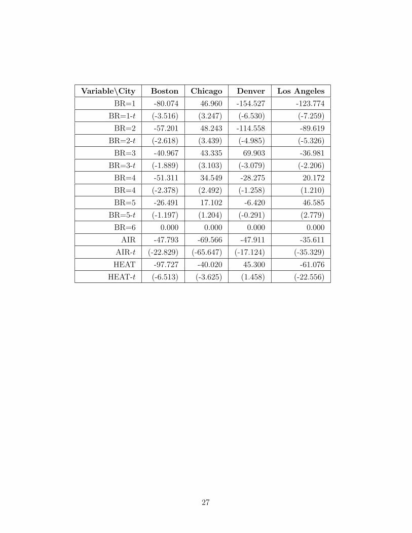
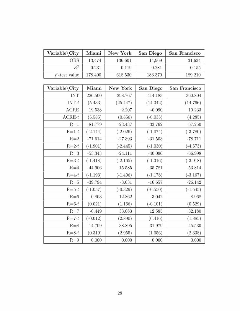
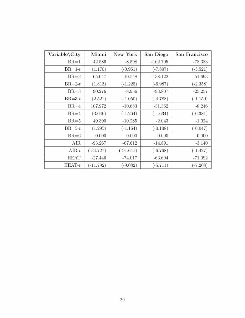
9.1 Estimation Results

The table below summarizes the rent regression results using the 1980 U.S.

Census data.

OBS=number of observations, INT=intercept, ACRE=acreage indicator value

at zero, R=number of rooms, BR=number of bedrooms, AIR=air condition-

ing indicator value at zero, HEAT=heating indicator value at zero. Values

of t-statistics are denoted, e.g., BR=1-t, and values in the table are in paren-

thesis.

25

Variable\City Boston Chicago Denver Los Angeles

OBS 20,589 56,047 10,638 82,962

R2 0.073 0.134 0.250 0.216

F -test value 54.990 299.550 110.220 780.900

Variable\City Boston Chicago Denver Los Angeles

INT 302.501 258.084 417.36 373.167

INT-t (12.169) (14.618) (21.549) (19.760)

ACRE 21.507 3.794 -3.944 23.791

ACRE-t (4.394) (1.462) (-1.040) (18.589)

R=1 -0.835 -79.143 -53.528 -30.429

R=1-t (-0.032) (-5.569) (-3.060) (-2.090)

R=2 2.636 -80.344 -69.811 -33.170

R=2-t (0.104) (-5.878) (-4.372) (-2.326)

R=3 8.267 -63.034 -67.675 -44.827

R=3-t (0.329) (-4.672) (-4.297) (-3.156)

R=4 -10.036 -53.383 -57.939 -37.675

R=4-t (-0.402) (-3.977) (-3.759) (-2.663)

R=5 -28.498 -37.768 -46.640 -21.250

R=5-t (-1.144) (-2.819) (-3.061) (-1.505)

R=6 -11.305 -34.871 -20.040 0.299

R=6-t (-0.454) (-2.611) (-1.300) (0.021)

R=7 5.404 2.313 -19.692 9.619

R=7-t (0.213) (0.170) (-1.185) (0.665)

R=8 32.169 24.568 -4.293 7.396

R=8-t (1.172) (1.614) (-0.257) (0.466)

R=9 0.000 0.000 0.000 0.000

26

Variable\City Boston Chicago Denver Los Angeles

BR=1 -80.074 46.960 -154.527 -123.774

BR=1-t (-3.516) (3.247) (-6.530) (-7.259)

BR=2 -57.201 48.243 -114.558 -89.619

BR=2-t (-2.618) (3.439) (-4.985) (-5.326)

BR=3 -40.967 43.335 69.903 -36.981

BR=3-t (-1.889) (3.103) (-3.079) (-2.206)

BR=4 -51.311 34.549 -28.275 20.172

BR=4 (-2.378) (2.492) (-1.258) (1.210)

BR=5 -26.491 17.102 -6.420 46.585

BR=5-t (-1.197) (1.204) (-0.291) (2.779)

BR=6 0.000 0.000 0.000 0.000

AIR -47.793 -69.566 -47.911 -35.611

AIR-t (-22.829) (-65.647) (-17.124) (-35.329)

HEAT -97.727 -40.020 45.300 -61.076

HEAT-t (-6.513) (-3.625) (1.458) (-22.556)

27

Variable\City Miami New York San Diego San Francisco

OBS 13,474 136,601 14,969 31,634

R2 0.231 0.119 0.281 0.155

F -test value 178.400 618.530 183.370 189.210

Variable\City Miami New York San Diego San Francisco

INT 226.500 298.767 414.183 360.804

INT-t (5.433) (25.447) (14.342) (14.766)

ACRE 19.538 2.207 -0.090 10.233

ACRE-t (5.585) (0.856) (-0.035) (4.285)

R=1 -81.779 -23.437 -33.762 -67.250

R=1-t (-2.144) (-2.026) (-1.074) (-3.780)

R=2 -71.614 -27.393 -31.503 -78.711

R=2-t (-1.901) (-2.445) (-1.030) (-4.573)

R=3 -53.343 -24.111 -40.096 -66.998

R=3-t (-1.418) (-2.165) (-1.316) (-3.918)

R=4 -44.906 -15.585 -35.781 -53.814

R=4-t (-1.193) (-1.406) (-1.178) (-3.167)

R=5 -39.794 -3.631 -16.657 -26.142

R=5-t (-1.057) (-0.329) (-0.550) (-1.545)

R=6 0.803 12.862 -3.042 8.968

R=6-t (0.021) (1.166) (-0.101) (0.529)

R=7 -0.449 33.083 12.585 32.180

R=7-t (-0.012) (2.890) (0.416) (1.885)

R=8 14.709 38.895 31.979 45.530

R=8-t (0.319) (2.955) (1.056) (2.338)

R=9 0.000 0.000 0.000 0.000

28

Variable\City Miami New York San Diego San Francisco

BR=1 42.586 -8.598 -162.705 -78.383

BR=1-t (1.170) (-0.951) (-7.807) (-3.521)

BR=2 65.047 -10.548 -138.122 -51.693

BR=2-t (1.813) (-1.225) (-6.987) (-2.358)

BR=3 90.276 -8.956 -93.807 -25.257

BR=3-t (2.521) (-1.050) (-4.788) (-1.159)

BR=4 107.972 -10.683 -31.362 -8.246

BR=4 (3.046) (-1.264) (-1.634) (-0.381)

BR=5 49.390 -10.285 -2.043 -1.024

BR=5-t (1.295) (-1.164) (-0.108) (-0.047)

BR=6 0.000 0.000 0.000 0.000

AIR -93.267 -67.612 -14.891 -3.140

AIR-t (-34.727) (-91.641) (-6.768) (-1.427)

HEAT -27.446 -74.017 -63.604 -71.092

HEAT-t (-11.792) (-9.082) (-5.711) (-7.208)

29

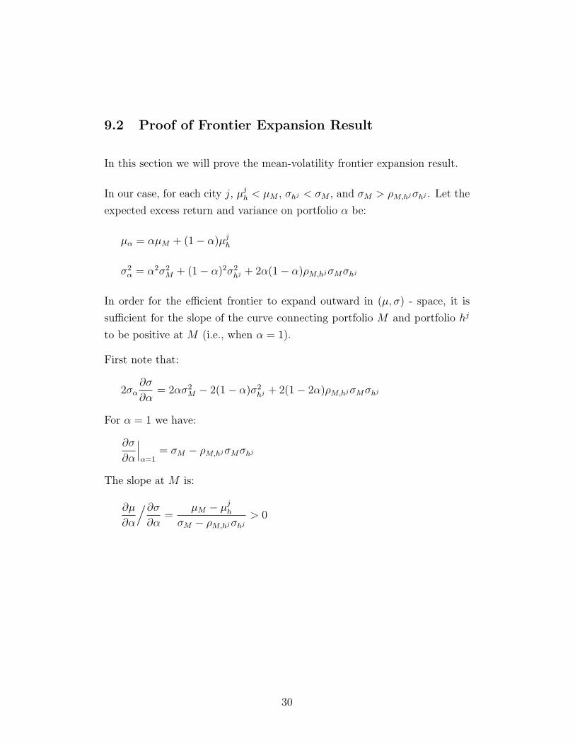
9.2 Proof of Frontier Expansion Result

In this section we will prove the mean-volatility frontier expansion result.

In our case, for each city j, µjh < µM , σhj < σM , and σM > ρM,hjσhj . Let the

expected excess return and variance on portfolio α be:

µα = αµM + (1− α)µjh

σ2α = α2σ2

M + (1− α)2σ2hj + 2α(1− α)ρM,hjσMσhj

In order for the efficient frontier to expand outward in (µ, σ) - space, it is

sufficient for the slope of the curve connecting portfolio M and portfolio hj

to be positive at M (i.e., when α = 1).

First note that:

2σα∂σ

∂α= 2ασ2

M − 2(1− α)σ2hj + 2(1− 2α)ρM,hjσMσhj

For α = 1 we have:

∂σ

∂α

∣∣∣α=1

= σM − ρM,hjσMσhj

The slope at M is:

∂µ

∂α

/∂σ

∂α=

µM − µjh

σM − ρM,hjσhj

> 0

30

9.3 Funds in Portfolio Allocation Optimization

• Putnam Voyager

• Fidelity Magellan

• Putnam Convertible Securities Fund

• Fidelity Capital and Income Fund

• Fidelity Intermediate Municipal Bond Fund

• Fidelity Contra Fund

• Fidelity Equity Income Fund

• Fidelity Fund

• Vanguard Intermediate Term Municipal

• Vanguard Investment Grade Bond

• Vanguard Long Term Municipal

• Vanguard Morgan Growth Fund

• Dreyfus Mid-Cap Fund

• Dreyfus Research Growth Fund

• Oppenheimer AMT-free Municipal

• Oppenheimer Capital Income Fund

31

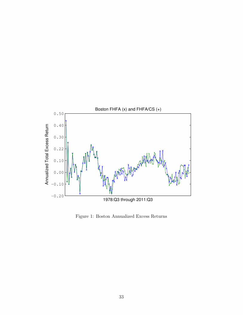
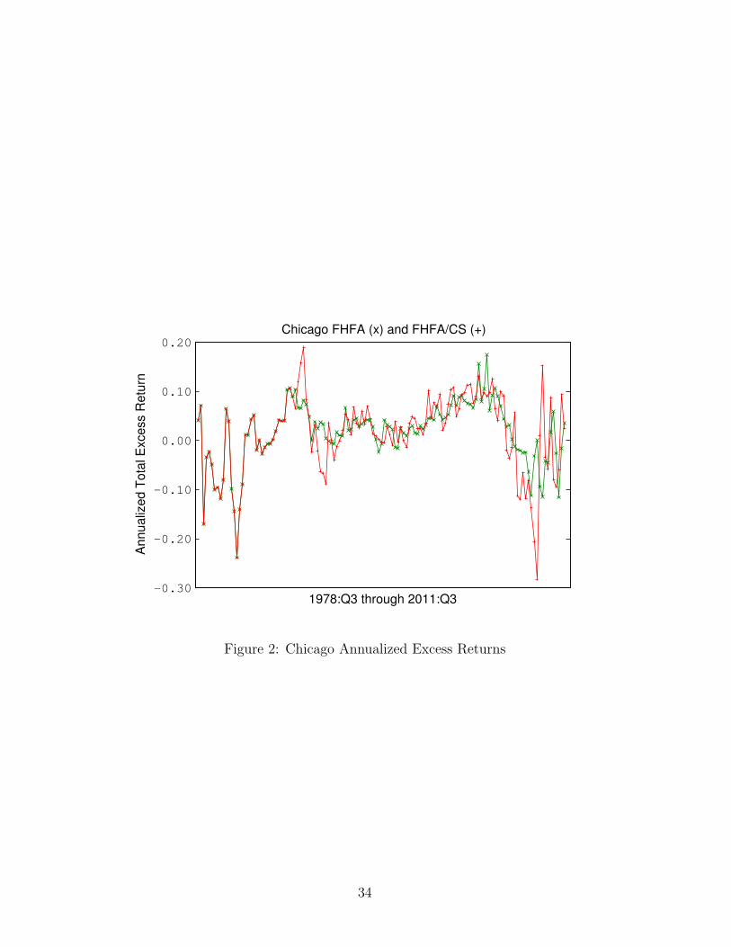
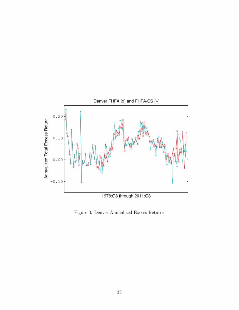
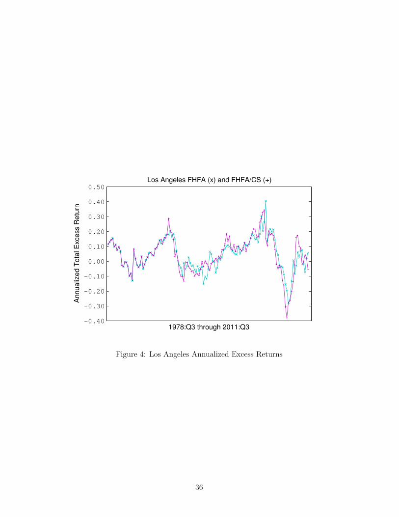
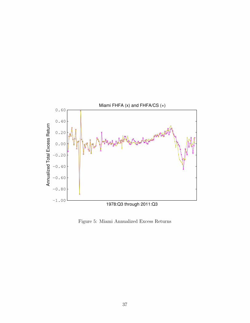
9.4 Interpolated Housing Returns by City

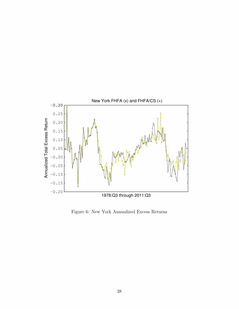
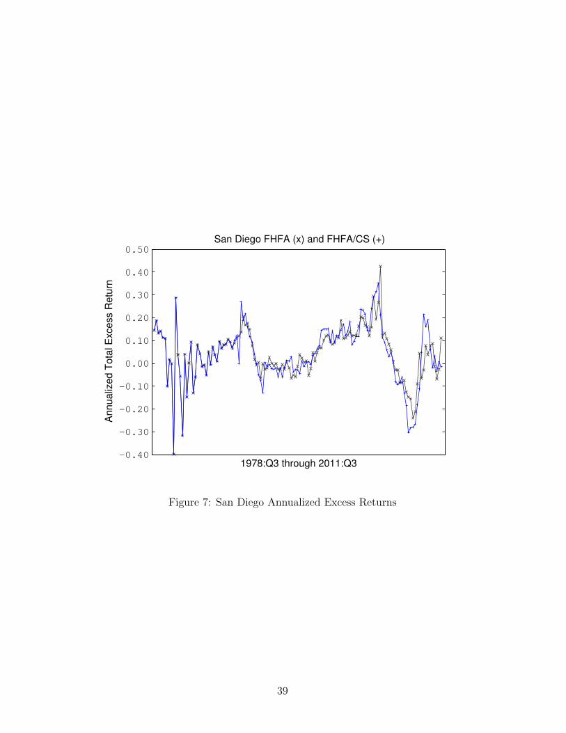
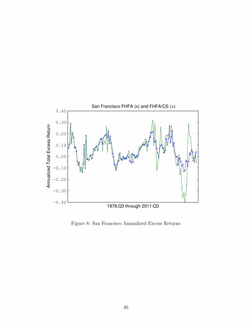
The following graphs present the FHFA and FHFA/CS interpolated total re-

turn series. Note that the two series coincide from 1978:Q3 through 1987:Q1.

32

−0.20

−0.10

0.00

0.10

0.22

0.30

0.40

0.50

Boston FHFA (x) and FHFA/CS (+)

1978:Q3 through 2011:Q3

Annualiz

ed T

ota

l E

xcess R

etu

rn

Figure 1: Boston Annualized Excess Returns

33

−0.30

−0.20

−0.10

0.00

0.10

0.20

1978:Q3 through 2011:Q3

An

nu

aliz

ed

To

tal E

xce

ss R

etu

rn

Chicago FHFA (x) and FHFA/CS (+)

Figure 2: Chicago Annualized Excess Returns

34

−0.10

0.00

0.10

0.20

Denver FHFA (x) and FHFA/CS (+)

1978:Q3 through 2011:Q3

Annualiz

ed T

ota

l E

xcess R

etu

rn

Figure 3: Denver Annualized Excess Returns

35

−0.40

−0.30

−0.20

−0.10

0.00

0.10

0.20

0.30

0.40

0.50

1978:Q3 through 2011:Q3

An

nu

aliz

ed

To

tal E

xce

ss R

etu

rn

Los Angeles FHFA (x) and FHFA/CS (+)

Figure 4: Los Angeles Annualized Excess Returns

36

−1.00

−0.80

−0.60

−0.40

−0.20

0.00

0.20

0.40

0.60

Miami FHFA (x) and FHFA/CS (+)

1978:Q3 through 2011:Q3

Annualiz

ed T

ota

l E

xcess R

etu

rn

Figure 5: Miami Annualized Excess Returns

37

−0.20

−0.15

−0.10

−0.05

−0.00

0.05

0.10

0.15

0.20

0.25

0.30−0.20

New York FHFA (x) and FHFA/CS (+)

1978:Q3 through 2011:Q3

Annualiz

ed T

ota

l E

xcess R

etu

rn

Figure 6: New York Annualized Excess Returns

38

−0.40

−0.30

−0.20

−0.10

0.00

0.10

0.20

0.30

0.40

0.50

San Diego FHFA (x) and FHFA/CS (+)

1978:Q3 through 2011:Q3

Annualiz

ed T

ota

l E

xcess R

etu

rn

Figure 7: San Diego Annualized Excess Returns

39

−0.40

−0.30

−0.20

−0.10

0.00

0.10

0.20

0.30

0.40

San Francisco FHFA (x) and FHFA/CS (+)

1978:Q3 through 2011:Q3

Annualiz

ed T

ota

l E

xcess R

etu

rn

Figure 8: San Francisco Annualized Excess Returns

40