Revenue Sharing, Competitive Balance, and

Incentives in Major League Baseball

How MLB Revenue Sharing Made the Yankees Better

William Ryan Colby

Advisors: Frank Westhoff and Andrew Zimbalist

Spring 2011

Submitted to the Department of Economics at Amherst College in partial fulfillment of the

requirements for the degree of Bachelor of Arts with Honors

i

Abstract

Many contend that demand for sporting events is directly related to the

uncertainty of the outcome of the contest. By the 1990‟s many professional sports

leagues, specifically Major League Baseball, began worrying that outcomes were

becoming too deterministic and that increases in competitive balance were necessary to

maintain and increase demand. In 1996, Major League Baseball introduced its first

system of comprehensive revenue sharing with the goal of creating more competitive

balance in the league.

In this work, I develop a theoretical model of a profit maximizing sports league.

This model demonstrates that the popular two-team case frequently used to examine the

effects of revenue sharing on competitive balance is inadequate in the n-team case. I

demonstrate that with three or more teams, revenue sharing can affect competitive

balance. Following this analysis, I argue that the marginal tax rates created by MLB‟s

revenue sharing systems have actually worsened balance in the league. Although the

most recent sharing system begins to realign incentives, it still risks “turning a „good‟

imbalance into a „bad‟ one” by subsidizing poorly managed teams at the expense of well

run teams.

I construct an empirical model of revenue generation that can serve as a basis for

a new system that will realign incentives and reduce the risk of subsidizing poor

performance. Having constructed a measure of market strength, I show that the incentive

structures created by MLB revenue sharing had the anticipated negative effects on

competitive balance.

ii

Acknowledgments

It is customary to acknowledge your project advisors at this point, but the amount

of help, insight, and dedication to this paper that my two advisors showed was far from

customary. This project is a testament to their patience, helpfulness, tireless energy, and

support. Professors Frank Westhoff and Andrew Zimbalist have been fantastic

throughout; in the good, the bad, and the ugly. For this I will always be grateful.

I would also like to thank the entire Economics Department for their guidance

over the last four years. One document, even one as long as this, cannot begin to

encompass all that I will take away from my career in economics at Amherst. I would

also like to thank Jeanne Reinle for not only making the project run smoothly, but also

for her energy and enthusiasm that often brighten the Economics Computer Lab.

I also owe a debt of gratitude to the Tampa Bay Rays organization for which I had

the good fortune to work last summer. My time in St. Petersburg taught me much about

the way that sports teams ought to be run and about the experiences of a small market

team in the AL East. I would like to specifically thank Michael Kalt, Melanie Lenz, Bill

Walsh, and Robbie Artz for providing me with the experience of a lifetime.

I should also thank all of my friends for helping me to stay focused on the project.

Specifically, I should thank Reid Fitzgerald and Alex Fraser for their daily humor and

support. In addition, I must thank my coach and “informal” advisor, Nick Nichols for

years of patience and dedication.

Perhaps most importantly, I must thank my family. My mother for her unending

support and encouragement; my father for teaching me all the baseball teams by division

by the time I was four years old and instilling a lifelong love of the game that has led to

this project; and my sister for frequently reminding me of all the other things in the world

that I need to care about in addition to this project.

iii

Table of Contents

Abstract ............................................................................................................................................. i

Acknowledgments............................................................................................................................ ii

1 Introduction ............................................................................................................................... 1

2 Literature Review...................................................................................................................... 2

2.1 The Theoretical Justifications for Balance ......................................................................... 3

2.2 Empirical Evidence on the Effect of Balance .................................................................... 5

2.3 Can Revenue Sharing Affect Balance? .............................................................................. 7

3 A Theoretical Model of Revenue Sharing .............................................................................. 11

3.1 The Two-Team Case ........................................................................................................ 13

3.2 The Three Team Case ...................................................................................................... 15

4 Major League Baseball‟s Attempts to Promote Balance ........................................................ 19

4.1 Luxury Taxes ................................................................................................................... 20

4.2 Revenue Sharing .............................................................................................................. 23

5 Empirical Data Analysis ......................................................................................................... 33

5.1 Data .................................................................................................................................. 33

5.2 Choice of Model ............................................................................................................... 34

5.3 Specification of the Model ................................................................................................ 34

5.4 Results .............................................................................................................................. 38

5.5 A New Sharing System .................................................................................................... 42

5.6 The Effect of Revenue Sharing on Balance in MLB ....................................................... 46

6 Conclusion .............................................................................................................................. 48

REFERENCES .............................................................................................................................. 49

1

1 Introduction

Andrew Zimbalist reports that “the revenue disparity between the richest and

poorest teams was around $30 million in 1989, but by 1999 it was $163 million.”

(Zimbalist 2003, 46) Many factors contribute to this growth in revenue disparity

including the proliferation of new stadiums, the growing importance of the business

community, and the growing value of local broadcasting rights. In particular, broadcast

deals had been relatively small until George Steinbrenner and the Yankees signed a

contract with Madison Square Garden in 1989 worth $493 million over 12 years.

(Zimbalist 2003, 12) James Quirk and Rodney Fort also demonstrate the growing

inequality as they write that “the 1996 statistics for MLB show that average media

income per team was $25.2 million, but the range was from a low of $15.1 million

(Milwaukee) to a high of $69.8 million (New York Yankees).” (Quirk and Fort 1999, 36)

Prolonged revenue disparities such as have developed in MLB since the late

1980‟s have led to attempts to reduce the growing inequalities in revenue and on-field

performance. Unfortunately, MLB has implemented solutions in collective bargaining

since 1996 that proved largely ineffective and may have contributed to the problems.

In this paper, I develop a theoretical model of revenue sharing that shows that

revenue sharing (1) will not affect balance in a two-team league and (2) can affect

balance in an n-team league. I then use marginal tax rates to show that the revenue

sharing structures implemented by MLB likely decrease competitive balance. Following

this analysis, I develop an empirical model of revenue generation in MLB that identifies

market strength. I use this model to show that

2

(1) MLB CBAs have not differentiated between “good” imbalance and “bad”

imbalance leading to the subsidization of poor performance

(2) MLB teams acted upon the perverse incentive schemes in the 1996 and 2002

revenue sharing systems and exacerbated the competitive imbalance in MLB

(3) The 2006 CBA may begin to move balance back to the competitive, pre-

sharing, level, but player salaries are “sticky” due to the preponderance of

multi-year deals making this analysis difficult.

I begin in section 2 with a review of the literature; section 3 introduces the theoretical

model; section 4 discusses revenue sharing in MLB; section 5 models revenue generation

and analyzes the effect of the CBAs on competitive balance; and section 6 concludes.

2 Literature Review

The uniqueness of the sports industry has been apparent as long as economists

have studied it. In 1956, Simon Rottenberg noted that “the nature of the industry is such

that competitors must be of approximately equal „size‟ if any are to be successful.”

(Rottenberg 1956, 242) To this end, some leagues have implemented revenue sharing

plans among teams.1 Despite a general consensus about the importance of competitive

balance, the literature is less unified on the effects of revenue sharing plans.

Consistent with the literature, I isolate three distinct types of “uncertainty of

outcome.” These are: match uncertainty, seasonal uncertainty, and championship

uncertainty (Szymanski 2003, 1155). Match uncertainty refers to the uncertainty of an

individual game, seasonal to an individual season, and championship to many seasons.

Each author constructs an argument using one or more of these types of uncertainty.

1 Of the big four American sports leagues, only the NBA does not share local revenue, but that will likely change with the new Collective Bargaining Agreement due in summer 2011.

3

2.1 The Theoretical Justifications for Balance

The relationship between competitive balance and interest in professional team

sports is complicated. The popularity of sporting events relies on the uncertainty of the

outcome of the contest, a feature that Walter C. Neale calls the “Louis-Schmelling

Paradox.” He writes that “the greater the economic collusion and the more the sporting

competition the greater the profits.” (Neale 1964, 2) Neale contends that contests require

uncertain outcomes to generate profits.

On the other hand, some contend that balance is either not important or that some

degree of imbalance may enhance interest and profits. Michael R. Canes argues that

If team income reflects the value of its performance to spectators, and if

the demand for winning teams differs among areas, some owners will have

a greater incentive than others to build a strong team. In such a case, a

policy aimed at equalizing team strengths would transfer quality from

areas where winning is more valued to areas where it is less valued.

(Canes 1974, 82)

Canes argues that if fans in New York City value a quality baseball team more than fans

in Kansas City, then the Yankees should have a stronger team than the Royals. Many

economists agree with this contention, but recognize that a certain amount of balance

must exist beyond which outcomes become too predictable and contests too boring.

Rodney Fort and James Quirk write that “whether…a…league has too little or too

much balance, relative to the maximization of surpluses, depends on the impacts of

increasing talent in the smaller-revenue markets compared to the other larger-revenue

markets.” (Fort and Quirk 2010, 595) Balance is important, but whether a league has too

much or too little appears as an empirical question. Quirk and Fort summarize this logic

in earlier work; “in order to maintain fan interest, a sports league has to ensure that teams

do not get too strong or too weak relative to one another so that uncertainty of outcome is

4

preserved.” (Quirk and Fort 1992, 243) Anecdotal evidence supports this logic. Both the

1927 Yankees and 1931 Philadelphia Athletics dominated their leagues, but attendance

fell, presumably due to the runaway nature of the pennant races.

Szymanski and Zimbalist (2005) complicate the issue as they examine European

soccer leagues. Highly popular European soccer leagues seem to contradict arguments

for the importance of competitive balance because of their striking popularity despite less

parity than American leagues. The authors argue, however, that soccer leagues rely on

different types of competition that offset the lack of balance.

Promotion and relegation systems in which teams can move up from lower level

to higher level leagues and vice versa depending on their performance provide fans with

additional excitement as teams compete to move up or not move down. The prestige of

international competitions like the Champions League and the Europa League also

provide alternative sources of excitement that augment the goal of winning the league

championship. “Soccer has so many other attractive attributes: the national interest, local

club loyalty, local rivalry, the different levels of competition, and the excitement of

promotion and relegation.” (Szymanski and Zimbalist 2005, 192) Likely because of the

plethora of other demand drivers, European soccer leagues seem more resistant to

competitive imbalance. In the soccer case, some imbalance may increase fan interest

because imbalance in domestic leagues promotes success in pan-European competition.

American fans might also benefit from some imbalance as they generally embrace

great teams and dynasties. These dynasties and great teams that generate good publicity

for leagues also reduce competitive balance. Quirk and Fort characterize this as “a

fascinating tension between the need for competitive balance within a league…and the

5

yearning of owners and fans alike for truly memorable dominant teams.” (Quirk and Fort,

Pay Dirt 1992) Zimbalist cuts succinctly to the heart of the matter as he writes that:

Indeed, a league that seeks to maximize its revenue will not want each of

its teams to have an equal chance to win the championship. Leagues want

high television ratings. These are best achieved, generally, when teams

from the largest media markets are playing in the championship

series….By the same token, MLB does not want to see the Yankees win or

the Padres lose every year because that too would engender apathy in

many cities. (Zimbalist, May the Best Team Win 2003, 35-36)

Zimbalist recognizes both sides of the coin: Canes‟ argument about the relative value of

winning in different cities and also that interest should rise as balance increases.

2.2 Empirical Evidence on the Effect of Balance

Empirical studies also report ambiguity on the effect of competitive balance on

the popularity of sports leagues. Empirical studies of balance rely on the distinctions

between the three different types of balance drawn earlier because different measures of

balance refer to different types of balance. Numerous statistics exist to measure balance

such that “there are almost as many ways to measure competitive balance as there are to

quantify the money supply.” (Zimbalist 2002, 112)

Brad Humphreys (2002) laments the inability of any of the established measures,

like standard deviations of win percentages, the ratio of actual to idealized standard

deviations of win percentages, gini coefficients of championships, or Hirfindahl-

Hirschman Indexes of championships, to account for changes in balance at both the

seasonal and championship level. As Humphreys argues and others (e.g. Szymanski

2003) implicitly demonstrate, authors have been unable to reliably show that competitive

balance matters for demand because of the shortcomings of measures of balance.

Humphreys develops a new measure, called the “Competitive Balance Ratio,” that

captures both within season and between season variations in outcomes. He finds that

6

“fans‟ decisions to attend baseball games may be influenced by the amount of turnover in

relative standings in the league.” Furthermore, “variation in the CBR over time does a

better job explaining observed variation in attendance in MLB than the other two

alternative measures.” (Humphreys 2002, 146)

Many studies have attempted to pin down the effect of competitive balance on the

demand for sports. Stefan Szymanski summarizes the literature through 2003:

Of the 22 cases cited here, ten offer clear support for the uncertainty of

outcome hypothesis, seven offer weak support, and five contradict it.…

the empirical evidence in this area seems far from unambiguous.

(Szymanski 2003, 1156)

Since the time of Szymanski‟s writing, still more studies have attempted to identify the

effects of competitive balance on the demand for professional sports. Young Hoon Lee

and Rodney Fort (2008) argue that in MLB, only what Szymanski calls “seasonal

uncertainty” has any effect on fan demand. Even so, they write that this effect is only

economically significant for large changes in balance and for recent MLB history (Lee

and Fort 2008, 281). In addition, echoing concerns of others in the field, Lee and Fort

contend that their findings call into question the true motives behind revenue sharing;

they indicate that wealth redistribution rather than competitive balance may motivate the

development of revenue sharing systems. Meehan, Nelson, and Richardson (2007) reach

a different conclusion as they find that uncertainty of outcome on the individual match

level had an effect on game attendance for MLB. Their research also analyzes the

possibility that competitive balance may have asymmetric effects.2 All of these studies

show that the empirical effects of competitive balance are somewhat ambiguous.

2 This indicates that demand is also a function of absolute quality such that fans prefer to watch a game between two

great teams than between two lousy ones.

7

The importance of competitive balance as a policy issue for the commissioner‟s

office has grown in recent years as have revenues, salaries, and revenue disparities.

Zimbalist writes that “perhaps more troubling than the increase in the statistical measures

of unequal performance is the clear evidence that the relationship between team

performance and team payroll has grown stronger.” (Zimbalist 2003, 43) Zimbalist and

co-authors Stephen Hall and Stefan Szymanski (2002) analyze the link between payroll

and performance. The authors find a trend toward increasing correlation between payroll

and performance in MLB from 1980 through 2000. They perform a Granger causality

test and find that causation does not run from payroll to performance at first, but that in

the late 1990‟s, causation runs in both directions. (Hall, Szymanski and Zimbalist 2002)

Amidst these concerns, Commissioner “Bud” Selig commissioned a report on the

economics of baseball. Reflecting fears about imbalance, Levin, Mitchell, Volcker, and

Will write in the Report that “an outdated economic structure…has created an

unacceptable level of revenue disparity and competitive imbalance.” (Levin, et al. 2000)

The authors also cite a survey of Major League players that reveals that “a vast majority

of players surveyed responded that it was „very important‟ that small market teams have

the same chance of reaching the World Series as large market teams.” (Levin, et al. 2000)

2.3 Can Revenue Sharing Affect Balance?

MLB and other sports leagues have answered these concerns with, among other

solutions, revenue sharing systems. Academic analyses of the effects of various

institutions designed to promote balance began with research about the reserve clause,

but is applicable to the study of revenue sharing. Three different results exist in the

literature on league talent allocation: revenue sharing has no effect, revenue sharing has a

8

positive effect, and revenue sharing has a negative effect on balance. The specifications

and assumptions underlying the models crucially influence the results.

Simon Rottenberg begins the discussion; he makes an invariance principle

argument as he claims that in the absence of barriers to trade, resources (players) will find

their way to buyers (teams) in the markets that value them most highly. The fundamental

point of Rottenberg‟s analysis is “that players will be distributed among teams so that

they are put to their most „productive‟ use; each will play for the team that is able to get

the highest return from his services.” (Rottenberg 1956, 256) Thus, in order to have an

effect on balance, revenue sharing systems must affect the way that teams value players.

El-Hodiri and Quirk (1971) formalized a model of a professional sports league.

Their work demonstrates no effect of revenue sharing on the distribution of talent in a

sports league. They show various conditions under which leagues could achieve balance,

but their most fundamental conclusion is that “if franchises were located in areas with

generally equal revenue potential, equalization might occur even under the present rules,

but this condition is patently violated.” (El-Hodiri and Quirk 1971, 1319) Their

argument shows that any system to promote balance must deal with the fundamental

problem of different market strengths in different cities. The model demonstrates that

increased gate revenue sharing only lowers player salaries and has no affect on the

distribution of talent.

Quirk and Fort (1995) also determine that increases in sharing will have no effect

on competitive balance. Relying on similar assumptions to those of El-Hodiri and Quirk,

these authors consider a two-team and an n-team league and conclude in both of them

that “gate revenue sharing has no effect on competitive balance in the absence of local

9

TV.” (Fort and Quirk 1995, 1287) The authors complicate this with the introduction of

unshared local television revenue. They conclude that increases in gate revenue sharing

without similar increases in TV sharing will exacerbate imbalance by emphasizing

differences in TV revenue potential. This is because they postulate that TV revenues are

even more sensitive to market size than game attendance. Thus, as TV revenue plays a

larger relative role in the talent acquisition decisions of teams, large market teams will

have a larger advantage because of the larger revenue disparity associated with local TV.

Daniel Marburger (1997) argues that revenue sharing may enhance competitive

balance. He makes a distinction between “relative quality” (e.g. El-Hodiri and Quirk

1971, Quirk and Fort 1995) and “absolute quality” models. He writes that “relative

quality is likely to be a determinant of revenues. However, its strict use in these models

implies that attendance will be inversely related to the quality of the opponent.”

(Marburger 1997, 116) “Relative Quality” models posit that the determinant of revenue

is the probability of a home team victory. Marburger amends this conception to include

both relative quality and absolute quality of teams because fans would rather watch their

home team win if the absolute level of playing talent in the game is higher.3 Using his

model, Marburger claims that “for league balance to be unaltered, the impact of revenue

sharing on MRPs would have to be the same for all clubs.” (Marburger 1997, 118) He

continues to argue that revenue sharing should affect clubs differently because revenue

sharing will have a larger negative affect on large market marginal revenue products

(MRPs) of players than it will on small market MRPs (Marburger 1997).

3 Think of this: more people will attend a game between two good teams than two poor teams, even if the game between the poor teams is just as close. Fans like to watch high quality competition.

10

Stefan Kesenne (2000) also determines that revenue sharing can have an effect on

the distribution of league talent. With a general specification of a revenue function,

Kesenne determines that revenue sharing can affect league balance if the model includes

the win percentage of both the home and away teams and if it assumes that the home

team‟s win percentage is a stronger determinant of revenue. Kesenne makes the same

observation as Marburger in that “only if the size of these shifts [in demand curves for

players] at the market equilibrium point are the same for all clubs” (Kesenne 2000, 60)

will no change in the distribution of talent occur. Kesenne‟s model indicates that “the

shifts of the demand curves are different for each club, so that one cannot conclude that

revenue sharing has no impact on the talent distribution in a league.” (Kesenne 2000, 60)

Szymanski and Kesenne (2004) argue that revenue sharing might decrease

competitive balance. In this model, the authors use a non cooperative contest function

that does not maximize joint profits and differentiates the profit function assuming an

elastic supply of talent. The authors conclude “that under reasonable assumptions, gate

revenue sharing will not only reduce total investment in talent by teams in a league but

also diminishes the degree of competitive balance.” (Szymanski and Kesenne 2004, 172)

These models make predictions about the effects of straightforward gate revenue

sharing, but what of the specific systems put in place in MLB?4 Two ideas regarding the

sharing systems in place in MLB have important implications for this project: perverse

incentives and the difference between “good” and “bad” competitive imbalance. First, as

Zimbalist argues regarding the MLB systems: “high marginal tax rates on low-revenue

clubs and the consequent disincentives to spend the transfers on player payroll suggest

that decentralized decision making will lead to little improvement in the competitive

4 As I will show, MLB implements systems that are more nuanced

11

performance of low revenue clubs.” (Zimbalist 2003, 105) Other authors have tested this

hypothesis; Joel Maxcy argues “that progressive revenue sharing has significantly altered

the flow of talent away from low-revenue-producing clubs.” (Maxcy 2009, 293)

Stefan Kesenne (2004) discusses the second central issue related to this project.

He argues for an important difference in types of competitive imbalance. Leagues should

differentiate between “good” imbalance where smaller market teams succeed through

good management and “bad” imbalance where larger market teams succeed through

advantageous locations. Kesenne argues that while leagues may want to correct “bad”

imbalances, it is not clear whether “curing” a “good” imbalance is desirable.

In this paper, I seek to demonstrate that MLB‟s attempts to promote balance have

fallen into the traps indicated by Zimbalist and Kesenne. I will show how the incentives

that MLB created likely did affect balance, but in a negative way. I then develop an

empirical model that predicts market strength and demonstrates Kesenne‟s concerns

about “good” and “bad” imbalances. This model will also allow me to conduct an

empirical test that will show that the incentives structures put in place by MLB did, in

fact, adversely affect balance rather than improve it.

3 A Theoretical Model of Revenue Sharing

In this section, I develop a theoretical model of a sports league that will

demonstrate the conditions under which revenue sharing will and will not affect

competitive balance. Specifically, I show that the often used case of a two-team league

(e.g. Quirk and Fort, 1992) is a special case and inadequate to analyze an n-team league.

Instead, I propose a three team model that will capture the essential elements of the n-

team case and will show that the special results of the two-team case do not always hold.

12

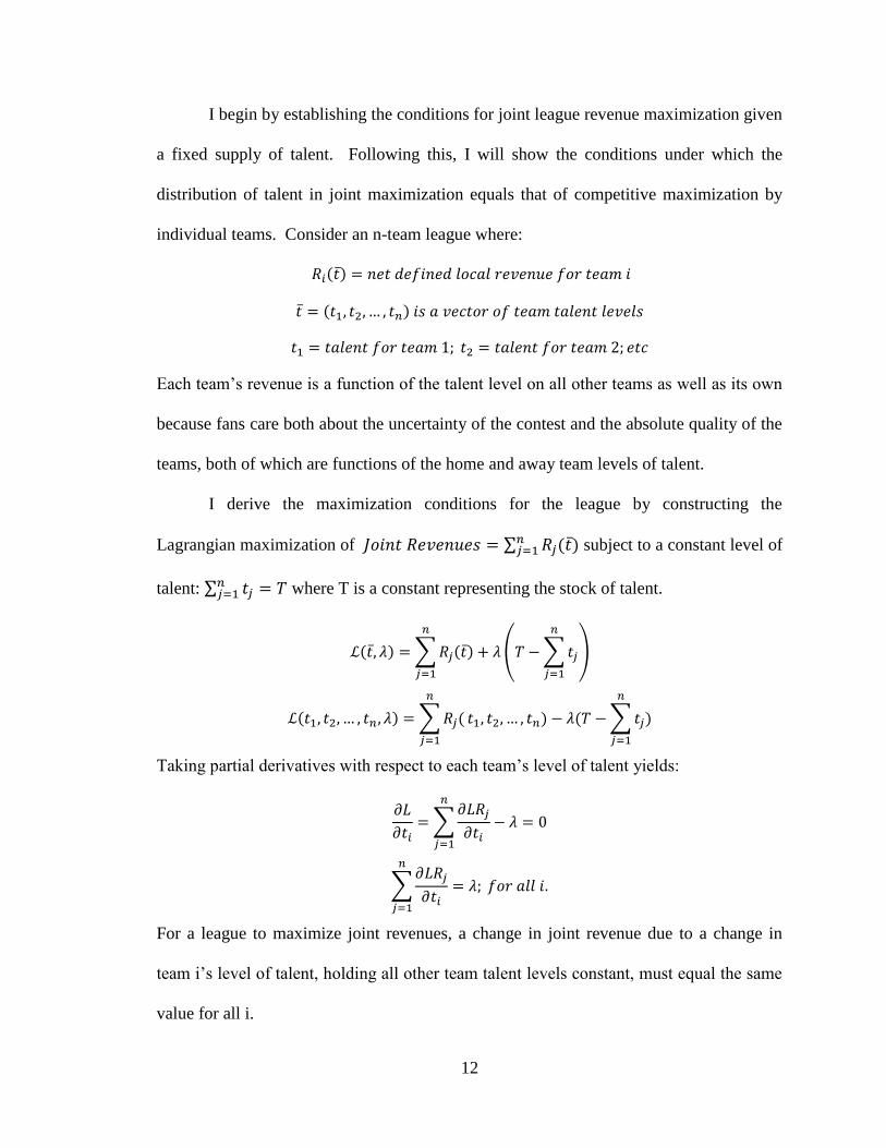
I begin by establishing the conditions for joint league revenue maximization given

a fixed supply of talent. Following this, I will show the conditions under which the

distribution of talent in joint maximization equals that of competitive maximization by

individual teams. Consider an n-team league where:

Each team‟s revenue is a function of the talent level on all other teams as well as its own

because fans care both about the uncertainty of the contest and the absolute quality of the

teams, both of which are functions of the home and away team levels of talent.

I derive the maximization conditions for the league by constructing the

Lagrangian maximization of subject to a constant level of

talent: where T is a constant representing the stock of talent.

Taking partial derivatives with respect to each team‟s level of talent yields:

For a league to maximize joint revenues, a change in joint revenue due to a change in

team i‟s level of talent, holding all other team talent levels constant, must equal the same

value for all i.

13

If the distribution of talent in joint maximization equals the distribution of talent

in competitive maximization, then teams will have no incentive to change the distribution

of talent in the presence of revenue sharing and balance will be unaffected. In the

model, I assume that teams maximize profits and that a change in talent for one team

leads to an offsetting change in the talent level of all other teams; that is,

.

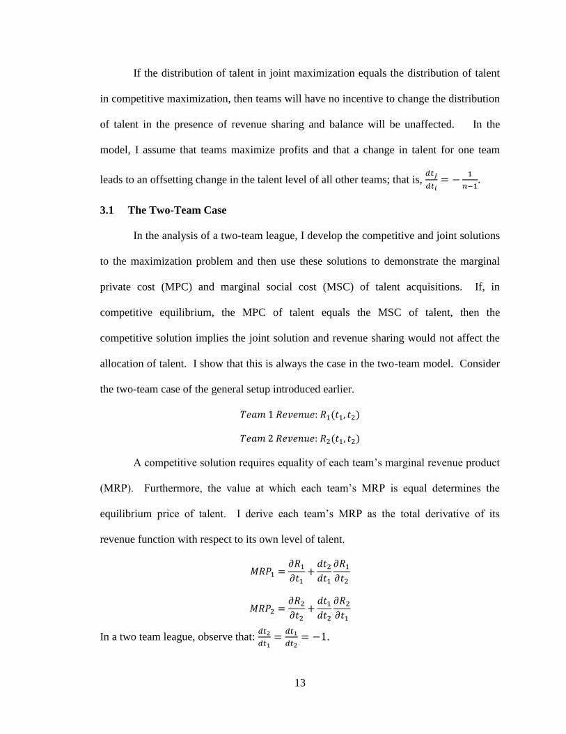
3.1 The Two-Team Case

In the analysis of a two-team league, I develop the competitive and joint solutions

to the maximization problem and then use these solutions to demonstrate the marginal

private cost (MPC) and marginal social cost (MSC) of talent acquisitions. If, in

competitive equilibrium, the MPC of talent equals the MSC of talent, then the

competitive solution implies the joint solution and revenue sharing would not affect the

allocation of talent. I show that this is always the case in the two-team model. Consider

the two-team case of the general setup introduced earlier.

A competitive solution requires equality of each team‟s marginal revenue product

(MRP). Furthermore, the value at which each team‟s MRP is equal determines the

equilibrium price of talent. I derive each team‟s MRP as the total derivative of its

revenue function with respect to its own level of talent.

In a two team league, observe that:

.

14

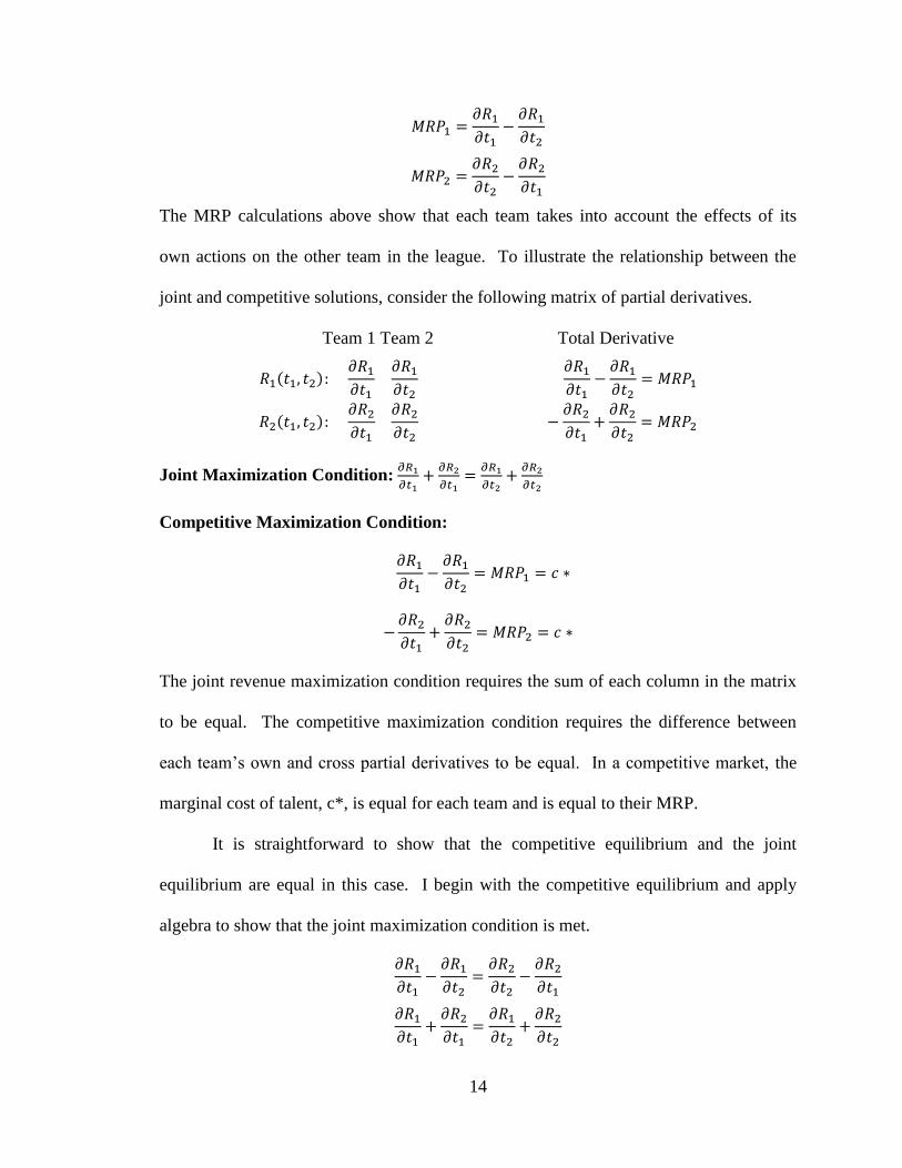
The MRP calculations above show that each team takes into account the effects of its

own actions on the other team in the league. To illustrate the relationship between the

joint and competitive solutions, consider the following matrix of partial derivatives.

Team 1 Team 2 Total Derivative

Joint Maximization Condition:

Competitive Maximization Condition:

The joint revenue maximization condition requires the sum of each column in the matrix

to be equal. The competitive maximization condition requires the difference between

each team‟s own and cross partial derivatives to be equal. In a competitive market, the

marginal cost of talent, c*, is equal for each team and is equal to their MRP.

It is straightforward to show that the competitive equilibrium and the joint

equilibrium are equal in this case. I begin with the competitive equilibrium and apply

algebra to show that the joint maximization condition is met.

15

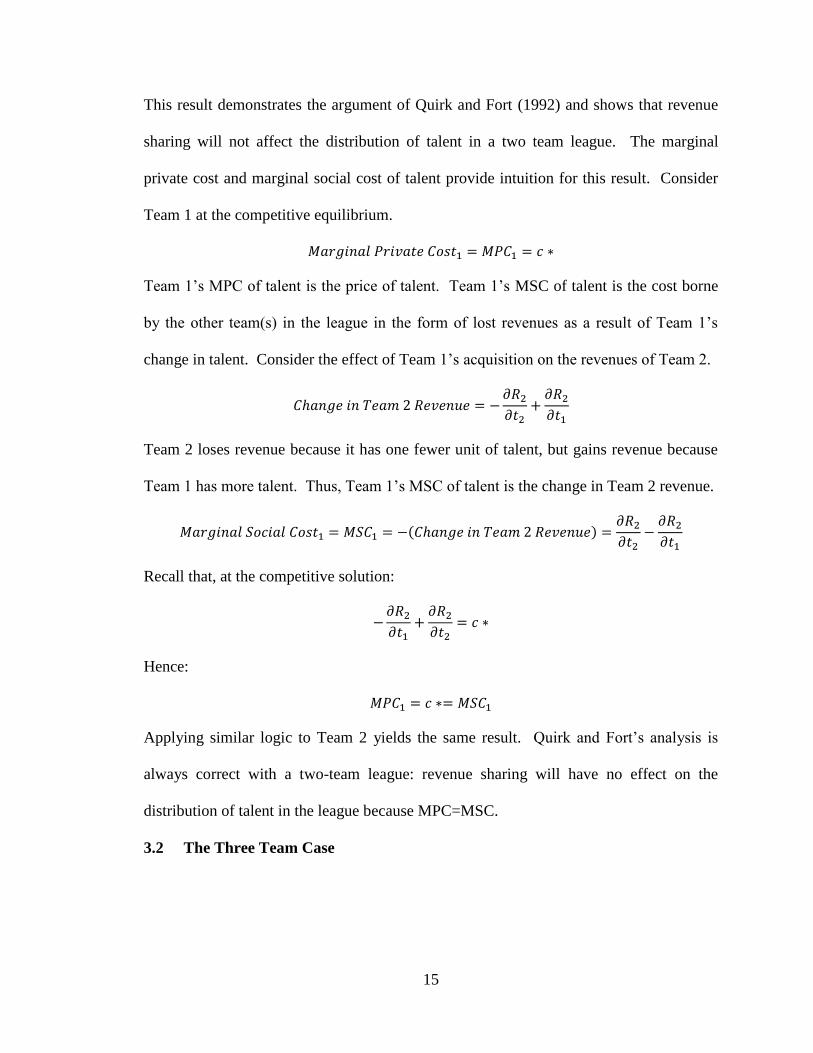
This result demonstrates the argument of Quirk and Fort (1992) and shows that revenue

sharing will not affect the distribution of talent in a two team league. The marginal

private cost and marginal social cost of talent provide intuition for this result. Consider

Team 1 at the competitive equilibrium.

Team 1‟s MPC of talent is the price of talent. Team 1‟s MSC of talent is the cost borne

by the other team(s) in the league in the form of lost revenues as a result of Team 1‟s

change in talent. Consider the effect of Team 1‟s acquisition on the revenues of Team 2.

Team 2 loses revenue because it has one fewer unit of talent, but gains revenue because

Team 1 has more talent. Thus, Team 1‟s MSC of talent is the change in Team 2 revenue.

Recall that, at the competitive solution:

Hence:

Applying similar logic to Team 2 yields the same result. Quirk and Fort‟s analysis is

always correct with a two-team league: revenue sharing will have no effect on the

distribution of talent in the league because MPC=MSC.

3.2 The Three Team Case

16

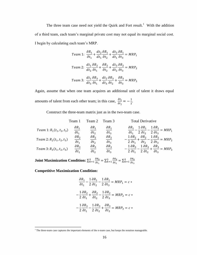
The three team case need not yield the Quirk and Fort result.1 With the addition

of a third team, each team‟s marginal private cost may not equal its marginal social cost.

I begin by calculating each team‟s MRP.

Again, assume that when one team acquires an additional unit of talent it draws equal

amounts of talent from each other team; in this case,

.

Construct the three-team matrix just as in the two-team case.

Team 1 Team 2 Team 3 Total Derivative

Joint Maximization Condition:

Competitive Maximization Condition:

1 The three-team case captures the important elements of the n-team case, but keeps the notation manageable.

17

I will use this general setup to analyze two specific cases of a three-team league, one in

which revenue sharing does not affect the distribution of talent and one in which it can.

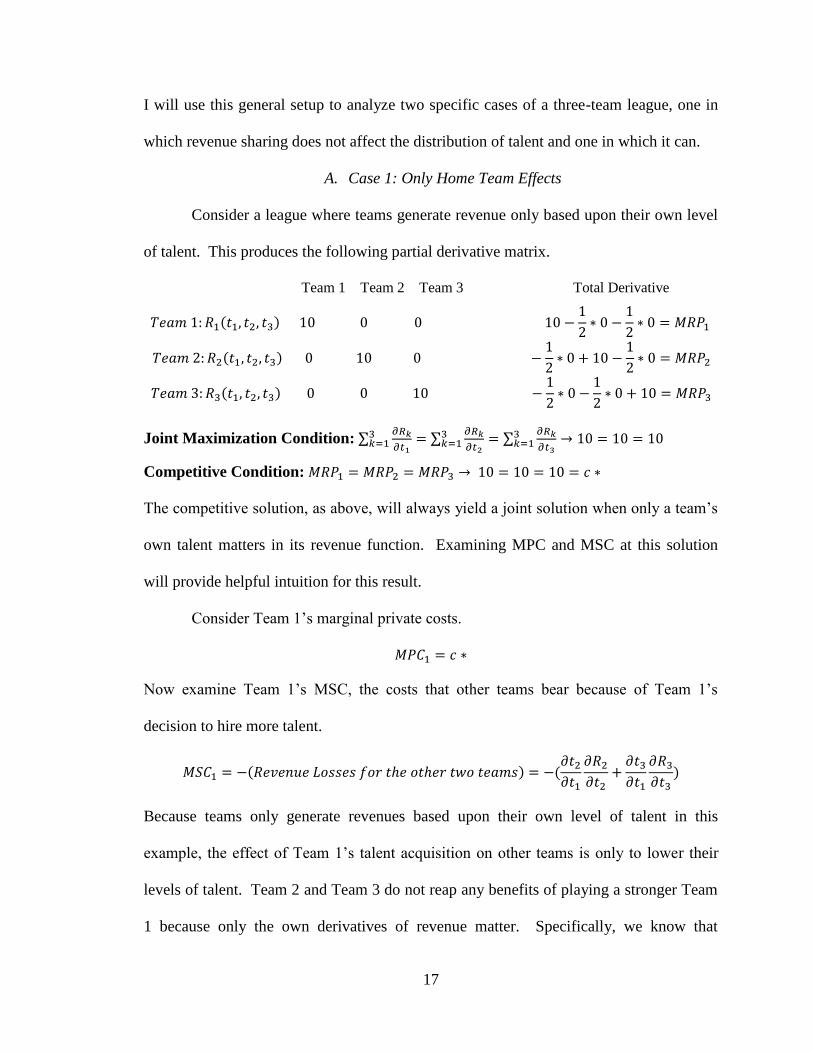
A. Case 1: Only Home Team Effects

Consider a league where teams generate revenue only based upon their own level

of talent. This produces the following partial derivative matrix.

Team 1 Team 2 Team 3 Total Derivative

Joint Maximization Condition:

Competitive Condition:

The competitive solution, as above, will always yield a joint solution when only a team‟s

own talent matters in its revenue function. Examining MPC and MSC at this solution

will provide helpful intuition for this result.

Consider Team 1‟s marginal private costs.

Now examine Team 1‟s MSC, the costs that other teams bear because of Team 1‟s

decision to hire more talent.

Because teams only generate revenues based upon their own level of talent in this

example, the effect of Team 1‟s talent acquisition on other teams is only to lower their

levels of talent. Team 2 and Team 3 do not reap any benefits of playing a stronger Team

1 because only the own derivatives of revenue matter. Specifically, we know that

18

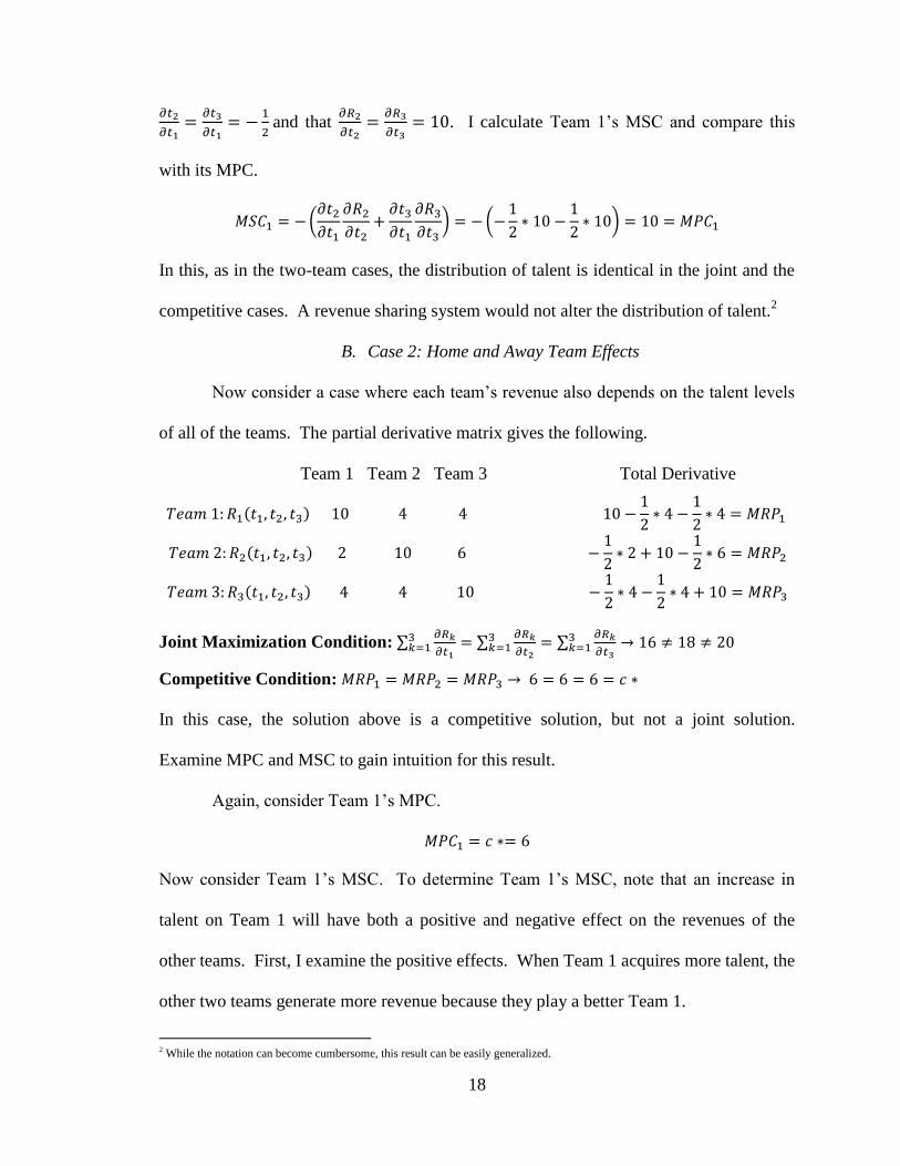
and that

. I calculate Team 1‟s MSC and compare this

with its MPC.

In this, as in the two-team cases, the distribution of talent is identical in the joint and the

competitive cases. A revenue sharing system would not alter the distribution of talent.2

B. Case 2: Home and Away Team Effects

Now consider a case where each team‟s revenue also depends on the talent levels

of all of the teams. The partial derivative matrix gives the following.

Team 1 Team 2 Team 3 Total Derivative

Joint Maximization Condition:

Competitive Condition:

In this case, the solution above is a competitive solution, but not a joint solution.

Examine MPC and MSC to gain intuition for this result.

Again, consider Team 1‟s MPC.

Now consider Team 1‟s MSC. To determine Team 1‟s MSC, note that an increase in

talent on Team 1 will have both a positive and negative effect on the revenues of the

other teams. First, I examine the positive effects. When Team 1 acquires more talent, the

other two teams generate more revenue because they play a better Team 1.

2 While the notation can become cumbersome, this result can be easily generalized.

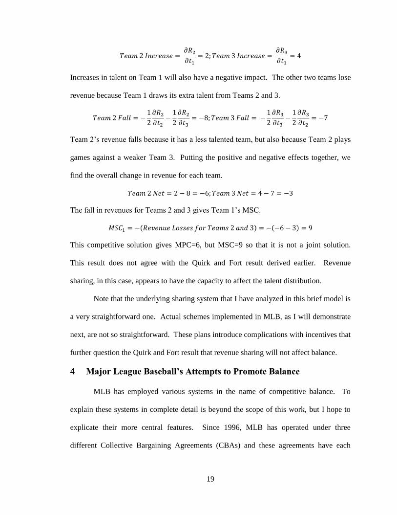
19

Increases in talent on Team 1 will also have a negative impact. The other two teams lose

revenue because Team 1 draws its extra talent from Teams 2 and 3.

Team 2‟s revenue falls because it has a less talented team, but also because Team 2 plays

games against a weaker Team 3. Putting the positive and negative effects together, we

find the overall change in revenue for each team.

The fall in revenues for Teams 2 and 3 gives Team 1‟s MSC.

This competitive solution gives MPC=6, but MSC=9 so that it is not a joint solution.

This result does not agree with the Quirk and Fort result derived earlier. Revenue

sharing, in this case, appears to have the capacity to affect the talent distribution.

Note that the underlying sharing system that I have analyzed in this brief model is

a very straightforward one. Actual schemes implemented in MLB, as I will demonstrate

next, are not so straightforward. These plans introduce complications with incentives that

further question the Quirk and Fort result that revenue sharing will not affect balance.

4 Major League Baseball’s Attempts to Promote Balance

MLB has employed various systems in the name of competitive balance. To

explain these systems in complete detail is beyond the scope of this work, but I hope to

explicate their more central features. Since 1996, MLB has operated under three

different Collective Bargaining Agreements (CBAs) and these agreements have each

20

introduced various forms of luxury taxation and revenue sharing. Not only have the

systems varied across agreements, but they have varied significantly within them, as well.

4.1 Luxury Taxes

Also called “competitive balance taxes,” luxury taxes are flat rate taxes on all

team payroll that exceeds a specified amount, called a “tax threshold.”

If team payroll > tax threshold, then:

If team payroll < tax threshold, then the team pays no tax.

Team payroll is the amount of money that

a team pays its players in a season; multi-

year contracts and signing bonuses are

spread equally throughout the contract.

Payroll also includes an equal share for

each club of the league expenditures on

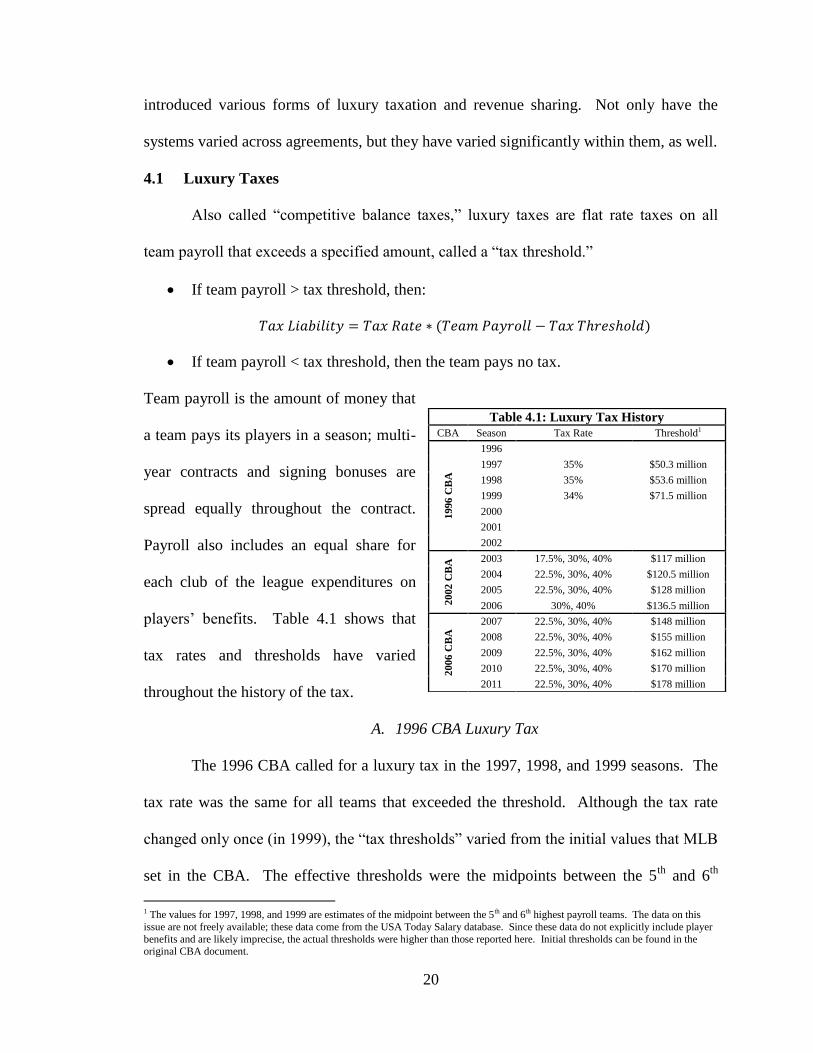
players‟ benefits. Table 4.1 shows that

tax rates and thresholds have varied

throughout the history of the tax.

A. 1996 CBA Luxury Tax

The 1996 CBA called for a luxury tax in the 1997, 1998, and 1999 seasons. The

tax rate was the same for all teams that exceeded the threshold. Although the tax rate

changed only once (in 1999), the “tax thresholds” varied from the initial values that MLB

set in the CBA. The effective thresholds were the midpoints between the 5th

and 6th

1 The values for 1997, 1998, and 1999 are estimates of the midpoint between the 5th and 6th highest payroll teams. The data on this

issue are not freely available; these data come from the USA Today Salary database. Since these data do not explicitly include player

benefits and are likely imprecise, the actual thresholds were higher than those reported here. Initial thresholds can be found in the original CBA document.

Table 4.1: Luxury Tax History

CBA Season Tax Rate Threshold1

1996

CB

A

1996

1997 35% $50.3 million

1998 35% $53.6 million

1999 34% $71.5 million

2000

2001

2002

2002

CB

A 2003 17.5%, 30%, 40% $117 million

2004 22.5%, 30%, 40% $120.5 million

2005 22.5%, 30%, 40% $128 million

2006 30%, 40% $136.5 million

2006

CB

A

2007 22.5%, 30%, 40% $148 million

2008 22.5%, 30%, 40% $155 million

2009 22.5%, 30%, 40% $162 million

2010 22.5%, 30%, 40% $170 million

2011 22.5%, 30%, 40% $178 million

21

highest payrolls in MLB.2 Revenue collected via the 1996 CBA luxury tax served many

purposes: funding shortfalls in revenue sharing payments, funding the Industry Growth

Fund, covering any disputes in the determination of luxury tax liabilities, etc.

B. 2002 CBA Competitive Balance Tax

The 2002 CBA introduced some changes to the system in addition to renaming it

a “competitive balance tax.” For one, the agreement eliminated the floating tax threshold

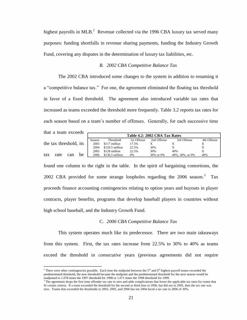
in favor of a fixed threshold. The agreement also introduced variable tax rates that

increased as teams exceeded the threshold more frequently. Table 3.2 reports tax rates for

each season based on a team‟s number of offenses. Generally, for each successive time

that a team exceeds

the tax threshold, its

tax rate can be

found one column to the right in the table. In the spirit of bargaining contortions, the

2002 CBA provided for some strange loopholes regarding the 2006 season.3 Tax

proceeds finance accounting contingencies relating to option years and buyouts in player

contracts, player benefits, programs that develop baseball players in countries without

high school baseball, and the Industry Growth Fund.

C. 2006 CBA Competitive Balance Tax

This system operates much like its predecessor. There are two main takeaways

from this system. First, the tax rates increase from 22.5% to 30% to 40% as teams

exceed the threshold in consecutive years (previous agreements did not require

2 There were other contingencies possible. Each time the midpoint between the 5th and 6th highest payroll teams exceeded the

predetermined threshold, the new threshold became the midpoint and the predetermined threshold for the next season would be readjusted to 1.078 times the 1997 threshold for 1998 or 1.071 times the 1998 threshold for 1999. 3 The agreement drops the first time offender tax rate to zero and adds complications that lower the applicable tax rates for teams that

fit certain criteria. If a team exceeded the threshold for the second or third time in 2006, but did not in 2005, then the tax rate was zero. Teams that exceeded the thresholds in 2003, 2005, and 2006 but not 2004 faced a tax rate in 2006 of 30%.

Table 4.2: 2002 CBA Tax Rates Season Threshold 1st Offense 2nd Offense 3rd Offense 4th Offense

2003 $117 million 17.5% X X X 2004 $120.5 million 22.5% 30% X X

2005 $128 million 22.5% 30% 40% X

2006 $136.5 million 0% 30% or 0% 40%, 30%, or 0% 40%

22

consecutive offenses).4 Second, the future tax rates that teams face decrease if their

payroll sinks below the payroll threshold between offenses.5 Because of the confusing

nature of the system, the CBA contains an attachment that explains every contingency.

The proceeds of this tax finance accounting issues with options and buyouts as well as

player benefits and the Industry Growth Fund.

D. Effects of the Luxury Tax

The goal of the various luxury taxes has been to make additional talent

acquisitions by large market teams more costly. We must judge the efficacy of the

system by this standard: did the tax discourage large market payroll growth. The first

luxury tax was the weakest by this standard; it did not deter payroll growth for large

market teams as much as it might have because the threshold moved upward as payrolls

increased for

the top six

teams. Teams

saved

millions

because the

effective tax

thresholds increased above the initial thresholds. In addition, the floating tax threshold

meant that no more than five teams would pay a tax.

4 There are three possible tax rates: 22.5%, 30%, and 40%. If a team exceeded the threshold in 2007 then it faced a tax rate of 22.5%

if it did not also exceed the applicable rate in 2006 in which case it faced a tax rate of 40%. In all subsequent years of the agreement, a team faces a tax rate one level higher for each consecutive year that it exceeds the applicable threshold. Thus, if a team exceeds the

threshold for the second straight year in 2010, it would face a tax rate of 30%. If that same team also exceeded the threshold in 2011,

it would face a rate of 40%. 5 For each year that a team‟s salary falls below the threshold between violations, the applicable tax rate falls one level. The previous

sentence is true except for one exception. If a club faces a 30% tax rate and then falls below the threshold and then exceeds it again in

a third year, it still faces a 30% tax rate in the third season; however, if there are two seasons between violations, then the team will face a tax rate one level lower (22.5%).

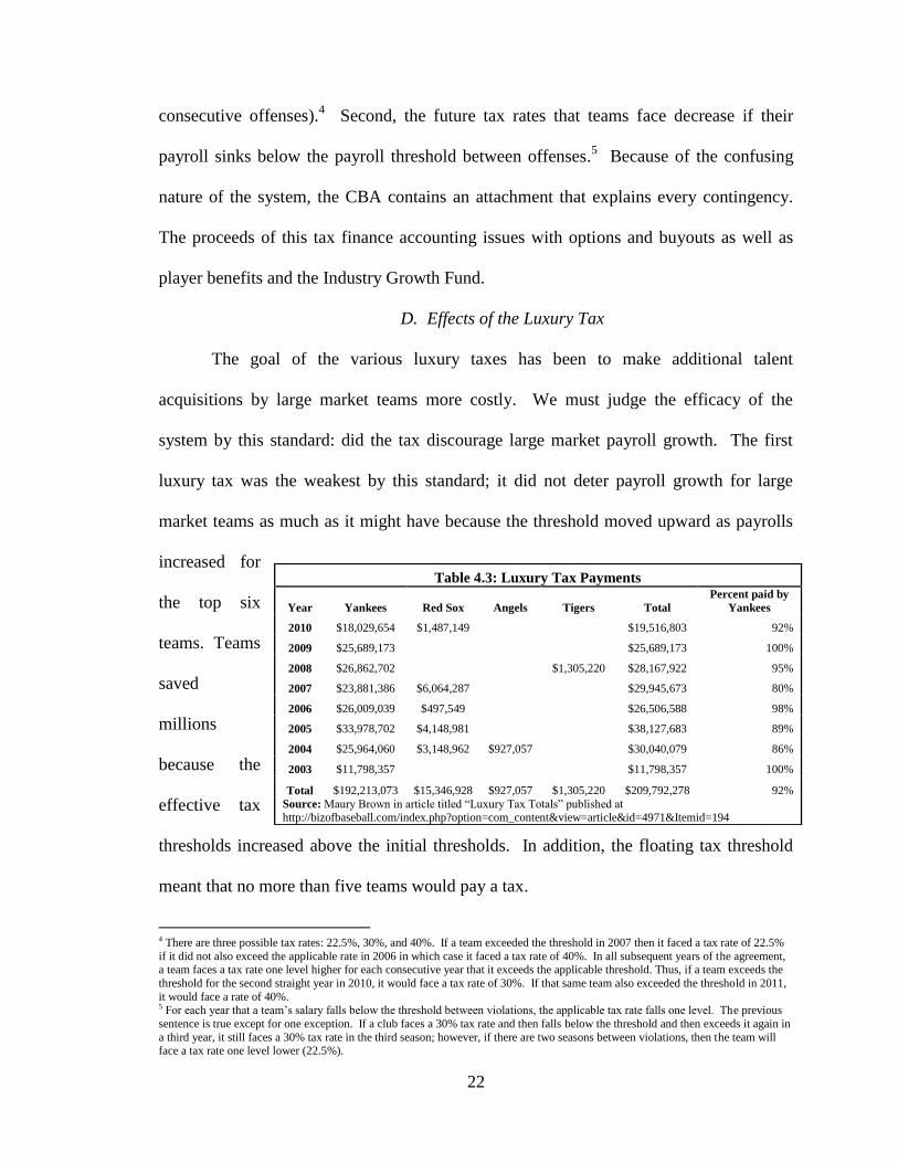
Table 4.3: Luxury Tax Payments

Year Yankees Red Sox Angels Tigers Total

Percent paid by

Yankees

2010 $18,029,654 $1,487,149

$19,516,803 92%

2009 $25,689,173

$25,689,173 100%

2008 $26,862,702

$1,305,220 $28,167,922 95%

2007 $23,881,386 $6,064,287

$29,945,673 80%

2006 $26,009,039 $497,549

$26,506,588 98%

2005 $33,978,702 $4,148,981

$38,127,683 89%

2004 $25,964,060 $3,148,962 $927,057

$30,040,079 86%

2003 $11,798,357

$11,798,357 100%

Total $192,213,073 $15,346,928 $927,057 $1,305,220 $209,792,278 92%

Source: Maury Brown in article titled “Luxury Tax Totals” published at http://bizofbaseball.com/index.php?option=com_content&view=article&id=4971&Itemid=194

23

The next two versions are very similar to each other. Both the 2002 and 2006

versions instituted both an increasing tax rate that punished repeat offenders and a fixed

tax threshold that served as a harder cap on payrolls. Although the fixed thresholds in

these systems likely increased the efficacy of the “competitive balance tax,” they were set

so high that many regard these systems as “Yankee taxes.” Table 4.3 shows estimates of

luxury tax payments provided by bizofbaseball.com. As the data show, the Yankees paid

at least 80% of the league total in each season from 2003-2010. In total, only three other

teams paid anything under the systems. The Yankees luxury tax bill has grown so large

at times that it exceeded the entire team payroll of the Devil Rays in 2005. The Yankees

continue to lead the league in payroll annually, but such large luxury tax payments likely

caused the front office to think twice about additional talent acquisitions.

The luxury tax diminishes large market valuations of players; this should

compress salaries at the top of the distribution, but it will not provide incentives to small

market teams to spend more on talent. Revenue Sharing, on the other hand, was designed

with the hope that it would encourage payroll expansion at the bottom of the revenue

distribution as well as curtail spending at the top.

4.2 Revenue Sharing

MLB also uses revenue sharing to redistribute hundreds of millions of dollars

each season. To understand these systems, we first examine sources of team revenue.

A. Definitions

MLB‟s revenue sharing system redistributes both “central fund revenue” and a

portion of individual team revenue called “net defined local revenue” (NDLR).

24

- Central Fund Revenue: items like national broadcasting contracts and central

licensing through MLB Properties.

- NDLR: all “defined gross revenue” minus central fund revenue and stadium

expenses.

- Defined gross revenues: revenue not limited to ticket sales, but including all

revenues generated by the team “except those wholly unrelated to the business of

Major League Baseball.”

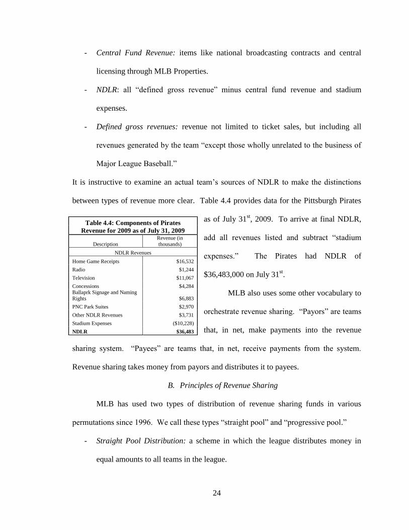
It is instructive to examine an actual team‟s sources of NDLR to make the distinctions

between types of revenue more clear. Table 4.4 provides data for the Pittsburgh Pirates

as of July 31st, 2009. To arrive at final NDLR,

add all revenues listed and subtract “stadium

expenses.” The Pirates had NDLR of

$36,483,000 on July 31st.

MLB also uses some other vocabulary to

orchestrate revenue sharing. “Payors” are teams

that, in net, make payments into the revenue

sharing system. “Payees” are teams that, in net, receive payments from the system.

Revenue sharing takes money from payors and distributes it to payees.

B. Principles of Revenue Sharing

MLB has used two types of distribution of revenue sharing funds in various

permutations since 1996. We call these types “straight pool” and “progressive pool.”

- Straight Pool Distribution: a scheme in which the league distributes money in

equal amounts to all teams in the league.

Table 4.4: Components of Pirates

Revenue for 2009 as of July 31, 2009

Description

Revenue (in

thousands)

NDLR Revenues

Home Game Receipts $16,532

Radio $1,244

Television $11,067

Concessions $4,284

Ballaprk Signage and Naming

Rights $6,883

PNC Park Suites $2,970

Other NDLR Revenues $3,731

Stadium Expenses ($10,228)

NDLR $36,483

25

- Progressive Pool Distribution: a scheme in which the league distributes money to

teams based upon some measure of their financial strength.6

The league generates money for these pools with any combination of a tax on NDLR and

central fund revenue.

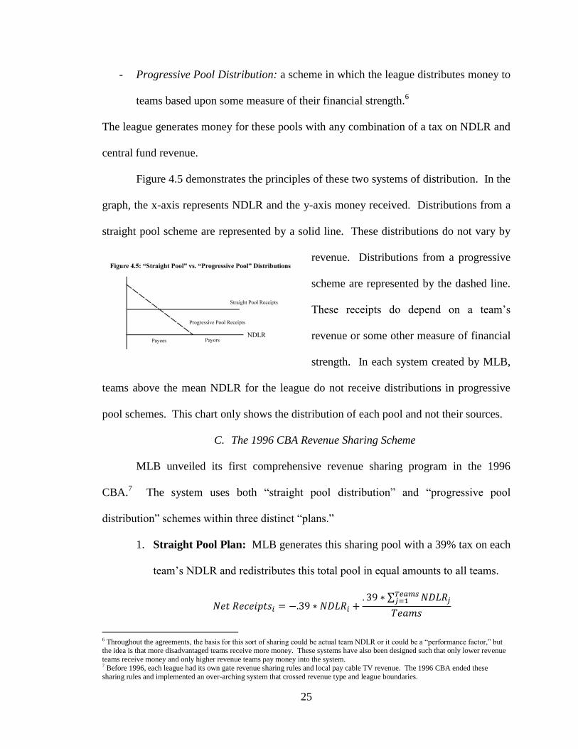
Figure 4.5 demonstrates the principles of these two systems of distribution. In the

graph, the x-axis represents NDLR and the y-axis money received. Distributions from a

straight pool scheme are represented by a solid line. These distributions do not vary by

revenue. Distributions from a progressive

scheme are represented by the dashed line.

These receipts do depend on a team‟s

revenue or some other measure of financial

strength. In each system created by MLB,

teams above the mean NDLR for the league do not receive distributions in progressive

pool schemes. This chart only shows the distribution of each pool and not their sources.

C. The 1996 CBA Revenue Sharing Scheme

MLB unveiled its first comprehensive revenue sharing program in the 1996

CBA.7 The system uses both “straight pool distribution” and “progressive pool

distribution” schemes within three distinct “plans.”

1. Straight Pool Plan: MLB generates this sharing pool with a 39% tax on each

team‟s NDLR and redistributes this total pool in equal amounts to all teams.

6 Throughout the agreements, the basis for this sort of sharing could be actual team NDLR or it could be a “performance factor,” but the idea is that more disadvantaged teams receive more money. These systems have also been designed such that only lower revenue

teams receive money and only higher revenue teams pay money into the system. 7 Before 1996, each league had its own gate revenue sharing rules and local pay cable TV revenue. The 1996 CBA ended these sharing rules and implemented an over-arching system that crossed revenue type and league boundaries.

26

2. Split Pool Plan: MLB generates this sharing pool with a 20% tax on each

team‟s NDLR. MLB distributes 75% of this pool on a “straight pool” basis.

The league distributes the remaining 25% only to teams below the mean

NDLR in proportion to how far a team‟s NDLR falls below the league mean.

Teams above the league mean NDLR only receive “straight pool payments:

Teams below the league mean NDLR receive both straight pool and

progressive pool payments:

3. Hybrid Pool Plan8: This plan calculates the outcome for each team under

both the “Straight Pool” plan and the “Split Pool” plan and then assigns net

receipts to that team based upon the more favorable outcome.

The manner in which MLB redistributes money to payee teams in the “Split Pool

Plan” follows a formula that will form the basis of MLB‟s subsequent “progressive”

distributions. Focus on the final term in the net receipts equation for payees above. This

term is equal to the size of the pool to be redistributed (

multiplied by a “reallocation proportion” (

). As a

payee team generates more revenue, its reallocation proportion falls and it receives less

8 This system created a “shortfall” because there were not enough payments to cover payouts. The league covered the shortfall with “superstation settlement” payments.

27

money. The history of the changes to the revenue sharing system in MLB can be

understood largely as a debate over how to calculate the reallocation proportion.

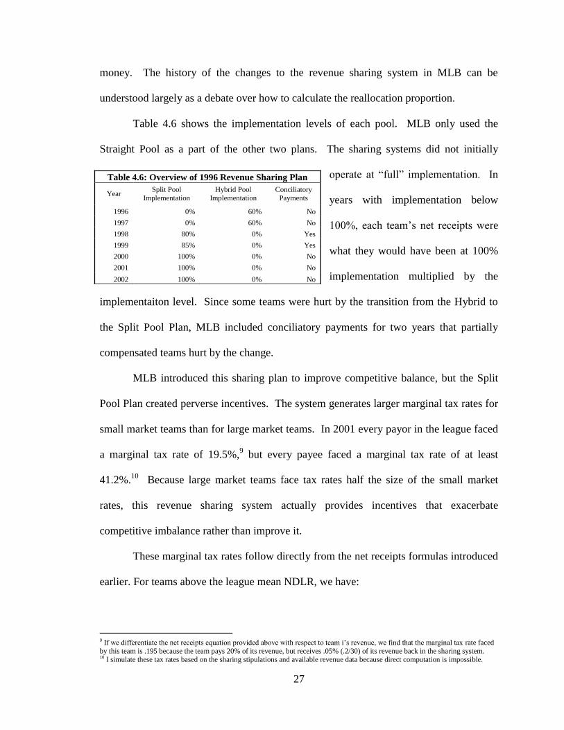
Table 4.6 shows the implementation levels of each pool. MLB only used the

Straight Pool as a part of the other two plans. The sharing systems did not initially

operate at “full” implementation. In

years with implementation below

100%, each team‟s net receipts were

what they would have been at 100%

implementation multiplied by the

implementaiton level. Since some teams were hurt by the transition from the Hybrid to

the Split Pool Plan, MLB included conciliatory payments for two years that partially

compensated teams hurt by the change.

MLB introduced this sharing plan to improve competitive balance, but the Split

Pool Plan created perverse incentives. The system generates larger marginal tax rates for

small market teams than for large market teams. In 2001 every payor in the league faced

a marginal tax rate of 19.5%,9 but every payee faced a marginal tax rate of at least

41.2%.10

Because large market teams face tax rates half the size of the small market

rates, this revenue sharing system actually provides incentives that exacerbate

competitive imbalance rather than improve it.

These marginal tax rates follow directly from the net receipts formulas introduced

earlier. For teams above the league mean NDLR, we have:

9 If we differentiate the net receipts equation provided above with respect to team i‟s revenue, we find that the marginal tax rate faced

by this team is .195 because the team pays 20% of its revenue, but receives .05% (.2/30) of its revenue back in the sharing system. 10 I simulate these tax rates based on the sharing stipulations and available revenue data because direct computation is impossible.

Table 4.6: Overview of 1996 Revenue Sharing Plan

Year Split Pool

Implementation

Hybrid Pool

Implementation

Conciliatory

Payments

1996 0% 60% No

1997 0% 60% No

1998 80% 0% Yes

1999 85% 0% Yes

2000 100% 0% No

2001 100% 0% No

2002 100% 0% No

28

For teams below the league mean NDLR, we have:

The two equations are identical except for the “reallocation proportion” in the second

equation; this term creates the perverse incentives. When a payee hires more talent to

increase NDLR, its net receipts rise by less than that of a payor making an identical hire.

As a consequence of the “reallocation proportion” in the above equation, payees have less

incentive to hire talent than payors. Due to these incentives, some small market teams

find that lowering expenditures on payroll is a profit maximizing strategy even if it

results in decreased revenue. Zimbalist writes, “if the reduction in payroll plus the

additional revenue sharing transfer exceed the drop in team revenue, then lowballing

payroll would be a maximizing strategy.” (Zimbalist 2003, 91)

The incentive effects of the marginal tax rates would not worsen balance if MLB

had a credible way to force payees to use their revenue sharing receipts to hire more

talent. The 1996 CBA gave the commissioner responsibility to ensure that payees spent

revenue sharing receipts on improving their team. Commissioner Bud Selig has publicly

affirmed this responsibility. This is troubling, however, because Selig‟s team, the

Milwaukee Brewers, was one of the prime offenders. Additionally, teams like the Devil

Rays often spent revenue sharing money on the franchise by covering other costs, like

debt payments, but not increasing expenditures on players (Zimbalist 2003).

29

D. The 2002 CBA Revenue Sharing System

As a consequence of the concern expressed by the Commissioner‟s Blue Ribbon

Panel on the Economics of Baseball, the owners and players created a new revenue

sharing system in 2002. While this plan

transferred even more money, it did not

remedy the incentive problems. The new

system had two main components,11

the

“Base Plan” and a supplemental pool.12

The “Base Plan” was a simple “straight

pool” scheme with a 34% tax on each

team‟s NDLR. The supplemental pool was

more complicated created the incentive

problems.

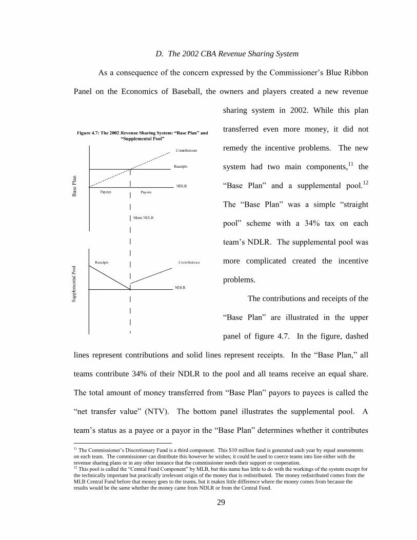
The contributions and receipts of the

“Base Plan” are illustrated in the upper

panel of figure 4.7. In the figure, dashed

lines represent contributions and solid lines represent receipts. In the “Base Plan,” all

teams contribute 34% of their NDLR to the pool and all teams receive an equal share.

The total amount of money transferred from “Base Plan” payors to payees is called the

“net transfer value” (NTV). The bottom panel illustrates the supplemental pool. A

team‟s status as a payee or a payor in the “Base Plan” determines whether it contributes

11 The Commissioner‟s Discretionary Fund is a third component. This $10 million fund is generated each year by equal assessments

on each team. The commissioner can distribute this however he wishes; it could be used to coerce teams into line either with the

revenue sharing plans or in any other instance that the commissioner needs their support or cooperation. 12 This pool is called the “Central Fund Component” by MLB, but this name has little to do with the workings of the system except for

the technically important but practically irrelevant origin of the money that is redistributed. The money redistributed comes from the

MLB Central Fund before that money goes to the teams, but it makes little difference where the money comes from because the results would be the same whether the money came from NDLR or from the Central Fund.

30

money to or receives money from the supplemental pool. Payors in the “Base Plan”

contribute money to the supplemental pool.13

The pool generated above is then distributed to “Base Plan” payees.

Only payees receive money in the supplemental pool and only payors contribute

money.14

These formulas follow the template outlined previously. Each redistributive

formula includes the size of the pool to be redistributed ( ) and a

“redistribution proportion” that differs depending on whether a team contributes to the

pool or receives from it. As a payee generates more revenue, its “reallocation

proportion” falls and it receives less money. Conversely, as a payor generates more

revenue, its “reallocation proportion” rises and it must contribute more.

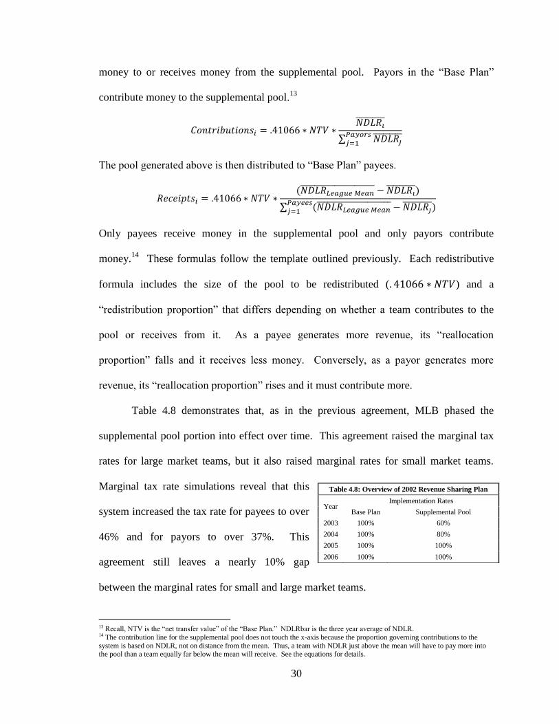
Table 4.8 demonstrates that, as in the previous agreement, MLB phased the

supplemental pool portion into effect over time. This agreement raised the marginal tax

rates for large market teams, but it also raised marginal rates for small market teams.

Marginal tax rate simulations reveal that this

system increased the tax rate for payees to over

46% and for payors to over 37%. This

agreement still leaves a nearly 10% gap

between the marginal rates for small and large market teams.

13 Recall, NTV is the “net transfer value” of the “Base Plan.” NDLRbar is the three year average of NDLR. 14 The contribution line for the supplemental pool does not touch the x-axis because the proportion governing contributions to the

system is based on NDLR, not on distance from the mean. Thus, a team with NDLR just above the mean will have to pay more into the pool than a team equally far below the mean will receive. See the equations for details.

Table 4.8: Overview of 2002 Revenue Sharing Plan

Year Implementation Rates

Base Plan Supplemental Pool

2003 100% 60%

2004 100% 80%

2005 100% 100%

2006 100% 100%

31

E. The 2006 CBA Revenue Sharing System

The 2006 CBA keeps the “Base Plan” largely the same as in the 2002 system, but

makes changes to the supplemental pool that realign incentives to begin to improve

competitive balance.15

The redesign of the supplemental pool lowers marginal tax rates

for both large and small market teams from the levels of the 2002 agreement and actually

reduces the tax rates for small market teams to levels below those for large market teams.

The only change to the “Base Plan” is that its tax rate is lowered to 31% from

34%. Because the perverse balance incentives of previous agreements originated in the

progressive portions of the systems, this CBA changes the way the supplemental pool

allocates funds. Consider the template we introduced earlier.

16

In past agreements, the reallocation proportion was some measure of a team‟s financial

success in a particular season relative to the rest of the league. In the new agreement, this

proportion is called a “Performance Factor” and it is fixed ahead of time. For example,

the Yankees “Performance Factor” dictates that they contribute about 22% of the pool

while the Rays‟ factor calls for them to receive about 10%. “Performance Factors” are

specified in the CBA, they are determined using revenue data from 2004, 2005, and

extrapolations for 2006 and 2007, and they are only subject to change under unusual

circumstances.17

Because “Performance Factors” are set in advance, a team could be a

payee in the “Base Plan” and a payor in the supplemental pool, or vice versa.

15 Once again, this is what MLB calls “the Central Fund Component.” This agreement also keeps the commissioner‟s discretionary fund in place just as in the 2002 agreement. 16 In the 2002 agreement, for contributors this proportion was the three year mean NDLR over the sum of all such NDLRs for all

payors. For recipients, this proportion was the difference between the three year league mean NDLR and the team‟s three year mean NDLR over the sum of this calculation for all payees. 17 Performance factors can change in the midst of a CBA for two reasons. The first situation is one in which the team builds a new

stadium; in this case, new performance factors take effect for the team (and the league as a whole) in the second year after the completion of the stadium. The new factors are based upon 90% of the team‟s revenue in its stadium‟s inaugural year. The second

32

This CBA also changes the way that the size of the supplemental pool is

determined. In short, the amount of money transferred from payors to payees, the “net

transfer value,” in the entire sharing system, including both the “Base Plan” and the

supplemental pool, must equal the NTV of a hypothetical straight pool plan with a tax

rate of 48%.18

Since the NTV of the “Base Plan” is already determined, the supplemental

pool size varies to achieve the desired NTV for the whole system.19

This sharing plan lowers the marginal tax rate faced by payees. Tax rates for the

lowest revenue teams fall to around 30% while marginal tax rates on the highest revenue

teams hover around 32.5%. The institution of a slightly progressive marginal tax rate

should finally augment small market incentives to spend relative to large market

incentives.

While the 2006 system alleviates the marginal tax rate problem, it does not draw a

distinction between “good” and “bad” imbalance. Recall the distinction that Stefan

Kesenne draws between “good” and “bad” imbalance: “good” imbalance occurs when a

small market team wins regularly through good management while “bad” imbalance

occurs when a large market team wins regularly through the advantages that it has in

market strength. Kesenne argues that when leagues introduce revenue sharing, they

generally seek to remedy “bad” imbalance, but that this may lead to “curing” a “good”

imbalance and turning it into a “bad” one. The 2006 CBA risks turning a “good”

imbalance into a “bad” one. For example, the Detroit Tigers play in one of baseball‟s

stronger markets; the Tigers had the second highest payroll in Major League Baseball in

situation is one in which a team‟s compound annual growth rate of revenue exceeds or lags the MLB average by at least 10 points in

each season over the course of three years. 18 Taken together, the NTV of the “Base Plan” and supplemental pool must equal what the NTV would be under a hypothetical sharing scheme that was a straight pool with a tax rate of 48%. This does not mean that each team receives what they would under

such a scheme, but that the total amount transferred must equal the amount under this hypothetical scheme. 19 In cases where a team is a payor in the “Base Plan” and a payee in the supplemental pool (or vice versa), the supplemental pool is changed with compensating for this difference to achieve the proper total NTV.

33

2008 and played in the World Series in 2006. However, the Tigers performed poorly in

the period used to calculate performance factors and thus they receive payments in the

supplemental portion of revenue sharing. The Tigers performed poorly in the period used

to calculate performance because they displayed poor management. Thus, the 2006

revenue sharing plan appears to have mistaken a “good” imbalance for a “bad” one.

5 Empirical Data Analysis

Only a revenue sharing system based upon market strength can avoid mistaking a

“good” imbalance for a “bad” one. Thus, the goals of this chapter include: develop an

econometric model of revenue generation and use this to demonstrate the ways in which

the 2006 CBA “cures” good imbalances. After developing an index of market strength I

use this index to show that MLB‟s revenue sharing schemes have had adverse effects on

competitive balance.

5.1 Data

Because MLB teams are private businesses that jealously guard their finances,

team revenue is rarely disclosed. Consequently, I have pieced together data1, some of

which are actual revenues and some of which are estimates. Data from 1990 and 1992-

1994 are based on reports from Financial World Magazine that have been adjusted to

account for central fund revenue; 1991 data is from The Sporting News and is adjusted in

the same fashion. 1995-2001 data is actual data that was reported in the Blue Ribbon

Panel Report to the Commissioner. 2002-2009 data come from Forbes Magazine and

have been adjusted for central fund revenues and for revenue sharing transfers.2

1 The revenue data are “defined gross revenue” minus central revenue and minus revenue sharing. 2 Data from before 1995 were relatively straightforward to adjust because no revenue sharing agreement was in effect. Thus, I

subtracted central revenues from each team. Data after 2001, however, was more difficult. The data reported by Forbes are estimates

of revenue post central fund revenues and post revenue sharing. These pieces of data were estimated with the help of Professor Frank Westhoff and Professor Andrew Zimbalist.

34

5.2 Choice of Model

It will be nearly impossible to account for all of the unobserved differences

among teams and markets. Fortunately, many of these unobservable characteristics

persist throughout time. Thus, a fixed effects model with controls for both team and time

is well suited to the task of estimating revenue. A team effects model will perform better

than a city effects model because unobserved effects derive at the team level.

Cities with multiple teams demonstrate why I use team, not city, fixed effects.

The White Sox and Cubs share a similar market in Chicago and the White Sox even have

a newer stadium with more revenue generating possibilities. The White Sox have

achieved more success in both the regular season and the playoffs than the Cubs.3 Yet,

despite the advantages on the South Side (White Sox), the North Side (Cubs) has

generated more revenue in every season since 1997 and outdrawn at the gate in every

season since 1992.

5.3 Specification of the Model

To analyze MLB team revenue, I consolidate potential regressors into six

categories. These categories include current season performance, expectations about the

upcoming season, historical performance, stadium quality, market strength, and other

unobserved team characteristics.4 The general equation is as follows.

3 The Cubs have averaged about 78 wins per season since 1988 while the White Sox have averaged about 83. Furthermore, the White Sox won the World Series in 2005 while the Cubs have not won the World Series in over 100 years. Since 1988, the Cubs have made

the playoffs five times while the White Sox have made the playoffs four times. 4 F-tests reveal that these categories are significant except for historical performance. Surprisingly, F-tests on the GLS results show that market characteristics are not significant in the GLS specifications.

35

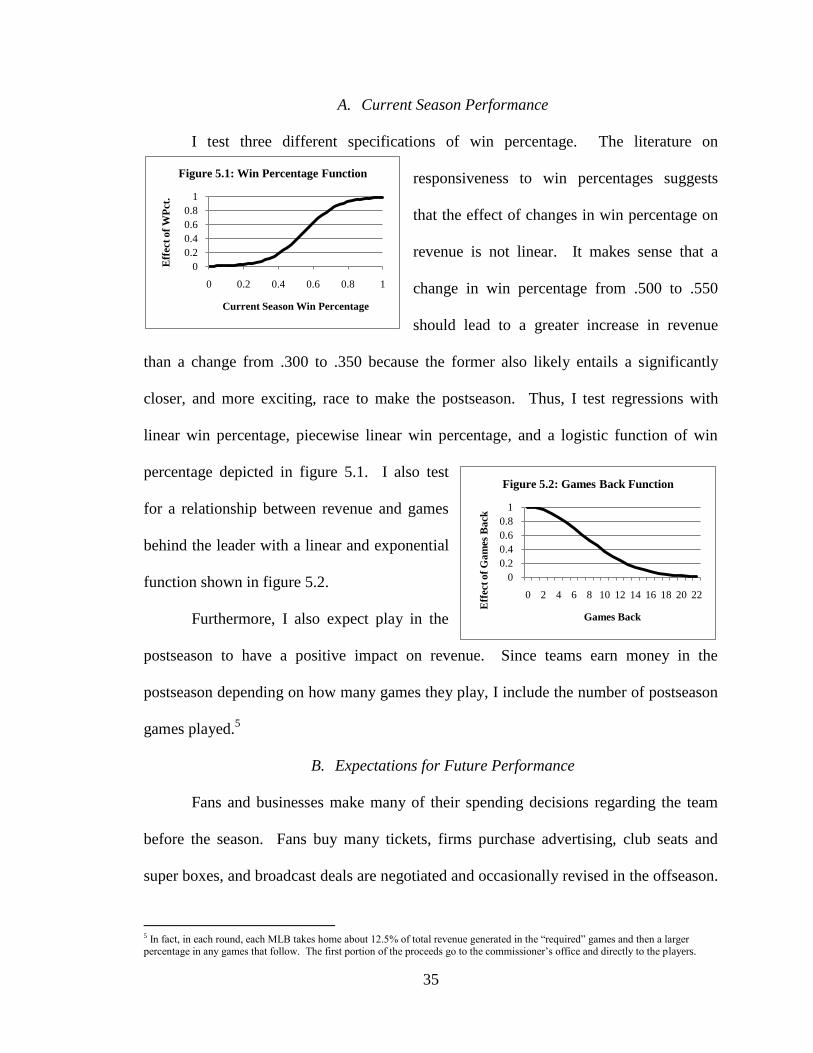
A. Current Season Performance

I test three different specifications of win percentage. The literature on

responsiveness to win percentages suggests

that the effect of changes in win percentage on

revenue is not linear. It makes sense that a

change in win percentage from .500 to .550

should lead to a greater increase in revenue

than a change from .300 to .350 because the former also likely entails a significantly

closer, and more exciting, race to make the postseason. Thus, I test regressions with

linear win percentage, piecewise linear win percentage, and a logistic function of win

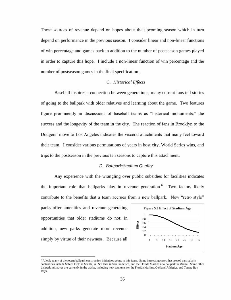
percentage depicted in figure 5.1. I also test

for a relationship between revenue and games

behind the leader with a linear and exponential

function shown in figure 5.2.

Furthermore, I also expect play in the

postseason to have a positive impact on revenue. Since teams earn money in the

postseason depending on how many games they play, I include the number of postseason

games played.5

B. Expectations for Future Performance

Fans and businesses make many of their spending decisions regarding the team

before the season. Fans buy many tickets, firms purchase advertising, club seats and

super boxes, and broadcast deals are negotiated and occasionally revised in the offseason.

5 In fact, in each round, each MLB takes home about 12.5% of total revenue generated in the “required” games and then a larger percentage in any games that follow. The first portion of the proceeds go to the commissioner‟s office and directly to the players.

0

0.2

0.4

0.6

0.8

1

0 0.2 0.4 0.6 0.8 1

Eff

ect

of

WP

ct.

Current Season Win Percentage

Figure 5.1: Win Percentage Function

0

0.2

0.4

0.6

0.8

1

0 2 4 6 8 10 12 14 16 18 20 22

Eff

ect

of

Ga

mes

Ba

ck

Games Back

Figure 5.2: Games Back Function

36

These sources of revenue depend on hopes about the upcoming season which in turn

depend on performance in the previous season. I consider linear and non-linear functions

of win percentage and games back in addition to the number of postseason games played

in order to capture this hope. I include a non-linear function of win percentage and the

number of postseason games in the final specification.

C. Historical Effects

Baseball inspires a connection between generations; many current fans tell stories

of going to the ballpark with older relatives and learning about the game. Two features

figure prominently in discussions of baseball teams as “historical monuments:” the

success and the longevity of the team in the city. The reaction of fans in Brooklyn to the

Dodgers‟ move to Los Angeles indicates the visceral attachments that many feel toward

their team. I consider various permutations of years in host city, World Series wins, and

trips to the postseason in the previous ten seasons to capture this attachment.

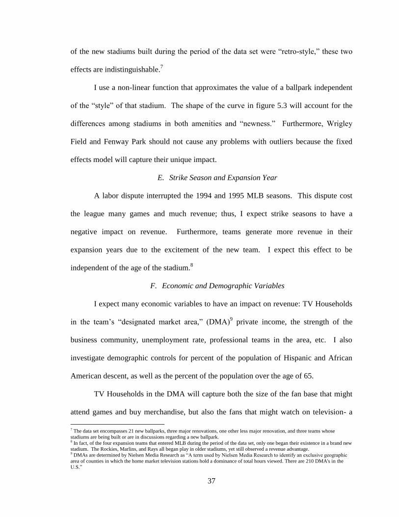
D. Ballpark/Stadium Quality

Any experience with the wrangling over public subsidies for facilities indicates

the important role that ballparks play in revenue generation.6 Two factors likely

contribute to the benefits that a team accrues from a new ballpark. New “retro style”

parks offer amenities and revenue generating

opportunities that older stadiums do not; in

addition, new parks generate more revenue

simply by virtue of their newness. Because all

6 A look at any of the recent ballpark construction initiatives points to this issue. Some interesting cases that proved particularly

contentious include Safeco Field in Seattle, AT&T Park in San Francisco, and the Florida Marlins new ballpark in Miami. Some other

ballpark initiatives are currently in the works, including new stadiums for the Florida Marlins, Oakland Athletics, and Tampa Bay Rays.

0

0.2

0.4

0.6

0.8

1

1 6 11 16 21 26 31 36

Eff

ect

Stadium Age

Figure 5.3 Effect of Stadium Age

37

of the new stadiums built during the period of the data set were “retro-style,” these two

effects are indistinguishable.7

I use a non-linear function that approximates the value of a ballpark independent

of the “style” of that stadium. The shape of the curve in figure 5.3 will account for the

differences among stadiums in both amenities and “newness.” Furthermore, Wrigley

Field and Fenway Park should not cause any problems with outliers because the fixed

effects model will capture their unique impact.

E. Strike Season and Expansion Year

A labor dispute interrupted the 1994 and 1995 MLB seasons. This dispute cost

the league many games and much revenue; thus, I expect strike seasons to have a

negative impact on revenue. Furthermore, teams generate more revenue in their

expansion years due to the excitement of the new team. I expect this effect to be

independent of the age of the stadium.8

F. Economic and Demographic Variables

I expect many economic variables to have an impact on revenue: TV Households

in the team‟s “designated market area,” (DMA)9 private income, the strength of the

business community, unemployment rate, professional teams in the area, etc. I also

investigate demographic controls for percent of the population of Hispanic and African

American descent, as well as the percent of the population over the age of 65.

TV Households in the DMA will capture both the size of the fan base that might

attend games and buy merchandise, but also the fans that might watch on television- a

7 The data set encompasses 21 new ballparks, three major renovations, one other less major renovation, and three teams whose

stadiums are being built or are in discussions regarding a new ballpark. 8 In fact, of the four expansion teams that entered MLB during the period of the data set, only one began their existence in a brand new stadium. The Rockies, Marlins, and Rays all began play in older stadiums, yet still observed a revenue advantage. 9 DMAs are determined by Nielsen Media Research as “A term used by Nielsen Media Research to identify an exclusive geographic

area of counties in which the home market television stations hold a dominance of total hours viewed. There are 210 DMA's in the U.S.”

38

very important part of revenue generation for teams given the rise in the value of TV

rights. The aggregate income data are a good approximation of the aggregate income of

fans likely to support the team.10

I include the number of businesses in the area because

businesses purchase advertisements, season tickets, club seats, and luxury boxes at the

park. Unemployment rate serves to capture general economic conditions. The effect of

number of professional teams in the area is important and should be negative because

businesses and residents have more options for their advertising and entertainment

spending when more teams are present.

Results in the literature have shown that percent African American has a negative

impact on attendance (Noll 1974, 121). Thus, I include this variable as well as a variable

for percent Hispanic because of the growing Hispanic population in many cities and the

popularity of baseball in many Latin American countries. The variable for percent over

65 may capture problems that teams like the Rays, Marlins, and Diamondbacks face due

to an older fan base.11

The effect of this variable may be confounded because MLB‟s fan

base in general is older than the other sports.

5.4 Results

Despite its merits, the typical fixed effects model discussed earlier has some

drawbacks. A test derived by Wooldridge (2002) to check for autocorrelation shows that

OLS is not the best linear unbiased estimator of the model. Consequently, I report both

the standard OLS fixed effects results with heteroskedasticity robust standard errors in

regressions (1-3) and the results for a GLS fixed effects model that uses Cochrane-Orcutt

to account for autocorrelation in regressions (4-6) of table 5.1. The overall effect of each

10 These data are the average of total income within a 5 mile radius around the stadium, a 15 mile radius, and a 30 mile radius. 11 Large numbers of retirees in markets means two things for baseball game attendance. First, these fans may be less able to make it to

the ballpark and when they do, they are less likely to spend money. Second, many of these fans have loyalties that lie elsewhere, since retirees often still root for their home town teams.

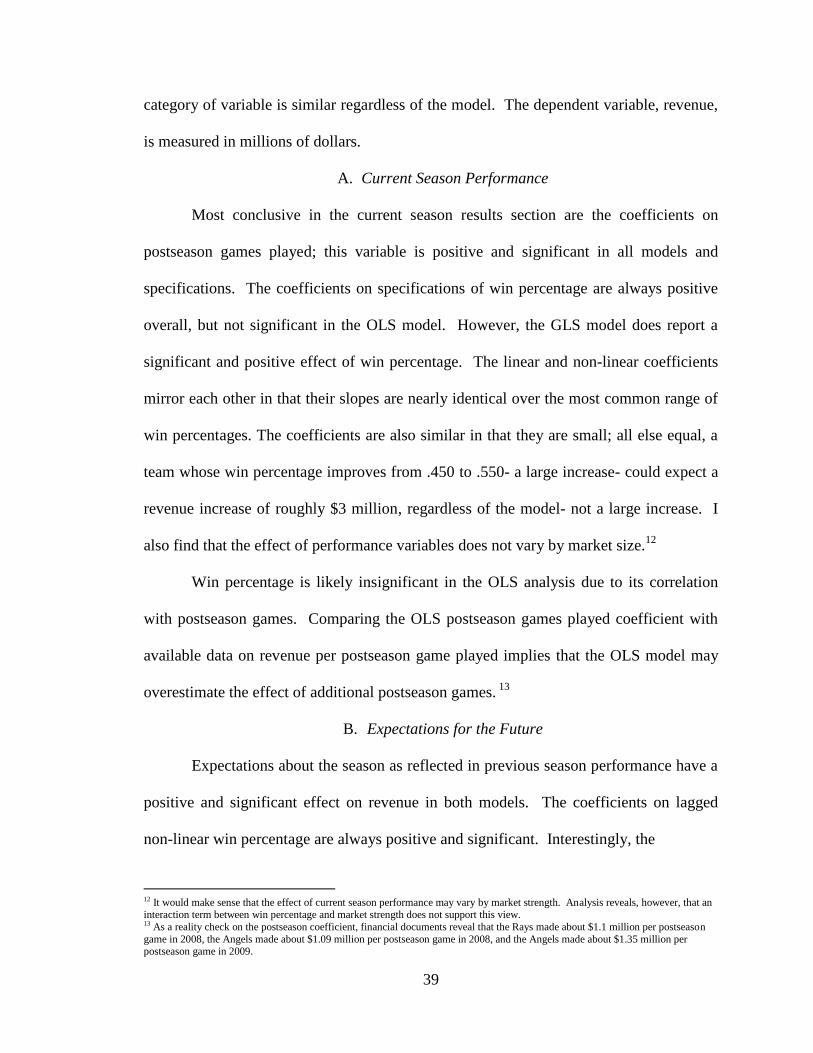
39

category of variable is similar regardless of the model. The dependent variable, revenue,

is measured in millions of dollars.

A. Current Season Performance

Most conclusive in the current season results section are the coefficients on

postseason games played; this variable is positive and significant in all models and

specifications. The coefficients on specifications of win percentage are always positive

overall, but not significant in the OLS model. However, the GLS model does report a

significant and positive effect of win percentage. The linear and non-linear coefficients

mirror each other in that their slopes are nearly identical over the most common range of

win percentages. The coefficients are also similar in that they are small; all else equal, a

team whose win percentage improves from .450 to .550- a large increase- could expect a

revenue increase of roughly $3 million, regardless of the model- not a large increase. I

also find that the effect of performance variables does not vary by market size.12

Win percentage is likely insignificant in the OLS analysis due to its correlation

with postseason games. Comparing the OLS postseason games played coefficient with

available data on revenue per postseason game played implies that the OLS model may

overestimate the effect of additional postseason games. 13

B. Expectations for the Future

Expectations about the season as reflected in previous season performance have a

positive and significant effect on revenue in both models. The coefficients on lagged

non-linear win percentage are always positive and significant. Interestingly, the

12 It would make sense that the effect of current season performance may vary by market strength. Analysis reveals, however, that an interaction term between win percentage and market strength does not support this view. 13 As a reality check on the postseason coefficient, financial documents reveal that the Rays made about $1.1 million per postseason

game in 2008, the Angels made about $1.09 million per postseason game in 2008, and the Angels made about $1.35 million per postseason game in 2009.

40

Table 5.1: Regression Results

OLS GLS

(1) (2) (3) (4) (5) (6)

CATEGORY VARIABLES revenue revenue revenue revenue revenue revenue

Current Season

Performance

Top Quintile

Interaction

7.367

2.964

(6.882)

(5.493)

Second Quintile

Interaction

4.604

3.952

(6.503)

(4.099)

Third Quintile

Interaction

-3.825

2.603

(5.635)

(3.114)

Fourth Quintile

Interaction

5.390

4.214

(5.216)

(2.835)

Linear Win Percentage

20.97 8.089

25.58*** 17.74

(18.81) (24.77)

(8.932) (17.15)

Non-linear Win

Percentage

9.290

11.32***

(8.155)

(3.929)

Postseason Games 1.413*** 1.298*** 1.412*** 0.919*** 0.950*** 0.918***

(0.382) (0.422) (0.386) (0.141) (0.152) (0.141)

Expectations for

the Future

Lag Non-linear Win

Percent

20.96*** 20.08** 20.97*** 9.311** 9.315** 9.467**

(7.474) (7.488) (7.424) (3.943) (3.967) (3.959)

Lag Postseason Games -0.0419 -0.0350 -0.0426 0.00586 0.00545 0.00197

(0.605) (0.608) (0.606) (0.144) (0.144) (0.145)

Historical

Performance

Trips to Postseason in

10 Years

-1.630 -1.484 -1.617 2.425 2.185 2.453

(2.817) (2.854) (2.818) (2.164) (2.184) (2.164)

Years in City -0.0614 -0.0751 -0.0610 -0.0233 -0.0194 -0.0227

(0.102) (0.0995) (0.102) (0.0780) (0.0781) (0.0780)

Postseason Trips x

Years

0.0904 0.0909* 0.0902 -0.00184 -0.00114 -0.00209

(0.0535) (0.0529) (0.0535) (0.0279) (0.0280) (0.0279)

Postseason Trips x

Aggregate Inc.

1.31e-11* 1.29e-11* 1.31e-11* 1.50e-11*** 1.53e-11*** 1.50e-11***

(7.00e-11) (6.92e-12) (6.99e-12) (5.72e-12) (5.74e-12) (5.72e-12)

Other

Characteristics

Strike Season -24.41*** -22.98*** -24.44*** -6.866 -6.209 -6.858

(6.031) (6.092) (6.029) (7.949) (7.984) (7.948)

First Year Expansion

Team

40.61*** 39.54*** 40.67*** -9.640 -8.846 -9.663

(12.65) (11.87) (12.65) (7.843) (7.860) (7.841)

Stadium Quality Non-linear Stadium

Age

44.54*** 44.36*** 44.52*** 39.69*** 39.68*** 39.65***

(8.101) (7.913) (8.104) (3.222) (3.235) (3.222)

Market

Characteristics

Pro Teams in DMA -4.423 -4.555 -4.425 -3.534 -3.442 -3.493

(4.051) (4.043) (4.055) (2.616) (2.622) (2.616)

MSA Unemployment -0.422 -0.461 -0.419 -1.582 -1.624 -1.580

(2.012) (1.967) (2.014) (1.217) (1.226) (1.217)

Aggregate Income

Data

3.45e-10* 3.62e-10* 3.45e-10* 1.50e-09*** 1.51e-09*** 1.50e-09***

(1.80e-10) (1.86e-10) (1.80e-10) (3.22e-10) (3.24e-10) (3.22e-10)

TV Households in

DMA

2.11e-05 1.91e-05 2.11e-05 -3.65e-06 -4.21e-06 -3.49e-06

(1.86e-05) (1.93e-05) (1.86e-05) (1.28e-05) (1.29e-05) (1.28e-05)

DMA Businesses 0.000168*** 0.000167*** 0.000168*** 5.20e-05 5.02e-05 5.17e-05

(3.47e-05) (3.36e-05) (3.48e-05) (3.70e-05) (3.71e-05) (3.69e-05)

Percent over 65 -576.6 -558.5 -575.6 -887.2 -903.3 -883.1

(579.3) (577.9) (578.9) (549.2) (551.3) (549.2)

Percent African

American

-132.1 -131.2 -131.9 -236.2* -241.4* -235.8*

(108.1) (107.3) (108.0) (140.6) (141.2) (140.6)

Percent Hispanic -118.3 -118.1 -118.3 -83.34 -80.32 -82.16

(143.4) (141.1) (143.7) (231.9) (233.4) (231.8)

Constant

-13.02 -7.258 -7.323 -20.25 -15.18 -13.83

(79.53) (78.79) (80.69) (16.48) (16.46) (16.46)

Observations 578 578 578 548 548 548

R-squared 0.883 0.884 0.883

Number of t_id 30 30 30 30 30 30

Robust standard errors in parentheses

*** p<0.01, ** p<0.05, * p<0.1

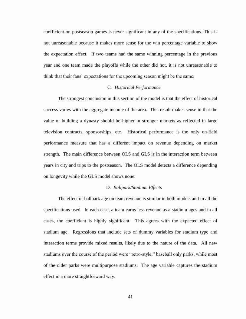
41

coefficient on postseason games is never significant in any of the specifications. This is

not unreasonable because it makes more sense for the win percentage variable to show

the expectation effect. If two teams had the same winning percentage in the previous

year and one team made the playoffs while the other did not, it is not unreasonable to

think that their fans‟ expectations for the upcoming season might be the same.

C. Historical Performance

The strongest conclusion in this section of the model is that the effect of historical

success varies with the aggregate income of the area. This result makes sense in that the

value of building a dynasty should be higher in stronger markets as reflected in large

television contracts, sponsorships, etc. Historical performance is the only on-field

performance measure that has a different impact on revenue depending on market

strength. The main difference between OLS and GLS is in the interaction term between

years in city and trips to the postseason. The OLS model detects a difference depending

on longevity while the GLS model shows none.

D. Ballpark/Stadium Effects

The effect of ballpark age on team revenue is similar in both models and in all the

specifications used. In each case, a team earns less revenue as a stadium ages and in all

cases, the coefficient is highly significant. This agrees with the expected effect of

stadium age. Regressions that include sets of dummy variables for stadium type and

interaction terms provide mixed results, likely due to the nature of the data. All new

stadiums over the course of the period were “retro-style,” baseball only parks, while most

of the older parks were multipurpose stadiums. The age variable captures the stadium

effect in a more straightforward way.

42

E. Strike Seasons/Expansion Season

The OLS regressions capture the expected effects of both strike seasons and

expansion years. Unfortunately, however, the GLS model does not support these

conclusions as both strike season and expansion year are not significant in the model.

F. Market Strength

The OLS and GLS models show a similar overall impact of the variables in this

category. In both models, aggregate income is positive and statistically significant.

Furthermore, the coefficient on businesses was highly significant in the OLS models, but

loses significance in the GLS models likely due to correlation with aggregate income and

other economic variables. The TV Households variable is never significant, likely due to

correlation with aggregate income and number of businesses.

In both models, both the number of professional sports teams in the DMA and the

MSA unemployment rates have the anticipated sign, but they are not statistically

significant. The coefficient on percent African American is not significant in the OLS

model, but its coefficient nearly doubles in absolute value and becomes significant at the

10% level in the GLS regressions. The coefficients on percent over 65 have the

anticipated sign, but are not statistically significant. The coefficient on percent Hispanic

is also not statistically significant. The results of this section are broadly consistent in

that measures of market strength are important regardless of the choice of model.

5.5 A New Sharing System

In 2006, MLB began to correct perverse incentives by relying on “performance

factors.”14

However, this system still bases revenue sharing on actual revenue and it

14 See the previous chapter for a more detailed description of performance factors.

43

penalizes well managed teams to reward more poorly managed ones. Kesenne (2004)

writes of his distinction between “good” and “bad imbalance that:

Moreover, almost everybody agrees that something should be done about

a bad imbalance that gets out of hand, whereas there can be serious doubt

that a good competitive imbalance should be “cured” and possibly turned

into a bad one. Revenue sharing based on a club‟s market size instead of

on its budget is a possible way out. (Kesenne 2004, 211)

The 2006 sharing system was designed in a way that could “cure” a good imbalance and

turn it into a “bad” one. I use the results of the preceding analysis to show the ways in

which the 2006 sharing plan risks curing a “good” imbalance in favor of a “bad” one.

In table 5.2, I present the following:

(1) “Actual” revenue by team for 200915

(2) Predicted revenue based on the model in 5.4 and actual team performance in

200916

(3) 2009 market strength value generated with the model by assuming average

performance for all teams. (e.g. .500 winning percentage, no postseason, etc)

(4) Market strength values generated with the model by assuming average

performance for all teams; for comparison with 2006 CBA revenue data; ranks17

(5) Revenue figures used by the 2006 CBA to determine sharing reallocation; ranks

Comparing “actual” revenue for 2009 (1) and predicted revenue18

for 2009 (2), shows

that the model underestimates high revenue clubs and overestimates low revenue clubs.

Column (3) reports estimated market strength for each team in 2009.

15 These data are estimated in the fashion discussed in section 5.1. 16 The “Predicted Revenue” values are the average of the predictions made by the three OLS models given market characteristics and

actual team performance for 2009. 17 The “Predicted 2006 Revenue” is an average of the predicted revenue for each team across the three OLS models, over the four

seasons 2004-2007 while assuming average performance. These values are computed in the same fashion as the CBA values were,

but they assume equal performance on the field and are thus a better measure of “market strength.” 18 All “predicted revenue” values are the average values given by the three OLS specifications.

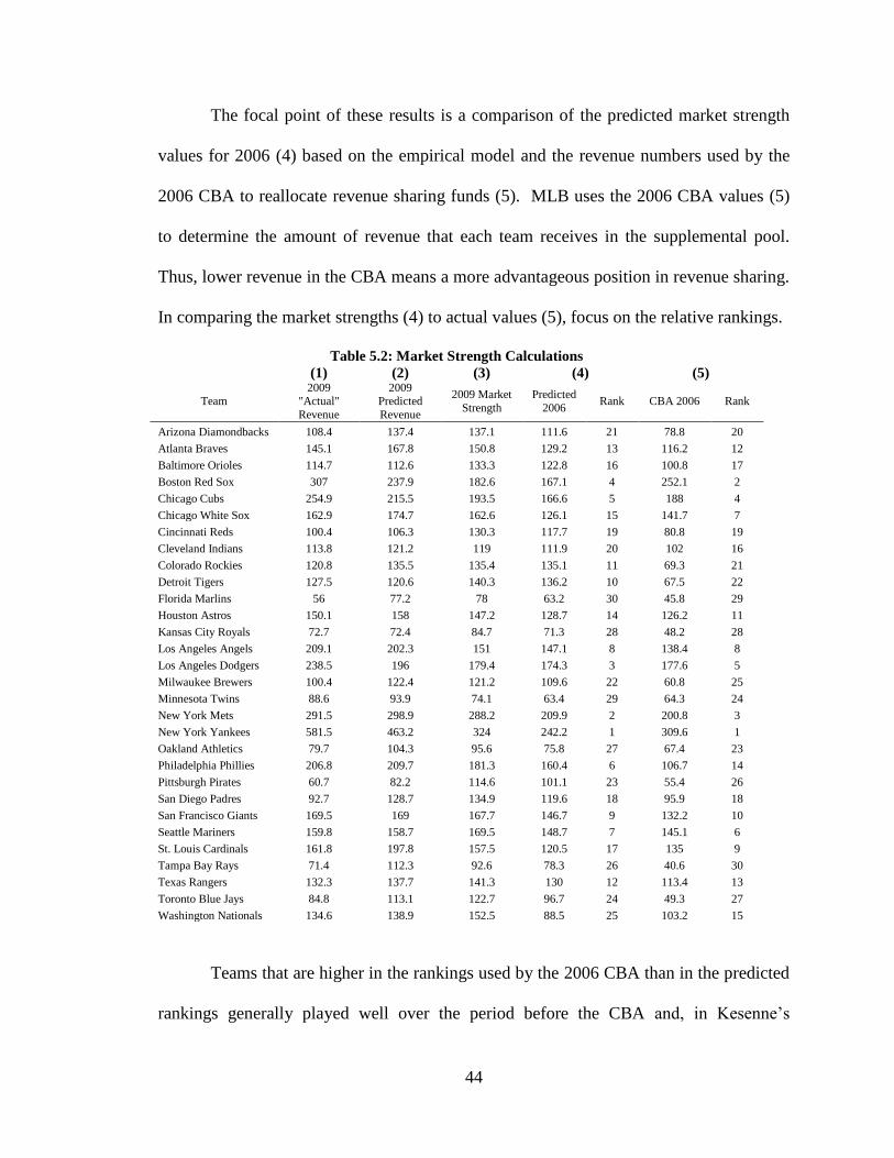
44

The focal point of these results is a comparison of the predicted market strength

values for 2006 (4) based on the empirical model and the revenue numbers used by the

2006 CBA to reallocate revenue sharing funds (5). MLB uses the 2006 CBA values (5)

to determine the amount of revenue that each team receives in the supplemental pool.

Thus, lower revenue in the CBA means a more advantageous position in revenue sharing.

In comparing the market strengths (4) to actual values (5), focus on the relative rankings.

Table 5.2: Market Strength Calculations

(1) (2) (3) (4) (5)

Team 2009

"Actual"

Revenue

2009 Predicted

Revenue

2009 Market

Strength

Predicted

2006 Rank CBA 2006 Rank

Arizona Diamondbacks 108.4 137.4 137.1 111.6 21 78.8 20

Atlanta Braves 145.1 167.8 150.8 129.2 13 116.2 12

Baltimore Orioles 114.7 112.6 133.3 122.8 16 100.8 17

Boston Red Sox 307 237.9 182.6 167.1 4 252.1 2

Chicago Cubs 254.9 215.5 193.5 166.6 5 188 4

Chicago White Sox 162.9 174.7 162.6 126.1 15 141.7 7

Cincinnati Reds 100.4 106.3 130.3 117.7 19 80.8 19

Cleveland Indians 113.8 121.2 119 111.9 20 102 16

Colorado Rockies 120.8 135.5 135.4 135.1 11 69.3 21

Detroit Tigers 127.5 120.6 140.3 136.2 10 67.5 22

Florida Marlins 56 77.2 78 63.2 30 45.8 29

Houston Astros 150.1 158 147.2 128.7 14 126.2 11

Kansas City Royals 72.7 72.4 84.7 71.3 28 48.2 28

Los Angeles Angels 209.1 202.3 151 147.1 8 138.4 8

Los Angeles Dodgers 238.5 196 179.4 174.3 3 177.6 5

Milwaukee Brewers 100.4 122.4 121.2 109.6 22 60.8 25

Minnesota Twins 88.6 93.9 74.1 63.4 29 64.3 24

New York Mets 291.5 298.9 288.2 209.9 2 200.8 3

New York Yankees 581.5 463.2 324 242.2 1 309.6 1

Oakland Athletics 79.7 104.3 95.6 75.8 27 67.4 23

Philadelphia Phillies 206.8 209.7 181.3 160.4 6 106.7 14

Pittsburgh Pirates 60.7 82.2 114.6 101.1 23 55.4 26

San Diego Padres 92.7 128.7 134.9 119.6 18 95.9 18

San Francisco Giants 169.5 169 167.7 146.7 9 132.2 10

Seattle Mariners 159.8 158.7 169.5 148.7 7 145.1 6

St. Louis Cardinals 161.8 197.8 157.5 120.5 17 135 9

Tampa Bay Rays 71.4 112.3 92.6 78.3 26 40.6 30

Texas Rangers 132.3 137.7 141.3 130 12 113.4 13

Toronto Blue Jays 84.8 113.1 122.7 96.7 24 49.3 27

Washington Nationals 134.6 138.9 152.5 88.5 25 103.2 15

Teams that are higher in the rankings used by the 2006 CBA than in the predicted

rankings generally played well over the period before the CBA and, in Kesenne‟s

45

language, could be said to contribute “good” imbalance.19

MLB penalized these teams

because it computed the values in column (5) based on revenues that captured the teams‟

“over-achievement.” Conversely, teams ranked higher in the predicted revenue ranking

enjoyed the financial benefits in revenue sharing of poor performance before the CBA

was signed. MLB risks creating a “bad” imbalance by supporting underachieving large

market teams in revenue sharing. For instance, the Philadelphia Phillies received revenue

in the system implemented by MLB, yet they play in a strong market (ranked 6th

in my

index). Their performance on the field before 2006 had been mediocre at best and

inspired little excitement from their fans. Thus, the team‟s revenues lagged and by using

these seasons as the basis for revenue sharing, MLB continues to distribute money to the

Phillies as though they are a small market team. Despite leading the National League in

attendance in 2010, the Phillies still were net recipients in the supplemental pool.20

The 2006 CBA began to alleviate the incentive problems in revenue sharing, but it

still left the problem of subsidization of under-achieving large market teams. A new

system based upon a measure of underlying market strength like that calculated in

columns (3) and (4) will eliminate the risks of turning “good” competitive imbalance into

“bad” competitive imbalance. This system will introduce marginal tax rates of zero that

will increase player salaries and promote growth an innovation among owners. Owners

will find some investments profitable under this system that they did not in previous

systems. However, because there are no redistributive effects, this system will not

improve balance beyond the level prevailing in competition. This system will return

team incentives to the competitive solution without sharing. In this way, if the league

19 This is to say that they earned more than their market strength indicates had every team been equally talented. The Nationals are the

exception. A comparison of their values is problematic because the team moved cities in 2005. 20 Because the sharing plan also incorporates a portion based on actual current season revenue, the team would not have been a net recipient overall in the sharing system, but they would have in the portion that was predetermined by the CBA.

46

seeks to improve balance, it must explore other options such as salary caps (and floors),

luxury taxes, progressive payroll taxes, and the like.

5.6 The Effect of Revenue Sharing on Balance in MLB

The justification for revenue sharing is that differential market potential leads to

differential payroll potential which leads to differential performance potential. To

examine whether MLB‟s revenue sharing systems had an effect on the distribution of

talent, I examine changes in the payroll distribution. The idea is that market strength is

correlated with payroll, but that the revenue sharing institutions changed this relationship.

I construct a model to test this proposition by creating a new set of variables.

End of Season Payroll Proportion: the proportion of total end of season

league payroll attributable to a particular team

Market Strength Proportion: market strength developed with the model as

a proportion of the total market strength for the league.21

CBA Dummies: dummy variable each for the 1996, 2002, and 2006 CBA

CBA Interactions: interaction between market strength proportion and

each CBA dummy variable

I estimate the following regression:

If the coefficients on the interaction terms are significant, then we can conclude that the

relationship between market strength and payroll proportion has changed. More

21 The market strength index is calculated in the same manner as in column (3) of table 5.2. I calculate this index for each season.

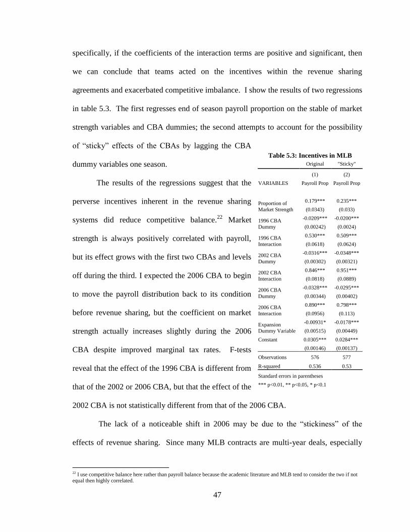
47

specifically, if the coefficients of the interaction terms are positive and significant, then

we can conclude that teams acted on the incentives within the revenue sharing

agreements and exacerbated competitive imbalance. I show the results of two regressions

in table 5.3. The first regresses end of season payroll proportion on the stable of market

strength variables and CBA dummies; the second attempts to account for the possibility

of “sticky” effects of the CBAs by lagging the CBA

dummy variables one season.

The results of the regressions suggest that the

perverse incentives inherent in the revenue sharing

systems did reduce competitive balance.22

Market

strength is always positively correlated with payroll,

but its effect grows with the first two CBAs and levels

off during the third. I expected the 2006 CBA to begin

to move the payroll distribution back to its condition

before revenue sharing, but the coefficient on market

strength actually increases slightly during the 2006

CBA despite improved marginal tax rates. F-tests

reveal that the effect of the 1996 CBA is different from

that of the 2002 or 2006 CBA, but that the effect of the

2002 CBA is not statistically different from that of the 2006 CBA.

The lack of a noticeable shift in 2006 may be due to the “stickiness” of the

effects of revenue sharing. Since many MLB contracts are multi-year deals, especially

22 I use competitive balance here rather than payroll balance because the academic literature and MLB tend to consider the two if not equal then highly correlated.

Table 5.3: Incentives in MLB

Original "Sticky"

(1) (2)

VARIABLES Payroll Prop Payroll Prop

Proportion of

Market Strength

0.179*** 0.235***

(0.0343) (0.033)

1996 CBA

Dummy

-0.0209*** -0.0200***

(0.00242) (0.0024)

1996 CBA

Interaction

0.530*** 0.509***

(0.0618) (0.0624)

2002 CBA

Dummy

-0.0316*** -0.0348***

(0.00302) (0.00321)

2002 CBA

Interaction

0.846*** 0.951***

(0.0818) (0.0889)

2006 CBA

Dummy

-0.0328*** -0.0295***

(0.00344) (0.00402)

2006 CBA

Interaction

0.890*** 0.798***

(0.0956) (0.113)

Expansion

Dummy Variable

-0.00931* -0.0178***

(0.00515) (0.00449)

Constant 0.0305*** 0.0284***

(0.00146) (0.00137)

Observations 576 577

R-squared 0.536 0.53

Standard errors in parentheses

*** p<0.01, ** p<0.05, * p<0.1

48

more lucrative contracts, I expect the effects of a CBA to linger longer than the life of the

CBA. Thus, contracts signed during the 2002 CBA may still be on the books of teams

during the 2006 CBA. For this reason, I include regression 2 that crudely accounts for

this issue by lagging the CBA variables.23

The coefficient on the 2006 CBA interaction

falls slightly, but an F-test does not reveal a statistically significant change. The

difference when including the CBA lags indicates that the 2006 CBA may have begun to

realign incentives, but that it will take more time before older contracts expire.

6 Conclusion

In this paper, I have examined competitive balance, revenue sharing, and their

relationship. I developed a theoretical model of revenue sharing. In this model, I posited

a three-team case that demonstrates that when a team‟s marginal private cost of talent

does not equal its marginal social cost of talent, revenue sharing can affect balance.

Following the theoretical treatment, I explicated the history of luxury taxes and

revenue sharing in MLB. Despite a stated commitment to promoting competitive

balance, the institutions put in place by MLB in the 1996 and 2002 agreements created

perverse incentives such that small market teams faced higher marginal tax rates than

large market teams. Realizing this mistake, the 2006 CBA alleviates this problem, but

risks “curing” good imbalance and replacing it with bad imbalance.

In section 5, I develop an empirical model of revenue generation in MLB. In this

section, I provide empirical support to the notion that the 2006 CBA risks converting

good imbalances into bad ones. I propose a system of revenue sharing based upon

23 The regression assumes that the 1996 CBA operated from 1997-2003, the 2002 CBA from 2004-2007, and the 2006 CBA from 2008 onwards.

49

market strength that avoids this problem. I then use the results of the model to

demonstrate two important conclusions about MLB revenue sharing:

(1) The 1996 and 2002 CBAs adversely affected competitive balance commensurate

with their perverse incentives.

(2) The 2006 CBA has not yet conclusively demonstrated effects on balance that

differ from the 2002 CBA, but initial evidence suggests that it may be moving

balance back toward the pre-revenue sharing levels.

The analysis also indicates that the effects of these systems are sticky; although MLB has

begun to fix the problems, it will likely take more time for the improvements to take hold.

Regardless, however, this research shows that MLB has tried many times and

ultimately appears to have failed in their attempts to promote competitive balance

through increased payroll balance. They have failed because they have constructed

institutions that create backwards incentives and because they have failed to draw a

distinction between “good” and “bad” imbalance. New sharing systems in MLB should

account for these past failings and allocate resources in a new way that will incentivize

success, not subsidize failure.

REFERENCES

Atkinson, Scott E., Linda R. Stanley, and John Tschirhart. "Revenue Sharing as an

Incentive in an Agency Problem: an Example from the National Football League." RAND

Journal of Economics, 1988: 27-43.

Canes, Michael R. "The Social Benefits of Restrictions on Team Quality." In

Government and the Sports Business, by ed. Roger Noll, 81-113. Washington, DC: The

Brookings Institution, 1974.

El-Hodiri, Mohamed, and James Quirk. "An Economic Model of a Professional Sports

League." Journal of Political Economy, 1971: 1302-1319.

Fort, Rodney, and James Quirk. "Cross-Subsidization, Incentives, and Outcomes in

Professional Team Sports Leagues." Journal of Economic Literature, 1995: 1265-1299.

50

Fort, Rodney, and James Quirk. "Optimal Competitive Balance in Single-Game Ticket

Sports Leagues." Journal of Sports Economics, 2010: 587-601.

Hall, Stephen, Stefan Szymanski, and Andrew Zimbalist. "Testing the Causality Between

Team Performance and Payroll." Journal of Sports Economics, 2002: 149-168.

Humphreys, Brad. "Alternative Measures of Competitive Balance in Sports Leagues."

Journal of Sports Economics, 2002: 133-148.

Kesenne, Stefan. "Competitive Balance and Revenue Sharing: When Rich Clubs Have

Poor Teams." Journal of Sports Economics, 2004: 206-212.

Kesenne, Stefan. "Revenue Sharing and Competitive Balance in Professional Team

Sports." Journal of Sports Economics, 2000: 56-65.

Lee, Young Hoon, and Rodney Fort. "Attendance and teh Uncertainty-of-Outcome

Hypothesis in Baseball." Review of Industrial Organization, 2008: 281-295.

Levin, Richard C., George J. Mitchell, Paul A. Volcker, and George F. Will. The Report

of the Independent Members of the Commissioner's Blue Ribbon Panel on Baseball

Economics. Major League Baseball, 2000.

Marburger, Daniel R. "Gate Revenue Sharing and Luxury Taxes in Professional Sports."

Contemporary Economic Policy, 1997: 114-123.

Maxcy, Joel G. "Progressive Revenue Sharing in Major League Baseball: The Effects on

Player Transfers and Talent Distribution." Review of Industrial Organization, 2009: 275-

297.

Meehan Jr., James W., Randy A. Nelson, and Thomas V. Richardson. "Competitive

Balance and Game Attendance in Major League Baseball." Journal of Sports Economics,

2007: 563-580.

Neale, Walter C. "The Peculiar Economics of Professional Sports." The Quarterly

Journal of Economics, 1964: 1-14.

Noll, Roger G. "Attendance and Price Setting." In Government and the Sports Business,

by Roger G. Noll, 115-157. Washington, DC: The Brookings Institution, 1974.

Quirk, James, and Rodney Fort. Hard Ball. Princeton, NJ: Princeton University Press,

1999.

—. Pay Dirt. Princeton, NJ: Princeton University Press, 1992.

Rottenberg, Simon. "The Baseball Players' Labor Market." The Journal of Political

Economy, 1956: 242-258.

Szymanski, Stefan. "The Economic Design of Sporting Contests." Journal of Economic

Literature, 2003: 1137-1187.

Szymanski, Stefan, and Andrew Zimbalist. National Pastime. Washington, DC:

Brookings Institution Press, 2005.

Szymanski, Stefan, and Stefan Kesenne. "Competitive Balance and Gate Revenue

Sharing in Team Sports." The Journal of Industrial Economics, 2004: 165-177.

51

Vrooman, John. "Theory of the Perfect Game: Competitive Balance in Monopoly Sports

Leagues." Review of Industrial Organization, 2009: 5-44.

Zimbalist, Andrew. "Competitive Balance in Sports Leagues." Journal of Sports

Economics, 2002: 111-120.

—. May the Best Team Win. Washington, D.C.: Brookings Institution Press, 2003.