Review of basic quantum Review of basic quantum and Deutsch-Jozsa.and Deutsch-Jozsa.

Can we generalize Deutsch-Jozsa algorithm?

Marek Perkowski, Department of Electrical Engineering, Portland State University, 2005

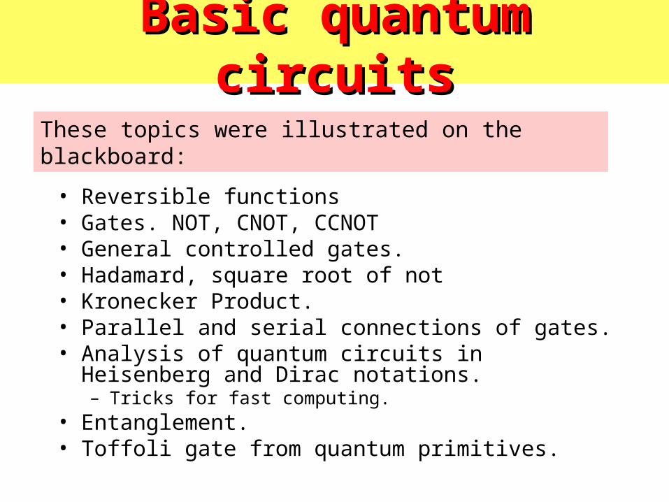
Basic quantum circuitsBasic quantum circuits

• Reversible functions• Gates. NOT, CNOT, CCNOT• General controlled gates.• Hadamard, square root of not• Kronecker Product.• Parallel and serial connections of gates.• Analysis of quantum circuits in Heisenberg and Dirac

notations.– Tricks for fast computing.

• Entanglement.• Toffoli gate from quantum primitives.

These topics were illustrated on the blackboard:

Deutsch’s Deutsch’s ProblemProblem

… everything started with small circuit of Deutsch…...

Deutsch’s Problem

David Deutsch

Delphi

Deutsch’s ProblemDeutsch’s ProblemDetermine whether f(x) is constant or balanced using as few queries to the oracle as possible.

(1985)(Deutsch ’85)

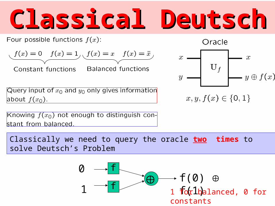
Classical DeutschClassical Deutsch

Classically we need to query the oracle two times to solve Deutsch’s Problem

f

ff(0) f(1)

1 for balanced, 0 for constants

0

1

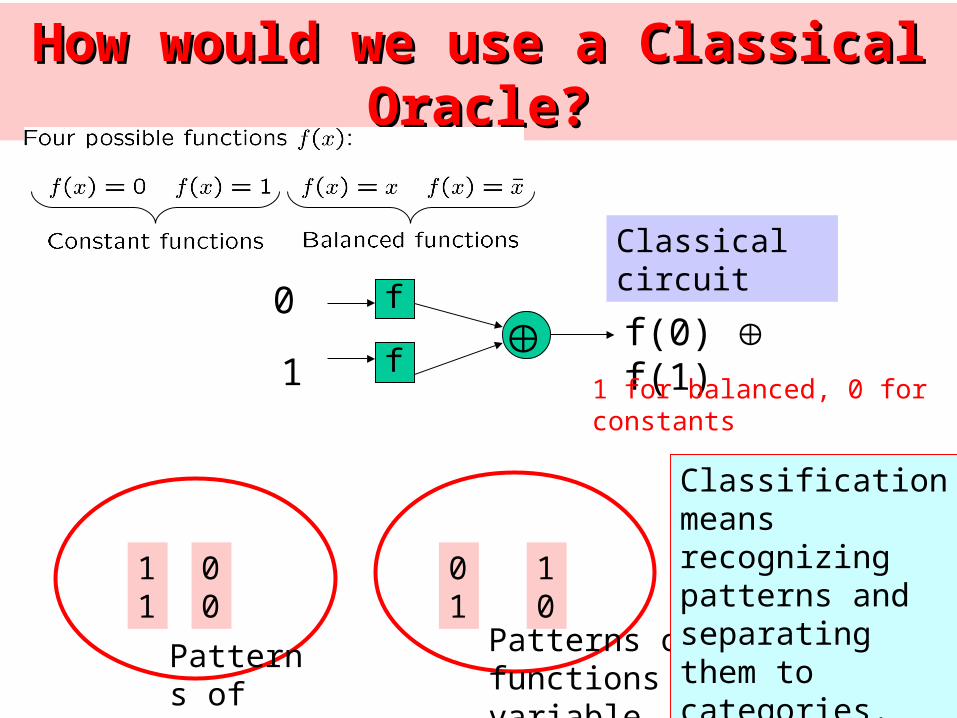
How would we use a Classical How would we use a Classical Oracle?Oracle?

f

ff(0) f(1)

1 for balanced, 0 for constants

0

1

1 1

0 0

0 1

1 0

Patterns of constants

Patterns of balanced functions of single variable

Classical circuit

Classification means recognizing patterns and separating them to categories.

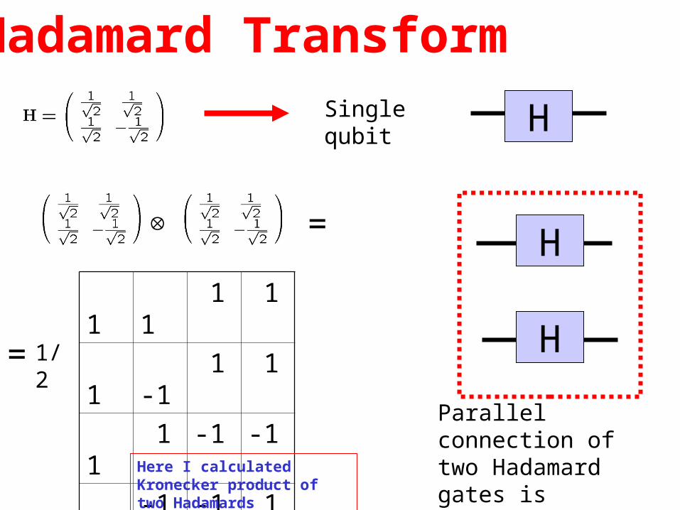
Hadamard TransformSingle qubit H

H

H

Parallel connection of two Hadamard gates is calculated by Kronecker Product (tensor product)

1 1 1 1

1 -1 1 1

1 1 -1 -1

1 -1 -1 1

1/2

=

=

Here I calculated Kronecker product of two Hadamards

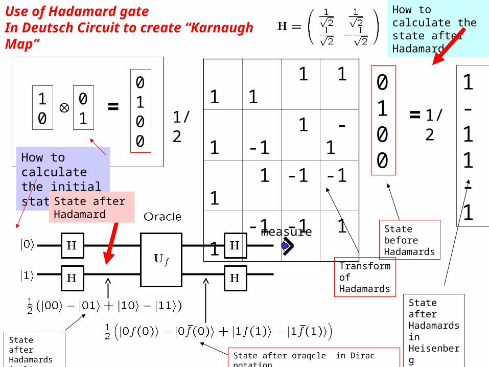
Use of Hadamard gateIn Deutsch Circuit to create “Karnaugh Map”

measure

1 0

0 1

01 00

=

1 1 1 1

1 -1 1 -1

1 1 -1 -1

1 -1 -1 1

1/2

01 00

= 1/2

1 -1 1 -1

How to calculate the state after Hadamard

How to calculate the initial state

State after Hadamard

State before Hadamards

Transform of Hadamards

State after Hadamards in Heisenberg notation

State after Hadamards in Dirac notation State after oraqcle in Dirac notation

RemarksRemarks

• We use both Heisenberg and Dirac notation because some things are easier to prove in Dirac and some in Heisenberg.

• You can verify everything in Heisenberg, which is easy, but takes many matrix calculations.

• Dirac notation introduces many transformations that may be not obvious, if you are in doubt, just verify in Heisenberg notation.

• Because Dirac notation introduces symbol manipulation, you can avoid repeated calculation. In next stages some standard transforms of Dirac notation will be useful, but they are useful only to prove facts, rather than invent facts.

• You can verify the state after oracle by yourself from definition, but on the next page we will show everything step-by-step. In future we will skip sometimes such obvious transformations.

Deutsch Circuit

measure

|xy>|x yf(x)>

|00> |0 0 f(0)> = |0 f(0)>

|01> |0 1f(x)> = |0 f(0)>

|10> |1 0 f(1)> = |1 f(1)>

|11> |1 1 f(1)> = |1 f(1)>

½ (|00> - |01> + |10> - |11>)

½ (|0 f(0)> - |0 f(0)> + |1 f(1)> - |1 f(1)> )

How to calculate state after oracle?

Derivation of formula from previous page

Such derivations should be done for every quantum algorithm.

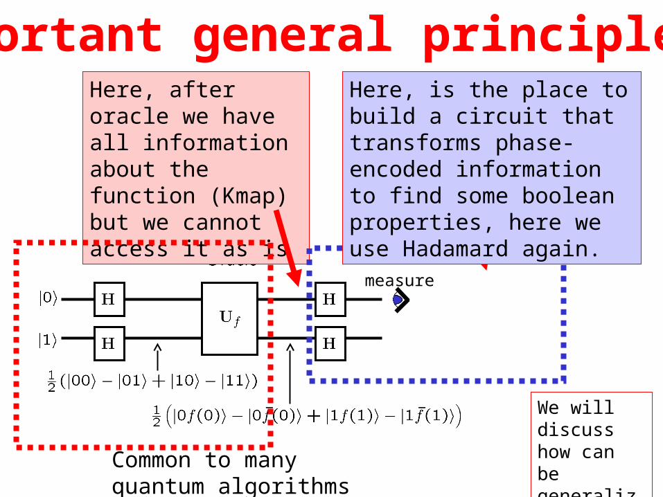
Important general principle

measure

Here, after oracle we have all information about the function (Kmap) but we cannot access it as is

Common to many quantum algorithms

Here, is the place to build a circuit that transforms phase-encoded information to find some boolean properties, here we use Hadamard again.

We will discuss how can be generalized!

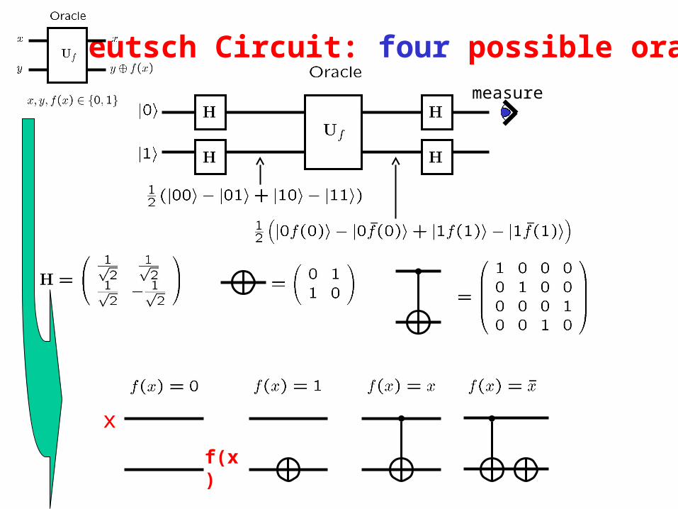
Deutsch Circuit: four possible oraclesmeasure

x

f(x)

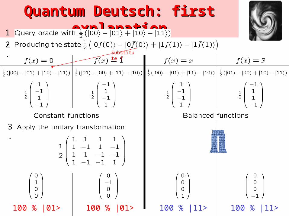
Quantum Deutsch: first Quantum Deutsch: first explanationexplanation1.

2.

3.

100 % |01> 100 % |01> 100 % |11> 100 % |11>

Substitute f

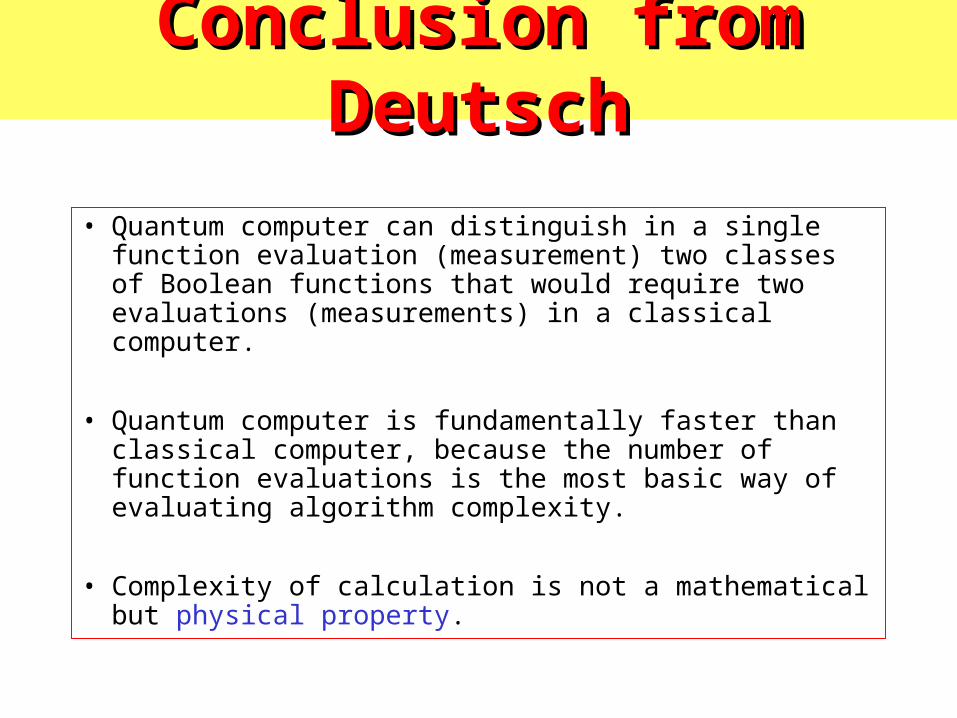
Conclusion from DeutschConclusion from Deutsch

• Quantum computer can distinguish in a single function evaluation (measurement) two classes of Boolean functions that would require two evaluations (measurements) in a classical computer.

• Quantum computer is fundamentally faster than classical computer, because the number of function evaluations is the most basic way of evaluating algorithm complexity.

• Complexity of calculation is not a mathematical but physical property.

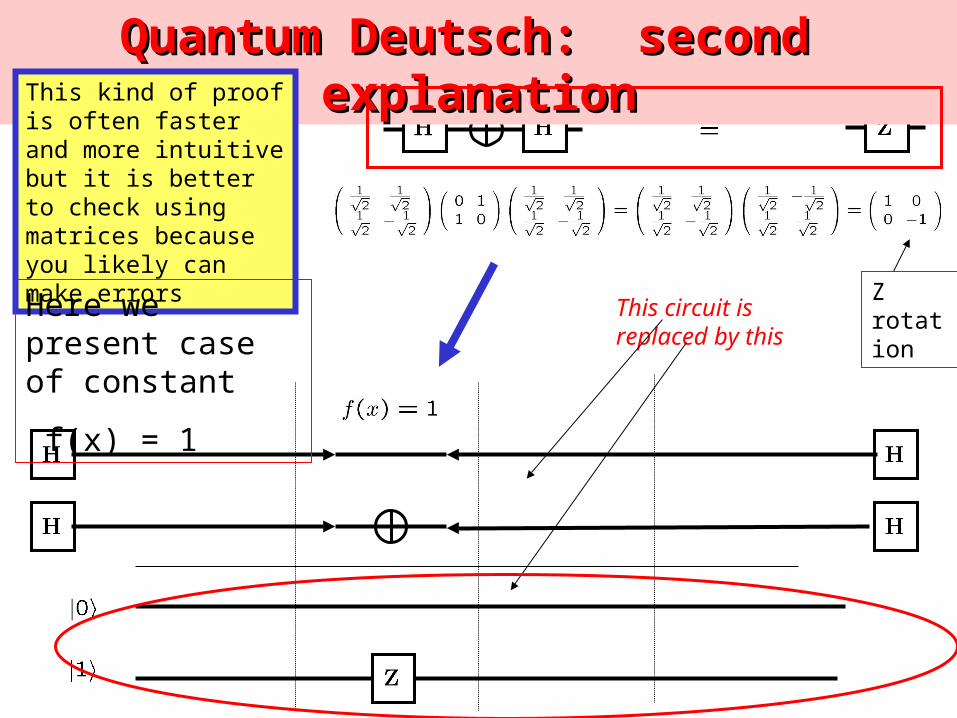
Quantum Deutsch: second Quantum Deutsch: second explanationexplanationThis kind of proof is often

faster and more intuitive but it is better to check using matrices because you likely can make errors

This circuit is replaced by this

Here we present case of constant

f(x) = 1

Z rotation

Quantum Deutsch: second Quantum Deutsch: second explanationexplanation

This is obtained after connecting Hadamards and simplifying

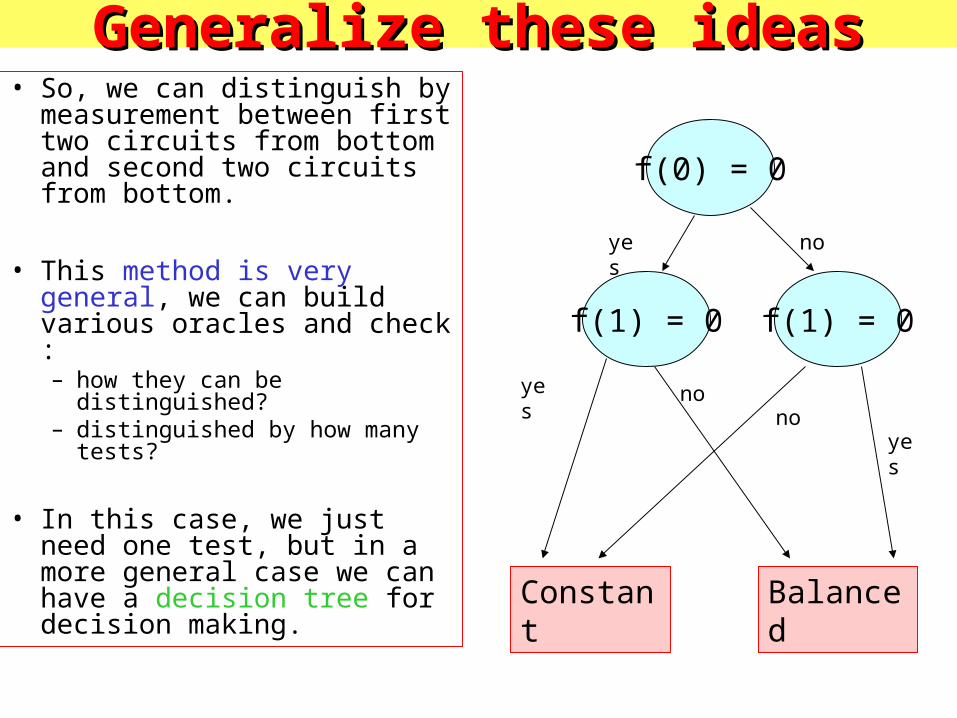
Generalize these ideasGeneralize these ideas• So, we can distinguish by

measurement between first two circuits from bottom and second two circuits from bottom.

• This method is very general, we can build various oracles and check :– how they can be distinguished?– distinguished by how many tests?

• In this case, we just need one test, but in a more general case we can have a decision tree for decision making.

f(0) = 0

f(1) = 0 f(1) = 0

yes no

yes no

yesno

Constant Balanced

Find using only 1 evaluation of a reversible “black-box” circuit for

}1,0{}1,0{: f

f)1()0( ff

)x(f

x x

b )x(fb

Quantum Quantum Deutsch: Deutsch: third third explanationexplanation

|y> |y f(x)>

This method introduces the concept of phase kickback or encoding information in phase

Phase “kick-back” trickPhase “kick-back” trick

x

)x(f10

x)1( )x(f

)10(x)1(

)10()1(x)x(f

)x(f

10

)1)x(f)x(f(x)10(x

The phase depends on function f(x)

Remember that for |y>:

|0> f(x)

|1> f(x) 1

)10(x)1(

)10()1(x)x(f

)x(f

)1)x(f)x(f(x)10(x

Check for f(x)=0:

|0> - |1>

Because 0 1 = 1

Check for f(x)=1:

|1> - |0>

Because 1 1 = 0 and next (-1) (|0>-|1>)

For careful proof checkers.

In next slide we will rewrite this formulat for |x>=0 and |x>=1, since H creates all possible values of cells.

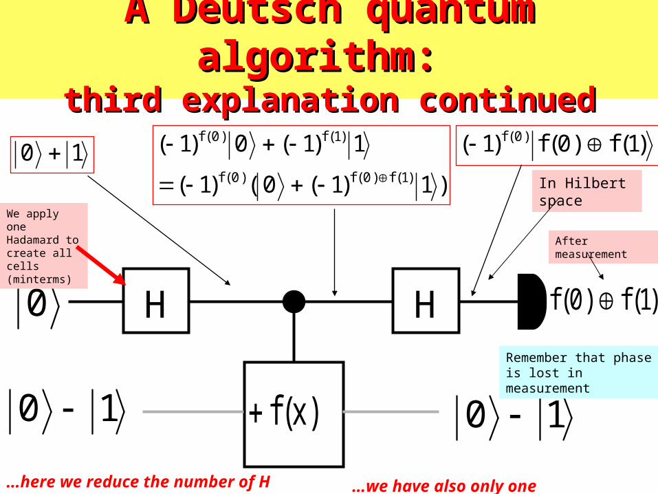
A Deutsch quantum algorithm: A Deutsch quantum algorithm: third explanation continuedthird explanation continued

0 H

)x(f

H

10 10

)1(f)0(f

10 )1)1(0()1(

1)1(0)1()1(f)0(f)0(f

)1(f)0(f

)1(f)0(f)1( )0(f

…here we reduce the number of H gates...

We apply one Hadamard to create all cells (minterms)

In Hilbert space

After measurement

…we have also only one measurement...

Remember that phase is lost in measurement

Deutsch Algorithm PhilosophyDeutsch Algorithm Philosophy Since we can prepare a superposition of all the inputs,

we can learn a global property of f (i.e. a property that depends on all the values of f(x)) by only applying f once

The global property is encoded in the phase information, which we learn via interferometryinterferometry

Classically, one application of f will only allow us to probe its value on one input

We use just one quantum evaluation by, in effect, computing f(0) and f(1) simultaneously

• The Circuit:

MH

H

H

y f(x)y

x xUf

Not always

Many variants of Deutsch algorithm can be created to provide explanation of various principles

Deutsch’s AlgorithmDeutsch’s Algorithm

MH

H

H

y f(x)y

x xUf

• Initialize with |0 = |01

|0

|1

|0

• Create superposition of x states using the first Hadamard (H) gate. Set y control input using the second H gate

|1

• Compute f(x) using the special unitary circuit Uf

|2

• Interfere the |2 states using the third H gate

|3

• Measure the x qubit

|0 = constant; |1 = balanced

measurement

M

y f(x)y

x x

Uf

|0

|1|0 |1 |2 |3

1 0 1

2

0 1

2

2 1 f (0) 0 1 f (1) 1

2

0 1

2

0 1

2

0 1

2

0 12

0 12

H

H

H

3 0 0 1

2

1 0 12

if f(0) = f(1) if f(0) ≠ f(1)

if f(0) = f(1) if f(0) ≠ f(1)

0 0 1

Deutsch’s Algorithm with single Deutsch’s Algorithm with single qubit measurementqubit measurement

Deutsch In Perspective

Quantum theory allows us to do in a single query what classically requires two queries.

What about problems where the What about problems where the computational complexity is computational complexity is exponentially exponentially more efficient?more efficient?

Balanced FunctionsBalanced Functions

1 1 1 1

1 1 1 1

1

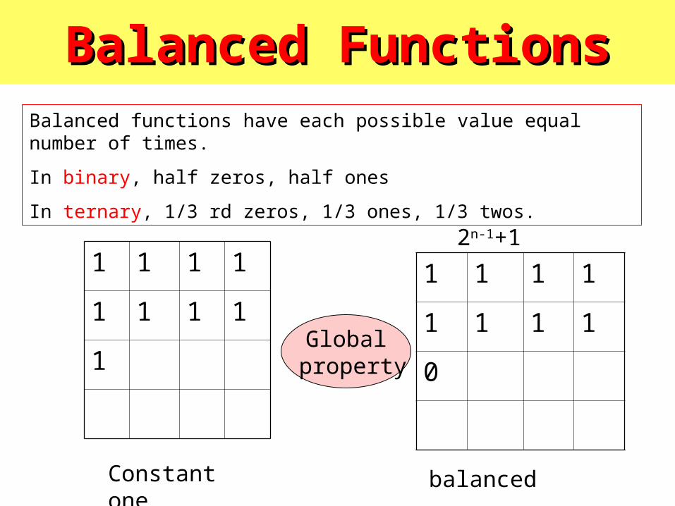
Balanced functions have each possible value equal number of times.

In binary, half zeros, half ones

In ternary, 1/3 rd zeros, 1/3 ones, 1/3 twos.

2n-1+1

1 1 1 1

1 1 1 1

0

Constant one balanced

Global property

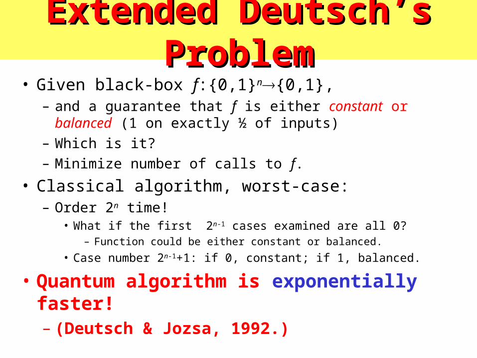
Extended Deutsch’s ProblemExtended Deutsch’s Problem• Given black-box f:{0,1}n{0,1},

– and a guarantee that f is either constant or balanced (1 on exactly ½ of inputs)

– Which is it?

– Minimize number of calls to f.

• Classical algorithm, worst-case:– Order 2n time!

• What if the first 2n-1 cases examined are all 0?– Function could be either constant or balanced.

• Case number 2n-1+1: if 0, constant; if 1, balanced.

• Quantum algorithm is exponentially faster!– (Deutsch & Jozsa, 1992.)

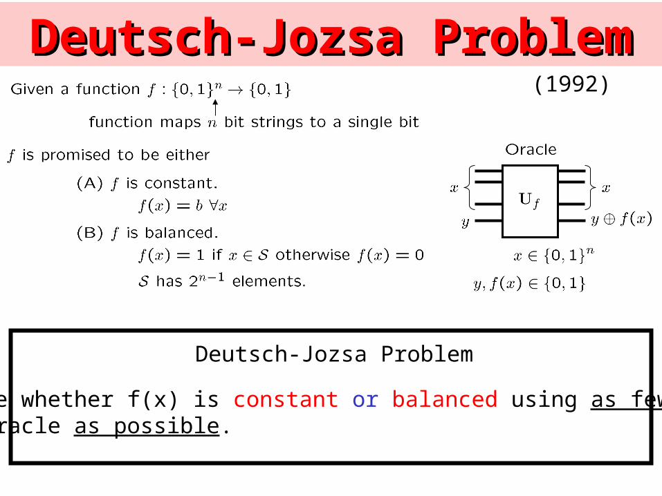
Deutsch-Jozsa ProblemDeutsch-Jozsa Problem

Deutsch-Jozsa Problem

Determine whether f(x) is constant or balanced using as few queriesto the oracle as possible.

(1992)

Classical Deutsch Jozsax

10

10 x

This slide only presents another way of visualizing constant and balanced functions.

Both visualization as a waveform (as above) and as Karnaugh Map (truth Table) have heuristic value to find analogies with signal processing and logic design

Getting good feelingGetting good feeling• Before we prove formally Deutsch-Jozsa, we

will analyze few examples for few variables, just to get intuitive feeling.

• Next we will prove the theorem formally, using Dirac notation.

• You can use Heisenberg notation as well, but it takes more space.

1. As you remember, we encode information in phase.

2. We will encode Boolean “0” using phase plus (complex number 1)

3. We will encode Boolean “1” using phase minus (complex number -1).

4. This is the so-called S encoding of spectral theory. It is better for many applications than R encoding that I do not introduce yet.

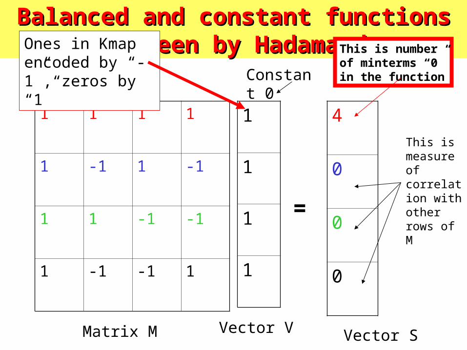
Balanced and constant functions as seen by Balanced and constant functions as seen by HadamardHadamard

1 1 1 1

1 -1 1 -1

1 1 -1 -1

1 -1 -1 1

1

1

1

1

=

4

0

0

0

Matrix M Vector V Vector S

This is number of minterms “0” in the function

This is measure of correlation with other rows of M

Constant 0

Ones in Kmap encoded by “-1”, zeros by “1”

ObservationsObservations

• The first row of the Hadamard matrix has all ones. This means that we calculate the global value corresponding to the number of ones in the first spectral parameter.

• The other than first rows of Hadamard matrix have equal number of ones and minus ones, which means that they check correlations of data vectors to certain balanced functions.

Balanced and constant functions as seen by Balanced and constant functions as seen by HadamardHadamard

1 1 1 1

1 -1 1 -1

1 1 -1 -1

1 -1 -1 1

-1

-1

-1

-1

=

- 4

0

0

0

Matrix M Vector V Vector S

This is number of minterms “1” in the function

This is measure of correlation with other rows of M

Constant 1

Balanced and constant functions as seen by Balanced and constant functions as seen by HadamardHadamard

1 1 1 1

1 -1 1 -1

1 1 -1 -1

1 -1 -1 1

1

-1

1

-1

=

0

4

0

0

Matrix M of Hadamard transform

Vector V of encoded data

Vector S of spectral coefficients (normalization coeficient removed)

balanced

This means we have half “1” and half “0s”This row describes certain balanced

function

What are those balanced functions?What are those balanced functions?

1 1 1 1

1 -1 1 -1

1 1 -1 -1

1 -1 -1 1

Matrix M

00 01 10 11

a b

0 0

0 0

a b

0 1

0 1

0 1

0 1

a b

0 1

0 1

0 0

1 1

a b

0 1

0 10 1

1 0

a b

0 1

0 1

Function 0

Function b

Function ab

Function a

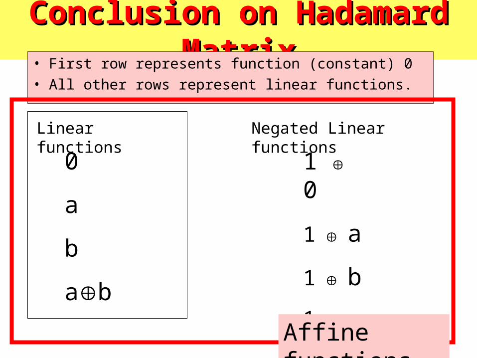
Conclusion on Hadamard MatrixConclusion on Hadamard Matrix• First row represents function (constant) 0

• All other rows represent linear functions.

Linear functions

0

a

b

ab

1 0

1 a

1 b

1 ab

Negated Linear functions

Affine functions

Quantum DJNow we additionally apply Hadamard in output of the function

This just comes from generalization of third method example

This slide shows that I can read function in phase encoding.

But this is of not much use itself.

Now formal proof

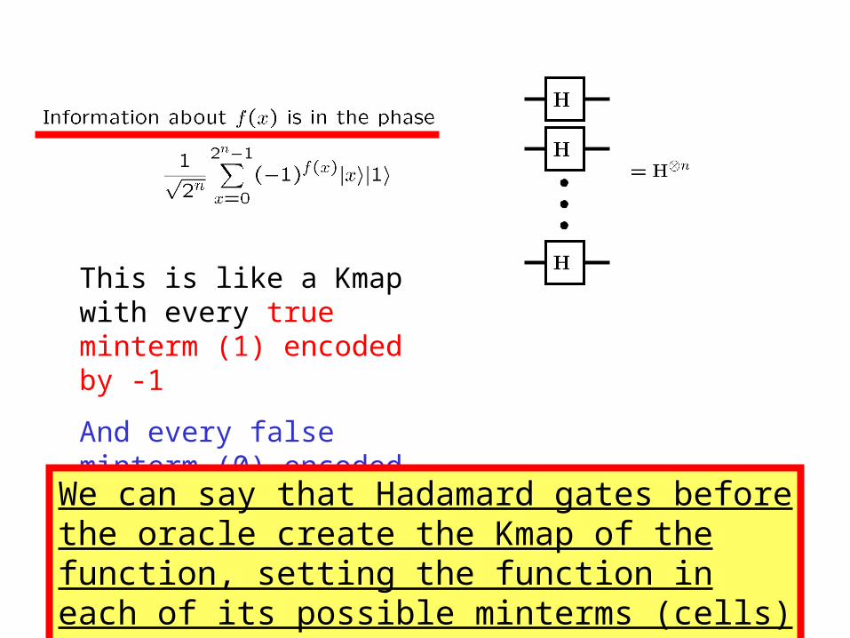
This is like a Kmap with every true minterm (1) encoded by -1

And every false minterm (0) encoded by 1

We can say that Hadamard gates before the oracle create the Kmap of the function, setting the function in each of its possible minterms (cells) in parallel

Motivating calculations for 3 variablesMotivating calculations for 3 variables• As we remember, these are transformations of Hadamard gate:

H|0> |0> + |1> H|1> |0> - |1>

H|x> |0> + (-1) x |1>

In general:

For 3 bits, vector of 3 Hadamards works as follows:

(|0>+(-1)a|1>) (|0>+(-1)b|1>) (|0>+(-1)c|1>) =From multiplication

|000> +(-1)c |001> +(-1)b |001>+(-1)b+c |001>000> +(-1)a |001> +

(-1)a+c |001> + (-1)a+b |001> (-1)a+b+c |001>

|abc>

We can formalize this as in the next slide:

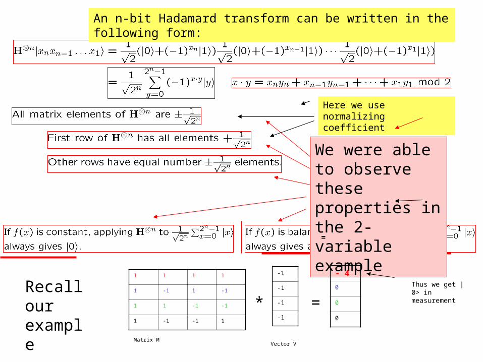
Here we use normalizing coefficient

An n-bit Hadamard transform can be written in the following form:

We were able to observe these properties in the 2-variable example

1 1 1 1

1 -1 1 -1

1 1 -1 -1

1 -1 -1 1

-1

-1

-1

-1

=

- 4

0

0

0

Matrix MVector V

* =Thus we get |0> in measurementRecall our

example

Full Quantum DJ - conclusion

Solves DJ with a SINGLE query vs 2n-1+1 classical deterministic!!!!!!!!!

If the reading is |00..0> then function is constant

If reading is other than |00..)> then the function is balanced

Deutsch-Josza Algorithm (contd)Deutsch-Josza Algorithm (contd)

• This algorithm distinguishes constant from balanced functions in one evaluationin one evaluation of f, versus 2n–1 + 1 evaluations for classical deterministic algorithms

• Balanced functions have many interesting and some useful properties– K. Chakrabarty and J.P. Hayes, “Balanced Boolean

functions,” IEE Proc: Digital Techniques, vol. 145, pp 52 - 62, Jan. 1998.

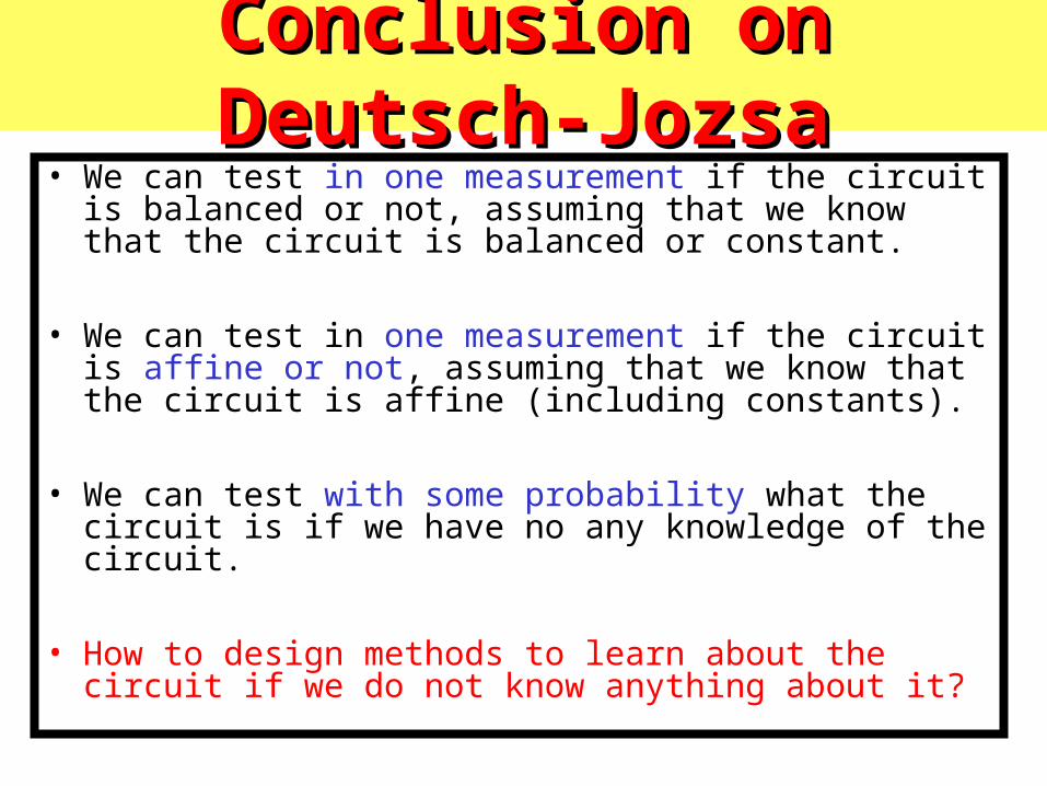
Conclusion on Deutsch-JozsaConclusion on Deutsch-Jozsa• We can test in one measurement if the circuit is balanced or not,

assuming that we know that the circuit is balanced or constant.

• We can test in one measurement if the circuit is affine or not, assuming that we know that the circuit is affine (including constants).

• We can test with some probability what the circuit is if we have no any knowledge of the circuit.

• How to design methods to learn about the circuit if we do not know anything about it?

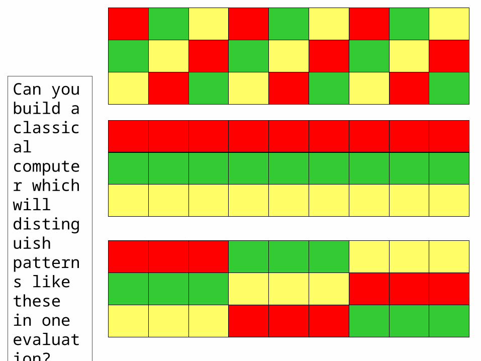
Can you build a classical computer which will distinguish patterns like these in one evaluation?

The answer is:The answer is:

• No, you cannot on a standard (classical) computer

• You can, using a ternary quantum computer

I leave this exercise to you, or it will be shown next lecture.

Local patterns for Affine Local patterns for Affine functionsfunctions

1 0 1 0

0 1 0 1

1 0 1 0

0 1 0 1

1 1 0 0

0 0 1 1

1 1 0 0

0 0 1 1

00 0111 10

00 01 11 10ab

cd

a b c d 1

Classically we need 5 tests (arbitrary cell and its all 4 Hamming distance-1 neighbors.

Quantumly we need just one test.

In red we show cells for which measurements should be done in classical computing to find the pattern.

Conclusion and questionsConclusion and questions

• We can test in one measurement if the circuit is balanced or not, assuming that we know that the circuit is balanced or constant.

• We can test in one measurement if the circuit is affine or not, assuming that we know that the circuit is affine (including constants).

• We can test with some probability what the circuit is if we have no any knowledge of the circuit.

• How to design methods to learn about the circuit if we do not know anything about it.

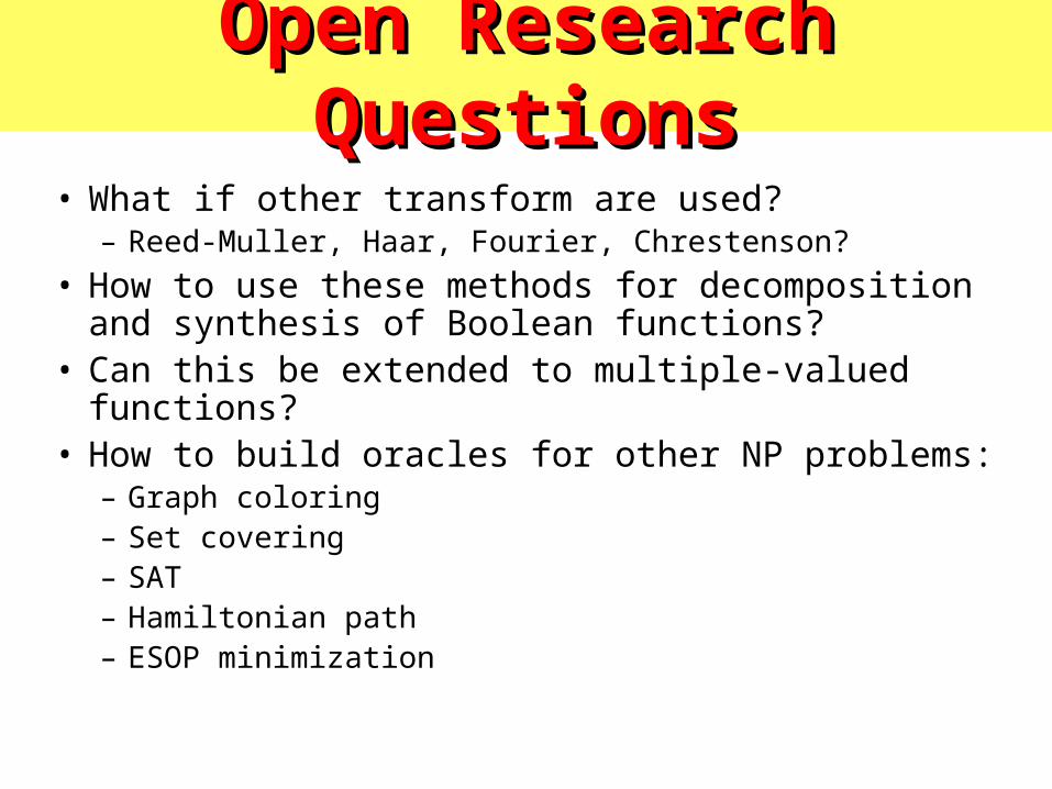
Open Research QuestionsOpen Research Questions

• What if other transform are used?– Reed-Muller, Haar, Fourier, Chrestenson?

• How to use these methods for decomposition and synthesis of Boolean functions?

• Can this be extended to multiple-valued functions?• How to build oracles for other NP problems:

– Graph coloring– Set covering– SAT– Hamiltonian path– ESOP minimization

Open Research QuestionsOpen Research Questions

• How to build Quantum Hough Transform?

• How to build efficient image processing algorithms?

• How to emulate them on standard FPGAs?

• How to emulate General Quantum Computers and Grover – like algorithms using FPGAs?

• How to use heuristic knowledge, such as a chromatic number to improve the speed of Grover Algorithm?

Open Research QuestionsOpen Research Questions

• How to test quantum circuits?

• How to design quantum circuits to make them even more highly testable?

• How to simulate quantum circuits more efficiently?

• How to invent quantum circuits for problems of Computational Intelligence?

• How to use quantum circuits to control robots?

The end