Revisiting displacement functions in three-dimensional elasticity of inhomogeneous media

International Journal of Solids and Structures 46 (2009) 3463–3470

Contents lists available at ScienceDirect

International Journal of Solids and Structures

journal homepage: www.elsevier .com/locate / i jsols t r

Revisiting displacement functions in three-dimensional elasticityof inhomogeneous media

M. Kashtalyan a,*, J.J. Rushchitsky b

a Centre for Micro- and Nanomechanics (CEMINACS), School of Engineering, University of Aberdeen, Fraser Noble Building, Aberdeen AB24 3UE, Scotland, UKb Timoshenko Institute of Mechanics, National Academy of Sciences of Ukraine, Nesterov Street 3, 03680 Kiev, Ukraine

a r t i c l e i n f o

Article history:Received 6 May 2008Received in revised form 29 April 2009Available online 6 June 2009

Keywords:ElasticityLinear elasticityThree-dimensional elasticity solutionAnalytical solutionsFunctionally graded materialsTransversely isotropic material

0020-7683/$ - see front matter � 2009 Elsevier Ltd. Adoi:10.1016/j.ijsolstr.2009.06.001

* Corresponding author.E-mail address: [email protected] (M. Kas

a b s t r a c t

The paper presents a three-dimensional solution to the equilibrium equations for linear elastic trans-versely isotropic inhomogeneous media. We assume that the material has constant Poisson’s ratios,and its Young’s and shear moduli have the same functional form of dependence on the co-ordinate nor-mal to the plane of isotropy. We show, apparently for the first time, that stresses and displacements insuch an inhomogeneous transversely isotropic elastic solid can be represented in terms of two displace-ment functions which satisfy the second- and fourth-order partial differential equations. We examineand discuss key aspects of the new representation; they include the relationship between the new dis-placement functions and Plevako’s solution for isotropic inhomogeneous material with constant Poisson’sratio as well as the application of the new representation to some important classes of three-dimensionalelasticity problems. As an example, the displacement function is derived that can be used to determinestresses and displacements in an inhomogeneous transversely isotropic half-space which is subjected to aconcentrated force normal to a free surface and applied at the origin (Boussinesq’s problem).

� 2009 Elsevier Ltd. All rights reserved.

1. Introduction

The three-dimensional linear elasticity problem of equilibriumof a deformable solid requires in general the solution of a set of15 coupled partial differential equations comprising three equa-tions of equilibrium, six stress–strain relations and six strain–displacement relations, with stress and/or displacementcomponents subject to appropriate boundary conditions. Usingthe displacement formulation, this set can be reduced to threecoupled second-order partial differential equations in terms ofdisplacements. For a homogeneous isotropic solid, the equilibriumequations in terms of displacements, also known as Navier’s equa-tions, can be further simplified by introducing potentials or dis-placement functions, the derivatives of which may be combinedto represent the displacement vector. These displacement func-tions are governed by equations such as the Laplace equation orbiharmonic equation, which have been thoroughly analysed bymathematicians. It is therefore often easier to find harmonic orbiharmonic displacement functions than to solve Navier’s equa-tions directly.

Displacement functions represent a powerful tool that helpssolve many important classes of problems, and for this reason theyhave been the subject of numerous studies in the literature. Forhomogeneous isotropic solids, classical solutions of Lamé,

ll rights reserved.

htalyan).

Papkovich–Neuber and Boussinesq–Galerkin are arguably the bestknown and most commonly used. However, other less known rep-resentations which give displacements and stresses in terms ofharmonic functions also exist, e.g. Youngdahl’s solution (1969).An overview of the displacement functions and the interrelationbetween many of the classical representations in three-dimen-sional linear elasticity is given, for example, in Chou and Pagano(1967).

For homogeneous transversely isotropic solids, displacementscan also be represented in terms of three quasi-harmonic displace-ment functions (Elliott, 1948), or two displacement functions thatsatisfy second- and fourth-order differential equations (Hu, 1953;Ding et al., 1996, 2006).

By comparison, displacement functions for inhomogeneouselastic solids have received much less attention in the literature.For an inhomogeneous isotropic solid with the shear modulus Gand the Poisson’s ratio m that depend on one spatial co-ordinateonly, Plevako (1971) derived solution to the three-dimensionalequilibrium equations in terms of displacements. He showed thatdisplacements can be represented in terms of two functions whichsatisfy the second- and the fourth-order partial differential equa-tions (see Appendix A). He also proved that in the case of a homo-geneous solid, these functions become harmonic and biharmonic,respectively, and that Papkovich’s solution is a particular case ofPlevako’s representation. In two-dimensional elasticity of the sameinhomogeneous solid, one of Plevako’s functions becomes zero,while the other is similar to the Airy stress function.

mailto:[email protected]

http://www.sciencedirect.com/science/journal/00207683

http://www.elsevier.com/locate/ijsolstr

3464 M. Kashtalyan, J.J. Rushchitsky / International Journal of Solids and Structures 46 (2009) 3463–3470

Plevako’s displacement functions have been recently used toderive a three-dimensional solution for a rectangular plate withexponential dependence of the shear modulus on the transverseco-ordinate (Kashtalyan, 2004). While showing the applicabilityof Plevako’s representation to the class of boundary-value prob-lems that allow separation of variables, it also provided a valuablebenchmark for validation of finite element models of functionallygraded plates (Zhen and Wanji, 2006); it was later used to investi-gate elastic deformation of coating/substrate systems of finitethickness (Kashtalyan and Menshykova, 2007, 2008a, 2009), andbending response of a sandwich panel with functionally gradedcore (Kashtalyan and Menshykova, 2008b).

It is our interest in the behaviour of these functionally gradedstructures and materials that was the motivation behind the pres-ent investigation.

In this paper, we revisit Plevako’s formulation and follow hissteps to derive solution to the equilibrium equations of thethree-dimensional elasticity for an inhomogeneous transverselyisotropic solid. While for homogeneous isotropic and transverselyisotropic solids many displacement functions exist, it is not thecase for inhomogeneous solids. To the best of our knowledge, dis-placement functions for inhomogeneous transversely isotropicmedia are introduced here for the first time.

We assume that the material has constant Poisson’s ratios andthe same functional form of dependence of the Young’s and shearmoduli on the co-ordinate normal to the plane of isotropy. Weshow, apparently for the first time, that stresses and displacementsin such an inhomogeneous transversely isotropic solid can be rep-resented in terms of two displacement functions which satisfy thesecond- and fourth-order partial differential equations. We exam-ine key aspects of the developed representation, including its rela-tion to Plevako’s representation for an inhomogeneous isotropicmaterial and application to some important classes of three-dimensional elasticity problems. Finally, an example is given thatdemonstrates use of the new displacement functions.

2. Problem formulation

2.1. Inhomogeneous transversely isotropic material

Let us consider an inhomogeneous transversely isotropic elasticmaterial referred to rectangular Cartesian co-ordinates x1; x2; x3, sothat any plane normal to the x3-axis is the plane of isotropy. Con-stitutive equations for such a material can be written asr11 ¼ c11e11 þ c12e22 þ c13e33 ð2:1aÞr22 ¼ c12e11 þ c11e22 þ c13e33 ð2:1bÞr33 ¼ c13e11 þ c13e22 þ c33e33 ð2:1cÞr23 ¼ 2c44e23 ð2:1dÞr13 ¼ 2c44e13 ð2:1eÞr12 ¼ 2c66e12 ¼ ðc11 � c12Þe12 ð2:1fÞwhere r and e are the stress and strain tensors, respectively, andc11; c12; c13; c33; c44 are five independent elastic constants. They canbe represented in terms of engineering constants E; E0; m; m0;G0 asfollows

c11 ¼1� ðm0Þ2ðE=E0Þ

1� m2 þ ð1þ 2mÞðm0Þ2ðE=E0ÞE ð2:2aÞ

c12 ¼v � ðm0Þ2ðE=E0Þ

1� m2 þ ð1þ 2mÞðm0Þ2ðE=E0ÞE ð2:2bÞ

c13 ¼m0ð1� mÞ

1� m2 þ ð1þ 2mÞðm0Þ2ðE=E0ÞE ð2:2cÞ

c33 ¼1� m2

1� m2 þ ð1þ 2mÞðm0Þ2ðE=E0ÞE0 ð2:2dÞ

c44 ¼ G0 ð2:2eÞ

where E; m and G ¼ E2ð1þmÞ are the Young’s modulus, the Poisson’s ra-

tio and the shear modulus in the plane of isotropy; E0; m0G0 are theYoung’s modulus, the Poisson’s ratio and the shear modulus inthe plane normal to the plane of isotropy.

Let us assume that:

(i) the Poisson’s ratio m; m0 are constant, i.e.

m ¼ const; m0 ¼ const ð2:3aÞ

(ii) the Young’s moduli E and E0, and the shear modulus G0, havethe same functional dependence on the co-ordinate x3, i.e.

Eðx3Þ ¼ Eomðx3Þ; Eo ¼ const ð2:3bÞE0ðx3Þ ¼ E0omðx3Þ; E0o ¼ const ð2:3cÞG0ðx3Þ ¼ G0omðx3Þ; G0o ¼ const ð2:3dÞwhere m ¼ mðx3Þ, henceforth termed the inhomogeneityfunction, is a sufficiently smooth function of the transverseco-ordinate x3. It follows from Eqs. (2.2) and (2.3) that theelastic constants c11; c12; c13; c33; c44 also have the same func-tional dependence on the transverse co-ordinate x3

c11ðx3Þ ¼ co11mðx3Þ ð2:4aÞ

c12ðx3Þ ¼ co12mðx3Þ ð2:4bÞ

c13ðx3Þ ¼ co13mðx3Þ ð2:4cÞ

c33ðx3Þ ¼ co33mðx3Þ ð2:4dÞ

c44ðx3Þ ¼ co44mðx3Þ ð2:4eÞ

where

co11 ¼

1� ðm0Þ2ðEo=E0oÞ1� m2 þ ð1þ 2mÞðm0Þ2ðEo=E0oÞ

Eo ð2:5aÞ

co12 ¼

v � ðm0Þ2ðEo=E0oÞ1� m2 þ ð1þ 2mÞðm0Þ2ðEo=E0oÞ

Eo ð2:5bÞ

co13 ¼

m0ð1� mÞ1� m2 þ ð1þ 2mÞðm0Þ2ðEo=E0oÞ

Eo ð2:5cÞ

co33 ¼

1� m021� m2 þ ð1þ 2mÞðm0Þ2ðEo=E0oÞ

E0o ð2:5dÞ

co44 ¼ G0o ð2:5eÞ

A particular case of stress–strain relations for an inhomoge-neous transversely isotropic material in the form of Eqs. (2.4), withan exponential inhomogeneity function mðx3Þ ¼ expðbx3Þ, was con-sidered by a number of researchers investigating functionallygraded piezoelectric (Zhong and Shang, 2003; Lu et al., 2006) andmagneto-electro-elastic (Pan and Han, 2005) plates.

2.2. Equilibrium equations in terms of displacements

In the absence of body forces, the equilibrium requires that

r11;1 þ r12;2 þ r13;3 ¼ 0 ð2:6aÞr12;1 þ r22;2 þ r23;3 ¼ 0 ð2:6bÞr13;1 þ r23;2 þ r33;3 ¼ 0 ð2:6cÞ

Here, comma denotes a derivative with respect to the spatial co-ordinates.

Strain–displacements relations are

eij ¼12ðui;j þ uj;iÞ ð2:7Þ

Upon substituting strain–displacement relations, Eq. (2.7), intothe constitutive relations, Eqs. (2.1), and then into the equilibriumequations, Eqs. (2.4), the equilibrium equations in terms of dis-placements are obtained. After some rearrangement, these can bewritten in the following form

M. Kashtalyan, J.J. Rushchitsky / International Journal of Solids and Structures 46 (2009) 3463–3470 3465

12ðc11 � c12Þu1;11 þ

12ðc11 � c12Þu1;22 þ c44u1;33 þ

12ðc11 þ c12Þu1;11

þ 12ðc11 þ c12Þu2;21 þ ðc44 þ c13Þu3;31

þ ðu1;3 þ u3;1Þc44;3 ¼ 0 ð2:8aÞ12ðc11 � c12Þu2;11 þ

12ðc11 � c12Þu2;22 þ c44u2;33 þ

12ðc11 þ c12Þu1;12

þ 12ðc11 þ c12Þu2;22 þ ðc44 þ c13Þu3;32

þ ðu2;3 þ u3;2Þc44;3 ¼ 0 ð2:8bÞ

c44u3;11 þ c44u3;22 þ12ðc11 � c12Þu3;33

þ c33 �c11 � c12

2

� �u3;33 þ ðc44 þ c13Þu1;13 þ ðc44 þ c13Þu2;23

þ c13;3u1;1 þ c13;3u2;2 þ c33;3u3;3 ¼ 0 ð2:8cÞ

Let us introduce the following new notations

e¼12ðc11þc12Þu1;1þ

12ðc11þc12Þu2;2þðc44þc13Þu3;3 ð2:9aÞ

e03¼ðc44þc13Þu1;13þðc44þc13Þu2;23þ c33�c11�c12

2

� �u3;33 ð2:9bÞ

D2¼@2

@x21

þ @2

@x22

ð2:9cÞ

g¼ 2c44

c11�c12¼ 2co

44

co11�co

12¼ go¼ const ð2:9dÞ

D3g ¼D2þgo @2

@x23

ð2:9eÞ

D3=g ¼D2þ1go

@2

@x23

ð2:9fÞ

Henceforth e will be termed the modified dilatation, and D3g

and D3=g the modified Laplacian operators. Constant go representsthe ratio between the shear moduli in the plane of isotropy andin the plane normal to it. For isotropic materials it is equal to unity,for transversely isotropic materials it can be used to characterisethe degree of anisotropy exhibited by the material.

In view of the notations, given by Eqs. (2.9), Eqs. (2.8) can be re-written as

ðc11 � c12ÞD3gu1 þ 2e;1 þ 2c44;3ðu1;3 þ u3;1Þ ¼ 0 ð2:10aÞðc11 � c12ÞD3gu2 þ 2e;2 þ 2c44;3ðu2;3 þ u3;2Þ ¼ 0 ð2:10bÞc44D3=gu3 þ e03 þ c13;3ðu1;1 þ u2;2Þ þ c33;3u3;3 ¼ 0 ð2:10cÞ

3. Analysis I

3.1. Displacement functions

Equilibrium equations in terms of displacements, Eqs. (2.10a,b),can be reduced to a single equation by differentiating Eq. (2.10a)with respect to x2, Eq. (2.10b) with respect to x1, and subtractingthe latter from the former. By doing so, the modified dilatation eis eliminated, so that

12ðc11 � c12ÞD2ðu1;2 � u2;1Þ þ

@

@x3c44

@

@x3ðu1;2 � u2;1Þ

� �¼ 0 ð3:1Þ

Let us introduce two displacement functions U ¼ Uðx1; x2; x3Þand F ¼ Fðx1; x2; x3Þ, so that

u1 ¼@U@x2þ @F@x1

; u2 ¼ �@U@x1þ @F@x2

; u3 ¼ u3 ð3:2Þ

By substituting Eq. (3.2) into Eq. (3.1) and into Eqs. (2.10a–c), itcan be established that function U must satisfy the following par-tial differential equation

12ðc11 � c12ÞD2Uþ

@

@x3c44

@U@x3

� �¼ 0 ð3:3aÞ

Due to the same functional form of dependence of elastic con-stants on the x3 co-ordinate, Eqs. (2.4), and the notation, given byEq. (2.9c), the above equation can be re-written as

mðx3ÞD2Uþ go @

@x3mðx3Þ

@U@x3

� �¼ 0 ð3:3bÞ

Function F and displacement u3 can be found from the followingequations12ðc11 � c12ÞD3gF þ 1

2ðc11 þ c12ÞD2F þ c44;3

@F@x3þ u3

� �þ ðc44 þ c13Þu3;3 ¼ 0 ð3:4aÞ

c44D3=gu3 þ c33 �c11 � c12

2

� �u3;33 þ c33;3u3;3

þ D2 ðc44 þ c13Þ@F@x3þ c13;3F

� �¼ 0 ð3:4bÞ

These equations can be re-written as

c11D2F þ c13u3;3 þ@

@x3c44

@F@x3þ u3

� �� ¼ 0 ð3:5aÞ

c44D2@F@x3þ u3

� �þ @

@x3½c33u3;3 þ c13D2F� ¼ 0 ð3:5bÞ

Let us introduce a new function, W, so that Eq. (3.5b) becomesan identity

c44@F@x3þ u3

� �¼ �D2

@W@x3

ð3:6aÞ

c33u3;3 þ c13D2F ¼ D2D2W ð3:6bÞ

Using Eq. (3.6a), (3.5a) can be re-written as

c11D2F þ c13u3;3 �@2

@x23

D2W ¼ 0 ð3:7Þ

By eliminating u3;3 from Eqs. (3.6b) and (3.7), a relationship be-tween functions F and and W is established as

F ¼ � 1c11c33 � c2

13

c13D2 � c33@2

@x23

" #W ð3:8aÞ

or alternatively

F ¼ � 1c11c33 � c2

13

c13DW� ðc13 þ c33Þ@2W@x2

3

" #ð3:8bÞ

where D is the Laplacian operator.

3.2. Representation of displacements and stresses

On referring to Eqs. (3.2) and (3.8), the two components of thedisplacement vector can be represented in terms of displacementfunctions U and W as

u1 ¼@U@x2� 1

c11c33 � c213

c13D2 � c33@2

@x23

" #@W@x1

ð3:9aÞ

u2 ¼ �@U@x1� 1

c11c33 � c213

c13D2 � c33@2

@x23

" #@W@x2

ð3:9bÞ

The third displacement component is found from Eqs. (3.6a)and (3.8) as

u3 ¼ �1

c44D2

@W@x3

þ @

@x3

c13

c11c33 � c213

D2 �c33

c11c33 � c213

@2

@x23

" #W ð3:9cÞ


Due to the same functional form of dependence of elastic con-stants on the x3 co-ordinate, Eqs. (2.4), the above representationbecomes

u1 ¼@U@x2� m�1ðx3Þ

co11co

33 � co2

13

co13D2 � co

33@2

@x23

" #@W@x1

ð3:10aÞ

u2 ¼ �@U@x1� m�1ðx3Þ

co11co

33 � co2

13

co13D2 � co

33@2

@x23

" #@W@x2

ð3:10bÞ

u3 ¼ �m�1ðx3Þ

co44

D2@W@x3

þ @

@x3

co13m�1ðx3Þ

co11co

33 � co2

13

D2 �co

33m�1ðx3Þco

11co33 � co2

13

@2

@x23

" #W ð3:10cÞ

The representation, given by Eqs. (3.9), can also be written usingthe Laplacian operator D as

u1 ¼@U@x2� 1

c11c33 � c213

c13D� ðc13 þ c33Þ@2

@x23

" #@W@x1

ð3:11aÞ

u2 ¼ �@U@x1� 1

c11c33 � c213

c13D� ðc13 þ c33Þ@2

@x23

" #@W@x2

ð3:11bÞ

u3 ¼ �1

c44D� @2

@x23

!@W@x3

þ @

@x3

c13

c11c33 � c213

DW� c13 þ c33

c11c33 � c213

@2W@x2

3

" #ð3:11cÞ

Since the functional form of dependence of elastic constants onthe x3 co-ordinate is the same, Eqs. (2.4), the representation, givenby Eqs. (3.10), can be written as

u1 ¼@U@x2� m�1ðx3Þ

co11co

33 � co2

13

co13D� ðco

13 þ co33Þ

@2

@x23

" #@W@x1

ð3:12aÞ

u2 ¼ �@U@x1� m�1ðx3Þ

co11co

33 � co2

13

co13D� ðco

13 þ co33Þ

@2

@x23

" #@W@x2

ð3:12bÞ

u3 ¼ �m�1ðx3Þ

co44

D� @2

@x23

!@W@x3

þ @

@x3

co13m�1ðx3Þ

co11co

33 � co2

13

DW� ðco13 þ co

33Þm�1ðx3Þco

11co33 � co2

13

@2W@x2

3

" #ð3:12cÞ

Representation of displacement in terms of two functions, Uand W, given by Eqs. (3.9)–(3.12), is valid for any kind of inhomo-geneous transversely isotropic material provided it satisfies theassumptions, given by Eqs. (2.3).

The components of the stress tensor can be expressed in termson functions U and W using representations, Eqs. (3.9a–c), strain–displacement relations, Eq. (2.7), and constitutive equations fortransversely isotropic material, Eqs. (2.1).

3.3. Equation for function W

First, a derivative u3;3 is calculated by differentiating Eq. (3.6a)over x3 as

u3;3 ¼ �@2F@x2

3

� @

@x3

1c44

D2@W@x3

� �ð3:13Þ

Substitution of the above derivative into Eq. (3.6b), leads to

�c33@

@x3

1c44

D2@W@x3

� �þ c13D2 � c33

@2

@x23

" #F ¼ D2D2W ð3:14Þ

Taking into account that function F is given by Eq. (3.8), theabove equation is transformed into

D2D2Wþ c33@

@x3

1c44

D2@W@x3

� �� c33

@2

@x23

� c13D2

" #

� c13

c11c33 � c213

D2 �c33

c11c33 � c213

@2

@x23

" #W ¼ 0 ð3:15Þ

After some rearrangement, it can be re-written as

c11D2D2W�c13D2@2W@x2

3

þðc11c33�c213Þ�

@

@x3

1c44

D2@W@x3

� ��

þ @2

@x23

c33

c11c33�c213

@2W@x2

3

" #� @2

@x23

c13

c11c33�c213

D2W� �)

¼0 ð3:16aÞ

Due to the same functional form of dependence of elastic con-stants on the x3 co-ordinate, Eqs. (2.4), the above equation becomes

co11D2D2W� co

13D2@2W@x2

3

þ co11co

33 � co2

13

� �mðx3Þ

� 1co

44

@

@x3m�1ðx3ÞD2

@W@x3

� �þ co

33

co11co

33 � co2

13

@2

@x23

m�1ðx3Þ@2W@x2

3

" #(

� co13

co11co

33 � co2

13

@2

@x23

m�1ðx3ÞD2W )

¼ 0 ð3:16bÞ

Now, partial differential equations for functions U, Eqs. (3.3),and W, Eqs. (3.16) are uncoupled.

4. Analysis II

In this section, we analyse and discuss some key aspects of thedeveloped representation. Rather than adding specific examplesdemonstrating the application of the new displacement functions,we examine the usefulness of the new representation in broad terms,i.e. by showing its applicability to whole classes of three-dimen-sional elasticity problems, such as the class of boundary-value prob-lems that allow separation of variables. Within this class we examinetwo important inhomogeneity functions – the exponential functionand the power law – and show how the equations simplify in eachcase. For instance, we show that for the exponential inhomogeneityfunction the equations for two new displacement functions reduceto Helmholtz’s equations and the second- and fourth-order ordinarydifferential equations with constant coefficients, particular solu-tions to which can be found following a standard routine.

We also show that on transition to the isotropic material thenew representation for transversely isotropic inhomogeneousmaterial coincides with Plevako’s representation for isotropic inho-mogeneous material.

4.1. Transition to isotropic material

Constitutive equations for isotropic material are given by Eqs.(2.1) with

c11 ¼ c33 ¼Eð1� mÞ

ð1þ mÞð1� 2mÞ ; c12 ¼ c13 ¼Em

ð1þ mÞð1� 2mÞ ;

c44 ¼ G; G ¼ E2ð1þ mÞ ð4:1aÞ

It follows from Eq. (4.1a) that

c13

c11c33 � c213

¼ m2G

;c13 þ c33

c11c33 � c213

¼ 12G

ð4:1bÞ

Then the representation of displacements in terms of two dis-placement functions U and W, given by Eqs. (3.11), fully coincideswith that obtained by Plevako (1971) – see Appendix A, Eq. (A.2) –with functions U and W corresponding to Plevako’s N and L,respectively.


4.2. Separation of variables

Suppose the boundary conditions and the applied loadings aresuch that the three-dimensional elasticity problem allows separa-tion of variables in the displacement functions in the form

Uðx1; x2; x3Þ ¼ U__

ðx1; x2ÞU_

ðx3Þ ð4:2aÞ

Wðx1; x2; x3Þ ¼ W__

ðx1; x2ÞW_

ðx3Þ ð4:2bÞ

Substitution of these representations into equations for func-tions U and W, Eqs. (3.3b) and (3.16b), yields the following four dif-ferential equations:

D2 U__

þk2U U__

¼ 0 ð4:3aÞ

D2 W__

þk2W W

__

¼ 0 ðor D2 W__

�k2W W

__

¼ 0Þ ð4:3bÞ

d2

dx23

þm0ðx3Þmðx3Þ

ddx3� k2

U

go

" #U_

¼ 0 ð4:4aÞ

mðx3Þd2

dx23

m�1ðx3Þd2 W

_

dx23

24

35� k2

Wmðx3Þd2

dx23

m�1ðx3ÞW_h i

þ co11co

33 � co2

13

co33co

44k2

Wmðx3Þd

dx3m�1ðx3Þ

d W_

dx3

24

35

� co13

co33

k2W

d2 W_

dx23

þ co11

co33

k4W W

_

¼ 0 ð4:4bÞ

Eqs. (4.3a and b) are the Helmholtz’s equations, which have partic-ular solutions in the form

f ðx1; x2Þ ¼ exp½iðkf 1x1 þ kf 2x2Þ�; k2f 1 þ k2

f 1 ¼ k2f ð4:5aÞ

f ðx1; x2Þ ¼ ðAþ Bx1Þ exp½iðkf x1Þ� þ ðC þ Dx2Þ exp½iðkf x2Þ�;

f � U__

;W__

ð4:5bÞ

Eqs. (4.4a and b), are second- and fourth-order ordinary lineardifferential equations with variable coefficients, which depend onthe inhomogeneity function m ¼ mðx3Þ that characterises thedependence of the Young’s and shear moduli of the inhomoge-neous transversely isotropic material on the co-ordinate x3. Theycan be simplified further once the inhomogeneity functionm ¼ mðx3Þ is specified.

4.3. Inhomogeneity functions

When the inhomogeneity function is an exponential one, i.e.mðx3Þ ¼ exp ax3, equations Eqs. (4.4a and b) reduce to second-and fourth-order differential equations with constantcoefficients

d2

dx23

þ ad

dx3� k2

U

go

" #U_

¼ 0 ð4:6aÞ

d4 W_

dx43

� 2ad3 W

_

dx33

þ a2 � 2co

13

co33

k2W

co11co

33 � co2

13

co33co

44k2

W

" #d2 W

_

dx23

þ ak2W 2

co13

co33� co

11co33 � co2

13

co33co

44

" #d W_

dx3

þ k2W

co33

co11k2

W � co13a

2� �

W_

¼ 0 ð4:6bÞ

Particular solutions to Eqs. (4.6a and b) can be found following astandard routine.

For a power-law dependence of the elastic constants on theco-ordinate x3 in the form mðx3Þ ¼ xb

3, Eq. (4.4a) reduces toequation

d2

dx23

þ bx3

ddx3� k2

U

go

" #U_

¼ 0 ð4:7aÞ

Eq. (4.7a) is a transformed Bessel equation, solution to which isgiven by

U_

ðx3Þ ¼ C1xnJn i

ffiffiffiffiffiffik2

U

go

sx3

0@

1Aþ C1xnYn i

ffiffiffiffiffiffik2

U

go

sx3

0@

1A ð4:7bÞ

where

n ¼ 1� b2

; c ¼ k2U

goð4:7cÞ

Fourth-order ordinary differential equation for function /__

, Eq.(4.4b), reduces to

d4 W_

dx43

� 2bx3

d3 W_

dx33

þ bðbþ 1Þx2

3

� 2co

13

co33

k2W þ

co11co

33 � co2

13

co33co

44k2

W

" #d2 W

_

dx23

þ bx3

2co

13

co33

k2W �

co11co

33 � co2

13

co33co

44k2

W

" #d W_

dx3

þ co11

co33

k4W �

co13

co33

k2W

bðbþ 1Þx2

3

� �W_

¼ 0 ð4:8Þ

Solution of this equation is not as straightforward as that of Eqs.(4.7) and must be sought using more general methods, such as apower-series method.

5. Example

In this section, an example is considered in order to demon-strate how the new displacement functions can be used to deter-mine stresses and displacements in an inhomogeneoustransversely isotropic half-space x3 P 0 which is subjected to aconcentrated force normal to a free surface and applied at theorigin. For a homogeneous isotropic half-space, such problemwas first considered by Boussinesq (1885) and bears his name.As pointed out by Selvadurai (2001), the solution to Boussinesq’sproblem can be obtained by several methods. The first approachconsists of reducing the problem to a boundary-value problem inpotential theory. For isotropic homogeneous half-space, whenthe surface of the half-space is subjected to normal tractionsonly, the elasticity problem is reduced to that of finding a singleharmonic function. The solution to the concentrated force prob-lem is recovered as a special case of the general normal loading.The second approach to the solution of Boussinesq’s problemcommences with Kelvin’s solution for the point force acting atthe interior of an infinite space. It utilizes a distribution of com-binations of dipoles, which are equivalent to a distribution ofcentres of compression along an axis, to eliminate the shear trac-tions occurring on the plane normal to the line of action of theKelvin force, thereby recovering Boussinesq’s solution. A thirdapproach involves the application of integral transform tech-niques to the solution of a governing partial differential equationwhich can be then used to explicitly satisfy the traction bound-ary condition.

Taking into account the axial symmetry of the Boussinesq’sproblem, let us introduce a cylindrical co-ordinate systemðr; h; zÞ such that z-axis coincides with x3-axis, and adopt theexponential variation of the elastic constants with the transverseco-ordinate z ðz P 0Þ in the form


mðzÞ ¼ expðczÞ; c 6 0 ð5:1Þ

Due to the axial symmetry, one of the displacement functions isU ¼ 0, while the differential equation for the other displacementfunction W, Eq. (3.16b), in cylindrical co-ordinates becomes

@4W@z4 � 2c

@3W@z3 þ ðBD2 þ c2Þ @

2W@z2 þþBcD2

@W@z

þ � co13

co33

c2 þ co11

co33

D2

� �D2W ¼ 0 ð5:2aÞ

where

B ¼ co11co

33 � co2

13 � 2co13co

44

co33co

44ð5:2bÞ

D2 �d2

dr2 þ1r

ddr

ð5:2cÞ

Function W is sought in the form

Wðr; zÞ ¼Z 1

0AðnÞJ0ðnrÞwðz; nÞdn ð5:3aÞ

where AðnÞ is an arbitrary function, J0ðnrÞ is Bessel function of thefirst kind of order n ¼ 0, which satisfies Bessel’s equation

d2J0

dr2 þ1r

dJ0

drþ n2J0 ¼ 0; n > 0 ð5:3bÞ

and wðz; nÞ is an unknown function. Substitution of Eqs. (5.3) intoEq. (5.2a) leads to the following equation for the function wðz; nÞ

d4w

dz4 �2cd3w

dz3 þðc2�Bn2Þd

2w

dz2 ��Bcn2 dwdz� co

13

co33

c2þco11

co33

n2� �

n2w¼0

ð5:4Þ

To simplify Eq. (5.4), let us introduce new variables

~c ¼ nc; f ¼ nz ð5:5Þ

Then Eq. (5.4) reduces to

d4w

df4 � 2~cd3w

df3 þ ð~c2 � BÞd

2w

df2 � B~cdwdf� co

13

co33

~c2 þ co11

co33

� �w ¼ 0 ð5:6Þ

Eq. (5.4) is the fourth-order ordinary differential equation withconstant coefficients, which can be solved following a standardroutine. On substitution of a trial solution w ¼ expðsfÞ, the charac-teristic equation, corresponding to Eq. (5.6), is obtained as

s4 � 2~cs3 þ ð~c2 � BÞs2 � B~cs� co13

co33

~c2 þ co11

co33

� �¼ 0 ð5:7Þ

Following the Descartes–Euler method (Korn and Korn, 2000),the above equation can be transformed to the reduced form

t4 þ Pt2 þ Qt þ R ¼ 0 ð5:8aÞ

through the substitution

s ¼ t þ ~c=2 ð5:8bÞ

where

P ¼ �~c2

2þ B; Q ¼ �2~cB; R ¼

~c4

16� 3B

~c2

4� co

13

co33

~c2 þ co11

co33

� �ð5:8cÞ

Then, the roots of the characteristic equation, Eq. (5.7), are givenas

s1;2;3;4 ¼~c2� ffiffiffiffiffi

y1p � ffiffiffiffiffi

y2p � ffiffiffiffiffi

y3p ð5:9aÞ

with the signs of the square roots chosen so that

ffiffiffiffiffiy1p ffiffiffiffiffi

y2p ffiffiffiffiffi

y3p ¼

~cB4¼

~c4� c

o11co

33 � co2

13 � 2co13co

44

co33co

44ð5:9bÞ

Here y1; y2; y3 are the roots of the following cubic equation, whichcorresponds to Eq. (5.8a),

y3 þ ay2 þ byþ c ¼ 0 ð5:10aÞ

a ¼ P2; b ¼ P2 � 4R

16; c ¼ �Q 2

64ð5:10bÞ

They given by the Cardan’s solution (Korn and Korn, 2000) as

y1;2;3 ¼ �a3þ Y1;2;3 ð5:11aÞ

where

Y1 ¼ffiffiffiffiffiffiffiffiffiffiffiffiffiffiffiffiffiffiffiffiffiffi�M

2þ

ffiffiffiffiKp3

rþ

ffiffiffiffiffiffiffiffiffiffiffiffiffiffiffiffiffiffiffiffiffiffi�M

2�

ffiffiffiffiKp3

rð5:11bÞ

Y2;3 ¼ �12


2þ

ffiffiffiffiKp3

rþ


2�

ffiffiffiffiKp3

r !

� i

ffiffiffi3p

2


2þ

ffiffiffiffiKp3

r�


2�

ffiffiffiffiKp3

r !ð5:11cÞ

M ¼ 2a3

� �3� ab

3þ c; K ¼ 1

3� a2

3þ b

� �� 3

þ M2

� �2

ð5:11dÞ

The above cubic equation has either one real root and two con-jugate complex roots, or three real roots of which at least two areequal, or three different real roots, if K is positive, zero or negative,respectively (Korn and Korn, 2000).

Finally, the displacement function W for the Boussinesq’s prob-lem for an inhomogeneous transversely isotropic half-space hasthe form

Wðr; zÞ ¼Z 1

0AðnÞJ0ðnrÞfC1 exp½s1ðnÞnz� þ C2 exp½s2ðnÞnz�

þ C3 exp½s3ðnÞnz� þ C4 exp½s4ðnÞnz�gdn ð5:12Þ

where constants C1;C2;C3;C4 must be chosen so as to match givenboundary conditions. The integral in the above equation, Eq. (5.12),involving exponential functions and Bessel functions of the firstkind of order n ¼ 0, cannot be presented in closed form and hasto be integrated numerically using, for example, an approach devel-oped by Wang et al. (2003). Full analysis of the Boussinesq’s prob-lem will be reported in a separate publication.

6. Conclusions

A set of 15 governing equations of the three-dimensional linearelasticity may be reduced to three coupled partial differentialequations in terms of displacements and then further simplifiedby introducing appropriately chosen displacement functions.While for homogenous isotropic and transversely isotropic solidsmany displacement functions exist, it is not the case for inhomoge-neous solids.

In this paper, we have revisited Plevako’s displacement func-tions for inhomogeneous isotropic solids for the purpose of deriv-ing a solution to the equilibrium equations of three-dimensionallinear elasticity for inhomogeneous transversely isotropic solids.To the best of our knowledge, displacement functions for inhomo-geneous transversely isotropic media have been introduced herefor the first time.

With the help of two displacement functions it proved possibleto uncouple the equilibrium equations in terms of displacementsand to reduce the number of partial differential equations requir-ing solution from three to two.

The uncoupled partial differential equations for two displace-ment functions allow separation of variables, which opens newpossibilities for further simplification. It is established that the dis-placement functions are governed by Helmholtz’s equations in the


plane of isotropy, and ordinary differential equations of the sec-ond- and fourth-order with variable coefficients with respect tothe co-ordinate normal to the plane of isotropy.

When the inhomogeneity function is an exponential one, thelatter reduce to the second- and fourth-order ordinary differentialequations with constant coefficients, which can be solved usingstandard routines. For the power-law inhomogeneity function,the second-order differential equation reduces to the modified Bes-sel equation, while the fourth-order one still represents achallenge.

On transition to the isotropic material, the new representationfor transversely isotropic inhomogeneous material coincides withPlevako’s representation for isotropic inhomogeneous material.As mentioned in the Introduction, Plevako’s displacement func-tions were successfully used to investigate three-dimensional elas-tic deformations of structures incorporating functionally gradedmaterials, including coating/substrate systems and sandwichconstructions.

As an example, the displacement function is derived that can beused to determine stresses and displacements in an inhomoge-neous transversely isotropic half-space which is subjected to a con-centrated force normal to a free surface and applied at the origin(Boussinesq’s problem).

It is hoped that this paper will be viewed as making a contribu-tion towards the fundamentals of the three-dimensional elasticitytheory. By focussing solely on the rigorous mathematical develop-ment of the new displacement functions and discussion of theirusefulness in broad terms, the paper communicates new knowl-edge of fundamental nature which can be used by other research-ers to solve further issues according to their specific researchinterests (just as we used Plevako’s functions according to our re-search interests).

Acknowledgements

Financial support of this research by the University of AberdeenVisiting Scholars’, the Royal Society of Edinburgh International Ex-change Programme and the Royal Society International Joint Pro-ject grants is gratefully acknowledged.

Appendix A

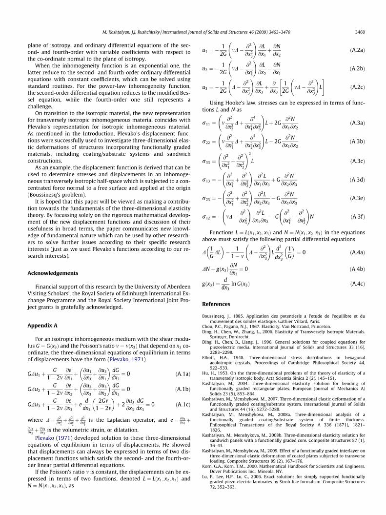
For an isotropic inhomogeneous medium with the shear modu-lus G ¼ Gðx3Þ and the Poisson’s ratio m ¼ mðx3Þ that depend on x3 co-ordinate, the three-dimensional equations of equilibrium in termsof displacements have the form (Plevako, 1971)

GDu1 þG

1� 2m@e@x1þ @u1

@x3þ @u3

@x1

� �dGdx3¼ 0 ðA:1aÞ

GDu2 þG

1� 2m@e@x2þ @u2

@x3þ @u3

@x2

� �dGdx3¼ 0 ðA:1bÞ

GDu3 þG

1� 2m@e@x3þ e

ddx3

2Gm1� 2m

� �þ 2

@u3

@x3

dGdx3¼ 0 ðA:1cÞ

where D ¼ @2

@x21þ @2

@x22þ @2

@x23

is the Laplacian operator, and e ¼ @u1@x1þ

@u2@x2þ @u3

@x3is the volumetric strain, or dilatation.

Plevako (1971) developed solution to these three-dimensionalequations of equilibrium in terms of displacements. He showedthat displacements can always be expressed in terms of two dis-placement functions which satisfy the second- and the fourth-or-der linear partial differential equations.

If the Poisson’s ratio m is constant, the displacements can be ex-pressed in terms of two functions, denoted L ¼ Lðx1; x2; x3Þ andN ¼ Nðx1; x2; x3Þ, as

u1 ¼ �1

2GmD� @2

@x23

!@L@x1þ @N@x2

ðA:2aÞ

u2 ¼ �1

2GmD� @2

@x23

!@L@x2� @N@x1

ðA:2bÞ

u3 ¼ �1

2GD� @2

@x23

!@L@x3þ @

@x3

12G

mD� @2

@x23

!L

" #ðA:2cÞ

Using Hooke’s law, stresses can be expressed in terms of func-tions L and N as

r11 ¼ m@2

@x22

Dþ @4

@x21@x2

3

!Lþ 2G

@2N@x1@x2

ðA:3aÞ

r22 ¼ m@2

@x21

Dþ @4

@x22@x2

3

!L� 2G

@2N@x1@x2

ðA:3bÞ

r33 ¼@2

@x21

þ @2

@x22

!2

L ðA:3cÞ

r13 ¼ �@2

@x21

þ @2

@x22

!@2L

@x1@x3þ G

@2N@x2@x3

ðA:3dÞ

r23 ¼ �@2

@x21

þ @2

@x22

!@2L

@x2@x3� G

@2N@x1@x3

ðA:3eÞ

r12 ¼ � mD� @2

@x23

!@2L

@x1@x2� G

@2

@x21

� @2

@x22

!N ðA:3fÞ

Functions L ¼ Lðx1; x2; x3Þ and N ¼ Nðx1; x2; x3Þ in the equationsabove must satisfy the following partial differential equations

D1G

DL� �

� 11� m

D� @2

@x23

!L

d2

dx23

1G

� �¼ 0 ðA:4aÞ

DN þ gðx3Þ@N@x3¼ 0 ðA:4bÞ

gðx3Þ ¼d

dx3ln Gðx3Þ ðA:4cÞ

References

Boussinesq, J., 1885. Application des potentiesls a l’etude de l’equilibre et dumouvement des solides elastique. Gathier Villard, Paris.

Chou, P.C., Pagano, N.J., 1967. Elasticity. Van Nostrand, Princeton.Ding, H., Chen, W., Zhang, L., 2006. Elasticity of Transversely Isotropic Materials.

Springer, Dordrecht.Ding, H., Chen, B., Liang, J., 1996. General solutions for coupled equations for

piezoelectric media. International Journal of Solids and Structures 33 (16),2283–2298.

Elliott, H.A., 1948. Three-dimensional stress distributions in hexagonalaeolotropic crystals. Proceedings of Cambridge Philosophical Society 44,522–533.

Hu, H., 1953. On the three-dimensional problems of the theory of elasticity of atransversely isotropic body. Acta Scientia Sinica 2 (2), 145–151.

Kashtalyan, M., 2004. Three-dimensional elasticity solution for bending offunctionally graded rectangular plates. European Journal of Mechanics A/Solids 23 (5), 853–864.

Kashtalyan, M., Menshykova, M., 2007. Three-dimensional elastic deformation of afunctionally graded coating/substrate system. International Journal of Solidsand Structures 44 (16), 5272–5288.

Kashtalyan, M., Menshykova, M., 2008a. Three-dimensional analysis of afunctionally graded coating/substrate system of finite thickness.Philosophical Transactions of the Royal Society A 336 (1871), 1821–1826.

Kashtalyan, M., Menshykova, M., 2008b. Three-dimensional elasticity solution forsandwich panels with a functionally graded core. Composite Structures 87 (1),36–43.

Kashtalyan, M., Menshykova, M., 2009. Effect of a functionally graded interlayer onthree-dimensional elastic deformation of coated plates subjected to transverseloading. Composite Structures 89 (2), 167–176.

Korn, G.A., Korn, T.M., 2000. Mathematical Handbook for Scientists and Engineers.Dover Publications Inc., Mineola, NY.

Lu, P., Lee, H.P., Lu, C., 2006. Exact solutions for simply supported functionallygraded piezo-electric laminates by Stroh-like formalism. Composite Structures72, 352–363.


Pan, E., Han, F., 2005. Exact solution for functionally graded and layered magneto-electro-elastic plates. International Journal of Engineering Science 43 (3–4),321–339.

Plevako, V.P., 1971. On the theory of elasticity of inhomogeneous media. Journal ofApplied Mathematics and Mechanics 35 (5), 806–813.

Selvadurai, A.P.S., 2001. On Boussinesq’s problem. International Journal ofEngineering Science 39 (1), 317–322.

Wang, C.D., Tzeng, C.S., Pan, E., Liao, J.J., 2003. Displacement and stresses due to avertical point load in an inhomogeneous transversely isotropic half-space.International Journal of Rock Mechanics and Mining Sciences 40 (4), 667–685.

Youngdahl, C.K., 1969. On the completeness of a set of stress functions appropriateto the solution of elasticity problems in general cylindrical coordinates.International Journal of Engineering Science 7 (1), 61–79.

Zhen, W., Wanji, C., 2006. A higher-order theory and refined three-node triangularelement for functionally graded plates. European Journal of Mechanics A/Solids25, 447–463.

Zhong, Z., Shang, E.T., 2003. Three-dimensional exact analysis of a simply supportedfunctionally gradient piezoelectric plate. International Journal of Solids andStructures 40 (20), 853–864.

Documents

Revisiting displacement functions in three-dimensional elasticity of inhomogeneous media