1

Introduction and the Hodgkin-Huxley Model

Richard Bertram

Department of Mathematics and

Programs in Neuroscience and Molecular Biophysics

Florida State University

Tallahassee, Florida 32306

2

Reference: Chapters 2 and 3 of the Sterratt/Graham/Gillies/Willshaw

text.

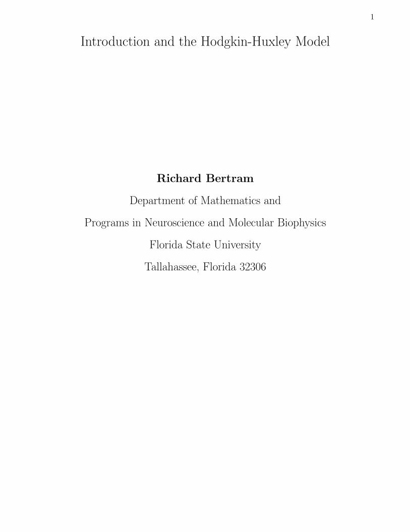
The neuron is the basic unit of the nervous system. It is a normal cell

that has been adapted morphologically and in terms of protein expression

for direct communication with other neurons, with various receptors (e.g.,

photoreceptors), and with muscle tissue.

Figure 1: Stained single neuron

Dendrites: input pathways, from afferent neurons

3

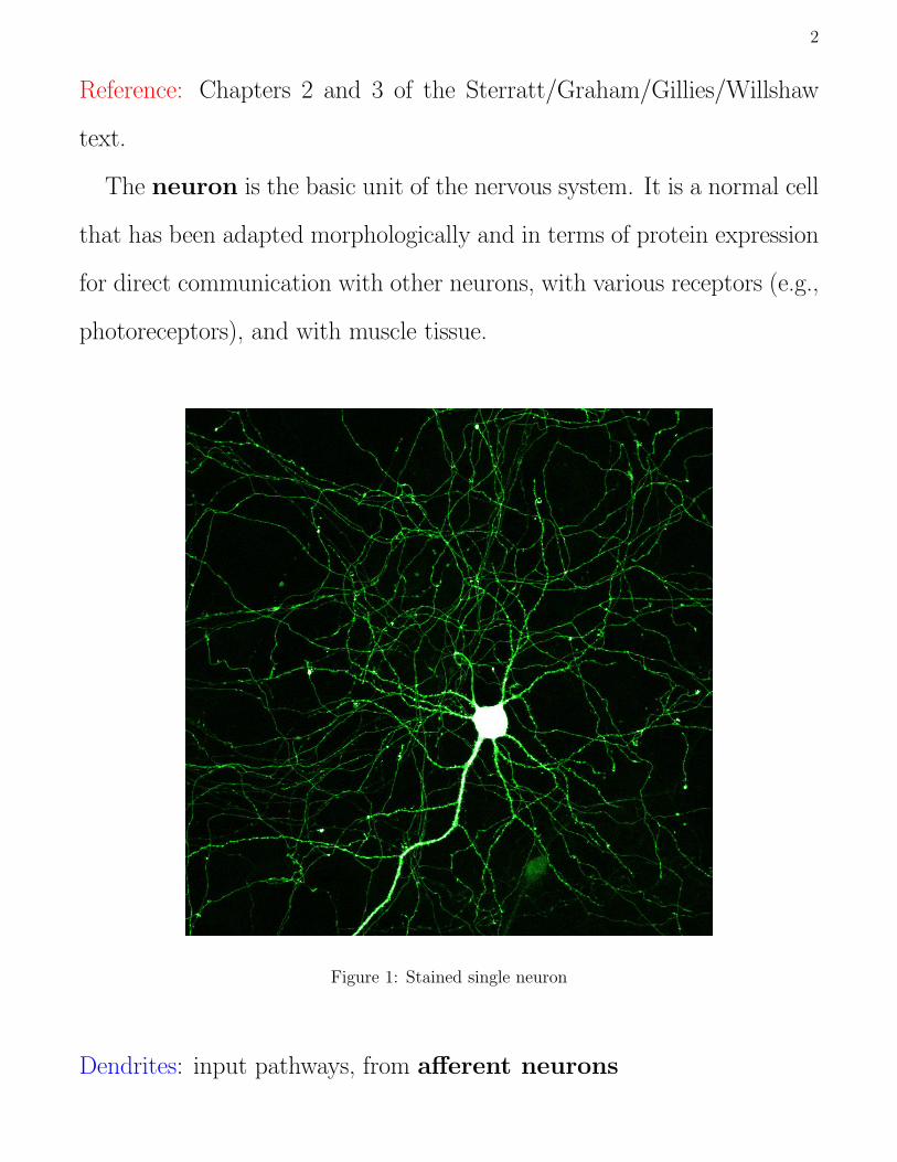
Figure 2: Population of interconnected stained neurons

4

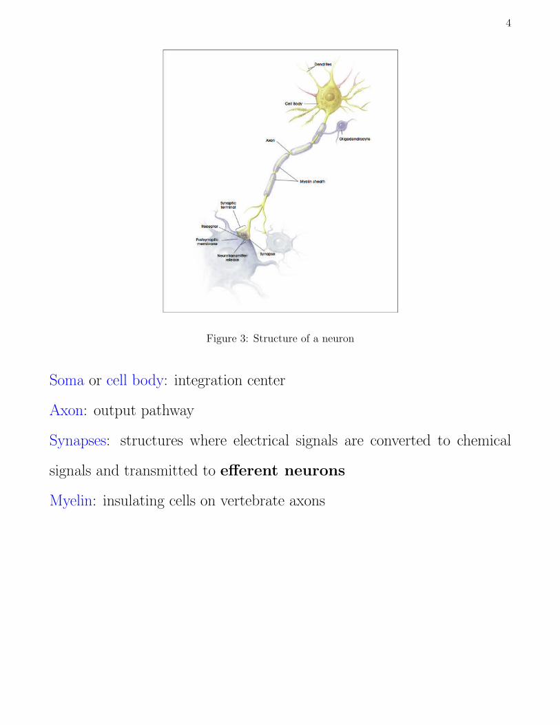
Figure 3: Structure of a neuron

Soma or cell body: integration center

Axon: output pathway

Synapses: structures where electrical signals are converted to chemical

signals and transmitted to efferent neurons

Myelin: insulating cells on vertebrate axons

5

Neurons often encode information in the frequency of spiking, or elec-

trical impulse firing rate. How are electricity and the neuron related?

Answer: ion channels.

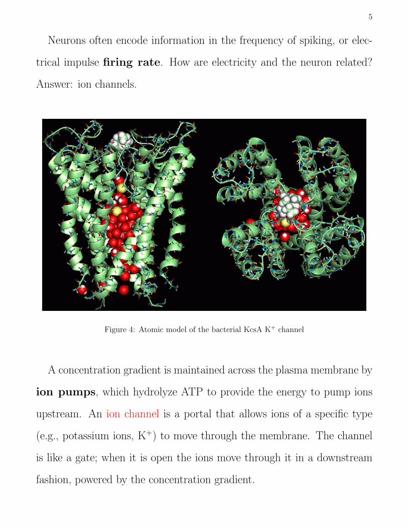
Figure 4: Atomic model of the bacterial KcsA K+ channel

A concentration gradient is maintained across the plasma membrane by

ion pumps, which hydrolyze ATP to provide the energy to pump ions

upstream. An ion channel is a portal that allows ions of a specific type

(e.g., potassium ions, K+) to move through the membrane. The channel

is like a gate; when it is open the ions move through it in a downstream

fashion, powered by the concentration gradient.

6

plasmamembranechannel

KCl

KCl

K +

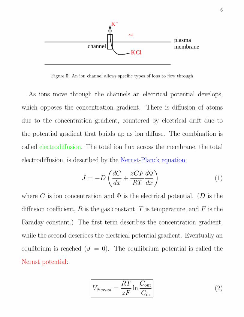
Figure 5: An ion channel allows specific types of ions to flow through

As ions move through the channels an electrical potential develops,

which opposes the concentration gradient. There is diffusion of atoms

due to the concentration gradient, countered by electrical drift due to

the potential gradient that builds up as ion diffuse. The combination is

called electrodiffusion. The total ion flux across the membrane, the total

electrodiffusion, is described by the Nernst-Planck equation:

J = −D(dC

dx+zCF

RT

dΦ

dx

)(1)

where C is ion concentration and Φ is the electrical potential. (D is the

diffusion coefficient, R is the gas constant, T is temperature, and F is the

Faraday constant.) The first term describes the concentration gradient,

while the second describes the electrical potential gradient. Eventually an

equlibrium is reached (J = 0). The equilibrium potential is called the

Nernst potential:

VNernst =RT

zFlnCout

Cin(2)

7

where VNernst = Φin − Φout and z is the ion valence. Typically,

[K+]in > [K+]out (3)

so VK < 0,

[Na+]in < [Na+]out (4)

and

[Ca2+]in < [Ca2+]out (5)

so VNa, VCa > 0. In fact, typical values are:

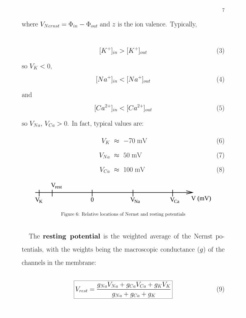
VK ≈ −70 mV (6)

VNa ≈ 50 mV (7)

VCa ≈ 100 mV (8)

VK

Vrest

0 V (mV)VNa VCa

Figure 6: Relative locations of Nernst and resting potentials

The resting potential is the weighted average of the Nernst po-

tentials, with the weights being the macroscopic conductance (g) of the

channels in the membrane:

Vrest =gNaVNa + gCaVCa + gKVK

gNa + gCa + gK(9)

8

Here, macroscopic conductance reflects the permeability of an ion type

through all open channels permeable to that ion type. For example, gCa

is the total permeability of Ca2+ through all open Ca2+ channels.

An Equivalent Circuit Description

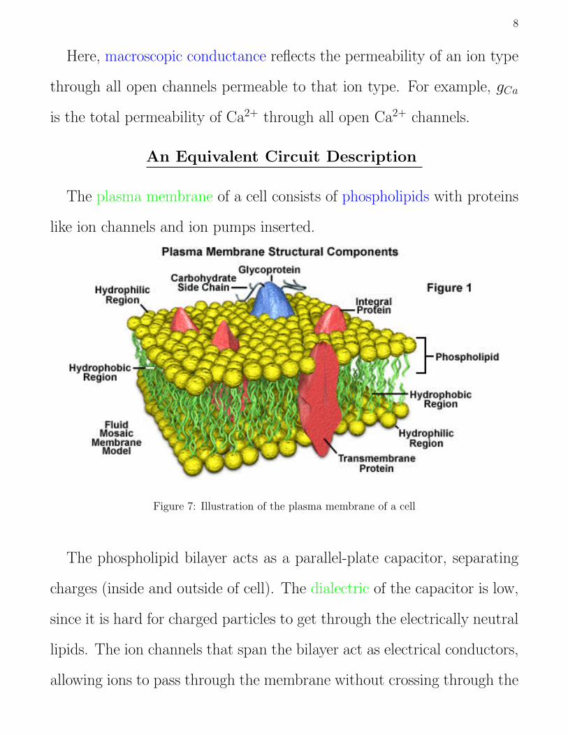
The plasma membrane of a cell consists of phospholipids with proteins

like ion channels and ion pumps inserted.

Figure 7: Illustration of the plasma membrane of a cell

The phospholipid bilayer acts as a parallel-plate capacitor, separating

charges (inside and outside of cell). The dialectric of the capacitor is low,

since it is hard for charged particles to get through the electrically neutral

lipids. The ion channels that span the bilayer act as electrical conductors,

allowing ions to pass through the membrane without crossing through the

9

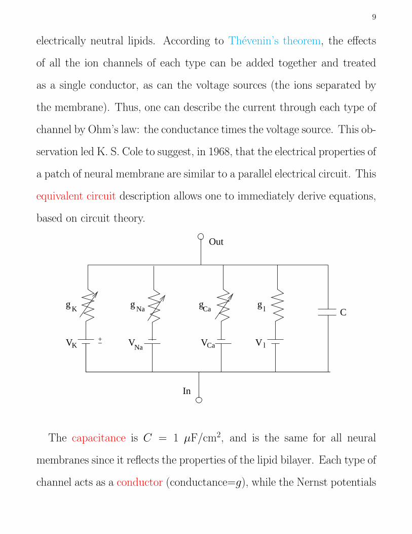
electrically neutral lipids. According to Thevenin’s theorem, the effects

of all the ion channels of each type can be added together and treated

as a single conductor, as can the voltage sources (the ions separated by

the membrane). Thus, one can describe the current through each type of

channel by Ohm’s law: the conductance times the voltage source. This ob-

servation led K. S. Cole to suggest, in 1968, that the electrical properties of

a patch of neural membrane are similar to a parallel electrical circuit. This

equivalent circuit description allows one to immediately derive equations,

based on circuit theory.

VK CaNaV lV

gK gNa gCa g l C

Out

In

+− V

The capacitance is C = 1 µF/cm2, and is the same for all neural

membranes since it reflects the properties of the lipid bilayer. Each type of

channel acts as a conductor (conductance=g), while the Nernst potentials

10

provide ionic driving forces. Each conductor, with the exception of the

leak, changes with the membrane potential. That is, each is rectifying.

The leak conductance is largely due to Cl− leaking through the various

channels. (Most neurons don’t have Cl− channels, although some do.)

Typically, the Cl− concentration is highest on the outside, and since the

valence is −1, Vl < 0.

We now use several laws from physics to derive the voltage equation.

First, by Ohm’s law,

V = IR (10)

where V is the voltage (membrane potential in the case of neurons), I is

the current, and R is resistance. But conductance = 1/resistance, so

I = gV . (11)

We modify this by noting that the current through, say, a K+ channel is

0 when V = VK , not when V = 0. Hence, in general,

I = g(V − VNernst) . (12)

Thus,

IK = gK(V − VK) (13)

INa = gNa(V − VNa) (14)

ICa = gCa(V − VCa) (15)

Il = gl(V − Vl) . (16)

11

In almost all cases, the membrane potential will be greater than VK

and less than VNa or VCa (the only exception would be under pathological

conditions or in in vitro brain slice experiments where one could move

the membrane potential to almost any value by injection current into the

neuron). Thus, in all physiological cases,

IK > 0 (17)

INa < 0 (18)

ICa < 0 (19)

and Il could be positive or negative. A positive current makes the voltage

more negative, and is called hyperpolarizing. A negative makes the voltage

less negative and is called depolarizing. These terms stem from the fact

that a circuit with a non-zero voltage is said to be polarized. So a resting

neuron, with V ≈ −70 mV is polarized, and making voltage any lower is

hyperpolarizing, making it closer to 0 is depolarizing.

These describe the currents through the ion channels. All current pass-

ing through the membrane either charges or discharges the membrane

capacitance. So the rate of change of charge on the membrane dq/dt is

the same as the net current flowing through the membrane:

I =dq

dt. (20)

12

But for a capacitor

q = CV (21)

sodq

dt= C

dV

dt(22)

and thus

Ic = CdV

dt(23)

is the capacitive current.

We combine the currents through the different branches of the parallel

circuit using Kirchoff’s current law. This states that the total charge

through a circuit must be conserved, and in the case of a parallel circuit

the sum of the currents through the different branches must equal 0. Thus,

Ic + IK + INa + ICa + Il = 0 . (24)

Rewriting,

Ic = −(IK + INa + ICa + Il) (25)

ordV

dt= −(IK + INa + ICa + Il)/C (26)

This is the Voltage Equation.

Since each ionic current is linear in V when the conductances are con-

stant, this is a linear ODE. In this case,

dV

dt= (−aV + b)/C (27)

13

where a is the sum of the ionic conductances and b is the sum of the

Nernst potentials weighted by the conductances. (If we set dVdt = 0 to get

the equilibrium voltage this comes out to be the resting potential, Eq. 9.)

This can be rewritten as

dV

dt= (V∞ − V )/τv (28)

where V∞ = ba is the equilibrium potential or resting potential Vrest and

τv = Ca is the membrane time constant. The solution to a linear ODE of

this form is:

V (t) = V∞ + (V0 − V∞)e−t/τv. (29)

where V0 is the initial voltage. Thus, if V is perturbed from rest to some

value V0 then it will return to rest exponentially. If the time constant τv

is large then the return to rest is slow, if small then the return to rest is

rapid.

What happens if some external current is applied? Then while that

current is on the equilibrium voltage will change from Vrest to some new

equilibrium V∞. The input resistance is then defined as

Rin =V∞ − Vrest

Iap(30)

where Iap is the applied current. In practice, the input resistance is deter-

mined by injecting a small applied current and measuring the new equilib-

rium potential. Small injected currents are used since for small deviations

14

from rest the conductances are approximately constant (as we shall see,

for larger depolarizing deviations the conductances change).

There is a reciprocal relationship between resistance and conductance,

so

gin =1

Rin(31)

and if the conductances are constant, then

gin = gK + gNa + gCa + gL = a . (32)

Thus,

τv =C

gin(33)

and so

τv = RinC . (34)

In practice, this formula is used to calculate the membrane time constant,

after first measuring Rin and the capacitance C.

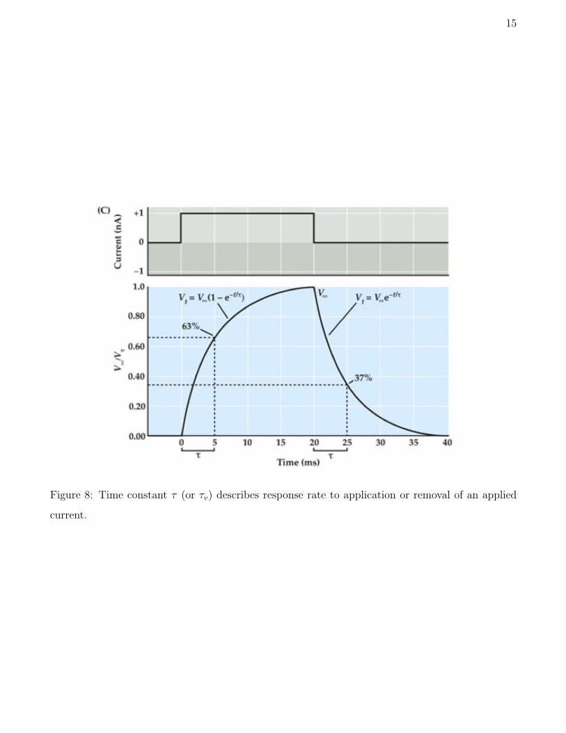
The membrane time canstant tells us how fast the membrane potential

responds to an applied current. It is roughly the time required to reach

two thirds of the way from the original voltage to the new equilibrium

voltage.

ELECTRICAL EXCITABILITY

If the conductances were constant, then the neuron would act like a

passive resister in parallel with a capacitor. However, the conductances

15

Figure 8: Time constant τ (or τv) describes response rate to application or removal of an applied

current.

16

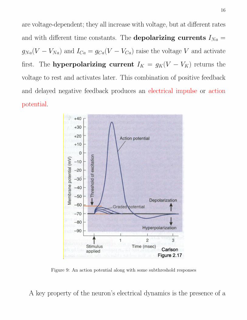
are voltage-dependent; they all increase with voltage, but at different rates

and with different time constants. The depolarizing currents INa =

gNa(V − VNa) and ICa = gCa(V − VCa) raise the voltage V and activate

first. The hyperpolarizing current IK = gK(V − VK) returns the

voltage to rest and activates later. This combination of positive feedback

and delayed negative feedback produces an electrical impulse or action

potential.

Figure 9: An action potential along with some subthreshold responses

A key property of the neuron’s electrical dynamics is the presence of a

17

threshold. Voltage perturbations above this threshold evoke an impulse.

The conductance of an ionic current is the product of the single-channel

conductance and the number of open channels. The single-channel con-

ductance is roughly constant, while the number of open channels depends

on the membrane potential. Let g denote the maximum conductance,

i.e., the single-channel conductance times the total number of channels of

a single type. Then

g = g Prob[channel open] . (35)

To determine this probability function (which depends on V ), Alan

Hodgkin and Andrew Huxley used the squid giant axon as a model

system. This is a large axon (up to 1 mm in diameter) that controls part

of the squid’s water jet propulsion system. Because it is large, it is fairly

easy to work with.

The technique that Hodgkin-Huxley used to determine Prob[channel open]

is the voltage clamp. This acts like a thermostat, injecting the right

amount of current to hold the potential at any value of V desired. The

injected current is the negative of the current generated by the axon at

this voltage. If all currents other than, say, K+ current, are blocked phar-

macologically, then

Icmp = −g(Vcmp)(Vcmp − VK) (36)

18

so that

g(Vcmp) =−Icmp

Vcmp − VK. (37)

This can be done for a range of clamping voltages to obtain the g(V )

function.The g parameter is just g(V ) at a high (saturating) voltage. Then

Prob[channel open] = g(V )/g . (38)

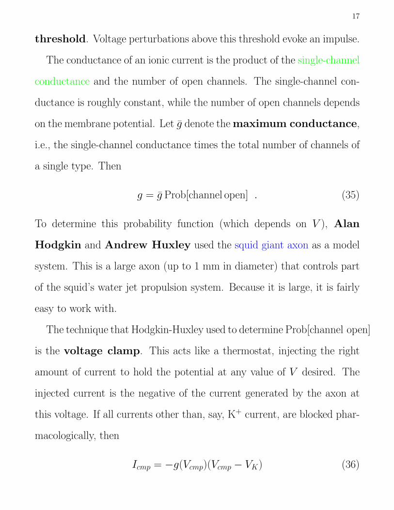
Using this approach, H-H found that the best fit is

Prob[channel open] = n4∞(V ) (39)

where n∞(V ) is a sigmoid function:

V

n1

Figure 10: Sigmoidal n∞ function.

The equation for this is

n∞(V ) = 0.5

[1 + tanh

(V − V1

s1

)](40)

which can be re-written as

n∞(V ) =eu

eu + e−u(41)

19

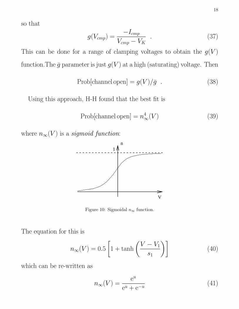
where u = V−V1s1

with parameters V1 and s1 > 0 that modify the shape of

the function (I call them shape parameters). By raising n∞ to the fourth

power, the curve is sharpened:

V

n1

n4

Figure 11: Curve is sharpened by raising n∞ to an integer power.

This is a steady state description of the channel open probability, but

this probability (or channel open fraction) changes over time as it ap-

proaches its steady state. Thus,

Prob[potassium channel open] = n4 . (42)

where n is described by a differential equation. This variable, which

satisfies n ∈ [0, 1], is called an activation variable. It’s time dynamics are

described bydn

dt=n∞(V )− nτn(V )

(43)

which says that if n is smaller than its equilibrium value n∞(V ) then

dndt > 0 so n will increase toward n∞(V ). The bigger the difference between

the current value of n and its equilibrium value the faster n will move

20

towards n∞. Also, the speed is regulated by the time constant τn; if τn is

large then n will move slowly towards n∞. Note that both the equilibrium

function n∞ and the time constant τn depend of the membrane potential

V .

The K+ conductance is then

gK = gK n4 (44)

and the K+ current is

IK = gK n4(V − VK) . (45)

What is n physically? Hodgkin and Huxley thought of the K+ channel

as composed of 4 independent gates, each of which must be open for the

channel to be open. Then n represents the probability that one of the

gates is open. This is not an accurate description (as we know today), but

intuitively it is very helpful.

The Na+ channel is more complicated, since now there is an inactivation

gate as well as activation gates. This gate is the opposite of an activation

gate, it closes when V is depolarized. Let

h = Prob[inactivation gate open] . (46)

There is also an activation gate, denoted by m, which is qualitatively

similar to n:

m = Prob[activation gate open] . (47)

21

The differential equations for the time dynamics of the activation variable

m and inactivation variable h are:

dm

dt=

m∞(V )−mτm(V )

(48)

dh

dt=

h∞(V )− hτh(V )

(49)

According to the Hodgkin-Huxley data fitting,

gNa = gNam3h (50)

which intuitively means that 3 activation gates and 1 inactivation gate

must be open for the channel to be open. Then,

INa = gNam3h(V − VNa) (51)

is the Na+ current.

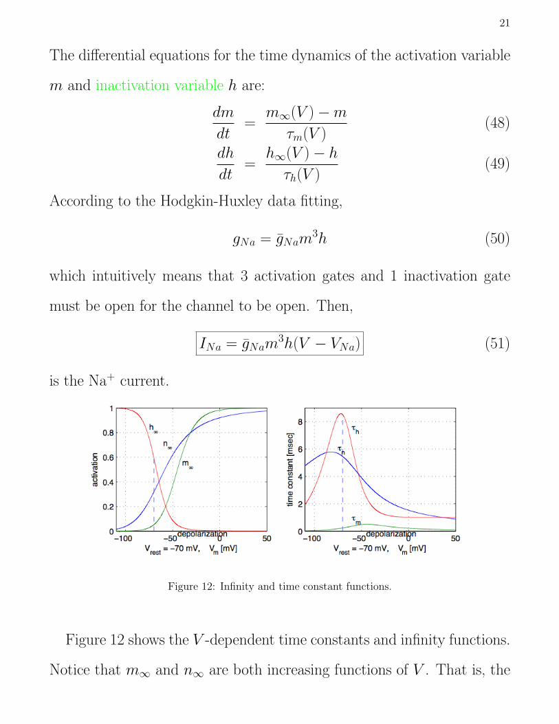
Figure 12: Infinity and time constant functions.

Figure 12 shows the V -dependent time constants and infinity functions.

Notice that m∞ and n∞ are both increasing functions of V . That is, the

22

activation gates open when the membrane is depolarized. In contrast, h∞

is a decreasing function of voltage. That is, the inactivation gate closes

when the membrane is depolarized. The time constant functions are all

bell-shaped; they are low at very hyperpolarized and depolarized voltages,

and larger in between.

An important property of the two types of gate in the Na+ current is

that the activation time constant is smaller than the inactivation time con-

stant (Fig. 12), so that when the membrane is depolarized the activation

gates open first. This turns on the Na+ current, causing voltage to rise

further. It is only later that the inactivation gates close. So the current

provides rapid positive feedback followed by a delayed negative feedback.

The K+ current provides only delayed negative feedback.

The last current in the Hodgkin-Huxley model is a constant-conductance

leak current. This is due largely to non-specific flow of ions across the

membrane through various channel types. The important feature here is

that the conductance is not a function of V . The leak Nernst potential is

usually about VL = −40 mV, so the current is mildly depolarizing. Then

IL = gL(V − VL) (52)

23

Combining previous equations, we get the full Hodgkin-Huxley model:

dV

dt= −[gNam

3h(V − VNa) + gKn4(V − VK) + gL(V − VL)]/C (53)

dn

dt= [n∞(V )− n]/τn(V ) (54)

dm

dt= [m∞(V )−m]/τm(V ) (55)

dh

dt= [h∞(V )− h]/τh(V ) . (56)

The Hodgkin-Huxley model was developed to explain how action poten-

tials are produced. The biophysical concept, implemented mathematically

in the model, is described below.

24

Response to Input

Input to nerve cells comes primarily through synaptic connections that

link neurons together. At these synapses the electrical signal (electrical

impulses) is transduced to a chemical signal through the release or ex-

ocytosis of neurotransmitter molecules. The neurotransmitter diffuses

across the space between presynaptic and postsynaptic neurons, called the

synaptic cleft, and binds to receptors on the postsynaptic membrane. This

induces the opening of ion channels, which could either be the postsynap-

tic receptor itself or other channels activated by the receptor, allowing

ionic current to flow. Thus, the input is ultimately an ionic current.

In the lab one can mimic this by applying current to the cell directly

with an electrode. In terms of the equations, one simply modifies the

voltage equation by adding a term for the applied current, Iap:

dV

dt= −(INa + IK + IL − Iap)/C (57)

where the minus sign is used for Iap so that a positive applied current

results in depolarization.

Threshold effect: The H-H model exhibits a threshold response to

applied current. If a square pulse of current is applied and the magnitude

and duration of the pulse is too small, then the system will have a passive

or subthreshold response. If the input pulse is sufficiently large, then the

25

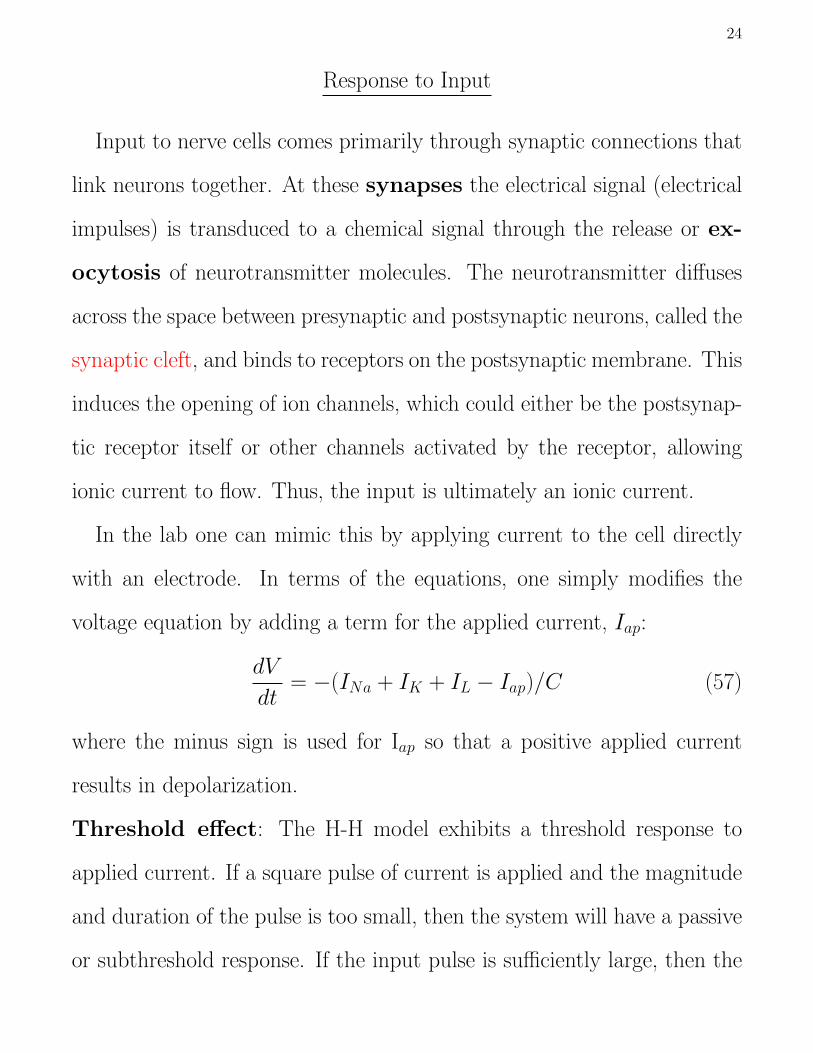
system will produce an impulse. So the output is all-or-none (Fig. 13).

V (mV)

t (ms)

t (ms)

Iap

Figure 13: The H-H model produces a passive or subthreshold response if the current pulse is small,

or an impulse if the pulse is large enough.

Firing rate and gain function: If applied current is maintained con-

tinuously, then the system may either produce a single impulse and then

come to rest at a more depolarized voltage, or it may spike continuously

if Iap is sufficiently large (in this case, Iap > 6 µA/cm2). In the H-H

model this spike train will be periodic, with some period T . The firing

rate is then ν = 1T . The gain function is ν as a function of Iap. For the

H-H model, the spike frequency increases as the applied current increases

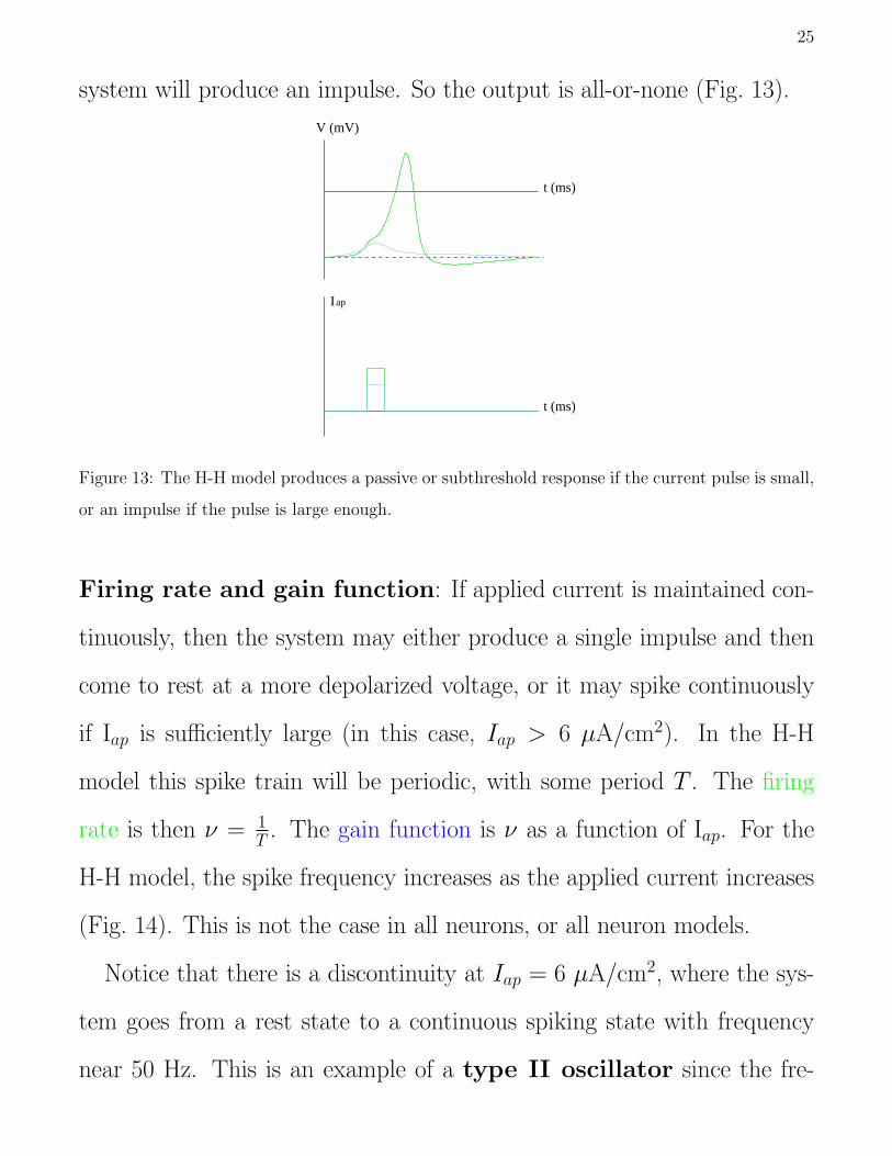
(Fig. 14). This is not the case in all neurons, or all neuron models.

Notice that there is a discontinuity at Iap = 6 µA/cm2, where the sys-

tem goes from a rest state to a continuous spiking state with frequency

near 50 Hz. This is an example of a type II oscillator since the fre-

26

Iap

ν (Hz)

50

6

Figure 14: Gain function for the H-H model.

quency did not approach 0. We return to this later.

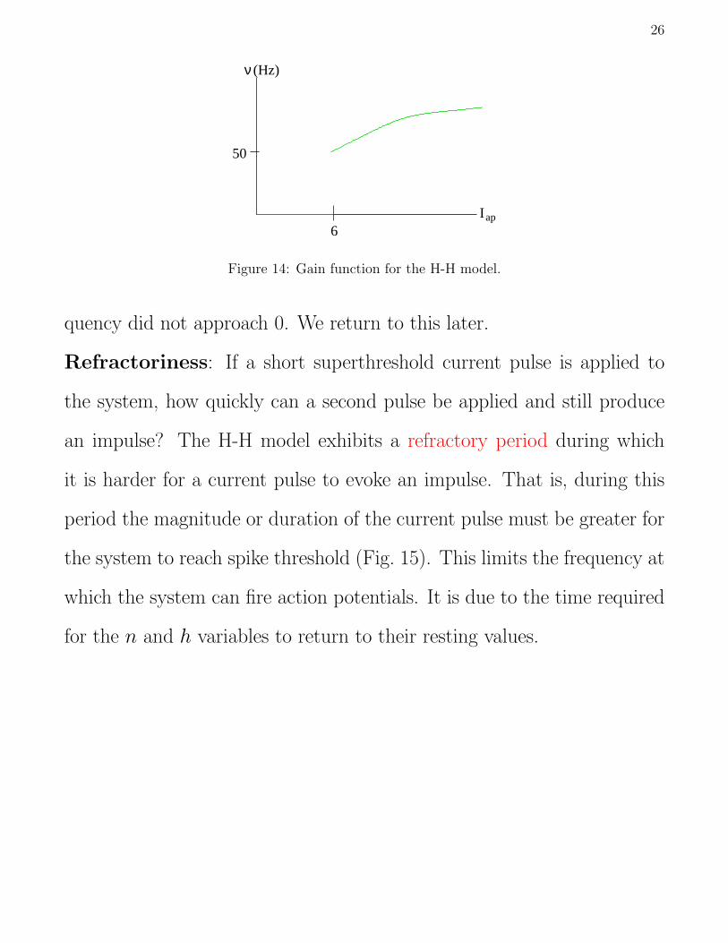
Refractoriness: If a short superthreshold current pulse is applied to

the system, how quickly can a second pulse be applied and still produce

an impulse? The H-H model exhibits a refractory period during which

it is harder for a current pulse to evoke an impulse. That is, during this

period the magnitude or duration of the current pulse must be greater for

the system to reach spike threshold (Fig. 15). This limits the frequency at

which the system can fire action potentials. It is due to the time required

for the n and h variables to return to their resting values.

27

time after first stimulus (ms)

apI

refractory

Figure 15: Magnitude of the Iap pulse required to bring the system to threshold following an initial

suprathreshold stimulus.

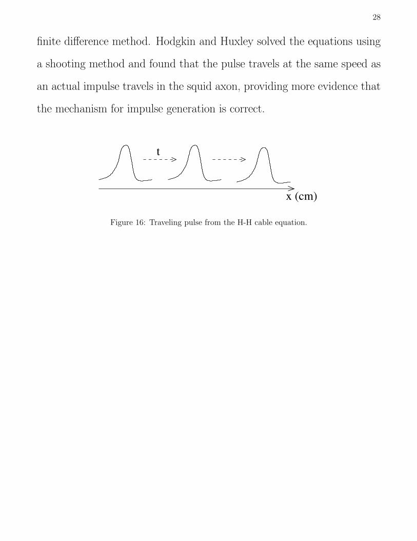
Traveling Pulse

The H-H model describes the electrical activity of a space clamped

axon, where a wire is run through the center of the axon to maintain

uniform potential. Physiologically, an impulse is typically generated in

the soma or the axon hillock (initial portion of the axon) and travels

down the axon by exciting adjacent portions of membrane. It travels

down the axon without dissipation, unlike water waves that attenuate as

they travel. This is called a traveling pulse or a soliton and is described

mathematically by the Hodgkin-Huxley cable equation:

C∂V

∂t=

a

2R

∂2V

∂x2− [INa + IK + IL − Iap] (58)

where a is the axon radius and R is the lateral resistivity. There are

also the usual ODEs for the activation and inactivation variables. This

system of partial and ordinary DEs could be solved numerically using a

28

finite difference method. Hodgkin and Huxley solved the equations using

a shooting method and found that the pulse travels at the same speed as

an actual impulse travels in the squid axon, providing more evidence that

the mechanism for impulse generation is correct.

x (cm)

t

Figure 16: Traveling pulse from the H-H cable equation.