Rigid Motion and Homogeneous Transformations

Chapter 2

RIGID MOTIONS ANDHOMOGENEOUSTRANSFORMATIONS

A large part of robot kinematics is concerned with the establishment ofvarious coordinate systems to represent the positions and orientations ofrigid objects and with transformations among these coordinate systems.Indeed, the geometry of three-dimensional space and of rigid motions playsa central role in all aspects of robotic manipulation. In this chapter westudy the operations of rotation and translation and introduce the notionof homogeneous transformations.1 Homogeneous transformations combinethe operations of rotation and translation into a single matrix multiplication,and are used in Chapter 3 to derive the so-called forward kinematic equationsof rigid manipulators.

We begin by examining representations of points and vectors in a Eu-clidean space equipped with multiple coordinate frames. Following this, wedevelop the concept of a rotation matrix, which can be used to representrelative orientations between coordinate frames. Finally, we combine thesetwo concepts to build homogeneous transformation matrices, which can beused to simultaneously represent the position and orientation of one coordi-nate frame relative to another. Furthermore, homogeneous transformationmatrices can be used to perform coordinate transformations. Such trans-formations allow us to easily move between different coordinate frames, afacility that we will often exploit in subsequent chapters.

1Since we make extensive use of elementary matrix theory, the reader may wish toreview Appendix A before beginning this chapter.

37

38CHAPTER 2. RIGID MOTIONS AND HOMOGENEOUS TRANSFORMATIONS

��

��

� �

��

��

�

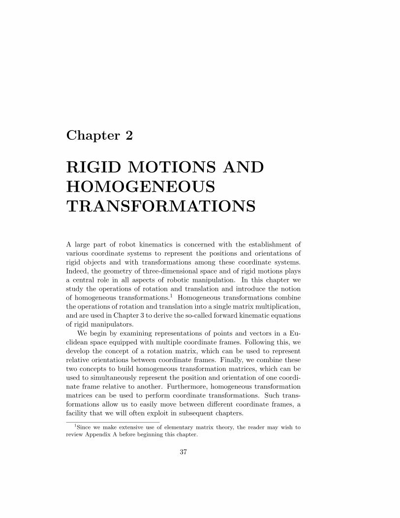
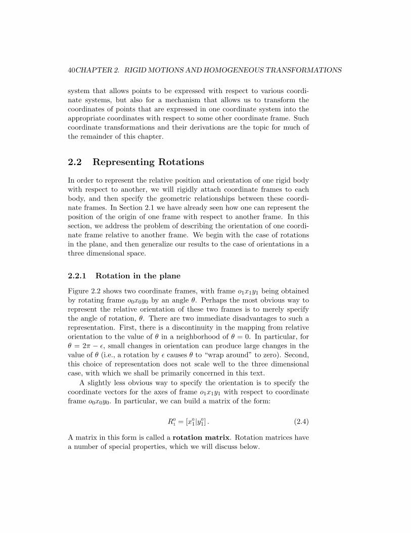
Figure 2.1: Two coordinate frames, a point p, and two vectors ~v1 and ~v2.

2.1 Representing Positions

Before developing representation schemes for points and vectors, it is instruc-tive to distinguish between the two fundamental approaches to geometricreasoning: the synthetic approach and the analytic approach. In the former,one reasons directly about geometric entities (e.g., points or lines), while inthe latter, one represents these entities using coordinates or equations, andreasoning is performed via algebraic manipulations.

Consider Figure 2.1. Using the synthetic approach, without ever assign-ing coordinates to points or vectors, one can say that x0 is perpendicularto y0, or that ~v1 × ~v2 defines a vector that is perpendicular to the planecontaining ~v1 and ~v2, in this case pointing out of the page.

In robotics, one typically uses analytic reasoning, since robot tasks areoften defined in a Cartesian workspace, using Cartesian coordinates. Ofcourse, in order to assign coordinates it is necessary to specify a coordinateframe. Consider again Figure 2.1. We could specify the coordinates of thepoint p with respect to either frame o0x0y0 or frame o1x1y1. In the formercase, we might assign to p the coordinate vector (5, 6)T , and in the latter case(−3, 4)T . So that the reference frame will always be clear, we will adopt anotation in which a superscript is used to denote the reference frame. Thus,we would write

p0 =

[

56

]

, p1 =

[

−34

]

(2.1)

Geometrically, a point corresponds to a specific location in space. Westress here that p 6= p0 and p 6= p1, i.e., p is a geometric entity, a pointin space, while both p0 and p1 are coordinate vectors that represent the

2.1. REPRESENTING POSITIONS 39

location of this point in space with respect to coordinate frames o0x0y0 ando1x1y1, respectively.

Since the origin of a coordinate system is just a point in space, we canassign coordinates that represent the position of the origin of one coordinatesystem with respect to another. In Figure 2.1, for example,

o0

1=

[

105

]

, o1

0=

[

−105

]

. (2.2)

In cases where there is only a single coordinate frame, or in which thereference frame is obvious, we will often omit the superscript. This is a slightabuse of notation, and the reader is advised to bear in mind the differencebetween the geometric entity called p and any particular coordinate vectorthat is assigned to represent p. The former is invariant with respect tothe choice of coordinate systems, while the latter obviously depends on thechoice of coordinate frames.

While a point corresponds to a specific location in space, a vector specifiesa direction and a magnitude. Vectors can be used, for example, to representdisplacements or forces. Therefore, while the point p is not equivalent tothe vector ~v1, the displacement from the origin o0 to the point p is givenby the vector ~v1. In this text, we will use the term vector to refer to whatare sometimes called free vectors, i.e., vectors that are not constrained to belocated at a particular point in space. Under this convention, it is clear thatpoints and vectors are not equivalent, since points refer to specific locationsin space, but a vector can be moved to any location in space. Under thisconvention, two vectors are equal if they have the same direction and thesame magnitude.

When assigning coordinates to vectors, we use the same notational con-vention that we used when assigning coordinates to points. Thus, ~v1 and~v2 are geometric entities that are invariant with respect to the choice ofcoordinate systems, but the representation by coordinates of these vectorsdepends directly on the choice of reference coordinate frame. In the exampleof Figure 2.1, we would obtain

v0

1 =

[

56

]

, v1

1 =

[

81

]

, v0

2 =

[

−51

]

v1

2 =

[

−34

]

. (2.3)

In order to perform algebraic manipulations using coordinates, it is es-sential that all coordinate vectors be defined with respect to the same coordi-nate frame. For example, an expression of the form v1

1 + v2

2 would make nosense geometrically. Thus, we see a clear need, not only for a representation


system that allows points to be expressed with respect to various coordi-nate systems, but also for a mechanism that allows us to transform thecoordinates of points that are expressed in one coordinate system into theappropriate coordinates with respect to some other coordinate frame. Suchcoordinate transformations and their derivations are the topic for much ofthe remainder of this chapter.

2.2 Representing Rotations

In order to represent the relative position and orientation of one rigid bodywith respect to another, we will rigidly attach coordinate frames to eachbody, and then specify the geometric relationships between these coordi-nate frames. In Section 2.1 we have already seen how one can represent theposition of the origin of one frame with respect to another frame. In thissection, we address the problem of describing the orientation of one coordi-nate frame relative to another frame. We begin with the case of rotationsin the plane, and then generalize our results to the case of orientations in athree dimensional space.

2.2.1 Rotation in the plane

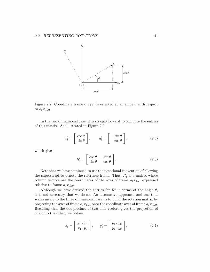
Figure 2.2 shows two coordinate frames, with frame o1x1y1 being obtainedby rotating frame o0x0y0 by an angle θ. Perhaps the most obvious way torepresent the relative orientation of these two frames is to merely specifythe angle of rotation, θ. There are two immediate disadvantages to such arepresentation. First, there is a discontinuity in the mapping from relativeorientation to the value of θ in a neighborhood of θ = 0. In particular, forθ = 2π − ǫ, small changes in orientation can produce large changes in thevalue of θ (i.e., a rotation by ǫ causes θ to “wrap around” to zero). Second,this choice of representation does not scale well to the three dimensionalcase, with which we shall be primarily concerned in this text.

A slightly less obvious way to specify the orientation is to specify thecoordinate vectors for the axes of frame o1x1y1 with respect to coordinateframe o0x0y0. In particular, we can build a matrix of the form:

R0

1= [x0

1|y0

1] . (2.4)

A matrix in this form is called a rotation matrix. Rotation matrices havea number of special properties, which we will discuss below.

2.2. REPRESENTING ROTATIONS 41

o0, o1

y0

y1

θ

x1

sin θ

cos θ

x0

Figure 2.2: Coordinate frame o1x1y1 is oriented at an angle θ with respectto o0x0y0

In the two dimensional case, it is straightforward to compute the entriesof this matrix. As illustrated in Figure 2.2,

x0

1 =

[

cos θsin θ

]

, y0

1 =

[

− sin θcos θ

]

, (2.5)

which gives

R0

1=

[

cos θ − sin θsin θ cos θ

]

. (2.6)

Note that we have continued to use the notational convention of allowingthe superscript to denote the reference frame. Thus, R0

1is a matrix whose

column vectors are the coordinates of the axes of frame o1x1y1 expressedrelative to frame o0x0y0.

Although we have derived the entries for R0

1in terms of the angle θ,

it is not necessary that we do so. An alternative approach, and one thatscales nicely to the three dimensional case, is to build the rotation matrix byprojecting the axes of frame o1x1y1 onto the coordinate axes of frame o0x0y0.Recalling that the dot product of two unit vectors gives the projection ofone onto the other, we obtain

x0

1 =

[

x1 · x0

x1 · y0

]

, y0

1 =

[

y1 · x0

y1 · y0

]

, (2.7)


which can be combined to obtain the rotation matrix

R0

1=

[

x1 · x0 y1 · x0

x1 · y0 y1 · y0

]

. (2.8)

Thus the columns of R0

1specify the direction cosines of the coordinate axes

of o1x1y1 relative to the coordinate axes of o0x0y0. For example, the firstcolumn (x1 · x0, x1 · y0)

T of R0

1specifies the direction of x1 relative to the

frame o0x0y0. Note that the right hand sides of these equations are defined interms of geometric entities, and not in terms of their coordinates. ExaminingFigure 2.2 it can be seen that this method of defining the rotation matrixby projection gives the same result as was obtained in equation (2.6).

If we desired instead to describe the orientation of frame o0x0y0 withrespect to the frame o1x1y1 (i.e., if we desired to use the frame o1x1y1 asthe reference frame), we would construct a rotation matrix of the form

R1

0=

[

x0 · x1 y0 · x1

x0 · y1 y0 · y1

]

. (2.9)

Since the inner product is commutative, (i.e. xi · yj = yj · xi), we see that

R1

0= (R0

1)T . (2.10)

In a geometric sense, the orientation of o0x0y0 with respect to the frameo1x1y1 is the inverse of the orientation of o1x1y1 with respect to the frameo0x0y0. Algebraically, using the fact that coordinate axes are always mutu-ally orthogonal, it can readily be seen that

(R0

1)T = (R0

1)−1. (2.11)

Such a matrix is said to be orthogonal. The column vectors of R0

1

are of unit length and mutually orthogonal (Problem 2-1). It can also beshown (Problem 2-2) that detR0

1= ±1. If we restrict ourselves to right-

handed coordinate systems, as defined in Appendix A, then detR0

1= +1

(Problem 2-3). All rotation matrices have the properties of being orthogonalmatrices with determinant +1. It is customary to refer to the set of all 2×2rotation matrices by the symbol SO(2)2. The properties of such matricesare summarized in Figure 2.3.

To provide further geometric intuition for the notion of the inverse of arotation matrix, note that in the two dimensional case, the inverse of the

2The notation SO(2) stands for Special Orthogonal group of order 2.

2.2. REPRESENTING ROTATIONS 43

Every n× n rotation matrix R has the following properties (for n = 2, 3):

• R ∈ SO(n)

• R−1 ∈ SO(n)

• R−1 = RT

• The columns (and therefore the rows) of R are mutually orthogonal.

• Each column (and therefore each row) of R is a unit vector.

• det{R} = 1

Figure 2.3: Properties of Rotation Matrices

rotation matrix corresponding to a rotation by angle θ can also be easilycomputed simply by constructing the rotation matrix for a rotation by theangle −θ:

[

cos(−θ) − sin(−θ)sin(−θ) cos(−θ)

]

=

[

cos θ sin θ− sin θ cos θ

]

=

[


]T

.

(2.12)

2.2.2 Rotations in three dimensions

The projection technique described above scales nicely to the three dimen-sional case. In three dimensions, each axis of the frame o1x1y1z1 is projectedonto coordinate frame o0x0y0z0. The resulting rotation matrix is given by

R0

1=

x1 · x0 y1 · x0 z1 · x0

x1 · y1 y1 · y0 z1 · y0

x1 · z1 y1 · z0 z1 · z0

. (2.13)

As was the case for rotation matrices in two dimensions, matrices in thisform are orthogonal, with determinant equal to 1. In this case, 3×3 rotationmatrices belong to the group SO(3). The properties listed in Figure 2.3 alsoapply to rotation matrices in SO(3).

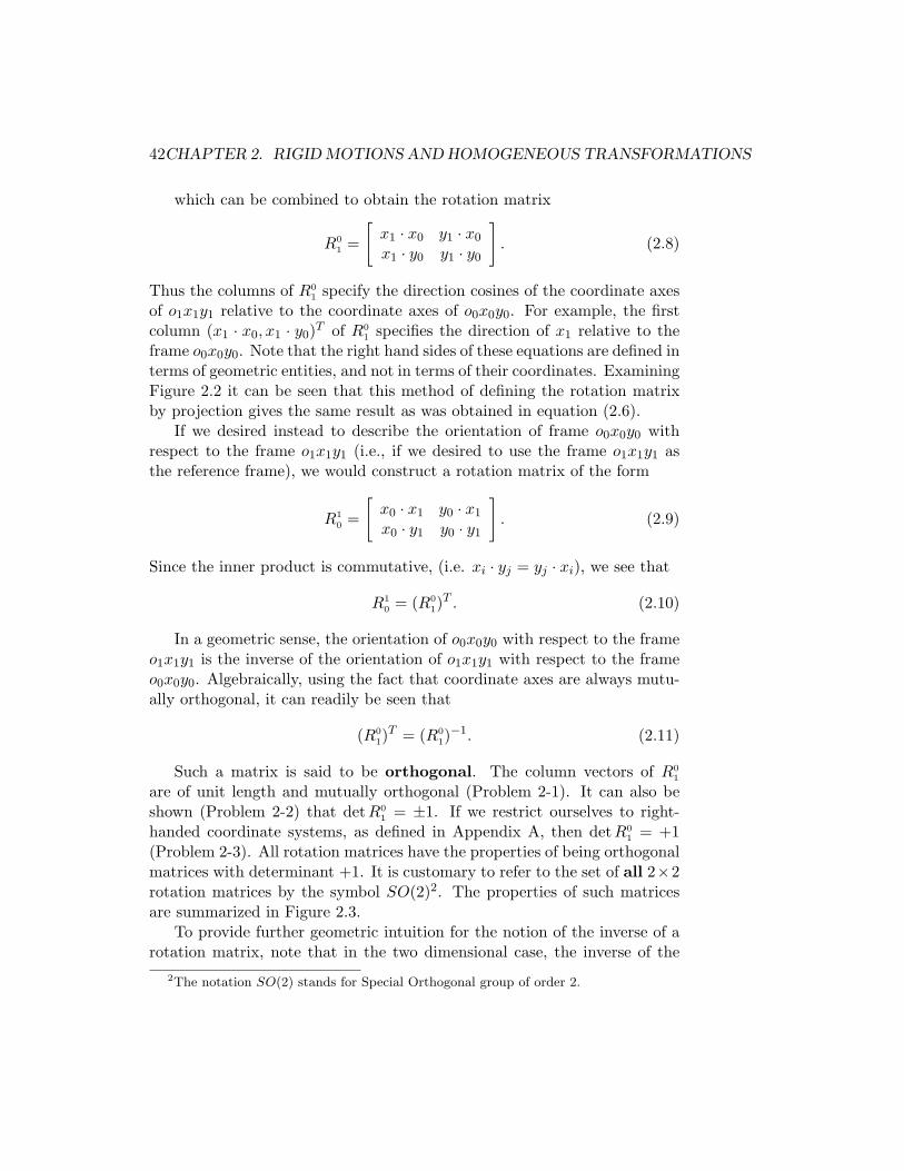
Example 2.1 Suppose the frame o1x1y1z1 is rotated through an angle θabout the z0-axis, and it is desired to find the resulting transformation matrix


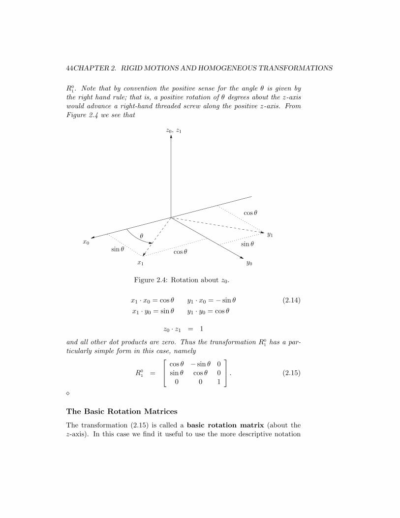
R0

1. Note that by convention the positive sense for the angle θ is given by

the right hand rule; that is, a positive rotation of θ degrees about the z-axiswould advance a right-hand threaded screw along the positive z-axis. FromFigure 2.4 we see that

y0

z0, z1

x0

y1

cos θ

sin θθ

cos θ

x1

sin θ

Figure 2.4: Rotation about z0.

x1 · x0 = cos θ y1 · x0 = − sin θ (2.14)

x1 · y0 = sin θ y1 · y0 = cos θ

z0 · z1 = 1

and all other dot products are zero. Thus the transformation R0

1has a par-

ticularly simple form in this case, namely

R0

1=

cos θ − sin θ 0sin θ cos θ 0

0 0 1

. (2.15)

⋄

The Basic Rotation Matrices

The transformation (2.15) is called a basic rotation matrix (about thez-axis). In this case we find it useful to use the more descriptive notation

2.3. COORDINATE TRANSFORMATIONS: ROTATIONS 45

Rz,θ, instead of R0

1to denote the matrix (2.15). It is easy to verify that the

basic rotation matrix Rz,θ has the properties

Rz,0 = I (2.16)

Rz,θRz,φ = Rz,θ+φ (2.17)

which together imply

Rz,θ

−1 = Rz,−θ. (2.18)

Similarly the basic rotation matrices representing rotations about the xand y-axes are given as (Problem 2-5)

Rx,θ =

1 0 00 cos θ − sin θ0 sin θ cos θ

(2.19)

Ry,θ =

cos θ 0 sin θ0 1 0

− sin θ 0 cos θ

(2.20)

which also satisfy properties analogous to (2.16)-(2.18).

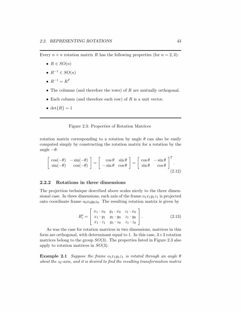
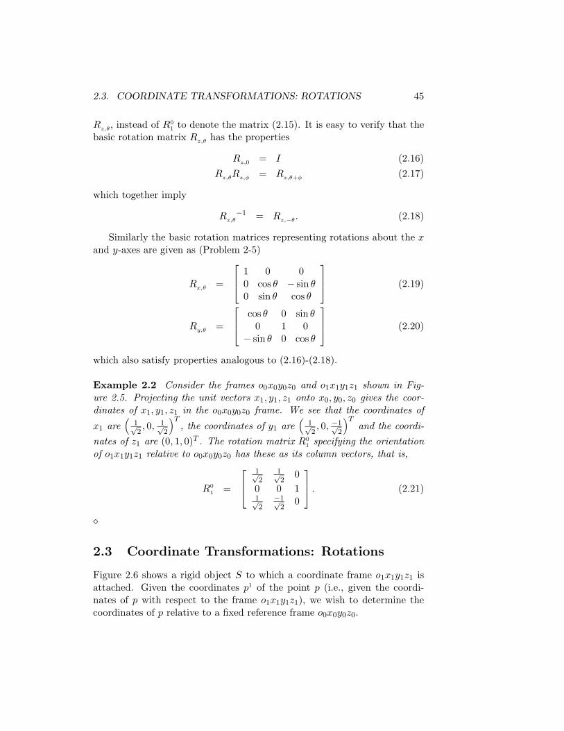
Example 2.2 Consider the frames o0x0y0z0 and o1x1y1z1 shown in Fig-ure 2.5. Projecting the unit vectors x1, y1, z1 onto x0, y0, z0 gives the coor-dinates of x1, y1, z1 in the o0x0y0z0 frame. We see that the coordinates of

x1 are(

1√2, 0, 1√

2

)T, the coordinates of y1 are

(

1√2, 0, −1√

2

)Tand the coordi-

nates of z1 are (0, 1, 0)T . The rotation matrix R0

1specifying the orientation

of o1x1y1z1 relative to o0x0y0z0 has these as its column vectors, that is,

R0

1=

1√2

1√2

0

0 0 11√2

−1√2

0

. (2.21)

⋄

2.3 Coordinate Transformations: Rotations

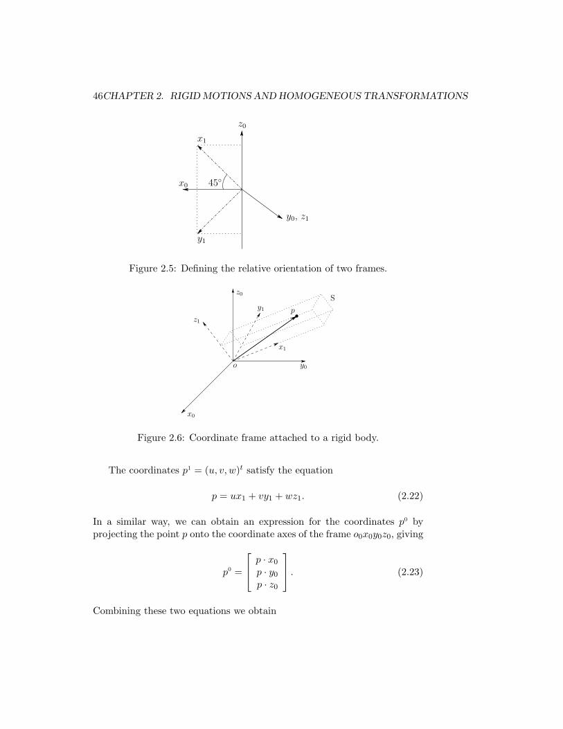
Figure 2.6 shows a rigid object S to which a coordinate frame o1x1y1z1 isattached. Given the coordinates p1 of the point p (i.e., given the coordi-nates of p with respect to the frame o1x1y1z1), we wish to determine thecoordinates of p relative to a fixed reference frame o0x0y0z0.


z0

x1

y1

y0, z1

45◦x0

Figure 2.5: Defining the relative orientation of two frames.

y1

z1

z0

x0

x1

o y0

S

p

Figure 2.6: Coordinate frame attached to a rigid body.

The coordinates p1 = (u, v, w)t satisfy the equation

p = ux1 + vy1 + wz1. (2.22)

In a similar way, we can obtain an expression for the coordinates p0 byprojecting the point p onto the coordinate axes of the frame o0x0y0z0, giving

p0 =

p · x0

p · y0

p · z0

. (2.23)

Combining these two equations we obtain


p0 =

(ux1 + vy1 + wz1) · x0

(ux1 + vy1 + wz1) · y0

(ux1 + vy1 + wz1) · z0

(2.24)

=

ux1 · x0 + vy1 · x0 + wz1 · x0

ux1 · y0 + vy1 · y0 + wz1 · y0

ux1 · z0 + vy1 · z0 + wz1 · z0

(2.25)

=

x1 · x0 y1 · x0 z1 · x0

x1 · y0 y1 · y0 z1 · y0

x1 · z0 y1 · z0 z1 · z0

u

v

w

. (2.26)

But the matrix in this final equation is merely the rotation matrix R0

1, which

leads top0 = R0

1p1. (2.27)

Thus, the rotation matrix R0

1can be used not only to represent the

orientation of coordinate frame o1x1y1z1 with respect to frame o0x0y0z0, butalso to transform the coordinates of a point from one frame to another. Thus,if a given point is expressed relative to o1x1y1z1 by coordinates p1, then R0

1p1

represents the same point expressed relative to the frame o0x0y0z0.We have now seen how rotation matrices can be used to relate the ori-

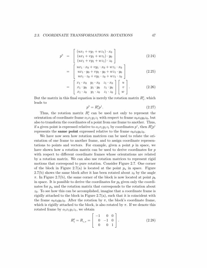
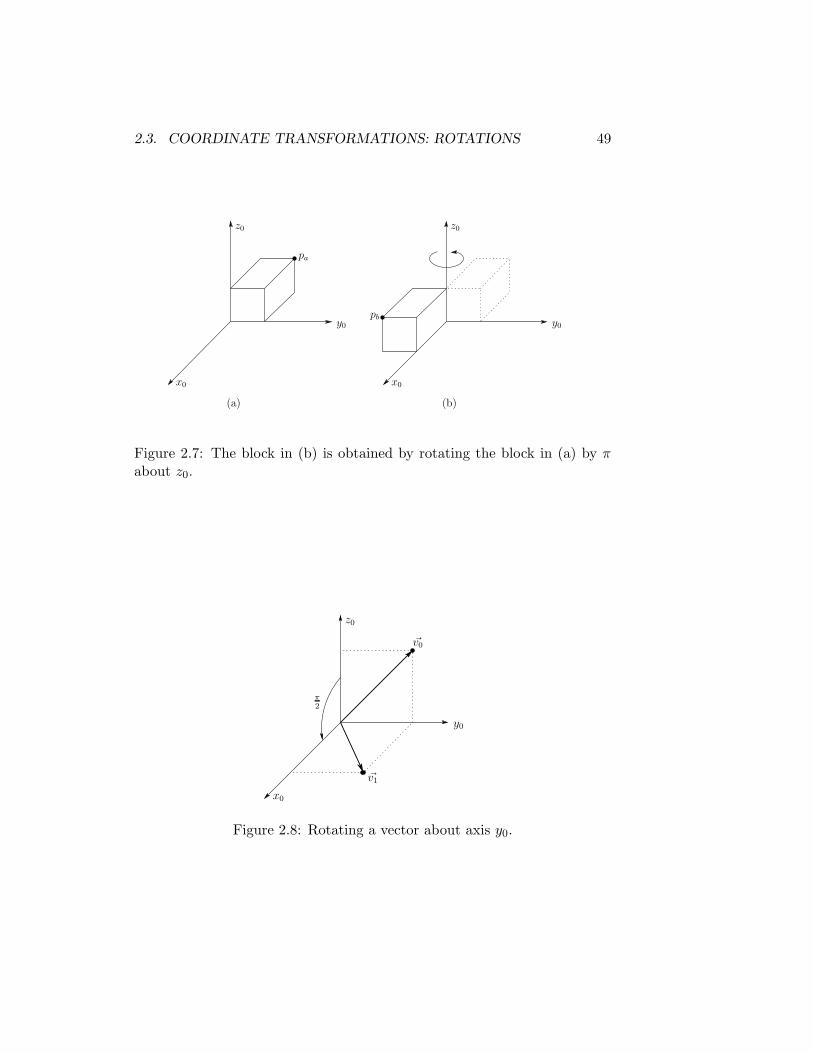
entation of one frame to another frame, and to assign coordinate represen-tations to points and vectors. For example, given a point p in space, wehave shown how a rotation matrix can be used to derive coordinates for pwith respect to different coordinate frames whose orientations are relatedby a rotation matrix. We can also use rotation matrices to represent rigidmotions that correspond to pure rotation. Consider Figure 2.7. One cornerof the block in Figure 2.7(a) is located at the point pa in space. Figure2.7(b) shows the same block after it has been rotated about z0 by the angleπ. In Figure 2.7(b), the same corner of the block is now located at point pbin space. It is possible to derive the coordinates for pb given only the coordi-nates for pa and the rotation matrix that corresponds to the rotation aboutz0. To see how this can be accomplished, imagine that a coordinate frame isrigidly attached to the block in Figure 2.7(a), such that it is coincident withthe frame o0x0y0z0. After the rotation by π, the block’s coordinate frame,which is rigidly attached to the block, is also rotated by π. If we denote thisrotated frame by o1x1y1z1, we obtain

R0

1= Rz,π =

−1 0 00 −1 00 0 1

. (2.28)


In the local coordinate frame o1x1y1z1, the point pb has the coordinaterepresentation p1

b. To obtain its coordinates with respect to frame o0x0y0z0,we merely apply the coordinate transformation equation (2.27), giving

p0

b = Rz,πp1

b. (2.29)

The key thing to notice is that the local coordinates, p1

b, of the corner ofthe block do not change as the block rotates, since they are defined in termsof the block’s own coordinate frame. Therefore, when the block’s frameis aligned with the reference frame o0x0y0z0 (i.e., before the rotation isperformed), the coordinates p1

b = p0

a, since before the rotation is performed,the point pa is coincident with the corner of the block. Therefore, we cansubstitute p0

a into the previous equation to obtain

p0

b = Rz,πp0

a. (2.30)

This equation shows us how to use a rotation matrix to represent a rotationalmotion. In particular, if the point pb is obtained by rotating the point pa asdefined by the rotation matrix R, then the coordinates of pb with respect tothe reference frame are given by

p0

b = Rp0

a. (2.31)

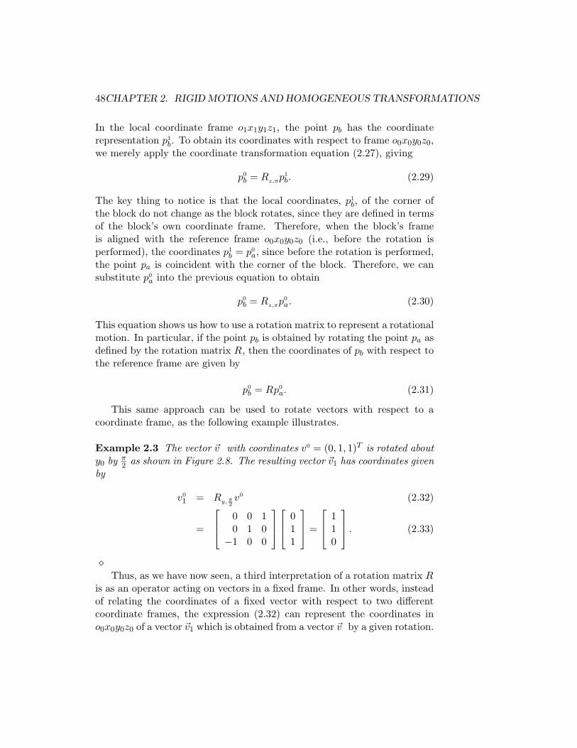
This same approach can be used to rotate vectors with respect to acoordinate frame, as the following example illustrates.

Example 2.3 The vector ~v with coordinates v0 = (0, 1, 1)T is rotated abouty0 by π

2as shown in Figure 2.8. The resulting vector ~v1 has coordinates given

by

v0

1 = Ry, π2v0 (2.32)

=

0 0 10 1 0

−1 0 0

011

=

110

. (2.33)

⋄Thus, as we have now seen, a third interpretation of a rotation matrix R

is as an operator acting on vectors in a fixed frame. In other words, insteadof relating the coordinates of a fixed vector with respect to two differentcoordinate frames, the expression (2.32) can represent the coordinates ino0x0y0z0 of a vector ~v1 which is obtained from a vector ~v by a given rotation.


z0

x0 x0

z0

pb

y0 y0

(a) (b)

pa

Figure 2.7: The block in (b) is obtained by rotating the block in (a) by π

about z0.

y0

z0

x0

�v1

�v0

π

2

Figure 2.8: Rotating a vector about axis y0.


2.3.1 Summary

We have seen that a rotation matrix, either R ∈ SO(3) or R ∈ SO(2), canbe interpreted in three distinct ways:

1. It represents a coordinate transformation relating the coordinates of apoint p in two different frames.

2. It gives the orientation of a transformed coordinate frame with respectto a fixed coordinate frame.

3. It is an operator taking a vector and rotating it to a new vector in thesame coordinate system.

The particular interpretation of a given rotation matrix R that is being usedmust then be made clear by the context.

2.4 Composition of Rotations

In this section we discuss the composition of rotations. It is important forsubsequent chapters that the reader understand the material in this sectionthoroughly before moving on.

2.4.1 Rotation with respect to the current coordinate frame

Recall that the matrix R0

1in Equation (2.27) represents a rotational trans-

formation between the frames o0x0y0z0 and o1x1y1z1. Suppose we now add athird coordinate frame o2x2y2z2 related to the frames o0x0y0z0 and o1x1y1z1by rotational transformations. As we saw above, a given point p can thenbe represented by coordinates specified with respect to any of these threeframes: p0, p1 and p2. The relationship between these representations of p is

p0 = R0

1p1 (2.34)

p1 = R1

2p2 (2.35)

p0 = R0

2p2 = R0

1R1

2p2 (2.36)

where each Rij is a rotation matrix, and equation (2.36) follows directly

by substituting equation (2.35) into equation (2.34). Note that R0

1and

R0

2represent rotations relative to the frame o0x0y0z0 while R1

2represents a

rotation relative to the frame o1x1y1z1.From equation (2.36) we can immediately infer the identity

R0

2= R0

1R1

2. (2.37)

2.4. COMPOSITION OF ROTATIONS 51

z0

x0

y0, y1x1

y2

φ

+ =

z0

x0

z1

x1

φ

y1

x2

y2

x1

y0, y1

z1, z2z1, z2

x2

θθ

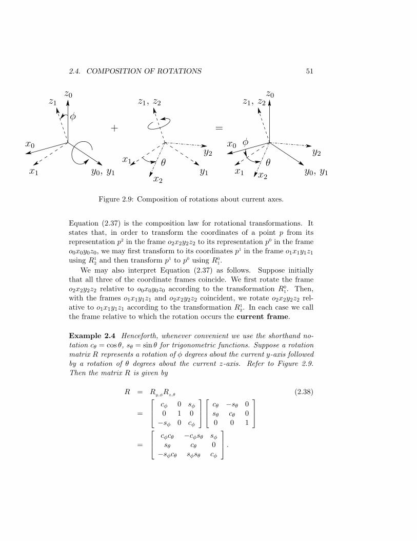
Figure 2.9: Composition of rotations about current axes.

Equation (2.37) is the composition law for rotational transformations. Itstates that, in order to transform the coordinates of a point p from itsrepresentation p2 in the frame o2x2y2z2 to its representation p0 in the frameo0x0y0z0, we may first transform to its coordinates p1 in the frame o1x1y1z1using R1

2and then transform p1 to p0 using R0

1.

We may also interpret Equation (2.37) as follows. Suppose initiallythat all three of the coordinate frames coincide. We first rotate the frameo2x2y2z2 relative to o0x0y0z0 according to the transformation R0

1. Then,

with the frames o1x1y1z1 and o2x2y2z2 coincident, we rotate o2x2y2z2 rel-ative to o1x1y1z1 according to the transformation R1

2. In each case we call

the frame relative to which the rotation occurs the current frame.

Example 2.4 Henceforth, whenever convenient we use the shorthand no-tation cθ = cos θ, sθ = sin θ for trigonometric functions. Suppose a rotationmatrix R represents a rotation of φ degrees about the current y-axis followedby a rotation of θ degrees about the current z-axis. Refer to Figure 2.9.Then the matrix R is given by

R = Ry,φRz,θ (2.38)

=

cφ 0 sφ0 1 0

−sφ 0 cφ

cθ −sθ 0sθ cθ 00 0 1

=

cφcθ −cφsθ sφsθ cθ 0

−sφcθ sφsθ cφ

.


⋄It is important to remember that the order in which a sequence of ro-

tations are carried out, and consequently the order in which the rotationmatrices are multiplied together, is crucial. The reason is that rotation,unlike position, is not a vector quantity and is therefore not subject to thelaws of vector addition, and so rotational transformations do not commutein general.

Example 2.5 Suppose that the above rotations are performed in the reverseorder, that is, first a rotation about the current z-axis followed by a rotationabout the current y-axis. Then the resulting rotation matrix is given by

R′ = Rz,θRy,φ (2.39)

=

cθ −sφ 0sθ cθ 00 0 1

cφ 0 sφ0 1 0

−sφ 0 cφ

=

cθcφ −sθ cθsφsθcφ cθ sθsφ−sφ 0 cφ

.

Comparing (2.38) and (2.39) we see that R 6= R′.⋄

2.4.2 Rotation with respect to a fixed frame

Many times it is desired to perform a sequence of rotations, each about agiven fixed coordinate frame, rather than about successive current frames.For example we may wish to perform a rotation about x0 followed by arotation about the y0 (and not y1!). We will refer to o0x0y0z0 as the fixedframe. In this case the composition law given by equation (2.37) is notvalid. It turns out that the correct composition law in this case is simplyto multiply the successive rotation matrices in the reverse order from thatgiven by (2.37). Note that the rotations themselves are not performed inreverse order. Rather they are performed about the fixed frame instead ofabout the current frame.

To see why this is so, consider the following argument. Let o0x0y0z0 bethe reference frame. Let the frame o1x1y1z1 be obtained by performing arotation with respect to the reference frame, and let this rotation be denotedby R0

1. Now let o2x2y2z2 be obtained by performing a rotation of frame

o1x1y1z1 with respect to the reference frame (not with respect to o1x1y1z1

2.4. COMPOSITION OF ROTATIONS 53

itself). We will, for the moment, denote this rotation about the fixed frameby the matrix R. Finally, let R0

2be the rotation matrix that denotes the

orientation of frame o2x2y2z2 with respect to o0x0y0z0. We know that R0

26=

R0

1R, since this equation applies for rotation about the current frame. Thus,

we now seek to determine the matrix R1

2such that R0

2= R0

1R1

2.

In order to find this matrix, we shall proceed as follows. First, we willrotate frame o1x1y1z1 to align it with the reference frame. This can be doneby postmultiplication of R0

1by its inverse. Now, since the current frame

is aligned with the reference frame, we can postmultiply by the rotationcorresponding to R (i.e., now that the fixed reference frame coincides withthe current frame, rotation about the current frame is equivalent to rotationabout the fixed reference frame). Finally, we must undo the initial rotation,which corresponds to a postmultiplication of R0

1. When we concatenate

these operations, we obtain the following:

R0

2= R0

1R1

2(2.40)

R0

2= R0

1

[

(R0

1)−1

RR0

1

]

(2.41)

R0

2= RR0

1(2.42)

This procedure is an instance of a classical technique in engineering prob-lem solving. When confronted with a difficult problem, if one can transformthe problem into an easier problem, it is often possible to transform thesolution to this easier problem into a solution to the original, more difficultproblem. In our current case, we didn’t know how to solve the problemof rotating with respect to the fixed reference frame. Therefore, we trans-formed the problem to the problem of rotating about the current frame (byusing the rotation (R0

1)−1). We then transformed the solution for this sim-

pler problem by applying the inverse of the rotation that we initially usedto simplify the problem (i.e., we postmultiplied by R0

1).

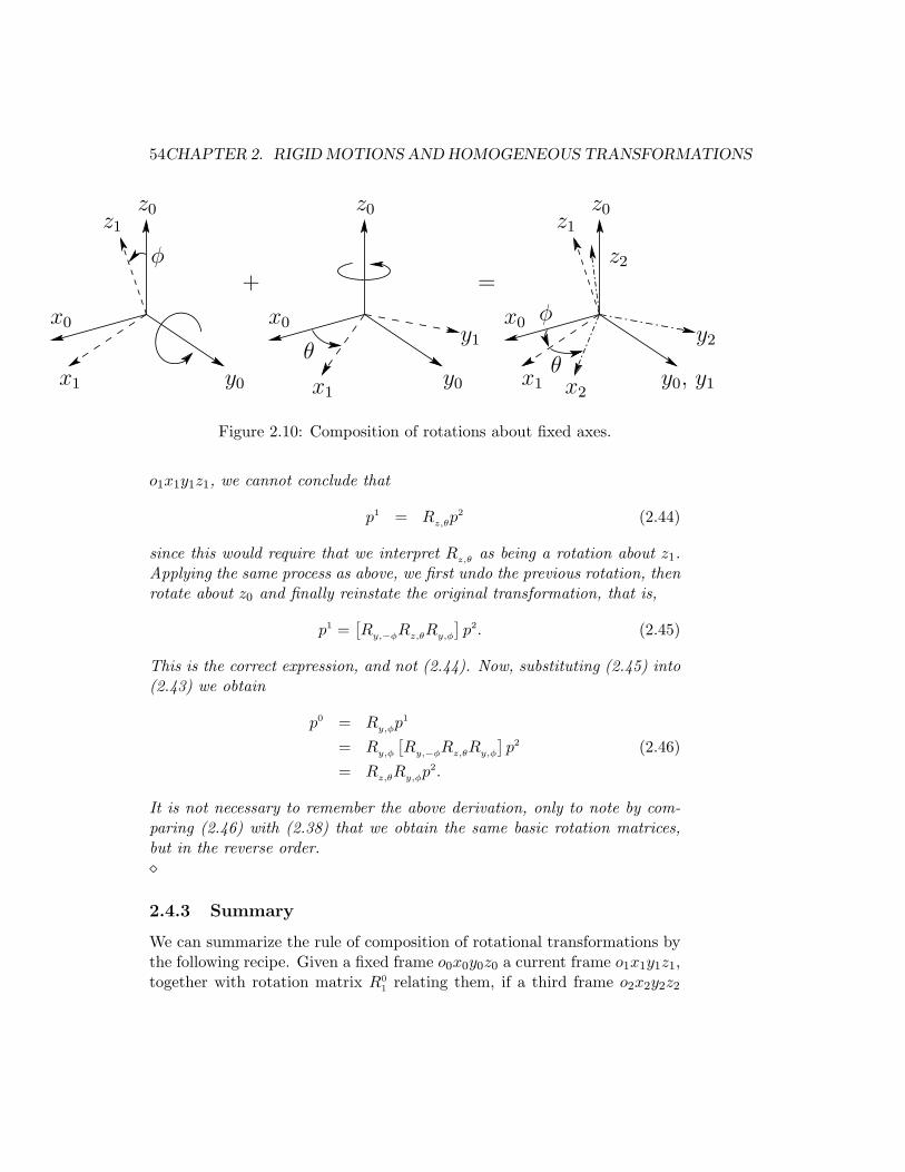
Example 2.6 Suppose that a rotation matrix R represents a rotation ofφ degrees about y0 followed by a rotation of θ about the fixed z0. Refer toFigure 2.10. Let p0, p1, and p2 be representations of a point p. Initially thefixed and current axes are the same, namely o0x0y0z0 and therefore we canwrite as before

p0 = Ry,φp1 (2.43)

where Ry,φ is the basic rotation matrix about the y-axis. Now, since thesecond rotation is about the fixed frame o0x0y0z0 and not the current frame


y0

y1

θ

z0

x0

x1

z0

x0

z0

x0

y0

z1z1

z2

x2x1

y2

x1

φ

θ

φ+ =

y0, y1

Figure 2.10: Composition of rotations about fixed axes.

o1x1y1z1, we cannot conclude that

p1 = Rz,θp2 (2.44)

since this would require that we interpret Rz,θ as being a rotation about z1.Applying the same process as above, we first undo the previous rotation, thenrotate about z0 and finally reinstate the original transformation, that is,

p1 =[

Ry,−φRz,θRy,φ

]

p2. (2.45)

This is the correct expression, and not (2.44). Now, substituting (2.45) into(2.43) we obtain

p0 = Ry,φp1

= Ry,φ

[

Ry,−φRz,θRy,φ

]

p2 (2.46)

= Rz,θRy,φp2.

It is not necessary to remember the above derivation, only to note by com-paring (2.46) with (2.38) that we obtain the same basic rotation matrices,but in the reverse order.⋄

2.4.3 Summary

We can summarize the rule of composition of rotational transformations bythe following recipe. Given a fixed frame o0x0y0z0 a current frame o1x1y1z1,together with rotation matrix R0

1relating them, if a third frame o2x2y2z2

2.5. PARAMETERIZATIONS OF ROTATIONS 55

is obtained by a rotation R performed relative to the current frame thenpostmultiply R0

1by R = R1

2to obtain

R0

2= R0

1R1

2. (2.47)

If the second rotation is to be performed relative to the fixed frame thenit is both confusing and inappropriate to use the notation R1

2to represent

this rotation. Therefore, if we represent the rotation by R, we premultiplyR0

1by R to obtain

R0

2= RR0

1. (2.48)

In each case R0

2represents the transformation between the frames o0x0y0z0

and o2x2y2z2. The frame o2x2y2z2 that results in (2.47) will be differentfrom that resulting from (2.48).

2.5 Parameterizations of Rotations

The nine elements rij in a general rotational transformation R are not inde-pendent quantities. Indeed a rigid body possesses at most three rotationaldegrees-of-freedom and thus at most three quantities are required to specifyits orientation. This can be easily seen by examining the constraints thatgovern the matrices in SO(3):

∑

i

r2ij = 1, j ∈ {1, 2, 3} (2.49)

r1ir1j + r2ir2j + r3ir3j = 0, i 6= j. (2.50)

Equation (2.49) follows from the fact the the columns of a rotation matrixare unit vectors, and (2.50) follows from the fact that columns of a rotationmatrix are mutually orthogonal. Together, these constraints define six inde-pendent equations with nine unknowns, which implies that there are threefree variables.

In this section we derive three ways in which an arbitrary rotation canbe represented using only three independent quantities: the Euler An-gle representation, the roll-pitch-yaw representation, and the axis/anglerepresentation.

2.5.1 Euler Angles

A common method of specifying a rotation matrix in terms of three inde-pendent quantities is to use the so-called Euler Angles. Consider again


ya ya, yb

x0

φ

zb

θy0

za

yb

x1

y1

ψzb, z1

xa

z0, za

xa

xb

(2)(1) (3)

xb

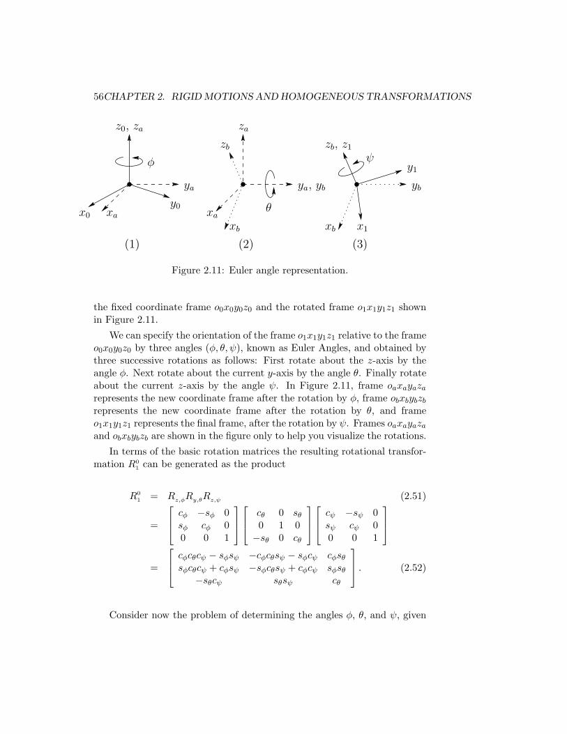
Figure 2.11: Euler angle representation.

the fixed coordinate frame o0x0y0z0 and the rotated frame o1x1y1z1 shownin Figure 2.11.

We can specify the orientation of the frame o1x1y1z1 relative to the frameo0x0y0z0 by three angles (φ, θ, ψ), known as Euler Angles, and obtained bythree successive rotations as follows: First rotate about the z-axis by theangle φ. Next rotate about the current y-axis by the angle θ. Finally rotateabout the current z-axis by the angle ψ. In Figure 2.11, frame oaxayazarepresents the new coordinate frame after the rotation by φ, frame obxbybzbrepresents the new coordinate frame after the rotation by θ, and frameo1x1y1z1 represents the final frame, after the rotation by ψ. Frames oaxayazaand obxbybzb are shown in the figure only to help you visualize the rotations.

In terms of the basic rotation matrices the resulting rotational transfor-mation R0

1can be generated as the product

R0

1= Rz,φRy,θRz,ψ (2.51)

=

cφ −sφ 0sφ cφ 00 0 1

cθ 0 sθ0 1 0

−sθ 0 cθ

cψ −sψ 0sψ cψ 00 0 1

=

cφcθcψ − sφsψ −cφcθsψ − sφcψ cφsθsφcθcψ + cφsψ −sφcθsψ + cφcψ sφsθ

−sθcψ sθsψ cθ

. (2.52)

Consider now the problem of determining the angles φ, θ, and ψ, given


the rotation matrix

R =

r11 r12 r13r21 r22 r23r31 r32 r33

. (2.53)

Suppose that not both of r13, r23 are zero. Then the above equationsshow that sθ 6= 0, and hence that not both of r31, r32 are zero. If not both

r13 and r23 are zero, then r33 6= ±1, and we have cθ = r33, sθ = ±√

1 − r233so

θ = A tan

(

r33,√

1 − r233

)

(2.54)

or

θ = A tan

(

r33,−√

1 − r233

)

. (2.55)

The function θ = A tan(x, y) computes the arc tangent function, wherex and y are the cosine and sine, respectively, of the angle θ. This functionuses the signs of x and y to select the appropriate quadrant for the angle θ.Note that if both x and y are zero, A tan is undefined.

If we choose the value for θ given by Equation (4.33), then sθ > 0, and

φ = A tan(r13, r23) (2.56)

ψ = A tan(−r31, r32). (2.57)

If we choose the value for θ given by Equation (4.34), then sθ < 0, and

φ = A tan(−r13,−r23) (2.58)

ψ = A tan(r31,−r32). (2.59)

Thus there are two solutions depending on the sign chosen for θ.If r13 = r23 = 0, then the fact that R is orthogonal implies that r33 = ±1,

and that r31 = r32 = 0. Thus R has the form

R =

r11 r12 0r21 r22 00 0 ±1.

(2.60)

If r33 = 1, then cθ = 1 and sθ = 0, so that θ = 0. In this case (2.52) becomes

cφcψ − sφsψ −cφsψ − sφcψ 0sφcψ + cφsψ −sφsψ + cφcψ 0

0 0 1

=

cφ+ψ −sφ+ψ 0sφ+ψ cφ+ψ 0

0 0 1

=

r11 r12 0r21 r22 00 0 1

(2.61)


Thus the sum φ+ ψ can be determined as

φ+ ψ = A tan(r11, r21) (2.62)

= A tan(r11,−r12).

Since only the sum φ+ψ can be determined in this case there are infinitelymany solutions. We may take φ = 0 by convention, and define ψ by (4.39).If r33 = −1, then cθ = −1 and sθ = 0, so that θ = π. In this case (2.52)becomes

−cφ−ψ −sφ−ψ 0sφ−ψ cφ−ψ 0

0 0 1

=

r11 r12 0r21 r22 00 0 −1

. (2.63)

The solution is thus

φ− ψ = A tan(−r11,−r12) = A tan(−r21,−r22). (2.64)

As before there are infinitely many solutions.

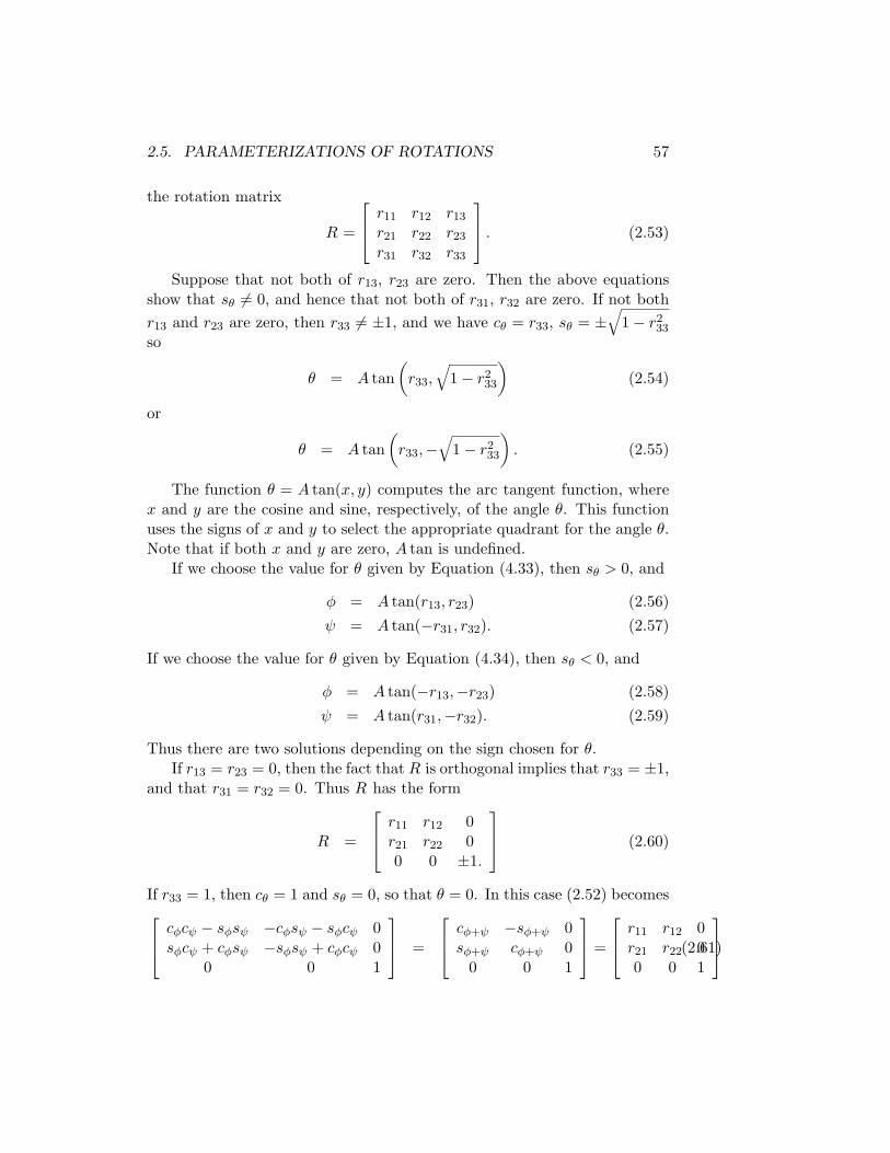
2.5.2 Roll, Pitch, Yaw Angles

A rotation matrix R can also be described as a product of successive rota-tions about the principal coordinate axes x0, y0, and z0 taken in a specificorder. These rotations define the roll, pitch, and yaw angles, which weshall also denote φ, θ, ψ, and which are shown in Figure 2.12. We specify

x0

Yaw

Roll

y0

z0

Pitch

Figure 2.12: Roll, pitch, and yaw angles.

the order of rotation as x − y − z, in other words, first a yaw about x0


through an angle ψ, then pitch about the y0 by an angle θ, and finally rollabout the z0 by an angle φ. Since the successive rotations are relative tothe fixed frame, the resulting transformation matrix is given by

R0

1= Rz,φRy,θRx,ψ (2.65)

=

cφ −sφ 0sφ cφ 00 0 1

cθ 0 sθ0 1 0

−sθ 0 cθ

1 0 00 cψ −sψ0 sψ cψ

=

cφcθ −sφcψ + cφsθsψ sφsψ + cφsθcψsφcθ cφcψ + sφsθsψ −cφsψ + sφsθcψ−sθ cθsψ cθcψ

.

Of course, instead of yaw-pitch-roll relative to the fixed frames we couldalso interpret the above transformation as roll-pitch-yaw, in that order, eachtaken with respect to the current frame. The end result is the same matrix(2.65).

The three angles, φ, θ, ψ, can be obtained for a given rotation matrixusing a method that is similar to that used to derive the Euler angles above.We leave this as an exercise for the reader.

2.5.3 Axis/Angle Representation

Rotations are not always performed about the principal coordinate axes.We are often interested in a rotation about an arbitrary axis in space. Thisprovides both a convenient way to describe rotations, and an alternativeparameterization for rotation matrices. Let k = (kx, ky, kz)

T , expressed inthe frame o0x0y0z0, be a unit vector defining an axis. We wish to derive therotation matrix R

k,θrepresenting a rotation of θ degrees about this axis.

There are several ways in which the matrix Rk,θ

can be derived. Perhaps

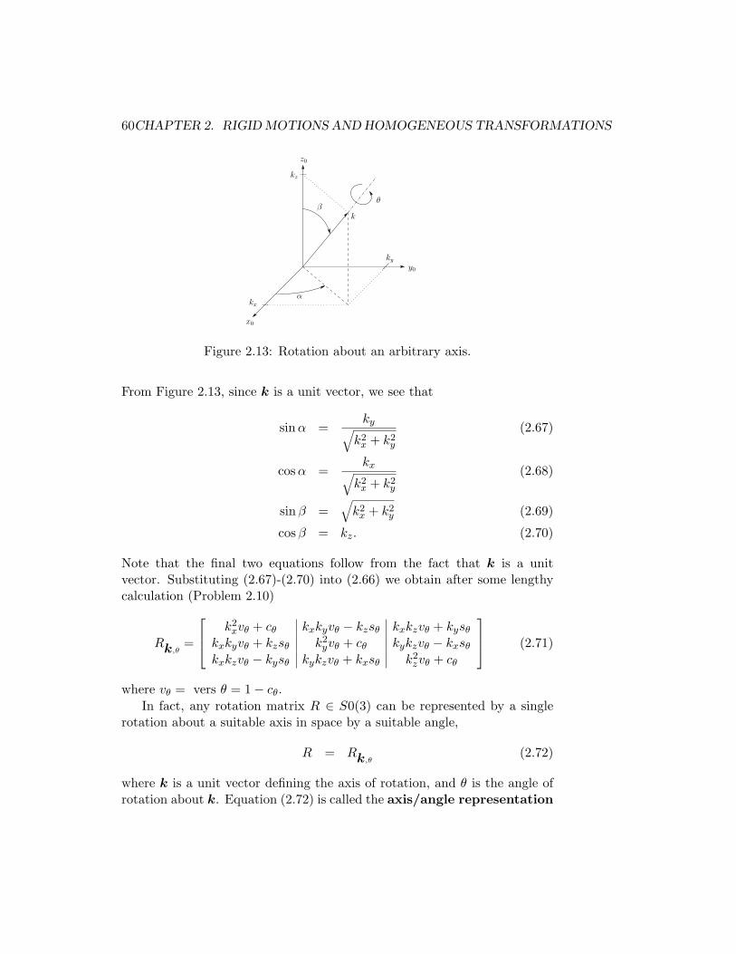
the simplest way is to rotate the vector k into one of the coordinate axes,say z0, then rotate about z0 by θ and finally rotate k back to its originalposition. This is similar to the method that we employed above to derivethe equation for rotation with respect to a fixed reference frame. Referringto Figure 2.13 we see that we can rotate k into z0 by first rotating aboutz0 by −α, then rotating about y0 by −β. Since all rotations are performedrelative to the fixed frame o0x0y0z0 the matrix R

k,θis obtained as

Rk,θ = Rz,αRy,βRz,θRy,−βRz,−α. (2.66)


βθ

x0

y0

z0

kx

ky

kz

k

α

Figure 2.13: Rotation about an arbitrary axis.

From Figure 2.13, since k is a unit vector, we see that

sinα =ky

√

k2x + k2

y

(2.67)

cosα =kx

√

k2x + k2

y

(2.68)

sinβ =√

k2x + k2

y (2.69)

cosβ = kz. (2.70)

Note that the final two equations follow from the fact that k is a unitvector. Substituting (2.67)-(2.70) into (2.66) we obtain after some lengthycalculation (Problem 2.10)

Rk,θ =

k2xvθ + cθ kxkyvθ − kzsθ kxkzvθ + kysθ

kxkyvθ + kzsθ k2yvθ + cθ kykzvθ − kxsθ

kxkzvθ − kysθ kykzvθ + kxsθ k2zvθ + cθ

(2.71)

where vθ = vers θ = 1 − cθ.

In fact, any rotation matrix R ∈ S0(3) can be represented by a singlerotation about a suitable axis in space by a suitable angle,

R = Rk,θ (2.72)

where k is a unit vector defining the axis of rotation, and θ is the angle ofrotation about k. Equation (2.72) is called the axis/angle representation


of R. Given an arbitrary rotation matrix R with components (rij), theequivalent angle θ and equivalent axis k are given by the expressions

θ = cos−1

(

Tr(R) − 1

2

)

(2.73)

= cos−1

(

r11 + r22 + r33 − 1

2

)

where Tr denotes the trace of R, and

k =1

2 sin θ

r32 − r23

r13 − r31

r21 − r12

. (2.74)

These equations can be obtained by direct manipulation of the entries ofthe matrix given in equation (2.71). The axis/angle representation is notunique since a rotation of −θ about −k is the same as a rotation of θ aboutk, that is,

Rk,θ = R−k,−θ. (2.75)

If θ = 0 then R is the identity matrix and the axis of rotation is undefined.

Example 2.7 Suppose R is generated by a rotation of 90◦ about z0 followedby a rotation of 30◦ about y0 followed by a rotation of 60◦ about x0. Then

R = Rx,60Ry,30Rz,90 (2.76)

=

0 −√

3

2

1

21

2−

√3

4−3

4√3

2

1

4

√3

4

.

We see that Tr(R) = 0 and hence the equivalent angle is given by (2.73) as

θ = cos−1

(

−1

2

)

= 120◦. (2.77)

The equivalent axis is given from (2.74) as

k =

(

1√3,

1

2√

3− 1

2,

1

2√

3+

1

2

)T

. (2.78)

⋄


θxA

xB

xC

�v1

(�v1)

(�v2)

�v2

yB

p2p1

p3

yC

�v3yA

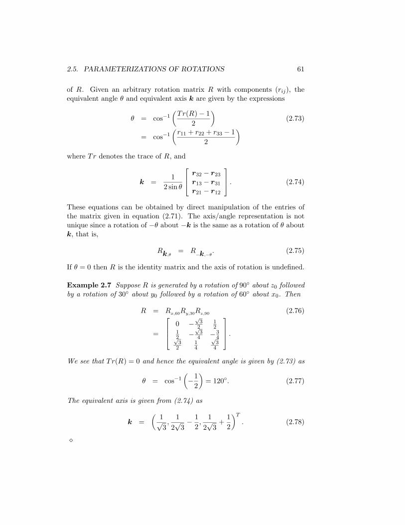
Figure 2.14: Homogeneous transformations in two dimensions.

The above axis/angle representation characterizes a given rotation byfour quantities, namely the three components of the equivalent axis k andthe equivalent angle θ. However, since the equivalent axis k is given asa unit vector only two of its components are independent. The third isconstrained by the condition that k is of unit length. Therefore, only threeindependent quantities are required in this representation of a rotation R.We can represent the equivalent angle/axis by a single vector r as

r = (rx, ry, rz)T = (θkx, θky, θkz)

T . (2.79)

Note, since k is a unit vector, that the length of the vector r is the equivalentangle θ and the direction of r is the equivalent axis k.

2.6 Homogeneous Transformations

We have seen how to represent both positions and orientations. In this sec-tion we combine these two concepts to define homogeneous transformations.

Consider Figure 2.14. In this figure, frame o1x1y1 is obtained by rotatingframe o0x0y0 by angle θ, and frame o2x2y2 is obtained by subsequentlytranslating frame o1x1y1 by the displacement ~v2. If we consider the point p1

as being rigidly attached to coordinate frame o0x0y0 as these transformationsare performed, then p2 is the location of p1 after the rotation, and p3 is thelocation of p1 after the translation. If we are given the coordinates of thepoint p3 with respect to frame o2x2y2, and if we know the rotation andtranslation that are applied to obtain frame o2x2y2, it is straightforward to

2.6. HOMOGENEOUS TRANSFORMATIONS 63

compute the coordinates of the point p3 with respect to o0x0y0. To see this,note the point p3 is displaced by the vector ~v3 from the origin of o0x0y0.Further, we see that ~v3 = ~v1 + ~v2. Therefore, to solve our problem, we needonly find coordinate assignments for the vectors ~v1 and ~v2 with respect toframe o0x0y0. Once we have these coordinate assignments, we can computethe coordinates for ~v3 with respect to o0x0y0 using the equation v0

3 = v0

1+v0

2.We can obtain coordinates for the vector ~v1 by applying the rotation

matrix to the coordinates that represent p2 in frame o1x1y1,

v0

1 = R0

1p1

2 (2.80)

= R0

2p2

3, (2.81)

where the second equality follows because the orientations of o1x1y1 ando2x2y2 are the same and because p1

2 = p2

3. If we denote the coordinateassignment for ~v2 by d0

2 (which denotes the displacement of the origin ofo2x2y2, expressed relative to o0x0y0), we obtain

p0

3 = R0

2p2

3 + d0

2. (2.82)

Note that no part of the derivation above was dependent on the fact thatwe used a two-dimensional space. This same derivation can be applied inthree dimensions to obtain the following rule for coordinate transformations.If frame o1x1y1z1 is obtained from frame o0x0y0z0 by first applying a rotationspecified by R0

1followed by a translation given (with respect to o0x0y0z0) by

d0

1, then the coordinates p0 are given by

p0 = R0

1p1 + d0

1. (2.83)

In this text, we will consider only geometric relationships between twocoordinate systems that can be expressed as the combination of a purerotation and a pure translation.

Definition 1 A transformation of the form given in Equation (2.83) is saidto define a rigid motion if R is orthogonal.

Note that the definition of a rigid motion includes reflections whendetR = −1. In our case we will never have need for the most general rigidmotion, so we assume always that R ∈ SO(3).

If we have the two rigid motions

p0 = R0

1p1 + d0

1 (2.84)


and

p1 = R1

2p2 + d1

2 (2.85)

then their composition defines a third rigid motion, which we can describeby substituting the expression for p1 from (2.85) into (2.84)

p0 = R0

1R1

2p2 +R0

1d1

2 + d0

1. (2.86)

Since the relationship between p0 and p2 is also a rigid motion, we can equallydescribe it as

p0 = R0

2p2 + d0

2. (2.87)

Comparing Equations (2.86) and (2.87) we have the relationships

R0

2= R0

1R1

2(2.88)

d0

2 = d0

1 +R0

1d1

2. (2.89)

Equation (2.88) shows that the orientation transformations can simply bemultiplied together and Equation (2.89) shows that the vector from theorigin o0 to the origin o2 has coordinates given by the sum of do1 (the vectorfrom o0 to o1 expressed with respect to o0x0y0z0) and R0

1d1

2 (the vector fromo1 to o2, expressed in the orientation of the coordinate system o0x0y0z0).

A comparison of this with the matrix identity[

R0

1d0

1

0 1

] [

R1

2d2

1

0 1

]

=

[

R0

1R1

2R0

1d2

1 + d0

1

0 1

]

(2.90)

where 0 denotes the row vector (0, 0, 0), shows that the rigid motions canbe represented by the set of matrices of the form

H =

[

R d

0 1

]

;R ∈ SO(3). (2.91)

Using the fact that R is orthogonal it is an easy exercise to show that theinverse transformation H−1 is given by

H−1 =

[

RT −RTd

0 1

]

. (2.92)

Transformation matrices of the form (2.91) are called homogeneoustransformations. In order to represent the transformation (2.83) by a

2.6. HOMOGENEOUS TRANSFORMATIONS 65

matrix multiplication, one needs to augment the vectors p0 and p1 by theaddition of a fourth component of 1 as follows. Set

P 0 =

[

p0

1

]

(2.93)

P 1 =

[

p1

1

]

. (2.94)

The vectors P 0 and P 1 are known as homogeneous representations ofthe vectors p0 and p1, respectively. It can now be seen directly that thetransformation (2.83) is equivalent to the (homogeneous) matrix equation

P 0 = H0

1P 1 (2.95)

The set of all 4 × 4 matrices H of the form (2.91) is denoted by E(3).3

A set of basic homogeneous transformations generating E(3) is givenby

Transx,a =

1 0 0 a

0 1 0 00 0 1 00 0 0 1

; Rotx,α =

1 0 0 00 cα −sα 00 sα cα 00 0 0 1

(2.96)

Transy,b =

1 0 0 00 1 0 b

0 0 1 00 0 0 1

; Roty,β =

cβ 0 sβ 00 1 0 0

−sβ 0 cβ 00 0 0 1

(2.97)

Transz,c =

1 0 0 00 1 0 00 0 1 c

0 0 0 1

; Rotx,γ =

cγ −sγ 0 0sγ cγ 0 00 0 1 00 0 0 1

(2.98)

for translation and rotation about the x, y, z-axes, respectively.The most general homogeneous transformation that we will consider may

be written now as

H0

1=

nx sx ax dxny sy ay dynz sx az dz0 0 0 1

=

[

n s a d

0 0 0 1

]

. (2.99)

3The notation E(3) stands for Euclidean group of order 3.


In the above equation n = (nx, ny, nz)T is a vector representing the direc-

tion of x1 in the o0x0y0z0 system, s = (sx, sy, sz)T represents the direc-

tion of y1, and a = (ax, ay, az)T represents the direction of z1. The vector

d = (dx, dy, dz)T represents the vector from the origin O0 to the origin O1 ex-

pressed in the frame o0x0y0z0. The rationale behind the choice of letters n, s

and a is explained in Chapter 3. NOTE: The same interpretation regarding

composition and ordering of transformations holds for 4 × 4 homogeneous

transformations as for 3 × 3 rotations.

Example 2.8 The homogeneous transformation matrix H that representsa rotation of α degrees about the current x-axis followed by a translation of bunits along the current x-axis, followed by a translation of d units along thecurrent z-axis, followed by a rotation of θ degrees about the current z-axis,is given by

H = Rotx,αTransx,bTransz,dRotz,θ (2.100)

=

1 0 0 00 cα −sα 00 sα cα 00 0 0 1

1 0 0 b

0 1 0 00 0 1 00 0 0 1

1 0 0 00 1 0 00 0 1 d

0 0 0 1

cθ −sθ 0 0sθ cθ 0 00 0 1 00 0 0 1

=

cθ −sθ 0 b

cαsα cαcθ −sα −sαdsαsθ sαcθ cα cαd

0 0 0 1

.

⋄The homogeneous representation (2.91) is a special case of homogeneous

coordinates, which have been extensively used in the field of computer graph-ics. There, one is, in addition, interested in scaling and/or perspective trans-formations. The most general homogeneous transformation takes the form

H =

[

R3×3

d3×1

f1×3 s1×1

]

=

[

Rotation Translation

perspective scale factor

]

. (2.101)

For our purposes we always take the last row vector of H to be (0, 0, 0, 1),although the more general form given by (2.101) could be useful, for example,for interfacing a vision system into the overall robotic system or for graphicsimulation.

2.7. PROBLEMS 67

2.7 Problems

1. If R is an orthogonal matrix show that the column vectors of R are ofunit length and mutually perpendicular.

2. If R is an orthogonal matrix show that detR = ±1.

3. Show that detR = ±1 if we restrict ourselves to right-handed coordi-nate systems.

4. Verify Equations (2.16)-(2.18).

5. Derive Equations (2.19) and (2.20).

6. Suppose A is a 2 × 2 rotation matrix. In other words ATA = I anddetA = 1. Show that there exists a unique θ such that A is of theform

A =

[


]

.

7. Find the rotation matrix representing a roll of π4

followed by a yaw ofπ2

followed by a pitch of π2.

8. If the coordinate frame o1x1y1z1 is obtained from the coordinate frameo0x0y0z0 by a rotation of π

2about the x-axis followed by a rotation of

π2

about the fixed y-axis, find the rotation matrix R representing thecomposite transformation. Sketch the initial and final frames.

9. Suppose that three coordinate frames o1x1y1z1, o2x2y2z2 and o3x3y3z3are given, and suppose

R1

2=

1 0 0

0 1

2−

√3

2

0√

3

2

1

2

;R1

3=

0 0 −10 1 01 0 0

.

Find the matrix R2

3.

10. Verify Equation (2.71).

11. If R is a rotation matrix show that +1 is an eigenvalue of R. Let k bea unit eigenvector corresponding to the eigenvalue +1. Give a physicalinterpretation of k.


12. Let k = 1√3(1, 1, 1)T , θ = 90◦. Find Rk,θ.

13. Show by direct calculation that Rk,θ given by (2.71) is equal to R givenby (2.76) if θ and k are given by (2.77) and (2.78), respectively.

14. Suppose R represents a rotation of 90◦ about y0 followed by a rotationof 45◦ about z1. Find the equivalent axis/angle to represent R. Sketchthe initial and final frames and the equivalent axis vector k.

15. Find the rotation matrix corresponding to the set of Euler angles{

π2, 0, π

4

}

. What is the direction of the x1 axis relative to the baseframe?

16. Compute the homogeneous transformation representing a translationof 3 units along the x-axis followed by a rotation of π

2about the current

z-axis followed by a translation of 1 unit along the fixed y-axis. Sketchthe frame. What are the coordinates of the origin O1 with respect tothe original frame in each case?

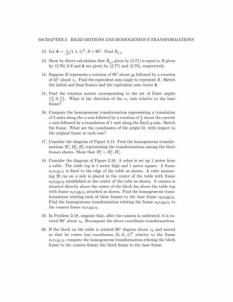
17. Consider the diagram of Figure 2.15. Find the homogeneous transfor-mations H0

1,H0

2,H1

2representing the transformations among the three

frames shown. Show that H0

2= H0

1,H1

2.

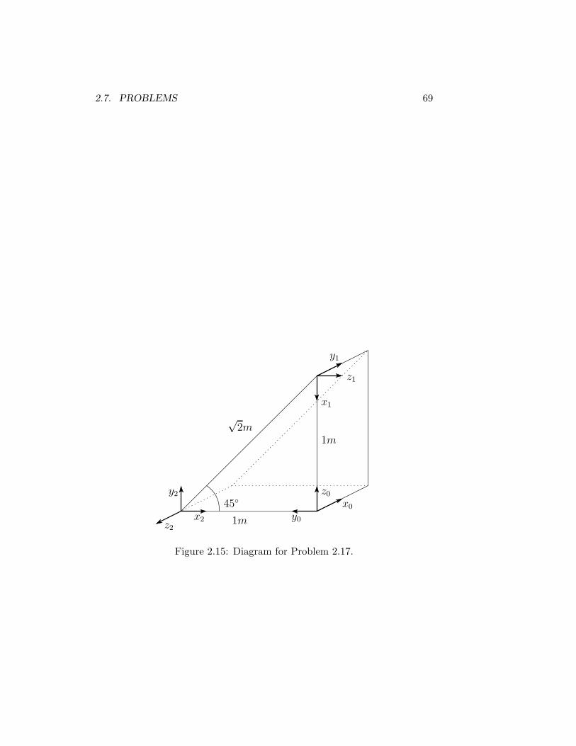
18. Consider the diagram of Figure 2.16. A robot is set up 1 meter froma table. The table top is 1 meter high and 1 meter square. A frameo1x1y1z1 is fixed to the edge of the table as shown. A cube measur-ing 20 cm on a side is placed in the center of the table with frameo2x2y2z2 established at the center of the cube as shown. A camera issituated directly above the center of the block 2m above the table topwith frame o3x3y3z3 attached as shown. Find the homogeneous trans-formations relating each of these frames to the base frame o0x0y0z0.Find the homogeneous transformation relating the frame o2x2y2z2 tothe camera frame o3x3y3z3.

19. In Problem 2-18, suppose that, after the camera is calibrated, it is ro-tated 90◦ about z3. Recompute the above coordinate transformations.

20. If the block on the table is rotated 90◦ degrees about z2 and movedso that its center has coordinates (0, .8, .1)T relative to the frameo1x1y1z1, compute the homogeneous transformation relating the blockframe to the camera frame; the block frame to the base frame.

2.7. PROBLEMS 69

1m

√

2m

1m

z0

y0x2

y2

x1

y1

z2

z1

x045◦

Figure 2.15: Diagram for Problem 2.17.


1m

1m

1m

2m

1mx0

z0

y1

x1

z1

x2

y2

z2

z3

x3y3

y0

Figure 2.16: Diagram for Problem 2.18.

Documents

Rigid Motion and Homogeneous Transformations