Embed Size (px)
Citation preview
D O C T O R A L T H E S I S | Halmstad University Dissertations No. 25
Rigorous Simulation : Its Theory and Applications
Adam Duracz

Rigorous Simulation : Its Theory and Applications© Adam DuraczHalmstad University Dissertations No. 25ISBN 978-91-87045-53-0 (printed)ISBN 978-91-87045-52-3 (pdf)Publisher: Halmstad University Press, 2016 | www.hh.se/hupPrinter: Media-Tryck, Lund


Dedicated to my parents Andrzej and Anna, and to my brother Jan.
2
Abstract 3
Abstract
Designing Cyber-Physical Systems is hard. Physical testing can beslow, expensive and dangerous. Furthermore computational compo-nents make testing all possible behavior unfeasible. Model-based de-sign mitigates these issues by making it possible to iterate over adesign much faster. Traditional simulation tools can produce usefulresults, but their results are traditionally approximations that makeit impossible to distinguish a useful simulation from one dominatedby numerical error. Verification tools require skills in formal specifi-cation and a priori understanding of the particular dynamical systembeing studied.
This thesis presents rigorous simulation, an approach to simula-tion that uses validated numerics to produce results that quantify andbound all approximation errors accumulated during simulation. Thismakes it possible for the user to objectively and reliably distinguishaccurate simulations from ones that do not provide enough informa-tion to be useful. Explicitly quantifying the error in the output hasthe side-effect of leading to a tool for dealing with inputs that comewith quantified uncertainty.
We formalize the approach as an operational semantics for a coresubset of the domain-specific language Acumen. The operational se-mantics is extended to a larger subset through a translation. Pre-liminary results toward proving the soundness of the operational se-mantics with respect to a denotational semantics are presented. Amodeling environment with a rigorous simulator based on the oper-ational semantics is described. The implementation is portable, andits source code is freely available. The accuracy of the simulator ondifferent kinds of systems is explored through a set of benchmarkmodels that exercise different aspects of a rigorous simulator. A casestudy from the automotive domain is used to evaluate the applica-bility of the simulator and its modeling language. In the case study,the simulator is used to compute rigorous bounds on the output of amodel.
4 Acknowledgments
Acknowledgments
Many people have contributed to Acumen, its theory and the ap-plications described in this thesis. The design of the language andits implementation was led by Walid Taha. Initial work on the userinterface and traditional interpreters was done by Paul Brauner. Ini-tial work on the enclosure interpreter was done by Jan Duracz. Ini-tial work on the optimized traditional interpreter was done by KevinAtkinson. The 3D visualization functionality was developed by Fei Xuand Yingfu Zeng. The current traditional and enclosure interpreters,differential equation solvers and underlying libraries were developedby myself and Ferenc A. Bartha.
The syntax and semantics (Chapters 4 and 5) are joint workwith Eugenio Moggi, Ferenc A. Bartha, and Walid Taha. EugenioMoggi contributed the denotational semantics and helped in prov-ing the soundness of the operational semantics with respect to thedenotational semantics. The case study on automotive safety (Chap-ter 7) is joint work with Ferenc A. Bartha, Ayman Aljarbouh, JawadMasood, Roland Philippsen, Henrik Eriksson, Jan Duracz, Fei Xu,Yingfu Zeng, Walid Taha, and Christian Grante. The case study onaccuracy (Chapter 8) is joint work with Ferenc A. Bartha and WalidTaha.
This work was supported by the Center for Research on Embed-ded Systems (CERES) at Halmstad University, the Swedish Knowl-edge Foundation (KK), Vinnova, and US National Science Foundationaward CPS-1136099.
On a more personal note, there are several people I want to thank,without whom I could not have finished this dissertation. My main su-pervisor Walid Taha for countless discussions and patiently remindingme to lift my gaze to see what was in front of me. My co-supervisorVeronica Gaspes for always finding the time to talk when I mostneeded it. Bertil Svensson, Roland Philippsen and Stefan Byttnerfor their support and guidance. My brother Jan for introducing meto mathematics, convincing me to pursue a PhD, and for letting mebegin this journey together with him. Ferenc A. Bartha, Amin Far-

Acknowledgments 5
judian and Michal Konecny for giving me courage to dig deeper intocomputable analysis. Eugenio Moggi for many early mornings andlate nights exploring the formal semantics of Acumen. Yingfu Zeng,Fei Xu, Kevin Atkinson, Paul Brauner and other members of theEMG for being on my team, letting me contribute to their work, andputting up with my many demands. Kevin, a special thanks for cre-ating aspell [A+2]. Saeed Gholami Shahbandi, Anita Sant’Anna andKevin LeBlanc for always being there. All my colleagues at HalmstadUniversity and climbers at HKK, for providing the fuel that kept megoing over the past five years.
Finally, I would like to thank Kazunori Ueda for agreeing to serveas opponent, and Luc Jaulin, Ian Mitchell, David Broman and JosefBigun for agreeing to serve as examiners on my defense.

6 Acknowledgments
Contents
Abstract 3
Acknowledgments 4
Notation 12
I Background 19
1 Introduction 21
1.1 Motivation . . . . . . . . . . . . . . . . . . . . . . . . 21
1.2 Thesis . . . . . . . . . . . . . . . . . . . . . . . . . . . 23
1.3 Contributions . . . . . . . . . . . . . . . . . . . . . . . 23
1.4 History and Related Publications . . . . . . . . . . . . 24
2 State of the Art 29
2.1 Modeling Formalisms . . . . . . . . . . . . . . . . . . . 29
2.2 Analysis and Tools . . . . . . . . . . . . . . . . . . . . 33
3 Traditional Simulation in Acumen 39
3.1 Past Work on Acumen . . . . . . . . . . . . . . . . . . 39
3.2 Equations . . . . . . . . . . . . . . . . . . . . . . . . . 40
3.3 Sequences of Equations . . . . . . . . . . . . . . . . . 40
3.4 If Statements . . . . . . . . . . . . . . . . . . . . . . . 41
3.5 Match Statements . . . . . . . . . . . . . . . . . . . . 42
3.6 Model Definitions and Instantiation . . . . . . . . . . 42
7
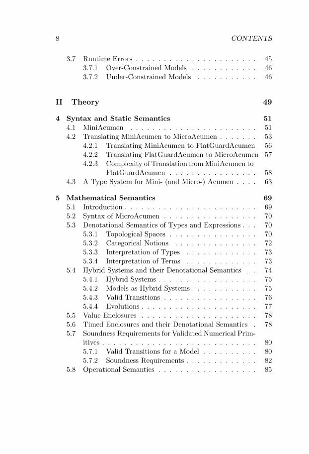
8 CONTENTS
3.7 Runtime Errors . . . . . . . . . . . . . . . . . . . . . . 45
3.7.1 Over-Constrained Models . . . . . . . . . . . . 46
3.7.2 Under-Constrained Models . . . . . . . . . . . 46
II Theory 49
4 Syntax and Static Semantics 51
4.1 MiniAcumen . . . . . . . . . . . . . . . . . . . . . . . 51
4.2 Translating MiniAcumen to MicroAcumen . . . . . . . 53
4.2.1 Translating MiniAcumen to FlatGuardAcumen 56
4.2.2 Translating FlatGuardAcumen to MicroAcumen 57
4.2.3 Complexity of Translation from MiniAcumen toFlatGuardAcumen . . . . . . . . . . . . . . . . 58
4.3 A Type System for Mini- (and Micro-) Acumen . . . . 63
5 Mathematical Semantics 69
5.1 Introduction . . . . . . . . . . . . . . . . . . . . . . . . 69
5.2 Syntax of MicroAcumen . . . . . . . . . . . . . . . . . 70
5.3 Denotational Semantics of Types and Expressions . . . 70
5.3.1 Topological Spaces . . . . . . . . . . . . . . . . 70
5.3.2 Categorical Notions . . . . . . . . . . . . . . . 72
5.3.3 Interpretation of Types . . . . . . . . . . . . . 73
5.3.4 Interpretation of Terms . . . . . . . . . . . . . 73
5.4 Hybrid Systems and their Denotational Semantics . . 74
5.4.1 Hybrid Systems . . . . . . . . . . . . . . . . . . 75
5.4.2 Models as Hybrid Systems . . . . . . . . . . . . 75
5.4.3 Valid Transitions . . . . . . . . . . . . . . . . . 76
5.4.4 Evolutions . . . . . . . . . . . . . . . . . . . . . 77
5.5 Value Enclosures . . . . . . . . . . . . . . . . . . . . . 78
5.6 Timed Enclosures and their Denotational Semantics . 78
5.7 Soundness Requirements for Validated Numerical Prim-itives . . . . . . . . . . . . . . . . . . . . . . . . . . . . 80
5.7.1 Valid Transitions for a Model . . . . . . . . . . 80
5.7.2 Soundness Requirements . . . . . . . . . . . . . 82
5.8 Operational Semantics . . . . . . . . . . . . . . . . . . 85
CONTENTS 9
5.8.1 Processing of Modes . . . . . . . . . . . . . . . 86
5.8.2 Processing of Models . . . . . . . . . . . . . . . 90
5.8.3 Example Executions . . . . . . . . . . . . . . . 91
5.9 On the Soundness of Operational Semantics . . . . . . 94
III Applications 95
6 Implementation 97
6.1 Introduction . . . . . . . . . . . . . . . . . . . . . . . . 97
6.2 Traditional and Rigorous Simulation Semantics . . . . 98
6.3 Command-Line Interface (CLI) . . . . . . . . . . . . . 99
6.4 Graphical User Interface (GUI) . . . . . . . . . . . . . 100
6.5 Organization of the Code Base . . . . . . . . . . . . . 101
6.6 Interpreters . . . . . . . . . . . . . . . . . . . . . . . . 102
6.6.1 Traditional Interpreters . . . . . . . . . . . . . 104
6.6.2 Enclosure Interpreter . . . . . . . . . . . . . . . 106
6.6.3 Active Statements . . . . . . . . . . . . . . . . 107
6.7 Artihmetics . . . . . . . . . . . . . . . . . . . . . . . . 108
6.7.1 Double . . . . . . . . . . . . . . . . . . . . . . . 108
6.7.2 Interval . . . . . . . . . . . . . . . . . . . . . . 108
6.7.3 TDif . . . . . . . . . . . . . . . . . . . . . . . . 108
6.7.4 FDif . . . . . . . . . . . . . . . . . . . . . . . . 110
6.8 Solvers . . . . . . . . . . . . . . . . . . . . . . . . . . . 110
6.8.1 Runge-Kutta . . . . . . . . . . . . . . . . . . . 110
6.8.2 Taylor . . . . . . . . . . . . . . . . . . . . . . . 111
6.8.3 Picard . . . . . . . . . . . . . . . . . . . . . . . 111
6.8.4 Lohner . . . . . . . . . . . . . . . . . . . . . . . 111
6.8.5 Contractor . . . . . . . . . . . . . . . . . . . . 112
6.8.6 Plotter and Table . . . . . . . . . . . . . . . . . 112
6.8.7 3D View . . . . . . . . . . . . . . . . . . . . . . 113
6.9 Testing . . . . . . . . . . . . . . . . . . . . . . . . . . 113
7 An Automotive Collision Case Study 115
7.1 Hazard Analysis And Risk Assessment and The ISO 26262Standard . . . . . . . . . . . . . . . . . . . . . . . . . 116
10 CONTENTS
7.2 A Collision Avoidance Scenario . . . . . . . . . . . . . 117
7.3 Vehicle and Collision Models . . . . . . . . . . . . . . 120
7.4 Vehicle Dynamics (Pre-Collision) . . . . . . . . . . . . 120
7.5 Sensing and Collision Detection . . . . . . . . . . . . . 122
7.6 Computing the Severity Class . . . . . . . . . . . . . . 123
7.7 Limitations . . . . . . . . . . . . . . . . . . . . . . . . 127
7.8 Remarks About our Experience Developing the Modelusing Acumen . . . . . . . . . . . . . . . . . . . . . . . 128
7.8.1 Avoiding Missed Events . . . . . . . . . . . . . 128
7.8.2 Avoiding Undefined Operations . . . . . . . . . 129
7.8.3 Selecting the Simulation Time Step . . . . . . . 130
8 Benchmarks for the Accuracy of Enclosures 133
8.1 Discrete and Timed Systems . . . . . . . . . . . . . . 134
8.1.1 Iteration and Nested Loops . . . . . . . . . . . 134
8.1.2 Finite Impulse Response (FIR) Filter . . . . . 140
8.2 Continuous Systems . . . . . . . . . . . . . . . . . . . 142
8.2.1 A First Order Linear System . . . . . . . . . . 142
8.2.2 A Second Order Linear System . . . . . . . . . 144
8.2.3 A Second Order Non-Linear System . . . . . . 146
8.3 Hybrid Systems . . . . . . . . . . . . . . . . . . . . . . 147
8.3.1 Discretized Sensing/Actuation . . . . . . . . . 148
8.3.2 Zeno Systems . . . . . . . . . . . . . . . . . . . 149
9 Conclusion 153
9.1 Summary of Contributions . . . . . . . . . . . . . . . . 153
9.2 Lessons Learned . . . . . . . . . . . . . . . . . . . . . 154
9.2.1 The Role of Properties in Semantics . . . . . . 155
9.2.2 Equations Versus Assignments . . . . . . . . . 155
9.2.3 Translations as a Design Tool . . . . . . . . . . 155
9.2.4 Soundness Pitfalls . . . . . . . . . . . . . . . . 156
9.3 Future Work . . . . . . . . . . . . . . . . . . . . . . . 157
9.3.1 A Richer Syntax and Semantics . . . . . . . . . 158
9.3.2 Visualization . . . . . . . . . . . . . . . . . . . 159
Appendices 161

Appendix A Preliminary Results 163
Appendix B Power Sets as Lattices 179
Bibliography 198
Glossary 199
Index 201
12 Notation
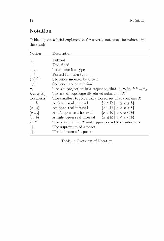
Notation
Table 1 gives a brief explanation for several notations introduced inthe thesis.
Notion Description
·↓ Defined·↑ Undefined· → · Total function type·⇀ · Partial function type〈fi〉i∈n Sequence indexed by 0 to n· ⊕ · Sequence concatenationπk· The kth projection in a sequence, that is, πk〈xi〉i∈n = xkPclosed(X) The set of topologically closed subsets of Xclosure(X) The smallest topologically closed set that contains X[a .. b] A closed real interval {x ∈ R | a ≤ x ≤ b}(a .. b) An open real interval {x ∈ R | a < x < b}(a .. b] A left-open real interval {x ∈ R | a < x ≤ b}[a .. b) A right-open real interval {x ∈ R | a ≤ x < b}T , T The lower bound T and upper bound T of interval T⊔· The supremum of a posetd· The infimum of a poset
Table 1: Overview of Notation
Notation 13
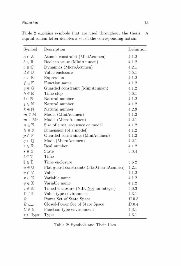
Table 2 explains symbols that are used throughout the thesis. Acapital roman letter denotes a set of the corresponding notion.
Symbol Description Definition
a ∈ A Atomic constraint (MiniAcumen) 4.1.2b ∈ B Boolean value (MiniAcumen) 4.1.2c ∈ C Dynamics (MicroAcumen) 4.2.1d ∈ D Value enclosure 5.5.1e ∈ E Expression 4.1.2f ∈ F Function name 4.1.2g ∈ G Guarded constraint (MiniAcumen) 4.1.2h ∈ R Time step 5.6.1i ∈ N Natural number 4.1.2j ∈ N Natural number 4.1.2k ∈ N Natural number 4.2.9m ∈M Model (MiniAcumen) 4.1.2m ∈Mµ Model (MicroAcumen) 4.2.1n ∈ N Size of a set, sequence or model 4.1.2N ∈ N Dimension (of a model) 4.1.2p ∈ P Guarded constraints (MiniAcumen) 4.1.2q ∈ Q Mode (MicroAcumen) 4.2.1r ∈ R Real number 4.1.2s ∈ S State 5.3.4t ∈ T Time
t ∈ T Time enclosure 5.6.2u ∈ U Flat guard constraints (FlatGuardAcumen) 4.2.1v ∈ V Value 4.1.2x ∈ X Variable name 4.1.2y ∈ X Variable name 4.1.2z ∈ Z Timed enclosure (N.B. Not an integer) 5.6.3Γ ∈ � Value type environment 4.3.1Ψ Power Set of State Space B.0.3Ψclosed Closed-Power Set of State Space B.0.4Σ ∈ � Function type environment 4.3.1τ ∈ Type Type 4.3.1
Table 2: Symbols and Their Uses

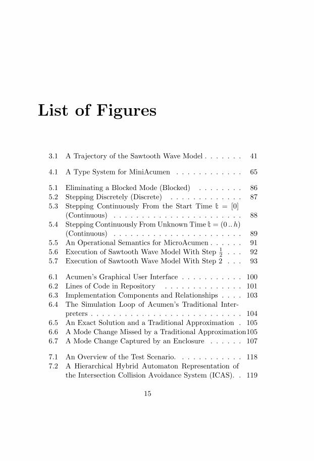
List of Figures
3.1 A Trajectory of the Sawtooth Wave Model . . . . . . . 41
4.1 A Type System for MiniAcumen . . . . . . . . . . . . 65
5.1 Eliminating a Blocked Mode (Blocked) . . . . . . . . 86
5.2 Stepping Discretely (Discrete) . . . . . . . . . . . . . 87
5.3 Stepping Continuously From the Start Time t = [0](Continuous) . . . . . . . . . . . . . . . . . . . . . . . 88
5.4 Stepping Continuously From Unknown Time t = (0 .. h)(Continuous) . . . . . . . . . . . . . . . . . . . . . . . 89
5.5 An Operational Semantics for MicroAcumen . . . . . . 91
5.6 Execution of Sawtooth Wave Model With Step 12 . . . 92
5.7 Execution of Sawtooth Wave Model With Step 2 . . . 93
6.1 Acumen’s Graphical User Interface . . . . . . . . . . . 100
6.2 Lines of Code in Repository . . . . . . . . . . . . . . 101
6.3 Implementation Components and Relationships . . . . 103
6.4 The Simulation Loop of Acumen’s Traditional Inter-preters . . . . . . . . . . . . . . . . . . . . . . . . . . . 104
6.5 An Exact Solution and a Traditional Approximation . 105
6.6 A Mode Change Missed by a Traditional Approximation105
6.7 A Mode Change Captured by an Enclosure . . . . . . 107
7.1 An Overview of the Test Scenario. . . . . . . . . . . . 118
7.2 A Hierarchical Hybrid Automaton Representation ofthe Intersection Collision Avoidance System (ICAS). . 119
15
7.3 Enclosures for Vehicle Positions and Change in Veloc-ity Due to Collision. . . . . . . . . . . . . . . . . . . . 127
7.4 Enclosures Computed With Two Different Step Sizes. 130
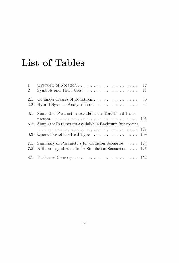
List of Tables
1 Overview of Notation . . . . . . . . . . . . . . . . . . . 122 Symbols and Their Uses . . . . . . . . . . . . . . . . . 13
2.1 Common Classes of Equations . . . . . . . . . . . . . . 302.2 Hybrid Systems Analysis Tools . . . . . . . . . . . . . 34
6.1 Simulator Parameters Available in Traditional Inter-preters. . . . . . . . . . . . . . . . . . . . . . . . . . . 106
6.2 Simulator Parameters Available in Enclosure Interpreter.. . . . . . . . . . . . . . . . . . . . . . . . . . . . . . . 107
6.3 Operations of the Real Type . . . . . . . . . . . . . . 109
7.1 Summary of Parameters for Collision Scenarios . . . . 1247.2 A Summary of Results for Simulation Scenarios. . . . 126
8.1 Enclosure Convergence . . . . . . . . . . . . . . . . . . 152
17

18 LIST OF TABLES

Part I
Background
19

Chapter 1
Introduction
“He who seeks for methods without having a definiteproblem in mind seeks in the most part in vain.”
— David Hilbert
This thesis explores a simulation approach to model-based designbased on numerical techniques that are traditionally used in verifica-tion. This chapter motivates the work, states its thesis and describesits contributions and origins.
1.1 Motivation
The miniaturization of computers has made it possible to embed oneinto practically every kind of product. These combinations, calledCyber-Physical Systems (CPS), often have completely new capabil-ities, perhaps best illustrated by the autonomy features of moderncars, or by industrial and domestic robots. As useful as these systemsare, designing them is an increasingly complex process. An importantreason for this is that the computational components of a CPS havevery large numbers of states. This makes it difficult to understandand test the behavior of the overall system. For example, it maybe too expensive or even unfeasible to perform physical tests of thesystem in each of its possible states.
21
22 CHAPTER 1. INTRODUCTION
Model-based design is one way to manage this complexity. Byperforming much of the design work on the level of a model, it becomeseasier to stage the design process to discover issues early on, whenthe cost of making mistakes is low. A model is a formal description ofthe system. If we imagine that there is an ideal or exact model, mostmodels are approximations that help the user reason about certainaspects of the system, while ignoring others. For example, a modelcan be a diagram that captures the structure of decisions made bya system or an equation that represents the positions of the physicalparts of the system.
Both diagrams and equations are examples of mathematical mod-els. Such models have the potential to be processed by computers,making simulation (observing the behavior of a model under differentconditions) easy and cheap, compared to building physical prototypes.However, even though computers have experienced an rapid gain inperformance over the past decades, many kinds of questions aboutmodels are fundamentally intractable. For example, exact solutions tomost equations cannot be computed, as doing so typically involves in-finite processes. The alternative is computing approximations, whichtypically involves truncating infinite series and using finite representa-tions of real numbers. A highly successful example is the widespreaduse of a certain class of rational numbers called “floating-point” num-bers, in place of reals. Using such numbers, many numerical methodsoriginally developed for use with reals, can be used as is, with usefulresults. Simulation tools [MAT2; Fri] based on such algorithms haveevolved to support different kinds of equational and graphical modelsthat suit the needs of different domains, and are a standard part ofan engineer’s toolkit. However, simulation tools built on conventionalnumerical methods suffer from serious and fundamental issues. Thesetools produce results that do not reflect the approximation error in-curred by the underlying numerical operations and representations.As a result, traditional simulation tools do not consistently track thiserror, and may altogether miss critical features of the model’s behav-ior. Also, the many features supported by these tools makes the taskof formally specifying their modeling languages much more difficult.
1.2. THESIS 23
Verification tools [SRKC; PQ; CAS; A+1] build on algorithmsthat are either error-free or produce results with known error bounds,and are guaranteed to take into account all behavior specified by themodel. They can analyze models with uncertain parameters, makingit possible to verify sets of scenarios simultaneously. Generally, theyare based on languages that were designed with formal semanticsin mind, and are simpler than those of simulation tools. However,there are numerous challenges en route to making verification toolsas widely used as simulation tools. These include the ability to dealwith sufficiently detailed models (scalability), to conveniently writedown the model in the given language (expressivity) and to produceinformative results (accuracy). Another challenge is the ease of useof these tools. Verification tools require the user to specify propertiesthat the tool attempts to prove. It can be particularly difficult to doso when modeling is typically done in the early stages of design, whenthe behavior of the system is not yet well understood.
1.2 Thesis
The thesis of this dissertation is that a domain-specific language forsimulation using validated numerics can combine the ease of use ofsimulation with the rigor of verification.
1.3 Contributions
The work focused on the implementation of a rigorous numerical sim-ulator for the Acumen modeling language, and makes the followingcontributions:
1. A formal specification of a flexible hybrid systems modelinglanguage (Chapter 4), which includes an operational semantics(Chapter 5) that preserves error information provided by theunderlying validated numerical methods.
2. A prototype implementation of rigorous simulation based onthis semantics, that simulates models using validated numerics.
24 CHAPTER 1. INTRODUCTION
The simulator is integrated into the freely available Acumentestbed (Chapter 6).
3. A case study of computing bounds on the output of a modelfrom the automotive domain (Chapter 7).
4. A collection of benchmarks for evaluating the accuracy of rig-orous simulators on models of stable systems (Chapter 8).
1.4 History and Related Publications
This dissertation summarizes both published and unpublished work.This section describes the origins of the chapters that are based onpublished work, and explains my contributions to the chapters thathave not been published.
My main contributions to the related publications are as follows:
1. Adam Duracz, Henrik Eriksson, Ferenc A. Bartha, Yingfu Zeng,Fei Xu, and Walid Taha. Using rigorous simulation to supportISO 26262 hazard analysis and risk assessment. In 2015 IEEE12th International Conference on Embedded Software and Sys-tems (ICESS), pages 1093–1096. IEEE, August 2015
I developed the model (initially by Walid Taha and HenrikEriksson) into the form described in this dissertation (Chap-ter 7) with help from Henrik Eriksson, Ferenc A. Bartha, Ay-man Aljarbouh and Yingfu Zeng. The necessary changes toboth the rigorous and traditional simulators that resulted fromthis case study are my work.
2. Adam Duracz, Ferenc A. Bartha, and Walid Taha. Accurate rig-orous simulation should be possible for good designs. In 2016International Workshop on Symbolic and Numerical Methodsfor Reachability Analysis (SNR), pages 1–10, April 2016
1.4. HISTORY AND RELATED PUBLICATIONS 25
I implemented the rigorous simulator needed to accurately sim-ulate the discrete and hybrid models included in the paper.The differential equation solver needed to accurately simulatethe continuous models described in the paper is joint work withFerenc A. Bartha.
3. Michal Konecny, Walid Taha, Ferenc A. Bartha, Jan Duracz,Adam Duracz, and Aaron D Ames. Enclosing the behavior ofa hybrid automaton up to and beyond a Zeno point. NonlinearAnalysis: Hybrid Systems, 20:1–20, 2016
I introduced my co-authors to related work on reachability anal-ysis, which resulted in adopting the passed-waiting-list approachto computing reachability. Through my work on the numericslibrary that underlies the prototype implementation in Acumen,the team was able to reach confidence in the correct and generalrealization of the approach.
4. Yingfu Zeng, Chad Rose, Walid Taha, Adam Duracz, KevinAtkinson, Roland Philippsen, Robert Cartwright, and MarciaO’Malley. Modeling electromechanical aspects of cyber-physicalsystems. Journal of Software Engineering for Robotics, Spe-cial Issue on Domain-Specific Languages and Models for RoboticSystems, 2016
I developed the traditional simulator that underlies the resultspresented in this paper together with Ferenc A. Bartha.
5. Ayman Aljarbouh, Yingfu Zeng, Adam Duracz, Benoıt Cail-laud, and Walid Taha. Chattering-free simulation for hybriddynamical systems. In 2016 IEEE International Conference onComputational Science and Engineering, IEEE InternationalConference on Embedded and Ubiquitous Computing, and In-ternational Symposium on Distributed Computing and Applica-tions to Business, Engineering and Science. IEEE ComputerSociety, 2016
26 CHAPTER 1. INTRODUCTION
I identified the mapping of concepts necessary to implement theapproach to simulation described in the paper.
6. Walid Taha, Adam Duracz, Yingfu Zeng, Kevin Atkinson, Fer-enc A. Bartha, Paul Brauner, Jan Duracz, Fei Xu, Robert Cart-wright, Michal Konecny, Eugenio Moggi, Jawad Masood, PererikAndreasson, Jun Inoue, Anita Sant’Anna, Roland Philippsen,Alexandre Chapoutot, Marcia O’Malley, Aaron Ames, Veron-ica Gaspes, Lise Hvatum, Shyam Mehta, Henrik Eriksson, andChristian Grante. Acumen: An open-source testbed for cyber-physical systems research. In Proceedings of EAI InternationalConference on CYber physiCaL systems, iOt and sensors Net-works (CYCLONE), 2015. EAI, 2015
I was involved in most aspects of the design of Acumen through-out the course of my PhD studies and led its implementationbetween 2014 and 2016.
7. Walid Taha, Lars-Goran Hedstrom, Fei Xu, Adam Duracz, Fer-enc A. Bartha, Yingfu Zeng, Jennifer David, and Gaurav Gun-jan. Flipping a first course on cyber-physical systems–an ex-perience report. In Workshop on Embedded and Cyber-PhysicalSystems Education (WESE 2016), Pittsburgh, PA, USA, 2016
I supported several instances of the CPS course and was respon-sible for the integration of feedback from students into Acumentool.
My contributions to the unpublished parts of this dissertation are asfollows. I designed and developed the rigorous simulator, as well asthe reference implementation of the traditional simulator (Chapter 6).The rigorous simulator builds on numerical libraries that I designedand developed together with Jan Duracz and Ferenc A. Bartha. Idefined the core languages described in this dissertation, the transla-tions between them, as well as the type system (Chapter 4). I definedthe operational semantics together with Walid Taha and Ferenc A.Bartha (Chapter 5). All proofs included in this dissertation are my
1.4. HISTORY AND RELATED PUBLICATIONS 27
work (Chapter 4 and Appendix A), though advice was provided byWalid Taha, Eugenio Moggi, Ferenc A. Bartha, Jan Duracz and AminFarjudian.
This thesis was conducted in the context of the Acumen project(Paper 6). The development of a rigorous simulator for the Acumenlanguage grew out of work on simulating Zeno hybrid automata us-ing validated numerical methods (Paper 3). The theory presented inthis thesis is based on that work. However, the present formalization(Chapters 4 and 5, and Appendix A) has not been published. Theproofs (Chapter 4 and Appendix A) have been circulated, but havenot been formally peer-reviewed for the purpose of publication. Theautomotive case study (Chapter 7) was the result of participation ina project that, among other activities, evaluated the use of rigoroussimulation for risk assessment (Paper 1). The work on benchmarkingaccuracy of enclosures (Chapter 8) was inspired by a principle sug-gested by Walid Taha, which motivated the development of a rigorousdifferential equation solver capable of simulating non-linear modelsaccurately (Paper 2).
This dissertation was also influenced by other work conducted inthe context of the Acumen project. This includes work on the model-ing of electromechanical systems (Paper 4), that served as examplesof models that the rigorous simulator should be able to process. Ageneral theme throughout has been the treatment of systems that cannot be simulated with traditional methods (Papers 3 and 5).

28 CHAPTER 1. INTRODUCTION
Chapter 2
State of the Art inModeling, Simulation, andVerification of HybridSystems
Many tools are available to designers of CPS as academic or com-mercial software, ranging from simulation tools to verification tools.This chapter reviews modeling formalisms and analyses commonlysupported by such tools.
2.1 Modeling Formalisms
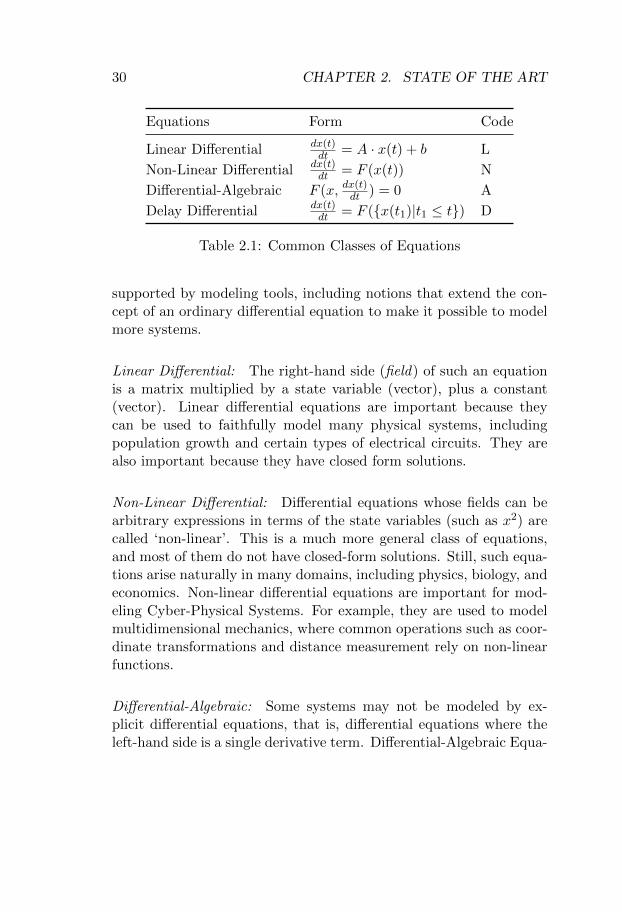
A hybrid system is a system that exhibits both discrete and con-tinuous behavior. Models of such systems describe the behavior ofvariables, and the continuous variables of a hybrid system model aretypically functions of time. Such a function can be expressed usinga differential equation. A fundamental choice in the design of a hy-brid systems modeling tool is the type of differential equations that itshould support, as this class dictates what kind of analysis that canbe supported. Table 2.1 lists common classes of differential equations
29
30 CHAPTER 2. STATE OF THE ART
Equations Form Code
Linear Differential dx(t)dt = A · x(t) + b L
Non-Linear Differential dx(t)dt = F (x(t)) N
Differential-Algebraic F (x, dx(t)dt ) = 0 A
Delay Differential dx(t)dt = F ({x(t1)|t1 ≤ t}) D
Table 2.1: Common Classes of Equations
supported by modeling tools, including notions that extend the con-cept of an ordinary differential equation to make it possible to modelmore systems.
Linear Differential: The right-hand side (field) of such an equationis a matrix multiplied by a state variable (vector), plus a constant(vector). Linear differential equations are important because theycan be used to faithfully model many physical systems, includingpopulation growth and certain types of electrical circuits. They arealso important because they have closed form solutions.
Non-Linear Differential: Differential equations whose fields can bearbitrary expressions in terms of the state variables (such as x2) arecalled ‘non-linear’. This is a much more general class of equations,and most of them do not have closed-form solutions. Still, such equa-tions arise naturally in many domains, including physics, biology, andeconomics. Non-linear differential equations are important for mod-eling Cyber-Physical Systems. For example, they are used to modelmultidimensional mechanics, where common operations such as coor-dinate transformations and distance measurement rely on non-linearfunctions.
Differential-Algebraic: Some systems may not be modeled by ex-plicit differential equations, that is, differential equations where theleft-hand side is a single derivative term. Differential-Algebraic Equa-
2.1. MODELING FORMALISMS 31
tion (DAE) are a more general class of equations, where variables andderivatives may be combined arbitrarily. A notable sub-class of suchequations are semi-explicit DAEs, whose solutions are simultaneouslyconstrained by a differential and an algebraic equation:{
dx(t)dt = F (x, y)0 = G(x, y)
DAEs provide a more modular approach to modeling. However, theycan be difficult to solve, and numerical solutions to such equationsare an active area of research [NPT].
Delay Differential: Yet another class of systems that cannot be mod-eled by ordinary differential equations are those whose behavior at agiven point in time depends not only on the current state, but alsoon past states. Examples of systems that can be modeled using a De-lay Differential Equation (DDE) are mechanical systems that exhibitvibrations and economic exchanges with information lag.
For many systems, both the discrete and continuous state of the sys-tem is of interest. In these situations, a model that combines both acontinuous dynamical model (for example, a control system’s physi-cal environment) and a discrete model (for the control system itself)is needed. Many different formalisms for hybrid systems have beenproposed, both in the scientific literature and by companies, as partof modeling environments.
Hybrid Automata: The seminal formalism for modeling hybrid sys-tems is hybrid automata [Hen], in which the behavior of continuousvariables over time is specified by constraints that include differentialequations. In a hybrid automaton, the nodes of the graph (also calleddiscrete states, modes or locations) correspond to the possible contin-uous dynamics, and the criteria for transitioning between them, calledguards, determine when the system is allowed to make a transition.Each node is also associated with an invariant . When the invariantis falsified, the system will either take a transition whose guard is
32 CHAPTER 2. STATE OF THE ART
satisfied, or it will block. Variants of hybrid automata have been ex-plored in the literature. Hybrid I/O automata [LSV] add support forparallel composition and hiding; hierarchical hybrid automata [MS]make it possible to nest automata, further facilitating the modelingof larger systems; and stochastic hybrid automata [HHHK] allow as-signing probability distributions to model parameters.
Much as with the extensions of automata described above, hybridsystems formalisms have also been developed as extensions of logic.
Hybrid Programs: Hybrid programs are textual encodings of Dif-ferential Dynamic Logic (dL) formulas [Pla1], that is, formulas ofa first-order dynamic logic extended with differential and algebraicequations/inequalities, and discrete jumps, among other things. Ex-istential quantifiers in a variant [Pla2] of dL can be used to modelthe dynamic creation of state variables, which is useful for modelingsystems where the number of variables is unknown. For example, ina model of a distributed highway collision avoidance system [LPN]that controls the vehicles on a certain part of a highway, the arrivalof vehicles into the system’s field of view corresponds to the creationof state variables.
HydLa: HydLa [UMT+] is a language based on temporal logic ex-tended with constructs for derivatives, referring to the value of avariable just before a discontinuity, and for expressing priorities be-tween constraints. The latter can be used to encode hierarchies ofconstraints. Similar to how method overriding works in class-basedobject oriented languages, this feature can be used to avoid code du-plication.
There are also formalisms that combine graphical and textual models.
Simulink: The most widely adopted industrial formalism for mod-eling of hybrid systems are the block diagrams and stateflow chartsof Simulink /Stateflow (henceforth just Simulink), both toolboxes for
2.2. ANALYSIS AND TOOLS 33
the Matlab [MAT2] scientific computing environment. First intro-duced over 20 years ago, Simulink has a large user base and thereare many libraries available for different application domains. Blockdiagrams are a graphical language in which a system is describedusing graphs, whose nodes (blocks) transform signals that can bepassed to other blocks through edges. Graph notation is convenientin domains such as electrical circuits, where the layout of the blockdiagram is close to that of the modeled system. However, systemswith many connected blocks can result in models that are difficultto read, though this issue is compensated by the ability to nest di-agrams. This language was not developed with a formally definedsemantics [CPPSV], and despite extensive work towards such a def-inition [SRKC; Tiw; ASK; MF], this work has been performed byindependent researchers, and no standard formal semantics has beenadopted.
Modelica: Another major hybrid systems formalism that has seenwide adoption is Modelica [Fri]. This is a textual language that com-bines mathematical, programmatic and graphical notations. Its keyfeatures include acausal DAEs and inheritance-based object orien-tation. In acausal equations, the left-hand side is not required tobe a single variable. Thus, models can consist of equations such asm · a = F , and the tool transforms the equation into the form (suchas a = F/m) required to solve the overall system of equations. Thisfeature helps to keep models general, as the same equation can beused in multiple contexts. Such code reuse, along with that madepossible by inheritance, helps to make it feasible to model systems ingreat detail in Modelica [SBN+].
2.2 Analysis and Tools
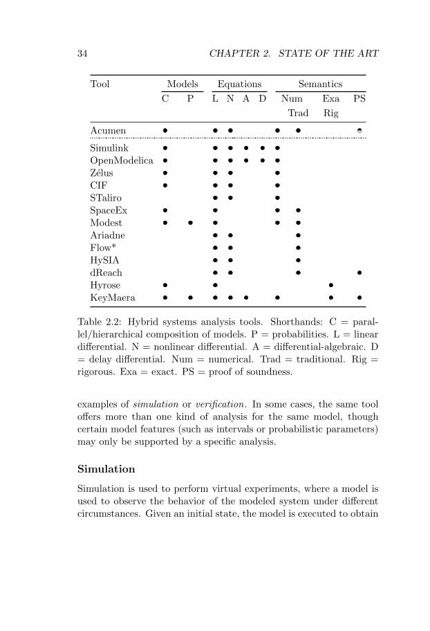
Table 2.2 lists common, actively developed hybrid systems tools. Thetools can be classified along several dimensions, including the featuressupported by their modeling formalism, as well as the types of analysisthat the tools are capable of. We may classify these analyses as
34 CHAPTER 2. STATE OF THE ART
Tool Models Equations Semantics
C P L N A D Num Exa PS
Trad Rig
Acumen
SimulinkOpenModelicaZelusCIFSTaliroSpaceExModestAriadneFlow*HySIAdReachHyroseKeyMaera
Table 2.2: Hybrid systems analysis tools. Shorthands: C = paral-lel/hierarchical composition of models. P = probabilities. L = lineardifferential. N = nonlinear differential. A = differential-algebraic. D= delay differential. Num = numerical. Trad = traditional. Rig =rigorous. Exa = exact. PS = proof of soundness.
examples of simulation or verification. In some cases, the same tooloffers more than one kind of analysis for the same model, thoughcertain model features (such as intervals or probabilistic parameters)may only be supported by a specific analysis.
Simulation
Simulation is used to perform virtual experiments, where a model isused to observe the behavior of the modeled system under differentcircumstances. Given an initial state, the model is executed to obtain
2.2. ANALYSIS AND TOOLS 35
simulation trace (trajectory). For a hybrid system model this traceconsists of piecewise solutions to differential equations, interrupted bydiscontinuities (events). A simulator for a hybrid systems modelingformalism must therefore perform two tasks. First, it must solveinitial-value problems to simulate the model’s continuous behavior.Second, it must monitor these solutions to identify when an eventshould occur (event detection), and what the behavior should be atthe discontinuity (event handling).
Equation solving generally begins with model transformation, wherethe raw model is translated into an executable form, typically consist-ing of explicit Ordinary Differential Equation (ODE) systems. Theseequations are then solved using an integrator (solver).
For a limited class of differential equations, analytic solutions canbe obtained computationally. Assuming that the model contains onlyequations whose analytic solutions can be computed, simulators basedon symbolic integrators [MU; NRS] can produce error-free trajecto-ries. Because expressions for the solutions are available, these simu-lators can be used to analyze systems with uncertain parameters, asconsidering another initial state simply amounts to evaluating theseexpressions.
In general, though, solutions to differential equations must be ap-proximated. Traditional numerical integrators are rules that, giventhe state at one or more points in time, produce an estimate at thenext point in time. The progress in time made by the integratoris called the time step. The integrator approximates the solutionusing a computationally convenient function, typically a polynomial(though there are alternatives [HT]). Modern numerical integrationlibraries [HBG+] are able to solve difficult equations such as someexamples of stiff ODEs, whose solutions are particularly sensitive tothe time step, as well as some types of DAEs. An important featureof these integrators is that they will adapt their behavior to limit theestimated approximation error, by decreasing the step or otherwiseincreasing their precision when the solution moves rapidly.
Validated numerical integrators [NJC; MB1; CAP; BM; Che; KDFT]go further and produce conservative bounds on the error as part of
36 CHAPTER 2. STATE OF THE ART
the solution. To guarantee that the bounds are conservative, theseintegrators rely on validated numerics [Tuc], numerical methods re-cast atop of interval arithmetic [War; Sun; MB2]. By propagatingthe error through the simulation, validated integrators can be usedto build rigorous (interval) simulators. A side effect of being basedon validated numerics is that validated numerical solvers operate onsets (Section 5.6) rather than on points. In principle this means that,like symbolic simulators, they can analyze models with uncertain pa-rameters (Chapter 8). Recent advances in rigorous simulation tech-niques for hybrid systems include: set representations that balancecomputational complexity against precision [FLGD+; CAS], methodsfor reducing approximation error during integration [Che] and eventhandling [GI], and parallel simulation algorithms [RG].
Verification
Verification is typically used to guarantee the correct behavior ofsafety-critical systems. To achieve this, verification tools take boththe model and a property (that is, a formally stated hypothesis aboutthe model) as input, and attempt to prove1 that the property holds.The two main approaches to verification of hybrid systems are modelchecking and theorem proving .
Model Checking and Reachability
Model checking of hybrid systems proceeds by building up an ap-proximation of the reachable states of the system, a process calledreachability . In its simplest form, the model checker observes thereachable state approximations and reports an error if any state vi-olates the property. If the model checker manages to exhaust all
1The meaning of the term “verification” varies across different communities.In engineering domains, it is frequently used as a synonym for validation. In theprogramming languages and modeling communities, it typically means somethingstronger – that the tool has generated a result with formal guarantees about itscorrectness. Exceptions to this usage exist, but for the purposes of this thesis wewill take the term to mean formal verification, and call verification approachesthat do not come with correctness guarantees testing .
2.2. ANALYSIS AND TOOLS 37
the reachable states without violating the property, it considers theproperty proven. For hybrid systems, both time and the domains ofvariables are typically modeled by real numbers, so the state spaceis generally infinite. Exhausting such a state space must thereforeinvolve observing that a fixed point is reached in the reachabilitycomputation.
Due to the accumulation of approximation error the reachabilitycomputation may not reach a fixed point, even for stable systems(Chapter 8). To remain general, bounded model checking relaxes therequirement of exhausting the state space by restricting the analysisto a finite subset of the state/solution spaces. For example, the anal-ysis may only consider a bounded time interval [Gao], or observe afinite number of discontinuities [CAS]. The reachability computationof time-bounded model checking corresponds to rigorous simulation,though model checkers may choose to traverse the state space differ-ently. A model checker may analyze its output to guide the reachabil-ity computation in an attempt to establish the property. For example,in CounterExample-Guided Abstraction and Refinement (CEGAR),one alternates proof and falsification using increasingly more preciseapproximations of the sought property [RS]. Model checking is gen-erally concerned with large uncertainties, such as proving that theproperty holds for a broad range of situations.
Theorem Proving
An alternative approach to proving properties about hybrid systemsis to view the model as a logic formula, and attempt to rewrite thisformula into one that implies the property. For example, a formulathat contains a differential equation constraint could be rewritten byreplacing the differential equation with its solution, obtained froma computer algebra system such as Mathematica [Mat1]. Theoremprovers are typically interactive, as the available rules (tactics) bywhich intermediate formulas can be re-written automatically may notsuffice to complete the derivation of the sought property. Because ofthis, using a theorem prover can be daunting as, instead of plots orother visualizations, any refinements to the model must be based on

38 CHAPTER 2. STATE OF THE ART
intermediate logical formulas.
Chapter 3
Traditional Simulation inAcumen
Acumen [TDZ+] is a Domain-Specific Language (DSL) for modelingand simulation of hybrid systems. Such systems exhibit both contin-uous and discrete behavior, and the conditions for switching betweenbehaviors that depend on the state of the system. Acumen is a smallbut expressive language, with statements that can be composed andnested to facilitate modeling of large systems. Through Acumen’snotion of objects it is possible to model systems with a dynamicallychanging number of variables.
The target of this thesis has been to develop a rigorous simulatorfor the full Acumen language. This chapter reviews past work onAcumen and describes the language to provide a sense of what itwould be like once the target is reached.
3.1 Past Work on Acumen
Acumen was originally motivated by the need for a coherent toolchainfor developing CPS [TDZ+]. The first instance of the language builton the idea of Functional Reactive Programming (FRP), where thebehavior of a system is specified by composing time-indexed func-tions [EH; WH]. The basic FRP system, used to specify discrete
39
40 CHAPTER 3. TRADITIONAL SIMULATION IN ACUMEN
changes, was extended with constructs for specifying the continuousdynamics of a system [ZWI+].
The second instance of the language, which is described in this the-sis (Chapter 6), was a ground-up redesign that, among other things,introduced the object system [BT], modeling environment [ZRT+]and rigorous simulator [DEB+; KTB+]. Throughout its development,Acumen has been used in case studies [DEB+; DBT; ZRT+] as wellas for teaching courses on CPS [TCPZ2; TCPZ1; TCPZ3; THX+].
3.2 Equations
In the physics and engineering domains, continuous evolution overtime is commonly modeled using differential equations. A simpleexample of a continuous system is a clock. We can model this systemas a single variable whose derivative with respect to time is one. InAcumen such a differential equation is expressed as follows:
x’ = 1
To model changes to the state of a system that happen instanta-neously we use a discrete equation as follows:
x+ = x + 1
This model says that the next value of x is equal to the current valueof x plus 1.
3.3 Sequences of Equations
Systems with dimension greater than one can be modeled using sys-tems of equations expressed using the composition operator “,”. Forexample, we can model a sinusoid as a system of two coupled equa-tions:
p’ = v, v’ = -p
Equivalently, this system can be expressed as a higher-order differen-tial equation p’’ = -p or vector equation (p’,v’) = (v,-p).
3.4. IF STATEMENTS 41
0 1 2
1
t
x
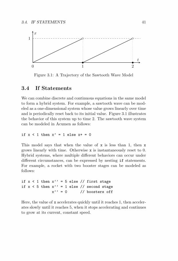
Figure 3.1: A Trajectory of the Sawtooth Wave Model
3.4 If Statements
We can combine discrete and continuous equations in the same modelto form a hybrid system. For example, a sawtooth wave can be mod-eled as a one-dimensional system whose value grows linearly over timeand is periodically reset back to its initial value. Figure 3.1 illustratesthe behavior of this system up to time 2. The sawtooth wave systemcan be modeled in Acumen as follows:
if x < 1 then x’ = 1 else x+ = 0
This model says that when the value of x is less than 1, then x
grows linearly with time. Otherwise x is instantaneously reset to 0.Hybrid systems, where multiple different behaviors can occur underdifferent circumstances, can be expressed by nesting if statements.For example, a rocket with two booster stages can be modeled asfollows:
if x < 1 then x’’ = 5 else // first stage
if x < 5 then x’’ = 1 else // second stage
x’’ = 0 // boosters off
Here, the value of x accelerates quickly until it reaches 1, then acceler-ates slowly until it reaches 5, when it stops accelerating and continuesto grow at its current, constant speed.
42 CHAPTER 3. TRADITIONAL SIMULATION IN ACUMEN
Discrete equations can be used to encode hybrid automata, that is,hybrid systems whose behavior is determined by the value of a variablewith a discrete set of values. A simple example of a hybrid automatonis a controller for a heating system:
if heating == 1
then if x < 23 then x’ = 10 else heating+ = 0
else if x > 18 then x’ = -x else heating+ = 1
Here the behavior of the system is determined by the value of theheating variable.
3.5 Match Statements
Hybrid automata can also be compactly expressed using the match
statement:
match heating with
[ 1 -> if x < 23 then x’ = 10 else heating+ = 0
| 0 -> if x > 18 then x’ = -x else heating+ = 1 ]
The different values that heating obtains during a simulation cor-respond to cases of the match, separated by “|”. We can furtherimprove the readability of this model by making heating a string-valued variable:
match heating with
[ "on" -> if x < 23 then x’ = 10 else heating+ = "off"
| "off" -> if x > 18 then x’ = -x else heating+ = "on" ]
3.6 Model Definitions and Instantiation
The examples we have seen so far are fragments of Acumen models.To be a model, such fragments must reside inside a model:
model M() = initially x = 0, x’ = 1 always x’ = 1
3.6. MODEL DEFINITIONS AND INSTANTIATION 43
A model definition consists of a name (M above), zero or more pa-rameters (zero in the model above) and two sections. The initially
section is where the initial state of the model is declared: each variablethat occurs in the model (that is not already declared as a parameter)must be specified here along with its initial value. The always sectionis where the behavior of the model is specified. The fragments thatwe have seen so far are examples of such behavior.
To be executable, an Acumen model must contain a sub-modelcalled Main with a single parameter called simulator. The simulatorparameter is used to configure the interpreter. For example, the end-time of the simulation can be changed as follows:
model Main(simulator) =
initially x = 0, x’ = 1
always x’ = 1, simulator.endTime+ = 5
Simulator parameters are modified using discrete equations. Asidefrom specifying the length of the simulation as in the model above,they can also be used to adjust the precision of the simulator, forexample by using a smaller time step. Tables 6.1 (on page 106) and6.2 (on page 107) list the simulator parameters that are available foreach type of interpreter.
Model definitions are also useful to modularize large models andto re-use code. For example, a model with two sub-models whosecontinuous behavior is described by the same differential equationcan be defined as follows:
model Trig(x,x’,x’’) = always x’’ = -x
model Main(simulator) =
initially sine = create Trig(0,1,0),
cosine = create Trig(1,0,-1)
Here, two instances (objects) of the Trig model are created by theMain model. The Main model is thus called the parent of the two Trig
objects, which in turn are called the children of the Main object. In
44 CHAPTER 3. TRADITIONAL SIMULATION IN ACUMEN
the create, the parent gives initial values to the parameters of thechild, thus possibly affecting its behavior.
Objects created in the initially section are created at the sametime as their parent. Objects can also be created dynamically byusing create in the always section, in one of two kinds of statements.First, create can occur by itself:
model Timer(p) =
initially t = 0, t’ = 1, flag = true
always t’ = 1,
if t >= 1 && flag then
create Timer(0), flag+ = false
noelse
When the t variable of a Timer object reaches 1, another Timer iscreated. The flag variable is used to ensure that each timer onlycreates a single child object. This approach can be used to createdynamic collections of objects whose size depends on the state of thesimulation.
The other way to create an object in the always section is as partof a discrete assignment. This way, a variable can be updated to referto another object during the course of a simulation:
model Timer(t,t’) = always t’ = 1
model Main(simulator) =
initially c = create Timer(0,1), flag = true
always if c.t >= 1 && flag then
c+ = create Timer(0,2), flag+ = false
noelse
Acumen’s object model allows the parent to access and modify thestate of its child objects:
model C(p) = initially t = 0, t’ = 1 always t’ = 1
3.7. RUNTIME ERRORS 45
model Main(simulator) =
initially c = create C(0)
always if c.t >= 1 then c.p+ = c.p + 1, c.t+ = 0 noelse
Here the C model has one parameter p and a variable t that trackstime. The Main object can access the values of the parameters andvariables of the C object through the name c that it was given whenit was instantiated. The Main model observes the value of c.t and,when that reaches 1, it increments the counter c.p and resets thevalue of c.t to 0.
When an object is created, it is added to the children list ofits parent. This provides another way to access the child objects, byiterating through the children list as follows:
model C(p, p’) = always p’ = p
model Main(simulator) =
initially t = 0, t’ = 1,
c1 = create C(1,1), c2 = create C(2,2)
always t’ = 1,
if t >= 1 then
t+ = 0,
foreach c in children do
( if c.className == C then c.p+ = -1/c.p noelse )
noelse
Here, the foreach statement is used to generate a set of Acumenmodel fragments, one for each child object c in the children list.This approach is useful when operating on an unbounded number ofchild objects, or when the object is not accessible through a variablename.
3.7 Runtime Errors
Several types of errors are possible in an Acumen model. In additionto syntax errors (such as mistyped keywords), or type errors (such as
46 CHAPTER 3. TRADITIONAL SIMULATION IN ACUMEN
adding a real number to a string), there are several kinds of semanticerrors:
3.7.1 Over-Constrained Models
Whenever more than one equation with a given left-hand side is activeat any step of the simulation, then the model is considered over-constrained:
model Main(simulator) =
initially x = 0, x’ = 1
always x’ = 1, if x > 1 then x’ = 2 noelse
In the model above, once x > 1 is satisfied, then both x’ = 1 andx’ = 2 are active and an error is produced.
3.7.2 Under-Constrained Models
When a discrete assignment is active, the variables that are not de-fined by any discrete assignment remain unchanged. Otherwise, eachvariable in the model must be defined by exactly one continuous equa-tion, or the model is considered under-constrained. For example, thefollowing model is under-constrained when x ≥ 1:
model Main(simulator) =
initially x = 0, x’ = 1
always if x < 1 then x’ = 1 noelse
When x is greater than 1, then no equation is active for x and anerror is generated. Thus, whenever continuous behavior is specifiedin an Acumen model, it must be given in full. Discrete behavior istreated differently. If at least one discrete equation is active, then theremaining variables are left unchanged. For example, the followingmodels are equivalent:
model Main(simulator) =
initially x = 0, x’ = 1, c = 0
3.7. RUNTIME ERRORS 47
always if x > 1 then x+ = 0, c+ = c else x’ = 1
model Main(simulator) =
initially x = 0, x’ = 1, c = 0
always if x > 1 then x+ = 0 else x’ = 1
When x > 1 in the latter model, the simulator implicitly applies theidentity discrete equation c+ = c.

48 CHAPTER 3. TRADITIONAL SIMULATION IN ACUMEN

Part II
Theory
49

Chapter 4
Syntax and StaticSemantics
This chapter formalizes the syntax for three core subsets of the Acu-men language. First, we review the syntax of MiniAcumen, a subsetof Acumen that is supported by the rigorous simulator. The seman-tics of MiniAcumen is defined by translation into a subset called Mi-croAcumen, a small subset of MiniAcumen. The translation consistsof two steps that together convert the model into a form more directlyamenable to solving by using standard numerical methods. The firststep translates MiniAcumen into a subset called FlatGuardAcumen.The bounds on the increase in the size of the term due to this trans-lation is established. Secondly, this chapter defines a simple typesystem to identify basic issues in models before simulation.
4.1 MiniAcumen
This section describes the syntax of MiniAcumen and syntactic no-tions that will be used throughout the rest of the thesis.
Definition 4.1.1 (Syntactic Notions). The syntax of MiniAcumen isdefined in terms of the following notions:
51
52 CHAPTER 4. SYNTAX AND STATIC SEMANTICS
r ∈ R Real numbersb ∈ B BooleansN ∈ N Constant natural numberx, y ∈ X Variable names, |X| = N〈xi〉i∈N Sequence of distinct variable namesf ∈ F Function names
For convenience, we identify a natural number n with the set of itspredecessors. For example, 〈xi〉i∈n becomes a proper short form for〈xi〉i∈{0...n−1}. The number N ∈ N is a constant that represents thedimension of the state space for the model being considered. �
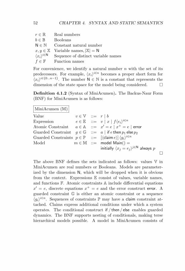
Definition 4.1.2 (Syntax of MiniAcumen). The Backus-Naur Form(BNF) for MiniAcumen is as follows:
MiniAcumen (M)
Value v ∈ V ::= r | bExpression e ∈ E ::= v | x | f〈ei〉i∈nAtomic Constraint a ∈ A ::= x′ = e | x+ = e | errorGuarded Constraint g ∈ G ::= a | if e then p1 else p2Guarded Constraints p ∈ P ::= [〈claim e〉] 〈gi〉i∈nModel m ∈M ::= model Main() =
initially 〈xj = ej〉j∈N always p�
The above BNF defines the sets indicated as follows: values V inMiniAcumen are real numbers or Booleans. Models are parameter-ized by the dimension N, which will be dropped when it is obviousfrom the context. Expressions E consist of values, variable names,and functions F. Atomic constraints A include differential equationsx′ = e, discrete equations x+ = e and the error construct error. Aguarded constraint G is either an atomic constraint or a sequence〈gi〉i∈n. Sequences of constraints P may have a claim constraint at-tached. Claims express additional conditions under which a systemoperates. The conditional construct if / then / else enables guardeddynamics. The BNF supports nesting of conditionals, making tersehierarchical models possible. A model in MiniAcumen consists of
4.2. TRANSLATION 53
an initially section, where the initial state is specified, and a set ofconstraints. We use A to denote a sequence of atoms 〈ai〉i∈n.
Notation 4.1.3 (if with empty else). We use the following short-handfor if statements with an empty else branch:
if / then if e then 〈ai〉i∈n = if e then 〈ai〉i∈n else 〈〉�
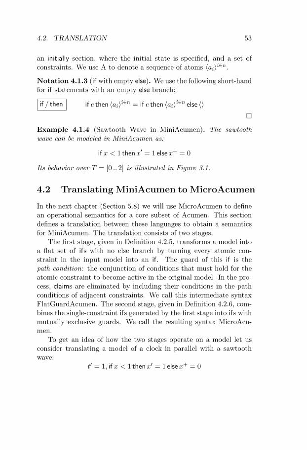
Example 4.1.4 (Sawtooth Wave in MiniAcumen). The sawtoothwave can be modeled in MiniAcumen as:
if x < 1 thenx′ = 1 elsex+ = 0
Its behavior over T = [0 .. 2] is illustrated in Figure 3.1.
4.2 Translating MiniAcumen to MicroAcumen
In the next chapter (Section 5.8) we will use MicroAcumen to definean operational semantics for a core subset of Acumen. This sectiondefines a translation between these languages to obtain a semanticsfor MiniAcumen. The translation consists of two stages.
The first stage, given in Definition 4.2.5, transforms a model intoa flat set of ifs with no else branch by turning every atomic con-straint in the input model into an if. The guard of this if is thepath condition: the conjunction of conditions that must hold for theatomic constraint to become active in the original model. In the pro-cess, claims are eliminated by including their conditions in the pathconditions of adjacent constraints. We call this intermediate syntaxFlatGuardAcumen. The second stage, given in Definition 4.2.6, com-bines the single-constraint ifs generated by the first stage into ifs withmutually exclusive guards. We call the resulting syntax MicroAcu-men.
To get an idea of how the two stages operate on a model let usconsider translating a model of a clock in parallel with a sawtoothwave:
t′ = 1, if x < 1 thenx′ = 1 elsex+ = 0
54 CHAPTER 4. SYNTAX AND STATIC SEMANTICS
The first stage produces a sequence of ifs without else branches, withone if for each atomic constraint in the original model:
〈if true then t′ = 1,〈if true ∧ x < 1 thenx′ = 1,〈if true ∧ ¬(x < 1) thenx+ = 0〉
The second stage turns the above into a sequence of mutually exclu-sive ifs:
〈 if true ∧ x > 0 ∧ ¬(x > 0) then 〈t′ = 1, x′ = 1, x+ = 0〉,if ¬true ∧ x > 0 ∧ ¬(x > 0) then 〈x′ = 1, x+ = 0〉,if true ∧ ¬(x > 0) ∧ ¬(x > 0) then 〈t′ = 1, x+ = 0〉,if ¬true ∧ ¬(x > 0) ∧ ¬(x > 0) then 〈x+ = 0〉,if true ∧ x > 0 ∧ ¬¬(x > 0) then 〈t′ = 1, x′ = 1〉,if ¬true ∧ x > 0 ∧ ¬¬(x > 0) then 〈x′ = 1〉,if true ∧ ¬(x > 0) ∧ ¬¬(x > 0) then 〈t′ = 1〉,if ¬true ∧ ¬(x > 0) ∧ ¬¬(x > 0) then 〈〉 〉
Two of these ifs have one equation per variable, that is, a completedynamics for the system:
if true ∧ ¬(x > 0) ∧ ¬(x > 0) then 〈t′ = 1, x+ = 0〉if true ∧ x > 0 ∧ ¬¬(x > 0) then 〈t′ = 1, x′ = 1〉
The remaining ifs should be considered dead code, as their guardswould always be false if they were evaluated with real numbers. How-ever, because these guards will be evaluated using set extensions ofthe normal arithmetic and Boolean operators, contradictions such asx > 0 ∧ ¬(x > 0) may evaluate to both true and false. For example,this happens when x = [−1 .. 1]. To avoid this issue, such code shouldbe eliminated during translation, or be processed by an enhancedevaluation routine that can detect such contradictions on the level ofsyntax.
The syntaxes of FlatGuardAcumen and MicroAcumen use some of thesets given in the definition of MiniAcumen (Definition 4.1.2): variablenames x ∈ X, expressions e ∈ E and atomic constraints a ∈ A.
4.2. TRANSLATION 55
Definition 4.2.1 (Syntax of FlatGuardAcumen and MicroAcumen).
FlatGuardAcumen (U)
Flat Guard Constraints u ∈ U ::= 〈if ei then 〈ai〉〉i∈n
MicroAcumen (Mµ)
Dynamics c ∈ C ::= 〈x′i = ei〉i∈N | 〈x+i = ei〉i∈N | 〈error〉Mode q ∈ Q ::= if e then cModel m ∈Mµ ::= 〈qi〉i∈n �
The above BNFs define the sets indicated as follows: flat guard con-straints U are sequences of if statements whose then branch containsa single atomic constraint, and whose else branch is empty. DynamicsC are sequences of differential equations, sequences of discrete equa-tions, or a singleton sequence containing the error construct error.Modes Q are if statements whose then branch is a dynamics, andwhose else branch is empty. MicroAcumen models Mµ are sequencesof modes.
Definition 4.2.2 (Guards, Fields and Order). We define the func-tions guard : Q → E and field : Q → En that extract the guard andfield of a mode, and the function order : M → N that extracts thedimension of a model are defined as follows:
guard(if e thenA) = efield(if e then 〈x′i = ei〉i∈N) = 〈ei〉i∈Nfield(if e then 〈x+i = ei〉i∈N) = 〈ei〉i∈Norder(model Main() = initially 〈xj = ej〉j∈N always p) = N
�
Modes are the basic building blocks of MicroAcumen. They are usedto model the dynamics 〈ai〉i∈n of a system whenever the guard con-dition e holds. We distinguish two kinds of modes: those whereai ≡ x′i = ei are called continuous modes; those where ai ≡ x+i = eiare called discrete modes.
Example 4.2.3 (Sawtooth Wave in MicroAcumen). The sawtoothwave can be modeled in MicroAcumen as:
〈if x < 1 then 〈x′ = 1〉, if x ≥ 1 then 〈x+ = 0〉〉
56 CHAPTER 4. SYNTAX AND STATIC SEMANTICS
Example 4.2.4 (Bouncing Ball in MicroAcumen). A bouncing ballwith a coefficient of restitution of 1
2 and affected by gravity with g = 10can be modeled in MicroAcumen as:
〈 if x ≤ 0 ∧ y < 0 then 〈y+ = −y2 〉
, if ¬(x ≤ 0 ∧ y < 0) then 〈x′ = y, y′ = −10〉 〉
where x and y are the vertical position and velocity of the ball respec-tively.
4.2.1 Translating MiniAcumen to FlatGuardAcumen
This section describes the first step of the translation, that is, a trans-lation from MiniAcumen to FlatGuardAcumen. In this step (Defini-tion 4.2.5), flat guard constraints are combined into mutually exclu-sive MicroAcumen modes, each of which are a complete dynamics forthe system.
The translation is based on the notion of a path condition. This isa Boolean expression, a conjunction of all the guards (Definition 4.2.2)that must be satisfied to reach the currently translated term. Thetranslation is initialized with a true path condition.
Definition 4.2.5 (Flattening Normalization). The flattening nor-malization of a constraint or set of constraints x ∈ G ∪ P at a pathcondition e ∈ E is a function ? : E× (G∪P)→Mµ defined as follows:
e ? a , 〈if e then 〈a〉〉e ? if e1 then p1 else p2 , e ∧ e1 ? p1 ⊕ e ∧ ¬e1 ? p2e ? 〈gi〉i∈n , 〈e ? gi〉i∈ne ? 〈claim ec〉 ⊕ 〈gi〉i∈n , 〈e ∧ ec ? gi〉i∈n ⊕ 〈if e ∧ ¬ec then 〈error〉〉
�
The flat normal form of the following MiniAcumen model (from M)
model Main() = initially i always p
ismodel Main() = initially i always true ? p
4.2. TRANSLATION 57
The second stage of the translation from MiniAcumen to MicroAcu-men transforms the set of modes produced by the flattening normal-ization into a set of independent modes. The modes are independentboth in the sense that their conditions are mutually exclusive, and inthat the dynamics of each mode are fully and uniquely defined.
4.2.2 Translating FlatGuardAcumen to MicroAcumen
This section describes the second step of the translation, that is, atranslation from FlatGuardAcumen to MicroAcumen. In this step(Definition 4.2.6), flat guard constraints are combined into mutuallyexclusive MicroAcumen modes, each of which are a complete dynam-ics for the system.
Definition 4.2.6 (Partitioning). The partitioning of a flat guard con-straints 〈if ei then 〈ai〉〉i∈n is the function partition : U→ Mµ definedas follows:
partition(m) =
〈〉 if m = 〈〉〈if e thenA, if ¬e then 〈〉〉 if m = 〈if e thenA〉⊕
g∈partition(m1)inject(g1, g) if m = 〈g1〉 ⊕m1
where the function inject : Q×Q→Mµ is defined as follows:
inject(if e1 then A1, if e2 then A2) =
〈if e1 ∧ e2 then A1 ⊕A2, if ¬e1 ∧ e2 then A2〉
�
Example 4.2.7 (Parallel Sub-Systems). A system with two parallel,continuous sub-systems can be modeled in FlatGuardAcumen as:
〈if e1 then 〈x′ = e2〉, if e3 then 〈y′ = e4〉〉
Its partitioned form is:
〈 if e1 ∧ e3 then 〈x′ = e2, y′ = e4〉 , if ¬e1 ∧ e3 then 〈y′ = e4〉
, if e1 ∧ ¬e3 then 〈x′ = e2〉 , if ¬e1 ∧ ¬e3 then 〈〉 〉
58 CHAPTER 4. SYNTAX AND STATIC SEMANTICS
4.2.3 Complexity of Translation from MiniAcumen toFlatGuardAcumen
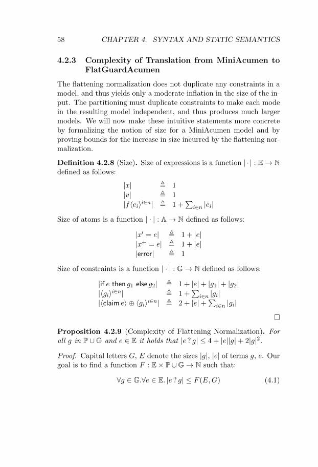
The flattening normalization does not duplicate any constraints in amodel, and thus yields only a moderate inflation in the size of the in-put. The partitioning must duplicate constraints to make each modein the resulting model independent, and thus produces much largermodels. We will now make these intuitive statements more concreteby formalizing the notion of size for a MiniAcumen model and byproving bounds for the increase in size incurred by the flattening nor-malization.
Definition 4.2.8 (Size). Size of expressions is a function | · | : E→ Ndefined as follows:
|x| , 1
|v| , 1
|f〈ei〉i∈n| , 1 +∑
i∈n |ei|
Size of atoms is a function | · | : A→ N defined as follows:
|x′ = e| , 1 + |e||x+ = e| , 1 + |e||error| , 1
Size of constraints is a function | · | : G→ N defined as follows:
|if e then g1 else g2| , 1 + |e|+ |g1|+ |g2||〈gi〉i∈n| , 1 +
∑i∈n |gi|
|〈claim e〉 ⊕ 〈gi〉i∈n| , 2 + |e|+∑
i∈n |gi|
�
Proposition 4.2.9 (Complexity of Flattening Normalization). Forall g in P ∪G and e ∈ E it holds that |e ? g| ≤ 4 + |e||g|+ 2|g|2.
Proof. Capital letters G, E denote the sizes |g|, |e| of terms g, e. Ourgoal is to find a function F : E× P ∪G→ N such that:
∀g ∈ G.∀e ∈ E. |e ? g| ≤ F (E,G) (4.1)
4.2. TRANSLATION 59
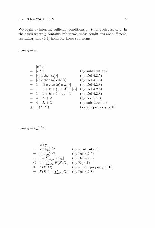
We begin by inferring sufficient conditions on F for each case of g. Inthe cases where g contains sub-terms, these conditions are sufficient,assuming that (4.1) holds for these sub-terms.
Case g ≡ a:
|e ? g|= |e ? a| (by substitution)= |〈if e then 〈a〉〉| (by Def 4.2.5)= |〈if e then 〈a〉 else 〈〉〉| (by Def 4.1.3)= 1 + |if e then 〈a〉 else 〈〉| (by Def 4.2.8)= 1 + 1 + E + (1 +A) + |〈〉| (by Def 4.2.8)= 1 + 1 + E + 1 +A+ 1 (by Def 4.2.8)= 4 + E +A (by addition)= 4 + E +G (by substitution)≤ F (E,G) (sought property of F)
Case g ≡ 〈gi〉i∈n:
|e ? g|= |e ? 〈gi〉i∈n| (by substitution)= |〈e ? gi〉i∈n| (by Def 4.2.5)= 1 +
∑i∈n |e ? gi| (by Def 4.2.8)
≤ 1 +∑
i∈n F (E,Gi) (by Eq 4.1)≤ F (E,G) (by sought property of F)= F (E, 1 +
∑i∈nGi) (by Def 4.2.8)
60 CHAPTER 4. SYNTAX AND STATIC SEMANTICS
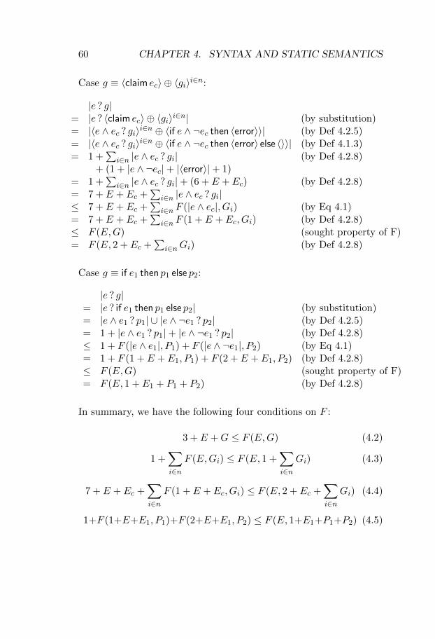
Case g ≡ 〈claim ec〉 ⊕ 〈gi〉i∈n:
|e ? g|= |e ? 〈claim ec〉 ⊕ 〈gi〉i∈n| (by substitution)= |〈e ∧ ec ? gi〉i∈n ⊕ 〈if e ∧ ¬ec then 〈error〉〉| (by Def 4.2.5)= |〈e ∧ ec ? gi〉i∈n ⊕ 〈if e ∧ ¬ec then 〈error〉 else 〈〉〉| (by Def 4.1.3)= 1 +
∑i∈n |e ∧ ec ? gi| (by Def 4.2.8)
1 + (1 + |e ∧ ¬ec|+ |〈error〉|+ 1)= 1 +
∑i∈n |e ∧ ec ? gi|+ (6 + E + Ec) (by Def 4.2.8)
= 7 + E + Ec +∑
i∈n |e ∧ ec ? gi|≤ 7 + E + Ec +
∑i∈n F (|e ∧ ec|, Gi) (by Eq 4.1)
= 7 + E + Ec +∑
i∈n F (1 + E + Ec, Gi) (by Def 4.2.8)≤ F (E,G) (sought property of F)= F (E, 2 + Ec +
∑i∈nGi) (by Def 4.2.8)
Case g ≡ if e1 then p1 else p2:
|e ? g|= |e ? if e1 then p1 else p2| (by substitution)= |e ∧ e1 ? p1| ∪ |e ∧ ¬e1 ? p2| (by Def 4.2.5)= 1 + |e ∧ e1 ? p1|+ |e ∧ ¬e1 ? p2| (by Def 4.2.8)≤ 1 + F (|e ∧ e1|, P1) + F (|e ∧ ¬e1|, P2) (by Eq 4.1)= 1 + F (1 + E + E1, P1) + F (2 + E + E1, P2) (by Def 4.2.8)≤ F (E,G) (sought property of F)= F (E, 1 + E1 + P1 + P2) (by Def 4.2.8)
In summary, we have the following four conditions on F :
3 + E +G ≤ F (E,G) (4.2)
1 +∑i∈n
F (E,Gi) ≤ F (E, 1 +∑i∈n
Gi) (4.3)
7 + E + Ec +∑i∈n
F (1 + E + Ec, Gi) ≤ F (E, 2 + Ec +∑i∈n
Gi) (4.4)
1+F (1+E+E1, P1)+F (2+E+E1, P2) ≤ F (E, 1+E1+P1+P2) (4.5)
4.2. TRANSLATION 61
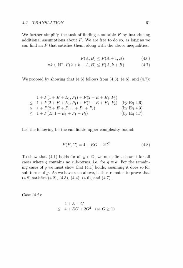
We further simplify the task of finding a suitable F by introducingadditional assumptions about F . We are free to do so, as long as wecan find an F that satisfies them, along with the above inequalities.
F (A,B) ≤ F (A+ 1, B) (4.6)
∀k ∈ N+. F (2 + k +A,B) ≤ F (A, k +B) (4.7)
We proceed by showing that (4.5) follows from (4.3), (4.6), and (4.7):
1 + F (1 + E + E1, P1) + F (2 + E + E1, P2)≤ 1 + F (2 + E + E1, P1) + F (2 + E + E1, P2) (by Eq 4.6)≤ 1 + F (2 + E + E1, 1 + P1 + P2) (by Eq 4.3)≤ 1 + F (E, 1 + E1 + P1 + P2) (by Eq 4.7)
Let the following be the candidate upper complexity bound:
F (E,G) = 4 + EG+ 2G2 (4.8)
To show that (4.1) holds for all g ∈ G, we must first show it for allcases where g contains no sub-terms, i.e. for g ≡ a. For the remain-ing cases of g we must show that (4.1) holds, assuming it does so forsub-terms of g. As we have seen above, it thus remains to prove that(4.8) satisfies (4.2), (4.3), (4.4), (4.6), and (4.7).
Case (4.2):
4 + E +G≤ 4 + EG+ 2G2 (as G ≥ 1)
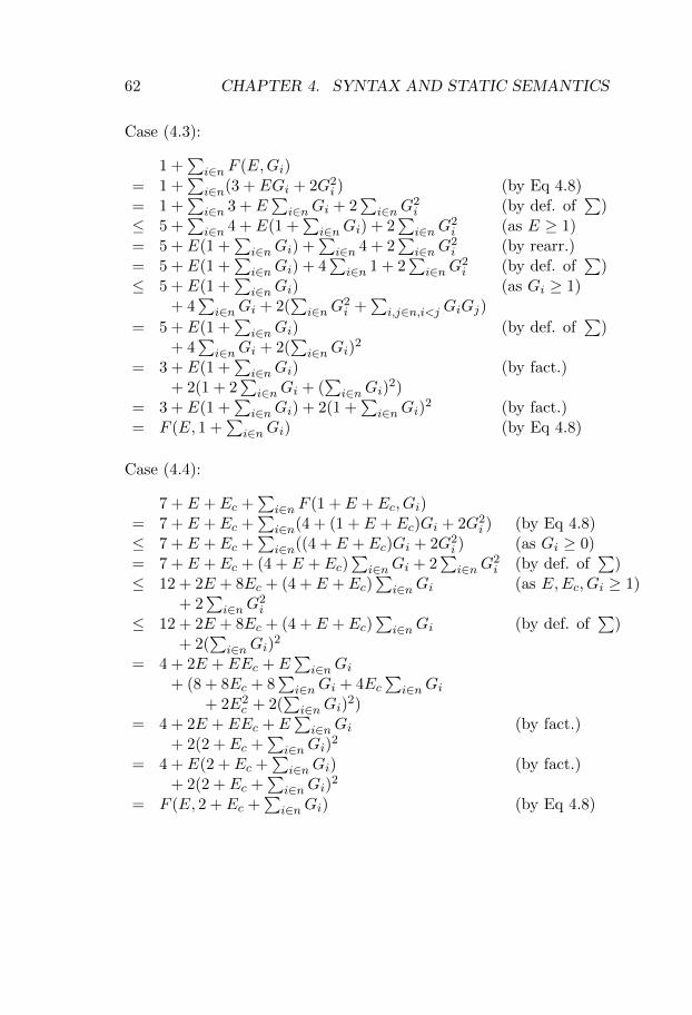
62 CHAPTER 4. SYNTAX AND STATIC SEMANTICS
Case (4.3):
1 +∑
i∈n F (E,Gi)= 1 +
∑i∈n(3 + EGi + 2G2
i ) (by Eq 4.8)= 1 +
∑i∈n 3 + E
∑i∈nGi + 2
∑i∈nG
2i (by def. of
∑)
≤ 5 +∑
i∈n 4 + E(1 +∑
i∈nGi) + 2∑
i∈nG2i (as E ≥ 1)
= 5 + E(1 +∑
i∈nGi) +∑
i∈n 4 + 2∑
i∈nG2i (by rearr.)
= 5 + E(1 +∑
i∈nGi) + 4∑
i∈n 1 + 2∑
i∈nG2i (by def. of
∑)
≤ 5 + E(1 +∑
i∈nGi) (as Gi ≥ 1)5 + 4
∑i∈nGi + 2(
∑i∈nG
2i +
∑i,j∈n,i<j GiGj)
= 5 + E(1 +∑
i∈nGi) (by def. of∑
)5 + 4
∑i∈nGi + 2(
∑i∈nGi)
2
= 3 + E(1 +∑
i∈nGi) (by fact.)3 + 2(1 + 2
∑i∈nGi + (
∑i∈nGi)
2)= 3 + E(1 +
∑i∈nGi) + 2(1 +
∑i∈nGi)
2 (by fact.)= F (E, 1 +
∑i∈nGi) (by Eq 4.8)
Case (4.4):
7 + E + Ec +∑
i∈n F (1 + E + Ec, Gi)= 7 + E + Ec +
∑i∈n(4 + (1 + E + Ec)Gi + 2G2
i ) (by Eq 4.8)≤ 7 + E + Ec +
∑i∈n((4 + E + Ec)Gi + 2G2
i ) (as Gi ≥ 0)= 7 + E + Ec + (4 + E + Ec)
∑i∈nGi + 2
∑i∈nG
2i (by def. of
∑)
≤ 12 + 2E + 8Ec + (4 + E + Ec)∑
i∈nGi (as E,Ec, Gi ≥ 1)12 + 2
∑i∈nG
2i
≤ 12 + 2E + 8Ec + (4 + E + Ec)∑
i∈nGi (by def. of∑
)12 + 2(
∑i∈nGi)
2
= 4 + 2E + EEc + E∑
i∈nGi4 + (8 + 8Ec + 8
∑i∈nGi + 4Ec
∑i∈nGi
4 + (8 + 2E2c + 2(
∑i∈nGi)
2)= 4 + 2E + EEc + E
∑i∈nGi (by fact.)
4 + 2(2 + Ec +∑
i∈nGi)2
= 4 + E(2 + Ec +∑
i∈nGi) (by fact.)4 + 2(2 + Ec +
∑i∈nGi)
2
= F (E, 2 + Ec +∑
i∈nGi) (by Eq 4.8)
4.3. A TYPE SYSTEM FOR MINI- (AND MICRO-) ACUMEN 63
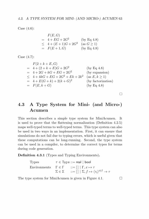
Case (4.6):
F (E,G)= 4 + EG+ 2G2 (by Eq 4.8)≤ 4 + (E + 1)G+ 2G2 (as G ≥ 1)= F (E + 1, G) (by Eq 4.8)
Case (4.7):
F (2 + k + E,G)= 4 + (2 + k + E)G+ 2G2 (by Eq 4.8)= 4 + 2G+ kG+ EG+ 2G2 (by expansion)≤ 4 + 4kG+ EG+ 2G2 + Ek + 2k2 (as E, k ≥ 1)= 4 + E(G+ k) + 2(k +G)2 (by factorization)= F (E, k +G) (by Eq 4.8)
4.3 A Type System for Mini- (and Micro-)Acumen
This section describes a simple type system for MiniAcumen. Itis used to prove that the flattening normalization (Definition 4.2.5)maps well-typed terms to well-typed terms. This type system can alsobe used in two ways in an implementation. First, it can ensure thatsimulations do not fail due to typing errors, which is useful given thatthese computations can be long-running. Second, the type systemcan be used in a compiler, to determine the correct types for termsduring code generation.
Definition 4.3.1 (Types and Typing Environments).
Types τ ∈ Type ::= real | boolEnvironments Γ ∈ � ::= [ ] | Γ, x 7→ τ
Σ ∈ � ::= [ ] | Σ, f 7→ 〈τi〉i∈I → τ
The type system for MiniAcumen is given in Figure 4.1. �
64 CHAPTER 4. SYNTAX AND STATIC SEMANTICS
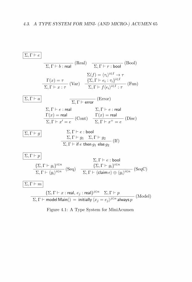
The above BNF defines the sets indicated as follows: types Type arereal or bool. Variable type environments � are empty or a variabletype environment extended with a mapping from variable name totype. Function type environments � are empty or a function type en-vironment extended with a mapping from function name to a functionfrom a list of parameter types to a result type.
The rules in Figure 4.1 define the typing relation. The Real, Bool,Var and Fun rules are used to check expressions. The Real and Boolrules establish that values are well-typed. By the Var rule a variable iswell-typed if the variable typing environment Γ contains a correspond-ing mapping. By the Fun rule a function application is well-typed ifthe function typing environment contains a corresponding mapping,and if the parameter types of that mapping match the types of theexpressions used in the application.
The Error, Cont and Disc rules are used to check atomic con-straints. The Error rule establishes that the error constraint is well-typed. By the Cont and Disc rules respectively, continuous and dis-crete equations are well-typed if the variable typing environment mapsthe left-hand side to the real, and the type of the right-hand side ex-pression is real.
By the If rule an if / then / else statement is well-typed if its condi-tion is of type bool, and if both its branches are well-typed. The Seqand SeqC rules are used to check sequences of statements. Both rulesrequire that each of the guarded constraints in the sequence is well-typed. The SeqC rule additionally requires that the claim expressionis of bool type.
By the Model rule a model is well-typed if, for each of its initial-izations, both the right and the left-hand side are of type real, and ifthe guarded constraint p is well-typed.
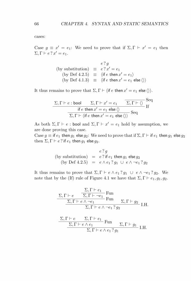
Proposition 4.3.2 (Flattening Preserves Typability). Whenever Σ ∈�,Γ ∈ �, e ∈ E, g ∈ G, and we have that Σ,Γ ` e : bool ∧ Σ,Γ ` g, pthen Σ,Γ ` e ? g, e ? p.
Proof. We proceed by induction on the structure of g. For all cases,assume that Σ,Γ ` e : bool. In what follows we consider all possible
4.3. A TYPE SYSTEM FOR MINI- (AND MICRO-) ACUMEN 65
Σ,Γ ` e
Σ,Γ ` b : real(Real)
Σ,Γ ` r : bool(Bool)
Γ(x) = τ
Σ,Γ ` x : τ(Var)
Σ(f) = 〈τi〉i∈I → τ{Σ,Γ ` ei : τi}i∈I
Σ,Γ ` f〈ei〉i∈I : τ(Fun)
Σ,Γ ` aΣ,Γ ` error
(Error)
Σ,Γ ` e : realΓ(x) = real
Σ,Γ ` x′ = e(Cont)
Σ,Γ ` e : realΓ(x) = real
Σ,Γ ` x+ = e(Disc)
Σ,Γ ` g Σ,Γ ` e : boolΣ,Γ ` g1 Σ,Γ ` g2
Σ,Γ ` if e then g1 else g2(If)
Σ,Γ ` p
{Σ,Γ ` gi}i∈n
Σ,Γ ` 〈gi〉i∈n(Seq)
Σ,Γ ` e : bool{Σ,Γ ` gi}i∈n
Σ,Γ ` 〈claim e〉 ⊕ 〈gi〉i∈n(SeqC)
Σ,Γ ` m
{Σ,Γ ` x : real, ej : real}j∈n Σ,Γ ` pΣ,Γ ` modelMain() = initially 〈xj = ej〉j∈n always p
(Model)
Figure 4.1: A Type System for MiniAcumen
66 CHAPTER 4. SYNTAX AND STATIC SEMANTICS
cases:
Case g ≡ x′ = e1: We need to prove that if Σ,Γ ` x′ = e1 thenΣ,Γ ` e ?x′ = e1.
e ? g(by substitution) ≡ e ?x′ = e1
(by Def 4.2.5) ≡ 〈if e thenx′ = e1〉(by Def 4.1.3) ≡ 〈if e thenx′ = e1 else 〈〉〉
It thus remains to prove that Σ,Γ ` 〈if e thenx′ = e1 else 〈〉〉.
Σ,Γ ` e : bool Σ,Γ ` x′ = e1Seq
Σ,Γ ` 〈〉If
if e thenx′ = e1 else 〈〉Seq
Σ,Γ ` 〈if e thenx′ = e1 else 〈〉〉
As both Σ,Γ ` e : bool and Σ,Γ ` x′ = e1 hold by assumption, weare done proving this case.
Case g ≡ if e1 then g1 else g2: We need to prove that if Σ,Γ ` if e1 then g1 else g2then Σ,Γ ` e ? if e1 then g1 else g2.
e ? g(by substitution) = e ? if e1 then g1 else g2
(by Def 4.2.5) = e ∧ e1 ? g1 ∪ e ∧ ¬e1 ? g2
It thus remains to prove that Σ,Γ ` e ∧ e1 ? g1 ∪ e ∧ ¬e1 ? g2. Wenote that by the (If) rule of Figure 4.1 we have that Σ,Γ ` e1, g1, g2.
Σ,Γ ` eΣ,Γ ` e1
FunΣ,Γ ` ¬e1
FunΣ,Γ ` e ∧ ¬e1 Σ,Γ ` g2
I.H.Σ,Γ ` e ∧ ¬e1 ? g2
Σ,Γ ` e Σ,Γ ` e1Fun
Σ,Γ ` e ∧ e1 Σ,Γ ` g1I.H.
Σ,Γ ` e ∧ e1 ? g1
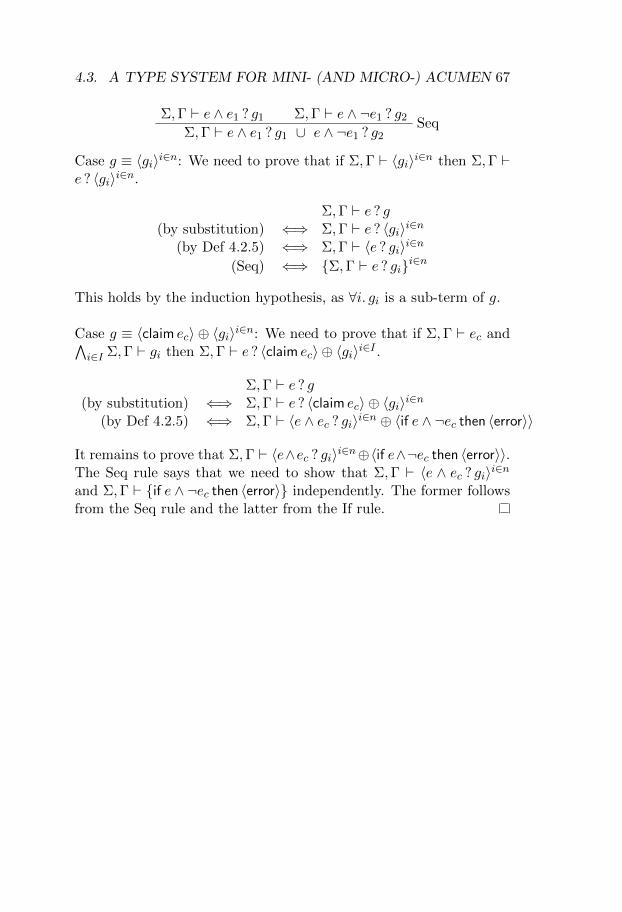
4.3. A TYPE SYSTEM FOR MINI- (AND MICRO-) ACUMEN 67
Σ,Γ ` e ∧ e1 ? g1 Σ,Γ ` e ∧ ¬e1 ? g2 SeqΣ,Γ ` e ∧ e1 ? g1 ∪ e ∧ ¬e1 ? g2
Case g ≡ 〈gi〉i∈n: We need to prove that if Σ,Γ ` 〈gi〉i∈n then Σ,Γ `e ? 〈gi〉i∈n.
Σ,Γ ` e ? g(by substitution) ⇐⇒ Σ,Γ ` e ? 〈gi〉i∈n
(by Def 4.2.5) ⇐⇒ Σ,Γ ` 〈e ? gi〉i∈n(Seq) ⇐⇒ {Σ,Γ ` e ? gi}i∈n
This holds by the induction hypothesis, as ∀i. gi is a sub-term of g.
Case g ≡ 〈claim ec〉 ⊕ 〈gi〉i∈n: We need to prove that if Σ,Γ ` ec and∧i∈I Σ,Γ ` gi then Σ,Γ ` e ? 〈claim ec〉 ⊕ 〈gi〉i∈I .
Σ,Γ ` e ? g(by substitution) ⇐⇒ Σ,Γ ` e ? 〈claim ec〉 ⊕ 〈gi〉i∈n
(by Def 4.2.5) ⇐⇒ Σ,Γ ` 〈e ∧ ec ? gi〉i∈n ⊕ 〈if e ∧ ¬ec then 〈error〉〉
It remains to prove that Σ,Γ ` 〈e∧ec ? gi〉i∈n⊕〈if e∧¬ec then 〈error〉〉.The Seq rule says that we need to show that Σ,Γ ` 〈e ∧ ec ? gi〉i∈nand Σ,Γ ` {if e ∧ ¬ec then 〈error〉} independently. The former followsfrom the Seq rule and the latter from the If rule.

68 CHAPTER 4. SYNTAX AND STATIC SEMANTICS
Chapter 5
Mathematical Semantics
This chapter defines the denotational semantics (Subsection 5.4.4)and operational semantics (Section 5.8) of MicroAcumen. The deno-tational semantics gives a meaning to MicroAcumen terms as math-ematical objects. Its purpose is to serve as an independent, unam-biguous definition against which another definition can be compared.The operational semantics is a model of the way in which the rigoroussimulator constructs enclosures. We also present a conjecture aboutthe soundness of the operational semantics with respect to the deno-tational semantics (Section 5.9). Results that may help in provingthis conjecture are given in Appendix A.
5.1 Introduction
A mathematical semantics gives meaning to the terms of a languagein a way that makes it possible to analyze the interpretation.
The following diagram illustrates the semantic functions (H(·),· ↪−→ · and [[·]]) presented in this chapter, as well as the soundnessproperty conjectured in Section 5.9.
69
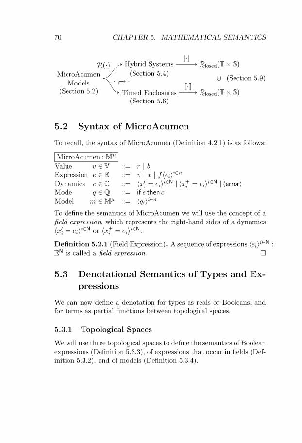
70 CHAPTER 5. MATHEMATICAL SEMANTICS
MicroAcumenModels
Hybrid Systems Pclosed(T× S)
Timed Enclosures Pclosed(T× S)
H(·)
· ↪−→ ·
[[·]]
[[·]]
⊆
(Section 5.2)
(Section 5.4)
(Section 5.6)
(Section 5.9)
5.2 Syntax of MicroAcumen
To recall, the syntax of MicroAcumen (Definition 4.2.1) is as follows:
MicroAcumen : Mµ
Value v ∈ V ::= r | bExpression e ∈ E ::= v | x | f〈ei〉i∈nDynamics c ∈ C ::= 〈x′i = ei〉i∈N | 〈x+i = ei〉i∈N | 〈error〉Mode q ∈ Q ::= if e then cModel m ∈Mµ ::= 〈qi〉i∈n
To define the semantics of MicroAcumen we will use the concept of afield expression, which represents the right-hand sides of a dynamics〈x′i = ei〉i∈N or 〈x+i = ei〉i∈N.
Definition 5.2.1 (Field Expression). A sequence of expressions 〈ei〉i∈N :EN is called a field expression. �
5.3 Denotational Semantics of Types and Ex-pressions
We can now define a denotation for types as reals or Booleans, andfor terms as partial functions between topological spaces.
5.3.1 Topological Spaces
We will use three topological spaces to define the semantics of Booleanexpressions (Definition 5.3.3), of expressions that occur in fields (Def-inition 5.3.2), and of models (Definition 5.3.4).
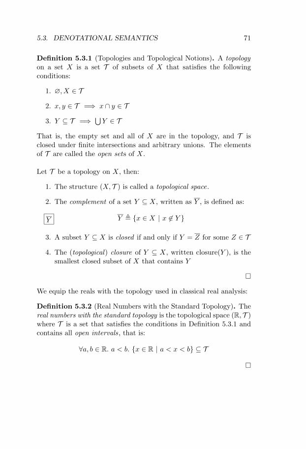
5.3. DENOTATIONAL SEMANTICS 71
Definition 5.3.1 (Topologies and Topological Notions). A topologyon a set X is a set T of subsets of X that satisfies the followingconditions:
1. ∅, X ∈ T
2. x, y ∈ T =⇒ x ∩ y ∈ T
3. Y ⊆ T =⇒⋃Y ∈ T
That is, the empty set and all of X are in the topology, and T isclosed under finite intersections and arbitrary unions. The elementsof T are called the open sets of X.
Let T be a topology on X, then:
1. The structure (X, T ) is called a topological space.
2. The complement of a set Y ⊆ X, written as Y , is defined as:
Y Y , {x ∈ X | x 6∈ Y }
3. A subset Y ⊆ X is closed if and only if Y = Z for some Z ∈ T
4. The (topological) closure of Y ⊆ X, written closure(Y ), is thesmallest closed subset of X that contains Y
�
We equip the reals with the topology used in classical real analysis:
Definition 5.3.2 (Real Numbers with the Standard Topology). Thereal numbers with the standard topology is the topological space (R, T )where T is a set that satisfies the conditions in Definition 5.3.1 andcontains all open intervals, that is:
∀a, b ∈ R. a < b. {x ∈ R | a < x < b} ⊆ T
�
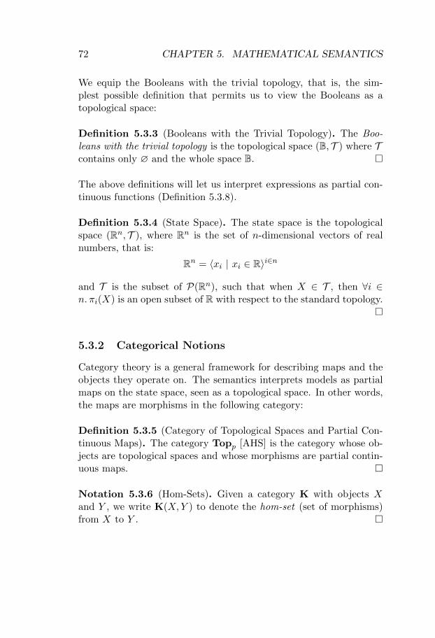
72 CHAPTER 5. MATHEMATICAL SEMANTICS
We equip the Booleans with the trivial topology, that is, the sim-plest possible definition that permits us to view the Booleans as atopological space:
Definition 5.3.3 (Booleans with the Trivial Topology). The Boo-leans with the trivial topology is the topological space (B, T ) where Tcontains only ∅ and the whole space B. �
The above definitions will let us interpret expressions as partial con-tinuous functions (Definition 5.3.8).
Definition 5.3.4 (State Space). The state space is the topologicalspace (Rn, T ), where Rn is the set of n-dimensional vectors of realnumbers, that is:
Rn = 〈xi | xi ∈ R〉i∈n
and T is the subset of P(Rn), such that when X ∈ T , then ∀i ∈n. πi(X) is an open subset of R with respect to the standard topology.
�
5.3.2 Categorical Notions
Category theory is a general framework for describing maps and theobjects they operate on. The semantics interprets models as partialmaps on the state space, seen as a topological space. In other words,the maps are morphisms in the following category:
Definition 5.3.5 (Category of Topological Spaces and Partial Con-tinuous Maps). The category Topp [AHS] is the category whose ob-jects are topological spaces and whose morphisms are partial contin-uous maps. �
Notation 5.3.6 (Hom-Sets). Given a category K with objects Xand Y , we write K(X,Y ) to denote the hom-set (set of morphisms)from X to Y . �
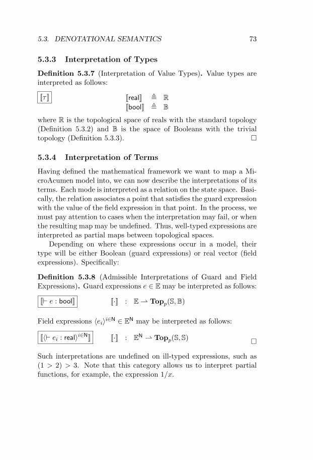
5.3. DENOTATIONAL SEMANTICS 73
5.3.3 Interpretation of Types
Definition 5.3.7 (Interpretation of Value Types). Value types areinterpreted as follows:
[[τ ]] [[real]] , R[[bool]] , B
where R is the topological space of reals with the standard topology(Definition 5.3.2) and B is the space of Booleans with the trivialtopology (Definition 5.3.3). �
5.3.4 Interpretation of Terms
Having defined the mathematical framework we want to map a Mi-croAcumen model into, we can now describe the interpretations of itsterms. Each mode is interpreted as a relation on the state space. Basi-cally, the relation associates a point that satisfies the guard expressionwith the value of the field expression in that point. In the process, wemust pay attention to cases when the interpretation may fail, or whenthe resulting map may be undefined. Thus, well-typed expressions areinterpreted as partial maps between topological spaces.
Depending on where these expressions occur in a model, theirtype will be either Boolean (guard expressions) or real vector (fieldexpressions). Specifically:
Definition 5.3.8 (Admissible Interpretations of Guard and FieldExpressions). Guard expressions e ∈ E may be interpreted as follows:
[[` e : bool]] [[·]] : E⇀ Topp(S,B)
Field expressions 〈ei〉i∈N ∈ EN may be interpreted as follows:
[[〈` ei : real〉i∈N]] [[·]] : EN ⇀ Topp(S, S) �
Such interpretations are undefined on ill-typed expressions, such as(1 > 2) > 3. Note that this category allows us to interpret partialfunctions, for example, the expression 1/x.
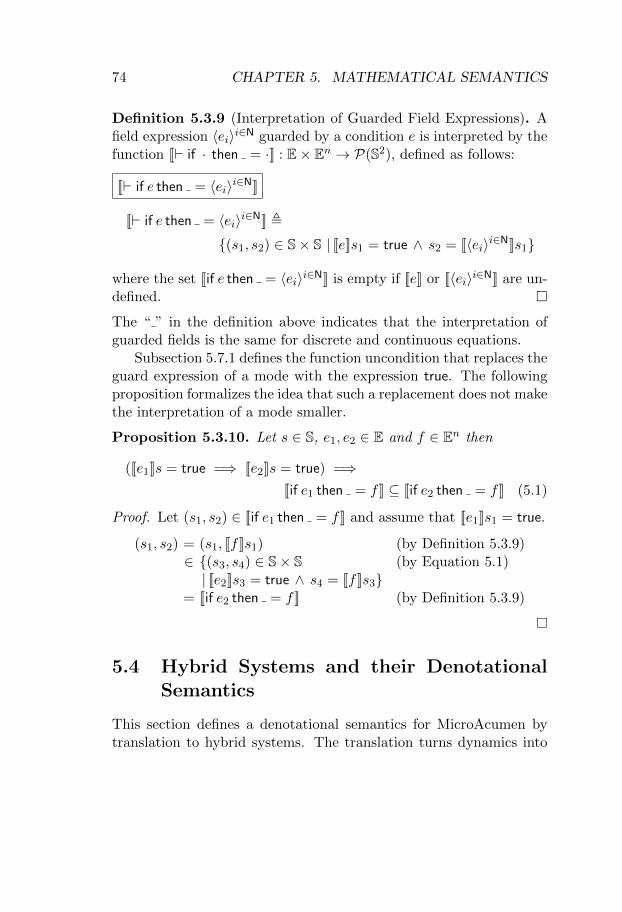
74 CHAPTER 5. MATHEMATICAL SEMANTICS
Definition 5.3.9 (Interpretation of Guarded Field Expressions). Afield expression 〈ei〉i∈N guarded by a condition e is interpreted by thefunction [[` if · then = ·]] : E× En → P(S2), defined as follows:
[[` if e then = 〈ei〉i∈N]]
[[` if e then = 〈ei〉i∈N]] ,
{(s1, s2) ∈ S× S | [[e]]s1 = true ∧ s2 = [[〈ei〉i∈N]]s1}
where the set [[if e then = 〈ei〉i∈N]] is empty if [[e]] or [[〈ei〉i∈N]] are un-defined. �
The “ ” in the definition above indicates that the interpretation ofguarded fields is the same for discrete and continuous equations.
Subsection 5.7.1 defines the function uncondition that replaces theguard expression of a mode with the expression true. The followingproposition formalizes the idea that such a replacement does not makethe interpretation of a mode smaller.
Proposition 5.3.10. Let s ∈ S, e1, e2 ∈ E and f ∈ En then
([[e1]]s = true =⇒ [[e2]]s = true) =⇒[[if e1 then = f ]] ⊆ [[if e2 then = f ]] (5.1)
Proof. Let (s1, s2) ∈ [[if e1 then = f ]] and assume that [[e1]]s1 = true.
(s1, s2) = (s1, [[f ]]s1) (by Definition 5.3.9)∈ {(s3, s4) ∈ S× S (by Equation 5.1)| [[e2]]s3 = true ∧ s4 = [[f ]]s3}
= [[if e2 then = f ]] (by Definition 5.3.9)
5.4 Hybrid Systems and their DenotationalSemantics
This section defines a denotational semantics for MicroAcumen bytranslation to hybrid systems. The translation turns dynamics into
5.4. DENOTATIONAL SEMANTICS 75
relations on the set state space S. These relations are used to definethe interpretation of hybrid systems as evolutions, which are closedsets of time-states. Evolutions will be used to state a conjecture aboutthe soundness of the operational semantics of MicroAcumen.
5.4.1 Hybrid Systems
A hybrid system [GST] is an abstract representation of how a statechanges over time, according to either discrete or continuous dynam-ics. This subsection defines a translation from MicroAcumen to hy-brid systems.
Definition 5.4.1 (Hybrid System). A hybrid system (F, J) ∈ H ona state space S = RN is a pair of binary relations F, J ⊆ S× S. �
The jump relation J represents the discrete dynamics, and the flowrelation F represents the continuous dynamics. These two relationsare interpreted differently: J is a simple mapping between states, Fspecifies a vector field by associating states with their derivatives. Forexample:
Example 5.4.2 (Sawtooth Wave Hybrid System). The sawtooth wavesystem can be modeled as a hybrid system as follows:
(F, J) = ({(x, 1) | x < 1}, {(x, 0) | x ≥ 1})
The flow and jump relations are sets of pairs of states. Next, we willsee how to obtain these sets given a MicroAcumen model.
5.4.2 Models as Hybrid Systems
This section gives a semantics to a MicroAcumen model by trans-lation into a hybrid system. It is obtained by translating each ofthe model’s modes, and combining the resulting hybrid systems. Inthe translation, discrete modes contribute to the jump relation andcontinuous modes to the flow relation.
76 CHAPTER 5. MATHEMATICAL SEMANTICS
Definition 5.4.3 (Interpretation of Models and Modes). A modelm ∈ Mµ is interpreted as a hybrid system H(m) using a functionH(·) : Mµ → H defined as follows:
H(m) H(·) : Mµ → HH(〈qi〉i∈N) , (
⋃i∈N Fi,
⋃i∈N Ji) where (Fi, Ji) = H(qi)
A mode q ∈ Q is interpreted as a hybrid system using a functionH(·) : Q→ H defined as follows:
H(q) H(·) : Q→ HH(if e then 〈x′i = ei〉i∈N) , ([[if e then = 〈ei〉i∈n]],∅)
H(if e then 〈x+i = ei〉i∈N) , (∅, [[if e then = 〈ei〉i∈n]])
�
Thus, the hybrid system of a model is the component-wise union ofthe relations obtained by translating its modes.
5.4.3 Valid Transitions
The key notion needed to define the denotational semantics is thetransition relation that relates states of a system as it evolves overtime. States may be related by flow (continuous) or jump (discrete)transitions. A flow transition relates two states through a differen-tiable map:
Definition 5.4.4 (Derivatives and Continuously Differentiable Maps).A map x : R→ Rn is continuously differentiable if the derivative
dx(t)
dt
dx(t)
dt, lim
h→0+
x(t+ h)− x(t)
h
is defined and is continuous over dom(x). We write C1(A,B) to de-note the set of once continuously differentiable maps from A to B,that is, for x ∈ C1(A,B), the derivative dx(t)
dt is defined on A. �
Using this notion we can now define the valid transitions for a hybridsystem.
5.4. DENOTATIONAL SEMANTICS 77
Definition 5.4.5 (Valid Transitions for a Hybrid System). The tran-
sition relation · δ- · : S × S → B for the hybrid system (F, J) andreal δ ≥ 0 is defined as follows
(F, J), s1δ- s2
(s1, s2) ∈ J
(F, J), s10- s2
δ > 0x ∈ C1([0, δ], S) x(0) = s1, x(δ) = s2∀t ∈ [0, δ]. (x(t), x′(t)) ∈ Flimt→0+ x
′(t)↓ ∧ limt→δ− x′(t)↓
(F, J), s1δ- s2
�
The two rules for valid transitions of a hybrid system correspond toits flows F and jumps J . The rule for jumps says that a transitionin zero time between two states is possible when these states are inthe jump relation. The rule for flow says that a transition betweentwo states in time δ > 0 is possible when these states are connectedby a continuously differentiable function x(t), such that this functionand its derivative x′(t) are in the flow relation, and the derivativeis defined for all t ∈ [0 .. δ]. We call x(t) a solution of an InitialValue Problem (IVP) defined by the triple (x′(t), x(0), δ), where x′(t)is called the field, x(0) the initial condition and δ the step.
Notation 5.4.6. For convenience, we omit the δ when its value isnot relevant. That is,
(F, J), s1 - s2
(F, J), s1 - s2 , ∃δ ≥ 0. (F, J), s1δ- s2
�
5.4.4 Evolutions
With the definition of the valid transitions for a hybrid system inhand, we can now define the behavior of a hybrid system over time,called its evolution:
78 CHAPTER 5. MATHEMATICAL SEMANTICS
Definition 5.4.7 (Evolution of a Hybrid System). The evolution ofa hybrid system (F, J) is a map [[(F, J)]] : Pclosed(S) → Pclosed(T × S)defined as the least fixpoint of a map F . For an initial set of statesS ⊆ S, the map F : Pclosed(T×S)→ Pclosed(T×S) is defined as follows:
F(I) = closure(({0}×S)∪{(t+δ, s2) | (t, s1) ∈ I ∧ (F, J), s1δ- s2})
�
An evolution for a hybrid system consists of sets of states that arereachable through the hybrid system at a given time. Any state inthe evolution is reachable from the initial state through a chain oftransitions (Definition 5.4.5).
5.5 Value Enclosures
Enclosures are computationally convenient subsets of the state spacefor a particular time step.
Definition 5.5.1 (Value Enclosure).
d ∈ D Value enclosures d ∈ D ⊂ Pclosed(S) that represent non-empty closed subsets of S for which d1 ⊆ d2 is decidable.
�
Value enclosures represent uncertainty about the state of the system.This uncertainty can come from measurement error, approximationerror, or from considering sets of configurations of a system at thesame time. Examples of concrete classes of enclosures are intervalboxes [War; Sun; MB2], parallelepipeds [Loh; Ned; Bar], and affineforms [DFS].
5.6 Timed Enclosures and their DenotationalSemantics
We now turn to the notion of timed enclosures, which will be used todefine the operational semantics. The definition relies on:
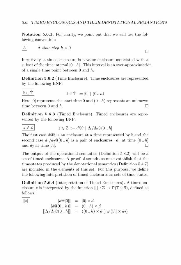
5.6. TIMED ENCLOSURES AND THEIR DENOTATIONAL SEMANTICS79
Notation 5.6.1. For clarity, we point out that we will use the fol-lowing convention:
h A time step h > 0�
Intuitively, a timed enclosure is a value enclosure associated with asubset of the time interval [0 .. h]. This interval is an over-approximationof a single time point between 0 and h.
Definition 5.6.2 (Time Enclosure). Time enclosures are representedby the following BNF:
t ∈ T t ∈ T ::= [0] | (0 .. h)
Here [0] represents the start time 0 and (0 .. h) represents an unknowntime between 0 and h. �
Definition 5.6.3 (Timed Enclosure). Timed enclosures are repre-sented by the following BNF:
z ∈ Z z ∈ Z ::= d@t | d1/d2@(0 .. h]
The first case d@t is an enclosure at a time represented by t and thesecond case d1/d2@(0 .. h] is a pair of enclosures: d1 at time (0 .. h]and d2 at time [h]. �
The output of the operational semantics (Definition 5.8.2) will be aset of timed enclosures. A proof of soundness must establish that thetime-states produced by the denotational semantics (Definition 5.4.7)are included in the elements of this set. For this purpose, we definethe following interpretation of timed enclosures as sets of time-states.
Definition 5.6.4 (Interpretation of Timed Enclosures). A timed en-closure z is interpreted by the function [[·]] : Z→ P(T×S), defined asfollows:
[[z]] [[d@[0]]] = [0]× d[[d@(0 .. h)]] = (0 .. h)× d
[[d1/d2@(0 .. h]]] = ((0 .. h)× d1) ] ([h]× d2)
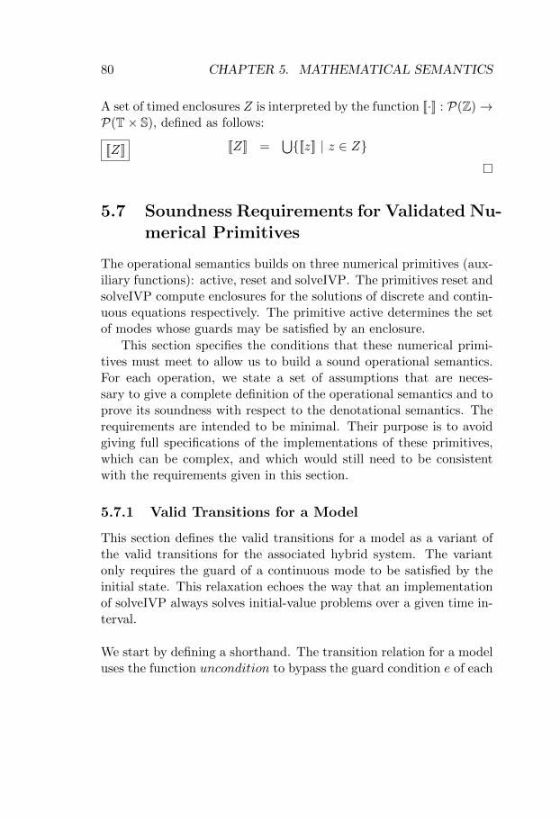
80 CHAPTER 5. MATHEMATICAL SEMANTICS
A set of timed enclosures Z is interpreted by the function [[·]] : P(Z)→P(T× S), defined as follows:
[[Z]] [[Z]] =⋃{[[z]] | z ∈ Z}
�
5.7 Soundness Requirements for Validated Nu-merical Primitives
The operational semantics builds on three numerical primitives (aux-iliary functions): active, reset and solveIVP. The primitives reset andsolveIVP compute enclosures for the solutions of discrete and contin-uous equations respectively. The primitive active determines the setof modes whose guards may be satisfied by an enclosure.
This section specifies the conditions that these numerical primi-tives must meet to allow us to build a sound operational semantics.For each operation, we state a set of assumptions that are neces-sary to give a complete definition of the operational semantics and toprove its soundness with respect to the denotational semantics. Therequirements are intended to be minimal. Their purpose is to avoidgiving full specifications of the implementations of these primitives,which can be complex, and which would still need to be consistentwith the requirements given in this section.
5.7.1 Valid Transitions for a Model
This section defines the valid transitions for a model as a variant ofthe valid transitions for the associated hybrid system. The variantonly requires the guard of a continuous mode to be satisfied by theinitial state. This relaxation echoes the way that an implementationof solveIVP always solves initial-value problems over a given time in-terval.
We start by defining a shorthand. The transition relation for a modeluses the function uncondition to bypass the guard condition e of each
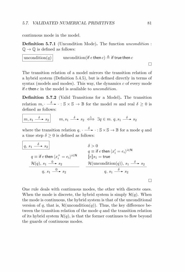
5.7. VALIDATED NUMERICAL PRIMITIVES 81
continuous mode in the model.
Definition 5.7.1 (Uncondition Mode). The function uncondition :Q→ Q is defined as follows:
uncondition(q) uncondition(if e then c) , if true then c
�
The transition relation of a model mirrors the transition relation ofa hybrid system (Definition 5.4.5), but is defined directly in terms ofsyntax (models and modes). This way, the dynamics c of every modeif e then c in the model is available to uncondition.
Definition 5.7.2 (Valid Transitions for a Model). The transition
relation m, · δ- · : S × S → B for the model m and real δ ≥ 0 isdefined as follows:
m, s1δ- s2 m, s1
δ- s2M⇐⇒ ∃q ∈ m. q, s1 δ- s2
where the transition relation q, · δ- · : S×S→ B for a mode q anda time step δ ≥ 0 is defined as follows:
q, s1δ- s2
q ≡ if e then 〈x+i = ei〉i∈N
H(q), s10- s2
q, s10- s2
δ > 0q ≡ if e then 〈x′i = ei〉i∈N[[e]]s1 = true
H(uncondition(q)), s1δ- s2
q, s1δ- s2
�
One rule deals with continuous modes, the other with discrete ones.When the mode is discrete, the hybrid system is simply H(q). Whenthe mode is continuous, the hybrid system is that of the unconditionalversion of q, that is, H(uncondition(q)). Thus, the key difference be-tween the transition relation of the mode q and the transition relationof its hybrid system H(q), is that the former continues to flow beyondthe guards of continuous modes.
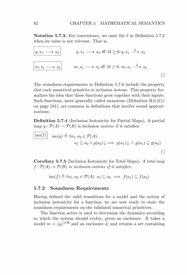
82 CHAPTER 5. MATHEMATICAL SEMANTICS
Notation 5.7.3. For convenience, we omit the δ in Definition 5.7.2when its value is not relevant. That is,
q, s1 - s2 q, s1 - s2 iff ∃δ ≥ 0. q, s1δ- s2
m, s1 - s2 m, s1 - s2 iff ∃δ ≥ 0. m, s1δ- s2
�
The soundness requirements in Definition 5.7.6 include the propertythat each numerical primitive is inclusion isotone. This property for-malizes the idea that these functions grow together with their inputs.Such functions, more generally called monotone (Definition B.0.2(1)on page 181), are common in definitions that involve sound approxi-mations.
Definition 5.7.4 (Inclusion Isotonicity for Partial Maps). A partialmap g : P(A) ⇀ P(B) is inclusion isotone if it satisfies:
iso(f) iso(g) , ∀a1, a2 ∈ P(A).
a1 ⊆ a2 ∧ g(a2)↓ =⇒ g(a1)↓ ∧ g(a1) ⊆ g(a2)
�
Corollary 5.7.5 (Inclusion Isotonicity for Total Maps). A total mapf : P(A)→ P(B) is inclusion isotone if it satisfies:
iso(f) , ∀a1, a2 ∈ P(A). a1 ⊆ a2 =⇒ f(a1) ⊆ f(a2)
5.7.2 Soundness Requirements
Having defined the valid transitions for a model and the notion ofinclusion isotonicity for a function, we are now ready to state thesoundness requirements on the validated numerical primitives.
The function active is used to determine the dynamics accordingto which the system should evolve, given an enclosure. It takes amodel m = 〈qi〉i∈N and an enclosure d, and returns a set containing
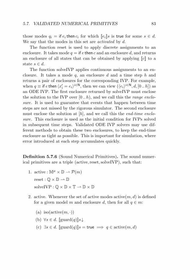
5.7. VALIDATED NUMERICAL PRIMITIVES 83
those modes qi = if ei then ci for which [[ei]]s is true for some s ∈ d.We say that the modes in this set are activated by d.
The function reset is used to apply discrete assignments to anenclosure. It takes mode q = if e then c and an enclosure d, and returnsan enclosure of all states that can be obtained by applying [[c]] to astate s ∈ d.
The function solveIVP applies continuous assignments to an en-closure. It takes a mode q, an enclosure d and a time step h andreturns a pair of enclosures for the corresponding IVP. For example,when q ≡ if e then 〈x′i = ei〉i∈N, then we can view (〈ei〉i∈N, d, [0 .. h]) asan ODE IVP. The first enclosure returned by solveIVP must enclosethe solution to the IVP over [0 .. h), and we call this the range enclo-sure. It is used to guarantee that events that happen between timesteps are not missed by the rigorous simulator. The second enclosuremust enclose the solution at [h], and we call this the end-time enclo-sure. This enclosure is used as the initial condition for IVPs solvedin subsequent time steps. Validated ODE IVP solvers may use dif-ferent methods to obtain these two enclosures, to keep the end-timeenclosure as tight as possible. This is important for simulation, whereerror introduced at each step accumulates quickly.
Definition 5.7.6 (Sound Numerical Primitives). The sound numer-ical primitives are a triple (active, reset, solveIVP), such that:
1. active : Mµ × D⇀ P(m)
reset : Q× D⇀ D
solveIVP : Q× D× T⇀ D× D
2. active. Whenever the set of active modes active(m, d) is definedfor a given model m and enclosure d, then for all q ∈ m:
(a) iso(active(m, ·))(b) ∀s ∈ d. [[guard(q)]]s↓(c) ∃s ∈ d. [[guard(q)]]s = true =⇒ q ∈ active(m, d)
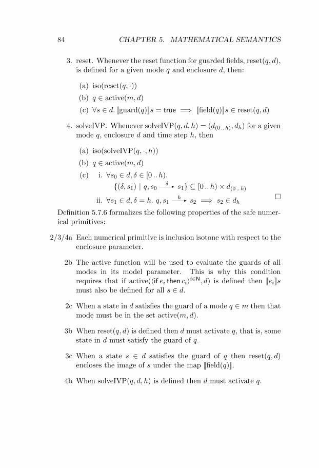
84 CHAPTER 5. MATHEMATICAL SEMANTICS
3. reset. Whenever the reset function for guarded fields, reset(q, d),is defined for a given mode q and enclosure d, then:
(a) iso(reset(q, ·))(b) q ∈ active(m, d)
(c) ∀s ∈ d. [[guard(q)]]s = true =⇒ [[field(q)]]s ∈ reset(q, d)
4. solveIVP. Whenever solveIVP(q, d, h) = (d(0 .. h), dh) for a givenmode q, enclosure d and time step h, then
(a) iso(solveIVP(q, ·, h))
(b) q ∈ active(m, d)
(c) i. ∀s0 ∈ d, δ ∈ [0 .. h).
{(δ, s1) | q, s0 δ- s1} ⊆ [0 .. h)× d(0 .. h)ii. ∀s1 ∈ d, δ = h. q, s1
h- s2 =⇒ s2 ∈ dh �
Definition 5.7.6 formalizes the following properties of the safe numer-ical primitives:
2/3/4a Each numerical primitive is inclusion isotone with respect to theenclosure parameter.
2b The active function will be used to evaluate the guards of allmodes in its model parameter. This is why this conditionrequires that if active(〈if ei then ci〉i∈N, d) is defined then [[ei]]smust also be defined for all s ∈ d.
2c When a state in d satisfies the guard of a mode q ∈ m then thatmode must be in the set active(m, d).
3b When reset(q, d) is defined then d must activate q, that is, somestate in d must satisfy the guard of q.
3c When a state s ∈ d satisfies the guard of q then reset(q, d)encloses the image of s under the map [[field(q)]].
4b When solveIVP(q, d, h) is defined then d must activate q.
5.8. OPERATIONAL SEMANTICS 85
4(c)i Any state reachable from d by the transition relation of themode q (Definition 5.7.2) within time h is included in the en-closure d(0 .. h).
4(c)ii Any state reachable from d by the transition relation of themode q (Definition 5.7.2) in exactly time h is included in theenclosure dh.
5.8 Operational Semantics
This section presents an operational semantics for MicroAcumen,specified by rules that follow the syntax. Notable efforts that usethis approach to specify a hybrid systems language include opera-tional semantics for Simulink [BC], the Compositional InterchangeFormat [AvBR] and the Modeling Kernel Language [Bro]. Otherrelated efforts focus on specific issues, such as choosing appropriatedomains for time and the state space in an operational semantics [BF].
Unlike these examples, the goal of our operational semantics isto produce enclosures, which requires propagating error bounds pro-vided by auxiliary functions, and combining these with additionalerror incurred by the operational semantics itself. A comprehensivetreatment of such aspects of semantics has been given in the contextof domain theory [EP], but without a clear connection to an existingimplementation. Specifications of algorithms that take approxima-tion into account, and for which there are implementations, can befound in literature on model checking [ADI; Gao], though these typ-ically specify algorithms in pseudocode rather than by rules. Thesemantics presented in this chapter is in many ways similar to the op-erational semantics for TinyHCC developed in the thesis of DaisukeIshii [Ish]. A key difference is that our work is explicit about the wayin which the discretization of time affects the precision of enclosures(the case t = (0 .. h) in the Continuous rule of Figure 5.5). Furtherstudy of the relationship between these languages and their semanticsis part of our future work.
The operational semantics is defined in terms of two functions:
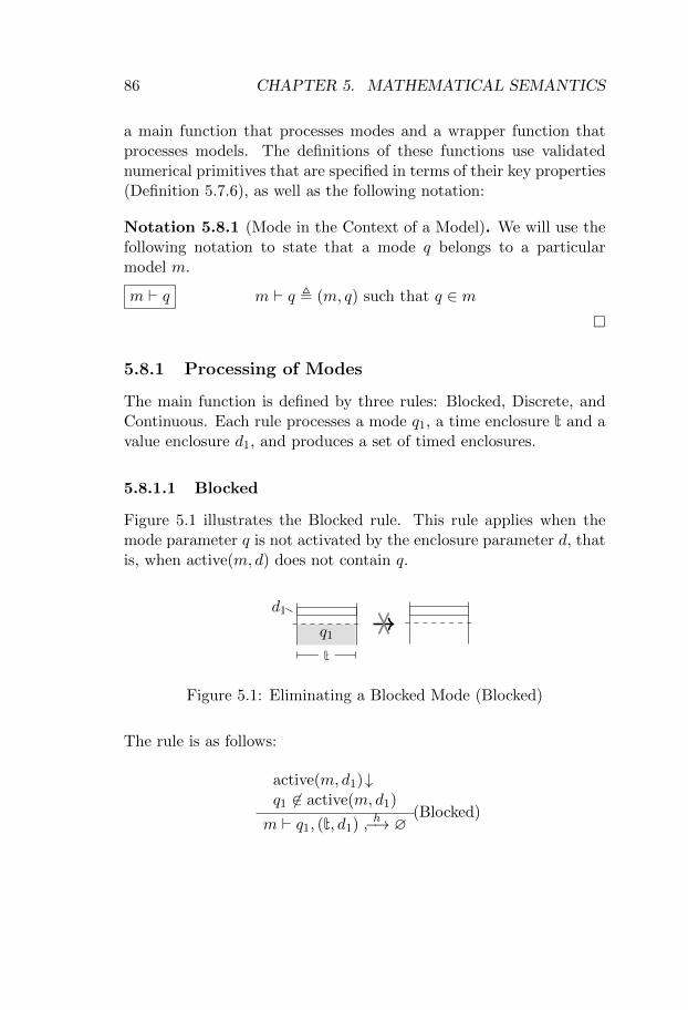
86 CHAPTER 5. MATHEMATICAL SEMANTICS
a main function that processes modes and a wrapper function thatprocesses models. The definitions of these functions use validatednumerical primitives that are specified in terms of their key properties(Definition 5.7.6), as well as the following notation:
Notation 5.8.1 (Mode in the Context of a Model). We will use thefollowing notation to state that a mode q belongs to a particularmodel m.
m ` q m ` q , (m, q) such that q ∈ m�
5.8.1 Processing of Modes
The main function is defined by three rules: Blocked, Discrete, andContinuous. Each rule processes a mode q1, a time enclosure t and avalue enclosure d1, and produces a set of timed enclosures.
5.8.1.1 Blocked
Figure 5.1 illustrates the Blocked rule. This rule applies when themode parameter q is not activated by the enclosure parameter d, thatis, when active(m, d) does not contain q.
q1
d1
t
Figure 5.1: Eliminating a Blocked Mode (Blocked)
The rule is as follows:
active(m, d1)↓q1 6∈ active(m, d1)
m ` q1, (t, d1) h↪−→ ∅(Blocked)
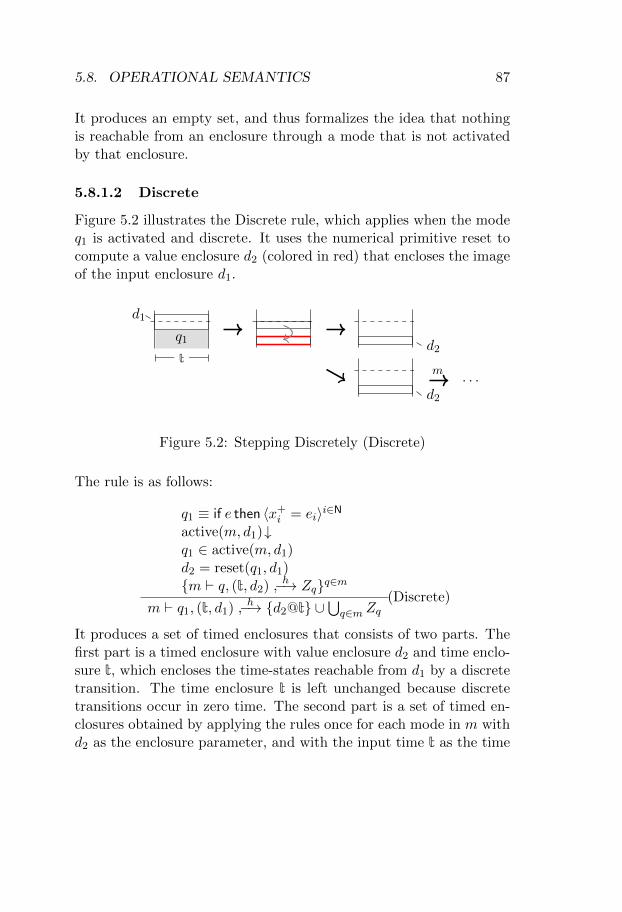
5.8. OPERATIONAL SEMANTICS 87
It produces an empty set, and thus formalizes the idea that nothingis reachable from an enclosure through a mode that is not activatedby that enclosure.
5.8.1.2 Discrete
Figure 5.2 illustrates the Discrete rule, which applies when the modeq1 is activated and discrete. It uses the numerical primitive reset tocompute a value enclosure d2 (colored in red) that encloses the imageof the input enclosure d1.
d1
t
q1 d2
d2
m. . .
Figure 5.2: Stepping Discretely (Discrete)
The rule is as follows:
q1 ≡ if e then 〈x+i = ei〉i∈Nactive(m, d1)↓q1 ∈ active(m, d1)d2 = reset(q1, d1){m ` q, (t, d2) h↪−→ Zq}q∈m
m ` q1, (t, d1) h↪−→ {d2@t} ∪⋃q∈m Zq
(Discrete)
It produces a set of timed enclosures that consists of two parts. Thefirst part is a timed enclosure with value enclosure d2 and time enclo-sure t, which encloses the time-states reachable from d1 by a discretetransition. The time enclosure t is left unchanged because discretetransitions occur in zero time. The second part is a set of timed en-closures obtained by applying the rules once for each mode in m withd2 as the enclosure parameter, and with the input time t as the time
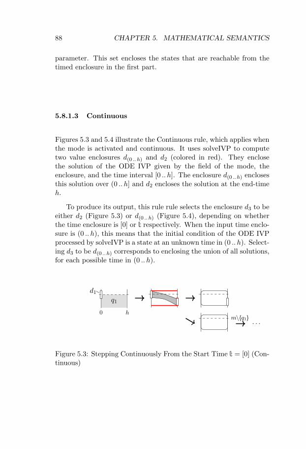
88 CHAPTER 5. MATHEMATICAL SEMANTICS
parameter. This set encloses the states that are reachable from thetimed enclosure in the first part.
5.8.1.3 Continuous
Figures 5.3 and 5.4 illustrate the Continuous rule, which applies whenthe mode is activated and continuous. It uses solveIVP to computetwo value enclosures d(0 .. h) and d2 (colored in red). They enclosethe solution of the ODE IVP given by the field of the mode, theenclosure, and the time interval [0 .. h]. The enclosure d(0 .. h) enclosesthis solution over (0 .. h] and d2 encloses the solution at the end-timeh.
To produce its output, this rule rule selects the enclosure d3 to beeither d2 (Figure 5.3) or d(0 .. h) (Figure 5.4), depending on whetherthe time enclosure is [0] or t respectively. When the input time enclo-sure is (0 .. h), this means that the initial condition of the ODE IVPprocessed by solveIVP is a state at an unknown time in (0 .. h). Select-ing d3 to be d(0 .. h) corresponds to enclosing the union of all solutions,for each possible time in (0 .. h).
d1
0 h
q1
m\{q1}. . .
Figure 5.3: Stepping Continuously From the Start Time t = [0] (Con-tinuous)
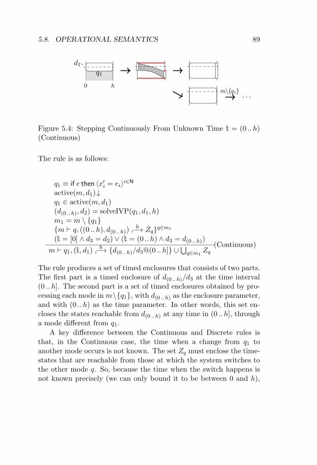
5.8. OPERATIONAL SEMANTICS 89
d1
0 h
q1
m\{q1}. . .
Figure 5.4: Stepping Continuously From Unknown Time t = (0 .. h)(Continuous)
The rule is as follows:
q1 ≡ if e then 〈x′i = ei〉i∈Nactive(m, d1)↓q1 ∈ active(m, d1)(d(0 .. h), d2) = solveIVP(q1, d1, h)
m1 = m \ {q1}{m ` q, ((0 .. h), d(0 .. h))
h↪−→ Zq}q∈m1
(t = [0] ∧ d3 = d2) ∨ (t = (0 .. h) ∧ d3 = d(0 .. h))
m ` q1, (t, d1) h↪−→ {d(0 .. h)/d3@(0 .. h]} ∪⋃q∈m1
Zq(Continuous)
The rule produces a set of timed enclosures that consists of two parts.The first part is a timed enclosure of d(0 .. h)/d3 at the time interval(0 .. h]. The second part is a set of timed enclosures obtained by pro-cessing each mode in m\{q1}, with d(0 .. h) as the enclosure parameter,and with (0 .. h) as the time parameter. In other words, this set en-closes the states reachable from d(0 .. h) at any time in (0 .. h], througha mode different from q1.
A key difference between the Continuous and Discrete rules isthat, in the Continuous case, the time when a change from q1 toanother mode occurs is not known. The set Zq must enclose the time-states that are reachable from those at which the system switches tothe other mode q. So, because the time when the switch happens isnot known precisely (we can only bound it to be between 0 and h),
90 CHAPTER 5. MATHEMATICAL SEMANTICS
the state is also not known precisely (we can only bound it to be inthe range of the solution over (0 .. h)). Because the value enclosured(0 .. h) encloses the range of the solution over (0 .. h), this enclosureis used as a safe approximation of the true state at which the systemswitched to the other mode.
5.8.2 Processing of Models
The function m, d h↪−→ Z is defined by a rule that takes a model m,an enclosure d and a time step h, and returns a set of timed states Z:
{m ` q, ([0], d) h↪−→ Zq}q∈m
m, d h↪−→ {d@[0]} ∪⋃q∈m Zq
This set consists of the timed enclosure d@[0] (the initial state ofthe system) and a union of sets of timed enclosures produced by themain function m ` q, (·, ·) ·↪−→ · (the states that are reachable fromthe initial state by each mode q ∈ m).
We combine the definitions of the main function (that processes modes)and wrapper function (that processes models) into an operational se-mantics for MicroAcumen:
Definition 5.8.2 (Operational Semantics). The operational seman-tics for a model is given by the function · ↪−→ · : Mµ×D×T⇀ Z andthe function · ↪−→ · : Q× T×D×T⇀ Pf (Z) defined in Figure 5.5. �
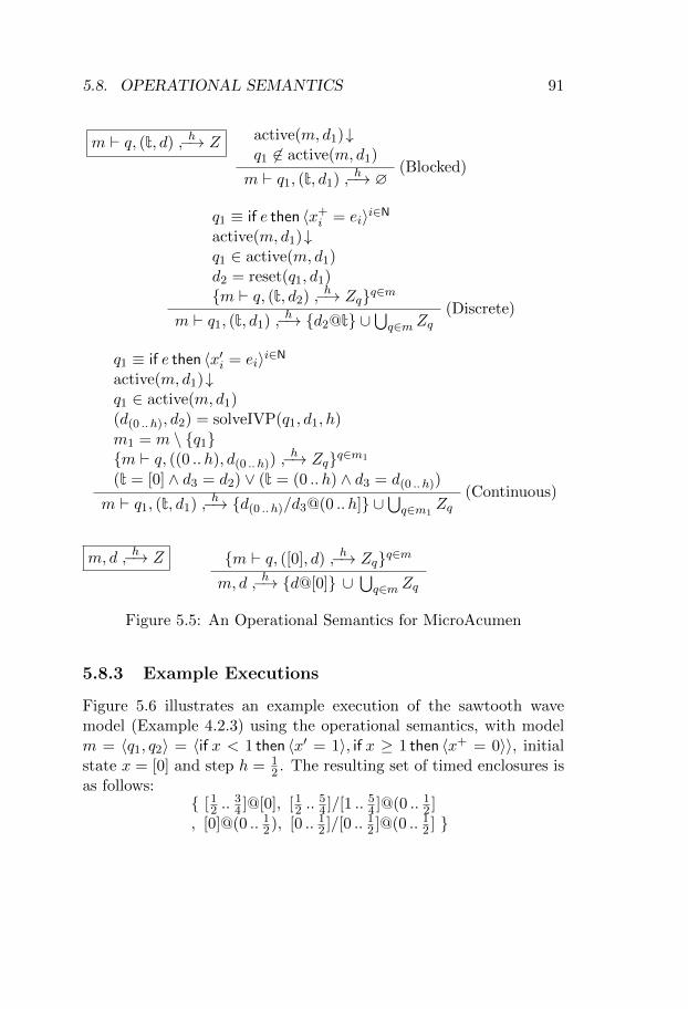
5.8. OPERATIONAL SEMANTICS 91
m ` q, (t, d) h↪−→ Z active(m, d1)↓q1 6∈ active(m, d1)
m ` q1, (t, d1) h↪−→ ∅(Blocked)
q1 ≡ if e then 〈x+i = ei〉i∈Nactive(m, d1)↓q1 ∈ active(m, d1)d2 = reset(q1, d1){m ` q, (t, d2) h↪−→ Zq}q∈m
m ` q1, (t, d1) h↪−→ {d2@t} ∪⋃q∈m Zq
(Discrete)
q1 ≡ if e then 〈x′i = ei〉i∈Nactive(m, d1)↓q1 ∈ active(m, d1)(d(0 .. h), d2) = solveIVP(q1, d1, h)
m1 = m \ {q1}{m ` q, ((0 .. h), d(0 .. h))
h↪−→ Zq}q∈m1
(t = [0] ∧ d3 = d2) ∨ (t = (0 .. h) ∧ d3 = d(0 .. h))
m ` q1, (t, d1) h↪−→ {d(0 .. h)/d3@(0 .. h]} ∪⋃q∈m1
Zq(Continuous)
m, d h↪−→ Z {m ` q, ([0], d) h↪−→ Zq}q∈m
m, d h↪−→ {d@[0]} ∪⋃q∈m Zq
Figure 5.5: An Operational Semantics for MicroAcumen
5.8.3 Example Executions
Figure 5.6 illustrates an example execution of the sawtooth wavemodel (Example 4.2.3) using the operational semantics, with modelm = 〈q1, q2〉 = 〈if x < 1 then 〈x′ = 1〉, if x ≥ 1 then 〈x+ = 0〉〉, initialstate x = [0] and step h = 1
2 . The resulting set of timed enclosures isas follows:
{ [12 ..34 ]@[0], [12 ..
54 ]/[1 .. 54 ]@(0 .. 12 ]
, [0]@(0 .. 12), [0 .. 12 ]/[0 .. 12 ]@(0 .. 12 ] }
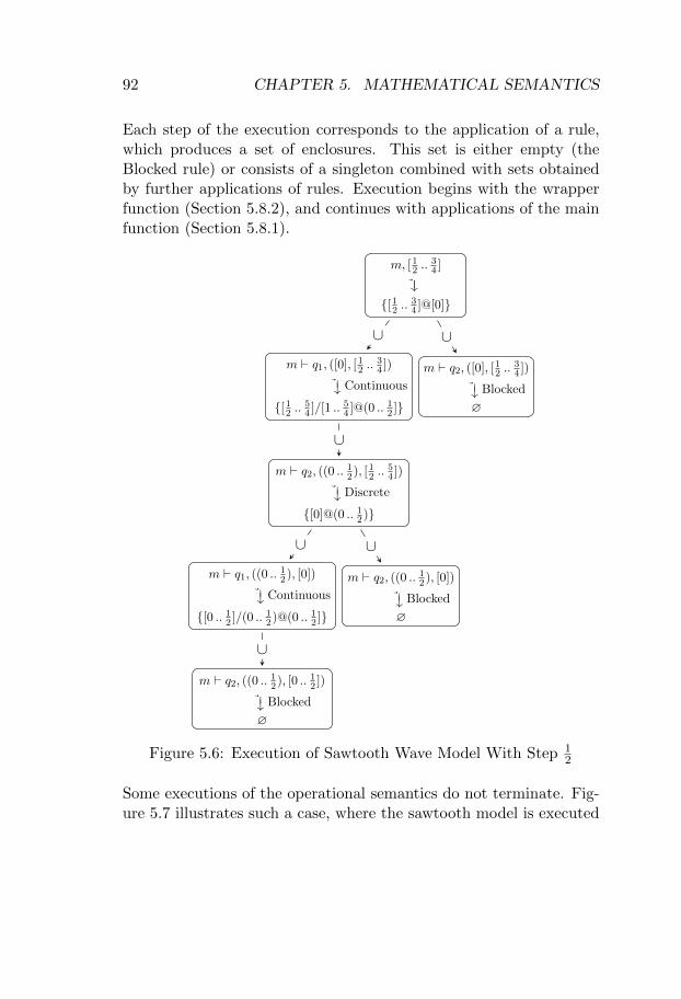
92 CHAPTER 5. MATHEMATICAL SEMANTICS
Each step of the execution corresponds to the application of a rule,which produces a set of enclosures. This set is either empty (theBlocked rule) or consists of a singleton combined with sets obtainedby further applications of rules. Execution begins with the wrapperfunction (Section 5.8.2), and continues with applications of the mainfunction (Section 5.8.1).
m, [12 ..34 ]
↪−→
{[12 ..34 ]@[0]}
m ` q1, ([0], [12 ..34 ])
Continuous
↪−→
{[12 ..54 ]/[1 .. 54 ]@(0 .. 12 ]}
m ` q2, ([0], [12 ..34 ])
Blocked
↪−→
∅
m ` q2, ((0 .. 12), [12 ..54 ])
Discrete
↪−→
{[0]@(0 .. 12)}
m ` q1, ((0 .. 12), [0])
Continuous
↪−→
{[0 .. 12 ]/(0 .. 12)@(0 .. 12 ]}
m ` q2, ((0 .. 12), [0])
Blocked
↪−→
∅
m ` q2, ((0 .. 12), [0 .. 12 ])
Blocked
↪−→
∅
∪∪
∪
∪ ∪
∪
Figure 5.6: Execution of Sawtooth Wave Model With Step 12
Some executions of the operational semantics do not terminate. Fig-ure 5.7 illustrates such a case, where the sawtooth model is executed
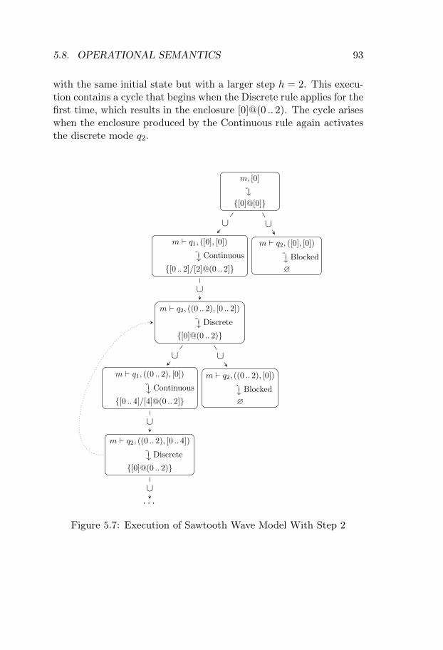
5.8. OPERATIONAL SEMANTICS 93
with the same initial state but with a larger step h = 2. This execu-tion contains a cycle that begins when the Discrete rule applies for thefirst time, which results in the enclosure [0]@(0 .. 2). The cycle ariseswhen the enclosure produced by the Continuous rule again activatesthe discrete mode q2.
m, [0]
↪−→{[0]@[0]}
m ` q1, ([0], [0])
Continuous
↪−→
{[0 .. 2]/[2]@(0 .. 2]}
m ` q2, ([0], [0])
Blocked
↪−→
∅
m ` q2, ((0 .. 2), [0 .. 2])
Discrete
↪−→
{[0]@(0 .. 2)}
m ` q1, ((0 .. 2), [0])
Continuous
↪−→
{[0 .. 4]/[4]@(0 .. 2]}
m ` q2, ((0 .. 2), [0])
Blocked
↪−→
∅
m ` q2, ((0 .. 2), [0 .. 4])
Discrete
↪−→
{[0]@(0 .. 2)}
. . .
∪∪
∪
∪ ∪
∪
∪
Figure 5.7: Execution of Sawtooth Wave Model With Step 2
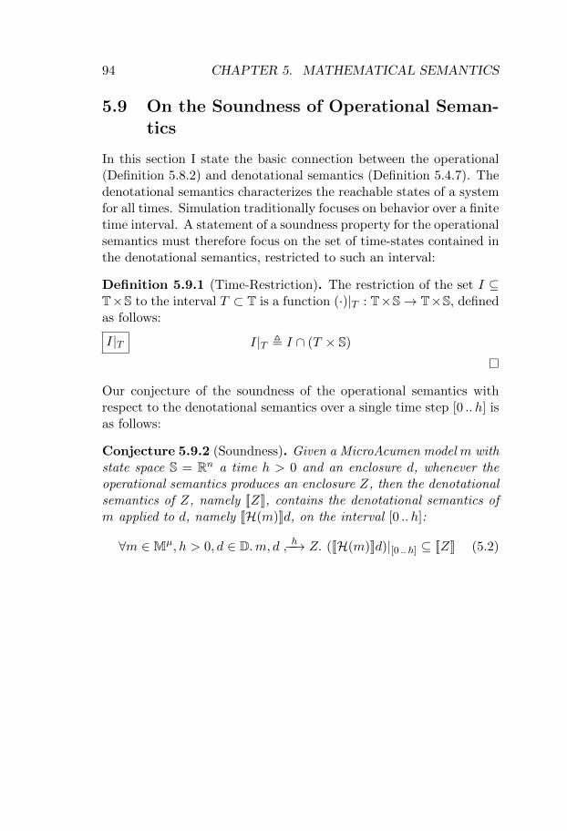
94 CHAPTER 5. MATHEMATICAL SEMANTICS
5.9 On the Soundness of Operational Seman-tics
In this section I state the basic connection between the operational(Definition 5.8.2) and denotational semantics (Definition 5.4.7). Thedenotational semantics characterizes the reachable states of a systemfor all times. Simulation traditionally focuses on behavior over a finitetime interval. A statement of a soundness property for the operationalsemantics must therefore focus on the set of time-states contained inthe denotational semantics, restricted to such an interval:
Definition 5.9.1 (Time-Restriction). The restriction of the set I ⊆T×S to the interval T ⊂ T is a function (·)|T : T×S→ T×S, definedas follows:
I|T I|T , I ∩ (T × S)
�
Our conjecture of the soundness of the operational semantics withrespect to the denotational semantics over a single time step [0 .. h] isas follows:
Conjecture 5.9.2 (Soundness). Given a MicroAcumen model m withstate space S = Rn a time h > 0 and an enclosure d, whenever theoperational semantics produces an enclosure Z, then the denotationalsemantics of Z, namely [[Z]], contains the denotational semantics ofm applied to d, namely [[H(m)]]d, on the interval [0 .. h]:
∀m ∈Mµ, h > 0, d ∈ D.m, d h↪−−→ Z. ([[H(m)]]d)|[0 .. h] ⊆ [[Z]] (5.2)

Part III
Applications
95

Chapter 6
Implementation
In this chapter we review the implementation of the Acumen lan-guage, which was developed jointly by Halmstad University and RiceUniversity. The rest of this chapter is structured as follows. First, wereview the two semantics that the implementation supports. Second,we review the user interfaces into which the modeling and simulationenvironment is integrated. Third, we review the organization of thecode base and its key components. Last, we review two approachesto testing that are used in Acumen’s automated test suite.
6.1 Introduction
The implementation was partly developed before the theory presentedin Chapters 4 and 5, and partly in parallel with it. There were threemain reasons for doing so. First, the implementation allowed usto develop an understanding of the characteristics of both the tra-ditional and validated numerics that hybrid systems simulators canbuild upon. Second, the implementation served as a testbed for exper-imenting with the syntax and user interface. This led us to a small butflexible syntax that translates smoothly into the core syntax in termsof which the formal semantics is defined, and a user interface thatsupports features such as 3D visualization, which are vital for pro-ductivity when simulating large systems. Third, the implementation
97
98 CHAPTER 6. IMPLEMENTATION
allowed us to develop a collection of more than 500 example modelsof hybrid systems1. This collection contains both small models thatserve as benchmarks for specific semantic features (e.g. variants of abouncing ball), and large models that test the expressivity of the lan-guage and performance of the semantics (e.g. the model that Chapter7 describes). Having access to these examples helped us identify thecore features of a hybrid systems formalism, and provided us withongoing feedback on design choices.
As a result of developing the theory in parallel with the imple-mentation, there are places where they are not in full correspondence.There are two main differences. First, the implementation does notperform the translation into the core syntax before simulation, butinstead performs an analogous transformation before each simulationstep. Second, the implementation supports some syntactic and se-mantic features that have not yet been formalized in the theoreticalframework presented in the thesis. This includes support for sub-models, and support for simulating Zeno systems [KTB+].
The simulation results presented in this thesis can be reproducedusing the 2016 08 30 release of Acumen2 [aR], which is freely avail-able, as open source software. The models are included in the distri-bution under examples/05_Language_Research/24_ISO26262 andexamples/05_Language_Research/26_Convergence.
6.2 Traditional and Rigorous Simulation Se-mantics
Two kinds of interpreters that are included in the implementation.The first kind implements the traditional semantics, which uses floating-point numbers to represent real numbers and is based on traditionalnumerical ODE IVP solvers, such as 4th order Runge-Kutta and arbi-trary order Taylor Series integrators. The traditional semantics is themost complete and most widely used semantics, due to its predictable
1These models are available in the distribution [aR], under examples.2The “2015 Enclosure” option must be selected in the Semantics menu.
6.3. COMMAND-LINE INTERFACE (CLI) 99
performance and support for features such as 3D visualization. It hasplayed a crucial role in allowing us to explore the language designspace and to converge on an expressive, minimal syntax for model-ing hybrid systems and on a formal (exact) semantics for solutions.Among other design choices, it allowed us to make an early decisionto support the notion of super-dense time, first introduced in the ver-ification literature [MMP], and later advocated by Liu, Matsikoudisand Lee [LML]. This notion facilitates modeling of discrete subsys-tems with multiple idealized (zero time) and externally observableinternal transitions.
The second kind of semantics supported by the implementationis the enclosure semantics, which allows rigorous simulation using asubset of the full Acumen language. This semantics is intended toproduce rigorous over-approximations (guaranteed upper and lowerbounds) for all simulations [DEB+; KTB+]. A model of the subset ofAcumen supported by the enclosure simulation semantics is formal-ized in Chapter 5. The operational semantics in Figure 5.5 modelsthe behavior of this interpreter.
Acumen is both a language and an integrated modeling environ-ment that includes a code editor, interpreters, and facilities for vi-sualization. The implementation provides two main ways to interactwith an Acumen model.
6.3 Command-Line Interface (CLI)
The Command Line Interface (CLI) is a standard textual interfacefor executing models in a terminal or from a script. Using the CLI itis possible to trace the states of a model during a simulation, measurethe time it takes to execute a model, and record reference output filesfor the automated tests, among other things. To see all the avail-able commands, the --full-help flag must be passed when startingAcumen in a terminal:
java -jar acumen.jar --full-help
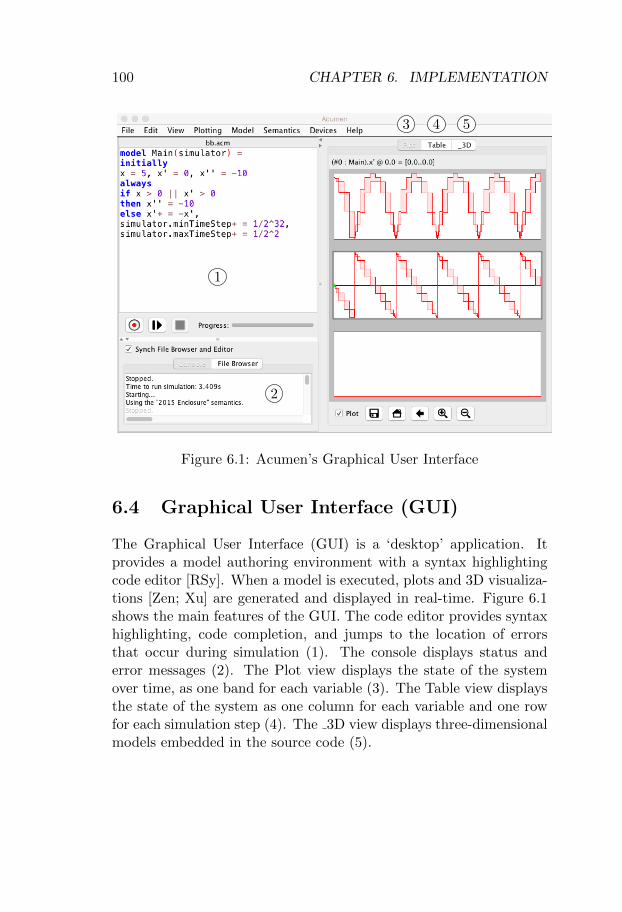
100 CHAPTER 6. IMPLEMENTATION
1
2
3 4 5
Figure 6.1: Acumen’s Graphical User Interface
6.4 Graphical User Interface (GUI)
The Graphical User Interface (GUI) is a ‘desktop’ application. Itprovides a model authoring environment with a syntax highlightingcode editor [RSy]. When a model is executed, plots and 3D visualiza-tions [Zen; Xu] are generated and displayed in real-time. Figure 6.1shows the main features of the GUI. The code editor provides syntaxhighlighting, code completion, and jumps to the location of errorsthat occur during simulation (1). The console displays status anderror messages (2). The Plot view displays the state of the systemover time, as one band for each variable (3). The Table view displaysthe state of the system as one column for each variable and one rowfor each simulation step (4). The 3D view displays three-dimensionalmodels embedded in the source code (5).
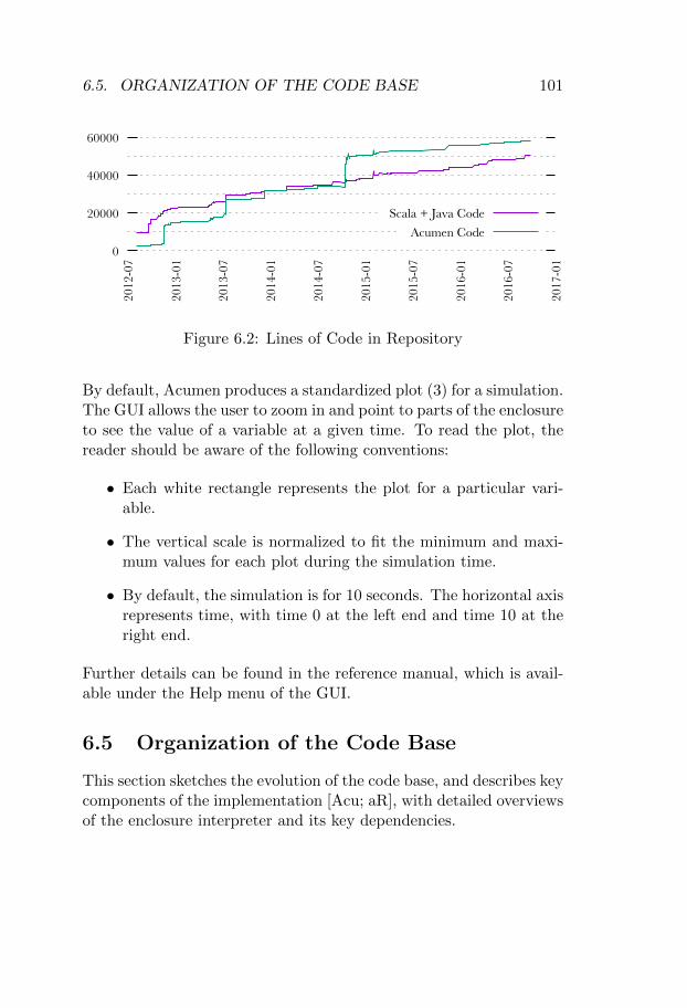
6.5. ORGANIZATION OF THE CODE BASE 101
0
20000
40000
600002012-07
2013-01
2013-07
2014-01
2014-07
2015-01
2015-07
2016-01
2016-07
2017-01
Scala + Java CodeAcumen Code
Figure 6.2: Lines of Code in Repository
By default, Acumen produces a standardized plot (3) for a simulation.The GUI allows the user to zoom in and point to parts of the enclosureto see the value of a variable at a given time. To read the plot, thereader should be aware of the following conventions:
• Each white rectangle represents the plot for a particular vari-able.
• The vertical scale is normalized to fit the minimum and maxi-mum values for each plot during the simulation time.
• By default, the simulation is for 10 seconds. The horizontal axisrepresents time, with time 0 at the left end and time 10 at theright end.
Further details can be found in the reference manual, which is avail-able under the Help menu of the GUI.
6.5 Organization of the Code Base
This section sketches the evolution of the code base, and describes keycomponents of the implementation [Acu; aR], with detailed overviewsof the enclosure interpreter and its key dependencies.
102 CHAPTER 6. IMPLEMENTATION
Figure 6.2 shows the evolution of the code base in terms of sourcecode lines checked-in to the Acumen source code repository [Rep],between July 2017 and October 2016. The figure shows both the sizeof the implementation Scala and Java code, and Acumen code. TheAcumen code comprises both example models, and models used by theautomated tests (Section 6.9). The size of the code base jumped onseveral occasions. In the second half of 2012, the back-end of the GUIwas re-written in an asynchronous style to keep it responsive duringsimulation. In the middle of 2013, the first prototype of the enclosureinterpreter based on a Picard integrator (Section 6.8.3) was mergedinto the code base. An alignment of the traditional and enclosureinterpreters was performed in the beginning of 2015. In the beginningof 2016, a validated differential equation solver based on Taylor seriesmethods (Section 6.8.2) was added to the code base.
Figure 6.3 summarizes the key components3 of the Acumen codebase. This diagram uses the following conventions: rectangles areconcrete types and functions, rounded rectangles represent abstracttypes, arrows represent function calls or actor messages, dashed ar-rows represent dispatch, and lines represent other kinds of association.
The following subsections walk through the different components“top-down”, that is, roughly in the order in which they depend onone another during a simulation. Descriptions of components whosebehavior is mostly orthogonal to the concept of rigorous simulationhave been left out.
6.6 Interpreters
Simulation is driven by a controller that repeatedly calls the step()function of the Interpreter component. Each time this happens, thecontroller passes a Store (an abstract type concertized in each inter-
3The implementation is mostly written in Scala [Oa], a programming languagethat runs on the Java [AGH] virtual machine. Scala is both functional and object-oriented. This means that there are many ways to reuse code, which has causedmany components to span many files, types, and functions. Figure 6.3 is thuslargely a conceptual diagram.
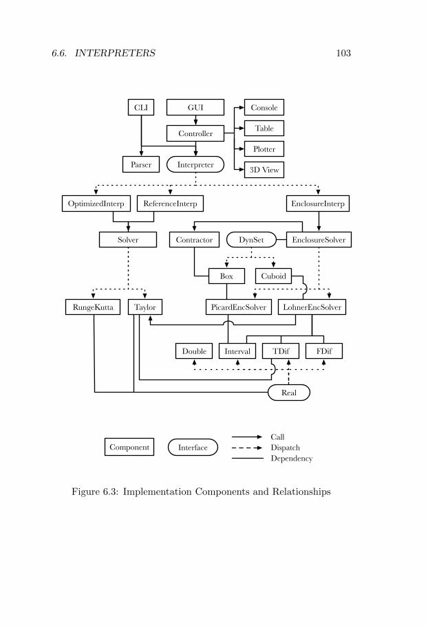
6.6. INTERPRETERS 103
GUI
EnclosureInterpOptimizedInterp ReferenceInterp
Real
Double Interval TDif FDif
Solver EnclosureSolver
PicardEncSolver LohnerEncSolverRungeKutta Taylor
CuboidBox
Interpreter
DynSetContractor
Controller Table
3D View
ConsoleCLI
Parser
Plotter
Component InterfaceCallDispatchDependency
Figure 6.3: Implementation Components and Relationships
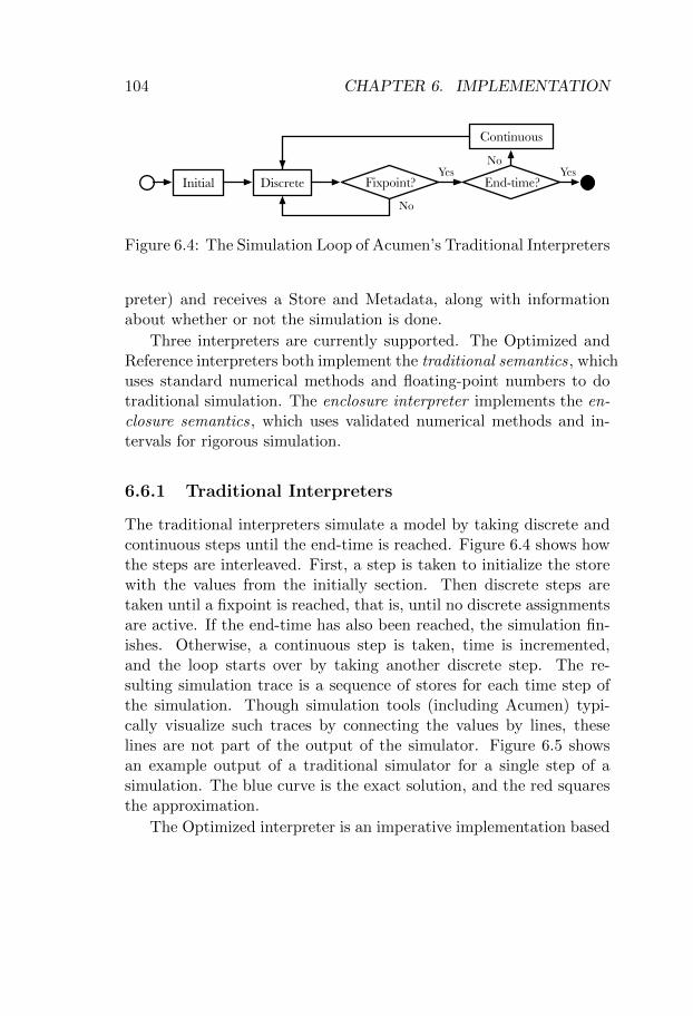
104 CHAPTER 6. IMPLEMENTATION
Initial Discrete
Continuous
Fixpoint? End-time?Yes Yes
No
No
Figure 6.4: The Simulation Loop of Acumen’s Traditional Interpreters
preter) and receives a Store and Metadata, along with informationabout whether or not the simulation is done.
Three interpreters are currently supported. The Optimized andReference interpreters both implement the traditional semantics, whichuses standard numerical methods and floating-point numbers to dotraditional simulation. The enclosure interpreter implements the en-closure semantics, which uses validated numerical methods and in-tervals for rigorous simulation.
6.6.1 Traditional Interpreters
The traditional interpreters simulate a model by taking discrete andcontinuous steps until the end-time is reached. Figure 6.4 shows howthe steps are interleaved. First, a step is taken to initialize the storewith the values from the initially section. Then discrete steps aretaken until a fixpoint is reached, that is, until no discrete assignmentsare active. If the end-time has also been reached, the simulation fin-ishes. Otherwise, a continuous step is taken, time is incremented,and the loop starts over by taking another discrete step. The re-sulting simulation trace is a sequence of stores for each time step ofthe simulation. Though simulation tools (including Acumen) typi-cally visualize such traces by connecting the values by lines, theselines are not part of the output of the simulator. Figure 6.5 showsan example output of a traditional simulator for a single step of asimulation. The blue curve is the exact solution, and the red squaresthe approximation.
The Optimized interpreter is an imperative implementation based
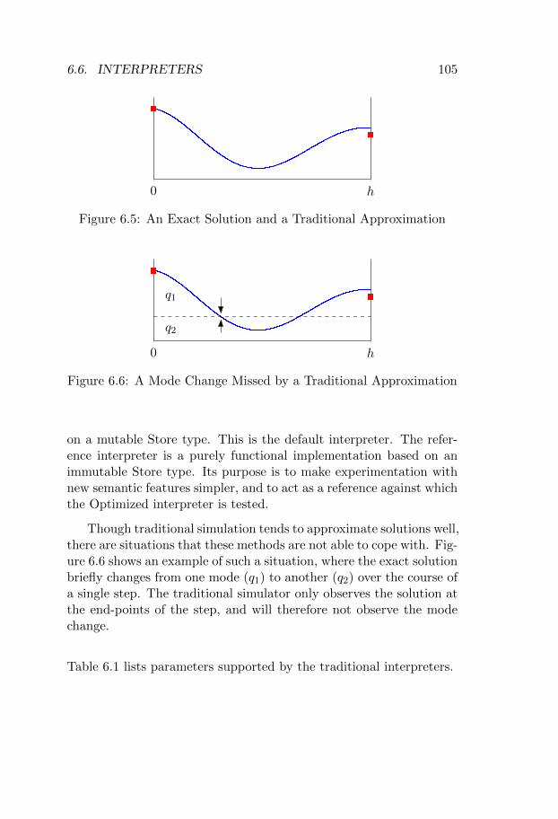
6.6. INTERPRETERS 105
0 h
Figure 6.5: An Exact Solution and a Traditional Approximation
0 h
q1
q2
Figure 6.6: A Mode Change Missed by a Traditional Approximation
on a mutable Store type. This is the default interpreter. The refer-ence interpreter is a purely functional implementation based on animmutable Store type. Its purpose is to make experimentation withnew semantic features simpler, and to act as a reference against whichthe Optimized interpreter is tested.
Though traditional simulation tends to approximate solutions well,there are situations that these methods are not able to cope with. Fig-ure 6.6 shows an example of such a situation, where the exact solutionbriefly changes from one mode (q1) to another (q2) over the course ofa single step. The traditional simulator only observes the solution atthe end-points of the step, and will therefore not observe the modechange.
Table 6.1 lists parameters supported by the traditional interpreters.
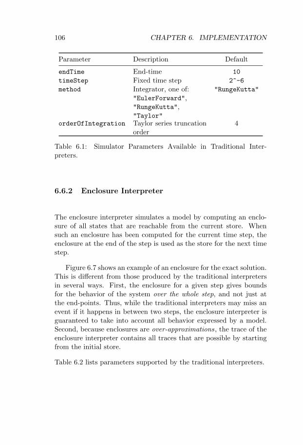
106 CHAPTER 6. IMPLEMENTATION
Parameter Description Default
endTime End-time 10
timeStep Fixed time step 2^-6
method Integrator, one of:"EulerForward","RungeKutta","Taylor"
"RungeKutta"
orderOfIntegration Taylor series truncationorder
4
Table 6.1: Simulator Parameters Available in Traditional Inter-preters.
6.6.2 Enclosure Interpreter
The enclosure interpreter simulates a model by computing an enclo-sure of all states that are reachable from the current store. Whensuch an enclosure has been computed for the current time step, theenclosure at the end of the step is used as the store for the next timestep.
Figure 6.7 shows an example of an enclosure for the exact solution.This is different from those produced by the traditional interpretersin several ways. First, the enclosure for a given step gives boundsfor the behavior of the system over the whole step, and not just atthe end-points. Thus, while the traditional interpreters may miss anevent if it happens in between two steps, the enclosure interpreter isguaranteed to take into account all behavior expressed by a model.Second, because enclosures are over-approximations, the trace of theenclosure interpreter contains all traces that are possible by startingfrom the initial store.
Table 6.2 lists parameters supported by the traditional interpreters.
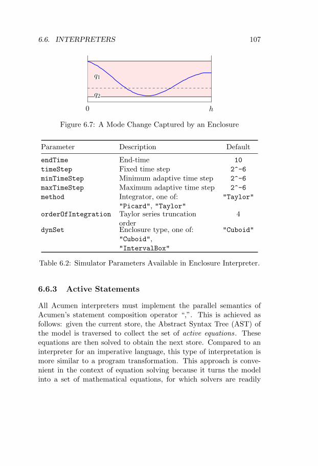
6.6. INTERPRETERS 107
0 h
q1q1
q2q2
Figure 6.7: A Mode Change Captured by an Enclosure
Parameter Description Default
endTime End-time 10
timeStep Fixed time step 2^-6
minTimeStep Minimum adaptive time step 2^-6
maxTimeStep Maximum adaptive time step 2^-6
method Integrator, one of:"Picard", "Taylor"
"Taylor"
orderOfIntegration Taylor series truncationorder
4
dynSet Enclosure type, one of:"Cuboid","IntervalBox"
"Cuboid"
Table 6.2: Simulator Parameters Available in Enclosure Interpreter.
6.6.3 Active Statements
All Acumen interpreters must implement the parallel semantics ofAcumen’s statement composition operator “,”. This is achieved asfollows: given the current store, the Abstract Syntax Tree (AST) ofthe model is traversed to collect the set of active equations. Theseequations are then solved to obtain the next store. Compared to aninterpreter for an imperative language, this type of interpretation ismore similar to a program transformation. This approach is conve-nient in the context of equation solving because it turns the modelinto a set of mathematical equations, for which solvers are readily
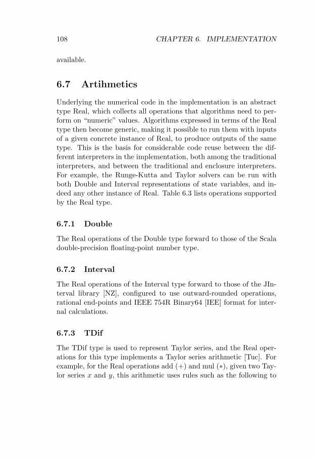
108 CHAPTER 6. IMPLEMENTATION
available.
6.7 Artihmetics
Underlying the numerical code in the implementation is an abstracttype Real, which collects all operations that algorithms need to per-form on “numeric” values. Algorithms expressed in terms of the Realtype then become generic, making it possible to run them with inputsof a given concrete instance of Real, to produce outputs of the sametype. This is the basis for considerable code reuse between the dif-ferent interpreters in the implementation, both among the traditionalinterpreters, and between the traditional and enclosure interpreters.For example, the Runge-Kutta and Taylor solvers can be run withboth Double and Interval representations of state variables, and in-deed any other instance of Real. Table 6.3 lists operations supportedby the Real type.
6.7.1 Double
The Real operations of the Double type forward to those of the Scaladouble-precision floating-point number type.
6.7.2 Interval
The Real operations of the Interval type forward to those of the JIn-terval library [NZ], configured to use outward-rounded operations,rational end-points and IEEE 754R Binary64 [IEE] format for inter-nal calculations.
6.7.3 TDif
The TDif type is used to represent Taylor series, and the Real oper-ations for this type implements a Taylor series arithmetic [Tuc]. Forexample, for the Real operations add (+) and mul (∗), given two Tay-lor series x and y, this arithmetic uses rules such as the following to
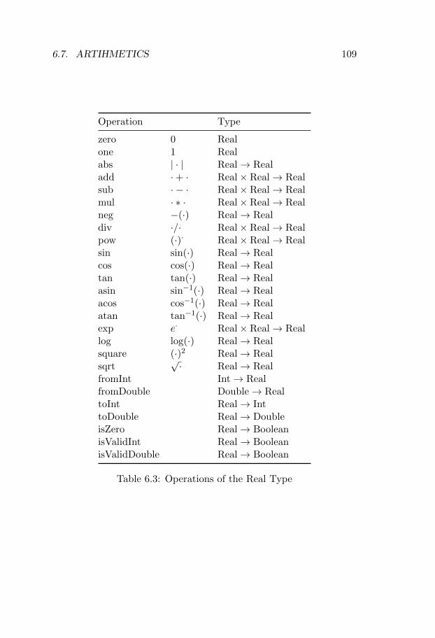
6.7. ARTIHMETICS 109
Operation Type
zero 0 Realone 1 Realabs | · | Real→ Realadd ·+ · Real× Real→ Realsub · − · Real× Real→ Realmul · ∗ · Real× Real→ Realneg −(·) Real→ Realdiv ·/· Real× Real→ Realpow (·)· Real× Real→ Realsin sin(·) Real→ Realcos cos(·) Real→ Realtan tan(·) Real→ Realasin sin−1(·) Real→ Realacos cos−1(·) Real→ Realatan tan−1(·) Real→ Realexp e· Real× Real→ Reallog log(·) Real→ Realsquare (·)2 Real→ Realsqrt
√· Real→ Real
fromInt Int→ RealfromDouble Double→ RealtoInt Real→ InttoDouble Real→ DoubleisZero Real→ BooleanisValidInt Real→ BooleanisValidDouble Real→ Boolean
Table 6.3: Operations of the Real Type
110 CHAPTER 6. IMPLEMENTATION
compute the coefficient of the k:th term of the combined series:
(x+ y)k = xk + yk(x ∗ y)k =
∑ki=0 xiyk−i
6.7.4 FDif
The FDif type is used to represent gradients. In the context of Acu-men, a gradient is the value of a variable together with its partialderivatives, with respect to all other variables in a model. The Realoperations for this type implement a gradient arithmetic [Ral]. Forexample, for the Real operations add (+) and mul (∗), given twogradients x and y, this arithmetic uses rules such as the following tocompute the components of the combined gradient:
(x+ y)k = xk + yk
(x ∗ y)k =
{x0y0 if k = 0
x0yk + y0xk otherwise
Here, the 0:th component contains the value of the variable itself.
6.8 Solvers
The traditional interpreters can use one of two integrators to solvedifferential equations: Runge-Kutta and Taylor. Both of them areimplemented in terms of the Real numeric type (Section 6.7), andcan thus be evaluated using any of its subtypes.
6.8.1 Runge-Kutta
The Runge-Kutta solver implements a fourth-order Runge-Kutta in-tegrator that behaves well for many models, and is computationallyefficient. It is the default solver for the traditional interpreters.
6.8. SOLVERS 111
6.8.2 Taylor
The Taylor solver implements a (truncated) Taylor series integrator.Because the Taylor series can be chosen to be of any order, this inte-grator can be used to solve highly non-linear equations, such as thoseused to describe the motion of a double pendulum, whose solutionsmay become unstable with the default integrator.
The enclosure interpreter makes use of two rigorous ODE IVP solversand an interval box contractor [CJ].
6.8.3 Picard
The Picard solver implements a first-order polynomial function inter-val Picard integrator [KDFT]. It is based on a variant of the Picarditerator :
x(t) = x(0) +
∫ t
s=0f(s, x(s))ds (6.1)
where the solution x(t) at each iteration is represented by a functioninterval [DFKT], that is, a pair of functions (the upper and lowerbounds). Though the current implementation of this solver is lim-ited by its first-order polynomial enclosure type, it can (in principle)be used to solve any ODE IVP whose field is Lipschitz continuous.Notably, this includes ODEs, whose fields are not differentiable.
6.8.4 Lohner
The Lohner solver implements a validated Taylor series integrator[Loh; Ned; Bar]. This solver is suitable for solving non-linear ODEIVPs and uses the Cuboid enclosure (DynSet) type as its input andoutput. A Cuboid represents the continuous state of a model as aparallelepiped, that is, as follows:
midpoint + linearTransform ∗ width + error (6.2)
where midpoint, width, and error are Real vectors and linearTrans-form is a Real matrix. When the solver is initialized, the initial
112 CHAPTER 6. IMPLEMENTATION
condition is represented in centered form as midpoint and width. ThelinearTransform is initialized to an identity matrix, and error is ini-tialized to a null vector. Basically, the solver integrates an ODE byupdating the linearTransform matrix and multiplying it by the Jaco-bian of the solution approximation at each step, to capture the effectthat the ODE exerts on the initial condition.
Both the TDif and FDif types are parameterized by another Realtype that represents their coefficients (TDif) and components (FDif).This ability to nest Real types is crucial for the implementation ofthis solver, where the computation of the Jacobian of the solutionmap involves a call to the Taylor solver that combines Interval, TDifand FDif arithmetics.
6.8.5 Contractor
The Contractor implements the HC4Revise [ILO] interval box con-tractor. Given an interval box (multidimensional interval) x : Rn anda constraint4 C : Rn → B this algorithm produces an interval box ythat satisfies the following two properties for any z ⊆ Rn:
• C(x) ⊆ x
• C(x) ∩ z = x ∩ z
In the implementation, the interval box is a value of the Box typeand the constraint a set of Boolean expressions.
6.8.6 Plotter and Table
The Plotter and Table components provide direct views of the dataproduced by the interpreter. The Table displays data for each simula-tion step as a row whose columns are variable names. Value producedby the enclosure interpreter are displayed either as sets of values (for
4 The implementation of the Contractor is limited compared to the other vali-dated solvers, and is currently missing some non-linear functions, such as sin andcos.
6.9. TESTING 113
string or Boolean variables) or as intervals (for real variables). ThePlotter component displays simulation steps differently depending onthe interpreter that produced them. Data for steps produced by thetraditional interpreters are plotted as points connected by lines. Datafor steps produced by the enclosure interpreter are plotted in one oftwo ways. Discrete (string and Boolean) variables are plotted as setsof points. Points at consecutive time steps that correspond to thesame discrete value are connected by lines. Real variables are plottedas intervals.
6.8.7 3D View
The 3D View component [Zen] visualizes 3D models embedded in anAcumen model. By visualizing the simulation result in a form thatclosely matches the modeled system, it provides a way to quicklyunderstand overall system behavior. For example, the 3D visualiza-tion proved invaluable in debugging the model of the automotive casestudy (Chapter 7), where a large number of variables interact to pro-duce events such as a collision.
3D models are built from built-in geometric primitives, or from3D meshes created in a third-party tool such as Blender [Ble]. The3D visualization is animated by using variables from the dynamicalmodel in the 3D model. The animation can be displayed in real timeduring a simulation, and the user can interact with the simulationusing an input device [Xu].
6.9 Testing
Given the complexity of Acumen, and its objective to be rigorous,automated testing has been an important aspect of its development.The automated tests can be divided into two categories.
The first kind are unit tests, which check individual test cases.The basic unit tests check the correct behavior of a function for aparticular input. Such tests are useful to detect regressions, thatis, changes to the code base that break existing functionality. For
114 CHAPTER 6. IMPLEMENTATION
example, when a bug has been fixed, a unit test marked with anidentifier for that bug is added to the code base to make the testsuite fail if a subsequent change re-introduces the bug. Acumen’stest suite also includes regression tests that check the behavior of theinterpreters on example models from the distribution. The output iscompared to previously generated reference output files. These testsare useful to detect accidental, semantics-altering changes.
The second kind are generator-driven property-based tests [CH;TGP; Sca]. In such tests, the property is specified as a Booleanexpression in terms of the tested function. The the test cases arethen generated based on the types of the expression’s free variables.Property-based tests are used extensively in the implementation tocheck basic properties of the arithmetics. For example, the imple-mentation contains tests of trigonometric identities such as −1 ≤ x ≤1 =⇒ x = sin(asin(x)). Equalities do not generally hold whenworking with approximations, so these tests typically use an approxi-mate equality operator. This introduces the problem of choosing howclose two values must be to be considered equal. This problem canbe avoided when testing operations based on validated numerics, byreplacing equality with subset inclusion or intersection. For exam-ple, the above equation can be replaced by: x ⊆ sin(asin(x)). Thisweakens the test – an implementation of sin that returns the con-stant [−1 .. 1] satisfies the new property – but combined with othertests these properties have still helped us uncover bugs and increaseconfidence in the implementation.
The soundness criteria given in Definition 5.7.6 are further exam-ples of properties. Though such tests have not yet been added tothe implementation, they could serve as the basis of a test suite forexternal implementations of the validated numerical primitives.
Chapter 7
An Automotive CollisionCase Study1
Formal methods can provide guaranteed answers to questions in thepresence of uncertainty. This makes them interesting in the designof safety-critical systems where unaccounted error, be it from model-ing or from computation, can have dire consequences. Verification ofsafety-critical systems typically aims to establish that a certain safetyproperty holds. In the case of air traffic control, such a property couldbe that the trajectories of two airplanes remain at a safe distance fromone another, that an evasive maneuver is enacted if the distance fallsbelow some threshold, and that the maneuver successfully maintainsthe safe distance. Due to the controlled nature of avionics and the
1This chapter consolidates and extends several results presented at FISITA2014 [MPD+] and ICESS 2015 [DEB+]. The first version investigated the fea-sibility of using rigorous simulators in the automotive domain, using a simpleone-dimensional model expressed as a single hybrid automaton. The second pa-per reported on a simulator capable of executing two-dimensional scenarios, withcollision and sensor models based on rectangular vehicles and a braking controllerbased on time-to-collision. The present version adds a significantly improvedmodel, including a combination of multiple braking criteria based on recommenda-tions from the automotive industry, and a more precise model of the sensor range(trapezoid). Sections 7.3 to 7.6 and were added to explain the improved model indetail.
115
116 CHAPTER 7. AUTOMOTIVE CASE STUDY
high risks involved in it, significant effort has gone into the verificationof air traffic control systems [PC; JM]. With the recent introductionof autonomy features in road vehicles, formal verification of these con-trol systems is becoming increasingly important. Recent work on theverification of such systems includes a safety proof of a distributedautomotive traffic control algorithm [LPN] and computing the prob-ability of a crash [A+1]. In this chapter we will look at how rigoroussimulation can be used to perform a related task – to compute boundson a quantity estimated by a model. The result is used in a safetyanalysis to assess the danger of a given simulated scenario.
7.1 Hazard Analysis And Risk Assessmentand The ISO 26262 Standard
To address the need for automotive system safety guidelines and reg-ulations, the industry has developed the ISO 26262 standard [ISO]. Itformalizes safety in (passenger) road vehicles, including requirementsfor the design of control systems and notions, based on which thesafety of such systems can be evaluated. To comply with the stan-dard, a system must undergo a Hazard Analysis and Risk Assessment(HARA).
In risk assessment terminology, a hazard is a possible source ofharm and risk is the probability of this harm. Risk is further brokendown as a combination of severity, exposure, and likelihood. Severityis a measure of the injury that follows from harm. Exposure is theexpected frequency of the conditions under which the injury can oc-cur. Likelihood is the probability that the harm will occur given theexposure.
Traffic hazards include sudden lane changes, slippery roads, andintersections. The harm associated with these hazards is injury due toa collision. We can break down the associated risk into the seriousnessof the injury (severity), the proportion of time that drivers spendcrossing intersections (exposure) and the probability that a collisionwill take place when crossing the intersection (likelihood).
Mirroring standards from other safety-critical domains, ISO 26262
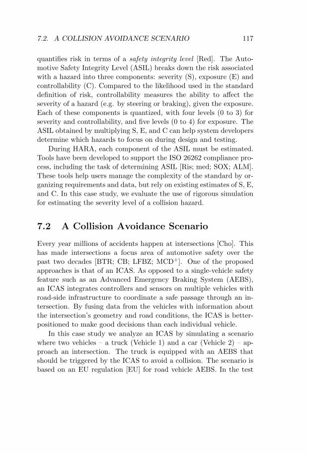
7.2. A COLLISION AVOIDANCE SCENARIO 117
quantifies risk in terms of a safety integrity level [Red]. The Auto-motive Safety Integrity Level (ASIL) breaks down the risk associatedwith a hazard into three components: severity (S), exposure (E) andcontrollability (C). Compared to the likelihood used in the standarddefinition of risk, controllability measures the ability to affect theseverity of a hazard (e.g. by steering or braking), given the exposure.Each of these components is quantized, with four levels (0 to 3) forseverity and controllability, and five levels (0 to 4) for exposure. TheASIL obtained by multiplying S, E, and C can help system developersdetermine which hazards to focus on during design and testing.
During HARA, each component of the ASIL must be estimated.Tools have been developed to support the ISO 26262 compliance pro-cess, including the task of determining ASIL [Ris; med; SOX; ALM].These tools help users manage the complexity of the standard by or-ganizing requirements and data, but rely on existing estimates of S, E,and C. In this case study, we evaluate the use of rigorous simulationfor estimating the severity level of a collision hazard.
7.2 A Collision Avoidance Scenario
Every year millions of accidents happen at intersections [Cho]. Thishas made intersections a focus area of automotive safety over thepast two decades [BTR; CB; LFBZ; MCD+]. One of the proposedapproaches is that of an ICAS. As opposed to a single-vehicle safetyfeature such as an Advanced Emergency Braking System (AEBS),an ICAS integrates controllers and sensors on multiple vehicles withroad-side infrastructure to coordinate a safe passage through an in-tersection. By fusing data from the vehicles with information aboutthe intersection’s geometry and road conditions, the ICAS is better-positioned to make good decisions than each individual vehicle.
In this case study we analyze an ICAS by simulating a scenariowhere two vehicles – a truck (Vehicle 1) and a car (Vehicle 2) – ap-proach an intersection. The truck is equipped with an AEBS thatshould be triggered by the ICAS to avoid a collision. The scenario isbased on an EU regulation [EU] for road vehicle AEBS. In the test
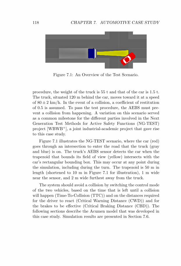
118 CHAPTER 7. AUTOMOTIVE CASE STUDY
Figure 7.1: An Overview of the Test Scenario.
procedure, the weight of the truck is 55 t and that of the car is 1.5 t.The truck, situated 120 m behind the car, moves toward it at a speedof 80± 2 km/h. In the event of a collision, a coefficient of restitutionof 0.5 is assumed. To pass the test procedure, the AEBS must pre-vent a collision from happening. A variation on this scenario servedas a common milestone for the different parties involved in the NextGeneration Test Methods for Active Safety Functions (NG-TEST)project [WBWB+], a joint industrial-academic project that gave riseto this case study.
Figure 7.1 illustrates the NG-TEST scenario, where the car (red)goes through an intersection to enter the road that the truck (grayand blue) is on. The truck’s AEBS sensor detects the car when thetrapezoid that bounds its field of view (yellow) intersects with thecar’s rectangular bounding box. This may occur at any point duringthe simulation, including during the turn. The trapezoid is 50 m inlength (shortened to 10 m in Figure 7.1 for illustration), 1 m widenear the sensor, and 2 m wide furthest away from the truck.
The system should avoid a collision by switching the control modeof the two vehicles, based on the time that is left until a collisionwill happen (Time-To-Collision (TTC)) and on the distances requiredfor the driver to react (Critical Warning Distance (CWD)) and forthe brakes to be effective (Critical Braking Distance (CBD)). Thefollowing sections describe the Acumen model that was developed inthis case study. Simulation results are presented in Section 7.6.
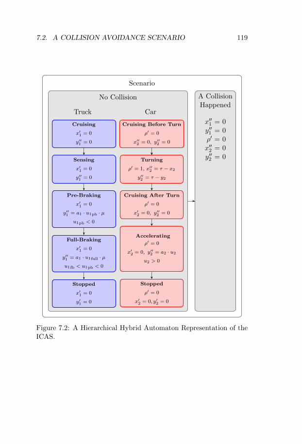
7.2. A COLLISION AVOIDANCE SCENARIO 119
Scenario
No Collision
Truck
Cruising
x′1 = 0
y′′1 = 0
Sensing
x′1 = 0
y′′1 = 0
Pre-Braking
x′1 = 0
y′′1 = a1 · u1pb · µu1pb < 0
Full-Braking
x′1 = 0
y′′1 = a1 · u1full · µu1fb < u1pb < 0
Stopped
x′1 = 0
y′1 = 0
Car
Cruising Before Turn
ρ′ = 0
x′′2 = 0, y′′2 = 0
Turning
ρ′ = 1, x′′2 = τ − x2y′′2 = τ − y2
Cruising After Turn
ρ′ = 0
x′2 = 0, y′′2 = 0
Accelerating
ρ′ = 0
x′2 = 0, y′′2 = a2 · u2u2 > 0
Stopped
ρ′ = 0
x′2 = 0, y′2 = 0
A CollisionHappened
x′′1 = 0y′′1 = 0ρ′ = 0x′′2 = 0y′′2 = 0
Figure 7.2: A Hierarchical Hybrid Automaton Representation of theICAS.
120 CHAPTER 7. AUTOMOTIVE CASE STUDY
7.3 Vehicle and Collision Models
Unlike sensor-based collision avoidance systems [BMAHA] such asAutomatic Emergency Braking [CEB], where a single vehicle actsautonomously to avoid a collision, ICA systems are a cooperative ap-proach to vehicle safety. Infrastructure located in the intersectioncoordinates two or more vehicles based on position and sensor datafrom the vehicles, as well as knowledge about the geometry of theintersection. Section 7.4 describes the Acumen model of the collisiondetection and avoidance system, including the two vehicles. Figure 7.2gives an overview of the model as a partial, nested hybrid automa-ton, where the controllers for the two vehicles are nested inside anautomaton that handles the collision.
7.4 Vehicle Dynamics (Pre-Collision)
Each vehicle is modeled as a two-dimensional point mass, as well as a(possibly rotated) bounding rectangle. The controller for each vehicleis modeled as a match statement that roughly corresponds to a hybridautomaton. The modes of this automaton correspond to the cases ofthe match, that is, the values of two variables: state1 for the truck;state2 for the car. Figure 7.2 illustrates the continuous dynamicsand key state variables that comprise the model. For space reasons,guard conditions and reset maps have been left out of the diagram.In the top-level “No Collision” mode, the dynamics of each vehicleare controlled by a separate automaton. Initial parameters passed tothe Scenario sub-model determine the initial positions and velocitiesfor the two vehicles, as well as the braking/acceleration applied whenthe car enters its “Accelerating” mode.
Truck
The dynamics of the truck are defined by a hybrid controller thatvaries the truck’s acceleration along the main road. Depending on howclose the vehicles are to a collision, the truck’s controller enters one of
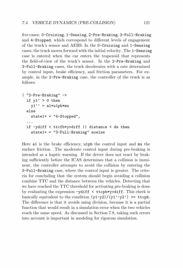
7.4. VEHICLE DYNAMICS (PRE-COLLISION) 121
five cases: 0-Cruising, 1-Sensing, 2-Pre-Braking, 3-Full-Brakingand 4-Stopped, which correspond to different levels of engagementof the truck’s sensor and AEBS. In the 0-Cruising and 1-Sensing
cases, the truck moves forward with the initial velocity. The 1-Sensingcase is entered when the car enters the trapezoid that representsthe field-of-view of the truck’s sensor. In the 2-Pre-Braking and3-Full-Braking cases, the truck decelerates with a rate determinedby control input, brake efficiency, and friction parameters. For ex-ample, in the 2-Pre-Braking case, the controller of the truck is asfollows:
| "2-Pre-Braking" ->
if y1’ > 0 then
y1’’ = a1*u1pb*mu
else
state1+ = "4-Stopped",
...
if -ydiff < ttcfb*yvdiff || distance < ds then
state1+ = "3-Full-Braking" noelse
Here a1 is the brake efficiency, u1pb the control input and mu thesurface friction. The moderate control input during pre-braking isintended as a haptic warning. If the driver does not react by brak-ing sufficiently before the ICAS determines that a collision is immi-nent, the controller attempts to avoid the collision by entering the3-Full-Braking case, where the control input is greater. The crite-ria for concluding that the system should begin avoiding a collisioncombine TTC and the distance between the vehicles. Detecting thatwe have reached the TTC threshold for activating pre-braking is doneby evaluating the expression -ydiff < ttcpb*yvdiff. This check isbasically equivalent to the condition (y1-y2)/(y1’-y2’) >= ttcpb.The difference is that it avoids using division, because it is a partialfunction that would result in a simulation error when the two vehiclesreach the same speed. As discussed in Section 7.8, taking such errorsinto account is important in modeling for rigorous simulation.
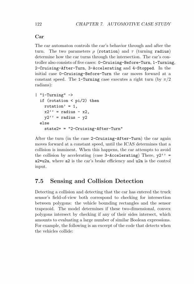
122 CHAPTER 7. AUTOMOTIVE CASE STUDY
Car
The car automaton controls the car’s behavior through and after theturn. The two parameters ρ (rotation) and τ (turning radius)determine how the car turns through the intersection. The car’s con-troller also consists of five cases: 0-Cruising-Before-Turn, 1-Turning,2-Cruising-After-Turn, 3-Accelerating and 4-Stopped. In theinitial case 0-Cruising-Before-Turn the car moves forward at aconstant speed. The 1-Turning case executes a right turn (by π/2radians):
| "1-Turning" ->
if (rotation < pi/2) then
rotation’ = 1,
x2’’ = radius - x2,
y2’’ = radius - y2
else
state2+ = "2-Cruising-After-Turn"
After the turn (in the case 2-Cruising-After-Turn) the car againmoves forward at a constant speed, until the ICAS determines that acollision is imminent. When this happens, the car attempts to avoidthe collision by accelerating (case 3-Accelerating) There, y2’’ =
a2*u2a, where a2 is the car’s brake efficiency and u2a is the controlinput.
7.5 Sensing and Collision Detection
Detecting a collision and detecting that the car has entered the trucksensor’s field-of-view both correspond to checking for intersectionbetween polygons: the vehicle bounding rectangles and the sensortrapezoid. The model determines if these two-dimensional, convexpolygons intersect by checking if any of their sides intersect, whichamounts to evaluating a large number of similar Boolean expressions.For example, the following is an excerpt of the code that detects whenthe vehicles collide:
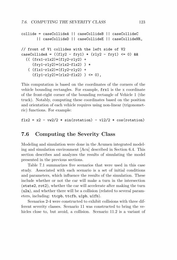
7.6. COMPUTING THE SEVERITY CLASS 123
collide = caseCollideA || caseCollideB || caseCollideC
|| caseCollideD || caseCollideE || caseCollideNR,
// front of V1 collides with the left side of V2
caseCollideA = ((fly2 - fry1) * (rly2 - fry1) <= 0) &&
(( (frx1-rlx2)*(fly2-rly2) +
(fry1-rly2)*(rlx2-flx2) ) *
( (flx1-rlx2)*(fly2-rly2) +
(fly1-rly2)*(rlx2-flx2) ) <= 0),
This computation is based on the coordinates of the corners of thevehicle bounding rectangles. For example, frx1 is the x coordinateof the front-right corner of the bounding rectangle of Vehicle 1 (thetruck). Notably, computing these coordinates based on the positionand orientation of each vehicle requires using non-linear (trigonomet-ric) functions. For example:
flx2 = x2 - vw2/2 * sin(rotation) - vl2/2 * cos(rotation)
7.6 Computing the Severity Class
Modeling and simulation were done in the Acumen integrated model-ing and simulation environment [Acu] described in Section 6.4. Thissection describes and analyzes the results of simulating the modelpresented in the previous sections.
Table 7.1 summarizes five scenarios that were used in this casestudy. Associated with each scenario is a set of initial conditionsand parameters, which influence the results of the simulation. Theseinclude whether or not the car will make a turn in the intersection(state2, rot2), whether the car will accelerate after making the turn(u2a), and whether there will be a collision (related to several param-eters, including: ttcpb, ttcfb, u1pb, u1fb).
Scenarios 2-4 were constructed to exhibit collisions with three dif-ferent severity classes. Scenario 11 was constructed to bring the ve-hicles close to, but avoid, a collision. Scenario 11.2 is a variant of
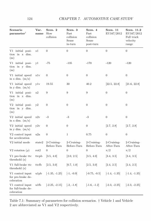
124 CHAPTER 7. AUTOMOTIVE CASE STUDY
Scenarioparameter†
Var.name
Scen. 2Slowcollision
Scen. 3FastcollisionSensein-turn
Scen. 4FastcollisionSensepost-turn
Scen. 11EU347/2012
Scen. 11.2EU347/2012Full truckvelocityrange
V1 initial posi-tion in x dim.(m)
x1 0 0 0 0 0
V1 initial posi-tion in y dim.(m)
y1 -75 -135 -170 -120 -120
V1 initial speedin x dim. (m/s)
x1v 0 0 0 0 0
V1 initial speedin y dim. (m/s)
y1v 19.55 30 40.2 [22.5, 22.8] [21.6, 22.8]
V1 initial posi-tion in x dim.(m)
x2 9 9 9 0 0
V2 initial posi-tion in y dim.(m)
y2 0 0 0 0 0
V2 initial speedin x dim. (m/s)
x2v -3 -3 -3 0 0
V2 initial speedin y dim. (m/s)
y2v 0 0 0 [2.7, 2.8] [2.7, 2.8]
V2 control inputfor acceleration
u2a 0 1 0.75 0 0
V2 initial mode state2 2-Cruising-Before-Turn
2-Cruising-Before-Turn
2-Cruising-Before-Turn
2-Cruising-After-Turn
2-Cruising-After-Turn
V2 rotation (ρ) rot2 0 0 0 π/2 π/2
V1 pre-brake ttcthreshold (s)
ttcpb [3.5, 4.0] [2.0, 2.5] [3.5, 4.0] [3.4, 3.5] [3.4, 3.5]
V1 full-brake ttcthreshold (s)
ttcfb [2.5, 3.0] [0.7, 1.0] [2.5, 3.0] [2.4, 2.5] [2.4, 2.5]
V1 control inputfor pre-brake de-celeration
u1pb [-1.35, -1.25] [-1, -0.9] [-0.75, -0.5] [-1.4, -1.35] [-1.4, -1.35]
V1 control inputfor full-brake de-celeration
u1fb [-2.25, -2.15] [-2, -1.8] [-1.6, -1.2] [-2.3, -2.25] [-2.3, -2.25]
Table 7.1: Summary of parameters for collision scenarios. † Vehicle 1 and Vehicle2 are abbreviated as V1 and V2 respectively.
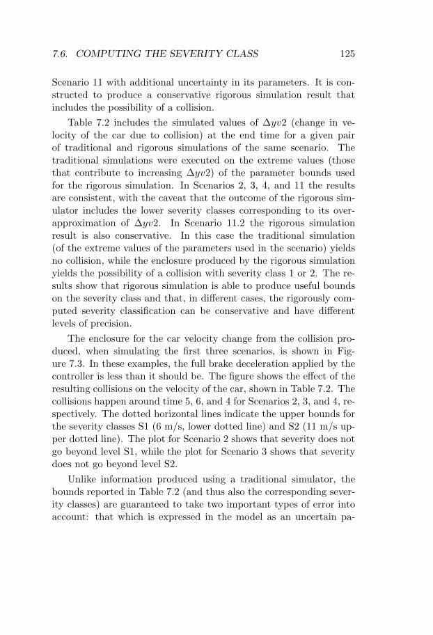
7.6. COMPUTING THE SEVERITY CLASS 125
Scenario 11 with additional uncertainty in its parameters. It is con-structed to produce a conservative rigorous simulation result thatincludes the possibility of a collision.
Table 7.2 includes the simulated values of ∆yv2 (change in ve-locity of the car due to collision) at the end time for a given pairof traditional and rigorous simulations of the same scenario. Thetraditional simulations were executed on the extreme values (thosethat contribute to increasing ∆yv2) of the parameter bounds usedfor the rigorous simulation. In Scenarios 2, 3, 4, and 11 the resultsare consistent, with the caveat that the outcome of the rigorous sim-ulator includes the lower severity classes corresponding to its over-approximation of ∆yv2. In Scenario 11.2 the rigorous simulationresult is also conservative. In this case the traditional simulation(of the extreme values of the parameters used in the scenario) yieldsno collision, while the enclosure produced by the rigorous simulationyields the possibility of a collision with severity class 1 or 2. The re-sults show that rigorous simulation is able to produce useful boundson the severity class and that, in different cases, the rigorously com-puted severity classification can be conservative and have differentlevels of precision.
The enclosure for the car velocity change from the collision pro-duced, when simulating the first three scenarios, is shown in Fig-ure 7.3. In these examples, the full brake deceleration applied by thecontroller is less than it should be. The figure shows the effect of theresulting collisions on the velocity of the car, shown in Table 7.2. Thecollisions happen around time 5, 6, and 4 for Scenarios 2, 3, and 4, re-spectively. The dotted horizontal lines indicate the upper bounds forthe severity classes S1 (6 m/s, lower dotted line) and S2 (11 m/s up-per dotted line). The plot for Scenario 2 shows that severity does notgo beyond level S1, while the plot for Scenario 3 shows that severitydoes not go beyond level S2.
Unlike information produced using a traditional simulator, thebounds reported in Table 7.2 (and thus also the corresponding sever-ity classes) are guaranteed to take two important types of error intoaccount: that which is expressed in the model as an uncertain pa-
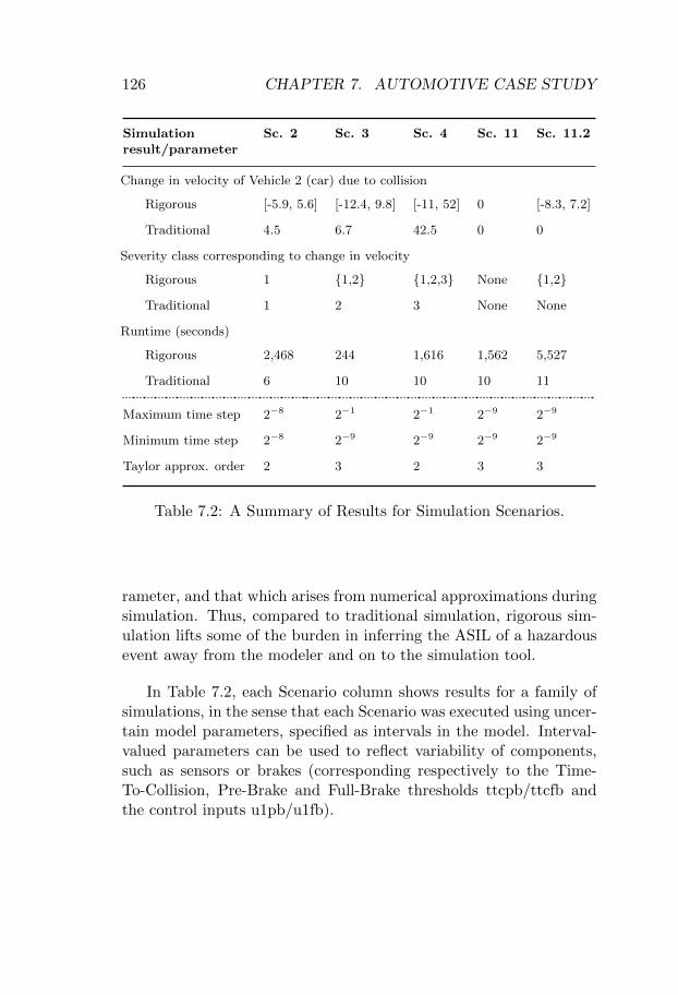
126 CHAPTER 7. AUTOMOTIVE CASE STUDY
Simulationresult/parameter
Sc. 2 Sc. 3 Sc. 4 Sc. 11 Sc. 11.2
Change in velocity of Vehicle 2 (car) due to collision
Rigorous [-5.9, 5.6] [-12.4, 9.8] [-11, 52] 0 [-8.3, 7.2]
Traditional 4.5 6.7 42.5 0 0
Severity class corresponding to change in velocity
Rigorous 1 {1,2} {1,2,3} None {1,2}
Traditional 1 2 3 None None
Runtime (seconds)
Rigorous 2,468 244 1,616 1,562 5,527
Traditional 6 10 10 10 11
Maximum time step 2−8 2−1 2−1 2−9 2−9
Minimum time step 2−8 2−9 2−9 2−9 2−9
Taylor approx. order 2 3 2 3 3
Table 7.2: A Summary of Results for Simulation Scenarios.
rameter, and that which arises from numerical approximations duringsimulation. Thus, compared to traditional simulation, rigorous sim-ulation lifts some of the burden in inferring the ASIL of a hazardousevent away from the modeler and on to the simulation tool.
In Table 7.2, each Scenario column shows results for a family ofsimulations, in the sense that each Scenario was executed using uncer-tain model parameters, specified as intervals in the model. Interval-valued parameters can be used to reflect variability of components,such as sensors or brakes (corresponding respectively to the Time-To-Collision, Pre-Brake and Full-Brake thresholds ttcpb/ttcfb andthe control inputs u1pb/u1fb).
7.7. LIMITATIONS 127
-100
-50
0
50
100
150
0 2 4 6 8 10
Truck
Car
-100
-50
0
50
100
150
0 2 4 6 8 10
Truck
Car
-100
-50
0
50
100
150
0 2 4 6 8 10
Truck
Car
∆in
vel
oci
tyP
osi
tion
alo
ngy
-10
0
10
20
30
40
50
0 2 4 6 8 10
Time
(a) Scenario 2
-10
0
10
20
30
40
50
0 2 4 6 8 10
Time
(b) Scenario 3
-10
0
10
20
30
40
50
0 2 4 6 8 10
Time
(c) Scenario 4
Figure 7.3: Enclosures for Vehicle Positions and Change in VelocityDue to Collision.
7.7 Limitations
Simulation with uncertain parameters makes it possible for a sin-gle simulation to consider a range of scenarios. Acumen’s currentrigorous simulator can simulate some models with uncertain initialstate (Chapter 8) but is sensitive to large uncertainties. When manyuncertainties are combined it may take much longer to complete asimulation, and the result may also be inconclusive. For example,the scenario described in the EU347/2012 regulation, represented byScenario 11 in our model, considers speeds of 80 ± 2 km/h for theinitial speed of the truck (y1v). Acumen is currently able to sim-ulate this scenario successfully, showing that no collision is possible.Introducing uncertainty into other variables simultaneously (Scenario
128 CHAPTER 7. AUTOMOTIVE CASE STUDY
11.2) leads to a simulation result that does not rule out the possibilityof a collision. This example illustrates the limits of what Acumen’srigorous simulator is currently capable of.
7.8 Remarks About our Experience Develop-ing the Model using Acumen
This section summarizes practical issues that arose during the processof modeling and rigorous simulation of this system
Acumen allows the user to run the same model using traditionaland rigorous simulation. The traditional simulation is faster and,in the case of an error in the model, it produces simpler error mes-sages. Thus, we found it convenient to use non-rigorous simulation todevelop the model in the first place, before switching to rigorous simu-lation. The latter currently takes significantly more time to complete,and the run-time properties of rigorous simulation are more sensitiveto the choice of simulation step. The ability to visualize the tra-ditional simulation results in 3D makes debugging efficient, and theintegration of the rigorous simulator with the 3D visualization facilityof Acumen is particularly important for enabling seamless alternationbetween non-rigorous and rigorous simulation, as the model is beingdeveloped. We now turn to the challenges that we encountered whenswitching between the traditional and rigorous simulators during ourwork on the model.
7.8.1 Avoiding Missed Events
The relatively complex geometry of the sensor field-of-view forced usto implement sensing using general intersection computations. Asthe shapes involved are convex polygons, we opted to check for inter-sections between the edges. This highlighted one of the benefits ofusing rigorous simulation. Namely, during the first edge intersectionin front/rear collisions (or sensing), the respective segments becomecollinear. Traditional simulation easily overlooks such scenarios, andthe user needs to implement additional, superfluous conditionals in
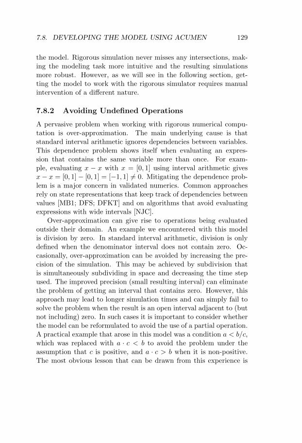
7.8. DEVELOPING THE MODEL USING ACUMEN 129
the model. Rigorous simulation never misses any intersections, mak-ing the modeling task more intuitive and the resulting simulationsmore robust. However, as we will see in the following section, get-ting the model to work with the rigorous simulator requires manualintervention of a different nature.
7.8.2 Avoiding Undefined Operations
A pervasive problem when working with rigorous numerical compu-tation is over-approximation. The main underlying cause is thatstandard interval arithmetic ignores dependencies between variables.This dependence problem shows itself when evaluating an expres-sion that contains the same variable more than once. For exam-ple, evaluating x − x with x = [0, 1] using interval arithmetic givesx− x = [0, 1]− [0, 1] = [−1, 1] 6= 0. Mitigating the dependence prob-lem is a major concern in validated numerics. Common approachesrely on state representations that keep track of dependencies betweenvalues [MB1; DFS; DFKT] and on algorithms that avoid evaluatingexpressions with wide intervals [NJC].
Over-approximation can give rise to operations being evaluatedoutside their domain. An example we encountered with this modelis division by zero. In standard interval arithmetic, division is onlydefined when the denominator interval does not contain zero. Oc-casionally, over-approximation can be avoided by increasing the pre-cision of the simulation. This may be achieved by subdivision thatis simultaneously subdividing in space and decreasing the time stepused. The improved precision (small resulting interval) can eliminatethe problem of getting an interval that contains zero. However, thisapproach may lead to longer simulation times and can simply fail tosolve the problem when the result is an open interval adjacent to (butnot including) zero. In such cases it is important to consider whetherthe model can be reformulated to avoid the use of a partial operation.A practical example that arose in this model was a condition a < b/c,which was replaced with a · c < b to avoid the problem under theassumption that c is positive, and a · c > b when it is non-positive.The most obvious lesson that can be drawn from this experience is
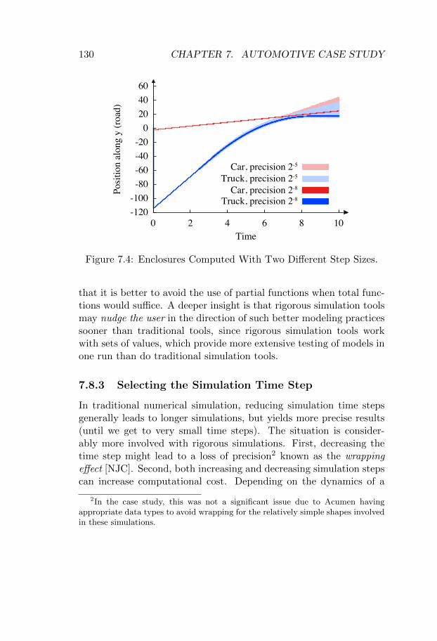
130 CHAPTER 7. AUTOMOTIVE CASE STUDY
Time
Car, precision 2-8
Car, precision 2-5
Truck, precision 2-8
Truck, precision 2-5
-120-100-80-60-40-200204060
0 2 4 6 8 10
Positionalongy(road)
Figure 7.4: Enclosures Computed With Two Different Step Sizes.
that it is better to avoid the use of partial functions when total func-tions would suffice. A deeper insight is that rigorous simulation toolsmay nudge the user in the direction of such better modeling practicessooner than traditional tools, since rigorous simulation tools workwith sets of values, which provide more extensive testing of models inone run than do traditional simulation tools.
7.8.3 Selecting the Simulation Time Step
In traditional numerical simulation, reducing simulation time stepsgenerally leads to longer simulations, but yields more precise results(until we get to very small time steps). The situation is consider-ably more involved with rigorous simulations. First, decreasing thetime step might lead to a loss of precision2 known as the wrappingeffect [NJC]. Second, both increasing and decreasing simulation stepscan increase computational cost. Depending on the dynamics of a
2In the case study, this was not a significant issue due to Acumen havingappropriate data types to avoid wrapping for the relatively simple shapes involvedin these simulations.
7.8. DEVELOPING THE MODEL USING ACUMEN 131
model, choosing a smaller step may help us obtain a conclusive out-come from a simulation. For example, one of the scenarios supportedby the model has the vehicles come close to collision but still avoidit. As shown in Figure 7.4, selecting a step that is too large (2−5,light colors) yields enclosures that include paths corresponding toa collision, which is insufficient to rule out the possibility of a col-lision. Decreasing the step by a factor of three (to 2−8, dark col-ors) shows conclusively that the collision does not occur. However,this does increase computational cost. Increasing simulation timesteps can also increase runtime. This happens because it can leadto greater uncertainty in the values of variables, which in turn canlead to more branching. Branching can happen when multiple timesteps are needed to determine conclusively that an enclosure crossesan event guard. During those steps, the simulator must branch thesimulation to take both cases into account (the event happening ornot happening in that step). It is possible that this problem is com-pounded if, before the branches can be recombined, they lead to morebranching. In such situations, decreasing the step can lead to a fastersimulation, by reducing the time spent on crossing event boundaries.
Acumen’s rigorous simulator can balance runtime and precisionby adapting the step size during the simulation. When different min-imum and maximum step sizes are provided by the user, the simulatorwill dynamically decrease the step size around time intervals wherethe dynamics change (such as when the control modes of the vehi-cles change, or at the collision), and increase the step size otherwise.Doing so can dramatically improve the runtime of a simulation. Forexample, the runtime of Scenario 3 is an order of magnitude fasterthan that of Scenario 2, even though the minimum time step used inScenario 2 is smaller. However, Acumen’s current adaptive steppingstrategy does incur a certain overhead, which may make the defaultfixed stepping preferable in some cases.

132 CHAPTER 7. AUTOMOTIVE CASE STUDY
Chapter 8
Benchmarks for theAccuracy of Enclosures1
This chapter reviews a collection of example models that can be usedas benchmarks to evaluate the accuracy of a rigorous simulator. Theexamples are models of stable systems, that is, models whose solutionsdo not diverge. Rigorous numerical computation, including rigoroussimulation, is sometimes criticized as being infeasible in practice, onaccount of an inevitable accumulation of numerical error. The col-lection of example models is used to empirically evaluate a designprinciple that addresses this criticism. The key insight underlyingthe principle is twofold:
1. Most man-made systems are designed to be stable and robustto variations in inputs and physical parameters.
2. Uncertainty due to approximation may be compensated by con-tracting dynamics.
These observations together suggest that the following principle isboth desirable and plausible:
1 This chapter is based on results presented at SNR 2016 [DBT]. Section 8.1.1has been extended with a discussion of the impact of the time step on over-approximation.
133
134 CHAPTER 8. ACCURACY
Accurate rigorous simulation should be possible for gooddesigns. In particular, enclosures computed by a rigoroussimulation tool for the trajectories of a robust and stablehybrid system should be converging.
This principle has been an important motivation for our own work,and we hope that it could be of value to others pursuing rigoroussimulation or similar methods.
In the rest of this chapter we present a suite of small, concretebenchmarks that can be used to assess the extent to which a rigoroussimulator upholds this principle. The benchmarks are classified intodiscrete and timed systems (Section 8.1); continuous systems (Sec-tion 8.2); and hybrid systems (Section 8.3). As the benchmarks arepresented, we identify those where Acumen’s current rigorous simu-lator [aR] already succeeds, and those where challenges still remain.Table 8.1 summarizes the results.
For the purposes of this chapter, we will view an enclosure as con-verging if it reaches a fixed point where it is a subset of the enclosure ata previous point in simulation time. For simplicity of implementation,we will further approximate this condition by testing set containmentonly in the enclosure of the simulation step that immediately precedesit.
8.1 Discrete and Timed Systems
This section presents examples of discrete systems where enclosuresshould converge, despite the presence of considerable uncertainty, notonly from numerical calculations but also from potential variabilityin system parameters.
8.1.1 Iteration and Nested Loops
Iteration can be expressed naturally in Acumen. For example, thecomputation for factorial of 5 can be expressed as follows:
model Disc1 () =
8.1. DISCRETE AND TIMED SYSTEMS 135
initially
n = 5, a = 1
always
if n > 0 then n+ = n-1, a+ = a*n noelse
A more interesting nested loop can be expressed as follows:
model Disc2 () =
initially i = 1, i_max = 3,
j = 1, j_max = 4,
k = 1, k_max = 5,
a = 0
always
if i<=i_max then
if j<=j_max then
if k<=k_max then
a+ = a+1, k+ = k+1
else (j+ = j+1, k+ = 1)
else (i+ = i+1, j+ = 1)
noelse
This example simply counts the number of iterations into the variablea. Because the computations are discrete (no integration, only rep-resentable numbers), Acumen computes a thin (that is, single value)enclosure for the result.
Even in models that abstract from continuous dynamics, we oftenwant to model computations as taking some time to compute. Thiscan be achieved using a clock variable to produce the following model:
model Disc3 () =
initially i = 1, i_max = 3,
j = 1, j_max = 4,
k = 1, k_max = 5,
a = 0, t = 0, t’ = 1
always
if t>0.1 then
t+ = 0,
136 CHAPTER 8. ACCURACY
if i<=i_max then
if j<=j_max then
if k<=k_max then
a+ = a+1, k+ = k+1
else (j+ = j+1, k+ = 1)
else (i+ = i+1, j+ = 1)
noelse
else t’= 1
Section 6.4 describes Acumen’s standard plot and how to read it.To read the plots included in this chapter, the reader should be awareof the following conventions:
• For diverging enclosures, the simulation is stopped at an ear-lier time than the default (10) to provide a more informativevisualization. In such cases, the time at which the simulation isstopped is indicated in the text.
• All plots are generated using a fixed time step of 2−6 to makeit easy to observe error caused by the discretization of time.
The plot for the model above is as follows:
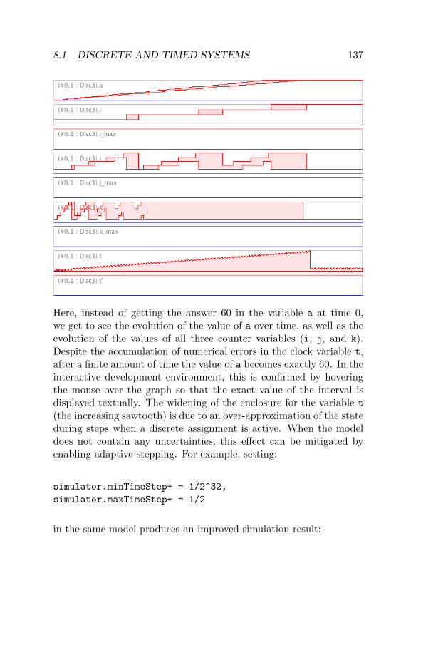
8.1. DISCRETE AND TIMED SYSTEMS 137
Here, instead of getting the answer 60 in the variable a at time 0,we get to see the evolution of the value of a over time, as well as theevolution of the values of all three counter variables (i, j, and k).Despite the accumulation of numerical errors in the clock variable t,after a finite amount of time the value of a becomes exactly 60. In theinteractive development environment, this is confirmed by hoveringthe mouse over the graph so that the exact value of the interval isdisplayed textually. The widening of the enclosure for the variable t
(the increasing sawtooth) is due to an over-approximation of the stateduring steps when a discrete assignment is active. When the modeldoes not contain any uncertainties, this effect can be mitigated byenabling adaptive stepping. For example, setting:
simulator.minTimeStep+ = 1/2^32,
simulator.maxTimeStep+ = 1/2
in the same model produces an improved simulation result:
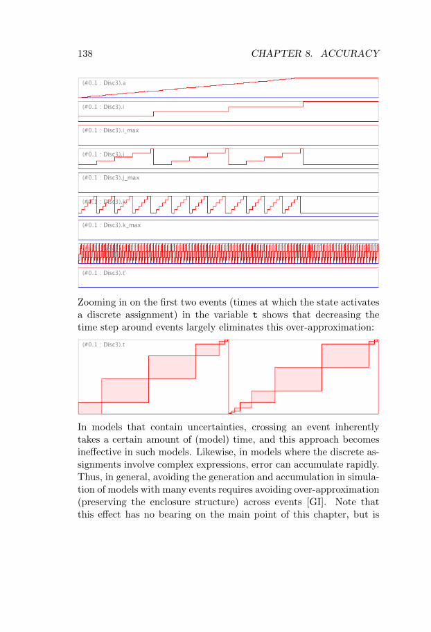
138 CHAPTER 8. ACCURACY
Zooming in on the first two events (times at which the state activatesa discrete assignment) in the variable t shows that decreasing thetime step around events largely eliminates this over-approximation:
In models that contain uncertainties, crossing an event inherentlytakes a certain amount of (model) time, and this approach becomesineffective in such models. Likewise, in models where the discrete as-signments involve complex expressions, error can accumulate rapidly.Thus, in general, avoiding the generation and accumulation in simula-tion of models with many events requires avoiding over-approximation(preserving the enclosure structure) across events [GI]. Note thatthis effect has no bearing on the main point of this chapter, but is
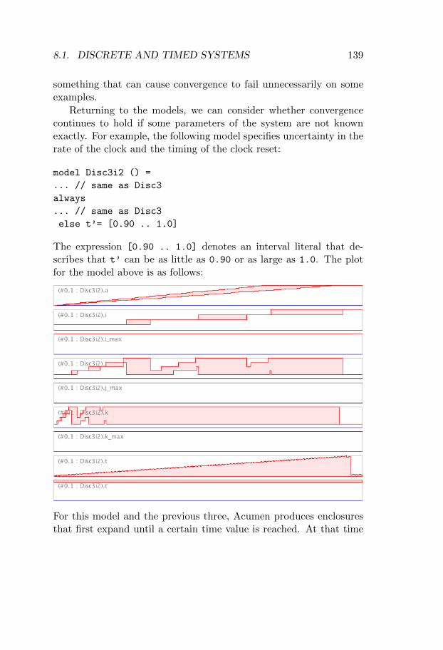
8.1. DISCRETE AND TIMED SYSTEMS 139
something that can cause convergence to fail unnecessarily on someexamples.
Returning to the models, we can consider whether convergencecontinues to hold if some parameters of the system are not knownexactly. For example, the following model specifies uncertainty in therate of the clock and the timing of the clock reset:
model Disc3i2 () =
... // same as Disc3
always
... // same as Disc3
else t’= [0.90 .. 1.0]
The expression [0.90 .. 1.0] denotes an interval literal that de-scribes that t’ can be as little as 0.90 or as large as 1.0. The plotfor the model above is as follows:
For this model and the previous three, Acumen produces enclosuresthat first expand until a certain time value is reached. At that time
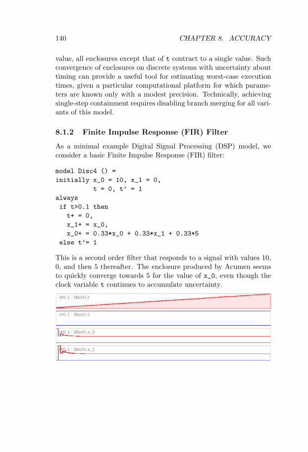
140 CHAPTER 8. ACCURACY
value, all enclosures except that of t contract to a single value. Suchconvergence of enclosures on discrete systems with uncertainty abouttiming can provide a useful tool for estimating worst-case executiontimes, given a particular computational platform for which parame-ters are known only with a modest precision. Technically, achievingsingle-step containment requires disabling branch merging for all vari-ants of this model.
8.1.2 Finite Impulse Response (FIR) Filter
As a minimal example Digital Signal Processing (DSP) model, weconsider a basic Finite Impulse Response (FIR) filter:
model Disc4 () =
initially x_0 = 10, x_1 = 0,
t = 0, t’ = 1
always
if t>0.1 then
t+ = 0,
x_1+ = x_0,
x_0+ = 0.33*x_0 + 0.33*x_1 + 0.33*5
else t’= 1
This is a second order filter that responds to a signal with values 10,0, and then 5 thereafter. The enclosure produced by Acumen seemsto quickly converge towards 5 for the value of x_0, even though theclock variable t continues to accumulate uncertainty.
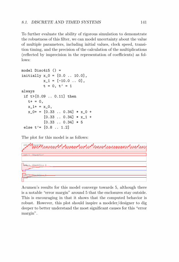
8.1. DISCRETE AND TIMED SYSTEMS 141
To further evaluate the ability of rigorous simulation to demonstratethe robustness of this filter, we can model uncertainty about the valueof multiple parameters, including initial values, clock speed, transi-tion timing, and the precision of the calculation of the multiplications(reflected by imprecision in the representation of coefficients) as fol-lows:
model Disc4i5 () =
initially x_0 = [0.0 .. 10.0],
x_1 = [-10.0 .. 0],
t = 0, t’ = 1
always
if t>[0.09 .. 0.11] then
t+ = 0,
x_1+ = x_0,
x_0+ = [0.33 .. 0.34] * x_0 +
[0.33 .. 0.34] * x_1 +
[0.33 .. 0.34] * 5
else t’= [0.8 .. 1.2]
The plot for this model is as follows:
Acumen’s results for this model converge towards 5, although thereis a notable “error margin” around 5 that the enclosures stay outside.This is encouraging in that it shows that the computed behavior isrobust. However, this plot should inspire a modeler/designer to digdeeper to better understand the most significant causes for this “errormargin”.
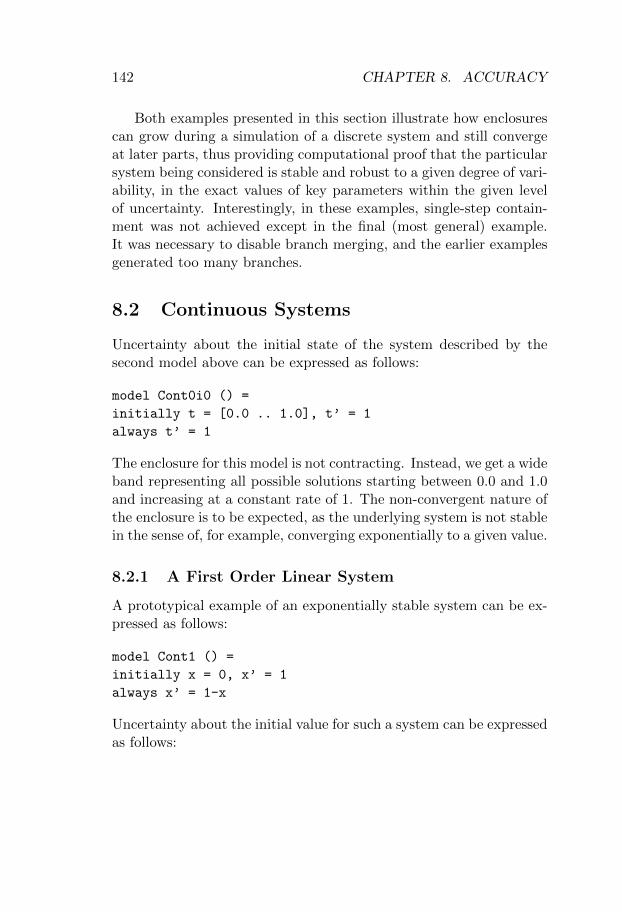
142 CHAPTER 8. ACCURACY
Both examples presented in this section illustrate how enclosurescan grow during a simulation of a discrete system and still convergeat later parts, thus providing computational proof that the particularsystem being considered is stable and robust to a given degree of vari-ability, in the exact values of key parameters within the given levelof uncertainty. Interestingly, in these examples, single-step contain-ment was not achieved except in the final (most general) example.It was necessary to disable branch merging, and the earlier examplesgenerated too many branches.
8.2 Continuous Systems
Uncertainty about the initial state of the system described by thesecond model above can be expressed as follows:
model Cont0i0 () =
initially t = [0.0 .. 1.0], t’ = 1
always t’ = 1
The enclosure for this model is not contracting. Instead, we get a wideband representing all possible solutions starting between 0.0 and 1.0and increasing at a constant rate of 1. The non-convergent nature ofthe enclosure is to be expected, as the underlying system is not stablein the sense of, for example, converging exponentially to a given value.
8.2.1 A First Order Linear System
A prototypical example of an exponentially stable system can be ex-pressed as follows:
model Cont1 () =
initially x = 0, x’ = 1
always x’ = 1-x
Uncertainty about the initial value for such a system can be expressedas follows:
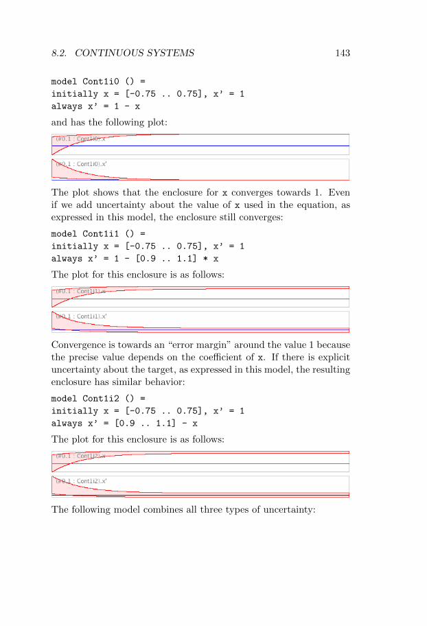
8.2. CONTINUOUS SYSTEMS 143
model Cont1i0 () =
initially x = [-0.75 .. 0.75], x’ = 1
always x’ = 1 - x
and has the following plot:
The plot shows that the enclosure for x converges towards 1. Evenif we add uncertainty about the value of x used in the equation, asexpressed in this model, the enclosure still converges:
model Cont1i1 () =
initially x = [-0.75 .. 0.75], x’ = 1
always x’ = 1 - [0.9 .. 1.1] * x
The plot for this enclosure is as follows:
Convergence is towards an “error margin” around the value 1 becausethe precise value depends on the coefficient of x. If there is explicituncertainty about the target, as expressed in this model, the resultingenclosure has similar behavior:
model Cont1i2 () =
initially x = [-0.75 .. 0.75], x’ = 1
always x’ = [0.9 .. 1.1] - x
The plot for this enclosure is as follows:
The following model combines all three types of uncertainty:
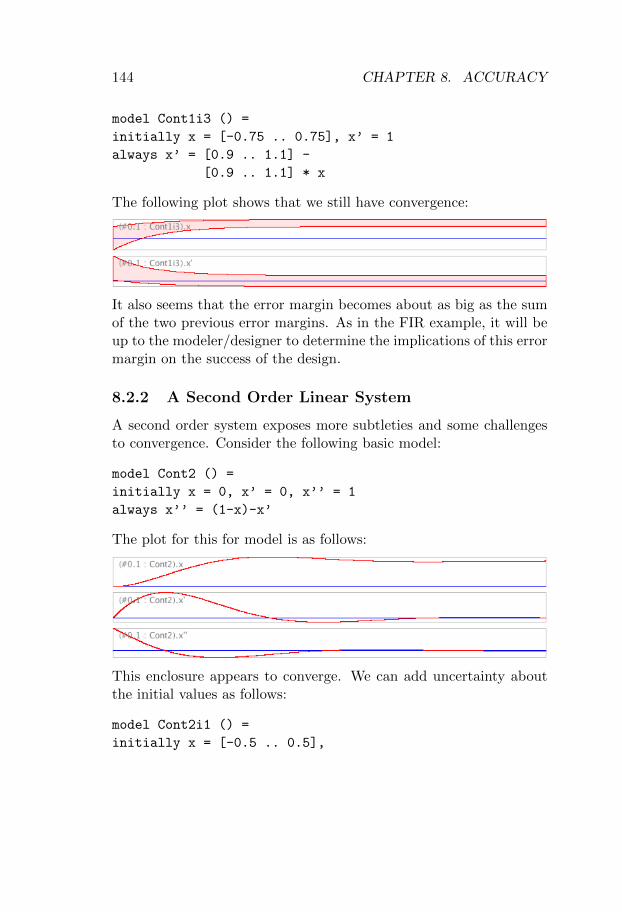
144 CHAPTER 8. ACCURACY
model Cont1i3 () =
initially x = [-0.75 .. 0.75], x’ = 1
always x’ = [0.9 .. 1.1] -
[0.9 .. 1.1] * x
The following plot shows that we still have convergence:
It also seems that the error margin becomes about as big as the sumof the two previous error margins. As in the FIR example, it will beup to the modeler/designer to determine the implications of this errormargin on the success of the design.
8.2.2 A Second Order Linear System
A second order system exposes more subtleties and some challengesto convergence. Consider the following basic model:
model Cont2 () =
initially x = 0, x’ = 0, x’’ = 1
always x’’ = (1-x)-x’
The plot for this for model is as follows:
This enclosure appears to converge. We can add uncertainty aboutthe initial values as follows:
model Cont2i1 () =
initially x = [-0.5 .. 0.5],
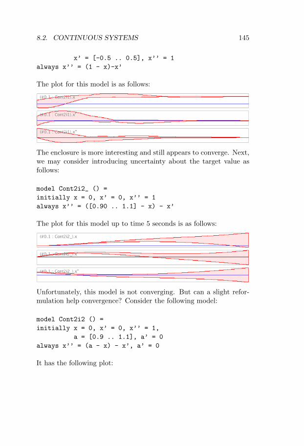
8.2. CONTINUOUS SYSTEMS 145
x’ = [-0.5 .. 0.5], x’’ = 1
always x’’ = (1 - x)-x’
The plot for this model is as follows:
The enclosure is more interesting and still appears to converge. Next,we may consider introducing uncertainty about the target value asfollows:
model Cont2i2_ () =
initially x = 0, x’ = 0, x’’ = 1
always x’’ = ([0.90 .. 1.1] - x) - x’
The plot for this model up to time 5 seconds is as follows:
Unfortunately, this model is not converging. But can a slight refor-mulation help convergence? Consider the following model:
model Cont2i2 () =
initially x = 0, x’ = 0, x’’ = 1,
a = [0.9 .. 1.1], a’ = 0
always x’’ = (a - x) - x’, a’ = 0
It has the following plot:
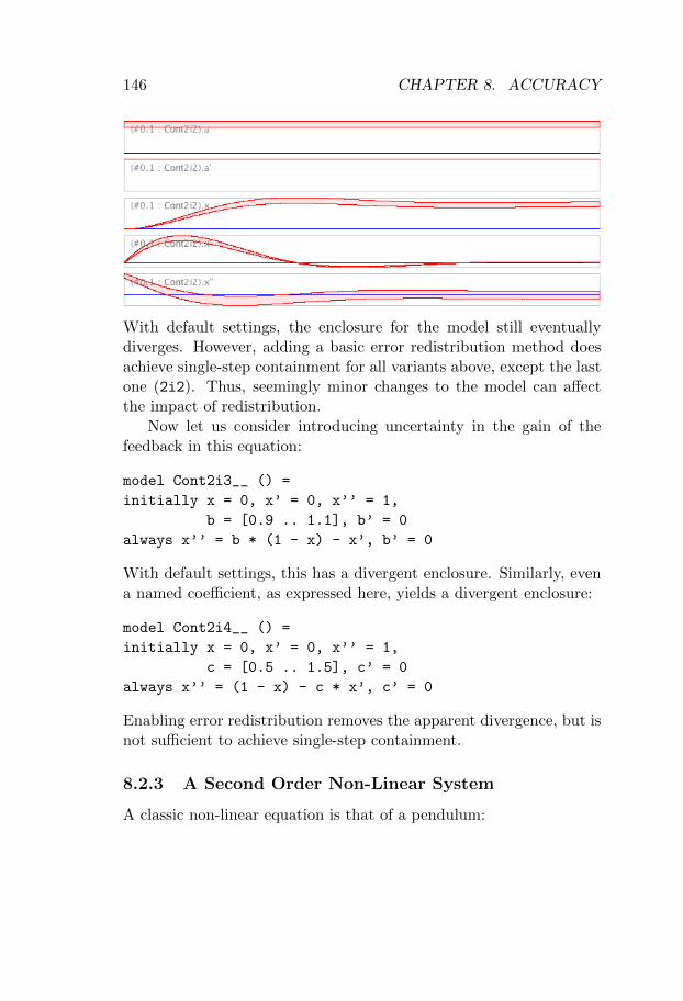
146 CHAPTER 8. ACCURACY
With default settings, the enclosure for the model still eventuallydiverges. However, adding a basic error redistribution method doesachieve single-step containment for all variants above, except the lastone (2i2). Thus, seemingly minor changes to the model can affectthe impact of redistribution.
Now let us consider introducing uncertainty in the gain of thefeedback in this equation:
model Cont2i3__ () =
initially x = 0, x’ = 0, x’’ = 1,
b = [0.9 .. 1.1], b’ = 0
always x’’ = b * (1 - x) - x’, b’ = 0
With default settings, this has a divergent enclosure. Similarly, evena named coefficient, as expressed here, yields a divergent enclosure:
model Cont2i4__ () =
initially x = 0, x’ = 0, x’’ = 1,
c = [0.5 .. 1.5], c’ = 0
always x’’ = (1 - x) - c * x’, c’ = 0
Enabling error redistribution removes the apparent divergence, but isnot sufficient to achieve single-step containment.
8.2.3 A Second Order Non-Linear System
A classic non-linear equation is that of a pendulum:
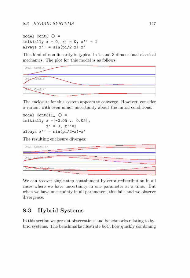
8.3. HYBRID SYSTEMS 147
model Cont3 () =
initially x = 0, x’ = 0, x’’ = 1
always x’’ = sin(pi/2-x)-x’
This kind of non-linearity is typical in 2- and 3-dimensional classicalmechanics. The plot for this model is as follows:
The enclosure for this system appears to converge. However, considera variant with even minor uncertainty about the initial conditions:
model Cont3i1_ () =
initially x =[-0.05 .. 0.05],
x’ = 0, x’’=1
always x’’ = sin(pi/2-x)-x’
The resulting enclosure diverges:
We can recover single-step containment by error redistribution in allcases where we have uncertainty in one parameter at a time. Butwhen we have uncertainty in all parameters, this fails and we observedivergence.
8.3 Hybrid Systems
In this section we present observations and benchmarks relating to hy-brid systems. The benchmarks illustrate both how quickly combining
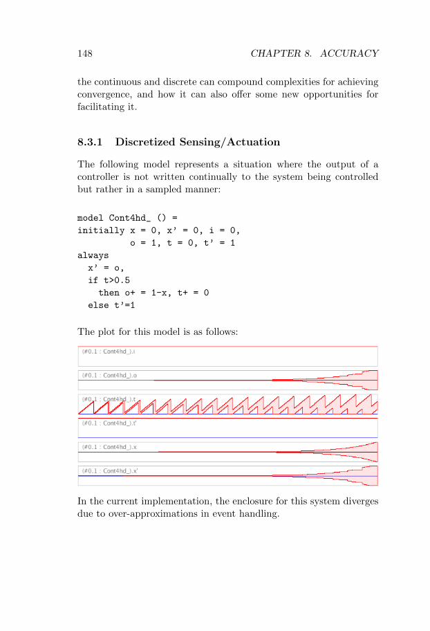
148 CHAPTER 8. ACCURACY
the continuous and discrete can compound complexities for achievingconvergence, and how it can also offer some new opportunities forfacilitating it.
8.3.1 Discretized Sensing/Actuation
The following model represents a situation where the output of acontroller is not written continually to the system being controlledbut rather in a sampled manner:
model Cont4hd_ () =
initially x = 0, x’ = 0, i = 0,
o = 1, t = 0, t’ = 1
always
x’ = o,
if t>0.5
then o+ = 1-x, t+ = 0
else t’=1
The plot for this model is as follows:
In the current implementation, the enclosure for this system divergesdue to over-approximations in event handling.
8.3. HYBRID SYSTEMS 149
8.3.2 Zeno Systems
A final and important type of system that is useful for evaluating theextent to which an implementation realizes the proposed principle isZeno systems [KTB+]. Such systems exhibit an infinite number ofdiscrete changes over a finite time interval. Zeno behavior is knownto be a phenomenon unique to hybrid systems, naturally arising inmodels of mechanical systems, control systems, and others.
A classic example of a model that exhibits Zeno behavior is abouncing ball:
model Hybrid1 () =
initially
x = 10, x’ = 0, x’’ = -10
always
claim x>=0,
if x == 0 && x’ < 0
then x’+ = -x’/2
else x’’ = -10
The variable x represents the height of a ball that falls to the ground.Upon impact with the ground, the ball bounces (switches direction)with half the speed. The claim statement is essentially syntacticsugar for a conditional that leads to blocking the system (having nosolution) in the else branch. Analysis of the model would reveal thatthe bouncing speed becomes zero after a finite amount of time, knownas the Zeno time. However, the ball would have to bounce a countablyinfinite number of times before reaching this point.
Previous work [KTB+] shows that it is possible to simulate suchmodels past the Zeno point, using a fixed-point computation on enclo-sures during simulation. However, such enclosures are not necessarilyconverging past the Zeno point. They generally have the followingshape:
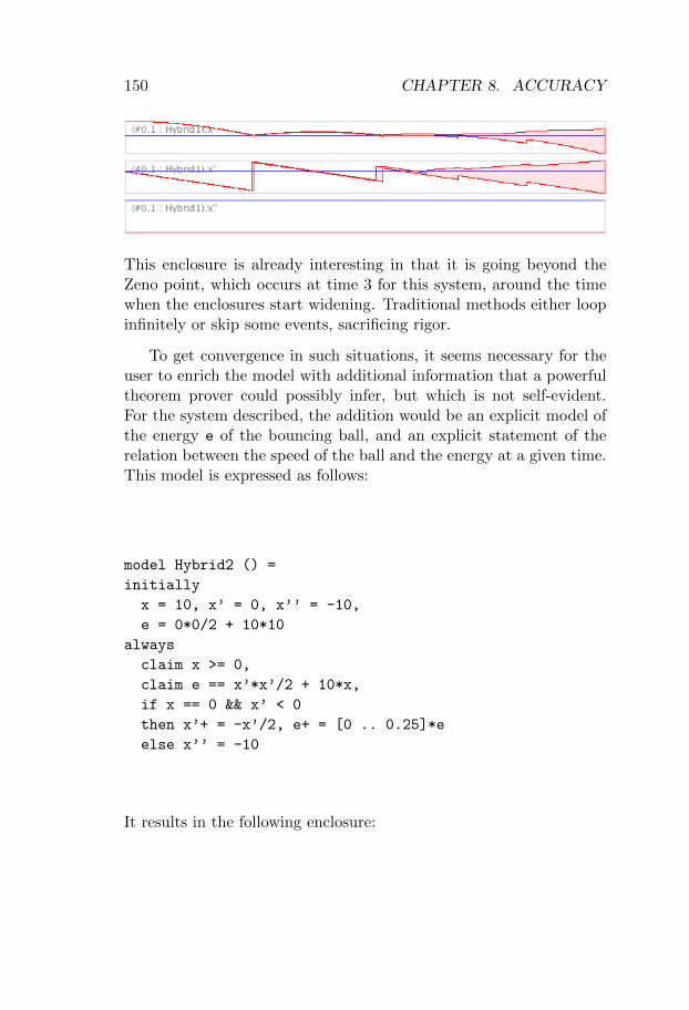
150 CHAPTER 8. ACCURACY
This enclosure is already interesting in that it is going beyond theZeno point, which occurs at time 3 for this system, around the timewhen the enclosures start widening. Traditional methods either loopinfinitely or skip some events, sacrificing rigor.
To get convergence in such situations, it seems necessary for theuser to enrich the model with additional information that a powerfultheorem prover could possibly infer, but which is not self-evident.For the system described, the addition would be an explicit model ofthe energy e of the bouncing ball, and an explicit statement of therelation between the speed of the ball and the energy at a given time.This model is expressed as follows:
model Hybrid2 () =
initially
x = 10, x’ = 0, x’’ = -10,
e = 0*0/2 + 10*10
always
claim x >= 0,
claim e == x’*x’/2 + 10*x,
if x == 0 && x’ < 0
then x’+ = -x’/2, e+ = [0 .. 0.25]*e
else x’’ = -10
It results in the following enclosure:
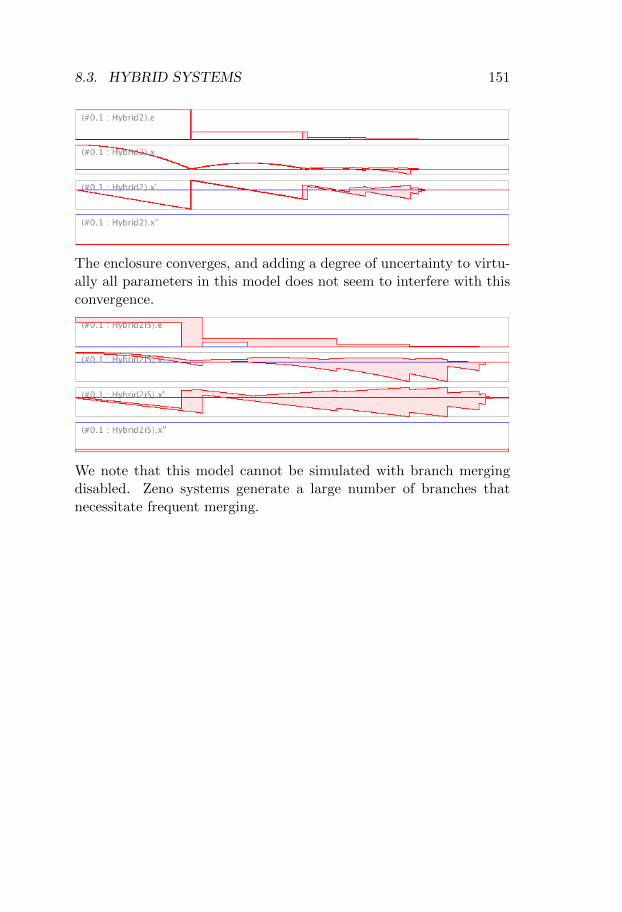
8.3. HYBRID SYSTEMS 151
The enclosure converges, and adding a degree of uncertainty to virtu-ally all parameters in this model does not seem to interfere with thisconvergence.
We note that this model cannot be simulated with branch mergingdisabled. Zeno systems generate a large number of branches thatnecessitate frequent merging.
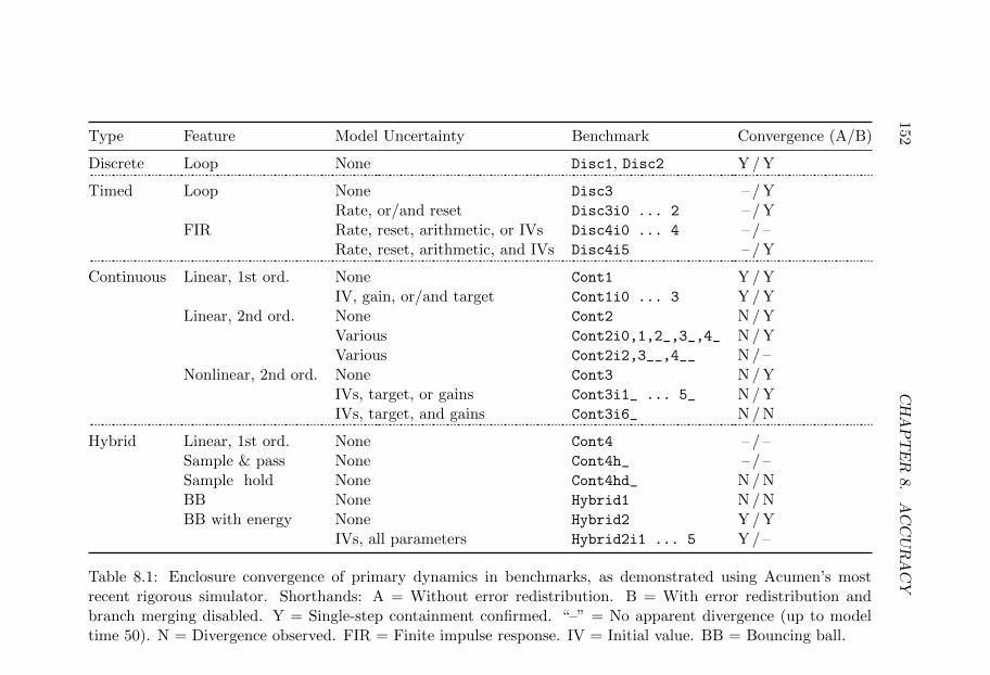
152
CHAPTER
8.ACCURACY
Type Feature Model Uncertainty Benchmark Convergence (A/B)
Discrete Loop None Disc1, Disc2 Y / Y
Timed Loop None Disc3 – / YRate, or/and reset Disc3i0 ... 2 – / Y
FIR Rate, reset, arithmetic, or IVs Disc4i0 ... 4 – / –Rate, reset, arithmetic, and IVs Disc4i5 – / Y
Continuous Linear, 1st ord. None Cont1 Y / YIV, gain, or/and target Cont1i0 ... 3 Y / Y
Linear, 2nd ord. None Cont2 N / YVarious Cont2i0,1,2_,3_,4_ N / YVarious Cont2i2,3__,4__ N / –
Nonlinear, 2nd ord. None Cont3 N / YIVs, target, or gains Cont3i1_ ... 5_ N / YIVs, target, and gains Cont3i6_ N / N
Hybrid Linear, 1st ord. None Cont4 – / –Sample & pass None Cont4h_ – / –Sample hold None Cont4hd_ N / NBB None Hybrid1 N / NBB with energy None Hybrid2 Y / Y
IVs, all parameters Hybrid2i1 ... 5 Y / –
Table 8.1: Enclosure convergence of primary dynamics in benchmarks, as demonstrated using Acumen’s mostrecent rigorous simulator. Shorthands: A = Without error redistribution. B = With error redistribution andbranch merging disabled. Y = Single-step containment confirmed. “–” = No apparent divergence (up to modeltime 50). N = Divergence observed. FIR = Finite impulse response. IV = Initial value. BB = Bouncing ball.
Chapter 9
Conclusion
This thesis described rigorous simulation, an approach to analyzinghybrid systems that combines the ease of use of simulation with therigor of verification. It presented a formal specification of a rigoroussimulator integrated into the modeling and simulation tool Acumen.A case study and a collection of benchmarks were used to evaluatethe approach.
9.1 Summary of Contributions
The main contributions of this thesis are as follows:
1. The syntax, denotational semantics and operational semanticsof a subset of the Acumen language are formally specified (Chap-ters 4 and 5). The specification leaves out the details of thevalidated numerical primitives that the operational semanticsis built on, and instead specifies these in terms of the propertiesrequired to prove soundness. The purpose is to separate con-cerns, making the semantics as general as possible. Preliminaryresults toward a proof of soundness of the operational seman-tics with respect to the denotational semantics are presented(Appendix A).
2. A a modeling environment that includes both traditional and
153
154 CHAPTER 9. CONCLUSION
rigorous simulators for the Acumen language is described (Chap-ter 6). The implementation and its source code are freely avail-able under a permissive license.
3. A case study and a collection of benchmarks that illustrate thefeasibility of the rigorous simulator are presented (Chapters 7and 8).
9.2 Lessons Learned
The main lesson learned during this work is that simulation can beboth practical and rigorous, but that achieving these goals requiresan effort that spans multiple disciplines. Practicality is a subtle mat-ter. It is subjective, and depends both on the user and on the kind ofproblem that the user wants to simulate. Being practical touches onissues as varied as supporting a flexible syntax, supporting numericalmethods that produce informative results, providing several flexibleviews of the simulation output, providing actionable error messages,and making the simulator’s user interface convenient. The notion ofrigor is more objective. However, achieving it in a tool requires knowl-edge of many domains, including mathematics, computer science andsoftware engineering. From mathematics, rigorous simulation relieson numerical methods and real analysis. From computer science, for-mal semantics is useful to precisely specify the modeling formalismand its properties. Software engineering practices such as testing areneeded to realize the theory in an implementation. Combining all ofthese domains becomes a challenge on the level of terminology andnotation. Finding a language that is familiar without carrying thewrong connotations thus becomes a challenge.
The rest of this section describes some specific lessons learnedduring this work. Some of them relate to language design and spec-ification. Others relate to the difficulty of maintaining soundness inan implementation of a rigorous simulator, in particular when it isintegrated with a traditional simulator.
9.2. LESSONS LEARNED 155
9.2.1 The Role of Properties in Semantics
A specification of a semantics can benefit from leaving out details. Forexample, in this thesis, the operational semantics (Section 5.8) is givenin terms of numerical primitives whose precise definitions are leftout. Instead, the primitives are specified as properties (Section 5.7.2).These properties are chosen to be only as specific as is necessary toprove the soundness of the operational semantics with respect to thedenotational semantics. This approach has several benefits. Leavingout details keeps the operational semantics minimal, by separatingtreatment of the simulation algorithm from the that of the primitivesit depends on. Doing so also makes the operational semantics general,in that any definition of a primitive that satisfies the correspondingproperties is compatible with the operational semantics.
9.2.2 Equations Versus Assignments
Early versions of the implementation interpreted equations as assign-ments, that is, statements that mutate the state as soon as they areprocessed by the interpreter. Such an interpretation is incompati-ble with how differential equations are solved in mathematics, whichrequires that sequences of equations (Section 3.3) are processed inparallel. Two different approaches were taken to implement this se-mantics. In the optimized traditional interpreter, two copies of thestate are maintained: one that is updated during interpretation andanother that is used to look up values of variables. In the referencetraditional interpreter and enclosure interpreter, the same issue issolved by flattening the AST into a system of equations, and passingthis system to a solver.
9.2.3 Translations as a Design Tool
Translations can be a useful tool when developing a language, as theycan help to uncover problems. In Section 4.2 we saw an exampleof this which shows that some translations can affect the rigoroussimulation result of a model. A rigorous simulator must evaluate
156 CHAPTER 9. CONCLUSION
Boolean expressions in a way that takes uncertainties in state vari-ables into account. Just like interval arithmetic causes identities suchas x−x = 0 to break, a set extension of Boolean logic causes identitiessuch as p ∧ ¬p ⇐⇒ false to break1. To avoid a loss of precision, atranslation must therefore not produce such terms, or they must beidentified and eliminated during evaluation. We discovered this issuewhen validating the translations described in Section 4.2 using ourimplementation.
9.2.4 Soundness Pitfalls
Developing a rigorous simulator requires maintaining a correctnessguarantee, fundamentally provided by interval arithmetic, throughouta code base that may span many thousands of lines.
9.2.4.1 Parsing
Before the simulation can start, the tool needs to parse the textualmodel into a data structure, typically an abstract syntax tree, thatcan then be compiled or interpreted. Parsing libraries typically comewith parsers for numerical literals. Seeing as these typically parseliterals into floating-point numbers, any non-representable number(such as 0.1), will be rounded. Even if the resulting floating-pointnumber is then converted into an interval before simulation, thisparsing is unsound. Because 0.1 will be converted to a thin inter-val (whose end-points are equal), a check such as 10 ∗ 0.1 > 1 mayreturn true, depending on the rounding mode used during parsing.To solve this problem, parsing of numeric constants can be deferreduntil they are interpreted (e.g. as intervals), or by parsing into anarbitrary-precision numeric type, such as rational numbers.
1 When p is the set {true, false} then p ∧ ¬p = {p1 ∧ ¬p2 | p1 ∈ p, p2 ∈ p} ={true, false}, even though the formula is equivalent to false for any point value ofp. This effect is analogous to dependency [Moo] in interval arithmetic.
9.3. FUTURE WORK 157
9.2.4.2 Constants
Numerical constants such a π are useful for modeling, especially incombination with trigonometric functions. The correct way to addthese to a rigorous simulator is to provide a high-precision intervalthat encloses the true value. It is, for example, not sufficient to con-vert the constant as obtained from an arbitrary-precision numericallibrary. This value must be truncated by one significand, using thelast bit of precision to obtain the bounds for the enclosing interval.
9.2.4.3 Preprocessing
Most simulation tools perform some kind of preprocessing before sim-ulation, be it converting the model into an executable form (e.g. in-dex reduction of DAEs), or for performance (e.g. partial evaluation).When transformations involve numerical operations, such as thoseperformed during constant folding, they must be performed with asound arithmetic. For example, this could be exact arithmetic of anarbitrary-precision numeric type, or interval arithmetic.
9.2.4.4 Safe Comparisons
During rigorous simulation, different kinds of approximations mustbe compared. Often, operations can be safely performed on over-approximations of the operands, but this is sometimes unsound. Forexample, to detect a fixed point in a reachability computation, it isnecessary to check if one state is covered by another state. Such asubset containment check must either be performed directly on theoperand types, or with an over-approximation of the possible subsetand an under-approximation of the possible superset.
9.3 Future Work
This section outlines work needed to further support the thesis of thisdissertation (Section 1.2). The foundations for rigorous simulation
158 CHAPTER 9. CONCLUSION
are there, and development in several different directions is possibleto increase the practicality of the approach.
9.3.1 A Richer Syntax and Semantics
To better support practical systems modeling, the rigorous simulatorneeds to be extended to the full Acumen language. This includesadding support for: vectors and matrices, including notation for up-dating parts of a matrix; dynamic creation, termination and move-ment of objects [BT]; and acausal modeling with DAEs [ZRT+].
The current implementation makes two kinds of fixpoint checksduring simulation. The first is used to check if a fixpoint is reached inthe intermediate enclosures computed within a single step. The otherchecks if the enclosure computed for the current step is included in theone for the previous step. To be able to detect fixpoints of periodicsystems, it is necessary to extend the horizon over which the fixpointis detected. The check could also be made more general by checkingfor coverings, rather than for containment in an individual state.
Acumen’s current semantics treats over-specified models, such as{x′ = f(x), x′ = g(x)}, as modeling errors. There are several con-ceivable alternatives that are natural in the setting of a rigoroussimulator. For example, {x′ = f(x), x′ = g(x)} could be inter-preted as the differential inclusion x′ ∈ [min(f, g) ..max(f, g)], where[min(f, g) ..max(f, g)] can be approximated by taking the enclosurehull of the solutions computed for x′ = f(x) and x′ = g(x) individu-ally.
In the immediate future, we would like to focus on better under-standing, and on improving the performance of, the current imple-mentation of rigorous simulation in Acumen. We plan to continue touse this implementation to explore better ways to reduce and controlbranching.
More precise simulations of models with uncertain initial statecan be achieved by splitting the uncertainties and running a separatesimulation for each combination of parts. We plan to add supportfor automating this kind of batch simulation into Acumen. Moreelaborate schemes are also possible, where the state is split during the
9.3. FUTURE WORK 159
course of the simulation. Such schemes are powerful but more difficultto implement efficiently, because the number of cases to consider whensplitting a state increases exponentially in the number of subdivisions.This process can be prohibitively expensive if it is done iteratively, asin the case of a simulation algorithm.
From discussions with industrial practitioners, it is also clear thatthere is user demand for stochastic modeling, such as assigning prob-ability distributions to variables. A simple approach to simulatingsuch models is by splitting the probability distributions and runningeach part as a separate simulation.
9.3.2 Visualization
Being able to execute the same model using both the rigorous andtraditional simulators has been useful in great part because the lattersupports 3D visualization of the simulation results. Preliminary workon extending this functionality to the rigorous simulator was devel-oped in the thesis of Pawlik and Andersson [PA], where the simulationresult is visualized by sampling and rough (box) over-approximation.This work can be taken further by tightening the over-approximation.

160 CHAPTER 9. CONCLUSION

Appendices
161

Appendix A
Preliminary Results
In this appendix I establish that the operational semantics encloses afinitary denotational semantics that is also defined in this appendix.Establishing this result requires several new definitions and lemmas.Among these are two monotonicity results (Propositions A.0.3 andA.0.2), as well as transition relations and functions (Definitions 5.7.2,A.0.6 and A.0.8) that reflect the imprecision that results from thediscretization of time in the operational semantics. The results pre-sented in this appendix use induction, following the structure of thedefinition of the finitary denotational semantics. I believe that theywill be useful in proving Conjecture 5.9.2, though that proof will likelybe based on the Tarski fixpoint theorem [Tar].
Definition A.0.1 (Finitary Evolution of a Hybrid System). The fini-tary evolution of a hybrid system (F, J) ∈ H is a function [[[(F, J)]]] :P(S) → P(T × S) from the set of states to the set of time-states.Given an initial closed set of states S, the finitary evolution [[[(F, J)]]]Sof (F, J) from S is defined as follows:
[[[(F, J)]]]S
s ∈ S(0, s) ∈ [[[(F, J)]]]S
(t, s1) ∈ [[[(F, J)]]]S (F, J), s1δ- s2
(t+ δ, s2) ∈ [[[(F, J)]]]S
163
164 APPENDIX A. PRELIMINARY RESULTS
�
Proposition A.0.2. Whenever q ∈ m ∈Mµ and d1, d2 ∈ D then
d2 ⊆ d2 ∧ q 6∈ active(m, d1) =⇒ q 6∈ active(m, d2)
Proof.
q 6∈ active(m, d1)=⇒ ∀if e thenA ∈ m. true 6∈ {[[e]]s | s ∈ d1} (by Def 5.7.6 2c)=⇒ ∀if e thenA ∈ m. true 6∈ {[[e]]s | s ∈ d2} (as d2 ⊆ d1)=⇒ q 6∈ active(m, d2)
Proposition A.0.3. The operational semantics m ` q1, (t, d) h↪−−→ Zis inclusion isotonic with respect to its enclosure parameter d.
∀q ∈ m ∈Mµ, t ∈ T, d1, d2 ∈ D, h ∈ T.d2 ⊆ d1 ∧ (m ` q, (t, d1) h↪−−→ Z1) =⇒
(m ` q, (t, d2) h↪−−→ Z2) ∧ [[Z2]] ⊆ [[Z1]]
Proof. By structural induction on the derivation of ↪−→.
Base case : The non-recursive cases are that of the Blocked rule andthe Continuous rule when m = {q}.
Case Blocked : We know that q 6∈ active(m, d1) and Z1 = ∅. Thenq 6∈ active(m, d2) by Proposition A.0.2, and thus m ` q, (t, d2) h↪−→ Z2
by the Blocked rule and [[Z2]] = ∅ ⊆ [[Z1]].
Case Continuous, m = {q} : We know that Z1 = {d1(0 .. h)/d12@(0 .. h]}
and q ∈ active(m, d1). Then q ∈ active(m, d2) by Proposition A.0.2and m ` q, (t, d2)
h↪−→ Z2 by the Continuous rule. Further, Z2 ={d2(0 .. h)/d
22@(0 .. h]} because m1 = ∅. Now
d2 ⊆ d1=⇒ (d2(0 .. h) ⊆ d
1(0 .. h) ∧ d
22 ⊆ d12) (by Def 5.7.6 4a)
=⇒ [[Z2]] ⊆ [[Z1]] (by Def 5.6.4)
165
which completes the base case.
Inductive case : The recursive rules are Discrete and Continuous whenm 6= {q}.
Case Discrete : We know that
m ` q, (t, d1) h↪−→ Z1
d12 = reset(q, d1)
{m ` q′, (t, d12)h↪−→ Z1
q′}q′∈m
Z1 = {d12@t} ∪⋃q′∈m Z
1q′
If q1 6∈ active(m, d2) then Z2 = ∅ ⊆ Z1. Otherwise we have d22 =reset(q1, d2) with d22 ⊆ d12 by Definition 5.7.6 3a and
{m ` q′, (t, d22)h↪−→ Z2
q′}q′∈m
with ∀q ∈ m. Z2q′ ⊆ Z1
q′ by the induction hypothesis. Therefore
m ` q, (t, d2) h↪−→ Z2, with Z2 = {d22@t} ∪⋃q′∈m Z
2q′
Finally [[d22@t]] ⊆ [[d12@t]] by Definition 5.6.4 and thus also [[Z2]] ⊆[[Z1]], which completes the case for Discrete.
Case Continuous, m 6= {q} ∧ t = [0] ∧ d13 = d12 : We know that
m ` q, (t, d1) h↪−→ Z1
(d1(0 .. h), d12) = solveIVP(q, d1, h)
{m ` q′, ((0 .. h), d1(0 .. h))h↪−→ Z1
q′}q′∈m1
Z1 = {d1(0 .. h)/d12@(0 .. h]} ∪
⋃q′∈m1
Z1q′
Now, if q1 6∈ active(m, d1) then [[Z2]] = ∅ ⊆ [[Z1]]. Otherwise we notethat (d2(0 .. h), d
22) = solveIVP(q, d2, h) with d2(0 .. h) ⊆ d1(0 .. h) ∧ d
22 ⊆ d12
by Definition 5.7.6 4a. Therefore
{m ` q′, ((0 .. h), d2(0 .. h))h↪−→ Z2
q′}q′∈m1 , with ∀q′ ∈ m1. [[Z2
q′ ]] ⊆ [[Z1q′ ]]
166 APPENDIX A. PRELIMINARY RESULTS
by the induction hypothesis. Finally,
[[d2(0 .. h)/d22@(0 .. h]]] ⊆ [[d1(0 .. h)/d
12@(0 .. h]]]
by Definition 5.6.4 and thus also [[Z2]] ⊆ [[Z1]], which completes thecase for Continuous.
Lemma A.0.4.
∀q ∈ Q. H(q), s1δ- s2 =⇒ q, s1
δ- s2
Proof. Let q ∈ Q and assume that H(q), s1δ- s2. There are two
cases to check: when δ = 0 and when δ > 0.
Case δ = 0 : The statement follows directly from Definition 5.4.5.
Case δ > 0 : Since guard(uncondition(q)) = true, Proposition 5.3.10gives us that π1H(uncondition(q)) ⊆ π1H(q).
Thus H(uncondition(q)), s1δ - s2, which in turn gives us that
q, s1δ- s2 by Definition 5.4.5.
Lemma A.0.5.
∀m ∈Mµ.H(m), s1δ- s2 =⇒ m, s1
δ- s2
Proof. Assume that H(m), s1δ- s2. There are two cases for δ that
we must check.
Case δ = 0: Then ∃q ∈ m. H(q), s1δ- s2 by Definitions 5.4.5 and
5.7.2. Then the statement follows directly from Definition 5.7.2.
Case δ > 0: Then by Definition 5.4.5 there exists a function x definedover [0 .. δ] such that x(0) = s1, x(δ) = s2 and
∀t ∈ [0 .. δ]. (x(t), x′(t)) ∈ π1(H(m))
Because m is in partitioned form (Definition 4.2.6), the guards ofthe modes in m partition x into (disjoint, consecutive) segments
167
with domains xσ(t) with time domains Tσ such that ∃qσ ∈ m. ∀t ∈T. (xσ(t), x′σ(t)) ∈ π1(H(qσ)). Then qσ, xσ(T ) - x′σ(T ) by Propo-sition 5.3.10 and Lemma A.0.4. Thus, by Definition 5.7.2, we get
m,xσ(T ) - x′σ(T ) for each segment and, consequently, we also get
m,x(0) - x(δ).
Definition A.0.6 (Evolution of a Mode). The evolution of a modeq ∈ m is a function [[[m ` q]]] : Pclosed(T × S) → Pclosed(T × S) fromthe set of closed time-states to itself. Given an initial closed set oftime-states I ∈ Pclosed(T × S), the evolution [[[m ` q]]]I of q from I isdefined as follows:
[[[m ` q]]]I
(t, s1) ∈ I q, s1δ- s2
(t+ δ, s2) ∈ [[[m ` q]]]I(t, s1) ∈ [[[m ` q]]]I m, s1
δ- s2
(t+ δ, s2) ∈ [[[m ` q]]]I
�
Proposition A.0.7.iso([[[m ` q]]]·)
Proof. By structural induction on the derivation of [[[m ` q]]]·. As-sume that
I2 ⊆ I1 ⊆ T× D (A.1)
[[[m ` q]]]I1 ↓ (A.2)
There are two rules in Definition A.0.6 by which (t + δ, s2) ∈ [[[m `q]]]I2: one that is not recursive (the base case) and one that is recur-sive (the inductive case).
Base case (t, s2) ∈ I1 ∧ q, s1δ- s2 : Then (t, s1) ∈ I1 by (A.1) and
thus (t+ δ, s2) ∈ [[[m ` q]]]I1 by Definition A.0.6.
Inductive case (t, s1) ∈ [[[m ` q]]]I2 ∧ m, s1δ- s2 : Then (t, s1) ∈
[[[m ` q]]]I1 by the induction hypothesis and (m, s1δ- s2) by (A.2).
168 APPENDIX A. PRELIMINARY RESULTS
Thus (t+ δ, s2) ∈ [[[m ` q]]]I2 by Definition A.0.6.
Definition A.0.8 (Evolution of a Model). The evolution of a modelm is a function [[[m]]] : Pclosed(S)→ Pclosed(T×S) from the set of closedtime-states to itself. Given an initial set of states S, the evolution[[[m]]]S of m from S is defined as follows:
[[[m]]]Ss ∈ S
(0, s) ∈ [[[m]]]S
(t, s1) ∈ [[[m]]]S m, s1δ- s2
(t+ δ, s2) ∈ [[[m]]]S
�
Lemma A.0.9. Let m ∈Mµ, S ∈ Pclosed(S) and I = {0} × S then
[[[H(m)]]]S ⊆ [[[m]]]S
Proof. By induction on the structure of the derivation of [[[H(m)]]]Sthat follows the rules for [[·]]· in Definition A.0.1. There are three casesby which (t, s) ∈ [[[H(m)]]]S. Two of these cases correspond to rulesin Definition A.0.1. The third corresponds to [[[H(m)]]]S being closed,meaning that (t, s) is on the boundary of [[[H(m)]]]S. In each case weneed to show that (t, s) ∈ [[[m]]]S.
Case (t, s) ∈ I : Then (t, s) ∈ [[[m]]]S directly by Definition A.0.8.
Case (t, s) /∈ I : We know that
(t1, s1) ∈ [[[(F, J)]]]S [[[H(m)]]]S, s1δ- s2 (t, s) = (t1 + δ, s2)
But then (t1, s1) ∈ [[[m]]]S by the induction hypothesis andm, s1δ- s2
by Lemma A.0.5. Thus (t1 + δ, s2) = (t, s) ∈ [[[m]]]S by Defini-tion A.0.8.
Case (t, s) is in the boundary of [[[H(m)]]]S : By the first two caseswe have shown that all (t, s) in the interior of [[[H(m)]]]S are also in
169
[[[m]]]S. Since by definition [[[m]]]S is a closed set, it must also containthe boundary of [[[H(m)]]]S.
Lemma A.0.10. Let m ∈Mµ, S ∈ Pclosed(S) and I = {0}×S. Then
[[[m]]]S ⊆ I ∪⋃q∈m
[[[m ` q]]]I
Proof. By structural induction on the derivation of [[[m]]]S.
Case s ∈ S : Then (t, s) = (0, s) ∈ I so the statement holds trivially.
Case (t1, s1) ∈ [[[m]]]S ∧ m, s1δ- s2 ∧ (t, s) = (t1 + δ, s2) :
Then ∃q1 ∈ m.q1, s1 δ- s2 by Definition 5.7.2. By the inductionhypothesis we can assume that
(t1, s1) ∈ I ∪⋃q∈m
[[[m ` q]]]I
so we need to consider two additional sub-cases.
Case (t1, s1) ∈ I : Then (t1 + δ, s2) ∈ [[[m ` q1]]]I.
Case (t1, s1) ∈⋃q∈m[[[m ` q]]]I : Then (t1, s1) ∈ [[[m ` q2]]]I for some
q2 ∈ m. But then (t1 + δ, s2) ∈ [[[m ` q2]]]I by Definition A.0.6 andDefinition 5.7.2.
Definition A.0.11 (Move). The function move : Q × (T × D) →Pclosed(T× D) is defined as follows:
move(q, I)
move(q, I) = closure({(t+ δ, s2) | (t, s1) ∈ I ∧ (q, s1δ- s2)})
�
170 APPENDIX A. PRELIMINARY RESULTS
Proposition A.0.12. When q ≡ if e then 〈x′i = ei〉i∈N and I ⊆ T× Sthen
move(q,move(q, I)) ⊆ move(q, I)
Proof. Let I1 = move(q, I), I2 = move(q, I1) and (t, s) ∈ I2. Then
there exists (t1, s1) ∈ I such that q, s1 - s2 ∧ q, s2 - s. But then
by Definition 5.7.2 we also have q, s1 - s and thus (t, s) ∈ I1.
Lemma A.0.13. Let q1 ∈ m, S ⊂ S, T ⊂ IR and I = T × S. Then
[[[m ` q1]]]I ⊆ I1 ∪⋃q∈m
[[[m ` q]]]I1 (A.3)
where I1 = move(q1, I).
Proof. By structural induction on the derivation of [[[m ` q1]]]I. LetS = I1 ∪
⋃q∈m[[[m ` q]]]I1.
Base case (t, s1) ∈ I and q1, s1δ- s2 : Then (t+δ, s2) ∈ move(q1, I) ⊆
S by Definition A.0.11.
Inductive case (t, s1) ∈ [[[m ` q1]]]I and m, s1δ- s2 : Then ∃q2 ∈
m. q2, s1δ- s2 by Definition 5.7.2. We have that (t, s1) ∈ S by the
induction hypothesis, and we need to show that (t+δ, s2) ∈ S. Thereare two cases to check: when (t, s1) ∈ I1 and when (t, s1) 6∈ I1.
Case (t, s1) ∈ I1 : Then (t+ δ, s2) ∈ move(q2, I1) ⊆ [[[m ` q2]]]I1 ⊆ S.
Case (t, s1) 6∈ I1 : Then ∃q3 ∈ m. (t, s1) ∈ [[[m ` q3]]]I1, and so(t+ δ, s2) ∈ [[[m ` q3]]]I1 ⊆ S by Definition A.0.6.
Corollary A.0.14. When q1 ≡ if e then 〈x′i = ei〉i∈N then
[[[m ` q1]]]I ⊆ I1 ∪⋃
q∈m\{q1}
[[[m ` q]]]I1
where I1 = move(q1, I).
171
Proof. Let S = I1 ∪⋃q∈m\{q1}[[[m ` q]]]I1. Lemma A.0.13 states that
[[[m ` q1]]]I ⊆ move(q1, I) ∪⋃q∈m
[[[m ` q]]] move(q1, I)
Thus it suffices to prove that
move(q1, I) ∪⋃q∈m[[[m ` q]]] move(q1, I)
⊆ move(q1, I) ∪⋃q∈m\{q1}[[[m ` q]]] move(q1, I)
or, equivalently
[[[m ` q1]]] move(q1, I) ⊆ move(q1, I)∪⋃
q∈m\{q1}
[[[m ` q]]] move(q1, I) (A.4)
We prove (A.4) by structural induction on the derivation of [[[m `q1]]] move(q1, I). There are two ways in which (t + δ, s2) ∈ [[[m `q1]]] move(q1, I) by Definition A.0.6.
Base case (t, s1) ∈ move(q1, I) ∧ q1, s1δ- s2 : Then (t + δ, s2) ∈
move(q1, I) ⊆ S by Definition A.0.11.
Inductive case (t, s1) ∈ [[[m ` q1]]] move(q1, I) ∧ m, s1δ- s2 : Then
∃q2 ∈ m. q2, s1δ- s2 by 5.7.2 and (t, s1) ∈ S by the induction
hypothesis.
Case (t, s1) ∈ move(q1, I) : Then (t+δ, s2) ∈ move(q2,move(q1, I)). Ifq2 = q1 then move(q2,move(q1, I)) = move(q1, I) by Proposition A.0.12,so (t + δ, s2) ∈ S. If q2 6= q1 then move(q2,move(q1, I)) ⊆ [[[m `q2]]] move(q1, I) by Lemma A.0.13, so again (t+ δ, s2) ∈ S.
Case (t, s1) 6∈ move(q1, I) : Then (t, s1) ∈ [[[m ` q3]]] move(q1, I) ⊆ Sfor some q3 ∈ m \ {q1}. But then we also have (t + δ, s2) ∈ [[[m `q3]]] move(q1, I) by Definition A.0.6, and thus (t+ δ, s2) ∈ S.
172 APPENDIX A. PRELIMINARY RESULTS
Lemma A.0.15 (Soundness With Respect to Finitary DenotationalSemantics When Starting From a Mode). Given a MicroAcumen modelm ∈ Mµ with state space S = RN, a mode q1 ∈ m, a time h > 0, andan enclosure d1, we have that
(m ` q1, (t, d1) h↪−−→ Zt) =⇒∀t ∈ T t. ([[[m ` q1]]]({t} × d1))|[0 .. h) ⊆ [[Zt]] (A.5)
where T [0] = {0}, T (0 .. h) = (0 .. h).
Proof. By structural induction on the derivation of ↪−→.
Base case : The only rule of Definition 5.8.2 that is not recursiveis Blocked. This rule works identically for I = {0} × d1 and I ={t} × d1 with t ∈ (0 .. h), so we prove the cases for t = [0] andt = (0 .. h) simultaneously. So, assume that m ` q1, (t, d1)
h↪−→ Zby the Blocked rule. Then [[Z]] = [[∅]] = ∅ active(m, d1) ↓ and q1 6∈active(m, d1). Thus, assumption 2c on the auxiliary function active,stated in Definition 5.7.6, gives us that
{s | s ∈ d1 ∧ [[guard(q1)]]s = true} = ∅
so by definitions 5.3.9 and 5.7.2
{s2 | s1 ∈ d1 ∧ (q1, s1 - s2)} = ∅
and thus ([[[m ` q1]]]I)|[0 .. h) = ∅ by Definition A.0.6.
Inductive case : The recursive rules are Discrete and Continuous.Lemma A.0.13 allows us to unfold the definition of [[[m ` q1]]] for anyI ⊆ T× S as follows:
([[[m ` q1]]]I)|[0 .. h) ⊆ (I1 ∪⋃q∈m
[[[m ` q]]]I1)|[0 .. h) (A.6)
whereI1 = {(t+ δ, s2) | (t, s1) ∈ I ∧ (q1, s1
δ- s2)} (A.7)
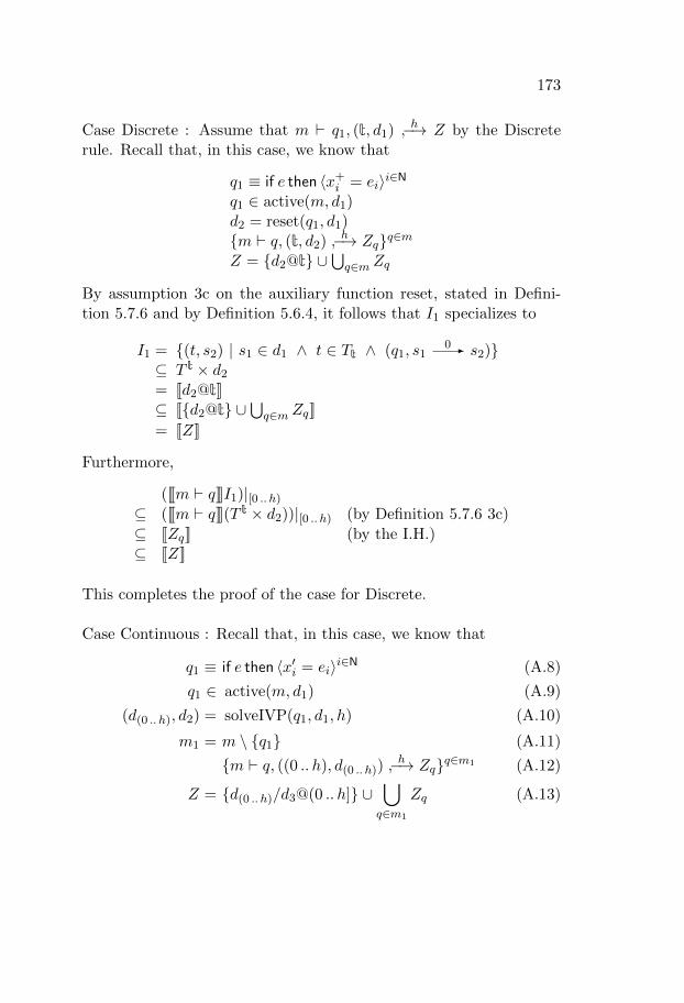
173
Case Discrete : Assume that m ` q1, (t, d1) h↪−→ Z by the Discreterule. Recall that, in this case, we know that
q1 ≡ if e then 〈x+i = ei〉i∈Nq1 ∈ active(m, d1)d2 = reset(q1, d1){m ` q, (t, d2) h↪−→ Zq}q∈mZ = {d2@t} ∪
⋃q∈m Zq
By assumption 3c on the auxiliary function reset, stated in Defini-tion 5.7.6 and by Definition 5.6.4, it follows that I1 specializes to
I1 = {(t, s2) | s1 ∈ d1 ∧ t ∈ Tt ∧ (q1, s10- s2)}
⊆ T t × d2= [[d2@t]]⊆ [[{d2@t} ∪
⋃q∈m Zq]]
= [[Z]]
Furthermore,
([[[m ` q]]]I1)|[0 .. h)⊆ ([[[m ` q]]](T t × d2))|[0 .. h) (by Definition 5.7.6 3c)
⊆ [[Zq]] (by the I.H.)⊆ [[Z]]
This completes the proof of the case for Discrete.
Case Continuous : Recall that, in this case, we know that
q1 ≡ if e then 〈x′i = ei〉i∈N (A.8)
q1 ∈ active(m, d1) (A.9)
(d(0 .. h), d2) = solveIVP(q1, d1, h) (A.10)
m1 = m \ {q1} (A.11)
{m ` q, ((0 .. h), d(0 .. h))h↪−→ Zq}q∈m1 (A.12)
Z = {d(0 .. h)/d3@(0 .. h]} ∪⋃q∈m1
Zq (A.13)
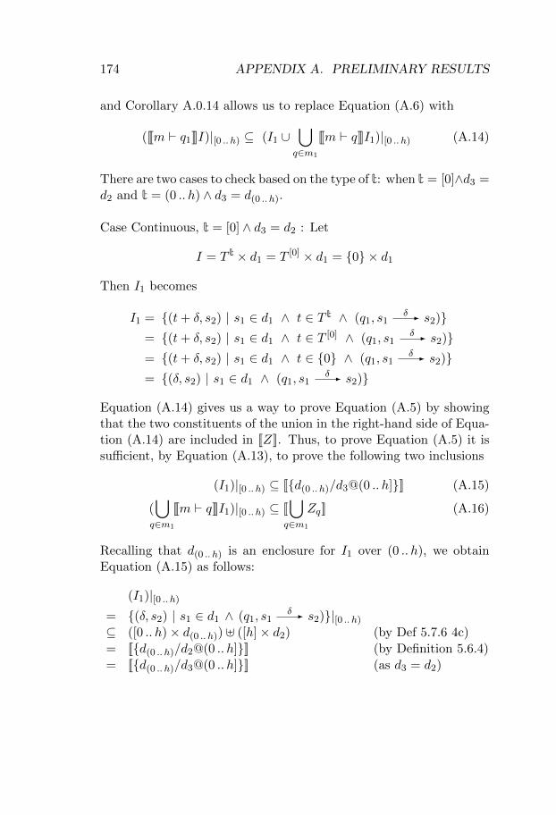
174 APPENDIX A. PRELIMINARY RESULTS
and Corollary A.0.14 allows us to replace Equation (A.6) with
([[[m ` q1]]]I)|[0 .. h) ⊆ (I1 ∪⋃q∈m1
[[[m ` q]]]I1)|[0 .. h) (A.14)
There are two cases to check based on the type of t: when t = [0]∧d3 =d2 and t = (0 .. h) ∧ d3 = d(0 .. h).
Case Continuous, t = [0] ∧ d3 = d2 : Let
I = T t × d1 = T [0] × d1 = {0} × d1
Then I1 becomes
I1 = {(t+ δ, s2) | s1 ∈ d1 ∧ t ∈ T t ∧ (q1, s1δ- s2)}
= {(t+ δ, s2) | s1 ∈ d1 ∧ t ∈ T [0] ∧ (q1, s1δ- s2)}
= {(t+ δ, s2) | s1 ∈ d1 ∧ t ∈ {0} ∧ (q1, s1δ- s2)}
= {(δ, s2) | s1 ∈ d1 ∧ (q1, s1δ- s2)}
Equation (A.14) gives us a way to prove Equation (A.5) by showingthat the two constituents of the union in the right-hand side of Equa-tion (A.14) are included in [[Z]]. Thus, to prove Equation (A.5) it issufficient, by Equation (A.13), to prove the following two inclusions
(I1)|[0 .. h) ⊆ [[{d(0 .. h)/d3@(0 .. h]}]] (A.15)
(⋃q∈m1
[[[m ` q]]]I1)|[0 .. h) ⊆ [[⋃q∈m1
Zq]] (A.16)
Recalling that d(0 .. h) is an enclosure for I1 over (0 .. h), we obtainEquation (A.15) as follows:
(I1)|[0 .. h)= {(δ, s2) | s1 ∈ d1 ∧ (q1, s1
δ- s2)}|[0 .. h)⊆ ([0 .. h)× d(0 .. h)) ] ([h]× d2) (by Def 5.7.6 4c)
= [[{d(0 .. h)/d2@(0 .. h]}]] (by Definition 5.6.4)
= [[{d(0 .. h)/d3@(0 .. h]}]] (as d3 = d2)
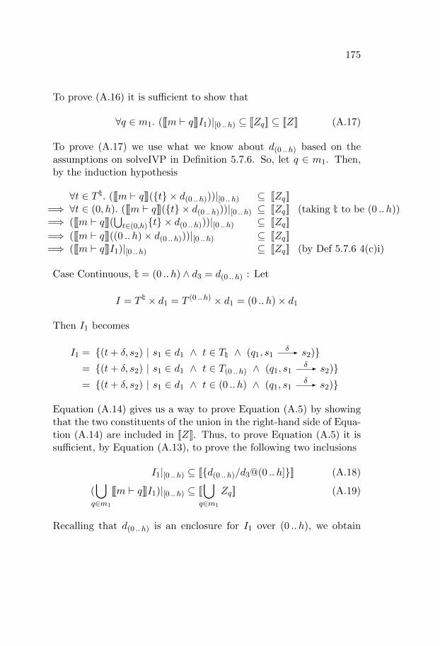
175
To prove (A.16) it is sufficient to show that
∀q ∈ m1. ([[[m ` q]]]I1)|[0 .. h) ⊆ [[Zq]] ⊆ [[Z]] (A.17)
To prove (A.17) we use what we know about d(0 .. h) based on theassumptions on solveIVP in Definition 5.7.6. So, let q ∈ m1. Then,by the induction hypothesis
∀t ∈ T t. ([[[m ` q]]]({t} × d(0 .. h)))|[0 .. h) ⊆ [[Zq]]
=⇒ ∀t ∈ (0, h). ([[[m ` q]]]({t} × d(0 .. h)))|[0 .. h) ⊆ [[Zq]] (taking t to be (0 .. h))
=⇒ ([[[m ` q]]](⋃t∈(0,h){t} × d(0 .. h)))|[0 .. h) ⊆ [[Zq]]
=⇒ ([[[m ` q]]]((0 .. h)× d(0 .. h)))|[0 .. h) ⊆ [[Zq]]
=⇒ ([[[m ` q]]]I1)|[0 .. h) ⊆ [[Zq]] (by Def 5.7.6 4(c)i)
Case Continuous, t = (0 .. h) ∧ d3 = d(0 .. h) : Let
I = T t × d1 = T (0 .. h) × d1 = (0 .. h)× d1
Then I1 becomes
I1 = {(t+ δ, s2) | s1 ∈ d1 ∧ t ∈ Tt ∧ (q1, s1δ- s2)}
= {(t+ δ, s2) | s1 ∈ d1 ∧ t ∈ T(0 .. h) ∧ (q1, s1δ- s2)}
= {(t+ δ, s2) | s1 ∈ d1 ∧ t ∈ (0 .. h) ∧ (q1, s1δ- s2)}
Equation (A.14) gives us a way to prove Equation (A.5) by showingthat the two constituents of the union in the right-hand side of Equa-tion (A.14) are included in [[Z]]. Thus, to prove Equation (A.5) it issufficient, by Equation (A.13), to prove the following two inclusions
I1|[0 .. h) ⊆ [[{d(0 .. h)/d3@(0 .. h]}]] (A.18)
(⋃q∈m1
[[[m ` q]]]I1)|[0 .. h) ⊆ [[⋃q∈m1
Zq]] (A.19)
Recalling that d(0 .. h) is an enclosure for I1 over (0 .. h), we obtain
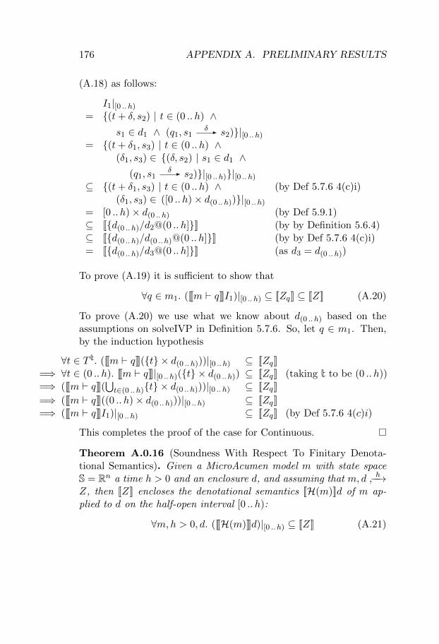
176 APPENDIX A. PRELIMINARY RESULTS
(A.18) as follows:
I1|[0 .. h)= {(t+ δ, s2) | t ∈ (0 .. h) ∧
s1 ∈ d1 ∧ (q1, s1δ- s2)}|[0 .. h)
= {(t+ δ1, s3) | t ∈ (0 .. h) ∧(δ1, s3) ∈ {(δ, s2) | s1 ∈ d1 ∧
(q1, s1δ- s2)}|[0 .. h)}|[0 .. h)
⊆ {(t+ δ1, s3) | t ∈ (0 .. h) ∧ (by Def 5.7.6 4(c)i)(δ1, s3) ∈ ([0 .. h)× d(0 .. h))}|[0 .. h)
= [0 .. h)× d(0 .. h) (by Def 5.9.1)
⊆ [[{d(0 .. h)/d2@(0 .. h]}]] (by by Definition 5.6.4)
⊆ [[{d(0 .. h)/d(0 .. h)@(0 .. h]}]] (by by Def 5.7.6 4(c)i)
= [[{d(0 .. h)/d3@(0 .. h]}]] (as d3 = d(0 .. h))
To prove (A.19) it is sufficient to show that
∀q ∈ m1. ([[[m ` q]]]I1)|[0 .. h) ⊆ [[Zq]] ⊆ [[Z]] (A.20)
To prove (A.20) we use what we know about d(0 .. h) based on theassumptions on solveIVP in Definition 5.7.6. So, let q ∈ m1. Then,by the induction hypothesis
∀t ∈ T t. ([[[m ` q]]]({t} × d(0 .. h)))|[0 .. h) ⊆ [[Zq]]
=⇒ ∀t ∈ (0 .. h). [[[m ` q]]]|[0 .. h)({t} × d(0 .. h)) ⊆ [[Zq]] (taking t to be (0 .. h))
=⇒ ([[[m ` q]]](⋃t∈(0 .. h){t} × d(0 .. h)))|[0 .. h) ⊆ [[Zq]]
=⇒ ([[[m ` q]]]((0 .. h)× d(0 .. h)))|[0 .. h) ⊆ [[Zq]]
=⇒ ([[[m ` q]]]I1)|[0 .. h) ⊆ [[Zq]] (by Def 5.7.6 4(c)i)
This completes the proof of the case for Continuous.
Theorem A.0.16 (Soundness With Respect To Finitary Denota-tional Semantics). Given a MicroAcumen model m with state spaceS = Rn a time h > 0 and an enclosure d, and assuming that m, d h↪−−→Z, then [[Z]] encloses the denotational semantics [[H(m)]]d of m ap-plied to d on the half-open interval [0 .. h):
∀m,h > 0, d. ([[[H(m)]]]d)|[0 .. h) ⊆ [[Z]] (A.21)
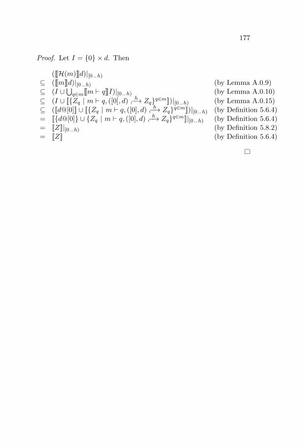
177
Proof. Let I = {0} × d. Then
([[[H(m)]]]d)|[0 .. h)⊆ ([[[m]]]d)|[0 .. h) (by Lemma A.0.9)
⊆ (I ∪⋃q∈m[[[m ` q]]]I)|[0 .. h) (by Lemma A.0.10)
⊆ (I ∪ [[{Zq | m ` q, ([0], d) h↪−→ Zq}q∈m]])|[0 .. h) (by Lemma A.0.15)
⊆ ([[d@[0]]] ∪ [[{Zq | m ` q, ([0], d) h↪−→ Zq}q∈m]])|[0 .. h) (by Definition 5.6.4)
= [[{d@[0]} ∪ {Zq | m ` q, ([0], d) h↪−→ Zq}q∈m]]|[0 .. h) (by Definition 5.6.4)
= [[Z]]|[0 .. h) (by Definition 5.8.2)
= [[Z]] (by Definition 5.6.4)

178 APPENDIX A. PRELIMINARY RESULTS
Appendix B
State Space Power Setsand Closed-Power Sets asLattices
This appendix casts two variants of the power set of state space, thedomain over which the denotational semantics of MicroAcumen isdefined in Section 5.4.4, as a complete lattice. A complete lattice isa structure that consists of a set and an ordering relation, along withcertain requirements on its elements in terms of this relation. Mapsover complete lattices often possess useful properties. Crucially, whena map is monotone, Tarski’s fixpoint theorem [Tar] guarantees thatthe map has a least and a greatest fixpoint. Section 5.4.4 exploits thisfact to define the evolution of a hybrid system as the least fixpoint ofa monotone map.
The appendix is organized as follows. First, the notion of a com-plete lattice is defined. Second, this notion is used to define twoconcrete, complete lattices. The first lattice is over P(Rn), the powerset of the state space, and the second is over Pclosed(Rn), the set ofclosed subsets of the state space. Basically, these are lattices wheresuprema are unions and infima are intersections. However, for P(Rn),the union of an infinite set of closed sets may not be closed. So, forPclosed(Rn), we must define the supremum as the topological closure
179
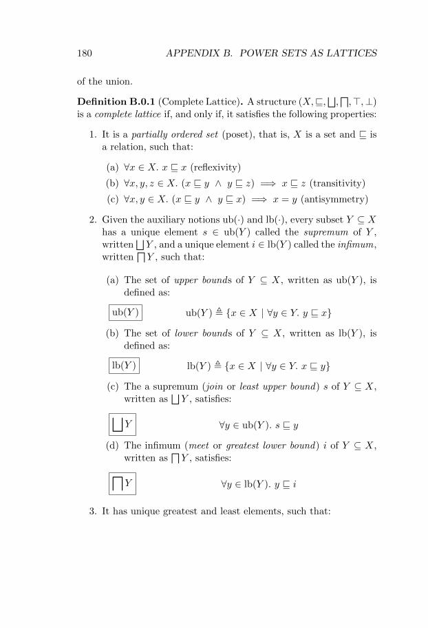
180 APPENDIX B. POWER SETS AS LATTICES
of the union.
Definition B.0.1 (Complete Lattice). A structure (X,v,⊔,d,>,⊥)
is a complete lattice if, and only if, it satisfies the following properties:
1. It is a partially ordered set (poset), that is, X is a set and v isa relation, such that:
(a) ∀x ∈ X. x v x (reflexivity)
(b) ∀x, y, z ∈ X. (x v y ∧ y v z) =⇒ x v z (transitivity)
(c) ∀x, y ∈ X. (x v y ∧ y v x) =⇒ x = y (antisymmetry)
2. Given the auxiliary notions ub(·) and lb(·), every subset Y ⊆ Xhas a unique element s ∈ ub(Y ) called the supremum of Y ,written
⊔Y , and a unique element i ∈ lb(Y ) called the infimum,
writtendY , such that:
(a) The set of upper bounds of Y ⊆ X, written as ub(Y ), isdefined as:
ub(Y ) ub(Y ) , {x ∈ X | ∀y ∈ Y. y v x}
(b) The set of lower bounds of Y ⊆ X, written as lb(Y ), isdefined as:
lb(Y ) lb(Y ) , {x ∈ X | ∀y ∈ Y. x v y}
(c) The a supremum (join or least upper bound) s of Y ⊆ X,written as
⊔Y , satisfies:⊔
Y ∀y ∈ ub(Y ). s v y
(d) The infimum (meet or greatest lower bound) i of Y ⊆ X,written as
dY , satisfies:
lY ∀y ∈ lb(Y ). y v i
3. It has unique greatest and least elements, such that:
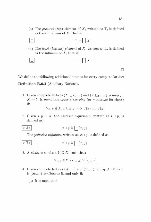
181
(a) The greatest (top) element of X, written as >, is definedas the supremum of X, that is:
> > =⊔X
(b) The least (bottom) element of X, written as ⊥, is definedas the infimum of X, that is:
⊥ ⊥ =lX
�
We define the following additional notions for every complete lattice:
Definition B.0.2 (Auxiliary Notions).
1. Given complete lattices (X,vX , . . .) and (Y,vY , . . .), a map f :X → Y is monotone order preserving (or monotone for short)if:
∀x, y ∈ X. x vX y =⇒ f(x) vY f(y)
2. Given x, y ∈ X, the pairwise supremum, written as x t y, isdefined as:
x t y x t y ,⊔{x, y}
The pairwise infimum, written as x u y, is defined as:
x u y x u y ,l{x, y}
3. A chain is a subset Y ⊆ X, such that:
∀x, y ∈ Y. (x v y) ∨ (y v x)
4. Given complete lattices (X, . . .) and (Y, . . .), a map f : X → Yis (Scott-) continuous if, and only if:
(a) It is monotone
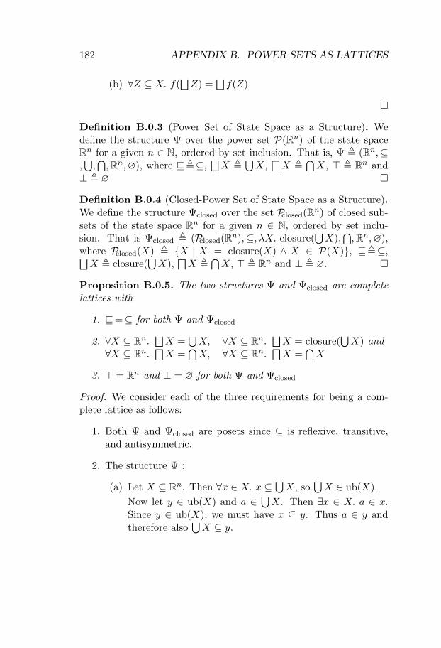
182 APPENDIX B. POWER SETS AS LATTICES
(b) ∀Z ⊆ X. f(⊔Z) =
⊔f(Z)
�
Definition B.0.3 (Power Set of State Space as a Structure). Wedefine the structure Ψ over the power set P(Rn) of the state spaceRn for a given n ∈ N, ordered by set inclusion. That is, Ψ , (Rn,⊆,⋃,⋂,Rn,∅), where v,⊆,
⊔X ,
⋃X,
dX ,
⋂X, > , Rn and
⊥ , ∅ �
Definition B.0.4 (Closed-Power Set of State Space as a Structure).We define the structure Ψclosed over the set Pclosed(Rn) of closed sub-sets of the state space Rn for a given n ∈ N, ordered by set inclu-sion. That is Ψclosed , (Pclosed(Rn),⊆, λX. closure(
⋃X),
⋂,Rn,∅),
where Pclosed(X) , {X | X = closure(X) ∧ X ∈ P(X)}, v,⊆,⊔X , closure(
⋃X),
dX ,
⋂X, > , Rn and ⊥ , ∅. �
Proposition B.0.5. The two structures Ψ and Ψclosed are completelattices with
1. v=⊆ for both Ψ and Ψclosed
2. ∀X ⊆ Rn.⊔X =
⋃X, ∀X ⊆ Rn.
⊔X = closure(
⋃X) and
∀X ⊆ Rn.dX =
⋂X, ∀X ⊆ Rn.
dX =
⋂X
3. > = Rn and ⊥ = ∅ for both Ψ and Ψclosed
Proof. We consider each of the three requirements for being a com-plete lattice as follows:
1. Both Ψ and Ψclosed are posets since ⊆ is reflexive, transitive,and antisymmetric.
2. The structure Ψ :
(a) Let X ⊆ Rn. Then ∀x ∈ X. x ⊆⋃X, so
⋃X ∈ ub(X).
Now let y ∈ ub(X) and a ∈⋃X. Then ∃x ∈ X. a ∈ x.
Since y ∈ ub(X), we must have x ⊆ y. Thus a ∈ y andtherefore also
⋃X ⊆ y.
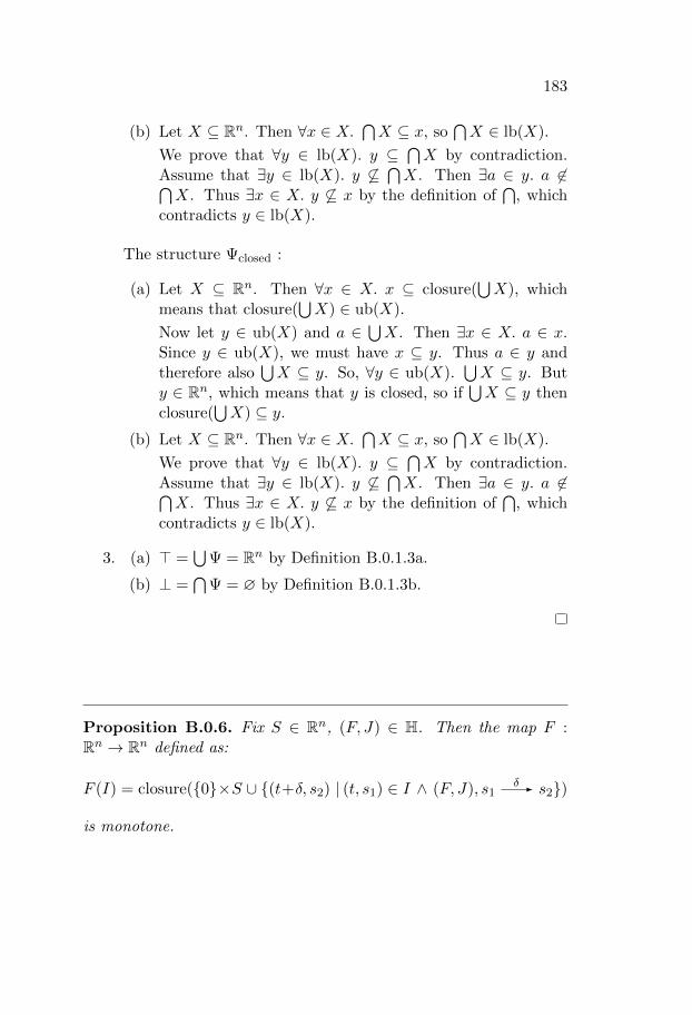
183
(b) Let X ⊆ Rn. Then ∀x ∈ X.⋂X ⊆ x, so
⋂X ∈ lb(X).
We prove that ∀y ∈ lb(X). y ⊆⋂X by contradiction.
Assume that ∃y ∈ lb(X). y 6⊆⋂X. Then ∃a ∈ y. a 6∈⋂
X. Thus ∃x ∈ X. y 6⊆ x by the definition of⋂
, whichcontradicts y ∈ lb(X).
The structure Ψclosed :
(a) Let X ⊆ Rn. Then ∀x ∈ X. x ⊆ closure(⋃X), which
means that closure(⋃X) ∈ ub(X).
Now let y ∈ ub(X) and a ∈⋃X. Then ∃x ∈ X. a ∈ x.
Since y ∈ ub(X), we must have x ⊆ y. Thus a ∈ y andtherefore also
⋃X ⊆ y. So, ∀y ∈ ub(X).
⋃X ⊆ y. But
y ∈ Rn, which means that y is closed, so if⋃X ⊆ y then
closure(⋃X) ⊆ y.
(b) Let X ⊆ Rn. Then ∀x ∈ X.⋂X ⊆ x, so
⋂X ∈ lb(X).
We prove that ∀y ∈ lb(X). y ⊆⋂X by contradiction.
Assume that ∃y ∈ lb(X). y 6⊆⋂X. Then ∃a ∈ y. a 6∈⋂
X. Thus ∃x ∈ X. y 6⊆ x by the definition of⋂
, whichcontradicts y ∈ lb(X).
3. (a) > =⋃
Ψ = Rn by Definition B.0.1.3a.
(b) ⊥ =⋂
Ψ = ∅ by Definition B.0.1.3b.
Proposition B.0.6. Fix S ∈ Rn, (F, J) ∈ H. Then the map F :Rn → Rn defined as:
F (I) = closure({0}×S ∪ {(t+δ, s2) | (t, s1) ∈ I ∧ (F, J), s1δ- s2})
is monotone.
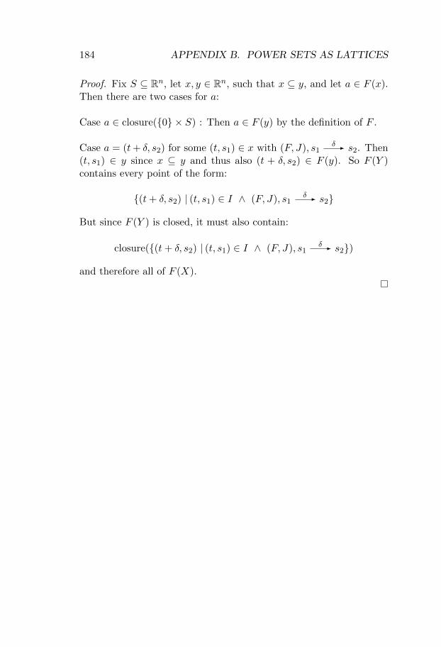
184 APPENDIX B. POWER SETS AS LATTICES
Proof. Fix S ⊆ Rn, let x, y ∈ Rn, such that x ⊆ y, and let a ∈ F (x).Then there are two cases for a:
Case a ∈ closure({0} × S) : Then a ∈ F (y) by the definition of F .
Case a = (t+ δ, s2) for some (t, s1) ∈ x with (F, J), s1δ- s2. Then
(t, s1) ∈ y since x ⊆ y and thus also (t + δ, s2) ∈ F (y). So F (Y )contains every point of the form:
{(t+ δ, s2) | (t, s1) ∈ I ∧ (F, J), s1δ- s2}
But since F (Y ) is closed, it must also contain:
closure({(t+ δ, s2) | (t, s1) ∈ I ∧ (F, J), s1δ- s2})
and therefore all of F (X).
Bibliography
[A+1] Matthias Althoff et al. Reachability analysis and its ap-plication to the safety assessment of autonomous cars.Technische Universitt Munchen, 2010.
[A+2] Kevin Atkinson et al. GNU aspell. http://aspell.net,2016.
[Acu] Acumen. http://acumen-language.org, 2016.
[ADI] Rajeev Alur, Thao Dang, and Franjo Ivancic. Progresson reachability analysis of hybrid systems using predicateabstraction. In International Workshop on Hybrid Sys-tems: Computation and Control, pages 4–19. Springer,2003.
[AGH] Ken Arnold, James Gosling, and David Holmes. The Javaprogramming language, volume 2. Addison-Wesley Read-ing, 2000.
[AHS] Jirı Adamek, Horst Herrlich, and George E Strecker. Ab-stract and concrete categories. The joy of cats. Citeseer,2004.
[ALM] Polarion ALM. http://polarion.com, 2016.
[aR] Acumen 2016 08 30 Release. https://bitbucket.
org/effective/acumen-dev/downloads/2016_08_30_
Acumen.zip, 2016.
185
186 BIBLIOGRAPHY
[ASK] Aditya Agrawal, Gyula Simon, and Gabor Karsai. Se-mantic translation of Simulink/Stateflow models to hy-brid automata using graph transformations. ElectronicNotes in Theoretical Computer Science, 109:43–56, 2004.
[AvBR] DE Nadales Agut, Dirk A van Beek, and JE Rooda. Syn-tax and semantics of the compositional interchange for-mat for hybrid systems. The Journal of Logic and Alge-braic Programming, 82(1):1–52, 2013.
[AZD+] Ayman Aljarbouh, Yingfu Zeng, Adam Duracz, BenoıtCaillaud, and Walid Taha. Chattering-free simulation forhybrid dynamical systems. In 2016 IEEE InternationalConference on Computational Science and Engineering,IEEE International Conference on Embedded and Ubiq-uitous Computing, and International Symposium on Dis-tributed Computing and Applications to Business, Engi-neering and Science. IEEE Computer Society, 2016.
[Bar] Ferenc A. Bartha. Computer-aided proofs and algorithmsin analysis. PhD thesis, The University of Bergen, 2013.
[BC] Olivier Bouissou and Alexandre Chapoutot. An opera-tional semantics for simulink’s simulation engine. ACMSIGPLAN Notices, 47(5):129–138, 2012.
[BF] Simon Bliudze and Sebastien Furic. An operational se-mantics for hybrid systems involving behavioral abstrac-tion. In Proceedings of the 10 th International Model-ica Conference; March 10-12; 2014; Lund; Sweden, num-ber 096 in Linkoping Electronic Conference Proceedings,pages 693–706. Linkoping University Electronic Press,2014.
[Ble] Blender Online Community. Blender - a 3D modellingand rendering package. Blender Foundation, Blender In-stitute, Amsterdam, 2016.
BIBLIOGRAPHY 187
[BM] Olivier Bouissou and Matthieu Martel. Grklib: a guaran-teed Runge Kutta library. In Scientific Computing, Com-puter Arithmetic and Validated Numerics, 2006. SCAN2006. 12th GAMM-IMACS International Symposium on,pages 8–8, Washington, DC, USA, 2006. IEEE, IEEEComputer Society.
[BMAHA] Youssef A Bazzi, Mohannad Murad, Nizar Al-Holou, andRawa Adla. Automotive collision avoidance methodolo-gies sensor-based and its-based. In 2013 ACS Interna-tional Conference on Computer Systems and Applications(AICCSA), pages 1–8. IEEE, 2013.
[Bro] David Broman. Meta-Languages and Semantics forEquation-Based Modeling and Simulation. PhD thesis,Linkoping University, 2010.
[BT] Paul Brauner and Walid Mohamed Taha. Globallyparallel, locally sequential: a preliminary proposal foracumen objects. In Proceedings of the 9th Workshopon Parallel/High-Performance Object-Oriented ScientificComputing, page 2. ACM, 2010.
[BTR] Fadi Basma, Yehia Tachwali, and Hazem H Refai. In-tersection collision avoidance system using infrastructurecommunication. In Intelligent Transportation Systems(ITSC), 2011 14th International IEEE Conference on,pages 422–427, Washington, DC, 2011. IEEE.
[CAP] CAPD - Computer Assisted Proofs in Dynamics group,a C++ package for rigorous numerics. http://capd.
wsb-nlu.edu.pl, 2016.
[CAS] Xin Chen, Erika Abraham, and Sriram Sankara-narayanan. Flow*: An analyzer for non-linear hybridsystems. In International Conference on Computer AidedVerification, pages 258–263. Springer, 2013.
188 BIBLIOGRAPHY
[CB] Ching-Yao Chan and Benedicte Bougler. Evaluation ofcooperative roadside and vehicle-based data collectionfor assessing intersection conflicts. In Intelligent Vehi-cles Symposium, 2005. Proceedings, pages 165–170. IEEE,2005.
[CEB] Erik Coelingh, Andreas Eidehall, and Mattias Bengts-son. Collision warning with full auto brake and pedestriandetection-a practical example of automatic emergencybraking. In Intelligent Transportation Systems (ITSC),2010 13th International IEEE Conference on, pages 155–160. IEEE, 2010.
[CH] Koen Claessen and John Hughes. QuickCheck: alightweight tool for random testing of Haskell programs.Acm sigplan notices, 46(4):53–64, 2011.
[Che] Xin Chen. Reachability Analysis of Non-Linear HybridSystems Using Taylor Models. PhD thesis, Ph. D. thesis,RWTH Aachen University, Germany, 2015.
[Cho] Eun-Ha Choi. Crash factors in intersection-relatedcrashes: An on-scene perspective. Technical report, Na-tional Highway Traffic Safety Administration, 2010.
[CJ] G. Chabert and L. Jaulin. Contractor Programming. Ar-tificial Intelligence, 173:1079–1100, 2009.
[CPPSV] Luca P Carloni, Roberto Passerone, Alessandro Pinto,and Alberto Sangiovanni-Vincentelli. Languages and toolsfor hybrid systems design. now Publishers Inc, 2006.
[DBT] Adam Duracz, Ferenc A. Bartha, and Walid Taha. Ac-curate rigorous simulation should be possible for gooddesigns. In 2016 International Workshop on Symbolicand Numerical Methods for Reachability Analysis (SNR),pages 1–10, April 2016.
BIBLIOGRAPHY 189
[DEB+] Adam Duracz, Henrik Eriksson, Ferenc A. Bartha, YingfuZeng, Fei Xu, and Walid Taha. Using rigorous simulationto support ISO 26262 hazard analysis and risk assess-ment. In 2015 IEEE 12th International Conference onEmbedded Software and Systems (ICESS), pages 1093–1096. IEEE, August 2015.
[DFKT] Jan Duracz, Amin Farjudian, Michal Konecny, and WalidTaha. Function interval arithmetic. In MathematicalSoftware–ICMS 2014, pages 677–684. Springer, 2014.
[DFS] Luiz Henrique De Figueiredo and Jorge Stolfi. Affinearithmetic: concepts and applications. Numerical Algo-rithms, 37(1-4):147–158, 2004.
[EH] Conal Elliott and Paul Hudak. Functional reactive ani-mation. ACM SIGPLAN Notices, 32(8):263–273, 1997.
[EP] Abbas Edalat and Dirk Pattinson. Denotational seman-tics of hybrid automata. The Journal of Logic and Alge-braic Programming, 73(1):3–21, 2007.
[EU] EU. Regulation no 347/2012. Type-Approval Require-ments for Certain Categories of Motor Vehicles with Re-gard to Advanced emergency Braking Systems, 2012.
[FLGD+] Goran Frehse, Colas Le Guernic, Alexandre Donze, ScottCotton, Rajarshi Ray, Olivier Lebeltel, Rodolfo Ripado,Antoine Girard, Thao Dang, and Oded Maler. SpaceEx:Scalable verification of hybrid systems. In InternationalConference on Computer Aided Verification, pages 379–395. Springer, 2011.
[Fri] Peter Fritzson. Principles of object-oriented modeling andsimulation with Modelica 3.3: a cyber-physical approach.John Wiley & Sons, 2014.
[Gao] Sicun Gao. Computable Analysis, Decision Procedures,and Hybrid Automata: A New Framework for the Formal
190 BIBLIOGRAPHY
Verification of Cyber-Physical Systems. PhD thesis, PhDthesis, Carnegie Mellon University, 2012.
[GI] Alexandre Goldsztejn and Daisuke Ishii. A parallelotopemethod for hybrid system simulation. Reliable Comput-ing, 23:163–185, 2016.
[GST] Rafal Goebel, Ricardo G Sanfelice, and Andrew R Teel.Hybrid Dynamical Systems: modeling, stability, and ro-bustness. Princeton University Press, 2012.
[HBG+] Alan C Hindmarsh, Peter N Brown, Keith E Grant,Steven L Lee, Radu Serban, Dan E Shumaker, andCarol S Woodward. SUNDIALS: Suite of nonlinear anddifferential/algebraic equation solvers. ACM Transac-tions on Mathematical Software (TOMS), 31(3):363–396,2005.
[Hen] T. A. Henzinger. The theory of hybrid automata. In Logicin Computer Science, pages 278–292, New Brunswick, NJ,1996. IEEE Computer Society.
[HHHK] Ernst Moritz Hahn, Arnd Hartmanns, Holger Hermanns,and Joost-Pieter Katoen. A compositional modelling andanalysis framework for stochastic hybrid systems. FormalMethods in System Design, 2012. ISSN: 0925-9856.
[HT] Nicholas Hale and Lloyd N Trefethen. Chebfun andnumerical quadrature. Science China Mathematics,55(9):1749–1760, 2012.
[IEE] IEEE. Standard for Floating-Point Arithmetic. Std 754-2008, pages 1–70, August 2008.
[ILO] SA ILOG. Revising hull and box consistency. In LogicProgramming: Proceedings of the 1999 International Con-ference on Logic Programming, page 230. MIT press,1999.
BIBLIOGRAPHY 191
[Ish] Daisuke Ishii. Simulation and verification of hybrid sys-tems based on interval analysis and constraint program-ming. PhD thesis, School of Science and Engineering,Waseda University, 2010.
[ISO] ISO26262. Road vehicles – functional safety, 2011.
[JM] Taylor T Johnson and Sayan Mitra. Parametrized verifi-cation of distributed cyber-physical systems: An aircraftlanding protocol case study. In Proceedings of the 2012IEEE/ACM Third International Conference on Cyber-Physical Systems, pages 161–170. IEEE Computer Soci-ety, 2012.
[KDFT] Michal Konecny, Jan Duracz, Amin Farjudian, and WalidTaha. Picard method for enclosing ODEs with uncertaininitial values. In 11th International Conference on Com-putability and Complexity in Analysis, pages 41–42, 2014.
[KTB+] Michal Konecny, Walid Taha, Ferenc A. Bartha, JanDuracz, Adam Duracz, and Aaron D Ames. Enclosingthe behavior of a hybrid automaton up to and beyond aZeno point. Nonlinear Analysis: Hybrid Systems, 20:1–20, 2016.
[LFBZ] Long Le, Andreas Festag, Roberto Baldessari, and Wen-hui Zhang. V2x communication and intersection safety.In Advanced Microsystems for Automotive Applications2009, pages 97–107. Springer, 2009.
[LML] Xiaojun Liu, Eleftherios Matsikoudis, and Edward A Lee.Modeling timed concurrent systems. In Concurrency The-ory, pages 1–15. Springer, 2006.
[Loh] Rudolf J. Lohner. AWA. Software product in FORTRAN-SC for the inclusion of the solution of ODEs, Karlsruhe,1989.
192 BIBLIOGRAPHY
[LPN] Sarah M Loos, Andre Platzer, and Ligia Nistor. Adap-tive cruise control: Hybrid, distributed, and now formallyverified. In FM 2011: Formal Methods, pages 42–56.Springer, 2011.
[LSV] Nancy Lynch, Roberto Segala, and Frits Vaandrager.Hybrid i/o automata. Information and Computation,185(1):105 – 157, 2003.
[Mat1] Mathematica 10.0, Wolfram Research, Inc. https://
www.wolfram.com, 2016.
[MAT2] MATLAB. version 9.0 (R2016a). The MathWorks Inc.,Natick, Massachusetts, 2016.
[MB1] Kyoko Makino and Martin Berz. Taylor models andother validated functional inclusion methods. Interna-tional Journal of Pure and Applied Mathematics, 4,4,2003.
[MB2] Ramon E. Moore and Fritz Bierbaum. Methods and ap-plications of interval analysis, volume 2. SIAM, 1979.
[MCD+] James A Misener, Ching-Yao Chan, Susan Dickey, Zu-Whan Kim, Tom Kuhn, Thang Lian, David Nelson,Ashkan Sharafsaleh, Steven Shladover, John Spring, JoelVanderWerf, Wei-Bin Zhang, Liping Zhang, and KunZhou. Cooperative intersection collision avoidance system(cicas): Signalized left turn assist and traffic signal adap-tation. Technical Report UCB-ITS-PRR-2010-20, Uni-versity of California, Berkeley, 2010.
[med] medini analyze. http://www.medini.eu, 2016.
[MF] Stefano Minopoli and Goran Frehse. Sl2sx translator:From simulink to spaceex models. In Proceedings of the19th International Conference on Hybrid Systems: Com-putation and Control, pages 93–98. ACM, 2016.
BIBLIOGRAPHY 193
[MMP] Oded Maler, Zohar Manna, and Amir Pnueli. From timedto hybrid systems. In Real-time: theory in practice, pages447–484. Springer, 1992.
[Moo] Ramon E. Moore. Interval analysis, volume 4. Prentice-Hall Englewood Cliffs, 1966.
[MPD+] Jawad Masood, Roland Philippsen, Jan Duracz, WalidTaha, Henrik Eriksson, and Christian Grante. Domainanalysis for standardised functional safety: a case studyon design-time verification of automatic emergency brak-ing. In International Federation of Automotive Engineer-ing Societies 2014 World Automotive Congress, Maas-tricht, The Netherlands, 2-6 June, 2014. FISITA, 2014.
[MS] Ammar Mohammed and Frieder Stolzenburg. Implement-ing hierarchical hybrid automata using constraint logicprogramming. In Proceedings of 22nd Workshop on (Con-straint) Logic Programming, Dresden, pages 60–71. Cite-seer, 2008.
[MU] Shota Matsumoto and Kazunori Ueda. Hyrose. ComputerSoftware, 30(4):18–35, 2013.
[Ned] Nedialko S Nedialkov. Interval tools for ODEs and DAEs.In Scientific Computing, Computer Arithmetic and Vali-dated Numerics, 2006. SCAN 2006. 12th GAMM-IMACSInternational Symposium on, pages 4–4. IEEE, 2006.
[NJC] Nedialko S Nedialkov, Kenneth R Jackson, and George FCorliss. Validated solutions of initial value problems forordinary differential equations. Applied Mathematics andComputation, 105(1):21–68, 1999.
[NPT] Nedialko S Nedialkov, John D Pryce, and GuangningTan. Algorithm 948: DAESA—A Matlab tool for struc-tural analysis of differential-algebraic equations: Soft-ware. ACM Transactions on Mathematical Software(TOMS), 41(2):12, 2015.
194 BIBLIOGRAPHY
[NRS] Pablo Nanez, Nathalie Risso, and Ricardo G Sanfelice. Asymbolic simulator for hybrid equations. In Proceedingsof the 2014 Summer Simulation Multiconference, page 18.Society for Computer Simulation International, 2014.
[NZ] Dmitry Yu Nadezhin and Sergei I Zhilin. JInterval Li-brary: Principles, Development, and Perspectives. Reli-able Computing, 19(3):229–247, 2013.
[Oa] Martin Odersky and al. An Overview of the ScalaProgramming Language. Technical Report IC/2004/64,EPFL, Lausanne, Switzerland, 2004.
[PA] Amadeusz Pawlik and Henry Andersson. Visualisinginterval-based simulations, 2015.
[PC] Andre Platzer and Edmund M Clarke. Formal verificationof curved flight collision avoidance maneuvers: A casestudy. Springer, 2009.
[Pla1] Andre Platzer. Differential dynamic logic for hybrid sys-tems. Journal of Automated Reasoning, 41(2):143–189,2008.
[Pla2] Andre Platzer. Quantified differential dynamic logic fordistributed hybrid systems. In International Workshop onComputer Science Logic, pages 469–483. Springer, 2010.
[PQ] Andre Platzer and Jan-David Quesel. KeYmaera: A hy-brid theorem prover for hybrid systems (system descrip-tion). In International Joint Conference on AutomatedReasoning, pages 171–178. Springer, 2008.
[Ral] LB Rall. Differentiation arithmetics. Computer arith-metic and self-validating numerical methods, pages 73–90,1990.
[Red] Felix Redmill. Understanding the use, misuse and abuseof safety integrity levels. In Proceedings of the Eighth
BIBLIOGRAPHY 195
Safety-critical Systems Symposium, pages 8–10. Citeseer,2000.
[Rep] Acumen Source Code Repository. https://bitbucket.
org/effective/acumen-dev, 2016.
[RG] Rajarshi Ray and Amit Gurung. Parallel state space ex-ploration of linear systems with inputs using XSpeed. InProceedings of the 18th International Conference on Hy-brid Systems: Computation and Control, pages 285–286.ACM, 2015.
[Ris] RiskCAT. http://www.hitex.co.uk, 2016.
[RS] Stefan Ratschan and Zhikun She. Safety verification ofhybrid systems by constraint propagation based abstrac-tion refinement. ACM Transactions in Embedded Com-puting Systems, 6(1), 2007.
[RSy] RSyntaxTextArea. http://bobbylight.github.io/
RSyntaxTextArea, 2016.
[SBN+] Janos Sztipanovits, Ted Bapty, Sandeep Neema, LarryHoward, and Ethan Jackson. OpenMETA: A model-and component-based design tool chain for cyber-physicalsystems. In Joint European Conferences on Theory andPractice of Software, pages 235–248. Springer, 2014.
[Sca] ScalaCheck. https://www.scalacheck.org, 2016.
[SOX] SOX2. http://enco-software.com, 2016.
[SRKC] B Izaias Silva, Keith Richeson, Bruce Krogh, andAlongkrit Chutinan. Modeling and verifying hybrid dy-namic systems using checkmate. In Proceedings of 4thInternational Conference on Automation of Mixed Pro-cesses, volume 4, pages 1–7. Citeseer, 2000.
196 BIBLIOGRAPHY
[Sun] Teruo Sunaga. Theory of an interval algebra and its ap-plication to numerical analysis [reprint of res. assoc. appl.geom. mem. 2 (1958), 29–46]. Japan Journal of Industrialand Applied Mathematics, 26(2-3):125–143, 10 2009.
[Tar] Alfred Tarski. A lattice-theoretical fixpoint theoremand its applications. Pacific Journal of Mathematics,5(2):285–309, 1955.
[TCPZ1] Walid Taha, Robert Cartwright, Roland Philippsen, andYingfu Zeng. Experiences with a first course on cyber-physical systems. In Proceedings of WESE workshop,2013.
[TCPZ2] Walid Taha, Robert Cartwright, Roland Philippsen, andYingfu Zeng. A first course on cyber physical systems. InWorkshop on Cyber-Physical Systems Education (CPS-Ed), 2013.
[TCPZ3] Walid Taha, Robert Cartwright, Roland Philippsen, andYingfu Zeng. Developing a first course on cyber-physicalsystems. In Proceedings of the WESE’14: Workshop onEmbedded and Cyber-Physical Systems Education, page 6.ACM, 2014.
[TDZ+] Walid Taha, Adam Duracz, Yingfu Zeng, Kevin Atkin-son, Ferenc A. Bartha, Paul Brauner, Jan Duracz, FeiXu, Robert Cartwright, Michal Konecny, Eugenio Moggi,Jawad Masood, Pererik Andreasson, Jun Inoue, AnitaSant’Anna, Roland Philippsen, Alexandre Chapoutot,Marcia O’Malley, Aaron Ames, Veronica Gaspes, LiseHvatum, Shyam Mehta, Henrik Eriksson, and ChristianGrante. Acumen: An open-source testbed for cyber-physical systems research. In Proceedings of EAI Interna-tional Conference on CYber physiCaL systems, iOt andsensors Networks (CYCLONE), 2015. EAI, 2015.
BIBLIOGRAPHY 197
[TGP] Walid Taha, Veronica Gaspes, and Rex Page. Accurateprogramming: Thinking about programs in terms of prop-erties. arXiv preprint arXiv:1109.0786, 2011.
[THX+] Walid Taha, Lars-Goran Hedstrom, Fei Xu, Adam Du-racz, Ferenc A. Bartha, Yingfu Zeng, Jennifer David,and Gaurav Gunjan. Flipping a first course on cyber-physical systems–an experience report. In Workshop onEmbedded and Cyber-Physical Systems Education (WESE2016), Pittsburgh, PA, USA, 2016.
[Tiw] A. Tiwari. Formal semantics and analysis methods forSimulink Stateflow models. Technical report, SRI Inter-national, 2002. http://www.csl.sri.com/∼tiwari/-stateflow.html.
[Tuc] Warwick Tucker. Validated numerics: a short intro-duction to rigorous computations. Princeton UniversityPress, 2011.
[UMT+] Kazunori Ueda, Shota Matsumoto, Akira Takeguchi, Hi-roshi Hosobe, Daisuke Ishii, et al. HydLa: A High-LevelLanguage for Hybrid Systems. In Proc. Second Workshopon Logics for System Analysis, pages 3–17. Citeseer, 2012.
[War] Mieczys law Warmus. Calculus of approximations. Bul-letin de L’Academie Polonaise des Sciences, Cl. III,IV(5):253–259, 1956.
[WBWB+] Anna Wrige Berling, Krister Wolff, Fredrik Bruzelius,John Lang, Anders Odblom, Henrik Eriksson, andVivetha Natterjee. Final report: Next generation testmethods, March 2015.
[WH] Zhanyong Wan and Paul Hudak. Functional reactive pro-gramming from first principles. ACM SIGPLAN Notices,35(5):242–252, 2000.
198 BIBLIOGRAPHY
[Xu] Fei Xu. Lightweight Immersion Techniques for Acumen.Master’s thesis, Halmstad University, 2015.
[Zen] Yingfu Zeng. Lightweight three-dimensional visualizationfor hybrid systems simulation. Master’s thesis, HalmstadUniversity, 2012.
[ZRT+] Yingfu Zeng, Chad Rose, Walid Taha, Adam Duracz,Kevin Atkinson, Roland Philippsen, Robert Cartwright,and Marcia O’Malley. Modeling electromechanical as-pects of cyber-physical systems. Journal of Software En-gineering for Robotics, Special Issue on Domain-SpecificLanguages and Models for Robotic Systems, 2016.
[ZWI+] Yun Zhu, Edwin Westbrook, Jun Inoue, AlexandreChapoutot, Cherif Salama, Marisa Peralta, Travis Mar-tin, Walid Taha, Marcia O’Malley, Robert Cartwright,et al. Mathematical equations as executable mod-els of mechanical systems. In Proceedings of the 1stACM/IEEE International Conference on Cyber-PhysicalSystems, pages 1–11. ACM, 2010.
Glossary
AEBS Advanced Emergency Braking System. 117, 118, 120
ASIL Automotive Safety Integrity Level. 116, 117
AST Abstract Syntax Tree. 106, 155
BNF Backus-Naur Form. 52, 55, 63, 79
CBD Critical Braking Distance. 118
CLI Command Line Interface. 99
CPS Cyber-Physical Systems. 21, 29, 39, 40
CWD Critical Warning Distance. 118
DAE Differential-Algebraic Equation. 30, 31, 33, 35, 157, 158
DDE Delay Differential Equation. 31
dL Differential Dynamic Logic. 32
DSL Domain-Specific Language. 39
DSP Digital Signal Processing. 140
FIR Finite Impulse Response. 140, 144
199
200 Glossary
FRP Functional Reactive Programming. 39
GUI Graphical User Interface. 99, 100, 101
HARA Hazard Analysis and Risk Assessment. 116, 117
ICAS Intersection Collision Avoidance System. 15, 117, 118, 121,122
IVP Initial Value Problem. 77, 83, 88, 98, 111
NG-TEST Next Generation Test Methods for Active Safety Func-tions. 117, 118
ODE Ordinary Differential Equation. 35, 83, 88, 98, 111
TTC Time-To-Collision. 118, 121
Index
Simulink, 32
Stateflow, 32
acausal, 33
activated, 83
active equations, 107
approximations, 22
auxiliary function, 80
block diagrams, 32
Booleans with the trivial topol-ogy, 72
bottom, 181
bounded model checking, 37
chain, 181
children, 43
closed, 71
closure, 71
complement, 71
complete lattice, 180
continuous, 181
continuous modes, 55
delay differential equation, 31
differential equation, 29
differential-algebraic equa-tions, 31
discrete modes, 55discrete states, 31
enclosure interpreter, 104enclosure semantics, 104end-time enclosure, 83event detection, 35event handling, 35events, 35evolution, 77
field, 30field expression, 70flow relation, 75formal verification, 36
greatest element, 181greatest lower bound, 180guard, 55guards, 31
hazard, 116hom-set, 72hybrid automata, 31hybrid system, 29
201
202 INDEX
infimum, 180integrator, 35interval box contractor, 111invariant, 31isotone, 82
join, 180jump relation, 75
lattice, 180least element, 181least upper bound, 180locations, 31lower bound, 180
mathematical models, 22meet, 180model checking, 36Modelica, 33modes, 31monotone, 181monotone order preserving,
181
numerical integrators, 35numerical primitive, 80
open intervals, 71open set, 71over-approximations, 106
pairwise infimum, 181pairwise supremum, 181parent, 43partially ordered set, 180path condition, 53, 56Picard iterator, 111
poset, 180
property, 36
range, 90
range enclosure, 83
reachability, 36
real numbers with the standardtopology, 71
rigorous simulation, 23, 36
risk, 116
safety integrity level, 117
safety property, 115
Scott-continuous, 181
signals, 33
simulation, 34
simulation trace, 35
solution, 77
solver, 35
stateflow charts, 32
supremum, 180
tactics, 37
testing, 36
theorem proving, 36
time step, 35, 79
timed enclosure, 78
top, 181
topological closure, 71
topological space, 71, 73
topology, 71
traditional semantics, 98, 104
trajectory, 35
transition relation, 76
upper bound, 180

INDEX 203
validated numerical integra-tors, 35
validated numerics, 36
value enclosure, 78verification, 34