Risk-Aware Limited Lookahead Control for DynamicResource Provisioning in Enterprise Computing

Systems

Dara Kusic and Nagarajan KandasamyDepartment of Electrical and Computer Engineering

Drexel UniversityPhiladelphia, PA, 19104, USA

kusic@drexel.edu, kandasamy@ece.drexel.edu

November 27, 2006

Abstract

Utility or on-demand computing, a provisioning model where a service provider makescomputing infrastructure available to customers as needed, is becoming increasingly commonin enterprise computing systems. Realizing this model requires making dynamic, and some-times risky, resource provisioning and allocation decisions in an uncertain operating environ-ment to maximize revenue while reducing operating cost. This paper develops an optimizationframework wherein the resource provisioning problem is posed as one of sequential decisionmaking under uncertainty and solved using a limited lookahead control scheme. The proposedapproach accounts for the switching costs incurred during resource provisioning and explicitlyencodes risk in the optimization problem. Simulations using workload traces from the SoccerWorld Cup 1998 web site show that a computing system managed by our controller generatesup to 20% more profit than a system without dynamic control while incurring low control over-head.

Key words: Utility computing, resource provisioning, sequential optimization, limited looka-head control

1 Introduction

Utility computing is an emerging provisioning model where a service provider makes computing

resources available to the customer as needed, and charges them for specific usage rather than a

flat rate. It is becoming increasingly common in enterprise computing, and is sometimes used

for the consumer market as well as Internet services, Web site access and file sharing. Realizing

the utility computing model requires making resource provisioning and allocation decisions in a

1

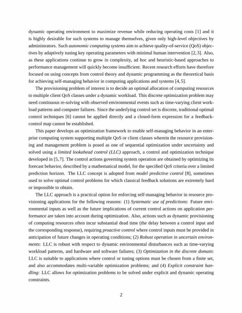
dynamic operating environment to maximize revenue while reducing operating costs [1] and it

is highly desirable for such systems to manage themselves, given only high-level objectives by

administrators. Suchautonomic computing systemsaim to achieve quality-of-service (QoS) objec-

tives by adaptively tuning key operating parameters with minimal human intervention [2,3]. Also,

as these applications continue to grow in complexity, ad hoc and heuristic-based approaches to

performance management will quickly become insufficient. Recent research efforts have therefore

focused on using concepts from control theory and dynamic programming as the theoretical basis

for achieving self-managing behavior in computing applications and systems [4,5].

The provisioning problem of interest is to decide an optimal allocation of computing resources

to multiple client QoS classes under a dynamic workload. This discrete optimization problem may

need continuous re-solving with observed environmental events such as time-varying client work-

load patterns and computer failures. Since the underlying control set is discrete, traditional optimal

control techniques [6] cannot be applied directly and a closed-form expression for a feedback-

control map cannot be established.

This paper develops an optimization framework to enable self-managing behavior in an enter-

prise computing system supporting multiple QoS or client classes wherein the resource provision-

ing and management problem is posed as one of sequential optimization under uncertainty and

solved using alimited lookahead control (LLC)approach, a control and optimization technique

developed in [5,7]. The control actions governing system operation are obtained by optimizing its

forecast behavior, described by a mathematical model, for the specified QoS criteria over a limited

prediction horizon. The LLC concept is adopted frommodel predictive control[8], sometimes

used to solve optimal control problems for which classical feedback solutions are extremely hard

or impossible to obtain.

The LLC approach is a practical option for enforcing self-managing behavior in resource pro-

visioning applications for the following reasons: (1)Systematic use of predictions: Future envi-

ronmental inputs as well as the future implications of current control actions on application per-

formance are taken into account during optimization. Also, actions such as dynamic provisioning

of computing resources often incur substantial dead time (the delay between a control input and

the corresponding response), requiringproactive controlwhere control inputs must be provided in

anticipation of future changes in operating conditions; (2)Robust operation in uncertain environ-

ments: LLC is robust with respect to dynamic environmental disturbances such as time-varying

workload patterns, and hardware and software failures; (3)Optimization in the discrete domain:

LLC is suitable to applications where control or tuning options must be chosen from a finite set,

and also accommodates multi-variable optimization problems; and (4)Explicit constraint han-

dling: LLC allows for optimization problems to be solved under explicit and dynamic operating

constraints.

2

The resource provisioning problem addressed in this paper assumes a computing system sup-

porting three QoS classes using dedicated server clusters for each, dispatching incoming client traf-

fic to the appropriate cluster. To maximize the profit generated by this system under a time-varying

workload, the controller must solve a discrete and dynamic optimization problem to decide: (1)

the number of computers to provision per service cluster, (2) the operating frequency at which to

operate the servers in a cluster and (3) the number of computers to power down to reduce energy

consumption. This paper builds on the LLC framework developed in [5] to solve the above pro-

visioning problem in an uncertain and dynamic operating environment, and makes the following

innovative contributions:

• The profit maximization problem is solved for multiple client classes whose service-level

agreements (SLAs) follow a non-linear pricing strategy.

• Workload forecasting errors and inaccuracies are explicitly discounted along the lookahead

horizon to diminish their effect on control performance.

• The LLC problem formulation models the various switching costs associated with provision-

ing decisions. Revenue may be lost while a computer is being switched between clients, if,

for example, the corresponding computer will be unavailable for some time duration while

a different operating system and/or application is loaded to service the new client. Other

switching costs include the time delay incurred when powering up an idle computer and the

excess energy consumed during this transient phase.

• In an operating environment where the incoming workload is noisy and highly variable,

switching computers excessively between clusters may actually reduce the profit generated,

especially in the presence of the switching costs described above. Thus, each provision-

ing decision made by the controller is risky and we explicitly encode risk in the problem

formulation using preference functions to order possible controller decisions.

Simulations using workload traces from the France World Cup 1998 (WC98) web site [9] show

that a computing system, managed using the proposed LLC method, generates up to 20% more

profit per day when compared to a system operating without dynamic control, and with very low

control overhead. We also characterize the effects of varying key controller parameters such as the

prediction horizon and the risk preference function on its performance.

The paper is organized as follows. Section 2 discusses related work while Section 3 describes

system modeling assumptions and the basic LLC concepts. Section 4 formulates the resource pro-

visioning problem, Section 5 describes the controller design and Section 6 presents experimental

results evaluating controller performance. We conclude the paper in Section 7 with a discussion

on future work.

3

2 Related Work

We now briefly review prior research addressing resource provisioning problems in utility com-

puting models. In [10], a homogeneous computing cluster is operated energy efficiently using

both predictive and reactive resource management techniques. Processors are provisioned using

predicted workload patterns, and a feedback controller sets their aggregate operating frequency,

reacting to short-term workload variations. The system model includes switching costs incurred

when powering computers on and off. Resource provisioning in a multi-tier web environment is

addressed in [11] while [12] develops a controller to allocate a finite number of resources among

multiple applications to maximize a user-defined utility for the entire system. A reactive tech-

nique is proposed in [13] to allocate resources among multiple client classes, balance the load

across servers, and handle dynamic fluctuations in service demand while satisfying client SLAs

and producing differentiated service.

While [10] uses a simple SLA to optimize system performance around a desired average re-

sponse time without any service differentiation, we use a more complex SLA—a stepwise non-

linear pricing strategy [14] that affords a service provider greater returns for response times ap-

proaching zero, and diminishing returns for slower response times. Our controller design also

accounts for forecasting errors and explicitly encodes risk during decision making. The work re-

ported in [11] and [12] does not consider switching costs incurred during resource provisioning or

the effect of forecasting errors on controller performance.

The authors of [15] develop a framework for making provisioning decisions using techniques

from inventory control and supply-chain management. They argue the case for developing good

workload forecasting algorithms while carefully analyzing the effects of forecasting errors on pro-

visioning algorithms.

Re-distributing incoming workload between busy and idle clusters has been studied in [16],

similar to the classic problems of load balancing [17, 18]. In [16], clusters lending resources are

called donors, while those in need of servers are classified as beneficiaries. This work does not

address switching costs or anticipate future workload demands while making allocation decisions.

Power consumption costs in a distributed system form a significant portion of the overall oper-

ating cost. Much work has been devoted to power-efficient data processing in computing systems,

ranging from small mobile devices to large server farms [19–21]. Typical techniques include dy-

namic voltage scaling [20] and/or methods that take advantage of idle periods and parallelism

within the workload [21].

4

Workload

λ(k)

Dispatcher

λ1(k)

n1(k)

r1(k)

Sleep n3(k)n2(k)

λ2(k) λ3(k)

r2(k) r3(k)

(a)

��������������0

20Gold SLA

Silver SLA

Bronze SLA

Response Time, ms

Rev

enu

e

15

10

-5

Stepwise Non-Linear Pricing

5

0 400200 600 800 1000

(b)

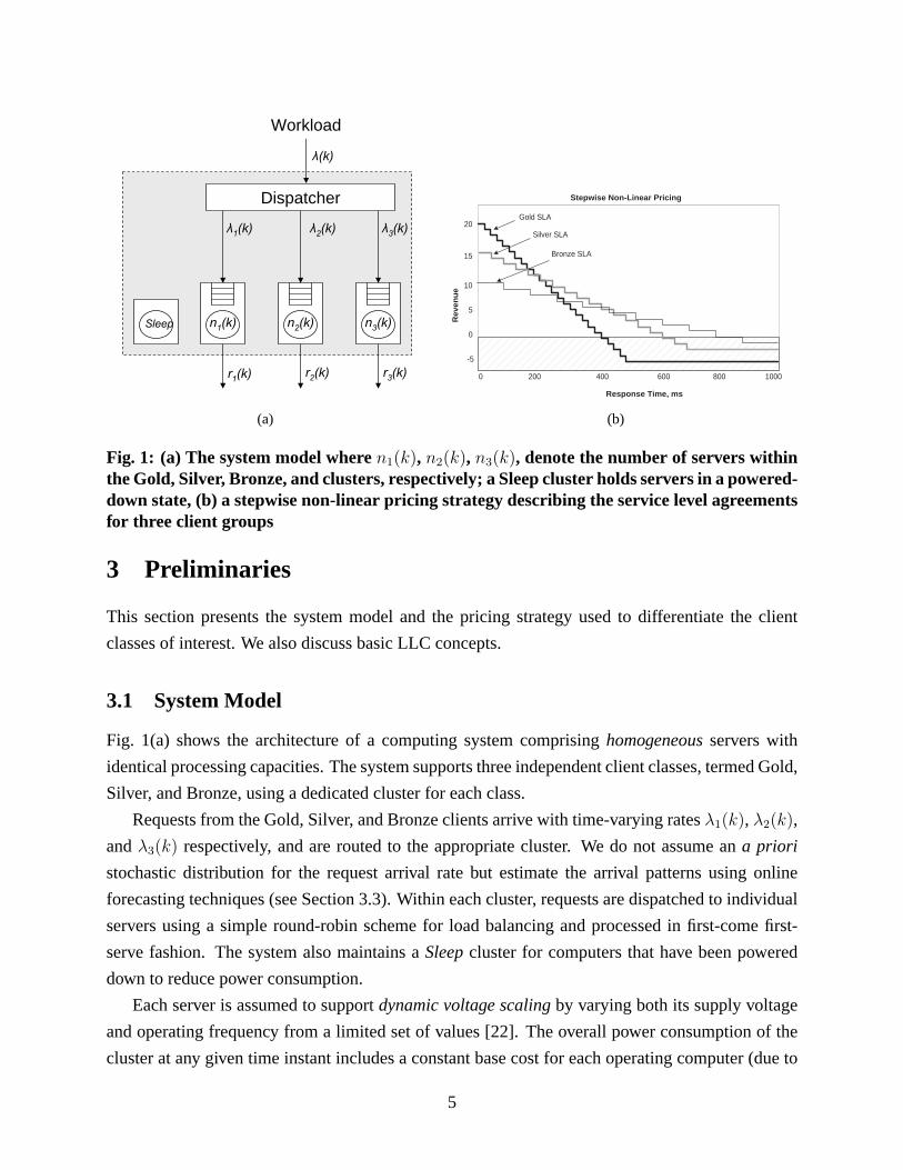
Fig. 1: (a) The system model wheren1(k), n2(k), n3(k), denote the number of servers withinthe Gold, Silver, Bronze, and clusters, respectively; a Sleep cluster holds servers in a powered-down state, (b) a stepwise non-linear pricing strategy describing the service level agreementsfor three client groups

3 Preliminaries

This section presents the system model and the pricing strategy used to differentiate the client

classes of interest. We also discuss basic LLC concepts.

3.1 System Model

Fig. 1(a) shows the architecture of a computing system comprisinghomogeneousservers with

identical processing capacities. The system supports three independent client classes, termed Gold,

Silver, and Bronze, using a dedicated cluster for each class.

Requests from the Gold, Silver, and Bronze clients arrive with time-varying ratesλ1(k), λ2(k),

andλ3(k) respectively, and are routed to the appropriate cluster. We do not assume ana priori

stochastic distribution for the request arrival rate but estimate the arrival patterns using online

forecasting techniques (see Section 3.3). Within each cluster, requests are dispatched to individual

servers using a simple round-robin scheme for load balancing and processed in first-come first-

serve fashion. The system also maintains aSleepcluster for computers that have been powered

down to reduce power consumption.

Each server is assumed to supportdynamic voltage scalingby varying both its supply voltage

and operating frequency from a limited set of values [22]. The overall power consumption of the

cluster at any given time instant includes a constant base cost for each operating computer (due to

5

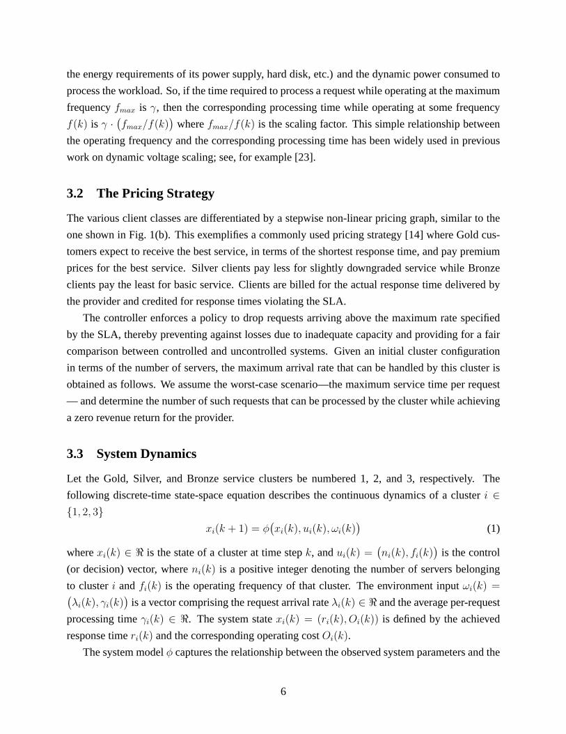
the energy requirements of its power supply, hard disk, etc.) and the dynamic power consumed to

process the workload. So, if the time required to process a request while operating at the maximum

frequencyfmax is γ, then the corresponding processing time while operating at some frequency

f(k) is γ ·(fmax/f(k)

)wherefmax/f(k) is the scaling factor. This simple relationship between

the operating frequency and the corresponding processing time has been widely used in previous

work on dynamic voltage scaling; see, for example [23].

3.2 The Pricing Strategy

The various client classes are differentiated by a stepwise non-linear pricing graph, similar to the

one shown in Fig. 1(b). This exemplifies a commonly used pricing strategy [14] where Gold cus-

tomers expect to receive the best service, in terms of the shortest response time, and pay premium

prices for the best service. Silver clients pay less for slightly downgraded service while Bronze

clients pay the least for basic service. Clients are billed for the actual response time delivered by

the provider and credited for response times violating the SLA.

The controller enforces a policy to drop requests arriving above the maximum rate specified

by the SLA, thereby preventing against losses due to inadequate capacity and providing for a fair

comparison between controlled and uncontrolled systems. Given an initial cluster configuration

in terms of the number of servers, the maximum arrival rate that can be handled by this cluster is

obtained as follows. We assume the worst-case scenario—the maximum service time per request

— and determine the number of such requests that can be processed by the cluster while achieving

a zero revenue return for the provider.

3.3 System Dynamics

Let the Gold, Silver, and Bronze service clusters be numbered 1, 2, and 3, respectively. The

following discrete-time state-space equation describes the continuous dynamics of a clusteri ∈{1, 2, 3}

xi(k + 1) = φ(xi(k), ui(k), ωi(k)

)(1)

wherexi(k) ∈ < is the state of a cluster at time stepk, andui(k) =(ni(k), fi(k)

)is the control

(or decision) vector, whereni(k) is a positive integer denoting the number of servers belonging

to clusteri andfi(k) is the operating frequency of that cluster. The environment inputωi(k) =(λi(k), γi(k)

)is a vector comprising the request arrival rateλi(k) ∈ < and the average per-request

processing timeγi(k) ∈ <. The system statexi(k) = (ri(k), Oi(k)) is defined by the achieved

response timeri(k) and the corresponding operating costOi(k).

The system modelφ captures the relationship between the observed system parameters and the

6

control inputs that adjust these parameters. We obtainφ from first principles using the following

difference queuing model.

qi(k + 1) =qi(k) +(λi(k)− pi(k)

)· ts (2)

pi(k) =ni(k)

γi(k)· fi(k)

fmax

(3)

ri(k + 1) =γi(k) +qi(k + 1)

pi(k)(4)

Oi(k) =ni(k) ·(c0 + c1 · fi(k)3

)(5)

The queue length at time step(k + 1) is given by the current queue lengthqi(k) and the ar-

rival and processing ratesλi(k) and pi(k), respectively. The processing ratepi(k) is given by

the cluster capacity, in terms of the number of serversni(k), and the average service timeγi(k).

The response time,ri(k + 1) is a sum of the average service timeγi(k) plus waiting time in the

queue(qi(k + 1)/pi(k)

). The operating costOi(k) of the cluster is obtained in terms of its overall

power consumption. Each server incurs a base (or idle) power consumption costc0 and a dynamic

cost dependent upon the cubic operating frequencyfi(k)3 multiplied by a scaling constantc1 as

described in [23]. Table 1 in Section 6 lists the specific parameters forc0 andc1.

The above equations adequately model the system dynamics of a cluster when the workload is

mostly CPU intensive, i.e., the processor on each server is the bottleneck resource. Typically, this

is true for web and e-commerce servers where both the application and data can be fully cached in

memory, thereby minimizing (or eliminating) costly hard disk accesses.

3.4 The Control Problem

The overall control objective is to maximize profit over all service classes while minimizing the

operating costs related to power consumption. Servers can be switched between different clusters

or new ones turned on. The system operating cost, in terms of its power consumption, must also

be reduced by deciding the frequency at which to operate the servers within each cluster and the

number of unused servers to power down. Generally speaking, this performance control problem

can be posed as a sequential optimization problem under uncertainty, i.e., the problem may need

continuous re-solving with observed environmental events such as time-varying client workload

patterns and server failures.

A practical solution to the resource provisioning problem in enterprise systems must also ad-

dress the following key issues.

• Hybrid system behavior. Computing systems exhibit hybrid behavior comprising both discrete-

event and time-based dynamics [24] and the control decisions that may be issued to the sys-

7

tem are typically limited to a finite set at any given time. For example, in Fig. 1(a), only a

limited number of servers can be moved between clusters, and each server can only choose

from a finite and discrete set of possible operating frequencies.

• Optimization under constraints. To maximize profit, our system must maximize the revenue

generated from the clients and minimize its operating cost. The corresponding (nonlinear)

cost function includes multiple control variables and must be optimized under dynamic con-

straints.

• Control actions with dead times. Actions such as powering up a server on demand in-

cur some dead time—the delay between a control decision and the corresponding system

response—requiringproactive controlwhere decisions must be provided in anticipation of

future changes in operating conditions.

• Cost of control. In a practical setting, certain control decisions themselves incur significant

cost. In our example, revenue is lost while a server is being switched between clients if

that server remains unavailable for some time duration while a different operating system

and/or application environment is loaded to service the new client. Other switching costs

may include the excess power consumed by a server when booting up or powering down.

• Risky control decisions. When the incoming workload is highly variable, each provisioning

decision made by the controller is risky. For example, switching servers excessively between

clusters may actually reduce profit generation, especially in the presence of the switching

costs described above.

• Real-time operation. Since workload intensity can change quite quickly in an enterprise sys-

tem [9, 25], control strategies must adapt to such variations and provision system resources

over short time scales, usually on the order of10s of seconds or a few minutes. These

strategies complement the more traditional offline capacity planning process [26].

The variables to be decided by the controller at each sampling intervalk are the number of servers

ni(k) and the overall operating frequencyfi(k) of these servers for clusteri ∈ {1, 2, 3}. Relevant

parametersλi(k) and γi(k) of the operating environment are estimated, and used by the system

model discussed in Section 3.3, to forecast future behavior over the specified prediction horizon,

h. Since the current values of the environment inputs cannot be measured until the next sampling

instant, the corresponding system state can only be estimated as follows:

xi(k + 1) = φ(xi(k), ui(k), ωi(k)

)(6)

8

Here,ωi(k) =(λi(k), γi(k)

), whereλi(k) andγi(k) denote the estimated request arrival rate

and processing time, respectively. We use an ARIMA model [27], implemented via a Kalman

filter [28], to estimateλi(k). The service time for requests is estimated using an exponentially-

weighted moving-average (EWMA) filter specified by the expressionγi(k + 1) = π · γi(k) + (1−π) · γi(k − 1) whereπ is a smoothing constant.

The LLC approach constructs a set of future states from the current statex(k) up to a prediction

horizonh. A trajectory{u∗i (j)|j ∈ [k+1, k+h]} of resource provisioning decisions for each cluster

i that maximizes the system utility while satisfying both state and input constraints is selected

within this horizon. The first input leading to this trajectory is chosen as the next control action.

The process is repeated at timek+1 when the new system statex(k+1) is available. The basic LLC

objective formulation shown in (7) accounts for future changes in the desired system trajectory and

measurable disturbances (e.g., environment inputs) and includes them as part of the overall control

design.

maxU

k+h∑j=k+1

J(x(j), u(j)

)(7)

Subject to: H(φ(x(j), u(j), ω(j))

)≤ 0

u(j) ∈ U(x(j))

Here,U denotes the set of all available control decisions andJ is the utility function to be

optimized (discussed next in Section 4). We express in a general form the set of constraints

upon the system state, control actions, and environmental inputs, respectively, with the inequal-

ity H(φ(x(j), u(j), ω(j))

)≤ 0.

In a computing system where control inputs must be chosen from discrete values, the optimiza-

tion problem in (7) will show an exponential increase in worst-case complexity with an increasing

number of control options and longer prediction horizons. In this paper, we substantially reduce

the dimensionality of the optimization problem using localized (or bounded) search techniques.

4 Problem Formulation

This section formulates the profit maximization problem under uncertain operating conditions.

When workload parameters are highly dynamic and variable, the corresponding forecast values

typically have errors or inaccuracies. Therefore, we address how our design tackles such forecast-

ing errors using two complementary techniques: (1) encoding the risk inherent to control decisions

into the problem formulation itself; and (2) including a discounting factor during lookahead opti-

mization to mitigate forecasting errors on control decisions.

9

4.1 The Profit Maximization Problem

The profitRi(xi(k), ni(k), fi(k)) generated by a computing clusteri at timek, given the current

statexi(k), cluster capacityni(k), and operating frequencyfi(k) is:

Ri

(xi(k), ni(k), fi(k)

)=

li(ri(k)

)−O

(ni(k), fi(k)

)− S

(∆ni(k)

)(8)

whereli(ri(k)) is the revenue generated by clusteri, as per the SLA function shown in Fig. 1(b),

for the achieved average response timeri(k) andO(ni(k), fi(k)

)denotes the operating cost. The

switching cost incurred by the cluster due to the provisioning decision is denoted byS(∆ni(k)).

This cost is a function of the number of servers moved between different client clusters, including

the Sleep cluster, and accounts for power consumption costs incurred while starting up computers,

plus the revenue lost when the computer is unavailable to perform any useful service for some

duration (e.g., a different operating system and/or application must be loaded to service the client).

The profit maximization problem for the three service classesi ∈ {1, 2, 3} is then posed as

follows:

Compute:

maxN,F

k+h∑j=k+1

3∑i=1

Ri

(xi(j), ni(j), fi(j)

)(9)

Subject to:

ni(j) ≥ Kmin ∀j

The formulation in ( 9) is solved over all possible options in the finite control setN (number

of servers) andF (set of operating frequencies) under explicit and dynamic constraints, reflecting

current operating conditions such as the number of available computers and the overall energy

budget for the system. Human operators may also enforce specific controller behavior using con-

straints. For example in ( 9), the controller is instructed to maintain a minimum cluster sizeKmin

at all times to accommodate sudden (and rare) bursts of high traffic caused by flash crowds [29],

thereby ensuring conservative performance.

4.2 Encoding Risk in the Cost Function

Many real workload traces, including those from the WC98 web site and others [25,30] show high

variability within short time periods, where characteristics such as request arrival rates change

quite significantly and quickly - usually on the order of a few minutes. Therefore, forecasts of such

10

environmental parameters typically incur errors or inaccuracies where the observed values differ

from the corresponding predictions.

When arrivals are noisy, the controller may constantly switch computers between clients in

an effort to maximize profit generation. However, due to switching costs, excessive switching is

risky and may actually reduce the profit generated. Therefore, in an uncertain operating environ-

ment where control decisions are risky, the optimization problem formulated in (9) may not be

the most appropriate way to measure a controller’s preference between different provisioning deci-

sions. Therefore, we explicitly encode risk in the problem formulation using preference functions

to order possible controller decisions. Using such functions to aid decision making under uncer-

tainty has been previously studied in the context of Investment Analysis [31] as well as dynamic

programming [32].

In noisy conditions, the estimated workload parameterλi(k) typically has an uncertainty band

±εi(k) around it, whereεi(k) = ‖λi(k) − λi(k)‖ denotes the (average) observed error between

the actual and forecasted values. Then, given a current statexi(k) and possible control inputs

ni(k) andfi(k), we can generate a set of estimated future states, each corresponding to someλi(k)

value in the uncertainty band. We can now augment the state-generation equation in (6) with the

following new expression that considers three possible arrival-rate estimates,λi(j) − εi(j), λi(j),

and,λi(j) + εi(j), for each stepj within the prediction horizonh to form a corresponding set of

possible future states.

Xi(j) ={f(xi(j − 1), ui(j), ([λi(j) + εi], γi(j)))

}(10)

εi ∈ {−εi(j), 0, εi(j)}

Given this collection of states obtained within the uncertainty bandλi(k) ± εi(k), we define

µ(Xi(j)) as the algebraic mean of the profit generated by the states∀ xi(j) ∈ Xi(j). We now

associate the followingquadratic preferenceor utility functionwith the setXi(j):

Ji(Xi(j)) = A · µ(Xi(j))− β ·(ν(Xi(j)) + µ(Xi(j))

2)

(11)

whereA > 2 · µ(Xi(j)) is a constant andβ is the risk preference factor. Here,µ(Xi(j)

)denotes

the mean profit generated by the states inXi(j) andν(Xi(j)

)denotes the variance among the dif-

ferent profit estimates. Equation (11) is a mean-variance model commonly used for stock portfolio

management under risky conditions [31]. The risk preference factor can be tuned to induce the de-

sired controller behavior among classifications of being risk averse (β > 0), risk neutral (β = 0),

or risk seeking (β < 0). Intuitively, a risk-averse controller, when given a choice between two

provisioning decisions generating nearly equal mean profit but with markedly different variance,

will prefer the decision with smaller variance.

11

In order for the utility function to produce sensible results, the coefficientβ must be chosen so

that the utility function maintains a concave downward shape when the response times violate the

SLA, revenue is lost and profits are less than zeroµ(Xi(j)

)< 0, and a convex upward shape when

the profits are greater than zeroµ(Xi(j)

)> 0. Choosing a sensible range forβ requires a priori

knowledge of the variance or setting a maximum allowable variance relative to the average profit.

If we let A = 3 · µ(Xi(j)

)and let the variance be proportional to mean profitµ

(Xi(j)

)such as

ν(Xi(j)

)= 0.5 · µ

(Xi(j)

), then differentiate the utility function with respect toµ

(Xi(j)

):

∂J

∂µ= 6 · µ

(Xi(j)

)− β

(0.5 + 2 · µ

(Xi(j)

))(12)

Solving Equation ( 12) for∂J∂µ

= 0 where the utility curve would change direction gives us:

∣∣β∣∣ <3 · µ

(Xi(j)

)0.25 + µ

(Xi(j)

) (13)

Equation ( 12) indicates that choosing a sensible range of possibleβ values requires having

some a priori knowledge about the expected variance within a given set of profit estimates. If

this is not possible due to the presence of noise within the workload, then a range forβ may be

computed by setting a maximum allowable variance as some scalar multiple of the mean profit

µ(Xi(j)

). Having defined our utility function in ( 11) and an expression for the range ofβ risk

preference values in ( 13), we now modify the profit maximization problem in (9) to one ofutility

maximization.

Compute:

maxN,F

k+h∑j=k+1

3∑i=1

J(Xi(j), ni(j), fi(j)

)(14)

Subject to:

ni(j) ≥ Kmin∀j

4.3 Adding a Discounting Factor

In an uncertain operating environment, we expect the workload and environmental parameter esti-

mations, and thus, the estimated system states to become increasingly inaccurate as we go deeper

into the prediction horizon, degrading control performance. One can mitigate the effects of fore-

casting inaccuracies on control performance by associating a discounting factor with the cost func-

tion. Returning to the formulation in (9), let us associate a factorαj such that0 < α < 1, with the

cost functionR. If α < 1, then future costs matter less than the same costs incurred at the present

time, i.e., states further out in the prediction horizon have less impact on the current control action.

12

Predictor Model )( jr Controller

)(),( jfjn

)(ˆ),(ˆ jj γλ

Workload

Predictor Model)(),( kk γλ )(ˆ jr Controller

)(),( jfjn

)(kqSystem

)(),( ** kfkn

(a)

x(k)

)1(ˆ +jx

)2(ˆ +jx

)3(ˆ +jx

)(ˆ hjx +

hkjk +≤< :horizon Prediction

(b)

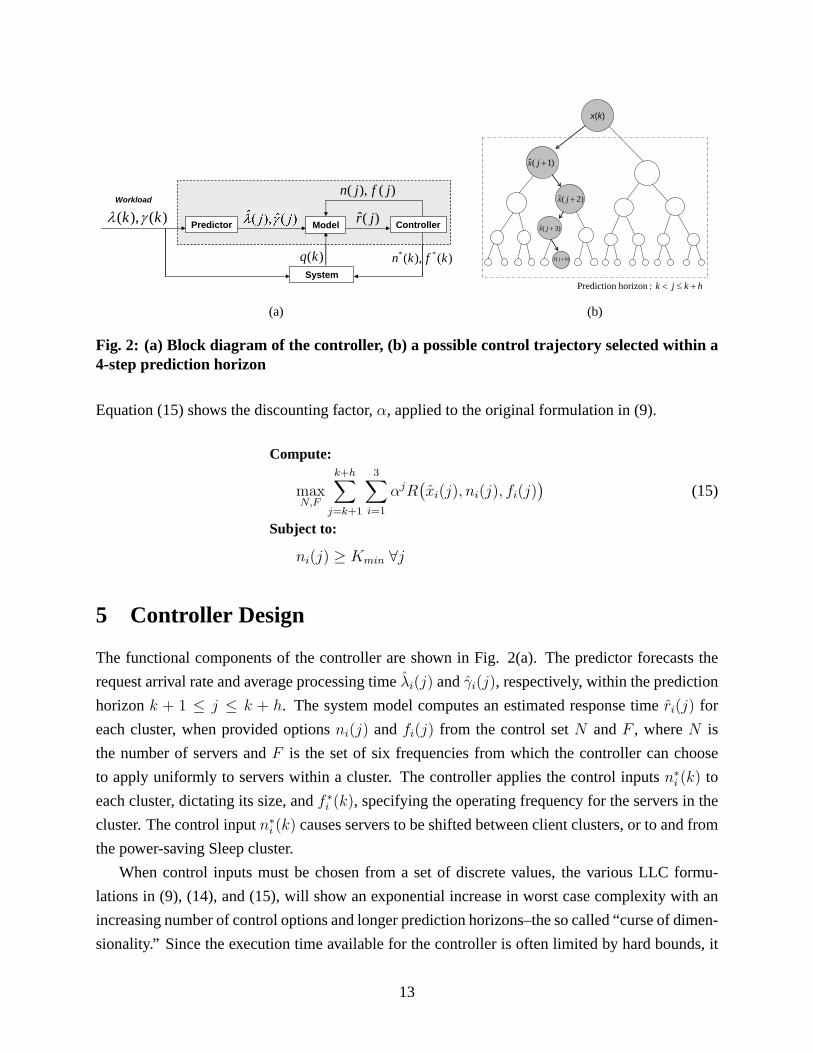
Fig. 2: (a) Block diagram of the controller, (b) a possible control trajectory selected within a4-step prediction horizon

Equation (15) shows the discounting factor,α, applied to the original formulation in (9).

Compute:

maxN,F

k+h∑j=k+1

3∑i=1

αjR(xi(j), ni(j), fi(j)

)(15)

Subject to:

ni(j) ≥ Kmin ∀j

5 Controller Design

The functional components of the controller are shown in Fig. 2(a). The predictor forecasts the

request arrival rate and average processing timeλi(j) andγi(j), respectively, within the prediction

horizonk + 1 ≤ j ≤ k + h. The system model computes an estimated response timeri(j) for

each cluster, when provided optionsni(j) andfi(j) from the control setN andF , whereN is

the number of servers andF is the set of six frequencies from which the controller can choose

to apply uniformly to servers within a cluster. The controller applies the control inputsn∗i (k) to

each cluster, dictating its size, andf ∗i (k), specifying the operating frequency for the servers in the

cluster. The control inputn∗i (k) causes servers to be shifted between client clusters, or to and from

the power-saving Sleep cluster.

When control inputs must be chosen from a set of discrete values, the various LLC formu-

lations in (9), (14), and (15), will show an exponential increase in worst case complexity with an

increasing number of control options and longer prediction horizons–the so called “curse of dimen-

sionality.” Since the execution time available for the controller is often limited by hard bounds, it

13

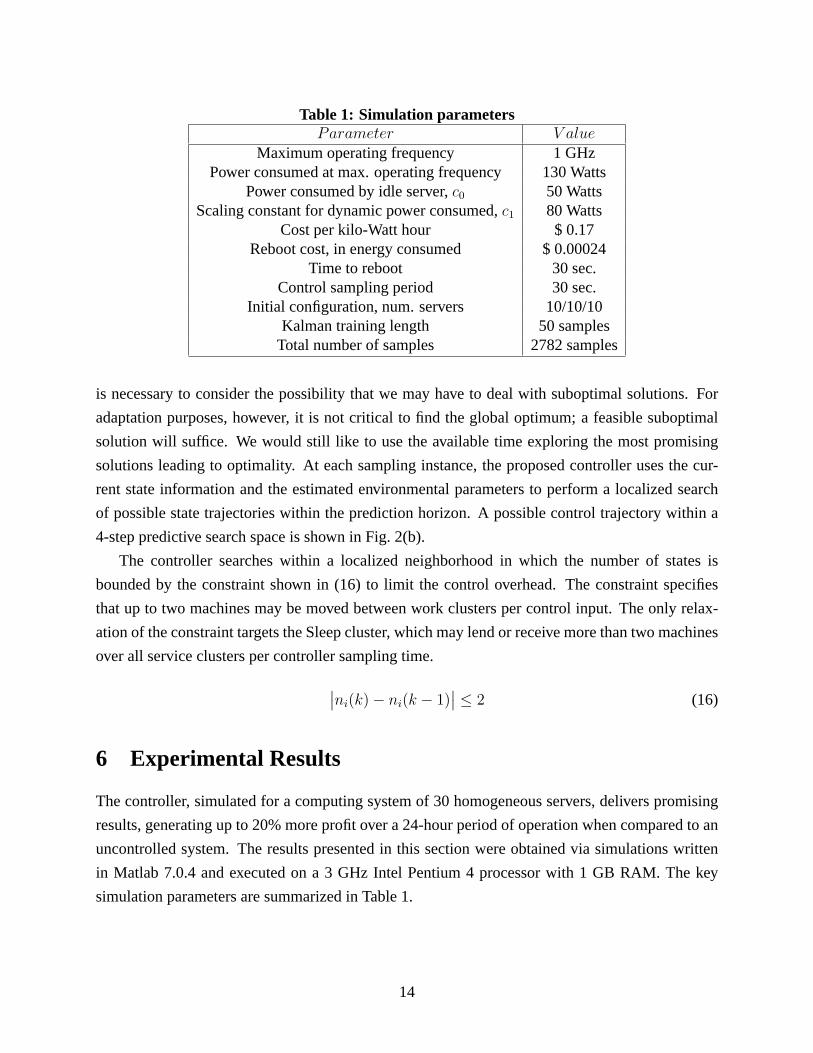
Table 1: Simulation parametersParameter V alue

Maximum operating frequency 1 GHzPower consumed at max. operating frequency 130 Watts

Power consumed by idle server,c0 50 WattsScaling constant for dynamic power consumed,c1 80 Watts

Cost per kilo-Watt hour $ 0.17Reboot cost, in energy consumed $ 0.00024

Time to reboot 30 sec.Control sampling period 30 sec.

Initial configuration, num. servers 10/10/10Kalman training length 50 samples

Total number of samples 2782 samples

is necessary to consider the possibility that we may have to deal with suboptimal solutions. For

adaptation purposes, however, it is not critical to find the global optimum; a feasible suboptimal

solution will suffice. We would still like to use the available time exploring the most promising

solutions leading to optimality. At each sampling instance, the proposed controller uses the cur-

rent state information and the estimated environmental parameters to perform a localized search

of possible state trajectories within the prediction horizon. A possible control trajectory within a

4-step predictive search space is shown in Fig. 2(b).

The controller searches within a localized neighborhood in which the number of states is

bounded by the constraint shown in (16) to limit the control overhead. The constraint specifies

that up to two machines may be moved between work clusters per control input. The only relax-

ation of the constraint targets the Sleep cluster, which may lend or receive more than two machines

over all service clusters per controller sampling time.

∣∣ni(k)− ni(k − 1)∣∣ ≤ 2 (16)

6 Experimental Results

The controller, simulated for a computing system of 30 homogeneous servers, delivers promising

results, generating up to 20% more profit over a 24-hour period of operation when compared to an

uncontrolled system. The results presented in this section were obtained via simulations written

in Matlab 7.0.4 and executed on a 3 GHz Intel Pentium 4 processor with 1 GB RAM. The key

simulation parameters are summarized in Table 1.

14

��������������

0

1e-5Gold SLA

Silver SLA

Bronze SLA

Response Time, ms

Rev

enu

e, d

olla

rs

7e-6

3e-6

-3e -6

0 200 400 600

Stepwise Non-Linear Pricing of Service Level Agreements

(a)

0 500 1000 1500 2000 25000

200

400

600

800

1000

1200

1400

Time Instance

Arr

ival

Rat

e P

er 3

0 S

econ

d In

terv

al

1998 World Cup HTTP Requests − Original Workload

Gold Workload

Silver Workload

Bronze Workload

(b)

0 500 1000 1500 2000 25000

100

200

300

400

500

600

700

Time Instance

Arr

ival

Rat

e P

er 3

0 S

econ

d In

terv

al

Kalman Filter Estimate for Gold Workload − Original Workload

Kalman Estimate t+1, dotted line

Gold Workload, solid line

(c)

0 500 1000 1500 2000 25000

200

400

600

800

1000

1200

1400

Arr

ival

Rat

e P

er 3

0 S

econ

d In

terv

al

Time Instance

1998 World Cup HTTP Requests − Noisy Workload

Silver Workload

Gold Workload

Bronze Workload

(d)

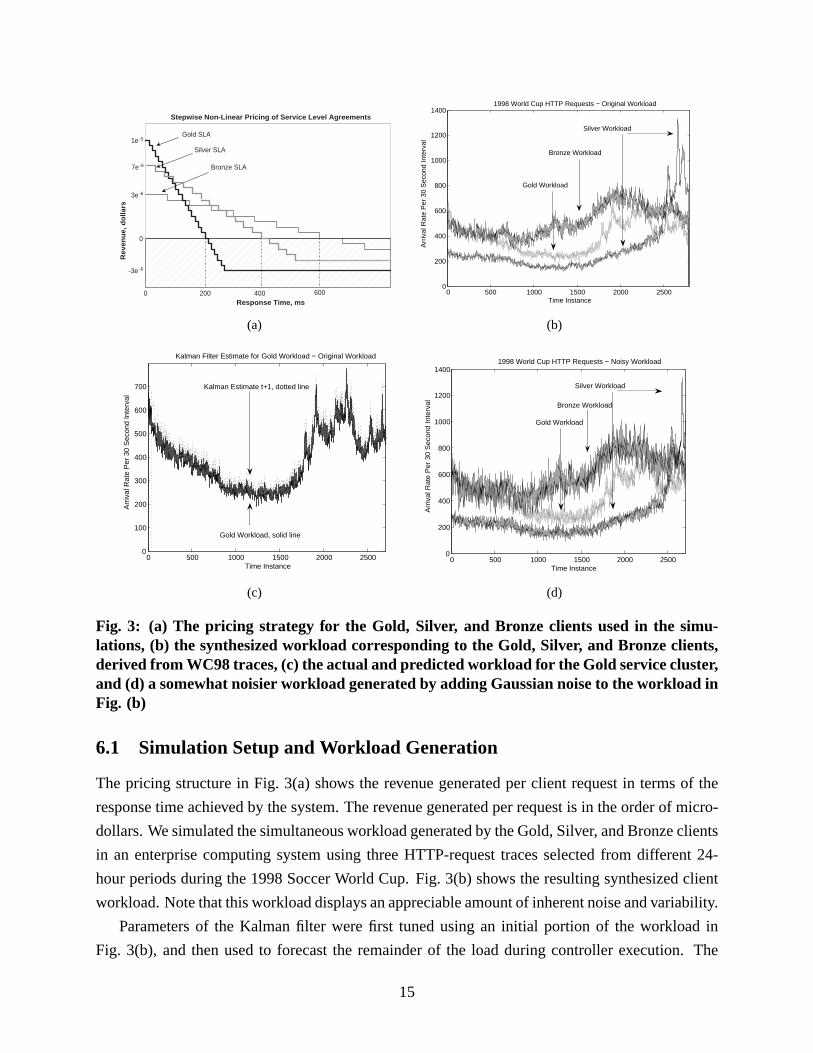
Fig. 3: (a) The pricing strategy for the Gold, Silver, and Bronze clients used in the simu-lations, (b) the synthesized workload corresponding to the Gold, Silver, and Bronze clients,derived from WC98 traces, (c) the actual and predicted workload for the Gold service cluster,and (d) a somewhat noisier workload generated by adding Gaussian noise to the workload inFig. (b)

6.1 Simulation Setup and Workload Generation

The pricing structure in Fig. 3(a) shows the revenue generated per client request in terms of the

response time achieved by the system. The revenue generated per request is in the order of micro-

dollars. We simulated the simultaneous workload generated by the Gold, Silver, and Bronze clients

in an enterprise computing system using three HTTP-request traces selected from different 24-

hour periods during the 1998 Soccer World Cup. Fig. 3(b) shows the resulting synthesized client

workload. Note that this workload displays an appreciable amount of inherent noise and variability.

Parameters of the Kalman filter were first tuned using an initial portion of the workload in

Fig. 3(b), and then used to forecast the remainder of the load during controller execution. The

15

Kalman filter produces good estimates of the arrival rate with a small amount of error, as illustrated

for the Gold cluster in Fig. 3(c). As shown in Fig. 3(d), we also generated a somewhat noisier

workload by adding random Gaussian noise to the original workload in Fig. 3(b). The Kalman

filter produces estimates within an average of 6% error from the actual values of this workload.

To generate the processing times for individual requests within the arrival sequence in Fig. 3(d),

we assumed processing times within a range that reflects a mix of static and dynamic page re-

quests [33]. We generated a virtual store comprising 10,000 objects, and the time needed to

process an object request was randomly chosen from a uniform distribution between [1.0, 43.0]

ms. The distribution of individual requests within the arrival sequence was determined using two

key characteristics of most web workloads:

• Popularity: It has been observed that a few files are extremely popular while many others

are rarely requested, and that the popularity distribution commonly follows Zipf’s law [34].

Therefore, we partitioned the virtual store in two—a “popular” set with 1000 objects re-

ceiving 90% of all requests, and a “rare” set containing the remaining objects in the store

receiving only 10% of requests.

• Temporal locality: This is the likelihood that once an object is requested, it will be requested

again in the near future. In many web workloads, temporal locality follows a lognormal

distribution [35].

The static cluster size for an uncontrolled computing system or the initial configuration for a con-

trolled one is determined using the maximum arrival rate observed within the workload of interest

(Fig. 3(d)), and the maximum service time of a dynamic page, set at 43 ms [33]. Given this arrival

rate and processing time, the initial configuration for each cluster is simply the number of servers

needed to achieve the response time corresponding to a revenue generation of zero dollars (the

break-even point in Fig. 3(a)).

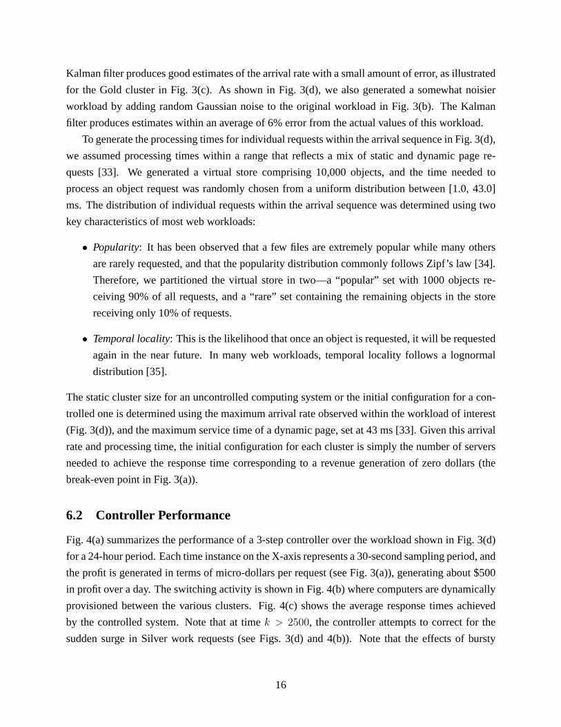
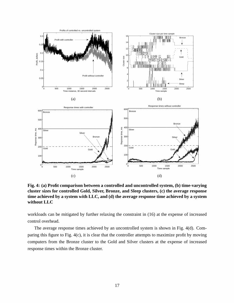
6.2 Controller Performance

Fig. 4(a) summarizes the performance of a 3-step controller over the workload shown in Fig. 3(d)

for a 24-hour period. Each time instance on the X-axis represents a 30-second sampling period, and

the profit is generated in terms of micro-dollars per request (see Fig. 3(a)), generating about $500

in profit over a day. The switching activity is shown in Fig. 4(b) where computers are dynamically

provisioned between the various clusters. Fig. 4(c) shows the average response times achieved

by the controlled system. Note that at timek > 2500, the controller attempts to correct for the

sudden surge in Silver work requests (see Figs. 3(d) and 4(b)). Note that the effects of bursty

16

0 500 1000 1500 2000 25000

0.05

0.1

0.15

0.2

0.25

0.3

Time instance, 30 second intervals

Pro

fit, d

olla

rs

Profits of controlled vs. uncontrolled system

Profit without controller

Profit with controller

(a)

0 500 1000 1500 2000 25000

2

4

6

8

10

12

14

16

Time sample

Clu

ster

siz

e

Cluster size per time sample

Gold

Sleep

Silver

Bronze

(b)

0 500 1000 1500 2000 25000

100

200

300

400

500

600

Time sample

Rep

onse

tim

e, m

s

Response times with controller

Gold

Silver

Bronze

Bronze

Silver

Gold

(c)

0 500 1000 1500 2000 25000

100

200

300

400

500

600

Time sample

Rep

onse

tim

e, m

s

Response times without controller

Gold

Silver

Bronze

Bronze

Silver

Gold

(d)

Fig. 4: (a) Profit comparison between a controlled and uncontrolled system, (b) time-varyingcluster sizes for controlled Gold, Silver, Bronze, and Sleep clusters, (c) the average responsetime achieved by a system with LLC, and (d) the average response time achieved by a systemwithout LLC

workloads can be mitigated by further relaxing the constraint in (16) at the expense of increased

control overhead.

The average response times achieved by an uncontrolled system is shown in Fig. 4(d). Com-

paring this figure to Fig. 4(c), it is clear that the controller attempts to maximize profit by moving

computers from the Bronze cluster to the Gold and Silver clusters at the expense of increased

response times within the Bronze cluster.

17

6.3 Effects of Parameter Tuning

We now compare the profit earned by various configurations of the online controller. Again, our

base case is a computing system without online control. We have assumed an average request

processing time of 23 ms for each of the three client classes. We show experimental results for the

following controller types:

• A controller that only moves servers between clusters without impacting the operating fre-

quency, i.e., servers operate at one frequencyfmax. Both 2- and 3-step prediction horizons

are considered.

• A controller that moves servers between clusters while simultaneously deciding the operat-

ing frequency of each cluster. Again, both 2- and 3-step prediction horizons are considered.

Table 1 shows the base controller parameters used within our simulations. We test the controller in

operating environments with and without the addition of noise, i.e., using both Figs. 3(b) and 3(d).

Our simulations indicate that the above controllers achieve at least 10% in profit gains and in some

cases slightly more than 20% in profit gains.

Our simulations also sought to quantify the effects of incorporating operating frequency into

the control set. The controller may now choose from a set of six operating frequencies. Assuming

a maximum frequencyfmax = 1GHz for each server, the various operating frequencies were

obtained as{0.5 ·fmax, 0.6 ·fmax, ..., 1.0 ·fmax}. Adding operating frequencies to the control set has

the following advantages when provisioning computing resources. First, frequency scaling can be

done almost instantaneously with little transient switching cost. Second, changing the operating

frequency allows a cluster to control costs via a cubic relationship between operating frequency and

power consumption [23] while still retaining the resource in an active state to handle unpredicted

bursts in the workload. In fact, Figs. 5(a) and-6(a) show that a controller that provisions both

the cluster size and operating frequency achieves 2-5% more in profit gains than a controller that

provisions only for cluster size.

First, we explore the effect of varyingβ, the risk preference factor previously introduced in

(11), on profit generation. Given the workload in Figs. 3(b) and 3(d), the corresponding perfor-

mance plots in Figs. 5(a) and 5(b) show that a risk-averse controllerβ > 0 performs better than

a risk-seeking oneβ < 0, an effect that is somewhat more pronounced when the workload has

increased variability. We also see that the performance of the controller drops off for largerβ val-

ues, both positive and negative. Large negative values forβ cause the controller to take more risks

during resource provisioning, thereby constantly moving servers between the various clusters and

reacting quickly to variations in the incoming workload. As noted in Section 1, this constant move-

ment of computing resources between clusters can result in lost profit in the presence of switching

18

−10 −8 −6 −4 −2 0 2 4 6 8 102

4

6

8

10

12

14

16

18

20

22

Beta value

Pro

fit g

ain,

per

cent

Profit Gain (%) for Beta ValuesOriginal Workload

2−step3−step2−step, frequency set3−step, frequency set

(a)

−10 −8 −6 −4 −2 0 2 4 6 8 102

4

6

8

10

12

14

16

18

20

22

Beta value

Pro

fit g

ain,

per

cent

Profit Gain (%) for Beta ValuesNoise Added to Workload

2−step3−step2−step, frequency set3−step, frequency set

(b)

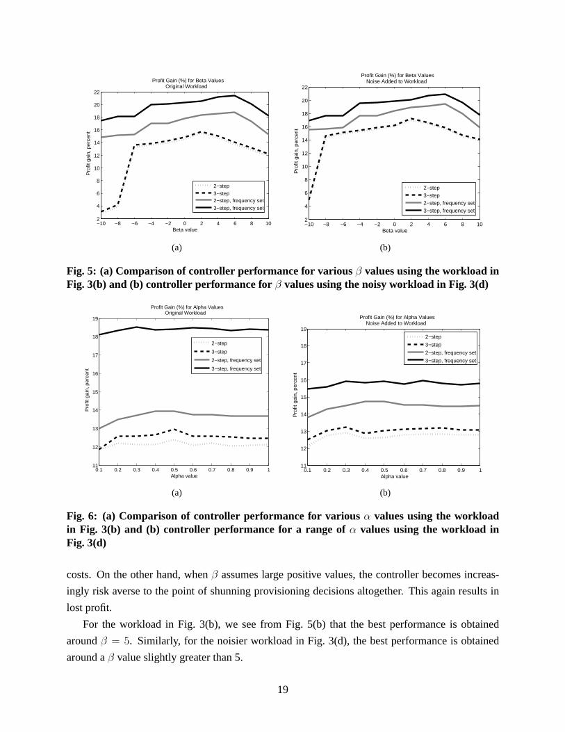
Fig. 5: (a) Comparison of controller performance for variousβ values using the workload inFig. 3(b) and (b) controller performance for β values using the noisy workload in Fig. 3(d)

0.1 0.2 0.3 0.4 0.5 0.6 0.7 0.8 0.9 111

12

13

14

15

16

17

18

19

Alpha value

Pro

fit g

ain,

per

cent

Profit Gain (%) for Alpha ValuesOriginal Workload

2−step

3−step

2−step, frequency set

3−step, frequency set

(a)

0.1 0.2 0.3 0.4 0.5 0.6 0.7 0.8 0.9 111

12

13

14

15

16

17

18

19

Alpha value

Pro

fit g

ain,

per

cent

Profit Gain (%) for Alpha ValuesNoise Added to Workload

2−step

3−step

2−step, frequency set

3−step, frequency set

(b)

Fig. 6: (a) Comparison of controller performance for various α values using the workloadin Fig. 3(b) and (b) controller performance for a range of α values using the workload inFig. 3(d)

costs. On the other hand, whenβ assumes large positive values, the controller becomes increas-

ingly risk averse to the point of shunning provisioning decisions altogether. This again results in

lost profit.

For the workload in Fig. 3(b), we see from Fig. 5(b) that the best performance is obtained

aroundβ = 5. Similarly, for the noisier workload in Fig. 3(d), the best performance is obtained

around aβ value slightly greater than 5.

19

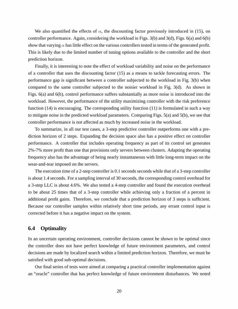
We also quantified the effects ofα, the discounting factor previously introduced in (15), on

controller performance. Again, considering the workload in Figs. 3(b) and 3(d), Figs. 6(a) and 6(b)

show that varyingα has little effect on the various controllers tested in terms of the generated profit.

This is likely due to the limited number of tuning options available to the controller and the short

prediction horizon.

Finally, it is interesting to note the effect of workload variability and noise on the performance

of a controller that uses the discounting factor (15) as a means to tackle forecasting errors. The

performance gap is significant between a controller subjected to the workload in Fig. 3(b) when

compared to the same controller subjected to the noisier workload in Fig. 3(d). As shown in

Figs. 6(a) and 6(b), control performance suffers substantially as more noise is introduced into the

workload. However, the performance of the utility maximizing controller with the risk preference

function (14) is encouraging. The corresponding utility function (11) is formulated in such a way

to mitigate noise in the predicted workload parameters. Comparing Figs. 5(a) and 5(b), we see that

controller performance is not affected as much by increased noise in the workload.

To summarize, in all our test cases, a 3-step predictive controller outperforms one with a pre-

diction horizon of 2 steps. Expanding the decision space also has a positive effect on controller

performance. A controller that includes operating frequency as part of its control set generates

2%-7% more profit than one that provisions only servers between clusters. Adapting the operating

frequency also has the advantage of being nearly instantaneous with little long-term impact on the

wear-and-tear imposed on the servers.

The execution time of a 2-step controller is 0.1 seconds seconds while that of a 3-step controller

is about 1.4 seconds. For a sampling interval of 30 seconds, the corresponding control overhead for

a 3-step LLC is about 4.6%. We also tested a 4-step controller and found the execution overhead

to be about 25 times that of a 3-step controller while achieving only a fraction of a percent in

additional profit gains. Therefore, we conclude that a prediction horizon of 3 steps is sufficient.

Because our controller samples within relatively short time periods, any errant control input is

corrected before it has a negative impact on the system.

6.4 Optimality

In an uncertain operating environment, controller decisions cannot be shown to be optimal since

the controller does not have perfect knowledge of future environment parameters, and control

decisions are made by localized search within a limited prediction horizon. Therefore, we must be

satisfied with good sub-optimal decisions.

Our final series of tests were aimed at comparing a practical controller implementation against

an “oracle” controller that has perfect knowledge of future environment disturbances. We noted

20

that even if workload predictions are completely error free, the profit generated is only slightly

higher than the practical case where only imperfect predictions can be obtained. We selected the

best performing controller after extensive tuning—a 3-step frequency-selecting controller having

a risk-averse behavior defined byβ = 5—and found that having perfect workload predictions

increased profit gains by only 1%, from a 20.5% gain with prediction errors to 21.3% with no

errors. Again, the baseline case was an uncontrolled system.

7 Conclusions

We have presented an optimization framework to enable self-managing behavior in an enterprise

computing system serving multiple client classes. The proposed lookahead control algorithm aims

to maximize profit generation by dynamically provisioning computing resources between multi-

ple client clusters. The problem formulation includes switching costs and explicitly encodes the

risk associated with making provisioning decisions in an uncertain operating environment. Exper-

iments using the WC98 workload indicate that, over the operating period of one day, our controller

generates 10% to 20% more profit when compared to a computing system without dynamic con-

trol, and with a very low cost of control. A risk-averse controller achieved higher profit gains than

a risk-seeking one, and a 3-step lookahead controller capable of tuning both the cluster capacity

and operating frequency performed the best over all the controllers that were tested.

References

[1] A. Sahai, S. Singhal, V. Machiraju, and R. Joshi, “Automated policy-based resource construc-tion in utility computing environments,” inProc. of IEEE Symposium on Network Operationsand Management. IEEE, Apr. 2004, pp. 381–393.

[2] R. Murch,Autonomic Computing. Prentice-Hall, 2004.

[3] I. Corporation, “An architectural blueprint for autonomic computing,” Thomas J. WatsonResearch Center, Tech. Rep., Oct. 2004.

[4] J. Hellerstein, Y. Diao, S. Parekh, and D. Tilbury,Feedback Control of Computing Systems.Wiley-Interscience, 2004.

[5] S. Abdelwahed, N. Kandasamy, and S. Neema, “Online control for self-management in com-puting systems,” inProc. of Real-Time and Embedded Technology and Applications Sympo-sium (RTAS). IEEE, May 2004, pp. 368–375.

[6] A. Bryson,Applied Optimal Control: Optimization, Estimation, and Control. HemispherePublishing, 1984.

21

[7] N. Kandasamy, S. Abdelwahed, and J. Hayes, “Self-optimization in computer systems via on-line control: Application to power management,” inProc. of IEEE Intl. Conf. on AutonomicComputing (ICAC). IEEE, May 2004, pp. 54–61.

[8] J. Maciejowski,Predictive Control with Constraints. Prentice Hall, 2002.

[9] M. Arlitt and T. Jin, “Workload characterization of the 1998 world cup web site,” Hewlett-Packard Labs, Tech. Rep., Sept. 1999.

[10] Y. Chen, A. Das, W. Qin, A. Sivasubramaniam, Q. Wang, and N. Gautam, “Managing serverenergy and operational costs in hosting centers,” inProc. of ACM SIGMETRICS. ACM,June 2004, pp. 303–314.

[11] B. Urgaonkar, P. Shenoy, A. Chandra, and P. Goyal, “Dynamic provisioning of multi-tierinternet applications,” inProc. of IEEE Intl. Conf. on Autonomic Computing (ICAC). IEEE,June 2005, pp. 217–228.

[12] M. Bennani and D. Menasce, “Resource allocation for autonomic data centers using analyticperformance models,” inProc. of IEEE Intl. Conf. on Autonomic Computing (ICAC). IEEE,June 2005, pp. 229–240.

[13] G. Pacifici, M. Spreitzer, A. Tantawi, and A. Youssef, “Performance management for clusterbased web services,” IBM Research Labs, Tech. Rep., May 2003.

[14] J. Zhang, T. Hamalainen, and J. Joutsensalo, “Optimal resource allocation scheme for maxi-mizing revenue in the future ip networks,” inProc. of the 10th Asia-Pacific Conf. on Comm.and 5th Intl. Sym. on Multi-Dimensional Mobile Comm.IEEE, Sept 2004, pp. 128–132.

[15] K. K. J.L. Hellerstein and M. Surendra, “A framework for applying inventory control tocapacity management for utility computing,” Thomas J. Watson Research Center, Tech. Rep.,Oct. 2004.

[16] T. Osogami, M. Harchol-Balter, and A. Scheller-Wolf, “Analysis of cycle stealing withswitching cost,” inProc. of ACM SIGMETRICS. ACM, June 2003, pp. 184–195.

[17] D. Eager, E. Lazowska, and J. Zahorjan, “Adaptive load sharing in homogeneous distributedsystems,”IEEE Trans. on Software Engineering, vol. 12, no. 5, pp. 662–675, May 1986.

[18] A. Tantawi and D. Towsley, “Optimal static load balancing in distributed computer systems,”J. of the ACM, vol. 32, no. 2, pp. 445–65, May 1986.

[19] T. Mudge, “Power: A first-class architectural design constraint,”IEEE Computer, pp. 52–58,Apr. 2001.

[20] V. Sharma, A. Thomas, T. Abdelzaher, and K. Skadron, “Power-aware qos management inweb servers,” inProc. of IEEE Intl. Real-Time Systems Sym.IEEE, 2002, pp. 63–72.

[21] R. Mishra, N. Rastogi, Z. Dakai, D. Mosse, and R. Melhem, “Energy-aware scheduling fordistributed real-time systems,” inProc. of IEEE Parallel and Distributed Processing Sym.(IPDPS). IEEE, Apr. 2003, pp. 63–72.

22

[22] Enhanced Intel SpeedStep Tecnology for the Intel Pentium M Processor, Intel Corp., 2004.

[23] M. Elnozahy, M. Kistler, and R. Rajamony, “Energy-efficient server clusters,” inProc. of the2nd Workshop on Power-Aware Computing Systems (held with HPCA). HPCA, Feb. 2002,pp. 126–37.

[24] P. Antsaklis and A. Nerode, Eds.,Special Issue on Hybrid Control Systems, ser. IEEE Trans.Autom. Control, vol. 43, Apr. 1998.

[25] M. F. Arlitt and C. L. Williamson, “Web server workload characterization: The search forinvariants,” inProc. ACM SIGMETRICS Conf., 1996, pp. 126–137.

[26] D. Menasce and V. A. F. Almeida,Capacity Planning for Web Services: Metrics, Models,and Methods. Upper Saddle River, NJ: Prentice Hall PTR, 2002.

[27] G. Box, G. Jenkins, and G. Reinsel,Time Series Analysis: Forecasting and Control. PrenticeHall: Upper Saddle River, NJ, 1999.

[28] K. Brammer and G. Siffling,Kalman-Bucy Filters. Artec House: Norwood, MA, 1989.

[29] R. Morris and D. Lin, “Variance of aggregated web traffic,” inProc. of IEEE INFOCOM.IEEE, May 2000, pp. 360–366.

[30] J. Judge, “A model for the marginal distribution of aggregate per second http request rate,” inIEEE Wrkshp. on Local and Metropolitan Area Networks. IEEE, Nov. 1999, pp. 29–36.

[31] T. Copeland and J. Weston,Financial Theory and Corporate Policy, 3rd, ed.Addison-Wesley, 1988.

[32] Y. Bar-Shalom, “Stochastic dynamic programming: Caution and probing,”IEEE Trans. onAutomatic Control, vol. 26, no. 5, pp. 1184–1195, Oct. 1981.

[33] C. Rusu, A. Ferreira, C. Scordino, A. Watson, R. Melhem, and D. Mosse, “Energy-efficientreal-time heterogeneous server clusters,” inProc. of IEEE RTAS. IEEE, April 2006.

[34] M. Arlitt and C. Williamson, “Web server workload characterization: The search for invari-ants,” inProc. of ACM SIGMETRICS. ACM, 1996, pp. 126–37.

[35] P. Barford and M. Crovella, “Generating representative web workloads for network and serverperformance evaluation,” inProc. ACM SIGMETRICS Conf., 1998, pp. 151–160.

23