Embed Size (px)
Citation preview
River Bathymetry ToolkitRiver Bathymetry ToolkitRiver Bathymetry Toolkit
Air, Water, and Aquatic Environments ProgramAir, Water, and Aquatic Environments ProgramRocky Mountain Research StationRocky Mountain Research Station
ESSA Technologies, Ltd.ESSA Technologies, Ltd.
WorkbookWorkbook
A GIS Toolkit for Mapping the A GIS Toolkit for Mapping the InIn‐‐stream Environmentstream Environment
U.S. Forest Service322 E. Front St., Suite 401Boise, ID 83702 Suite 300, 1765 West 8th Avenue,
Vancouver BC Canada V6J 5C6
Table of Contents Disclaimer of Liability.................................................................................................................... 1
Citation............................................................................................................................................ 1
1. Introduction............................................................................................................................ 2
2. Downloading and Installation ................................................................................................ 3
3. General Work Flow Diagram................................................................................................. 3
4. Tutorial Tasks ........................................................................................................................ 7
RBT Basics ............................................................................................................................ 7
Task 1 – Getting Started ............................................................................................... 7
Task 2 – Create a Detrended Base Map and use the Detrend Tool .............................. 9
Task 3 – Use the Bankfull Tool to create a bankfull polygon .................................... 12
Task 4 – Establish the channel centerline with Thiessen Polygons............................ 15
Working with Cross Sections............................................................................................... 16
Task 5 – Creating and Importing Cross Sections........................................................ 16
Task 6 – Cross Section Explorer................................................................................. 20
Task 7 – Elevation Interpolation................................................................................. 24
Hydraulic geometry metrics................................................................................................. 25
Long Profile Metrics ............................................................................................................ 29
Task 8 – Calculating and Viewing River Kilometers ................................................. 29
Task 9 – Calculating Gradient and Sinuosity ............................................................. 32
Longitudinal Explorer.......................................................................................................... 35
Task 10 – Viewing riverbed attributes........................................................................ 35
Task 11 – Export to HEC-RAS................................................................................... 37
Task 12 – RBT Options .............................................................................................. 38
5. Glossary of Terms................................................................................................................ 40
6. References............................................................................................................................ 41

Disclaimer of Liability Neither the United States Government nor any of its employees makes any warranty, express or implied, for any purposes regarding the River Bathymetry Toolkit (RBT). This includes warranties of merchantability and fitness for any particular purpose. Furthermore, neither the United States Government nor any of its employees assumes any legal liability or responsibility for the accuracy, completeness, or usefulness of any information or products derived from the River Bathymetry Toolkit.
Citation To cite the River Bathymetry Toolkit in publications, use:
McKean, J., Nagel, D., Tonina, D., Bailey, P., Wright, C.W., Bohn, C., Nayegandhi, A., 2009. Remote sensing of channels and riparian zones with a narrow-beam aquatic-terrestrial lidar. Remote Sensing, 1, 1065-1096; doi:10.3390/rs1041065.
1

1. Introduction The River Bathymetry Toolkit (RBT) is a suite of algorithms that automatically interrogate high-resolution Digital Elevation Models (DEMs) of stream channels and floodplains and extract standard hydraulic geometry parameters at user-defined locations in the digital data. The RBT computes a variety of measures of channel cross-section geometry. The tools also georeference the cross section data to locations along a stream centerline, which allows rapid mapping of changes in channel geometry along the length of a stream. There are tools to compute gradient and sinuosity of streams over user-defined channel lengths. Finally, the RBT formats channel data for direct import to the 1D hydrodynamic flow model HEC-RAS [1]. While originally conceived by the US Forest Service to interpret data from the USGS aquatic-terrestrial Experimental Advanced Airborne Research Lidar (EAARL), the RBT will operate on any high-resolution DEM. It is very important to have a good quality DEM as data errors will often lead to issues with the RBT. To properly represent a channel in a digital format and extract reasonable hydraulic geometry values using the RBT, the source data must support a DEM that will have greater than about 5 pixels across the width of a channel. With a coarser DEM grid and fewer than about 5 pixels, the resolution of metrics, such as bankfull width, is poor. Channel geometry measurements in a DEM will always have lower precision and accuracy than achieved in traditional field-surveyed cross sections. However, the toolkit allows the user to construct far greater numbers of digital cross sections and to do so over much longer channel extents, limited only by the data coverage. The large numbers of digital channel cross sections that can be computed with the RBT also support much stronger statistical analyses of stream characteristics. Anyone is free to download the RBT and use it, subject to the disclaimer of liability by the US Forest Service and ESSA. We hope you find it useful. If you have questions about how to do something in the current RBT, your first contact should be Carolyn Bohn ([email protected]; 208 373 4367). If the RBT contributes in a significant way to your research, we would appreciate a citation (please cite as: McKean, J., Nagel, D., Tonina, D., Bailey, P., Wright, C.W., Bohn, C., Nayegandhi, A., 2009. Remote sensing of channels and riparian zones with a narrow-beam aquatic-terrestrial lidar. Remote Sensing, 1, 1065-1096; doi:10.3390/rs1041065). We view the current RBT as simply the first generation of an evolving toolkit. We encourage everyone to contribute to further development and expansion of the capabilities of the RBT, in the spirit of community-ware. You can do this by sending suggestions for improvements to Jim McKean ([email protected]) or Dave Nagel ([email protected]). We will evaluate your ideas and establish priorities for improvements in future versions. We also encourage you to develop your own GIS-based stream tools and contribute them to the RBT. Send your stream and floodplain GIS interpretation tools to Jim or Dave and we will test your algorithms and then incorporate them into the RBT. To support future development of the toolkit, we will have to generate money to fund our close collaborators, ESSA Technologies, Ltd. One way you can help is to send a note to Jim McKean, briefly describing your use of the RBT. We will then leverage those examples in future funding requests. (Alternatively, you could just send us money directly and expedite the whole process!).
2
In the near future a revolutionary change seems likely in how we map stream channels and stream networks, using technologies such as bathymetric lidars, boat-mounted acoustic sensors or optical remote sensing methods. Our vision for the RBT is a community-built and shared toolkit that quickly extracts the maximum information from these high-resolution digital data. How you use the RBT information – well that’s the science part of the story, and we hope you’ll accomplish many interesting and useful things. The main web page for the RBT, including sample data and documentation is at: http://www.fs.fed.us/rm/boise/AWAE/projects/river_bathymetry_toolkit.shtml. If you are interested in how we have used the EAARL and RBT, a summary of 6 years of research at the Forest Service, Boise Lab, is available from McKean et al. (2009) [2], at http://www.fs.fed.us/rm/pubs_other/rmrs_2009_mckean_j003.pdf.
2. Downloading and Installation The toolkit is implemented as a free extension to the desktop ArcGIS software from ESRI [3]. The toolkit may be downloaded from this website: http://www.essa.com/tools/RBT/download.html. The following are the System Requirements to install and run the toolkit.
• Microsoft Windows XP, Vista or 7. • Microsoft .Net Framework Version 2 Service Pack 1 ( Install Before installing
ArcGIS) • ESRI ArGIS Desktop 9.2 or newer. • Certain features of the Toolkit require ArcGIS Spatial Analyst. • At least 500Mb free RAM. • 10Mb of hard drive space, plus additional space for storing the toolkit outputs.
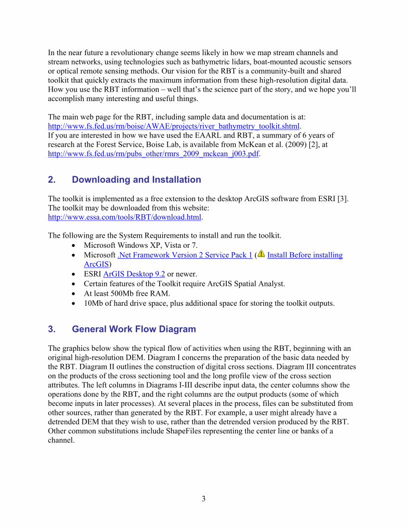
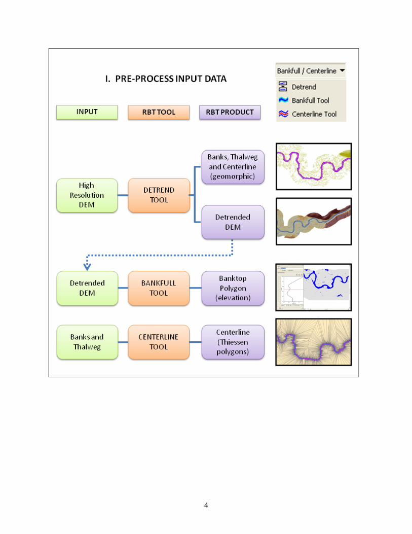
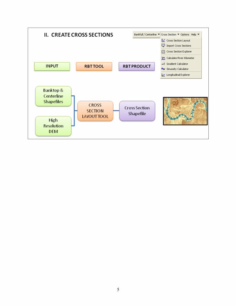
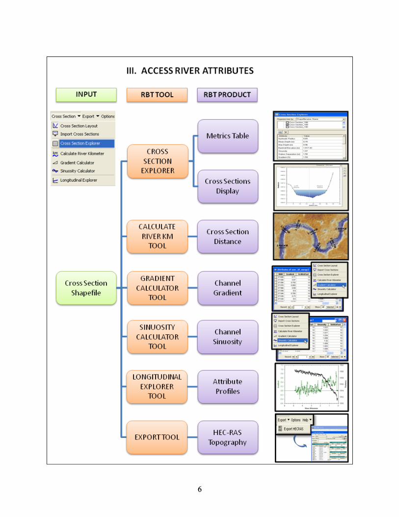
3. General Work Flow Diagram The graphics below show the typical flow of activities when using the RBT, beginning with an original high-resolution DEM. Diagram I concerns the preparation of the basic data needed by the RBT. Diagram II outlines the construction of digital cross sections. Diagram III concentrates on the products of the cross sectioning tool and the long profile view of the cross section attributes. The left columns in Diagrams I-III describe input data, the center columns show the operations done by the RBT, and the right columns are the output products (some of which become inputs in later processes). At several places in the process, files can be substituted from other sources, rather than generated by the RBT. For example, a user might already have a detrended DEM that they wish to use, rather than the detrended version produced by the RBT. Other common substitutions include ShapeFiles representing the center line or banks of a channel.
3
4
5
6 6
4. Tutorial Tasks
RBT Basics
Task 1 – Getting Started
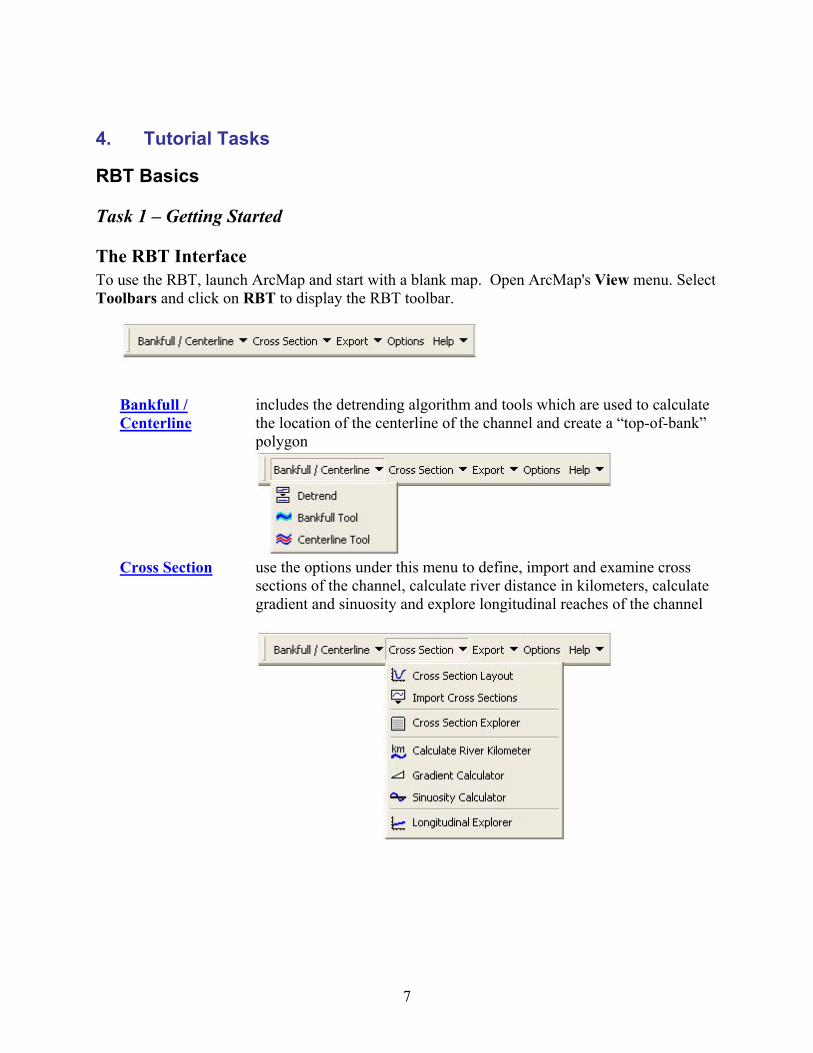
The RBT Interface To use the RBT, launch ArcMap and start with a blank map. Open ArcMap's View menu. Select Toolbars and click on RBT to display the RBT toolbar.
Bankfull / Centerline
includes the detrending algorithm and tools which are used to calculate the location of the centerline of the channel and create a “top-of-bank” polygon
Cross Section use the options under this menu to define, import and examine cross
sections of the channel, calculate river distance in kilometers, calculate gradient and sinuosity and explore longitudinal reaches of the channel
7
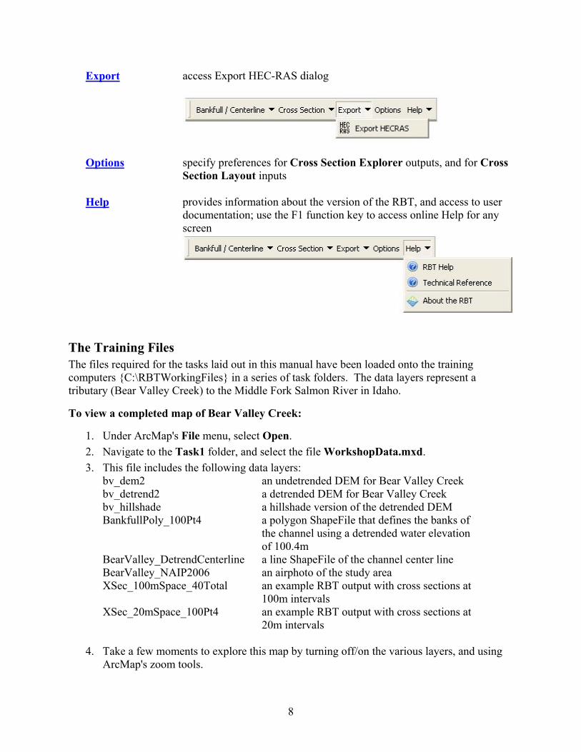
Export access Export HEC-RAS dialog
Options Help
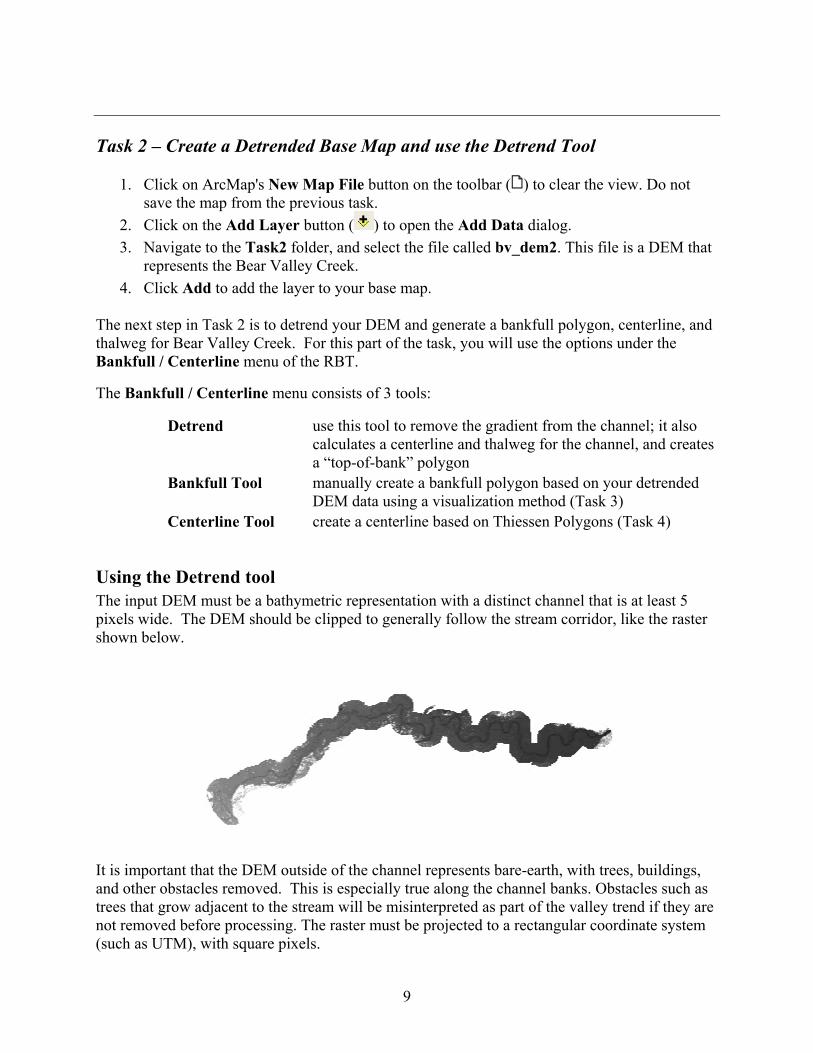
specify preferences for Cross Section Explorer outputs, and for Cross Section Layout inputs provides information about the version of the RBT, and access to user documentation; use the F1 function key to access online Help for any screen
The Training Files The files required for the tasks laid out in this manual have been loaded onto the training computers {C:\RBTWorkingFiles} in a series of task folders. The data layers represent a tributary (Bear Valley Creek) to the Middle Fork Salmon River in Idaho.
To view a completed map of Bear Valley Creek:
1. Under ArcMap's File menu, select Open. 2. Navigate to the Task1 folder, and select the file WorkshopData.mxd. 3. This file includes the following data layers:
bv_dem2 an undetrended DEM for Bear Valley Creek bv_detrend2 bv_hillshade
a detrended DEM for Bear Valley Creek a hillshade version of the detrended DEM
BankfullPoly_100Pt4 a polygon ShapeFile that defines the banks of the channel using a detrended water elevation of 100.4m
BearValley_DetrendCenterline BearValley_NAIP2006 XSec_100mSpace_40Total XSec_20mSpace_100Pt4
a line ShapeFile of the channel center line an airphoto of the study area an example RBT output with cross sections at 100m intervals an example RBT output with cross sections at 20m intervals
4. Take a few moments to explore this map by turning off/on the various layers, and using
ArcMap's zoom tools.
8
Task 2 – Create a Detrended Base Map and use the Detrend Tool
1. Click on ArcMap's New Map File button on the toolbar ( ) to clear the view. Do not save the map from the previous task.
2. Click on the Add Layer button ( ) to open the Add Data dialog. 3. Navigate to the Task2 folder, and select the file called bv_dem2. This file is a DEM that
represents the Bear Valley Creek. 4. Click Add to add the layer to your base map.
The next step in Task 2 is to detrend your DEM and generate a bankfull polygon, centerline, and thalweg for Bear Valley Creek. For this part of the task, you will use the options under the Bankfull / Centerline menu of the RBT.
The Bankfull / Centerline menu consists of 3 tools:
Detrend use this tool to remove the gradient from the channel; it also calculates a centerline and thalweg for the channel, and creates a “top-of-bank” polygon
Bankfull Tool manually create a bankfull polygon based on your detrended DEM data using a visualization method (Task 3)
Centerline Tool create a centerline based on Thiessen Polygons (Task 4)
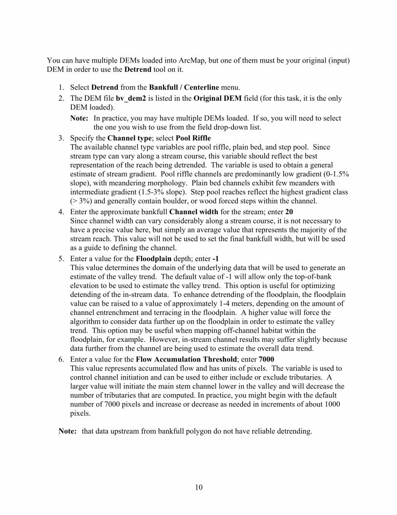
Using the Detrend tool The input DEM must be a bathymetric representation with a distinct channel that is at least 5 pixels wide. The DEM should be clipped to generally follow the stream corridor, like the raster shown below.
It is important that the DEM outside of the channel represents bare-earth, with trees, buildings, and other obstacles removed. This is especially true along the channel banks. Obstacles such as trees that grow adjacent to the stream will be misinterpreted as part of the valley trend if they are not removed before processing. The raster must be projected to a rectangular coordinate system (such as UTM), with square pixels.
9
You can have multiple DEMs loaded into ArcMap, but one of them must be your original (input) DEM in order to use the Detrend tool on it.
1. Select Detrend from the Bankfull / Centerline menu. 2. The DEM file bv_dem2 is listed in the Original DEM field (for this task, it is the only
DEM loaded). Note: In practice, you may have multiple DEMs loaded. If so, you will need to select
the one you wish to use from the field drop-down list. 3. Specify the Channel type; select Pool Riffle
The available channel type variables are pool riffle, plain bed, and step pool. Since stream type can vary along a stream course, this variable should reflect the best representation of the reach being detrended. The variable is used to obtain a general estimate of stream gradient. Pool riffle channels are predominantly low gradient (0-1.5% slope), with meandering morphology. Plain bed channels exhibit few meanders with intermediate gradient (1.5-3% slope). Step pool reaches reflect the highest gradient class (> 3%) and generally contain boulder, or wood forced steps within the channel.
4. Enter the approximate bankfull Channel width for the stream; enter 20 Since channel width can vary considerably along a stream course, it is not necessary to have a precise value here, but simply an average value that represents the majority of the stream reach. This value will not be used to set the final bankfull width, but will be used as a guide to defining the channel.
5. Enter a value for the Floodplain depth; enter -1 This value determines the domain of the underlying data that will be used to generate an estimate of the valley trend. The default value of -1 will allow only the top-of-bank elevation to be used to estimate the valley trend. This option is useful for optimizing detending of the in-stream data. To enhance detrending of the floodplain, the floodplain value can be raised to a value of approximately 1-4 meters, depending on the amount of channel entrenchment and terracing in the floodplain. A higher value will force the algorithm to consider data further up on the floodplain in order to estimate the valley trend. This option may be useful when mapping off-channel habitat within the floodplain, for example. However, in-stream channel results may suffer slightly because data further from the channel are being used to estimate the overall data trend.
6. Enter a value for the Flow Accumulation Threshold; enter 7000 This value represents accumulated flow and has units of pixels. The variable is used to control channel initiation and can be used to either include or exclude tributaries. A larger value will initiate the main stem channel lower in the valley and will decrease the number of tributaries that are computed. In practice, you might begin with the default number of 7000 pixels and increase or decrease as needed in increments of about 1000 pixels.
Note: that data upstream from bankfull polygon do not have reliable detrending.
10
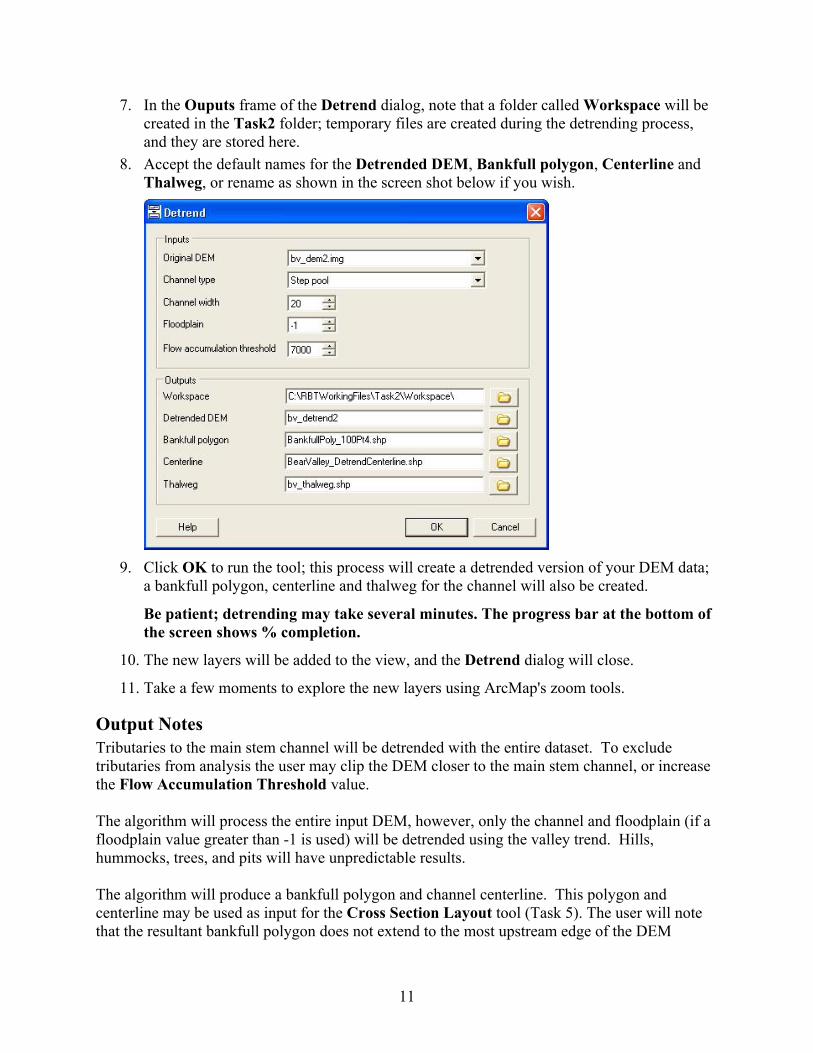
7. In the Ouputs frame of the Detrend dialog, note that a folder called Workspace will be created in the Task2 folder; temporary files are created during the detrending process, and they are stored here.
8. Accept the default names for the Detrended DEM, Bankfull polygon, Centerline and Thalweg, or rename as shown in the screen shot below if you wish.
9. Click OK to run the tool; this process will create a detrended version of your DEM data;
a bankfull polygon, centerline and thalweg for the channel will also be created.
Be patient; detrending may take several minutes. The progress bar at the bottom of the screen shows % completion.
10. The new layers will be added to the view, and the Detrend dialog will close.
11. Take a few moments to explore the new layers using ArcMap's zoom tools.
Output Notes Tributaries to the main stem channel will be detrended with the entire dataset. To exclude tributaries from analysis the user may clip the DEM closer to the main stem channel, or increase the Flow Accumulation Threshold value. The algorithm will process the entire input DEM, however, only the channel and floodplain (if a floodplain value greater than -1 is used) will be detrended using the valley trend. Hills, hummocks, trees, and pits will have unpredictable results. The algorithm will produce a bankfull polygon and channel centerline. This polygon and centerline may be used as input for the Cross Section Layout tool (Task 5). The user will note that the resultant bankfull polygon does not extend to the most upstream edge of the DEM
11

dataset. The upstream extent of the polygon can be adjusted with the Flow Accumulation Threshold variable. Important: Any data above the upstream extent of the bankfull polygon HAS NOT BEEN
DETRENDED. Only data within and along the bankfull polygon will have reasonable detrending results.
Task 3 – Use the Bankfull Tool to create a bankfull polygon
In Task 2, you used the Detrend Tool to automatically generate a bankfull polygon during the detrending process. In this task, you will use the Bankfull Tool (under the Bankfull / Centerline menu) to manually create a bankfull polygon based on your detrended DEM from Task 2. The tool uses a sliding scale that "floods" the detrended landscape to the bankfull elevation specified by the user. The bankfull elevation data can be visualized either as a histogram or as a volume:area graph, and then exported as a bankfull polygon shapefile ready for use with the RBT's cross section tools. The Bankfull Tool dialog is dockable, like the ArcMap Table of Contents. Note: the Spatial Analyst extension must be enabled (Tools | Extensions) for the Bankfull
Tool to work.
1. Under ArcMap's File menu, select Open.
2. Navigate to the Task3 folder, and select the file Task3.mxd. Click Open. Do not save the map from the previous task. The base map for Task 3 will load. The DEM for this task is the one you detrended in the last task.
3. Open the Bankfull / Centerline menu and select Bankfull Tool. The tool will open in the docked position; you may need to adjust the height of the window to have a better view of the Bankfull elevation histogram.
4. Your detrended DEM layer (bv_detrend2) will be selected as the Input (because it is the only layer loaded).
Note: In practice, you may have multiple detrended DEMs loaded. If so, you will need to select the one you wish to use from the field drop-down list.
5. The histogram in the Bankfull elevation frame represents the frequency with which each elevation is represented in the detrended data. Narrow the range around the maximum elevation by adjusting the values in the Min and Max fields at the bottom of the graph pane to 95 and 105; each time you change a value here, click outside the box to refresh the view.
Tip: detrended DEMs are centered on a value of 100
6. Move the slider on the left up or down and watch the degree of "flooding" change until the riverbed is clearly visible without too much overflow into the surrounding landscape. The red line on the histogram represents the current elevation. You can fine-tune the current elevation using the up/down arrows in the Current field (below the graph pane)
12
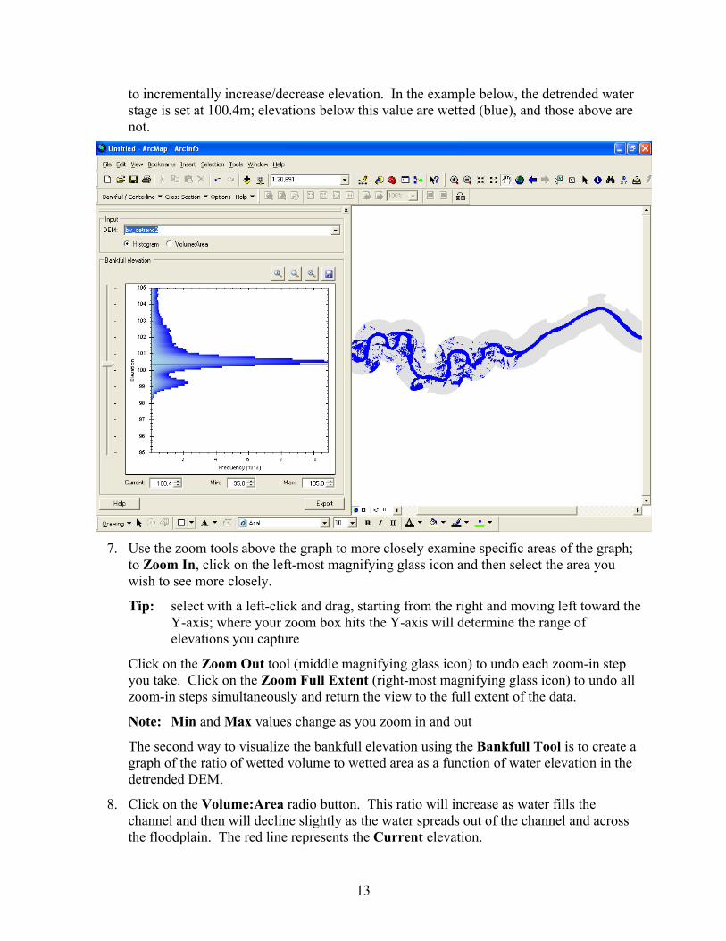
to incrementally increase/decrease elevation. In the example below, the detrended water stage is set at 100.4m; elevations below this value are wetted (blue), and those above are not.
7. Use the zoom tools above the graph to more closely examine specific areas of the graph;
to Zoom In, click on the left-most magnifying glass icon and then select the area you wish to see more closely.
Tip: select with a left-click and drag, starting from the right and moving left toward the Y-axis; where your zoom box hits the Y-axis will determine the range of elevations you capture
Click on the Zoom Out tool (middle magnifying glass icon) to undo each zoom-in step you take. Click on the Zoom Full Extent (right-most magnifying glass icon) to undo all zoom-in steps simultaneously and return the view to the full extent of the data.
Note: Min and Max values change as you zoom in and out
The second way to visualize the bankfull elevation using the Bankfull Tool is to create a graph of the ratio of wetted volume to wetted area as a function of water elevation in the detrended DEM.
8. Click on the Volume:Area radio button. This ratio will increase as water fills the channel and then will decline slightly as the water spreads out of the channel and across the floodplain. The red line represents the Current elevation.
13
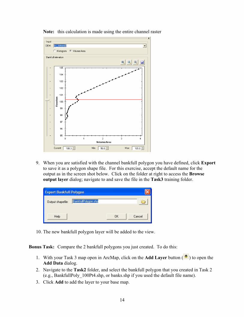
Note: this calculation is made using the entire channel raster
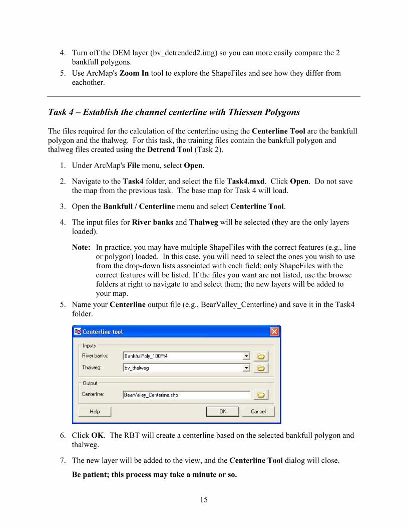
9. When you are satisfied with the channel bankfull polygon you have defined, click Export to save it as a polygon shape file. For this exercise, accept the default name for the output as in the screen shot below. Click on the folder at right to access the Browse output layer dialog; navigate to and save the file in the Task3 training folder.
10. The new bankfull polygon layer will be added to the view.
Bonus Task: Compare the 2 bankfull polygons you just created. To do this:
1. With your Task 3 map open in ArcMap, click on the Add Layer button ( ) to open the Add Data dialog.
2. Navigate to the Task2 folder, and select the bankfull polygon that you created in Task 2 (e.g., BankfullPoly_100Pt4.shp, or banks.shp if you used the default file name).
3. Click Add to add the layer to your base map.
14
4. Turn off the DEM layer (bv_detrended2.img) so you can more easily compare the 2 bankfull polygons.
5. Use ArcMap's Zoom In tool to explore the ShapeFiles and see how they differ from eachother.
Task 4 – Establish the channel centerline with Thiessen Polygons
The files required for the calculation of the centerline using the Centerline Tool are the bankfull polygon and the thalweg. For this task, the training files contain the bankfull polygon and thalweg files created using the Detrend Tool (Task 2).
1. Under ArcMap's File menu, select Open.
2. Navigate to the Task4 folder, and select the file Task4.mxd. Click Open. Do not save the map from the previous task. The base map for Task 4 will load.
3. Open the Bankfull / Centerline menu and select Centerline Tool.
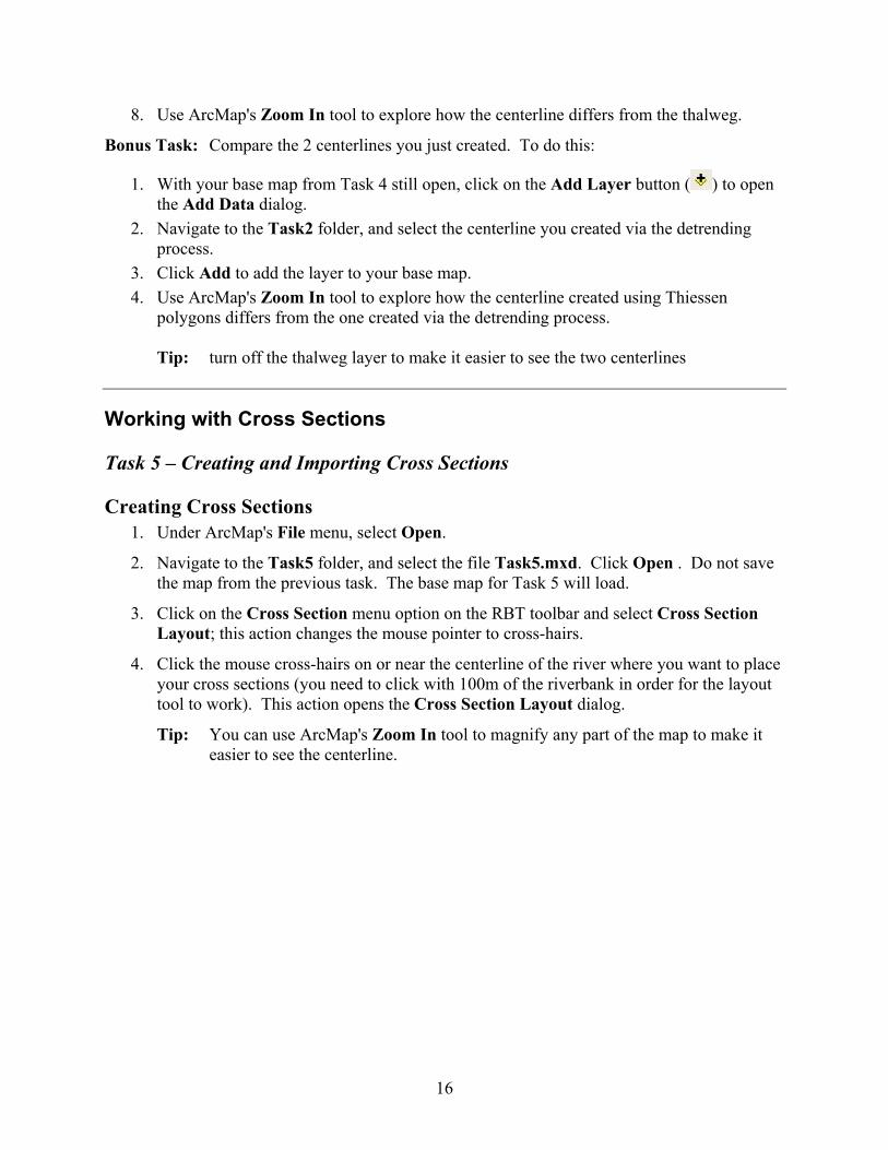
4. The input files for River banks and Thalweg will be selected (they are the only layers loaded).
Note: In practice, you may have multiple ShapeFiles with the correct features (e.g., line or polygon) loaded. In this case, you will need to select the ones you wish to use from the drop-down lists associated with each field; only ShapeFiles with the correct features will be listed. If the files you want are not listed, use the browse folders at right to navigate to and select them; the new layers will be added to your map.
5. Name your Centerline output file (e.g., BearValley_Centerline) and save it in the Task4 folder.
6. Click OK. The RBT will create a centerline based on the selected bankfull polygon and thalweg.
7. The new layer will be added to the view, and the Centerline Tool dialog will close.
Be patient; this process may take a minute or so.
15
8. Use ArcMap's Zoom In tool to explore how the centerline differs from the thalweg.
Bonus Task: Compare the 2 centerlines you just created. To do this:
1. With your base map from Task 4 still open, click on the Add Layer button ( ) to open the Add Data dialog.
2. Navigate to the Task2 folder, and select the centerline you created via the detrending process.
3. Click Add to add the layer to your base map. 4. Use ArcMap's Zoom In tool to explore how the centerline created using Thiessen
polygons differs from the one created via the detrending process.
Tip: turn off the thalweg layer to make it easier to see the two centerlines
Working with Cross Sections
Task 5 – Creating and Importing Cross Sections
Creating Cross Sections 1. Under ArcMap's File menu, select Open.
2. Navigate to the Task5 folder, and select the file Task5.mxd. Click Open . Do not save the map from the previous task. The base map for Task 5 will load.
3. Click on the Cross Section menu option on the RBT toolbar and select Cross Section Layout; this action changes the mouse pointer to cross-hairs.
4. Click the mouse cross-hairs on or near the centerline of the river where you want to place your cross sections (you need to click with 100m of the riverbank in order for the layout tool to work). This action opens the Cross Section Layout dialog.
Tip: You can use ArcMap's Zoom In tool to magnify any part of the map to make it easier to see the centerline.
16
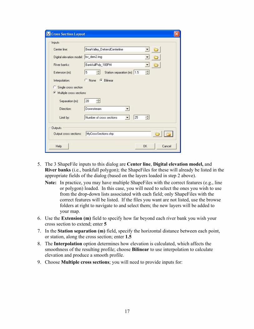
5. The 3 ShapeFile inputs to this dialog are Center line, Digital elevation model, and River banks (i.e., bankfull polygon); the ShapeFiles for these will already be listed in the appropriate fields of the dialog (based on the layers loaded in step 2 above). Note: In practice, you may have multiple ShapeFiles with the correct features (e.g., line
or polygon) loaded. In this case, you will need to select the ones you wish to use from the drop-down lists associated with each field; only ShapeFiles with the correct features will be listed. If the files you want are not listed, use the browse folders at right to navigate to and select them; the new layers will be added to your map.
6. Use the Extension (m) field to specify how far beyond each river bank you wish your cross section to extend; enter 5
7. In the Station separation (m) field, specify the horizontal distance between each point, or station, along the cross section; enter 1.5
8. The Interpolation option determines how elevation is calculated, which affects the smoothness of the resulting profile; choose Bilinear to use interpolation to calculate elevation and produce a smooth profile.
9. Choose Multiple cross sections; you will need to provide inputs for:
17
Separation (m) specify the distance, in meters, between the cross sections; enter 100
Direction specify whether you want the cross sections to be set upstream of where you initially clicked on your base map, downstream of that point, or both; make your selection from the drop-down list of options; select Downstream
Limit by the Distance option sets your cross sections over a specified length of the river - as many as will fit given the specified Separation (m) value and Direction; for this exercise, choose Number to create a set number of cross sections on the river over whatever distance is needed to achieve the specified Separation (m); for this task, enter 40
10. In the Outputs frame of the dialog, you can specify whether you want your cross section output to be appended to an existing line ShapeFile (see below) or saved to a new one.
11. For this exercise, create a new ShapeFile for your output using the following steps: • in the Outputs frame of the Cross Section Layout dialog, click on the new folder
icon to the far right of the Output cross sections field; this action opens a New Cross Section ShapeFile dialog
• click on the open folder icon to the right of the Output field; this action opens a Select location dialog; navigate to the training Task5 folder, and enter a name for the new ShapeFile in the Name field of the dialog (e.g., MyCrossSections)
• in the Import projection from field, select a ShapeFile that uses the same projection as the one you want to use for the new ShapeFile (either of the 2 listed can be chosen)
• click OK to return to the Cross Section Layout dialog
12. Click OK on the Cross Section Layout dialog to create your cross section(s) and see them displayed on your base map.
Be patient; this process may take a minute or so. The progress bar at the bottom of the screen shows % completion.
Alternatively, you could append your output to an existing ShapeFile. To do this:
• in the Outputs frame of the Cross Section Layout dialog, click on the open folder icon immediately to the right of the Output cross sections field; this action opens a Select Centre Line Feature Class dialog
• navigate to and select the line ShapeFile to which you wish to append your output • click Add to return to the Cross Section Layout dialog
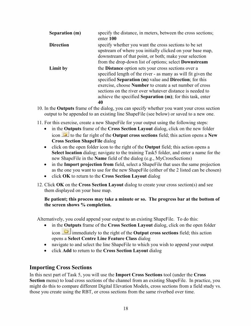
Importing Cross Sections In this next part of Task 5, you will use the Import Cross Sections tool (under the Cross Section menu) to load cross sections of the channel from an existing ShapeFile. In practice, you might do this to compare different Digital Elevation Models, cross sections from a field study vs. those you create using the RBT, or cross sections from the same riverbed over time.
18
1. With your Task 5 base map open in ArcMap, click on the Cross Section menu option on
the RBT toolbar and select Import Cross Sections. 2. From the Import cross sections drop-down list, select the ShapeFile that contains the
cross sections you just created (e.g., MyCrossSections). 3. The Digital elevation model and River banks fields will list your detrended DEM and
bankfull polygon respectively (these are the only ones loaded). Note: In practice, you may have multiple ShapeFiles with the correct features (e.g., line
or polygon) loaded. In this case, you will need to select the ones you wish to use from the drop-down lists associated with each field; only ShapeFiles with the correct features will be listed. If the files you want are not listed, use the browse folders at right to navigate to and select them; the new layers will be added to your map.
4. In the Station separation (m) field, specify the distance between points (or stations) along the cross section; enter 1.5
5. For Interpolation, choose None this time to create a set of cross sections without interpolation.
6. Use the Output 3D cross sections field to name your output file. Click on the folder at right and navigate to the training Task5 folder. Name the file (e.g., MyCrossSectionsNoInterpolation) and click Save to return to the Import Cross Sections dialog.
7. When you click OK on the Import Cross Sections dialog, the RBT will import the
specified cross section layer, and apply your Station separation and Interpolation instructions to it. The new layer will be given a name and location as indicated in the Output frame, and get added to your map.
19
Your base map now contains 2 sets of cross sections – one created with interpolation and the other without interpolation. Save the map using ArcMap's File|Save As option, calling it Task5_End.mxd. We will revisit this map in a later task to look at the effects of interpolation on cross section profiles.
Task 6 – Cross Section Explorer
In this task, you will use the Cross Section Explorer (under the Cross Section menu) to examine a set of cross sections in detail, including channel metrics and graphical profiles.
To explore cross section details:
1. Under ArcMap's File menu, select Open. 2. Navigate to the Task6 folder, and select the file Task6.mxd. Click Open and the base
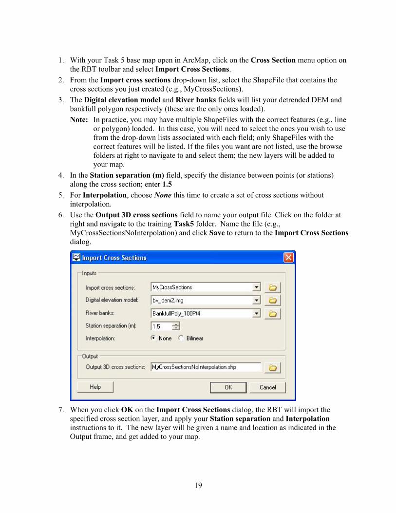
map for this task will load. 3. Select Cross Section Explorer from the RBT Cross Section menu to open the Cross
Section Explorer dialog. 4. Click on the + sign beside the ShapeFile name to expand the tree and see the list of cross
sections contained within it. There are 40 cross sections in this file.
20
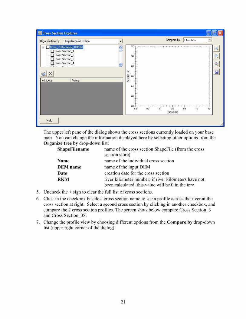
The upper left pane of the dialog shows the cross sections currently loaded on your base map. You can change the information displayed here by selecting other options from the Organize tree by drop-down list:
ShapeFilename name of the cross section ShapeFile (from the cross section store)
Name name of the individual cross section DEM name name of the input DEM Date creation date for the cross section RKM river kilometer number; if river kilometers have not
been calculated, this value will be 0 in the tree 5. Uncheck the + sign to clear the full list of cross sections. 6. Click in the checkbox beside a cross section name to see a profile across the river at the
cross section at right. Select a second cross section by clicking in another checkbox, and compare the 2 cross section profiles. The screen shots below compare Cross Section_3 and Cross Section_38.
7. Change the profile view by choosing different options from the Compare by drop-down list (upper right corner of the dialog).
21
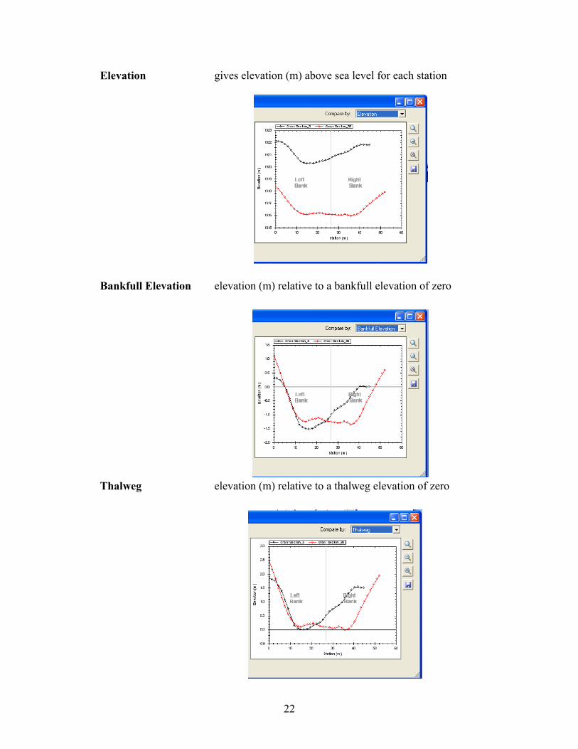
Elevation gives elevation (m) above sea level for each station
Bankfull Elevation elevation (m) relative to a bankfull elevation of zero
Thalweg elevation (m) relative to a thalweg elevation of zero
22
8. Use the zoom tools at far right to more closely examine specific areas of the profile. To
Zoom In, click on the uppermost magnifying glass icon and then select the area on the profile you wish to see more closely. Click on the Zoom Out tool (middle magnifying glass icon) to undo each zoom-in step you took. Click on the Zoom Full Extent (bottom magnifying glass icon) to undo all zoom-in steps simultaneously and return the view to the full extent of the data.
9. Save an image of the profile by clicking on the Save icon at far right; this action opens a Save As dialog. Navigate to the Task6 folder, and select the type of image file you want from the Save as type drop-down list (e.g., *.jpg). Give the file a name and click Save.
10. Zoom back out to the full extent of the data ( ).
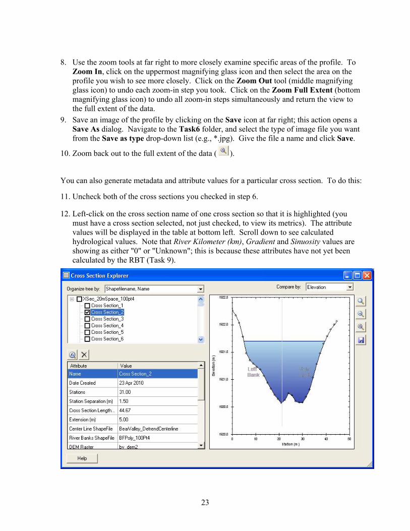
You can also generate metadata and attribute values for a particular cross section. To do this:
11. Uncheck both of the cross sections you checked in step 6.
12. Left-click on the cross section name of one cross section so that it is highlighted (you must have a cross section selected, not just checked, to view its metrics). The attribute values will be displayed in the table at bottom left. Scroll down to see calculated hydrological values. Note that River Kilometer (km), Gradient and Sinuosity values are showing as either "0" or "Unknown"; this is because these attributes have not yet been calculated by the RBT (Task 9).
23
The 2 buttons above the attribute data table are: Recalculate
re-calculates the hydrological attribute values, e.g., after changing an option (see about Options)
Clear
clears previously calculated hydrological attribute values
13. Close the Cross Section Explorer.
Task 7 – Elevation Interpolation
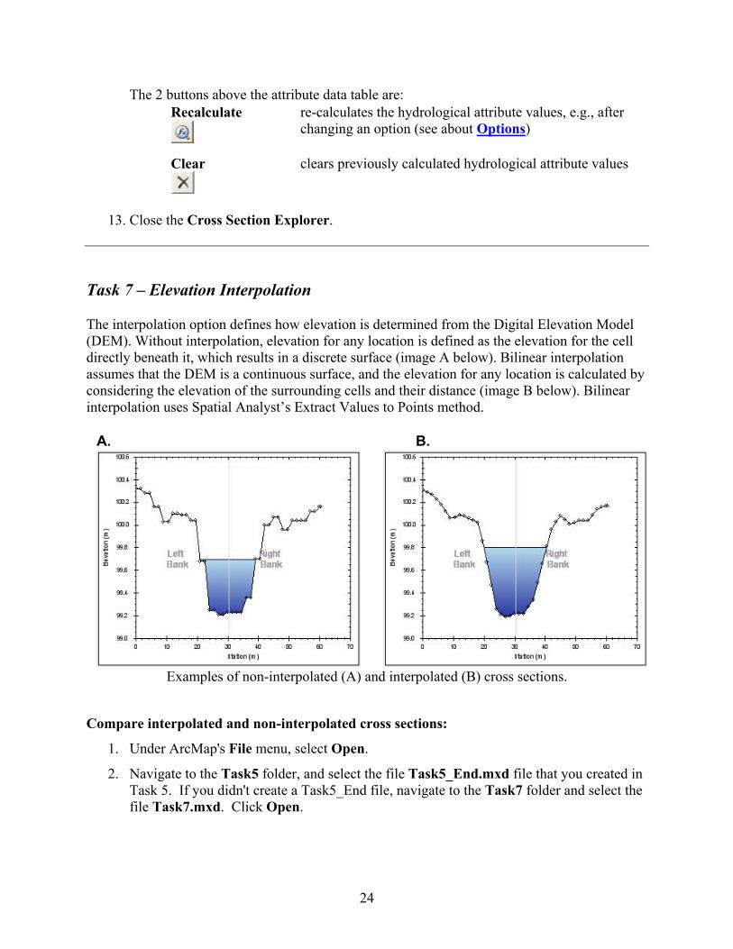
The interpolation option defines how elevation is determined from the Digital Elevation Model (DEM). Without interpolation, elevation for any location is defined as the elevation for the cell directly beneath it, which results in a discrete surface (image A below). Bilinear interpolation assumes that the DEM is a continuous surface, and the elevation for any location is calculated by considering the elevation of the surrounding cells and their distance (image B below). Bilinear interpolation uses Spatial Analyst’s Extract Values to Points method.
A. B.
Examples of non-interpolated (A) and interpolated (B) cross sections.
Compare interpolated and non-interpolated cross sections:
1. Under ArcMap's File menu, select Open.
2. Navigate to the Task5 folder, and select the file Task5_End.mxd file that you created in Task 5. If you didn't create a Task5_End file, navigate to the Task7 folder and select the file Task7.mxd. Click Open.
24
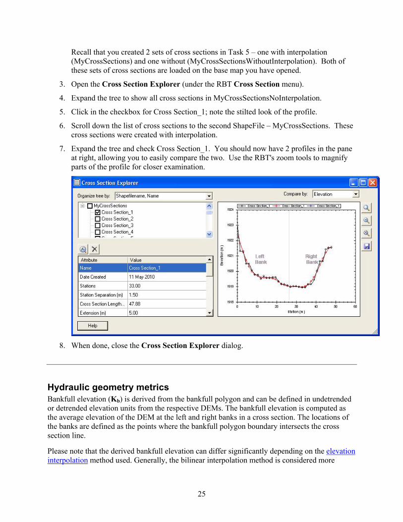
Recall that you created 2 sets of cross sections in Task 5 – one with interpolation (MyCrossSections) and one without (MyCrossSectionsWithoutInterpolation). Both of these sets of cross sections are loaded on the base map you have opened.
3. Open the Cross Section Explorer (under the RBT Cross Section menu).
4. Expand the tree to show all cross sections in MyCrossSectionsNoInterpolation.
5. Click in the checkbox for Cross Section_1; note the stilted look of the profile.
6. Scroll down the list of cross sections to the second ShapeFile – MyCrossSections. These cross sections were created with interpolation.
7. Expand the tree and check Cross Section_1. You should now have 2 profiles in the pane at right, allowing you to easily compare the two. Use the RBT's zoom tools to magnify parts of the profile for closer examination.
8. When done, close the Cross Section Explorer dialog.
Hydraulic geometry metrics Bankfull elevation (Kb) is derived from the bankfull polygon and can be defined in undetrended or detrended elevation units from the respective DEMs. The bankfull elevation is computed as the average elevation of the DEM at the left and right banks in a cross section. The locations of the banks are defined as the points where the bankfull polygon boundary intersects the cross section line.
Please note that the derived bankfull elevation can differ significantly depending on the elevation interpolation method used. Generally, the bilinear interpolation method is considered more
25
accurate, and is able to reproduce the elevation used to define the bankfull polygon using the bankfull tool on a detrended raster.
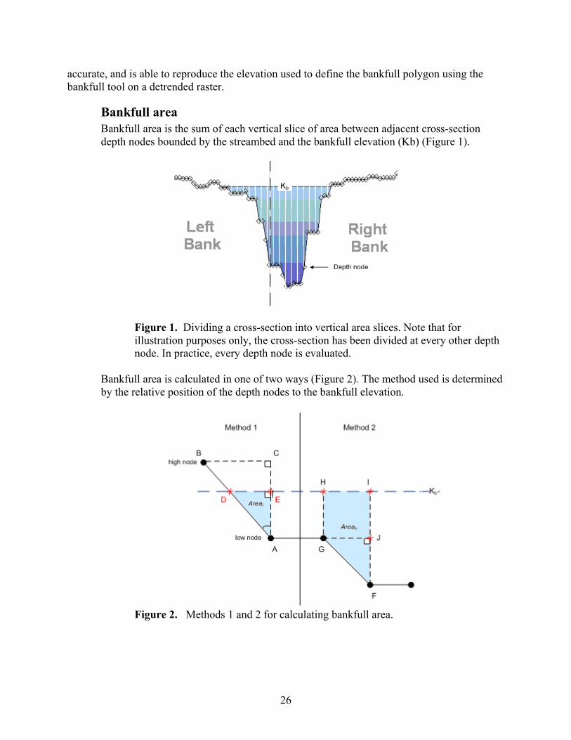
Bankfull area Bankfull area is the sum of each vertical slice of area between adjacent cross-section depth nodes bounded by the streambed and the bankfull elevation (Kb) (Figure 1).
Figure 1. Dividing a cross-section into vertical area slices. Note that for illustration purposes only, the cross-section has been divided at every other depth node. In practice, every depth node is evaluated.
Bankfull area is calculated in one of two ways (Figure 2). The method used is determined by the relative position of the depth nodes to the bankfull elevation.
Figure 2. Methods 1 and 2 for calculating bankfull area.
26
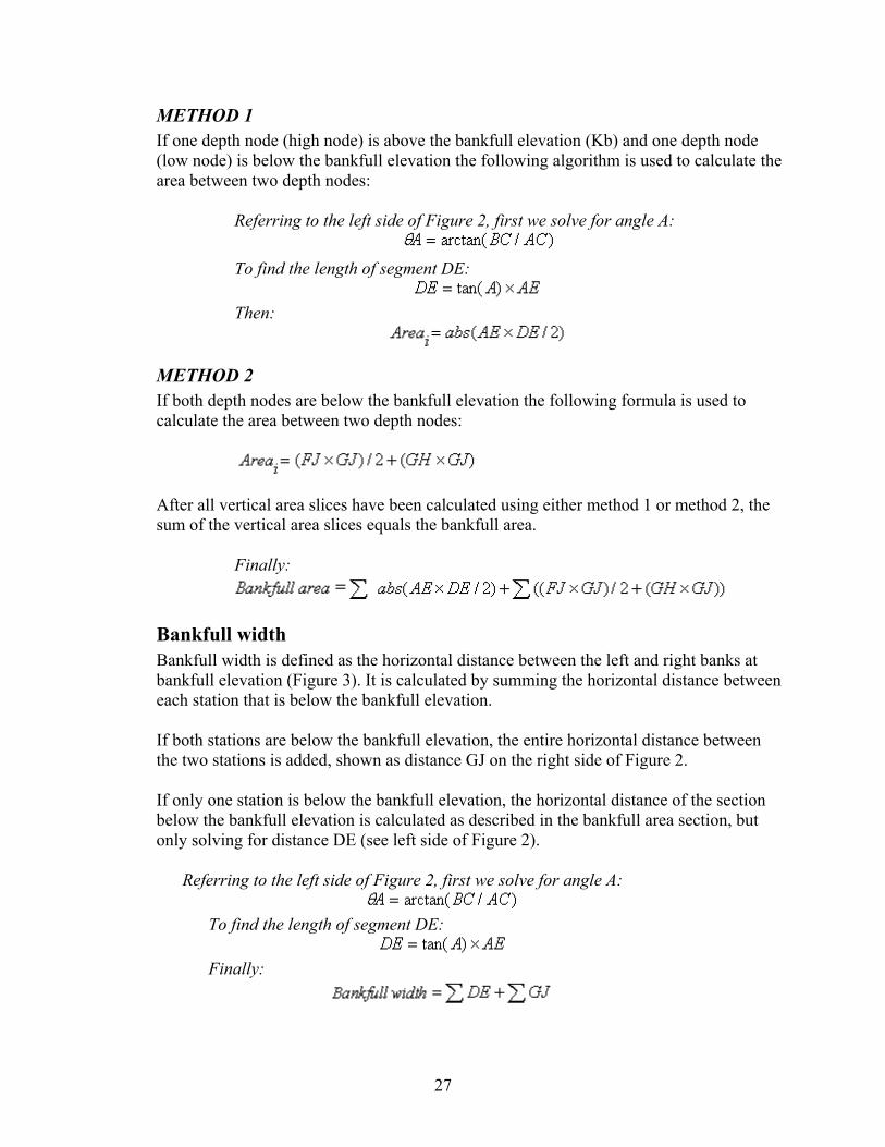
METHOD 1 If one depth node (high node) is above the bankfull elevation (Kb) and one depth node (low node) is below the bankfull elevation the following algorithm is used to calculate the area between two depth nodes:
Referring to the left side of Figure 2, first we solve for angle A:
To find the length of segment DE:
Then:
METHOD 2 If both depth nodes are below the bankfull elevation the following formula is used to calculate the area between two depth nodes:
After all vertical area slices have been calculated using either method 1 or method 2, the sum of the vertical area slices equals the bankfull area.
Finally:
Bankfull width Bankfull width is defined as the horizontal distance between the left and right banks at bankfull elevation (Figure 3). It is calculated by summing the horizontal distance between each station that is below the bankfull elevation. If both stations are below the bankfull elevation, the entire horizontal distance between the two stations is added, shown as distance GJ on the right side of Figure 2.
If only one station is below the bankfull elevation, the horizontal distance of the section below the bankfull elevation is calculated as described in the bankfull area section, but only solving for distance DE (see left side of Figure 2).
Referring to the left side of Figure 2, first we solve for angle A:
To find the length of segment DE:
Finally:
27
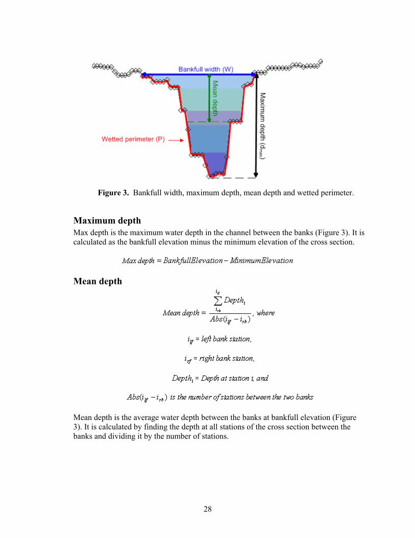
Figure 3. Bankfull width, maximum depth, mean depth and wetted perimeter.
Maximum depth Max depth is the maximum water depth in the channel between the banks (Figure 3). It is calculated as the bankfull elevation minus the minimum elevation of the cross section.
Mean depth
Mean depth is the average water depth between the banks at bankfull elevation (Figure 3). It is calculated by finding the depth at all stations of the cross section between the banks and dividing it by the number of stations.
28
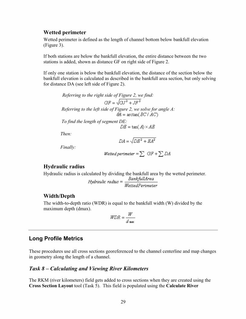
Wetted perimeter Wetted perimeter is defined as the length of channel bottom below bankfull elevation (Figure 3).
If both stations are below the bankfull elevation, the entire distance between the two stations is added, shown as distance GF on right side of Figure 2.
If only one station is below the bankfull elevation, the distance of the section below the bankfull elevation is calculated as described in the bankfull area section, but only solving for distance DA (see left side of Figure 2).
Referring to the right side of Figure 2, we find:
Referring to the left side of Figure 2, we solve for angle A:
To find the length of segment DE:
Then:
Finally:
Hydraulic radius Hydraulic radius is calculated by dividing the bankfull area by the wetted perimeter.
Width/Depth The width-to-depth ratio (WDR) is equal to the bankfull width (W) divided by the maximum depth (dmax).
Long Profile Metrics These procedures use all cross sections georeferenced to the channel centerline and map changes in geometry along the length of a channel.
Task 8 – Calculating and Viewing River Kilometers
The RKM (river kilometers) field gets added to cross sections when they are created using the Cross Section Layout tool (Task 5). This field is populated using the Calculate River
29
Kilometer tool (under the Cross Section menu). The RKM value identifies the location of each of your cross sections on the centerline relative to the downstream intersection of the centerline and the channel raster; if you add a value for Starting RKM (see below), then your RKM can be made relative to the mouth of the watercourse. The calculation is based on the point at which the cross section intersects the centerline. The RBT determines stream direction based on the elevation of each end of the centerline.
Calculating River Kilometers For calculating river kilometers for cross sections, you need a digital elevation model (to determine what is upstream and what is downstream), a centerline (to calculate distance from the starting point), and a set of cross sections (either imported or created using the RBT's cross section tools).
1. Under ArcMap's File menu, select Open.
2. Navigate to the Task8 folder, and select the file Task8.mxd. Click Open and the base map for this task will load. This file contains the layers you need to calculate river kilometers.
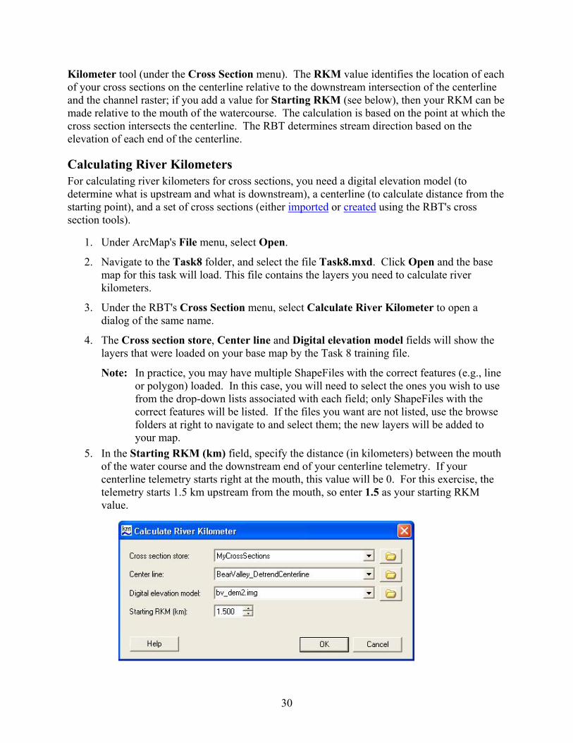
3. Under the RBT's Cross Section menu, select Calculate River Kilometer to open a dialog of the same name.
4. The Cross section store, Center line and Digital elevation model fields will show the layers that were loaded on your base map by the Task 8 training file.
Note: In practice, you may have multiple ShapeFiles with the correct features (e.g., line or polygon) loaded. In this case, you will need to select the ones you wish to use from the drop-down lists associated with each field; only ShapeFiles with the correct features will be listed. If the files you want are not listed, use the browse folders at right to navigate to and select them; the new layers will be added to your map.
5. In the Starting RKM (km) field, specify the distance (in kilometers) between the mouth of the water course and the downstream end of your centerline telemetry. If your centerline telemetry starts right at the mouth, this value will be 0. For this exercise, the telemetry starts 1.5 km upstream from the mouth, so enter 1.5 as your starting RKM value.
30
6. Click OK. The RBT will calculate the RKMs. 7. Leave your map open for the next part of this task.
Viewing the results of a river kilometer calculation You can view the river kilometers you have just calculated in different ways:
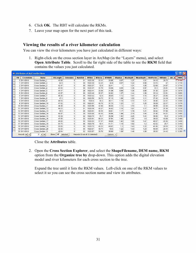
1. Right-click on the cross section layer in ArcMap (in the “Layers” menu), and select Open Attribute Table. Scroll to the far right side of the table to see the RKM field that contains the values you just calculated.
Close the Attributes table.
2. Open the Cross Section Explorer, and select the ShapeFilename, DEM name, RKM
option from the Organize tree by drop-down. This option adds the digital elevation model and river kilometers for each cross section to the tree.
Expand the tree until it lists the RKM values. Left-click on one of the RKM values to select it so you can see the cross section name and view its attributes.
31
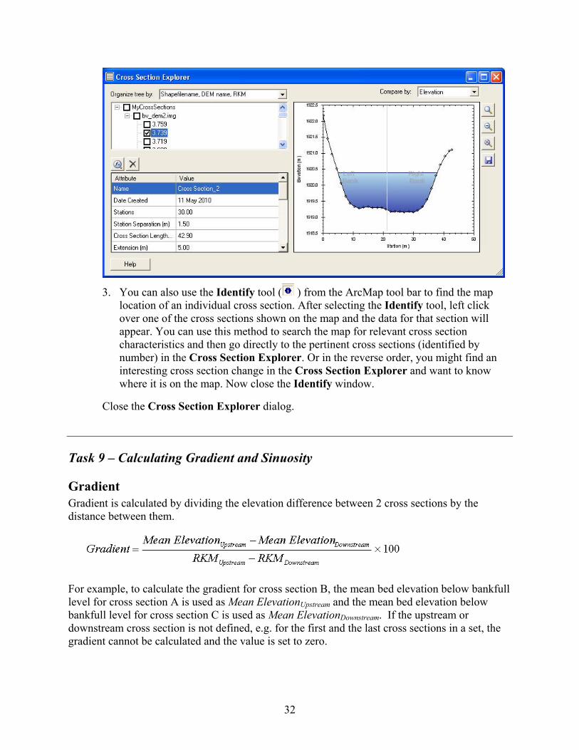
3. You can also use the Identify tool ( ) from the ArcMap tool bar to find the map
location of an individual cross section. After selecting the Identify tool, left click over one of the cross sections shown on the map and the data for that section will appear. You can use this method to search the map for relevant cross section characteristics and then go directly to the pertinent cross sections (identified by number) in the Cross Section Explorer. Or in the reverse order, you might find an interesting cross section change in the Cross Section Explorer and want to know where it is on the map. Now close the Identify window.
Close the Cross Section Explorer dialog.
Task 9 – Calculating Gradient and Sinuosity
Gradient Gradient is calculated by dividing the elevation difference between 2 cross sections by the distance between them.
For example, to calculate the gradient for cross section B, the mean bed elevation below bankfull level for cross section A is used as Mean ElevationUpstream and the mean bed elevation below bankfull level for cross section C is used as Mean ElevationDownstream. If the upstream or downstream cross section is not defined, e.g. for the first and the last cross sections in a set, the gradient cannot be calculated and the value is set to zero.
32
Calculating Gradient 1. Under ArcMap's File menu, select Open.
2. Navigate to the Task9 folder, and select the file Task9.mxd. Click Open and the base map for this task will load.
3. Select Gradient Calculator from the RBT Cross Section menu.
4. The Cross section store drop-down list will show the set of defined cross sections you will use for the calculation (it is the only one loaded for this task).
Note: In practice, you may have multiple cross section layers loaded. In this case, you will need to select the one you wish to use from the drop-down list. If the file you want is not listed, use the browse folders at right to navigate to and select it; the new layer will be added to your map.
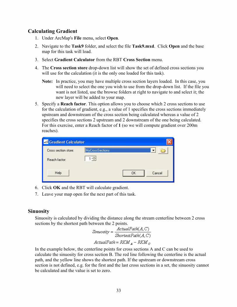
5. Specify a Reach factor. This option allows you to choose which 2 cross sections to use for the calculation of gradient, e.g., a value of 1 specifies the cross sections immediately upstream and downstream of the cross section being calculated whereas a value of 2 specifies the cross sections 2 upstream and 2 downstream of the one being calculated. For this exercise, enter a Reach factor of 1 (so we will compute gradient over 200m reaches).
6. Click OK and the RBT will calculate gradient. 7. Leave your map open for the next part of this task.
Sinuosity Sinuosity is calculated by dividing the distance along the stream centerline between 2 cross sections by the shortest path between the 2 points.
In the example below, the centerline points for cross sections A and C can be used to calculate the sinuosity for cross section B. The red line following the centerline is the actual path, and the yellow line shows the shortest path. If the upstream or downstream cross section is not defined, e.g. for the first and the last cross sections in a set, the sinuosity cannot be calculated and the value is set to zero.
33
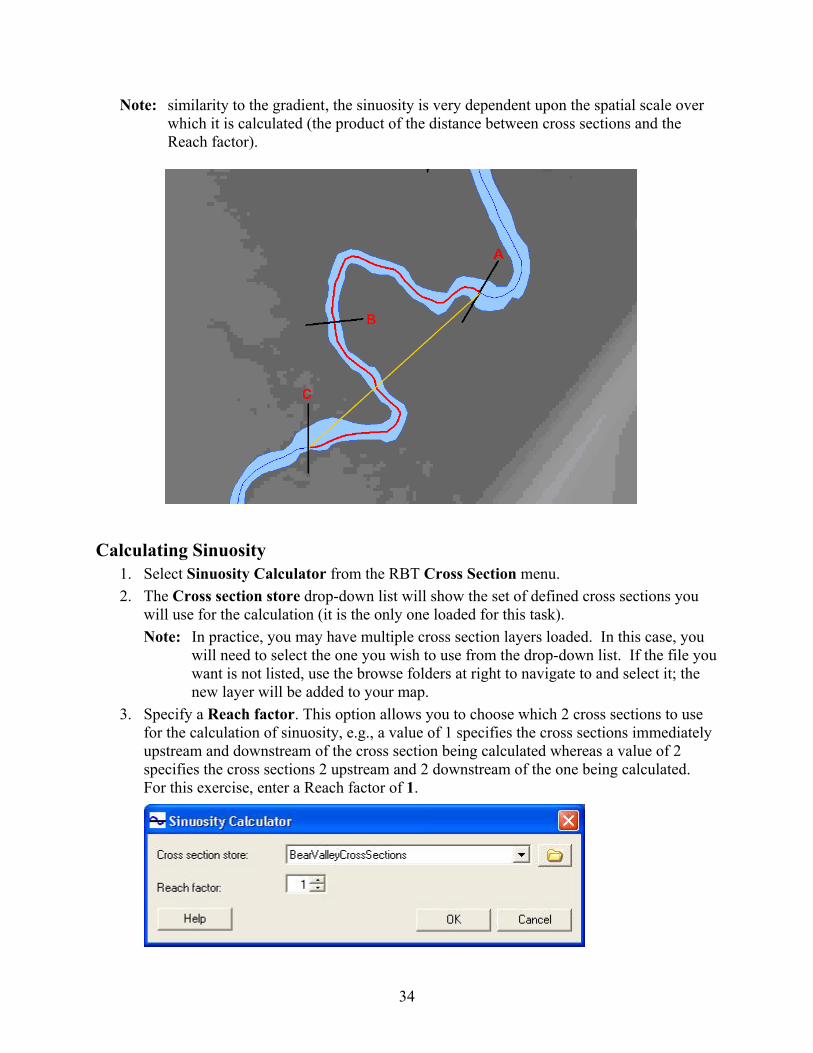
Note: similarity to the gradient, the sinuosity is very dependent upon the spatial scale over which it is calculated (the product of the distance between cross sections and the Reach factor).
Calculating Sinuosity ulator from the RBT Cross Section menu.
d cross sections you
ed. In this case, you
3. Specify u to choose which 2 cross sections to use
1. Select Sinuosity Calc2. The Cross section store drop-down list will show the set of define
will use for the calculation (it is the only one loaded for this task). Note: In practice, you may have multiple cross section layers load
will need to select the one you wish to use from the drop-down list. If the file youwant is not listed, use the browse folders at right to navigate to and select it; the new layer will be added to your map. a Reach factor. This option allows yo
for the calculation of sinuosity, e.g., a value of 1 specifies the cross sections immediatelyupstream and downstream of the cross section being calculated whereas a value of 2 specifies the cross sections 2 upstream and 2 downstream of the one being calculated.For this exercise, enter a Reach factor of 1.
34
4. Click OK and the RBT will calculate gradient.
Longitudinal Explorer Use the Longitudinal Explorer (under the Cross Section menu) to view a suite of attributes, based on a set of defined cross sections, along a stretch of the riverbed. Not so have river kilometers calculated for
them.
lick Open and the base
3. the Longitudinal Explorer (under the RBT Cross Sections menu).
t will show the set of defined cross sections you loaded).
cross section layers loaded. In this case, you
ed to your map. ribute will
.
yet, they will be unavailable (grayed
6. By defacheckb
e: The cross sections you use with this tool must al
Task 10 – Viewing riverbed attributes
1. Under ArcMap's File menu, select Open.
2. Navigate to the Task10 folder, and select the file Task10.mxd. Cmap for this task will load.
Launch
4. The Cross section store drop-down liswill use for this task (it is the only one
Note: In practice, you may have multiple will need to select the one you wish to use from the drop-down list. If the file you want is not listed, use the browse folders at right to navigate to and select it; the new layer will be add
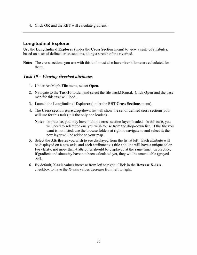
5. Select the Attributes you wish to see displayed from the list at left. Each attbe displayed on a new axis, and each attribute axis title and line will have a unique colorFor clarity, not more than 4 attributes should be displayed at the same time. In practice,if gradient and sinuosity have not been calculatedout).
ult, X-axis values increase from left to right. Click in the Reverse X-axis ox to have the X-axis values decrease from left to right.
35
7. Use the zoom tools at the top of the dialog to more closely examine specific areas of the
graph. To Zoom In, click on the leftmost magnifying glass icon and then select the area on the graph you wish to see more closely. Click on the Zoom Out tool (middle magnifying glass icon) to undo each zoom-in step you take. Click on the Zoom Full Extent (bottom magnifying glass icon) to undo all zoom-in steps simultaneously and return the view to the full extent of the data.
8. Save an image of the graph by clicking on the Save icon in the upper right corner of the dialog. This action opens a Save As dialog; navigate to the training Task10 folder, select the type of image you wish to save, and give the file a name. Click Save to save the file and return to the Longitudinal Explorer dialog.
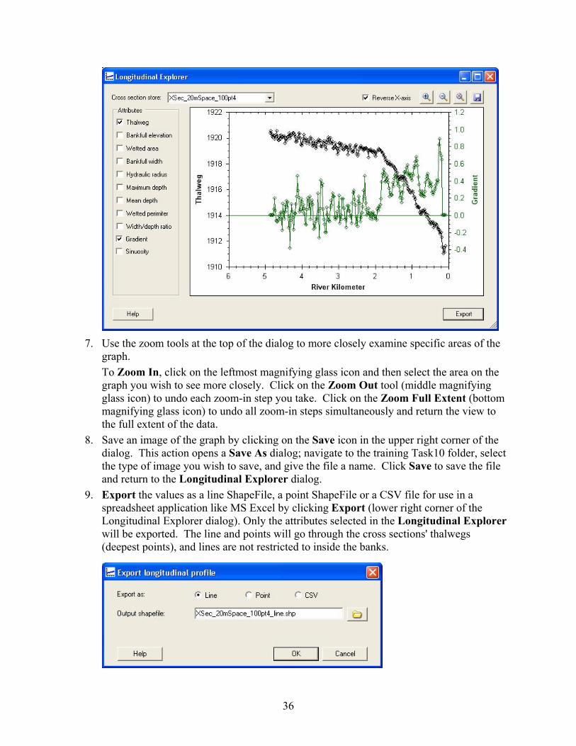
9. Export the values as a line ShapeFile, a point ShapeFile or a CSV file for use in a spreadsheet application like MS Excel by clicking Export (lower right corner of the Longitudinal Explorer dialog). Only the attributes selected in the Longitudinal Explorer will be exported. The line and points will go through the cross sections' thalwegs (deepest points), and lines are not restricted to inside the banks.
36

10. Click OK to export the data. Close the Longitudinal Explorer dialog.
Task 11 – Export to HEC-RAS
The Export HECRAS feature of the RBT exports spatial data in a form that can be imported into an external program called HEC-RAS to model in one dimension the hydraulics of water flow through natural rivers and other channels.
1. Under ArcMap's File menu, select Open.
2. Navigate to the Task11 folder, and select the file Task11.mxd. Click Open and the base map for this task will load.
3. Open the HEC-RAS Export dialog (under the RBT Export menu).
The inputs to this dialog include a centerline, a bankfull polygon and a set of cross sections.
4. The file BearValley_DetrendCenterline will be listed in the Center line field, and the file BankfullPoly_100Pt4 will be listed in the River banks field (these are the only ShapeFiles with the Task11 base map). Note: In practice, you may have multiple ShapeFiles with the correct features (e.g., line
or polygon) loaded. In this case, you will need to select the ones you wish to use from the drop-down lists associated with each field; only ShapeFiles with the correct features will be listed. If the files you want are not listed, use the browse folders at right to navigate to and select them; the new layers will be added to your map.
5. Open the Cross section store drop-down list, and select the set of cross sections you wish to export.
6. Enter Manning's N values for Bear Valley Creek. The Manning Equation is commonly used for analyzing open channel flows, and is integral to the HEC-RAS model. Manning's N values define resistance to flow for the main Channel, the left overbank (LOB) and the right overbank (ROB). Use Manning’s values of .06 for LOB and ROB and .04 for the Channel (see the screen shot below).
The output from the export process is a file that can be imported into HEC-RAS for analysis of channel hydraulics.
7. In the Output frame of the HEC-RAS Export dialog, click on the Export file browse folder to open a Browse output layer dialog. Navigate to the Task11 training folder, and give your output file a name. Click Save to return to the HEC-RAS Export dialog.
37
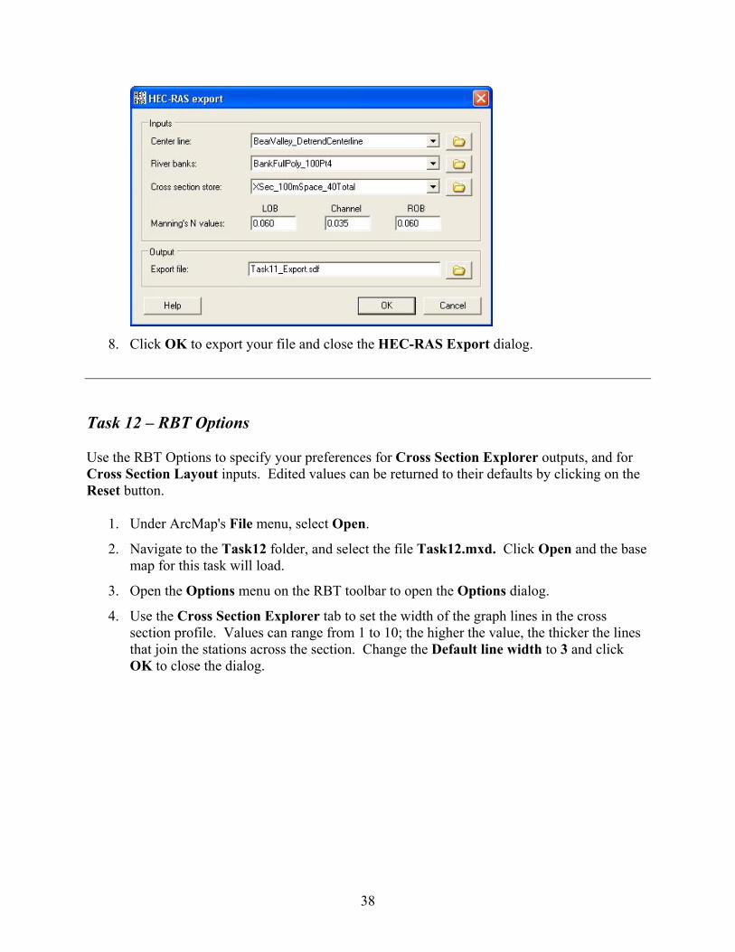
8. Click OK to export your file and close the HEC-RAS Export dialog.
Task 12 – RBT Options
Use the RBT Options to specify your preferences for Cross Section Explorer outputs, and for Cross Section Layout inputs. Edited values can be returned to their defaults by clicking on the Reset button.
1. Under ArcMap's File menu, select Open.
2. Navigate to the Task12 folder, and select the file Task12.mxd. Click Open and the base map for this task will load.
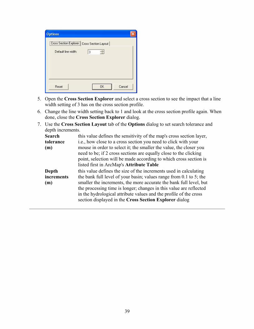
3. Open the Options menu on the RBT toolbar to open the Options dialog.
4. Use the Cross Section Explorer tab to set the width of the graph lines in the cross section profile. Values can range from 1 to 10; the higher the value, the thicker the lines that join the stations across the section. Change the Default line width to 3 and click OK to close the dialog.
38
5. Open the Cross Section Explorer and select a cross section to see the impact that a line
width setting of 3 has on the cross section profile. 6. Change the line width setting back to 1 and look at the cross section profile again. When
done, close the Cross Section Explorer dialog. 7. Use the Cross Section Layout tab of the Options dialog to set search tolerance and
depth increments. Search tolerance (m)
this value defines the sensitivity of the map's cross section layer, i.e., how close to a cross section you need to click with your mouse in order to select it; the smaller the value, the closer you need to be; if 2 cross sections are equally close to the clicking point, selection will be made according to which cross section is listed first in ArcMap's Attribute Table
Depth increments (m)
this value defines the size of the increments used in calculating the bank full level of your basin; values range from 0.1 to 5; the smaller the increments, the more accurate the bank full level, but the processing time is longer; changes in this value are reflected in the hydrological attribute values and the profile of the cross section displayed in the Cross Section Explorer dialog
39
5. Glossary of Terms
Bankfull – Generally defined in the RBT as the elevation corresponding to the intersection of a floodplain and the top edge of the channel banks; i.e. if the water surface was higher than bankfull, water would escape the channel and begin to flow onto a floodplain. RBT provides two methods to determine the top of the bank (Bankfull Tool and Banks.shp from the Detrending process) and accommodates other definitions by allowing user-created bankfull polygons.
Bilinear Interpolation – An Arc GIS tool which uses the value of the four nearest input cell centers to determine the value on the output raster. The new value for the output cell is a weighted average of these four values, adjusted to account for their distance from the center of the output cell. Output which is not interpolated uses the value at the center of the cell.
Centerline – The line which runs longitudinally down the middle of the polygon used to define the top of banks or bankfull.
Cross Section – A profile line placed perpendicular to the centerline.
DEM – Digital Elevation Model. Typically, this is a raster representing surface elevations.
Detrend - Remove the larger scale slope of a valley or channel while maintaining the local topographic features such as channel pools and bank breaks. The detrended data are referenced to an artificial datum, with the bankfull elevation near 100m.
Extension – Distance the cross sections will extend onto the floodplain past the top of bank.
Gradient – The slope of the channel bottom over a user-defined distance.
Longitudinal Profile – A profile of an attribute, such as width/depth ratio, as it changes along the centerline.
Reach Factor – Defines the length of channel used to calculate gradient and sinuosity. The Reach Factor is the number of cross sections above and below the target cross section that will be used to determine the reach of stream in the calculation. Reach Factor = 1 will calculate gradient or sinuosity for the channel between the cross sections directly above and below the target cross section. Reach Factor = 2 will calculate gradient or sinuosity using endpoints that are 2 cross sections above the target and 2 cross sections below the target. Increasing the reach factor lengthens the run over which the metric is calculated.
River Kilometer – The distance upstream along the centerline. RBT assigns 0 to the starting distance at the downstream end of the centerline, but the user can “offset” the starting distance to account for the distance between the centerline and the mouth of the watercourse or any other benchmark, if desired.
Separation – The longitudinal distance between cross sections.
Sinuosity – A description of the degree of meandering of a stream channel, calculated over any user-defined channel length.
40

6. References [1] HEC-RAS website. Available online: http://www.hec.asce.army.mil/software/hec-ras/
[2] McKean, J., Nagel, D., Tonina, D., Bailey, P., Wright, C.W., Bohn, C., Nayegandhi, A., 2009. Remote sensing of channels and riparian zones with a narrow-beam aquatic-terrestrial lidar. Remote Sensing, 1, 1065-1096; doi:10.3390/rs1041065
[3] ArcGIS 9.3 website. Available online: http://www.esri.com/software/arcgis/index.html
41