Embed Size (px)
Citation preview

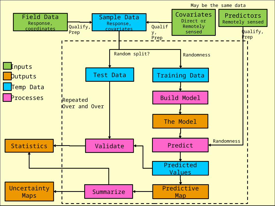
Sample DataResponse, covariates
PredictorsRemotely sensed
Build Model
Uncertainty Maps
CovariatesDirect or Remotely
sensed
Training DataTest Data
Predictive Map
The Model
Statistics
Qualify, Prep
Qualify,Prep Qualify,
Prep
Predict
Summarize
Predicted Values
ValidateRandomness
Randomness
Inputs
Outputs
RepeatedOver and Over
Field DataResponse, coordinates
Processes
Temp Data
Random split?
May be the same data
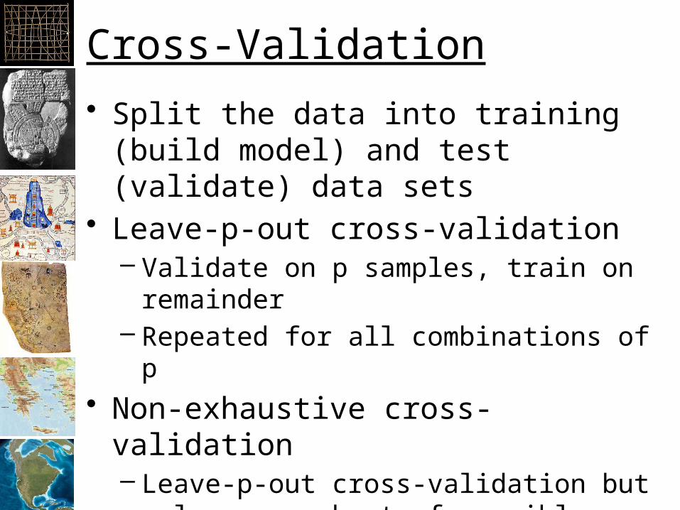
Cross-Validation
• Split the data into training (build model) and test (validate) data sets
• Leave-p-out cross-validation– Validate on p samples, train on remainder– Repeated for all combinations of p
• Non-exhaustive cross-validation– Leave-p-out cross-validation but only on a
subset of possible combinations– Randomly splitting into 30% test and 70%
training is common
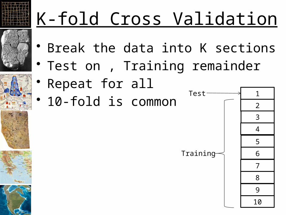
K-fold Cross Validation
• Break the data into K sections• Test on , Training remainder• Repeat for all • 10-fold is common
1
2
3
4
5
6
7
8
9
10
Training
Test
Bootstrapping
• Drawing N samples from the sample data (with replacement)
• Building the model• Repeating the process over and over
Random Forest
• N samples drawn from the data with replacement
• Repeated to create many trees– A “random forest”
• “Splits” are selected based on the most common splits in all the trees
• Bootstrap aggregation or “Bagging”
Boosting
• Can a set of weak learners create a single strong learner? (Wikipedia)– Lots of “simple” trees used to create a really
complex tree• "convex potential boosters cannot
withstand random classification noise,“– 2008 Phillip Long (at Google) and Rocco A.
Servedio (Columbia University)
Boosted Regression Trees
• BRTs combine thousands of trees to reduce deviance from the data
• Currently popular• More on this later
Sensitivity Testing
• Injecting small amounts of “noise” into our data to see the effect on the model parameters.– Plant
• The same approach can be used to model the impact of uncertainty on our model outputs and to make uncertainty maps
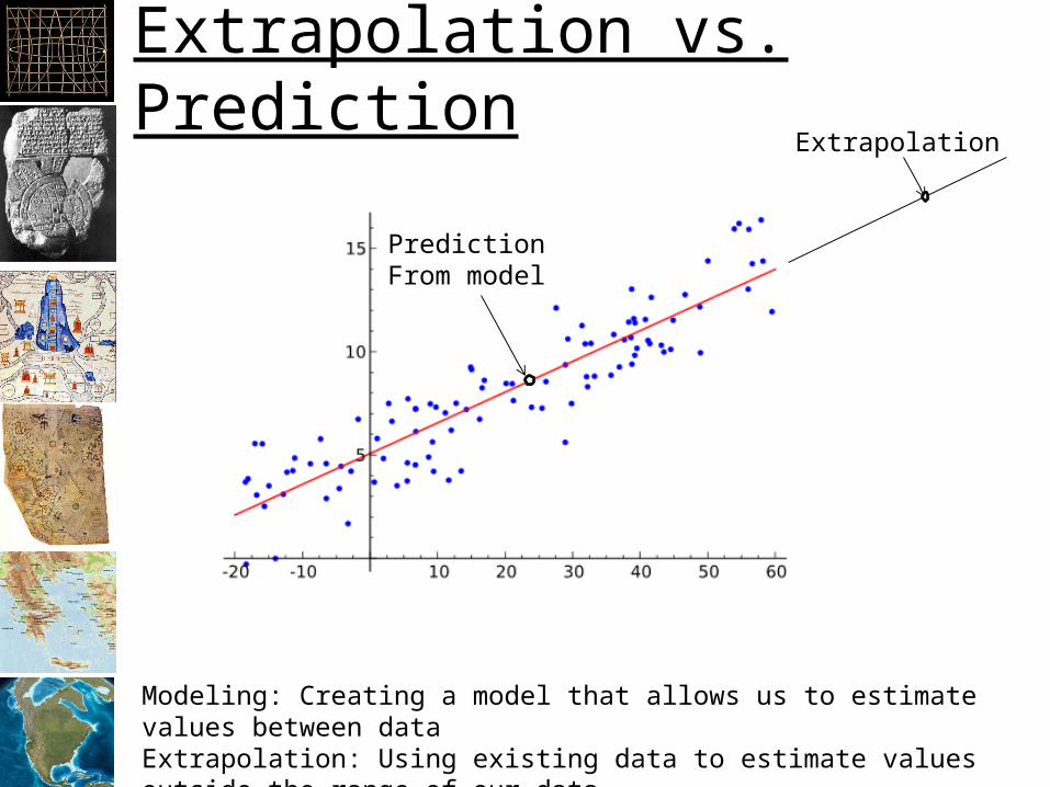
Extrapolation vs. Prediction
Modeling: Creating a model that allows us to estimate values between dataExtrapolation: Using existing data to estimate values outside the range of our data
Extrapolation
PredictionFrom model
Building Models
• Selecting the method• Selecting the predictors (“Model
Selection”)• Optimizing the coefficients/parameters of
the model
Response Drives Method
• Occurrences: Maxent, HEMI• Binary: GLM with logistic• Categorical: Classification Tree• Counts: GLM with Poisson• Continuous:
– Linear for linear– GLM with Gamma for distances– GAM for others
• Can convert between types when required and appropriate
Occurrences to:• Binary:
– Create a count data set as below – Use the field calculator to convert values >0
to 1 • Count:
– Take one of your predictor variable rasters and convert it to a polygon mesh
– Add an attribute that counts the number of occurrences in each polygon
• Continuous: – Convert your point data set to a density
raster, then convert the raster to points
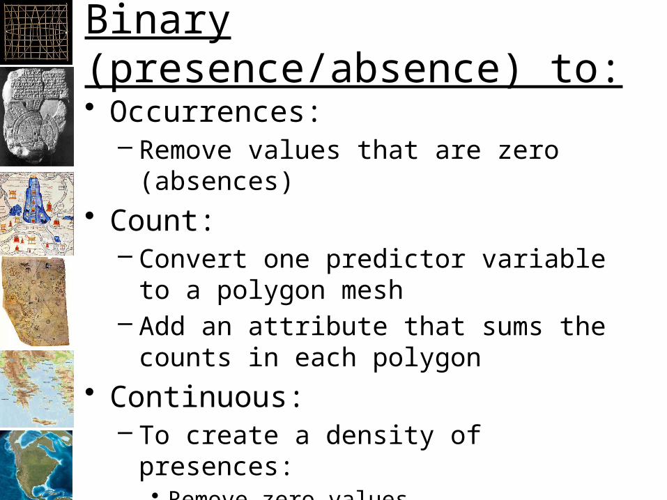
Binary (presence/absence) to:
• Occurrences: – Remove values that are zero (absences)
• Count: – Convert one predictor variable to a polygon
mesh– Add an attribute that sums the counts in
each polygon• Continuous:
– To create a density of presences: • Remove zero values• Convert point data to density raster
– To create a mean value: • Convert one predictor variable to a polygon
mesh• Add an attribute that counts the number of
presence points in each polygon• Add an attribute that counts the number of
absences in each polygon
– Find the mean of the presence count and the absence count

Binary (presence/absence) to:
• Continuous: – To create a density of presences:
• Remove zero values• Convert point data to density raster
– To create a mean value: • Convert one predictor variable to a polygon
mesh• Add an attribute that counts the number of
presence points in each polygon• Add an attribute that counts the number of
absences in each polygon• Find the mean of the presence count and the
absence count?
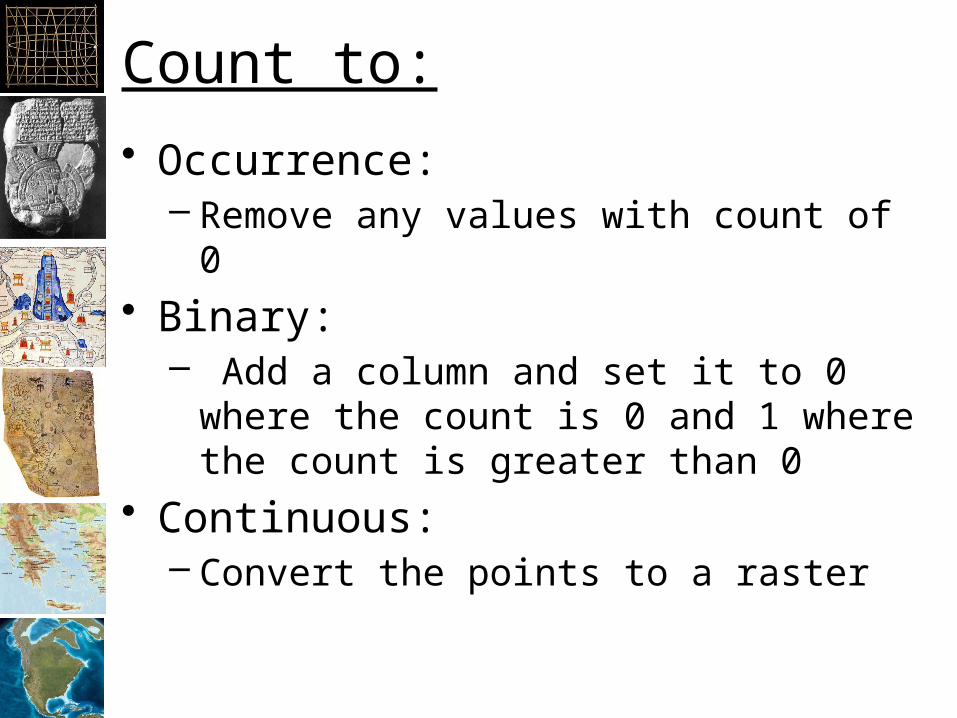
Count to:
• Occurrence: – Remove any values with count of 0
• Binary:– Add a column and set it to 0 where the
count is 0 and 1 where the count is greater than 0
• Continuous: – Convert the points to a raster
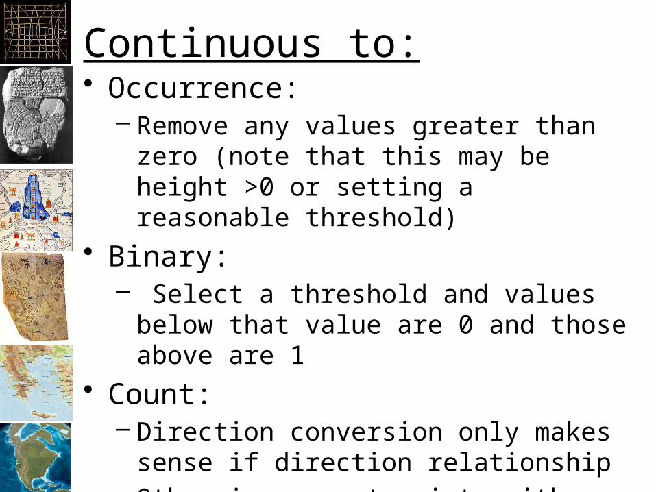
Continuous to:• Occurrence:
– Remove any values greater than zero (note that this may be height >0 or setting a reasonable threshold)
• Binary:– Select a threshold and values below that
value are 0 and those above are 1• Count:
– Direction conversion only makes sense if direction relationship
– Otherwise, count points with attribute > value
Sample DataResponse, covariates
PredictorsRemotely sensed
Build Model
Uncertainty Maps
CovariatesDirect or Remotely
sensed
Training DataTest Data
Predictive Map
The Model
Statistics
Qualify, Prep
Qualify,Prep Qualify,
Prep
Predict
Summarize
Predicted Values
ValidateRandomness
Randomness
Inputs
Outputs
RepeatedOver and Over
Field DataResponse, coordinates
Processes
Temp Data
Random split?
May be the same data
Model Selection
• Need a method to select the “best” set of predictors – Really to select the best method, predictors,
and coefficients (parameters)• Should be a balance between fitting the
data and simplicity– R2 – only considers fit to data (but linear
regression is pretty simple)

Simplicity
• Everything should be made as simple as possible, but not simpler.– Albert Einstein
"Albert Einstein Head" by Photograph by Oren Jack Turner, Princeton, licensed through Wikipedia
Parsimony
• “…too few parameters and the model will be so unrealistic as to make prediction unreliable, but too many parameters and the model will be so specific to the particular data set so to make prediction unreliable.”– Edwards, A. W. F. (2001). Occam’s bonus. p. 128–
139; in Zellner, A., Keuzenkamp, H. A., and McAleer, M. Simplicity, inference and modelling. Cambridge University Press, Cambridge, UK.
Parsimony
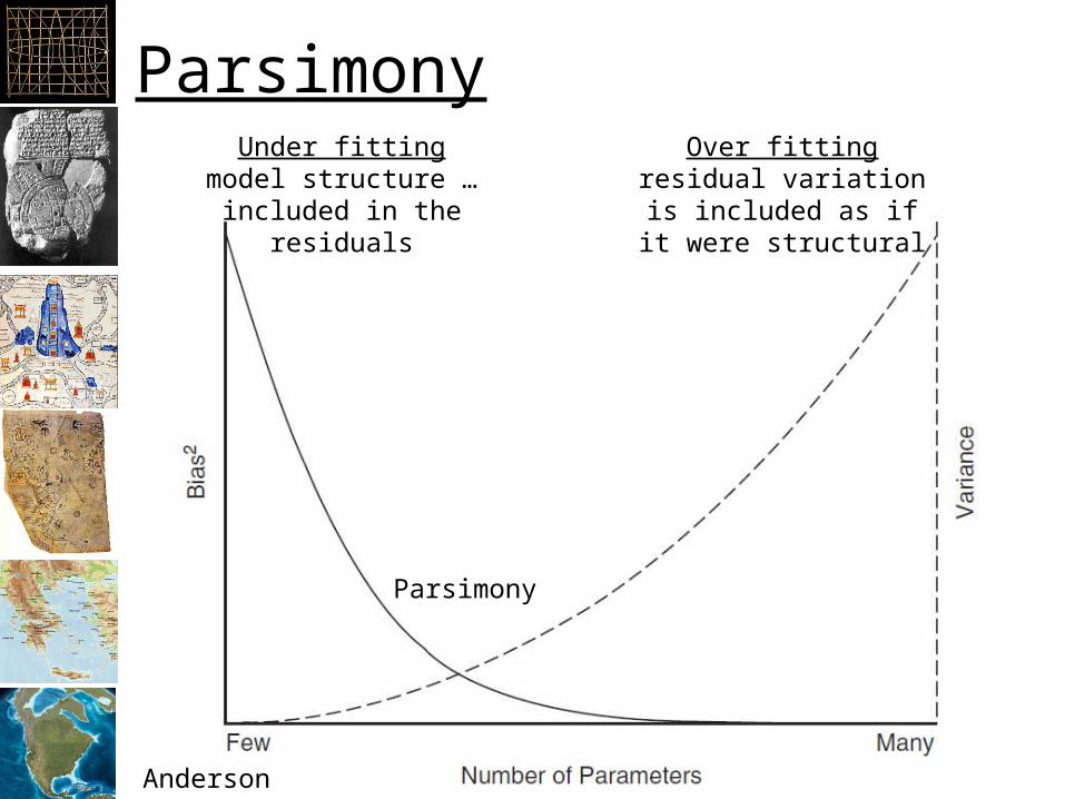
Anderson
Under fittingmodel structure …
included in theresiduals
Over fittingresidual variation
is included as if it were structural
Parsimony
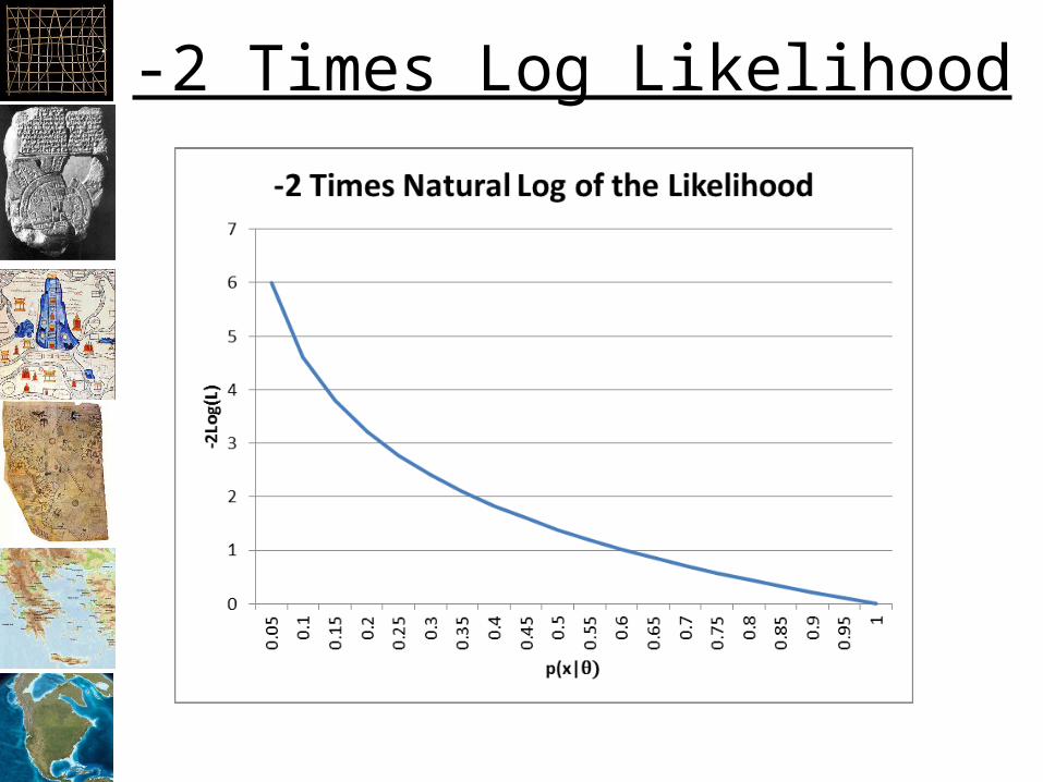
Akaike Information Criterion
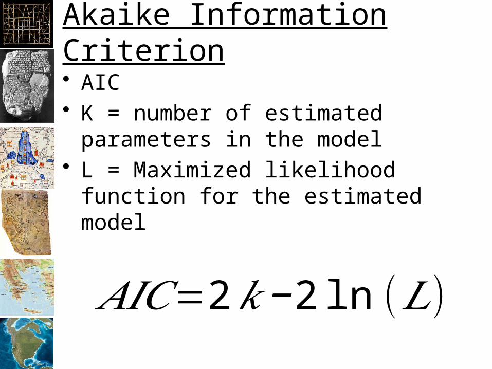
• AIC• K = number of estimated parameters in
the model• L = Maximized likelihood function for the
estimated model
𝐴𝐼𝐶=2𝑘−2 ln (𝐿)
AIC
• Only a relative meaning• Smaller is “better”• Balance between complexity:
– Over fitting or modeling the errors– Too many parameters
• And bias– Under fitting or the model is missing part of
the phenomenon we are trying to model– Too few parameters
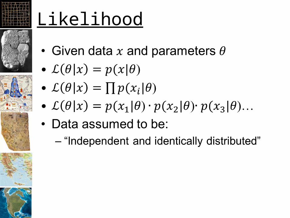
Likelihood
• Likelihood of a set of parameter values given some observed data=probability of observed data given parameter values
• Definitions– all sample values– one sample value– set of parameters– probability of x, given
• See: – ftp://statgen.ncsu.edu/pub/thorne/molevocla
ss/pruning2013cme.pdf

p(x) for a fair coin
Heads Tails
0.5
What happens as we flip a “fair” coin?

p(x) for an unfair coin
Heads
Tails
0.8
What happens as we flip a “fair” coin?
0.2

p(x) for a coin with two heads
Heads
1.0
What happens as we flip a “fair” coin?
0.0 Tails
Does likelihood from p(x) work?
• if the likelihood is the probability of the data given the parameters,
• and a response function provides the probability of a piece of data (i.e. probability that this is suitable habitat)
• we can use the probability that a specific occurrence is suitable as the p(x|Parameters)
• Thus the likelihood of a habitat model (while disregarding bias)
• Can be computed by L(ParameterValues|Data)=p(Data1|ParameterValues)*p(Data2|ParameterValues)...
• Does not work, the highest likelihood will be to have a model with 1.0 everywhere, have to divide the model by it’s area so the area under the model = 1.0
• Remember: This only works when comparing the same dataset!
Akaike…
• Akaike showed that:
• Which is equivalent to:
• Akaike then defined:• AIC =
AICc
• Additional penalty for more parameters• Recommended when n is small or k is large
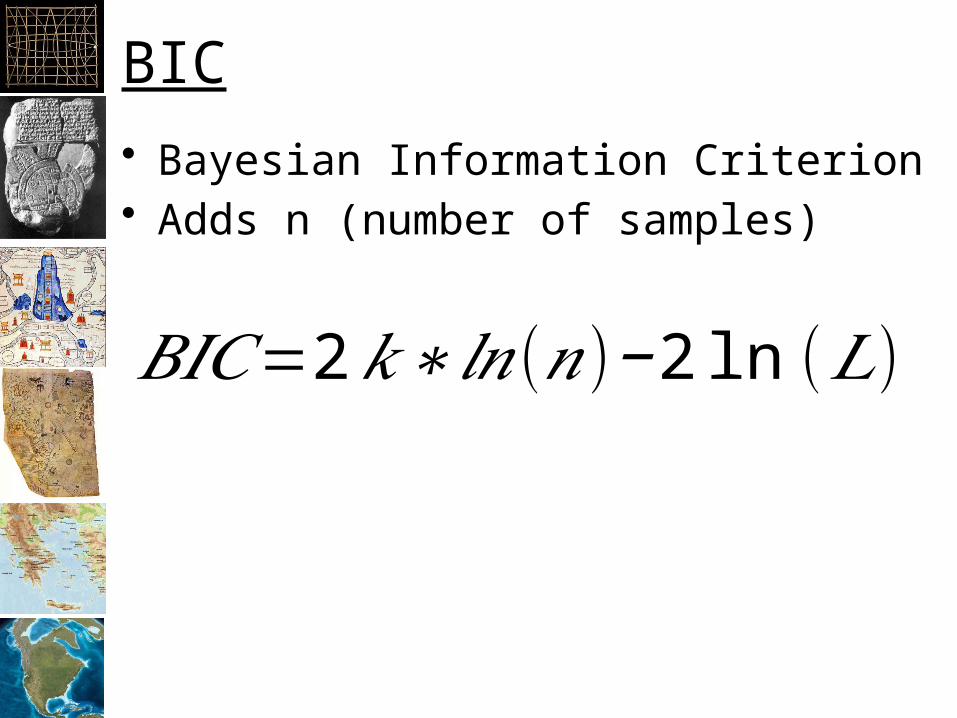
BIC
• Bayesian Information Criterion• Adds n (number of samples)
𝐵𝐼𝐶=2𝑘∗𝑙𝑛(𝑛)−2 ln (𝐿)
• The distance can also be expressed as:• is the expectation of so:
• Treating as an unknown constant:– = Relative Distance between g and f